Hyperbolic stochastic partial differential

equations with additive fractional Brownian sheet

Mohamed Erraoui∗

Faculte des Sciences SemlaliaDepartement de Mathematiques

Universite Cadi AyyadBP 2390, Marrakech, Maroc

David Nualart†

Facultat de MatematiquesUniversitat de Barcelona

Gran Via, 58508007, Barcelona, Spain

Youssef Ouknine‡,Faculte des Sciences Semlalia

Departement de MathematiquesUniversite Cadi Ayyad

BP 2390, Marrakech, Maroc

Abstract

Let BH,H′z , z ∈ [0, T ]2 be a fractional Brownian sheet with Hurst

parameters H, H ′ ≤ 12. We prove the existence and uniqueness of a strong

solution for a class of hyperbolic stochastic partial differential equationwith additive fractional Brownian sheet of the form Xz = x + BH,H′

z +R[0,z]

b(ζ, Xζ)dζ, where b(ζ, x) is a Borel function satisfying some growth

and monotonicity assumptions. We also prove the convergence of Euler’sapproximation scheme for this equation.

Keywords: Fractional Brownian sheet. Hyperbolic stochastic partialdifferential equations. Stochastic integrals. Euler’s scheme.

AMS Subject Classification: 60H05, 60H15.

1 Introduction

The motivation for the present work is to study the following hyperbolic stochas-tic partial differential equation

∂2u (s, t)∂s∂t

= b(s, t, u (s, t)) +∂2BH,H′

(s,t)

∂s∂t, s, t ∈ [0, T ]

u (s, 0) = u (0, t) = a,

(1)

∗Supported by Moroccan Program PARS MI 37†Supported by the DGES grant BFM2000-0598‡Supported by Moroccan Program PARS MI 37

1

where BH,H′= BH,H′

z , z ∈ [0, T ]2 is a fractional Brownian sheet with Hurst

parameter (H, H ′) ∈ (0,12)2. That is, BH,H′

is a centered Gaussian processwith covariance

RH,H′(z, z′) = E(BH,H′z BH,H′

z′ )= 1

4

s2H + (s′)2H − |s′ − s|2H

t2H′

+ (t′)2H′ − |t′ − t|2H′,

where z = (s, t) and z′ = (s′, t′). The nonlinear coefficient is a Borel functionb : [0, T ]2 × R→ R. The main results of the paper are:

(i) If b satisfies the linear growth condition:

|b(z, x)| ≤ C(1 + |x|), (2)

then Equation (1) has a unique weak solution.

(ii) If the function b is nondecreasing with respect to the second variable andbounded, then Equation (1) has a unique strong solution.

These results represent an extension to the two-parameter case of thoseproved in a recent work by Nualart and Ouknine [14] for the equation

Xt = x + BHt +

∫

[0,t]

b(s,Xs)ds,

where BHt is 1-parameter fractional Brownian motion. The result (ii) in the case

H = H ′ = 12 , i.e.when BH,H′

is an ordinary Brownian sheet, has been provedby Nualart and Tindel in [15].

We also show the convergence of the Euler’s approximation scheme for Equa-tion (1) under the assumptions given in (ii). A similar approximation result hasbeen established for several types of stochastic differential equations (see [4], [9],[10] and references therein).

A brief outline of the paper is as follows. In Section 2 we give some pre-liminaries on two-parameter fractional calculus. It is well-known that the mainapproach for constructing weak solutions to stochastic differential equations isthe transformation of drift via Girsanov theorem. Since the fractional Browniansheet has an integral representation of the form

BH,H′z =

∫

[0,z]

KH,H′(z, ζ)dWζ ,

where W is a standard Brownian sheet and KH,H′ is a square integrable kernel,the weak existence and uniqueness are easily established using a suitable ver-sion of Girsanov theorem. This is done in Section 3. In Section 4, a comparisontheorem based on the monotonicity of the coefficient is given. In Section 5, thestrong existence and uniqueness results are established. The proof is based onthe comparison theorem established in Section 5 and the equi-absolute continu-ity of the occupation measures of a certain class of approximations of u. Note

2

that this method has also been used to handle one-dimensional heat equationswith additive space-time white noise in [8]. Finally, in Section 6, using the re-sult of Section 5, we prove the convergence of Euler’s approximation scheme forEquation (1).

2 Preliminaries

2.1 Fractional calculus

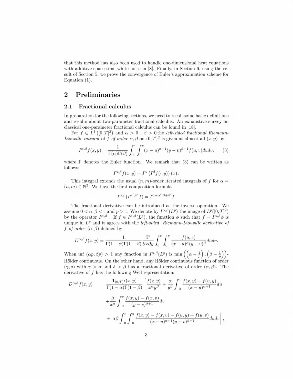
In preparation for the following sections, we need to recall some basic definitionsand results about two-parameter fractional calculus. An exhaustive survey onclassical one-parameter fractional calculus can be found in [18].

For f ∈ L1([0, T ]2

)and α > 0 , β > 0 the left-sided fractional Riemann-

Liouville integral of f of order α, β on (0, T )2 is given at almost all (x, y) by

Iα,βf(x, y) =1

Γ(α)Γ(β)

∫ x

0

∫ y

0

(x− u)α−1(y − v)β−1f(u, v)dudv, (3)

where Γ denotes the Euler function. We remark that (3) can be written asfollows:

Iα,βf(x, y) = Iα(Iβf(·, y)

)(x) .

This integral extends the usual (n,m)-order iterated integrals of f for α =(n, m) ∈ N2. We have the first composition formula

Iα,β(Iα′,β′f) = Iα+α′,β+β′f.

The fractional derivative can be introduced as the inverse operation. Weassume 0 < α, β < 1 and p > 1. We denote by Iα,β(Lp) the image of Lp([0, T ]2)by the operator Iα,β . If f ∈ Iα,β(Lp), the function φ such that f = Iα,βφ isunique in Lp and it agrees with the left-sided Riemann-Liouville derivative off of order (α, β) defined by

Dα,βf(x, y) =1

Γ(1− α)Γ(1− β)∂2

∂x∂y

∫ x

0

∫ y

0

f(u, v)(x− u)α(y − v)β

dudv.

When inf (αp, βp) > 1 any function in Iα,β(Lp) is min((

α− 1p

),(β − 1

p

))-

Holder continuous. On the other hand, any Holder continuous function of order(γ, δ) with γ > α and δ > β has a fractional derivative of order (α, β). Thederivative of f has the following Weil representation:

Dα,βf(x, y) =1(0,T )2(x, y)

Γ(1− α)Γ(1− β)

[f(x, y)xαyβ

+α

yβ

∫ x

0

f(x, y)− f(u, y)(x− u)α+1

du

+β

xα

∫ y

0

f(x, y)− f(x, v)(y − v)β+1

dv

+ αβ

∫ x

0

∫ y

0

f(x, y)− f(x, v)− f(u, y) + f(u, v)(x− u)α+1(y − v)β+1

dudv

],

3

where the convergence of the integrals at the singularity x = u or y = vholds in Lp-sense.

Recall that by construction for f ∈ Iα,β(Lp),

Iα,β(Dα,βf) = f

and for general f ∈ L1([0, T ]2) we have

Dα,β(Iα,βf) = f.

If f ∈ Iα+α′,β+β′ (L1), α ≥ 0, β ≥ 0, α′ ≥ 0, β′ ≥ 0 , sup(α + β, α′ + β′) ≤ 1 wehave the second composition formula

Dα,β(Dα′,β′f) = Dα+α′,β+β′f.

3 Existence of a weak solution, and pathwiseuniqueness property

In this section we introduce the notion of weak solution for a stochastic differen-tial equation with additive fractional Brownian sheet. We discuss the existenceand uniqueness of such solutions and the uniqueness in law for such equation.For the proof of the main results we follow the approach developed by Nualartand Ouknine in [14] for the one-parameter case, based on Girsanov theorem.

3.1 Girsanov transformation

Let (Ω,F , P ) be a probability space. If z1, z2 ∈ [0, T ]2, zi = (si, ti), i = 1, 2,we will write z1 ≥ z2 if s1 ≥ s2 and t1 ≥ t2. For any z1 ≥ z2, we set [z1, z2] =[s1, s2] × [t1, t2]. Let BH = BH,H′

z , z ∈ [0, T ]2 be a fractional Brownian

sheet with Hurst parameters 0 < H, H ′ ≤ 12

defined on the probability space

(Ω,F , P ). For each z ∈ [0, T ]2 we denote by FBz the σ-field generated by the

random variablesBH,H′

ζ , ζ ≤ z

and the sets of probability zero. We will say

that a stochastic process u =uz, z ∈ [0, T ]2

is FB

z -adapted if u(z) is FBz -

measurable for all z ∈ [0, T ]2. Given z1 = (s1, t1) ≤ z2 = (s2, t2) and a processX we denote by

4[z1,z2] (X) = X (s2, t2)−X (s2, t1)−X (s1, t2) + X (s1, t1)

the increment of X on the rectangle [z1, z2].We denote by E ⊂ H the set of step functions on [0, T ]2. LetH be the Hilbert

space defined as the closure of E with respect to the scalar product⟨1[0,z],1[0,z′]

⟩H = RH,H′(z, z′).

The mapping 1[0,z] −→ BH,H′z can be extended to an isometry between H

and the Gaussian space H1(BH,H′) associated with BH,H′

. We will denote thisisometry by ϕ −→ BH,H′

(ϕ).

4

The covariance kernel RH,H′(z, z′) can be written as

RH,H′(z, z′) =∫

[0,z∧z′]KH,H′(z, ζ)KH,H′(z′, ζ)dζ,

where [0, z ∧ z′] = [0, s ∧ s′]× [0, t ∧ t′] and KH,H′ is the square integrable kernelgiven by :

KH,H′(z, z′) = KH(s, s′)KH′(t, t′),

where KH , KH′are defined by (see [3]):

KH(s, s′) = Γ(H + 1

2

)−1 (s′ − s)H− 12 F (H − 1

2 , 12 −H,H + 1

2 , 1− s′

s)

KH′(t, t′) = Γ(H + 1

2

)−1 (t′ − t)H− 12 F (H − 1

2 , 12 −H, H + 1

2 , 1− t′

t),

F (a, b, c, z) being the Gauss hypergeometric function. Consider the linear oper-ator K∗

H,H′ from E to L2([0, T ]2) defined by

(K∗H,H′ϕ)(z) = KH,H′((T, T ) , z)ϕ(z)+

∫

[z,(T,T )]

(ϕ(ζ)− ϕ(z))∂2KH,H′

∂ζ(ζ, z)dζ.

For any pair of step functions ϕ and ψ in E we have⟨K∗

H,H′ϕ, K∗H,H′ψ

⟩L2([0,T ]2)

= 〈ϕ,ψ〉H .

This is an immediate consequence of the fact that(K∗

H,H′1[0,z]

)(ζ) = KH,H′(z, ζ).

As a consequence, the operator K∗H,H′ provides an isometry between the Hilbert

spaces H and L2([0, T ]2). Hence, the process W = Wz, z ∈ [0, T ]2 defined by

Wz = BH,H′((K∗

H,H′)−1 (1[0,z])) (4)

is a Brownian sheet, and the process BH,H′has an integral representation of

the formBH,H′

z =∫

[0,z]

KH,H′(z, ζ)dWζ . (5)

We refer to [1] for the proof of similar results in the one-parameter case.From (4) and (5) it follows that FB

z coincides with the filtration FWz gener-

ated by the Brownian sheet W . This filtration satisfies the following properties(see Cairoli and Walsh [2]):

(F1) FWz is increasing with respect to the partial order in [0, T ]2.

(F2) FWz is right-continuous, that is, for all z ∈ [0, T )2 we have ∩nFW

z+( 1n , 1

n )=

FWz .

5

(F3) FW0 contains the sets of probability zero.

(F4) For any 0 ≤ s, t ≤ T , the σ-fields ∨0≤u≤TFW(u,t) and ∨0≤v≤TFW

(s,v) areconditionally independent given FW

(s,t).

We will make use of the following definitions.

Definition 1 LetFz, z ∈ [0, T ]2

be a family of σ-fields satisfying properties

(F1)-(F4). A Brownian sheet W = Wz, z ∈ [0, T ]2 is called an Fz-Browniansheet if W is Fz-adapted and for any z1 ≤ z2 the increment 4[z1,z2] (W ) isindependent of the σ-field generated by W(u,v), u ≤ s1 or v ≤ t1.

Definition 2 LetFz, z ∈ [0, T ]2

be a family of σ-fields satisfying proper-

ties (F1)-(F4). A fractional Brownian sheet BH,H′= BH,H′

, z ∈ [0, T ]2is called an Fz-fractional Brownian sheet if the process W defined in (4) is anFz-Brownian sheet.

The operator KH,H′ , on L2([0, T ]2) associated with the kernel KH,H′ is anisomorphism from L2([0, T ]2) onto IH+1/2,H′+1/2(L2([0, T ]2)) and it can be ex-pressed in terms of fractional integrals as follows (see [3] for the one-parametercase):

(KH,H′h)(s, t) = I2H,2H′s

12−Ht

12−H′

I12−H, 1

2−H′sH− 1

2 tH′− 1

2 h, (6)

where h ∈ L2([0, T ]2).Given a process with integrable trajectories u = uz, z ∈ [0, T ]2 consider

the transformationBH,H′

z = BH,H′z +

∫

[0,z]

uζdζ. (7)

We can write

BH,H′z =

∫

[0,z]

KH,H′(z, ζ)dWζ +∫

[0,z]

uζdζ =∫

[0,z]

KH,H′(z, ζ)dWζ ,

where

Wz = Wz +∫

[0,z]

(K−1

H,H′

(∫

[0,·]uζdζ

)(η)

)dη. (8)

Notice that K−1H,H′

(∫[0,·] uζdζ

)belongs to L2([0, T ]2) almost surely if and only

if∫[0,·] uζdζ ∈ IH+1/2,H′+1/2(L2([0, T ]2)). As a consequence we deduce the

following version of the Girsanov theorem for the fractional Brownian sheet:

Theorem 3 LetFz, z ∈ [0, T ]2

be a family of σ-fields satisfying properties

(F1)-(F4). Suppose that BH,H′= BH,H′

, z ∈ [0, T ]2 is an Fz-fractionalBrownian sheet and W = Wz, z ∈ [0, T ]2 is the Fz-Brownian sheet givenby (4). Consider the shifted process (7) defined by an Fz-adapted process u =uz, z ∈ [0, T ]2 with integrable trajectories. Assume that:

6

i)∫[0,·] uζdζ ∈ IH+1/2,H′+1/2(L2([0, T ]2)), almost surely.

ii) E(ξT,T ) = 1, where

ξT,T = exp(− ∫

[0,T ]2

(K−1

H,H′

(∫[0,·] uζdζ

))(z) dWz

− 12

∫[0,T ]2

(K−1

H,H′

(∫[0,·] uζdζ

))2

(z) dz

)

Then the shifted process BH,H′is an Fz-fractional Brownian sheet with Hurst

parameter (H, H ′) under the new probability P defined by d ePdP = ξT,T .

Proof. The filtration Fz satisfies the properties (F1)-(F4) under thenew probability P (see [6]). By the extension of Girsanov theorem to two-parameter processes (see [6]) applied to the adapted and square integrableprocess K−1

H,H′

(∫[0,·] uζdζ

)we obtain that the process W defined in (8) is a

Fz-Brownian sheet under the probability P . Hence, the result follows.From (6) the inverse operator K−1

H,H′ is given by

K−1H,H′h (s, t) = s

12−Ht

12−H′

D12−H, 1

2−H′s H− 1

2 t H′− 12 D2H,2H′

h, (9)

for all h ∈ IH+ 12 ,H′+ 1

2 (L2([0, T ]2)). If h vanishes on the axes and is absolutelycontinuous, it can be proved that

K−1H,H′h (s, t) = sH− 1

2 tH′− 1

2 I12−H, 1

2−H′s

12−Ht

12−H′ ∂2h

∂s∂t. (10)

From (10) it follows that a sufficient condition for i) is∫ T

0

∫ T

0u2

ζdζ < ∞.

3.2 Existence of a weak solution

We are going to use the Girsanov transformation (Theorem 3) in order to es-tablish the existence of a weak solution for the following stochastic differentialequation:

Xz = x + BH,H′z +

∫

[0,z]

b(ζ, Xζ)dζ, z ∈ [0, T ]2, (11)

where b is a Borel function on [0, T ]2 × R.By a weak solution to equation (11) we mean a couple of Fz-adapted pro-

cesses(BH,H′

, X)

on a filtered probability space (Ω,F , P,Fz, z ∈ [0, T ]2

),

such that the filtration Fz satisfies the properties (F1)-(F4) and:

i) BH,H′is an Fz-fractional Brownian sheet in the sense of Definition 2.

ii) X and BH,H′satisfy (11).

7

Theorem 4 Suppose that b(z, x) satisfies the linear growth condition (2). ThenEquation (11) has a weak solution.

Proof. Set BH,H′z = BH,H′

z − ∫[0,z]

b(ζ, BH,H′

ζ + x)dζ. We claim that the

process uζ = −b(ζ, BH,H′

ζ + x) satisfies conditions i) and ii) of Theorem 3. Ifthis claim is true, under the probability measure P , BH,H′

z is a FBz -fractional

Brownian sheet, and(BH,H′

z , BH,H′z + x

)is a weak solution of (11) on the

filtered probability space (Ω,F , P ,FB

z , z ∈ [0, T ]2).

Set

vz = −K−1H,H′

(∫

[0,.]

b(ζ, BH,H′

ζ + x)dζ

)(z).

From (10) and the linear growth property of b we obtain

|vz| =∣∣∣sH− 1

2 tH′− 1

2 I12−H, 1

2−H′s

12−Ht

12−H′

b(z, BH,H′z + x)

∣∣∣= 1

Γ( 12−H)Γ( 1

2−H′)sH− 1

2 tH′− 1

2×∣∣∣∫[0,z]

(s− u)−12−H

u12−H (t− v)−

12−H′

v12−H′

b((u, v) , BH,H′

(u,v) + x)dudv∣∣∣

≤ cH,H′C(1 + |x|+

∥∥∥BH,H′∥∥∥∞

),

(12)where cH,H′ is a constant depending only on H , H ′ and T . From (10) it followsthat the operator (KH,H′)−1 preserves the adaptability property. Hence, theprocess vz is adapted and then condition ii) can be proved using a version ofNovikov criterion for two-parameter processes. Indeed, it suffices to show thatfor some λ > 0

supz∈[0,T ]2

E(exp

(λ |vz|2

))< ∞, (13)

which is an immediate consequence of (12) and the exponential integrability ofthe seminorm of a Gaussian process (see Fernique [5]).

3.3 Uniqueness in law

Let(BH,H′

, X)

be a weak solution of the stochastic differential equation (11)

defined in the filtered probability space (Ω,F , P,Fz, z ∈ [0, T ]2

). Define

uz = K−1H,H′

(∫

[0,.]

b(ζ, Xζ)dζ

)(z).

Let P defined by

dP

dP= exp

(−

∫

[0,T ]2uζdWζ − 1

2

∫

[0,T ]2u2

ζdζ

)(14)

8

We claim that the process uz satisfies conditions i) and ii) of Theorem 3. Infact, uz is an Fz-adapted process and taking into account that Xz has thesame regularity properties than the fractional Brownian sheet we deduce that∫[0,T ]2

u2ζdζ < ∞ almost surely. Finally, we can apply again Novikov theorem in

order to show that E(

d ePdP

)= 1, because by Gronwall’s lemma for integrals in

the plane‖X‖∞ ≤

(|x|+

∥∥∥BH,H′∥∥∥∞

+ CT 2)

eCT 2.

By Theorem 3 the process

Wz = Wz +∫

[0,z]

uζdζ

is an Fz-Brownian sheet under the probability P . In terms of the process Wz

we can writeXz = x +

∫

[0,z]

KH,H′(z, ζ)dWz.

Hence, then X−x is a fractional Brownian sheet with respect to the probabilityP with Hurst parameter equal to (H, H ′). As a consequence, we can easily proveas in [14] that the processes X −x and BH,H′

have the same distribution underthe probability P . In conclusion we have proved the following result:

Theorem 5 Suppose that b(z, x) satisfies the assumptions of Theorem 4. Thenall weak solutions have the same distribution.

4 Comparison theorem

The standard comparison theorem does not hold for hyperbolic partial differen-tial equations, as it is shown, for instance, in [13]. Nevertheless we can establisha comparison theorem for hyperbolic equations assuming the monotonicity ofone of the coefficients:

Theorem 6 Let u1 and u2 be two solutions of the deterministic equations

ui(z) = x + βz +∫

[0,z]

bi(ζ, ui(ζ))dζ, z ∈ [0, T ]2, (15)

i = 1, 2, where βz is a continuous function vanishing on the axes. Assume that

(j) For each z ∈ [0, T ]2 , b2(z, x) is a nondecreasing function of x(jj) |b2(z, x)− b2(z, y)| ≤ ρ (|x− y|) , for all z ∈ [0, T ]2

(jjj) b1(z, x) ≤ b2(z, x),

where ρ is concave, continuous, with ρ (0) = 0 and∫

0+

du

ρ (u)= +∞.

9

Then the solutions u1 and u2 satisfy

u1(z, x) ≤ u2(z, x).

Proof. Set

U(z) = u1(z)− u2(z) =∫

[0,z]

[b1(ζ, u1 (ζ))− b2(ζ, u2 (ζ))] dζ.

Using assertions (j)− (jjj), we get, for each z ∈ [0, T ]2

U(z) ≤ ∫[0,z]

[b2(ζ, u1 (ζ))− b2(ζ, u2 (ζ))] dζ

≤ ∫[0,z]

[b2(ζ, u1 (ζ))− b2(ζ, u2 (ζ))]1[0,+∞) (U(ζ)) dζ

≤ ∫[0,z]

ρ (U(ζ))1(−∞,0] (U(ζ)) dζ

=∫[0,z]

ρ (U+(ζ)) dζ.

This implies that

U+(z) ≤∫

[0,z]

ρ(U+(ζ)

)dζ,

and by Bihari’s Lemma for integrals in the plane, U+(z) = 0 on [0, T ]2 .We can also see that the above comparison theorem remains true under the

following assumption

(C)

(j) For each z ∈ [0, T ]2 , f(z, x) is nondecreasing function of x(jj) |f(z, x)− f(z, y)| ≤ ρ (|x− y|) , for all z ∈ [0, T ]2

(jjj) b1(z, x) ≤ f(z, x) ≤ b2(z, x)

where ρ is as before.

5 Existence of a strong solution

The purpose of this section is to discuss the existence of a strong solution ofEquation (11). For this we will make use of an approach similar to that con-

sidered by [16] in the case H = H ′ =12. In fact, there is no stochastic integral

in the Equation (11) and in the proof of the existence we just use the fact thatthe fractional Bownian sheet is a Gaussian process. Let us first recall somedefinitions and preliminaries results. For d ≥ 1, let us denote by B (

Rd)

theBorel σ-algebra on Rd and by λm the Lebesge measure on Rm.

Definition 7 Let M be the set of measures on B (Rd

). We say that M is equi-

absolutely continuous with respect to a given measure ν on B (Rd

)if for every

ε > 0 there exists a δ > 0 such that µ (A) < ε for all µ ∈M and all A ∈ B (Rd

)satisfying ν (A) < δ.

10

Definition 8 Let D be a domain in Rd and let X = Xz, z ∈ D be a mea-surable random field taking values in Rm. The measure defined on B (Rm) by

µX (A) = E(∫

D

1A (Xz) dz

), A ∈ B (Rm)

is called the occupation measure of X.

We next state a lemma whose proof is given by Gyongy in [7]. Let Xn =Xn (z) ; z ∈ D, n ≥ 1 be a sequence of Rm-valued random fields on a boundeddomain D ⊂ Rd and let fn, n ≥ 1 be a sequence of uniformly bounded func-tions fn : Rm → R such that the following conditions are satisfied:

(a) Xn (z) converges in probability to a random variable X (z) for everyz ∈ D.

(b) The occupation measures µXnof Xn form an equi-absolutely continuous

set of measures with respect to λm.(c) The functions fn converge to f in the measure λm on compact sets, i.e.

for every ε > 0 and R > 0,

limn→∞

λm x ∈ Rm : |x| < R, |fn (x)− f (x)| ≥ ε = 0.

We then have the following result:

Lemma 9 Suppose that Xn, X, fn and f verify (a)-(c). Then for every p ≥ 1

limn→∞

E(∫

D

|fn (Xn (z))− f (X (z))|p dz

)= 0

Let BH,H′= BH,H′

, z ∈ [0, T ]2 be a fractional Brownian sheet withHurst parameter (H, H ′) ∈ (

0, 12

)2. Fix M > 0 and denote by SM the set of allcontinuous process y on [0, T ]2 of the form

y(z) = x +∫

[0,z]

b(ζ)dζ + BH,H′z

where b(.) is an FBz -adapted process bounded by M and x ∈ R. Let also SM

be the set of continuous processes y on [0, T ]2 such that there exists a sequenceof processes (yn)n∈N of SM with

limn→∞

yn (z, ω) = y (z, ω)

for almost all (z, ω) ∈ [0, T ]2 × Ω. We will need the following lemma.

Lemma 10 Let un, n ≥ 1 be a family of processes of SM , u a process ofSM and

fn (z, x) , f (z, x) ; n ≥ 1, z ∈ [0, T ]2 , x ∈ R

a family of functions

verifying:

(i) un (z) converges to u (z) in probability for every z ∈ [0, T ]2

(ii) fn is bounded uniformly in n by a fixed constant M

(iii) fn converges to f in the Lebesgue measure on the compact sets of [0, T ]2 × R.

11

Then for every p ≥ 1,

limn→∞

E

(∫

[0,T ]2|fn (z, un (z))− f (z, u (z))|p dz

)= 0.

Proof. Conditions (a) and (c) of Lemma 9 are verified for Xn (z) = (z, un (z))and X (z) = (z, u (z)), and we have only to check condition (b). Suppose thatfor any z ∈ [0, T ]2

un(z) = x +∫

[0,z]

bn(ζ)dζ + BH,H′z

where bn(.) is an FBz -adapted process bounded by M . Set, for n ≥ 1,

ρn = exp(− ∫

[0,T ]2

(K−1

H,H′

(∫[0,·] bn(ζ)dζ

))ζdWζ

− 12

∫[0,T ]2

(K−1

H,H′

(∫[0,·] bn(ζ)dζ

))2

ζdζ

)

dPn = ρndP.

Since H, H ′ ≤ 12

and using that bn(.) are bounded by M , we get

∣∣∣K−1H,H′

(∫[0,·] bn(ζ)dζ

)∣∣∣ =∣∣∣sH− 1

2 tH′− 1

2 I12−H, 1

2−H′s

12−Ht

12−H′

bn(ζ)∣∣∣

≤ McH,H′ ,

where cH,H′ is the constant appearing in (12). It follows that for any α ≥ 1

E (ρ−αn ) = exp

(α

∫[0,T ]2

(K−1

H,H′

(∫[0,·] bn(ζ)dζ

))ζdWζ

+α2

∫[0,T ]2

(K−1

H,H′

(∫[0,·] bn(ζ)dζ

))2

ζdζ

)

≤ Cα

where Cα is a constant independent of n. From Girsanov theorem in the plane(see [6]), Pn is a probability measure, and under Pn, un(.) has the same law as(x + BH,H′

·)

under P . Let us denote by En the expectation with respect to Pn

and by Y the process(z, x + BH,H′

z

). If A ∈ B (

R3), by Schwartz inequality

we get

E(∫

[0,T ]21A (ζ, un(ζ)) dζ

)= En

(ρ−1

n

∫[0,T ]2

1A (ζ, un(ζ)) dζ)

≤[En

(ρ−2

n

)]1/2[En

(∫[0,T ]2

1A (ζ, un(ζ)) dζ)2

]1/2

≤ CT[En

(∫[0,T ]2

1A (ζ, un(ζ)) dζ)]1/2

≤ CT (µY (A))1/2

12

which ends the proof, since the law of(z, x + BH,H′

z

)is equivalent to λ3.

Now we are able to prove the existence and uniqueness result.

Theorem 11 Suppose that b : [0, T ]2×R→ R is a measurable function verifying

(H1) supz∈[0,T ]2

supr∈R

|b (z, r)| ≤ M < ∞

(H2) ∀ z ∈ [0, T ]2 , b (z, r) is a nondecreasing function of r.

Then there exists a unique FBz -adapted solution to Equation (11).

To prove the theorem we need the following lemma (see Lemma 2.4 in [15])which provides an increasing approximation of function satisfying assumptions(H1) and (H2) .

Lemma 12 Let b : [0, T ]2 × R → R is a measurable function verifying (H1)and (H2) . Then there exists a family of measurable functions

bn (z, x) ; n ≥ 1, z ∈ [0, T ]2 , x ∈ R

such that

· limn→∞

bn (z, x) = b (z, x) , dz ⊗ dx a.e.

· x 7→ bn (z, x) is nondecreasing, for all n ≥ 1, z ∈ [0, T ]2

· n 7→ bn (z, x) is nondecreasing, for all x ∈ R, z ∈ [0, T ]2

· bn (z, .) is Lipschitz uniformly in z, ∀n ≥ 1, with constant Ln

· supn≥1

supz∈[0,T ]2

supr∈R

|b (z, r)| ≤ M.

Proof. (Existence) We pick a family

bn (z, x) ; n ≥ 1, z ∈ [0, T ]2 , x ∈ R

as in Lemma 12. Then for any n ≥ 1, Equation (11) has a unique solutionwhich we denote by un. It follows from Theorem 6 that un is nondecreasingand bounded in n, and therefore it has a limit. We set

limn→∞

un (z) = u (z) .

By Lemma 10, we have

L1− limn→∞

∫

[0,z]

bn (ζ, un(ζ)) dζ =∫

[0,z]

b (ζ, u(ζ)) dζ,

which allows us to show that u satisfies Equation (11).(Uniqueness) Let v be another solution. Then for any n ≥ 1, v−un verifies,

v(z)− un(z) =∫[0,z]

[b(ζ, v (ζ))− bn(ζ, un (ζ))] dζ

≥ ∫[0,z]

[bn(ζ, u1 (ζ))− bn(ζ, u2 (ζ))] dζ

≥ −Ln

∫[0,z]

(v(ζ)− un(ζ))− dζ.

We deduce that v(z) ≥ un(z) a.s., and by a limit argument we show thatv(z) ≥ u(z) a.s. On the other hand the laws of v and u are the same, so weobtain v = u a.s.

13

6 Euler’s approximation scheme

In this section we study the convergence of Euler’s scheme for Equation (11).Throughout this section Cp denotes a constant which changes from line to line.To simplify the notation assume that T = 1. Inspired by [16], we define anapproximation scheme for the solution of equation (11) as follows. For anyn ≥ 1 and 0 ≤ i, j ≤ n we set

sni =

i

n, tnj =

j

n, zn

i,j =(sn

i , tnj)

We also set Ini,j =

[zni,j , z

ni+1,j+1

]if 0 ≤ i, j ≤ n− 1. For every n ≥ 1, we define

the random field un by

un (0, t) = un (s, 0) = x

4Ini,j

(un) = 1n2 bn

(zni,j , un

(zni,j

))+4In

i,j

(BH,H′

),

if 0 ≤ i, j ≤ n− 1

un (z) = un

(zni,j

)+ n

(un

(zni+1,j

)− un

(zni,j

))(s− sn

i )

+n(un

(zni,j+1

)− un

(zni,j

))(t− tni )

+n24Ini,j

(un) (s− sni ) (t− tni ) ,

if 0 ≤ i, j ≤ n− 1, z ∈ Ini,j .

(16)

We will refer to this scheme as Eq(bn, BH,H′

). Note that for z ∈ In

i,j , un (z)is obtained by Euler’s polygonal approximation. We assume the following as-sumptions:

(H3) supz∈[0,T ]2

supr∈R

|bn (z, r)| ≤ M.

(H4) limn→∞

supz∈[0,T ]2

|bn (z, r)− b (z, r)| = 0 dr − a.e.

We will show that the sequence un (., x) converge to u (., x) in Lp, p ≥ 2, uni-formly in z ∈ [0, 1]2 and x ∈ B where B is a compact subset of R. This is givenin the following theorem.

Theorem 13 Suppose that b(z, x) satisfies the assumptions of Theorem 11.Then the process un given by Eq

(bn, BH,H′

)verifies

limn→∞

supx∈B

E

(sup

z∈[0,1]2|un(z, x)− u(z, x)|p

)= 0.

14

We start with the following a priori estimates of un and u which we obtainusing assumptions H1 and H3.

Lemma 14 Assume that assumptions H1 and H3 hold. Then for every p > 2there exists a constant Cp > 0 such that

(i) supx∈B

supn≥1

E

(sup

z∈[0,1]2|un(t, x)|p

)≤ Cp.

(ii) supx∈B

E

(sup

z∈[0,1]2|u(t, x)|p

)≤ Cp.

For the following lemmas, we will need some additional notations. If z =(s, t) ∈ [0, 1]2 and n ≥ 1, we will set

kn (z) =(

[ns]n

,[nt]n

).

We also set, for a process X in [0, 1]2 and a measurable function f : [0, 1]×R→ R

f(X, kn) (z) = f(kn (z) , Xkn(z)).

Finally, we will denote by λ the Lebesgue measure in the plane. To be ableto apply the Skorohod embedding theorem and to prove the convergence ofthe Euler’s approximation scheme, we want to show the tightness of the fam-ily un(·, x), n ≥ 1 in C

([0, 1]2

). This is the reason for giving the following

lemma.

Lemma 15 Assume that assumptions H1 and H3 hold. Then for every p > 2there exists a constant Cp > 0 such that

(i) supx∈B

supn≥1

E(∣∣4[z1,z2]un(z, x)

∣∣p) ≤ Cp (λ ([z1, z2]))p(H∧H′) .

(ii) supx∈B

E(∣∣4[z1,z2]u(z, x)

∣∣p) ≤ Cp (λ ([z1, z2]))p(H∧H′) .

Proof. Suppose first that z1 = zni,j , z2 = zn

k,l with i < k and j < l. We have

un(zni,j , x) = x + BH,H′

zni,j

+∫

[0,zni,j]

bn (un, kn) (ζ)dζ,

and4[zn

i,j , znk,l]un = 4[zn

i,j , znk,l]B

H,H′+

∫

[zni,j , zn

k,l]bn (un, kn) (ζ)dζ.

It follows that

E( ∣∣4[z1,z2](un)

∣∣p) ≤ Cp (λ ([z1, z2]))p(H∧H′) .

The cases where z1 and z2 are not of this form are treated as in [15].The next two lemmas provided the main ingredients to show that the limit

of un (·) satisfies the Equation (11).

15

Lemma 16 Let

un (z) ; n ≥ 1, z ∈ [0, 1]2

be the sequence of processes con-structed by (16). Then, for any p > 1 and 0 < ε < 1, there exists Nε and Kp,ε

such that for any measurable bounded function h : [0, 1]2 × R→ R and n > Nε

E

[∫

[ε,1]2|h (z, un (kn (z)))|p dz

]≤ Kp,ε ‖h‖p .

Moreover, if there exists a subsequence

unk(z) ; k ≥ 1, z ∈ [0, 1]2

converging

dP ⊗ dz a.s. to a process u, the inequality still holds for u.

Proof. For any z ∈ [0, 1]2, we have

un(kn (z)) = x +∫

[0,kn(z)]

bn(un, kn) (ζ) dζ + BH,H′

kn(z)

Set, for n ≥ 1,

ρn = exp(− ∫

[0,1]2

(K−1

H,H′

(∫[0,·] bn(un, kn)(ζ)dζ

))ζdWζ

− 12

∫[0,1]2

(K−1

H,H′

(∫[0,·] bn(un, kn)(ζ)dζ

))2

ζdζ

)

dPn = ρndP

Since H, H ′ ≤ 12

and using that bn(.) is bounded by M , we get, as in the proof

of Lemma 10, the estimate E (ρ−αn ) ≤ Cα, where Cα is a constant independent

of n. From Girsanov theorem in the plane (see [6]), Pn is a probability measure,and under Pn, un(kn (z)) has the same law as the process

(x + BH,H′

kn(z)

)under

P . In particular un (kn (z)) has the law N

(x,

([ns]n

)2H ([nt]n

)2H′). We denote

by p (r, z) the probability density of un (kn (z)) under Pn. Let us denote byEn the expectation with respect to Pn and by Y the process

(x + BH,H′

z

). By

Holder’s inequality

E[∫

[ε,1]2|h (ζ, un (kn(ζ)))|p dζ

]= En

[ρ−1

n

∫[ε,1]2

|h (ζ, un (kn(ζ)))|p dζ]

≤ C[En (ρ−q

n )]1/q [

En

∫[ε,1]2

|h (ζ, un (kn(ζ)))|p dζ]1/p

≤ C[En

∫[ε,1]2

|h (ζ, un (kn(ζ)))|p dζ]1/p

≤ C(∫

[ε,1]2

∫R |h (ζ, r)|p p (kn(ζ), r) drdζ

)1/p

≤ C

(sup

z∈[ε,1]2supr∈R

p (z, r)

)‖h‖p

if n ≥(

2ε

)1/(H∧H′).

16

Lemma 17 Let

un (z) ; n ≥ 1, z ∈ [0, 1]2

be the sequence of processes con-structed by (16) and um (z) ; m ∈ J a subsequence converging dP ⊗ dz a.s.to a process u . Then, for any 0 < ε < 1, p > 1

limm→∞, m∈J

E

[∫

[ε,1]2|bm (um, km ) (z)− b (z, u (z) )|p dz

]= 0.

The proof of this lemma is analogous to that of Lemma 3.6 in [15].Now we are ready to prove the convergence of Euler’s approximation scheme.Proof of Theorem 13. Assume that there exist δ > 0, x ∈ R and

a sequence of natural numbers (n(j))j≥0 and a sequence of real numbers and(xn(j)

)j≥0

converging to x such that

δ ≤infjE

(sup

t∈[0,1]

∣∣un(j)(z, xn(j))− u(z, x)∣∣p

).

We claim that this assumptions leads to a contradiction with the hypotheses ofthe Theorem. To simplify the notation set un = un(j) and xn = xn(j). From

Lemma 15 it follows that the law of the process(un(., xn), u(., xn), BH,H′

)

is tight on C([0, 1]2

)⊗3

, where u(., xn) is the solution of (11) and un(., xn) isconstructed by (16) with the initial data xn. By the Skorohod theorem there ex-

ists a probability space(Ω, F , P

)and a sequence

(un(., xn), vn(., xn), BH,H′

n

)

with the same distribution as(un(., xn), u(., xn), BH,H′

)which converges al-

most surely to(u (., x) , v (., x) , BH,H′

)in C

([0, 1]2

)⊗3

. Moreover, for every

z ∈ [ε, 1]2 with the notation kn (z) = zni,j , we can see that

un(z, xn) = xn +∫[ε,z]

bn (kn, un ) (ζ) dζ + BH,H′n (kn (z))

− ∫[kn(z),z]

bn (kn, un ) (ζ) dζ +∫

Cεbn (kn, un ) (ζ) dζ

+A1

whereA1 (z) = n

(un

(zni+1,j

)− un

(zni,j

))(s− sn

i )

+n(un

(zni,j+1

)− un

(zni,j

))(t− tni )

+n24Ini,j

(un) (s− sni ) (t− tni ) ,

and Cε = [0, 1]2\(ε, 1]2. On the other hand,

vn(z, xn) = xn +∫

[0,z]

b (ζ, vn(ζ, xn) ) dζ + BH,H′z .

17

Applying Lemma 15 and assumption (H3), we deduce the following estimates

E (|A1 (z)|) ≤ 3Cp

nH∧H′

E(∣∣∣

∫[kn(z),z]

bn (kn, un ) (ζ) dζ∣∣∣)≤ M

n2

E(∣∣∣

∫Cε

bn (kn, un ) (ζ) dζ∣∣∣)≤ 2Mε.

Letting n tend to infinity we can easily see that u (., x) and v (., x) are two solu-tions of Equation (11) on the probability space

(Ω, F , P

)with the fractional

Brownian sheet BH,H′ and the same initial data. On the other hand, using thestatement (i) of Lemma 14 we have

0 < δ ≤ E(

supz∈[0,1]2

|u(t, x)− v(t, x)|p)

= lim infnE

(sup

z∈[0,1]2|un(t, xn)− vn(t, xn)|p

).

We may notice finally that, by the pathwise uniqueness, we have u (., x) = v (., x)almost surely. That is a contradiction.

Acknowledgement 18 This work was completed during a stay of YoussefOuknine at the IMUB (Institut de Matematica de la Universitat de Barcelona).He would like to thank the IMUB for hospitality and support.

References

[1] E. Alos, O. Mazet and D. Nualart: Stochastic calculus with respect toGaussian processes. Annals of Probability 29 (2001), 766-801.

[2] R. Cairoli and J. Walsh: Stochastic integrals in the plane. Acta Mathemat-ica 134 (1975), 111-183.

[3] L. Decreusefond and A. S. Ustunel: Stochastic Analysis of the fractionalBrownian Motion. Potential Analysis 10 (1999), 177-214.

[4] M. Erraoui and Y. Ouknine: Approximations des equations differentiellesstochastiques par des equations a retard. Stochastics and Stochastics Re-ports 46 (1994), 53-62.

[5] X. M. Fernique: Regularite des trajectoires de fonctions aleatoires gaussi-ennes. In Ecole d’ete de Saint-Flour IV (1974), Lecture Notes in Mathe-matics 480, 2-95.

[6] X. Guyon and B. Prum: Semi-martingales a indice dans R2. These, Uni-versite de Paris Sud, 1980.

18

[7] I. Gyongy: On non-degenerate quasi-linear stochastic partial differentialequations. Potential Analysis 4 (1995), 157-171.

[8] I. Gyongy and E. Pardoux: On quasi-linear stochastic partial differentialequations. Probab. Theory Rel. Fields 94 (1993), 413-425.

[9] I. Gyongy and N. Krylov: Existence of strong solutions for Ito’s stochasticequations via approximations, Probab. Theory Rel. Fields 105 (1996),143-158.

[10] I. Gyongy and D. Nualart: Implicit scheme for stochastic parabolic partialdifferential equations driven by space-time white noise. Potential Analysis7 (1997), 725-757.

[11] S. Moret and D. Nualart: Onsager-Machlup functional for the fractionalBrownian motion. Probab. Theory Rel. Fields. To appear.

[12] S. Nakao: On the pathwise uniqueness of solutions of one-dimensionalstochastic differential equations. Osaka J. Math. 9 (1972), 513-518.

[13] D. Nualart: Some remarks on a linear stochastic differential equation. Stat.and Probab. Letters 5 (1987), 231-234.

[14] D. Nualart and Y. Ouknine: Regularization of differential equations byfractional noise. Stoch. Proc. Appl. To appear.

[15] D. Nualart and S. Tindel: On two-parameter non-degenerate Brownianmartingales. Bull. Sci. Math. 122 (1998), 317-335.

[16] D. Nualart and S. Tindel: Quasilinear stochastic hyperbolic differentialequations with nondecreasing coefficient. Potential Analysis 7 (1997), 661-680.

[17] I. Norros, E. Valkeila and J. Virtamo: An elementary approach to a Gir-sanov formula and other analytical results on fractional Brownian motion.Bernoulli 5 (1999), 571-587.

[18] S. G. Samko, A. A. Kilbas and O. I. Mariachev: Fractional integrals andderivatives (Gordon and Breach Science 1993).

[19] A. Ju. Veretennikov: On strong solutions and explicit formulas for solutionsof stochastic integral equations. Math. USSR Sb. 39 (1981), 387-403.

[20] A. K. Zvonkin: A transformation of the phase space of a diffusion processthat removes the drift. Math. USSR Sb. 22 (1974), 129-149.

19