risk indifference pricing and backward stochastic differential equations
TRANSCRIPT

Risk indifference pricing and backward stochastic differential equations X. De Scheemaekere We study a risk indifference pricing problem in incomplete markets: The (seller’s) risk indifference price is the initial payment that makes the risk involved for the seller of a contract equal to the risk involved if the contract is not sold, with no initial payment. We provide an explicit formula for the risk indifference price as the solution of a backward stochastic differential equation solving a zero-sum stochastic differential game problem. JEL Classifications: C61; G12; G13 Keywords: Indifference pricing; Risk measure; Backward stochastic differential equation; Stochastic differential zero-sum game.
CEB Working Paper N° 08/027 September 2008
Université Libre de Bruxelles – Solvay Business School – Centre Emile Bernheim ULB CP 145/01 50, avenue F.D. Roosevelt 1050 Brussels – BELGIUM e-mail: [email protected] Tel. : +32 (0)2/650.48.64 Fax : +32 (0)2/650.41.88
Risk indifference pricing and backwardstochastic differential equations
Xavier De Scheemaekere∗
October 6, 2008
Abstract
We study a risk indifference pricing problem in incomplete markets: The(seller’s) risk indifference price is the initial payment that makes the risk involvedfor the seller of a contract equal to the risk involved if the contract is not sold,with no initial payment. We provide an explicit formula for the risk indifferenceprice in terms of solutions of a backward stochastic differential equations solvingzero-sum stochastic differential game problems.
Keywords: Indifference pricing; Risk measure; Backward stochastic differ-ential equation; Stochastic differential zero-sum game.JEL Classification: C61; G12; G13
1 IntroductionIn a complete market, it is well known that there is a unique linear arbitrage-free pricing rule at time t = 0 for a contract with payoff G at time t = T . Thisprice is the expectation of the discounted payoff G with respect to the so-calledequivalent martingale measure. If one would like to take a more realistic view ofthe financial world, one has to think again about some fundamental questionsconcerning pricing and hedging in an incomplete market.In incomplete markets, however, the situation is not so clear. There are
infinitely many equivalent martingale measures and it is not clear which one touse in the pricing formula. In fact, the no-arbitrage assumption provides a set ofequivalent martingale measures and an interval of arbitrage-free prices. Thereis no exact replication to provide a unique price. One possibility for a trader isto charge a super-replication (super-hedging) price for selling an option so thathe can trade to eliminate all risks. However, this price is usually forbiddingly
∗F.R.S.-F.N.R.S. Research Fellow; Université Libre de Bruxelles, Solvay Brussels Schoolof Economics and Management, Centre Emile Bernheim, CP 145/1, Av. F.D. Roosevelt, 50,1050 Brussels, Belgium ; Phone: +32.2.650.39.59; E-mail: [email protected]
1
high. For example, the super-replication price for a European option is thetrivial upper bound of the no-arbitrage interval. In the most common exampleof a call option, the super-hedging strategy is to buy and hold and thereforethe price of the call is equal to the initial stock price, which is excessivelyexpensive. In other words, the gap between upper (seller) and lower (buyer)hedging price is too wide. Since super-hedging is not a realistic solution undersuch circumstance, the trader is restricted to charging a reasonable price, findinga partial hedging strategy according to some optimality criterion, and bearingsome risks in the end.There are two major approaches that have been developed in searching for
solutions of pricing and hedging in incomplete markets. One is to pick a specificmartingale measure for pricing according to some optimality criterion, and theother is utility based derivative pricing. In brief, the pitfall of the first method isthat it does not provide financially reasonable hedging strategies, if at all, whilstthe second one requires the trader to explicitly write down his utility function,which is quite unusual in practice (see [29] for references and comments on otherapproaches that try to extend arbitrage pricing theory to incomplete markets).In this work, we investigate a pricing formula in incomplete markets based
on the risk indifference principle. As in [29] and [25], we replace the criterion ofmaximising utility by minimizing risk exposure because the latter is more oftenused in practice and because it keeps the central importance of optimal hedgingto the theory of pricing. Another reason to adopt risk measure pricing is thatit is quite a natural extension to the idea of pricing and hedging in completemarkets. In the Black-Scholes world, there is a unique risk-neutral measure, thetrader quotes a unique price, does delta-hedging, and presumably, ends up withno risk and no profit: it is the core of the absence of arbitrage underlying theBlack-Scholes machinery. An extension of this idea into an incomplete marketwould be that the trader buys or sells the option for an amount such that withactive hedging his risk exposure will not increase at expiration. Importantly,we will see that risk indifference pricing reduces the gap between seller’s andbuyer’s prices.In Section 2, we introduce the principle of risk indifference pricing, compare
it to classical utility indifference pricing and state an important representationtheorem (in fact, a dual characterization). Then, we show that the risk indif-ference price is the solution of two (zero-sum) stochastic differential games.In Section 3, we recall some results in the theory of backward stochastic
differential equations (BSDE, for short), mainly an important uniqueness andexistence result for BSDEs with Lipschitz coefficient and a comparison theorem.Then, we recall how BSDE theory applies to zero-sum stochastic differentialgame problems. In fact, results on BSDEs lead to very simple approach for theexistence of optimal strategies in such games.In Section 4, we use these results to solve our "stochastic differential pricing
games" and find an explicit description for the risk indifference price (Section5).We then relate our results to [14] who uses properties of parabolic partial
differential equations in order to solve stochastic differential games (Section 6).
2
We follow the spirit of [25] who study a similar risk indifference pricingproblem although [25] use stochastic control theory and PDE methods in thejump diffusion case, whereas we limit ourselves to the diffusion case.Our main contribution is to provide an explicit formula for the solution of
a general risk indifference pricing problem. The novelty is in combining BSDEapproach to zero-sum stochastic differential games and a dual formulation of arisk indifference pricing problem.As regard literature in general, we use results in the theory of BSDEs ([9],
[10]), in particular in the theory of BSDEs applied to stochastic differential gameproblems ([11], [17], [16]) to examine pricing problems in incomplete marketsvia BSDE techniques ([2], [20]) in a risk indifference framework ([23], [25], [29]).
2 Pricing in incomplete marketsLet us examine formally how risk indifference pricing naturally extends utilityindifference pricing.Utility indifference pricing. This pricing principle was introduced by
[19]. It is based on a given (chosen) utility function U : R→ R ∪ −∞.(i) If a person sells a liability to pay out the amount G(ω) at time T and
receives an initial payment p for such a contract, the maximal expected utilityfor the seller is
VG(x+ p) = supπ∈Π
E[U(X(π)x+p(T )−G)],
where x is the seller’s wealth before the contract is being made and X(π)x+p(T )
the final value of the self-financing replicating portfolio (wealth process) withrespect to G, with initial value x + p, where the supremum is taken over alladmissible portfolios.(ii) If, on the other hand, no such contract is made, the maximal expected
utility is
V0(x) = supπ∈Π
E[U(X(π)x (T ))].
The (seller’s) utility indifference price is the value of the initial payment pthat makes the seller indifferent to whether sell the contract or not, i.e., p is thesolution p = putility of the equation
VG(x+ p) = V0(x).
To find p one has to solve the two stochastic control problems above. Ingeneral, this is difficult and an explicit solution is known only in special casesand only for exponential utility functions such as
U(x) = −1ce−cx; x ∈ R,
3
where c > 0 is a constant. See e.g. [24].Before turning to risk indifference pricing, let us have a closer look at the
concept of risk measure. The problem is that of quantifying the risk of a financialposition. Such a position can be described by the corresponding payoff profile,that is, by a real-valued function X on some set of possible scenarios. In aprobabilistic model, specified by a probability measure on scenarios, one couldfocus on the resulting distribution of X and try to measure risk in terms ofquantiles or moments. Note that a classical measure of risk such as the variancedoes not capture a basic asymmetry in the financial interpretation of X becauseit is the downside risk that matters. This asymmetry is taken into account bymeasures of risk such as Value at Risk (VaR) which are based on quantiles forthe lower tail of the distribution. Value at Risk, however, fails to satisfy somenatural consistency requirements. In fact, optimizing a portfolio with respectto VaR may lead to a concentration of the portfolio in one single asset withsufficiently small default probability, but with an exposure to large losses. Suchobservations have motivated the systematic investigation of measures of riskthat satisfy some basic axioms, as initiated by [3] for coherent risk measuresand by [13] for convex risk measures.We assume that uncertainty is described through a measurable space (Ω, F )
— at this stage, we do not need to assume that a probability measure is given onΩ. In this context, Ω can be thought of as a fixed set of scenarios. A financialposition is described by a mapping X : Ω → R where X(ω) is the discountednet worth of the position at the end of the trading period if the scenario ω ∈ Ωis realized. Our aim is to quantify the risk of X by some number ρ(X), whereX belongs to a certain class F of financial positions.
Definition 1 The functional ρ : F → R is a convex risk measure if, for any Xand Y in F, it satisfies the following properties:
• Monotonicity: If X≤ Y, then ρ(X) ≥ ρ(Y ).
• Translation invariance: If m∈ R, then ρ(X +m) = ρ(X)−m.
• Convexity: ρ(λX + (1− λ)Y ) ≤ λρ(X) + (1− λ)ρ(Y ), for 0 ≤ λ ≤ 1.
A convex risk measure is coherent if it satisfies also:
• Positive homogeneity: If λ ≥ 0, then ρ(λX) = λρ(X).
In many situations, however, risk may grow in a non-linear way as the size ofthe position increases, for example if liquidity cannot be assured in the market.For this reason, we do not insist on positive homogeneity. Instead, our focuswill be on convex measures of risk.
Risk indifference pricing. The purpose of this work is to study a pricingprinciple based on risk rather than utility. Thus the starting point is a givenconvex risk measure
4
ρ : F → R
where F is a set of functions (random variables on a probability space) tobe specified. We may regard F as the family of all possible financial positionsat time T, and if f ∈ F , then ρ(f) is the amount that has to be added to f tomake the financial position acceptable (in some sense). We now argue as in theutility indifference case:
(i) If a person sells a contract which guarantees a payoff G(ω) ∈ F at timeT and receives an initial payment p for this, then the minimal risk involved forthe seller is
ΦG(x+ p) = infπ∈Π
ρ(X(π)x+p(T )−G).
(ii) If, on the other hand, no contract is sold, and hence no initial paymentis received, then the minimal risk for the person is
Φ0(x) = infπ∈Π
ρ(X(π)x (T )).
Definition 2 The (seller’s) risk indifference price p = prisk of the claim G ∈ Fis the solution of the equation
ΦG(x+ p) = Φ0(x). (1)
Definition 3 Thus prisk is the initial payment that makes a person risk in-different between selling the contract with liability payoff G and not selling thecontract (and not receiving any payment either).
We will use the following representation of convex risk measures:
Theorem 4 ([13],[15]) A map ρ : F → R is a convex risk measure if and onlyif there exists a family L of measures Q¿P on FT and a closed convex “penaltyfunction” ζ : L→ R ∪ +∞ with inf
Q∈Lζ(Q) = 0 such that
ρ(x) = supQ∈L
EQ[−X]− ζ(Q) ; X ∈ F. (2)
In view of this (dual) representation we see that choosing a risk measure ρ isequivalent to choosing the family L of measures and the penalty function ζ. Theabove characterization encompasses risk measures that are of practical impor-tance, such as the much used CVaR ([7], [28]), the spectral (quantile weighted)risk measure Generalized CVaR ([1]) or even entropy-based risk measures ([4],[8]). Note that if we choose ζ= 0 then ρ becomes a coherent risk measure ([3]).In this perspective, the risk indifference pricing model we develop hereun-
der preserves the advantage of utility indifference pricing, mainly, its economic
5
justification ([18]) while avoiding the limitations of utility indifference pricing —essentially the lack of explicit calculations outside exponential utility models —by including pricing measures that are highly amendable to practical applica-tions.Using (2) we see that the problem of finding the risk indifference price p =
prisk given in (1) amounts to solving the following two zero-sum stochasticdifferential game problems:Find ΦG(x+ p) and an optimal pair (π∗, Q∗) ∈ Π× L such that
ΦG(x+ p) = infπ∈Π
µsupQ∈L
nEQ[−X(π)
x+p(T ) +G]− ζ(Q)o
and (3)
Φ0(x) = infπ∈Π
µsupQ∈L
nEQ[−X(π)
x (T )]− ζ(Q)o
,
for a given family of measures L and a given (convex) penalty function ζ.Note that with this representation the risk indifference pricing equation (1)reduces, under Black-Scholes assumptions, to the well-known risk-neutral equa-tion; hence the risk indifference pricing method generalizes the Black-Scholesmethod in a consistent way.The optimal pair (π∗,Q∗) we are looking for is a saddle point for the games
in (3) in the sense that whilst the seller tries to minimize the risk of the trans-action over his possible financial strategies, the “market” tries to maximize thecorrected expected loss over a set of generalized scenarios, where correctiondepends on scenarios. Of course, this interpretation is only valid when the mea-sures Q are probability measures. We call such problems stochastic differentialpricing games.In the sequel, we will make a choice of L which makes it possible to solve
such games explicitly using BSDEs. Before, we summarize the results we needon BSDE theory and on solutions to zero-sum stochastic differential games.
3 Preliminary results
3.1 Backward stochastic differential equations
From now on, we suppose given a probability space (Ω, F, P ) on which is defineda multi-dimensional Brownian motion W := (Wt)t≤T . Unless specified, we takeW to be d-dimensional. Let us denote by
©FWt := σ(Ws, s ≤ t)
ªt≤T the natural
filtration of W and its completion with the P-null sets of F . Ftt≤T satisfiesthe usual conditions, i.e., it is right-continuous and complete. Denoting by Ethe expectation with respect to P, we define the following spaces:
• Mn the set of Ft-progressively measurable, Rn-valued processes on Ω ×[0, T ]
6
• L2n(Ft) =nη : Ft −measurable Rn-valued random variable s.t. E
h|η|2
i<∞
o• S2n(0, T ) =
½ϕ ∈Mn with continuous paths s.t. E
∙supt≤T
|ϕt|2
¸<∞
¾
• H2n(0, T ) =
⎧⎨⎩Z ∈Mn s.t. E
⎡⎣ TZ0
|Zs|2 ds
⎤⎦ <∞
⎫⎬⎭• H1
n(0, T ) =
⎧⎪⎨⎪⎩Z ∈Mn s.t. E
⎡⎢⎣⎛⎝ TZ0
|Zs|2 ds
⎞⎠12
⎤⎥⎦ <∞
⎫⎪⎬⎪⎭ .
Let us now introduce the notion of multi-dimensional BSDE.
Definition 5 Let ξT ∈ L2m(FT ) be a Rm-valued terminal condition and let g bea Rm-valued coefficient, Mn⊗B(Rm×Rm×d)-measurable. A solution for the m-dimensional BSDE associated with parameters (g, ξT ) is a pair of progressivelymeasurable processes (Y,Z) := (Yt, Zt)t≤T with values in Rm ⊗Rm×d such that
Yt = ξT +
TZt
g(s, Ys, Zs)ds−TZt
ZsdWs, 0 ≤ t ≤ T (4)
Y ∈ S2m, Z ∈ H2m×d
The differential form of the equation is
−dYt = g(t, Yt, Zt)dt− ZtdWt, YT = ξT
Hereafter g is called the coefficient and the terminal value of the BSDE.
Under some specific assumptions on the coefficient g, the BSDE (4) has aunique solution. The standard assumptions (H1) are the following:
• g(t, 0, 0)t≤T ∈ H2m.
• ∃C ≥ 0 s.t. ∀(y, y0, z, z0) |g(ω, t, y, z)− g(ω, t, y0, z0)| ≤ C(|y − y0|−|z − z0|),dt⊗ dP − a.e.
That is, there exist a constant C such that g is uniformly Lipschitz withrespect to (y, z ).
Theorem 6 ([10],[26]) Under the standard assumptions (H1), there exists aunique solution (Y, Z) of the BSDE with parameters (g, ξT ).
7
In the one-dimensional case, i.e., when m = 1, we have a comparison theo-rem, which is an important tool in the study of one-dimensional BSDEs. It isthe equivalent of the maximum principle when working with PDEs. We state itunder (H1) but similar versions hold for weaker hypotheses ([10]).
Theorem 7 ([9]) Let us consider the solutions (Y, Z) and (Y’, Z’) of twoBSDEs with parameters (g0, ξT ) and (g, ξ
0T ). Only g is assumed to satisfy (H1).
If ξ0T ≤ ξT P- a.s. and ∀(y, z), g0(ω, t, Y 0t , Z
0t) ≤ g(ω, t, Y 0
t , Z0t), dt ⊗ dP − a.e.,
then
∀(y, z), Y 0t ≤ Yt, ∀t ∈ [0, T ] P − a.s.
The following result gives an explicit representation of the solution to a one-dimensional linear BSDE. It proves very useful for applications in stochasticdifferential games.
Proposition 8 ([9]) Let (β, μ ) be a bounded (R,Rd)- valued progressively mea-surable process, ϕ be an element of H2
1 (0, T ) and ξT ∈ L21(0, T ). We considerthe following linear BSDE:
−dYt = (ϕt + βtYt + μtZt)dt− ZtdWt, YT = ξT (5)
Equation (5) has a unique solution (Y,Z) ∈ S21(0, T ) × H2d(0, T ) and Y is ex-
plicitly given by
Yt = E
⎡⎣ξTΓt,T + TZt
Γt,sϕsds|Ft
⎤⎦ (6)
where (Γt,s)s≥t is the adjoint process defined by the forward linear SDE
dΓt,s = Γt,s(βsds+ μsdWs), Γt,t = 1 (7)
satisfying the flow property Γt,sΓs,u = Γt,u, ∀t ≤ s ≤ u, P- a.s.
3.2 Zero-sum stochastic differential games
We suppose the evolution of a system described by a Rd-valued SDE:
dxt = f(t, x., ut, vt)dt+ σ(t, x.)dWt, 0 ≤ t ≤ T ; x0 = x ∈ Rd.A zero-sum stochastic differential game goes as follows. A player J1 (resp.
J2) chooses a feedback control u (resp. v), with the object of maximizing (resp.minimizing) the payoff
J(u, v) := E
⎡⎣ TZ0
h(s, x., us, vs)ds+Ψ(xT )
⎤⎦ .
8
We insist that we write x.(ω) instead of xt(ω), because h may depend on theentire path x.(ω) up to time t, and not just on the value xt(ω). This means thatwe do not need any kind of Markovian assumptions on the considered functions.Indeed, the Markovian case is the particular situation when we take xt(ω) forx.(ω).The above results on the solutions of BSDEs allow one to solve the game in
a very simple way.Let C be the space of continuous functions from [0, T ] into Rd endowed with
the uniform norm and let D be a σ-algebra on [0, T ]× C such that if F t is theσ-algebra of C generated by the coordinate functions xs|x ∈ C → xs, s ≤ t,D denotes the F t-progressively measurable σ-algebra (see [12] for more details).Let σ be a function from [0, T ]× C into Rd×d such that
• σ is D-mesurable.
• ∀t ∈ [0, T ], ∀w ∈ C, σ(t, w) is invertible and there exists a constant ksuch that
¯σ−1(t, w
¯≤ k(1 + kwkδt ) for some constant δ, where kwkt =
sups≤t
|w(s)| , t ≤ T .
• ∀t ∈ [0, T ], ∀w,w0 ∈ C, there exists a constant k such that |σ(t, w)− σ(t, w0)| ≤k kw − w0kt .
• ∀t ∈ [0, T ], ∀w ∈ C, there exists a constant k such that |σ(t, w)| ≤ k(1 +kw0kt).
The first condition is a usual measurability condition. The last two condi-tions are necessary for classical existence and uniqueness results on SDE. Thesecond condition on the inverse of σ is natural in stochastic differential games.Note that it is weaker than the usual boundedness. However, [11] proved thatPu,v (defined hereunder) is still a probability under that assumption, which issufficient for our purpose.Then, the equation
dxt = σ(t, x.)dWt, 0 ≤ t ≤ T ; x0 = x ∈ Rd, (8)
has a unique solution xt ([21], [27]), which describes the dynamics of thesystem without control.The player J1 (resp. J2) acts with a M.-measurable stochastic process u:=
(ut)t≤T (resp. v := (vt)t≤T ) with values in a compact metric space U (resp.V ). The set of admissible controls for J1 (resp. J2) is denoted by U (resp. V).When the players act on the system with a pair of strategies (u, v)∈ U×V, thedynamics of the controlled system have the same law as that of (xt)t≤T underthe measure Pu,v on (Ω, F ), where Pu,v is defined by its density with respectto P as follows:
9
dPu,v
dP= exp
⎛⎝ TZ0
σ−1(s, x.)f(t, x., us, vs)dWs −TZ0
1
2
¯σ−1(s, x.)f(t, x., us, vs)ds
¯⎞⎠(9)
The function f is a function from [0, T ]× C × U × V into Rd such that
• ∀(u, v) ∈ U×V, the mapping (t, w)→ f(t, w, u, v) is D-mesurable.
• ∀t ∈ [0, T ],∀w ∈ C, the mapping (u, v) → f(t, w, u, v) is continuous onU × V.
• f is bounded.
The assumptions on σ and f are sufficient to guarantee that Pu,v is a prob-ability measure on (Ω, F )([11]). Under this new probability measure Pu,v it iswell-known, from Girsanov’s theorem, that the process x is again solution of aforward SDE, now driven by the (F,Pu,v)-Brownian motion Wu,v:
dxt = f(t, x., ut, vt)dt+ σ(t, x.)dWu,vt , 0 ≤ t ≤ T ; x0 = x ∈ Rd,
where
dWu,v = dWt − σ−1(t, x.)f(t, x., ut, vt)dt.
Those considerations imply that the action of the players (the “controllers”)rises a drift in the dynamics of the system. Between the agents J1 and J2,depending on the used pair of strategies (u, v), there is a payoff J(u, v), whichis a reward for J1 and a cost for J2. Its expression is given by
J(u, v) := Eu,v
⎡⎣ TZ0
h(s, x., us, vs)ds+Ψ(xT )
⎤⎦ ,where h is a measurable function from [0, T ] × C × U × V into R+ satisfyingthe same assumptions as f and Ψ a measurable bounded function from Rd intoR+. The first player J1 wishes to maximise this payoff, and the second playerJ2 wishes to minimize the same payoff. We investigate the existence of a saddlepoint for the game, more precisely a (fair) pair of strategies which satisfy forany u ∈ U and v ∈ V
J(u, v∗) ≤ J(u∗, v∗) ≤ J(u∗, v).
This is a zero-sum game problem and (u∗, v∗) is called a saddle-point for thegame. For (t, x., z, u, v) ∈ [0, T ]×C×Rd×U ×V let us define the Hamiltonianof the zero-sum game
H(t, x., z, us, vs) := zσ−1(s, x.)f(t, x., us, vs) + h(t, x., us, vs).
10
H is an affine function, uniformly Lipschtiz with respect to z. We make theassumption that σ−1f is bounded. We say that Isaacs’ condition hold if for(t, x., z) ∈ [0, T ]× C ×Rd
infv∈V
supu∈U
H(t, x., z, u, v) = supu∈U
infv∈V
H(t, x., z, u, v).
Isaacs’s condition is quite natural in stochastic differential zero-sum game andcommonly adopted in the literature (see [16] for references). It is equivalent tocondition (H) below:(H) There exist two D×Rd-measurable functions u∗(t, x., z) and v∗(t, x., z)
from [0, T ]×C×Rd into U and V such that (u∗(t, x., z),v∗(t, x., z)) is a saddle-point for H, i.e., for any (t, x., u, v) we have that
H(t, x., z, u, v∗(t, x., z)) ≤ H(t, x., z, (u∗, v∗)(t, x., z)) ≤ H(t, x., z, u∗(t, x., z), v).
The proof that Isaacs’ condition and (H) are equivalent is e.g. in [16]. Itessentially relies on the use of Benes’ selection theorem ([5]) which itself requiresthat the sets U and V are compact.We suppose now that Isaacs’ condition (or equivalently (H)) is satisfied. The
following lemma is useful for the resolution of the BSDE whose solution will bethe value of the game.
Lemma 9 The function H(t, x., z, u∗(t, x., z), v∗(t, x., z)) satisfies a Lipschitzcondition in z, uniformly in (t, x).
For a proof, see [17]. A crucial point is that conditional payoffs can becharacterized as solutions of BSDEs and solution of the game. Suppose that J1(resp. J2) has chosen u ∈ U (resp. v ∈ V). The conditional expected remainingcost from time t ∈ [0, T ] is
Jt(u, v) := Eu,v
⎡⎣ TZt
h(s, x., us, vs)ds+Ψ(xT )|Ft
⎤⎦ .Note that J0(u, v) = J(u, v). The following theorem characterizes the value
of a zero-sum stochastic differential game as the solution of a BSDE.
Theorem 10 ([17]) Assume Isaacs’ condition hold. Then there exists (Y ∗t , Z∗t )solution of the BSDE associated with (H(t, x., z, u∗(t, x., z), v∗(t, x., z)),Ψ(xT )),i.e.,
−dY ∗t = H(t, x., Z∗t , (u∗, v∗)(t, x., Z∗t ))dt− Z∗t dWt, Y ∗T = Ψ(xT ).
In addition the pair of strategies (u∗(t, x., Z∗t ), v∗(t, x., Z∗t )) is a saddle-point for
the zero-sum stochastic differential game and
11
J(u∗, v∗) = Y ∗0 = infv∈V
supu∈U
J(u, v) = supu∈U
infv∈V
J(u, v),
i.e., Y ∗0 is the value of the game.In the sequel, we use Theorem 10 to solve the stochastic differential games
in (3), with the objective of finding p in (1). Therefore, we need a preciseformulation of the model.
4 Stochastic differential pricing games
4.1 The model
Suppose our financial market consists of one non-risky asset and k risky assets.We use the non-risky asset as numeraire and suppose that the price of the riskyassets in units of the numeraire evolve according to the SDE
dSit = Sit(μitdt+ σitdWt), t ≤ T, Si0 > 0, 1 ≤ i ≤ k,
where μit = μi(t, r) is the ith component of a Ft-predictable vector-valuedmap μ : [0, T ] × Rk → Rk and σit = σi(t, r) is the ith row of a Ft-predictablematrix-valued map σ : [0, T ] × Rk → Rk×m. The Brownian motion is m-dimensional. We assume that there are no arbitrage opportunities in the finan-cial market and that m ≥ k.The processes μ and σ are supposed to be continuous and bounded. Conse-
quently, we have that
TZ0
|μs|+ |σs|2 ds <∞, P − a.s.
We represent a portfolio in this market by the number π(t) of units of therisky assets held at time t. The dynamics of the corresponding discounted wealthX(t) = X(π)(t) will then be
dX(t) = π(t)dS(t) = π(t)S(t) [μ(t)dt+ σ(t)dW (t)] ; t ∈ [0, T ]X(0) = x > 0.
The portfolio π(t) is admissible if it is predictable and satisfies
TZ0
¡|μ(t)| |π(t)|S(t) + σ2(t)π2(t)S2(t)
¢dt < ∞ and X(π)(t) ≥ 0
for any t ≤ T, P − a.s.
The set of all admissible portfolios is denoted by Π . Moreover, we assumeπ(t) to be continuous and bounded.
12
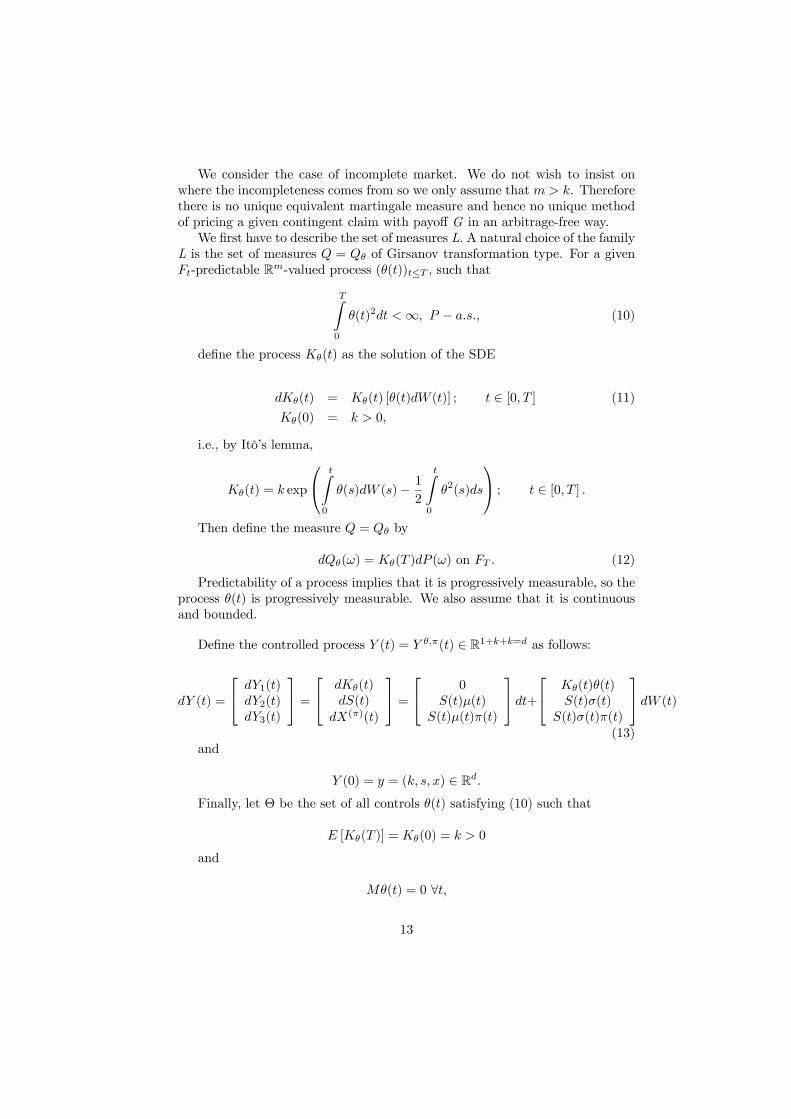
We consider the case of incomplete market. We do not wish to insist onwhere the incompleteness comes from so we only assume that m > k. Thereforethere is no unique equivalent martingale measure and hence no unique methodof pricing a given contingent claim with payoff G in an arbitrage-free way.We first have to describe the set of measures L. A natural choice of the family
L is the set of measures Q = Qθ of Girsanov transformation type. For a givenFt-predictable Rm-valued process (θ(t))t≤T , such that
TZ0
θ(t)2dt <∞, P − a.s., (10)
define the process Kθ(t) as the solution of the SDE
dKθ(t) = Kθ(t) [θ(t)dW (t)] ; t ∈ [0, T ] (11)
Kθ(0) = k > 0,
i.e., by Itô’s lemma,
Kθ(t) = k exp
⎛⎝ tZ0
θ(s)dW (s)− 12
tZ0
θ2(s)ds
⎞⎠ ; t ∈ [0, T ] .
Then define the measure Q = Qθ by
dQθ(ω) = Kθ(T )dP (ω) on FT . (12)
Predictability of a process implies that it is progressively measurable, so theprocess θ(t) is progressively measurable. We also assume that it is continuousand bounded.
Define the controlled process Y (t) = Y θ,π(t) ∈ R1+k+k=d as follows:
dY (t) =
⎡⎣ dY1(t)dY2(t)dY3(t)
⎤⎦ =⎡⎣ dKθ(t)
dS(t)dX(π)(t)
⎤⎦ =⎡⎣ 0
S(t)μ(t)S(t)μ(t)π(t)
⎤⎦ dt+⎡⎣ Kθ(t)θ(t)
S(t)σ(t)S(t)σ(t)π(t)
⎤⎦ dW (t)
(13)and
Y (0) = y = (k, s, x) ∈ Rd.Finally, let Θ be the set of all controls θ(t) satisfying (10) such that
E [Kθ(T )] = Kθ(0) = k > 0
and
Mθ(t) = 0 ∀t,
13
where
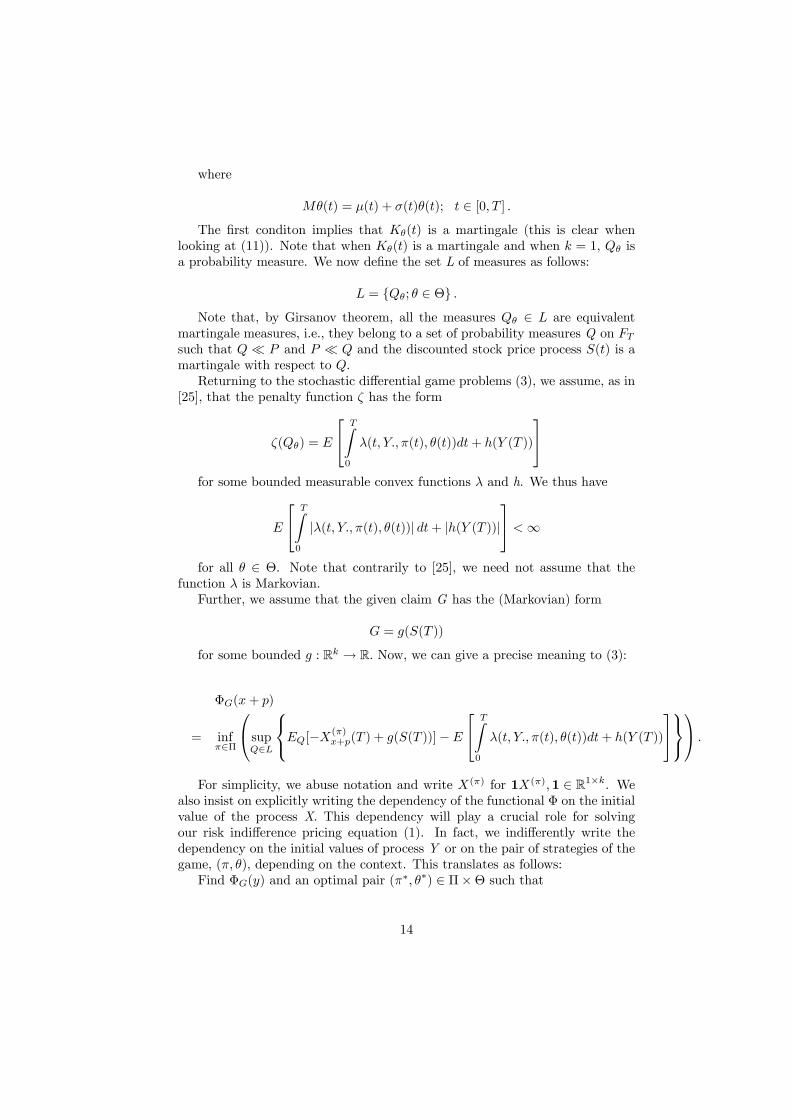
Mθ(t) = μ(t) + σ(t)θ(t); t ∈ [0, T ] .The first conditon implies that Kθ(t) is a martingale (this is clear when
looking at (11)). Note that when Kθ(t) is a martingale and when k = 1, Qθ isa probability measure. We now define the set L of measures as follows:
L = Qθ; θ ∈ Θ .Note that, by Girsanov theorem, all the measures Qθ ∈ L are equivalent
martingale measures, i.e., they belong to a set of probability measures Q on FTsuch that Q ¿ P and P ¿ Q and the discounted stock price process S(t) is amartingale with respect to Q.Returning to the stochastic differential game problems (3), we assume, as in
[25], that the penalty function ζ has the form
ζ(Qθ) = E
⎡⎣ TZ0
λ(t, Y., π(t), θ(t))dt+ h(Y (T ))
⎤⎦for some bounded measurable convex functions λ and h. We thus have
E
⎡⎣ TZ0
|λ(t, Y., π(t), θ(t))| dt+ |h(Y (T ))|
⎤⎦ <∞
for all θ ∈ Θ. Note that contrarily to [25], we need not assume that thefunction λ is Markovian.Further, we assume that the given claim G has the (Markovian) form
G = g(S(T ))
for some bounded g : Rk → R. Now, we can give a precise meaning to (3):
ΦG(x+ p)
= infπ∈Π
⎛⎝supQ∈L
⎧⎨⎩EQ[−X(π)x+p(T ) + g(S(T ))]−E
⎡⎣ TZ0
λ(t, Y., π(t), θ(t))dt+ h(Y (T ))
⎤⎦⎫⎬⎭⎞⎠ .
For simplicity, we abuse notation and write X(π) for 1X(π),1 ∈ R1×k. Wealso insist on explicitly writing the dependency of the functional Φ on the initialvalue of the process X. This dependency will play a crucial role for solvingour risk indifference pricing equation (1). In fact, we indifferently write thedependency on the initial values of process Y or on the pair of strategies of thegame, (π, θ), depending on the context. This translates as follows:Find ΦG(y) and an optimal pair (π∗, θ
∗) ∈ Π×Θ such that
14

ΦG(y) = ΦG(k, s, x) := infπ∈Π
µsupθ∈Θ
Jπ,θ(y)
¶= Jπ
∗,θ∗(y), (14)
where
Jπ,θ(y) = J(π, θ) := Ey
⎡⎣− TZ0
λ(t, Y., π(t), θ(t))dt− h(Y (T ))−Kθ(T )X(π)x (T ) +Kθ(T )g(S(T ))
⎤⎦ .The expectation on the right-hand side of the equation is the expectation
with respect to the probability law of Y (t) starting at y, i.e., where Y (0) = y.
4.2 Solution of the game
We now proceed as above in order to solve the stochastic differential zero-sumgame problem (14). Remember that the dynamics of the system is described by(13), which we abbreviate as follows:
dY (t) = f(t, Y., πt, θt)dt+ η(t, Y., πt, θt)dW (t). (15)
Contrarily to classical stochastic differential zero-sum game problems, thefunction η in (15) depends on the controls π and θ so the interpretation of theproblem will be different. Since we are not in the same setting as in Section 3.2we first present the (slightly weaker) assumptions on the coefficients in (15) forgeneral f and η and then check that the assumptions on the coefficients of (13)satisfy these conditions.Since the Hamiltonian of the game is much simpler here than in classical
stochastic differential zero-sum game problems, we can relax some assumptionson η, in particular, the fact that it is a square invertible matrix. So, η must bea function from [0, T ]× C × U × V into Rd×3m such that
• η is D-mesurable.
• ∀t ∈ [0, T ], ∀w,w0 ∈ C, there exists a constant k such that |η(t, w)− η(t, w0)| ≤k kw − w0kt .
• ∀t ∈ [0, T ], ∀w ∈ C, there exists a constant k such that |η(t, w)| ≤ k(1 +kw0kt).
Further, f must be a function from [0, T ]× C × U × V into Rd such that
• ∀(u, v) ∈ U×V, the mapping (t, w)→ f(t, w, u, v) is D-mesurable.
• ∀t ∈ [0, T ],∀w ∈ C, the mapping (u, v) → f(t, w, u, v) is continuous onU × V.
• f is bounded.
15
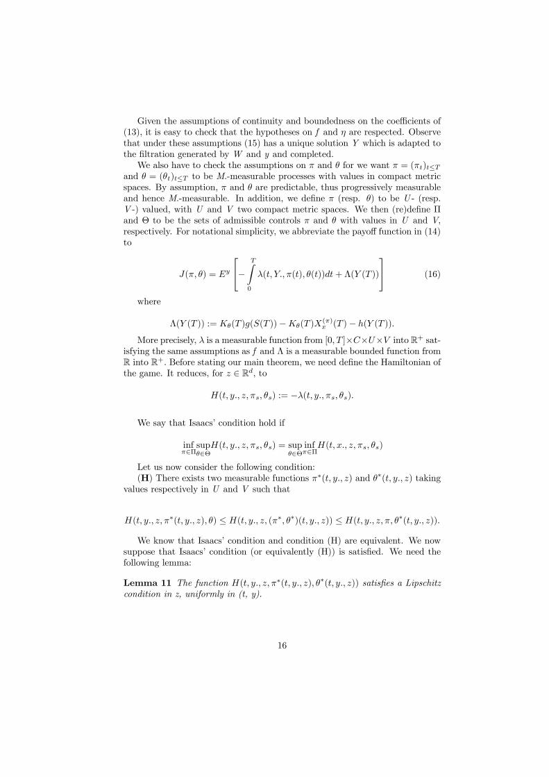
Given the assumptions of continuity and boundedness on the coefficients of(13), it is easy to check that the hypotheses on f and η are respected. Observethat under these assumptions (15) has a unique solution Y which is adapted tothe filtration generated by W and y and completed.We also have to check the assumptions on π and θ for we want π = (πt)t≤T
and θ = (θt)t≤T to be M.-measurable processes with values in compact metricspaces. By assumption, π and θ are predictable, thus progressively measurableand hence M.-measurable. In addition, we define π (resp. θ) to be U - (resp.V -) valued, with U and V two compact metric spaces. We then (re)define Πand Θ to be the sets of admissible controls π and θ with values in U and V,respectively. For notational simplicity, we abbreviate the payoff function in (14)to
J(π, θ) = Ey
⎡⎣− TZ0
λ(t, Y., π(t), θ(t))dt+ Λ(Y (T ))
⎤⎦ (16)
where
Λ(Y (T )) := Kθ(T )g(S(T ))−Kθ(T )X(π)x (T )− h(Y (T )).
More precisely, λ is a measurable function from [0, T ]×C×U×V into R+ sat-isfying the same assumptions as f and Λ is a measurable bounded function fromR into R+. Before stating our main theorem, we need define the Hamiltonian ofthe game. It reduces, for z ∈ Rd, to
H(t, y., z, πs, θs) := −λ(t, y., πs, θs).
We say that Isaacs’ condition hold if
infπ∈Π
supθ∈Θ
H(t, y., z, πs, θs) = supθ∈Θ
infπ∈Π
H(t, x., z, πs, θs)
Let us now consider the following condition:(H) There exists two measurable functions π∗(t, y., z) and θ∗(t, y., z) taking
values respectively in U and V such that
H(t, y., z, π∗(t, y., z), θ) ≤ H(t, y., z, (π∗, θ∗)(t, y., z)) ≤ H(t, y., z, π, θ∗(t, y., z)).
We know that Isaacs’ condition and condition (H) are equivalent. We nowsuppose that Isaacs’ condition (or equivalently (H)) is satisfied. We need thefollowing lemma:
Lemma 11 The function H(t, y., z, π∗(t, y., z), θ∗(t, y., z)) satisfies a Lipschitzcondition in z, uniformly in (t, y).
16
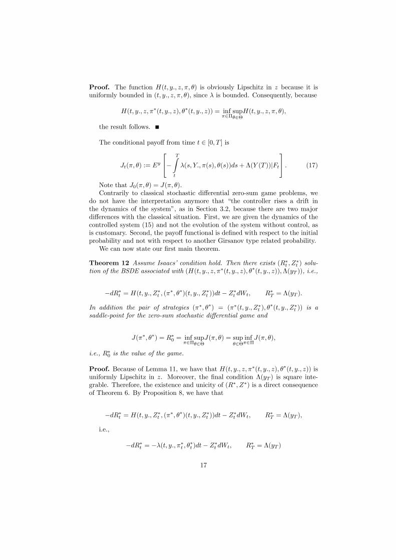
Proof. The function H(t, y., z, π, θ) is obviously Lipschitz in z because it isuniformly bounded in (t, y., z, π, θ), since λ is bounded. Consequently, because
H(t, y., z, π∗(t, y., z), θ∗(t, y., z)) = infπ∈Π
supθ∈Θ
H(t, y., z, π, θ),
the result follows.
The conditional payoff from time t ∈ [0, T ] is
Jt(π, θ) := Ey
⎡⎣− TZt
λ(s, Y., π(s), θ(s))ds+ Λ(Y (T ))|Ft
⎤⎦ . (17)
Note that J0(π, θ) = J(π, θ).Contrarily to classical stochastic differential zero-sum game problems, we
do not have the interpretation anymore that “the controller rises a drift inthe dynamics of the system”, as in Section 3.2, because there are two majordifferences with the classical situation. First, we are given the dynamics of thecontrolled system (15) and not the evolution of the system without control, asis customary. Second, the payoff functional is defined with respect to the initialprobability and not with respect to another Girsanov type related probability.We can now state our first main theorem.
Theorem 12 Assume Isaacs’ condition hold. Then there exists (R∗t , Z∗t ) solu-tion of the BSDE associated with (H(t, y., z, π∗(t, y., z), θ∗(t, y., z)),Λ(yT )), i.e.,
−dR∗t = H(t, y., Z∗t , (π∗, θ∗)(t, y., Z∗t ))dt− Z∗t dWt, R∗T = Λ(yT ).
In addition the pair of strategies (π∗, θ∗) = (π∗(t, y., Z∗t ), θ∗(t, y., Z∗t )) is a
saddle-point for the zero-sum stochastic differential game and
J(π∗, θ∗) = R∗0 = infπ∈Π
supθ∈Θ
J(π, θ) = supθ∈Θ
infπ∈Π
J(π, θ),
i.e., R∗0 is the value of the game.
Proof. Because of Lemma 11, we have that H(t, y., z, π∗(t, y., z), θ∗(t, y., z)) isuniformly Lipschitz in z. Moreover, the final condition Λ(yT ) is square inte-grable. Therefore, the existence and unicity of (R∗, Z∗) is a direct consequenceof Theorem 6. By Proposition 8, we have that
−dR∗t = H(t, y., Z∗t , (π∗, θ∗)(t, y., Z∗t ))dt− Z∗t dWt, R∗T = Λ(yT ),
i.e.,
−dR∗t = −λ(t, y., π∗t , θ∗t )dt− Z∗t dWt, R∗T = Λ(yT )
17
has a unique solution (R∗t , Z∗t ) ∈ S21(0, T ) × H2
d(0, T ) and R∗t is explicitlygiven by
R∗t = E
⎡⎣Λ(yT )Γt,T − TZt
Γt,sλ(s, y., π∗s, θ∗s)ds|Ft
⎤⎦where (Γt,s)s≥t is the adjoint process defined by the forward linear SDE
dΓt,s = 0, Γt,t = 1.
Therefore, Γt,s = 1 ∀t ≤ s ≤ T and
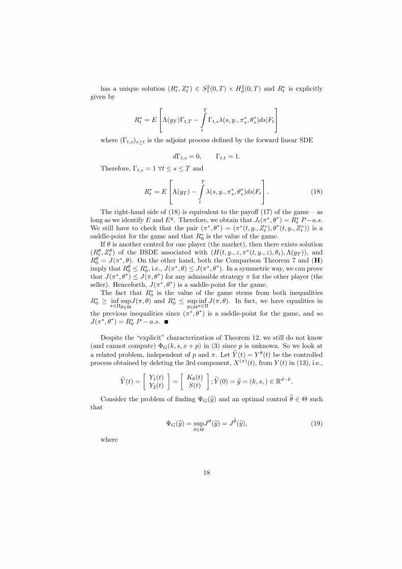
R∗t = E
⎡⎣Λ(yT )− TZt
λ(s, y., π∗s, θ∗s)ds|Ft
⎤⎦ . (18)
The right-hand side of (18) is equivalent to the payoff (17) of the game — aslong as we identify E and Ey. Therefore, we obtain that Jt(π∗, θ
∗) = R∗t P−a.s.We still have to check that the pair (π∗, θ∗) = (π∗(t, y., Z∗t ), θ
∗(t, y., Z∗t )) is asaddle-point for the game and that R∗0 is the value of the game.If θ is another control for one player (the market), then there exists solution
(Rθt , Z
θt ) of the BSDE associated with (H(t, y., z, π∗(t, y., z), θt),Λ(yT )), and
Rθ0 = J(π∗, θ). On the other hand, both the Comparison Theorem 7 and (H)
imply that Rθ0 ≤ R∗0, i.e., J(π
∗, θ) ≤ J(π∗, θ∗). In a symmetric way, we can provethat J(π∗, θ∗) ≤ J(π, θ∗) for any admissible strategy π for the other player (theseller). Henceforth, J(π∗, θ∗) is a saddle-point for the game.The fact that R∗0 is the value of the game stems from both inequalities
R∗0 ≥ infπ∈Π
supθ∈Θ
J(π, θ) and R∗0 ≤ supθ∈Θ
infπ∈Π
J(π, θ). In fact, we have equalities in
the previous inequalities since (π∗, θ∗) is a saddle-point for the game, and soJ(π∗, θ∗) = R∗0 P − a.s.
Despite the “explicit” characterization of Theorem 12, we still do not know(and cannot compute) ΦG(k, s, x+ p) in (3) since p is unknown. So we look ata related problem, independent of p and π. Let eY (t) = Y θ(t) be the controlledprocess obtained by deleting the 3rd component, X(π)(t), from Y (t) in (13), i.e.,
eY (t) = ∙ Y1(t)Y2(t)
¸=
∙Kθ(t)S(t)
¸; eY (0) = ey = (k, s, ) ∈ Rd−k.
Consider the problem of finding ΨG(ey) and an optimal control bθ ∈ Θ suchthat
ΨG(ey) = supθ∈Θ
Jθ(ey) = Jbθ(ey), (19)
where
18
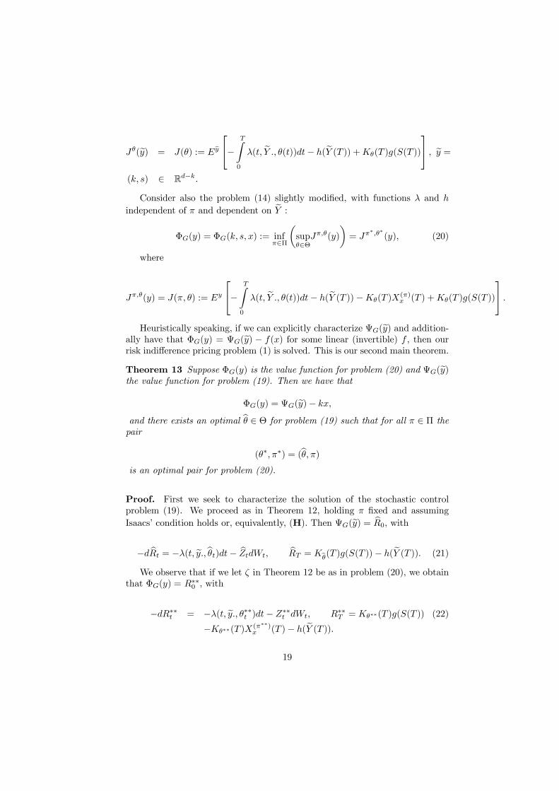
Jθ(ey) = J(θ) := Eey⎡⎣− TZ
0
λ(t, eY ., θ(t))dt− h(eY (T )) +Kθ(T )g(S(T ))
⎤⎦ , ey =(k, s) ∈ Rd−k.
Consider also the problem (14) slightly modified, with functions λ and h
independent of π and dependent on eY :ΦG(y) = ΦG(k, s, x) := inf
π∈Π
µsupθ∈Θ
Jπ,θ(y)
¶= Jπ
∗,θ∗(y), (20)
where
Jπ,θ(y) = J(π, θ) := Ey
⎡⎣− TZ0
λ(t, eY ., θ(t))dt− h(eY (T ))−Kθ(T )X(π)x (T ) +Kθ(T )g(S(T ))
⎤⎦ .Heuristically speaking, if we can explicitly characterize ΨG(ey) and addition-
ally have that ΦG(y) = ΨG(ey) − f(x) for some linear (invertible) f , then ourrisk indifference pricing problem (1) is solved. This is our second main theorem.
Theorem 13 Suppose ΦG(y) is the value function for problem (20) and ΨG(ey)the value function for problem (19). Then we have that
ΦG(y) = ΨG(ey)− kx,
and there exists an optimal bθ ∈ Θ for problem (19) such that for all π ∈ Π thepair
(θ∗, π∗) = (bθ, π)is an optimal pair for problem (20).
Proof. First we seek to characterize the solution of the stochastic controlproblem (19). We proceed as in Theorem 12, holding π fixed and assumingIsaacs’ condition holds or, equivalently, (H). Then ΨG(ey) = bR0, with−d bRt = −λ(t, ey.,bθt)dt− bZtdWt, bRT = Kbθ(T )g(S(T ))− h(eY (T )). (21)
We observe that if we let ζ in Theorem 12 be as in problem (20), we obtainthat ΦG(y) = R∗∗0 , with
−dR∗∗t = −λ(t, ey., θ∗∗t )dt− Z∗∗t dWt, R∗∗T = Kθ∗∗(T )g(S(T )) (22)
−Kθ∗∗(T )X(π∗∗)x (T )− h(eY (T )).
19

We can choose θ∗∗t = bθt in order to satisfy Isaacs’ condition, because λ isindependent of π both in (21) and (22). Note that for all π ∈ Π
EyhKbθ(T )X(π)
x (T )|Fti= EQbθ
hX(π)x (T )|Ft
iEy£Kbθ(T )|Ft¤ = X(π)
x (t)Kbθ(t)since Qbθ is an equivalent martingale measure and Kbθ(t) is a martingale. In
particular, when t = 0,
EyhKbθ(T )X(π)
x (T )|F0i= kx.
We also have
EyhKbθ(T )X(π)
x (T )i= kE 1
kQbθhX(π)x (T )
i= kx,
since 1kQbθ is an equivalent martingale measure as well. Comparing (21) and
(22), we see that R∗∗T = bRT −Kbθ(T )X(π∗∗)x (T ). Rewriting these (linear) BSDEs
as conditional expectations, as in the proof of Theorem 12, we then have
Jt(π∗, θ∗) = R∗∗t
= Ey
⎡⎣− TZt
λ(s, eY ., θ∗∗(s))ds− h(eY (T ))−Kθ∗∗(T )X(π∗∗)x (T ) +Kθ∗∗(T )g(S(T ))|Ft
⎤⎦= Ey
⎡⎣− TZt
λ(s, eY .,bθ(s))ds− h(eY (T )) +Kbθ(T )g(S(T ))|Ft⎤⎦−Kbθ(t)X(π∗∗)
x (t)
= bRt −Kbθ(t)X(π∗∗)x (t)
= Jt(bθ)−Kbθ(t)X(π∗∗)x (t).
When t = 0, we conclude that
ΦG(y) = ΨG(ey)− kx.
We also have that
J(π∗, θ∗) = J(bθ)− kx = J(π,bθ),so for all π ∈ Π the pair
(θ∗, π∗) = (bθ, π) ∈ Θ×Πis an optimal pair for problem (20), as claimed.
20
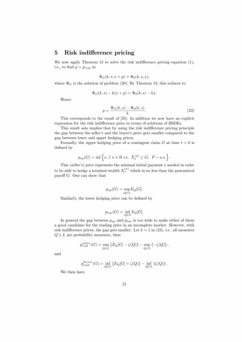
5 Risk indifference pricingWe now apply Theorem 13 to solve the risk indifference pricing equation (1),i.e., to find p = prisk in
ΦG(k, s, x+ p) = Φ0(k, s, x),
where ΦG is the solution of problem (20). By Theorem 13, this reduces to
ΨG(k, s)− k(x+ p) = Ψ0(k, s)− kx.
Hence
p =ΨG(k, s)−Ψ0(k, s)
k. (23)
This corresponds to the result of [25]. In addition we now have an explicitexpression for the risk indifference price in terms of solutions of BSDEs.This result aslo implies that by using the risk indifference pricing principle
the gap between the seller’s and the buyer’s price gets smaller compared to thegap between lower and upper hedging prices.Formally, the upper hedging price of a contingent claim G at time t = 0 is
defined by
pup(G) = infnx,∃ π ∈ Π s.t. X(π)
x ≥ G, P − a.s.o.
This (seller’s) price represents the minimal initial payment x needed in orderto be able to hedge a terminal wealth X(π)
x which in no less than the guaranteedpayoff G. One can show that
pup(G) = supQ∈L
EQ[G].
Similarly, the lower hedging price can be defined by
plow(G) = infQ∈L
EQ[G].
In general the gap between pup and plow is too wide to make either of thema good candidate for the trading price in an incomplete market. However, withrisk indifference prices, the gap gets smaller. Let k = 1 in (23), i.e., all measuresQ ∈ L are probability measures, then
psellerrisk (G) = supQ∈L
EQ[G]− ζ(Q)− supQ∈L
−ζ(Q) ,
and
pbu yerrisk (G) = infQ∈L
EQ[G] + ζ(Q)− infQ∈L
ζ(Q) .
We then have
21
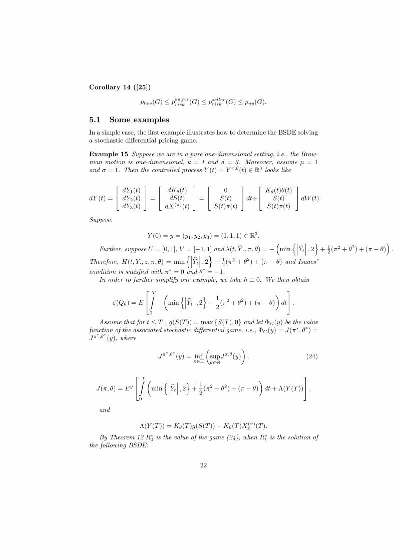
Corollary 14 ([25])
plow(G) ≤ pbu yerrisk (G) ≤ psellerrisk (G) ≤ pup(G).
5.1 Some examples
In a simple case, the first example illustrates how to determine the BSDE solvinga stochastic differential pricing game.
Example 15 Suppose we are in a pure one-dimensional setting, i.e., the Brow-nian motion is one-dimensional, k = 1 and d = 3. Moreover, assume μ = 1and σ = 1. Then the controlled process Y (t) = Y π,θ(t) ∈ R3 looks like
dY (t) =
⎡⎣ dY1(t)dY2(t)dY3(t)
⎤⎦ =⎡⎣ dKθ(t)
dS(t)dX(π)(t)
⎤⎦ =⎡⎣ 0
S(t)S(t)π(t)
⎤⎦ dt+⎡⎣ Kθ(t)θ(t)
S(t)S(t)π(t)
⎤⎦ dW (t).Suppose
Y (0) = y = (y1, y2, y3) = (1, 1, 1) ∈ R3.
Further, suppose U = [0, 1], V = [−1, 1] and λ(t, eY ., π, θ) = −³minn¯eYt ¯ , 2o+ 12(π
2 + θ2) + (π − θ)´.
Therefore, H(t, Y., z, π, θ) = minn¯eYt ¯ , 2o + 1
2(π2 + θ2) + (π − θ) and Isaacs’
condition is satisfied with π∗ = 0 and θ∗ = −1.In order to further simplify our example, we take h ≡ 0. We then obtain
ζ(Qθ) = E
⎡⎣ TZ0
−µmin
n¯eYt ¯ , 2o+ 12(π2 + θ2) + (π − θ)
¶dt
⎤⎦ .Assume that for t ≤ T , g(S(T )) = max S(T ), 0 and let ΦG(y) be the value
function of the associated stochastic differential game, i.e., ΦG(y) = J(π∗, θ∗) =Jπ∗,θ∗(y), where
Jπ∗,θ∗(y) = inf
π∈Π
µsupθ∈Θ
Jπ,θ(y)
¶, (24)
J(π, θ) = Ey
⎡⎣ TZ0
µmin
n¯eYt ¯ , 2o+ 12(π2 + θ2) + (π − θ)
¶dt+ Λ(Y (T ))
⎤⎦ ,and
Λ(Y (T )) = Kθ(T )g(S(T ))−Kθ(T )X(π)x (T ).
By Theorem 12 R∗0 is the value of the game (24), when R∗t is the solution ofthe following BSDE:
22

−dR∗t =µmin
n¯eYt ¯ , 2o+ 32
¶dt− Z∗t dWt, R∗T = Λ(YT ).
Now, R∗0 can be evaluated numerically ([6];[22];[30]).
The second example shows how an explicit formula for a risk indifferenceprice can be deduced from Example 15.
Example 16 Consider the same setting as in the preceding example. Let
eY (t) = ∙ Y1(t)Y2(t)
¸=
∙Kθ(t)S(t)
¸; eY (0) = ey = (1, 1) ∈ R2.
Consider the problem of finding ΨG(ey) and an optimal control bθ ∈ Θ such thatΨG(ey) = sup
θ∈ΘJθ(ey) = J
bθ(ey), (25)
where
Jθ(ey) := Ey
⎡⎣ TZ0
µmin
n¯eYt ¯ , 2o+ 12(π2 + θ2) + (π − θ)
¶dt+Kθ(T )g(S(T ))
⎤⎦ ,ey = (1, 1) ∈ R2.
We have that bR0 is the value of the game (25), bRt being the solution of thefollowing BSDE:
−d bRt =
µmin
n¯eYt ¯ , 2o+ 32
¶dt− bZtdWt, bRT = Kbθ(T )g(S(T )). (26)
Now applying Theorem 13 we have that
ΦG(y) = ΨG(ey)− kx.
Our risk indifference pricing equation (1) then becomes
ΦG(1, 1, 1 + p) = Φ0(1, 1, 1),
which reduces to
ΨG(1, 1)− p = Ψ0(1, 1).
Hence
p = ΨG(1, 1)−Ψ0(1, 1),where Ψ0(1, 1) is the solution of a BSDE similar to (26) but with terminal valueequal to zero.
23
6 Markovian BSDEs and PDEsIn order to relate the BSDE solving the stochastic differential zero-sum gamein Theorem 12 to a PDE we consider the Markovian case, i.e., when the controlprocess Y (t) in (15) becomes
dY (t) = f(t, Yt, πt, θt)dt+ η(t, Yt, πt, θt)dW (t), Y (0) = y ∈ Rd
and when the payoff function in (16) becomes
Ey
⎡⎣− TZ0
λ(t, Y (t), π(t), θ(t))dt+ Λ(Y (T ))
⎤⎦ .Our BSDE then looks like
−dRyt = −λ(t, Yt, π∗t , θ∗t )dt− Zy
t dWt, RyT = Λ(YT ). (27)
We know from the non-linear Feynamn-Kac’s formula for semilinear PDEs([10]) that if (Ry
t , Zyt ) is the unique solution of (27), then u(t, y) := Ry
t , 0 ≤t ≤ T, y ∈ Rd belongs to C1,2
¡[0, T ]×Rd,R
¢and is a classical solution of the
following PDE:
(∂t + P )ut − λ(t, y, π∗t , θ∗t ) = 0,∀t ∈ [0, T ] , y ∈ Rd (28)
u(T, y) = Λ(y),∀y ∈ Rd,
where P is a second order partial differential operator given by
P :=1
2
Xi,j
(ηη)i,j∂2
∂xi∂xj+Xi
fi∂
∂xi
and where η is the transpose of η. As we expect, (28) corresponds to theresult in [14] (Chapter 17, Section 2), which uses existence results and properties(maximum principle) of parabolic partial differential equations in order to solvethe same stochastic differential game — except that [14] works in a boundeddomain of Rd, with smooth boundary. From a financial point of view, such aPDE approach could also lead to very tractable results.
7 ConclusionWe have managed to characterize the solution to a risk indifference pricingproblem by means of BSDEs solving zero-sum stochastic differential games.In [25], the same problem has been tackled using stochastic control meth-
ods and partial differential equations, namely Hamilton-Jacobi-Bellman-Isaacsequations for two player stochastic differential games.
24
Our (stochastic analysis) approach is more general in the sense that it doesnot impose Markovian assumptions on the coefficients — it is a well-known benefitof BSDEs over PDE techniques. It also encompasses the multi-dimensional case.Finally, it gives an explicit formula for the risk indifference price that can beeasily implemented numerically by means of Monte Carlo simulation.However, we have restrained ourselves to the diffusion case, whereas papers
using analytical techniques encompass the jump diffusion case ([23];[25]).Therefore, a direct area of improvement is to extend our approach to the
jump diffusion case. The task requires, although, proving new results in the the-ory of BSDEs, in particular in a non-continuous context, characterizing stochas-tic differential zero-sum games by BSDE with jumps. Then, these results couldpresumably be used to find the solution of risk indifference pricing problems inthe jump case.Concerning the connection with the work of [14] on stochastic differential
games, it would be interesting, in the non-continuous (jump) case, to furtherinvestigate the link between BSDEs with jumps, stochastic differential gamesand parabolic partial integro-differential equations, which could also be used tosolve risk indifference pricing problems.
References[1] Acerbi, C. and D. Tasche, 2002. On the coherence of expected shortfall.
In Szegö, G. (ed.). Beyond VaR (Special issue). Journal of Banking andFinance 26.
[2] Ankirchner, S., Imkeller, P. and G. Reis, 2007. Pricing and hedging ofderivatives based on non-tradable underlyings. Preprint.
[3] Artzner, P., Delbaen, F., Eber, J.-M. and D. Heath, 1999. Coherent mea-sures of risk. Mathematical Finance 9, 203-228.
[4] Barrieu, P. and N. El Karoui, 2005. Optimal derivative design under dy-namic risk measures. In Carmona, R. (ed.). Volume on indifference pricing,Princeton University Press.
[5] Benes, V.E., 1970. Existence of optimal strategies based on specified in-formation, for a class of stochastic decision problems. SIAM Journal ofControl, 8, 179-188.
[6] Bouchard, B. and N. Touzi, 2004. Discrete-time approximation and Monte-Carlo simulation of BSDEs. Stochastic Processes and their Applications,111 (2), 175-206.
[7] Delbaen, F., 2000. Coherent risk measures. Lectures notes at CattedraGalileiana at Scuola Normale di Pisa.
[8] Doege, J. and H.-J. Lüthi, 2005. Convex risk measures for portfolio opti-mization and concepts of flexibility. Working paper.
25
[9] El Karoui, N., Peng, S. and M.C. Quenez, 1997. Backward stochastic dif-ferential equations in finance. Mathematical Finance 7, 1-71.
[10] El Karoui, N., Hamadène, S. and A. Matoussi, 2005. Backward stochasticdifferential equations and applications. In Carmona, R. (ed.). Volume onindifference pricing, Princeton University Press.
[11] El Karoui, N. and S. Hamadène, 2003. BSDEs and risk-sensitive control,zero-sum and non-zero-sum game problems of stochastic functional differ-ential equations. Stochastic Processes and their Applications 107, 145-169.
[12] Elliott, R., 1976. The existence of value in stochastic differential games.SIAM Journal on Control and Optimization 14, 85-94.
[13] Föllmer, H. and A. Schied, 2002. Convex measures of risk and tradingconstraints. Finance and Stochastics 6, 429-447.
[14] Friedman, A., 1975. Stochastic differential equations and applications. Twovolumes bound as one. Dover Publications.
[15] Frittelli, M. and E.R. Gianin, 2002. Putting order in risk measures. Journalof Banking and Finance 26, 773-797.
[16] Hamadène, S., 2006. Mixed zero-sum stochastic differential game andAmerican game options. Siam Journal of Control and Optimization 45 (2),496-518.
[17] Hamadène, S. and J.P. Lepeltier, 1995. Zero-sum stochastic differentialgames and backward equations. Systems & Control Letters 24, 259-263.
[18] Henderson, V. and D. Hobson, 2005. Utility indifference pricing: Anoverview. In Carmona, R. (ed.). Volume on indifference pricing, Prince-ton University Press.
[19] Hodges, S. D. and A. Neuberger, 1989. Optimal replication of contingentclaim under transaction costs. Review of Future Markets 8, 222-239.
[20] Hu, Y., Imkeller, P. and M. Müller, 2005. Utility maximisation in incom-plete markets. Annals of Applied Probability 15 (3), 1691-1712.
[21] Karatzas, I. and S. Shreve, 1988. Brownian motion and stochastic calculus.Gradutate texts in mathematics, Springer Verlag.
[22] Labart, C., 2007. EDSR: analyse de discrétisation et résolution par méth-odes de Monte Carlo adaptatives ; Perturbations de domaines pour lesoptions américaines. Thèse de l’Ecole Polytechnique.
[23] Mataramvura, S. and B. Oksendal, 2007. Risk minimizing portfolios anHJBJ equations for stochastic differential games. Working paper.
26
[24] Musiela, M. and T. Zariphopolou, 2004. An example of indifference pricesunder exponential preferences. Finance and Stochastics 8, 229-239.
[25] Oksendal, B. and A. Sulem, 2008. Risk indifference pricing in jump diffusionmarkets. Mathematical Finance, to appear.
[26] Pardoux, E. and S. Peng, 1990. Adapted solutions of a backward stochasticdifferential equation. Systems and Control Letters 14, 55-61.
[27] Revuz, D. and M. Yor, 1994. Continuous martingales and Brownian motion.Grundlehren der mathematischen Wissenschaften 293, Springer Verlag, 2ndedition.
[28] Rockafellar, R.T and S. Uryasev, 2000. Conditional Value-at-Risk for gen-eral loss distributions. Journal of Banking and Finance 26, 1443-1471.
[29] Xu, M., 2005. Risk measure pricing and hedging in incomplete markets.Annals of Finance 2 (1), 51-71.
[30] Zhang J., 2004. A numerical scheme for BSDEs. Annals of Applied Proba-bility 14 (1), 459-488.
27