stochastic partial differential equations driven by l�vy space-time white noise

arX

iv:m

ath/

0407

131v

1 [

mat

h.PR

] 8

Jul

200

4

The Annals of Applied Probability

2004, Vol. 14, No. 3, 1506–1528DOI: 10.1214/105051604000000413c© Institute of Mathematical Statistics, 2004

STOCHASTIC PARTIAL DIFFERENTIAL EQUATIONS DRIVEN

BY LEVY SPACE-TIME WHITE NOISE

By Arne Løkka,1 Bernt Øksendal and Frank Proske

University of Oslo, Norwegian School of Economics and Business

Administration and University of Oslo, and University of Oslo

In this paper we develop a white noise framework for the studyof stochastic partial differential equations driven by a d-parameter(pure jump) Levy white noise. As an example we use this theory tosolve the stochastic Poisson equation with respect to Levy white noisefor any dimension d. The solution is a stochastic distribution processgiven explicitly. We also show that if d ≤ 3, then this solution canbe represented as a classical random field in L2(µ), where µ is theprobability law of the Levy process. The starting point of our theoryis a chaos expansion in terms of generalized Charlier polynomials.Based on this expansion we define Kondratiev spaces and the LevyHermite transform.

1. Introduction. White noise analysis has become a subject of muchcurrent interest. This theory was first treated by Hida [14] and extensivelystudied in many other works. See [16] and the references therein. Theseinvestigations are based on the concept of a Gaussian measure and the asso-ciated expansion into Hermite polynomials. Later on an extension of whitenoise theory to non-Gaussian analysis was established in [4] and developedfurther by Kondratiev, Da Silva, Streit and Us [24] and Kondratiev, Da Silvaand Streit [23]. The main tool of this theory is a biorthogonal decomposi-tion, which extends the Wiener–Ito chaos expansion. White noise analysishas been used in a broad range of applications. This approach was originallyapplied in quantum physics. See, for example, [3] or [2]. Subsequently, newapplications have been found in stochastic (partial) differential equations

Received November 2002; revised February 2003.1Supported by the Norwegian Research Council, Grant 134228/432.AMS 2000 subject classifications. 60G51, 60H40, 60H15.Key words and phrases. Levy processes, white noise analysis, stochastic partial differ-

ential equations.

This is an electronic reprint of the original article published by theInstitute of Mathematical Statistics in The Annals of Applied Probability,2004, Vol. 14, No. 3, 1506–1528. This reprint differs from the original inpagination and typographic detail.

1

http://arXiv.org/abs/math/0407131v1

http://www.imstat.org/aap/

http://dx.doi.org/10.1214/105051604000000413

http://www.imstat.org

http://www.ams.org/msc/

http://www.imstat.org

http://www.imstat.org/aap/

http://dx.doi.org/10.1214/105051604000000413

2 A. LØKKA, B. ØKSENDAL AND F. PROSKE

[17]. See also [21] and [6] to mention a few. More recently, the theory hasbeen applied to finance [1]. See [18] and [12] for the fractional Brownianmotion case and [10] and [34] in the non-Gaussian case.

The object of this paper is to provide a white noise framework, basedon results in [28, 10, 34] and [17], to study SPDEs driven by (pure jump)Levy processes. We apply this theory to solve the stochastic Poisson equation

driven by a d-parameter ( pure jump) Levy white noise. That is, consider thefollowing model for the temperature U(x) at point x in a bounded domainD in Rd. Suppose that the temperature at the boundary ∂D of D is keptequal to zero and that there is a random heat source in D modeled by Levy

white noise.

η(x) =.

η(x1, . . . , xd). Then U is described by the equation

∆U(x) = −.

η(x), x= (x1, . . . , xd) ∈DU(x) = 0, x ∈ ∂D.

(1.1)

It is natural to guess that the solution must be

U(x) =U(x,ω) =

∫

DG(x, y)dη(y),(1.2)

where G(x, y) is the classical Green function for D and the integral onthe right-hand side is a multiparameter Ito integral with respect to thed-parameter Levy process η(x). But the integral on the right-hand side of(1.2) only makes sense if G(x, ·) is square integrable in D with respect tothe Lebesgue measure. The latter is true if and only if the dimension d ischosen lower than 4. Despite this difficulty we will show the existence of aunique explicit solution

x 7→ U(x, ·) ∈ (S)−1,

where (S)−1 is a suitable space of stochastic distributions, called the Kon-dratiev space.

The stochastic Poisson equation (1.1) was discussed by Walsh [39] in thecase of Brownian white noise W . He proved that there exists for all d aSobolev space H−n(D) and an H−n(D)-valued stochastic process

U = U(ω) :Ω→H−n(D)

such that (1.1) holds in the sense of distributions, for example,

〈U(·, ω),∆φ〉 = −〈W (·, ω), φ〉 a.s. for all φ ∈H−n(D).

The solution of Walsh is given explicitly by

〈U,φ〉 =

∫

Rd

∫

RdG(x, y)φ(x)dxdB(y); φ ∈H−n(D).(1.3)

LEVY SPACE-TIME WHITE NOISE 3

The system (1.1) was also studied in [17] in the Gaussian case. There thesolution U(x), which takes values in the Kondratiev space, can be describedby its action on test functions f ∈ (S)1,

〈U(x), f〉=

∫

RdG(x, y)〈W (y), f〉dy; f ∈ (S)1.(1.4)

If we compare (1.3) and (1.4) we find that the Walsh solution takes x-averages for almost all ω, whereas the last one takes ω-averages for all x.

Our solution is an extension of (1.4) to Levy processes. The approach weuse to solve (1.1) is based on a chaos expansion in terms of generalized Char-lier polynomials (cf. [28]) and on concepts developed in [17, 10] and [34]. Ourmethod, which can be applied to other classes of SPDEs, has the advantagethat SPDEs can be interpreted in the usual strong sense with respect totime and space. There is no need for a weak distribution interpretation withrespect to time and space. Furthermore, the Walsh construction reveals thedisadvantage of defining a multiplication of (Sobolev or Schwartz) distribu-tions, if one considers SPDEs, where the noise is involved multiplicatively.However, on the Kondratiev space (S)−1 we can define a multiplication, theLevy Wick product. This gives a natural interpretation of SPDEs, wherethe noise or other terms appear multiplicatively. Furthermore, in some casessolutions can be explicitly obtained in terms of the Wick product. See [17].

The general machinery, developed in this paper, is of independent interestand we are convinced that it serves a useful tool for the study of a large classof stochastic partial differential equations driven by Levy space-time whitenoise.

Finally, let us mention that there has recently been an increasing interestin solving SPDEs driven by d-parameter Levy processes. We refer to [5, 29]and the references therein.

We shall give an overview of the paper. In Section 2 we introduce a whitenoise framework for the study of SPDEs driven by d-parameter Levy pro-cesses. The starting point of our theory is a chaos expansion in terms ofgeneralized Charlier polynomials. Based on this expansion we define Kon-dratiev spaces, the Wick product and the d-parameter Levy white noise.Further, we give the definition of the Levy Hermite transform and state acharacterization theorem for the Kondratiev space (S)−1. In Section 3 weuse the tools developed in Section 2 to apply it to solve the stochastic Pois-son equation driven by a d-parameter Levy white noise. Finally, in Section 4we discuss the solution and its properties. In particular, we show that ifd≤ 3, the solution can be represented as a classical random field in L2(µ),where µ is the underlying probability law of the Levy process.

2. Framework. In this section we give the general framework to be usedlater. The starting point for our discussion are white noise concepts for Levy


processes, developed in [10, 34] and [28]. Actually, we empasize the use ofmultidimensional structures, that is, the white noise we intend to consider isindexed by a multidimensional parameter set. Our presentation and notationwill follow that of [17] closely, where Gaussian white noise theory is treated.For more information about white noise theory we refer to [16, 26] and [32].

2.1. A white noise construction of Poisson random measures associated

with a Levy process. In this paper we confine ourselves to (d-parameter)pure jump Levy processes without drift.

A pure jump Levy process η(t) on R with no drift is a process with in-dependent and stationary increments, continuous in probability and withno Brownian motion part. The characteristic function of such a process isgiven by the Levy–Khintchine formula in terms of the Levy measure ν ofthe Levy process, that is, in terms of a measure ν on R0 := R − 0, thatintegrates the function 1 ∧ z2. Hence, driftless pure jump Levy processescan be characterized as Levy processes with characteristic triplet (0,0, ν).For general information about Levy processes see [8] and [36]. In general,such processes do not possess the chaotic representation property, but theyadmit a chaos representation with respect to Poisson random measures (see[19]). Therefore, we aim at viewing these processes as elements of a certainPoisson space. In this framework we will give a white noise construction ofPoisson random measures and, since our emphasis lies on processes indexedby multidimensional sets, we will define d-parameter (pure jump) Levy pro-cesses. Further, we prove a chaos expansion in terms of generalized Charlierpolynomials.

A usual starting point in white noise analysis is the application of theBochner–Minlos theorem to prove the existence of a probability measureon the space of tempered distributions S p(Rd). However, it turns out thatS p(Rd) is not the most appropriate for dealing with Levy processes sincethis choice would require restrictive conditions to be imposed on the Levymeasure. This circumstance comes from the fact that the Levy measure hasa singularity at zero. Therefore, we use the construction of a nuclear algebraS(X), which is more tractable for our purpose. In fact, the space S(X) is

a variant of the Schwartz space on X = Rd × R0, more precisely S(X) is a

subspace of the Schwartz space modulo a certain subspace depending on theLevy measure. Let us first give the construction of S(X) (cf. [28]).

In the following let ξnn≥0 be the complete orthogonal system of L2(R),consisting of the Hermite functions. Then the (countably Hilbertian) nucleartopology of the Schwartz space S(Rd) is induced by the compatible systemof norms

‖ϕ‖2γ :=

∑

α∈Nd

(1 +α)2γ(ϕ, ξα)2L2(Rd), γ ∈ Nd0,(2.1)


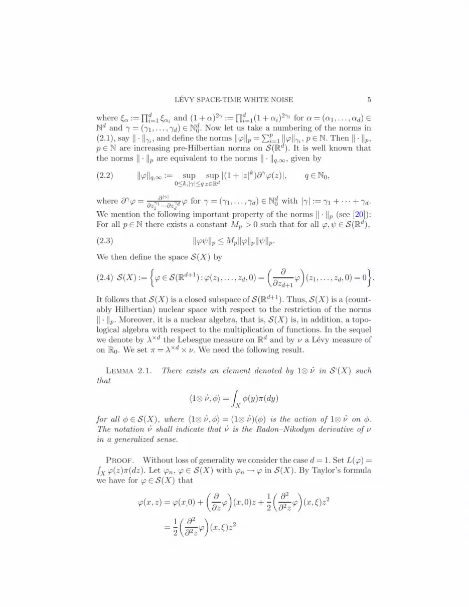
where ξα :=∏di=1 ξαi

and (1 +α)2γ :=∏di=1(1 +αi)

2γi for α= (α1, . . . , αd) ∈Nd and γ = (γ1, . . . , γd) ∈ Nd

0. Now let us take a numbering of the norms in(2.1), say ‖ · ‖γi

, and define the norms ‖ϕ‖p =∑pi=1 ‖ϕ‖γi

, p ∈ N. Then ‖ · ‖p,p ∈ N are increasing pre-Hilbertian norms on S(Rd). It is well known thatthe norms ‖ · ‖p are equivalent to the norms ‖ · ‖q,∞, given by

‖ϕ‖q,∞ := sup0≤k,|γ|≤q

supz∈Rd

|(1 + |z|k)∂γϕ(z)|, q ∈ N0,(2.2)

where ∂γϕ = ∂|γ|

∂zγ11 ···∂z

γdd

ϕ for γ = (γ1, . . . , γd) ∈ Nd0 with |γ| := γ1 + · · · + γd.

We mention the following important property of the norms ‖ · ‖p (see [20]):For all p ∈ N there exists a constant Mp > 0 such that for all ϕ,ψ ∈ S(Rd),

‖ϕψ‖p ≤Mp‖ϕ‖p‖ψ‖p.(2.3)

We then define the space S(X) by

S(X) :=

ϕ ∈ S(Rd+1) :ϕ(z1, . . . , zd,0) =

(∂

∂zd+1ϕ

)(z1, . . . , zd,0) = 0

.(2.4)

It follows that S(X) is a closed subspace of S(Rd+1). Thus, S(X) is a (count-ably Hilbertian) nuclear space with respect to the restriction of the norms‖ · ‖p. Moreover, it is a nuclear algebra, that is, S(X) is, in addition, a topo-logical algebra with respect to the multiplication of functions. In the sequelwe denote by λ×d the Lebesgue measure on R

d and by ν a Levy measure ofon R0. We set π = λ×d × ν. We need the following result.

Lemma 2.1. There exists an element denoted by 1⊗.

ν in S p(X) such

that

〈1⊗.

ν,φ〉 =

∫

Xφ(y)π(dy)

for all φ ∈ S(X), where 〈1⊗.

ν,φ〉 = (1⊗.

ν)(φ) is the action of 1⊗.

ν on φ.The notation

.

ν shall indicate that.

ν is the Radon–Nikodym derivative of νin a generalized sense.

Proof. Without loss of generality we consider the case d= 1. Set L(ϕ) =∫X ϕ(z)π(dz). Let ϕn, ϕ ∈ S(X) with ϕn → ϕ in S(X). By Taylor’s formula

we have for ϕ ∈ S(X) that

ϕ(x, z) = ϕ(x,0) +

(∂

∂zϕ

)(x,0)z +

1

2

(∂2

∂2zϕ

)(x, ξ)z2

=1

2

(∂2

∂2zϕ

)(x, ξ)z2


for a point ξ between 0 and z.We assume w.l.o.g. that the measure ν vanishesoutside of [−1,0) ∪ (0,1]. Therefore, it follows by (2.2) that

|L(ϕn −ϕ)| ≤∫

R

∫ 1

−1|ϕn(x, z)−ϕ(x, z)|ν(dz)λ(dx)

≤∫

R

∫ 1

−1

(1 + |x|2 + |z|2)|ϕn(x, z)− ϕ(x, z)|

z2

×z2

(1 + |x|2)ν(dz)λ(dx)

≤ ‖ϕn − ϕ‖2,∞

∫

R

1

(1 + |x|2)λ(dx)

∫ 1

−1z2ν(dz)

→ 0 for n→∞.

So the linear functional L is continuous on S(X).

Next define the space

Nπ := φ ∈ S(X) :‖φ‖L2(π) = 0.(2.5)

By the same arguments as in the proof of Lemma 2.1 it can be shown thatNπ is a closed subspace of S(X). Furthermore, one checks that it is a closed

ideal of S(X). Now we introduce the space S(X), which we use to constructthe white noise measure.

Definition 2.2. We define the space S(X) as follows,

S(X) = S(X)/Nπ.(2.6)

The space S(X) is a (countably Hilbertian) nuclear algebra with the com-patible system of norms

‖φ‖p,π := infψ∈Nπ

‖φ+ψ‖p, p ∈ N.(2.7)

See page 72 in [13]. Further, let S p(X) denote the topological dual of S(X).

We obtain the following corollary to Lemma 2.1:

Corollary 2.3. The functional L(φ) :=∫X φ(z)π(dz) satisfies the in-

equality

|L(φ)| ≤Mp‖φ‖p,π

for all p≥ p0, which yields the continuity of the functional L on S(X).


Theorem 2.4. There exists a unique probability measure µ on the Borel

sets of S p(X) with the following Poissonian characteristic functional with

intensity π such that for all φ ∈ S(X):∫

S p(X)ei〈ω,φ〉 dµ(ω) = exp

(∫

X(eiφ − 1)dπ

),(2.8)

where 〈ω,φ〉 = ω(φ) is the action of ω ∈ S p(X) on φ ∈ S(X). Moreover, there

exists a p0 ∈ N such that 1 ⊗ ν ∈ S−p0(X) and a natural number q0 > p0

such that the imbedding operator Sq0(X) → Sp0(X) is Hilbert–Schmidt and

µ(S−q0(X)) = 1. The space Sp(X) denotes the completion of S(X) with re-

spect to ‖ · ‖p,π and S−p(X) is the corresponding dual with norm ‖ · ‖−p,π.

Proof. Since |eiz − 1| ≤ |z|, the result follows from Corollary 2.3 andBochners theorem for conuclear spaces [13].

We call the probability measure µ on Ω = S p(X) in Theorem 2.4 Levy

white noise probability measure. It turns out that this measure satisfies thefirst condition of analyticity in the following sense (see [23]).

Lemma 2.5. The Levy white noise measure µ satisfies the first condition

of analyticity, that is, there exists ǫ > 0 and a p0 such that∫

S p(X)exp(ǫ‖ω‖−p0)dµ(ω)<∞.

Proof. The proof follows the argument of Lemma 3 in [38]. Introducethe moment functions of µ, which by a criterion of Cramer [9] can be ex-pressed by

Mn(φ) :=

∫

S p(X)〈ω,φ〉n dµ(ω) =

d

dtnL(tφ)

∣∣∣∣t=0

for every φ ∈ S(X), n ∈ N. Define the set

Λkn :=

(α1, . . . , αk) ∈ N

k :k∑

i=1

αi = n

.

Then we obtain the following expression for Mn:

Mn(φ) =n∑

k=1

n!

k!

∑

α∈Λkn

k∏

j=1

〈1⊗ ν, φαj 〉

αj !.(2.9)

We get for the number p0 in Theorem 2.4 that

|〈1⊗ ν, φ〉| ≤ ‖1⊗ ν‖−p0,π‖φ‖p0,π <∞.


Next relation (2.3) implies that for all p ∈ N there exists a constant Mp > 0

such that for all φ,ψ ∈ S(X),

‖φψ‖p,π ≤Mp‖φ‖p,π‖ψ‖p,π.(2.10)

Thus, we get that

|〈1⊗ ν, φαj 〉| ≤ ‖1⊗ ν‖−p0,π(Mp0)αj‖φ‖

αjp0,π,

if we choose Mp0 ≥ 1. So we deduce from (2.9) that

|Mn(φ)| ≤n∑

k=1

n!

k!

∑

α∈Λkn

k∏

j=1

‖1⊗ ν‖−p0,παj !

Cnp0‖φ‖np0,π

= Fn(‖1⊗ ν‖−p0,π)Cnp0‖φ‖

np0,π,

where Fn(x) is the nth moment of the Poisson distribution with intensityx and where Cp0 is a constant. Further, it is known that for a Poissondistribution with intensity x= ‖1⊗ ν‖−p0,π, there exists a constant Cx suchthat for all n ∈ N,

|Fn(‖1⊗ ν‖−p0,π)| ≤ n!Cn‖1⊗ν‖−p0,π.

Therefore, we get for a C > 0 that

|Mn(φ)| ≤ n!Cn‖φ‖np0,π.

The claimed result follows from Lemma 3 in [23].

Further, consider the function α defined by α(φ) = log(1 +ϕ)modNπ forφ = ϕ with ϕ(x) > −1. Note that α is holomorphic at zero and invertible.With the help of Lemma 2.5, it can be shown just as in [28] that there existsymmetric kernels Cn(ω) such that for all φ in an open neighborhood of zero

in S(X),

e(φ,ω) :=exp〈ω,α(φ)〉

Eµ[e〈ω,α(φ)〉]=∑

n≥0

1

n!〈Cn(ω), φ⊗n〉,(2.11)

where φ⊗n ∈ S(X)⊗n. The symbol S(X)⊗n denotes the nth completed sym-

metric tensor product of S(X) with itself. The elements of this space canbe seen as functions f ∈ S(Xn) modulo Nπ×n such that f = f(x1, . . . , xn)is symmetric with respect to the variables x1, . . . , xn ∈X. From (2.11) weconclude that the Cn are generalized Charlier polynomials (see [23]). Wehave that

〈Cn(ω), φ(n)〉 :φ(n) ∈ S(X)⊗n, n ∈ N0(2.12)


is a total set in L2(µ). Furthermore, for all n, m, φ(n) ∈ S(X)⊗n and ψ(m) ∈

S(X)⊗m the orthogonality relation∫

S p(X)〈Cn(ω), φ(n)〉〈Cm(ω), ψ(m)〉dµ(ω) = δn,mn!(φ(n), ψ(n))L2(Xn)(2.13)

holds. See [28].

Remark 2.6. It can be easily seen from (2.13) and the construction of

S(X) that the Levy white noise measure µ is nondegenerate in the followingsense (see [23]): Let F be a continuous polynomial, that is, F is of the

form F (ω) =∑Nn=1〈ω

⊗n, φ(n)〉 for ω ∈ S p(X), N ∈ N0 with φ(n) ∈ SC(X)⊗n

[complexification of S(X)⊗n]. If F = 0 µ-a.e., then F (ω) = 0 for all ω ∈

S p(X). We mention that this property is essential for the construction ofcertain test function and distribution spaces (see [23, 28]).

Next, for functions f :Xn → R define the symmetrization (f)∧ of f by

(f)∧(x1, . . . , xn) :=1

n!

∑

n

f(xσ1 , . . . , xσn)(2.14)

for all permutations σ of 1, . . . , n. Then a function f :Xn → R is symmet-

ric, if and only if f = f . Denote by L2(Xn, π×n) the space of all symmet-ric functions on Xn, which are square integrable with respect to π×n. Letfn ∈ L

2(Xn, π×n). Since S(X) is dense in L2(X,π) (cf. [28]), we can choose a

sequence f(i)n in S(X)⊗n with f

(i)n → fn in L2(Xn, π×n). Then (2.13) implies

the existence of a well defined 〈Cn(ω), fn〉 such that

〈Cn(ω), fn〉= limi〈Cn(ω), f (i)

n 〉 in L2(Xn, π×n).(2.15)

Since C1(ω) = ω − 1⊗ ν for all φ ∈ S(X) (see [28]), we get∫

S p(X)〈ω − 1⊗ ν, f〉2 dµ(ω) = ‖f‖2

L2(π).(2.16)

Further, if we define for Borelian Λ1 ⊂ Rd, Λ2 ⊂ R0 with π(Λ1 × Λ2) <∞the random measures

N(Λ1,Λ2) := 〈ω,χΛ1×Λ2〉 and(2.17)

N(Λ1,Λ2) := 〈ω− 1⊗ ν, χΛ1×Λ2〉,

we see from their characteristic functions that N is a Poisson random mea-sure and N is the corresponding compensated Poisson random measure. The


compensator of N(Λ1,Λ2) is given by π. Therefore, it is natural to define

the stochastic integral of φ ∈L2(π) with respect to N by∫

Xφ(x, z)N (dx, dz) := 〈ω − 1⊗ ν, φ〉.(2.18)

In particular, if we define

η(x) :=

∫

Xχ[0,x1]×···×[0,xd](x) · zN(dx, dz)

(2.19)for x= (x1, . . . , xd) ∈ Rd,

where [0, xi] is interpreted as [xi,0], if xi < 0 and where the Levy measureν is assumed to integrate z2, then η(x) has a version η(x), which is cadlagin each component xi. This follows with the help of (2.13). We call η(x)d-parameter Levy process or space-time Levy process.

We conclude this section with a chaos expansion result in terms of the gen-eralized Charlier polynomials Cn. The result is a consequence of (2.12) and (2.13).

Theorem 2.7. If F ∈ L2(µ), then there exists a unique sequence fn ∈

L2(Xn) such that

F (ω) =∑

n≥0

〈Cn(ω), fn〉.(2.20)

Moreover, we have the isometry

‖F‖2L2(µ) =

∑

n≥0

n!‖fn‖2L2(Xn).(2.21)

2.2. Chaos expansion, Kondratiev spaces (S)ρ, (S)−ρ and Levy white noise.

First we reformulate the chaos expansion of Theorem 2.7. Then we use thenew expansion to define a Wick product on spaces of stochastic test functionsand stochastic distributions. The definitions and results here are analogousto the one-parameter case, which is treated in [10] and [34].

From now on we suppose that our Levy measure ν satisfies the conditionof [30], namely, that for every ε > 0 there exists a λ > 0 such that

∫

R\(−ε,ε)exp(λ|z|)ν(dz)<∞.(2.22)

This implies that our Levy measure has finite moments of all orders ≥ 2.For later use we introduce multi-indices of arbitrary length. To simplify

the notation, we regard multi-indices as elements of the space (NN0 )c of all

sequences α= (α1, α2, . . . ) with elements αi ∈ N0 and with compact support,that is, with only finitely many αi 6= 0. We define

J = (NN0 )c.


Further, we set Index(α) = maxi :αi 6= 0 and |α| =∑iαi for α ∈ J .

Next we consider two families of orthogonal polynomials. We use thesepolynomials to reformulate the chaos expansion of Theorem 2.7. First letξkk≥1 be the Hermite functions, just as in Section 2.1. Now choose abijective map

h :Nd→ N.

Define the function ζk(x1, . . . , xd) = ξi1(x1) · · · ξid(xd), if k = h(i1, . . . , id) for ij ∈N. Then ζkk≥1 constitutes an orthonormal basis of L2(Rd).

Further, let lmm≥0 be the orthogonalization of 1, z, z2, . . . with re-spect to the innerproduct of L2(), where (dz) = z2ν(dz). Then define thepolynomials

pm(z) =1

‖lm−1‖L2(ρ)z · lm−1(z).(2.23)

The polynomials pm form a complete orthonormal system in L2(ν) (see[34]). We shall mention that we could also use any orthonormal basis inS(X) ⊂ L2(ν) for d = 0 instead of the polynomials pm. In this case theintegrability condition (2.22) reduces to the requirement of the existence ofthe second moment with respect to ν. The choice of the polynomials pmserves to ease notation.

Next define the bijective map

z :N× N → N; (i, j) 7→ j + (i+ j − 2)(i+ j − 1)/2.(2.24)

Note that z(i, j) gives the “Cantor diagonalization” of N ×N.Then, if k = z(i, j) for i, j ∈ N, let

δk(x, z) = ζi(x)pj(z).

Further, assume Index(α) = j and |α| =m for α ∈ J and identify the func-tion δ⊗α as

δ⊗α((x1, z1), . . . , (xm, zm))

= δ⊗α11 ⊗ · · · ⊗ δ

⊗αj

j ((x1, z1), . . . , (xm, zm))(2.25)

= δ1(x1, z1) · · · δ1(xα1 , zα1)

· · · δj(xα1+···+αj−1+1, zα1+···+αj−1+1) · · · δj(xm, zm),

where the terms with zero-components αi are set equal to 1 in the product(δ⊗0i = 1).Finally, we define the symmetrized tensor product of the δk’s, denoted by

δ⊗α as

δ⊗α((x1, z1), . . . , (xm, zm))

= (δ⊗α)∧((x1, z1), . . . , (xm, zm))(2.26)

= δ⊗α11 ⊗ · · · ⊗δ

⊗αj

j ((x1, z1), . . . , (xm, zm)).


For α ∈ J define

Kα(ω) := 〈C|α|(ω), δ⊗α〉,(2.27)

where we let K0(ω) = 1. For example, if α= ǫl with

ǫl(j) =

1, for j = l,0, else,

l≥ 1,(2.28)

we obtain

Kǫl(ω) = 〈ω, δ⊗ǫl

〉= 〈ω, δl〉 = 〈ω, ζi(x)pj(z)〉,(2.29)

if l= z(i, j).

By Theorem 2.7 any sequence of functions fm ∈ L2(π×m), m= 0,1,2, . . . ,such that

∑m≥1m!‖fm‖

2L2(π×m) <∞ defines a random variable F ∈ L2(µ)

by F (ω) =∑m≥0〈Cm(ω), fm〉. Since each fm is contained in the closure of

the linear span of the orthogonal family δ⊗α|α|=m in L2(π×m), we get forall m≥ 1 the representation

fm =∑

|α|=m

cαδ⊗α(2.30)

in L2(π×m) for cα ∈ R. Hence, we can restate Theorem 2.7 as follows.

Theorem 2.8. The family Kαα∈J constitutes an orthogonal basis for

L2(µ) with norm expression

‖Kα‖2L2(µ) = α! := α1!α2! · · · ,(2.31)

for α= (α1, α2, . . . ) ∈ J . Thus, every F ∈ L2(µ) has the unique representa-

tion

F =∑

α∈J

cαKα,(2.32)

where cα ∈ R for all α and where we set c0 =E[F ].Moreover, we have the isometry

‖F‖2L2(µ) =

∑

α∈J

α!c2α.(2.33)

Example 2.9. (i) Choose F (ω) = η(x), the d-parameter Levy process.

Then η(x) =∫[0,x1]×···×[0,xd]×R0

zN (dx, dz) = 〈ω,χ[0,x1]×···×[0,xd](x) ·z〉 a.e. and

it follows by (2.29) that

η(x) =∑

k≥1

m

∫ xd

0· · ·∫ x1

0ζk(x1, . . . , xd)dx1 · · · dxd ·Kǫz(k,1) ,(2.34)


where m= ‖x‖L2(ν).(ii) Let Λ1 ⊂ R

m, Λ2 ⊂ R0 with π(Λ1×Λ2)<∞. Set f1(x, z) = χΛ1×Λ2(x, z).

Then by (2.29) and (2.30) we get for F = N(Λ1,Λ2) = 〈ω,f1〉

N(t,Λ) =∑

k,m≥1

∫

Λ1

∫

Λ2

ζk(x)pm(z)ν(dz)dx ·Kǫz(k,m) .(2.35)

Next we define various generalized function spaces that relate to L2(µ) ina natural way. These spaces turn out to be a useful tool to study stochasticpartial differential equations. Our spaces are Levy versions of the Kondratievspaces, which were originally introduced in [22]. See also [4] and [25] in thecontext of Gaussian analysis. The one-parameter case with respect to theLevy white noise measure µ can be found in [10] and [34]. The extension tomultidimensional parameter sets is analogous.

Definition 2.10. (i) The stochastic test function spaces. Let 0≤ ρ≤ 1.For an expansion f =

∑α∈J cαKα ∈ L2(µ) define the norm

‖f‖2ρ,k :=

∑

α∈J

(α!)1+ρc2α(2N)kα(2.36)

for k ∈ N0, where (2N)kα = (2 · 1)kα1(2 · 2)kα2 · · · (2 ·m)kαm , if Index(α) =m.Let

(S)ρ,k := f :‖f‖ρ,k <∞

and define

(S)ρ :=⋂

k∈N0

(S)ρ,k,(2.37)

endowed with the projective topology.(ii) The stochastic distribution spaces. Let 0≤ ρ≤ 1. In the same manner,

define for a formal expansion F =∑α∈J bαKα the norms

‖F‖2−ρ,−k :=

∑

α∈J

(α!)1−ρc2α(2N)−kα, k ∈ N0.(2.38)

Set

(S)−ρ,−k := F : ‖F‖−ρ,−k <∞

and define

(S)−ρ :=⋃

k∈N0

(S)−ρ,−k,(2.39)

equipped with the inductive topology.


We can regard (S)−ρ as the dual of (S)ρ by the action

〈F,f〉=∑

α∈J

bαcαα!(2.40)

for F =∑α∈J bαKα ∈ (S)−ρ and f =

∑α∈J bαKα ∈ (S)ρ. Note that for

general 0≤ ρ≤ 1 we have

(S)1 ⊂ (S)ρ ⊂ (S)0 ⊂L2(µ)⊂ (S)−0 ⊂ (S)−ρ ⊂ (S)−1.(2.41)

The space (S) := (S)0, respectively, (S)∗ := (S)−0, is a Levy version of theHida test function space, respectively, Hida stochastic distribution space.

For more information about these or related spaces in the Gaussian andPoissonian case we refer to [16] and [17].

One of the remarkable properties of the space (S)∗ is that it accomodatesthe (d-parameter) Levy white noise. See [10].

Definition 2.11. The (d-parameter) Levy white noise.

η(x) of the Levyprocess η(x) (with m= ‖z‖L2(ν)) is defined by the formal expansion

.

η(x) =m∑

k≥1

ζk(x)Kǫz(k,1) ,(2.42)

where ζk(x) is defined by Hermite functions, z(i, j) is the map in (2.24) andwhere ǫl ∈ J is defined as in (2.28).

Remark 2.12. (i) Because of the uniform boundedness of the Hermite

functions (see, e.g., [37]) the Levy white noise.

η(x) takes values in (S)∗ forall x. Further, it follows from (2.34) that

∂d

∂x1 · · ·∂xdη(x) =

.

η(x) in (S)∗.(2.43)

This justifies the name white noise for.

η(x).

(ii) Just as in [34] the (d-parameter) white noise.

N (x, z) of the Poisson

random measure N(dx, dz) can be defined by.

N (x, z) =∑

k,m≥1

ζk(x)pm(z) ·Kǫz(k,m) ,(2.44)

where pm(z) are the polynomials from (2.23). We have that.

N (x, z) is con-

tained in (S)∗π-a.e. The relation (2.35) admits the interpretation of.

N (x, z)as a Radon–Nikodym derivative, that is, (formally)

.

N (x, z) =N(dx, dz)

dx× ν(dz)in (S)∗.(2.45)


The last relation entitles us to call.

N(x, z) white noise.

Moreover,.

η(x) is related to.

N(x, z) by

.

η(x) =

∫

R

z.

N (x, z)ν(dz).(2.46)

The relation above is given in terms of a Bochner integral with respect to ν(see [34]).

2.3. Wick product and Hermite transform. In this section we define a(stochastic) Wick product on the space (S)−1 with respect to the Levy whitenoise measure µ. Then we give the definition of the Hermite transform andapply it to establish a characterization theorem for the space (S)−1.

The Wick product was first introduced by Wick [40] and used as a renor-malization technique in quantum field theory. Later on a (stochastic) Wickproduct was considered by Hida and Ikeda [15]. This subject both in math-ematical physics and probability theory is comprehensively treated in Do-broshin and Minlos [11]. Today the Wick product provides a useful conceptfor a variety of applications, for example, it is important in the study ofstochastic ordinary or partial differential equations (see, e.g., [17]).

The next definition is a d-parameter version of Definition 3.11 in [10].

Definition 2.13. The Levy Wick product F ⋄G of two elements

F =∑

α∈J

aαKα, G=∑

β∈J

bβKβ ∈ (S)−1 with aα, bβ ∈ R

is defined by

F ⋄G=∑

α,β∈J

aαbβKα+β.(2.47)

Remark 2.14. Let fn =∑

|α|=n cαδ⊗α ∈ L2(π×n) and gm =

∑|β|=m bβ×

δ⊗β ∈ L2(π×m) according to (2.30). Then we have

fn⊗gm =∑

|α|=n

∑

|β|=m

cαbβδ⊗(α+β) =

∑

|γ|=n+m

∑

α+β=γ

cαbβδ⊗γ

in L2(π×(n+m)). Hence,

〈Cn(ω), fn〉 ⋄ 〈Cm(ω), gm〉= 〈Cn+m(ω), fn⊗gm〉.(2.48)

Remark 2.15. A remarkable property of the Wick product is that it isimplicitly contained in the Ito–Skorohod integrals. The reason for this factis that if Y (t) = Y (t,ω) is Skorohod integrable, then (see [10])

∫ T

0Y (t)δη(t) =

∫ T

0Y (t)⋄

.

η(t)dt.(2.49)


The left-hand side denotes the Skorohod integral of Y (t) and the integral onthe right-hand side is the Bochner integral on (S)∗. The Skorohod integralextends the Ito integral in the sense that both integrals coincide, if Y (t,ω)is adapted, that is, we then have

∫ T

0Y (t)δη(t) =

∫ T

0Y (t)dη(t).(2.50)

Note that a version of (2.49) holds for the white noise.

N(t, x), too (see [34]).The extension to the d-parameter case is given in [28].

Remark 2.16. It is important to note that the spaces (S)1, (S)−1 and (S),(S)∗ form topological algebras with respect to the Levy Wick product ⋄ (foran analogous proof see [35] and [17]). For more information about the Wickproduct and Skorohod integration in the Poissonian and Gaussian case see,for example, [16, 17] and [31].

The Hermite transform, which appeared first in Lindstrøm, Øksendal andUbøe [27], gives the interpretation of (S)−1 in terms of elements in the al-gebra of power series in infinitely many complex variables. This transformhas been applied in many different directions in the Gaussian and Poisso-nian case (see, e.g., [17]). Its definition for (d-parameter) Levy processes isanalogous.

Definition 2.17. Let F =∑α∈J aαKα ∈ (S)−1 with aα ∈ R. Then the

Levy Hermite transform of F , denoted by HF , is defined by

HF (z) =∑

α∈J

aαzα ∈ C,(2.51)

if convergent, where z = (z1, z2, . . . ) ∈ CN (the set of all sequences of complex

numbers) and

zα = zα11 zα2

2 · · ·zαnn · · · ,(2.52)

if α= (α1, α2, . . . ) ∈ J , where z0j = 1.

Example 2.18. We want to determine the Hermite transform of thed-parameter Levy white noise

.

η(x). Since.

η(x) = m∑k≥1 ζk(x)Kǫz(k,1) , we

get

H(.

η)(x, z) =m∑

k≥1

ζk(x) · zz(k,1) ,(2.53)

which is convergent for all z ∈ (CN)c (the set of all finite sequences in CN).


One of the useful properties of the Hermite transform is that it convertsthe Wick product into ordinary (complex) products.

Proposition 2.19. If F , G ∈ (S)−1, then

H(F ⋄G)(z) =H(F )(z) · H(G)(z)(2.54)

for all z such that H(F )(z) and H(G)(z) exist.

Proof. The proof is an immediate consequence of Definition 2.13.

In the following we define for 0<R,q <∞ the infinite-dimensional neigh-borhoods Kq(R) in CN by

Kq(R) =

(ξ1, ξ2, . . . ) ∈ C

N :∑

α6=0

|ξα|2(2N)qα <R2

.(2.55)

By the same proof as in the Gaussian case (see Theorem 2.6.11 in [17])we deduce the following characterization theorem for the space (S)−1.

Theorem 2.20. (i) If F =∑α∈J aαKα ∈ (S)−1, then there are q, Mq <

∞ such that

|HF (z)| ≤∑

α∈J

|aα||zα| ≤Mq

(∑

α∈J

(2N)qα|zα|2)1/2

(2.56)

for all z ∈ (CN)c.In particular, HF is a bounded analytic function on Kq(R) for all R <

∞.

(ii) Conversely, assume that g(z) =∑α∈J bαz

α is a power series of z ∈(CN)c such that there exist q <∞, δ > 0 with g(z) is absolutely convergent

and bounded on Kq(δ) then there exists a unique G ∈ (S)−1 such that HG=g, namely,

G=∑

α∈J

bαKα.(2.57)

3. Application: the stochastic Poisson equation driven by space-time Levy

white noise. Let us illustrate how the framework, developed in Section 2,can be applied to solve the stochastic Poisson equation

∆U(x) = −.

η(x), x ∈D,U(x) = 0, x ∈ ∂D,

(3.1)

where ∆ =∑dk=1

∂2

∂x2k

is the Laplace operator in Rd, D is a bounded do-

main with regular boundary (see, e.g., Chapter 9 in [33]) and where.

η(x) =m∑k≥1 ζk(x)Kǫz(k,1) is the d-parameter Levy white noise (Definition 2.11).


As mentioned in the Introduction, the model (3.1) gives a descriptionof the temperature U(x) in the region D under the assumption that thetemperature at the boundary is kept equal to zero and that there is a whitenoise heat source in D.

Note that ∆U(x) in (3.1) is defined in the sense of the topology on (S)−1.Now we aim at converting the system (3.1) into a deterministic partial dif-

ferential equation with complex coefficients by applying the Hermite trans-form (2.51) to both sides of (3.1). Then we try to solve the resulting PDE,and we take the inverse Hermite transform of the solution, if existent, toobtain a solution of the original equation. Before we proceed to realize ourstrategy, we need the following result.

Lemma 3.1. Suppose X and F are functions from D in (3.1) to (S)−1

such that

∆HX(x, z) = HF (x, z)(3.2)

for all (x, z) ∈D×Kq(δ) for some q <∞, δ > 0.

Furthermore, assume for all j that ∂2

∂x2j

HF (x, z) is bounded on D×Kq(δ),

continuous with respect to x ∈D for each z ∈Kq(δ) and analytic with respect

to z ∈Kq(δ) for all x ∈D.Then

∆X(x) = F (x) for all x ∈D.(3.3)

Proof. Use repeatedly the same proof of Lemma 2.8.4 in [17] in thecase of higher-order derivatives.

Now, we take the Hermite transform of (3.1) and we get

∆u(x, z) =−H(.

η)(x, z), x∈D,u(x, z) = 0, x∈ ∂D,

(3.4)

where u = HU and H(.

η)(x, z) = m∑k≥1 ζk(x) · zz(k,1) for z ∈ (CN)c [see

(2.53)]. By comparing the real and imaginary parts of equation (3.4), onechecks that

u(x, z) =

∫

RdG(x, y) · H(

.

η)(y, z)dy,(3.5)

where G(x, y) is the classical Green function of D with G= 0 outside of D(see, e.g., Chapter 9 in [33]). Since G(x, ·) ∈L1(Rd) for all x, the right-handside of (3.5) exists for all z ∈ (CN)c and x ∈D. Hence, u(x, z) is defined forsuch z, x.


Further, we see for all z ∈ (CN)c that

|u(x, z)| ≤∑

k

|zz(k,1)|∫

Rd|G(x, y)||ζk(y)|dy

≤ const.∑

k

|zǫk |

(3.6)

≤ const.

(∑

k

|zǫk |2(2N)2ǫk

)1/2(∑

k

(2N)−2ǫk

)1/2

≤ const. ·R ·

(∑

k

(2k)−2

)1/2

<∞

for all z ∈ K2(R). Besides this (3.5) shows that u(x, z) is analytical in z.Thus, we conclude by the characterization theorem (Theorem 3.8) that thereexists a function U :D→ (S)−1 such that HU(x, z) = u(x, z). Next we want

to verify the assumptions of Lemma 3.1 for X =U and F = −.

η. It is knownfrom the general theory of deterministic elliptic PDE’s (see, e.g., [7]) thatfor all open and relatively compact V in D there exists a C such that

‖u(·, z)‖C2+α(V ) ≤C(‖∆u(·, z)‖Cα(V ) + ‖u(·, z)‖C(V ))(3.7)

for all z ∈ (CN)c. Since ∆u = −H.

η and u are bounded on D ×K2(R), it

follows that ∂2

∂x2j

u(x, z) is bounded for such x, z. Thus, by Lemma 3.1 U is

a solution of system (3.1).Further, we follow from Lemma 3.18 in [10] that the Bochner integral∫

Rd G(x, y).

η (x)dx exists in (S)∗ (see Definition 3.16 in [10]) and that∫

RdG(x, y)

.

η (y)dy =m∑

k≥1

∫

RdG(x, y)ζk(y)dyKz(k,1) .(3.8)

Then one realizes that the right-hand side of (3.5) is the Hermite transformof (3.8).

So we obtain the following result.

Theorem 3.2. There exists a unique stochastic distribution process U :D→(S)∗, solving system (3.1). The solution is twice continuously differentiable

in (S)∗ and takes the form

U(x) =

∫

RdG(x, y)

.

η (y)dy =m∑

k≥1

∫

RdG(x, y)ζk(y)dyKz(k,1) ,(3.9)

where m= ‖z‖L2(ν).


We conclude this section with a remark about an alternative approach toSPDEs driven by Levy space-time white noise.

Remark 3.3. Let us briefly describe how the concepts in [28] can beused to establish a framework similar to Section 2. Instead of the spaces(S)−ρ, consider the distribution spaces in [28] and instead of the H-transform,use the S-transform in [28]. The S-transform, is of the form

S(F )(φ) = 〈〈F (ω), e(φ,ω)〉〉

for distributions F and for φ in an open neighborhood of zero in S(X),where the function e(φ,ω) is as in (2.11) and where 〈〈·, ·〉〉 is an extension of

the innerproduct on L2(µ). Moreover, the process.

η(x) can be replaced by

.

η(x) := 〈C1(ω), zδx〉

and the white noise.

N can be defined by

.

N (x, z) := 〈C1(ω), δ(x,z)〉,

where δy is the Dirac measure in a point y. Further, by the properties ofthe S-transform (see [28]) one can prove a similar result as Lemma 3.1.

Moreover, the S-transform of.

η(x) := 〈C1(ω), zδx〉 is

S(.

η(x))(φ) =

∫

R0

φ(x, z)ν(dz)

(see proof of Proposition 7.5 in [28]). Hence, we can solve system (3.1) byfinding a function u such that

∆u(x,φ) = −∫

R0

φ(x, z)ν(dz), x ∈D,

u(x,φ) = 0, x ∈ ∂D.

The obvious candidate for u is given by the Green function G:

u(x,φ) =

∫

RdG(x, y)

∫

R0

φ(x, z)ν(dz)dy.

Hence, the solution is given by the inverse S-transform, yielding the sameresult as in Theorem 3.2 for all Levy measures. Moreover, within a similarsetting one can solve more general versions of the problem. However, theuse of the H-transform has some advantages. For instance, it enables theapplication of methods of complex analysis.


4. Discussion of the solution. As mentioned in the Introduction, ourinterpretation of the solution U(x) =U(x,ω) of (3.1) is the following:

For each x we have U(x, ·) ∈ (S)∗ and x 7→ U(x) satisfies (3.1) in thestrong sense as an (S)∗-valued function.

Regarding the solution itself, given by (3.9), the interpretation is thefollowing:

For each x,U(x) is a stochastic distribution whose action on a stochastictest function f ∈ (S) is

〈U(x), f〉 =

∫

RdG(x, y)〈

.

η (y), f〉dy,(4.1)

where

〈.

η(y), f〉 =

⟨m∑

k≥1

ξk(y)Kǫz(k,1) , f

⟩

=m∑

k≥1

ξk(y)E[Kǫz(k,1)f ] [see (2.40)].

Relation (4.1) gives rise to the intepretation that the solution U(x,ω) takesω-averages for all x.

In general, we are not able to represent this stochastic distribution as aclassical random variable U(x,ω). However, if the space dimension d is low,we can say more:

Corollary 4.1. Suppose d≤ 3. Then the solution U(x, ·) given by (3.9)in Theorem 3.2 belongs to L2(µ) for all x and is continuous in x.

Moreover,

U(x) =

∫

RdG(x, y)dη(y).(4.2)

Proof. Since the singularity of G(x, y) at y = x has the order of mag-nitude |x− y|2−d for d ≥ 3 and log 1

|x−y| for d = 2 (with no singularity for

d= 1), we see by using polar coordinates that∫

DG2(x, y)dy ≤C

∫ 1

0r2(2−d)rd−1 dr

=

∫ 1

0r3−d dr

<∞

for d≤ 3. Hence, by Remark 2.15 we get

U(x) =

∫

RdG(x, y)⋄

.

η(y)dy =

∫

RdG(x, y)dη(y)


and

E[U2(x)] =E

[(∫

RdG(x, y)dη(y)

)2]=M

∫

DG2(x, y)dy <∞

for d≤ 3.

Some remaining natural questions are the following:

Q1. If d≥ 4, is U(x) ∈ Lp(µ) for some p= p(d) ≥ 1?

Q2. Is it possible to prove that equation (3.3) also has a solution U(x) =

U(x,ω) of Walsh type, that is, such that, for some n,

x 7→ U(x,ω) ∈H−n(D) for a.a. ω

and U(x) solves (3.1) in the (classical) sense of distributions, for a.a. ω? [See(1.3) in the analogous Brownian motion case.]

We will not pursue any of these questions here.

Acknowledgments. We wish to thank the anonymous referees whose con-structive criticism has been particularly appreciated. We thank F. E. Benthfor suggestions and valuable comments. We are also grateful to G. Di Nunnofor helpful remarks.

REFERENCES

[1] Aase, K., Øksendal, B., Privault, N. and Ubøe, J. (2000). White noise gener-alizations of the Clark–Haussmann–Ocone theorem with application to mathe-matical finance. Finance Stoch. 4 465–496. MR1779589

[2] Albeverio, S., Hida, T., Potthoff, J. and Streit, L. (1989). The vacuum of theHøegh-Krohn model as a generalized white noise functional. Phys. Lett. B 217

511–514. MR981544[3] Albeverio, S. and Høegh-Krohn, R. (1974). The Wightman axioms and the mass

gap for strong interactions of exponential type in two-dimensional space time.J. Funct. Anal. 16 39–82. MR356761

[4] Albeverio, S., Kondratiev, Y. G. and Streit, L. (1993). How to generalize whitenoise analysis to non-Gaussian spaces. In Dynamics of Complex and Irregular

Systems (Ph. Blanchard, L. Streit, M. Sirugue-Collin and D. Testard, eds.).120–130. World Scientific, Singapore. MR1340436

[5] Applebaum, D. and Wu, J.-L. (1998). Stochastic partial differential equationsdriven by Levy space-time white noise. Preprint, Univ. Bochum, Germany.MR1796675

[6] Benth, F. E. and Løkka, A. (2002). Anticipative calculus for Levy processes andstochastic differential equations. Unpublished manuscript.

[7] Bers, L., John, F. and Schechter, M. (1964). Partial Differential Equations. In-terscience. MR163043

[8] Bertoin, J. (1996). Levy Processes. Cambridge Univ. Press. MR1406564[9] Cramer, H. (1946). Mathematical Methods in Statistics. Princeton Univ. Press.

MR16588

http://www.ams.org/mathscinet-getitem?mr=1779589









[10] Di Nunno, G., Øksendal, B. and Proske, F. (2004). White noise analysis for Levyprocesses. J. Func. Anal. To appear. MR2024348

[11] Dobrushin, R. L. and Minlos, R. L. (1977). Polynomials in linear random func-tions. Russian Math. Surveys 32 71–127.

[12] Elliott, R. and van der Hoek, J. (2000). A general fractional white noise theory

and applications to finance. Preprint.[13] Gelfand, I. M. and Vilenkin, N. J. (1968). Generalized Functions 4. Academic

Press, San Diego. MR173945[14] Hida, T. (1982). White noise analysis and its applications. In Proc. Int. Mathematical

Conf. (L. H. Y. Chen, ed.) 43–48. North-Holland, Amsterdam.

[15] Hida, T. and Ikeda, N. (1965). Analysis on Hilbert space with reproducing kernelarising from multiple Wiener integral. Proc. Fifth Berkeley Symp. Math. Stat.

Probab. II 117–143. Univ. California Press, Berkeley. MR219131[16] Hida, T., Kuo, H.-H., Potthoff, J. and Streit, L. (1993). White Noise. Kluwer,

Dordrecht. MR1244577

[17] Holden, H., Øksendal, B., Ubøe, J. and Zhang, T.-S. (1996). Stochastic Par-

tial Differential Equations—A Modeling, White Noise Functional Approach.

Birkhauser, Boston. MR1408433[18] Hu, Y. and Øksendal, B. (2003). Fractional white noise calculus and applications to

finance. Infin. Dimens. Anal. Quantum Probab. Relat. Top. 6 1–32. MR1976868

[19] Ito, K. (1956). Spectral type of the shift transformation of differential processes andstationary increments. Trans. Amer. Math. Soc. 81 253–263. MR77017

[20] Ito, Y. and Kubo, I. (1988). Calculus on Gaussian and Poisson white noises. Nagoya

Math. J. 111 41–84. MR961216[21] Kachanowsky, N. A. (1997). On an analog of stochastic integral and Wick calculus

in non-Gaussian infinite dimensional analysis. Methods Funct. Anal. Topology 3

1–12. MR1768162

[22] Kondratiev, Y. (1978). Generalized functions in problems of infinitedimensionalanalysis. Ph.D. thesis, Kiev Univ.

[23] Kondratiev, Y., Da Silva, J. L. and Streit, L. (1997). Generalized Appell sys-

tems. Methods Funct. Anal. Topology 3 28–61. MR1768164[24] Kondratiev, Y., Da Silva, J. L., Streit, L. and Us, G. (1998). Analysis on

Poisson and gamma spaces. Infin. Dim. Anal. Quantum Probab. Relat. Top. 1

91–117. MR1611915[25] Kondratiev, Y., Leukert, P. and Streit, L. (1994). Wick calculus in Gaussian

analysis. Unpublished manuscript, Univ. Bielefeld, Germany.[26] Kuo, H. H. (1996). White Noise Distribution Theory. CRC Press, Boca Raton, FL.

MR1387829[27] Lindstrøm, T., Øksendal, B. and Ubøe, J. (1991). Stochastic differential equa-

tions involving positive noise. In Stochastic Analysis (M. Barlow and N. Bing-

ham, eds.) 261–303. Cambridge Univ. Press. MR1166414[28] Løkka, A. and Proske, F. (2002). Infinite dimensional analysis of pure jump Levy

processes on the Poisson space. Preprint, Univ. Oslo.[29] Mueller, C. (1998). The heat equation with Levy noise. Stochastic Process. Appl.

74 67–82. MR1624088

[30] Nualart, D. and Schoutens, W. (2000). Chaotic and predictable representationsfor Levy processes. Stochastic Process. Appl. 90 109–122. MR1787127

[31] Nualart, D. and Zakai, M. (1986). Generalized stochastic integrals and the Malli-avin calculus. Probab. Theory Related Fields 73 255–280. MR855226


















[32] Obata, N. (1994). White Noise Calculus and Fock Space. Lecture Notes in Math.

1577. Springer, Berlin. MR1301775[33] Øksendal, B. (1996). An introduction to Malliavin calculus with applications to eco-

nomics. Working paper No 3/96, Norwegian School of Economics and BusinessAdministration.

[34] Øksendal, B. and Proske, F. (2004). White noise of Poisson random measures.Potential Anal. To appear. MR2024348

[35] Potthoff, J. and Timpel, M. (1995). On a dual pair of smooth and generalizedrandom variables. Potential Anal. 4 637–654. MR1361381

[36] Sato, K. (1999). Levy Processes and Infinitely Divisible Distributions. CambridgeUniv. Press.

[37] Thangavelu, S. (1993). Lectures on Hermite and Laguerre Expansions. PrincetonUniv. Press. MR1215939

[38] Us, G. F. (1995). Dual Appell systems in Poissonian analysis. Methods Funct. Anal.

Topology 1 93–108. MR1402159[39] Walsh, J. B. (1986). An introduction to stochastic partial differential equations.

Ecole d ’Ete de Probabilites de St. Flour XIV. Lecture Notes in Math. 1180 266–439. Springer, Berlin. MR876085

[40] Wick, G. C. (1950). The evaluation of the collinear matrix. Phys. Rev. 80 268–272.MR38281

A. Løkka

F. Proske

Department of Mathematics

University of Oslo

P.O. Box 1053 Blindern

N-0316 Oslo

Norway

e-mail: [email protected]: [email protected]

B. Øksendal

Department of Mathematics

University of Oslo

P.O. Box 1053 Blindern

N-0316 Oslo

Norway

and

Norwegian School of Economics

and Business Administration

Helleveien 30

N-5045 Bergen

Norway

e-mail: [email protected]








mailto:[email protected]



stochastic partial differential equations driven by l�vy space-time white noise

Documents