large deviation principles for 2-d stochastic navier–stokes equations driven by lévy processes
TRANSCRIPT

Journal of Functional Analysis 257 (2009) 1519–1545
www.elsevier.com/locate/jfa
Large deviation principles for 2-D stochasticNavier–Stokes equations driven by Lévy processes
Tiange Xu, Tusheng Zhang ∗
Department of Mathematics, University of Manchester, Oxford Road, Manchester M13 9PL, England, UK
Received 26 September 2008; accepted 4 May 2009
Available online 20 May 2009
Communicated by Paul Malliavin
Abstract
In this paper, we establish a large deviation principle for the two-dimensional stochastic Navier–Stokesequations driven by Lévy processes, which involves the study of the Lévy noise and the investigation of theeffect of the highly nonlinear, unbounded drifts.© 2009 Published by Elsevier Inc.
Keywords: Stochastic Navier–Stokes equation; Lévy process; Large deviation principle
1. Introduction
It is well known that the two-dimensional Navier–Stokes equation with Dirichlet boundarycondition describes the time evolution of an incompressible fluid and is given by
⎧⎪⎨⎪⎩
du − ν�udt + (u · ∇)udt + ∇p dt = g dt,
(∇ · u)(t, x) = 0, for x ∈ D, t > 0,
u(t, x) = 0, for x ∈ ∂D, t > 0,
u(0, x) = u0(x), for x ∈ D,
where D is a bounded domain in R2 with smooth boundary ∂D, u(t, x) ∈ R
2 denotes the velocityfield at time t and position x, p(t, x) denotes the pressure field, ν > 0 is the viscosity and g is adeterministic force.
* Corresponding author.E-mail address: [email protected] (T. Zhang).
0022-1236/$ – see front matter © 2009 Published by Elsevier Inc.doi:10.1016/j.jfa.2009.05.007
1520 T. Xu, T. Zhang / Journal of Functional Analysis 257 (2009) 1519–1545
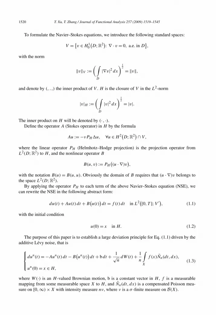
To formulate the Navier–Stokes equations, we introduce the following standard spaces:
V = {v ∈ H 1
0
(D;R
2): ∇ · v = 0, a.e. in D},
with the norm
‖v‖V :=(∫
D
|∇v|2 dx
) 12 = ‖v‖,
and denote by (, . ,) the inner product of V . H is the closure of V in the L2-norm
|v|H :=(∫
D
|v|2 dx
) 12 = |v|.
The inner product on H will be denoted by (· , ·).Define the operator A (Stokes operator) in H by the formula
Au := −νPH �u, ∀u ∈ H 2(D;R2)∩ V,
where the linear operator PH (Helmhotz–Hodge projection) is the projection operator fromL2(D;R
2) to H , and the nonlinear operator B
B(u, v) := PH
((u · ∇)v
),
with the notation B(u) = B(u,u). Obviously the domain of B requires that (u · ∇)v belongs tothe space L2(D;R
2).
By applying the operator PH to each term of the above Navier–Stokes equation (NSE), wecan rewrite the NSE in the following abstract form:
du(t) + Au(t) dt + B(u(t)
)dt = f (t) dt in L2([0, T ];V ′), (1.1)
with the initial condition
u(0) = x in H. (1.2)
The purpose of this paper is to establish a large deviation principle for Eq. (1.1) driven by theadditive Lévy noise, that is
⎧⎪⎨⎪⎩
dun(t) = −Aun(t) dt − B(un(t)
)dt + bdt + 1√
ndW(t) + 1
n
∫X
f (x)Nn(dt, dx),
un(0) = x ∈ H,
(1.3)
where W(·) is an H -valued Brownian motion, b is a constant vector in H , f is a measurablemapping from some measurable space X to H , and Nn(dt, dx) is a compensated Poisson mea-sure on [0,∞) × X with intensity measure nν, where ν is a σ -finite measure on B(X).

T. Xu, T. Zhang / Journal of Functional Analysis 257 (2009) 1519–1545 1521
There exists a great amount of literature on the stochastic Navier–Stokes equation. A goodreference for stochastic Navier–Stokes equations driven by additive noise is the book [5] andthe references therein. The existence and uniqueness of solutions for the 2-D stochastic Navier–Stokes equations with multiplicative Gaussian noise were obtained in [11,15,17]. The ergodicproperties and invariant measures of the 2-D stochastic Navier–Stokes equations were studiedin [10] and [13]. The small Gaussian noise large deviation of the 2-D stochastic Navier–Stokesequations was established in [17] and the large deviation of occupation measures was consideredin [12].
Large deviations for stochastic equations and stochastic partial differential equations havebeen investigated in many papers, see [1–4,19]. There is not much work on large deviations forstochastic evolution equations driven by Lévy noises in infinite dimensions. To the best of ourknowledge, [16] is the first paper on this topic, where the Lipschitz coefficients are considered.For this paper, in addition to the difficulties caused by the Lévy noise, much of the problem isto deal with the highly nonlinear term B(u,u). For this purpose, we need to prove a numberof exponential estimates for the energy of the solutions as well as the exponential convergenceof the approximating solutions. We mention that the large deviation principle for the solutionof the stochastic equation driven by jump processes in finite dimensions has been establishedin [8].
The organization of this paper is as follows. In Section 2, we collect some preliminary factswhich are frequently used in the sequel. In Section 3, we prove a number of exponential estimatesfor the solutions, which will play an important role in the rest of the paper. Section 4 is devotedto establish a large deviation principle.
2. Preliminaries
Identifying H with its dual H ′, we consider Eq. (1.3) in the framework of Gelfrand triple:
V ⊂ H ∼= H ′ ⊂ V ′.
In this way, we may consider A as a bounded operator from V into V ′. Moreover, we also denoteby 〈· , ·〉, the duality between V and V ′. Hence, for u = (ui) ∈ V , w = (wi) ∈ V , we have
〈Au,w〉 = ν∑i,j
∫D
∂iuj ∂iwj dx = ν((u,w)). (2.1)
Introduce a trilinear form on H × H × H by setting
b(u, v,w) =2∑
i,j
∫D
ui∂ivjwj dx, (2.2)
whenever the integral in (2.2) makes sense. In particular, if u,v,w ∈ V , then
⟨B(u, v),w
⟩= ⟨(u · ∇)v,w
⟩= 2∑i,j
∫ui∂ivjwj dx = b(u, v,w).
D
1522 T. Xu, T. Zhang / Journal of Functional Analysis 257 (2009) 1519–1545
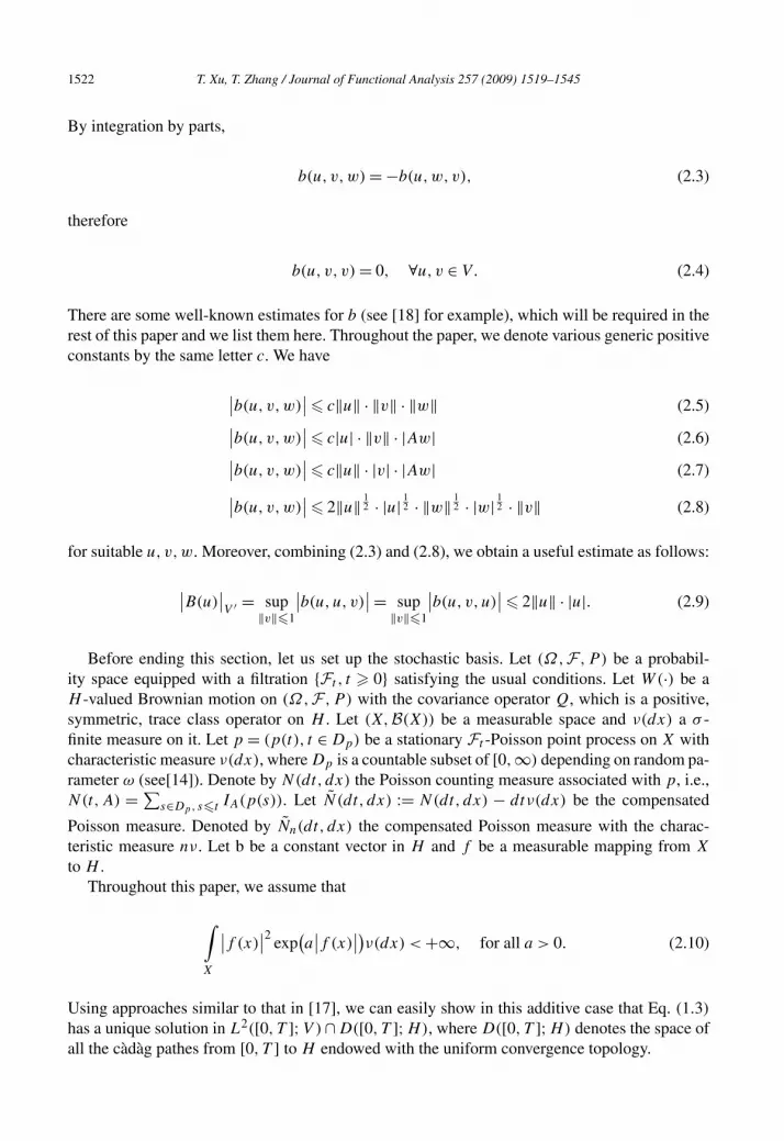
By integration by parts,
b(u, v,w) = −b(u,w,v), (2.3)
therefore
b(u, v, v) = 0, ∀u,v ∈ V. (2.4)
There are some well-known estimates for b (see [18] for example), which will be required in therest of this paper and we list them here. Throughout the paper, we denote various generic positiveconstants by the same letter c. We have
∣∣b(u, v,w)∣∣� c‖u‖ · ‖v‖ · ‖w‖ (2.5)∣∣b(u, v,w)∣∣� c|u| · ‖v‖ · |Aw| (2.6)∣∣b(u, v,w)∣∣� c‖u‖ · |v| · |Aw| (2.7)∣∣b(u, v,w)∣∣� 2‖u‖ 1
2 · |u| 12 · ‖w‖ 1
2 · |w| 12 · ‖v‖ (2.8)
for suitable u,v,w. Moreover, combining (2.3) and (2.8), we obtain a useful estimate as follows:
∣∣B(u)∣∣V ′ = sup
‖v‖�1
∣∣b(u,u, v)∣∣= sup
‖v‖�1
∣∣b(u, v,u)∣∣� 2‖u‖ · |u|. (2.9)
Before ending this section, let us set up the stochastic basis. Let (Ω, F ,P ) be a probabil-ity space equipped with a filtration {Ft , t � 0} satisfying the usual conditions. Let W(·) be aH -valued Brownian motion on (Ω, F ,P ) with the covariance operator Q, which is a positive,symmetric, trace class operator on H . Let (X, B(X)) be a measurable space and ν(dx) a σ -finite measure on it. Let p = (p(t), t ∈ Dp) be a stationary Ft -Poisson point process on X withcharacteristic measure ν(dx), where Dp is a countable subset of [0,∞) depending on random pa-rameter ω (see[14]). Denote by N(dt, dx) the Poisson counting measure associated with p, i.e.,N(t,A) = ∑
s∈Dp, s�t IA(p(s)). Let N(dt, dx) := N(dt, dx) − dtν(dx) be the compensated
Poisson measure. Denoted by Nn(dt, dx) the compensated Poisson measure with the charac-teristic measure nν. Let b be a constant vector in H and f be a measurable mapping from X
to H .Throughout this paper, we assume that
∫X
∣∣f (x)∣∣2 exp
(a∣∣f (x)
∣∣)ν(dx) < +∞, for all a > 0. (2.10)
Using approaches similar to that in [17], we can easily show in this additive case that Eq. (1.3)
has a unique solution in L2([0, T ];V ) ∩ D([0, T ];H), where D([0, T ];H) denotes the space ofall the càdàg pathes from [0, T ] to H endowed with the uniform convergence topology.

T. Xu, T. Zhang / Journal of Functional Analysis 257 (2009) 1519–1545 1523
3. Exponential estimates
To establish the large deviation principle, we first prove some exponential estimates.Let un· be the solution of the following stochastic Navier–Stokes equation
unt = x −
t∫0
Auns ds −
t∫0
B(un
s
)ds + bt + 1√
nWt + 1
n
t∫0
∫X
f (x)Nn(ds, dx). (3.1)
Let Xn· = nun· , then Xn· is the solution of the following equation
Xnt = nx −
t∫0
AXns ds − 1
n
t∫0
B(Xn
s
)ds + nbt + √
nWt +t∫
0
∫X
f (x)Nn(ds, dx). (3.2)
Denote by {ek}∞k=1 an orthonormal basis of H that consists of eigenvectors of Q in V with{λk}∞k=1 being the corresponding eigenvalues.
Lemma 3.1. For g ∈ C2b(H), Mg
t = exp(g(Xnt )−g(nx)−∫ t
0 h(Xns ) ds) is a Ft -local martingale,
where
h(y) = −⟨Ay + 1
nB(y), g′(y)
⟩+ n
(b, g′(y)
)+ n
2
∞∑k=1
λk
([g′(y) ⊗ g′(y) + g′′(y)
]ek, ek
)
+n
∫X
{exp
[g(y + f (x)
)− g(y)]− 1 − (
g′(y), f (x))}
ν(dx). (3.3)
Proof. Applying Itô’s formula to exp(g(Xnt )), we get
exp(g(Xn
t
)− g(nx))−
t∫0
exp(g(Xn
s
)− g(nx))h(Xn
s
)ds
is a local martingale. The lemma follows by another integration by parts. �In the rest of this section, we always set g(y) := (1 + λ|y|2) 1
2 (λ > 0). It is easy to see that
supy
∣∣g′′(y)∣∣� λ, sup
y
∣∣g′(y)∣∣� λ
12 .
Denote by Tr Q the trace of the operator Q, i.e., Tr Q :=∑∞i=1(Qei, ei) =∑∞
i=1 λi.
We have the following results.
Lemma 3.2. limr→∞ lim supn→∞ 1 logP(sup0�t�1 |un| > r) = −∞.
n t
1524 T. Xu, T. Zhang / Journal of Functional Analysis 257 (2009) 1519–1545
Proof. By the proof of Proposition 4.2 in [16], we know that
∣∣∣∣∫X
{exp
[g(y + f (x)
)− g(y)]− 1 − (
g′(y), f (x))}
ν(dx)
∣∣∣∣�∫X
λ∣∣f (x)
∣∣2 exp(λ
12∣∣f (x)
∣∣)ν(dx) := Mλ.
Since
⟨B(y), g′(y)
⟩= 1
2
2λ
(1 + λ|y|2) 12
⟨B(y), y
⟩= 0,
we have,
h(Xn
t
)� n|b|λ 1
2 + nλTr Q + nMλ, (3.4)
where h(·) is defined in Lemma 3.1.Observe that
P(
sup0�t�1
∣∣unt
∣∣> r)
= P(
sup0�t�1
∣∣Xnt
∣∣> nr)
= P(
sup0�t�1
g(Xn
t
)>(1 + λn2r2) 1
2)
= P
(sup
0�t�1
[g(Xn
t
)− g(nx) −t∫
0
h(Xn
s
)ds + g(nx) +
t∫0
h(Xn
s
)ds
]
>(1 + λn2r2) 1
2
)
� P
(sup
0�t�1
[g(Xn
t
)− g(nx) −t∫
0
h(Xn
s
)ds
]+ g(nx) + sup
0�t�1
t∫0
h(Xn
s
)ds
>(1 + λn2r2) 1
2
)
� P
(sup
0�t�1
[g(Xn
t
)− g(nx) −t∫
0
h(Xn
s
)ds
]
>(1 + λn2r2) 1
2 − g(nx) − sup0�t�1
t∫0
h(Xn
s
)ds
). (3.5)
Due to (3.4) and Doob’s inequality,
T. Xu, T. Zhang / Journal of Functional Analysis 257 (2009) 1519–1545 1525
P
(sup
0�t�1
(g(Xn
t
)− g(nx) −t∫
0
h(Xn
s
)ds
)>(1 + λn2r2) 1
2 − g(nx) − sup0�t�1
t∫0
h(Xn
s
)ds
)
� P
(sup
0�t�1
[g(Xn
t
)− g(nx) −t∫
0
h(Xn
s
)ds
]
>(1 + λn2r2) 1
2 − g(nx) − n|b|λ 12 − nλTr Q − nMλ
)
�(
sup0�t�1
E
[exp
(g(Xn
t
)− g(nx) −t∫
0
h(Xn
s
)ds
)])
× exp[−(
1 + λn2r2) 12 + g(nx) + n|b|λ 1
2 + nλTr Q + nMλ
]� exp
[−(1 + λn2r2) 1
2 + g(nx) + n|b|λ 12 + nλTr Q + nMλ
], (3.6)
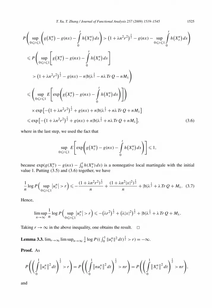
where in the last step, we used the fact that
sup0�t�1
E
[exp
(g(Xn
t
)− g(nx) −t∫
0
h(Xn
s
)ds
)]� 1,
because exp(g(Xnt ) − g(nx) − ∫ t
0 h(Xns ) ds) is a nonnegative local martingale with the initial
value 1. Putting (3.5) and (3.6) together, we have
1
nlogP
(sup
0�t�1
∣∣unt
∣∣> r)
� − (1 + λn2r2)12
n+ (1 + λn2|x|2) 1
2
n+ |b|λ 1
2 + λTr Q + Mλ. (3.7)
Hence,
lim supn→∞
1
nlogP
(sup
0�t�1
∣∣unt
∣∣> r)
� −(λr2) 1
2 + (λ|x|2) 1
2 + |b|λ 12 + λTr Q + Mλ.
Taking r → ∞ in the above inequality, one obtains the result. �Lemma 3.3. limr→∞ lim supn→∞ 1
nlogP((
∫ 10 ‖un
t ‖2 dt)12 > r) = −∞.
Proof. As
P
(( 1∫0
∥∥unt
∥∥2dt
) 12
> r
)= P
(( 1∫0
∥∥nunt
∥∥2dt
) 12
> nr
)= P
(( 1∫0
∥∥Xnt
∥∥2dt
) 12
> nr
),
and
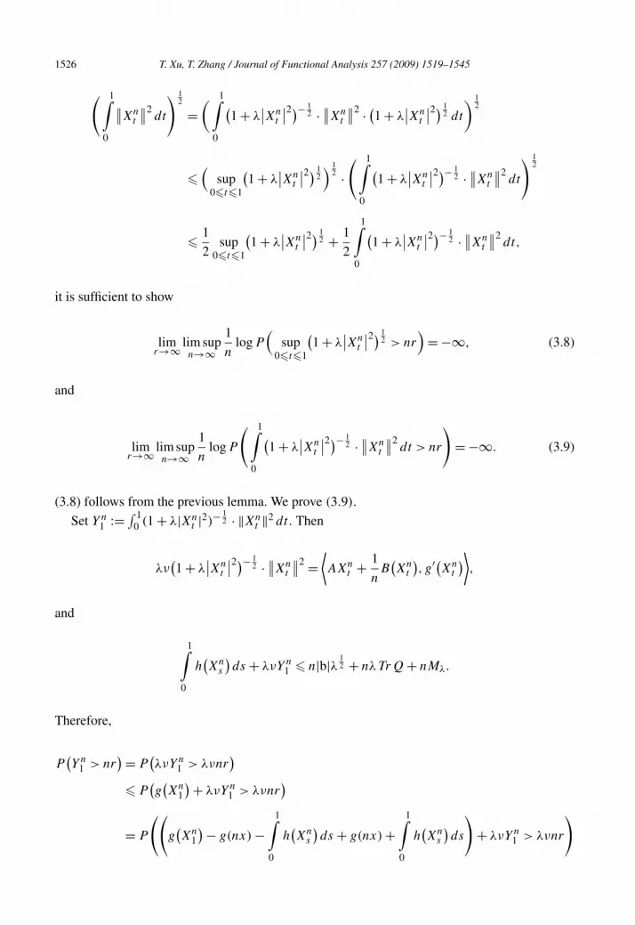
1526 T. Xu, T. Zhang / Journal of Functional Analysis 257 (2009) 1519–1545
( 1∫0
∥∥Xnt
∥∥2dt
) 12
=( 1∫
0
(1 + λ
∣∣Xnt
∣∣2)− 12 · ∥∥Xn
t
∥∥2 · (1 + λ∣∣Xn
t
∣∣2) 12 dt
) 12
�(
sup0�t�1
(1 + λ
∣∣Xnt
∣∣2) 12) 1
2 ·( 1∫
0
(1 + λ
∣∣Xnt
∣∣2)− 12 · ∥∥Xn
t
∥∥2dt
) 12
� 1
2sup
0�t�1
(1 + λ
∣∣Xnt
∣∣2) 12 + 1
2
1∫0
(1 + λ
∣∣Xnt
∣∣2)− 12 · ∥∥Xn
t
∥∥2dt,
it is sufficient to show
limr→∞ lim sup
n→∞1
nlogP
(sup
0�t�1
(1 + λ
∣∣Xnt
∣∣2) 12 > nr
)= −∞, (3.8)
and
limr→∞ lim sup
n→∞1
nlogP
( 1∫0
(1 + λ
∣∣Xnt
∣∣2)− 12 · ∥∥Xn
t
∥∥2dt > nr
)= −∞. (3.9)
(3.8) follows from the previous lemma. We prove (3.9).
Set Yn1 := ∫ 1
0 (1 + λ|Xnt |2)− 1
2 · ‖Xnt ‖2 dt. Then
λν(1 + λ
∣∣Xnt
∣∣2)− 12 · ∥∥Xn
t
∥∥2 =⟨AXn
t + 1
nB(Xn
t
), g′(Xn
t
)⟩,
and
1∫0
h(Xn
s
)ds + λνYn
1 � n|b|λ 12 + nλTr Q + nMλ.
Therefore,
P(Yn
1 > nr)= P
(λνYn
1 > λνnr)
� P(g(Xn
1
)+ λνYn1 > λνnr
)
= P
((g(Xn
1
)− g(nx) −1∫h(Xn
s
)ds + g(nx) +
1∫h(Xn
s
)ds
)+ λνYn
1 > λνnr
)
0 0
T. Xu, T. Zhang / Journal of Functional Analysis 257 (2009) 1519–1545 1527
� P
((g(Xn
1
)− g(nx) −1∫
0
h(Xn
s
)ds
)> λνnr − (
1 + λn2|x|2) 12
− n
(|b|λ 1
2 + λTr Q + Mλ
))
� exp
(−λνnr + (
1 + λn2|x|2) 12 + n
(|b|λ 1
2 + λTr Q + Mλ
)), (3.10)
which yields
limr→∞ lim sup
n→∞1
nlogP
(Yn
1 > nr)= −∞,
completing the proof. �Define the projection operator Pm by
Pmx :=m∑
i=1
(x, ei)ei, x ∈ H.
Let Zn,mt ,Zn
t be the solutions of the following linear equations respectively,
Zn,mt = −
t∫0
AZn,ms ds + 1
n
t∫0
∫X
Pmf (x)Nn(ds, dx), (3.11)
and
Znt = −
t∫0
AZns ds + 1
n
t∫0
∫X
f (x)Nn(ds, dx). (3.12)
Put Zn,mt := n(Z
n,mt − Zn
t ), then Zn,mt is the solution of the equation
Zn,mt = −
t∫0
AZn,ms ds +
t∫0
∫X
(Pmf (x) − f (x)
)Nn(ds, dx). (3.13)
Similar to the proof of Lemma 3.1, one has
exp
(g(Z
n,mt
)− g(0) −t∫
0
h(Zn,m
s
)ds
)is a Ft -local martingale, (3.14)
where

1528 T. Xu, T. Zhang / Journal of Functional Analysis 257 (2009) 1519–1545
h(y) = −⟨Ay,g′(y)
⟩+ n
∫X
{exp
[g(y + Pmf (x) − f (x)
)− g(y)]− 1
− (g′(y),Pmf (x) − f (x)
)}ν(dx).
Lemma 3.4. For any δ > 0,
limm→∞ lim sup
n→∞1
nlogP
( 1∫0
∥∥Zn,ms − Zn
s
∥∥2ds > δ
)= −∞.
Proof. By Lemma 5.6 in [16], we know that, for any δ > 0,
limm→∞ lim sup
n→∞1
nlogP
(sup
0�t�1
∣∣Zn,mt − Zn
t
∣∣> δ)
= −∞. (3.15)
Define a stopping time by
τn,m1 := inf
{t � 0,
∣∣Zn,mt − Zn
t
∣∣> 1},
then
P
( 1∫0
∥∥Zn,ms − Zn
s
∥∥2ds > δ, sup
0�t�1
∣∣Zn,mt − Zn
t
∣∣� 1
)
� P
( 1∫0
∥∥Zn,ms − Zn
s
∥∥2ds > δ,1 � τ
n,m1
)
� P
( 1∧τn,m1∫
0
∥∥Zn,ms − Zn
s
∥∥2ds > δ
)
� P
(sup
0�t�1∧τn,m1
(g(nZ
n,mt− − nZn
t−))
×1∧τ
n,m1∫
0
g−1(nZn,ms − nZn
s
) · ∥∥nZn,ms − nZn
s
∥∥2ds > n2δ
),
where in the last step, we have used the fact that {s: nZn,ms− −nZn
s− �= nZn,ms −nZn
s } is countable.By the definition of g and the stopping time τ
n,m, we get
1
T. Xu, T. Zhang / Journal of Functional Analysis 257 (2009) 1519–1545 1529
P
(sup
0�t�1∧τn,m1
(g(nZ
n,mt− − nZn
t−)) ·
1∧τn,m1∫
0
g−1(nZn,ms − nZn
s
) · ∥∥nZn,ms − nZn
s
∥∥2ds > n2δ
)
� P
( 1∧τn,m1∫
0
g−1(nZn,ms − nZn
s
) · ∥∥nZn,ms − nZn
s
∥∥2ds >
n2δ
(1 + λn2)12
).
Set Zn,mt := ∫ t
0 g−1(Zn,ms ) · ‖Zn,m
s ‖2 ds, then
1∧τn,m1∫
0
h(Z
n,mt
)+ λνZn,m
1∧τn,m1
� nMλ,m, (3.16)
where
Mλ,m = λ
∫X
exp
(λ
12∣∣Pmf (x) − f (x)
∣∣) · (∣∣Pmf (x) − f (x)∣∣2)ν(dx).
As in the proof of (3.10), we have
P
(Z
n,m
1∧τn,m1
>n2δ
(1 + λn2)12
)
= P
(λνZ
n,m
1∧τn,m1
>λνn2δ
(1 + λn2)12
)
� P
(g(Z
n,m
1∧τn,m1
)+ λνZn,m
1∧τn,m1
>λνn2δ
(1 + λn2)12
)
� P
([g(Z
n,m
1∧τn,m1
)− g(0) −1∧τ
n,m1∫
0
h(Zn,m
s
)ds + g(0) +
1∧τn,m1∫
0
h(Zn,m
s
)ds
]+ λνZ
n,m
1∧τn,m1
>λνn2δ
(1 + λn2)12
)
� P
(g(Z
n,m
1∧τn,m1
)− g(0) −1∧τ
n,m1∫
0
h(Zn,m
s
)ds
)>
λνn2δ
(1 + λn2)12
− g(0) − nMλ,m)
� exp
(− λνn2δ
(1 + λn2)12
+ 1 + nMλ,m
),
where we used the fact in (3.14). Therefore,

1530 T. Xu, T. Zhang / Journal of Functional Analysis 257 (2009) 1519–1545
lim supn→∞
1
nlogP
( 1∫0
∥∥Zn,ms − Zn
s
∥∥2ds > δ, sup
0�t�1
∣∣Zn,mt − Zn
t
∣∣� 1
)� −νδλ
12 + Mλ,m. (3.17)
Since limm→∞ Mλ,m = 0, let m → ∞ in (3.17) to obtain
limm→∞ lim sup
n→∞1
nlogP
( 1∫0
∥∥Zn,ms − Zn
s
∥∥2ds > δ, sup
0�t�1
∣∣Zn,mt − Zn
t
∣∣� 1
)� −νδλ
12 .
Since λ is arbitrary, taking λ → ∞ in the above inequality, we obtain
limm→∞ lim sup
n→∞1
nlogP
( 1∫0
∥∥Zn,ms − Zn
s
∥∥2ds > δ, sup
0�t�1
∣∣Zn,mt − Zn
t
∣∣� 1
)= −∞.
Combining with (3.15) proves the lemma. �4. Large deviation principle
First, we state the main result of this paper. For l ∈ H , define
F(l) :=∫X
[exp
(f (x), l
)− 1 − (f (x), l
)]ν(dx) + (Ql, l) + (b, l).
Set, for z ∈ H,
F ∗(z) = supl∈H
[(z, l) − F(l)
].
Let
Lnt := bt + 1√
nWt + 1
n
t∫0
∫X
f (x)Nn(ds, dx),
then by [7], we know that the laws of {Ln· , n � 1} satisfy a large deviation principle onD([0,1];H) with the rate function I0, which is defined by
I0(g) : ={∫ 1
0 F ∗(g′(s)) ds, if g ∈ D([0,1];H), g′ ∈ L1([0,1];H),
∞, otherwise.
For g ∈ D([0,1];H) with g′ ∈ L1([0,1];H), define φ(g) ∈ D([0,1];H) ∩ L2([0,1];V ) to bethe solution of the following equation
φt (g) = x −t∫Aφs(g)ds −
t∫B(φs(g)
)ds + g(t). (4.1)
0 0

T. Xu, T. Zhang / Journal of Functional Analysis 257 (2009) 1519–1545 1531
Set, for h ∈ D([0,1];H),
I (h) := inf{I0(g): h = φ(g), g ∈ D
([0,1];H )}with the convention inf{∅} = ∞.
Theorem 4.1. Let μn be the law of the solution un of Eq. (1.3), then {μn,n � 1} satisfies a largedeviation principle on D([0,1];H) endowed with the uniform topology with the rate functionI (·), i.e.,
(i) For any closed subset F ⊂ D([0,1];H),
lim supn→∞
1
nlogμn(F ) � − inf
h∈FI (h).
(ii) For any open set G ⊂ D([0,1];H),
lim infn→∞
1
nlogμn(G) � − inf
h∈GI (h).
According to the generalized contraction principle in the theory of large deviations (see The-orem 4.1 in [9]), Theorem 4.1 will follow from the following Lemmas 4.1–4.3.
Lemma 4.1. The mapping φ defined in (4.1) is continuous from D([0,1];V ) into D([0,1];H)∩L2([0,1];V ) in the topology of uniform convergence.
Proof. Let vt (g) = φt (g) − g(t), then vt (g) satisfies the following equation
vt (g) = x −t∫
0
Avs(g) ds −t∫
0
Ag(s) ds −t∫
0
B(vs(g) + g(s)
)ds.
It is sufficient to show that
v(·) : D([0,1];V )→ D([0,1];H )∩ L2([0,1];V )
is continuous,
that is, take {gn}∞n=1, g ∈ D([0,1];V ) such that limn→∞ sup0�t�1 ‖gn(t) − g(t)‖ = 0, then
limn→∞
(sup
0�t�1
∣∣vt (g) − vt (gn)∣∣2 + ν
2
1∫0
∥∥vs(g) − vs(gn)∥∥2
ds
)= 0.
To this end, we need some energy estimates for vt (g). In view of (2.3), (2.4), (2.5), and (2.9),we have
1532 T. Xu, T. Zhang / Journal of Functional Analysis 257 (2009) 1519–1545
∣∣vt (g)∣∣2 + 2ν
t∫0
∥∥vs(g)∥∥2
ds
= |x|2 − 2
t∫0
⟨Ag(s), vs(g)
⟩ds − 2
t∫0
⟨B(vs(g) + g(s)
), vs(g)
⟩ds
� |x|2 + ν
t∫0
∥∥vs(g)∥∥2
ds + 1
ν
t∫0
∥∥g(s)∥∥2
ds + 2
t∫0
∣∣⟨B(vs(g) + g(s)), vs(g)
⟩∣∣ds
� |x|2 + ν
t∫0
∥∥vs(g)∥∥2
ds + 1
ν
t∫0
∥∥g(s)∥∥2
ds + 2
t∫0
∣∣b(vs(g), g(s), vs(g))∣∣ds
+ 2
t∫0
∣∣b(g(s), g(s), vs(g))∣∣ds
� |x|2 + ν
t∫0
∥∥vs(g)∥∥2
ds + 1
ν
t∫0
∥∥g(s)∥∥2
ds + 4
t∫0
∣∣vs(g)∣∣ · ∥∥g(s)
∥∥ · ∥∥vs(g)∥∥ds
+ 4c
t∫0
∥∥g(s)∥∥2∥∥vs(g)
∥∥ds
� |x|2 + 3ν
2
t∫0
∥∥vs(g)∥∥2
ds + 1
ν
t∫0
∥∥g(s)∥∥2
ds + 16
ν
t∫0
∣∣vs(g)∣∣2∥∥g(s)
∥∥2ds
+ 16c2
ν
t∫0
∥∥g(s)∥∥4
ds. (4.2)
Applying Gronwall’s inequality, we have
sup0�s�t
∣∣vs(g)∣∣2 �
(|x|2 + 1
ν
t∫0
∥∥g(s)∥∥2
ds + 16c2
ν
t∫0
∥∥g(s)∥∥4
ds
)exp
(16
ν
t∫0
∥∥g(s)∥∥2
ds
)
�[|x|2 + t
(1
νsup
0�s�t
∥∥g(s)∥∥2 + 16c2
νsup
0�s�t
∥∥g(s)∥∥4)]
exp
(16
νt sup
0�s�t
∥∥g(s)∥∥2)
.
(4.3)
Furthermore,

T. Xu, T. Zhang / Journal of Functional Analysis 257 (2009) 1519–1545 1533
ν
2
t∫0
∥∥vs(g)∥∥2
ds
� |x|2 + 1
νt(
sup0�s�t
∥∥g(s)∥∥2 + 16 sup
0�s�t
∥∥g(s)∥∥2
Mt(g) + 16c2 sup0�s�t
∥∥g(s)∥∥4), (4.4)
where
Mg(t) =[|x|2 + t
(1
νsup
0�s�t
∥∥g(s)∥∥2 + 16c2
νsup
0�s�t
∥∥g(s)∥∥4)]
exp
(16
νt sup
0�s�t
∥∥g(s)∥∥2)
.
It is easy to see that, if g is replaced by gn, (4.3), (4.4) still hold. Since
limn→∞ sup
0�t�1
∥∥gn(t) − g(t)∥∥2 = 0,
there exists a constant Cg(x) depending on sup0�t�1 ‖g(t)‖ and |x|2 (which may change line toline) such that
1∫0
∥∥vs(gn)∥∥2
ds � Cg(x) (n � 1). (4.5)
Now by the chain rule, one has
∣∣vt (gn) − vt (g)∣∣2 + 2ν
t∫0
∥∥vs(gn) − vs(g)∥∥2
ds
= −2
t∫0
⟨Agn(s) − Ag(s), vs(gn) − vs(g)
⟩ds
− 2
t∫0
⟨B(vs(gn) + gn(s)
)− B(vs(g) + g(s)
), vs(gn) − vs(g)
⟩ds
� ν
t∫0
∥∥vs(gn) − vs(g)∥∥2
ds + 1
ν
t∫0
∥∥gn(s) − g(s)∥∥2
ds
+ 2
t∫0
∣∣⟨B(vs(gn) + gn(s))− B
(vs(g) + g(s)
), vs(gn) − vs(g)
⟩∣∣ds. (4.6)

1534 T. Xu, T. Zhang / Journal of Functional Analysis 257 (2009) 1519–1545
Now, due to (2.3), (2.4), (2.5) and (2.9),
∣∣⟨B(vs(gn) + gn(s))− B
(vs(g) + g(s)
), vs(gn) − vs(g)
⟩∣∣�∣∣b(vs(gn) + gn(s), vs(gn) + gn(s), vs(gn) − vs(g)
)− b
(vs(g) + g(s), vs(gn) + gn(s), vs(gn) − vs(g)
)∣∣+ ∣∣b(vs(g) + g(s), vs(g) + g(s), vs(gn) − vs(g)
)− b
(vs(g) + g(s), vs(gn) + gn(s), vs(gn) − vs(g)
)∣∣�∣∣b(vs(gn) − vs(g), vs(gn) + gn(s), vs(gn) − vs(g)
)∣∣+ ∣∣b(gn(s) − g(s), vs(gn) + gn(s), vs(gn) − vs(g)
)∣∣+ ∣∣b(vs(g) + g(s), gn(s) − g(s), vs(gn) − vs(g)
)∣∣� 2
∣∣vs(gn) − vs(g)∣∣ · ∥∥vs(gn) − vs(g)
∥∥ · ∥∥vs(gn) + gn(s)∥∥
+ 2c∥∥gn(s) − g(s)
∥∥ · ∥∥vs(gn) + gn(s)∥∥ · ∥∥vs(gn) − vs(g)
∥∥+ 2c
∥∥vs(g) + g(s)| · ∥∥gn(s) − g(s)
∥∥ · ∥∥vs(gn) − vs(g)∥∥
� ν
12
∥∥vs(gn) − vs(g)∥∥2 + 12
ν
(∥∥vs(g)∥∥+ ∥∥gn(s)
∥∥)2 · ∣∣vs(gn) − vs(g)∣∣2
+ ν
12
∥∥vs(gn) − vs(g)∥∥2 + 12c2
ν
(∥∥vs(gn)∥∥+ ∥∥gn(s)
∥∥)2 · ∥∥gn(s) − g(s)∥∥2
+ ν
12
∥∥vs(gn) − vs(g)∥∥2 + 12c2
ν
(∥∥vs(g)∥∥+ ∥∥g(s)
∥∥)2 · ∥∥gn(s) − g(s)∥∥2
. (4.7)
Combining (4.6) and (4.7), one obtains
∣∣vt (gn) − vt (g)∣∣2 + ν
2
t∫0
∥∥vs(gn) − vs(g)∥∥2
ds
� 1
ν
t∫0
∥∥gn(s) − g(s)∥∥2
ds + 24
ν
t∫0
(∥∥vs(g)∥∥+ ∥∥gn(s)
∥∥)2 · ∣∣vs(gn) − vs(g)∣∣2 ds
+ 24c2
ν
t∫0
(∥∥vs(gn)∥∥+ ∥∥gn(s)
∥∥)2 · ∥∥gn(s) − g(s)∥∥2
ds
+ 24c2
ν
t∫0
(∥∥vs(g)∥∥+ ∥∥g(s)
∥∥)2 · ∥∥gn(s) − g(s)∥∥2
ds.
Applying Gronwall’s inequality and (4.5), we arrive at

T. Xu, T. Zhang / Journal of Functional Analysis 257 (2009) 1519–1545 1535
sup0�t�1
∣∣vt (gn) − vt (g)∣∣2 + ν
2
1∫0
∥∥vs(gn) − vs(g)∥∥2
ds
�(
48c2
ν
1∫0
[(∥∥vs(gn)∥∥+ ∥∥gn(s)
∥∥)2 + (∥∥vs(g)∥∥+ ∥∥g(s)
∥∥)2] · ∥∥gn(s) − g(s)∥∥2
ds
+ 2
ν
1∫0
∥∥gn(s) − g(s)∥∥2
ds
)× exp
(48
ν
1∫0
(∥∥vs(gn)∥∥+ ∥∥gn(s)
∥∥)2ds
)
�(
2
ν+ 48c2
ν
)Cg(x) sup
0�t�1
∥∥gn(t) − g(t)∥∥2
.
Let n → ∞ to prove the lemma. �Now, let un,m· be the solution of the equation
un,mt = x −
t∫0
Aun,ms ds −
t∫0
B(un,m
s
)ds + bmt + 1√
nWm
t + 1
n
t∫0
∫X
f m(x)Nn(ds, dx), (4.8)
where bm = Pmb, Wmt = PmWt , f m(x) = Pmf (x). Recall that Zn,m,Zn are defined as in (3.11)
and (3.12). Set un,mt := u
n,mt − Z
n,mt , un
t := unt − Zn
t . Then un,mt and un
t satisfy
un,mt = x −
t∫0
Aun,ms ds −
t∫0
B(un,m
s + Zn,ms
)ds + bmt + 1√
nWm
t ,
and
unt = x −
t∫0
Auns ds −
t∫0
B(un
s + Zns
)ds + bt + 1√
nWt .
Lemma 4.2. For any δ > 0,
limm→∞ lim sup
n→∞1
nlogP
(sup
0�t�1
∣∣un,mt − un
t
∣∣> δ)
= −∞.
Proof. Note that
P(
sup0�t�1
∣∣un,mt − un
t
∣∣> δ)
� P
(sup
∣∣un,mt − un
t
∣∣> δ
2
)+ P
(sup
∣∣Zn,mt − Zn
t
∣∣> δ
2
). (4.9)
0�t�1 0�t�1

1536 T. Xu, T. Zhang / Journal of Functional Analysis 257 (2009) 1519–1545
By Lemma 5.6 in [16], we know that
limm→∞ lim sup
n→∞1
nlogP
(sup
0�t�1
∣∣Zn,mt − Zn
t
∣∣> δ
2
)= −∞. (4.10)
It suffices to prove, for any δ > 0,
limm→∞ lim sup
n→∞1
nlogP
(sup
0�t�1
∣∣un,mt − un
t
∣∣> δ
2
)= −∞. (4.11)
For δ0 > 0, define a stopping time by
τn,mδ0
:= inf
{t � 0,
∣∣Zn,mt − Zn
t
∣∣> δ0 or
t∫0
∥∥Zn,ms − Zn
s
∥∥2ds > δ0
}.
Note that Lemma 3.2 and Lemma 3.3 still hold for un,m· , Zn,m· and Zn· , when m is fixed. Definestopping times τn
u,1,M , τnu,2,M by
τnu,1,M := inf
{t � 0,
∣∣un(t)∣∣> M
},
and
τnu,2,M := inf
{t � 0,
t∫0
∥∥uns
∥∥2ds > M
}.
We can also define similar stopping times for un,m· , Zn,m· and Zn· . We denote these stopping timesby τ
n,mu,1,M , τ
n,mu,2,M , τn
Z,1,M , τnZ,2,M , τ
n,mZ,1,M and τ
n,mZ,2,M , respectively. Let
τn,mM := τn
u,1,M ∧ τnu,2,M ∧ τ
n,mu,1,M ∧ τ
n,mu,2,M ∧ τn
Z,1,M ∧ τnZ,2,M ∧ τ
n,mZ,1,M ∧ τ
n,mZ,2,M,
and set
An,m(ω) :={
sup0�t�1
∣∣un,mt
∣∣� M}
∩{
sup0�t�1
∣∣unt
∣∣� M}
∩{
sup0�t�1
∣∣Zn,mt
∣∣� M}
∩{
sup0�t�1
∣∣Znt
∣∣� M},
Bn,m(ω) : ={ 1∫
0
∥∥un,ms
∥∥2ds � M
}∩{ 1∫
0
∥∥uns
∥∥2ds � M
}∩{ 1∫
0
∥∥Zn,ms
∥∥2ds � M
}
∩{ 1∫ ∥∥Zn
s
∥∥2ds � M
},
0

T. Xu, T. Zhang / Journal of Functional Analysis 257 (2009) 1519–1545 1537
Cn,m(ω) :={
sup0�t�1
∣∣Zn,mt − Zn
t
∣∣� δ0,
1∫0
∥∥Zn,mt − Zn
t
∥∥2dt � δ0
}.
Then,
P({
sup0�t�1
∣∣un,mt − un
t
∣∣> δ}
∩ An,m ∩ Bn,m ∩ Cn,m)
� P(
sup0�t�1
∣∣un,mt − un
t
∣∣> δ,1 � τn,mM ∧ τ
n,mδ0
)
� P(
sup0�t�1∧τ
n,mM ∧τ
n,mδ0
∣∣un,mt − un
t
∣∣> δ)
= P(
sup0�t�1∧τ
n,mM ∧τ
n,mδ0
∣∣un,mt − un
t
∣∣2 > δ2). (4.12)
Applying Itô’s formula to |un,m
t∧τn,mM ∧τ
n,mδ0
− unt∧τ
n,mM ∧τ
n,mδ0
|2, we have
∣∣un,m
t∧τn,mM ∧τ
n,mδ0
− unt∧τ
n,mM ∧τ
n,mδ0
∣∣2 + 2ν
t∧τn,mM ∧τ
n,mδ0∫
0
∥∥un,ms − un
s
∥∥2ds
= −2
t∧τn,mM ∧τ
n,mδ0∫
0
⟨B(un,m
s + Zn,ms
)− B(un
s + Zns
), un,m
s − uns
⟩ds
+ 2
t∧τn,mM ∧τ
n,mδ0∫
0
(un,m
s − uns ,bm − b
)ds + 1
n
t∧τn,mM ∧τ
n,mδ0∫
0
∞∑i=m+1
λids
+ 2√n
t∧τn,mM ∧τ
n,mδ0∫
0
(un,m
s − uns , dWm
s − dWs
), (4.13)
thus,
sup0�s�t∧τ
n,mM ∧τ
n,mδ0
∣∣un,ms − un
s
∣∣2 + 2ν
t∧τn,mm ∧τ
n,mδ0∫
0
∥∥un,ms − un
s
∥∥2ds
� 4
t∧τn,mM ∧τ
n,mδ0∫ ∣∣⟨B(un,m
s + Zn,ms
)− B(un
s + Zns
), un,m
s − uns
⟩∣∣ds
0

1538 T. Xu, T. Zhang / Journal of Functional Analysis 257 (2009) 1519–1545
+ 4
t∧τn,mM ∧τ
n,mδ0∫
0
∣∣(un,ms − un
s , bm − b
)∣∣ds + 2
n
t∫0
∞∑i=m+1
λi ds
+ 4√n
sup0�s�t∧τ
n,mM ∧τ
n,mδ0
∣∣∣∣∣s∫
0
(un,m
r − unr , dWm
r − dWr
)∣∣∣∣∣. (4.14)
Write,
t∫0
⟨B(un,m
s + Zn,ms
)− B(un
s + Zns
), un,m
s − uns
⟩ds
=t∫
0
b(un,m
s + Zn,ms , un,m
s + Zn,ms , un,m
s − uns
)− b(un
s + Zns , un
s + Zns , un,m
s − uns
)ds
=t∫
0
b(un,m
s , un,ms , un,m
s − uns
)− b(un
s , uns , u
n,ms − un
s
)ds
+t∫
0
b(un,m
s ,Zn,ms , un,m
s − uns
)− b(un
s ,Zns , un,m
s − uns
)ds
+t∫
0
b(Zn,m
s , un,ms , un,m
s − uns
)− b(Zn
s , uns , u
n,ms − un
s
)ds
+t∫
0
b(Zn,m
s ,Zn,ms , un,m
s − uns
)− b(Zn
s ,Zns , un,m
s − uns
)ds
=: II1 + II2 + II3 + II4. (4.15)
By virtue of the properties of b(· , · , ·), we have,
|II1| � 2
t∫0
∣∣un,ms − un
s
∣∣ · ∥∥uns
∥∥ · ∥∥un,ms − un
s
∥∥ds
� ν
24
t∫0
∥∥un,ms − un
s
∥∥2ds + 24
ν
t∫0
∣∣un,ms − un
s
∣∣2 · ∥∥uns
∥∥2ds, (4.16)
|II2| �t∫ ∣∣b(un,m
s − uns ,Z
n,ms , un,m
s − uns
)∣∣ds +t∫ ∣∣b(un
s ,Zn,ms − Zn
s , un,ms − un
s
)∣∣ds
0 0

T. Xu, T. Zhang / Journal of Functional Analysis 257 (2009) 1519–1545 1539
� 2
t∫0
∣∣un,ms − un
s
∣∣ · ∥∥Zn,ms
∥∥ · ∥∥un,ms − un
s
∥∥ds
+ 2
t∫0
∣∣uns
∣∣ 12 · ∥∥un
s
∥∥ 12 · ∣∣Zn,m
s − Zns
∣∣ 12 · ∥∥Zn,m
s − Zns
∥∥ 12 · ∥∥un,m
s − uns
∥∥ds
� ν
24
t∫0
∥∥un,ms − un
s
∥∥2ds + 24
ν
t∫0
∣∣un,ms − un
s
∣∣2 · ∥∥Zn,ms
∥∥2ds + ν
24
t∫0
∥∥un,ms − un
s
∥∥2ds
+ 24
νsup
0�s�t
∣∣Zn,ms− − Zn
s−∣∣ · sup
0�s�t
∣∣uns−∣∣ ·( t∫
0
∥∥Zn,ms − Zn
s
∥∥2ds
) 12
·( t∫
0
∥∥uns
∥∥2ds
) 12
,
(4.17)
|II3| � 2
t∫0
∣∣Zn,ms − Zn
s
∣∣ 12 · ∥∥Zn,m
s − Zns
∥∥ 12 · ∣∣un
s
∣∣ 12 · ∥∥un
s
∥∥ 12 · ∥∥un,m
s − uns
∥∥ds
� ν
24
t∫0
∥∥un,ms − un
s
∥∥2ds + 24
νsup
0�s�t
∣∣Zn,ms− − Zn
s−∣∣ · sup
0�s�t
∣∣uns−∣∣( t∫
0
∥∥Zn,ms − Zn
s
∥∥2ds
) 12
×( t∫
0
∥∥uns
∥∥2ds
) 12
, (4.18)
and similarly
|II4| �t∫
0
∣∣b(Zn,ms − Zn
s ,Zn,ms , un,m
s − uns
)∣∣ds +t∫
0
∣∣b(Zns ,Zn,m
s − Zns , un,m
s − uns
)∣∣ds
� ν
24
t∫0
∥∥un,ms − un
s
∥∥2ds + 24
νsup
0�s�t
∣∣Zn,ms− − Zn
s−∣∣ · sup
0�s�t
∣∣Zn,ms−
∣∣( t∫0
∥∥Zn,ms − Zn
s
∥∥2ds
) 12
×( t∫
0
∥∥Zn,ms
∥∥2ds
) 12
+ ν
24
t∫0
∥∥un,ms − un
s
∥∥2ds + 24
νsup
0�s�t
∣∣Zn,ms− − Zn
s−∣∣
× sup0�s�t
∣∣Zns−∣∣( t∫ ∥∥Zn,m
s − Zns
∥∥2ds
) 12
·( t∫ ∥∥Zn
s
∥∥2ds
) 12
. (4.19)
0 0
1540 T. Xu, T. Zhang / Journal of Functional Analysis 257 (2009) 1519–1545
Note that we have used the fact that {s: Zns �= Zn
s−} is countable P-a.s. This fact is also true forZn,m· and Zn,m· − Zn· .
Set Mt := 4√n
∫ t
0 (un,ms − un
s , dWms −dWs), and putting (4.16)–(4.19) and (4.14) together, one
obtains
1
2sup
0�s�t∧τn,mM ∧τ
n,mδ0
∣∣un,ms − un
s
∣∣2 + ν
t∧τn,mM ∧τ
n,mδ0∫
0
∥∥un,ms − un
s
∥∥2ds
�(
2t
n
∞∑i=m+1
λi + sup0�s�t∧τ
n,mM ∧τ
n,mδ0
|Mt | + 8|bm − b|2t2 + c
ν(δ0M)
32
)
+ c
ν
t∧τn,mM ∧τ
n,mδ0∫
0
∣∣un,ms − un
s
∣∣2 · (∥∥uns
∥∥2 + ∥∥Zn,ms
∥∥2)ds. (4.20)
Note that c is a constant independent of n,m. Applying Gronwall’s inequality, we get
sup0�s�t∧τ
n,mM ∧τ
n,mδ0
∣∣un,ms − un
s
∣∣2
�(
4t
n
∞∑i=m+1
λi + 2 sup0�s�t∧τ
n,mM ∧τ
n,mδ0
|Mt | + 16|bm − b|2t2 + c
ν(δ0M)
32
)
× expcν
∫ t∧τn,mM
∧τn,mδ0
0 (‖uns ‖2+‖Zn,m
s ‖2) ds
�(
4t
n
∞∑i=m+1
λi + 2 sup0�s�t∧τ
n,mM ∧τ
n,mδ0
|Mt | + 16|bm − b|2t2 + c
ν(δ0M)
32
)
× exp
(2Mc
ν
). (4.21)
Set CM := exp ( 2Mcν
). Applying the martingale inequality in [6] to M·, it follows that
[E(
sup0�s�t∧τ
n,mM ∧τ
n,mδ0
∣∣un,ms − un
s
∣∣2p)] 2
p
� 2
(4t
n
∞∑i=m+1
λi + 16|bm − b|2t2 + c
ν(δ0M)
32
)2
C2M
+ 8(E sup
0�s�t∧τn,m∧τ
n,m|Mt |p
) 2p C2
M
M δ0

T. Xu, T. Zhang / Journal of Functional Analysis 257 (2009) 1519–1545 1541
� 2
(4t
n
∞∑i=m+1
λi + 16|bm − b|2t2 + c
ν(δ0M)
32
)2
C2M
+ cC2M
np
[E
( t∧τn,mM ∧τ
n,mδ0∫
0
∞∑i=m+1
λ2i
∣∣un,ms − un
s
∣∣2 ds
) p2] 2
p
� 2
(4t
n
∞∑i=m+1
λi + 16|bm − b|2t2 + c
ν(δ0M)
32
)2
C2M + cC2
M
np
( ∞∑i=m+1
λ2i
)2
t
+ cC2M
np
t∫0
[E(∣∣un,m
s∧τn,mM ∧τ
n,mδ0
− uns∧τ
n,mM ∧τ
n,mδ0
∣∣)2p] 2p ds. (4.22)
Applying Gronwall’s inequality to (4.22), one obtains
[E(
sup0�s�1∧τ
n,mM ∧τ
n,mδ0
∣∣un,ms − un
s
∣∣2p)] 2
p
�[
2
(4
n
∞∑i=m+1
λi + 16|bm − b|2 + c
ν(δ0M)
32
)2
C2M + cC2
M
np
( ∞∑i=m+1
λ2i
)2]
× exp
(cC2
M
np
). (4.23)
Take p = 2n to obtain
limm→∞ lim sup
n→∞1
nlogP
(sup
0�s�1∧τn,mM ∧τ
n,mδ0
∣∣un,ms − un
s
∣∣2 > δ2)
� limm→∞ lim sup
n→∞log
[E(
sup0�s�1∧τ
n,mM ∧τ
n,mδ0
∣∣un,ms − un
s
∣∣2p)] 2
p − log δ4
� 2 log
(√2c
ν(δ0M)
32 CM
)+ 2cC2
M − 4 log δ. (4.24)
Because of Lemma 3.2 and Lemma 3.3, for any R > 0, there exists a M > 0 such that
limm→+∞ lim sup
n→+∞1
nlogP
((An,m
)c)� −R, limm→+∞ lim sup
n→+∞1
nlogP
((Bn,m
)c)� −R. (4.25)
By Lemma 5.6 in [16] and Lemma 3.4.5, for any δ0 > 0, we have
limm→+∞ lim sup
1logP
((Cn,m
)c)= −∞.
n→+∞ n
1542 T. Xu, T. Zhang / Journal of Functional Analysis 257 (2009) 1519–1545
Thus for the above choice of M , we have
limm→+∞ lim sup
n→+∞1
nlogP
(sup
0�t�1
∣∣un,mt − un
t
∣∣2 > δ2)
� limm→+∞ lim sup
n→+∞1
nlogP
(sup
0�t�1∧τn,mM ∧τ
n,mδ0
∣∣un,mt − un
t
∣∣2 > δ2)
∨ limm→+∞ lim sup
n→+∞1
nlogP
((An,m
)c)∨ limm→+∞ lim sup
n→+∞1
nlogP
((Bn,m
)c)
∨ limm→+∞ lim sup
n→+∞1
nlogP
((Cn,m
)c)
�(
2 log
(√2c
ν(δ0M)
32 CM
)+ 2cC2
M − 4 log δ
)∨ −R. (4.26)
Letting δ0 go to 0, one obtains
limm→+∞ lim sup
n→+∞1
nlogP
(sup
0�t�1
∣∣un,mt − un
t
∣∣2 > δ2)
� −R. (4.27)
Since R is arbitrary, (4.11) follows, hence the lemma. �For g ∈ D([0,1];H), define φm
t (g) as the solution of the following equation:
φmt (g) = x −
t∫0
Aφms (g) ds −
t∫0
B(φm
s (g))ds + Pmg(t).
Lemma 4.3. For any r > 0,
limm→∞ sup
{g: I0(g)�r}sup
0�t�1
∣∣φmt (g) − φt (g)
∣∣= 0.
Proof. Let g ∈ {g: I0(g) � r}. Let Zmt (g) and Zt(g) be the solutions of the following equations,
Zmt (g) = −
t∫0
AZms (g)ds +
t∫0
Pmg′(s) ds,
and
Zt(g) = −t∫
0
AZs(g)ds +t∫
0
g′(s) ds.
Set vm(g) := φm(g) − Zm(g), vt (g) := φt (g) − Zt(g). Then vm(g), vt (g) satisfy
t t t t
T. Xu, T. Zhang / Journal of Functional Analysis 257 (2009) 1519–1545 1543
vmt (g) = x −
t∫0
Avms (g) ds −
t∫0
B(vms (g) + Zm
s (g))ds, (4.28)
and
vt (g) = x −t∫
0
Avs(g) ds −t∫
0
B(vs(g) + Zs(g)
)ds. (4.29)
As,
1
2
d
dt
∣∣Zt(g)∣∣2 = −ν
∥∥Zt(g)∥∥2 + (
g′(t),Zt (g)),
we have,
sup0�t�1
∣∣Zt(g)∣∣2 + 2ν
1∫0
∥∥Zs(g)∥∥2
ds � 1
2sup
0�t�1
∣∣Zt(g)∣∣2 + 8
( 1∫0
∣∣g′(s)∣∣ds
)2
,
so that
sup0�t�1
∣∣Zt(g)∣∣2 + 4ν
1∫0
∥∥Zs(g)∥∥2
ds � 16
( 1∫0
∣∣g′(s)∣∣ds
)2
. (4.30)
Note that (4.30) also holds for Zmt (g). By Lemma 5.3 in [16], it follows that there exists a M
such that
sup{g: I0(g)�r}
1∫0
∣∣g′(s)∣∣ds � M.
Hence,
sup{g: I0(g)�r}
sup0�t�1
∣∣Zt(g)∣∣2 � C1
M, sup{g: I0(g)�r}
1∫0
∥∥Zt(g)∥∥2
dt � C2M, (4.31)
where C1M,C2
M are the constants depending on M . By the chain rule,
1
2
d
dt
∣∣vt (g)∣∣2 = −ν
∥∥vt (g)∥∥2 − b
(vt (g) + Zt(g), vt (g) + Zt(g), vt (g)
)� −ν
∥∥vt (g)∥∥2 + ∣∣b(vt (g),Zt (g), vt (g)
)∣∣+ ∣∣b(Zt(g),Zt (g), vt (g))∣∣
� −ν∥∥vt (g)
∥∥2 + 2∣∣vt (g)
∣∣ · ∥∥vt (g)∥∥ · ∥∥Zt(g)
∥∥+ 2∣∣Zt(g)
∣∣ · ∥∥vt (g)∥∥ · ∥∥Zt(g)
∥∥.

1544 T. Xu, T. Zhang / Journal of Functional Analysis 257 (2009) 1519–1545
It follows that
∣∣vt (g)∣∣2 + ν
t∫0
∥∥vs(g)∥∥2
ds � 8
ν
t∫0
∣∣vs(g)∣∣2 · ∥∥Zs(g)
∥∥2ds + 8
ν
t∫0
∣∣Zs(g)∣∣2 · ∥∥Zs(g)
∥∥2ds.
In view of (4.31), applying Gronwall’s inequality, we obtain
sup{g: I0(g)�r}
sup0�t�1
∣∣vt (g)∣∣2 � C3
M, sup{g: I0(g)�r}
1∫0
∥∥vt (g)∥∥2
dt � C4M,
where C3M,C4
M are the constants depending on M .It follows from (4.28), (4.29) that,
∣∣vmt (g) − vt (g)
∣∣2 + 2ν
t∫0
∥∥vms (g) − vs(g)
∥∥2ds
� 2
t∫0
∣∣⟨B(vms (g) + Zm
s (g))− B
(vs(g) + Zs(g)
), vm
s (g) − vs(g)⟩∣∣ds.
By a similar estimate to (4.15), it turns out that
∣∣vmt (g) − vt (g)
∣∣2 + 2ν
t∫0
∥∥vms (g) − vs(g)
∥∥2ds
� ν
t∫0
∥∥vms (g) − vs(g)
∥∥2ds + sup
{g: I0(g)�r}sup
0�t�1
∣∣Zmt (g) − Zt(g)
∣∣CM
+ ν
t∫0
∣∣vms (g) − vs(g)
∣∣2(∥∥vs(g)∥∥2 + ∥∥Zm
s (g)∥∥2)
ds,
where CM is the constant depending on M . By Gronwall’s inequality, one obtains
sup{g: I0(g)�r}
sup0�t�1
∣∣vmt (g) − vt (g)
∣∣2 �(
sup{g: I0(g)�r}
sup0�t�1
∣∣Zmt (g) − Zt(g)
∣∣CM
)· CM. (4.32)
By Lemma 5.7 in [16], we know that
limm→∞ sup
{g: I0(g)�r}sup
0�t�1
∣∣Zmt (g) − Zt(g)
∣∣2 = 0.
Letting m → ∞ on the both sides of (4.32), we prove the lemma. �
T. Xu, T. Zhang / Journal of Functional Analysis 257 (2009) 1519–1545 1545
References
[1] C. Cardon-Weber, Large deviations for Burgers’-type SPDE, Stochastic Process. Appl. 84 (1990) 53–70.[2] S. Cerrai, M. Röckner, Large deviations for stochastic reaction–diffusion systems with multiplicative noise and
non-Lipschitz reaction term, Ann. Probab. 32 (1) (2004) 1100–1139.[3] F. Chenal, A. Millet, Uniform large deviations for parabolic SPDEs and applications, Stochastic Process. Appl. 72
(1997) 161–186.[4] P. Chow, Large deviation problem for some parabolic Itô equations, Comm. Pure Appl. Math. XLV (1992) 97–120.[5] G. Da Prato, J. Zabczyk, Stochastic Equations in Infinite Dimensions, Cambridge Univ. Press, 1992.[6] B. Davis, On the Lp-norms of stochastic integrals and other martingales, Duke Math. J. 43 (1976) 697–704.[7] A. De Acosta, Large deviations for vector valued Lévy processes, Stochastic Process. Appl. 51 (1994) 75–115.[8] A. De Acosta, A general non-convex large deviation result with applications to stochastic equations, Probab. Theory
Related Fields (2000) 483–521.[9] A. Dembo, O. Zeitouni, Large Deviations Techniques, Jones and Bartlett, Boston, 1993.
[10] F. Flandoli, Dissipativity and invariant measures for stochastic Navier–Stokes equations, Nonlinear DifferentialEquations Appl. 1 (1994) 403–426.
[11] F. Flandoli, D. Gatarek, Martingale and stationary solution for stochastic Navier–Stokes equations, Probab. TheoryRelated Fields 102 (1995) 367–391.
[12] M. Gourcy, A large deviation principle for 2D stochastic Navier–Stokes equation, Stochastic Process. Appl. 117 (7)(2007) 904–927.
[13] M. Hairer, J.C. Mattingly, Ergodicity of the 2-D Navier–Stokes equation with degenerate stochastic forcing, Ann.of Math. (2) 164 (3) (2006) 993–1032.
[14] N. Ikeda, S. Watanabe, Stochastic Differential Equations and Diffusion Processes, North-Holland, Amsterdam,1989.
[15] R. Mikulevicius, B.L. Rozovskii, Global L2-solutions of stochastic Navier–Stokes equations, Ann. Probab. 33 (1)(2005) 137–176.
[16] M. Rockner, T.S. Zhang, Stochastic evolution equations of jump type: Existence, uniqueness and large deviationprinciples, Potential Anal. 26 (2007) 255–279.
[17] S.S. Sritharan, P. Sundar, Large deviation for the two dimensional Navier–Stokes equations with multiplicativenoise, Stochastic Process. Appl. 116 (2006) 1636–1659.
[18] R. Teman, Navier–Stokes Equations and Nonlinear Functional Analysis, Society for Industrial and Applied Mathe-matics, 1983.
[19] T.S. Zhang, Large deviations for stochastic nonlinear beam equations, J. Funct. Anal. 248 (1) (2007) 175–201.