arX

iv:p

hysi

cs/0

5101

09v2

[ph

ysic

s.ac

c-ph

] 1

7 Ja

n 20

06

Levy–Student Distributions for Halos in Accelerator Beams

Nicola Cufaro Petroni∗

Dipartimento di Matematica dell’Universita di Bari,and INFN Sezione di Bari,

via E. Orabona 4, 70125 Bari, Italy

Salvatore De Martino,† Silvio De Siena,‡ and Fabrizio Illuminati§

Dipartimento di Fisica dell’Universita di Salerno,INFM Unita di Salerno and INFN Sezione di Napoli – Gruppo collegato di Salerno,

Via S. Allende, I–84081 Baronissi (SA), Italy(Dated: October 28, 2005)

We describe the transverse beam distribution in particle accelerators within the controlled,stochastic dynamical scheme of the Stochastic Mechanics (SM) which produces time reversal in-variant diffusion processes. This leads to a linearized theory summarized in a Shchrodinger–like(S–ℓ) equation. The space charge effects have been introduced in a recent paper [1] by coupling thisS–ℓ equation with the Maxwell equations. We analyze the space charge effects to understand howthe dynamics produces the actual beam distributions, and in particular we show how the stationary,self–consistent solutions are related to the (external, and space–charge) potentials both when wesuppose that the external field is harmonic (constant focusing), and when we a priori prescribe theshape of the stationary solution. We then proceed to discuss a few new ideas [2] by introducing thegeneralized Student distributions, namely non–Gaussian, Levy infinitely divisible (but not stable)distributions. We will discuss this idea from two different standpoints: (a) first by supposing thatthe stationary distribution of our (Wiener powered) SM model is a Student distribution; (b) bysupposing that our model is based on a (non–Gaussian) Levy process whose increments are Studentdistributed. We show that in the case (a) the longer tails of the power decay of the Student laws,and in the case (b) the discontinuities of the Levy–Student process can well account for the rareescape of particles from the beam core, and hence for the formation of a halo in intense beams.

PACS numbers: 02.50.Ey, 05.40.Fb, 29.27.Bd, 41.75.Lx

I. INTRODUCTION

In high intensity beams of charged particles, proposedin recent years for a wide variety of accelerator–relatedapplications, it is very important to keep at low level thebeam loss to the wall of the beam pipe, since even smallfractional losses in a high–current machine can cause ex-ceedingly high levels of radioactivation. It is now widelybelieved that one of the relevant mechanisms for theselosses is the formation of a low intensity beam halo moreor less far from the core. These halos have been observed[3] or studied in experiments [4], and have also been sub-jected to an extensive simulation analysis [5]. For thenext generation of high intensity machines it is howeverstill necessary to obtain a more quantitative understand-ing not only of the physics of the halo, but also of thebeam transverse distribution in general [6]. In fact “be-cause there is not a consensus about its definition, haloremains an imprecise term” [7] so that several proposalshave been put forward for its description.

The charged particle beams are usually described in

∗Electronic address: cufaro@ba.infn.it†Electronic address: demartino@sa.infn.it‡Electronic address: desiena@sa.infn.it§Electronic address: illuminati@sa.infn.it

terms of classical, deterministic dynamical systems. Thestandard model is that of a collisionless plasma where thecorresponding dynamics is embodied in a suitable phasespace (see for example [8]). In this framework the beamis studied by means of the particle–in–core (pic) modeland the simulations show that the instabilities due to aparametric resonance can allow the particles to escapefrom the core with consequent halo formation [5, 6, 7].The present paper takes a different approach: it followsthe idea that the particle trajectories are samples of astochastic process, rather than usual deterministic (dif-ferentiable) trajectories. In the usual dynamical mod-els there is a particle probability distribution obeyingthe Vlasov equation, and its evolution is Liouvillian inthe sense that the origin of the randomness is just inthe initial conditions: along the time evolution, which issupposed to be deterministic, there is no new source ofuncertainty. It is the non linear character of the equa-tions which produces the possible unpredictable charac-ter of the trajectories. On the other hand in our modelthe trajectories are replaced by stochastic processes sincethe time evolution is supposed to be randomly perturbedeven after the initial time. It is open to discussion whichone of these two description is more realistic; in particularwe should ask if the mutual interactions among the beamparticles look like random collisions, or rather like con-tinuous deterministic interactions. In the opinion of theauthors, however, a plasma (with collisions) described in

2

terms of controlled stochastic processes is a good candi-date to explain the rare escape of particles from a quasi–stable beam core by statistically taking into account therandom inter–particle interactions that can not be de-scribed in detail. Of course the idea of a stochastic ap-proach is hardly new [8, 9], but there are several differentways to implement it.

First of all let us remark that the system we want todescribe is endowed with some measure of invariance un-der time reversal, since the external fields act to keep itin a quasi–stationary non diffusive state despite the re-pulsive electro–magnetic (e.m.) interactions among theconstituent particles. However, a widespread misconcep-tion notwithstanding, a theory of stochastic processes notalways describe irreversible systems: the addition of adynamics to a stochastic kinematics can in fact ascribea measure of time reversal invariance also to a stochas-tic system [10]. The standard way to build a stochasticdynamical system is to modify the phase space dynamicsby adding a Wiener noise B(t) to the momentum equa-tion only, so that the usual relations between positionand velocity is preserved:

mdQ(t) = P(t) dt ,

dP(t) = F(t) dt+ β dB(t) .

In this way we get a derivable, but not Markovian po-sition process Q(t). The standard example of this ap-proach is that of a Brownian motion in a force field de-scribed by an Ornstein–Uhlenbeck system of stochasticdifferential equations (SDE) [11]. Alternatively we canadd a Wiener noise W(t) with diffusion coefficient D tothe position equation:

dQ(t) = v(+)(Q(t), t) dt+√DdW(t) .

and get a Markovian, but not derivable Q(t). In this waythe stochastic system is also reduced to a single SDEsince we are obliged to drop the second (momentum)equation: in fact now Q(t) is no more derivable. Thestandard example of this reduction is the Smoluchowskiapproximation of the Ornstein–Uhlenbeck process in theoverdamped case [11]. As a consequence we will workonly in a configuration, and not in a phase space; butthis does not prevent us from introducing a dynamics –as we will show in the Section II A – either by generalizingthe Newton equations [11, 12], or by means of a stochas-tic variational principle [13]. Remark that in this schemethe forward velocity v(+)(r, t) can no more be an a priorigiven field: rather it now plays the role of a new dy-namical variable of our system. This second scheme, theStochastic mechanics (SM), is universally known for itsoriginal application to the problem of building a classicalstochastic model for Quantum Mechanics (QM), but infact it is a very general model which is suitable for a largenumber of stochastic dynamical systems [10, 14]. Wewill also see in the Section II A that from the stochasticvariational principles two coupled equations are derivedwhich are equivalent to a Schrodinger–like (S–ℓ) differen-tial equation: in this sense we will speak of quantum–like

(Q-ℓ) systems, in analogy with other recent researcheson this subject [15, 16]. In fact the SM can be usedto describe every stochastic dynamical system satisfyingfairly general conditions: it is known since longtime [17],for example, that for any given diffusion there is a cor-respondence between diffusion processes and solutions ofS–ℓ equations where the Hamiltonians come in generalfrom suitable vector potentials. Under some regularityconditions this correspondence is seen to be one-to-one.The usual Schrodinger equation, and hence QM, is recov-ered when the diffusion coefficient coincides with ~/2m,namely is connected to the Planck constant. However weare interested here not in a stochastic model of QM, butin the description of particle beams.

In the present paper we intend to widen the scopeof our SM model by introducing the idea that an im-portant role for the beam dynamics can be played bynon–Gaussian Levy distributions. In fact these distribu-tions enjoyed a widespread popularity in the recent yearsbecause of their multifaceted possible applications to alarge set of problems from the statistical mechanics tothe mathematical finance (see for example [10, 18] andreferences quoted therein). In particular the so calledstable laws (see Section A) are used in a large number ofinstances, as for example in the definition of the so–calledLevy flights. Our research is instead focused on a familyof non–Gaussian Levy laws which are infinitely divisible

but not stable: the generalize Student laws. As will bediscussed later this will allow us to overcome – withoutresorting to the trick of the truncated laws – the prob-lems raised by the fact that the stable non–Gaussian lawsalways have divergent variances: a feature which is notrealistic to ascribe to most real systems. It is possibleto show indeed that by suitably choosing the parame-ters of the Student laws we can have distributions withfinite variance, and approximating the Gaussian law aswell as we want. On the other hand the infinitely divisi-ble character of these laws is all that is required to builda stationary, stochastically continuous Markov processwith independent increments, namely the Levy processthat we propose to use to represent the evolution of ourparticle beam.

Of course it is not always mathematically easy to dealwith the infinitely divisible processes, but we will showthat at least in two respects they will help us to have somefurther insight in the beam dynamics. First of all we usethe Student distributions in the framework of the tradi-tional SM where the randomness of process is supplied bya Gaussian Wiener noise: here we examine the featuresof the self–consistent potentials which can produce a Stu-dent distribution as stationary transverse distribution ofa particle beam. In this instance the focus of our researchis on the increase of the probability of finding the par-ticles at a great distance from the beam core. Then wepass to the definition of a true Levy–Student process, andwe show with a few simulations that these processes canhelp to explain how a particle can be expelled from thebunch because of some kind of hard collision. In fact the

3

trajectories of our Levy–Student process show the typi-cal jumps of the non–Gaussian Levy processes: a featurethat we propose to use as a model for the halo formation.It is worth remarking that, albeit the more recent empir-ical data about halos [19] are still not accurate enough todistinguish between the suggested distributions and theusual Gaussian ones, our conjecture on the role of Stu-dent laws in the transverse beam dynamics has recentlyfound a first confirmation [20] in numerical simulationsshowing how these laws are well suited to describe thestatistics of the random features of the particle paths.

In a few previous papers [21] we connected the (trans-verse) r.m.s. emittance to the characteristic microscopicscale and to the total number of the particles in a bunch,and implemented a few techniques of active control forthe dynamics of the beam. In this paper we first of allreview the theoretical basis [1, 21] of the proposed model:in the Section II we define our SM model with emphasisadded on the potentials which control the beam dynam-ics and on the possible non stationary solutions of thismodel [22]. In the Section III we review our analysis ofthe self–consistent, space charge effects due to the e.m.interaction among the particles, adding a few new resultsand comments. In the Section IV we then discuss theidea [2] that the laws ruling the transverse distributionof particle beams are non–Gaussian, infinitely divisible,Levy laws as the generalized Student laws. In particularwe analyze the behavior of our usual SM model underthe hypothesis that the stationary transverse distribu-tion is a Student law. Finally in the Section V we studythe possibility of extending our SM model to Levy pro-cesses whose increments are distributed according to theStudent law. We think in particular that the presenceof isolated jumps in the trajectories can help to build arealistic model for the possible formation of halos in theparticle beams. We end the paper with a few conclusiveremarks.

II. STOCHASTIC BEAM DYNAMICS

A. Stochastic mechanics

First of all we introduce the stochastic process per-formed by a representative particle that oscillates aroundthe closed ideal orbit in a particle accelerator. We con-sider the 3–dimensional (3–DIM) diffusion process Q(t),taking the values r, which describes the position of therepresentative particle and whose probability density isproportional to the particle density of the bunch. Asstated in the Section I the evolution of this process isruled by the Ito stochastic differential equation (SDE)

dQ(t) = v(+)(Q(t), t) dt +√DdW(t) , (1)

where v(+)(r, t) is the forward velocity, and dW(t) ≡W(t+ dt)−W(t) is the increment process of a standardWiener noise W(t); as it is well known this increment

process is gaussian with law N (0, I dt), where I is the3 × 3 identity matrix. Finally the diffusion coefficientD is supposed to be constant: the quantity α = 2mD,which has the dimensions of an action, will be later con-nected to the characteristic transverse emittance of thebeam. The equation (1) defines the random kinematicsperformed by the particle, and replaces the usual deter-ministic kinematics

dq(t) = v(q(t), t)dt (2)

where q(t) is just the trajectory in the 3–DIM space.To counteract the dissipation due to this stochastic

kinematics, a dynamics must be independently added.In SM we do not have a phase space: our descriptionis entirely in a 3-DIM configuration space. This meansin particular that the dynamics is not introduced in aHamiltonian way, but by means of a suitable stochasticleast action principle [13] obtained as a generalization ofthe variational principle of classical mechanics. In thefollowing we will briefly review the main results, refer-ring for details to the references [10, 11, 13]. Given theSDE (1), we consider the probability density function(pdf) ρ(r, t) associated to the diffusion Q(t) so that, be-sides the forward velocity v(+)(r, t), we can now define abackward velocity

v(−)(r, t) = v(+)(r, t) − 2D∇ρ(r, t)ρ(r, t)

. (3)

We can then introduce also the current and the osmoticvelocity fields, defined as:

v =v(+) + v(−)

2; u =

v(+) − v(−)

2= D

∇ρρ. (4)

Here v represents the velocity field of the density, whileu is of intrinsic stochastic nature and is a measure of thenon differentiability of the stochastic trajectories.

A first consequence of the stochastic generalization ofthe least action principle [11, 13] is that the current ve-locity takes the following irrotational form:

mv(r, t) = ∇S(r, t) , (5)

while the Lagrange equations of motion for the density ρand for the current velocity v are the continuity equationassociated to every stochastic process

∂tρ = −∇ · (ρv) , (6)

and a dynamical equation

∂tS +m

2v2 − 2mD2∇2√ρ

√ρ

+ V (r, t) = 0 , (7)

which characterizes our particular class of time–reversalinvariant diffusions (Nelson processes). The last equa-tion has the same form of the Hamilton–Jacobi–Madelung (HJM) equation, originally introduced in the

4

hydrodynamic description of quantum mechanics byMadelung [23]. Since (5) holds, the two equations (6)and (7) can be put in the following form

∂tρ = − 1

m∇ · (ρ∇S) (8)

∂tS = − 1

2m∇S2 + 2mD2∇2√ρ

√ρ

− V (r, t) (9)

which now constitutes a coupled, non linear system ofpartial differential equations for the pair (ρ, S) whichcompletely determines the state of our beam. On theother hand, because of (5), this state is equivalently givenby the pair(ρ,v).

It can also be shown by simple substitution from (4)that (6) is equivalent to the standard Fokker–Planck(FP) equation

∂tρ = −∇ · [v(+)ρ] +D∇2ρ (10)

formally associated to the Ito equation (1). In fact alsothe HJM equation (7) can be cast in a form based onv(+) rather than on v, namely

∂tS = −m2

v2(+) +mD v(+)∇ ln f

+mD2∇2 ln f − V (11)

where f is a dimensionless density defined by

ρ(r, t) = Cf(r, t) (12)

where C is a dimensional constant. On the other hand,from (3) and (4), we know that also the forward velocityv(+) is irrotational:

v(+)(r, t) = ∇W (r, t) , (13)

and that by taking (5) into account the functions W andS are connected by the relation

S(r, t) = mW (r, t) −mD ln f(r, t) − θ(t) (14)

where θ is an arbitrary function of t only.The time–reversal invariance is now made possible [12]

by the fact that the forward drift velocity v(+)(r, t) is nomore an a priori given field, as is usual for the diffusionprocesses of the Langevin type; instead it is dynamicallydetermined at any instant of time, starting by an initialcondition, through the HJM evolution equation (7). It isfinally important to remark that, introducing the repre-sentation [23]

Ψ(r, t) =√ρ(r, t) eiS(r,t)/α , (15)

(with α = 2mD) the coupled equations (8) and (9) aremade equivalent to a single linear equation of the formof the Schrodinger equation, with the Planck action con-stant replaced by α:

iα∂tΨ = − α2

2m∇2ψ + VΨ . (16)

We will refer to it as a Schrodinger–like (S–ℓ) equa-tion: clearly (16) has not the same meaning as the usualSchrodinger equation; this would be true only if α = ~,while in general α is not an universal constant, and itis rather a quantity characteristic of the system underconsideration (in our case the particle beam). In fact αturns out to be of the order of magnitude of the beamemittance, a quantity which – in formal analogy with ~

– has the dimensions of an action and gives a measure ofthe position/momentum uncertainty product for the sys-tem. Thus the SM model of our beam, as incorporatedin the phenomenological Schrodinger equation (16), whilekeeping a few features reminiscent of the QM, is in facta deeply different theory.

B. Controlled distributions

We have introduced the equations that in the SMmodel are supposed to describe the dynamical behaviorof the beam: we now briefly sum up a general procedure,already exploited in previous papers [21, 24], to controlthe dynamics of our systems. Let us suppose that thepdf ρ(r, t) be given all along its time evolution: thinkin particular either to a stationary state, or to an en-gineered evolution from some initial pdf toward a finalstate with suitable characteristics. We know that theFP equation (10) must be satisfied, for the given ρ, bysome forward velocity field v(+)(r, t). Since also the equa-tion (13) must hold, we are first of all required to find anirrotational v(+) which satisfies the FP equation (10) forthe given ρ. We then take into account also the dynami-cal equation (11): since ρ and v(+) (and hence f and W )are now fixed and satisfy (10), the equation (11) playsthe role of a constraint defining a controlling potential Vwhen we also take into account the equation (14). Welist here the potentials associated to the three particularcases analyzed in the previous papers.

In the 1-DIM case with given dimensionless pdf f(x, t)and a < x < b (a and b can be infinite) we easily get

v(+)(x, t) = D∂xρ(x, t)

ρ(x, t)− 1

ρ(x, t)

∫ x

a

∂tρ(x′, t) dx′ (17)

V (x, t) = mD2 ∂2x ln f +mD (∂t ln f + v(+)∂x ln f)

−m2v2(+) −m

∫ x

a

∂tv(+)(x′, t) dx′ + θ (18)

For a 3-DIM system with cylindrical symmetry aroundthe z-axis (the beam axis), if we denote with (r, ϕ, z)the cylindrical coordinates, and if we suppose that ρ(r, t)depends only on r and t, and that v(+) = v(+)(r, t) r isradially directed with modulus depending only on r and

5

t, we have

v(+)(r, t) = D∂rρ(r, t)

ρ(r, t)− 1

rρ(r, t)

∫ r

0

∂tρ(r′, t)r′ dr′ (19)

V (r, t) =mD2

r∂r(r∂r ln f) +mD (∂t ln f + v(+)∂r ln f)

−m2v2(+) −m

∫ r

0

∂tv(+)(r′, t) dr′ + θ (20)

Finally in the 3-DIM stationary case the pdf ρ(r) is in-dependent from t. This greatly simplifies our formulasand, by requiring that θ(t) = E be constant, namelythat θ(t) = Et, we get

v(+)(r) = D∇ρ(r)ρ(r)

(21)

V (r) = E + 2mD2 ∇2√ρ√ρ

. (22)

Of course in this context the constant E will be chosenby fixing the zero of the potential energy. Let us remarkfinally that in this stationary case the phenomenologicalwave function (15) takes the form

Ψ(r, t) =√ρ e−iEt/α

typical of the stationary states.

C. Non stationary distributions

In the following we will be mainly concerned with sta-tionary distributions, but in a few previous paper wetreated also non stationary problems. For instance, ifwe consider the stationary, ground state pdf (withoutnodes) ρ0(r) of a suitable potential, and if we calculatev(+)(r) and write down the corresponding FP equation,it is possible to show (see the general proof in a few pre-vious papers [24, 25, 26]) that, ρ0(r) will play the role ofan attractor for every other distribution (non extremalwith respect to a stochastic minimal action principle). Ifthe accelerator beam is ruled by such an equation, thiswould imply that the halo can not simply be wiped outby scraping away the particles that come out of the bunchcore: in fact they simply will keep going out in the halountil the equilibrium is reached again since the distribu-tion ρ0(r) is a stable attractor.

In a recent paper [22] we gave an estimate of the timerequired for the relaxation of non extremal pdf’s towardthe equilibrium distribution. This is an interesting testfor our model since this relaxation time is fixed once theform of the forward velocity field is given; this is in turnfixed when the form of the halo distribution is given asin the reference [1], and one could check if the estimateis in agreement with possible observed times. In par-ticular we estimated that in typical conditions all thenon–stationary solutions of this FP equation will be at-tracted toward ρ0 with a relaxation time of the order ofτ ≈ 2mσ2/α ≈ 10−8 ÷ 10−7sec.

A different non stationary problem also discussed inprevious papers [21, 22] consists in the analysis of someparticular time evolution of the process with the aim offinding the dynamics that control it. For instance westudied the possible evolutions which start from a pdfwith halo and evolve toward a halo–free pdf: this wouldallow us to find the dynamics that we are requested toapply in order to achieve this result. If for simplicity theoverall process is supposed to be an Ornstein–Uhlenbeckprocess, the transition pdf would be completely knownand all the result can be exactly calculated through theChapman–Kolmogorov equation by supposing suitableshapes for the initial and final distributions. Then a di-rect application of (18) allows us to calculate the controlpotential corresponding to this evolution. For the sakeof brevity we do not give the analytical form of this po-tential and refer to the quoted papers for further details.

III. SELF-CONSISTENT EQUATIONS

A. Space charge interaction

In QM a system of N particles is described by a wavefunction in a 3N–DIM configuration space. On the otherhand in our SM scheme a normalized |Ψ(r, t)|2, func-tion of only three space coordinates r = {x, y, z}, playsthe role of the pdf of a Nelson process. In a first ap-proximation we will consider this N–particle system asa pure ensemble: as a consequence we will not introducea 3N–DIM configuration space, since N |Ψ(r, t)|2 d3r inthe 3–DIM space will play the role of the number of par-ticles in a small neighborhood of r. However, since oursystem of N charged particles is not a pure ensembledue to their mutual e.m. interaction, in a further mean

field approximation we will take into account the so calledspace charge effects: more precisely we will couple our S–ℓ equation with the Maxwell equations describing boththe external and the space charge e.m. fields, and we willget in the end a non linear system of coupled differentialequations.

In our model a single, charged particle embedded in abeam and feeling both an external, and a space chargepotential is first of all described by a S–ℓ equation

iα∂tΨ(r, t) = HΨ(r, t) ,

where Ψ(r, t) is our wave function, α a coefficient with thedimensions of an action which is a constant depending on

the beam characteristics, and H is a suitable Hamiltonianoperator. If Ψ is properly normalized and if N is thenumber of particles with individual charge q0, the spacecharge density and the electrical current density are

ρsc(r, t) = Nq0|Ψ(r, t)|2 , (23)

jsc(r, t) = Nq0α

mℑ{Ψ∗(r, t)∇Ψ(r, t)} . (24)

Hence our particles in the beam will feel both an electri-cal and a magnetic interaction and we will be obliged to

6

couple the S–ℓ equation with the equations of the vectorand scalar potentials associated to this electro–magneticfield.

The e.m. potentials (Asc,Φsc) of the space charge fieldsobeying the gauge condition

∇ ·Asc(r, t) +1

c2∂tΦsc(r, t) = 0 , (25)

must satisfy the wave equations

∇2Asc(r, t) −1

c2∂2

t Asc(r, t) = −µ0jsc(r, t) (26)

∇2Φsc(r, t) −1

c2∂2

t Φsc(r, t) = −ρsc(r, t)

ǫ0(27)

On the other hand, for our particle in the beam thee.m. field is the superposition of the space charge poten-tial (Asc,Φsc), and of the external potentials (Ae,Φe).Hence (see for example [27], chapter XV) our S–ℓ equa-tion takes the form

iα∂tΨ =1

2m

[iα∇− q0

c(Asc + Ae)

]2

Ψ

+ q0(Φsc + Φe)Ψ (28)

It is apparent now that (25), (26), (27) and (28) con-stitute a self–consistent system of non linear differen-tial equations for the fields Ψ, Asc and Φsc coupledthrough (23) and (24).

If we then consider stationary wave functions

Ψ(r, t) = ψ(r) e−iEt/α (29)

where E is the energy of the particle, and take Ae = 0 forthe external interaction, passing to the potential energies

Ve(r) = q0Φe(r) , Vsc(r) = q0Φsc(r) ,

our system is reduced to only two coupled, non linearequations for the pair (ψ, Vsc), namely

α2

2m∇2ψ = (Ve + Vsc − E)ψ , (30)

∇2Vsc = −Nq20

ǫ0|ψ|2 (31)

B. Cylindrical symmetry

We suppose now that the longitudinal motion alongthe z–axis is both decoupled from the transverse motionin the x, y–plane, and free with constant momentum pz,and velocity bz = b0 ≫ bx, by. Moreover we suppose thatthe beam particles will be confined in a cylindrical packetof length L, so that by the imposing periodic boundaryconditions we will quantize the longitudinal momentum

pz =2kπα

L, k = 0,±1,±2, . . .

As a consequence our wave functions will take the form

ψ(r) = χ(x, y)eipzz/α

√L

(32)

and our equations (30) and (31) become

α2

2m(∂2

x + ∂2y)χ = (Ve + Vsc − ET ) χ (33)

(∂2x + ∂2

y)Vsc = −Nq20

Lǫ0|χ|2 = −N q20

ǫ0|χ|2 (34)

where N = N/L is the number of particles per unitlength, and ET = E − p2

z/2m is the energy of the trans-verse motion. If finally our system has a cylindrical sym-metry around the z axis, namely if – in the cylindricalcoordinate system {r, ϕ, z} (r2 = x2 + y2) – our poten-tials depend only on r, then we can separate the variableswith χ(x, y) = u(r)Φ(ϕ), the angular eigenfunctions are

Φℓ(ϕ) =eiℓϕ

√2π

, ℓ = 0,±1,±2, . . . (35)

and for ℓ = 0 the equations become

α2

2m

(u′′ +

u′

r

)= (Ve + Vsc − ET )u (36)

V ′′sc +

V ′sc

r= −N q20

2πǫ0u2 (37)

with the following radial normalization

∫ +∞

0

ru2(r) dr = 1 .

Remark that now we are reduced to a system of ordinary

differential equations.

C. Dimensionless formulation

To eliminate the physical dimensions one introducestwo quantities η and λ which are respectively an energyand a length. Then, by means of the dimensionless quan-tities

s =r

λ, β =

ET

η, ξ =

N q202πǫ0η

(perveance)

w(s) = λu(λs)

v(s) =Vsc(λs)

η, ve(s) =

Ve(λs)

η

the equations (36) and (37) take the form

sw′′(s) + w′(s) = [ve(s) + v(s) − β] sw(s) (38)

s v′′(s) + v′(s) = − ξ sw2(s) (39)

The usual choice for the dimensional constants is

η = mb20 , λ =α

mb0√

2, (40)

7

where b0 is the longitudinal velocity of the beam. We cannow look at our equations in two different ways. First ofall we can suppose that ve is a given external potential:in this case our aim is to solve the equations for the twounknowns w (radial particle distribution) and v (spacecharge potential energy). However in general no simpleanalytical solution of this problem is at present availablefor the usual forms of the external potential ve: there arenot even solutions playing the same role played by theKapchinskij–Vladimirskij (KV) distribution in the usualmodels. This phase space distribution – which is simpleand self-consistent in the usual dynamical models – leadsto an uniform transverse space distribution of the beam,and is a stationary solution of the Vlasov equation with aharmonic potential. Moreover its space charge potentialcalculated from the Poisson equation is still harmonic.Instead in the SM model the uniform distributions arenot solutions of the stationary Schrodinger equation, andwe know no simple stationary distribution connected tothe harmonic potential as the KV. Even the gaussian dis-tributions – later discussed in this paper – can not playthe same role: they are solutions connected with an exter-nal harmonic potential, but their space charge potentialcalculated from the Poisson equation is not harmonic.

Alternatively we can assume as known a given distribu-tion w, and solve our equations to find both the externaland the space charge self–consistent potential energies ve

and v. In this second form the problem is more simple,and analytical solutions are available. We adopted thefirst standpoint in a few previous papers [1] where wenumerically solved the equations (38) and (39); here wewill rather elaborate a few new ideas about the secondone. To this end it is important to remark that the spacecharge potential energy

v(s) = −ξ∫ s

0

dy

y

∫ y

0

xw2(x) dx (41)

is always a solution of the Poisson equation (39) satis-fying the conditions v(0+) = v′(0+) = 0. On the otherhand, by substituting (41) in the first equation (38) wereadily obtain also the self–consistent form of the exter-nal potential energy

ve(s) = v0(s) + ξ

∫ s

0

dy

y

∫ y

0

xw2(x) dx , (42)

v0(s) =w′′(s)

w(s)+

1

s

w′(s)

w(s)+ β (43)

where v0(s) is the potential that we would have with-out space charge (ξ = 0), while the second part in theexternal potential (42) exactly compensate for the spacecharge potential.

D. Constant focusing

Let us suppose now that the transverse external poten-tial Ve(r) is a cylindrically symmetric, harmonic potential

with a proper frequency ω (constant focusing), and let wealso introduce the characteristic length

σ2 =α

2mω

which will represents a measure of the transverse disper-sion of the beam. In cylindrical coordinates {r, ϕ} in thetransverse plane our potential energy is

Ve(r) =mω2

2r2 =

α2

8mσ4r2 (44)

so that the corresponding 2–DIM S–ℓ equation without

space charge (zero perveance) would have as lowest eigen-value E0 = αω, and as ground state wave function

χ00(r, ϕ) =u0(r)√

2π=e−r2/4σ2

σ√

2π. (45)

Of course the self–consistent solution would be differentif there is a space charge (non zero perveance). To findthis solution one introduces the so called phase advance

1

λ0=ω

b0=

α

2mb0σ2

(λ0 is a length) and, with the constants (40), the dimen-sionless form of the harmonic potential (44)

ve(s) =Ve(r)

mb20=ω2

b20r2 =

r2

2λ20

=α2

4λ20m

2 b20s2 = γ2 s2

γ =α

2λ0mb0=

αω

2mb20=σ2

λ20

.

As a consequence the equations (38) and (39) become

sw′′(s) + w′(s) =[γ2 s2 + v(s) − β

]sw(s) (46)

s v′′(s) + v′(s) = − ξ sw2(s) (47)

These equations are now a coupled, non linear systemwhich must be numerically solved since we do not knowsimple self–consistent solutions of the form of the KV dis-tribution. In reference [1] we extensively analyzed thesenumerical solutions and we refer to this paper for details.In fact in [1] there was a small difference with respect towhat has been presented here. The form of the equationsto solve is the same, but the dimensionless formulationwas achieved by means of two numerical constants differ-ent from (40) and drawn from the characteristics of thetransverse harmonic oscillator force:

η =α2

4mσ2=αω

2, λ = σ

√2 (48)

Then the dimensionless quantities have a different numer-ical value and the dimensionless equations (36) and (37)take the form

sw′′(s) + w′(s) = [s2 + v(s) − β] sw(s) (49)

s v′′(s) + v′(s) = − ξ sw2(s) (50)

8

since now γ = 1. In any case the equations (46) and (47)can easily be turned into the equations (49) and (50), andvice versa, by means of simple transformations throughthe parameter γ which turns out to be at the same timethe ratio of the energy constants, and that of the squaredlength constants. As a consequence in the following wewill always use the system (49), (50), with the advantageof simply putting γ = 1 in the model.

IV. SELF–CONSISTENT POTENTIALS

A. Gaussian transverse distributions

In the SM model it is possible to numerically integratethe Schrodinger–Poisson system (38) and (39) with agiven external potential and calculate the self–consistentdistributions and their space charge potentials [1]. Onthe other hand, if we fix a particular distribution, it isalways possible to exactly calculate from these equationsthe external and space charge potential giving rise to thatdistribution. When we adopt this second alternative ap-proach and we take as given the form of the distributionw(s), the unknowns in the equations (38) and (39) arethe two potential energies v(s) and ve(s). In this casewe only need to calculate the expressions (41) and (42)in terms of the given distribution w(s). Of course if wetake an arbitrary w(s) we will not get any simple andmeaningful form for the external potential ve(s); and onthe other hand to guess the right form of w(s) givingrise, for instance, exactly to a harmonic potential (44) asexternal potential would be tantamount to solve (42) asan integro-differential equation for a given external po-tential. However in a few explicit cases the results arequite simple and interesting.

Let us take as first example of a stationary wave func-tion that of the ground state u0(r) of the harmonic oscil-lator with zero perveance given in (45). Its dimensionlessrepresentation is:

w(s) =√

2 e−s2/2 , β = 2 (ET = αω) ; (51)

which is also apparently normalized. We now want to cal-culate both the external and the space charge potentialsthat produce (51) as stationary wave function for (49)and (50). From (41), (42) and (51) we then have

w′′(s)

w(s)+

1

s

w′(s)

w(s)+ β = v0(s) = s2

∫ s

0

dy

y

∫ y

0

w2(x)xdx =1

2

[log(s2) + C − Ei(−s2)

]

where C ≈ 0.577 is the Euler constant and

Ei(x) =

∫ x

−∞

et

tdt , x < 0

is the exponential–integral function, and hence we imme-diately get (see also FIG. 1)

2 4 6 8 10

-50

50

100

150

s

FIG. 1: The dimensionless potentials v(s) (thin line), v0(s) =s2 (dashed line) and ve(s) (thick line). They reproduce re-spectively equations (52), (53) and (54) for ξ = 20 (see refer-ence [1] for this value). When the external potential is ve(s)the self–consistent wave function coincides with that of a sim-ple harmonic oscillator for zero perveance (51).

v(s) = − ξ2

[log(s2) + C − Ei(−s2)

](52)

v0(s) = s2 (53)

ve(s) = s2 +ξ

2

[log(s2) + C − Ei(−s2)

](54)

In a sense the meaning of the equations (41), (42)and (43) is rather simple: if we want to get a self-consistent distribution which coincides with a solutionof the S–ℓ equation for a given zero perveance poten-tial, the simplest way it is to calculate the space chargepotential for this frozen distribution through the Poissonequation, and then compensate the external potential ex-actly for that. This is what we did in our example wherethe gaussian solution is the fundamental state of a har-monic oscillator: we finally got a total potential which isv0(s) = v(s) + ve(s) = s2 (namely that of a simple har-monic oscillator), and an energy value which coincideswith the first eigenvalue. In other words, if you want agaussian transverse distribution you should not simplyturn on a bare harmonic potential s2: you should ratherteleologically compensate for the space charge by usingthe potential ve(s).

B. Student transverse distributions

If the halo consists in the fact that large deviationsfrom the beam axis are possible, a new idea is to supposethat the the stationary transverse distribution is differentfrom the gaussian distribution (51) introduced in the Sec-tion IVA. To this end we will introduce in the followinga family of distributions which decay with the distancefrom the axis only with a power law.

Let us consider the following family of univariate, two–parameters probability laws Σ(ν, a2) characterized by the

9

-4 -2 2 4

0.1

0.2

0.3

0.4

x

FIG. 2: The Gauss pdf N (0, 1) (dashed line) compared withthe Σ(2, 2) (thick line) and the Σ(10, 12) (thin line). Theflexes of the three curves coincide. Apparently the tails of theStudent laws are much longer.

following pdf’s

f(x) =Γ

(ν+12

)

Γ(

12

)Γ

(ν2

) aν

(x2 + a2)ν+1

2

(55)

which apparently are symmetric functions with the modein x = 0 and two flexes in x = ±a/

√ν + 2. All these laws

are centered at the median. In particular a plays justthe role of a scale parameter, while ν rules the powerdecay of the tails: for large x the tails go as x−(ν+1) withν + 1 > 1. For a comparison with a Gauss law N (0, σ2)see FIG. 2. Remark that when ν grows larger and larger,the difference between the two pdf’s becomes smaller andsmaller. It is typical of the laws Σ(ν, a2) that they have(finite) momenta of order k only if the condition k < νis verified; hence for ν ≤ 2 there is no variance, while forν ≤ 1 not even the expectation is defined. On the otherhand when ν > 2 the variance of Σ(ν, a2) exists and is

σ2 =a2

ν − 2. (56)

It will be useful to remark that the laws Σ(1, a2) are thewell–known Cauchy laws C(a) with pdf

f(x) =1

π

a

x2 + a2,

while the laws Σ(n, n) with n = 1, 2, . . . are the classicalt–Student laws S(n) with pdf

f(x) =Γ

(n+1

2

)√π Γ

(n2

) (n+ x2)−n+1

2 .

We will then refer to Σ(ν, a2) as generalized Student lawssince they are just Student laws with a continuous param-eter ν > 0 and a scale parameter a. For ν > 2 variancesexist and we are then entitled to standardize our laws:indeed from (56) every Σ(ν, (ν−2)σ2) with a2 = (ν−2)σ2

has variance σ2, and the standard (with unit variance)generalized Student laws are Σ(ν, ν − 2).

In order to describe the beam we will also introduce thebivariate, circularly symmetric Student laws Σ2(ν, a

2)with pdf

f(x, y) =ν

2π

aν

(x2 + y2 + a2)ν+2

2

. (57)

Its marginal laws are both Σ(ν, a2) and non–correlated,albeit not independent (as in the case of the circularlysymmetric gaussian bivariate laws). The total beam dis-tribution will then be

ρ(x, y, z) =1

2πL

νaν

(x2 + y2 + a2)ν+2

2

H

(L

2− |z|

)(58)

where H(z) is the Heaviside function. In the descrip-tion of a beam in an accelerator it is realistic to supposethat the transverse distribution is endowed with a finitevariance. Hence we will look for distributions (58) withν > 2. On the other hand this will correspond to supposethat in our model the transverse Student laws should notbe radically different from a Gaussian: in fact the halois in some sense an effect which is small when comparedwith the total beam. From this standpoint the familyof laws Σ(ν, a2) has also the advantage that we can finetune the parameters ν, a in order to get the right dis-tance from the gaussian laws (this would not be possibleif we adopted stable laws; see subsequent Section V A).With this hypothesis in mind we will limit our presentconsiderations to the case ν > 2 so that the transversemarginals of (58) will have a finite variance σ2. Thenfrom (56) we choose a2 = (ν − 2)σ2 and write (58) as

ρ(x, y, z) =ν

2πL

[(ν − 2)σ2]ν

2

[x2 + y2 + (ν − 2)σ2]ν+2

2

H

(L

2− |z|

)

(59)Passing to cylindrical random variables we then have

ρ(r, ϕ, z) = rν

2πL

[(ν − 2)σ2]ν

2

[r2 + (ν − 2)σ2]ν+2

2

H

(L

2− |z|

)

namely

ρ(r, ϕ, z) =1

σ√

2

r

σ√

2

2ν

ν − 2

×[1 +

r2

(ν − 2)σ2

]− ν+2

2 H(

L2 − |z|

)

2πL

so that finally with the shorthand notation

z =s√

2√ν − 2

(60)

the dimensionless, normalized radial distribution is

w2(s) =2ν

ν − 2

1

(1 + z2)ν+2

2

. (61)

10

Here we adopt the dimensional constants

η =α2

4mσ2, λ = σ

√2 (62)

where σ2 is the variance of our Student laws. We cannow use the relations (41), (42) and (43) in order to getthe potentials which have (59) as stationary distribution:first of all the space charge potential produced by (59)has the form

v(s) = − ξ2

[2z−ν

νF2 1

(ν

2,ν

2;ν + 2

2;− 1

z2

)

+ log z2 + C + ψ(ν

2

)](63)

where F2 1(a, b; c;w) is a hypergeometric function andψ(w) = Γ′(w)/Γ(w) is the logarithmic derivative of theEuler Gamma function (digamma function). On theother hand, by choosing β = 2 + 8

ν−2 to put the po-tential energies to zero in the origin, we get the controlpotential for zero perveance

v0(s) =ν + 2

ν − 2

z2(4z2 + ν + 10)

2(1 + z2)2(64)

and hence the external potential required to keep a trans-verse student distribution Σ2(ν, (ν − 2)σ2) with a givenvariance σ2 is

ve(s) =ν + 2

ν − 2

z2(4z2 + ν + 10)

2(1 + z2)2

+ξ

2

[2z−ν

νF2 1

(ν

2,ν

2;ν + 2

2;− 1

z2

)

+ log z2 + C + ψ(ν

2

)](65)

Formulas (63), (64) and (65) give the self–consistent po-tentials associated with the beam distribution (59) whichis transversally a Student Σ2(ν, (ν−2)σ2). In the FIG. 3we can see an example of the control potential v0(s) fora particular value of the parameter ν, together with itslimit behaviors

v0(s) ∼ (ν + 2)(ν + 10)

(ν − 2)2s2 , (s→ 0+) (66)

v0(s) ∼ (ν + 2)2

4s2+ 2 +

8

ν − 2, (s→ +∞) (67)

Now this results must be compared with the similar re-sults (52), (53) and (54) associated to a transversallygaussian distribution. We will choose the gaussian pa-rameters in such a way that the behavior near the beamaxis be similar to (66), namely (with β = 2γ)

w(s) =√

2γ e−2γs2/2, γ2 =(ν + 2)(ν + 10)

(ν − 2)2.

First of all in the FIG. 4 we compare the space chargepotential produced by both a Student and Gauss trans-verse distribution: remark as for the chosen parameter

5 10 15 20

1

2

3

4

5

6

7

s

v 0HsL

FIG. 3: The control potential v0(s) (64) for a Student trans-verse distribution Σ2(22, 20σ2). Also displayed are the valueof β = 2.4 (the limit value of v0 for large s, thin line) and thebehaviors for small and large s (66) and (67) (dashed lines).

values (ν = 22, ξ = 20) the two potentials look particu-larly similar. In fact, given the asymptotic behavior ofthe hypergeometric function in (63) and of the exponen-tial integral in (52), for s→ +∞ both potentials behaveas −ξ log s. On the other hand we immediately see fromFIG. 5 that the control potentials for zero perveance v0(s)behave differently when we move away from the beamaxis; beyond a distance of about r ≃ 2σ the two curvesare different: while in the Gaussian case the potentialdiverges as s2, in the Student case it goes to the con-stant value β as quickly as s−2. Of course this differencefades away when ν grows larger and larger; that pointsto the fact that the principal difference between the twocases can be confined in a region that can be made as farremoved from the beam core as we want by a suitablechoice of ν. Finally in the FIG. 6 we compare the totalexternal potentials needed to keep the transverse beamrespectively in a Student and in a Gauss distribution. Wethen see that for large s (far away from the beam core,while in the Gauss case the total external potential growswith s as s2 + ξ log s, in the Student case this potentialonly grows as ξ log s. In any case, even if the potentialnear the beam axis is harmonic, deviations from this be-havior in a region removed form the core can produce adeformation of the distribution from the gaussian to theStudent.

C. Estimating the emittance

If u(r) is a self–consistent, cylindrically symmetric so-lution of (36) and (37) the position probability densityρ(r, ϕ, z) in cylindrical coordinates will have the form

ρ(r, ϕ, z) =1

2πL

{u2(r) 0 ≤ ϕ < 2π, −L

2 ≤ z ≤ L2 ,

0 otherwise.

In order to estimate the emittance we need to calculatemean values of positions x and momenta px along one

11

1 2 3 4 5

- 40

- 30

- 20

- 10

s

vHsL

FIG. 4: The space charge potentials v(s) (63) and (52) re-spectively for a Student (solid line) transverse distributionΣ2(22, 20σ2), and for a Gauss (dashed line) distribution. Thedimensionless perveance here is ξ = 20.

1 2 3 4 5 6 7

1

2

3

4

5

6

7

s

v0HsL

FIG. 5: The control potential v0(s) (64) of a StudentΣ2(22, 20σ2) (solid line; see FIG. 3) is here compared withthat of a Gauss distribution (dashed line) which shows thesame behavior near the beam axis.

1 2 3 4 5

20

40

60

s

ve HsL

FIG. 6: The total external potential ve(s) (65) that shouldbe applied to get a stationary Student transverse distributionΣ2(22, 20σ2) (solid line), compared with that (54) needed fora Gauss distribution (dashed line).

transverse direction, but we should remember that in SMwe have neither a distribution in the phase space, nor anoperator formalism. The momentum and its distribu-tion should then be recovered from the velocity fields (4)and (5) where – since we are dealing with stationarystates with v = 0 – only the osmotic part is non zeroso that

p = α∇ρρ

= 2α∇u(r)u(r)

.

By supposing now to choose the ν of our Student laws sothat the following integrals exist, we then have

〈x〉 =

∫ L

0

dz

L

∫ 2π

0

cosϕ

2πdϕ

∫ +∞

0

r2u2(r) dr = 0

〈x2〉 =

∫ L

0

dz

L

∫ 2π

0

cos2 ϕ

2πdϕ

∫ +∞

0

r3u2(r) dr

=1

2

∫ +∞

0

r3u2(r) dr

〈px〉 = 2α

∫ L

0

dz

L

∫ 2π

0

cosϕ

2πdϕ

∫ +∞

0

ru(r)u′(r) dr = 0

〈p2x〉 = 4α2

∫ L

0

dz

L

∫ 2π

0

cos2 ϕ

2πdϕ

∫ +∞

0

ru′ 2(r) dr

= 2α2

∫ +∞

0

ru′ 2(r) dr

so that the standard deviations (uncertainties) are

∆x =√

〈x2〉 =

√1

2

∫ +∞

0

r3u2(r) dr (68)

∆px =√

〈p2x〉 =

√

2α2

∫ +∞

0

ru′ 2(r) dr (69)

and the position–momentum covariance is

C = 〈xpx〉 − 〈x〉〈px〉 = 〈xpx〉

= 2α

∫ L

0

dz

L

∫ 2π

0

cos2 ϕ

2πdϕ

∫ +∞

0

r2u′(r)u(r) dr

= α

∫ +∞

0

r2u′(r)u(r) dr

In a previous paper [1] we adopted the uncertainty prod-uct ∆x ·∆px as a measure of the r.m.s. emittance. As anexample let us suppose again that our wave function hasthe form u0(r) for the harmonic oscillator without spacecharge given in (45). We then have

∆x · ∆px = −C = α . (70)

This allows two remarks: first, α plays also the role ofa measure of the emittance and hence – as suggested ina previous paper [21] – its value must be linked to thenumber of particles in the beam; second, the position–momentum correlation coefficient of a Gaussian beam is

C

∆x · ∆px= −1

12

as it was predictable, since in SM the relation betweenposition and momentum for the wave function (45) islinear and negative.

In other models the transverse r.m.s. emittance is cal-culated by means of the quantity

√∆x2 ∆p2

x − C2. Inthe KV distribution, since momentum and position areuncorrelated and 〈x〉 = 〈px〉 = 0, this estimate be-

comes√〈x2〉〈p2

x〉 − 〈xpx〉2. In the SM model, on the con-trary, this is not a good choice: in fact we have shown,at least in our simple example, that x and px are farto be uncorrelated, and that as a consequence of (70)√

∆x2 ∆p2x − C2 becomes exactly zero. Apparently it is

not realistic to take this value as a good estimate of theemittance. On the other hand, for the same gaussianexample, the value of the uncertainty product ∆x∆px

is just α which we assume to be a good candidate forthe value of the emittance. On the other hand it is easyto calculate the same uncertainty product for a Studentdistribution Σ2(ν, (ν − 2)σ2) with dimensionless radialdistribution (61) and variance σ2: in fact a straight ap-plication of (68) and (69) brings to the following result

∆x · ∆px = α

√ν(ν + 2)

(ν − 2)(ν + 4)(71)

Of course, as it is already clear, this value converges tothe Gaussian case for large ν, while becomes larger andlarger for small ν values when the shape of the distribu-tion moves away from the Gaussian case.

D. Weighing the tails

We can finally compare the length of the tails of Gaussand Student distribution in order do assess the possiblehalo formation in the second case. Let us consider theprobability

P (c) =

∫ +∞

cσ

ru2(r) dr (72)

of being beyond a distance cσ (σ2 being the variance)away from the beam axis, and calculate this quantity inour two cases. From the Gaussian distribution we havefrom (45) that

P (c) = e−c2/2, (73)

while in the Student case from (59) we get

P (c) =

(1 +

c2

ν − 2

)−ν/2

. (74)

Now for c = 10 the Gaussian value is about 1.9 × 10−22,while with ν = 10 the Student value is about 2.2× 10−6,and with ν = 22 the value is 2.8 × 10−9. This meansthat for N = 1011 particle per meter of beam, we find

practically no particle beyond 10σ in the Gaussian case,but about 103 particle per meter for a ν = 22 Studentdistribution, and as much as 105 for a ν = 10 value. It isworthwhile to remember at this point that we got aboutthe same number of particles gone astray in our self–consistent numerical solutions for a dimensionless per-veance of about ξ = 20 in one of our previous paper [1].

V. LEVY–STUDENT PROCESSES

In our context the Student laws Σ(ν, a2) are importantnot only because they promise to better describe the haloby means of their longer tails with respect to usual Gaus-sian distributions; in fact they constitute an importantfamily of Levy infinitely divisible (i.d.) laws. At presentthere is a lot of interest about non–Gaussian Levy lawsin several fields of research (see for example [10, 18] andreferences quoted therein), but this interest is mostly con-fined to the stable laws which are in fact an importantsub–family of the i.d. laws. The fundamental characterof the i.d. laws can be better understood from two differ-ent, but strictly correlated standpoints: on the one handthe i.d. laws constitute the more general form of possi-ble limit laws for the generalized Central Limit Theorem;on the other they constitute the class of all the laws ofthe increments for every stationary, stochastically con-tinuous, independent increments process (Levy process).These important results (which are briefly discussed inAppendix A and Appendix B) have been achieved by P.Levy, A.Ya. Khintchin, A. Kolmogorov and other mathe-maticians from the mid 30’s to the mid 40’s of the XXthcentury, but their relevance for the applications has beenrecognized only in more recent years. One of the charac-teristics of a non–Gaussian Levy process is to have tra-jectories with moving discontinuities (think to the trajec-tories of a typical Poisson process contrasted with thoseof a Gaussian Wiener process), and we propose here todescribe the trajectories of the particle beam by means ofa Levy–Student process whose discontinuities can possi-bly account for the relatively rare escape of particles fromthe beam core. For the sake of simplicity we will limitourselves in the following to the case of 1–DIM systemsrepresenting one single transverse coordinate of our par-ticle beam.

A. The Student i.d. laws

The ch.f.’s of the laws Σ(ν, a2), namely the Fouriertransform of the densities (55), are

ϕ(κ) = 2|aκ| ν

2 K ν

2(|aκ|)

2ν

2 Γ(

ν2

) (75)

where Kα(z) is a modified Bessel function. The typicalform of these ch.f’s (contrasted with the Gauss ch.f.) isshown in FIG. 7. Remark that, since x is a length, the

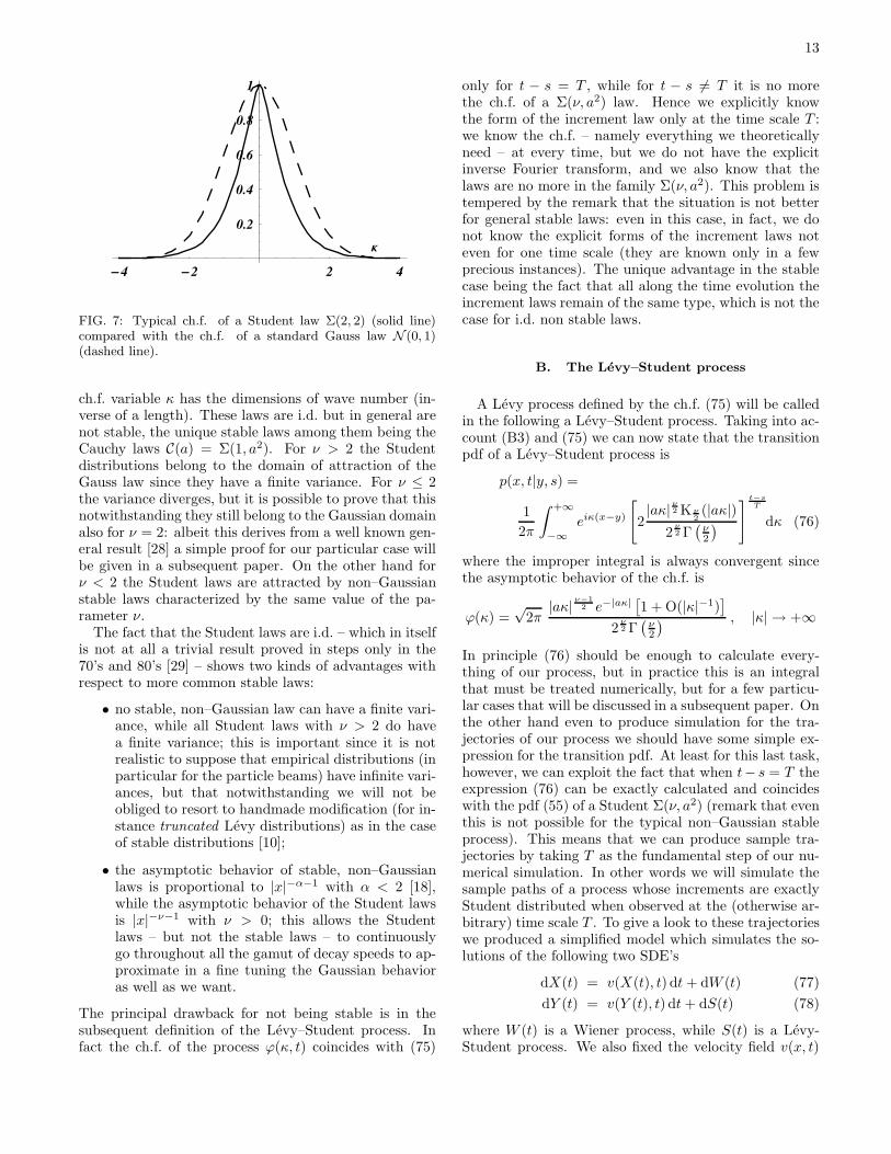
13

-4 -2 2 4

0.2

0.4

0.6

0.8

1

Κ

FIG. 7: Typical ch.f. of a Student law Σ(2, 2) (solid line)compared with the ch.f. of a standard Gauss law N (0, 1)(dashed line).

ch.f. variable κ has the dimensions of wave number (in-verse of a length). These laws are i.d. but in general arenot stable, the unique stable laws among them being theCauchy laws C(a) = Σ(1, a2). For ν > 2 the Studentdistributions belong to the domain of attraction of theGauss law since they have a finite variance. For ν ≤ 2the variance diverges, but it is possible to prove that thisnotwithstanding they still belong to the Gaussian domainalso for ν = 2: albeit this derives from a well known gen-eral result [28] a simple proof for our particular case willbe given in a subsequent paper. On the other hand forν < 2 the Student laws are attracted by non–Gaussianstable laws characterized by the same value of the pa-rameter ν.

The fact that the Student laws are i.d. – which in itselfis not at all a trivial result proved in steps only in the70’s and 80’s [29] – shows two kinds of advantages withrespect to more common stable laws:

• no stable, non–Gaussian law can have a finite vari-ance, while all Student laws with ν > 2 do havea finite variance; this is important since it is notrealistic to suppose that empirical distributions (inparticular for the particle beams) have infinite vari-ances, but that notwithstanding we will not beobliged to resort to handmade modification (for in-stance truncated Levy distributions) as in the caseof stable distributions [10];

• the asymptotic behavior of stable, non–Gaussianlaws is proportional to |x|−α−1 with α < 2 [18],while the asymptotic behavior of the Student lawsis |x|−ν−1 with ν > 0; this allows the Studentlaws – but not the stable laws – to continuouslygo throughout all the gamut of decay speeds to ap-proximate in a fine tuning the Gaussian behavioras well as we want.

The principal drawback for not being stable is in thesubsequent definition of the Levy–Student process. Infact the ch.f. of the process ϕ(κ, t) coincides with (75)

only for t − s = T , while for t − s 6= T it is no morethe ch.f. of a Σ(ν, a2) law. Hence we explicitly knowthe form of the increment law only at the time scale T :we know the ch.f. – namely everything we theoreticallyneed – at every time, but we do not have the explicitinverse Fourier transform, and we also know that thelaws are no more in the family Σ(ν, a2). This problem istempered by the remark that the situation is not betterfor general stable laws: even in this case, in fact, we donot know the explicit forms of the increment laws noteven for one time scale (they are known only in a fewprecious instances). The unique advantage in the stablecase being the fact that all along the time evolution theincrement laws remain of the same type, which is not thecase for i.d. non stable laws.

B. The Levy–Student process

A Levy process defined by the ch.f. (75) will be calledin the following a Levy–Student process. Taking into ac-count (B3) and (75) we can now state that the transitionpdf of a Levy–Student process is

p(x, t|y, s) =

1

2π

∫ +∞

−∞

eiκ(x−y)

[2|aκ| ν

2 K ν

2(|aκ|)

2ν

2 Γ(

ν2

)] t−s

T

dκ (76)

where the improper integral is always convergent sincethe asymptotic behavior of the ch.f. is

ϕ(κ) =√

2π|aκ| ν−1

2 e−|aκ|[1 + O(|κ|−1)

]

2ν

2 Γ(

ν2

) , |κ| → +∞

In principle (76) should be enough to calculate every-thing of our process, but in practice this is an integralthat must be treated numerically, but for a few particu-lar cases that will be discussed in a subsequent paper. Onthe other hand even to produce simulation for the tra-jectories of our process we should have some simple ex-pression for the transition pdf. At least for this last task,however, we can exploit the fact that when t− s = T theexpression (76) can be exactly calculated and coincideswith the pdf (55) of a Student Σ(ν, a2) (remark that eventhis is not possible for the typical non–Gaussian stableprocess). This means that we can produce sample tra-jectories by taking T as the fundamental step of our nu-merical simulation. In other words we will simulate thesample paths of a process whose increments are exactlyStudent distributed when observed at the (otherwise ar-bitrary) time scale T . To give a look to these trajectorieswe produced a simplified model which simulates the so-lutions of the following two SDE’s

dX(t) = v(X(t), t) dt+ dW (t) (77)

dY (t) = v(Y (t), t) dt+ dS(t) (78)

where W (t) is a Wiener process, while S(t) is a Levy-Student process. We also fixed the velocity field v(x, t)

14

0.5 1 1.5 2

0.1

0.2

0.3

0.4

0.5

0.6

0.7

x

pro

babil

ity

den

sity

fun

ctio

ns

FIG. 8: The pdf’s of the increments for the Gaussian pro-cesses (SDE (77), dashed line; σ ≃ 0.53) and for the Levy–Student process with law Σ(4, 1) (SDE (78), solid line; σ ≃

0.71). The parameters are chosen so that the two pdf’s havethe same modal values and similar shapes.

-8

-6

-4

-2

2

4

6

FIG. 9: Typical trajectory of a stationary, Gaussian(Ornstein–Uhlenbeck) process X(t) (see SDE (77)). To com-pare it with the Student trajectory, the vertical scale has beenset equal to that of FIG. 10

in a suitable way: it will not depend on time t, and itsvalue is (for given b > 0 and q > 0)

v(x) = −bxH(q − |x|)

where H is the Heaviside function. This flux will at-tract the trajectory toward the origin when |x| ≤ q,and will allow the movement to be completely free for|x| > q. The forms of the typical pdf’s used in our sim-ulations are shown in FIG. 8. In a simplified model fora collimated beam this will then produce a stationary,Ornstein–Uhlenbeck process for the SDE (77) if the in-tensity of the Gaussian noise is not too large. The pro-cess solution of the SDE (78) will instead have differentcharacteristics. Let us suppose to fix the ideas that thetwo parameters defining the velocity field are b = 0.35and q = 10. The FIG. 9 displays a typical trajectoryof a 104 steps solution X(t) of (77) when the varianceof the Gaussian distributed increments is σ2 = 0.28. In

-8

-6

-4

-2

2

4

6

FIG. 10: Typical trajectory of a stationary, Student processY (t) (see EDS (78), ν = 4 and a = 1).

our simplified 1–DIM model of the transverse dynamicsof a particle beam this means that the trajectories al-ways stay inside the beam core. Let us then take as lawfor the increments of (78) a Student distribution Σ(4, 1):its pdf looks not very different from that of the previ-ous Gaussian distribution, as the FIG. 8 clearly show.That notwithstanding the process Y (t) differs in severalrespects from X(t). Indeed not only the typical trajec-tory displayed in FIG. 10 shows a wider dispersion of itsvalues and a few larger spikes. The principal difference israther in the fact that while the trajectories of X(t) showa remarkable stability in their statistical behavior, thepaths of Y (t) have the propensity to make occasional ex-cursions far away from the beam core (see FIG. 11), andseldom they also definitely drift away from the core (seeFIG. 12). This depends of course on the mentioned prop-erties of the trajectories of a non–Gaussian Levy process,and in particular on the fact that they are only stochas-tically, and not pathwise continuous, namely that theycontain occasional jumps. The frequency and the size ofthese jumps can also be fine tuned by suitably choosingthe values of the parameters of the law Σ(ν, a2) of theincrements. It is this feature of a Levy–Student processthat suggests to adopt this model to describe the rareescape of particles away from the beam core.

VI. CONCLUSIONS

In the previous sections we have introduced the Stu-dent laws in our SM model for the particle beam dy-namics first of all in order to make use of their featuresdepending on their enhanced variance. In particular wehave shown that the longer tails with respect to the sim-ilar Gaussian distributions can help to account for thefinding of a larger than expected number of particles re-moved far away from the beam core.

It should be remarked, however, that all along the Sec-tion IV our processes were Gaussian processes since theunderlying SDE (1) is still powered by a Brownian noise.

15

-5

5

10

15

20

FIG. 11: Occasional trajectory of a stationary, Student pro-cess Y (t) (see EDS (78), ν = 4) with a temporary excursionout of the core.

-100

-80

-60

-40

-20

FIG. 12: Rare, but possible trajectory of a stationary, Stu-dent process Y (t) (see EDS (78), ν = 4): here the particledefinitely drifts away from the core.

This is true even in the Section IV B where we first intro-duced the Student laws (55) as stationary distributionsof the process. It is only in the Section V that we in-troduced a new kind of SDE with a Levy–Student noise.The more relevant feature of these processes is the factthat their trajectories make jumps: indeed this can be-come a model for the halo formation in the beams. Froma physical point of view these jumps can be produced byoccasional hard collisions among the beam particles, theprobability of these collisions growing with the intensityof the beam. In some sense it is not only the varianceof the transverse distribution of the beam which princi-pally rules the emergence of a halo: in the simulationsproduced here the variances of the Gaussian and of theStudent processes were roughly the same. Rather it isthe qualitative character of the process which accountsfor the rare escape of the particles from the beam core.For a process produced by a Gaussian noise (a processpathwise continuous: almost every trajectory is every-where continuous) there is no chance to observe trajecto-ries going out of a well collimated beam. On the contrary,

for a process produced by a Levy–Student noise (a pro-cess only stochastically continuous: trajectories can havejumps) occasionally the jump is large enough to put theparticle out of the stream. Of course the frequency andthe size of these jumps depend on the parameters ν anda of the process: the jumps tend to be smaller and lessfrequent when the Σ(ν, a2) distributions approximate aGaussian law. In our opinion it would be very interest-ing to explore the possibility that the processes under-lying the intense beam dynamics be ruled by some sortof Levy–Student noise rather than by the usual Gaus-sian noise. It is then important to point out that a fewnumerical evidences [20] begin to emerge which confirmthis conjecture.

These remarks point to several research directions.First of all it is important to better study the Levy–Student process in itself: for example a knowledge of theLevy–Khintchin functions of the Student laws would berelevant to the fine tuning of the frequency and the sizeof the trajectory jumps. On the other hand even the dif-ferential form of its Chapman–Kolmogorov equation [30]would be instrumental to discuss the time evolution ofthe process. Then it must be remarked that at presentwe have just defined the Levy–Student process, but weadded no dynamics: it is as if we have the Wiener pro-cess, but no Stochastic Mechanics or any other dynamicalmodel added to this kinematics. In other words we needto build a new generalized SM for the Levy–Student pro-cesses. Finally it would be important at this point tohave empirical or numerical data able to corroborate thehypothesis that the increments of the transverse variablesof a beam are in fact distributed according to a Studentlaw, rather than according to the usual Gaussian law.

Acknowledgments

We would like to thank Dr. C. Benedetti, Prof. F.Mainardi, Prof. G. Turchetti and Dr. A. Vivoli for usefulcomments and suggestions.

APPENDIX A: INFINITELY DIVISIBLE AND

STABLE LAWS

The relevant mathematical concepts used in this paperare better discussed in the framework of the theory of theaddition of independent random variables (r.v.): for moredetails see [31, 32, 33]. In the following we will describethe law L of a r.v. X by giving her characteristic function(ch.f.)

ϕ(κ) = E(eiκX)

where E(·) is the expectation under the law L. When Lhas a pdf f(x), then ϕ(κ) is just its Fourier transform. Itis well known that the law L of the sum of n independentr.v.’s with laws L1, . . . ,Ln has a ch.f. which is the product

16

of the ch.f.’s of the component laws:

ϕ(κ) = ϕ1(κ) · . . . · ϕn(κ) (A1)

On the other hand we say that a law L is decomposed

in the laws L1, . . . ,Ln when its ch.f. can be written asa product (A1) of the ch.f.’s of its components. Thisalready allows us to introduce two fundamental concepts:a law L with ch.f. ϕ is said to be i.d. when for every nthere is a law Ln with ch.f. ϕn such that ϕ = ϕn

n. In otherwords this means that for every n a r.v. X with law Lcan always be decomposed in the sum of n independentr.v.’s all with the same law Ln (identically distributed).Remark, however, that in general the laws Ln are notof the same type as L. Let us remember here that wesay that two laws are of the same type when we get onefrom the other by means of a centering and a rescaling;in other words, if ϕ(κ) in a ch.f., then all the ch.f.’s of thesame type have the form eiaκϕ(bκ) for every a and b > 0.For instance all the Gaussian laws N (µ, σ2) belong to thesame (Gaussian) type; on the contrary the Poisson lawsP(λ) with different values of λ do not belong to the sametype. Now, a law L is said to be stable when it is i.d.and the component laws are of the same type as L. Moreprecisely a ch.f. ϕ(κ) is stable when for every b, b′ > 0there exist a and c such that

ϕ(cκ) = eiaκϕ(bκ)ϕ(b′κ) .

As an example: the Gaussian and the Cauchy laws arestable; the Poisson laws are instead only i.d. The fami-lies of i.d. and stable laws are completely characterized:in fact the celebrated Levy–Khintchin formula gives themore general form for the ch.f.’s of these two classes;however, while in the case of the stable laws these ch.f.’s(albeit not in general the laws themselves) are explicitlyknown in terms of elementary functions, for the i.d. lawsthe ch.f.’s are given through an integral containing a func-tion L(x) (Levy function) associated to every particularlaw. But for a few classical cases the Levy functions ofthe i.d. laws are not known.

APPENDIX B: CENTRAL LIMIT THEOREM

AND LEVY PROCESSES

Let us consider the sequence of r.v.’s Xn,k with n ∈ N

and k = 1, . . . , n with Xn,1, . . . , Xn,n independent forevery n. The modern formulation of the Central LimitProblem asks to find the more general laws which arelimits of the laws of the consecutive sums

Sn =

n∑

k=1

Xn,k (B1)

Remark that these sums generalize the usual partial sumsof the classical Central Limit Theorem in that: when wego from Sn to, say, Sn+1, the first n terms do not in gen-eral remain the same: for example Xn.1 does not coincide

with Xn+1.1. Under very general technical conditions theCentral Limit Theorem now states that the family of allthe limit laws of the consecutive sums (B1) coincides withthe family of i.d. laws. The stable laws come into playonly when we specialize the form of our consecutive sums:when we have

Xn,k =Xk

an− bnn

where an and bn are sequences of numbers, and Xk areindependent r.v.’s, the consecutive sums take the form ofthe usual normed sums (centered and rescaled sums ofindependent r.v.’s)

Sn =S∗

n

an− bn , S∗

n =

n∑

k=1

Xk . (B2)

Then, if theXk are also identically distributed, the familyof the limit laws of the normed sums (B2) coincides withthe family of the stable laws. The classical (Gaussian)Central Limit Theorem is an example of convergence to-ward a stable law; on the other hand the Poisson Theo-rem (convergence of Binomial laws toward Poisson laws)is an example of convergence toward an i.d. law. Everystable law has its own domain of attraction, namely theset of laws attracted by it in the sense of the convergenceof normed sums (B2) of independent r.v.’s all distributedas the attracted law. It can be proved that all the lawswith finite variance are in the domain of attraction of theGauss law, and that a law can be attracted by a non–Gaussian stable law only if it has infinite variance.

The general formulation of the Central Limit Theo-rem is strictly connected to the definition of the pro-cesses with independent increments (decomposable pro-

cesses). It is apparent in fact that if the increments∆X(t) = X(t + ∆t) − X(t) for non superposed inter-vals are independent, the previous forms of the CentralLimit Theorem imply that the laws of the incrementsmust be i.d. laws. Moreover, since the decomposableprocess are also Markov processes, the laws of the in-crements are also all that is needed to completely definethem. If a decomposable processes X(t) is stationary

(namely the law of X(t+ s) −X(s) does not depend ons) and stochastically continuous (namely for every t wehave X(t+ ∆t)−X(t) → 0 in probability when ∆t→ 0)we will call it a Levy process. Remark that a Poisson pro-cess is a Levy process since, despite its discontinuities, itis stochastically continuous. In fact these discontinuitiesdo not impair the stochastic continuity of the process be-cause they are moving (as opposed to fixed) discontinu-ities. On the other hand it is possible to prove that onlythe Gaussian Levy processes (for example the Wiener, orthe Ornstein–Uhlenbeck processes) are pathwise contin-

uous, namely: almost every sample path is everywherecontinuous (there are not even moving discontinuities).Now, if ϕ(κ) is the ch.f. of an i.d. law and T is a suit-able time constant, it is possible to prove that [ϕ(κ)]∆t/T

is the ch.f. of the increments ∆X(t) of a Levy process.

17

Hence, if the process has a pdf, the stationary transitionpdf is

p(x, t|y, s) =1

2πPV

∫ +∞

−∞

eiκ(x−y)[ϕ(κ)]t−s

T dκ (B3)

so that, at least in principle, we know all that is neededto define the process.

The sample paths of a Levy process are also well char-acterized: it is possible in fact to prove that almost alltrajectories are bounded and are continuous with the ex-ception of a countable set of moving jumps (first kind

discontinuities). Then, let us suppose that Lt(x) is theLevy–Khintchin function of the i.d. law of the incrementX(s + t) − X(s): if νt(x) is the random number of thejumps in [s, s+ t) of height in absolute value larger thanx > 0, it is possible to prove that

|Lt(x)| = E(νt(x))

so that the Levy–Khintchin function of an i.d. law playsalso the role of a measure of the frequency and height ofthe trajectory jumps.

[1] N. Cufaro Petroni, S. De Martino, S. De Siena, and F.Illuminati, Phys. Rev. ST Accel. Beams 6, 034206 (2003);N. Cufaro Petroni, S. De Martino, S. De Siena and F.Illuminati, in Quantum aspects of beam physics 2003, P.Chen et al. eds. (World Scientific, Singapore, 2004) p. 36.

[2] N. Cufaro Petroni, S. De Martino, S. De Siena and F.Illuminati, in Proceedings of the European particle accel-erator conference – EPAC04 (EPS–AG/CERN 2004), p.2056.

[3] H. Koziol, Los Alamos M. P. Division Report No. MP-3-75-1 (1975).

[4] M. Reiser, C. Chang, D. Kehne, K. Low, T. Shea, H.Rudd, and J.Haber, Phys. Rev. Lett. 61, 2933 (1988).

[5] R.L. Gluckstern, Phys. Rev. Lett. 73, 1247 (1994); R.L.Gluckstern, W.-H. Cheng and H.Ye, Phys. Rev. Lett.75, 2835 (1995); R.L. Gluckstern, W.-H. Cheng, S.S.Kurennoy, and H.Ye, Phys. Rev. E 54, 6788 (1996); H.Okamoto and M. Ikegami, Phys. Rev. E 55, 4694 (1997);R.L. Gluckstern, A.V. Fedotov, S.S. Kurennoy, and R.Ryne, Phys. Rev. E 58, 4977 (1998); T.P. Wangler, K.R.Crandall, R. Ryne, and T.S. Wang, Phys. Rev. ST-AB1, 084201 (1998); A.V. Fedotov, R.L. Gluckstern, S.S.Kurennoy, and R.Ryne, Phys. Rev. ST-AB 2, 014201(1999); M. Ikegami, S. Machida, and T. Uesugi, Phys.Rev. ST-AB 2, 124201 (1999); Quiang and R. Ryne,Phys. Rev. ST-AB 3, 064201 (2000).

[6] O. Boine-Frankenheim and I. Hofmann Phys. Rev. ST–AB 3, 104202 (2000); L. Bongini, A. Bazzani, G.Turchetti, and I. Hofmann Phys. Rev. ST–AB 4, 114201(2001); A.V. Fedotov and I. Hofmann Phys. Rev. ST–AB5, 024202 (2002).

[7] T. Wangler, RF linear accelerators, (J. Wiley, New York,1998)

[8] L.D. Landau and E.M. Lifchitz, Cintique physique, (MIR,Moscow, 1990).

[9] F. Ruggiero, Ann. Phys. (N.Y.) 153, 122 (1984); F. Rug-giero, E. Picasso and L.A. Radicati, Ann. Phys. (N. Y.)197, 396 (1990); J. Struckmeier, Phys. Rev. ST–AB 3,034202 (2000).

[10] W. Paul and J. Baschnagel, Stochastic Processes: FromPhysics to Finance, (Springer, Berlin, 2000)

[11] E. Nelson, Dynamical theories of Brownian motion(Princeton University Press, Princeton N. J., 1967);E. Nelson, Quantum Fluctuations (Princeton UniversityPress, Princeton N. J., 1985).

[12] F. Guerra, Phys. Rep. 77, 263 (1981).[13] F. Guerra and L. M. Morato, Phys. Rev. D 27, 1774

(1983).[14] S. Albeverio, Ph. Blanchard and R. Høgh-Krohn, Expo.

Math. 4, 365 (1983).[15] R. Fedele, G. Miele and L. Palumbo, Phys. Lett. A 194,

113 (1994), and references therein; S.I. Tzenov, Phys.Lett. A 232, 260 (1997).

[16] S.A. Khan and M. Pusterla, Eur. Phys. J. A 7, 583(2000).

[17] L. Morato, J. Math. Phys. 23 (1982) 1020.[18] R.N. Mantegna and H.E. Stanley, An Introduction to

Econophysics (Cambridge U.P. 2000)[19] C.K. Allen, K.C.D. Chan, P.L. Colestock, K.R. Crandall,

R.W. Garnett, J.D. Gilpatrick, W. Lysenko, J. Qiang,J.D. Schneider, M.E. Schulze, R.L. Sheffield, H.V. Smithand T.P. Wangler, Phys. Rev. Lett. 89 (2002) 214802.

[20] A. Vivoli, C. Benedetti and G. Turchetti, Time SeriesAnalysis of Coulomb Collisions in a Beam DynamicsSimulation, Workshop COULOMB’05, September 12–16,2005, Senigallia.

[21] S. De Martino, S. De Siena, and F. Illuminati, PhysicaA 271, 324 (1999); N. Cufaro Petroni, S. De Martino,S. De Siena, and F. Illuminati, Phys. Rev. E 63, 016501(2000); N. Cufaro Petroni, S. De Martino, S. De Sienaand F. Illuminati, in Quantum aspects of beam physics2K, P. Chen ed. (World Scientific, Singapore, 2002) p.507.

[22] N. Cufaro Petroni, S. De Martino, S. De Siena, and F.Illuminati, Int. J. Mod. Phys. B 18, 607 (2004)

[23] E. Madelung, Z. Physik 40, 332 (1926); D. Bohm, Phys.Rev. 85, 166, 180 (1952).

[24] N. Cufaro Petroni, S. De Martino, S. De Siena, and F. Il-luminati, J. Phys. A 32, 7489 (1999); N. Cufaro Petroni,S. De Martino, S. De Siena and F. Illuminati, in Quan-tum aspects of beam physics 1998, P. Chen ed. (WorldScientific, Singapore, 1999) p. 710; N. Cufaro Petroni, S.De Martino, S. De Siena, R. Fedele, F. Illuminati and S.I. Tzenov, in Proceedings of the European particle accel-erator conference – EPAC98, S. Myers et al. eds. (IoPPublishing, Bristol, 1998), p. 1259.

[25] N. Cufaro Petroni and F. Guerra, Found. Phys. 25, 297(1995); N. Cufaro Petroni, in Quantum Communicationsand Measurement, V.P. Belavkin et al. eds. (Plenum,New York, 1995), p. 43; N. Cufaro Petroni, S. De Mar-tino and S. De Siena, in New Perspectives in the Physicsof Mesoscopic Systems, S. De Martino et al. eds. (WorldScientific, Singapore 1997) p. 59.

[26] N. Cufaro Petroni, S. De Martino and S. De Siena, Phys.

18

Lett. A 245, 1 (1998).[27] L.D. Landau and E.M. Lifchitz, Mecanique Quantique,

(MIR, Moscow, 1988).[28] J.-P. Bouchaud and A. Georges, Phys. Rep. 195, 127

(1990).[29] E. Grosswald, Ann. Prob. 4, 680 (1976); E. Grosswald,

Z. Wahrsch. 36, 103 (1976); M.E.H. Ismail, Ann. Prob.5, 582 (1977); L. Bondesson, Ann. Prob. 7, 965 (1979); J.Pitman and M. Yor, in Stochastic Integrals (D. Williamseditor), L. N. Math. 851, 285 (Springer, 1981); L. Bon-desson, Generalized Gamma Convolutions and RelatedClasses of Distributions and Densities, L. N. Stat. 76

(Springer, 1992); J. Pitman, Electr. J. Prob. 4 (1999)paper 11.

[30] C.W. Gardiner, Handbook of Stochastic Methods(Springer, 1997).

[31] M. Loeve, Probability Theory I and II (Springer, 1977and 1978).

[32] W. Feller, An Introduction to Probability Theory and ItsApplications I and II (J. Wiley & Sons, 1968 and 1971).

[33] B.V. Gnedenko and A.N. Kolmogorov, Limit dis-tributions for sums of independent random variables(Addison–Wesley, 1968).