FORECASTING METHODS OF NON-STATIONARY STOCHASTIC

PROCESSES THAT USE EXTERNAL CRITERIA

Igor V. Kononenko, Anton N. Ryepin

National Technical University “Kharkiv Polytechnic Institute”, Ukraine

1. Introduction

While forecasting the development of socio-economic systems there often

arise the problems of forecasting non-stationary stochastic processes having a

scarce number of observations (5-30), while the repeated realizations of processes

are impossible.

To solve such problems there have been suggested a number of methods, in

which unknown parameters of the model are estimated not at all points of time

series, but at a certain subset of points, called a learning sequence. At the

remaining points not included in the learning sequence and called the check

sequence, the suitability of the model for describing the time series is determined.

These methods include the method of cross-validation and Group method of data

handling (GMDH) proposed by Alexey G. Ivahnenko. The disadvantage of these

methods is that a certain combination of data partitions is set in advance and it does

not take into account the specifics of the task.

2. Purpose of work

The purpose of this work is to create and study an effective forecasting

method of non-stationary stochastic processes in the case when observations in the

base period are scarce.

3. H-criterion method (I. Kononenko, 1982)

The data including retrospective information can be presented in a form of

matrix Г ir , , qr ,1 , ni ,1 , where q – number of significant variables including

2

the predicted variable; n – number of points in the time base of forecast;

),...,,( ,12,11,1 n - vector of values of the predicted variable.

The list of elementary models is formed. It includes different mathematical

models, which by hypothesis can be included in the final forecasting model. The

elementary power, exponential, logarithmic, trigonometric, rational and other

functions are used. From the models in the list the linear combinations of 1,2,...,M

models are formed comprising the set of test models. For each test model the

estimation of its suitability for forecasting is made.

The matrix Г is further divided into two submatrices – learning submatrix Г L

and check submatrix Г C. The division is made by means of selecting the first n/2

columns of matrix Г as Г L and the remaining columns as Г C. If n is odd then (n–

1)/2 columns should be selected. The parameters of all formed models are

estimated using the learning submatrix

LG,ρηˆ jA , (1)

where jA – the vector of estimated parameters for j-th model,

Tpj aaaA ,,, 21)( ; jA – the vector of estimates for jA ; – the vector of weighting

coefficients considering the error variance or importance i1γ for building the

model, L,1 Ni , L

ρ,,ρ,ρρ 21 N ; (…) – function that is set analytically or

algorithmically. The estimation of parameters is made by methods most

appropriate for the situation at hand. When choosing a method the following

criteria must be taken into account: the kind of test models, the existing

assumptions about additivity and multiplicativity of errors, about the error

distribution law, about the class it might belong to, about the error correlation and

other information.

The loss-function F() is selected according to the available information

about the error distribution law or the class of such laws.

After the estimation of parameters of all test models according to formula (1)

for each j-th model at all points of past history we calculate

3

,))ˆ,((1

)()(11

n

i

jjijii AFF (2)

where i – weighting coefficient; F() – loss-function, selected according to

the available information about the distribution law of errors i or the class of such

laws. Then ГC is used as a learning submatrix, and ГL as a check one, and for all

models the process of parameters estimation and calculation of 2 values is

repeated.

In the matrix Г new learning and check submatrices are chosen. The number

of rows in ГL is decreased by one. The process of estimation of model parameters

and calculation of 3 is repeated, the learning submatrix is used as the check one

and the check submatrix - as the learning one, 4 is calculated and similarly we

continue using the bipartitioning. The process is stopped after a set number of

iteration g. Among test models estimated by different methods the one with the

minimum value of H-criterion is selected.

gH 21 . (3)

The obtained model is used for forecasting.

4. Bootstrap evaluation method (I. Kononenko, 1990)

The data including retrospective information can be presented in a form of

matrix ,,ijG ,q,1j ,n,1i where q – number of significant variables

including the predicted variable, n – volume of past history, n,12,11,1 ,...,, –

vector of values of the predicted variable.

Let 1L , where L – the number of a model in the set of test models. Let the

model BN ,f iL be tested for the description of the observed process, i.e. we get

the expression iiL

i,1 ,f BN , where Ni – vector of independent variables, B

– vector of estimated parameters, i – independent errors having the same and

symmetrical density of distribution, n,1i .

4

1. The parameters of the model BNi ,f L we estimate using matrix G

basing on the condition

n

1ii

Li,1 ,,fFminargˆ BNB

B

where iF – loss function, BN ,f iL

i,1i , n,1i . The loss function is

selected depending on the available assumptions about the errors additively

imposed on the true model. Thus, F or .F2

For the model

BN ˆ,f iL we determine the deviation from points of G, BN ˆ,, i

Li1i fbias ,

n,1i . Numbers biasi form the BIAS vector.

2. We divide the matrix G into two submatrices – learning submatrix GL and

check submatrix GC. We include first n-1 columns of matrix G in submatrix GL and

n-th column in GC. The learning submatrix has the following form LG i,j ,

q,1j , 1n,1i , and the check one – cG n,j , q,1j .

Using the learning submatrix GL we estimate the parameters B of the test

model by the above mentioned method and obtain 0B as a result. Basing on the

check submatrix we calculate the deviation of the model from the statistics

20n

Ln1

L0 fD BN ˆ,, .

Let k=1, where k – number of iteration, which performs the bootstrap

evaluation.

3. We perform bootstrap evaluation, which consists in the following. We

randomly (with equal probability) select numbers from the BIAS vector and add

them to the values of model BN ˆ,f iL . As a result we obtain “new” statistics k

i,1 ,

n,1i , which looks like the following

siLk

i,1 biasˆ,f BN , n,1i , n,...,2,1s .

5

Then we divide the matrix Gk (a new one this time) into GL,k and GC,k. We

estimate the unknown parameters basing on GL,k as earlier and calculate the model

deviation from GC,k

2kn

Lkn1

Lk fD BN ˆ,, .

4. If k<K-1 then we suppose that k:=k+1 and return to step 3 (where K –

number of bootstrap iterations), otherwise proceed to step 5.

5. We evaluate

1N

0k

Lk

L DD .

6. If L<z then we suppose that L:=L+1 and move to step 1 (where z –

number of models in the list), otherwise we stop.

The model with minimal DL is considered to be the best one.

5. The analysis of forecasting methods

A computational analysis of the suggested forecasting methods has been

performed. The following mathematical models have been chosen for the analysis:

3x2xy 2 , 3x6xy 2 , 3x8x2y 2 , 3x16xy 2 ,

11x6xy 2 , 11x2xy 2 , 27x16x2y 2 , 27x8x2y 2 ,

hereinafter referred to as true models. On each of these models defined at points

i1,0x i , 10,1i we imposed an additive noise ),0(N~ 2 , where

9)10yy(3.010

1i

10

1iii

,

where iy – value of the model at point ix , 10,1i , and then defined the best

forecasting model by means of the suggested methods. The loss function of the

form 2)()(F was chosen as it is the most frequently used in practice.

During the analysis we considered all combinations of one, two, three functions

from the list 21

x , x , 23

x , 2x , 25

x , 3x , 1x , 21

x

, 23

x

in form of their linear

combinations. We analyzed the properties of the method when forecasting on d

6

points, 10,5,3,2,1d . For every forecasting model obtained we calculated the

following characteristics:

- Relative percent mean absolute deviation (PMAD) evaluated at the

estimation period

10

1ii

10

1iii zyz ;

where iii yz , iy – value of the obtained forecasting model at point i, 10,1i ;

- Percent mean absolute deviation (PMAD) evaluated at the estimation

period

10

1ii

10

1iii yyyE ;

- Percent mean absolute deviation (PMAD) evaluated at the forecasting

period

d

11ii

d10

11iiid yyy1E ;

- Relative mean squared error (MSE) evaluated at the forecasting period

d10

11i

2ii

md yz

d

1D ;

- Mean squared error (MSE) evaluated at the forecasting period

d10

11i

2ii

td yy

d

1D .

The analysis is performed on 1000N realizations of noise.

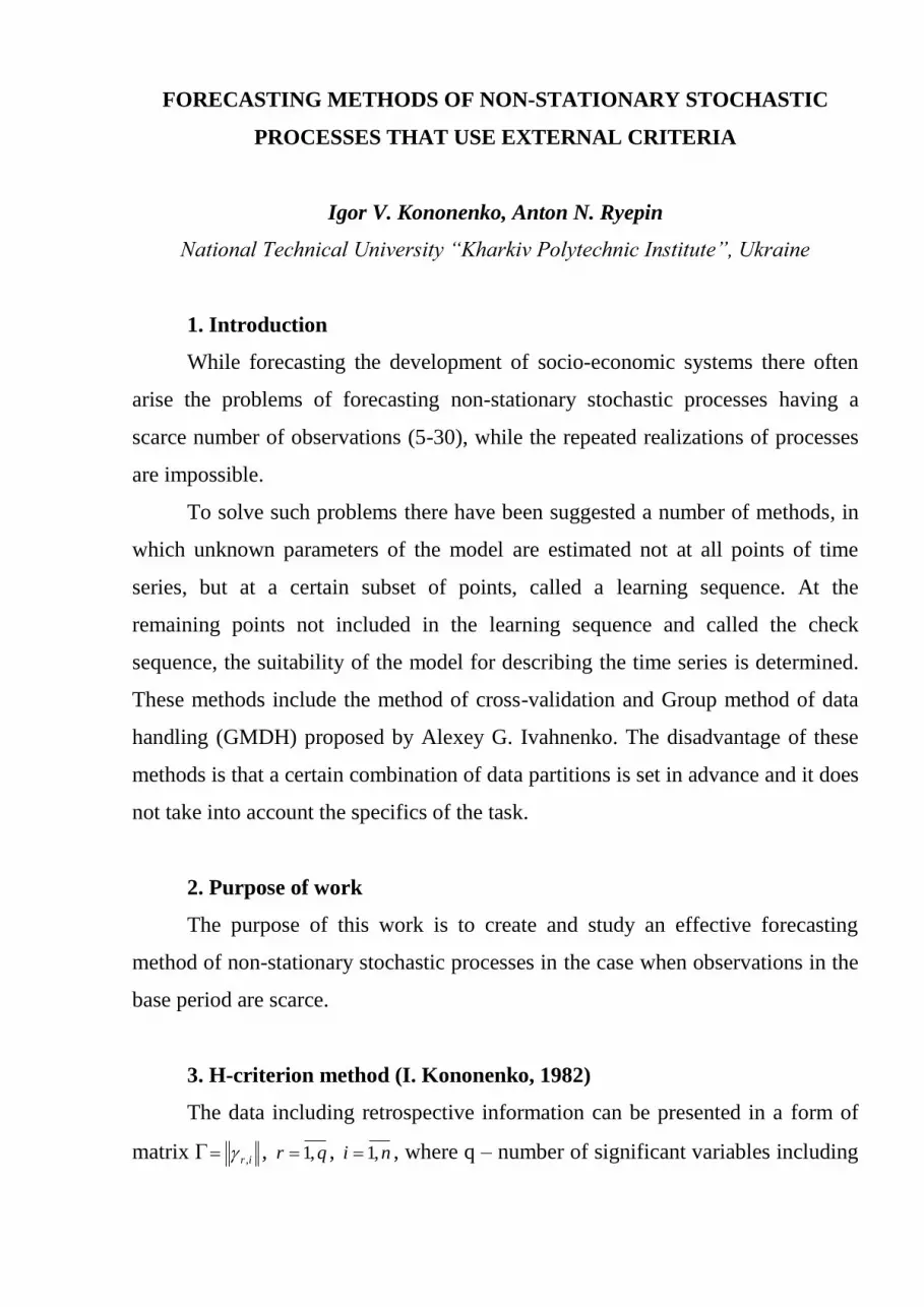
For the H-criterion method, the division of data into learning and checking

submatrices was done in accordance with the rules determined by the matrices

7

21212121

21212121

21212121

21212121

21211221

12211221

12121221

12121212

12121212

12121212

1R ,

12121212

12121212

12121212

12121212

12211212

12211221

12212121

21212121

21212121

21212121

2R ,

2111111111

1211111111

1121111111

1112111111

1111211111

1111121111

1111112111

1111111211

1111111121

1111111112

3R ,

1221112112

1112121111

2121221121

1211111121

2121221212

2121222111

1222121112

1111112111

2112221122

2121211212

4R .

Every j-th column of the matrix 4,1, dRd corresponds to the j-th method of

data division, 8,1j for R1, R2 and 10,1j for R3, R4. Every )(dijr -th element of

matrix Rd 10,1j determines, into which submatrix – learning (GL) or checking

(GC) – goes i-th point of history. Here 1)( dijr means that the point is used in

submatrix GL, )(dijr = 2 means that the point is used in submatrix GC.

Matrix R3 corresponds to the cross-validation procedure that served as the

source for comparison.

Matrix R4 is the randomly generated matrix.

For the bootstrap evaluation method the number of bootstrap iterations was

selected from 10, 20 to 50.

We calculated:

- Average (across noise realizations) relative percent mean absolute

deviation (PMAD) evaluated at the estimation period

N

1kk

N

1;

- Average (across noise realizations) percent mean absolute deviation

(PMAD) evaluated at the estimation period

N

1kkE

N

1E ;

8

- Average (across noise realizations) percent mean absolute deviation

(PMAD) evaluated at the forecasting period

N

k

dkd EN

E1

11

1 ;

- Average (across noise realizations) relative mean squared error (MSE)

evaluated at the forecasting period

N

1k

mdk

md D

N

1D ;

- Average (across noise realizations) mean squared error (MSE) evaluated at

the forecasting period

N

1k

tdk

td D

N

1D ,

where k , kE , dk1E , mdkD and t

dkD – error values for k-th realization of noise,

N,1k . Confidence intervals of 95 percent have been estimated for , E , d1E ,

mdD and t

dD .

The comparison of the efficiency of the suggested methods and cross-

validation method has been made. Using the same analysis algorithm and the initial

data as for analysis of the suggested methods, the investigation of cross-validation

method has been conducted and the values of characteristics , E , 1E , mD , tD

were obtained, also 95% confidence intervals for these characteristics have been

built.

We compared the characteristics with the two-sample t-test assuming the

samples were drawn from the normally distributed populations, which in the

context of the considered problem has the following form

Q2Q,NVvP ,

where Q,NV – value defined by the table that corresponds to the significance

level of Q , v – value calculated by the following formula

N

ssv

22

21

,

9

where 21 , 1 and 2 – compared characteristics, 1s and 2s – estimates of

root-mean-square differences of 1 and 2 correspondingly, 1000N .

The significance level of Q is said to be equal to 2,5 %. For 5,2Q and

1000N 96,1, QNV .

The values of v calculated for pairs of compared characteristics (for H-

criterion method matrices R1, R4, R6 were selected) have been analyzed.

The values of characteristics of the suggested forecasting methods are

significantly less (with the 95% of confidence probability) at the forecasting period

than the values of characteristics of cross-validation method for all true models

considered and intervals of the forecasting period.

Figure 1 depicts how the PMAD dE1 , evaluated at the forecasting period

changes for mathematical model 3x2xy 2 depending on the number of

partitions g. In the given case d=10, i.e. the forecasting is performed at 10 points.

0,1

0,15

0,2

0,25

0,3

0,35

0,4

0,45

1 2 3 4 5 6 7 8 9 10

g

%

Matrix R1 Matrix R2 Matrix R3 - CV Matrix R4 - Random Bootstrap

Figure 1 - Percent mean absolute deviation (PMAD) evaluated at the

forecasting period

Having analyzed the given example we can draw a number of conclusions:

10

- when the number of partitions increases in case of using matrices R1 and R2

we observe the downward trend of dE1 with some fluctuations in this trend that

depend on the ways of data partition;

- the partition according to the cross-validation procedure, in which the

check points fall into the observation interval, produces significantly less accurate

forecasts. The comparison of the efficiency of different partitions with randomly

generated matrix R6 has shown that the reasonable choice of partition sequences

permits to get a more accurate longer-term forecast;

- the bootstrap evaluation method, which requires no learning or checking

matrices, produces the more accurate forecast than the cross-validation procedure

- the comparison of two suggested methods enables to state that the

bootstrap evaluation method makes it possible to obtain more accurate longer-term

forecasts as compared with H-criterion method only in case of a small number of

partitions. Otherwise the usage of selected matrices R1 and R2 permits to get more

accurate forecasts. Nevertheless, the bootstrap evaluation method turned out to be

more accurate than the H-criterion method when using matrix R6.

The similar chars can be observed for the remaining mathematical models

used in the analysis.

The number of bootstrap iterations reasonable for using in the corresponding

methods has been determined. In case of analyzed models the number of bootstrap

iterations that allowed to reduce PMAD evaluated at the forecasting period was 40.

By changing the number of bootstrap iterations from 10 to 40 the value of PMAD

decreased and reached its minimum at 40, and than started to increase as the

number of iterations reached 50.

Thus, we conclude that the suggested methods are more accurate in the

forecasting period than the cross-validation method. Such conclusion permits to

recommend them for forecasting of non-stationary stochastic processes when the

number of points in the base period is small.

The suggested bootstrap evaluation method has helped in solving the tasks

of forecasting the sales volume of wheel tractors in the USA and the production

11

volume of bread and bakery in Kharkiv region (Ukraine). The latest is shown on

the figure 2. It should be noticed, that the forecast was made in 2002 and was not

corrected since then. The mean relative error for the period 2003-2006 is 5,91 %.

0

50

100

150

200

1996 1997 1998 1999 2000 2001 2002 2003 2004 2005 2006 2007 2008

Thousand t

ons

Prehistory Actual Data Forecast

Figure 2 - Production volume of bread and bakery in Kharkiv region

When solving different forecasting problems it is important to determine the

appropriateness of using one of the methods. The analysis results have shown that

when the number of partitions is large the H-criterion method produces the more

accurate longer-term forecasts than the bootstrap evaluation method. However, in

the real-life problems the bootstrap evaluation method might turn out to be more

accurate in the number of cases. That is why it is recommended to use the given

methods together. In such case every result obtained by means of these methods

must be assigned some weight on the basis of the a priori estimates of the methods

accuracy. The final forecast will be received in the form the weighted average

value of individual forecasts.