Piecewise Stationary Modeling of RandomProcesses Over Graphs With an Application to

Traffic PredictionArman Hasanzadeh, Xi Liu, Nick Duffield and Krishna R. Narayanan

Department of Electrical and Computer EngineeringTexas A&M University

College Station, Texas 77840Email: {armanihm, duffieldng, krn}@tamu.edu, xiliu.tamu@gmail.com

Abstract—Stationarity is a key assumption in many statisticalmodels for random processes. With recent developments in thefield of graph signal processing, the conventional notion of wide-sense stationarity has been extended to random processes definedon the vertices of graphs. It has been shown that well-known spec-tral graph kernel methods assume that the underlying randomprocess over a graph is stationary. While many approaches havebeen proposed, both in machine learning and signal processingliterature, to model stationary random processes over graphs,they are too restrictive to characterize real-world datasets asmost of them are non-stationary processes. In this paper, to well-characterize a non-stationary process over graph, we proposea novel model and a computationally efficient algorithm thatpartitions a large graph into disjoint clusters such that theprocess is stationary on each of the clusters but independentacross clusters. We evaluate our model for traffic prediction ona large-scale dataset of fine-grained highway travel times in theDallas–Fort Worth area. The accuracy of our method is veryclose to the state-of-the-art graph based deep learning methodswhile the computational complexity of our model is substantiallysmaller.

Index Terms—Piecewise Stationary, Graph Clustering, GraphSignal Processing, Traffic Prediction

I. INTRODUCTION

Stationarity is a well-known hypothesis in statistics andsignal processing which assumes that the statistical charac-teristics of random process do not change with time [1].Stationarity is an important underlying assumption for many ofthe common time series analysis methods [2]–[4]. With recentdevelopments in the field of graph signal processing [5]–[7], the concept of stationarity has been extended to randomprocesses defined over vertices of graphs [8]–[11]. A randomprocess over a graph is said to be graph wide-sense stationary(GWSS) if the covariance matrix of the process and the shiftoperator of the graph, which is a matrix representation of thegraph (see Section II-B), have the same set of eigenvectors.

Incidentally, GWSS is the underlying assumption of spectralgraph kernel methods which have been widely used in machinelearning literature to model random processes over graphs[12]–[16]. The core element in spectral kernel methods isthe kernel matrix that measures similarity between randomvariables defined over vertices. This kernel matrix has the

same set of eigenvectors as the Laplacian matrix (or adjacencymatrix) while its eigenvalues are chosen to be a function ofeigenvalues of the Laplacian matrix (or adjacency matrix).Therefore, the kernel matrix and the shift operator of the graphshare eigenvectors which is the exact definition of GWSS.

While the stationarity assumption has certain theoretical andcomputational advantages, it is too restrictive for modelingreal-world big datasets which are mostly non-stationary. In thispaper, we propose a model that can deal with non-stationarycovariance structure in random processes defined over graphs.The method we deploy is a novel and computationally efficientgraph clustering algorithm in which a large graph is partitionedinto smaller disjoint clusters. The process defined over eachcluster is stationary and assumed to be independent from otherclusters. To the best of our knowledge, our proposed clusteringalgorithm, stationary connected subgraph clustering (SCSC),is the first method to address this problem. Our model rendersit possible to use highly-effective prediction techniques basedon stationary graph signal processing for each cluster [17].An overview of our proposed clustering algorithm is shown inFig. 1.

Our work is analogous to piecewise stationary modeling ofrandom processes in continuous space, which has been studiedin the statistics literature. However, these methods cannot beextended to graphs due to discrete nature of graphs or thefact that the definition of GWSS is not inclusive (SectionIII-A). For instance, to model a non-stationary spatial process,Kim et al. [18] proposed a Bayesian hierarchical model forlearning optimal Voronoi tessellation while Gramacy [19] pro-posed an iterative binary splitting of space (treed partitioning).Piecewise stationary modeling has also been explored in timeseries analysis which is mainly achieved by detecting changepoints [20], [21]. Recently, there has been an effort in graphsignal processing literature to detect non-stationary vertices(change points) in a random process over graph [22], [23],however, to achieve that, authors introduce another definitionfor stationarity, called local stationarity, which is different fromthe widely-used definition of GWSS.

We evaluate our proposed model for traffic prediction ona large-scale real-world traffic dataset consisting of 4764

arX

iv:1

711.

0695

4v4

[ee

ss.S

P] 7

Sep

201

9

...

...

ActiveComponentExtraction

time

StationaryConnectedSubgraphClustering

Dataset ActiveComponents

StationaryClusters

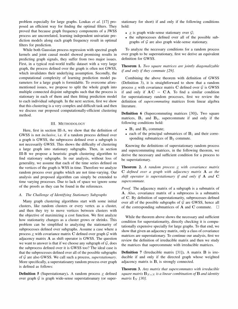
Fig. 1: An overview of our proposed stationary clustering algorithm. Given historical observation, i.e. time-series defined over nodes of agraph, first we extract active components. Next, our proposed stationary connected subgraph clustering (SCSC) tries to merge adjacent activecomponents to form stationary subgraphs.

road segments and time-series of average travel times oneach segment at a two-minute granularity over January–March2013. We use simple piecewise linear prediction models withineach cluster. The accuracy of our method is very close tothe state-of-the-art deep learning method, i.e. only 0.41%difference in the mean absolute percentage error for 10 minutepredictions, rising to 0.66% over 20 minutes. However, thelearning time of our proposed method is substantially smaller,being roughly 3 hours on a personal computer while the deeplearning method takes 22 hours on a server with 2 GPUs. Ourcontribution can be summarized as follows:• For the first time, we propose to model non-stationary

random processes over graphs with piecewise stationaryrandom processes. To that end, we propose a novelhierarchical clustering algorithm, i.e. stationary connectedsubgraph clustering, to extract stationary subgraphs ingraph datasets.

• We theoretically prove that the definition of GWSS is notinclusive. Hence, unlike many of the well-known graphclustering algorithms, adding one vertex at each trainingstep to clusters in an stationary clustering algorithm isbound to diverge. To address this issue, we propose touse active components as input to stationary clusteringalgorithm instead of vertices.

• We evaluate our proposed model for traffic prediction inroad networks on a large-scale real-world traffic dataset.We deploy an off-the-shelf piecewise linear predictionmodel for each subgraph, independently. Our methodshows a very close performance to the state-of-the-artgraph based deep learning methods while the computa-tional complexity of our model is substantially smaller.

II. BACKGROUND

A. Spectral Graph Kernels

Kernel methods, such as Gaussian process and supportvector machine, are a powerful and efficient class of algorithmsthat have been widely used in machine learning [12]. The coreelement in these methods is a positive semi-definite kernel

function that measures the similarity between data points. Forthe data defined over vertices of a graph, spectral kernels aredefined as a function of the Laplacian matrix of the graph [12].More specifically, given a graph G with Laplacian matrix L,the kernel matrix K is defined as

K =

N∑i=1

r(λi)ui uiT . (1)

Here, N is the number of vertices of the graph, λi and ui arethe i-th eigenvalue and eigenvector of L, respectively, and thespectral transfer function r : R+ → R+ is a non-negative anddecreasing function. Non-negativeness of r assures that K ispositive semi-definite and its decreasing property guaranteesthat the kernel function penalizes functions that are not smoothover graph. Many of the common graph kernels can be derivedby choosing a parametric family for r. For example, r(λi) =exp(−λi/2σ2) result in the well-known heat diffusion kernel.

Although in the majority of the previous works, spectralgraph kernels are derived from the Laplacian matrix, they canalso be defined as a function of the adjacency matrix of thegraph [16]. Adjacency based spectral kernels have the sameform as (1) except that the transfer function r is a non-negativeand “increasing” function since eigenvectors of adjacency withlarge eigenvalues have smoother transitions over graph [24].We note that unlike Laplacian matrix, eigenvalues of theadjacency matrix could be negative, therefore the domain oftransfer function is R for adjacency based kernels.

Spectral graph kernels have been widely used for semi-supervised learning [14], link prediction [25] and Gaussianprocess regression on graphs [13], [15]. In the next subsection,we show the connection between spectral graph kernels andstationary stochastic processes over graphs.

B. Stationary Graph Signal Processing

Graph signal processing (GSP) is a generalization of clas-sical discrete signal processing (DSP) to signals defined oververtices of a graph (also known as graph signals). Considera graph G with N vertices and a graph signal defined over it

denoted by a N -dimensional vector x. The graph frequencydomain is determined by selecting a shift operator S, i.e.a N × N matrix that respects the connectivity of vertices.Applying the shift operator to a graph signal, i.e. Sx, isanalogous to a circular shift in classical signal processing.The Laplacian matrix L and the adjacency matrix A are twoexamples of the shift operator. Let us denote the eigenvaluesof S by {λi}Ni=1 and its eigenvectors by {ui}Ni=1. Also, assumethat Λ = diag({λi}Ni=1) and U is a matrix whose columns areuis. The graph Fourier transform (GFT) [5], [6] is defined asfollows:

Definition 1 (Graph Fourier transform [9]). Given graph Gwith shift operator S and a graph signal x defined over G, theGraph Fourier Transform (GFT) of x, denoted by x, is definedas

x = UT x. (2)

The inverse GFT of a vector in the graph frequency domainis given by

x = U x. (3)

It can be shown that when the Laplacian matrix is used asthe shift operator, smoothness of eigenvectors over the graphis proportional to their corresponding eigenvalue [5], and if theadjacency matrix is used as the shift operator, smoothness ofeigenvectors over the graph is inversely proportional to theircorresponding eigenvalues [24]. This ordering of eigenvectorsprovides the notion low-pass, band-pass and high-pass filtersfor graphs. More specifically, filtering graph signals is definedas shaping their spectrum with a function [26]–[28].

Definition 2 (Graph filters [9]). Given a graph G with shiftoperator S, any function h : C→ R defines a graph filter suchthat

H = Uh(Λ)UT . (4)

The filtered version of a graph signal x defined over G is givenby Hx.

An example of graph filter is the low pass diffusion filter.Assuming the Laplacian matrix is the shift operator, low passdiffusion filter h is defined as h(λi) = exp(−λi/2σ2).

An important notion in classical DSP is stationarity ofstochastic processes which is the underlying assumption formany of the well known time series analysis methods. Sta-tionarity of a time series means that the statistical propertiesof the process do not change over time. More specifically,a stochastic process is wide-sense stationary (WSS) in timeif and only if its first and second moment are shift invariantin time. An equivalent definition of WSS process is that theeigenvectors of covariance matrix of a WSS process are thesame as columns of discrete Fourier transform (DFT) matrix.By generalizing the definition of WSS to stochastic processesdefined on graphs, graph wide-sense stationary (GWSS) [9],[11] is defined as follows:

Definition 3 (Graph wide-sense stationary [9]). A stochasticprocess x with covariance matrix C defined over vertices of

a graph G with shift operator S is GWSS if and only if Cis jointly diagonalizable with S, i.e. C and S have the sameset of eigenvectors. Equivalently, the stochastic process x isGWSS if and only if it can be produced by filtering whitenoise using a graph filter.

Spectral graph kernel methods, discussed in the previoussubsection, model the covariance matrix of the process overgraph with the kernel matrix. The kernel matrix have the sameset of eigenvectors as shift operator; hence, these methodsassume that the random process they are operating on isGWSS. It is also worth noting that GWSS reduces to WSS incase of time series. Assume that time series is a graph signaldefined over a directed ring graph with adjacency matrix asthe shift operator. Multiplying the adjacency matrix with thevector of time series (applying shift operator) results in thecircular shifted version of the time series by one. Therefore,definition of graph filters reduces to discrete filters in classicalDSP. Moreover, the adjacency matrix of the directed ring graphis a circulant matrix whose eigenvectors are the same as thevectors that define the discrete Fourier transform. Hence, bothdefinitions of GWSS reduce to classical definitions of WSStime series.

While GWSS is defined for random processes over graphs,in many practical scenarios, the signal on each vertex is atime series itself (time-varying graph signals). Stationaritycan be further extended to time varying random processesover graphs. More specifically, a jointly wide-sense stationary(JWSS) process [8] is defined as follows:

Definition 4 (Joint wide-sense stationarity [8]). A time-varying random process X = [x(1) . . . x(T )] defined overgraph G with shift operator S is JWSS if and only if thefollowing conditions hold:

• X is multivariate wide-sense stationary process in time;• cross covariance matrix of x(t1) and x(t2) for every pair

of t1 and t2 is jointly diagonalizable with S.

An example of JWSS process is the joint causal modelwhich is analogous to auto-regressive moving average(ARMA) models for multivariate WSS time-series. The jointcausal model is defined as follows:

x(t) =

m∑i=1

Ai x(t−i) +

q∑j=0

Bj E(t−j), (5)

where Ai and Bj are graph filters and E is the vector of zeromean white noise. This model can be used to predict time-varying graph signals. Given a time-varying graph signal, theparameters of the joint causal model, i.e. Ais and Bjs, can belearned by minimizing the prediction error residuals which isthe subject to the following nonlinear optimization problem:

argmin{Ai}mi=1, {Bj}qj=0

||x(t) − x(t)({Ai}mi=1, {Bj}qj=0)||, (6)

where x is the true signal and x is the output of the model.Generally, this is a computationally expensive optimization

problem especially for large graphs. Loukas et al. [17] pro-posed an efficient way for finding the optimal filters. Theyproved that because graph frequency components of a JWSSprocess are uncorrelated, learning independent univariate pre-diction models along each graph frequency result in optimalfilters for prediction.

While both Gaussian process regression with spectral graphkernels and joint causal model showed promising results inpredicting graph signals, they suffer from two major issues.First, in a typical real-world traffic dataset with a very largegraph, the process defined over the graph is often not GWSS,which invalidates their underlying assumption. Secondly, thecomputational complexity of learning prediction model pa-rameters for a large graph is formidable. To overcome afore-mentioned issues, we propose to split the whole graph intomultiple connected disjoint subgraphs such that the process isstationary in each of them and then fitting prediction modelto each individual subgraph. In the next section, first we showthat this clustering is a very complex and difficult task and thenwe discuss our proposed computationally-efficient clusteringmethod.

III. METHODOLOGY

Here, first in section III-A, we show that the definition ofGWSS is not inclusive, i.e. if a random process defined overa graph is GWSS, the subprocess defined over a subgraph isnot necessarily GWSS. This shows the difficulty of clusteringa large graph into stationary subgraphs. Then, in sectionIII-B we propose a heuristic graph clustering algorithm tofind stationary subgraphs. In our analysis, without loss ofgenerality, we assume that each of the time series defined onthe vertices of the graph is WSS in time. Therefore we analyzerandom process over graphs which are not time-varying. Ouranalysis and proposed algorithm can simply be extended totime varying processes. Due to lack of space we ignore someof the proofs as they can be found in the references.

A. The Challenge of Identifying Stationary Subgraphs

Many graph clustering algorithms start with some initialclusters, like random clusters or every vertex as a cluster,and then they try to move vertices between clusters withthe objective of maximizing a cost function. We first analyzehow stationarity changes as a cluster grows or shrinks. Thisproblem can be simplified to analyzing the stationarity ofsubprocesses defined over subgraphs. Assume a case where aprocess x with covariance matrix C defined over graph G withadjacency matrix A as shift operator is GWSS. The questionwe want to answer is that if we choose any subgraph of G, doesthe subprocess defined over it is GWSS too? The ideal case isthat the subprocesses defined over all of the possible subgraphsof G are also GWSS. We call such a process, superstationary.More specifically, a superstatioanry random process over graphis defined as follows:

Definition 5 (Superstationary). A random process x definedover graph G is graph wide-sense superstatioanary (or super-

stationary for short) if and only if the following conditionshold:

• x is graph wide-sense stationary over G;• the subprocesses defined over all of the possible sub-

graphs of G are also graph wide-sense stationary.

To analyze the necessary conditions for a random processover graph to be superstationary, first we derive an equivalentdefinition for GWSS.

Theorem 1. Two square matrices are jointly diagonalizableif and only if they commute [29].

Combining the above theorem with definition of GWSS(Definition 3), it is straightforward to show that a randomprocess x with covariance matrix C defined over G is GWSSif and only if A C = C A. To find a similar conditionfor superstationary random processes, first we review thedefinition of supercommuting matrices from linear algebraliterature.

Definition 6 (Supercommuting matrices [30]). Two squarematrices, B1 and B2, supercommute if and only if thefollowing conditions hold:

• B1 and B2 commute;• each of the principal submatrices of B1 and their corre-

sponding submatrices of B2 commute.

Knowing the definitions of superstationary random processand supercommuting matrices, in the following theorem, wederive the necessary and sufficient condition for a process tobe superstationary.

Theorem 2. A random process x with covariance matrixC defined over a graph with adjacency matrix A as theshift operator is superstationary if and only if A and Csupercommute.

Proof. The adjacency matrix of a subgraph is a submatrix ofA. Also, covariance matrix of a subprocess is a submatrixof C. By definition of superstationarity, subprocesses definedover all of the possible subgraphs of G are GWSS, hence allof the corresponding submatrices of A and C commute.

While the theorem above shows the necessary and sufficientcondition for superstationarity, directly checking it is compu-tationally expensive specially for large graphs. To that end, weshow that given an adjacency matrix, only a class of covariancematrices are superstationary. To continue our analysis, first wereview the definition of irreducible matrix and then we studythe matrices that supercommute with irreducible matrices.

Definition 7 (Irreducible matrix [31]). A matrix B is irre-ducible if and only if the directed graph whose weightedadjacency matrix is B, is strongly connected.

Theorem 3. Any matrix that supercommutes with irreduciblesquare matrix BN×N is a linear combination of B and identitymatrix IN [30].

Fig. 2: The simulated Erdos-Renyi graph.

Next, we derive the sufficient and necessary condition fora process defined over a strongly connected graph to besuperstationary.

Theorem 4. A random process x with covariance matrix Cdefined over a strongly connected graph of order N withadjacency matrix A as the shift operator is superstationaryif and only if C is a linear combination of A and identitymatrix IN .

Proof. The adjacency matrix of a strongly connected graph isan irreducible matrix. Therefore, given Theorem 2, Definition7 and Theorem 3, the proof is straightforward.

Assuming that the desired graph G is strongly connected1,which is a realistic assumption in many of the real-worldnetworks, unless C is a linear combination of A and identitymatrix, there is at least a subgraph such that the subprocessdefined over it is non-stationary. This is a major challenge foridentifying stationary subgraphs. Suppose that we start witha subgraph containing only one vertex and add one vertex ata time until we cover the whole graph and at each step wecheck whether the subprocess is stationary or not. We knowthat at some step the subprocess is non-stationary. But beingnon-stationary at a step does not necessarily mean that thesubprocess is non-stationary in the next steps as we knowthat the process in the last step is stationary. This means thatmoving one vertex at a time between clusters is not optimaland the algorithm may not converge at all. Next, we showthe difference of a stationary process and a superstationaryprocess with an example.

We generate a random Erdos-Renyi graph with 64 nodeswith edge probability of 0.06 (shown in Fig. 2). We formtwo covariance matrices, a stationary and a superstationary, asfollows:

1) We eigendecompose the adjacency matrix and assumethat the covariance matrices of stationary and supersta-tionary processes have the same set of eigenvectors asadjacency matrix. Let us denote the eigenvalues of theadjacency matrix by {λi}Ni=1.

2) We choose the eigenvalues of the stationary covariancematrix to be quadratic function (shown in Fig. 3). More

1Undirected graphs are strongly connected as long as they are connected.

0 10 20 30 40 50 60Index

4

2

0

2

4

6

8

Eige

nval

ue

Superstationary covarianceStationary covarianceAdjacency matrix

Fig. 3: Eigenvalues of the simulated processes and the adjacecnymatrix of the graph.

specifically, λsi = 2.146 × 10−3 i2 + 1.073 × 10−5 fori ∈ {1, . . . , 64}.

3) We choose the the eigenvalues of the superstationarycovariance matrix to be linear function of eigenvaluesof the adjacency matrix (shown in Fig. 3). More specif-ically, λssi = 0.5 λi + 2 for i ∈ {1, . . . , 64}.

We start with a subgraph consisting of a randomly chosennode (the yellow node in Fig. 2) and its immediate neighborsand compute the stationarity ratio of the processes over thissubgraph. We keep increasing the size of the subgraph byadding one-hop neighbors of the nodes in the subgraph (atthe current step) to it and compute the stationarity ratio ateach step. The results are shown in Fig. 4. As we expected,the superstationary process is completely stationary on all ofsubgraphs while the stationary ratio of the stationary processcould decrease to less than 0.7 for some of the subgraphs. This,indeed, shows the challenge of stationary graph clustering andproves that moving one vertex at a time between clusters couldcause the algorithm to diverge from the optimal solution. In thenext subsection we propose a heuristic approach to overcomethis problem.

0 10 20 30 40 50 60Order of the subgraph

0.70

0.75

0.80

0.85

0.90

0.95

1.00

Stat

iona

rity

ratio

()

Superstationary processStationary process

Fig. 4: Stationary ratio of the simulated processes over subgraphs.

13

2

5

8 67

4

13

2

5

8 67

4

13

2

5

8 67

4

13

2

5

8 67

4

TimeFig. 5: Visualization of an active component of a graph. At the fist snapshot, node 4 becomes active and as time goes by the activity spreadsin the network. The red nodes at each snapshot represents active nodes. The subgraph containing nodes 1, 3, 4, 5, 6 and 7 is an activecomponent of the network.

B. Stationary Connected Subgraph Clustering

We are interested in modeling a non-stationary randomprocess over a graph using a piecewise stationary process overthe same graph. Therefore, the stationary graph clusteringproblem is defined as follows:

Problem 1. Given a graph G and a non-stationary stochasticprocess x defined over G, partition the graph into k disjointconnected subgraphs {G1,G2, . . . ,Gk} such that each of thesubprocesses {x1, x2, . . . , xk} defined over subgraphs areGWSS.

We propose a heuristic algorithm, stationary connectedsubgraph clustering (SCSC), to solve the problem above. Tothe best of our knowledge, we address this problem for thefirst time.

As we discussed in the previous subsection, adding onevertex at a time to identify stationary subgraphs is problematic.Therefore, we propose a clustering algorithm whose inputsare active components rather than vertices. Active components(ACs) are spatial localization of activity patterns made bythe process over the graph (see Fig. 5). Spatial spreading ofcongestion in transportation networks and spreading patternof rumor in social networks are two examples of activecomponents. First, we clarify the mathematical definition of avertex being active. If magnitude of the signal defined over avertex exceeds a threshold, i.e. x[i] ≥ α, we say that the vertexis active. For example, if the travel time of a road exceeds athreshold it means that it is congested or active. Knowing themathematical definition of active vertex, active component isdefined as follows:

Definition 8 (Active component). We say that the vertex i andvertex j are in the same active component if and only if atsome time t both of the following conditions hold:

• (i, j) or (j, i) is an edge of the graph;• vertex i is active at time t and vertex j is active at timet or t− 1 or vice versa.

ACs can be viewed as subgraphs on which a diffusionprocess takes place. We already know that diffusion processesare stationary processes. Therefore, we expect that the subpro-cesses defined over ACs to be stationary. To obtain ACs from

Algorithm 1 Active Components Extraction

1: Input: G, α, Y ∈ RN×T

2: Notations:3: G = network graph4: α = threshold on signal determining active vertices5: Y = historical observation matrix6: Initialize:7: AC← {},ACt ← {},ACt−1 ← {}8: for i = 1 : T do9: R ← argwhere(Y (:, i) < α)

10: Gsub ← remove R and connected edges from G11: ACt ← connected components of Gsub12: for j = 1 : len(ACt−1) do13: indicator← False14: for k = 1 : len(ACt) do15: ACt(k)← one hop expansion of ACt(k)16: if (ACt(k) ∩ ACt−1(j)) 6= ∅ then17: ACt(k)← (ACt(k) ∪ ACt−1(j))18: indicator← True19: if indicator == False then20: append ACt−1(j) to AC

21: return AC

historical observations, we propose the active componentsextraction iterative algorithm.

The overview of Algorithm 1 is that at each time step, firstwe create the active graph by removing the inactive nodes andall the edges connected to these nodes from the whole networkgraph. Then we go through time and if activity patterns attime t−1 are propagating to time t, the active components aremerged into one. In fact, the algorithm finds weakly connectedcomponents of the strong product of spatial graph and time-series graph when spatio-temporal nodes with signal amplitudeless than α and all of connected edges to them are removed.

Before we describe the second part of the algorithm inwhich the adjacent ACs are merged and form clusters, wereview the measure of stationarity defined in [8]. First, weform the following matrix

P = UT C U, (7)

where U is the matrix of eigenvectors of the shift operator and

Algorithm 2 Stationary Connected Subgraph Clustering

1: Input: G, γth, C, AC, θ, D2: Notations:3: G = network graph4: γth = threshold on stationarity ratio5: C = covariance matrix6: AC = set of active components7: θ = number of clusters8: D = matrix of distances between active components9: Initialize:

10: CLS← AC, NL← {}, n← |AC|11: while n > θ do12: dmin ← min (D)13: [i, j]← argmin (D)14: if dmin < 2 and [i, j] * NL then15: CT← (AC(i) ∪ AC(j))16: Gsub ← induced subgraph of G for nodes in CT17: Csub ← C[CT, CT]18: γ ← compute stationarity ratio using Csub & Gsub19: if γ ≥ γth then20: remove AC(i) and AC(j) from CLS21: insert CT to CLS22: update D in single linkage manner23: n← n− 124: else append [i, j] to NL25: if |NL| == |CLS| then26: break27: return CLS

C is the covariance matrix of the random process. Stationarityratio, γ, of a random process over graph is defined as follows:

γ =||diag(P)||2||P||F

, (8)

where ||.||F represents the Frobenius norm and diag(.) denotesthe vector of diagonal elements of the matrix. In fact, γ is ameasure of diagonality of matrix P. If a process is GWSSthen eigenvectors of covariance matrix and shift operator ofthe graph are the same hence P is diagonal and γ equals toone. Diagonal elements of P form the power spectral densityof the GWSS process.

Another definition that we need to move forward to the nextstep is the distance between two ACs. The distance betweentwo ACs is the minimum of the shortest path distances betweenall pairs of nodes (v1, v2) where v1 ∈ AC1 and v2 ∈ AC2.We note that two ACs could have a common node, hencethe distance between two ACs could be zero. Knowing allnecessary definitions, the psudocode for SCSC algorithm isdescribed in Algorithm 2.

The intuition behind SCSC is that it is most likely thatadjacent ACs belong to the same diffusion process. SCSCmerges adjacent ACs if after merger the stationarity ratio islarger than some threshold. This definition makes sense since itis repeatedly observed that activity on one vertex easily causesor serves as a result of activity in the adjacent vertex with some

time difference. Therefore, we expect that the process definedover the output clusters of SCSC to be stationary. SCSC is ahierarchical clustering algorithm with some extra conditions.The overload caused by these conditions are small comparedthe complexity of hierarchical clustering. The conditions onlyneeds eigendecomposition of small matrices (usually less than50× 50) which is negligible.

While SCSC algorithm, as defined in Algorithm 2, extractssubgraphs that are GWSS, with a simple modification to thealgorithm, we can identify subgraphs that are JWSS. Assumingthat a time varying random process X is WSS in time, thenecessary condition for X to be JWSS is that all of the laggedauto-covariance matrices are jointly diagonalizable with S.Hence, lines 17 to 19 in Algortihm 2 (the merger condition ofclusters in SCSC) are replaced by the following lines:∣∣∣∣∣∣∣∣∣∣

for l = 0 : q do

C(l)sub ← C(l)[CT, CT]

γl ← compute stationarity ratio using C(l)sub & Gsub

if γl ≥ γth for l = 0 : q then

where C(l) is the cross covariane between x(t) and x(t−l) andq is a hyper-parameter denoting maximum lag. Note that bothC(l) and q are inputs of the algorithm.

C. Application to Traffic Prediction

To examine our model, we use our proposed approach fortravel time prediction in road networks. First, we use linegraph of transportation network to map roads into verticesof a directed graph. Then, we use travel time index (TTI) [32]to extract active components from historical data. TTI of aroad segment is defined as its current travel time divided bythe free flow travel time of the road segment or, equivalently,the free flow speed divided by the current average speed. TTIcan be interpreted as a measure of severity of congestion in aroad segment.

We also propose using the joint causal model (5) for eachcluster separately. To capture the dynamic and non-linearbehavior of traffic, we propose using a piecewise linear modelas prediction model for time series along each graph frequency.More specifically, threshold auto-regressive (TAR) [33], [34]models are piece-wise linear extension of linear AR models.The TAR model assumes that a time-series can have severalregimes and its behavior is different in each regime. Theregime change could be triggered either by past values of thetime-series itself (self exciting TAR [35]) or some exogenousvariable. This model is a good candidate to model the trafficbehavior; once a congestion happens, the dynamics of time-series changes. A TAR model with l regimes is defined asfollows:

yt =

∑m1

i=1 a(1)i y(t−i) + b(1)εt, β0 < zt < β1∑m2

i=1 a(2)i y(t−i) + b(2)εt, β1 < zt < β2

...∑ml

i=1 a(l)i y(t−i) + b(l)εt, βl−1 < zt < βl

Fig. 6: The map of the road network in Dallas.

where z is the exogenous variable. A natural choice ofexogenous variable for traffic is TTI, because it shows severityof congestion.

IV. NUMERICAL RESULTS AND DISCUSSION

A. Dataset

The traffic data used in this study originated from theDallas-Forth Worth area, with a graph comprising 4764 roadsegments in the highway network. The data represented time-series of average travel times as well as average speed oneach segment at a two-minute granularity over January–March2013. The data was used under licence from commercialdata provider, which produces this data applying proprietarymethods to a number of primary sources including locationdata supplied by mobile device applications. Fig. 6 shows themap of the road network. Missing values form dataset wereimputed by moving average filters. In all experiments, we used70% of data for training, 10% for validation and 20% fortesting.

B. Experimental Setup

1) Our Proposed Method: After removing daily seasonalityfrom time series, difference transformation was used to makethe time series along each vertex WSS. Augmented Dicky-Fuller test was used to check for stationarity in time. We used1.7 as threshold (α = 1.7) for TTI to detect congestion ina road. 117621 active components were extracted from thetraining data using Algorithm 1. We eliminated ACs with lessthan 5 vertices which reduced the number of ACs to 52494.

In our clustering algorithm, we used combinatorial Lapla-cian matrix of directed graphs [36], which is defined as follows

L =1

2(Dout + Din −A−AT ),

as the shift operator. In the equation above, Dout and Dinrepresent the out-degree and in-degree matrices, respectively.The in-degree (out-degree) matrix is a diagonal matrix whosei-th diagonal element is equal to the sum of the weights of allthe edges entering (leaving) vertex i.

Prob

abili

ty d

ensi

ty

Stationarity ratio

Fig. 7: The histogram of stationarity ratio of subprocesses definedover active components.

We initiated the SCSC algorithm (Algorithm 2) by settingminimum stationarity ratio to 0.9 and number of clusters to150. The number of vertices in clusters are between 24 to 61.Prediction models were learned for each cluster independentlyin the graph frequency domain. TAR models consist of threedifferent regimes. The exogenous threshold variable for ourproposed prediction models, joint causal model with TAR(JCM-TAR), is the sum of TTI values of all nodes in a clusterat each time step. This value shows how congested the wholecluster is. We implemented our clustering algorithm in Pythonand used tsDyn package [37] in R to learn the parameters of(threshold) auto-regressive models.

2) Baselines: To establish accuracy benchmarks, we con-sider four other prediction models. The first scheme is tobuild independent auto-regressive integrated moving average(ARIMA) [38] models for time series associated with eachroad. After removing daily seasonality form data, ARIMAmodels with five moving average lags and one auto-regressivelag were learned. This naive scheme ignores the spatial corre-lation of adjacent roads. The second benchmark scheme isa joint causal model with non-adaptive AR models (JCM-AR) in graph frequency domain of each cluster. We used thesame clusters as our proposed method discussed in previoussubsection.

The third scheme is the diffusion convolutional recurrentneural network (DCRNN) [39]. This deep learning methoduses long short-term memory (LSTM) cells on top of diffusionconvolutional neural network for traffic prediction. The archi-tecture of DCRNN includes 2 hidden RNN layers, each layerincludes 32 hidden units. Spatial dependencies are capturedby dual random walk filters with 2-hop localization. Thelast baseline is the spatio-temporal graph convolutional neuralnetwork (STGCN) [40]. This method uses graph convolutionallayers to extract spatial features and deploys one dimensionalconvolutional layers to model temporal behavior of the traffic.We used two graph convolutional layers with 32 Chebyshev

TABLE I: Traffic prediction performance of our proposed method and baselines.

T Metric ARIMA DCRNN STGCN JCM-AR JCM-TAR

10 minMAE 2.7601 1.1764 1.0437 2.0520 1.2732

RMSE 5.3204 2.7553 2.6370 4.8620 2.9993MAPE 5.10% 2.68% 2.44% 4.28% 2.85%

14 minMAE 3.3427 1.3837 1.1586 3.1187 1.7415

RMSE 6.5432 3.1186 2.8682 5.3481 3.5231MAPE 8.32% 3.22% 3.11% 7.84% 3.51%

20 minMAE 4.9971 1.5948 1.3911 4.3873 1.9926

RMSE 10.8734 3.5287 3.3406 10.0381 4.0154MAPE 13.65% 3.83% 3.67% 12.75% 4.33%

filters. We also used two temporal gated convolution layerswith 64 filters each. We used the Python implementations ofDCRNN and STGCN provided by the authors.

C. Discussion

To check our hypothesis that active components are station-ary, we look at the probability density of stationarity ratiosof data defined over of active components (showed in Fig. 7).We note that most of the ACs have stationarity ratio of morethan 0.8 which approves our hypothesis.

We also compare our proposed SCSC with spectral cluster-ing [41] and normalized cut clustering [42] algorithms. Theaverage stationarity ratio of clusters for spectral clustering andnormalized cut clustering are 0.4719 and 0.3846, respectively,while our SCSC algorithm produces clusters with stationarityratio of more than 0.9. SCSC shows superior performance infinding stationary clusters as other clustering algorithms havedifferent objectives.

Table I shows the prediction accuracy of the proposedmethod and baselines for 10 minutes, 14 minutes and 20minutes ahead traffic forecasting. The metrics used to evaluatethe accuracy are mean absolute error (MAE), mean abso-lute percentage error (MAPE) and root mean squared error(RMSE); see [39].

ARIMA shows the worst accuracy because it does notcapture spatial correlation between neighboring roads and itcannot capture dynamic temporal behavior of traffic usinga linear model. JCM-AR improves the the performance ofARIMA because it uses spatial correlation implicitly. Thedifference between these two models shows the importanceof spatial dependencies. The improvement is more substantialfor long term predictions. JCM-TAR model with three regimesshows the second best performance. This shows that temporaldynamic behavior of traffic is changing once a congestionhappens in the network because a congestion can change thestatistics of the process drastically. We note that the perfor-mance of JCM-TAR is very close to DCRNN especially forshort term traffic prediction. However, the small enhancementof DCRNN comes with a huge increase in model complexityand scalability.

To learn the parameters of DCRNN and STGCN, we used aserver with 2 GeForce GTX 1080 Ti GPUs which took morethan 22 and 11 hours to converge, respectively. Doubling the

number of hidden units in the RNN layers of DCRNN to 64units, the server ran out of memory. However, it took lessthan 3 hours for our method to converge using a computerwith 2.8GHz Intel Corei7 CPU and 16GB of RAM to simulateour method. The active components extraction took less thanan hour and the SCSC algorithm converged in less than 2hours. Estimation of our proposed prediction models are veryfast because we used univariate piecewise linear models bothin time and space which can be implemented completely inparallel.

Another advantage of our method is the complexity ofparameter tuning. While the parameters in our model are inter-pretive and most of them do not need any tuning, deep methodcould be very sensitive to network architecture. Extensivesearch over different parameters is the common way in deeplearning to find the best architecture. It took us days to tune theparameters of DCRNN. Deep learning models can predict thetraffic with very high accuracy [39], [40], [43]–[46] but mostof them ignore complexity and scalability of the model to realworld big datasets. However, a carefully designed predictionmodel, for short term traffic prediction, can perform as wellas deep learning with less complexity and better scalability.

V. CONCLUSION

In this work, we introduced a new method for modelingnon-stationary random processes over graphs. We proposeda novel graph clustering algorithm, called SCSC, in which alarge graph is partitioned into smaller disjoint clusters suchthat the process defined over each cluster is assumed to bestationary and independent from other clusters. Independentprediction models for each cluster can be deployed to predictthe process. Numerical results showed that combining ourpiecewise stationary model with a simple piecewise linearprediction model shows comparable accuracy to graph baseddeep learning methods for traffic prediction task. More specif-ically, the accuracy of our method is only 0.41 lower in meanabsolute percentage error to the state-of-the-art graph baseddeep learning method, while the computational complexity ofour model is substantially smaller, with computation times of3 hours on a commodity laptop, compared with 22 hours ona 2-GPU array for deep learning methods.

VI. ACKNOWLEDGEMENTS

This material is based upon work supported by the NationalScience Foundation under Grant ENG-1839816.

REFERENCES

[1] A. Papoulis, Probability, random variables, and stochastic processes,ser. McGraw-Hill series in systems science. McGraw-Hill, 1965.

[2] D. A. Dickey and W. A. Fuller, “Distribution of the estimators forautoregressive time series with a unit root,” Journal of the AmericanStatistical Association, vol. 74, no. 366a, pp. 427–431, 1979.

[3] P. J. Brockwell and R. A. Davis, Stationary Processes. Cham: SpringerInternational Publishing, 2016, pp. 39–71.

[4] J. D. Cryer and N. Kellet, Models For Stationary Time Series. NewYork, NY: Springer New York, 2008, pp. 55–85.

[5] D. I. Shuman, S. K. Narang, P. Frossard, A. Ortega, and P. Van-dergheynst, “The emerging field of signal processing on graphs: ex-tending high-dimensional data analysis to networks and other irregulardomains,” IEEE Signal Processing Magazine, vol. 30, no. 3, pp. 83–98,2013.

[6] A. Sandryhaila and J. M. F. Moura, “Big data analysis with signalprocessing on graphs: Representation and processing of massive datasets with irregular structure,” IEEE Signal Processing Magazine, vol. 31,no. 5, pp. 80–90, Sept 2014.

[7] A. Ortega, P. Frossard, J. Kovacevic, J. M. Moura, and P. Vandergheynst,“Graph signal processing: Overview, challenges, and applications,” Pro-ceedings of the IEEE, vol. 106, no. 5, pp. 808–828, 2018.

[8] A. Loukas and N. Perraudin, “Stationary time-vertex signal processing,”arXiv preprint arXiv:1611.00255, 2016.

[9] A. G. Marques, S. Segarra, G. Leus, and A. Ribeiro, “Stationary graphprocesses and spectral estimation,” vol. 65, no. 22, Nov 2017, pp. 5911–5926.

[10] N. Perraudin, A. Loukas, F. Grassi, and P. Vandergheynst, “Towardsstationary time-vertex signal processing,” in 2017 IEEE InternationalConference on Acoustics, Speech and Signal Processing (ICASSP),March 2017, pp. 3914–3918.

[11] N. Perraudin and P. Vandergheynst, “Stationary signal processing ongraphs,” IEEE Transactions on Signal Processing, vol. 65, no. 13, pp.3462–3477, July 2017.

[12] A. J. Smola and R. Kondor, “Kernels and regularization on graphs,” inLearning theory and kernel machines. Springer, 2003, pp. 144–158.

[13] P. Sollich, M. Urry, and C. Coti, “Kernels and learning curves forgaussian process regression on random graphs,” in Advances in NeuralInformation Processing Systems 22, Y. Bengio, D. Schuurmans, J. D.Lafferty, C. K. I. Williams, and A. Culotta, Eds. Curran Associates,Inc., 2009, pp. 1723–1731.

[14] J. Zhu, J. Kandola, Z. Ghahramani, and J. D. Lafferty, “Nonparametrictransforms of graph kernels for semi-supervised learning,” in Advancesin neural information processing systems, 2005, pp. 1641–1648.

[15] M. J. Urry and P. Sollich, “Random walk kernels and learning curves forgaussian process regression on random graphs,” The Journal of MachineLearning Research, vol. 14, no. 1, pp. 1801–1835, 2013.

[16] K. Avrachenkov, P. Chebotarev, and D. Rubanov, “Similarities on graphs:Kernels versus proximity measures,” European Journal of Combina-torics, 2018.

[17] A. Loukas, E. Isufi, and N. Perraudin, “Predicting the evolution ofstationary graph signals,” in 2017 51st Asilomar Conference on Signals,Systems, and Computers, Oct 2017, pp. 60–64.

[18] H.-M. Kim, B. K. Mallick, and C. C. Holmes, “Analyzing nonstationaryspatial data using piecewise gaussian processes,” Journal of the Ameri-can Statistical Association, vol. 100, no. 470, pp. 653–668, 2005.

[19] R. B. Gramacy, “Bayesian treed gaussian process models,” Ph.D. dis-sertation, University of California, Santa Cruz, 2005.

[20] U. Appel and A. V. Brandt, “Adaptive sequential segmentation ofpiecewise stationary time series,” Information sciences, vol. 29, no. 1,pp. 27–56, 1983.

[21] M. Last and R. Shumway, “Detecting abrupt changes in a piecewiselocally stationary time series,” Journal of multivariate analysis, vol. 99,no. 2, pp. 191–214, 2008.

[22] B. Girault, S. S. Narayanan, and A. Ortega, “Local stationarity ofgraph signals: insights and experiments,” in Wavelets and Sparsity XVII,vol. 10394. International Society for Optics and Photonics, 2017, p.103941P.

[23] A. Serrano, B. Girault, and A. Ortega, “Graph variogram: A novel tool tomeasure spatial stationarity,” in 2018 IEEE Global Conference on Signaland Information Processing (GlobalSIP). IEEE, 2018, pp. 753–757.

[24] A. Sandryhaila and J. M. F. Moura, “Discrete signal processing ongraphs: Frequency analysis,” IEEE Transactions on Signal Processing,vol. 62, no. 12, pp. 3042–3054, June 2014.

[25] J. Kunegis and A. Lommatzsch, “Learning spectral graph transforma-tions for link prediction,” in Proceedings of the 26th Annual Interna-tional Conference on Machine Learning. ACM, 2009, pp. 561–568.

[26] N. Tremblay, P. Goncalves, and P. Borgnat, “Design of graph filters andfilterbanks,” in Cooperative and Graph Signal Processing. Elsevier,2018, pp. 299–324.

[27] A. Sandryhaila and J. M. Moura, “Discrete signal processing on graphs:Graph filters,” in 2013 IEEE International Conference on Acoustics,Speech and Signal Processing. IEEE, 2013, pp. 6163–6166.

[28] J. Liu, E. Isufi, and G. Leus, “Filter design for autoregressive movingaverage graph filters,” IEEE Transactions on Signal and InformationProcessing over Networks, vol. 5, no. 1, pp. 47–60, 2018.

[29] R. Horn, R. Horn, and C. Johnson, Matrix Analysis. CambridgeUniversity Press, 1990.

[30] C. C. Haulk, J. Drew, C. R. Johnson, and J. H. Tart, “Characterizationof supercommuting matrices,” Linear and Multilinear Algebra, vol. 43,no. 1-3, pp. 35–51, 1997.

[31] A. Jeffrey and D. Zwillinger, “13 - matrices and related results,” in Tableof Integrals, Series, and Products (Sixth Edition), sixth edition ed. SanDiego: Academic Press, 2000, pp. 1059 – 1064.

[32] W. Pu, “Analytic relationships between travel time reliability measures,”Transportation Research Record, vol. 2254, no. 1, pp. 122–130, 2011.

[33] K.-S. Chan et al., “Testing for threshold autoregression,” The Annals ofStatistics, vol. 18, no. 4, pp. 1886–1894, 1990.

[34] K. S. Chan and H. Tong, “On estimating thresholds in autoregressivemodels,” Journal of time series analysis, vol. 7, no. 3, pp. 179–190,1986.

[35] J. Petruccelli and N. Davies, “A portmanteau test for self-excitingthreshold autoregressive-type nonlinearity in time series,” Biometrika,vol. 73, no. 3, pp. 687–694, 1986.

[36] F. Chung, “Laplacians and the Cheeger inequality for directed graphs,”Annals of Combinatorics, vol. 9, no. 1, pp. 1–19, 2005.

[37] A. F. Di Narzo, J. L. Aznarte, and M. Stigler, dplyr: Nonlinear TimeSeries Models with Regime Switching, 2019, r package version 0.9-48.1.[Online]. Available: https://CRAN.R-project.org/package=tsdyn

[38] R. McCleary, R. A. Hay, E. E. Meidinger, and D. McDowall, Appliedtime series analysis for the social sciences. Sage Publications BeverlyHills, CA, 1980.

[39] Y. Li, R. Yu, C. Shahabi, and Y. Liu, “Diffusion convolutional recurrentneural network: Data-driven traffic forecasting,” in International Con-ference on Learning Representations, 2018.

[40] B. Yu, H. Yin, and Z. Zhu, “Spatio-temporal graph convolutional net-works: A deep learning framework for traffic forecasting,” in Proceed-ings of the 27th International Joint Conference on Artificial Intelligence,ser. IJCAI’18. AAAI Press, 2018, pp. 3634–3640.

[41] A. Y. Ng, M. I. Jordan, and Y. Weiss, “On spectral clustering: Anal-ysis and an algorithm,” in Advances in neural information processingsystems, 2002, pp. 849–856.

[42] I. S. Dhillon, Y. Guan, and B. Kulis, “Kernel k-means: spectral clusteringand normalized cuts,” in Proceedings of the tenth ACM SIGKDDinternational conference on Knowledge discovery and data mining.ACM, 2004, pp. 551–556.

[43] Y. Lv, Y. Duan, W. Kang, Z. Li, and F. Wang, “Traffic flow predictionwith big data: A deep learning approach,” IEEE Transactions onIntelligent Transportation Systems, vol. 16, no. 2, pp. 865–873, April2015.

[44] R. Yu, Y. Li, C. Shahabi, U. Demiryurek, and Y. Liu, “Deep learning:A generic approach for extreme condition traffic forecasting,” in Pro-ceedings of the 2017 SIAM International Conference on Data Mining.SIAM, 2017, pp. 777–785.

[45] Y. Wu and H. Tan, “Short-term traffic flow forecasting with spatial-temporal correlation in a hybrid deep learning framework,” arXivpreprint arXiv:1612.01022, 2016.

[46] X. Ma, Z. Dai, Z. He, J. Ma, Y. Wang, and Y. Wang, “Learningtraffic as images: a deep convolutional neural network for large-scaletransportation network speed prediction,” Sensors, vol. 17, no. 4, p. 818,2017.