ARTICLE

Linking phytoplankton phenology to salmon productivityalong a north–south gradient in the Northeast Pacific OceanMichael J. Malick, Sean P. Cox, Franz J. Mueter, and Randall M. Peterman

Abstract: We investigated spatial and temporal components of phytoplankton dynamics in the Northeast Pacific Ocean to betterunderstand the mechanisms linking biological oceanographic conditions to productivity of 27 pink salmon (Oncorhynchusgorbuscha) stocks. Specifically, we used spatial covariance functions in combination with multistock spawner–recruit analyses tomodel relationships among satellite-derived chlorophyll a concentrations, initiation date of the spring phytoplankton bloom,and salmon productivity. For all variables, positive spatial covariation was strongest at the regional scale (0–800 km) with nocovariation beyond 1500 km. Spring bloom timing was significantly correlated with salmon productivity for both northern(Alaska) and southern (British Columbia) populations, although the correlations were opposite in sign. An early spring bloomwas associated with higher productivity for northern populations and lower productivity for southern populations. Further-more, the spring bloom initiation date was always a better predictor of salmon productivity than mean chlorophyll a concen-tration. Our results suggest that changes in spring bloom timing resulting from natural climate variability or anthropogenicclimate change could potentially cause latitudinal shifts in salmon productivity.

Résumé : Nous avons étudié les composantes spatiales et temporelles de la dynamique du phytoplancton dans le nord-est del’océan Pacifique afin de mieux comprendre les mécanismes qui relient les conditions biologiques océanographiques a laproductivité de 27 stocks de saumons roses (Oncorhynchus gorbuscha). Nous avons plus précisément utilisé des fonctions decovariance spatiale combinées a des analyses géniteurs–recrues multi-stocks pour modélisation les relations entre les concen-trations de chlorophylle a mesurées par satellite, la date du début de la prolifération printanière du phytoplancton et laproductivité des saumons. Pour toutes les variables, la covariation spatiale positive était la plus forte a l’échelle régionale(0–800 km), aucune covariation n’étant observée au-dela de 1500 km. Le moment de la prolifération printanière était significa-tivement corrélé a la productivité des saumons pour les populations tant septentrionales (Alaska) que méridionales (Colombie-Britannique), ces corrélations étant toutefois de signes contraires. Une prolifération printanière hâtive était associée a une plusgrande productivité pour les populations du nord et a une productivité plus faible pour les populations du sud. En outre, la datedu début de la prolifération printanière était toujours un meilleur prédicteur de la productivité des saumons que la concentra-tion moyenne de chlorophylle a. Nos résultats donnent a penser que des variations du moment de la prolifération printanièredécoulant de la variabilité naturelle du climat ou de changements climatiques d’origine anthropique pourraient éventuellementcauser des déplacements latitudinaux de la productivité des saumons. [Traduit par la Rédaction]

IntroductionThe dynamics of marine fish populations are often character-

ized by large interannual and interdecadal variability in abun-dances. For Pacific salmon (Oncorhynchus spp.), the first year ofocean residence is widely viewed as a critical period that canstrongly influence stock abundance (Parker 1968; Peterman 1985;Wertheimer and Thrower 2007). During this period, climatic andoceanographic conditions are believed to strongly affect salmonproductivity (i.e., the number of adult recruits produced perspawner), yet the ecological pathways connecting environmentalvariability to upper trophic levels of marine food webs are notwell understood (Drinkwater et al. 2010; Ottersen et al. 2010). Ev-idence suggests that salmon mortality during the early marine lifestage is inversely related to body size, indicating that bottom-upforcing mechanisms that affect prey resources may be an impor-tant part of these ecological pathways (McGurk 1996; Farley et al.2007b; Duffy and Beauchamp 2011).

Several bottom-up forcing mechanisms have been proposed toexplain productivity variation in marine fish stocks, including

salmon (Cushing 1990; Gargett 1997). For example, the “optimalstability window” hypothesis suggests that changes in water col-umn stability may be a critical component linking changes inlarge-scale climate patterns and salmon productivity (Gargett1997). However, this hypothesis assumes a strong link betweenphytoplankton dynamics (e.g., productivity or total biomass) andsalmon productivity, which is largely untested beyond a few local-scale studies (Mathews and Ishida 1989; Chittenden et al. 2010).Accounting for both spatial and temporal variability of lower-trophic-level processes is a key challenge to testing the optimalstability window hypothesis on large spatial scales.

In the coastal Northeast Pacific, seasonal biomass of phytoplank-ton follows a well-known pattern defined primarily by the springbloom (Henson 2007; Waite and Mueter 2013), which is mainlydriven by large-scale climate patterns combined with regional-and local-scale physical environmental conditions (Sverdrup1953; Ware and Thomson 1991; Polovina et al. 1995; Henson 2007).In the coastal Gulf of Alaska, the spring bloom initiation date isstrongly correlated with the onset of water column stability,

Received 26 June 2014. Accepted 16 December 2014.

Paper handled by Associate Editor Michael Bradford.

M.J. Malick, S.P. Cox, and R.M. Peterman. School of Resource and Environmental Management, Simon Fraser University, 8888 University Drive,Burnaby, BC V5A 1S6, Canada.F.J. Mueter. School of Fisheries and Ocean Sciences, University of Alaska Fairbanks, 17101 Point Lena Loop Road, Juneau, AK 99801, USA.Corresponding author: Michael J. Malick (e-mail: mmalick@sfu.ca).

697

Can. J. Fish. Aquat. Sci. 72: 697–708 (2015) dx.doi.org/10.1139/cjfas-2014-0298 Published at www.nrcresearchpress.com/cjfas on 7 January 2015.

Can

. J. F

ish.

Aqu

at. S

ci. D

ownl

oade

d fr

om w

ww

.nrc

rese

arch

pres

s.co

m b

y K

eith

B M

athe

r L

ibra

ry -

Geo

phys

ical

IN

ST/I

AR

C o

n 05

/10/

15Fo

r pe

rson

al u

se o

nly.

which is at least partially controlled by the strength of the Aleu-tian Low Pressure system (Henson 2007). In that region, an earlierspring bloom is also associated with a more intense bloom, sug-gesting that both the phenology of the spring bloom and overallproduction during the bloom may be important components ofbottom-up forcing pathways. Indeed, features of the spring bloomsuch as initiation date and total phytoplankton biomass are cor-related with yield and productivity of certain marine fish popula-tions (Platt et al. 2003; Ware and Thomson 2005; Koeller et al.2009).

In this paper, we asked whether the spring bloom initiationdate and mean chlorophyll a (chl-a) concentrations (a surrogatefor phytoplankton biomass) can explain spatial and interannualvariability in pink salmon (O. gorbuscha) productivity, which weestimated using spawner–recruit data for 27 stocks. Establishing aplausible mechanistic link between the spring phytoplanktonbloom and salmon productivity first requires evidence that the twoprocesses operate at similar spatial scales; that is, spatial covariationof lower-trophic-level processes should approximately match thespatial scale of covariation observed in the salmon productivity datathat they are being used to explain (Bjørnstad et al. 1999; Koenig1999). In the Northeast Pacific Ocean, productivity of salmon stocksexhibit spatial synchrony at the scale of 100 to 1000 km (Mueter et al.2002b), with positive correlations being greatest at distances lessthan 500 km (Pyper et al. 2005). Therefore, we hypothesized thatfeatures of the spring phytoplankton bloom operate at similar re-gional spatial scales as salmon productivity.

We used spatial covariance analyses to determine the spatialextent of synchrony in the timing of the spring phytoplanktonbloom and mean chl-a concentrations along the Northeast Pacificcoast, as well as to determine the scale of spatial averaging thatshould be used on data for these variables. We then used a hier-archical, multistock statistical modeling approach to estimate re-lationships between pink salmon productivity and interannualvariability in spring bloom initiation date, as well as mean chl-aconcentration during spring and late summer. Compared withsingle-stock analyses, our multistock modeling approach can helpreduce uncertainty associated with the biological processes thatunderpin the dynamics of salmon populations and reduce thechance of finding spurious relationships by using differentsalmon stocks as replicates within the analysis (Myers and Mertz1998; Myers et al. 1999).

Methods

Pink salmon dataWe estimated annual indices of productivity (in units of adult

recruits per spawner) for 27 wild pink salmon stocks from BritishColumbia (BC) and Alaska (AK) using data on spawner abundanceand total recruitment (catch plus escapement). The 27 spawner–recruit data sets (Table 1) represent aggregations of escapementand catch of adjacent salmon stocks. The aggregation helped en-sure that catches were attributed to the correct spawning stocksand was primarily based on jurisdictional management units, al-though in some cases aggregation occurred at a larger scale be-cause of difficulty allocating catch into individual managementunits (e.g., Prince William Sound). Hatchery returns were ex-cluded from all estimates of catch and escapement. Estimationmethods for spawner abundances varied among stocks, but ingeneral, southern stocks (BC) were estimated using expansions offoot surveys, while northern stocks (AK) were estimated usingexpansions of aerial surveys (personal communication from datasources listed in footnotes of Table 1). Annual recruitment variedwidely among stocks with long-term means ranging from 0.12 mil-

lion pink salmon for Chignik Bay to 33.31 million for southernSoutheast Alaska (Table 1).

Chl-a dataWe used satellite-derived chl-a concentration estimates (mea-

sured as mg·m−3) from the Sea-viewing Wide Field-of-view Sensor(SeaWiFS) and the Moderate Resolution Imaging Spectroradiom-eter (MODIS-Aqua) from the Goddard Space Flight Center (http://oceancolor.gsfc.nasa.gov). Level-3 processed data were downloadedfor 1998–2010 (but only 2003–2010 had complete MODIS data) intheir original 9 km2, 1-day resolution. We converted the data to a1° × 1° resolution and subsetted the resulting grid to 46°N–61°Nand 167°W–125°W, including only grid cells adjacent to the coast(Fig. 1). We excluded grid cells in the Bering Sea because all salmonstocks in our data set enter the ocean in the Gulf of Alaska.

All analyses were performed using 8-day composite chl-a databecause these had less missing data across all years comparedwith 1-day and 5-day composites (online Supplemental Fig. S11). Inaddition, the SeaWiFS data set had numerous large gaps duringthe spring and summer for years 2008–2010, which made theseyears of SeaWiFS data unsuitable for our study (online Supple-mental Fig. S11). We evaluated the feasibility of concatenating theSeaWiFS and MODIS data sets into a single continuous data setthat would provide an additional 3 years of data (compared withusing SeaWiFS data alone) by comparing the two data sets overthe first 5 overlapping years (2003–2007; online Supplementaldata A1). We estimated correlations, root-mean-squared log10 er-ror (RMSE), and log10 bias to quantify differences between the twochl-a data sets. The SeaWiFS and MODIS data sets were highlycorrelated (mean of 0.87 across all grid cells). In addition, over allyears and grid cells RMSE (0.16) and log bias (0.012) (online Supple-mental Fig. S21) were consistent with other studies comparingSeaWiFS and MODIS data products over a similar study region(Waite and Mueter 2013). Based on these minimal differences, weconcatenated the SeaWiFS (1998–2002) and MODIS (2003–2010)data sets without further processing.

Interannual variability in phytoplankton standing stock andphytoplankton phenology were quantified using mean monthlychl-a concentration and the spring bloom initiation date, respec-tively, which we derived from the 8-day composite chl-a estimatesfor each grid cell (Fig. 1). We linearly interpolated data points inchl-a time series for each grid cell between gaps of fewer thanthree data points (4.1% of all chl-a data points were interpolated).This procedure was done prior to estimating annual spring bloominitiation date and mean chl-a concentrations. We estimated thespring bloom initiation date as the first 8-day period in a givenyear when the chl-a concentration was more than 5% above themedian chl-a concentration of the entire multiyear data set for aparticular grid cell (Siegel et al. 2002; Henson 2007). In addition,we log10-transformed the chl-a means to help normalize the chl-avalues.

Spatial covariation analysisWe constructed cross-correlation matrices to quantify spatial co-

variance patterns for (i) pink salmon stock productivities, (ii) springbloom initiation dates, and (iii) monthly mean chl-a concentra-tions. For salmon stocks, pairwise correlation coefficients werecomputed between time series of productivity for each of the 27stocks. For the spring bloom initiation date, correlation coeffi-cients were computed between each pair of grid cells using timeseries of the estimated annual spring bloom initiation date foryears 1998–2010. For chl-a concentration, we calculated correla-tions across grid cells using time series of the monthly mean chl-aconcentration. To account for potential changes in spatial patterns

1Supplementary data are available with the article through the journal Web site at http://nrcresearchpress.com/doi/suppl/10.1139/cjfas-2014-0298.

698 Can. J. Fish. Aquat. Sci. Vol. 72, 2015

Published by NRC Research Press

Can

. J. F

ish.

Aqu

at. S

ci. D

ownl

oade

d fr

om w

ww

.nrc

rese

arch

pres

s.co

m b

y K

eith

B M

athe

r L

ibra

ry -

Geo

phys

ical

IN

ST/I

AR

C o

n 05

/10/

15Fo

r pe

rson

al u

se o

nly.

across seasons, we calculated correlations for chl-a concentration foreach month (February–October) separately.

We estimated annual salmon productivity using residuals froma Ricker spawner–recruit model, which removed potential within-stock density-dependent effects (Ricker 1954; Pyper et al. 2001;Mueter et al. 2002a). The Ricker model for each stock was of theform

(1) loge (Ri,t/Si,t) � �i � �iSi,t � �i,t

where Ri,t is total pink salmon recruits for the ith stock in broodyear t, Si,t is the spawning stock 2 years earlier, �i is the maximumloge recruits per spawner, �i is the coefficient of density depen-dence, and �i,t is the residual.

We fit the Ricker models (eq. 1) to two partitions of the data —one including all available brood years and the second includingonly brood years 1997–2009 (Table 1). The latter partition corre-sponds to the years available for the bloom initiation date andchl-a variables. Because juvenile pink salmon enter the ocean theyear following spawning (i.e., brood year + 1), we offset the phyto-plankton variables by 1 year to correspond with the ocean entryyear for pink salmon (e.g., 2006 brood year was lined up with 2007phytoplankton variables).

To test whether spatial covariation was present in each of thevariables, we first performed Mantel tests using matrices of thecross-correlations and a matrix of great-circle distance (computedusing the haversine formula) between all pairs of grid cells orstocks (Legendre and Legendre 1998; Koenig 1999). Statistical sig-nificance of Mantel statistics were determined using randomiza-tion tests with 1000 permutations. We then determined the spatialscale of covariation for each significant Mantel test by fitting asmooth nonparametric covariance function (Bjørnstad and Falck2001) between the correlation coefficients for a given variable andthe distance separating correlated grid cells or ocean-entry pointsof salmon stocks. Confidence intervals (CI) for each covariancefunction were computed by bootstrapping the estimation proce-dure 1000 times.

Covariance functions were summarized using two distancemetrics: (1) the y intercept of the covariance function, which pro-vides an estimate of the correlation at zero distance (CZD), and(2) 50% correlation scale (D50). The CZD was estimated by extrapo-lating the fitted covariance function to zero distance to find they-axis intercept. The D50 was estimated as the distance at whichthe covariance function falls to 50% of its observed maximumvalue, which provides a useful metric of how much the correlation

Table 1. Summary of pink salmon stock–recruit data sets.

Stock No.a Jurisdiction Stock Brood years N R S � �

1 BC Southern BCb 1953–2008 56 2.02 1.09 0.90 −0.492 BC Statistical Area 9 1980–2008 29 0.46 0.41 0.13 −0.503 BC Statistical Area 8 1980–2008 29 3.28 2.36 0.36 −0.194 BC Statistical Area 7 1980–2008 29 0.53 0.38 0.50 −1.055 BC Statistical Area 6 1980–2008 29 2.76 1.33 0.45 −0.016 BC Statistical Area 5 1982–2008 27 0.45 0.31 0.79 −1.287 BC Statistical Area 4 1982–2008 27 5.93 2.57 1.19 −0.298 BC Statistical Area 3 1982–2008 27 1.50 0.80 1.31 −0.789 AK Southern SEAKc 1960–2008 49 33.31 13.47 1.15 −0.0210 AK Northern SEAK Outsided 1960–2008 49 3.98 2.37 1.31 −0.1711 AK Northern SEAK Insidee 1960–2008 49 16.48 7.62 1.21 −0.0512 AK Prince William Sound 1960–2009 50 10.12 4.40 0.95 −0.0613 AK Southern Cook Inletf 1976–2009 34 0.13 0.09 0.98 −10.6714 AK Outer Cook Inletg 1976–2009 34 0.53 0.23 1.36 −2.3015 AK Kamishak Districth 1976–2009 34 0.38 0.32 1.15 −2.8216 AK Afognak District 1978–2009 32 1.85 0.75 2.69 −2.3817 AK Westside Kodiak 1978–2009 32 10.00 4.13 1.20 −0.0618 AK Alitak District 1978–2009 32 3.14 1.58 1.65 −0.6119 AK Eastside Kodiak 1978–2009 32 4.47 2.16 0.68 −0.0220 AK Mainland Kodiak 1978–2009 32 1.84 1.36 1.16 −0.7721 AK Chignik Bay 1962–2009 43 0.12 0.03 1.15 −6.4922 AK Central Chignik 1962–2009 48 0.32 0.17 1.12 −1.6823 AK Eastern Chignik 1962–2009 48 0.64 0.50 0.73 −0.9824 AK Western Chignik 1962–2009 48 0.48 0.16 1.57 −2.9725 AK Perryville 1962–2009 48 0.32 0.15 1.37 −8.7326 AK AK Peninsulai 1962–2009 48 4.94 1.76 1.55 −0.2927 AK Southwest Unimak 1962–2009 48 2.05 0.83 1.37 −0.64

Note: Brood years indicate the temporal range of spawning years; N is the number of non-missing years within that range; R is the annualmean recruitment (catch plus escapement) in millions across all brood years; S is the mean number of spawners in millions across all broodyears; � and � are maximum likelihood estimates of the intercept (i.e., stock productivity at low spawner abundances) and slope (i.e.,density-dependent effect), respectively, of the single-stock Ricker models (eq. 1). BC, British Columbia; AK, Alaska; SEAK, Southeast Alaska.

aSources of data by stock number: 1: Pieter Van Will, Fisheries and Oceans Canada (DFO), Port Hardy, BC; 2–8: David Peacock, DFO, PrinceRupert, BC; 9–11: Steve Heinl, Alaska Department of Fish and Game (ADFG), Ketchikan, AK, and Piston and Heinl (2011); 12: Steve Moffitt, ADFG,Cordova, AK; 13–15: Ted Otis, ADFG, Homer, AK; 16–20: Matt Foster, ADFG, Kodiak, AK; 21–25: Charles Russell, ADFG, Kodiak, AK; 26–27: MattFoster, ADFG, Kodiak, AK.

bIncludes Statistical Areas 11–16; excludes Fraser River.cIncludes Districts 101–108.dIncludes Districts 109–112, 114, 115.eIncludes District 113.fSum of Humpy Creek and Seldovia Bay data sets.gSum of Port Chatham, Port Dick, Rocky River, Windy Creek, and South Nuka data sets.hSum of Bruin River, Sunday Creek, and Brown's Peak Creek data sets.iSum of Southeast and Southcentral Districts data sets.

Malick et al. 699

Published by NRC Research Press

Can

. J. F

ish.

Aqu

at. S

ci. D

ownl

oade

d fr

om w

ww

.nrc

rese

arch

pres

s.co

m b

y K

eith

B M

athe

r L

ibra

ry -

Geo

phys

ical

IN

ST/I

AR

C o

n 05

/10/

15Fo

r pe

rson

al u

se o

nly.

declines with increasing distance between salmon stocks or gridcells (Mueter et al. 2002b).

Salmon productivity modelsWe used a combination of single-stock linear models and mul-

tistock linear mixed-effects models to investigate relationshipsamong temporal means of chl-a concentrations (spring and latesummer), spring bloom initiation date, and pink salmon produc-tivity. The single-stock model analysis had two purposes. First, weused the values of fitted coefficients for different stocks to informconstruction of the multistock models and to help evaluate themultistock model assumptions. Second, we used the single-stockanalysis along with intervention analyses to break up the data setsspatially to provide the best fits of the multistock models. For bothsingle-stock and multistock models, only pink salmon brood years1997–2009 were used.

The bloom initiation date and both chl-a covariates included inthe models represented spatial and temporal (for chl-a) means ofconditions experienced by juvenile pink salmon during theirearly marine life phase. The bloom initiation covariate was calcu-lated for each salmon stock as the mean of grid cell specific anom-alies (i.e., a grid cell’s value minus the long-term mean for thatgrid cell) over all grid cells whose centers were within 250 km ofthe stock’s ocean entry point. For chl-a, we calculated April–Maymeans to capture variability in phytoplankton biomass during thespring bloom and July–September means to index chl-a variabilityduring the late summer, which is believed to be a critical periodfor juvenile salmon survival (Beamish and Mahnken 2001; Mosset al. 2005). For both time periods, we first averaged chl-a valuesover the specified months for each grid cell and then averagedover all grid cells within 250 km of the stock’s ocean entry point.

Single-stock modelsThe single-stock Ricker models took the form (Adkison et al. 1996):

(2) loge (Ri,t/Si,t) � �i � �iSi,t � �iXi,t�1 � �i,t

where Si,t is spawner abundance of pink salmon in brood year tfor the ith stock, Ri,t is the total recruitment resulting from Si,t,�i indicates stock productivity at low spawner abundances, �i in-dicates the magnitude of density dependence, Xi,t+1 is a stock-specific measure of either the spring bloom initiation date ormean chl-a concentration (the latter for either the spring or latesummer), �i is the coefficient for either the stock-specific bloominitiation date or mean chl-a, and �i,t � N�0, �2� is an independentand identically distributed residual term.

Environmental variables such as sea surface temperature couldhave opposite effects on northern and southern pink salmonstocks (Mueter et al. 2002a; Su et al. 2004); therefore, we used anintervention model with two means (Mueter et al. 2002a; Chatfield2004) to test for differences in the effect of the bloom initiationdate and chl-a concentration between northern and southernstocks (Mueter et al. 2002a; Chatfield 2004). The intervention mod-els were fit to either the estimated chl-a or spring bloom coeffi-cients from the single-stock models (i.e., � in eq. 2) where thecoefficients were arranged south to north based on ocean entrylocations (i.e., by stock number in Table 1).

Multistock modelsWe used hierarchical, multistock models to estimate both re-

gional and stock-specific effects of spring and late summer chl-aand the bloom initiation date on pink salmon productivity, whilealso accounting for heterogeneity in density dependence amongstocks. The multistock mixed effects Ricker models took the form(Myers et al. 1999; Mueter et al. 2002a):

(3) loge (Ri,t/Si,t) � � � ai �iSi,t � Xi,t�1(�X � gi) � �i,t

where the fixed intercept � is the overall mean productivity com-mon to all stocks and ai is the stock-specific deviation from thatmean, �i is the fixed stock-specific density-dependent effect, Xi,t+1

represents either the spring bloom initiation date or mean chl-aconcentration (either spring or late summer mean), �X is the over-

Fig. 1. Study area indicating the grid cells used to compute the bloom initiation date and mean chl-a concentrations (squares) and thelocations of ocean entry points for the pink salmon stocks (solid black triangles). Solid line indicates break point identified by theintervention model (see text) between northern and southern stock groupings.

700 Can. J. Fish. Aquat. Sci. Vol. 72, 2015

Published by NRC Research Press

Can

. J. F

ish.

Aqu

at. S

ci. D

ownl

oade

d fr

om w

ww

.nrc

rese

arch

pres

s.co

m b

y K

eith

B M

athe

r L

ibra

ry -

Geo

phys

ical

IN

ST/I

AR

C o

n 05

/10/

15Fo

r pe

rson

al u

se o

nly.

all mean effect of either the spring bloom initiation date or meanchl-a concentration, gi is the stock-specific deviation from thatoverall mean for a particular chl-a variable, and �i,t is an indepen-dent and identically distributed residual term (i.e., �i,t � N�0, �2�). Thestock-specific random effects ai and gi are assumed to follow ajoint normal distribution with means zero, variances �a

2 and �g2,

and covariance �ag2 .

Because the chl-a and bloom initiation variables were moder-ately correlated (mean correlations between stock-specific phyto-plankton time series ranged from −0.50 to 0.20), the multistockmodels were fit separately for the bloom initiation date and bothchl-a metrics. For the bloom initiation date and spring chl-a vari-ables, we also fit multistock models separately for a southernstock group (stocks 1–9 in Table 1) and a northern stock group(stocks 10–27 in Table 1), because the single-stock analysis andintervention models suggested consistent differences in the ef-fects of these variables between northern and southern stockgroupings (see Results). For the late summer chl-a variable, we fita single model using all stocks because the intervention modelsdid not indicate a significant break between northern and south-ern stock groupings.

In addition to the full models (eq. 3) for both chl-a variables andthe bloom initiation date, we investigated two simpler nestedmodels: (1) eq. 3 but without the random chl-a or bloom effect(i.e., gi) and (2) eq. 3 but without either the random or fixed chl-aor bloom effect (i.e., gi and �X, which was the null model). Randomeffect significance was determined using likelihood ratio (L) testsamong the nested models, whereas fixed effect significance wastested using F tests (Pinheiro and Bates 2000). All reported param-eters were estimated using restricted maximum likelihood meth-ods; however, for model comparisons, parameters were estimatedusing maximum likelihood methods to reduce bias (Pinheiro andBates 2000).

To compare the relative importance of the bloom initiation dateand both chl-a variables, we also calculated the small-sampleAkaike information criterion (AICc) for all models (Hurvich andTsai 1989; Burnham and Anderson 2002). For the models thatincluded late summer chl-a, which were fit using all 27 salmonstocks, we calculated a single set of AICc values (one for eachnested model). For the models that included either the bloominitiation date or spring chl-a variables, we calculated two sets ofAICc values. First, to compare the relative importance of bothvariables within the northern and southern areas, we calculatedAICc values for each model fit to the northern and southern stockgroups separately. Second, to compare variable importance withthe late summer chl-a variable, we calculated an AICc value for thecombined northern and southern models. Because northern andsouthern models for the bloom initiation date and spring chl-avariables were fit using identical salmon data as the late summerchl-a models, we calculated a combined northern and southernAICc value for each variable by summing the log-likelihoods andthe number of model parameters. To more easily compare mod-els, we also calculated the AICc (i.e., the difference between eachindividual model’s AICc value and the minimum AICc valueamong models). Models within three AICc units of the model withthe lowest AICc value are considered equally plausible (Burnhamand Anderson 2002).

Sensitivity analysisWe checked the sensitivity of our results to four assumptions.

First, we estimated sensitivity of the spatial analysis results to analternative Beverton–Holt stock–recruitment model (Bevertonand Holt 1957: loge(R/S) = loge(a) – loge(1 + bS) + �). Second, wechecked the sensitivity to the interpolation procedure used on thechl-a time series by rerunning each analysis using spring bloomand chl-a values that did not include interpolated data points.Third, we tested our assumption that the error terms of the mul-tistock models were temporally independent by refitting the mod-

els with first-order autocorrelated errors (i.e., �i,t � ��i,t1 �

�t, where �t � N�0, �2�) and using likelihood ratio tests to determinethe significance. Fourth, because our spawner–recruit data setsinclude variability associated with both freshwater and marinelife phases, we checked the sensitivity of our results to the sourceof pink salmon data by comparing each chl-a metric with pinksalmon marine survival rates for three Alaska hatchery stocks(Armin F. Koernig, Kitoi Bay, and Port Armstrong) using Pearsoncorrelation coefficients (see online Supplemental data B for de-tails of the analysis1).

Results

Spatial analysisBoth sets of pink salmon residuals, monthly mean chl-a, and

bloom initiation date all showed significant spatial covariation(P < 0.01 for all Mantel tests). For both sets of pink salmon residu-als (all brood years and recent, satellite-covered years), the non-parametric covariance functions indicated declining positivecovariation with increasing distance between ocean entry pointsof juvenile salmon, up to approximately 800 to 1000 km where thefunctions approached zero correlation (Figs. 2a and 2b). The esti-mated D50 was slightly larger for productivity indices fitted usingall available brood years (D50 = 305 km, 95% CI = 218–488 km) thanfor indices fitted using only brood years 1997–2009 (D50 = 261 km,95% CI = 148–628 km), although there was considerable overlap inconfidence intervals (Figs. 2 and 3a). Correlations at zero distance(i.e., the y intercept of the covariance function) for both sets ofproductivity indices were considerably less than 1 (CZD = 0.51,95% CI = 0.41–0.62; and CZD = 0.49, 95% CI = 0.28–0.69 for all broodyears and 1997–2009, respectively; Fig. 3b). Although the nonpara-metric covariance function for bloom initiation date had a slightlylarger D50 (D50 = 367 km, 95% CI = 235–776 km) than the twosalmon productivity indices, there was considerable overlap inconfidence intervals with both productivity indices (Fig. 3a). Cor-relation at zero distance for the bloom initiation date was alsoconsiderably less than 1 (CZD = 0.44, 95% CI = 0.33–0.55; Fig. 3b).

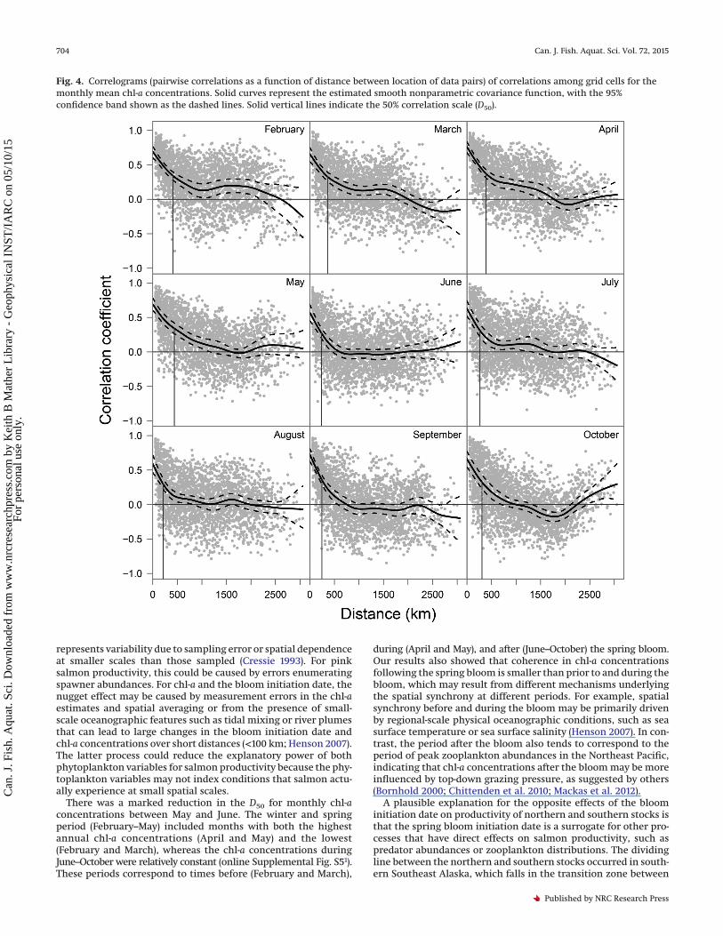
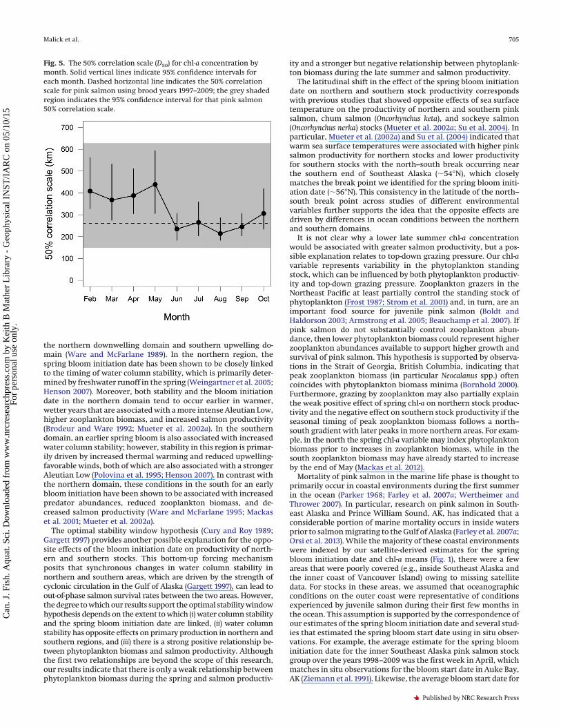
For monthly mean chl-a concentrations, covariation decayedsteeply with increasing distance over spatial scales of 0–500 kmfor all months (Fig. 4). The D50 was highest (�380 to 430 km)during the winter and spring (February–May) and declined toabout 250 km during summer and fall (June–October), which wassimilar to the estimated D50 for salmon productivity (Fig. 5). Inaddition, confidence intervals for the chl-a D50 for all monthsoverlapped the confidence intervals for salmon productivity D50

values (Fig. 5). The CZD for chl-a concentrations ranged from 0.56in June to 0.76 in April, which was slightly higher than the esti-mated CZD for the bloom initiation date and salmon productivity.

Single-stock modelsThe single-stock Ricker models indicated that pink salmon pro-

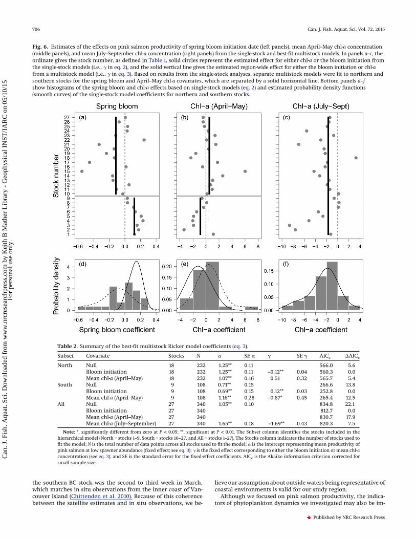
ductivity was related to the spring bloom initiation date eitherpositively (15 stocks) or negatively (12 stocks) (Fig. 6a). The distri-bution of model coefficients (i.e., � in eq. 2) ranged from −0.55 to0.25 and was asymmetric about zero, with the majority of valuesbetween −0.2 and 0.25 (Fig. 6d). Productivity of all nine pinksalmon stocks south of northern Southeast Alaska (i.e., stocks 1–9in Table 1) was positively related to the spring bloom initiationdate, whereas productivity of northern stocks was mostly nega-tively related (12 of 18 stocks; Fig. 6a). The intervention modelindicated a significant break (P < 0.05) in the sign of these rela-tionships near 55.7°N, which was between the southern SoutheastAlaska stock (stock 9) and the northern Southeast Alaska outsidestock (stock 10; Fig. 1).

Pink salmon productivity was also both positively (14 stocks)and negatively (13 stocks) related to spring chl-a concentrations(Fig. 6b), with the coefficients ranging from −3.4 to 6.0 (Fig. 6e).Like the bloom initiation date, the intervention model indicated a

Malick et al. 701

Published by NRC Research Press

Can

. J. F

ish.

Aqu

at. S

ci. D

ownl

oade

d fr

om w

ww

.nrc

rese

arch

pres

s.co

m b

y K

eith

B M

athe

r L

ibra

ry -

Geo

phys

ical

IN

ST/I

AR

C o

n 05

/10/

15Fo

r pe

rson

al u

se o

nly.

significant break (P < 0.05) between stocks 9 and 10 for the springchl-a coefficients (Fig. 6b). Productivity for all but two stocks in thesouthern group had a negative relationship with spring chl-a con-centrations, whereas the northern group had a mix of positiveand negative relationships.

For the late summer chl-a variable, productivity was consis-tently negatively related to chl-a, with only 4 of the 27 stockshaving a positive relationship (Fig. 6c). The coefficients were ap-proximately normally distributed, with the magnitudes rangingfrom −8.6 to 3.2 and a median value of −1.9 (Fig. 6f). In contrastwith the other two phytoplankton variables, the interventionmodel did not indicate a significant break in the sign of the coef-ficients between northern and southern stocks (Fig. 6c).

The productivity parameters (�) for the bloom initiation dateand both chl-a models were approximately normally distributed(a requirement for the multistock models), but the distribution ofthe density-dependent coefficients (�) had a long left tail (onlineSupplemental Fig. S31).

Multistock modelsOver all pink salmon stocks we considered, productivity was

significantly related to spring bloom initiation date (northern andsouthern models), spring chl-a concentrations (southern modelonly), and late summer chl-a concentrations (� in Table 2), al-though stock-specific differences were not significant in any mod-els. For the bloom initiation date, regional effects were opposite insign for the northern and southern stock groups (� in rows 2 and5 in Table 2; Fig. 6a), suggesting that salmon productivity for thesouthern stock group is higher than average when the bloom islater (positive coefficient), whereas productivity is higher thanaverage for the northern stock group when the bloom is early(negative coefficient). This result contrasts with those for spring(southern model only) and late summer chl-a, where the regionaleffect was negative, implying reduced salmon productivity whenchl-a concentrations are higher (� in rows 6 and 10 in Table 2).Furthermore, the spring bloom initiation date was a better pre-dictor of salmon productivity than mean chl-a concentration for

Fig. 2. Correlograms (pairwise correlations as a function of distance between location of data pairs) of correlations among salmonproductivity indices across all brood years (a), salmon productivity for brood years 1997–2009 (b), and spring bloom initiation date (c). Solidcurves represent the estimated smooth nonparametric covariance function, with 95% confidence band shown as the dashed lines. Solidvertical lines indicate the 50% correlation scale (D50).

702 Can. J. Fish. Aquat. Sci. Vol. 72, 2015

Published by NRC Research Press

Can

. J. F

ish.

Aqu

at. S

ci. D

ownl

oade

d fr

om w

ww

.nrc

rese

arch

pres

s.co

m b

y K

eith

B M

athe

r L

ibra

ry -

Geo

phys

ical

IN

ST/I

AR

C o

n 05

/10/

15Fo

r pe

rson

al u

se o

nly.

all subsets of data (i.e., northern stock group, southern stockgroup, and all stocks; AICc values in Table 2).

Estimates of the regional effect of the spring bloom initiationdate on salmon productivity were significantly different than zerofor both northern and southern multistock models (� in rows 2and 5 in Table 2), but the models were not significantly differentthan the full model (eq. 3), which included both the regional andstock-specific effects (L = 0.03, P > 0.1). The estimated region-wideeffect of spring chl-a concentrations on salmon productivity ofsouthern stocks and late summer chl-a on productivity of allstocks were significantly different from zero (� in rows 6 and 10 inTable 2). However, for both models and chl-a variables, there wasno evidence of stock-specific effects based on likelihood ratio testscomparing the full models with a model without the random chl-aeffects (L = 0.001, P > 0.1 for both spring and late summer chl-a). Inaddition, for the northern stock group there was no support foreither a regional or stock-specific effect of spring chl-a (row 3 inTable 2; L = 0.001, P > 0.1).

In both the northern and southern areas, the bloom initiationdate had a stronger effect on pink salmon productivity thanspring chl-a concentrations as shown by the AICc of 5.4 betweenthe best-fit models for chl-a and the bloom initiation for the north-ern stock group and 12.5 for the southern stock group (Table 2).The bloom initiation date also had the highest relative impor-tance (AICc = 0) when the northern and southern models werecombined with an AICc value considerable less than late summer

chl-a, spring chl-a, and the null model (rows 7–10 in Table 2).Between the two chl-a variables, the late summer chl-a mean hada higher relative importance (i.e., lower AICc value) than the meanspring chl-a concentration as indicated by the 10 unit differencebetween AICc values (rows 9 and 10 in Table 2).

Sensitivity analysisOur estimates of the spatial covariation in pink salmon produc-

tivity were not sensitive to the form of stock–recruit model be-cause residuals from the Ricker and Beverton–Holt models werehighly correlated (mean correlation across stocks = 0.97). The D50and CZD values were nearly identical between models fit using theRicker and Beverton–Holt residuals. Similarly, the spatial analyseswere not sensitive to the interpolation of data points in the chl-atime series. The difference between D50 values for the interpolatedand noninterpolated spring bloom series was 10 km, with almostcomplete overlap of the confidence intervals. In addition, changes inD50 for monthly chl-a without interpolation values ranged from 0 to10 km across months with almost complete overlap of the confi-dence intervals. Coefficients of the multistock Ricker model werealso insensitive to the interpolation of missing data.

The results from the multistock models were not sensitive toour initial assumption of uncorrelated errors. Specifically, thesingle-stock models did not indicate strongly autocorrelated er-rors, and adding an autocorrelated error term to the best-fit mul-tistock models did not substantially improve the fits for any of themodels, which is consistent with other research on pink salmonproductivity (Pyper et al. 2001). In addition, comparisons betweenthe three chl-a metrics and hatchery marine survival rates broadlyagreed with the results of the multistock models (online Supple-mental data B and Fig. S41).

DiscussionWe investigated two indices of phytoplankton dynamics, spring

bloom initiation date and mean chl-a concentration, to betterunderstand the potential mechanisms linking biological oceano-graphic conditions to Pacific salmon productivity. Our results in-dicated that (i) spatial covariation patterns for the spring bloominitiation date, mean chl-a concentration, and pink salmon pro-ductivity were similar, with strongest positive covariation at theregional scale (0–800 km); (ii) there were opposing effects of thespring bloom initiation date on northern and southern pinksalmon stock productivity, with an early bloom initiation datebeing associated with higher northern stock productivity and alate bloom being associated with higher southern stock produc-tivity; (iii) phytoplankton biomass during the late summer (July–September) was more strongly associated with salmon productivitythan phytoplankton biomass during the spring (April–May); and(iv) the spring bloom initiation date was a better predictor ofsalmon productivity than mean chl-a concentration for bothsouthern and northern stocks.

Spatial synchrony for all three variables was strongest at re-gional spatial scales and declined rapidly with increasing dis-tance. For the bloom initiation date and chl-a concentration, thissuggests that physical processes operating on relatively small spa-tial scales (e.g., summer sea surface temperature and sea surfacesalinity) drives the spatial variability, rather than larger-scale at-mospheric processes such as the Pacific Decadal Oscillation (Mueteret al. 2002b). For pink salmon productivity, our results suggestthat both phytoplankton biomass and the bloom initiation datecould be factors driving the regional-scale covariation. Further-more, the match in spatial synchrony between both phytoplank-ton variables and salmon productivity supports the inclusion ofthese variables in the single-stock and multistock models and alsolends support for the observed correlations between pink salmonproductivity and both phytoplankton variables.

Spatial correlation of all three variables was less than one atzero distance, indicating the presence of a “nugget effect”, which

Fig. 3. Comparison of the estimated 50% correlation scale (D50;panel a) and y intercept (CZD; panel b) for the nonparametriccovariance functions fit to pink salmon residuals using all broodyears of data (“Pink all” from Fig. 2a), pink salmon residuals usingonly brood years 1997–2009 (“Pink short” from Fig. 2b), andinitiation date for the spring bloom (from Fig. 2c). Dots indicatepoint estimates for each metric and vertical lines give 95%confidence intervals.

Malick et al. 703

Published by NRC Research Press

Can

. J. F

ish.

Aqu

at. S

ci. D

ownl

oade

d fr

om w

ww

.nrc

rese

arch

pres

s.co

m b

y K

eith

B M

athe

r L

ibra

ry -

Geo

phys

ical

IN

ST/I

AR

C o

n 05

/10/

15Fo

r pe

rson

al u

se o

nly.

represents variability due to sampling error or spatial dependenceat smaller scales than those sampled (Cressie 1993). For pinksalmon productivity, this could be caused by errors enumeratingspawner abundances. For chl-a and the bloom initiation date, thenugget effect may be caused by measurement errors in the chl-aestimates and spatial averaging or from the presence of small-scale oceanographic features such as tidal mixing or river plumesthat can lead to large changes in the bloom initiation date andchl-a concentrations over short distances (<100 km; Henson 2007).The latter process could reduce the explanatory power of bothphytoplankton variables for salmon productivity because the phy-toplankton variables may not index conditions that salmon actu-ally experience at small spatial scales.

There was a marked reduction in the D50 for monthly chl-aconcentrations between May and June. The winter and springperiod (February–May) included months with both the highestannual chl-a concentrations (April and May) and the lowest(February and March), whereas the chl-a concentrations duringJune–October were relatively constant (online Supplemental Fig. S51).These periods correspond to times before (February and March),

during (April and May), and after (June–October) the spring bloom.Our results also showed that coherence in chl-a concentrationsfollowing the spring bloom is smaller than prior to and during thebloom, which may result from different mechanisms underlyingthe spatial synchrony at different periods. For example, spatialsynchrony before and during the bloom may be primarily drivenby regional-scale physical oceanographic conditions, such as seasurface temperature or sea surface salinity (Henson 2007). In con-trast, the period after the bloom also tends to correspond to theperiod of peak zooplankton abundances in the Northeast Pacific,indicating that chl-a concentrations after the bloom may be moreinfluenced by top-down grazing pressure, as suggested by others(Bornhold 2000; Chittenden et al. 2010; Mackas et al. 2012).

A plausible explanation for the opposite effects of the bloominitiation date on productivity of northern and southern stocks isthat the spring bloom initiation date is a surrogate for other pro-cesses that have direct effects on salmon productivity, such aspredator abundances or zooplankton distributions. The dividingline between the northern and southern stocks occurred in south-ern Southeast Alaska, which falls in the transition zone between

Fig. 4. Correlograms (pairwise correlations as a function of distance between location of data pairs) of correlations among grid cells for themonthly mean chl-a concentrations. Solid curves represent the estimated smooth nonparametric covariance function, with the 95%confidence band shown as the dashed lines. Solid vertical lines indicate the 50% correlation scale (D50).

704 Can. J. Fish. Aquat. Sci. Vol. 72, 2015

Published by NRC Research Press

Can

. J. F

ish.

Aqu

at. S

ci. D

ownl

oade

d fr

om w

ww

.nrc

rese

arch

pres

s.co

m b

y K

eith

B M

athe

r L

ibra

ry -

Geo

phys

ical

IN

ST/I

AR

C o

n 05

/10/

15Fo

r pe

rson

al u

se o

nly.

the northern downwelling domain and southern upwelling do-main (Ware and McFarlane 1989). In the northern region, thespring bloom initiation date has been shown to be closely linkedto the timing of water column stability, which is primarily deter-mined by freshwater runoff in the spring (Weingartner et al. 2005;Henson 2007). Moreover, both stability and the bloom initiationdate in the northern domain tend to occur earlier in warmer,wetter years that are associated with a more intense Aleutian Low,higher zooplankton biomass, and increased salmon productivity(Brodeur and Ware 1992; Mueter et al. 2002a). In the southerndomain, an earlier spring bloom is also associated with increasedwater column stability; however, stability in this region is primar-ily driven by increased thermal warming and reduced upwelling-favorable winds, both of which are also associated with a strongerAleutian Low (Polovina et al. 1995; Henson 2007). In contrast withthe northern domain, these conditions in the south for an earlybloom initiation have been shown to be associated with increasedpredator abundances, reduced zooplankton biomass, and de-creased salmon productivity (Ware and McFarlane 1995; Mackaset al. 2001; Mueter et al. 2002a).

The optimal stability window hypothesis (Cury and Roy 1989;Gargett 1997) provides another possible explanation for the oppo-site effects of the bloom initiation date on productivity of north-ern and southern stocks. This bottom-up forcing mechanismposits that synchronous changes in water column stability innorthern and southern areas, which are driven by the strength ofcyclonic circulation in the Gulf of Alaska (Gargett 1997), can lead toout-of-phase salmon survival rates between the two areas. However,the degree to which our results support the optimal stability windowhypothesis depends on the extent to which (i) water column stabilityand the spring bloom initiation date are linked, (ii) water columnstability has opposite effects on primary production in northern andsouthern regions, and (iii) there is a strong positive relationship be-tween phytoplankton biomass and salmon productivity. Althoughthe first two relationships are beyond the scope of this research,our results indicate that there is only a weak relationship betweenphytoplankton biomass during the spring and salmon productiv-

ity and a stronger but negative relationship between phytoplank-ton biomass during the late summer and salmon productivity.

The latitudinal shift in the effect of the spring bloom initiationdate on northern and southern stock productivity correspondswith previous studies that showed opposite effects of sea surfacetemperature on the productivity of northern and southern pinksalmon, chum salmon (Oncorhynchus keta), and sockeye salmon(Oncorhynchus nerka) stocks (Mueter et al. 2002a; Su et al. 2004). Inparticular, Mueter et al. (2002a) and Su et al. (2004) indicated thatwarm sea surface temperatures were associated with higher pinksalmon productivity for northern stocks and lower productivityfor southern stocks with the north–south break occurring nearthe southern end of Southeast Alaska (�54°N), which closelymatches the break point we identified for the spring bloom initi-ation date (�56°N). This consistency in the latitude of the north–south break point across studies of different environmentalvariables further supports the idea that the opposite effects aredriven by differences in ocean conditions between the northernand southern domains.

It is not clear why a lower late summer chl-a concentrationwould be associated with greater salmon productivity, but a pos-sible explanation relates to top-down grazing pressure. Our chl-avariable represents variability in the phytoplankton standingstock, which can be influenced by both phytoplankton productiv-ity and top-down grazing pressure. Zooplankton grazers in theNortheast Pacific at least partially control the standing stock ofphytoplankton (Frost 1987; Strom et al. 2001) and, in turn, are animportant food source for juvenile pink salmon (Boldt andHaldorson 2003; Armstrong et al. 2005; Beauchamp et al. 2007). Ifpink salmon do not substantially control zooplankton abun-dance, then lower phytoplankton biomass could represent higherzooplankton abundances available to support higher growth andsurvival of pink salmon. This hypothesis is supported by observa-tions in the Strait of Georgia, British Columbia, indicating thatpeak zooplankton biomass (in particular Neocalanus spp.) oftencoincides with phytoplankton biomass minima (Bornhold 2000).Furthermore, grazing by zooplankton may also partially explainthe weak positive effect of spring chl-a on northern stock produc-tivity and the negative effect on southern stock productivity if theseasonal timing of peak zooplankton biomass follows a north–south gradient with later peaks in more northern areas. For exam-ple, in the north the spring chl-a variable may index phytoplanktonbiomass prior to increases in zooplankton biomass, while in thesouth zooplankton biomass may have already started to increaseby the end of May (Mackas et al. 2012).

Mortality of pink salmon in the marine life phase is thought toprimarily occur in coastal environments during the first summerin the ocean (Parker 1968; Farley et al. 2007a; Wertheimer andThrower 2007). In particular, research on pink salmon in South-east Alaska and Prince William Sound, AK, has indicated that aconsiderable portion of marine mortality occurs in inside watersprior to salmon migrating to the Gulf of Alaska (Farley et al. 2007a;Orsi et al. 2013). While the majority of these coastal environmentswere indexed by our satellite-derived estimates for the springbloom initiation date and chl-a means (Fig. 1), there were a fewareas that were poorly covered (e.g., inside Southeast Alaska andthe inner coast of Vancouver Island) owing to missing satellitedata. For stocks in these areas, we assumed that oceanographicconditions on the outer coast were representative of conditionsexperienced by juvenile salmon during their first few months inthe ocean. This assumption is supported by the correspondence ofour estimates of the spring bloom initiation date and several stud-ies that estimated the spring bloom start date using in situ obser-vations. For example, the average estimate for the spring bloominitiation date for the inner Southeast Alaska pink salmon stockgroup over the years 1998–2009 was the first week in April, whichmatches in situ observations for the bloom start date in Auke Bay,AK (Ziemann et al. 1991). Likewise, the average bloom start date for

Fig. 5. The 50% correlation scale (D50) for chl-a concentration bymonth. Solid vertical lines indicate 95% confidence intervals foreach month. Dashed horizontal line indicates the 50% correlationscale for pink salmon using brood years 1997–2009; the grey shadedregion indicates the 95% confidence interval for that pink salmon50% correlation scale.

Malick et al. 705

Published by NRC Research Press

Can

. J. F

ish.

Aqu

at. S

ci. D

ownl

oade

d fr

om w

ww

.nrc

rese

arch

pres

s.co

m b

y K

eith

B M

athe

r L

ibra

ry -

Geo

phys

ical

IN

ST/I

AR

C o

n 05

/10/

15Fo

r pe

rson

al u

se o

nly.

the southern BC stock was the second to third week in March,which matches in situ observations from the inner coast of Van-couver Island (Chittenden et al. 2010). Because of this coherencebetween the satellite estimates and in situ observations, we be-

lieve our assumption about outside waters being representative ofcoastal environments is valid for our study region.

Although we focused on pink salmon productivity, the indica-tors of phytoplankton dynamics we investigated may also be im-

Fig. 6. Estimates of the effects on pink salmon productivity of spring bloom initiation date (left panels), mean April–May chl-a concentration(middle panels), and mean July–September chl-a concentration (right panels) from the single-stock and best-fit multistock models. In panels a–c, theordinate gives the stock number, as defined in Table 1, solid circles represent the estimated effect for either chl-a or the bloom initiation fromthe single-stock models (i.e., � in eq. 2), and the solid vertical line gives the estimated region-wide effect for either the bloom initiation or chl-afrom a multistock model (i.e., � in eq. 3). Based on results from the single-stock analyses, separate multistock models were fit to northern andsouthern stocks for the spring bloom and April–May chl-a covariates, which are separated by a solid horizontal line. Bottom panels d–fshow histograms of the spring bloom and chl-a effects based on single-stock models (eq. 2) and estimated probability density functions(smooth curves) of the single-stock model coefficients for northern and southern stocks.

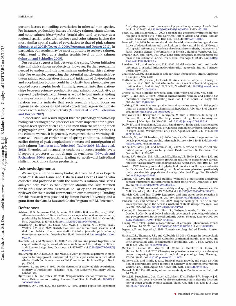
Table 2. Summary of the best-fit multistock Ricker model coefficients (eq. 3).

Subset Covariate Stocks N � SE � � SE � AICc AICc

North Null 18 232 1.25** 0.11 566.0 5.6Bloom initiation 18 232 1.25** 0.11 −0.12** 0.04 560.3 0.0Mean chl-a (April–May) 18 232 1.07** 0.16 0.51 0.32 565.7 5.4

South Null 9 108 0.71** 0.15 266.6 13.8Bloom initiation 9 108 0.69** 0.15 0.12** 0.03 252.8 0.0Mean chl-a (April–May) 9 108 1.16** 0.28 −0.87* 0.45 265.4 12.5

All Null 27 340 1.05** 0.10 834.8 22.1Bloom initiation 27 340 812.7 0.0Mean chl-a (April–May) 27 340 830.7 17.9Mean chl-a (July–September) 27 340 1.65** 0.18 −1.69** 0.43 820.3 7.5

Note: *, significantly different from zero at P < 0.05; **, significant at P < 0.01. The Subset column identifies the stocks included in thehierarchical model (North = stocks 1–9, South = stocks 10–27, and All = stocks 1–27). The Stocks column indicates the number of stocks used tofit the model; N is the total number of data points across all stocks used to fit the model; � is the intercept representing mean productivity ofpink salmon at low spawner abundance (fixed effect; see eq. 3); � is the fixed effect corresponding to either the bloom initiation or mean chl-aconcentration (see eq. 3); and SE is the standard error for the fixed-effect coefficients. AICc is the Akaike information criterion corrected forsmall sample size.

706 Can. J. Fish. Aquat. Sci. Vol. 72, 2015

Published by NRC Research Press

Can

. J. F

ish.

Aqu

at. S

ci. D

ownl

oade

d fr

om w

ww

.nrc

rese

arch

pres

s.co

m b

y K

eith

B M

athe

r L

ibra

ry -

Geo

phys

ical

IN

ST/I

AR

C o

n 05

/10/

15Fo

r pe

rson

al u

se o

nly.

portant factors controlling covariation in other salmon species.For instance, productivity indices of sockeye salmon, chum salmon,and coho salmon (Oncorhynchus kisutch) also tend to covary at aregional spatial scale, with sockeye and coho salmon having themost similar spatial scales of covariation to that of pink salmon(Mueter et al. 2002b; Teo et al. 2009; Peterman and Dorner 2012). Inparticular, our results may be most applicable to sockeye salmon,which tend to feed at a similar trophic level as pink salmon(Johnson and Schindler 2009).

Our results suggest a link between the spring bloom initiationdate and pink salmon productivity; however, further research isneeded to understand the mechanisms underlying this relation-ship. For example, comparing the potential match–mismatch be-tween salmon out-migration timing and initiation of phytoplanktonand zooplankton blooms could help clarify how phenologies arecoupled across trophic levels. Similarly, research into the relation-ships between primary productivity and salmon productivity, asopposed to phytoplankton biomass, would help in understandingthe importance of the optimal stability window. Our spatial cor-relation results indicate that such research should focus onregional-scale processes and avoid correlating large-scale climateindices with salmon productivity (Mueter et al. 2002a; Petermanand Dorner 2012).

In conclusion, our results suggest that the phenology of bottom-upbiological oceanographic processes are more important for higher-trophic-level species such as pink salmon than the standing stockof phytoplankton. This conclusion has important implications asthe climate warms. It is generally recognized that a warming cli-mate will lead to an earlier onset of spring conditions, includingearlier timing of peak zooplankton biomass and outmigration ofpink salmon (Parmesan and Yohe 2003; Taylor 2008; Mackas et al.2012). Phenological mismatches could occur across trophic levelsif separate processes do not change in synchrony (Edwards andRichardson 2004), potentially leading to northward latitudinalshifts in peak pink salmon productivity.

AcknowledgementsWe are grateful to the many biologists from the Alaska Depart-

ment of Fish and Game and Fisheries and Oceans Canada whocollected and provided us with the numerous salmon time seriesanalyzed here. We also thank Nathan Mantua and Todd Mitchellfor helpful discussions, as well as Ed Farley and an anonymousreviewer for their useful comments on our manuscript. Fundingfor this research was provided by Simon Fraser University and agrant from the Canada Research Chairs Program to R.M. Peterman.

ReferencesAdkison, M.D., Peterman, R.M., Lapointe, M.F., Gillis, D.M., and Korman, J. 1996.

Alternative models of climatic effects on sockeye salmon, Oncorhynchus nerka,productivity in Bristol Bay, Alaska, and the Fraser River, British Columbia.Fish. Oceanogr. 5: 137–152. doi:10.1111/j.1365-2419.1996.tb00113.x.

Armstrong, J.L., Boldt, J.L., Cross, A.D., Moss, J.H., Davis, N.D., Myers, K.W.,Walker, R.V., et al. 2005. Distribution, size, and interannual, seasonal anddiel food habits of northern Gulf of Alaska juvenile pink salmon,Oncorhynchus gorbuscha. Deep-Sea Res. II, 52: 247–265. doi:10.1016/j.dsr2.2004.09.019.

Beamish, R.J., and Mahnken, C. 2001. A critical size and period hypothesis toexplain natural regulation of salmon abundance and the linkage to climateand climate change. Prog. Oceanogr. 49: 423–437. doi:10.1016/S0079-6611(01)00034-9.

Beauchamp, D.A., Cross, A.D., and Moss, J.H. 2007. Interannual patterns in stage-specific feeding, growth, and survival of juvenile pink salmon in the Gulf ofAlaska. North Pacific Anadromous Fish Commission, Technical Report No. 7.pp. 35–36.

Beverton, R., and Holt, S. 1957. On the dynamics of exploited fish populations.Ministry of Agriculture, Fisheries; Food, Her Majesty’s Stationary Office,London, UK.

Bjørnstad, O.N., and Falck, W. 2001. Nonparametric spatial covariance func-tions: Estimation and testing. Environ. Ecol. Stat. 8: 53–70. doi:10.1023/A:1009601932481.

Bjørnstad, O.N., Ims, R.A., and Lambin, X. 1999. Spatial population dynamics:

Analyzing patterns and processes of population synchrony. Trends Ecol.Evol. 14: 427–432. doi:10.1016/S0169-5347(99)01677-8. PMID:10511718.

Boldt, J.L., and Haldorson, L.J. 2003. Seasonal and geographic variation in juve-nile pink salmon diets in the Northern Gulf of Alaska and Prince WilliamSound. Trans. Am. Fish. Soc. 132: 1035–1052. doi:10.1577/T02-091.

Bornhold, E.A. 2000. Interannual and interdecadal patterns in timing and abun-dance of phytoplankton and zooplankton in the central Strait of Georgia,with special reference to Neocalanus plumchrus. Master’s thesis, Department ofEarth, Ocean Sciences, The University of British Columbia, Vancouver, B.C.

Brodeur, R.D., and Ware, D.M. 1992. Long-term variability in zooplankton bio-mass in the subarctic Pacific Ocean. Fish. Oceanogr. 1: 32–38. doi:10.1111/j.1365-2419.1992.tb00023.x.

Burnham, K.P., and Anderson, D.R. 2002. Model selection and multimodelinference: a practical information-theoretical approach. 2nd ed. Springer-Verlag, New York.

Chatfield, C. 2004. The analysis of time series: an introduction. 6th ed. Chapman& Hall/CRC, New York.

Chittenden, C.M., Jensen, J.L., Ewart, D., Anderson, S., Balfry, S., Downey, E.,Eaves, A., et al. 2010. Recent salmon declines: a result of lost feeding oppor-tunities due to bad timing? PloS ONE, 5: e12423. doi:10.1371/journal.pone.0012423. PMID:20805978.

Cressie, N. 1993. Statistics for spatial data. John Wiley and Sons, New York.Cury, P., and Roy, C. 1989. Optimal environmental window and pelagic fish

recruitment success in upwelling areas. Can. J. Fish. Aquat. Sci. 46(4): 670–680. doi:10.1139/f89-086.

Cushing, D.H. 1990. Plankton production and year-class strength in fish popula-tions: an update of the match/mismatch hypothesis. Adv. Mar. Biol. 26: 249–293. doi:10.1016/S0065-2881(08)60202-3.

Drinkwater, K.F., Beaugrand, G., Kaeriyama, M., Kim, S., Ottersen, G., Perry, R.I.,Pörtner, H.O., et al. 2010. On the processes linking climate to ecosystemchanges. J. Mar. Syst. 79: 374–388. doi:10.1016/j.jmarsys.2008.12.014.

Duffy, E.J., and Beauchamp, D.A. 2011. Rapid growth in the early marine periodimproves the marine survival of Chinook salmon (Oncorhynchus tshawytscha)in Puget Sound, Washington. Can. J. Fish. Aquat. Sci. 68(2): 232–240. doi:10.1139/F10-144.

Edwards, M., and Richardson, A.J. 2004. Impact of climate change on marinepelagic phenology and trophic mismatch. Nature, 430: 881–884. doi:10.1038/nature02808. PMID:15318219.

Farley, E.V., Moss, J.H., and Beamish, R.J. 2007a. A review of the critical size,critical period hypothesis for juvenile Pacific salmon. N. Pac. Anad. FishComm. Bull. 4: 311–317.

Farley, E.V., Murphy, J.M., Adkison, M.D., Eisner, L.B., Helle, J.H., Moss, J.H., andNielsen, J. 2007b. Early marine growth in relation to marine-stage survivalrates for Alaska sockeye salmon (Oncorhynchus nerka). Fish. Bull. 105: 121–130.

Frost, B. 1987. Grazing control of phytoplankton stock in the open subarcticPacific Ocean: A model assessing the role of mesozooplankton, particularlythe large calanoid copepods Neocalanus spp. Mar. Ecol. Progr. Ser. 39: 49–68.doi:10.3354/meps039049.

Gargett, A.E. 1997. The optimal stability “window”: a mechanism underlyingdecadal fluctuations in North Pacific salmon stocks? Fish. Oceanogr. 6: 109–117. doi:10.1046/j.1365-2419.1997.00033.x.

Henson, S.A. 2007. Water column stability and spring bloom dynamics in theGulf of Alaska. J. Mar. Res. 65: 715–736. doi:10.1357/002224007784219002.

Hurvich, C.M., and Tsai, C. 1989. Regression and time series model selection insmall samples. Biometrika, 76: 297–307. doi:10.1093/biomet/76.2.297.

Johnson, S.P., and Schindler, D.E. 2009. Trophic ecology of Pacific salmon(Oncorhynchus spp.) in the ocean: a synthesis of stable isotope research. Ecol.Res. 24: 855–863. doi:10.1007/s11284-008-0559-0.

Koeller, P., Fuentes-Yaco, C., Platt, T., Sathyendranath, S., Richards, A.,Ouellet, P., Orr, D., et al. 2009. Basin-scale coherence in phenology of shrimpsand phytoplankton in the North Atlantic Ocean. Science, 324: 791–793. doi:10.1126/science.1170987. PMID:19423827.

Koenig, W.D. 1999. Spatial autocorrelation of ecological phenomena. TrendsEcol. Evol. 14: 22–26. doi:10.1016/S0169-5347(98)01533-X. PMID:10234243.

Legendre, P., and Legendre, L. 1998. Numerical ecology. 2nd ed. Elsevier, Amster-dam.

Mackas, D.L., Thomson, R.E., and Galbraith, M. 2001. Changes in the zooplank-ton community of the British Columbia continental margin, 1985–1999, andtheir covariation with oceanographic conditions. Can. J. Fish. Aquat. Sci.58(4): 685–702. doi:10.1139/f01-009.

Mackas, D., Greve, W., Edwards, M., Chiba, S., Tadokoro, K., Eloire, D.,Mazzocchi, M., et al. 2012. Changing zooplankton seasonality in a changingocean: comparing time series of zooplankton phenology. Prog. Oceanogr.97-100: 31–62. doi:10.1016/j.pocean.2011.11.005.

Mathews, S.B., and Ishida, Y. 1989. Survival, ocean growth, and ocean distribu-tion of differentially timed releases of hatchery coho salmon (Oncorhynchuskisutch). Can. J. Fish. Aquat. Sci. 46(7): 1216–1226. doi:10.1139/f89-157.

McGurk, M.D. 1996. Allometry of marine mortality of Pacific salmon. Fish. Bull.94: 77–88.

Moss, J.H., Beauchamp, D.A., Cross, A.D., Myers, K.W., Farley, E.V., Murphy, J.M.,and Helle, J.H. 2005. Evidence for size-selective mortality after the first sum-mer of ocean growth by pink salmon. Trans. Am. Fish. Soc. 134: 1313–1322.doi:10.1577/T05-054.1.

Malick et al. 707

Published by NRC Research Press

Can

. J. F

ish.

Aqu

at. S

ci. D

ownl

oade

d fr

om w

ww

.nrc

rese

arch

pres

s.co

m b

y K

eith

B M

athe

r L

ibra

ry -

Geo

phys

ical

IN

ST/I

AR

C o

n 05

/10/

15Fo

r pe

rson

al u

se o

nly.

Mueter, F.J., Peterman, R.M., and Pyper, B.J. 2002a. Opposite effects of oceantemperature on survival rates of 120 stocks of Pacific salmon (Oncorhynchus spp.)in northern and southern areas. Can. J. Fish. Aquat. Sci. 59(3): 456–463.[Corrigendum printed in Can. J. Fish. Aquat. Sci. 60(6): 757.] doi:10.1139/f02-020.

Mueter, F.J., Ware, D.M., and Peterman, R.M. 2002b. Spatial correlation patternsin coastal environmental variables and survival rates of salmon in the north-east Pacific Ocean. Fish. Oceanogr. 11: 205–218. doi:10.1046/j.1365-2419.2002.00192.x.

Myers, R.A., and Mertz, G. 1998. Reducing uncertainty in the biological basis offisheries management by meta-analysis of data from many populations: asynthesis. Fish. Res. 37: 51–60. doi:10.1016/S0165-7836(98)00126-X.

Myers, R.A., Bowen, K.G., and Barrowman, N.J. 1999. Maximum reproductive rateof fish at low population sizes. Can. J. Fish. Aquat. Sci. 56(12): 2404–2419.doi:10.1139/f99-201.

Orsi, J.A., Sturdevant, M.V., Fergusson, E.A., Heinl, S.C., Vulstek, S.C., Maselko,J.M., and Joyce, J.E. 2013. Connecting the “dots” among coastal ocean metricsand Pacific salmon production in southeast Alaska, 1997–2012. North PacificAnadromous Fish Commission Technical Report No. 9. pp. 260–266.

Ottersen, G., Kim, S., Huse, G., Polovina, J.J., and Stenseth, N.C. 2010. Majorpathways by which climate may force marine fish populations. J. Mar. Syst.79: 343–360. doi:10.1016/j.jmarsys.2008.12.013.

Parker, R.R. 1968. Marine mortality schedules of pink salmon of the Bella CoolaRiver, central British Columbia. J. Fish. Res. Board Can. 25(4): 757–794. doi:10.1139/f68-068.

Parmesan, C., and Yohe, G. 2003. A globally coherent fingerprint of climatechange impacts across natural systems. Nature, 421: 37–42. doi:10.1038/nature01286. PMID:12511946.

Peterman, R.M. 1985. Patterns of interannual variation in age at maturity ofsockeye salmon (Oncorhynchus nerka) in Alaska and British Columbia. Can. J.Fish. Aquat. Sci. 42(10): 1595–1607. doi:10.1139/f85-200.

Peterman, R., and Dorner, B. 2012. A widespread decrease in productivity ofsockeye salmon (Oncorhynchus nerka) populations in western North America.Can. J. Fish. Aquat. Sci. 69(8): 1255–1260. doi:10.1139/f2012-063.

Pinheiro, J.C., and Bates, D.M. 2000. Mixed-effects models in S and S-Plus. Statis-tics and computing. Springer Verlag, New York.

Piston, A.W., and Heinl, S.C. 2011. Pink salmon stock status and escapementgoals in Southeast Alaska. Alaska Department of Fish and Game, SpecialPublication No. 11–18.

Platt, T., Fuentes-Yaco, C., and Frank, K.T. 2003. Spring algal bloom and larvalfish survival. Nature, 423: 398–399. doi:10.1038/423398b. PMID:12761538.

Polovina, J.J., Mitchum, G.T., and Evans, G.T. 1995. Decadal and basin-scale vari-ation in mixed layer depth and the impact on biological production in theCentral and North Pacific, 1960–88. Deep-Sea Res. I Oceanogr. Res. Pap. 42:1701–1716. doi:10.1016/0967-0637(95)00075-H.

Pyper, B.J., Mueter, F.J., Peterman, R.M., Blackbourn, D.J., and Wood, C.C. 2001.Spatial covariation in survival rates of Northeast Pacific pink salmon(Oncorhynchus gorbuscha). Can. J. Fish. Aquat. Sci. 58(8): 1501–1515. doi:10.1139/f01-096.

Pyper, B.J., Mueter, F.J., and Peterman, R.M. 2005. Across-species comparisons of

spatial scales of environmental effects on survival rates of Northeast Pacificsalmon. Trans. Am. Fish. Soc. 134: 86–104. doi:10.1577/T04-034.1.

Ricker, W.E. 1954. Stock and recruitment. J. Fish. Res. Board Can. 11(5): 559–623.doi:10.1139/f54-039.

Siegel, D.A., Doney, S.C., and Yoder, J.A. 2002. The North Atlantic spring phyto-plankton bloom and Sverdrup’s critical depth hypothesis. Science, 296: 730–733. doi:10.1126/science.1069174. PMID:11976453.

Strom, S., Brainard, M., Holmes, J., and Olson, M. 2001. Phytoplankton bloomsare strongly impacted by microzooplankton grazing in coastal North Pacificwaters. Mar. Biol. 138: 355–368. doi:10.1007/s002270000461.

Su, Z., Peterman, R.M., and Haeseker, S.L. 2004. Spatial hierarchical Bayesianmodels for stock-recruitment analysis of pink salmon (Oncorhynchus gorbuscha).Can. J. Fish. Aquat. Sci. 61(12): 2471–2486. doi:10.1139/f04-168.

Sverdrup, H.U. 1953. On conditions for the vernal blooming of phytoplankton.J. Cons. Int. Explor. Mer, 18: 287–295. doi:10.1093/icesjms/18.3.287.

Taylor, S.G. 2008. Climate warming causes phenological shift in pink salmon,Oncorhynchus gorbuscha, behavior at Auke Creek, Alaska. Glob. Change Biol.14: 229–235. doi:10.1111/j.1365-2486.2007.01494.x.

Teo, S.L.H., Botsford, L.W., and Hastings, A. 2009. Spatio-temporal covariabilityin coho salmon (Oncorhynchus kisutch) survival, from California to southeastAlaska. Deep-Sea Res. II Top. Stud. Oceanogr. 56: 2570–2578. doi:10.1016/j.dsr2.2009.03.007.

Waite, J., and Mueter, F.J. 2013. Spatial and temporal variability of chlorophyll-aconcentrations in the coastal Gulf of Alaska, 1998–2011, using cloud-freereconstructions of SeaWiFS and MODIS-Aqua data. Prog. Oceanogr. 116: 179–192. doi:10.1016/j.pocean.2013.07.006.

Ware, D.M., and McFarlane, G.A. 1989. Fisheries production domains in theNortheast Pacific Ocean. In Effects of ocean variability on recruitment andan evaluation of parameters used in stock assessment models. Edited byR.J. Beamish and G.A. McFarlane. Canadian Special Publication of Fisher-ies and Aquatic Sciences 108. pp. 359–379.

Ware, D.M., and McFarlane, G.A. 1995. Climate-induced changes in Pacific hake(Merluccius productus) abundance and pelagic community interactions in theVancouver Island system. In Climate change and northern fish population.Canadian Special Publication of Fisheries and Aquatic Sciences 121. pp. 509–121.

Ware, D.M., and Thomson, R.E. 1991. Link between long-term variability in up-welling and fish production in the Northeast Pacific Ocean. Can. J. Fish.Aquat. Sci. 48(12): 2296–2306. doi:10.1139/f91-270.

Ware, D.M., and Thomson, R.E. 2005. Bottom-up ecosystem trophic dynamicsdetermine fish production in the Northeast Pacific. Science, 308: 1280–1284.doi:10.1126/science.1109049. PMID:15845876.

Weingartner, T.J., Danielson, S.L., and Royer, T.C. 2005. Freshwater variabilityand predictability in the Alaska Coastal Current. Deep-Sea Res. II Top. Stud.Oceanogr. 52: 169–191. doi:10.1016/j.dsr2.2004.09.030.

Wertheimer, A.C., and Thrower, F.P. 2007. Mortality rates of chum salmon dur-ing their early marine residency. In Ecology of juvenile salmon in the north-east Pacific Ocean: regional comparisons. Edited by C.B. Grimes, R.D. Brodeur,L.J. Haldorson, and S.M. McKinnell. American Fisheries Society, Symposium57, Bethesda, Md. pp. 233–247.

Ziemann, D., Conquest, L., Olaizola, M., and Bienfang, P. 1991. Interannual vari-ability in the spring phytoplankton bloom in Auke Bay, Alaska. Mar. Biol.109: 321–334. doi:10.1007/BF01319400.

708 Can. J. Fish. Aquat. Sci. Vol. 72, 2015

Published by NRC Research Press

Can

. J. F

ish.

Aqu

at. S

ci. D

ownl

oade

d fr

om w

ww

.nrc

rese

arch

pres

s.co

m b

y K

eith

B M

athe

r L

ibra

ry -

Geo

phys

ical

IN

ST/I

AR

C o

n 05

/10/

15Fo

r pe

rson

al u

se o

nly.