implementation of an ldpc decoder for the dvb-s2, -t2 and -c2 standards
TRANSCRIPT

Implementation of an LDPC decoder for the
DVB-S2, -T2 and -C2 standards
Cedric Marchand
30/11/2010


”If we knew what it was we were doing, it would not be called research,would it?”
Albert Einstein (1879-1955)
i

Remerciements
Je tiens tout d’abord a remercier Emmanuel Boutillon pour m’avoir en-cadre avec serieux et clairvoyance. Je remercie aussi Laura Conde-Canenciapour son aide lors de la redaction des differents articles et de la these.
Je remercie tous mes encadrants qui se sont succedes dans un contexte deplan social et de restructuration NXP: Patrick Lecluse initiateur de la theseCIFFRE, Jean-Baptiste DORE qui m’a ete d’une grande aide en debut dethese, puis Pascal Frederic et enfin Didier Lohy.
Je remercie mes collegues de travail au sein du group NXP: Arnaud,Pierre-Jean, Zair, Carol et Franck.
Je n’oublie pas mes collegues a l’Univerite de Bretagne Sud dont Sebastien,Antoine et Jeremie qui finissaient leur these et dont j’ai pu beneficier desconseils avises; Gizlaine et Rachid, collegues de promotion et amis qui ontcommences leur Master recherche et leur these en meme temps que moi;Gorgiano mon voisin d’en face; Aswhani et sa bonne humeur, le personneladministratif et le personnel du restaurant universitaire.
Enfin, je remercie ma famille pour son soutient et Monika pour son sup-port quotidien et ses bons petits plats.
ii

Resume
Les codes correcteurs d’erreurs LDPC (“Low Density Parity Check” oumatrice de parite a faible densite) font partie des codes en bloc permettantde s’approcher a quelques dixieme de dB de la limite de Shannon. Ces re-marquables performances associees a leur relative simplicite de decodage ren-dent ces codes tres attractifs pour les systemes de transmissions numeriques.C’est notamment le cas pour la norme de telediffusion numerique par satel-lite (DVB-S2) et la norme de telediffusion numerique terrestre (DVB-T2) quiutilisent un code LDPC irregulier pour la protection de la transmission desdonnees. Cette these porte sur l’optimisation de l’implementation materielled’un decodeur LDPC pour les standards DVB-S2, -T2 et -C2. Apres uneetude de l’etat de l’art, c’est le decodeur par couche (layered decoder) qui aete choisi comme architecture de base a l’implementation du decodeur. Nousnous sommes ensuite confrontes au probleme des conflits memoires inherentsa la structure particuliere des standards DVB-S2, -T2 et -C2. Deux nouvellescontributions ont ete apportees a la resolution de ce probleme. Une baseesur la constitution d’une matrice equivalente et l’autre basee sur la repetitionde couches (layers). Les conflits memoire dues au pipeline sont quant a euxsuprimes a l’aide d’un ordonnancement des layers et des matrices identites.L’espace memoire etant un differenciateur majeur de cout d’implementation,la reduction au minimum de la taille memoire a ete etudiee. Une saturationoptimisee et un partitionnement optimal des bancs memoires ont permisune reduction significative de l’espace memoire par rapport a l’etat de l’art.De plus, l’utilisation de RAM simple port a la place de RAM double portest aussi propose pour reduire le cout memoire. En derniere partie, nousrepondons a l’objectif d’un decodeur capable de decoder plusieurs flux pourun cout reduit par rapport a l’utilisation de multiples decodeurs.
Mot-cles: Codes LDPC, Implementation, Conflits memoire, DVB-S2
iii

Abstract
LDPC codes are, like turbo-codes, able to achieve decoding performanceclose to the Shannon limit. The performance associated with relatively easyimplementation makes this solution very attractive to the digital communi-cation systems. This is the case for the Digital video broadcasting by satellitein the DVB-S2 standard that was the first standard including an LDPC.
This thesis subject is about the optimization of the implementation of anLDPC decoder for the DVB-S2, -T2 and -C2 standards. After a state-of-the-art overview, the layered decoder is chosen as the basis architecture for thedecoder implementation. We had to deal with the memory conflicts due tothe matrix structure specific to the DVB-S2, -T2, -C2 standards. Two newcontributions have been studied to solve the problem. The first is based onthe construction of an equivalent matrix and the other relies on the repetitionof layers. The conflicts inherent to the pipelined architecture are solved byan efficient scheduling found with the help of graph theories.
Memory size is a major point in term of area and consumption, thereforethe reduction to a minimum of this memory is studied. A well defined sat-uration and an optimum partitioning of memory bank lead to a significantreduction compared to the state-of-the-art. Moreover, the use of single portRAM instead of dual port RAM is studied to reduce memory cost.
In the last chapter we answer to the need of a decoder able to decode inparallel x streams with a reduced cost compared to the use of x decoders.
Keywords: LDPC codes, implementation, memory conflicts, DVB-S2
iv
Contents
Remerciements ii
Resume iii
Abstract iv
Contents v
Notations x
Introduction 1
1 Background 31.1 Basic concepts . . . . . . . . . . . . . . . . . . . . . . . . . . . 3
1.1.1 Digital communication . . . . . . . . . . . . . . . . . . 31.1.2 Channel decoders . . . . . . . . . . . . . . . . . . . . . 41.1.3 Linear block codes . . . . . . . . . . . . . . . . . . . . 51.1.4 LDPC codes . . . . . . . . . . . . . . . . . . . . . . . . 51.1.5 Standard Belief Propagation LDPC decoding . . . . . . 7
1.2 Sub-optimal algorithms . . . . . . . . . . . . . . . . . . . . . . 91.2.1 The normalized Min-Sum algorithm and other related
algorithms . . . . . . . . . . . . . . . . . . . . . . . . . 91.2.2 Serial implementation of the NMS algorithm . . . . . . 12
1.3 LDPC Layered decoder . . . . . . . . . . . . . . . . . . . . . . 141.3.1 The turbo message passing schedule . . . . . . . . . . . 141.3.2 Structured matrices . . . . . . . . . . . . . . . . . . . . 151.3.3 Soft Output (SO) centric decoder . . . . . . . . . . . . 161.3.4 Architecture overview . . . . . . . . . . . . . . . . . . . 17
1.4 The DVB-S2, -T2 and -C2 standards . . . . . . . . . . . . . . 181.4.1 Digital Terrestrial Television . . . . . . . . . . . . . . . 181.4.2 DVB group . . . . . . . . . . . . . . . . . . . . . . . . 191.4.3 The LDPC code in the DVB-S2, -T2 and -C2 standards 20
v

1.4.4 State-of-the-art on DVB-S2 LDPC implementation . . 24
1.5 Testing the performance of a decoder . . . . . . . . . . . . . . 25
1.5.1 Software and hardware simulation . . . . . . . . . . . . 26
1.5.2 Test with all-zero codewords . . . . . . . . . . . . . . . 26
1.5.3 Test of a communication model . . . . . . . . . . . . . 27
1.5.4 Channel emulator . . . . . . . . . . . . . . . . . . . . . 27
1.5.5 Interpreting results . . . . . . . . . . . . . . . . . . . . 28
1.5.6 Standard requirements . . . . . . . . . . . . . . . . . . 29
2 Memory update conflicts 31
2.1 Conflicts due to the matrix structure . . . . . . . . . . . . . . 32
2.1.1 State-of-the-art . . . . . . . . . . . . . . . . . . . . . . 33
2.2 Conflict resolution by group splitting . . . . . . . . . . . . . . 34
2.2.1 Construction of the sub-matrices . . . . . . . . . . . . 35
2.2.2 DDSM in DVB-X2 and simulation results . . . . . . . 37
2.3 Parity check matrix equivalent . . . . . . . . . . . . . . . . . . 39
2.3.1 Principle of the split-extend process . . . . . . . . . . . 39
2.3.2 Simulation results . . . . . . . . . . . . . . . . . . . . . 40
2.3.3 Performance improvement . . . . . . . . . . . . . . . . 41
2.4 Conflict Resolution by Layer duplication . . . . . . . . . . . . 45
2.4.1 Conflict resolution by Write Disabling the memory . . 46
2.4.2 Scheduling of the layers . . . . . . . . . . . . . . . . . 46
2.4.3 Write disabling in the Mc→v memory . . . . . . . . . . 48
2.4.4 Write disabling the Mc→v memory when a Min-Sumalgorithm is used . . . . . . . . . . . . . . . . . . . . . 49
2.4.5 Simulations and memory size results . . . . . . . . . . 49
2.4.6 The write-disable architecture . . . . . . . . . . . . . . 52
2.4.7 Synthesis results on FPGA . . . . . . . . . . . . . . . . 53
2.4.8 Conclusion . . . . . . . . . . . . . . . . . . . . . . . . . 54
2.5 Memory update conflicts due to pipeline . . . . . . . . . . . . 54
2.5.1 Non pipelined CNP . . . . . . . . . . . . . . . . . . . . 55
2.5.2 Pipelined CNP . . . . . . . . . . . . . . . . . . . . . . 55
2.5.3 The problem of memory update conflicts . . . . . . . . 56
2.5.4 Conflict reduction by group splitting . . . . . . . . . . 57
2.5.5 Conflict resolution by scheduling . . . . . . . . . . . . 57
2.5.6 Conclusion . . . . . . . . . . . . . . . . . . . . . . . . . 62
2.6 Combining layers duplication and scheduling . . . . . . . . . . 62
2.7 Conclusion . . . . . . . . . . . . . . . . . . . . . . . . . . . . . 63
vi

3 Memory optimization 653.1 Saturation of the stored values . . . . . . . . . . . . . . . . . . 66
3.1.1 Channel LLR saturation . . . . . . . . . . . . . . . . . 663.1.2 SO saturation . . . . . . . . . . . . . . . . . . . . . . 693.1.3 Saturation of the extrinsic messages . . . . . . . . . . . 703.1.4 Combining the saturation processes . . . . . . . . . . . 713.1.5 Saturation optimization conclusion . . . . . . . . . . . 71
3.2 Optimizing the size of the extrinsic memory . . . . . . . . . . 733.2.1 Extrinsic memory size requirements . . . . . . . . . . . 733.2.2 Optimization principle . . . . . . . . . . . . . . . . . . 743.2.3 Results of optimization . . . . . . . . . . . . . . . . . . 743.2.4 Case of the sum-product algorithm . . . . . . . . . . . 763.2.5 Mc→v memory optimization conclusion . . . . . . . . . 76
3.3 Finite precision architecture of the layered decoder . . . . . . 773.4 Results of memory optimization . . . . . . . . . . . . . . . . . 79
3.4.1 Monte-Carlo Simulations results . . . . . . . . . . . . . 793.4.2 Synthesis results on FPGA . . . . . . . . . . . . . . . . 793.4.3 Memory capacity comparison . . . . . . . . . . . . . . 80
3.5 A single port RAM architecture . . . . . . . . . . . . . . . . . 813.5.1 Single port ram, dual port ram, pseudo dual port ram
and dual port RAM . . . . . . . . . . . . . . . . . . . . 813.5.2 Memories in ASICS and FPGA . . . . . . . . . . . . . 813.5.3 Implementation of dual port RAM with single Port . . 823.5.4 FIFO memory with single port memory modules . . . . 823.5.5 Single port memories banks for the SO memories . . . 82
3.6 Layer scheduling for single port RAM . . . . . . . . . . . . . . 833.6.1 An example with two memory banks . . . . . . . . . . 833.6.2 Generalization for DVB-X2 matrices . . . . . . . . . . 843.6.3 Genetic algorithm to solve scheduling problem . . . . . 84
3.7 Conclusion . . . . . . . . . . . . . . . . . . . . . . . . . . . . . 84
4 Multi Stream LDPC decoder 874.1 Introduction . . . . . . . . . . . . . . . . . . . . . . . . . . . . 874.2 The parallelism option . . . . . . . . . . . . . . . . . . . . . . 88
4.2.1 Area saving compared with x decoders and conclusion 894.3 Share resources in a dual stream decoder . . . . . . . . . . . . 90
4.3.1 Sharing principle . . . . . . . . . . . . . . . . . . . . . 904.3.2 Advantages, drawbacks and conclusion . . . . . . . . . 90
4.4 Use of a buffer . . . . . . . . . . . . . . . . . . . . . . . . . . . 914.4.1 FIFO buffer principle . . . . . . . . . . . . . . . . . . . 914.4.2 Preemptive buffer control . . . . . . . . . . . . . . . . 92
vii

4.4.3 Variable iterative decoder . . . . . . . . . . . . . . . . 934.4.4 FIFO Buffer size . . . . . . . . . . . . . . . . . . . . . 934.4.5 Advantages and drawbacks . . . . . . . . . . . . . . . . 954.4.6 Implementation issue . . . . . . . . . . . . . . . . . . . 96
4.5 Conclusion . . . . . . . . . . . . . . . . . . . . . . . . . . . . . 97
5 Conclusion 995.1 Produced work . . . . . . . . . . . . . . . . . . . . . . . . . . 1015.2 Perspectives . . . . . . . . . . . . . . . . . . . . . . . . . . . . 102
A DVB-S2 matrices construction 103A.1 Standard matrices construction . . . . . . . . . . . . . . . . . 103A.2 Matrix permutations for layered structure . . . . . . . . . . . 105
B Hardware Discrete Channel Emulator 107B.1 Introduction . . . . . . . . . . . . . . . . . . . . . . . . . . . . 107B.2 Linear Feedback Shift Register . . . . . . . . . . . . . . . . . . 108B.3 The alias method algorithm . . . . . . . . . . . . . . . . . . . 108B.4 The HDCE architecture . . . . . . . . . . . . . . . . . . . . . 109B.5 Resulting distribution . . . . . . . . . . . . . . . . . . . . . . . 109
C Resume etendu 111C.1 Introduction . . . . . . . . . . . . . . . . . . . . . . . . . . . . 111C.2 Pre-requis . . . . . . . . . . . . . . . . . . . . . . . . . . . . . 112C.3 Les conflits de mise a jour de la memoire . . . . . . . . . . . . 113
C.3.1 Conflits dus a la structure . . . . . . . . . . . . . . . . 113C.3.2 Conflits dus au pipelining . . . . . . . . . . . . . . . . 114
C.4 Optimisation de la taille memoire . . . . . . . . . . . . . . . . 114C.4.1 Optimisation de la taille des mots . . . . . . . . . . . . 115C.4.2 Optimisation des bancs memoire des extrinseques . . . 115C.4.3 Utilisation de RAM simple port . . . . . . . . . . . . . 115
C.5 Un decodeur de flux multiple . . . . . . . . . . . . . . . . . . 116C.5.1 Parallelisme . . . . . . . . . . . . . . . . . . . . . . . . 116C.5.2 Partage des ressources . . . . . . . . . . . . . . . . . . 116C.5.3 Addition d’un buffer a un decodeur iteratif variable . . 117
C.6 Conclusion . . . . . . . . . . . . . . . . . . . . . . . . . . . . . 117C.6.1 Applications . . . . . . . . . . . . . . . . . . . . . . . . 117C.6.2 Perspectives . . . . . . . . . . . . . . . . . . . . . . . . 118
List of figues 119
List of tables 120
viii

Bibliography 121
ix

Notations
LDPC codes notations:
x : Encoder input of length K : x = (x1, , xK).c : Encoder output (sent codewords).C : A channel code, i.e. the set of all the codewords: c ∈ C.y : Decoder input (received codewords).K : Number of information bits.N : Number of variables.M : Number of parity checks : M = N −K.R : Rate of the code C : R = K/N .H : A parity check matrix of size (N −K)N of the code C.dc : Maximum weight of the parity checks.Mc→v : Check to variable message.Mv→c : Variable to check mesage.
Mathematical expressions
(.)t : Stands for transposition of vectors.|.| : Stands for the cardinality of a set,
or for the magnitude of a real value.⌈.⌉ : Ceil operator.⌊.⌋ : Floor operator.
x

Abbreviations
APP : A-Posteriori ProbabilityASIC : Application Specific Integrated CircuitAWGN : Additive White Gaussian NoiseBCH : Bose and Ray-ChaudhuriBER : Bit Error RateBPSK : Binary Phase-Shift KeyingCMMB : China Multimedia Mobile BroadcastingCN : Check NodeCNP : Check Node ProcessorDDSM : Double Diagonal Sub-MatrixDPRAM : Dual Port RAMDSNG : Digital Satellite News GatheringDTV : Digital TeleVisionDVB : Digital Video BroadcastingDVB-S2 : Second generation DVB System
for Satellite broadcasting and unicastingDVB-T2 : ... Terrestrial ...DVB-C2 : .. Cable ...DVB-X2 : DVB-S2, -T2 and C2 standards
xi

FEC : Forward Error CorrectionFER : Frame Error RateFPGA : Field Programmable Gate ArrayGA : Genetic AlgorithmHDCE : Hardware Discrete Channel EmulatorHDTV : High-Definition TeleVisionIM : Identity MatrixIP : Intellectual propertyIVN Information Variable NodeLDPC : Low Density Parity CheckLSB : Less Significant BitLLR : Log-Likelihood RatioMSB : Most Significant BitMPEG : Moving Picture Experts GroupNMS : Normalized Min-SumOMS : Offset Min-SumPVN : Parity Variable NodeQPSK : Quadrature Phase Shift KeyingRAM : Random Access MemorySNR : Signal-to-Noise RatioSO : Soft OutputSPRAM : Single Port RAMTV : TeleVisionTNT : Television Numerique TerrestreTSP : Traveling Salesman ProblemVN : Variable Node
xii

Introduction
In the early 90’s, C. Berrou and A. Glavieux proposed a new scheme forchannel decoding: the turbo codes. Turbo codes made possible to get closeto the Shannon limit as never before.
Besides the major impact that the turbo codes have had on telecommu-nication systems, they also made researchers realize that iterative processexisted. Hence Low-Density Parity-Check (LDPC) codes invented in theearly sixties by Robert Gallager, have been resurrected in the mid ninetiesby David MacKay. In fact, the computing resources at that time were notpowerful enough to exploit LDPC decoding, and LDPC codes have been for-gotten for some decades. Thanks to exponential computing power capability(Moore law), nowadays LDPC decoding can be implemented with a reducedcost. Among all the published works on LDPC, the approach introduced in[5] led to the conception of structured codes which are now included in stan-dards. Among the existing standards, we can distinguish standards usingshort frames (648, 1296 and 1944 bits for Wi-Fi) and standards using longframes (64800 bits for DVB-S2). The use of long frames makes it possibleto get closer to the Shannon limit, but leads to delays that are not suitablefor internet protocols or mobile phone communications. On the other hand,long frames are suitable for streaming or Digital Video Broadcasting (DVB).The 2nd Generation Satellite Digital Video Broadcast (DVB-S2) standardratified in 2005 was the first standard including an LDPC code as forwarderror corrector. The 2nd Generation Terrestrial DVB (DVB-T2) standard wasadopted in 2009 and the 2nd Generation Cable DVB (DVB-C2) was adoptedin 2010.
These three DVB standards include a common Forward Error Correction(FEC) block. The FEC is composed of a BCH codec and an LDPC codec.The FEC supports eleven code rates for the DVB-S2 standard and is reducedto six code rates for the DVB-T2 standards. The LDPC codes defined bythe DVB-S2,-T2,-C2 standards are structured codes or architecture-awarecodes (AA-LDPC [42]) and they can be efficiently implemented using thelayered decoder architecture [10, 53] and [31]. The layered decoder benefitsfrom three architecture improvements: parallelism of structured codes, turbomessage passing, and Soft-Output (SO) based Node Processor (NP) [10, 53]and [31]. Even if the state-of-the-art of the decoder architecture convergesto the layered decoder solution, the search of an efficient trade-off betweenarea, cost, low consumption, high throughput and high performance makesthe implementation of the LDPC decoder still a challenge. Furthermore, thedesigner has to deal with many possible choices of algorithms, parallelisms,quantization parameters, code rates and frame lengths. In this thesis, we
1

study the optimization of a layered LDPC decoder for the DVB-S2, -T2 and-C2 standards. We consider the DVB-S2 standard to compare results withthe literature but our work can also be applied to the Wi-Fi and WiMAXLDPC standards or more generally, to any layered LDPC decoder. Thisthesis is organized as follows:
The first chapter gives the notation and background required for theunderstanding of the thesis. The basic concepts of digital communicationare first introduced. We remind appropriate basic elements of a digital com-munication and highlight the channel decoder. Then the LDPC decoder ispresented with the belief propagation algorithm. Sub-optimal algorithms aredescribed, more specially the Min-Sum algorithm and related algorithms.After discussing on layered decoder principle and advantages, an architec-ture overview is given. The DVB-S2, -T2 and C2 standards are presentedand more precisely the matrix construction followed by a state-of-the-art ofimplementations of LDPC decoders for these standards. In order to comparethe efficiency of different algorithms and quantization options, we discuss thetesting environment used for our simulations and implementations.
The second chapter is dedicated to the resolution of the memory up-date conflicts. Two kind of memory update conflicts are identified and solvedseparately. The conflicts due to the structures of the matrices are describedand solved using two innovative solutions. The conflicts due to the pipelinedstructure are identified and solved by an efficient scheduling of the layers.
The third chapter is dedicated to memory optimization. The memoryis first reduced in size. A careful study of the saturating process lead to areduction in number of quantized bit and in memory size. Because of themany rates imposed by the standard, the extrinsic memory requires a wideaddress range and a wide word range. The solution provided by us gives therequired flexibility to the memory with the minimum over cost in memorysize. Then, we suggest solutions in order to implement single port RAMsinstead of dual port RAMs.
The forth chapter proposes implementation solutions for multi streamdecoders. We investigate solutions based on parallelism, sharing resourcesand adding a buffer to a variable iterative decoder.
A conclusion and perspectives are given at the end of this thesis.
2

Nobody told them it was im-
possible, so they made it.
Mark Twain (1867-1902)
1Background
Summary:This first chapter introduces the advanced techniques of channel decod-
ing. After a brief overview of digital communication and channel decoder,notions and notations of Low Density Parity Check (LDPC) codes are pre-sented. The layered decoder is then detailed. The LDPC included in theDVB-S2, -T2 and -S2 standards are presented with the state-of-the-art of ex-iting implementations. Finally, the performance and the testing environmentof error correcting codes are discussed.
1.1 Basic concepts
This section mainly refers to the introduction of the book written by John G.Proakis [50] and presents the fundamentals of digital communication systemsand gives a special attention to channel decoding.
1.1.1 Digital communication
The subject of digital communication involves the transmission of informa-tion in a digital form from a source that generates the information to one ormore destinations.
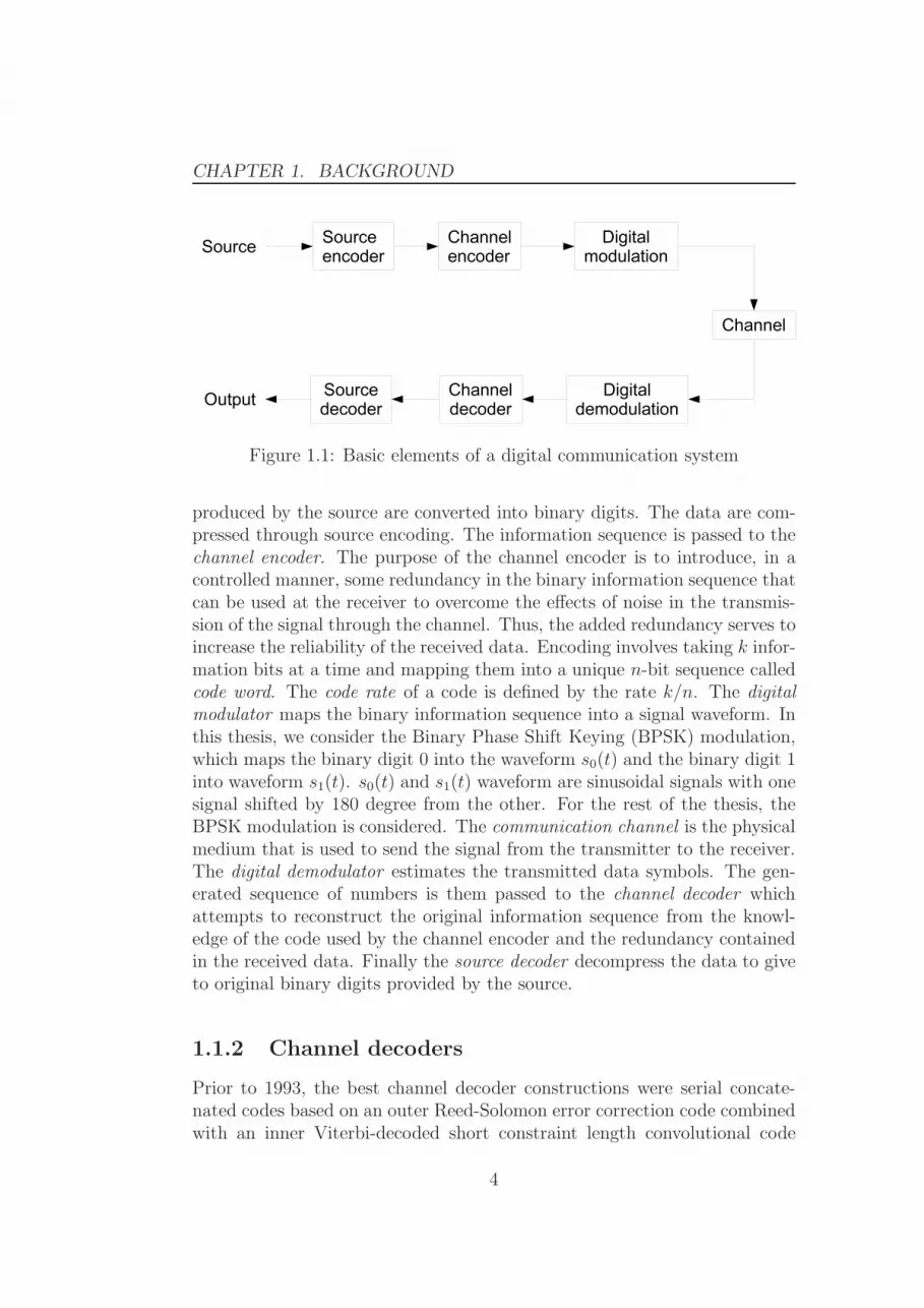
Figure 1.1 illustrates the functional diagram and the basic elements ofa digital communication system. In a digital communication, the messages
3
CHAPTER 1. BACKGROUND
Figure 1.1: Basic elements of a digital communication system
produced by the source are converted into binary digits. The data are com-pressed through source encoding. The information sequence is passed to thechannel encoder. The purpose of the channel encoder is to introduce, in acontrolled manner, some redundancy in the binary information sequence thatcan be used at the receiver to overcome the effects of noise in the transmis-sion of the signal through the channel. Thus, the added redundancy serves toincrease the reliability of the received data. Encoding involves taking k infor-mation bits at a time and mapping them into a unique n-bit sequence calledcode word. The code rate of a code is defined by the rate k/n. The digitalmodulator maps the binary information sequence into a signal waveform. Inthis thesis, we consider the Binary Phase Shift Keying (BPSK) modulation,which maps the binary digit 0 into the waveform s0(t) and the binary digit 1into waveform s1(t). s0(t) and s1(t) waveform are sinusoidal signals with onesignal shifted by 180 degree from the other. For the rest of the thesis, theBPSK modulation is considered. The communication channel is the physicalmedium that is used to send the signal from the transmitter to the receiver.The digital demodulator estimates the transmitted data symbols. The gen-erated sequence of numbers is them passed to the channel decoder whichattempts to reconstruct the original information sequence from the knowl-edge of the code used by the channel encoder and the redundancy containedin the received data. Finally the source decoder decompress the data to giveto original binary digits provided by the source.
1.1.2 Channel decoders
Prior to 1993, the best channel decoder constructions were serial concate-nated codes based on an outer Reed-Solomon error correction code combinedwith an inner Viterbi-decoded short constraint length convolutional code
4

1.1. BASIC CONCEPTS
(used in the DVB-T standard [17]). In 1993, turbo codes were introducedby C. Berrou, A. Glavieux, and P. Thitimajshima (from Telecom-Bretagne,former ENST Bretagne, France) [3]. In a later paper [2], C. Berrou writes“R. Gallager and M. Tanner had already imagined coding and decoding tech-niques whose general principles are closely related,” although the necessarycalculations were impractical at that time. This is a reference to LDPCcodes that are, like turbo codes, iterative decoders. LDPC codes had beendiscovered by Gallager [25] in 1963 and had been rediscovered by MacKay[41] in 1997. Compared with turbo codes, LDPC codes have simpler pro-cessing requirement and their decoding algorithm is inherently parallel. Forlong frames, LDPC decoders offer better performance than turbo codes. Thismakes LDPC decoders relevant for TV broadcasting standards. LDPC codesare included in the linear block codes family and thus heritate from the linearblock codes proporties.
1.1.3 Linear block codes
A linear code is an error-correcting code for which any linear combination ofcodewords is another codeword of the code. Block codes are one of the twocommon types of channel codes (the other one being convolutional codes),which enable reliable transmission of digital data over unreliable communi-cation channels subject to channel noise. A block code transforms a messageconsisting of a sequence of information symbols over an alphabet into a fixed-length sequence of n symbols, called a code word. In a linear block code,each input message has a fixed length of k < n input symbols. The redun-dancy added to a message by transforming it into a larger code word enablesa receiver to detect and correct errors in a transmitted code word, and torecover the original message. The redundancy is described in terms of itsinformation rate, or more simply in terms of its code rate r = k/n.
1.1.4 LDPC codes
The rediscovery in the nineties of the Turbo codes and, more generally,the application of the iterative process in digital communications led to arevolution in the digital communication community. This step forward ledto the rediscovery of Low Density Parity Check (LDPC) codes, discoveredthree decades before. Several recent standards include optional or mandatoryLDPC coding methods. The first standard that included LDPC was the sec-ond generation Digital Video Broadcasting for Satellite (DVB-S2) standard(ratified in 2005 [18]).
5

CHAPTER 1. BACKGROUND
V N4V N1 V N2 V N3
Mv→c Mc→v
CN1 CN2
Figure 1.2: Tanner graph representation of H
LDPC codes are a class of linear block codes. The name comes from thecharacteristic of their parity-check matrix which contains only a few 1’s incomparison to the amount of 0’s. Their main advantage is that they providea performance which is very close to the theoretical channel capacity [58].An LDPC decoder is defined by its parity check matrix H of M rows byN columns. A column in H is associated to a codeword bit, and each rowcorresponds to a parity check equation. A nonzero element in a row meansthat the corresponding bit contributes to the parity check equation associatedto the node.
The set of valid code words x ∈ C have to satisfy the equation:
xHt = 0, ∀x ∈ C (1.1)
An LDPC decoder can be described by a Tanner graph [63], a graphicalrepresentation of the associations between code bits and parity checks equa-tion. Code bits are shown as so called variable nodes (VN) drawn as circles,parity check equations as check nodes (CN), represented by squares, withedges connecting them accordingly to the parity check matrix. Figure 1.2shows a simple Tanner graph of matrix H .
H =
[
1 1 1 00 1 0 1
]
Through the edge, messages are read by the nodes. A message goingfrom CN to VN is called Mc→v, and a message going from VN to CN iscalled Mv→c.
6

1.1. BASIC CONCEPTS
1.1.5 Standard Belief Propagation LDPC decoding
In this subsection, the soft iterative decoding of binary LDPC codes is pre-sented. The iterative process, first introduced by Gallager [25] and rediscov-ered by MacKay [41] is more known as the Belief Propagation (BP) algo-rithm. This algorithm propagates probability messages to the nodes throughthe edges. The probability gives a soft information about the state (0 or 1)of a VN. In the Log-BP algorithm, the probabilities are in the log domainand are called Log Likelihood Ratio (LLR). The LLRs are defined by thefollowing equation:
LLR = log(P (v = 0)
P (v = 1)
)
(1.2)
where P (v = x) is the probability that bit v is egual to x.The order in which the nodes are updated is called the scheduling. The
schedule proposed by Gallager is known as the flooding schedule [25]. Flood-ing schedule consists in four steps. First step is the initialization. Secondstep is the update of all the check nodes. The third step is the update of allthe variable nodes. The fourth step consists in going back to step two untila codeword is found or a maximum number of iteration is reached. At theend of the iterative process, a hard decision is made on the VN to outputthe codeword. The update of a node means that a node reads the incomingmessages and then updates the outgoing messages. The initialization, theVN update and the CN update are described hereafter. The test to find thecodeword or stopping criteria is described in Section 4.4.3.
Initialization
Let x denote the transmitted BPSK symbol corresponding to a codewordbit, and let y denote the noisy received symbol, then y = z + y where z isa Gaussian random variable with zero mean. Let us assume that x = +1when the transmitted bit is 0 and x=-1 when the transmitted bit is 1. LetLLRin = log p(x=+1|y)
p(x=−1|y)denote the a-priori LLR for the transmitted bit. The
sign of LLRin gives the hard decision on the transmitted bit, whereas themagnitude of LLRin gives an indication on the reliability of the decision: thegreater the magnitude is, the higher is the reliability. On a Gaussian channelLLRin is given by:
LLRin = 2y/σ2
where σ is the variance of the received signal.Decoding starts by assigning the a-priory LLR to all the outgoing edge
Mv→c of every VNs.
7

CHAPTER 1. BACKGROUND
0 1 2 3 4 50
1
2
3
4
5
x
f(x)
Figure 1.3: Representation of the f(.) function defined in equation 1.5
Check node update
The CN update is computed by applying the Bayes laws in the logarithmicdomain. For implementation convenience, the sign (1.3) and the absolutevalue (1.4) of the messages are updated separately:
sign(Mc→v) =∏
v′∈vc/v
sign(Mv′→c) (1.3)
|Mc→v| = f
(
∑
v′∈vc/v
f(|Mv′→c|))
(1.4)
where vc is the set of all the VN connected to the check node CN and vc/v is vcwithout v. The f(.) function is expressed by Equation (1.5) and representedin Figure 1.3.
f(x) = − ln tanh(x
2) = ln
exp x+ 1
exp x− 1(1.5)
Variable node update
The VN update is split in two equations (1.6) and (1.7) to show the SoftOutput (SO) value also called the A Posteriori Probability (APP). The SO
8

1.2. SUB-OPTIMAL ALGORITHMS
is calculated in (1.6) where the LLRin value is the initial soft input. Thenfrom this SO, the new Mv→c are computed by (1.7).
SOv = LLRin +∑
c∈cv
Mc→v (1.6)
Mv→c = SOv −Mc→v (1.7)
The VN update is simple and with straight forward implementation. Thecheck node update is more complex and with many possible sub-optimalalgorithm and implementation options which are discussed in the next section
1.2 Sub-optimal algorithms
The f(x) function described in equation (1.5) and used in (1.4) is difficultto implement.This function can be implemented us- ing look up table orlinear pieceware approximation as in [33] but can also be implemented moreefficiently by using a sub-optimal algorithm. The most used algorithms areimproved version of the well known Min-Sum algorithm [24], such as thenormalized min-sum algorithm [11], the offset min-sum algorithm [11], the λ-min algorithm [29] or the Self-Corrected Min-Sum algorithm [55].
1.2.1 The normalized Min-Sum algorithm and other
related algorithms
A lot of researches tend to reduce computational complexity by simplifyingthe Check Node Processor (CNP). The Min-Sum algorithm is the simplestdecoding method which approximates the sum-product algorithm by ignoringother terms except the most minimum incoming message. Therefore thecomplex computation of function f(x) can be eliminated. The CN Min-Sumprocessing of Min-Sum algorithm can be expressed as:
|Mnewc→v| ≈ min
v′∈vc/v|Mv′→c| (1.8)
The Min-Sum algorithm can dramatically reduce the computation com-plexity. However, the resulting approximated magnitude is always overesti-mated. This inaccurate approximation causes significant degradation on thedecoding performance. In the Normalized Min-Sum (NMS) algorithm [11],the output of the CN processor is multiplied by a normalization factor α.This compensates the overestimation of Min-Sum approximation:
9
CHAPTER 1. BACKGROUND
0.5 0.6 0.7 0.8 0.9 1 1.1 1.2 1.3 1.410
−4
10−3
10−2
10−1
100
Eb/Nodb
FE
R
Min−SumNormalized 0.875BPOffset 0.25
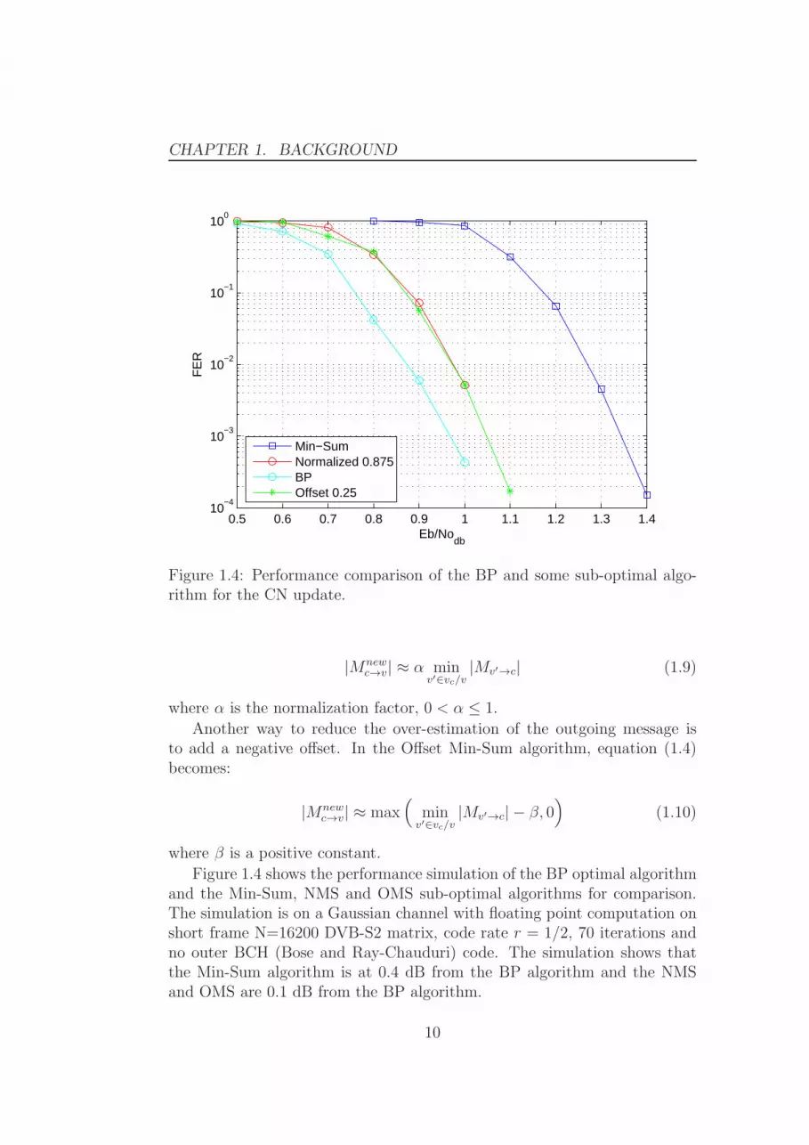
Figure 1.4: Performance comparison of the BP and some sub-optimal algo-rithm for the CN update.
|Mnewc→v| ≈ α min
v′∈vc/v|Mv′→c| (1.9)
where α is the normalization factor, 0 < α ≤ 1.
Another way to reduce the over-estimation of the outgoing message isto add a negative offset. In the Offset Min-Sum algorithm, equation (1.4)becomes:
|Mnewc→v| ≈ max
(
minv′∈vc/v
|Mv′→c| − β, 0)
(1.10)
where β is a positive constant.
Figure 1.4 shows the performance simulation of the BP optimal algorithmand the Min-Sum, NMS and OMS sub-optimal algorithms for comparison.The simulation is on a Gaussian channel with floating point computation onshort frame N=16200 DVB-S2 matrix, code rate r = 1/2, 70 iterations andno outer BCH (Bose and Ray-Chauduri) code. The simulation shows thatthe Min-Sum algorithm is at 0.4 dB from the BP algorithm and the NMSand OMS are 0.1 dB from the BP algorithm.
10

1.2. SUB-OPTIMAL ALGORITHMS
Algorithm name CN update
log-BP |Mc→v| = f
(
∑
v′∈vc/v
f(|Mv′→c|))
Min-Sum [24] |Mc→v| ≈ minv′∈vc/v
|Mv′→c|
Offset Min-Sum [11] |Mc→v| ≈ max(
minv′∈vc/v
|Mv′→c| − β, 0)
Normalized Min-Sum [11] |Mc→v| ≈ α minv′∈vc/v
|Mv′→c|
λ-Min [29] |Mc→v| ≈ f
(
∑
v′∈vλc /v
f(|Mv′→c|))
IF v = argminv′∈vc |Mv′→c| THEN
A-min* [35] |Mc→v| ≈ f
(
∑
v′∈vc/v
f(|Mv′→c|))
ELSE
|Mc→v| ≈ f(
∑
v′∈vcf(|Mv′→c|)
)
IF sign(M tmpv′→c) 6= sign(Mold
v′→c)Self-Corrected Min-Sum [55] THEN Mv′→c = 0
ELSE Mv′→c = M tmpv′→c
|Mc→v| ≈ minv′∈vc/v
|Mv′→c|
Table 1.1: Check node update with different sub-obtimal algorithms
In the λ-min algorithm [29] only the λ most minimum Mc→v values arecomputed. Let vλc be the subset of vc which contains the λ VNs linked toCN c and having the smallest LLR magnitude. Let vλc /v be vλc without VNv. Equation 1.4 is then approximated by:
|Mc→v| ≈ f
(
∑
v′∈vλc /v
f(|Mv′→c|))
(1.11)
Two cases will occur: if the VN belongs to the subset vλc , then the Mv→c
are processed over λ − 1 values of vλc /v, otherwise the Mv→c are processedover the λ values of vλc .
The Self-Corrected Min-Sum algorithm presented in [55] modifies the vari-able node processing by erasing unreliable Mv→c messages.
Table 1.1 summarizes the different sub-optimal algorithms for the CNupdate.
11

CHAPTER 1. BACKGROUND
The advantages of these algorithms are the simplified computation ofequation (1.17) and the compression of the Mc→v messages. Instead of stor-ing all the Mc→v messages conected to one CN, two absolute values, the in-dex of the minimum value and sign of the Mc→v messages need to be stored.This compression lead to significant memory saving with check node degreegreater than 4. Although all these algorithms present different performances,the memory space they require to store the Mc→v messages is identical (con-sidering λ = 2 for the λ-min algorithm). Hence, without loss of generality,for the rest of the thesis, we will consider in the NMS algorithm.
An implementation of the NMS algorithm can be easily improved to aλ-min algorithm or A-min* algorithm by adding look up tables. Many otherimprovements to the Min-Sum algorithm are proposed in the litterature.In[40], a self compensation technique update the normalization factor α as afunction of the CN incoming messages. Because of the massive required com-putation, the method is simplified in [64] by defining a normalization factorfor the min value αmin and an other factor for the other value. Furthermore,the factor is shunted after some iteration to improve the performance.
From the algorithms presented in table 1.1, The NMS algorithm is chosenfor the following reasons:
• performance close to the BP algorithm
• easy implementation
• low implementation area
• extrinsic memory compression
• not sensitive to scaling in the LLRin values
• possibility to improve performance by upgrading to A-min*,λ-min orSelf-Corrected Min-Sum algorithm
1.2.2 Serial implementation of the NMS algorithm
The CN generates two different values: min and submin. The min value isthe normalized minimum of all the incoming Mv→c values and the submin isthe second normalized minimum. Let indmin be the index of min i.e.,
indmin = arg minv′∈vc/v
|Mv′→c|
For each |Mnewc→v| values, if the index of Mnew
c→v is indmin then |Mnewc→v| = submin
else |Mnewc→v| = min. The Mc→v from one CN can be compressed with four
12

1.2. SUB-OPTIMAL ALGORITHMS
elements, i.e. min, submin, indmin and sign(Mnewc→v). For matrices with a
check node degree greater than four, memory saving becomes significant.
To compute the sign, the property that the XOR of “all but one”, is equalto the XOR of “all plus the one” is used, i.e.
⊕
v′∈vc/v
xv′ =⊕
v′∈vc
xv′ ⊕ xv (1.12)
where xv is a sign bit (0 for a positive value and 1 for negative value). Thesign calculation of the outgoing messages is done in two steps. First, all theincoming messages are read. The recursive property of the XOR function:
dc⊕
i=1
xi = xdc ⊕ (xdc−1 ⊕ (xdc−2 ⊕ (xdc−3 ⊕ (· · · ⊕ (x1) · · · )))) (1.13)
is used to compute the XOR of all the incoming messages serially. In thesecond step, the sign of the outgoing messages are computed serially byapplying equation (1.12).
To compute the magnitude, the first step consists in a serial sorting of theincoming value to produce the min, submin and indmin values. During thesecond step, the min, submin and indmin values are used to serially computethe outgoing magnitude messages.
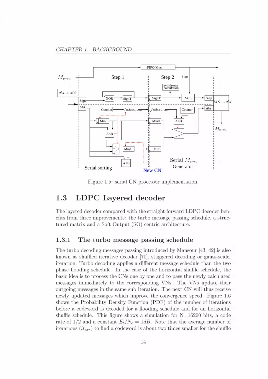
Figure 1.5 shows the serial CN processor implementation. The Mv→c
values arrive serially in a two’s complement form and are transformed insign and magnitude representation to be computed separately. The figure issplit horizontally and vertically: the upper part is for the sign computationand lower part for the magnitude computation. The left part represents thefirst step computation and the right part the second step. The upper part isa straight forward implementation of the sign computation where signT =⊕dc
i=1xi. The upper left part implement equation (1.13) in a first step. Thenthe right upper part implements equation (1.12) for the second step. Thelower part implement the magnitude computation with in a first step, thesorting of the incoming magnitude in order to store the min, submin andindmin values until all the incoming messages are read. Then in the secondstep (lower right part) the min, submin and indmin values previously sortedare used to serially compute the new outgoing messages. Then, the sign andmagnitude are transformed in two’s complement for later computation. Step1 and step 2 take dc cycles to process and can easily be pipelined.
13
CHAPTER 1. BACKGROUND
XOR
A<B
A<B
symdromecalculation
Sign
Abs
Min0
Min1
Generator
Min0
Min1
A=B
CounterCounter
Serial sorting
FIFO Mvc
Abs
Sign
Sign
New CN
Step 2Step 1
SignTSignTXOR
IndexMin0 IndexMin0
Serial Mc→v
2′s → MS
Mv→c
Mc→v
MS → 2′s
Figure 1.5: serial CN processor implementation.
1.3 LDPC Layered decoder
The layered decoder compared with the straight forward LDPC decoder ben-efits from three improvements: the turbo message passing schedule, a struc-tured matrix and a Soft Output (SO) centric architecture.
1.3.1 The turbo message passing schedule
The turbo decoding messages passing introduced by Mansour [43, 42] is alsoknown as shuffled iterative decoder [70], staggered decoding or gauss-seideliteration. Turbo decoding applies a different message schedule than the twophase flooding schedule. In the case of the horizontal shuffle schedule, thebasic idea is to process the CNs one by one and to pass the newly calculatedmessages immediately to the corresponding VNs. The VNs update theiroutgoing messages in the same sub iteration. The next CN will thus receivenewly updated messages which improve the convergence speed. Figure 1.6shows the Probability Density Function (PDF) of the number of iterationsbefore a codeword is decoded for a flooding schedule and for an horizontalshuffle schedule. This figure shows a simulation for N=16200 bits, a coderate of 1/2 and a constant Eb/No = 1dB. Note that the average number ofiterations (itavr) to find a codeword is about two times smaller for the shuffle
14

1.3. LDPC LAYERED DECODER
0 10 20 30 40 50 60 70 800
0.02
0.04
0.06
0.08
0.1
0.12
0.14
0.16
iteration
Pro
babi
lity
floodinghorizontal
itmax
itmax
itavr
itavr
Figure 1.6: Probability Density Function of the number of iterations beforea codeword is found
schedule than for the flooding schedule. The same observation can be donefor the maximum number of iterations (itmax).
However, the main drawback of this schedule is that the CN are updatedserially one by one leading to low throughput. The next subsection explainshow this serial schedule can be partially parallelized.
1.3.2 Structured matrices
The semi-parallel horizontal Shuffle decoder is also known as Group hori-zontal Shuffle or Layered Horizontal shuffle [53]. Layered decoding uses thesame principle as the Turbo decoding but instead of processing the CNs oneby one, they are processed by groups. Let P be the size of the group. ThenP CN are processed in parallel. This is possible only if the weights of thecolumns in a block does not exced one. The idea is to use identity matricesof size P×P . The IEEE WiMAx standard [60] uses this structure and is wellexplained in [10] where an efficient architecture is also presented. Figure 1.7shows the structure of the rate-2/3 short-frame DVB-S2 LDPC parity checkmatrix. This structured matrix is composed of shifted identity matrices ofsize P = 360, allowing for efficient parallel processing of up to 360 CNs.
15

CHAPTER 1. BACKGROUND
0 720 10,800 16,200
0360720
3,600
5,400
CN
m
V Nn
Figure 1.7: Block-structured rate-2/3 DVB-S2 matrix (N=16200 bits)
1.3.3 Soft Output (SO) centric decoder
In this subsection we explain how the soft output (SO) based check nodeprocessor (CNP) architecture is deduced. From (1.6) and (1.7), we can findthe new equation:
SOv = Mv→c +Mc→v (1.14)
The update of the VNs connected to a given CN is done serially in threesteps. First, the message from a VN to a CN (Mv→c) is calculated as:
Mv→c = SOv −Moldc→v (1.15)
The second step is the serial Mc→v update, where Mc→v is a message from CNto VN, and is also called extrinsic. Let vc be the set of all the VNs connectedto CN c and vc/v be vc without v. For implementation convenience, the signand the absolute value of the messages |Mnew
c→v| are updated separately:
sign(Mnewc→v) =
∏
v′∈vc/v
sign(Mv′→c) (1.16)
|Mnewc→v| = f
(
∑
v′∈vc/v
f(|Mv′→c|))
(1.17)
where f(x) = − ln tanh(
x2
)
. The third step is the calculation of the SOnew
value:SOnew
v = Mv→c +Mnewc→v (1.18)
The updated SOnewv value can be used in the same iteration by another sub-
iteration leading to convergence which is twice as fast as the flooding schedule[42].
16

1.3. LDPC LAYERED DECODER
CNP
++−
NP
SOv SOnewv
Mv→c
Mc→vMnew
c→vMold
c→v
Figure 1.8: SO based Node Processor
1.3.4 Architecture overview
From equations (1.15) to (1.18), the Node Processor (NP) architecture Fig.1.8 can be derived. The left adder of the architecture performs equation(1.15) and the right adder performs equation (1.18). The central part is incharge of the serial Mc→v update.
As the structured matrices are made of identity matrices of size P , P CNsare computed in parallel. Hence, the layered decoder architecture is basedon P NPs that first read serially the Groups of P VNs linked to one layerand then write back the SOnew
v in the VNs.The architecture proposed in Figure 1.9 is mainly based on the archi-
tecture of a layered decoder. The counter counts up to IMbase (i.e. thenumber of identity matrices in the base matrix). The ROM linked to thecounter delivers the V Gread
i addresses and the associated shift value Shiftifollowing the base matrix order. The V Gwrite
i adresse is given by V Greadi
which is delayed by dc + ǫ cycles corresponding to latency to compute a newSO value. The size of the ROM dedicated to store V Gi and Shifti is thusIMbase × (log2(N/P ) + log2(P )).
Usually, a barrel shifter is in charge of shifting the SO values by Shifti be-fore being processed, and after processing, another barrel shifter is in chargeof shifting back the SO values in memory. In this architecture, the ∆Shiftgenerator allows using one barrel shifter instead of two.
As there is no barrel shifter in charge of shifting back the SO values, atthe next call of a VNG, the SOs in this group are already shifted by the shiftvalue of the previous call (Shiftoldi ). The ∆Shift value takes into accountthe shift value of the previous calls by doing the subtraction ∆Shifti =Shiftnewi − Shiftoldi . Shiftold is stored in a RAM of size N/P × log2(P ).
The Mv→c memory is implemented using a FIFO of size dc. For the SO
17

CHAPTER 1. BACKGROUND
IM number
RAMShift
Counter
Address
VGn Shift
ROM
+
−
−
+ +SORAM
Bar
rel S
hifte
r
NPPs
×Ps
ShiftoldShiftnew
Mc→v
Mv→c
∆shift
V GreadiV Gwrite
i
D−(dc+ǫ)
Figure 1.9: Layered decoder architecture
RAM, a dual-port RAM with one port for writing and another for readingis required for pipelining.
Figure 1.10 presents the detailed architecture of the CN update and theMc→v memory for the implementation of the NMS algorithm. Note that thearchitecture includes the NMS update described in Figure 1.5.
1.4 The DVB-S2, -T2 and -C2 standards
1.4.1 Digital Terrestrial Television
With the establishment of the European Digital Video Broadcasting (DVB)standard and the American Television Systems Committee (ATSC) standard,digital TV (DTV) broadcasting is now a reality in several countries. The Ter-restrial broadcasting or Digital Terrestrial Television (DTT), in France the”Television numerique terrestre” (TNT) are defined by the DVB-T standard[19]. Even if DTT requires a set top box equipment or a specific chip inthe TV, it offers many advantages. Among them, thanks to the ForwardError Correction (FEC), DTT allows obtaining optimum picture when ananalogue tuner would only allow a poor quality picture. With DTT, thehigh definition television (HDTH) is also possible. The format is the 1920by 1080 pixel/frame format interlaced at 60 fields per second.
18

1.4. THE DVB-S2, -T2 AND -C2 STANDARDS
SignT
+
+
−RAM_SO
Bar
el S
hifte
r
GeneratorIndex
Min_1
Min_0
Sign
RA
M(M
/P)
FIFO(Dc)
SortingSerial
XOR
Serial
generator
Check node core
$VG_i^{read}$VG_i^{write}
∆Shift
2′s→
SM
SerialMc→v
SM
→2′s
|Mc→v |
SM
→2′s
MC→V memory
Mv→c
Figure 1.10: Detailed SO based Node Processor
1.4.2 DVB group
The DVB Project, founded in September 1993, is a consortium of public andprivate sector organizations in the television industry. Its aim is to estab-lish the framework for the introduction of MPEG-2 based digital televisionservices. Now comprising over 200 organizations from more than 25 coun-tries around the world, DVB fosters market-led systems, which meet thereal needs, and economic circumstances, of the consumer electronics and thebroadcast industry.
DVB-S (EN 300 421 [17]) was introduced as a standard in 1994 and DVB-DSNG (EN 301 210 [18]) in 1997. The DVB-S standard specifies QPSK mod-ulation and concatenated convolutional and Reed-Solomon channel coding,and is now used by most satellite operators worldwide for television and databroadcasting services. In addition to DVB-S format, the DVB-DSNG spec-ifies the use of 8PSK and 16QAM modulation for satellite news gatheringand contributing services.
The new standard for digital video broadcast features a powerful FECsystem which enables transmission close to the theoretical limit (Shannonlimit). DVB-S2 is a single and very flexible standard which covers a varietyof applications by satellite and among them, a powerful FEC system basedon LDPC codes concatenated with BCH codes, allowing Quasi-Error-Freeoperation at about 0,7dB to 1 dB from the Shannon limit, depending onthe transmission mode (AWGN channel, modulation constrained Shannonlimit). The 2nd Generation Terrestrial DVB (DVB-T2) standard adopted in2009 and the 2nd Generation Cable DVB (DVB-C2) adopted in 2010 include a
19

CHAPTER 1. BACKGROUND
Standard lenght code rates
DVB-S2 short 1/4, 1/3, 2/5, 1/2, 3/5, 2/3, 3/4, 4/5, 5/6, 8/9long 1/4, 1/3, 2/5, 1/2, 3/5, 2/3, 3/4, 4/5, 5/6, 8/9, 9/10
DVB-T2 short 1/4, 1/2, 3/5*, 2/3, 3/4, 4/5, 5/6long 1/2, 3/5, 2/3*, 3/4, 4/5, 5/6
DVB-C2 short 1/2, 2/3, 3/4, 4/5, 5/6, 8/9long 2/3*, 3/4, 4/5, 5/6, 9/10
Table 1.2: code rates for DVB-S2, -T2, -C2 standards
common Forward Error Correction (FEC) block with the DVB-S2 standard.
1.4.3 The LDPC code in the DVB-S2, -T2 and -C2standards
The DVB-S2, -T2, -C2 standards features variable coding and modulation tooptimize bandwidth utilization based on the priority of the input data, e.g.,SDTV could be delivered using a more robust setting than the correspond-ing HDTV service. These DVB standadards also features adaptive codingand modulation to allow flexibly adapting transmission parameters to thereception conditions of terminals, e.g., switching to a lower code rate duringfading.
Code rates
The DVB-S2, -T2, -C2 standards [20, 22, 21] are characterized by a widerange of code rates (from 1/4 up to 9/10) as shown in table 1.2. Further-more, FEC frame may have either 64800 bits (normal) or 16200 bits (short).Each code rate and frame length corresponds to an LDPC matrix: this is 21matrices for the DVB-S2 standard, 13 matrices for the DVB-T2 standard and11 matrices for the DVB-C2 standard. The matrices construction is identicalfor the three standards. The advantage is that the same LDPC decoder canbe used for the 3 standards. Due to the fact that the decoder is identical forthe 3 standards, hereafter DVB-X2 refers to DVB-2, -T2, -C2 standards.
Matrix construction
LDPC codes can be specified through their parity check matrices. The DVB-X2 LDPC codes are 64800 bits long. Therefore, a certain structure is imposed
0*upgraded matrix with better performance compared to DVB-S2 standard
20
1.4. THE DVB-S2, -T2 AND -C2 STANDARDS
on parity check matrices to facilitate the description of the codes and theencoding.
By inspecting the construction rules in [20, 22, 21], the DVB-S2, -T2 and-C2 parity check matrices consist in two distinctive parts: a random partdedicated to the systematic information, and a fixed part that belongs to theparity information. Two types of VN can be distinguished: the InformationVN (IVN) and the Parity VN (PVN) corresponding to the systematic andparity bits respectively. The connectivity between every IV Nm and CNj isdefined by the standard encoding rule:
CNj = CNj ⊕ IV Nm, j = (x+ q(m mod 360)) mod M. (1.19)
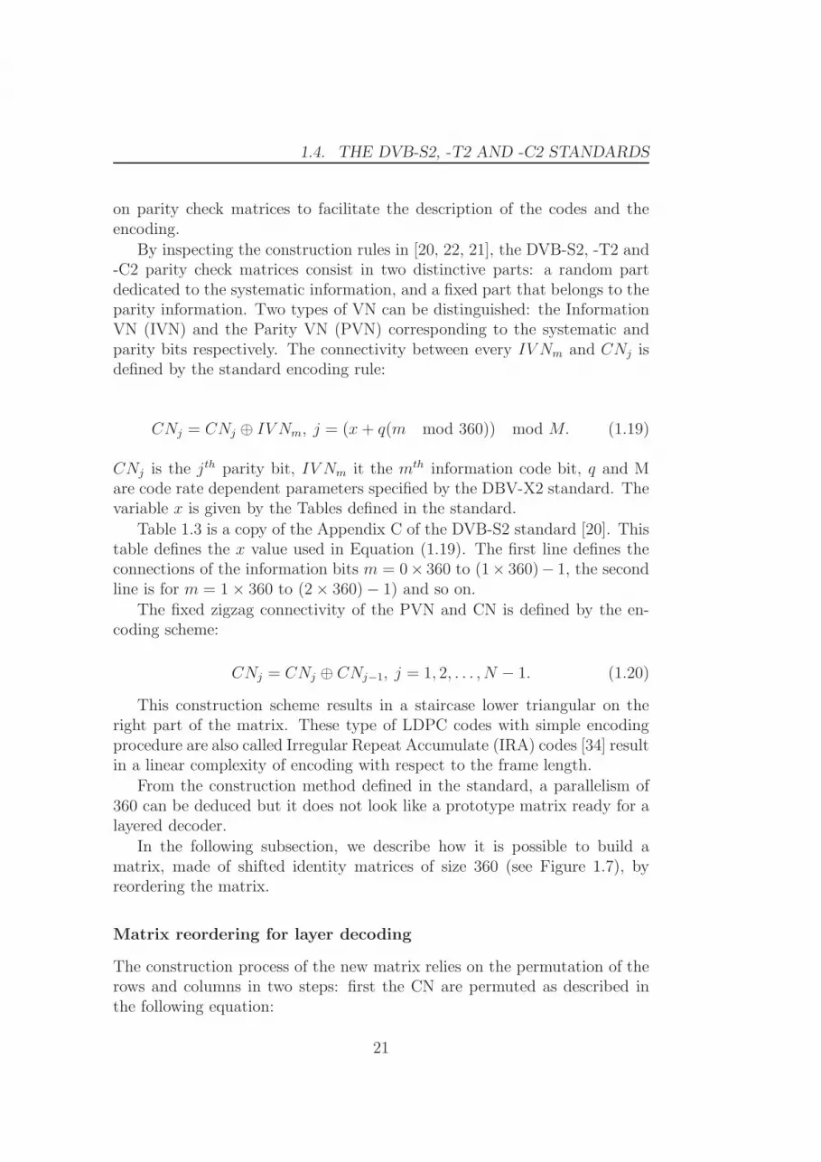
CNj is the jth parity bit, IV Nm it the mth information code bit, q and Mare code rate dependent parameters specified by the DBV-X2 standard. Thevariable x is given by the Tables defined in the standard.
Table 1.3 is a copy of the Appendix C of the DVB-S2 standard [20]. Thistable defines the x value used in Equation (1.19). The first line defines theconnections of the information bits m = 0× 360 to (1× 360)− 1, the secondline is for m = 1× 360 to (2× 360)− 1) and so on.
The fixed zigzag connectivity of the PVN and CN is defined by the en-coding scheme:
CNj = CNj ⊕ CNj−1, j = 1, 2, . . . , N − 1. (1.20)
This construction scheme results in a staircase lower triangular on theright part of the matrix. These type of LDPC codes with simple encodingprocedure are also called Irregular Repeat Accumulate (IRA) codes [34] resultin a linear complexity of encoding with respect to the frame length.
From the construction method defined in the standard, a parallelism of360 can be deduced but it does not look like a prototype matrix ready for alayered decoder.
In the following subsection, we describe how it is possible to build amatrix, made of shifted identity matrices of size 360 (see Figure 1.7), byreordering the matrix.
Matrix reordering for layer decoding
The construction process of the new matrix relies on the permutation of therows and columns in two steps: first the CN are permuted as described inthe following equation:
21
CHAPTER 1. BACKGROUND
0 2084 1613 1548 1286 1460 3196 4297 2481 3369 3451 4620 26221 122 1516 3448 2880 1407 1847 3799 3529 373 971 4358 31082 259 3399 929 2650 864 3996 3833 107 5287 164 3125 23503 342 35294 4198 21475 1880 48366 3864 49107 243 15428 3011 14369 2167 251210 4606 100311 2835 70512 3426 236513 3848 247414 1360 17430 163 25361 2583 11802 1542 5093 4418 10054 5212 51175 2155 29226 347 26967 226 42968 1560 4879 3926 164010 149 292811 2364 56312 635 68813 231 168414 1129 3894
Table 1.3: matrix construction table for DVB-S2 standard, code rate of 2/3and short frame lengh
22

1.4. THE DVB-S2, -T2 AND -C2 STANDARDS
V Gng
CG
mg
5 10 15 20 25 30 35 40 451
123456789
101112131415
Figure 1.11: Base DVB-S2 matrix representation
σ(j+ i×360) = i+(j× q) mod N, i = 1, 2 . . . , q, j = 1, 2, . . . , 360. (1.21)
Then the PVN are permutated by following the same permutation equa-tion. The obtained matrix is made of Identity Matrix (IM) sized 360.
The matrix construction and permutation process is illustrated in ap-pendix A. Figure 1.11 illustrates the IM in the rate-2/3 short-frame matrix.V Gi denotes the i
th group of 360 VNs and CGj denotes the jth group of 360
CNs. A square denotes a permuted IM linking CGj and V Gi. Let im bethe identity matrix number. Each IM (im = 1, 2, . . . , IM total) can be bestdescribed by giving the shift value δIMim and the coordinate of the IM in thematrix which is given by the CGIM
im value and the V GIMim value.
There is a convenient way to obtain directly the shift value δIMim , and theaddress (CGIM
im and V GIMim ) values from the standard value x given in the
standard table 1.3. In this table, each x value corresponds to an identitymatrix. The line number corresponds to the VG number V GIM
im = line. Theshift value of each im is given by:
δIMim = (360− ⌊x/q⌋) mod 360. (1.22)
and the check group number is given by:
CGIMim = x mod q. (1.23)
23

CHAPTER 1. BACKGROUND
The connectivity of the PVN and CN is built by a staircase of identitymatrices as in Figure 1.11(V G31toV G45). Each identity matrix in the stair-case has a shift value of 0. The up right IM is a special IM with a shift of359 and the up right connectivity removed.
The permutation of the matrices allows obtaining a structured matrixready to be used by a layered decoder. The DVB-S2 standard was the firststandard including an LDPC decoder and many different implementationoptions have been tested in the State of the art.
1.4.4 State-of-the-art on DVB-S2 LDPC implementa-
tion
To our knowledge, the first implementation presented by F. Kienle et al[36] with synthesis results, benefits from the parallelism of P = 360. Theimplementation relies on a flooding schedule and an optimized update of CNof degree 2. Due to the varying node degree, the functional CN units processall incoming messages in a serial manner. This serial processing of the comingmessages is a common point to most implementations recorded in our stateof the art. Although it was able to provide a throughput far above from themandatory rate of 90 Mbps, the high number of processing units and thelong width of the barrel shifter require a huge silicon area. The throughputof this first implementation was more than required by the standard.
In [14],[27] the parallelism is reduced to any integer factor of 360 by usingan efficient memory bank partitioning.
In all implementations recorded, the shuffling network implementation isbased on the use of barrel shifters. The differentiation comes from the sizeand the number of shuffling networks. The size of the shuffling network willdepend on the parallelism. In [14, 36] two shuffling networks are used (onefor shuffle and the other to shuffle back), while in [27] the author saves oneshuffling network. In [27] instead of shuffle back the data, the shift value ismemorized and thanks to the linearity of the barrel shifter, the next shiftvalue is computed by a simple substraction.
In [14] the authors presented the first implementation that benefit fromlayered decoder architecture. Implementations of layered decoder are alsopresented in [57, 68, 48, 66, 65]. A layered decoder requires matrices madeof IM, but in the case of the DVB-X2 matrices, the superposition of ma-trices appears. The superposed matrices are not compatible with a layereddecoder leading to conflicts and a patch is mandatory to solve the problem.In [57, 48], the problem is identified and solved by the computation of themessage variation. The problem is also solved by using a ’delta’ architecture
24
1.5. TESTING THE PERFORMANCE OF A DECODER
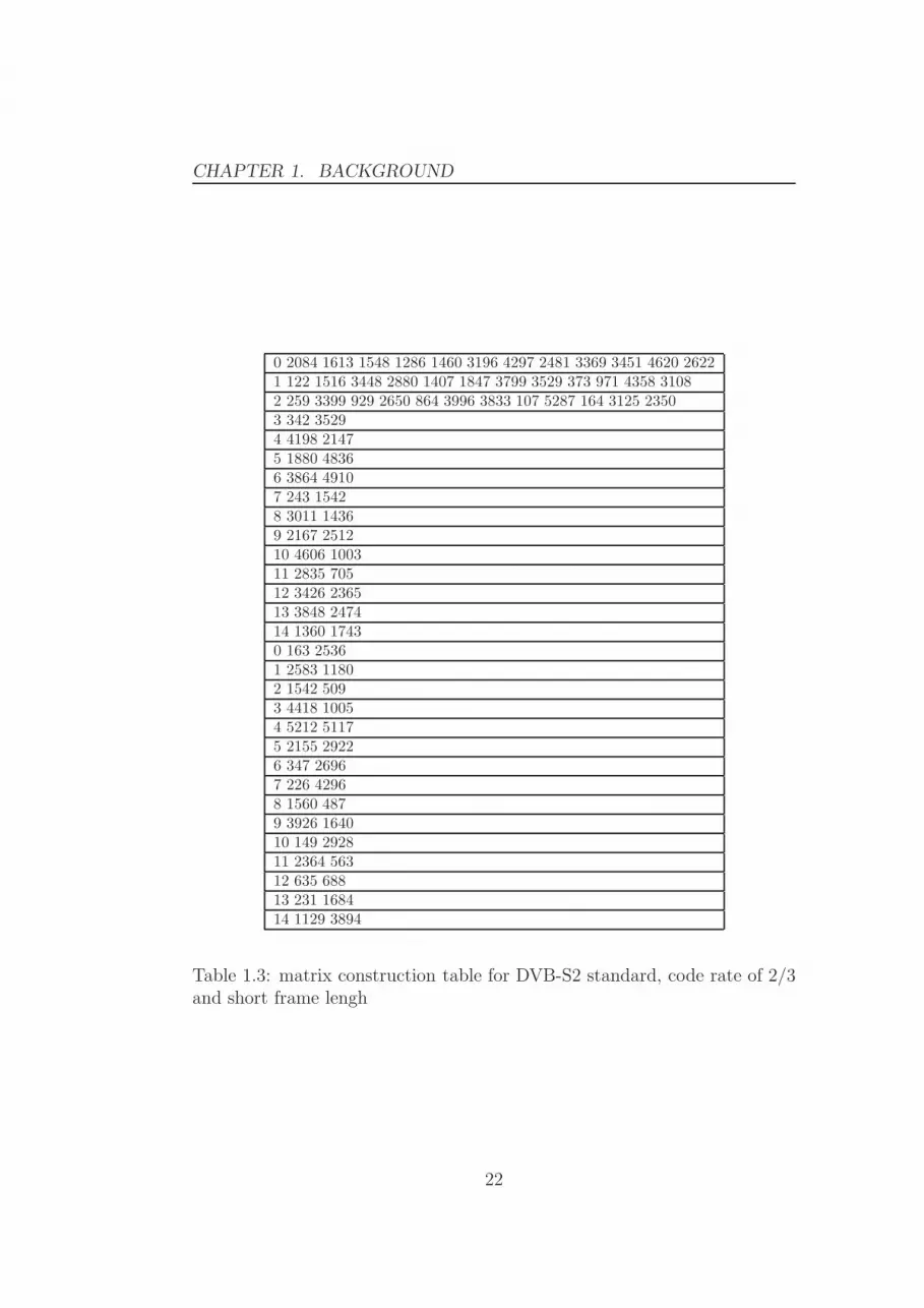
Figure 1.12: Block diagram of a testing environment
as described in [8] and in [53]. These solutions are efficient but comparedto a standard layered decoder requires another access to the SO memory tocompute the new SO (SOnew = SOold + delta) which is costly in terms ofmemory size.
A vertical layer schedule version of the layered decoder is proposed in [47].This architecture allows iterative message passing between the de-mapperand the LDPC decoder. In [23] an alternative approximation of CN algorithmfor DVB-S2 LDPC decoder is proposed. The alternative approximation isbased on the first series approximation of equation (1.5), the magnitudeupdate of the |Mc→v| is expressed with log2(x) and 2x function which can beeasily implemented by a shifter and apriority encoder.
From this state of the art, the choice of a layered decoder has been de-cided. Based on this choice, the research is focused on an efficient solutionfor the memory conflicts and an optimized implementation in term of areaand consumption. In this thesis, a testing environment has been developedto test the performance of the different solutions. This testing environmentis described in the next section.
1.5 Testing the performance of a decoder
Advanced digital wireless communication systems often require an appropri-ate trade-off between complexity and performance of an efficient iterativedecoder design. In practice, from the floating point to the fixed-point hard-ware description, many parameters (reliability message length, digital wordsize, rounding and quantization operations, etc.) should be jointly optimized.However, these parameters interact in a non-linear way and the selection ofthe optimal algorithm is a very high time-consuming task. Usually, the ex-
25

CHAPTER 1. BACKGROUND
pression of Bit Error Rate (BER) or the Frame Error Rate (FER) expressedin [50] is used to predict the performance of the system. The conventionalsolution is the Monte-Carlo simulation that evaluates the BER, which givesan estimation of the error correcting capability of the decoder. Figure 1.12shows block diagrams of a testing environment using Monte-Carlo simulation.The source is random and the noise has a Gaussian distribution of variancedepending on the Eb/N0 ratio. In this section, two practical applications arepresented to test an LDPC decoders.
1.5.1 Software and hardware simulation
The Monte-Carlo simulation method is traditionally performed by softwareprograms. With this approach, a FER around 10−9 requires one or two weeksof simulation. To speed up these very long simulations, some software ap-proaches are proposed, such as, a reduced Monte-Carlo simulation method[7] that re-runs only erroneous codewords obtained from an initial ”classical”Monte-Carlo simulation. In [59] is proposed a technique called the distance-based method which is based on the direct evaluation of a distance betweenthe soft output of the sub-optimal decoder and the soft output of a referencedecoder. Although these methods reduce the simulation time, the softwarebased execution (for instance, executing applications on a conventional CPUcluster) is still costly due to the high power consumption and physical spacecost. Consequently, the solution used for this thesis is simulation by us-ing a hardware accelerator based simulation. To combine the high speed ofhardware simulation and the flexibility of software simulation, the testingenvironment is designed to be able to switch from software to hardware sim-ulation at any time for C-VHDL co-simulation. Another advantage of thissolution is the use of co-simulation for debugging.
1.5.2 Test with all-zero codewords
Due to the linearity of the LDPC decoder, we can consider an ’all zero code-word’ with a Binary Phase-Shift Keying (BPSK) transmission on a Gaussianchannel. Fig. 1.13 shows the all zero codeword model for the test of FERor/and BER. The channel emulator block is in charge of adding a noise tothe signal to emulate a noisy channel. For a Gaussian channel, an AdditiveWhite Gaussian Noise (AWGN) is added to the signal as in [6, 39]. We pre-sented in [9] an Hardware Discrete Channel Emulator (HDCE) which is moredetailed in Appendix B. In the compute errors block linked with the decoderoutput, each non-zero value is counted as a bit error. With the bit errors,the BER and FER are easily deduced and the index (SNR) is incremented
26

1.5. TESTING THE PERFORMANCE OF A DECODER
Compute errors
Channel emulator
LDPC decoder
Channel
Display
Eb/No User
FERBER
Frame
Result
deserializer
Figure 1.13: Test of an LDPC decoder, all-zero codeword model
when a maximum number of frame errors is reached. The testing environ-ment including the HDCE is low cost and easy to design. The test patch canbe included as a part of a decoder chip or IP for built-in SNR estimation andtesting purposes at a low area cost. It would take less than 2% of the areaof a DVB-S2 LDPC decoder described in [48] .
1.5.3 Test of a communication model
To get closer to a real communication, or to test the encoder, the test of theperformance of the LDPC codes in a communication model becomes relevant.In Figure 1.14, the codeword from the encoder is sent serially to emulate aBPSK modulation on the AWGN channel. The FIFO stores the source wordsuntil the codeword is decoded. Then the compute errors block compares thetwo words and deduces bit errors. This model has been used to test a nonbinary LDPC code in the DAVINCI project [51].
1.5.4 Channel emulator
To emulate a Gaussian channel, usually an Accurate White Gaussian Noise(AWGN) is added to the signal as in [26, 6, 39]. An alternative is to use
27

CHAPTER 1. BACKGROUND
Compute errors
Channel emulator
LDPC decoder
LDPC encoder
FIFO
Random source
Channel
Display
Eb/No User
FERBER
Frame
Result
deserializer
Figure 1.14: test of an LDPC decoder
the Hardware Discrete Channel Emulator (HDCE) presented in [9] and inAppendix B. The implementation of the HDCE was part of my master’sdegree work. The HDCE directly produce a value with the required distribu-tion. The HDCE relies on the “Alias Method” [67] and the implementationhas been optimized for high speed. The advantages of the HDCE are a re-duced area cost, high speed, the possibility to emulate other channel and thepossibility to replay sequence for debugging.
1.5.5 Interpreting results
The error rate of iteratively decoded codes has a typical shape such assketched in Figure 1.15. Three regions can be easily distinguished. Thefirst region is where the code is not efficient, even if the number of iterationsis increased. The waterfall region is where the error rate has a huge negativeslope. Ideally the waterfall region is vertical. The more the waterfall regionis on the left side, better is the code. The error floor region is where thecurve does not fall as quickly as before. The error floor appears at low BER,and is usually caused by trapping sets or pseudo-codewords. The error floorhas to be at a BER as low as possible for a good code.
28

1.5. TESTING THE PERFORMANCE OF A DECODER
Figure 1.15: Typical regions in an error probability curve
The Shannon limit
Stated by Claude Shannon in 1948, the theorem describes the maximum pos-sible efficiency of error-correcting methods versus level of noise interferenceand data corruption. The Shannon theorem states that given a noisy chan-nel with channel capacity C and information transmitted at a rate R, thenif R < C there exist codes that allows the probability of error at the receiverto be made arbitrarily small. With a given coding rate r, it is possible tocalculate the minimum possible Eb/N0(dB) value.
Eb/N0(min)(dB) = 10 log((22r − 1)/2r) (1.24)
1.5.6 Standard requirements
For the DVB-S2 standard, the standard requirement is to be within 1 dBfrom the Shannon limit at Quasi Error Free (QEF). The definition of QEFadopted for DVB-S.2 is “less than one uncorrected error-event per transmis-sion hour at a level of a 5Mbit/s single TV service decode”, approximatelycorresponding to a Transport Stream Packet Error Ratio PER < 10−7 beforede-multiplexer, where a packet is a MPEG packet of 188 bytes. In this thesis,we will approximate the QEF at FER < 10−6 and BER< 10−10. A simula-tion that gives results within the standard requirement must have the errorfloor threshold at BER< 10−10 and Eb/N0(std)(dB) < Eb/N0(min)(dB)+ 1.
Table 1.4 gives for the code rates used in the DVB-X2 standards theminimum achievable Eb/N0(min)(dB) value computed using equation 1.24.
29

CHAPTER 1. BACKGROUND
code rate 1/4 1/2 2/3 3/4 4/5 5/6 9/10
Eb/N0(min)(dB) -1.9 0 1.3 1.9 2.4 2.6 3.2Eb/N0(std)(dB) -0.9 1 2.3 2.9 3.4 3.6 4.2
Table 1.4: Shannon limit in function of the code rate
Table 1.4 also gives the maximum Eb/N0(std)(dB) value at BER = 10−10
for a simulation to fulfill the standard requirements.
30

Take time to deliberate, but
when the time for action has
arrived, stop thinking and go
in.
Napoleon Bonaparte(1769-1821)
2Memory update conflicts
Summary:In this chapter, a pipelined layered LDPC decoder is considered as the
best implementation solution for the DVB-X2 standard. The major drawbackof using a layered decoder with DVB-X2 standards are the arising memoryupdate conflicts due to the structure of the matrix and the pipelined archi-tecture. Solving these memory conflicts requires efficient strategies to keepperformance, high throughput and low hardware complexity. State-of-the-artsolution includes complex control, hardware patch or idle cycle insertion. Inthis chapter, we propose alternative solutions based on the “divide and con-quer” strategy to overcome the memory conflicts. Two kinds of conflicts areidentified and solved separately: the conflicts due to the matrix structure andthe conflicts due to pipelined architecture. The number of conflict due to thestructure of the matrix is first reduced by a reordering mechanism of the ma-trix called split algorithm that creates a new structured matrix which reducesthe parallelism. Then the remaining conflicts are solved by an equivalent ma-trix using added punctured bits. Another solution based on a repeat of thedeficient layer and an “on time” write disable of the memory offers an evenbetter performance. To solve the conflict due to pipelining, the split processis used again as a first step followed by an efficient scheduling of the layersand identity matrices.
31

CHAPTER 2. MEMORY UPDATE CONFLICTS
0 360 720 1080
0
360
720
CN
m
V Nn
Figure 2.1: Zoom of a rate-2/3 DVB-T2 Matrix with N=16200
A memory update conflict occurs when a data is computed by a pro-cessing unit while this data has not been updated yet by another processingunit. Although DVB-X2 standards define structured parity check matrices,these matrices are not perfectly structured for layered decoder architecture,leading to conflicts in the SO memories. In the beginning of this chapter,our attention is focused on a particular type of conflict introduced by theexistence of overlapped shifted identity matrices in the DVB-X2 parity checkmatrix structure. Then the memory update conflicts introduced by the useof a pipelined CNP are identified and solved by an efficient scheduling.
2.1 Conflicts due to the matrix structure
Figure 2.1 shows a zoom on the first 720 VNs and CNs of the DVB-T2 LDPCmatrix illustrated in Figure 1.7. One can see that the first group of 360 CNsis linked twice to the first group of 360 VNs by two diagonals. The sub-matrices with a double diagonal in it will be called Double Diagonal SubMatrix (DDSM). The DDSM are also called overlapped identity matrices orsuperposed sub-matrices and are also present in the LDPC matrices of theChinese Mobile Multimedia Broadcasting (CMMB) standard [61].
Let us consider the case where two CNs (C1 and C2) are computed in onelayer and connected to the same VN denoted vdd. There are two updates ofthe same SO value. The calculation of the new SO (2.1) is deducted fromequation (1.15) and (1.18). Assuming ∆Mc→v = −Mold
c→v +Mnewc→v and using
(2.1), the calculation of SOnew1vdd
and SOnew2vdd
in (2.2) and (2.3) are obtainedrespectively.
SOnewv = SOold
v −Moldc→v +Mnew
c→v (2.1)
32

2.1. CONFLICTS DUE TO THE MATRIX STRUCTURE
V Gng
CG
mg
5 10 15 20 25 30 35 40 451
123456789
101112131415
Figure 2.2: Base DVB-T2 matrix representation
SOnew1
vdd= SOold
vdd+∆Mc1→vdd (2.2)
SOnew2
vdd= SOold
vdd+∆Mc2→vdd (2.3)
Because the SO is updated serially in the layered architecture, the SOnew2vdd
will overwrite the SOnew1vdd value. This conflict is equivalent to cut theMc1→vdd
message. This is called a cutting edge in [8] and will lead to significant per-formance degradation. With a straightforward implemented layered decoder,each DDSM will produce P cutting edges and dramatically annihilating thedecoding performances.
Figure 2.2 illustrates the number of DDSMs in the rate-2/3 short-framematrix. V Gi denotes the ith group of 360 VNs and CGj denotes the jth
group of 360 CNs. A black square represent a single permuted identitymatrix linking CGj and V Gi and a gray square corresponds to a DDSM.Note that there are 14 DDSMs in this example.
2.1.1 State-of-the-art
Among all the literature about DVB-X2 implementation, the problem ofoverlapped sub-matrices is rarely explicitly identified and solved. In [36],the problem is avoided by applying the Gauss-Seidel technique only on thestaircase part of the parity check matrix. The architecture in [14] applieslayers decoding but does not shows the treatment to superposed sub-matrices.
33

CHAPTER 2. MEMORY UPDATE CONFLICTS
In [53] and [8] the authors present a solution to avoid memory updateconflicts based on the computation of the variation (or delta) of the SOmetrics to allow concurrent updates. The computation of this SO update(SOnew = SOnew +∆Mc→v) requires an additional SO access which is costlyto implement.
In [48], the problem of overlapped matrices is identified and solved bycomputing the variation only in case of overlapped matrices. In the architec-ture proposed the SO update (SOnew = SO + delta) is done locally beforeshifting back in the SO memory. This architecture save a triple access to theSO memory but require two barrel shifters.
In [57], the two updated SO of two overlapped CN (SOnew1vdd
and SOnew1vdd
)are stored in two different addresses and the SOnew is updated with thefollowing equation:
SOnew = SOnew1
vdd+ SOnew2
vdd− SOold. (2.4)
By developing equation (2.4) we find:
SOnew = SOold +∆Mc1→vdd +∆Mc2→vdd. (2.5)
The two proposed method are more or less based on the computation ofthe varation of the SO metrics but the over-cost is limited to the concernedSO memory. In the previously described solutions, an heavy patch and twobarrel shifters are used. We propose solutions without patch for an LDPCdecoder architecture with one barrel shifter. In [30] is proposed a parallelupdating among all the layers (processing of one CN per layer) and a serialupdating CNs. The decoding of this algorithm is quite different from theoriginal but it is efficient to solve conflict without performance loss and theimplemented architecture is detailed. One drawback of this method can bethe shuffling network that can not be a barrel shifter and is not detailed. Inthe next section we explain how we reduce the number of DDSMs.
2.2 Conflict resolution by group splitting
To achieve the minimum required throughput of 90 Mbps in the DVB-T2standard, parallel processing of a fraction of the 360 CNs is enough (see Sec-tion 4.2. In [14], the authors have used 45 CNPs which lead to significantarea reduction, therefore splitting the group of 360 CNs is considered. In[27] and [14], the splitting process has already been done implicitly throughmemory mapping. [27] describes how the memory banks are sized and or-ganized in function of the parallelism. In the next subsection, we will show
34

2.2. CONFLICT RESOLUTION BY GROUP SPLITTING
how to reorder the structured matrices initially designed with IM of size 360to matrices with a significant reduction of DDSM and with IM of size 360/S,where S is the number of splits.
2.2.1 Construction of the sub-matrices
Let us define Ps as the number of CN working in parallel after a split. Thevalues P , Ps and S are then linked by the equation:
S × Ps = P
The construction process of the new matrix relies on the permutation of therows and the columns in two steps. First a permutation of the rows (CNs)with the permutation defined as:
σ(i) = (i mod S)Ps + ⌊i/S⌋ (2.6)
where ⌊x⌋ is the largest integer not greater than x. We first reorder the CNusing (2.6) where i is the CN number. Then columns (VNs) are permuted inthe same way.
Let us consider the example of a double diagonal sub matrix HDDSM
2,6
of size P = 12 in Figure 2.3(a), where the values in subscript are shiftparameters of the two diagonals i.e.: first diagonal (D1) is shifted by δD1 =2 and the second diagonal (D2) is shifted by δD2 = 6. This DDSM willproduces 12 cutting edges. After reordering the rows using equation (2.6)with S = 3 and Ps = 4, we obtain the new matrix H′
2,6 in Figure 2.3(b).Then a permutation of the columns gives the equivalent matrix shown inFigure 2.3(c). Note that H′′
2,6 is composed of shifted identity matrices of sizePs = 4 and can be best described by its base matrix:
H′′base
=
δ2 0 δ0δ1 δ2 00 δ1 δ2
where a 0 is a null sub matrix and δi is a 4×4 IM right shifted by the i value.In the general case, there is a convenient way to build the new base matrix
layer by layer, using the shift value δDj of the diagonal j before split. Thecolumn position vg of the sub shifted identity matrix is given by:
vgl,Dj = (δDj + l) mod S (2.7)
where l is the layer index. The shift value is given by:
δl,Dj = ⌊δDj/S⌋+ ⌊(δDj mod S + l)/S⌋ (2.8)
35

CHAPTER 2. MEMORY UPDATE CONFLICTS
1
1
1
1
0 0 0 0
1
1 1
1
1
1 111
1
1
1
1
1 1
1
1
1 1
1
1
0 0 0
0 0 0
0 0 0
0 0 0
0 0 0
0 0 0
0 0 0
0 0 0
0 0 0
1
1
1
1
1
0 0 0
0 0 0
0 0 0
1
1
1
0 0 0
0 0 0
1
1
0 0 0 1
0 0 0
1
1
1
1
1
1
1
1
1
1
1
0 0 0 0
0 0 0 0
0 0 0 0
0 0 0 0
0 0 0 0
0 0 0 0
0 0 0 0
0 0 0 0
1
1
1
1
1
1
1
1
1
1
1
1
1
1
1
1
1
1
1
1
1
1
1
1
0 0 0 0
0 0 0 0
0 0 0 0
0 0 0 0
0 0
00 0
0 0
0 0
0
00
0 0 0
0 0
0
0
0 0 0
0
00
00 0
0
0 0
0
0
0 0
0
0
0
0
0
0
0
00
0
0 0
0
0 00
0
0
0
0
0
0
0
0
2,6
0 0 0
0
00
0
0
0
0
0 0
0
0
0 0
0 0 0
0 0
0
0 0
0 0
0 0
0 0
0 0
0
0
0
0
0
0
0
0 0
0 00
00
000
000
00
0
0
0 1 2 3
0
0 0
00
0
0 0
00
0 0 0 0
0
00
0
0 0
00
0
0 0
0
0 0
0
0
0
0 0
0
0 0
0
0
0
0 0
0 0
1 00
0
0
0
0 0
0
0
0 0
0
00
1
0
0 0
0 0
0
1
1
1 0
1
1
1
1
1
0
0
0
0
0
0
0
0
0
0
0
DDSM2,6
0
1
2
3
0 1 2 3
0 0 0
00 0
0 0 0
0 0
0 0 0
000
0 0 0
0 0 0
0
0 0
0 0 0
0
00
00 0
0
0 0
0
0
0 0
0
0
0
0
00
0
0
00
00
0
0 0
0
0 00
0
0
0
0
0
0
0
0
0
0
0
2,6
H = H’ =
(a) Before split (b) CNs permutation
(c) VNs permutation
H’’ =
σ(0) = 0
σ(0) = 0
σ(1) = 3
σ(1) = 3
Figure 2.3: Shifted identity matrix
36
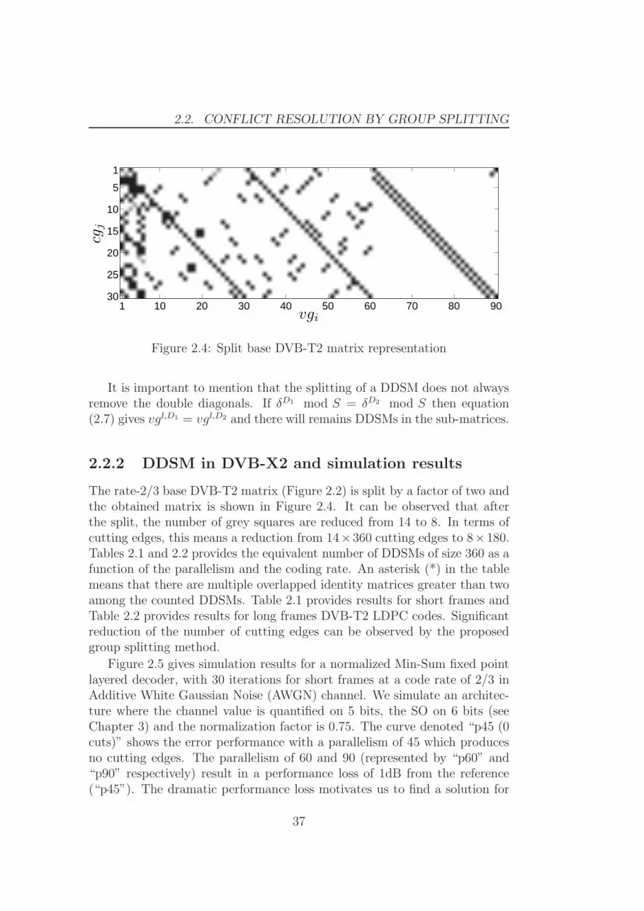
2.2. CONFLICT RESOLUTION BY GROUP SPLITTING
vgi
cgj
10 20 30 40 50 60 70 80 901
5
10
15
20
25
30
1
Figure 2.4: Split base DVB-T2 matrix representation
It is important to mention that the splitting of a DDSM does not alwaysremove the double diagonals. If δD1 mod S = δD2 mod S then equation(2.7) gives vgl,D1 = vgl,D2 and there will remains DDSMs in the sub-matrices.
2.2.2 DDSM in DVB-X2 and simulation results
The rate-2/3 base DVB-T2 matrix (Figure 2.2) is split by a factor of two andthe obtained matrix is shown in Figure 2.4. It can be observed that afterthe split, the number of grey squares are reduced from 14 to 8. In terms ofcutting edges, this means a reduction from 14×360 cutting edges to 8×180.Tables 2.1 and 2.2 provides the equivalent number of DDSMs of size 360 as afunction of the parallelism and the coding rate. An asterisk (*) in the tablemeans that there are multiple overlapped identity matrices greater than twoamong the counted DDSMs. Table 2.1 provides results for short frames andTable 2.2 provides results for long frames DVB-T2 LDPC codes. Significantreduction of the number of cutting edges can be observed by the proposedgroup splitting method.
Figure 2.5 gives simulation results for a normalized Min-Sum fixed pointlayered decoder, with 30 iterations for short frames at a code rate of 2/3 inAdditive White Gaussian Noise (AWGN) channel. We simulate an architec-ture where the channel value is quantified on 5 bits, the SO on 6 bits (seeChapter 3) and the normalization factor is 0.75. The curve denoted “p45 (0cuts)” shows the error performance with a parallelism of 45 which producesno cutting edges. The parallelism of 60 and 90 (represented by “p60” and“p90” respectively) result in a performance loss of 1dB from the reference(“p45”). The dramatic performance loss motivates us to find a solution for
37

CHAPTER 2. MEMORY UPDATE CONFLICTS
Short FrameS Ps 1/4 1/2 3/5 2/3 3/4 4/5 5/6
1 360 4 8 0 14 9 9 20*2 180 1 2 0 4 5 8 13*3 120 1 1 0 3 3 2 114 90 0 1 0 2 2 7 5*5 72 1 1 0 5 1 1 16 60 0 0 0 1 1 2 68 45 0 1 0 0 2 2 4*9 40 1 0 0 1 2 0 310 36 0 0 0 1 0 1 1
Table 2.1: Number of DDSM for N=16200
Long FrameS Ps 1/2 3/5 2/3 3/4 4/5 5/6
1 360 8 32* 12 23* 31* 35*2 180 4 19 5 10 13 213 120 2 16 4 8 15 124 90 2 8 2 3 6 135 72 0 8 2 3 9 116 60 1 6 1 3 5 38 45 0 2 0 3 3 59 40 2 4 1 3 4 210 36 0 4 1 2 2 5
Table 2.2: Number of DDSM for N=64800
38

2.3. PARITY CHECK MATRIX EQUIVALENT
1.5 2 2.5 3 3.5 410
−6
10−5
10−4
10−3
10−2
10−1
100
Eb/N
o(dB)
BE
R
p120 (1080 cuts)p90 (720 cuts)p60 (360 cuts)p45 (0 cut)
Figure 2.5: BER as a function of the parallelism on a fixed point simulation
the remaining DDSMs in the next section.
2.3 Parity check matrix equivalent
In [15] and [56] a method to transform a parity check matrix by the introduc-tion of dummy VN of degree two is presented. With the help of this method,we build an equivalent matrix without DDSMs.
2.3.1 Principle of the split-extend process
Taking into consideration one parity equation (2.9), it can be split-extendedinto two equations (2.10) and (2.11) using a dummy VN p0.
v1 + v2 + v3 + v4 = 0 mod 2 (2.9)
v1 + v2 + v3 + p0 = 0 mod 2 (2.10)
39

CHAPTER 2. MEMORY UPDATE CONFLICTS
Figure 2.6: Principle of an extended parity check matrix
v4 + p0 = 0 mod 2 (2.11)
A dummy VN has an initial LLR value equal to 0. The same splittingprocess can be applied to a layer. In Figure 2.6, a layer (a) with one DDSMis split-extended into two layers (b). The new equivalent matrix is extendedby a a Group of Dummy VN (DG). After the split-extending process, thetwo layers are without DDSM. It is possible to keep the original matrix forthe encoding, which means that there is no change in the architecture ofthe encoder. However, during the decoding process, the added VNs (dummyVN) are initialized with LLR values of 0 and the new matrix is used forthe decoding process. By using the BP algorithm, a flooding schedule andenough iterations, the performance of the extended matrix is equivalent tothe original one. The equivalent matrix is less effective for a layered decoder:the dummy VNs of degree two are used only for the communication betweenthe split CNs. The messages going through the punctured VN are updatedjust one time during one iteration. This means one iteration latency is neededfor the message to be sent from one split CN and received by the other. Thenext subsection presents the results of simulation on a fixed point normalizeddecoder as described in Chapter 3.
2.3.2 Simulation results
Figure 2.7 shows the simulation result keeping the same conditions as inFigure 2.5 but utilizing extended matrices. The values between round bracketrepresent the number of extended sub matrice. Note that the simulationsare with short frame and without the outer BCH decoder. Simulation withstandard frame and BCH correct the error floor and fulfill the standard limit.Simulations with short frame and without BCH have the advantage of faster
40

2.3. PARITY CHECK MATRIX EQUIVALENT
1.5 1.6 1.7 1.8 1.9 2 2.1 2.2 2.3 2.410
−10
10−8
10−6
10−4
10−2
100
Eb/N
o(dB)
BE
R
p360(12EXT)p72(5EXT)p60 (1EXT)p45 (0)Std limit
Figure 2.7: BER as a function of the parallelism with extended matrices
simulation. One can observe the performance degradation with the increaseof the parallelism.
Figure 2.8 shows a simulation for long frames at parallelism of 40 whichis the minimum required parallelism for a 200 MHz pipelined layered decoderto reach the expected 90 Mbps throughput (see Section 4.2). The simulationresults are presented for rates 2/3, 3/4, 4/5 and 5/6. The curves representedby dashed lines are the references at a parallelism that gives no conflict(see Table 2.2). The curve represented by solid lines are the results with aparallelism of 40 and extended matrix. An error floor can be observed forrate 2/3, 3/4 and 4/5 this shows that the proposed solution introduces asignificant degradation of performances.
2.3.3 Performance improvement
To improve the performance, it is important to find first where the errorcomes from, which can be difficult to detect as this error occurs on averageonly once in every 108 bits.
Problem description
Let us analyse what does happen exactly on an example. Figure 2.9 is aTanner representation of the figure 2.6. In this example, V G3 and V G′
3
41

CHAPTER 2. MEMORY UPDATE CONFLICTS
1.5 2 2.5 310
−10
10−8
10−6
10−4
10−2
100
Eb/N
o(dB)
BE
R
referenceextendedstd 2/3std 3/4std 4/5
2/3 3/4 4/5 5/6
Figure 2.8: BER for standard frames with parallelism of 40 with extendedmatrices
Figure 2.9: Tanner representation of Figure 2.6 (b)
42

2.3. PARITY CHECK MATRIX EQUIVALENT
represent the same variable group but they are differentiated in the Tannergraph for better understanding.
Let us follow the message passing evolution of the update of one split CN(The CNs and VNs used during this update are colored in the Tanner graph ofFigure 2.9). At the first sub-iteration it0 and first layer, the Dummy Variable(DV ) get the extrinsic message from V1, V2 and V3. Supposing a min-sumalgorithm and the V3 is a minimum value, then V3 message is transmitted toDV . During processing of the second layer, the V3 message is transmitted toV ′3 through DV . In fact, when the minimum is in V1, V2 or V3, the message
passing works exactly like if the parity check were not split. Supposing nowthat the minimum is in V ′
3 , this minimum is transmitted at the DV onlyduring the second layer processing, and the first layer of it0 does not takebenefit of this message. The first layer will benefit from this message onlyat the next iteration it1. This is where the problem comes from: with thismatrix configuration, there is one iteration delay for the reading of the V ′
3
value. The probability that this delay leads to a mistake is very low, but inpractice, produces the error floor.
Proposed solution
To sum-up, the root of the problem is that DV = V ′3(it− 1) and should be
ideally DV = V ′3(it). If during the read process of layer CG1, we read directly
the V ′3 value instead of the V D value, then we read the last V ′
3 updated valueand the problem is solved. It is not allowed to write two times at the sameaddress during updating of one layer (it will cause overwrite) but it is allowedto read two times at the same address without problem.
Simulation results
Figure 2.10 is a simulation in similar condition as in Figure 2.8 but for shortframes. The simulation results are presented for rates 2/3, 3/4 and 5/6. Thenew curves are less than 0.05 dB from the reference.
Figure 2.11 is a simulation in similar condition as in Figure 2.8. At thedifference of Figure 2.8, the performances are well in the standard require-ments, even without BCH.
The values given in Table 2.1 and 2.2 gives the number DDSM and alsogives the number of DV that have to be added to solve the conflicts. For agiven parallelism, the maximum value of the line multiplied by 360 gives therequired number of DV to add to the architecture as an over cost. The SOmemory over cost is 2.2 % for a parallelism Ps = 40, 3.3 % for Ps = 60, 8.8% for Ps = 120 and 20 % for Ps = 360.
43

CHAPTER 2. MEMORY UPDATE CONFLICTS
1.5 2 2.5 3 3.510
−10
10−8
10−6
10−4
10−2
100
Eb/N
o(dB)
BE
R
referenceextendedstd 2/3std 3/4std 4/5
2/3 3/4 4/5
Figure 2.10: BER for short frames with a parallelism of 40 with extendedmatrices
1.4 1.6 1.8 2 2.2 2.4 2.6 2.8 3 3.2 3.410
−10
10−8
10−6
10−4
10−2
100
Eb/N
o(dB)
BE
R
referenceextendedstd 2/3std 3/4std 4/5
2/3 3/4 4/5 5/6
Figure 2.11: BER for long frames with a parallelism of 40 with extendedmatrices
44

2.4. CONFLICT RESOLUTION BY LAYER DUPLICATION
Another drawback of the solution we proposed comes from a through-put reduction that can become significant in case of high parallelism. Thethroughput is reduced due to the two added identity matrices for each DDSMs.For example, in case of a rate-5/6 short frame with a parallelism of 40,the 3 DDSMs are removed by adding 6 identity matrices. Comparing withthe 2055 identity matrices, this leads to a throughput reduction factor of2055/(2055+6) which is negligible. To have a simple architecture, we choosethe solution to have a constant CN degree (dc). This means that for addedlayer of Dc = 2, null operation are added to have Dc = const. The resultingthroughput is now reduced proportionally to the ratio number of DDSMsover the number of layers. In case of a single stream decoder the proposedsolution is efficient because the required parallelism is low which means afew DDSM to solve. In case of a multi stream decoder (See Section 4.5), therequired throughput is multiplied by the number of streams, which increasethe required parallelism and consequently the number of DDSM. With ahigh number of DDSM, the throughput loss becomes significant and anothersolution has to be considered.
2.4 Conflict Resolution by Layer duplication
The equivalent extended solution is efficient in term of performance but re-duce the decoding throughput. Since the DDSM are solved by the processingof two layers instead of one, the question arises “ can we solve the DDSMand further benefits from the second layer processing?”. Iterative decodingwith replicas [69] shows that it is possible to update a layer two times duringan iteration. The idea is to recall the layers that have DDSM and use a writedisable when needed.
In this section, the split process (see Section 2.2) is kept to reduce thenumber of DDSM and then the layers that include conflicts are now simplyduplicated and the conflicts are solved thanks to an efficient “on time” writedisable of the memory. The advantage is that the added layer solves theDDSM problem, while still taking part in the decoding process.
This section is organized as follows: we first explain the principle of layerduplication and on time write disable. Then we present and solve the problemthat arise in the Mc→v messages. Finally, the architecture and performanceresults are presented.
45

CHAPTER 2. MEMORY UPDATE CONFLICTS
2.4.1 Conflict resolution by Write Disabling the mem-
ory
The principle of conflict resolution by write disabling is to control appropri-ately the writing of the updated SO values when there is a DDSM. Let usrecall first where the memory update conflict comes from (see Section 2.1).In order to facilitate the explanation, we recall equations (2.2) and (2.3).
SOnew1
vdd= SOold
vdd+∆Mc1→vdd (2.12)
SOnew2
vdd= SOold
vdd+∆Mc2→vdd (2.13)
The SOvdd value is updated sequentially two times by equation (2.12) andthen equation (2.13). The result of the layer update is:
SOLR1
vdd= SOold
vdd+∆Mc2→vdd (2.14)
To benefit from the two updates, Equation (2.13) should be:
SOvdd = SOoldvdd
+∆Mc2→vdd +∆Mc1→vdd (2.15)
After a first layer computation, we duplicate the layer, and compute againthis layer. By applying Equation (2.12) to the result of the first layer update(SOLR1
vdd) we obtain Equation (2.15) which is the result we are looking for.
Then normally, the second update apply Equation (2.13) and overwrite theresult were looking for. To overcome this problem, the SO memory is writedisabled during the second update by a write disable, SO is kept unchanged.
In Figure 2.12(a), a sub iteration layer has one DDSM and the SOs areread and written in the same order as they appear in the matrix, from left toright. The result of the diagonal D2 in the DDSM will overwrite the resultof the diagonal D1 (D1 in dash line shows the overwrite). Figure 2.12 (b)and (c) is an example where the layer labeled LR1 is the first occurrenceand LR2 is the second occurrence. During the first layer, the result fromthe left diagonal (D1) is overwritten but the result of the right diagonal(D2) is updated. During the second layer occurrence, a write disable signalis generated to disable D2 update. This time, the result of D1 is updated.With the recall process associated with an on time write disable, the memoryoverwrite still occurs but it is corrected thanks to the layer duplication.
2.4.2 Scheduling of the layers
The suspension points between Figure 2.12 (b) and (c) indicate layers be-tween LR1 and LR2. These layers are included to avoid memory conflicts due
46

2.4. CONFLICT RESOLUTION BY LAYER DUPLICATION
WD+
Repeat layer
WD
OverwriteOverwrite
...Overwrite
Write Disable
Layer Repeat 1
Layer Repeat 2
Overwrite
(b)
(c)
(a) No layer repeat
Result
SOLDD,D2vdd
= SOoldvdd
+∆Mc2→vdd
LR2
LDD
D1 D2
SOnewvdd
= SOoldvdd
+∆Mc1→vdd +∆Mc2→vdd
SOLR1,D1vdd
= SOoldvdd
+∆Mc1→vdd
SOLR1,D2vdd
= SOoldvdd
+∆Mc2→vdd
LR1
D1 D2
SOLR2,D1vdd
= SOLR1,D2vdd
+∆Mc1→vdd
SOLR2,D2vdd
= SOLR1,D2vdd
+∆Mc2→vdd
SOLdd,D1vdd
= SOoldvdd
+∆Mc1→vdd
Figure 2.12: repeat layer principle
47

CHAPTER 2. MEMORY UPDATE CONFLICTS
to pipeline [46] between LR1 and LR2. Furthermore, because LR1 and LR2
use the same SO values, if LR2 would be just after LR1 the result of LR2 isidentical to LR1 and there is no progress in the iterative process. If betweenLR1 and LR2, the SO values are updated, then LR2 benefits from these newupdated values. In order to benefit from more updated SO values, an ef-ficient scheduling of the layers would include a maximum number of layersbetween LR1 and LR2. During the next iteration, in order for LR1 to benefitfrom LR2 updating, LR2 and LR1 should also include a maximum number oflayers. Ideally, LR1 and LR2 should be separate by half the number of layers.
This repeat layer principle is quite simple. Nevertheless while the SOMemory is write disabled, the Mc→v is still updated which will lead to errors.In terms of hardware implementation, specific mechanisms are required inorder to keep coherence between Mc→v memory and SO memory.
2.4.3 Write disabling in the Mc→v memory
During one sub iteration with one DDSM, from equations (2.12) and (2.13),the SOnew2
v will overwrite the SOnew1v value. The edge of the Tanner graph
connecting c1 to vdd is virtually absent in the decoding process. Nevertheless,at the next iteration from (1.15), the Mv→c1 is given by:
M itvdd→c1
= SOv −Moldc1→vdd
(2.16)
The edge c1 → vdd has been cut during the previous iteration, this meansthat Mold
c1→vddshould not provide the Mnew
c1→vddvalue computed during the
previous iteration. A possible implementation is to Write Disable (WD) theMMEM
c→v memory when storing Mnewc1→vdd . This process keeps Mc→v at address
of diagonal one (D1) in the Mc→v memory at the previous value.Let us now focus on the DDSMs in the repeated layers in Fig 2.12 (b)
and (c). During the LR1 (b) computation, the Mc→v memory at address (D1)is write disabled and during the LR2 (c) computation, the Mc→v memory ataddress (D1) is write disabled.
Write disable algorithm
There is a need for an on time WD of the SO memory and the Mc→v memoryin function of the layer occurrence (LR1 and LR2) and the diagonal numberin the DDSM (D1 and D2). This is summed-up in Algorithm 1.
This algorithm is efficient for no compressed Mc→v memory where eachedge has an address in the memory. In case of a min-sum algorithm, there isno more access toD1 andD2 because all the edges of one layer are compressedand stored in one address. This problem is solved in the next subsection.
48
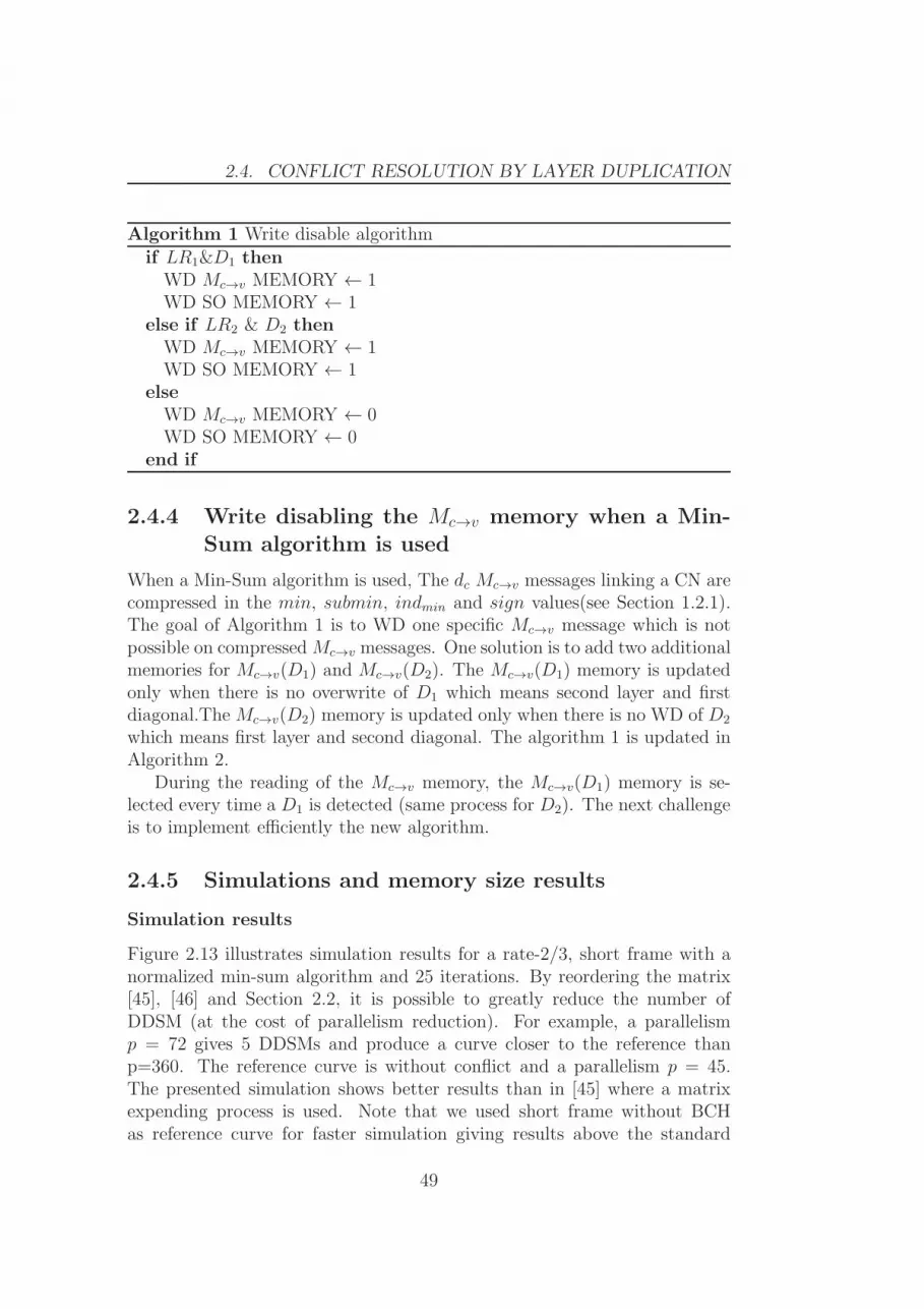
2.4. CONFLICT RESOLUTION BY LAYER DUPLICATION
Algorithm 1 Write disable algorithm
if LR1&D1 thenWD Mc→v MEMORY ← 1WD SO MEMORY ← 1
else if LR2 & D2 thenWD Mc→v MEMORY ← 1WD SO MEMORY ← 1
elseWD Mc→v MEMORY ← 0WD SO MEMORY ← 0
end if
2.4.4 Write disabling the Mc→v memory when a Min-Sum algorithm is used
When a Min-Sum algorithm is used, The dc Mc→v messages linking a CN arecompressed in the min, submin, indmin and sign values(see Section 1.2.1).The goal of Algorithm 1 is to WD one specific Mc→v message which is notpossible on compressed Mc→v messages. One solution is to add two additionalmemories for Mc→v(D1) and Mc→v(D2). The Mc→v(D1) memory is updatedonly when there is no overwrite of D1 which means second layer and firstdiagonal.The Mc→v(D2) memory is updated only when there is no WD of D2
which means first layer and second diagonal. The algorithm 1 is updated inAlgorithm 2.
During the reading of the Mc→v memory, the Mc→v(D1) memory is se-lected every time a D1 is detected (same process for D2). The next challengeis to implement efficiently the new algorithm.
2.4.5 Simulations and memory size results
Simulation results
Figure 2.13 illustrates simulation results for a rate-2/3, short frame with anormalized min-sum algorithm and 25 iterations. By reordering the matrix[45], [46] and Section 2.2, it is possible to greatly reduce the number ofDDSM (at the cost of parallelism reduction). For example, a parallelismp = 72 gives 5 DDSMs and produce a curve closer to the reference thanp=360. The reference curve is without conflict and a parallelism p = 45.The presented simulation shows better results than in [45] where a matrixexpending process is used. Note that we used short frame without BCHas reference curve for faster simulation giving results above the standard
49

CHAPTER 2. MEMORY UPDATE CONFLICTS
Algorithm 2 Write disable algorithm for min-sum
if Layer = LR1 then
if D1 thenWD SO MEMORY ← 1
else if D2 thenWE Mc→v(D2) MEMORY ← 1
end ifelse if Layer = LR2 then
if D1 thenWE Mc→v(D1) MEMORY ← 1
else if D2 thenWD SO MEMORY ← 1
end ifelseWD SO MEMORY ← 0WE Mc→v(D2) MEMORY ← 0WE Mc→v(D1) MEMORY ← 0
end if
requirement. If standard frame and BCH were used, the performance wouldbe in the standard requirements.
To compare the curve at a constant throughput, in Figure 2.14 the num-ber of iteration is reduced in function of the number of added layers. Thereference curve is without conflict and 30 iterations. With a parallelism of120 (3 DDSM), 3 layers are repeated over the 15 layers. To keep a constantthroughput, the number of iterations is reduced by a factor 15/(15 + 3),which gives 25 iterations. With a parallelism of 360 (14 DDSM), the numberof iteration is reduced by 15/(15+14) which gives 16 iterations and the curveis at only 0.1 dB away from the reference.
Memory size
When using compressed Mc→v memory, there is a need to store the Mc→v
values for every DDSM. The Memory over cost in bits is equal to two timesthe Mc→v word size times the number of DDSM times the parallelism P . Incase of a parallelism of 360 the memory over cost becomes significant i.e. 126Kbits for long frame and rate 5/6.
When using a not compressed Mc→v memory, there is no more need of
50
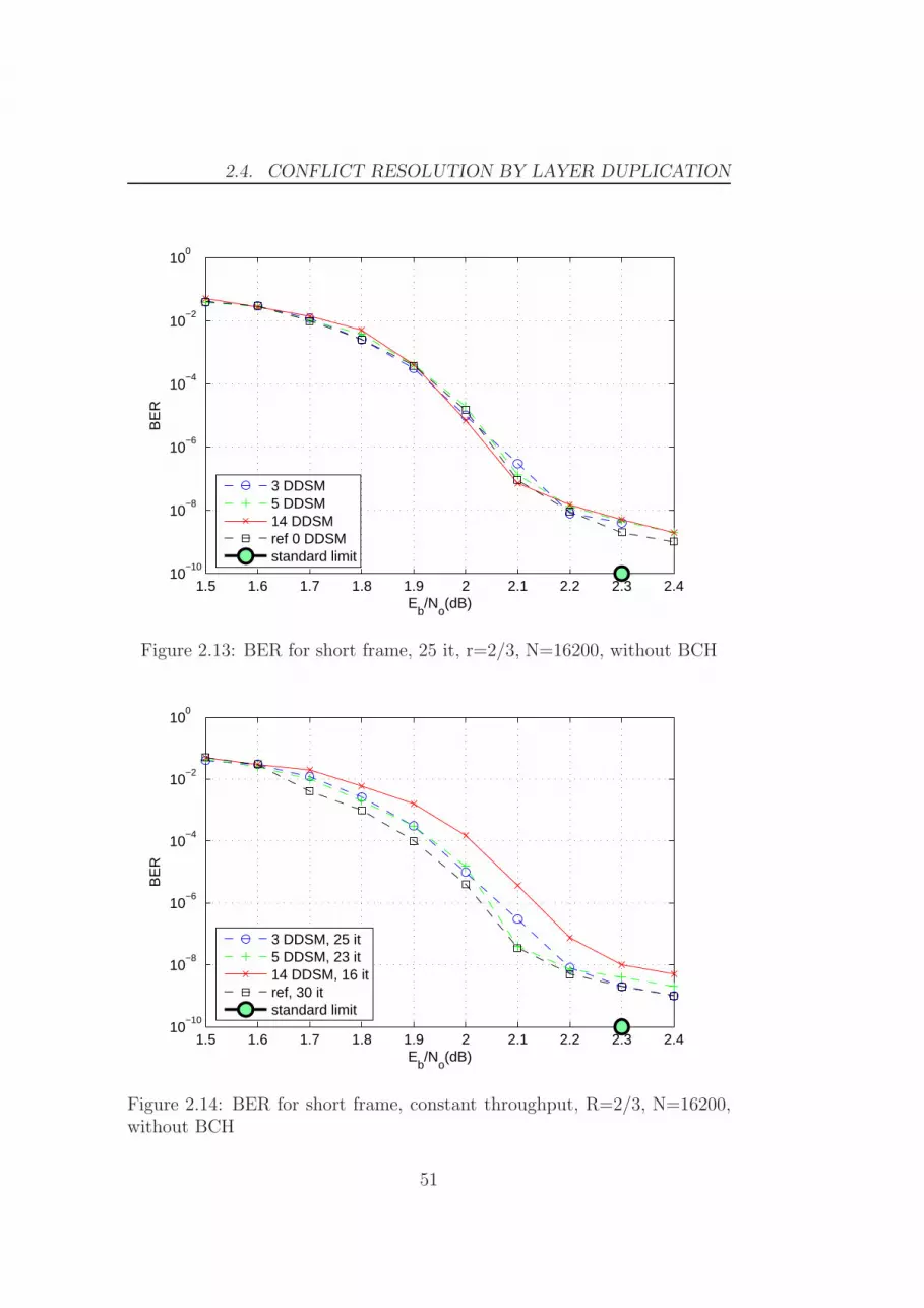
2.4. CONFLICT RESOLUTION BY LAYER DUPLICATION
1.5 1.6 1.7 1.8 1.9 2 2.1 2.2 2.3 2.410
−10
10−8
10−6
10−4
10−2
100
Eb/N
o(dB)
BE
R
3 DDSM5 DDSM14 DDSMref 0 DDSMstandard limit
Figure 2.13: BER for short frame, 25 it, r=2/3, N=16200, without BCH
1.5 1.6 1.7 1.8 1.9 2 2.1 2.2 2.3 2.410
−10
10−8
10−6
10−4
10−2
100
Eb/N
o(dB)
BE
R
3 DDSM, 25 it5 DDSM, 23 it14 DDSM, 16 itref, 30 itstandard limit
Figure 2.14: BER for short frame, constant throughput, R=2/3, N=16200,without BCH
51

CHAPTER 2. MEMORY UPDATE CONFLICTS
SignT
+
+
−RAM_SO
Bar
el S
hifte
r
VGnVGn2
GeneratorIndex
Min_1
Min_0
Sign
RA
M(M
/P)
WE_SO
FIFO(Dc)
SortingSerial
XOR
Serial
generator
Check node core
FIFO(#DD)
FIFO(#DD)
DD
∆Shift
2′s→
SM
SerialMc→v
SM
→2′s
|Mc→v|
SM
→2′s
MV →C
MMEMc→v (D1)
MMEMc→v (D2)
DD1
MC→V memory
WE DD1
WE DD2DD2
Figure 2.15: write disable architecture
adding specific memory. Considering the memory size optimization describedin [44] and in Chapter 3, a compressed version requires 875 Kbits and a noncompressed version requires 1100 Kbits. Adding 126 Kbits on the compressedside, the non compressed solution still leads to a 10 % memory over cost butgives alternative to the Min-Sum algorithm. An alternative to Min-Sumalgorithm can be interesting to improve performance and to solve the errorfloor problem for the low code rates.
2.4.6 The write-disable architecture
In this subsection, we describe the three main modifications added to thelayered decoder architecture 1.3.4 to implement the WD algorithm.
Layer duplicating
In the architecture overview (see Section 1.3.4, the Mc→v memory can bemade of a FIFO memory as a Mc→v update occurs only once during oneiteration. In case of repeated layers, the Mc→v are updated more that onceand the Mc→v read and write must be at the same address as during thefirst call. This can be implemented using a RAM and an ad hoc addressgenerator. From the counter and the ROMdc, the layer number signal isgiven. The ROMMcv gives a constant address when a layer is repeated.
52

2.4. CONFLICT RESOLUTION BY LAYER DUPLICATION
XQ5VLX85 LUT LUT RAM BRAM
Node Processor 143 2 0sorting 37 0 0
gen mc→v 34 0 0fifo mv→c 12 2 0
mc→v memory 46 0 3Total 1 node 189 2 3Total 45 nodes 8586 90 135
Control 667 3 0
block SO RAM 360 0 22
Channel RAM 48 0 25
Barrel shifter 945 0 0
Total 11005 93 182
Percentage [%] 5 1 50
Table 2.3: Synthesis Results for DVB-S2 LDPC decoder
Cutting edge and repeat layer detection
The cutting-edge detector principle relays on the detection of DDSM. Whenthere is a DDSM, during the serial read of the VNGs, two equal V NGn valuesfollows. This can be easily detected at the output of ROMV NGn where thebase matrix is stored. A repeat layer detector is implemented by using adedicated ROM. In this ROM, for each layer is stored if the layer is a repeatlayer and if the layer is the first or the second occurrence.
Knowing the status of a layer (normal, LR1 or LR2) and the status of anIM (normal, D1 or D2), it is possible deducted from the Algorithm 2 thestates of the WD signals (WDSO , WE D1 and WE D2)
2.4.7 Synthesis results on FPGA
The architecture presented in Figure 2.15 with finite precision options de-scribed in Section 3 was synthesized on a Virtex-V Pro FPGA (XQ5VLX110)from Xilinx, for validation purposes. The system decodes long frames of coderate 2/3. Table 2.3 reports the hardware resources required. The clock fre-quency is 200 MHz, the average number of iterations is 20 and the throughputis 90 Mbit/s, which allows the decoding of two simultaneous High-DefinitionTelevision (HDTV) streams.
53

CHAPTER 2. MEMORY UPDATE CONFLICTS
2.4.8 Conclusion
To deal with the memory conflict problem, we proposed a solution based onrepeating the layers with DDSM. The repeating process is associated withan efficient write disable of the memory to overcome the conflict problem.This technique shows in worst case performance at 0.1db from the referencewithout throughput loss. The implementation area benefits from the use ofonly one barrel shifter and a simple memory access at the price of a slightmemory increase and control over cost. This technique shows, in worst case,performance at 0.1db from the reference without throughput loss. The nextstep is to solve the conflicts due to the pipelining.
2.5 Memory update conflicts due to pipeline
Many of the current LDPC implementations of DVB-X2 or WiMAX [60]standard use the so-called layered architecture combined with pipeline [62,54, 14, 57]. However, the pipeline process may introduce memory updateconflicts.
In [53] and [8] the authors present a solution based on the computation ofthe variation (or delta) of the SO metrics to allow concurrent updates. Thecomputation of this SO update (SOnew = SOold + delta) is efficient to solvethis kind of conflict but needs either a costly additional memory access or anincrease in the clock frequency by a factor of two. In [62], the use of idle timeis proposed to deal with the conflicts. However this solution decreases thethroughput. The scheduling of the SO in [54] reduced the use of idle timeby using CNP able to deliver its outputs values in a different order than itsinput values, which increase the complexity of the CNP architecture. Finally,we should also note that [14], [54] propose an appropriate scheduling of thecheck node as a solution to avoid pipeline conflict but in none of them, theidea is fully developed.
In this section, we focus on the conflicts due to the pipelining of a layereddecoder and we propose solutions with an example on the DVB-T2 matrices.In a first step the splitting process (see Section 2.2) solve by itself a partof the pipeline conflicts. In order to find an efficient scheduling to solve theremaining conflict, we show that the research of an efficient scheduling isequivalent to the well known ”Traveling Salesman Problem”. Thus, all thenumerous methods described in the literature to solve the former problemcan be used for our scheduling problem. In this section, we present schedulingresults using a genetic algorithm.
54

2.5. MEMORY UPDATE CONFLICTS DUE TO PIPELINE
dc
SO
SOnew
ǫ
Figure 2.16: Chronogram of a non pipelined CNP
2.5.1 Non pipelined CNP
The chronogram in Figure 2.16 illustrates a non-pipelined CNP. The CNPfirst reads the SO. Then after a given number of clock cycles ǫ, i.e. the CNPlatency, the CNP writes back the result of the calculation. We can see onthis chronogram that the CNP starts to read the new set of variable nodesvci+1
only when all the previous vci have been calculated. The correspondingthroughput is given by:
D1 =K.Fclk
(2dc + ǫ).MP.Nit
bit.s−1 (2.17)
where Nit is the number of iterations to decode a codeword, M is the numberof CN, P is the number of CNPs working in parallel, dc is the average numberof VNs linked to a CN, Fclk is the clock frequency and K is the number ofinformation bits in a codeword.
2.5.2 Pipelined CNP
Pipelining allows a more efficient use of the CNP and an increase of thethroughput [62], [4] and [54]. The pipelining consists in reading the vci of onesub-iteration while writing on vci−1
the result of the previous sub-iteration.This means that as soon as the reading of one sub-iteration is finished, a newone is started. The chronogram is given in Figure 2.17 and the correspondingthroughput is given by the following equation:
D2 =K.FClk
dc.MP.Nit + dc + ǫ
bit.s−1 (2.18)
The pipelined architecture offers at least two times greater throughputcompared to the non pipelined one: D2
D1≈ 2 + ǫ
dc. We will see in the next
subsection that this architecture can lead to memory conflicts.
55

CHAPTER 2. MEMORY UPDATE CONFLICTS
dc
SOnew
SO
ǫ
Figure 2.17: Chronogram of a pipelined CNP without idle time
2.5.3 The problem of memory update conflicts
In this subsection, we describe the memory update conflicts and we differen-tiate two types of conflicts.
”Type i+ 1” memory conflict: In Figure 2.17 a common variable SOcom
(filled square) is used in two successive sub-iterations. During the second sub-iteration, the SOcom is still not updated from the previous sub-iteration andthe result of the current sub-iteration will overwrite the result of the previoussub-iteration. This is also known as a ’cutting edge’ problem because it isequivalent to a cut in an edge of the Tanner graph representation of thematrix. Let vgcgi be the set of all the vgi connected to cgj. During pipelining,the P CNPs write on vgcgi while the P CNPs read on vgcgj . The layers cgiand cgj can work one after the other without memory access conflict whenthe two groups don’t share any common variable 1. Mathematically speaking,this constraint can be expressed by:
vgcgi ∩ vgcgj = ∅
For example, we can check in Figure 2.2 that there is no vgi in commonbetween the set of vgi linked to the group of check node number one cg1 andeleven cg11:
{vgcg1} ∩ {vgcg11} ={1,2,12,16,19,24,31,45}∩{3,11,13,15,17,21,26,40,41}=∅
Thus the decoding of cg1 and cg11 can be processed consecutively withoutmemory update conflict. To avoid memory update conflicts, we have to takecare that at any time, two sub-iterations does not share any SO in common.
1As mentioned in [54], if dc > ǫ, it is still possible to avoid memory conflict betweentwo groups sharing the same common variable SOcom by an appropriate scheduling of theSOcom inside the two consecutive layers.
56

2.5. MEMORY UPDATE CONFLICTS DUE TO PIPELINE
SO
dc
ǫSOnew
Figure 2.18: Conflict due to pipelining at i+ 2
”Type i+ 2” memory conflict: Figure 2.18 illustrates that the same con-sideration must be taken with the i+ 2 sub-iteration because of the latencyǫ. In this figure, one value of SO generated by layer i is written in memoryafter it is read by layer i+ 2. This situation also leads to a memory conflictand can be avoided by appropriate scheduling of the layers.
2.5.4 Conflict reduction by group splitting
Section 2.2 explaines how to split an identity matrix in multiple sub-identitymatrices. This process was used to reduce the number of memory updateconflicts due to the structure (Section 2.1). Again, the split process is usedto solve memory update conflict but the causes and the reasons are different.
The Figure 2.4 illustrates the new base matrix after splitting by a factorof 2. We can see that the new base matrix is sparser than the base matrixin Figure 2.2 (in terms of identity matrix density). In fact, the number ofidentity matrices increases by 2 while the size of the base matrix is increasedby 2 × 2. Increasing the split decreases the risk of memory conflicts due topipelining. An appropriate scheduling of the layers can solve the remainingconflicts.
2.5.5 Conflict resolution by scheduling
A schedule provides timing information about a series of arranged events. Toavoid the cutting edge conflict, we explore the scheduling of the layers. Afterdefining the scheduling strategy, we show that this problem is an instanceof the well known ”Traveling Salesman Problem”. This problem can beefficiently solved by a Genetic Algorithm (GA).
57

CHAPTER 2. MEMORY UPDATE CONFLICTS
Scheduling of the layers
The schedule is done in the set of groups of CNs cg = {cg1, cg2, ..., cgmg}.We define a schedule sequence index π, where π is one permutation in theset {1, 2, ..., mg}. The number of conflicts due to the pipelining between twocheck node groups cgi and cgj is given by equation (2.19).
c(i, j) = |vgcgi ∩ vgcgj | (2.19)
The number of conflicts after one full iteration using scheduling π is givenby equation (2.20).
cit(π) =
(
i=mg−1∑
i=1
c(π(i), π(i+ 1))
)
+ c(π(mg), π(1)) (2.20)
where the second term is the cost between the last layer of an iterationand the first layer of the following iteration. We have to find the optimalpermutation πopt that gives the smallest number of conflicts. This can betranslated into an optimization problem which consists in the minimizationof the cost function:
πopt = argmin{cit(π), π ∈ Π} (2.21)
where Π is the group of all the possible permutations of π. The use of graphtheory is dedicated to solve this kind of problem.
The Traveling Salesman Problem (TPS)
Finding the schedule to avoid cutting edge is described by the minimizationproblem (2.21). An equivalent formulation in terms of graph theory is: givena complete weighted graph (where the node would represent a group of CNs,and the number of cutting edge would be the cost of the edge), find a Hamil-tonian cycle with the least cost. An Hamiltonian cycle consist in visitingeach node exactly once and also return to the starting node. This problem isalso known as a TSP [38]. The TSP statement is as follows: given a numberof cities and the cost of traveling from one city to any other city, what isthe least-cost round-trip route that visits each city exactly once and thenreturns to the starting city. In our case a town is a group of check node andthe traveling cost is the number of cutting edges (2.19).
The first step is to build the cost matrix Hc = {Hc(i, j) = c(i, j), i, j ∈[1, mg]2}. This matrix gives the number of cutting edges for each possiblecouple of groups of CN cgi and cgj . The cost matrix for a rate 2/3 shortframe is illustrated in Figure 2.19(a). On this graphical representation, a
58

2.5. MEMORY UPDATE CONFLICTS DUE TO PIPELINE
CGi
CG
j
5 10 15
2
4
6
8
10
12
14
(a) Without split
CGi
CG
j
10 20 30
5
10
15
20
25
30
(b) With a split factor of 2
Figure 2.19: Cost matrix
white square is for no cutting edge and a grey square means one (light grey)or more (darker grey) cutting edges.
We can see in Figure 2.19(a) that there are only three couples cg1,11 , cg8,14and cg10,14 that can perform consecutively without conflicts. Figure 2.19(b)shows the cost matrix after a split factor of 2. The new matrix offers morepossible couples without memory conflict (from 3% to 20% after splittingby two). The split process gives fewer cutting edges and a greater degree offreedom for scheduling.
The problem of trying all permutations (|Pi| = mg!) and selecting theminimum cost (2.21) is NP hard in O(mg!). For a long frame of rate 1/4and split 4, the number of cities are 540. Thus a suboptimal or heuristicalgorithm is needed to solve the problem.
Principle of Genetic Algorithm
Genetic algorithms [32, 38] use techniques inspired by evolutionary biologysuch as inheritance, mutation, selection and crossover. The genetic algorithmprocess is summarized in Figure 2.20. First, many solutions are randomlygenerated to form an initial population. Then individual solutions are se-lected through a two round tournament selection using the fitness functiongiven by equation (2.20). The next step is to generate the ’children’ througha two point crossover between solutions previously selected. The last step isthe mutation of the children for diversity purpose by swapping two randomly
59

CHAPTER 2. MEMORY UPDATE CONFLICTS
2.Fitness Test
+ =
4.Crossover
1.Initial Populaion
+?=
6.Mutation
5.Children3.Select Best Parents
One generation
7.New population
=?
Figure 2.20: Genetic algorithm
chosen cities. This generational process is repeated until a null cost is foundfor an individual solution or a fixed number of generations is reached.
The result of the genetic algorithm applied to the scheduling problem ispresented in the next section.
Simulation results
In this section, we present the result of the genetic algorithm. The maximumnumber of generation and the initial population were set to 1000. Every so-lution was obtained in less than 15 minutes on a standard desktop processingunit.
In order to take into account the ”type i + 2” cutting edge defined insection II.D, i.e vgcgi ∩ vgcgi+2
= ∅, we modify the cost function cit defined in(2.20) as:
c′it(π) = αcit(π) +
mg∑
i=1
c(π(i), π((i+ 2) mod mg)) (2.22)
where α ∈ N+ and is high enough to give an absolute priority to the i + 1conflicts against the i + 2 conflicts. The next subsection gives some resultsusing a genetic algorithm to find an efficient schedule.
Table 2.4 and Table 2.5 present the results found for the DVB-T2 LDPCdecoder. In these tables, a ’0’ means that the genetic algorithm found no
60

2.5. MEMORY UPDATE CONFLICTS DUE TO PIPELINE
Code rateS Ps 1/4 1/2 3/5 2/3 3/4 4/5 5/6
1 360 1 1 0 0 0 0 02 180 2 2 1 0 1 0 03 120 2 2 1 1 1 1 04 90 2 2 1 1 1 2 15 72 2 2 1 1 2 2 16 60 2 2 2 2 2 2 18 45 2 2 2 2 2 2 19 40 2 2 2 2 2 2 2
Table 2.4: Scheduling solutions for short frames
Code rateS Ps 1/2 3/5 2/3 3/4 4/5 5/6
1 360 2 1 1 1 0 02 180 2 1 2 1 1 03 120 2 1 2 2 1 14 90 2 1 2 2 1 15 72 2 1 2 2 1 16 60 2 2 2 2 2 18 45 2 2 2 2 2 29 40 2 2 2 2 2 2
Table 2.5: Scheduling solutions for long frames
solution that avoids ”type i+1” conflict. A ’1’ (respectively ’2’) means that itfound a scheduling solution without type i+ 1 conflict (respectively withouttype i + 1 and type i + 2 conflicts). We can check that for Ps = 40, thereare schedules without conflicts at i + 2 for all code rates and frame types.Note that, after a scheduling at i + 1, the remaining conflicts due to thelatency ǫ can be avoided using a scheduling of the vgi inside the layers [54].This option allows a parallelism of up to 120 for long frames and 90 for shortframes.
Scheduling of the identity matrices
During the sorting process of the min-sum algorithm in equation (1.8), thearriving order of the VG have no incidence in the result, so it is possible
61

CHAPTER 2. MEMORY UPDATE CONFLICTS
to reorder the VG in a layer without consequences. Table 2.4 and Table 2.5show that for high parallelism there is no layer scheduling that solve equation2.20 (type i+ 1 conflict). Even if two successive layers have a common VG,a conflict doesn’t necessary occurs as in figure 2.17. In the figure 2.17, ifthe common VG (colored square) of the first layer is read at the start of thelayer, and the common VG is at the end of the second layer, then no conflictoccurs. To generalize, if ǫ < dc − 1 then a solution exist by reordering theIM in the layers. If ǫ > dc− 2 then there is no solution for type i+1 conflictand idle time have to be added to the reordering of the IM to avoid conflict.Moreover, if ǫ > dc− 2, then there are possibility of conflict between a layeri and layer i + 2 as in Figure 2.18 (type i + 2 conflict), this conflict can besolved by identity matrix scheduling.
2.5.6 Conclusion
Pipelining a layered decoder doubles the throughput but leads to memoryconflicts. The split process reduces the parallelism and creates sparser basematrices. Using the new base matrices, schedules without conflicts can befound. Due to the huge amount of combinations, a genetic algorithm is usedto find the best schedule. This algorithm finds schedules that avoid conflictswith the next sub-iteration (i + 1) and with the second next sub-iteration(i + 2). Combined with a scheduling of the identity matrices in the layers,the whole scheduling process is able to solve all conflicts due to pipeline. Theproposed solution only requires an efficient scheduling and requires no changeor added patch to the layered architecture. Although this section explainsthe process for matrices defined by the DVB-T2 standard, the same processcan be used for structured matrices such as the ones defined by the WiMAXstandard.
2.6 Combining layers duplication and schedul-
ing
Section 2.4 solves efficiently memory conflict due to the matrices structure.Section 2.5 solves efficiently memory conflicts due to the pipelining. Can wecombine the two methods to solve all the memory update conflicts? Thesplit process explained in Section 2.2 is a common tool as a first step forthe resolution of the two causes of conflicts. The split conflict is compatiblewith the two methods. Then in a second step, the resolution of pipe conflictis solved by minimizing the cost of an Hamiltonian cycle (process all the
62

2.7. CONCLUSION
layers only once during an iteration and return to the starting layer). Thesecond step to solve conflicts due to the structure is to duplicate layers. Theconsequence is that the iteration cycle is not any more Hamiltonian becauselayers are repeated during one iteration. Thanks to the flexibility of theGenetic Algorithm (GA) used to solve the scheduling problem, the data ofthe problem has just to be updated with new layers (the duplicated layers)without any changes in the GA algorithm.
2.7 Conclusion
In this chapter we considered the problem of memory update conflicts due tothe DVB-S2, -T2 and -C2 matrices structure and conflicts due to the use ofa pipelined layered decoder. Conflicts due to the structure has been solvedthank to two innovative solutions and Conflicts due to pipeline has beensolved by an efficient scheduling of the layers. The split procees associatedwith a layer repeat architecture and an efficient layer scheduling can be effi-ciently combined for a memory update conflict free solution. Now that thememory conflict problems are solved, it is possible to think on reducing theimplementation cost by optimizing the architecture.
63

CHAPTER 2. MEMORY UPDATE CONFLICTS
64

If you want a thing done well,
do it yourself.
Napoleon Bonaparte(1769-1821)
3Memory optimization
Summary :In this chapter, the optimization of the memory size is studied. The
DVB-S2 standard is considered to compare results with the literature. Ourwork can also be applied to the DVB-T2 and -C2 standard, the Wi-Fi andWiMAX LDPC standards or more generally to any layered LDPC decoder.The first step concerning the memory reduction is the choice of a sub-optimalalgorithm. The already well-known Min-Sum algorithm [24] and its variantssignificantly reduce the memory needs by the compression of the extrinsicmessages. Another way to reduce the memory needs is to limit the word sizeby saturation. In the state-of-the-art, the way the SO and the extrinsic mes-sages are saturated is rarely explicitly explained. In this chapter, we providefirst some discussion on efficient saturation of the extrinsic messages andthe SO values. To complete the discussion, we also introduce a methodologyto optimize the size of the extrinsic memory. In a second step, still is thefield of memory optimization, as Dual port RAM is much more costly thanSingle port RAM, methodologies are given to implement the layered decoderby using only single port RAM.
65
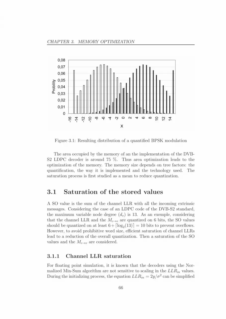
CHAPTER 3. MEMORY OPTIMIZATION
Figure 3.1: Resulting distribution of a quantified BPSK modulation
The area occupied by the memory of an the implementation of the DVB-S2 LDPC decoder is around 75 %. Thus area optimization leads to theoptimization of the memory. The memory size depends on tree factors: thequantification, the way it is implemented and the technology used. Thesaturation process is first studied as a mean to reduce quantization.
3.1 Saturation of the stored values
A SO value is the sum of the channel LLR with all the incoming extrinsicmessages. Considering the case of an LDPC code of the DVB-S2 standard,the maximum variable node degree (dv) is 13. As an exemple, consideringthat the channel LLR and the Mc→v are quantized on 6 bits, the SO valuesshould be quantized on at least 6+⌈log2(13)⌉ = 10 bits to prevent overflows.However, to avoid prohibitive word size, efficient saturation of channel LLRslead to a reduction of the overall quantization. Then a saturation of the SOvalues and the Mc→v are considered.
3.1.1 Channel LLR saturation
For floating point simulation, it is known that the decoders using the Nor-malized Min-Sum algorithm are not sensitive to scaling in the LLRin values.During the initializing process, the equation LLRin = 2y/σ2 can be simplified
66

3.1. SATURATION OF THE STORED VALUES
to LLRin = y, saving the need to compute the variance.The received y valueis quantized in a way to have integer values at the input of the decoder. Weassume here that the quantized value of y denoted by LLRq is representedon nLLR bits and the quantification function is defined as:
LLR(y)q =
⌊
sat(y, R)× 2nLLR−1 − 1
R+ 0.5
⌋
, (3.1)
where sat(a, b) = a if a belongs to [−b, b] and sat(a, b) = sign(a)×b otherwise.The R value is the interval range of quantization ( y is quantized between[−R,R]) and represent also the saturation threshold value. Considering theBPSK modulation, we saturate y at R = 1 + β.
Figure B.3 shows the Probability Density Function of a quantized BPSKmodulation (-1 and +1) that is perturbed by an Additive White GaussianNoise (AWGN) of variance σ = 0.866 (corresponding to Eb/No = 2 dB).The channel is quantized on 5 bits and the saturation threshold is R =1 + β = 2, 47. The distribution filled in black shows the +1 offset, and theunfilled distribution is the -1 offset. The quantized distribution varies fromLLRmin
q = −(24 − 1) to LLRmaxq = 24 − 1. The problematic is to find the
saturation threshold providing the best performance for for a given number ofbits of quantization. If the saturation threshold is low, then the informationgiven by the tail of the Gaussian curve are saturated. If the threshold is highthen the quantization error increases.
The saturation limit 1 + β can be calculated so that the proportion ofsaturated values is equal to the average proportion of the other values. Theaverage proportion of a given value is 1/(2nLLR − 1)(probability of a valuein an uniform distribution). On the other side of the equality, the CumulateDistributive Function (CDF) of a -1 offset distribution applied to the negativesaturation limit will give the proportion of saturated values for a -1 offsetsignal. The equality can be written as:
1
2
[
1 + erf( −β√
2σ
)
]
=1
2nLLR − 1(3.2)
From equation (3.2), β can be deduced:
β = σ ×√2
(
erf−1(2nLLR − 1
2nLLR + 1
)
)
(3.3)
Thus the β value is a function of nLLR and is proportional to σ. Byapplying equations (3.3) and (3.1), the optimum saturation threshold andthe scaling factor can be computed. The problem of this solution is that an
67

CHAPTER 3. MEMORY OPTIMIZATION
1.6 1.7 1.8 1.9 2 2.1 2.2 2.3 2.4 2.510
−10
10−8
10−6
10−4
10−2
100
Eb/N
o(dB)
BE
R
3−8−44−9−55−10−66−11−7Std limit
Figure 3.2: BER simulation for a rate 2/3
adaptative quantization of y is needed that requires a channel estimation ofσ .
In fact, to prevent the σ computation, an optimal scaling factor is calcu-lated for a given SNR. If the performance requirement is reached for a givenSNR, then for higher SNR, the quantization would be sub-optimal. However,even with sub-optimal quantization, with higher SNR, the performance arestill improving. For each code rate, a constant scaling factor ω and saturationvalue 1 + β can be pre-computed saving the need for the σ value.
Effects of LLRin saturation on BER performance
Fig. 3.2 shows the simulation results for a normalized Min-Sum fixed pointlayered decoder, with a maximum of 30 iterations, long frame, code rates2/3 in Additive White Gaussian Noise channel. The normalization factor is0.75. Let us consider the following notation: a 3-8-4 configuration refers toa channel LLR quantized on 3 bits, an SO value word size of 8 bits and aMc→v word size of 4 bits. We also depicted the standard limit at 1 dB fromthe Shannon limit in Eb/N0 for code rate 2/3.
The quantification values of the Mc→v and SO are not optimized andchosen large enough to not affect the results of the channel quantification.Fig. 3.2 shows that a quantification on 4 or 5 bit of the LLRin is enough tofulfill the standard requirements.
68

3.1. SATURATION OF THE STORED VALUES
3.1.2 SO saturation
Once the LLRin quantized, they are stored in an SO memory wich willevoluate with the iteration process. This SO memory need to be saturatedto limit their size
The problem of SO saturation
We first consider the saturation case where SOmax < SOnewv during the SO
update (1.18). The saturation process will bound SOnewv to the SOmax value.
This will introduce an error ǫv in the SOnewv value (ǫ = SOnew
v − SOmax).During the next iteration, the newM ′
v→c value will beM′v→c = SOv−Mc→v =
Mv→c − ǫv.We now consider the worst case: during an iteration, SOv is saturated at
+SOmax, each CN confirms a positive Mc→v value, and dv=13 (i.e. SOv issaturated 13 times). At the beginning of the next iteration, SOv = SOmax.From (1.15) and (1.18), we can deduce that SOnew = SOold +∆Mc→v where∆Mc→v = Mnew
c→v −Moldc→v. If ∆Mc→v < 0, the SO value decreases. The SO
value can even decrease 13 times and change its sign. To summarize, whenSO is saturated, the SO value cannot increase, but it can decrease. Thesaturation introduces a non-linearity that can produce pseudo-codewords andan error floor. A solution has to be found to overcome this problem.
A solution for SO saturation
The solution that we propose was first introduced in [16] and relies partiallyon the A Priory Probability (APP) based decoding algorithm [24]. TheAPP-variable decoding algorithm simplifies equation (1.15) to:
Mv→c = SOv (3.4)
which greatly reduces the architecture complexity but introduces significantperformance loss. The idea is to use equation (3.4) only when there is satu-ration. This leads to the APP-SO saturation algorithm, which is describedas follows:
Algorithm 3 APP-SO saturation algorithm
if SOv = MaxSO thenMv→c = SOv
elseMv→c = SOv −Mc→v
end if
69

CHAPTER 3. MEMORY OPTIMIZATION
1.6 1.7 1.8 1.9 2 2.1 2.2 2.3 2.4 2.510
−10
10−8
10−6
10−4
10−2
100
Eb/N
o(dB)
BE
R
5−7−6 *5−7−65−6−5 *5−6−5Std limit
Figure 3.3: BER simulation for a rate 2/3 showing effects of SO saturation
With this algorithm, if a SO is saturated, then the SO will remind at themaximal value until the end of the decoding process.
Effects of SO saturation on BER performance
Fig. 3.3 shows the simulation results in the same conditions as in Fig. 3.2.An asterisk symbol in the legend means that the APP-SO algorithm is used.The results shows that the APP-SO algorithm, compared to a standard solu-tion shows perfomance improvement only if the extrinsic values are satured(curves 5-6-5* and 5-6-5).
3.1.3 Saturation of the extrinsic messages
Figure 3.4 shows the SO based node processor. One can see that the newlyupdated extrinsic Mnew
c→v is used to compute SOnewv from equation (1.18) and
Mnewc→v is also stored in the extrinsic memory for the calculation of Mv→c
(equation 1.15) at the next iteration. Any saturation on the value Mnewc→v
responsible for the SO update would not produce area savings and woulddegrade performance. This is the reason why we do not saturate this value.On the other hand, saturation of the Mnew
c→v message that are stored in amemory would lead to significant area saving. Furthermore, the saturationof the Mnew
c→v stored in the extrinsic memory is much less critical because it
70

3.1. SATURATION OF THE STORED VALUES
++−
NP
SatMMEMc→v
Moldc→v
SOv SOnewv
Mnewc→v
MFIFOv→c
Figure 3.4: NP with saturation of the extrinsic messages
will be used only once during an iteration to compute an Mv→c and thisMv→c will affect SO
new only if it is a minimum value (see equation 1.8).
Effects of extrinsic message saturation on BER performance
Fig. 3.5 shows the simulation results in the same conditions as in Fig. 3.2.Simulations show that the Mc→v with the same quantification as the LLRin
(nLLR = next) gives result equivalent to higher quantification. A reductionof the quantification lower than the LLRin quantification lead to dramaticperformance loss.
3.1.4 Combining the saturation processes
Simulations show that the combinaison of the SO saturation process andthe Mc→v saturation process lead to better performance that when they areimplemented separately. The combinaison of our saturation process allowsthe use of fewer bits than the usual 6-8-6 configuration.
3.1.5 Saturation optimization conclusion
The analysis of the saturation process shows that a better trade-off betweenword size and performance can be obtained with an efficient saturation ofthe LLRin,the SO and the extrinsic values. Simulations show the robustnessof our saturations allowing for the use of fewer bits than the usual 6-8-6configuration. Simulations with channel values quantified on 5 bits, SO
71
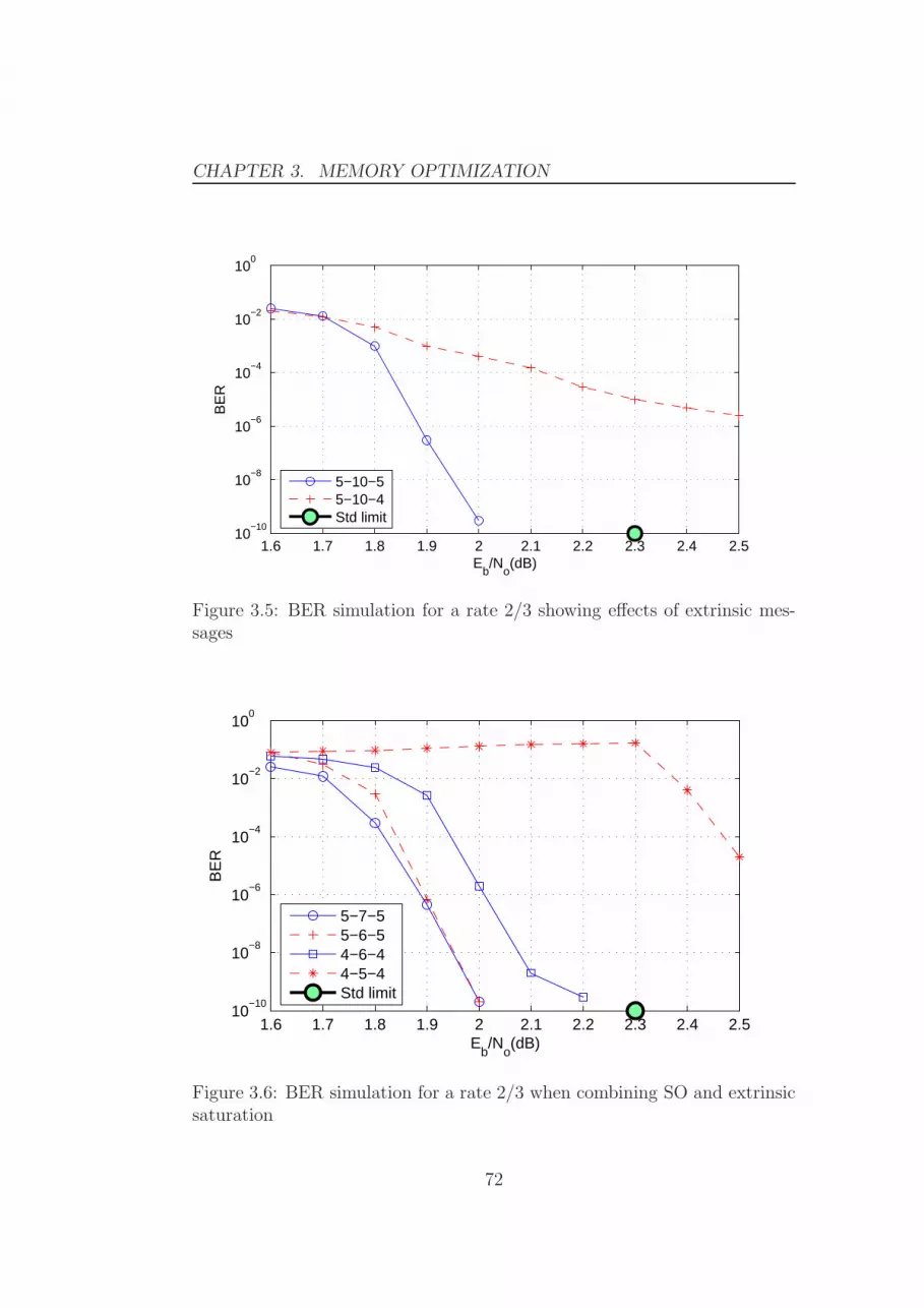
CHAPTER 3. MEMORY OPTIMIZATION
1.6 1.7 1.8 1.9 2 2.1 2.2 2.3 2.4 2.510
−10
10−8
10−6
10−4
10−2
100
Eb/N
o(dB)
BE
R
5−10−55−10−4Std limit
Figure 3.5: BER simulation for a rate 2/3 showing effects of extrinsic mes-sages
1.6 1.7 1.8 1.9 2 2.1 2.2 2.3 2.4 2.510
−10
10−8
10−6
10−4
10−2
100
Eb/N
o(dB)
BE
R
5−7−55−6−54−6−44−5−4Std limit
Figure 3.6: BER simulation for a rate 2/3 when combining SO and extrinsicsaturation
72

3.2. OPTIMIZING THE SIZE OF THE EXTRINSIC MEMORY
Rate M WSign WInd WMc→v Memory
1/4 48600 4 2 14 6804001/3 43200 5 3 16 6912002/5 38880 6 3 17 6609601/2 32400 7 3 18 5832003/5 25920 9 3 21 5443202/3 21600 10 4 22 4752003/4 16200 14 4 26 4212004/5 12960 18 5 31 4017605/6 10800 22 5 35 3780008/9 7200 27 5 40 2880009/10 6480 30 5 43 278640
Table 3.1: Memory size of extrinsic
on 6 bits and Moldc→v on 5 bits gives the same performance as other known
implementation with fewer bits.
3.2 Optimizing the size of the extrinsic mem-
ory
This section focuses on the design of an optimal implementation for elevendifferent code rates. Because the extrinsic memory size requirements stronglydepend on the coding rate, a memory dealing with many coding rate is anissue.
3.2.1 Extrinsic memory size requirements
The memory requirements of each CN is determined by the Moldc→v messages
needed for the CN computation. In the case of the normalized Min-Sumalgorithm, the Mold
c→v values are compressed with min, submin, indmin andsignMc→v. In terms of memory, one address must be allocated for every CNwhich means that the RAM address range (RRAM ) is given by the number ofCNs (M). The RAM word size (WRAM) is given by the size of the compressedMold
c→v values. If we denote by Wh the word size of h, then WMc→v = W|min|+W|submin| + Wind + Wsign. Table 3.1 presents the required memory capacity(M ×WMc→v) for each rate. To calculate WMc→v
, we fix the value of W|min|
and W|submin| to 4 (witout sign). To deal with the eleven code rates of the
73

CHAPTER 3. MEMORY OPTIMIZATION
standard, a simple implementation would define RRAM with the maximumM value, and WRAM with the maximum WMc→v
in Table 3.1. Here, the totalmemory capacity would give: 48600× 43 = 2089800 bits. For rate 1/4, 67%of word bits are wasted but addresses are fully used. On the other hand, forrate 9/10, words bits are fully used but 86 % of the addresses are wasted.Theoretically, a memory size of 691200 bits (maximum memory size in Table3.1) would be enough to cover all the rates. An implementation solution hasto be found for a better utilization of the memory.
3.2.2 Optimization principle
The idea is to add flexibility to both the address range and the word size.For this, we benefit from the fact that the RAM that stores the compressedMold
c→v value is needed only once per layer. As the delay to compute the nextlayer is dc cycles, we can use up to dc cycles to fetch the data in the memory.A word can be split into two if we take two cycles to fetch the data, andsplit in three if we take three cycles. If we consider a single port RAM toimplement the memory, up to ⌊dc/2⌋ cycles can be used to read data, and⌊dc/2⌋ cycles to write new data.
Let us consider the example of a memory bank of size 48600(RRAM) ×22(WRAM). In a first configuration, where one cycle is used, we have amemory size of 48600 × 22 which fits to rates 1/4, 1/3, 1/2, 3/5, and 2/3.In a second configuration, where two cycles are used, and two words of size22 are fetched at consecutive addresses, we have the equivalent of a memoryof size 24300× 44 which fits to rates 3/4, 4/5, 5/6, 8/9 and 9/10. The totalmemory size for the two-cycle option is equal to 48600 × 22 = 106920 bits.This constitutes a memory savings of 50% compared to the straightforwardimplementation.
3.2.3 Results of optimization
The previously described process can be generalized for different word sizes.Table 3.2 gives an example with WRAM = 9. For each rate, the numberof cycles is given by ncycles = ⌈WMc→v/WRAM⌉, and RRAM is deduced from
RRAM = ncycles ×M . The global RAM range (RglobalRAM ) is given by the maxi-
mum RRAM in Table 3.2 and the total memory capacity is RglobalRAM ×WRAM =
97200× 9 = 874800 bits.Fig. 3.7 shows the total memory capacity as a function of the word length
WRAM . There are local minima for word sizes 1, 9, 14, 18 and 21 bits. Asthe number of clock cycle to fetch Mold
c→v is bounded by ⌊dc/2⌋, the possiblesolutions are limited to WRAM greater than 7. A word size of 9 bits gives the
74

3.2. OPTIMIZING THE SIZE OF THE EXTRINSIC MEMORY
Rate M WMc→v ncycles RRAM
1/4 48600 14 2 972001/3 43200 16 2 864002/5 38880 17 2 777601/2 32400 18 2 648003/5 25920 21 3 777602/3 21600 22 3 648003/4 16200 26 3 486004/5 12960 31 4 518405/6 10800 35 4 432208/9 7200 40 5 360009/10 6480 43 5 32400
Table 3.2: Memory capacity of the extrinsic message with WRAM = 9
0 5 10 15 20 250
2
4
6
8
10
12
14x 10
5
Figure 3.7: Memory capacity as a function of WRAM
75
CHAPTER 3. MEMORY OPTIMIZATION
best memory optimization of 874800 bits. This is only 26 % more than thetheoretical minimum.
We used the same memory optimization for an LDPC decoder that im-plement a BP algorithm using Mc→v values that are not compressed (all theMc→v values are stored). We found a theoretical minimum of 1188000 bits,and a total memory size of 1296000 bits with words of size 10.
3.2.4 Case of the sum-product algorithm
When using a sum-product algorithm [49] [28] [23] instead of a Min-sumalgorithm, the check node update equation (1.17) is computed for each Mc→v
value and each Mc→v value are stored. The same process as the previouslydescribed can by used but a simpler and more efficient implementation canbe used. We can consider a dual port ram which is read every cycle to fetcha Mold
c→v value and write simultaneously a Mnewc→v value to be stored. With
the constraint of 11 code rates, 5 bits quantification and dual port ram, thememory requirement is given by the code rate that require the maximumnumber of Mc→v values. The code rate 5/6 requires storing 237600 valuesof 5 bit which give 1.2 MBits memory requirement. Although this size is26% higher than the solution that we proposed for the Min-Sum algorithm,the over cost can worst it, considering the performance increase especially atlow code rate. Implementation of a FIFO memory with single port modulesfor allowing simultaneous read and write operations is presented in [1]. Thissolution requires one memory banks for even addresses and another memorybanks for odd addresses and lead to area saving compared to the use of dualport ram.
3.2.5 Mc→v memory optimization conclusion
The Mc→v memory optimization shows that the implementation of LDPCdecoder for multiple code rate and single port RAM to store the Mc→v is anissue.
A careful implementation of the Min-sum algorithm gives result only 26% more than the theoretical minimum compared to a straight forward im-plementation with 200% over cost.
The sum-product algorithm lead to a 26% over cost compared to the Min-Sum algorithm, but considering performance increase with low code rate, theimplementation of the sum-product can be considered.
76

3.3. FINITE PRECISION ARCHITECTURE OF THE LAYERED
DECODER
SignT
4
Generator
+
dc
+APP
2’s
2’s
6
7
6
RA
M
Sign
2’s
8
FIFO(Dc)
SortingSerial
XOR
Serial
generator
abs4
Check node core
6
2’s
2’s
Ser
ial t
o P
aral
lel
1
−
6SM
→2′ s
SerialMc→v
Sign
Min
Submin
Index
2′ s
→SM |Mc→v|
SM
→2′ s
MV →C
Mc→vMemory
SOin SOnew
Figure 3.8: Finite precision of the NP architecture
3.3 Finite precision architecture of the lay-
ered decoder
Fig. 3.8 presents the finite precision architecture of the NP (Fig. 1.8).Word size, type (signed or absolute) and direction are detailed for everysignal connection. The architecture implements the normalized Min-Sumalgorithm.
In the Check node core, The Mv→c values arrive serially in two’s com-plement representation from the adder modified to implement algorithm 3.They are transformed to sign and magnitude representation so that the signand magnitude of the messages can be computed separately. The serial sort-ing of the incoming magnitude values is implemented, in order to give Min,SubMin and Index values until all the incoming messages are read. In theserial Mc→v block, the Min, SubMin and index values previously sorted areused to serially compute the new outgoing messages. An XOR function iscomputed recursively on the incoming sign bits in the Signt, until all theincoming messages are read. Next, an XOR function is computed in XORblock, between the output of Signt block and the sign of the outgoing mes-sage Mv→c from the FIFO memory of size dc. The sign and magnitude fromXOR block and serial Mc→v block, respectively, are transformed into a two’scomplement representation ready for subsequent computations.
77

CHAPTER 3. MEMORY OPTIMIZATION
6 x 45
45 NPBarrelShifter
RA
M_S
O
BufferChannel
Control
5x45
Figure 3.9: Layered decoder architecture
In the Mc→v memory block, the Min, Submin, index and sign of eachMc→v linked to one check node are stored in a RAM. From theMin, Submin,index and sign values, the serial Mc→v generator computes the two’s comple-ment representation of the Mc→v value.Min and Submin are quantified on4 bits (absolute values) which gives Mc→v values quantified on 5 bits (withthe sign bit). Note that as signt gives the result of the parity check equa-tion of line and the syndrome can easily be computed by using the result ofsignt. The computation of the syndrome allows deciding an early termina-tion of the decoding process leading to a significant reduction of the numberof iterations.
Fig. 3.9 is an overview of the proposed layered decoder architecture (see[46] and [45] for a more detailed description). In this figure, the NP blockis made of 45 NP (Fig. 3.8) working in parallel. The Barrel Shifter shiftsseven words of size 45. The RAMSO block stores the SO values. Thanks to asystematic syndrome calculation, it is possible to use a built-in stopping rulewhile decoding in a variable-iteration decoder. The addition of a buffer onthe decoder input allows the exploitation of the variations in the decodingtime in the different frames. A preemptive buffer control as in [52] is usedto reduce the buffer size. Note that the quantification reduction also leadto area reductions of the node processor and the barrel shifter. The latencyin the Check node core is also reduced due to complexity reduction of theaddition and comparison computation.
78

3.4. RESULTS OF MEMORY OPTIMIZATION
0.5 1 1.5 2 2.5 3 3.510
−10
10−8
10−6
10−4
10−2
100
Eb/N
o(dB)
BE
R
1/41/22/33/44/55/6
Figure 3.10: BER for long frames
3.4 Results of memory optimization
3.4.1 Monte-Carlo Simulations results
Fig. 3.10 shows simulation results for code rates 1/4, 1/2, 2/3, 3/4, 4/5, 5/6and 5-6-5 configuration. The code rates 1/2, 2/3, 3/4, 4/5 and 5/6 showresults that fulfil the standard requirements. The code rate 1/4 shows poorperformances. The code rates 1/4, 1/3 and 2/5 have a check node degreesmaller than 7 (4, 5 and 6 respectively) which lead to an error floor with thenormalized min-sum algorithm. One can note that code rate 1/2 with a checknode degree of 7 start producing an error floor that can be corrected with theBCH outer decoder. This error floor problem can be solved by implementingan A-min* or λ-min algorithm instead of the normalized Min-Sum in theCNP, with no change in the rest of the architecture. One can also implementa Sum-product algorithm as in [33] combined with the proposed saturationprocesses.
3.4.2 Synthesis results on FPGA
The architecture presented in Fig. 3.9 was synthesized on a Virtex-V ProFPGA (XQ5VLX110) from Xilinx, for validation purposes. The system de-codes long frames of code rate 2/3. Table 3.3 gives the hardware resources
79

CHAPTER 3. MEMORY OPTIMIZATION
XQ5VLX85 LUT LUT RAM BRAM
Node Processor 143 2 0sorting 37 0 0
gen mc→v 34 0 0fifo mv→c 12 2 0
mc→v memory 46 0 3Total 1 node 189 2 3Total 45 nodes 8586 90 135
Control 667 3 0
block SO RAM 360 0 22
Channel RAM 48 0 25
Barrel shifter 945 0 0
Total 11005 93 182
Percentage [%] 5 1 50
Table 3.3: Synthesis Results for DVB-S2 LDPC decoder on Virtex-V
required. The clock frequency is 200 MHz, the average number of iterationsis 20 and the throughput is 90 Mbit/s, which allows for the decoding of atleast two simultaneous High-Definition Television (HDTV) streams.
3.4.3 Memory capacity comparison
Table 3.4 shows the number of bits for the main memory units in the lat-est published DVB-S2 decoder IPs [48, 66, 65]. Note that no informationis provided on the ROM memories that store the matrices for every rate.
Paper [48] [66] [65] This
Parallelism 180 360 180 45Air Throughput[Mb/s] 180 135 135 90
Extrinsic quantification [bits] 6 6 6 5SOram quantification [bits] 10 8 8 6Channel quantification [bits] 6 6 6 5
Buffer capacity [Mbits] 0 0 0 0.65Total capacity[Mbits] 2.8 2.83 3.18 2.65
Table 3.4: Memory capacity comparison
80

3.5. A SINGLE PORT RAM ARCHITECTURE
In our architecture, the ROM capacity is 0.1 Mbits. A buffer of size twoframes is used to store the channel LLR values. The buffer combined witha variable iterative decoder 4.4.3 allows increasing the throughput by two.Our architecture provides memory saving of 28% compared to [48], for the5-6-5 configuration (for the 4-6-4 configuration the memory savings is 40%).
3.5 A single port RAM architecture
During the implementation process, the choice between single port and dualport RAM comes into the picture depending on the technologies used. Area,cost, consumption and the complexity parameters have to be also taken intoaccount.
3.5.1 Single port ram, dual port ram, pseudo dual portram and dual port RAM
The difference between Single Port RAM (SPRAM) and Dual Port RAM(DPRAM) is that SPRAM can be accessed at one address at one time, thusyou can read or write only one memory cell during each clock cycle. Dualport RAM has ability to simultaneously read and write different memorycells at different addresses. SPRAM uses a 6 transistors basic RAM cell,while the dual port RAM cell uses 8 transistors cells for memory. So thearea of SPRAM is much smaller than the area of DPRAM cell and is alsomore power efficient. To gain the advantages of both SPRAM (less area) andDPRAM (high speed), Pseudo DPRAM is introduced. Pseudo DPRAM canread and write the data in the same clock, using rising and falling edges forthe operations respectively, and using SPRAM memory cell for the storageof data.
3.5.2 Memories in ASICS and FPGA
In FPGAs, most RAM structures are naturally dual-ported, e.g. the VirtexBlock RAMs. On the other hand, in the ASIC library you can only instantiatesome single port RAM and RAM which can be written in one port and readfrom the other port. This is a powerful FPGA argument if a true dual-portmemory is needed. Because the use of DPRAM is not an issue on FPGA,an implementation on an FPGA of an LDPC decoder for prototyping andtesting purpose is a convenient solution. However, the finale purpose ofthe layered decoder is to be implemented on ASICs for mass production atreduced cost. The studies of a SPRAM solution benefits from reduced area
81

CHAPTER 3. MEMORY OPTIMIZATION
and the fact that the layered decoder will have to be implemented later forASIC solution. We discuss hereafter on existing solutions to change fromDPRAM to SPRAM.
3.5.3 Implementation of dual port RAM with singlePort
For some applications 2 SPRAMs can be used in an alternate buffer configu-ration. For dual read ports and a single write port, two RAMs are used andones always write to both of them together, but read from them separately,with each treated as a separate read port. It is also possible to time-multiplexthe two ports, which will take a double-speed clock and extra logic for themultiplexing.
3.5.4 FIFO memory with single port memory modules
In [1] is presented a FIFO memory with single port memory modules forallowing simultaneous read and writes operations. The method includes thefollowing steps: (a) providing a first SPRAM for an even address of a reador write operation; (b) providing a second SPRAM for an odd address of aread or write operation; (c) alternating even address and odd address; and(d) when both a read request and a write request reach either the first singleport memory module or the second single port memory module at a clockcycle, fulfilling the read request at the current clock cycle and fulfilling thewrite request at the next clock cycle.
3.5.5 Single port memories banks for the SO memories
By looking at an application, it is possible to see whether a full dual-portRAM is really needed, or whether one is dealing with a special case whereit is possible to segregate it into independent parts. The memory can bebuild from multiple smaller RAMs and decode logic added to allow doinga simultaneous read and writing access, as long as they address separateRAMs. If the likely access pattern is known, the chance of collisions canbe reduced by choosing which address bits select a RAM and which onesselect a word in the RAM. In our case, the access schedule to memory is wellknown, and memory conflicts can be predicted and avoided by making surethat distinct memory bank are addresses for read and write operations at anytime. Furthermore the order of the memory access can be modified if needed(layer scheduling and VG scheduling). The number of possible combinationis huge (number of memory bank, addressing scheme in memory banks, layer
82
3.6. LAYER SCHEDULING FOR SINGLE PORT RAM
scheduling and VG scheduling). Finding the best solution will requires thehelp of graph theory but even with the help of graph theory, some parametersand implementation options have to be defined to reduce the space solution.
In [36],to avoid read/write conflicts, the SO memories are partitioned in4 RAMs. A buffer is added to hold the data if writing is not possible due toconflict. The two least significant bits of address determines the assignmentto a partition. This allows a simple control flow, which just has to comparethe reading and writing addresses of the current clock cycle.
With a reduced parallelism compare to [36], a reduced number of RAMconflict can be expected. Our goal is to optimize the best addressing scheduleso that no RAM conflicts arise and no buffer overhead is required.
3.6 Layer scheduling for single port RAM
The order or schedule of the SO arriving in the CNP does not change theresult of the CNP (see Section 1.2.1) and an efficient scheduling of the SO cansolve the read/write conflicts. For ease of understanding we use an example,we then generalize to general case giving problem and solution.
3.6.1 An example with two memory banks
In this example, a structured matrix with dc = 8 is considered and thenumber of VG with even address is equal to the VG with odd addresses (4are even and 4 are odd). Let us focus on one layer with the following VGaddress 1, 2, 4, 5, 8, 10, 13, 15. Usually the schedule follow the VG addressin the increasing order. The schedule is modified such as an even number isfollowed by an odd number i.e. 1, 2, 5, 4, 13, 8, 15. The same process is usedfor the following layers. On this example the layered decoder has a delay of9, which means that 9 cycles are needed between reading a value and writingthe value. When the result of an SO at an even address is written back, anSO at an odd address is read. If all the even address are stored in memorybank (MB1) and all the odd address are stored in memory bank two (MB2)then it is possible to use single port RAM without risk of conflict and onlytwo memory banks. In case of delay that is even, then a buffer of depth oneis required in order that the writing operation fall in the previous describedsolution.
As the Less Significant Bit (LSB) address give the parity (odd or even),the implementation is straight forward by storing the SO in MB1 or MB2depending on the SO address LSB. The benefit is the use of SPRAM insteadof DPRAM. The drawback of this solution is that a structured matrix with
83

CHAPTER 3. MEMORY OPTIMIZATION
a specific constraint is required. This could be an interesting constraint forthe design of architecture aware codes.
3.6.2 Generalization for DVB-X2 matrices
There is not always the same number of odd and even address in a layer.A solution is to switch one or some address from even to odd, or odd toeven in order to fall in the configuration of the example. This switching ofaddress would lead to an implementation over cost and even by trying all thepossibilities, there is sometime no solution.
To give much more possibility, 4 memory banks are used as in [36]. Theimplementation is fixed and simple with the two LSB addressing the 4 mem-ory banks. To solve read/write conflicts, the fact that VGs in a layer can bepermuted is used. If there is a read/write conflict between two VG, one ofthen is permuted and provided that the permutation does not lead to anotherconflict then the conflict is solved. As the number of possible permutation ishuge, a brute force approach is not possible and the help of graph theory isneeded.
3.6.3 Genetic algorithm to solve scheduling problem
The advantage of using the Genetic algorithm (GA) is that we already usedthis powerful tool to solve memory update conflicts by the scheduling of thelayers 2.5. Some modifications are required but the tool is ready. This time,the VG in a layer are permuted and the schedule of the layer is fixed. Thiswork is not finalized yet.
3.7 Conclusion
In this chapter, a memory optimization for a layered LDPC decoder hasbeen presented. A first approach to memory savings was to analyze the sat-uration problem in the layered decoder. A second approach relied on theword split of the extrinsic memory. We developed a finite precision layereddecoder architecture that implements the proposed saturation process. Thisarchitecture outperforms the state-of-the-art in terms of memory needs whilesatisfying the standard requirements in terms of performances. A method-ology is also given in order to implement single port RAM instead of dualport RAM in the layer decoder leading to significant space saving. Even ifthe DVB-S2 standard is considered in this chapter, the proposed techniques
84

3.7. CONCLUSION
can be extended to the DVB-T2 and -C2 standards and, more generally, toany layered LDPC decoder.
85

CHAPTER 3. MEMORY OPTIMIZATION
86

Logic will get you from A to
B. Imagination will take you
everywhere.
Albert Einstein (1879-1955)
4Multi Stream LDPC decoder
Summary:In this chapter, the goal is to find a way to reduce the cost of decoding x
streams by using one decoder compared to the solution of using x decoders.The state of the art gives solutions based on increasing the parallelism, shar-ing resources or inserting a buffer to a variable iteration decoder. Thesethree options are considered and developed to satisfy our case study. Thenan architecture supporting multiple streams is presented
4.1 Introduction
Multi stream decoder can be interpreted in two ways. First, it can be inter-preted as a decoder able to decode multiple kinds of standards. To be morespecific, for television broadcasting, many stream standards exist:
• Standard-Definition Television (SDTV) streams,
• Extended-Definition Television (EDTV) streams,
• High-Definition Television (HDTV) streams,
• Three Dimensions Television (3D TV) streams.
From the LDPC decoder point of view, the difference between these standardsis only in terms of required throughput. The bandwidth is highly dependenton the standards listed here:
87

CHAPTER 4. MULTI STREAM LDPC DECODER
• the bandwidth consumption of SDTV (720 x 480 pixels) is about 5Mbps,
• the bandwidth of HD TV (1920 x 1080 pixels) stream is about 13 Mbps,
• 3D Blu-ray uses about 50% more throughput than HDTV dependingon the compression,
• in case of 3D TV based one HD image per eye; the bandwidth is thedouble of one HD TV stream.
Between single SDTV stream and a 3D TV stream, there is a factor 5 inthroughput requirement. In this interpretation, a multi stream decoder hasto fulfill the highest required throughput.
The term Multi stream decoder can also be interpreted as a decoder de-coding simultaneously x streams. Double or twin tuners make the differenceon the market when customers want to record a movie while watching an-other. A video surveillance application can require up to 32 streams at 30frames per second simultaneously. The required throughput in these casesare simply multiplied by x. In both interpretations, multi stream LDPCdecoder is a matter of throughput. Combining the two interpretations inone decoder, i.e. a dual stream 3D TV decoder, the throughput will varyfrom one STD stream to two 3D TV streams, which makes a factor 10 inthroughput variation. The decoder will be designed for the worst case whichmeans the highest throughput but energy saving should be managed whenthe decoder is under exploited. A straight forward implementation of a multistream decoder would use x decoders in parallel.
In this chapter, we present the case of one decoder decoding x streamsand optimize area saving compared to the straight forward solution. The onedecoder solution is studied through three axis. The first one gives flexibilityto the throughput of a given layered decoder by reordering the matrix infunction parallelism. The second axe presents an architecture allowing shar-ing resources for a dual stream LDPC decoder. The third option presents avariable iterative decoder associated with a buffer allowing increasing nearlyby two of the throughput. Finally, an architecture is presented.
4.2 The parallelism option
The matrices given in the DVB-S2, -T2 and -C2 standards are structuredfor a parallelism of 360. The split process of the matrices used to reduce thenumber of conflicts [45] [46] described in Chapter 2 can also be used to gain
88

4.2. THE PARALLELISM OPTION
Ps 36 40 45 60 72 90 120 180 360
100 MHz 42 47 53 70 84 106 141 212 423200 MHz 84 94 106 141 169 212 282 423 845400 MHz 169 188 212 282 338 423 564 846 1691
Table 4.1: Throughput (Mbit/s) as a function of the parallelism Ps and theClock frequency with itcst = 17 and ǫ = 6
flexibility in the parallelism and thus in the throughput. The parallelism canbe reduced by using the splitting process to P = Ps provided that 360 =Ps × S where Ps and S are natural numbers. Note that in [13] a method isproposed in which the parallelism factor does not have to be a divider of theoriginal expansion size (P =360). This solution gives freedom of choosing aparallelism factor that fits exactly the required throughput. The throughputof a pipelined layered LDPC decoder is given by the following equation:
D2 =K.FClk
dc.MPs.itcst + dc + ǫ
bit.s−1 (4.1)
where itcst is the average number of iterations to decode a codeword, M isthe number of CN, Ps is the number of CNPs working in parallel, dc is theaverage number of VNs linked to a CN, Fclk is the clock frequency, K is thenumber of information bits in a codeword and ǫ is the CN latency.
Table 4.1 gives an idea of the throughput in function of the parallelismand the clock frequency when using standard frame and coding rate set at2/3, ǫ = 6. A buffer is added to the decoder as presented in Section 4.4which reduces itcst = itmax = 30 to itcst = 17 = itavr .
4.2.1 Area saving compared with x decoders and con-clusion
To give an idea of area saving, we compare the parallelism solution with a xdecoders solution. In our case of study, an LDPC decoder for one HD streamgives in term of area 75 % of memory, 20 % of CNP and 5 % of control. Todecode a dual stream for a given throughput, two decoders decode two framessimultaneously with a parallelism of p while one decoder decodes one frame ata time with parallelism of 2p. For the one decoder solution, the parallelism isdoubled but the control and the memory required is unchanged. Comparedto a two decoders solution, the area saving is 40 %. Generalizing with xstreams, the parallelism option save x− 1 memories. The area saving is 53%
89
CHAPTER 4. MULTI STREAM LDPC DECODER
for x = 3 and 60% for x = 4.
The parallelism option allows to fit with the various throughput require-ments and provides significant memory and area savings compared to a xdecoder solution.
4.3 Share resources in a dual stream decoder
A Block-interlaced LDPC decoder is proposed in [12] with an architecturebased on the flooding schedule. The interlacing technique processes twoframes simultaneously. In this section we apply the interlacing technique toa layered decoder and we discuss its advantages and drawbacks.
4.3.1 Sharing principle
As shown in Section 1.2.2 the check node update is split into two steps ofdc cycles. First step, the data are read, and second step, the updated dataare written back. These two steps can easily be pipelined by overlapping theupdate of two layers. When one layer is updated in step one, another layeris updated in step two. The pipelined scheme in Figure 2.17 doubles thedecoder throughput compared with the throughput in Figure 2.16.
Instead of overlapping two layers of the same frame, the decoding oftwo consecutive frames is interlaced. While a layer is reading frame onein step one, another layer is writing frame two in step two. For layereddecoders, block interlacing keeps the CNP unchanged but requires doublingthe LLR and Mc → v memories so that the CNPs can switch between thetwo memories as they switch between the two different frames.
4.3.2 Advantages, drawbacks and conclusion
This solution has four advantages compared to a pipeline solution. Firstadvantage is that, the conflicts due to pipeline as describe in Section 2.5 areavoided because there is no SO in common between two consecutive layers.Second, there is no more need of a simultaneous read and write access to theLLR memories. Instead of using dual-port RAM for the LLR memory, singleport RAM can be used without reading and writing conflict risk , leadingto significant area saving. Third advantage is that the area is saving p CNPcompared to a two (not pipelined) decoder solution. Fourth advantage: Table2.4 shows that there is no solution for conflicts due to pipeline with highparallelism and block interleaving avoids this conflict.
90

4.4. USE OF A BUFFER
There are two drawbacks of this solution. First drawback is that at con-stant throughput, compared with 2 pipelined decoders, an interlaced decoderdoes not lead to area saving. The interlaced solution needs as much memoryas the two decoder option and to have the same throughput as one pipelineddecoder, the parallelism of the interlaced decoder need to be doubled. Sec-ond drawback is that the streams need to be at the same rate. In case oftwo streams at different rates, which means the dc are not equal, idle timehas to be inserted to the smallest dc so that the pipelining process can work.The rate problem can be solved by adding a buffer and some kind of controlso that only frames of the same stream are decoded simultaneously but thebuffer size need to be nearly doubled compare to a non interlaced solution.
These drawbacks make this solution not relevant for low parallelism, nev-ertheless in case of high parallelism, this solution becomes more relevant. Inparticular, with a parallelism of 180 or 360, there is no simple solution tosolve conflicts due to pipeline (See Table 2.4) and the interlaced architecturesolves the problem.
4.4 Use of a buffer
Low-density parity-check (LDPC) decoders can be designed in a way theystop after a variable number of iterations, dependent on the difficulty ofdecoding noisy received words. The number of iterations the decoder spendson a given frame determines both the probability of successful decoding, andthe time expended. Thanks to the systematic syndrome calculation, it ispossible to use a built-in stopping rule while decoding in a variable-iterationdecoder. The addition of a small buffer on the decoder input allows theexploitation of the variations in the decoding time of the different frames.Whereas the speed of an LDPC decoder without a buffer is determined by themaximum number of iteration itmax frames, the speed of a variable-iterationdecoder with sufficient buffering is determined by average number of iterationitavr . The addition of an input buffer to an iterative decoder is presentedin [52] and is summarized in Figure 4.1. The buffer, the variable iterationdecoder and the preemptive buffer control are described in the followingsubsections.
4.4.1 FIFO buffer principle
FIFO (First In First Out) memories have acquired larger interest in VLSIdesign in telecom applications. Such macro cells provide an efficient wayto interface two asynchronous system, buffering data between subsystems
91

CHAPTER 4. MULTI STREAM LDPC DECODER
Stream
buffercontrol
N
Variableiterative decoder
of size BBuffer
New frame
Full
Empty
Preemptive
Figure 4.1: Variable iteration decoder with a buffer
operating at different data rates, thus increasing the flexibility in data trans-mission. In fact, data in FIFO memories are read in the same order in whichthey have been written, without the need of providing the address of thedata.
Different approaches have been considered in literature to design FIFOmemory cells. The architecture is based on SPRAM cell as described inSection 3.5.4. A generic architecture is defined whose size can be modifiedwith slight modifications to the basic structure. In order to obtain such aresult, two blocks are defined: the memory block which instantiate SPRAMand the control logic block. The control logic is in charge of detecting twoparticular states of the FIFO which are full and empty that will have effectson the decoding process. The empty message says to the decoder that afterthe current decoding, the decoder can switch to a stand-by mode to saveenergy consumption. The use of the full signal is discussed in the followingsubsection.
4.4.2 Preemptive buffer control
Before the buffer gets full, the full signal is sent to the decoder for an earlytermination of the decoding process and the first in data of the FIFO is sentto the decoder to let one space in the buffer to avoid a dramatic overflow. Anoverflow would lead to the lost of one frame while the effect of stopping thedecoding process is limited. The effect of stopping the decoding is limitedfor three reasons: first reason is if the word under decoding is hard to decode(pseudo codeword or cycle trap), spending more iteration would not give so-lution. Second reason is that the degree of parity bits is only two and the
92

4.4. USE OF A BUFFER
convergence of bit with low degree is slower than nodes with higher degree.For this reason, the errors are most probably in the parity bits and not in theinformation bits; this means that even if the stopping criterion is not valid,the information bits can be valid. Third reason is that in case that just alittle more iteration would have been necessary to solve remaining bits, thenthe BCH can solve the last erroneous bits if the number of erroneous bit islower than the BCH capability. Compared to a standard buffer, the preemp-tive buffer control significantly reduces the size of the buffer and reduce theaverage number of iteration to decode even with a buffer of size one.
4.4.3 Variable iterative decoder
A variable iterative decoder is able to detect that a codeword has been found.This solution allows starting the decoding of a new frame. The detection ofa valid codeword, in theory is done by computing the syndrome and checkingequation (1.1). In practice, the syndrome computation can be done duringthe sign calculation of the Mc→v message (See Section 1.2.2). The first stepof the sign calculation gives:
signt(v′) =∏
v′∈vc
sign(Mv′→c) (4.2)
which is in fact the hard decision of the parity check of CN c. If all the harddecisions of all the check nodes are valid then a codeword has been foundand the iterative process can be stopped. This stopping criterion is easy toimplement on a layered decoder and requires a very low cost control. Becausethe decoding time of the variable iteration decoder is not constant, a buffer isrequired at the input of the decoder to smooth the decoding time variation.
4.4.4 FIFO Buffer size
A buffer of size one would be in charge of storing the LLRin of every bitof the codeword. The size of a codeword of a DVB-X2 decoder is N=64800and the quantification of the LLRin in our architecture is 5. The storagerequirement of a buffer of size x is 64800× 5× x which makes the buffer sizethe most critical point of the solution in terms of area. Therefore, the buffersize must be chosen carefully.
The calculation of the optimal buffer size and the average time to decodecan be estimated using queuing theories and the probability distribution ofthe number of iterations (see Figure 1.6). Queuing theory is the mathemat-ical study of waiting lines, or queues. The theory permits the derivationand calculation of several performance measurements including the average
93

CHAPTER 4. MULTI STREAM LDPC DECODER
waiting time in the queue, the expected number waiting and the probabilityof encountering the system in certain states such as empty and full.
The calculation of the buffering requirement by using queuing theorieshas been already presented successfully in [37]. In this subsection, a moreempirical approach is described to determine the optimal buffer size. In fact,a simple patch has been added to the already existing simulation environmentof the LDPC decoder and a Monte-Carlo simulation has been lunched for dif-ferent buffer sizes. The goal of the simulation is to find the best compromisebetween buffer size, number of iteration and performance loss. We presentfirst a simple patch simulating a single stream, and then we generalize witha patch simulating multiple streams.
The algorithm patch can be described by the three following points: a newframe is added to the buffer every itcst iterations; the buffer is decrementedevery time a codeword has been found; and if the buffer is full, then thedecoder stops the decoding of the current frame and takes a new frame inthe buffer to relax the buffer.
Algorithm 4 buffer simulationit← it+ 1if it = itcst thenBuffer← Buffer + 1it← 0
end ifif (word decoded = true)AND(Buffer > 0) thenBuffer← Buffer − 1
end ifif buffer > buffer size − 1 thendecode next()word decoded=trueit← 0
end if
The patch is sum-up in Algorithm 4 where itcst is the average number ofiteration a decoder spend to decode a codeword. Figure 1.6 shows the PDFof the number of iteration before a codeword is found. On the figure itmax
and itavr are also presented . The itmax value is the maximum number ofiterations that a decoder spend to decode a codeword and the itavr value isthe average number of iterations before a codeword is found. On a decoderwith a constant number of iteration to decode, itcst is equal to itmax. Theadvantage of a buffer associated with a variable iterative decoder is that itcstget closer to itavr but even with a huge buffer size, itcst can not be lower than
94

4.4. USE OF A BUFFER
the average number of iteration itavr to decode a codeword. Thus, itcst willbe between itavr and itmax. As shown in equation (4.1), the throughput isdirectly proportional to itcst and has to be as low as possible. The goal of thesimulations is to optimize itcst and buffer size to a minimum with the sameperformance as a decoder with a constant number of iteration to decode fixedat itcst = itmax = 30.
Simulations on a decoder with a parallelism of 40 show us that a bufferof size two gives already the required performances. The performances canbe slightly improved by using a buffer of size 3 and a buffer of size greaterthan 3 does not give significant improvement. With a buffer size two, itcst =17 which is close to itavr = 16 and nearly the half of itmax thus nearlydouble the throughput compared to a constant iterative decoder. Note thatonce itcst is found, one should check if Equation (4.1) gives a throughputhigher than the required throughput, and if not, increases the parallelism inproportion. Note also that the simulation emulates on an ideal case makingsome assumptions which are simplifying the architecture constraints. Amongthe simplifications, we consider that the FIFO buffer is read and writtenwithout latency, the decoder can stop a decoding process without delay,and decoder load a new word without latency. These assumptions can beacceptable if the latencies are negligible compared to the time unit of thesimulation which is expressed in terms of iterations.
A SDRAM with a transfer rate of 64bit per cycle would require at least6075 cycles to transfer the 64800 × 6 bits of one frame which is roughlyequivalent to one iteration time for a rate 2/3 with a parallelism of 40.
In case of multi stream, if the streams are serialized, then Algorithm 4can be used without modifications. If the streams arrive in parallel, then thepatch is modified as follow: n frames are added to the buffer every n× itcstiterations. The Algorithm 4 is upgraded to Algorithm 5 where RAMwrite
and RAMread represent the time to write (read) a new frame in number ofiteration.
For dual stream, with a decoder with doubled parallelism, simulationsusing Algorithm 5 show us that a buffer of size 5 fulfill the required perfor-mances.
4.4.5 Advantages and drawbacks
The only drawback of this solution is the buffer size. The main advantageof this solution is the improved throughput by nearly two. It is also possibleto get advantage of additional iterations to decode a codeword if the bufferis empty by increasing itmax. In the same way of thinking, itmax can evolvein function of the buffer state. If the buffer is about to get full then decrease
95

CHAPTER 4. MULTI STREAM LDPC DECODER
Algorithm 5 buffer simulation 2it← it+ 1if it = n× itcst thenit← 0
end ifif it = n× itcst −RAMwrite thenBuffer← Buffer + n
end ifif it = RAMreadAND(Buffer > 0) thenBuffer← Buffer − 1
end ifif buffer > buffer size − 1 thendecode next()it← 0
end if
itmax and if the buffer is about to be empty then increase itmax.
4.4.6 Implementation issue
The parallelism option and the addition of a buffer give the throughput andflexibility required by the decoding of multi streams. The parallelism optionhas been integrated in the design of the VHDL code as a parameter. Tochange parallelism, the parallelism parameter is changed and the VHDL issynthesized again to implement the modification.
The circular buffer can be implemented using a FIFO associated with anappropriate control. The control is in charge of sending the full signal andthe empty signal. In case of multi stream, for example dual stream decoder,the FIFO can be modified to have two inputs and one output. Figure 4.2shows an architecture example where two streams are filling the top of thebuffer. Another buffer is added to the output of the decoder to synchronizewith the BCH. The output buffer stores the hard decision of the decoder andthe buffer control is in charge of reordering the stream one and two.
The buffer can be implemented in Synchronous Dynamic RAMs (SDRAMs)to save cost. SDRAM devices are low-cost, high-density storage resourcesthat are widely available. To reduce the read and write operation latency,the SDRAM can be read and write by using a burst-mode. For a dual streamdecoder, two memory banks are written simultaneously while one memorybank is read. Two memory banks are added as FIFO storage (See Section4.4.4). This makes a total of 5 memory banks.
96

4.5. CONCLUSION
control
Stream 2
Stream 1
Variableiterative decoder
New frame
Full
Empty
Stream 1
Stream 2
buffer
Figure 4.2: Variable iteration decoder with a buffer
The loading of a new word in the decoder can be time consuming andreduce the throughput. One solution is to use two SO memories in “pingpong”. While one memory is used for the decoding process, the other oneis loading a new word. When a codeword is found, the two memories areswitched.
4.5 Conclusion
The fact of sharing resources to decode two streams simultaneously givesmore drawbacks than advantages, especially at low parallelism. The paral-lelism option combined with the addition of a buffer gives the throughputand flexibility required by the decoding of multi streams. The parallelism ofthe decoder is chosen in function of the required throughput. To deal withthe variable throughput requirement, a buffer added to a variable iterativedecoder gives furthermore the advantage of reducing the average number ofiterations the decoder spend to decode a codeword.
97

CHAPTER 4. MULTI STREAM LDPC DECODER
98
An investment in knowledge
always pays the best interest.
Benjamin Franklin(1706 - 1790)
5Conclusion
In this thesis, we provide solutions for implementing an LDPC decoder forthe second generation Satellite Digital Video Broadcast (DVB-S2) standard,the DVB-T2 (terrestrial) standard and the DVB-C2 (Cable) standard.
In Chapter 1 we introduced the advanced techniques of channel decod-ing. After a brief overview of digital communication and channel decoder,notions and notations of Low Density Parity Check (LDPC) codes have beenpresented and more specifically the layered decoder and the Believe Propa-gation (BP) sub-algorithms are detailed. Then the LDPC included in theDVB-S2, -T2 and -C2 standards is presented with the state-of-the-art of ex-isting implementations. Finally, we present a testing environment designedto evalutate the performance of error correcting codes. From the state-of-the-art of exiting implementations, the layered decoder is identified as themost efficient architecture. This architecture uses the Normalized Min-Sumalgorithm for the check node update because of its good performance andlow area cost of implementation. In the aim of most efficient implementation,the check node processors are pipelined to double the throughput.
The implementation of this defined architecture led in practice to memoryupdate conflicts. Two types of memory update conflicts have been identifiedin Chapter 2: the conflicts inherent to the presence of overlapped sub-matrices and the conflicts due to the pipelined architecture. To improvedthe exiting solutions, we decided to find a pach free solution to keep theefficiency of the layered decoder.
99

CHAPTER 5. CONCLUSION
We proposed two innovative solutions to solve the conflicts inherent tothe overlapped-sub-matrices. The first solution that we presented in [45] isbased on a “divide and conquer” strategy. The number of conflict is firstreduced by a reordering mechanism of the matrix called split algorithm thatcreates a new equivalent structured matrix with reduced parallelism. Withthis first step, lower is the parallelism and lower is the number conflicts.
The remaining conflicts are solved with a “split-extended” matrix. Thesplit extend proced operates on deficient layer by cutting the layer in twoseparate layers. Each obtened layer contain one of the overlapped submatri-ces. To keep the check equation valid, the two layers are extended with acommun group of dummy bits. This first solution is efficient especially forlayered decoder that can deal with not constant check node degree and lowparallelism.
The other solution is in a patent process and it is based on a repeat ofthe deficient layers and an “on time” write disable of the memories. Thissecond solution is especially efficient for architecture using not compressedextrinsic memory and is efficient even at high parallelism.
The two proposed solution are not 100% patch free, but the added com-plexity is low and require just a slight increase of control. This added controlis not in the critical path and does not degrade the throughput.
In Section 2.5 and in [46], we solve the conflicts due to pipelining. Thesplit process is used again as a first step. This first step reduced conflictconstraints allowing finding solutions by a scheduling of the layers. Thelayer scheduling required the need of graph theory to be solved in a reaonablecomputing time. We showed that the research of an efficient scheduling isequivalent to the well known ”Traveling Salesman Problem” (TSP). Then agenetic algorithm heuritic has been used to solve the TSP.
All the proposed method are compatible between each other. It meansthat the methods can be combined in a single implementation to solve bothconflicts due the overlapped matrices and conflicts due to pipelining.
After the memory conflict problems solved, we focused on finding differentways of optimizing the layered decoder implementation in Chapter 3. As80% of the decoder is memory, we explored how to reduce the memory size.The memory is directly proportional to the word length and we reduce it bya specific saturation. We identified the saturation effects determinig whichvalue are less sensitive to aturation and we conteract unwanted effect ofsaturation. cost in memory and .interaction between the SO values and theextrinsic messages. Then we presented a finite precision layered decoderarchitecture that implements the proposed saturation processes. With allthe code rates, extrinsic memory address range and word size are subject to
100

5.1. PRODUCED WORK
significant variation. We discussed the best way to implement this variationwith the minimum memory over cost. The saturation process and extrinsicmemory optimization have been presented in [44] and implemented on anFPGA giving performances in the standard requirement and significant areareduction compared to the state-of-the-art. After that, still in the memoryoptimization field, we discussed efficient solutions to implement the LDPCdecoder using only single port RAM instead of dual port RAM. Once theconflicts have been solved and the layered decoder has been optimized, wefinally focused on the multi-stream problem.
In chapter 4, we explored the problematic of finding the best way toimplement a decoder that decodes multiple streams simultaneously. In ourproposed solution, the parallelism of the decoder allows to reach the requiredthroughput while the addition of a buffer to one variable iteration decodergives an answer to the flexible throughput requirement.
5.1 Produced work
Besides the publication and searching process [45, 46, 44], we also producedgeneric tools useful for the testing and designing of an LDPC decoder. Firstof all, we produced a general ANSI-C model of an LDPC decoder with theassociated testing environment to test the possible algorithms and schedulingoptions. The following step was to design another ANI-C model close to thelayered architecture for co-simulation C-VHDL. Then we have implementedon FPGA two versions of LDPC decoders. The first decoder implemented is ageneric layered decoder. This decoder is able to decode any true layered codessuch as codes defined for the WiMAX and WiFi standards. The implementeddecoder is also able to decode DVB-S2, -T2 and -C2 codes but only for someparallelisms where no overlapped sub-matrices appear. This version allowsalso scheduling layers and thus avoiding memory update conflicts due topipeline as described in Section 2.5. An upgraded version of the layereddecoder allowing repeating layers and controlling the write enable of theSO and extrinsic memory have been designed. This second version is able todeal with the conflict due to overlapped sub-matrices and it is relevant for theDVB-X2 standards and also for the Chinese Multimedia Mobile Broadcasting(CMMB) standard.
To test the efficiency of the LDPC decoder even at low bit-error rate (be-low 10−10), a testing environment has been designed. The testing environ-ment has been designed in C and VHDL which allows C-VHDL co-simulation.The testing environment is an efficient tool to test, to design and to debugan LDPC decoder or in fact any channel decoder.
101

CHAPTER 5. CONCLUSION
5.2 Perspectives
Future work will be dedicated to the hardware implementation optimization(area, frequency and performance) of the proposed decoder architecture andto the evaluation of its performance at low bit error rate. The implementationof a Bose and Ray-Chaudhuri (BCH) decoder is also considered to completethe transmission chain of the testing environment. Implementing and testinga multi stream decoder with the associated buffer and control should be doneto confirm our estimation of the optimal buffer size (see Section 4.4.4).
The performance of low code rates (1/4, 1/3, and 2/5) should be slightlyimproved to fulfill the standard requirement. One solution consists in upgrad-ing the Normalized Min-Sum Algorithm to a λ−min or A−min∗ algorithm.To achieve this, a patch with Look up table can be added to the check nodeprocessors without significant modification in the architecture. An upgradedversion of the existing layered decoder is also considered. This upgradedversion would be able to decode all rates and would implement the struc-ture of the extrinsic message memory proposed in Section 3.2. This versionwould integrate the upgraded Min-sum algorithm that fulfills the DVB-X2requirement for low rate codes.
Standards give lots of challenges to today’s researchers and to all workingin this field to find improvement options. An improving solution which wouldprovide better reception to the customers and would enable to offer betterservices by keeping the costs in a reasonable range or even decrease it. Thecurrent economic crisis, the demanding market needs urge the companies andthe researches to find answers and respond to these great challenges. Thisthesis has a potential answer to a small part of these challenges, but certainlyan important one.
102

Simplicity is the ultimate so-
phistication.
Leonardo da Vinci(1452-1519)
ADVB-S2 matrices construction
The DVB-X2 standard provide a guidline to construct matrices. The result-ing matrices are structured but they are not made of shifted identity matricesas the matrices defined by the WiFi or WiMAX standards [60] and they arenot ready for layered decoding. Some permutations are required to make theidentity matrices appear. In this appendix, a simple example is provided tovisualise the initial structure of the matrices, the required permutations andthe final structure.
A.1 Standard matrices construction
The matrices defined by the standard fall in the IRA codes types. Thematrices are caracterized by two parts: the information part is linking theInformation VNs (IVN) to the CNs and the parity part linking the ParityVNs(PVN) to the CNs. The standard provides a matrix construction proto-col for the information part relaying on the use of a table and an equation.For ease of understanding, in this example a parallelism of 8 instead of aparallelism of 360 and codeword length of 40 instead of 16200 are given. Inthis example, coding rate is 2/5 and q = 3.
Table A.1 has only three values in it but will be used as a table from thestandard (Table 1.3). The values in the first line give the connection betweenthe first eight VNs (IV N0 to IV N7) and the CNs. A value x in the table is
103

APPENDIX A. DVB-S2 MATRICES CONSTRUCTION
2 7
1
Table A.1: example table
IVN PVN
CN
0 7 8 0 7 15 230
7
15
23
Figure A.1: matrix resulting from Table A.1
computed in Equation (1.19) with the new parameters p=8 and q=3.
CNj = CNj ⊕ IV Nm, j = (x+ q(m mod 8)) mod M. (A.1)
The first value in the first line of the table by applying Equation (A.1)will give the connections between V N0(m=0) and CN2, V N1(m=1) and CN5,and so on. The value in the second line gives the connection between thesecond group of eight VNs (V N8 to V N15) and the CNS.
The fixed zigzag connectivity of the PVN and CN is defined by the en-coding scheme given by equation A.2.
CNj = CNj ⊕ CNj−1, j = 1, 2, . . . , N − 1. (A.2)
Figure A.1 shows the resulting parity check matrix. For ease of lisibility,the 0 in the parity check matrix are not presented and the 1 are representedby a colored square. The square colors correspond with the x value given inTable A.1.
104

A.2. MATRIX PERMUTATIONS FOR LAYERED STRUCTURE
IVN PVN
CN
0 7 15 7 15 23
7
15
23
Figure A.2: First permutation
A.2 Matrix permutations for layered struc-
ture
The permutation process is splitted in two steps. First a permutation of theCNs with the permutation equation A.3
σ(j + i× 8) = i+ (j ×Q) mod N, i = 1, 2, 3 j = 1, 2, . . . , 8. (A.3)
Figure A.2 shows the result of this first permutation. It can be seenthat the information part of the matrix is now made of identity matricesbut the parity part needs a permutation of the PVN. The second step is apermutation of the PVN by following the permutation of Equation (A.3).
Figure A.3 shows the resulting matrix made of IM of size 8. One canobserve the particularity of the IM in the upper right corner where the con-nection between the first CN (CN0) and the last PVN (PV N23) does notexist. This particularity can be easisly implemented but can not be ignored.
From the layered decoder point of view, this permutation allows an effi-cient decoding of the DVB-X2 matrices. One will note that a permutationof the PVN is required before the decoding process and a patch is needed forthe upper right identity matrix.
105

APPENDIX A. DVB-S2 MATRICES CONSTRUCTION
IVN PVN
CN
0 7 15 7 15 230
7
15
23
Figure A.3: Second permutation
106
It does not matter how slowly
you go so long as you do not
stop.
Confucius (551BC-479BC)
BHardware Discrete Channel Emulator
B.1 Introduction
The emulation environment named Hardware Discrete Channel Emulator(HDCE) has been developed as a coherent framework to emulate on a hard-ware device (FPGA as the implementation platform ) and simulate on acomputer the effect of an Additive White Gaussian Noise (AWGN) in a baseband channel. The HDCE is able to generate more than 180 M samplesper second for a very low hardware cost, which has been achieved in an effi-cient architecture. Using the HDCE, the performance evaluation of a codingscheme for a BER of 10−9 requires only one minute of emulation time.
In the state-of-the-art, a Random Value (RV) with an uniform distri-bution is generated, and this uniform distribution is modified to obtain agaussian distribution [26, 6, 39]. This accurate white gaussian noise is addedto a signal and then quantified. With the HDCE, a quantified output withthe required distribution is directly produced.
The uniform distribution is generated using a Linear Feedback Shift Reg-ister (LFSR) presented in the first section. Then the alias method is devel-oped and the architecture is presented.
107

APPENDIX B. HARDWARE DISCRETE CHANNEL EMULATOR
Figure B.1: LFSR
B.2 Linear Feedback Shift Register
A Linear Feedback Shift Register (LFSR) is a shift register whose input isa linear function of its previous state. LFSR can produce a sequence of bitswhich appears random. In Fig. B.1, LFSR are concatened in a FIFO givingan efficient implementation of a RV generator. Two control signals read seedand load seed are added to allow the possibility to load the LFSR and toread the LFRS in order to be able to replay a sequence.
B.3 The alias method algorithm
The alias method was initially proposed by A. J. Walker in [67]. The aliasmethod algorithm can be described in two steps. In the first step, two in-dependent uniform distributions Ps0 and Prv are generated. In the secondstep, a test is performed on Prv. If Prv < Threshold(Ps0), then the systemoutput is Ps0. Otherwise, the system produces the alternative value givenby Ps1 = alias(Ps0). The alias values and the threshold values are stored inthe alias table. With a given alias table, a distribution can be predicted. Itis also possible to give an alias table in function of the required distribution.The computation of the alias table can be done by software and then thealias table can be updated.
108

B.4. THE HDCE ARCHITECTURE
Figure B.2: HDCE architecture
B.4 The HDCE architecture
The implementation of the alias method is straight forward by followingthe alias method algorithm. A RV generator is instanciated by the use ofLFSR and produces the Ps0 and Prv signals. A RAM stores the alias tableand produces an Alias signal and a Treshold signal as a function of Ps0. Acomparator compares the two values Treshold and Prv and produces a signalwhich drives a multiplexeur that selects the Pso signal or the Alias signal.Figure B.2 shows an improved HDCE architecture. In this architecture, oneuniform distribution is split to generate the two uniform distributions Ps0and Prv. The comparator is pipelined to decrease the delay and an index isadded to address different distributions.
B.5 Resulting distribution
Figure B.3 shows the Probability Density Fonction of the HDCE outputwith the following parameters: channel quantization on 5 bits, thresholdquantification on 10 bits and two distributions. The two ditributions are
109

APPENDIX B. HARDWARE DISCRETE CHANNEL EMULATOR
Figure B.3: Resulting distribution of a BPSK modulation emulated by HDCE
emulating a BPSK modulation (-1 and +1) which is perturbed by an AWGNof variance σ = 0.866 (corresponding to a Eb/No = 2 dB).
110

Rien ne vaut la recherche
lorsque l’on veut trouver
quelque chose.
J.R.R.Tolkien (1892-1973)
CResume etendu
ResumeThis is a french extented summary of this thesis, as required by the pub-
lisher.
C.1 Introduction
Shannon a montre en 1948 qu’il existe une limite au debit d’informationtransmis en presence de bruit, appele capacite du canal, mais il n’a pasexplicite les moyens de l’approcher. Quarante ans plus tard, Claude Berrou etAlain Glavieuxl [3] ont montre comment reussir a s’approcher de la limite deShannon. Cette revolution a ouvert de nombreuses voies de recherches dansle domaine des codes correcteurs d’erreurs et notamment la redecouvertepar MacKay [41] des codes Gallager [25] aussi appeles codes LDPC (Lowdensity Parity Check) du fait de la faible densite de la matrice de parite.La comprehension de l’algorithme de decodage d’un code LDPC est facilitepar sa represation graphique ou graphe de Tanner [63]. Dans un graphe deTanner, chaque symbole du mot de code est represente par un nœud appeleNœud Variable (NV), et chaque contrainte de parite correspondant a chaqueligne de la matrice de parite est representee par un Nœud de Parite (NP).Les NP et NV sont connectes a chaque fois qu’un 1 apparait dans la matricede parite. Pendant le processus de decodage, des messages sont echangesentre les VNs et CNs.
111

APPENDIX C. RESUME ETENDU
Grace a l’utilisation de matrices structurees, le decodage des codes LDPCa ete facilite et les codes LDPC sont maintenant utilises dans de nombreuxstandards. Le premier standard a inclure un code LDPC a ete la norme detransmission video par satellite de seconde generation (DVB-S2 pour DigitalVideo Broadcasting by Satellite of 2nd generation) [20]. Les codes LDPCsont maintenant inclus dans de nombreux standard dont les standard WiFi,WiMAX [60], STiMi, DVB-T2 (T pour terrestre)[22] et DVB-C2(C pourCable)[21]. Ces deux derniers standards ont la particuliaritee d’utiliser lesmemes matrices que les matrices du standard DVB-S2. Les decodeurs LDPCpour les standards DVB-S2, -T2 et -C2 etant identiques, les trois standardsseront denommes standards DVB-X2.
Cette these porte sur l’optimisation de l’implementation materielle d’undecodeur LDPC pour les standards DVB-X2. Apres une etude de l’etat del’art, c’est le “layered decoder” ou decodeur par couche qui a ete choisi commearchitecture de base a l’implementation du decodeur. Nous nous sommes en-suite confrontes a deux types de conflits de mise a jour memoire. Les conflictsinherents a la structure particuliere aux standards DVB-X2 sont resolus gracea deux nouvelles contributions. Une est basee sur la constitution d’une ma-trice equivalente et l’autre basee sur la repetition de couches (layers). Lesconflits memoire dus au pipeline sont quant a eux suprimes a l’aide d’unordonnancement des couches et des matrices identites. L’espace memoireetant un differenciateur majeur de cout d’implementation, la reduction auminimum de la taille memoire a ete etudiee. Une saturation precise et unpartitionnement optimal des bancs memoires ont permi une reduction sig-nificative par rapport a l’etat de l’art. De plus, l’utilisation de RAM sim-ple port a la place de RAM double port est etudiee pour reduire le coutmemoire. En derniere partie, nous repondons a l’objectif d’un decodeur ca-pable de decoder plusieurs flux pour un cout reduit par rapport a l’utiliationde multiples decodeurs.
C.2 Pre-requis
Ce premier chapitre presente les termes et pre-requis utilises dans cette these.Nous presentons d’abord d’une maniere generale une transmission numeriquepuis un decodeur de canal. Le principe du decodeur iteratif est brievementrappele puis le decodeur LDPC et le “layered” decodeur ou decodeur parcouche sont davantage expliques. Le standard DVB est ensuite decrit et plusparticulierement la construction des matrices LDPC a partir du standardest developpe. Enfin l’environnement permettant le test du decodeur estpresente.
112

C.3. LES CONFLITS DE MISE A JOUR DE LA MEMOIRE
C.3 Les conflits de mise a jour de la memoire
Les conflits de mise a jour memoire ont lieu lorsque deux unites de calculmettent a jour simultanement une meme donnee en memoire. Le resultat dela premiere unite de calcul sera alors ecrasee par le second resultat. Dansce chapitre, deux types de conflits memoire sont identifies puis resolus: lesconflits dus a la structure de la matrice et les conflits dus au pipelining duCNP.
C.3.1 Conflits dus a la structure
Les matrices definies par les standards DVB-X2 ne sont pas idealement struc-tures pour un decodage par couches. En effet, l’existance de Matrice Identites(MI) Superposes entraınent un ecrasement des Probabilites A Posteriorie(PAP) mis a jour par la premiere MI (MI1) par la seconde (MI2). Pourresoudre ce probleme, dans une premiere etape, une reduction du parallelismeentraıne une forte reduction du nombre de conflits. puis pour la deuxiemeetape, deux solutions innovantes sont proposees pour resoudre les conflitsrestants.
Reduction du parallellisme
La reduction du parallelisme est realisee a l’aide de la permutation de lamatrice de parite de maniere a obtenir des matrices identites reduitent parun facteur S et donc de taille Ps = 360/S avec P et s entiers naturels. Ceprocede permet de separer les MI Supperposees (MIS) avec une probabilitede 1− 1/S. Donc une diminution du parallellisme entraıne une reduction dela probabilite de MIS. Cependant, cette solution a elle seule ne suffit pas carles simulations montrent que toutes les MIS doivent etre resolus sous peinede performances qui ne satisfont pas le standard.
Matrice equivalente
Le procede decrit ici repose sur la construction d’une matrice equivalente. Lescouches avec une MIS sont coupees en deux, de maniere a separer les deux IMsde la MIS dans les deux couches obtenues. Pour creer la matrice equivalente,des bits poinconnes sont additionnes. Ces bits additionnes entrainent unbesoin en memoire supplementaire ce qui est un desavantage de cette solution.Un autre desavantage de cette solution est un retard dans la propagationdes messages qui entraine un plancher d’erreur. Une modification lors dela lecture permet de regler ce plancher d’erreur et de rendre cette methode
113

APPENDIX C. RESUME ETENDU
efficace pour resoudre un nombre restraint de MIS. Cette methode se revelemoins efficace avec un parallelisme eleve ou le nombre de MIS a resoudre estimportant, entrainant une baisse notable des performances et surtout unebaisse de debit. Etant donne notre volonte de pouvoir faire face a des debitseleves avec de forts degres de parallelisme une autre solution a ete envisagee.
Repetition des couches
Cette solution consiste a repeter les couches qui comportent des MIS. Poureviter l’ecrasement des donnees de MI1, un signal empeche l’ecriture de MI2.Les donnees de MI2 seront ensuite mises a jour lors de la repetition. Cettemethode entraıne une faible perte de performance (inferieure a 0.1 dB) memeavec un parallelisme maximum et sans perte de debit.
C.3.2 Conflits dus au pipelining
Le pipelining des processeurs permet de doubler le debit mais il y a un risqued’utiliser des Probabilites A Posteriori(PAP) qui ne sont par encore mis ajour. Pour cela, il suffit d’eviter d’avoir des PAPs en commun entre deuxcouches qui se suivent. Il est possible de changer l’ordre ou l’ordonnancementdes couches de maniere a reduire le nombre de conflits. Avec un parallelismede 360, il n’y a pas de solution sans conflit possible, mais en reduisant leparallelisme, des solutions peuvent etre trouvees. En reduisant le parallelismepar un facteur s, le nombre de couches est mutiplie par s et l’ensembledes combinaisons possibles devient impossible a calculer par la force brute(evaluation de l’ensemble des possibilitees) et il devient necessaire de faireappel a la theorie des graphes pour trouver une solution dans un tempslimite. L’utilisation d’un algorithme genetique permet de rechercher dessolutions pour tous les parallelismes. elle permet egalement, apres une simplemodification de la fonction de cout, de trouver des solutions pour qu’il n’yait pas de PAPs en commun entre une couche et les deux suivantes a tousmoments.
C.4 Optimisation de la taille memoire
Par optimisation est sous entendue la taille du decodeur et sa consomma-tion. Bien entendu cette optimisation doit se faire sans degradation des per-formances. Etant donne que 70 a 80 % du decodeur est occupe par l’espacememoire, l’optimisation du decodeur passe essentiellement par l’optimisationde la memoire. L’optimisation de la memoire est realisee sous trois approches.
114

C.4. OPTIMISATION DE LA TAILLE MEMOIRE
D’une part, l’optimisation de la taille des mots a enregistrer (et a traiter)entraıne une diminution de la taille memoire (et une diminution de la com-plexite des processeurs). D’autre part, la flexibilite demandee par les rende-ments de codage entraıne l’utilisation d’une memoire importante pour stockerles messages extrinseques qui peut etre reduite par une legere modificationde l’architecture et un choix judicieux de la taille des bancs memoire. Enfin,l’implementation de la memoire en utilisant uniquement des RAM simpleport entraıne une diminution de surface et de consommation par rapport al’utilisation de RAM double ports.
C.4.1 Optimisation de la taille des mots
L’optimisation de la taille des mots est realisee a l’aide d’une saturation ef-ficace des mots lors des differentes etapes de calculs. Lors de l’initialisation,la saturation et le facteur d’echelle sont calcules au mieux pour une utilisa-tion optimal de la memoire. Les PAPs sont saturees en tenant compte dela correlation entre les PAPs et les messages extrinseques a l’aide d’un algo-rithme specifique. Enfin les extrinseques sont satures avant d’etre memorises.
C.4.2 Optimisation des bancs memoire des extrinseques
Une premiere optimisation de la taille memoire des extrinseques consiste autiliser un algorithme de type Min-Sum. Au lieu de memoriser les messagesde toutes les connexions d’un NP, seulement la valeur absolue du plus petitmessage, son index, la seconde plus petite valeur et le signe des messages sontenregistres. Le gain est d’autant plus important que le degre des NP (dc)est important. La taille de la memoire des extrinseques pour une matriceest donnee par la taille du mot(fonction de dc et de la quantification desextrinseques) multipliee par la taille de l’adressage (definie par le nombre deNPs M).
Le probleme est que dc et le nombre de NP varie en fonction du taux decodage. Pour satisfaire cette variation, une solution consiste a choisir unememoire avec la taille de mots maximal multipliee par la valeur maximal deM . La solution proposee consiste a pouvoir reconfigurer des bancs memoiresde maniere a faire varier la taille des mots et de l’adressage. Une taille debanc optimale est ensuite determinee.
C.4.3 Utilisation de RAM simple port
L’utilisation de RAM simple port a la place de RAM double port permetde faire un gain de surface et une reduction de consommation. L’utilisation
115

APPENDIX C. RESUME ETENDU
de RAM simple port est surtout problematique pour la memoire PAP. Lasolution proposee repose sur un ordonancement des couches et si besoin, unordonnancement des groupes de variables a l’interieur des couches.
C.5 Un decodeur de flux multiple
Un decodeur de flux multiple peut etre vu comme un decodeur capablede decoder plusieurs types de flux. Un decodeur peut etre susceptible dedecoder un flux de television standard (SDTV) puis un flux de televisionhaute definission (HD TV) ou bien encore un flux de television en trois di-mensions (3D TV). Du point de vue du decodeur LDPC, la difference entreces trois flux s’interprete en terme de debit. En effet la difference de debit en-tre un flux SDTV et 3D TV est un rapport de l’ordre de 1 a 5. Un decodeurde flux multiple peut aussi etre interprete comme un decodeur capable detraiter x flux simultanement. A nouveau, au niveau du decodeur cela peutetre interprete en terme de debit. Le probleme peut donc etre vu comme unprobleme de debits variable.
Nous allons traiter le decodeur de flux multiple sous trois angles: le par-allelisme, le partage des ressources et l’addition d’un buffer a un decodeuriteratif.
C.5.1 Parallelisme
La variation du parallelisme permet de repondre facilement a une demandede debit supplementaire. Cependant, une fois un parallisme etabli, le par-allelisme ne peut pas etre modifie et le debit sera toujours maximal.
C.5.2 Partage des ressources
Le traitement de deux flux simultanement permet de partager les ressourcesdes processeurs de calcul. Cependant la memoire ne peut pas etre partage etle partage des processeurs de calcul n’apporte pas de gain par rapport a unprocesseur pipeline. L’avantage de cette solution peut venir d’une diminutiondes contraintes d’acces memoire et de ce fait, peut fournir des solutions auxconflcts memoire en cas de fort parallelisme.
116

C.6. CONCLUSION
C.5.3 Addition d’un buffer a un decodeur iteratif vari-able
Un decodeur iteratif variable est capable de detecter si un mot de code a etetrouve et ainsi arreter le decodage en cours et commencer le decodage d’unnouveau mot ou bien s’arreter pour economiser de l’energie. L’avantage dece type de decodeur vient du fait que le nombre d’iterations pour decoderun mot de code est reduit d’une valeur maximale a une valeur moyenne.L’inconvenient est qu’un buffer est nescessaire en entree et en sortie dudecodeur pour palier au caractere asynchrone du decodeur. La taille du bufferest reduite au minimum par simulation sans perte de performance et un debitdouble par rapport a un decodeur a iterations constantes. L’addition d’unbuffer permet aussi de repondre au caractere non constant du debit imposepar de multiple flux.
C.6 Conclusion
Pendant cette these nous avons cherche a optimiser l’implementation d’undecodeur LDPC pour les standards DVB-S2, -T2 et -C2. Nous avons d’abordimplemente un decodeur par couche sur FPGA capable de decoder des codesde type “layered” comme ceux definis par les standards WiFi ou WiMAX.Ce decodeur integre les optimisations concernant la taille memoire. Unedeuxieme version amelioree permet de decoder des flux des standards DVB-S2, -T2 et -C2. Ce nouveau decodeur est capable de repeter les couches etde desactiver l’ecriture des memoire PAP et extrinseque permettant ainsi deresoudre efficacement les conflicts de mise a jour dus a la structure partic-uliere des matrices des standards DVB-X2.
C.6.1 Applications
Les optimisations memoires sont applicables pour tous les decodeur de type“layered”, et il en est de meme pour la resolution des conflicts de mis a jourde la memoire dus au pipeline des processeurs. La resolution des conflicts demise a jour memoire dus aux IM supperposees peut etre etendue aux stan-dard STiMi qui comporte lui aussi des MI supperposes. L’etude concernantles decodeurs multi flux peut, quant a elle, etre etendue ‘a l’ensemble desdecodeurs iteratifs.
117

APPENDIX C. RESUME ETENDU
C.6.2 Perspectives
L’architecture proposee peut etre opimisee en surface, vitesse et performance.Les performances pour les codes de rendement de codage faible (1/4, 1/3et 2/5) doivent etre ameliorees pour remplir les conditions inposees par lesstandards. Une solution simple consiste a utiliser une version amelioree del’algorithme Min-Sum tel que l’agorithme λ−min ouA−min∗. L’environnementde test peut etre etendue en incluant la possibilite d’emuler un canal deRayleigh et en integrant un code BCH pour completer l’emulation de latransmission numerique.
118

List of Figures
1.1 Basic elements of a digital communication system . . . . . . . 4
1.2 Tanner graph representation of H . . . . . . . . . . . . . . . . 6
1.3 Representation of the f(.) function defined in equation 1.5 . . 8
1.4 Performance comparison of the BP and some sub-optimal al-gorithm for the CN update. . . . . . . . . . . . . . . . . . . . 10
1.5 serial CN processor implementation. . . . . . . . . . . . . . . . 14
1.6 Probability Density Function of the number of iterations be-fore a codeword is found . . . . . . . . . . . . . . . . . . . . . 15
1.7 Block-structured rate-2/3 DVB-S2 matrix (N=16200 bits) . . 16
1.8 SO based Node Processor . . . . . . . . . . . . . . . . . . . . 17
1.9 Layered decoder architecture . . . . . . . . . . . . . . . . . . . 18
1.10 Detailed SO based Node Processor . . . . . . . . . . . . . . . 19
1.11 Base DVB-S2 matrix representation . . . . . . . . . . . . . . . 23
1.12 Block diagram of a testing environment . . . . . . . . . . . . . 25
1.13 Test of an LDPC decoder, all-zero codeword model . . . . . . 27
1.14 test of an LDPC decoder . . . . . . . . . . . . . . . . . . . . . 28
1.15 Typical regions in an error probability curve . . . . . . . . . . 29
2.1 Zoom of a rate-2/3 DVB-T2 Matrix with N=16200 . . . . . . . 32
2.2 Base DVB-T2 matrix representation . . . . . . . . . . . . . . 33
2.3 Shifted identity matrix . . . . . . . . . . . . . . . . . . . . . . 36
2.4 Split base DVB-T2 matrix representation . . . . . . . . . . . . 37
2.5 BER as a function of the parallelism on a fixed point simulation 39
2.6 Principle of an extended parity check matrix . . . . . . . . . . 40
2.7 BER as a function of the parallelism with extended matrices . 41
2.8 BER for standard frames with parallelism of 40 with extendedmatrices . . . . . . . . . . . . . . . . . . . . . . . . . . . . . . 42
2.9 Tanner representation of Figure 2.6 (b) . . . . . . . . . . . . . 42
2.10 BER for short frames with a parallelism of 40 with extendedmatrices . . . . . . . . . . . . . . . . . . . . . . . . . . . . . . 44
119

LIST OF FIGURES
2.11 BER for long frames with a parallelism of 40 with extendedmatrices . . . . . . . . . . . . . . . . . . . . . . . . . . . . . . 44
2.12 repeat layer principle . . . . . . . . . . . . . . . . . . . . . . . 472.13 BER for short frame, 25 it, r=2/3, N=16200, without BCH . . 512.14 BER for short frame, constant throughput, R=2/3, N=16200,
without BCH . . . . . . . . . . . . . . . . . . . . . . . . . . . 512.15 write disable architecture . . . . . . . . . . . . . . . . . . . . . 522.16 Chronogram of a non pipelined CNP . . . . . . . . . . . . . . 552.17 Chronogram of a pipelined CNP without idle time . . . . . . . 562.18 Conflict due to pipelining at i+ 2 . . . . . . . . . . . . . . . . 572.19 Cost matrix . . . . . . . . . . . . . . . . . . . . . . . . . . . . 592.20 Genetic algorithm . . . . . . . . . . . . . . . . . . . . . . . . . 60
3.1 Resulting distribution of a quantified BPSK modulation . . . . 663.2 BER simulation for a rate 2/3 . . . . . . . . . . . . . . . . . 683.3 BER simulation for a rate 2/3 showing effects of SO saturation 703.4 NP with saturation of the extrinsic messages . . . . . . . . . . 713.5 BER simulation for a rate 2/3 showing effects of extrinsic mes-
sages . . . . . . . . . . . . . . . . . . . . . . . . . . . . . . . 723.6 BER simulation for a rate 2/3 when combining SO and ex-
trinsic saturation . . . . . . . . . . . . . . . . . . . . . . . . . 723.7 Memory capacity as a function of WRAM . . . . . . . . . . . . 753.8 Finite precision of the NP architecture . . . . . . . . . . . . . 773.9 Layered decoder architecture . . . . . . . . . . . . . . . . . . . 783.10 BER for long frames . . . . . . . . . . . . . . . . . . . . . . . 79
4.1 Variable iteration decoder with a buffer . . . . . . . . . . . . . 924.2 Variable iteration decoder with a buffer . . . . . . . . . . . . . 97
A.1 matrix resulting from Table A.1 . . . . . . . . . . . . . . . . . 104A.2 First permutation . . . . . . . . . . . . . . . . . . . . . . . . . 105A.3 Second permutation . . . . . . . . . . . . . . . . . . . . . . . . 106
B.1 LFSR . . . . . . . . . . . . . . . . . . . . . . . . . . . . . . . 108B.2 HDCE architecture . . . . . . . . . . . . . . . . . . . . . . . . 109B.3 Resulting distribution of a BPSK modulation emulated by
HDCE . . . . . . . . . . . . . . . . . . . . . . . . . . . . . . . 110
120

List of Tables
1.1 Check node update with different sub-obtimal algorithms . . . 111.2 code rates for DVB-S2, -T2, -C2 standards . . . . . . . . . . . 201.3 matrix construction table for DVB-S2 standard, code rate of
2/3 and short frame lengh . . . . . . . . . . . . . . . . . . . . 221.4 Shannon limit in function of the code rate . . . . . . . . . . . 30
2.1 Number of DDSM for N=16200 . . . . . . . . . . . . . . . . . 382.2 Number of DDSM for N=64800 . . . . . . . . . . . . . . . . . 382.3 Synthesis Results for DVB-S2 LDPC decoder . . . . . . . . . 532.4 Scheduling solutions for short frames . . . . . . . . . . . . . . 612.5 Scheduling solutions for long frames . . . . . . . . . . . . . . . 61
3.1 Memory size of extrinsic . . . . . . . . . . . . . . . . . . . . . 733.2 Memory capacity of the extrinsic message with WRAM = 9 . . 753.3 Synthesis Results for DVB-S2 LDPC decoder on Virtex-V . . 803.4 Memory capacity comparison . . . . . . . . . . . . . . . . . . 80
4.1 Throughput (Mbit/s) as a function of the parallelism Ps andthe Clock frequency with itcst = 17 and ǫ = 6 . . . . . . . . . 89
A.1 example table . . . . . . . . . . . . . . . . . . . . . . . . . . . 104
121

Bibliography
[1] Andreev, Alexander, Bolotov, Anatoli, Scepanovic, and Ranko. Fifomemory with single port memory modules for allowing simultaneousread and write operations. US patent 7181563, February 2007.
[2] C. Berrou. The ten-year-old turbo codes are entering into service. InCommunication Magazine, IEEE, pages 110–116, August 2003.
[3] C. Berrou, A. Glavieux, and P. Thitimajshima. Near shannon limiterror-correcting coding and decoding: Turbo-codes. volume 2, pages1064–1070 vol.2, 1993.
[4] T. Bhatt, V. Sundaramurthy, V. Stolpman, and D. McCain. Pipelinedblock-serial decoder architecture for structured LDPC codes. In Acous-tics, Speech and Signal Processing, 2006. ICASSP 2006 Proceedings.2006 IEEE International Conference on, volume 4, page IV, Toulouse,France, May 2006.
[5] E. Boutillon, J. Castura, and F.R. Kschischang. Decoder first codedesign. In In Proc. 2nd International Symposium on Turbo Codes &Related Topics, pages 459–462, Brest, France, September 2000.
[6] E. Boutillon, J.L Danger, and A. Ghazel. Design of high speed AWGNcommunication channel emulator. In Proc. AICSP, volume 34, pages133–142, 2003.
[7] E. Boutillon, C. Douillard, and G. Montorsi. Iterative decoding of con-catenated convolutional codes: Implementation issues. In Proceedingsof the IEEE, volume 95, June 2007.
[8] E. Boutillon and F. Guilloud. LDPC decoder, corresponding method,system and computer program. US patent 7,174,495 B2, February 2007.
[9] E. Boutillon, Y. Tang, C. Marchand, and P. Bomel. Hardware discretechannel emulator. In IEEE International Conference on High Perfor-
122

BIBLIOGRAPHY
mance Computing and Simulation (HPCS 2010), pages 452–458, Caen,France, June 2010.
[10] T. Brack, M. Alles, F. Kienle, and N. Wehn. A synthesizable IP core forWIMAX 802.16e LDPC code decoding. In Personal, Indoor and MobileRadio Communications, 2006 IEEE 17th International Symposium on,pages 1–5, Helsinki, Finland, September 2006.
[11] J. Chen and M. Fossorier. Density evolution of two improved bp-basedalgorithms for LDPC decoding. IEEE Communication letters, March2002.
[12] A. Darabiha, A. C. Carusone, and F. R. Kschischang. Block-interlacedldpc decoder with reduced interconnect complexity. IEEE transactionon circuits and systems-II: Express Brief, 55:74–78, January 2008.
[13] J. Dielissen and A. Hekstra. Non-fractional parallelism in LDPC decoderimplementations. In Design, Automation and Test in Europe Conferenceand Exhibition, pages 1–6, May 2007.
[14] J. Dielissen, A. Hekstra, and V. Berg. Low cost LDPC decoder forDVB-S2. In Design, Automation and Test in Europe, 2006. DATE ’06.Proceedings, volume 2, pages 1–6, Munich, Germany, March 2006.
[15] D. Divsalar, S. Dolinar, and C. Jones. Construction of protrographLDPC codes with linear minimum distance. In Information Theory,2006 IEEE International Symposium on, pages 664–668, Washington,USA, July. 2006.
[16] J.B. Dore. Optimisation conjointe de codes LDPC et de leurs archi-tecture de decodage et mise en oeuvre sur FPGA. PhD thesis, INSA,Rennes, France, 2007.
[17] Digital Video Broadcasting (DVB). Framing structure, channel cod-ing and modulation for 11/12 ghz satellite services. ETSI EN 300 421(V1.1.2), 1994.
[18] Digital Video Broadcasting (DVB). Digital video broadcasting (dvb);framing structure, channel coding and modulation for digital satellitenews gathering (dsng) and other contribution applications by satellite.ETSI EN 301 210, 1997.
[19] Digital Video Broadcasting (DVB). Framing structure, channel cod-ing and modulation for digital terrestrial television. ETSI EN 300 744(v1.6.1, 2009.
123

BIBLIOGRAPHY
[20] Digital Video Broadcasting (DVB). Second generation framing struc-ture, channel coding and modulation systems for broadcasting, interac-tive services, news gathering and other broadband satellite applications(DVB-S2). European Standard (Telecommunications series)ETSI EN302 307 V1.2.1 (2009-08), 2009.
[21] Digital Video Broadcasting (DVB). Frame structure channel coding andmodulation for a second generation digital transmission system for cablesystems (DVB-C2). DVB Document A138, 2010.
[22] Digital Video Broadcasting (DVB). Frame structure channel codingand modulation for the second generation digital terrestrial televisionbroadcasting system (DVB-T2). DVB Document A122, 2010.
[23] O. Eljamaly and P. Sweeney. Alternative approximation of check nodealgorithm for DVB-S2 LDPC decoder. In Second International Confer-ence on Systems and Networks Communications (ICSNC 2007), pages157–162, October 2007.
[24] M.P.C Fossorier, M. Mihaljevic, and H. Imai. Reduced complexity iter-ative decoding of low-density parity check codes based on belief propa-gation. IEEE Transactions on communications, 47:673–680, May 1999.
[25] R.G. Gallager. Low-Density Parity-Check Codes. PhD thesis, Cam-bridge, 1963.
[26] A. Ghazel, E. Boutillon, J.L Danger, and G.Gulak. Design and perfor-mance analysis of a high speed awgn communication channel emulator.In Proc. PACRIM, volume 2, pages 374–377, 2001.
[27] M. Gomes, G. Falcao, V. Silva, V. Ferreira, A. Sengo, and M. Falcao.Flexible parallel architecture for DVB-S2 LDPC decoders. In GlobalTelecommunications Conference, 2007. GLOBECOM ’07. IEEE, pages3265–3269, Washington, USA, November 2007.
[28] M. Gones, G. Falcao, J. Goncalves, V. Silva, M. Falcao, and P. Faia.HDL library of processing units for generic and DVB-S2 LDPC decod-ing. In International Conference on Signal Processing and MultimdiaApplications (SIGMAP2006), Setubal, Portugal, 2006.
[29] F. Guilloud, E. Boutillon, and J.-L. Danger. lambda-min decoding al-gorithm of regular and irregular LDPC codes. Proceedings of the 3rdInternational Symposium on Turbo Codes and Related Topics, Septem-ber 2003.
124

BIBLIOGRAPHY
[30] K. Guo, Y. Hei, and S. Qiao. A parallel-layered belief-propagation de-coder for non-layered ldpc codes. In Journal of Communications, vol-ume 5, pages 400–408, May 2010.
[31] D.E. Hocevar. A reduced complexity decoder architecture via layereddecoding of LDPC codes. In Signal Processing Systems, 2004. SIPS2004. IEEE Workshop on, pages 107–112, Austin, USA, October 2004.
[32] John H. Holland. Adaptation in natural and artificial systems. MITPress, Cambridge, MA, USA, 1992.
[33] Xiao-Yu Hu, E. Eleftheriou, D.-M. Arnold, and A. Dholakia. Effi-cient implementations of the sum-product algorithm for decoding LDPCcodes. In Global Telecommunications Conference, 2001. GLOBECOM’01. IEEE, volume 2, pages 1036–1036E vol.2, 2001.
[34] H. Jin, K. handekar, and R. McEliece. Irregular repeat-accumulatecodes. In In Proc. 2nd International Symposium on Turbo Codes &Related Topics, pages 1–8, Brest, France, September 2000.
[35] C. Jones, E. Valles, M. Smith, and J. Villasenor. Approximate-min*constraint node updating for LDPC code decoding. In IEEE MilitaryCommunication Conference, pages 157–162, October 2003.
[36] F. Kienle, T. Brack, and N. Wehn. A synthesizable IP core for DVB-S2 LDPC code decoding. In DATE ’05: Proceedings of the conferenceon Design, Automation and Test in Europe, pages 100–105, Munich,Germany, March 2005. IEEE Computer Society.
[37] S. L. Fogal, S. Dolinar, and K. Andrews. Buffering requirement forvariable-iteration ldpc decoder. In Information Theory and ApplicationWorkshop,ITA.2008, pages 523–530, San Diego, CA, January 2008.
[38] P. Larranaga, C. M. H. Kuijpers, R. H. Murga, I. Inza, and S. Dizdarevic.Genetic algorithms for the travelling salesman problem: A review ofrepresentations and operators. Artif. Intell. Rev., 13(2):129–170, 1999.
[39] D. Lee, W. Luk, J.V. Villasenor, G. Zhang, and P. Leong. A hardwaregaussian noise generator using the box-muller method and its error anal-ysis. In IEEE Trans Computers, volume 55, pages 659–671, 2006.
[40] Y.C Liao, C.C Lin, H.C Chang, and C.W Liu. Self-compensation tech-nique for simplified belief-propagation algorithm. In IEEE Transactionon Signal Processing, pages 3061–3072, vol.55, June 2007.
125

BIBLIOGRAPHY
[41] D.J.C. MacKay and R.M. Neal. Near shannon limit performance of lowdensity parity check codes. Electronics Letters, 33:457–458, March 1997.
[42] M. M. Mansour and N. R. Shanbhag. High-throughput LDPC de-coders. IEEE Transactions on Very Large Scale Integration VLSI Sys-tems, 11:976–996, December 2003.
[43] M.M. Mansour and N.R. Shanbhag. Low-power VLSI decoder archi-tectures for LDPC codes. In Low Power Electronics and Design, 2002.ISLPED ’02. Proceedings of the 2002 International Symposium on, pages284–289, Monterey, USA, August 2002.
[44] C. Marchand, L. Conde-Canencia, and E. Boutillon. Architecture andfinite precision optimization for layered LDPC decoders. In Signal Pro-cessing Systems, 2010. SiPS 2010. IEEE Workshop on. accepted, SanFrancisco, USA, October 2010.
[45] C. Marchand, J.-B. Dore, L. Conde-Canencia, and E. Boutillon. Conflictresolution by matrix reordering for DVB-T2 LDPC decoders. In GlobalTelecommunications Conference, 2009. GLOBECOM 2009. IEEE, pages1–6, Honolulu, USA, November 2009.
[46] C. Marchand, J.-B. Dore, L. Conde-Canencia, and E. Boutillon. Con-flict resolution for pipelined layered LDPC decoders. In Signal Pro-cessing Systems, 2009. SiPS 2009. IEEE Workshop on, pages 220–225,Tampere, Finlande, November 2009.
[47] L. Meng, C Abdel Nour, C. Jego, and C. Douillard. Design and FPGAprototype of a bit-interleaved coded modulation receiver for the DVB-T2standard. In IEEE workshop on Signal Processing System. SIPS 2010,pages ???–???, Sam Francisco, USA, October 2010.
[48] S. Muller, M. Schreger, M. Kabutz, M. Alles, F. Kienle, and N. Wehn.A novel LDPC decoder for DVB-S2 IP. In Design, Automation & Testin Europe Conference & Exhibition,2009. Date ’09., Nice, France, April2009.
[49] S. Papaharalabos and P.T. Mathiopoulos. Simplified sum-product algo-rithm for decoding LDPC codes with optimale performance. Electronicsletters, 45:536–539, June 2009.
[50] J.G. Proakis. Digital communication, Fourth Edition. McGraw-HillInternational Editions, 2000.
126

BIBLIOGRAPHY
[51] DAVINCI project. Design And Versatil Implementation of Non-binary wireless Communications based on Innovative LDPD Codes,(DAVINCI). DAVINCI project, 2010.
[52] M. Rovini and A. Martinez. On the addition of an input buffer to aniterative decoder for LDPC codes. In IEEE 65th Vehicular TechnologieConference,VTC2007, pages 1995–1999, Dublin, Ireland, April 2007.
[53] M. Rovini, F. Rossi, P. Ciao, N. L’Insalata, and L. Fanucci. Layereddecoding of non-layered LDPC codes. In Digital System Design: Ar-chitectures, Methods and Tools, 2006. DSD 2006. 9th EUROMICROConference on, pages 537–544, Dubrovnick, Croatia, September 2006.
[54] Massimo Rovini, Giuseppe Gentile, Francesco Rossi, and Luca Fanucci.A minimum-latency block-serial architecture of a decoder for IEEE802.11n LDPC codes. In Very Large Scale Integration, 2007. VLSI -SoC 2007. IFIP International Conference on, pages 236–241, Atlanta,USA, October 2007.
[55] V. Savin. Self-corrected min-sum decoding of ldpc codes. pages 146–150,2008.
[56] V. Savin. Split-extended ldpc codes for coded cooperation. In Inter-national Symposium on Information Theory and its Applications, pages???–???, Taichung, Taiwan, October 2010.
[57] A. Segard, F. Verdier, D. Declercq, and P. Urard. A DVB-S2 compli-ant LDPC decoder integrating the horizontal shuffle schedule. In IEEEInternational Symposium on Intelligent Signal Processing and Commu-nication Systems (ISPACS 2006), Tottori, Japan, December 2006.
[58] C. Shannon. A mathematical theory of communication. The Bell SystemTechnical Journal, 27:379423, 1948.
[59] A. Singh, A. Al-Ghouwayel1, G. Masera, and E. Boutillon. A new per-formance evaluation metric for sub-optimal iterative decoders. IEEECommunications letters, 13:513–515, 2009.
[60] IEEE std. Air interface for fixed and mobile broadband wireless accesssystems. In P802.16e/D12 Draft, pages 100–105, Washington, DC, USA,2005. IEEE.
[61] IEEE Std. Wireless lan medium access control (MAC) and physical layer(PHY) specifications-enhancement for higher throughput(draft). IEEEP802.11n/D1.05, October 2006.
127

BIBLIOGRAPHY
[62] Y. Sun, M. Karkooti, and J.R. Cavallaro. High throughput, parallel,scalable LDPC encoder/decoder architecture for OFDM systems. InDesign, Applications, Integration and Software, 2006 IEEE Dallas/CASWorkshop on, pages 39–42, Richarson, USA, October 2006.
[63] R. Tanner. A recursive approach to low complexity codes. InformationTheory, IEEE Transactions on, 27:533–547, September 1981.
[64] C.J Tsai and M.C Chen. Efficient ldpc decoder implementation forDVB-S2 system. In VLSI Design Automation and Test (VLSI-DAT),2010 International Symposium on, pages 37–40, June 2010.
[65] P. Urard, L. Paumier, V. Heinrich, N. Raina, and N. Chawla. A 360mw105b/s DVB-S2 compliant codec based on 64800b LDPC and BCH codesenabling satellite- transmission portble devices. In Solid-State CircuitsConference, 2008. ISSCC 2008. Digest of Technical Papers. IEEE In-ternational, pages 310–311, San Francisco, USA, February 2008.
[66] P. Urard, E. Yeo, L. Paumier, P. Georgelin, T. Michel, V. Lebars,E. Lantreibecq, and B. Gupta. A 135mb/s DVB-S2 compliant codecbased on 64800b LDPC and BCH codes. In Solid-State Circuit Con-ference, 2005. Digest of Technical Papers. ISSCC. 2005 IEEE Interna-tional, pages 446–447, Sam Francisco, USA, February 2005.
[67] A.J. Walker. An efficient method for generating discrete random vari-ables with general distributions. In ACM Transaction on MathematicalSoftware (TOMS), volume 3, September 1977.
[68] Y. Yan, B. Dan, H. Shuangqu, Bo X., C. Yun, and Z Xiaoyang. A costefficient LDPC decoder for DVB-S2. In ASIC, 2009. ASICON ’09. IEEE8th International Conference on, pages 1007 – 1010, Changsa,China,October 2009.
[69] J. Zhang, Y. Wang, M. P. C. Fossorier, and J. S. Yedidia. Iterativedecoding with replicas. Information Theory, IEEE Transactions on,53:1644–1663, May 2007.
[70] Juntan Zhang and M.P.C. Fossorier. Shuffled iterative decoding. Com-munications, IEEE Transactions on, 53:209–213, February 2005.
128