a new ldpc-based mceliece cryptosystem
TRANSCRIPT
A new LDPC-based McEliece cryptosystem
Pedro de Melo Branco
Thesis to obtain the Master of Science Degree in
Matemática e Aplicações
Supervisor: Prof. Paulo Alexandre Carreira Mateus
Examination Committee
Chairperson: Prof. Maria Cristina De Sales Viana Serôdio SernadasSupervisor: Prof. Paulo Alexandre Carreira Mateus
Member of the Committee: Prof. André Souto
October 2017

ii

Acknowledgments
It was a pleasure to work with Prof. Paulo Mateus. I would like to thank him for supervising this thesis.
iii

iv
Resumo
O sistema criptografico McEliece foi apresentado por Robert McEliece e e um dos mais antigos cripto-
sistemas de chave-publica que ainda estao por quebrar. A sua simplicidade e a sua eficiencia tornam-
no num candidato interessante para a era pos-quantica dado que se conjectura que e seguro contra
ataques quanticos.
Nesta dissertacao, analisamos o sistema criptografico McEliece. Vamos apresentar os seus pros e
contras assim como as suas fundacoes. Vamos tambem apresentar alguns conceitos basicos de teoria
dos codigos de modo a compreender totalmente o sistema criptografico McEliece.
Propomos um sistema criptografico eficiente baseado no McEliece para tratar blocos de mensagens
grandes e que pode ser facilmente implementado em hardware. Para conseguirmos isso, usamos
codigos LDPC no sistema criptografico McEliece tirando partido das suas capacidades para tratar
blocos de mensagens grandes. Conjectura-se que o sistema criptografico proposto seja resistente a
ataques quanticos visto que a sua seguranca esta alavancada na seguranca do sistema criptografico
McEliece. Alem disto, provamos que o sistema criptografico e tao difıcil de quebrar como o McEliece.
Fomos capazes de reduzir significantemente o tamanho da chave do sistema criptografico McEliece,
um dos seus maiores problemas e a principal razao pela qual nao e usado na practica. Analisamos
tambem a sua eficiencia e propomos uma versao IND-CCA2 segura alavancadas em alguns problemas
que se conjecturam difıceis.
Palavras-chave: criptografia, teoria de codigos, encriptacao de chave-publica, sistema crip-
tografico McEliece, codigos LDPC, indistinguibilidade
v

vi
Abstract
The McEliece cryptosystem was first presented by Robert McEliece and it is one of the oldest public-
key cryptosystem that remains unbreakable. Its simplicity and its efficiency makes it a very interesting
candidate for the post-quantum era since it is conjectured to be secure against a quantum computer.
In this thesis, we analyze the McEliece cryptosystem. We will go throughout its pros and cons and
its foundations. Also, we present some basic concepts of coding theory in order to fully understand the
McEliece cryptosystem.
Also, we propose an efficient McEliece-based cryptosystem to handle large messages and that can
be easily implemented in hardware. To achieve that, we will use LDPC codes in the McEliece cryptosys-
tem taking advantage of their capacity to handle large blocks of messages. The cryptosystem proposed
is conjectured to be robust to quantum attacks since it relies its security of the McEliece cryptosystem.
Moreover, we prove that this cryptosystem is at least as hard to break as the McEliece. We were capable
of reducing significantly the key size of the cryptosystem, one of its major problems and the principal
reason why it is not used in the real world. We also analyze its efficiency and propose an IND-CCA2
secure variant under some hard assumptions.
Keywords: cryptography, coding theory, pubic-key encryption, McEliece cryptosystem, LDPC
codes, indistinguishability
vii

viii
Contents
Acknowledgments . . . . . . . . . . . . . . . . . . . . . . . . . . . . . . . . . . . . . . . . . . . iii
Resumo . . . . . . . . . . . . . . . . . . . . . . . . . . . . . . . . . . . . . . . . . . . . . . . . . v
Abstract . . . . . . . . . . . . . . . . . . . . . . . . . . . . . . . . . . . . . . . . . . . . . . . . . vii
1 Introduction 1
2 Coding Theory 3
2.1 Basic Notions . . . . . . . . . . . . . . . . . . . . . . . . . . . . . . . . . . . . . . . . . . . 3
2.2 Goppa Codes . . . . . . . . . . . . . . . . . . . . . . . . . . . . . . . . . . . . . . . . . . . 5
2.3 LDPC Codes . . . . . . . . . . . . . . . . . . . . . . . . . . . . . . . . . . . . . . . . . . . 8
3 Public-key encryption scheme 17
3.1 Basic notions . . . . . . . . . . . . . . . . . . . . . . . . . . . . . . . . . . . . . . . . . . . 17
3.2 Security Notions . . . . . . . . . . . . . . . . . . . . . . . . . . . . . . . . . . . . . . . . . 18
3.2.1 Indistinguishability . . . . . . . . . . . . . . . . . . . . . . . . . . . . . . . . . . . . 19
3.2.2 Non-malleability . . . . . . . . . . . . . . . . . . . . . . . . . . . . . . . . . . . . . 20
3.2.3 Relations between security notions . . . . . . . . . . . . . . . . . . . . . . . . . . . 22
3.3 Plaintext Awareness . . . . . . . . . . . . . . . . . . . . . . . . . . . . . . . . . . . . . . . 22
3.4 Fujisaki-Okamoto IND-CCA2 generic conversion . . . . . . . . . . . . . . . . . . . . . . . 23
4 McEliece Cryptosystem 25
4.1 The Cryptosystem . . . . . . . . . . . . . . . . . . . . . . . . . . . . . . . . . . . . . . . . 26
4.1.1 The Niederreiter Cryptosystem . . . . . . . . . . . . . . . . . . . . . . . . . . . . . 28
4.2 Security . . . . . . . . . . . . . . . . . . . . . . . . . . . . . . . . . . . . . . . . . . . . . . 29
4.3 Efficiency . . . . . . . . . . . . . . . . . . . . . . . . . . . . . . . . . . . . . . . . . . . . . 34
4.4 IND-CCA2 Variants . . . . . . . . . . . . . . . . . . . . . . . . . . . . . . . . . . . . . . . . 34
4.5 Using LDPC codes in the McEliece PKC . . . . . . . . . . . . . . . . . . . . . . . . . . . . 40
5 A New Cryptosystem: LDPC-based McEliece 43
5.1 Proposal . . . . . . . . . . . . . . . . . . . . . . . . . . . . . . . . . . . . . . . . . . . . . . 44
5.2 Security . . . . . . . . . . . . . . . . . . . . . . . . . . . . . . . . . . . . . . . . . . . . . . 48
5.3 Efficiency . . . . . . . . . . . . . . . . . . . . . . . . . . . . . . . . . . . . . . . . . . . . . 51
5.4 Parameters . . . . . . . . . . . . . . . . . . . . . . . . . . . . . . . . . . . . . . . . . . . . 55
ix
5.5 On the indistinguishability of the LDPC-based McEliece . . . . . . . . . . . . . . . . . . . 56
6 Conclusions 61
Bibliography 63
x
Chapter 1
Introduction
Cryptography is concerned with providing ways of secure communication between two parties and in
the presence of a malicious third party. Until the 20th century, cryptography was mainly concerned
on the design of encryption schemes using codes or similar techniques. But with the advent of the
internet, cryptography has become a crucial subject in our everyday life. Researchers started to use
mathematics for the design of cryptographic protocols, and right now, cryptography is considered a
subfield of mathematics.
Post-quantum cryptography is a subfield of cryptography that deals with classical cryptographic algo-
rithms that are conjectured to be robust against quantum attacks. It is a growing area since Shor proved
that quantum computer can break the cryptographic protocols that are most used nowadays [51], such
as RSA [47] and El Gamal cryptosystems [17]. For this reason, many believe post-quantum protocols
will be widely used in a near future. Post-quantum cryptography is based on hard problems that are be-
lieved to be unsolvable by quantum computers such as problems based on lattices, codes or multivariate
polynomials [10].
In this thesis we will focus our attention mainly in a code-based encryption protocol: the McEliece
cryptosystem [39]. This one of the oldest cryptosystems that remains unbreakable. It was proposed
by Robert McEliece in 1978, shortly after RSA cryptosystem was presented. The security cryptosys-
tem is based on problems that are conjectured to be unsolvable by quantum computers and thus the
cryptosystem is conjectured to be robust against quantum polynomial-time attacks. But the McEliece
cryptosystem has still some problems namely its key size, which is probably its main problem [18], and
its decryption time [38]. So, this cryptosystem is being deeply studied by cryptographers, not just to
reduce its key size, but also in order to enhance its security against known attacks and to enhance its
encryption and decryption times.
Goppa codes [5] is the family of codes used in the original McEliece. There have been attempts to
use other families of codes in the cryptosystem but they all failed (see, for example, [41, 52]. The problem
with Goppa codes is that their decoding algorithm does not scale well turning the decryption algorithm
of the McEliece cryptosystem too slow for large messages, specially in hardware implementations [38].
We propose a new McEliece-based cryptosystem that uses Goppa codes, the family used in the
1
original McEliece, and LDPC codes, a family of codes based on graphs and that allows fast decoding
on hardware. This new construction achieves fast encryption and decryption both in software and in
hardware and scales very well for large messages, solving the problem presented above. Also, with
this construction we are able to reduce the key size up to ten times compared to the original McEliece.
However, this construction does not meet some important security notions such as indistinguishability or
non-malleability. So we present a variant of the construction that does meet these security notions and
that can be used in practice with very little extra cost.
Thesis outline
In Chapter 2 of this thesis, we start by introducing some basic notions on coding theory, in order to in-
troduce latter in the chapter two families of codes: the family of Goppa codes, which is a very important
family of codes for cryptography, and the family of LDPC codes, where the recent research in coding
theory has been focused. The introduction of these two families of codes is essential for the understand-
ing of the next chapters. In Chapter 3, we continue to introduce basic concepts, but now on public-key
cryptography, a crucial idea in cryptography. Also, we define some security notions that we will need for
our study.
After the reader is familiarized with some basic concepts of coding theory, with these classes of
codes and with cryptography, in Chapter 4 we explain how codes can be used in cryptography, namely
by introducing a couple of code-based cryptosystems: the McEliece and the Niederreiter cryptosystems.
We will mainly focus our attention on the security and efficiency of the McEliece cryptosystem. At the
same time, we will give some important security definitions.
The main results of this thesis are presented in Chapter 5, where we propose a new code-based
cryptosystem using Goppa and LDPC codes. We also present some variations that achieve some
important security notions (namely IND-CPA and IND-CCA2) and the corresponding security proofs.
Finally, in Chapter 6 we exposed some thoughts to conclude this thesis along with some directions
of future work.
2
Chapter 2
Coding Theory
In the real world, when we want to send a message to someone else, usually this message is sent
through a noisy channel. This means that the receiver will probably received the message with errors,
tipically flipped bits (where is supposed to be a 1, it appears 0 in the received message for example)
or erased bits. We can solve this problem by using codes that detect these errors and, ideally, correct
them. Coding theory is the study of codes and their properties. It appeared in the 40’s, mainly due to
the work developed by Claude Shannon [49] and, since then, it is a growing area. Since it has many
applications in the real world, coding theory is a very interesting subject for mathematicians, information
scientist, electrical engineers, computer scientists, etc. The studies on coding theory tipically involve
trying to make efficient construction of codes and finding efficient algorithms of detection and correction
of errors in those codes.
We will begin this chapter with a brief introduction to coding theory, presenting some notation and
basic results in Section 2.1. Then, in Section 2.2 we will focus on Goppa codes, a family of codes
which is very useful for cryptography. Finally, in Section 2.3, we will introduce LDPC codes, a family of
codes that was recently presented; we will begin with some background on graph theory and then we
will present some constructions of these codes.
2.1 Basic Notions
We begin this section with some notation: if S is a set, |S| denotes the number of elements in S. We
will denote a field by F. A finite field with q elements will be denoted by Fq, where q is a prime number
or a power of a prime number. By a vector space Fnq , we mean a vector space where the vectors have
coordinates in Fq.1 We define the Hamming distance d(v, u) of two vectors v, u in a vector space Fnq by
the number of coordinates of these vectors that are different from each other, i.e,
d(v, u) = #i : vi 6= ui.
1Throughout this thesis, we will often refer to the field with two elements, F2, by Z2 = Z/(2) = 0, 1.
3
The Hamming weight of a vector v ∈ V is the number of coordinates that are non-null. We will denote it
by wt(v).
A linear code C of length n over some field Fq is a subspace of Fnq . The minimum Hamming distance,
or minimum distance, of a code C is the minimum distance between any two words2 of the code. By a
[n, k, d]q code we mean a code C whose codewords have symbols in Fq, with length n, dimension k and
minimum Hamming distance d between any two codewords. Throughout this thesis, when we refer a
code C, we mean a [n, k, d]q code, unless stated otherwise. Also, when we omit q, it means that q = 2.
Finding the minimum distance of a given code is not a trivial problem, in fact it is a NP -complete
problem [59]; but there are some classes of codes for which this value is known or, at least, some
bounds for it [6, 25].
A linear code C has a generating matrix G, whose lines form a basis of C. It also has a parity-check
matrix H, whose null space is C and such that GHT = 0. We say that G is written in the systematic
form, or standard form, if
G =(Ik|G′
)where Ik is the identity matrix of size k and G′ is a matrix with k rows and n−k columns. If G =
(Ik|G′
)is written in the systematic form, we can derive the parity-check matrix H very easily:
H =(−G′T |In−k
).
Obviously, if G and H are associated with a binary code (which is defined in Z2), we have −G′ = G′.
A code with parameters [n, k, d] can correct at most t errors, where t ≤ d−12 . Its redundancy is
r = n − k (i.e. it is the number of extra bits we get by encoding a message). By rate R of a code C we
mean the fraction of bits of a codeword that is not redundant, i.e, R = k/n.
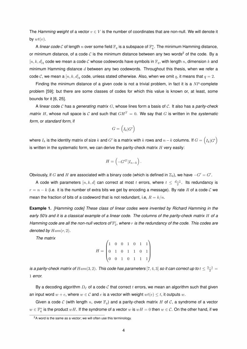
Example 1. [Hamming code] These class of linear codes were invented by Richard Hamming in the
early 50’s and it is a classical example of a linear code. The columns of the parity-check matrix H of a
Hamming code are all the non-null vectors of Fr2, where r is the redundancy of the code. This codes are
denoted by Ham(r, 2).
The matrix
H =
1 0 0 1 0 1 1
0 1 0 1 1 0 1
0 0 1 0 1 1 1
is a parity-check matrix of Ham(3, 2). This code has parameters [7, 4, 3] so it can correct up to t ≤ 3−1
2 =
1 error.
By a decoding algorithm DC of a code C that correct t errors, we mean an algorithm such that given
an input word w + e, where w ∈ C and e is a vector with weight wt(e) ≤ t, it outputs w.
Given a code C (with length n, over Fq) and a parity-check matrix H of C, a syndrome of a vector
w ∈ Fnq is the product wH. If the syndrome of a vector w is wH = 0 then w ∈ C. On the other hand, if we
2A word is the same as a vector; we will often use this terminology.
4
compute the syndrome of a vector y = w + e, where w ∈ C and e is an error vector such that wt(e) ≤ t,
we get
yH = (w + e)H = wH + eH = eH.
So, the syndrome can be used for decoding, since the decoding problem is equal to finding the error
vector e such that yH = eH.
Given a code C and a parity matrix H of C, we define SH(s)−1 as the set of words such that have
syndrome s, i.e,
SH(s)−1 = y + C = y + w : yH = s, w ∈ C.
Finding a vector y ∈ SH(s)−1 can be done in polynomial time. But the following problem is known to be
computationally hard.
Problem 2 (Computational Syndrome Vector). Given a code C ∈ Zn2 of dimension k ≤ n, a parity-check
matrix H of C, a syndrome s ∈ Zr2 and t ∈ N, find a word x ∈ Zn2 such that x ∈ SH(s)−1 and x has weight
wt(x) ≤ t.
This problem was proven to be NP -complete for an arbitrary linear code [7]. If we want to minimize
t, then the problem is in NP -hard. Hence, if the parameters are large enough, the problem becomes
infeasible to solve. What this problem tells us is that decoding a corrupted codeword of an arbitrary code
is a non trivial problem.
One of the main goals of coding theory is to find families of codes such that the Computational
Syndrome Vector problem is easy to solve, i.e., is in P (or BPP ). If we can do that efficiently for a
particular family of codes, we have a family of codes for which decoding is efficient. Also, there is no
known quantum algorithm to solve this problem, which makes this problem interesting for post-quantum
cryptography as we will see later on.
2.2 Goppa Codes
In this thesis we are interested in families of codes that we can use in cryptography and one of the
most important family of those codes is the Goppa codes family. They were first presented in [23], and
latter an English version was published in [5]. We will now see what a Goppa code is and what are its
properties.
A Goppa code is a binary error-correcting code that has some interesting properties for cryptography,
namely the number of errors that it can correct and the number of different codes that we can create, for
a fixed length and minimum distance.
Let p ∈ N. A Goppa code is defined by (g, L) where g ∈ F2p [x] is a polynomial of degree t (with
coefficients in F2p and variable x), and without multiple zeros, and L is a sequence L0, ..., Ln−1 ∈ F2p
such that
Li 6= Lj ∧ g(Li) 6= 0 ∀i, j ∈ 0, ..., n− 1,
i.e., all the elements of L must be different from each other and none of them is a root of g. The code is
5
the set
G(g, L) =
w ∈ Zn2 :
n−1∑i=0
wix− Li
= 0 mod g(x)
.
Theorem 3 ([8]). For a giving pair (g, L = L0, . . . , Ln−1), the parity-check matrix of the corresponding
code is very easy to derive. It can be computed in the following way:
H =
1g(L0) . . . 1
g(Ln−1)
L0
g(L0) . . . Ln−1
g(Ln−1)
......
Lt−10
g(L0) . . .Lt−1n−1
g(Ln−1)
.
The ease with which we create different Goppa codes comes from the ease with which we create
different parity-check matrices.
This code has minimum distance greater or equal than 2t+ 1 since it can correct up to t errors (why
it can correct t errors will be explained latter). The dimension of this code is k = n − mt. Using the
Patterson algorithm [45] one can decode a corrupt Goppa codeword easily. The existence of such a
decoding algorithm is what makes Goppa codes useful for applications. A simple example of a Goppa
code is presented in Example 4.
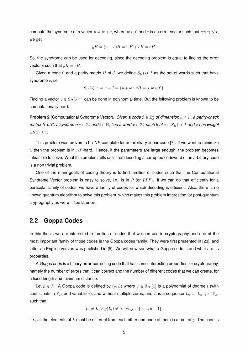
Example 4. Let p = 4 and consider the polynomial f(x) = x4 + x + 1 which is irreducible in F2. We
have that F16 = Z2[x]/〈f(x)〉 is a field. Let α be a solution for the equation x4 + x+ 1 = 0 in F16; α is a
primitive element of F16, i.e., it is a generator for the multiplicative group F∗16 = F16 \ 0.
Now consider the polynomial g(x) = x2 +x+α3 in F16[x] and L = αi : 2 ≤ i ≤ 13 a set of elements
of F16. The code defined by g and l has length 12, minimum distance d ≥ 2t + 1 = 5 and dimension 4.
So its parameters are [12, 4, d] where d ≥ 5.
H =
1g(α2)
1g(α3)
1g(α4)
1g(α5)
1g(α6)
1g(α7)
1g(α8)
1g(α9)
1g(α10)
1g(α11)
1g(α12)
1g(α13)
α2
g(α2)α3
g(α3)α4
g(α4)α5
g(α5)α6
g(α6)α7
g(α7)α8
g(α8)α9
g(α9)α10
g(α10)α11
g(α11)α12
g(α12)α13
g(α13)
=
α3 α9 α4 α α8 α6 α3 α6 α α2 α2 α8
α5 α12 α8 α6 α14 α13 α11 α15 α10 α13 α14 α21
.
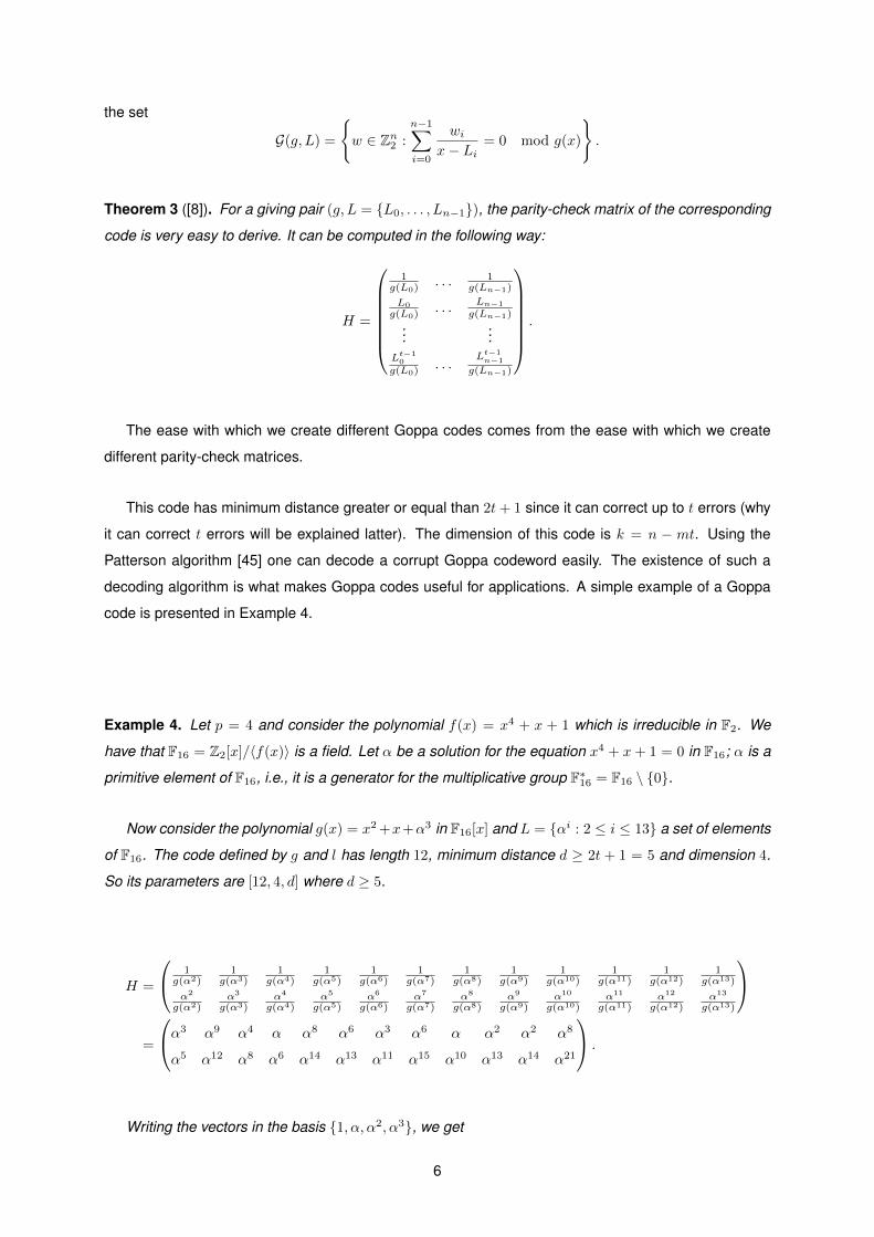
Writing the vectors in the basis 1, α, α2, α3, we get
6
H =
0 0 1 0 1 0 0 0 0 0 0 1
0 1 1 1 0 0 0 0 1 0 0 0
0 0 0 0 1 1 0 1 0 1 1 1
1 1 1 1 0 0 1 0 1 1 1 1
0 1 1 0 1 1 0 1 1 1 1 0
1 1 0 0 0 0 1 0 1 0 0 0
1 1 1 1 0 1 1 0 1 1 0 1
0 1 0 1 1 1 1 0 0 1 1 1
and since GHT = 0, we can compute the generator matrix G, for the code generated by the pair (g, L).
G =
1 1 0 1 1 0 0 0 0 0 0 1
1 1 1 0 1 1 0 1 0 0 1 0
0 1 1 0 1 0 1 0 0 1 0 0
1 1 0 0 0 0 1 0 1 0 0 0
.
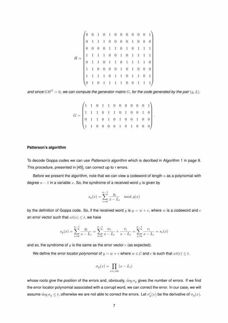
Patterson’s algorithm
To decode Goppa codes we can use Patterson’s algorithm which is decribed in Algorithm 1 in page 9.
This procedure, presented in [45], can correct up to t errors.
Before we present the algorithm, note that we can view a codeword of length n as a polynomial with
degree n− 1 in a variable x. So, the syndrome of a received word y is given by
sy(x) =n−1∑i=0
yix− Li
mod g(x)
by the definition of Goppa code. So, if the received word y is y = w + e, where w is a codeword and e
an error vector such that wt(e) ≤ t, we have
sy(x) =
n−1∑i=0
yix− Li
=
n−1∑i=0
wix− Li
+ei
x− Li=
n−1∑i=0
eix− Li
= se(x)
and so, the syndrome of y is the same as the error vector e (as expected).
We define the error locator polynomial of y = w + e where w ∈ C and e is such that wt(e) ≤ t.
σy(x) =∏i:ei 6=0
(x− Li)
whose roots give the position of the errors and, obviously, deg σy gives the number of errors. If we find
the error locator polynomial associated with a corrupt word, we can correct the error. In our case, we will
assume deg σy ≤ t, otherwise we are not able to correct the errors. Let σ′y(x) be the derivative of σy(x).
7
We have that:
σ′y(x) =∑i:ei 6=0
∏j:ej 6=0j 6=i
(x− Lj) =∑i:ei 6=0
1
x− Li
∏j:ej 6=0
(x− Lj) = se(x)σy(x).
So, we aim to find σy(x) and σ′y(x) that satisfy the equation se(x)σy(x) = σ′y(x) mod g(x) with deg σy(x) ≤
t and deg σ′y(x) ≤ t− 1.
Recall that (a + b)2 = a2 + b2 in a field with characteristic 2. Since σy is a polynomial defined
over a field with characteristic 2, it can be decomposed in α2(x) + xβ2(x), with deg(α) ≤ bt/2c and
deg β ≤ b t−12 c. Hence, σ′y(x) = β2(x). We have
se(x)σy(x) = σ′y(x)⇔ se(x)(α2(x) + xβ2(x)) = β2(x)⇔ α(x) = β(x)d(x) mod g(x)
where d(x)2 = x+ se(x)−1. To efficiently compute d(x), we have the following lemma.
Lemma 5 ([48]). Let x + s−1e (x) = t20(x) + xt21(x) ∈ F2p [x] /〈g(x)〉 and g(x) = h2
0(x) + xh21(x). Let
d(x) = t0(x) + h0(x)h−11 (x)t1(x). Then d(x) =
√x+ s−1
e (x).
There is an algorithm to find such α and β (a variant of Extended Euclidean algorithm [45], noting
that α(x) = β(x)d(x) + g(x)k(x) for some polynomial k(x)), and then we can compute σy(x) and find its
zeros (by checking for which of the Li we have σy(Li) = 0). By decomposing
σy(x) =∏i:ei 6=0
(x− Li)
we can get the non-null coordinates of the error vector and thus correct the received corrupt word.
If the code is defined by a polynomial g with coefficients over F2p such that deg g = t and by a
sequence of numbers L with size n, then this algorithm runs in time O(n.t.p2) [10, 18].
2.3 LDPC Codes
Low-Density Parity-Check (LDPC) codes form a class of linear codes that are obtained from sparse
bipartite graphs. Let X be a bipartite graph; the left nodes of X are called the message nodes (or
variable nodes) and the right nodes are called the check nodes (or constraint nodes). We contruct an
LDPC from X in the following way: given a word w, we associate each left vertex of the graph with each
bit of w; w is a codeword if, for all check nodes, the sum of the neighbor bits (the bits associated with
neighbor nodes) is zero.
In matrix terms, the parity-check matrix H is the adjacency matrix of X. Since X is a sparse graph,
H is a sparse matrix. As usual, the code is defined by the set of words w such that wH = 0.
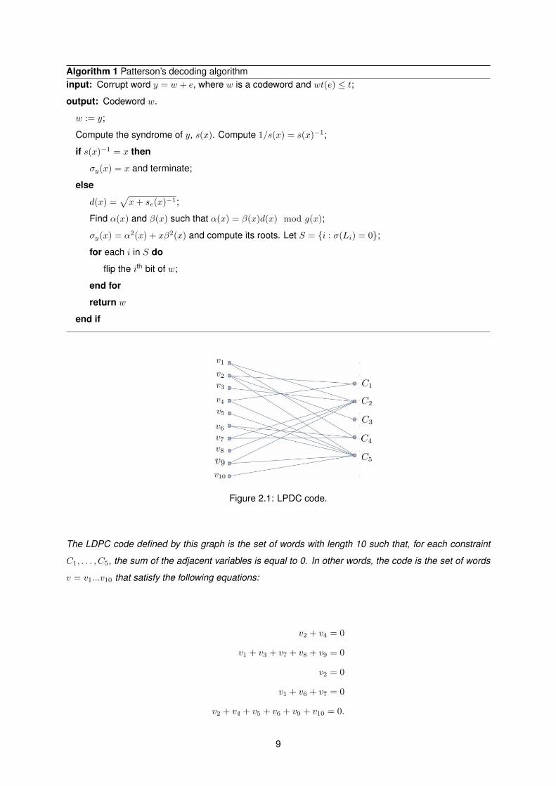
Example 6. Consider the graph presented in Figure 2.1.
The vertices on the left side are called variables, denoted by v1, . . . , v10. The vertices on the right
side are called constraints, denoted by C1, . . . , C5. We associate each variable with a bit of a word.
8
Algorithm 1 Patterson’s decoding algorithminput: Corrupt word y = w + e, where w is a codeword and wt(e) ≤ t;
output: Codeword w.
w := y;
Compute the syndrome of y, s(x). Compute 1/s(x) = s(x)−1;
if s(x)−1 = x then
σy(x) = x and terminate;
else
d(x) =√x+ se(x)−1;
Find α(x) and β(x) such that α(x) = β(x)d(x) mod g(x);
σy(x) = α2(x) + xβ2(x) and compute its roots. Let S = i : σ(Li) = 0;
for each i in S do
flip the ith bit of w;
end for
return w
end if
Figure 2.1: LPDC code.
The LDPC code defined by this graph is the set of words with length 10 such that, for each constraint
C1, . . . , C5, the sum of the adjacent variables is equal to 0. In other words, the code is the set of words
v = v1...v10 that satisfy the following equations:
v2 + v4 = 0
v1 + v3 + v7 + v8 + v9 = 0
v2 = 0
v1 + v6 + v7 = 0
v2 + v4 + v5 + v6 + v9 + v10 = 0.
9
The parity-check matrix is
H =
0 0 0 0 0 0 1 0 1 0
1 1 0 0 1 1 1 0 1 0
0 0 0 0 0 0 0 0 1 0
0 0 0 1 1 0 0 0 0 1
0 1 1 1 0 0 0 1 0 1
,
i.e., it is the adjacency matrix of the graph. Equivalently, we can define the code as the set of words w
such that wH = 0.
The great advantage of LDPC codes is their decoding algorithm. These codes can be decoded using
the so-called belief propagation techniques which make them extremely efficient [30, 36, 37, 50] (we will
see latter examples of these techniques).
LDPC codes differ greatly from algebraic geometry codes (like, for example, Goppa codes). For
the later, it can be extremely difficult to find decoding algorithms, since they are constructed using
combinatorial arguments and the decoding is not taken into account when creating the code. On the
other hand, LDPC codes have very easy and fast decoding algorithms, since the decoding is taken into
account when creating the code.
Here, we will take a quick look on a couple of different families of LDPC codes. These families are
the regular LDPC codes and the expander codes. But before we present these families, we will need
some background on graph theory.
Graph Theory
We will begin with some basic definitions on graph theory. A graph X of size n is a tuple (V,E), where
V = v1, . . . , vn is the set of vertices and E = (u, v) : u, v ∈ V is the set of edges. The degree of a
vertex is the number of edges that are connected to it.
Definition 7 (Regular graph). A a-regular graph is a graph where each vertex has degree a.
By an (a, d)-regular graph, we mean a bipartite graph where: i) we can divide the vertex set into two
disjoint sets such that there are no connections between vertices of the same set; and ii) all vertices in
one set have degree a and all vertices in the other set have degree d.
Definition 8 (Cayley graph). Let G be a group and S a generating set of G. The Cayley graph X =
X(G,S) is the graph where each element g ∈ G is assigned a vertex and the edge set E of X is formed
by pairs (g, gs) for all g ∈ G and s ∈ S.
Definition 9 (Edge-vertex incidence graph). Let X be a graph. The edge-vertex incidence graph of X
is a bipartite graph with vertex set V ′ = E ∪ V and edge set E′ = (e, v) ∈ E × V : v is an endpoint of
e.
10
By a factor expansion δ we mean that, for every subset of vertices S ⊂ V with at most a fixed number
of vertices (i.e., |S| ≤ n for some n ∈ N), the number of adjacent vertices of the elements of S is at least
δ|S|.
Definition 10 (Expander graph). A (a, d, ε, δ) expander graph is a (a, d)-regular graph, where V is the
set of vertices with degree a, such that every S ⊂ V expands by a factor of at least δ, where S has at
most an ε fraction of the vertices with degree a.
Expander graphs are sparse graphs that each small set of vertices have a lot of adjacency vertices.
The existence of these graphs was proven using probabilistic methods [27]. In fact, if we generate a
random (a, d)-regular graph following simple heuristics, we will most likely get an expander graph [58].
Also, there is a deterministic way to construct expander graphs [33] which we will analyse.
There is a relation between expander graphs and the first and second largest eigenvalue (in absolute
value) of the adjacency matrix of the graph [2]: the greater the difference between the first and the
second eigenvalues, the greater the expansion factor of the graph. So now, we will study graphs in
which this difference is maximal.
Let us now assume that X is a connected d-regular graph of n vertices. It is known that its adjacency
matrix has eigenvalues λ0 > λ1 ≥ · · · ≥ λn−1, where λ0 = d and |λj | ≤ d [33]. From now on we will
define λ(X) = maxi |λi| such that |λi| 6= d.
Definition 11 (Ramanujan graph [33]). A graph X is called a Ramanujan graph if λ(X) ≤ 2√d− 1.
Asymptotically, this bound is the smallest possible value for λ(X) [2], since it is proven that
limn→∞
λ(X) ≥ 2√d− 1.
So, for a Ramanujan graph, when the number of vertices n is great enough, the equality holds. And
since the difference between the first and the second eigenvalues will be maximal, these graphs will
have good expander factors (because of the relations between this difference and the expander factors
referred above).
We need to introduce one last notion before we present the algorithm to create explicit Ramanujan
graphs and that is the notion of Projective Linear Group and Projective Special Linear Group.
Definition 12 (Projective Linear Group). Let V be a vector space. We define the Projective Linear Group
PGLn(V ) := GLn(V )/Zn(V )
where GLn(V ) is the General Linear Group3 of degree n and Zn(V ) ≤ GLn(V ) its center.4 Identically,
we define the Projective Special Linear Group PSLn(V ) = SLn(V )/SZn(V ) where SLn(V ) is the spe-
cial linear group of size n and SZn(V ) ≤ SLn(V ) its center. Recall that SLn(V ) is a subgroup of GLn(V )
formed by the matrices whose determinant is 1.
3The group of invertible matrices.4The center of a group is the set of elements that commute with all other elements in the group.
11
For our purpose we are only interested in the case where n = 2 and V = Zq, for some prime number
q.
The center of GL2(Zq) is the subgroup Z2(Zq) formed by the scalar matrices (the matrices that are
a multiple of the identity).
By definition, we have that two elements of GL2(Zq) belong to the same equivalence class in
PGL2(Zq) if they differ by multiplication of a scalar in Zq. In other words, for some α ∈ Z∗q and
A,B ∈ GL2(Zq)
A ∼ B ⇐⇒ A = αB.
Proposition 13. The order of PGL2(Zq) is (q2 − 1)q. The order of PSL2(Zq) is (q2 − 1)q/2.
Proof. To derive the order of the group PGL2(Zq), we use the Lagrange theorem which tells us that the
order of the quotient group G/H is the order of G divided by the order of H, for the finite case. So, we
have that the order of GL2(Zq) is (q2 − 1)(q2 − q) which corresponds to choose a vector v 6= 0 (and we
have q2 − 1 choices for that) and then choose another vector that is not a multiple of v (and we have
q2 − q choices for that). On the other hand, we have that the order of Zn(Zq) is q − 1. So, we conclude
that the order of PGL2(Zq) is (q2 − 1)q.
To derive the order of the group
PSL2(Zq) = SL2(Zq)/SZ2(Zq)
we will use again Lagrange theorem. The order of SL2(Zq) can be computed noting that the homomor-
phism
φ : GL2(Zq)→ F∗q
that gives the determinant of the matrix is surjective and that its kernel is SL2(Zq); by the first isomor-
phism theorem5 and Lagrange theorem we have that
|SL2(Zq)| =|GL2(Zq)||F∗q |
=(q2 − 1)(q2 − q)
q − 1.
To compute the order of SZ2(Zq) note that this group is the intersection between SL2(Zp) and Z2(Z2).
So, an element in SZ2(Zq) is a scalar matrix, since all the matrices in Z2(Z2) are scalar ones. Let A be
a scalar matrix of size 2, then A = λI where I is the identity matrix and λ ∈ Zp. The determinant of A is
λ2. The equation x2 = 1 in Zp has only two solutions in Zp (since p is prime) so the order of SZ2(Zq) is
2.
We conclude that
|PSL2(Z2)| = |SL2(Zq)||SZ2(Zq)|
=(q2 − 1)q
2.
5Recall that if φ : A → B is a surjective homomorphism, then A/Ker(φ) ∼= B. This result is called the first isomorphismtheorem.
12
Construction of Ramanujan graphs
Algorithm 2 describes the construction of explicit Ramanujan graphs and it was first presented in [33].
Algorithm 2 Construction of Ramanujan GraphsChoose p, q primes s.t. p 6= q and p, q = 1 mod 4. Choose i ∈ Z s.t. i2 = −1 mod q;
Compute the p+ 1 possible solutions α = (a0, a1, a2, a3) of p = a20 + a2
1 + a22 + a2
3 where a0 > 0 is odd
and a1, a2, a3 are even;
Use these solutions α = (a0, a1, a2, a3) to construct the set
S =
a0 + i.a1 a2 + ia3
−a2 + ia3 a0 − ia1
: α = (a0, a1, a2, a3)
∈ PGL2(Zq);
if(pq
)= 1 then
Form the Cayley Graph X(G,S) where G = PSL2(Zq);
else(pq
)= −1
Form the Cayley Graph X(G,S) where G = PGL2(Zq);
end if
Here,(pq
)denotes the Jacobi symbol, which is defined as
(pq
)=
0 if p = 0
1 if there is x s.t. p = x2 mod q
−1 otherwise
.
This algorithm gives us a (p+ 1)-regular graph of size n = q(q2− 1), if(pq
)= −1, or n = q(q2− 1)/2,
if(pq
)= 1.
In the case where(pq
)= −1, the graph obtained is also bipartite (between the subgroup PSL2(Zq)
and its complement).
Theorem 14 ([33]). The graph given by Algorithm 2 is a (p+ 1)-regular Ramanujan graph.
Example 15. Let us consider a Ramanujan graph built using Algorithm 2 with p = 13 and q = 5. Since
the Jacobi symbol(
135
)is equal to −1, this graph has 5(52 − 1) = 120 vertices. It is a (14)-regular
graph and it is bipartite. In Figure 2.2 we can see a representation of this graph, implemented using
Mathematica.
Regular LDPC codes
Regular LDPC codes are a subclass LDPC codes in which the graph associated with the code is a
(a, d)-regular bipartite graph, where all the variables nodes have degree a and all the contraints nodes
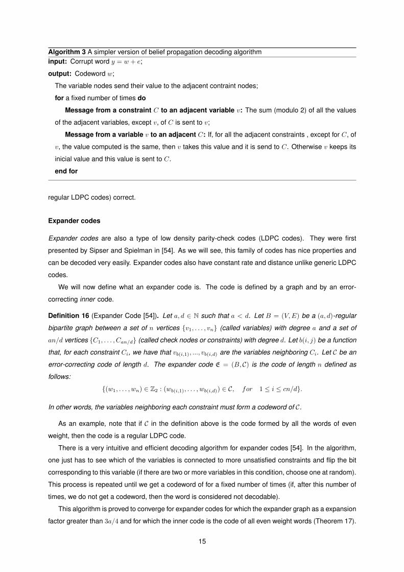
have degree d. They were first presented by Gallager along with a decoding algorithm [22]. Figure 2.3
13
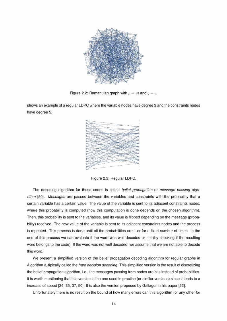
Figure 2.2: Ramanujan graph with p = 13 and q = 5.
shows an example of a regular LDPC where the variable nodes have degree 3 and the constraints nodes
have degree 5.
Figure 2.3: Regular LDPC.
The decoding algorithm for these codes is called belief propagation or message passing algo-
rithm [50]. Messages are passed between the variables and constraints with the probability that a
certain variable has a certain value. The value of the variable is sent to its adjacent constraints nodes,
where this probability is computed (how this computation is done depends on the chosen algorithm).
Then, this probability is sent to the variables, and its value is flipped depending on the message (proba-
bility) received. The new value of the variable is sent to its adjacent constraints nodes and the process
is repeated. This process is done until all the probabilities are 1 or for a fixed number of times. In the
end of this process we can evaluate if the word was well decoded or not (by checking if the resulting
word belongs to the code). If the word was not well decoded, we assume that we are not able to decode
this word.
We present a simplified version of the belief propagation decoding algorithm for regular graphs in
Algorithm 3, tipically called the hard decision decoding. This simplified version is the result of discretizing
the belief propagation algorithm, i.e., the messages passing from nodes are bits instead of probabilities.
It is worth mentioning that this version is the one used in practice (or similar versions) since it leads to a
increase of speed [34, 35, 37, 50]. It is also the version proposed by Gallager in his paper [22].
Unfortunately there is no result on the bound of how many errors can this algorithm (or any other for
14
Algorithm 3 A simpler version of belief propagation decoding algorithminput: Corrupt word y = w + e;
output: Codeword w;
The variable nodes send their value to the adjacent contraint nodes;
for a fixed number of times do
Message from a constraint C to an adjacent variable v: The sum (modulo 2) of all the values
of the adjacent variables, except v, of C is sent to v;
Message from a variable v to an adjacent C: If, for all the adjacent constraints , except for C, of
v, the value computed is the same, then v takes this value and it is send to C. Otherwise v keeps its
inicial value and this value is sent to C.
end for
regular LDPC codes) correct.
Expander codes
Expander codes are also a type of low density parity-check codes (LDPC codes). They were first
presented by Sipser and Spielman in [54]. As we will see, this family of codes has nice properties and
can be decoded very easily. Expander codes also have constant rate and distance unlike generic LDPC
codes.
We will now define what an expander code is. The code is defined by a graph and by an error-
correcting inner code.
Definition 16 (Expander Code [54]). Let a, d ∈ N such that a < d. Let B = (V,E) be a (a, d)-regular
bipartite graph between a set of n vertices v1, . . . , vn (called variables) with degree a and a set of
an/d vertices C1, . . . , Can/d (called check nodes or constraints) with degree d. Let b(i, j) be a function
that, for each constraint Ci, we have that vb(i,1), ..., vb(i,d) are the variables neighboring Ci. Let C be an
error-correcting code of length d. The expander code E = (B, C) is the code of length n defined as
follows:
(w1, . . . , wn) ∈ Z2 : (wb(i,1), . . . , wb(i,d)) ∈ C, for 1 ≤ i ≤ cn/d.
In other words, the variables neighboring each constraint must form a codeword of C.
As an example, note that if C in the definition above is the code formed by all the words of even
weight, then the code is a regular LDPC code.
There is a very intuitive and efficient decoding algorithm for expander codes [54]. In the algorithm,
one just has to see which of the variables is connected to more unsatisfied constraints and flip the bit
corresponding to this variable (if there are two or more variables in this condition, choose one at random).
This process is repeated until we get a codeword of for a fixed number of times (if, after this number of
times, we do not get a codeword, then the word is considered not decodable).
This algorithm is proved to converge for expander codes for which the expander graph as a expansion
factor greater than 3a/4 and for which the inner code is the code of all even weight words (Theorem 17).
15
This algorithm can also be used for regular LDPC codes that are not expander, although convergence
is not guaranteed [37].
Note that the algorithm runs in polynomial time and it is extremely fast, as it only involves bit flipping
operations.
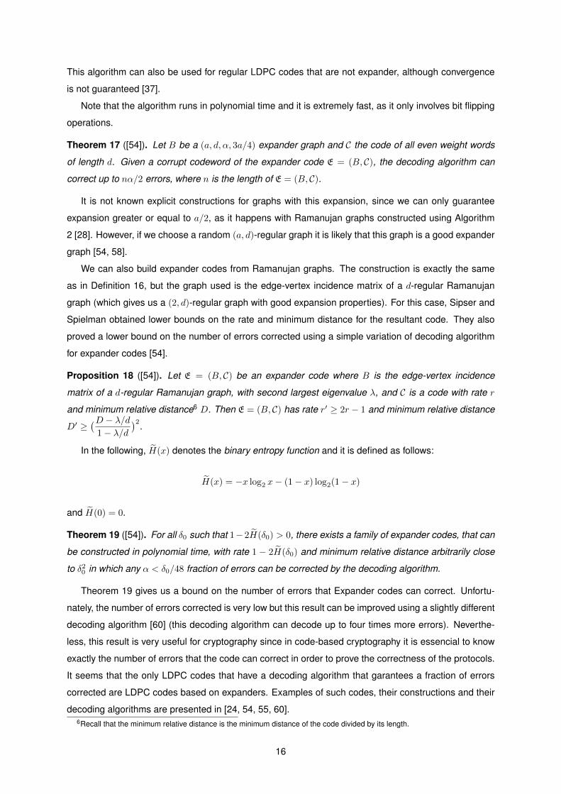
Theorem 17 ([54]). Let B be a (a, d, α, 3a/4) expander graph and C the code of all even weight words
of length d. Given a corrupt codeword of the expander code E = (B, C), the decoding algorithm can
correct up to nα/2 errors, where n is the length of E = (B, C).
It is not known explicit constructions for graphs with this expansion, since we can only guarantee
expansion greater or equal to a/2, as it happens with Ramanujan graphs constructed using Algorithm
2 [28]. However, if we choose a random (a, d)-regular graph it is likely that this graph is a good expander
graph [54, 58].
We can also build expander codes from Ramanujan graphs. The construction is exactly the same
as in Definition 16, but the graph used is the edge-vertex incidence matrix of a d-regular Ramanujan
graph (which gives us a (2, d)-regular graph with good expansion properties). For this case, Sipser and
Spielman obtained lower bounds on the rate and minimum distance for the resultant code. They also
proved a lower bound on the number of errors corrected using a simple variation of decoding algorithm
for expander codes [54].
Proposition 18 ([54]). Let E = (B, C) be an expander code where B is the edge-vertex incidence
matrix of a d-regular Ramanujan graph, with second largest eigenvalue λ, and C is a code with rate r
and minimum relative distance6 D. Then E = (B, C) has rate r′ ≥ 2r − 1 and minimum relative distance
D′ ≥(D − λ/d
1− λ/d)2.
In the following, H(x) denotes the binary entropy function and it is defined as follows:
H(x) = −x log2 x− (1− x) log2(1− x)
and H(0) = 0.
Theorem 19 ([54]). For all δ0 such that 1−2H(δ0) > 0, there exists a family of expander codes, that can
be constructed in polynomial time, with rate 1 − 2H(δ0) and minimum relative distance arbitrarily close
to δ20 in which any α < δ0/48 fraction of errors can be corrected by the decoding algorithm.
Theorem 19 gives us a bound on the number of errors that Expander codes can correct. Unfortu-
nately, the number of errors corrected is very low but this result can be improved using a slightly different
decoding algorithm [60] (this decoding algorithm can decode up to four times more errors). Neverthe-
less, this result is very useful for cryptography since in code-based cryptography it is essencial to know
exactly the number of errors that the code can correct in order to prove the correctness of the protocols.
It seems that the only LDPC codes that have a decoding algorithm that garantees a fraction of errors
corrected are LDPC codes based on expanders. Examples of such codes, their constructions and their
decoding algorithms are presented in [24, 54, 55, 60].6Recall that the minimum relative distance is the minimum distance of the code divided by its length.
16
Chapter 3
Public-key encryption scheme
In this chapter we will analyze public-key encryption schemes and some security notions regarding
them. We will begin by defining what a public-key encryption scheme is. In Section 3.2, we continue
our analysis by introducing two important security notions: (in)distinguishability, which is the ability of
distinguish different ciphertexts, and malleability, which is the ability of creating new ciphertexts from a
known ciphertext. Also, we give the relations between those security notions. Plaintext awareness is a
security notion that is introduced in Section 3.3, where we also present an important result that links this
notion with the others introduced before. Finally, we will end this chapter by giving a generic technique,
the Fujisaki-Okamoto generic conversion, to achieve some of the security notions. This technique is
relevant because it can be applied to any public-key encryption scheme, provided that some conditions
are verified.
3.1 Basic notions
Public-key encryption allows for two parties to communicate privately. Unlike the symmetric setting,
where the two parties need to share a secret-key, in public-key encryption schemes each of the parties
creates a pair of public and secret keys. The public-key is public so that anyone can encrypt messages.
The secret-key is kept private by the owner of the key so that no one else can decrypt messages. We
begin this chapter with a simple definition. In this definition and throughout this thesis, when we say
that some value is chosen randomly, we mean that it is chosen accordingly to a uniform distribution.
When a vector or string is chosen randomly, we mean that each bit is chosen accordingly to a uniform
distribution.
Definition 20 (Public-key cryptosystem). A public-key cryptosystem, or public-key encryption scheme,
Π = (K, E ,D) is composed by three algorithms:
Key creation is a probabilistic polynomial-time algorithm K that receives as input 1k, where k is
a security parameter, and outputs a pair K(1k) = (pk, sk) where pk is the public-key and sk is the
secret-key (or private-key).
Encryption is a probabilistic polynomial-time algorithm E that receives as input a public-key pk and
17
a message to encrypt m, and a string of random coins r, and outputs a ciphertext E(pk,m; k) = c.
Informally, r represents the randomness of the cryptosystem. Throughout this thesis, if we omit r it
means that these coins were chosen randomly.
Decryption is a deterministic polynomial-time algorithm D that receives as input a ciphertext c and
a secret-key sk, and outputs a message D(sk, c) = m, if c is a valid ciphertext; it halts otherwise.
A Public-Key Cryptosystem (PKC) also has to have two more properties: i) Correctness, which
means that a valid ciphertext should be uniquely decrypted to a message using a valid secret-key, i.e.,
D[E(pk,m; r), sk] = m
for every pair (pk, sk) generated by K. And ii) security which means that it should be computationally
hard to recover the message from its ciphertext without the secret-key.
Before we proceed, let us define hash function and cryptographic hash function.
Definition 21 (Hash function). A hash function h is a function that takes as input a string x of arbitrary
size and maps it to a string of a fixed size. We will often call hash value of x to the output of a hash
function given x as input.
Definition 22 (Cryptographic hash function). A cryptographic hash function H is a hash function that
has the following properties:
• It is hard to find collisions, i.e., it is hard to find two strings x and y such that H(x) = H(y);
• It is hard to invert, i.e., given the hash h it is hard to find x such that H(x) = h;
• It is a honest function, i.e., the output size is polynomially bounded by the size of the input.
A cryptographic hash function is a hash function that has an unpredictable behaviour. Hash functions
and, in particular cryptographic hash functions, have a lot of application in cryptography, as we will see.
In the rest of the chapter, we will focus our attention on security notions for public-key encryption
schemes.
3.2 Security Notions
In this section, we will present two important security notions: indistinguishability and non-malleability.
First, we need to define the models and assumptions with which we are going to work with. We will
consider two models of security: the standard model and the random oracle model.
Definition 23 (Standard model). The standard model is a model of security in which the adversary is
limited by the computational time and space available.
Definition 24 (Random oracle). The random oracle model is a model similar to the standard model but
where we assume the existence of an oracle that is an ideal hash H (by an ideal hash we mean a hash
function that returns truly uniformly random numbers for a new query and returns the same value for the
same query).
18
The random oracle simulates cryptographic hash functions and assumes that they have a completely
random behaviour. This is a theoretical model which is very useful to establish security proofs. The
problem is that random oracles are not realistic in the sense that there is no theoretical or empirical
proof that such an oracle exists. In practice, the function used as a random oracle will not behave as a
truly random oracle. Nevertheless, a proof in the random oracle gives us some guaranty and some hope
that it could be used in practice. In other words: a proof in the random oracle is better than no proof at
all.
3.2.1 Indistinguishability
A Public-Key Cryptosystem is indistinguishable if, given two messages and the encryption of one of
them, an adversary is not able to tell which of the messages was encrypted. More precisely, given this
scenario (where one of the messages is encrypted and it is asked to the adversary to tell which one
was), the adversary has a negligible probability of guessing it right. There are three different notions
of indistinguishability: indistinguishability under chosen-plaintext attack (IND-CPA), indistinguishability
under chosen-ciphertext attack (IND-CCA) and indistinguishability under adaptive chosen-ciphertext
attack (IND-CCA2).
In the following, let Π = (K, E ,D) be a Public-Key Cryptosystem and let A be an probabilistic
polynomial-time adversary and C a probabilistic polynomial-time challenger. Suppose that the chal-
lenger C generates a pair of keys (pk, sk) = K(1k) where k is the security parameter of Π. C publishes
pk and keeps sk as a secret.
IND-CPA
By an IND-CPA secure cryptosystem, we mean a cryptosystem for which the adversary A has a negli-
gible probability to win the following game:
1. A can do an arbitrary polynomial number of encryptions;
2. At one point, A submits two different messages m0 and m1 to C;
3. C chooses at random a bit b ∈ 0, 1 and sends the challenge-ciphertext c = E(pk,mb), the
encryption of mb, to A;
4. Again, A can do an arbitrary polynomial number of encryptions;
5. A outputs b, a guess of b.
A wins the game if he can guess correctly the bit b.
INC-CCA
By an IND-CCA secure cryptosystem we mean a cryptosystem for which the adversary A has a negligi-
ble probability to win the following game:
19
1. A can do an arbitrary polynomial number of encryptions and calls to a decryption oracle;
2. At one point, A submits two different messages m0 and m1 to C;
3. C chooses at random a bit b ∈ 0, 1 and sends the challenge-ciphertext c = E(pk,mb), the
encryption of mb, to A;
4. Again, A can do an arbitrary polynomial number of encryptions;
5. A outputs b, a guess of b.
A wins the game if he can guess correctly the bit b.
IND-CCA2
By an IND-CCA2 secure cryptosystem we mean a cryptosystem for which the adversary A has a negli-
gible probability to win the previous game, with the difference that in Step 4, the adversary A can also
do a polynomial number of calls to the decription oracle, with the condition that he can not ask for the
decryption of c.
For a given public-key encryption scheme Π, we formally define the advantage of the adversary A
for any of these games in the following way:
AdvΠ,Aind−aaa(k) = 2.P r(b = b)− 1
where aaa ∈ cpa, cca, cca2. The advantage measures the adversary’s chances of winning the game.
Obviously, the strongest property is the IND-CCA2 property: if a cryptosystem is IND-CCA2 then it
is IND-CCA; and if it is IND-CCA then it is IND-CPA.
Note that if the encryption algorithm of public-key cryptosystem Π is deterministic, then Π is not IND-
CPA secure: for an adversary to find the bit b given the challenge-ciphertext, it just has to encrypt m0
and m1 before hand and check which encryption is equal to the challenge-ciphertext.
3.2.2 Non-malleability
Another important security property is non-malleability . A cryptosystem that is non-malleable prevents
an adversary from creating valid ciphertexts from another ciphertext. Malleability is generally considered
an undesirable property for a cryptosystem as it threatens message integrity (although, in some cases,
this is exactly what we are looking for, as in homomorphic encryption). As in indistinguishability, we
can define 3 levels of non-malleable security: non-malleability under chosen-plaintext attack (NM-CPA),
non-malleability under chosen-ciphertext attack (NM-CCA) and non-malleability under adaptive chosen-
ciphertext attack (NM-CCA2). As in indistinguishability, these three levels differ only on the use of
a decryption oracle by the adversary. Similarly to indistinguishability, non-malleability is defined by a
game where the adversary has to build valid ciphertexts that correspond to valid messages given a valid
ciphertext.
20
Once again, let Π = (K, E ,D) be a public-key cryptosystem and let A be an adversary and C a
challenger. Suppose that the challenger C generates a pair of keys (pk, sk) = K(1k) where k is the
security parameter of Π. C publishes pk and keeps sk as a secret.
NM-CPA
By an NM-CPA secure cryptosystem, we mean a cryptosystem for which the adversary A has a negligi-
ble probability to win the following game:
1. A can do an arbitrary polynomial number encryptions;
2. A outputs a message space M;
3. C chooses a message m from M at random and encrypts it. He sends c = E(pk,m) to A;
4. Given c, A outputs (R, c), where R is a relation and c is a vector (c1, . . . , ck) for some k ∈ N. Here
c is a guess of ciphertexts such that their decryption is related to m by the relation R.
NM-CCA
By an NM-CCA secure cryptosystem we mean a cryptosystem for which the adversaryA has a negligible
probability to win the following game:
1. A can do an arbitrary polynomial number encryptions and calls to a decryption oracle;
2. A outputs a message space M;
3. C chooses a message m from M at random and encrypts it. He sends c = E(pk,m) to A;
4. A outputs (R, c).
NM-CCA2
By an NM-CCA2 secure cryptosystem we mean a cryptosystem for which the adversary A has a negligi-
ble probability to win the previous game, with the difference that, before outputting (R, c), the adversary
A is given access to a decryption oracle that she can query a polynomial number of times.
For a given public-key encryption scheme Π, we define the advantage of the adversary A for any of
these games in the following way:
AdvΠ,Anm−aaa(k) = Pr [m = D(sk, c) : c /∈ c∧ ⊥/∈ m ∧R(m, m)]−Pr [m = D(sk, c) : c /∈ c∧ ⊥/∈ m ∧R(m′, m)]
where aaa ∈ cpa, cca, cca2 and m′ ∈M such that m 6= m′. To prevent the adversary from winning the
game by giving trivial answers, c can not have the challenge ciphertext and every ciphertext in c must
be a valid one a decrypt to a valid message (we prevent this by letting ⊥/∈ m, where ⊥ is the result of
decrypting an invalid ciphertext).
Again, note that the strongest property is that of NM-CCA2.
21
3.2.3 Relations between security notions
Indistinguishability and non-malleability may seem two very different concepts but, in fact, there are
relations among them. These relations were proved by Belare et al. in [3]. We will present some of the
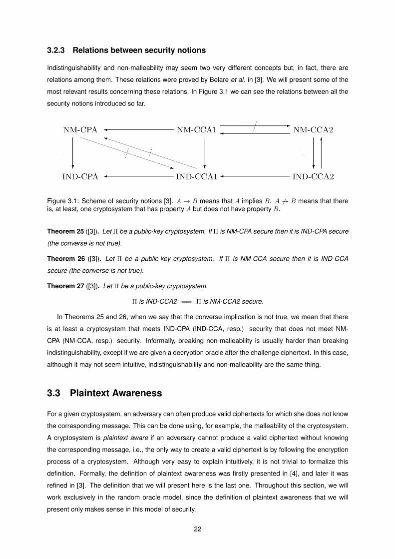
most relevant results concerning these relations. In Figure 3.1 we can see the relations between all the
security notions introduced so far.
Figure 3.1: Scheme of security notions [3]. A → B means that A implies B. A 6→ B means that thereis, at least, one cryptosystem that has property A but does not have property B.
Theorem 25 ([3]). Let Π be a public-key cryptosystem. If Π is NM-CPA secure then it is IND-CPA secure
(the converse is not true).
Theorem 26 ([3]). Let Π be a public-key cryptosystem. If Π is NM-CCA secure then it is IND-CCA
secure (the converse is not true).
Theorem 27 ([3]). Let Π be a public-key cryptosystem.
Π is IND-CCA2 ⇐⇒ Π is NM-CCA2 secure.
In Theorems 25 and 26, when we say that the converse implication is not true, we mean that there
is at least a cryptosystem that meets IND-CPA (IND-CCA, resp.) security that does not meet NM-
CPA (NM-CCA, resp.) security. Informally, breaking non-malleability is usually harder than breaking
indistinguishability, except if we are given a decryption oracle after the challenge ciphertext. In this case,
although it may not seem intuitive, indistinguishability and non-malleability are the same thing.
3.3 Plaintext Awareness
For a given cryptosystem, an adversary can often produce valid ciphertexts for which she does not know
the corresponding message. This can be done using, for example, the malleability of the cryptosystem.
A cryptosystem is plaintext aware if an adversary cannot produce a valid ciphertext without knowing
the corresponding message, i.e., the only way to create a valid ciphertext is by following the encryption
process of a cryptosystem. Although very easy to explain intuitively, it is not trivial to formalize this
definition. Formally, the definition of plaintext awareness was firstly presented in [4], and later it was
refined in [3]. The definition that we will present here is the last one. Throughout this section, we will
work exclusively in the random oracle model, since the definition of plaintext awareness that we will
present only makes sense in this model of security.
22
Definition 28 (Plaintext Awareness). Let Π = (K, E ,D) be a public-key encryption scheme, A an adver-
sary, H a cryptographic hash function and K an algorithm called the knowledge extractor. Consider the
following game between a challenger C and the adversary A.
• C creates a pair of keys (pk, sk) = K(1k). He publishes pk.
• A has access to the oracle H and to an encryption oracle. She can do a polynomial number
of queries to each oracle. Eventually, she outputs (τ, η, y) where τ = (h1,H1), . . . , (hqH ,Hqh)
is a list of queries h1, . . . , hqH to the H oracle and the corresponding answers H1, . . . ,HqH , η =
y1, . . . , yqE is a list of answers received by A of the queries done to the encryption oracle and
y /∈ η.
• C uses algorithm K, that receives as input (τ, η, y, pk), to try to find the decryption of y.
We define
AdvK,Π,Bpa (k) := Pr[K(τ, η, y, pk) = D(sk, y)].
We say that K is a λ(k)-knowledge extractor if K runs in polynomial time and AdvK,Π,Bpa (k) ≥ λ(k).
If Π is IND-CPA secure and there exists a λ(k)-knowledge extractor K, where 1−λ(k) is a negligible
value, then we say that Π is plaintext aware (PA) secure.
Informally, a knowledge extractor receives a ciphertext and tries to find its decryption using only the
queries made by A and respective answers to the hash oracle and answers from the encryption oracle.
Again, we can relate the concept of plaintext awareness with the security concepts of indistinguisha-
bility and non-malleability. In fact, plaintext awareness is the strongest security property. This means that
if one can only build valid ciphertexts by following the encryption algorithm, then one can not distinguish
ciphertexts.
Theorem 29 ([3]). If a public-key cryptosystem is PA secure then it is IND-CCA2 secure.
As a corollary, we can state that if a public-key cryptosystem is PA secure then it is NM-CCA2 secure.
3.4 Fujisaki-Okamoto IND-CCA2 generic conversion
Unfortunately, IND-CCA2 secure cryptosystems are not easy to construct. But, although most of the
cryptosystems are not IND-CCA2 secure, there are some generic conversions, which we can apply to a
cryptosystem that is not IND-CCA2 secure to obtain a new cryptosystem that is IND-CCA2 secure.
In this thesis we present one of these conversions, the Fujisaki-Okamoto simple IND-CCA2 con-
version [21]. We believe that this is one of the simplest and most efficient conversions of which we
are aware. The conversion aims to build a new IND-CCA2 secure cryptosystem Π = (K, E , D), in the
random oracle model, from an IND-CPA secure cryptosystem Π = (K, E ,D), where K is the key cre-
ation algorithm, E is the encryption algorithm and D is the decryption algorithm. The cryptosystem is
presented in Algorithm 4. Before we take a look at the cryptosystem, we need a small definition.
23
Definition 30 (γ-uniform cryptosystem). Let Π be a public-key cryptosystem. For any message m and
any ciphertext c, we say that Π is γ-uniform if, given a message m and a ciphertext c, the probability of
guessing the encryption coins r at random such that E(pk,m; r) = c is less or equal than γ.
Informally, this value γ measures the randomness that is used in the encryption of a message in the
cryptosystem Π. If the encryption of a certain public-key encryption scheme is completely deterministic,
then γ = 1. For this conversion to work, γ < 1. Recall that if the encryption of a cryptosystem Π is
deterministic, then Π is not IND-CPA secure.
We now present the conversion in Algorithm 4. The idea is very simple: the message concatenated
with a random string1 will determine the random coins used in the encryption proccess. In other words,
they will determine the randomness used in the encryption. When decrypting the ciphertext, one just
has to verify if the encryption of the message using these coins is the received ciphertext; if this does
not happen, then this ciphertext is an invalid one.
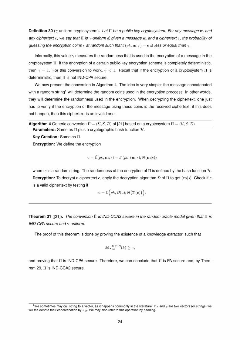
Algorithm 4 Generic conversion Π = (K, E , D) of [21] based on a cryptosystem Π = (K, E ,D)
Parameters: Same as Π plus a cryptographic hash function H.
Key Creation: Same as Π.
Encryption: We define the encryption
c = E(pk,m; s) = E (pk, (m|s);H(m|s))
where s is a random string. The randomness of the encryption of Π is defined by the hash function H.
Decryption: To decrypt a ciphertext c, apply the decryption algorithm D of Π to get (m|s). Check if c
is a valid ciphertext by testing if
c = E(pk,D(c);H
(D(c)
)).
Theorem 31 ([21]). The conversion Π is IND-CCA2 secure in the random oracle model given that Π is
IND-CPA secure and γ-uniform.
The proof of this theorem is done by proving the existence of a knowledge extractor, such that
AdvK,Π,Bpa (k) ≥ γ,
and proving that Π is IND-CPA secure. Therefore, we can conclude that Π is PA secure and, by Theo-
rem 29, Π is IND-CCA2 secure.
1We sometimes may call string to a vector, as it happens commonly in the literature. If x and y are two vectors (or strings) wewill the denote their concatenation by x|y. We may also refer to this operation by padding.
24
Chapter 4
McEliece Cryptosystem
Since Diffie and Hellman introduced the concept of public-key cryptography [15], numerous public-key
cryptosystems (PKC) have been proposed by the cryptographic community. These PKC are based on
various conjectured computational hard problems, the most famous and used in practice being RSA,
based on the integer factoring problem [47], and El Gamal PKC, based on the discrete logarithmic
problem [17]. The situation could be dramatic if one was able to find a practical algorithm that could
solve one of these problems, and thus break the cryptosystems. Unfortunately, no one can say if such
an algorithm will be or will not be found.
In fact, Shor has already found a polynomial-time quantum algorithm that solves the integer factoring
problem and the discrete logarithmic problem [51]. Since it is a quantum algorithm, it cannot yet be
used in practice. But still, several alternative proposals are arising to replace RSA PKC and El Gamal
PKC. These alternatives are based on computational hard problems that were recently presented and
that are conjectured to be unsolvable in polynomial time even by quantum computers. Post-quantum
cryptography deals with cryptographic classical algorithms based on these problems, thus it deals with
cryptographic algorithms that are conjectured to be robust to quantum attacks, i.e., that are in the com-
plexity class BQP . Code-based, lattice-based and multivariate polynomials problems are among these
problems and they are being used for post-quantum cryptography right now [10].
Among these cryptosystems, we have the McEliece cryptosystem proposed by Robert McEliece [39]
which is a code-based cryptosystem. This cryptosystem is one of the oldest public-key cryptosystems
that is still secure and thus it is a very interesting candidate for post-quantum cryptography. Although
there is no security reduction for the McEliece PKC, the extensive cryptoanalysis that it has been subject
over the years has failed to find polynomial-time attacks. This fact has reinforced the conjecture that the
McEliece cryptosystem is not efficiently breakable.
In this chapter we will analyze the McEliece PKC. We will begin by presenting, in Section 4.1 the
cryptosystem along with its dual version, the Niederreiter PKC. In Section 4.2 we will analyze the secu-
rity of the McEliece cryptosystem and we will explore some of its weaknesses. Section 4.3 is where we
analyze the McEliece PKC computational complexity and efficiency, both of them very important aspects
that must be taken into account for practical purposes. In Section 4.4, we will present some known vari-
25
ants that meet some important security properties, like IND-CPA and IND-CCA2. Finally, in Section 4.5,
we will talk on the usage of LDPC codes in the McEliece PKC and its advantages and drawbacks.
4.1 The Cryptosystem
The McEliece PKC was presented by Robert McEliece in [39]. It remains unbreakable and it is also
conjectured to be robust to quantum attacks. The McEliece cryptosystem is described in Algorithm 5.
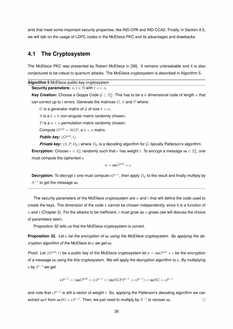
Algorithm 5 McEliece public-key cryptosystemSecurity parameters: n, t ∈ N with t << n.
Key Creation: Choose a Goppa Code G ⊂ Zn2 : This has to be a k dimensional code of length n that
can correct up to t errors. Generate the matrices G, S and P where:
G is a generator matrix of G of size k × n;
S is a k × k non-singular matrix randomly chosen;
P is a n× n permutation matrix randomly chosen;
Compute Gpub = SGP , a k × n matrix.
Public key: (Gpub, t).
Private key: (S, P,DG) where DG is a decoding algorithm for G, tipically Patterson’s algorithm.
Encryption: Choose e ∈ Zn2 randomly such that e has weight t. To encrypt a message m ∈ Zk2 , one
must compute the ciphertext c
c = mGpub + e.
Decryption: To decrypt c one must compute cP−1, then apply DG to the result and finally multiply by
S−1 to get the message m.
The security parameters of the McEliece cryptosystem are n and t that will define the code used to
create the keys. The dimension of the code k cannot be chosen independently, since it is a function of
n and t (Chapter 2). For the attacks to be inefficient, t must grow as n grows (we will discuss the choice
of parameters later).
Proposition 32 tells us that the McEliece cryptosystem is correct.
Proposition 32. Let c be the encryption of m using the McEliece cryptosystem. By applying the de-
cryption algorithm of the McEliece to c we get m.
Proof. Let (Gpub, t) be a public key of the McEliece cryptosystem let c = mGpub + e be the encryption
of a message m using the this cryptosystem. We will apply the decryption algorithm to c. By multiplying
c by P−1 we get
cP−1 = (mGpub + e)P−1 = (mSGPP−1 + eP−1) = mSG+ eP−1
and note that eP−1 is still a vector of weight t. So, applying the Patterson’s decoding algorithm we can
extract mS from mSG+ eP−1. Then, we just need to multiply by S−1 to recover m.
26
A simple example of the Algorithm 5 is presented.
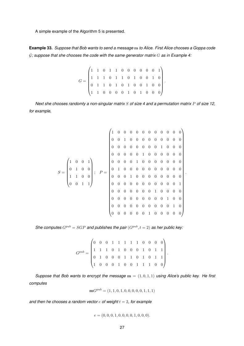
Example 33. Suppose that Bob wants to send a message m to Alice. First Alice chooses a Goppa code
G; suppose that she chooses the code with the same generator matrix G as in Example 4:
G =
1 1 0 1 1 0 0 0 0 0 0 1
1 1 1 0 1 1 0 1 0 0 1 0
0 1 1 0 1 0 1 0 0 1 0 0
1 1 0 0 0 0 1 0 1 0 0 0
.
Next she chooses randomly a non-singular matrix S of size 4 and a permutation matrix P of size 12,
for example,
S =
1 0 0 1
0 1 0 0
1 1 0 0
0 0 1 1
; P =
1 0 0 0 0 0 0 0 0 0 0 0
0 0 1 0 0 0 0 0 0 0 0 0
0 0 0 0 0 0 0 0 1 0 0 0
0 0 0 0 0 1 0 0 0 0 0 0
0 0 0 0 1 0 0 0 0 0 0 0
0 1 0 0 0 0 0 0 0 0 0 0
0 0 0 1 0 0 0 0 0 0 0 0
0 0 0 0 0 0 0 0 0 0 0 1
0 0 0 0 0 0 0 1 0 0 0 0
0 0 0 0 0 0 0 0 0 1 0 0
0 0 0 0 0 0 0 0 0 0 1 0
0 0 0 0 0 0 1 0 0 0 0 0
.
She computes Gpub = SGP and publishes the pair (Gpub, t = 2) as her public key:
Gpub =
0 0 0 1 1 1 1 1 0 0 0 0
1 1 1 0 1 0 0 0 1 0 1 1
0 1 0 0 0 1 1 0 1 0 1 1
1 0 0 0 1 0 0 1 1 1 0 0
.
Suppose that Bob wants to encrypt the message m = (1, 0, 1, 1) using Alice’s public key. He first
computes
mGpub = (1, 1, 0, 1, 0, 0, 0, 0, 0, 1, 1, 1)
and then he chooses a random vector e of weight t = 2, for example
e = (0, 0, 0, 1, 0, 0, 0, 0, 1, 0, 0, 0).
27
He computes
c = mGpub + e = (1, 1, 0, 0, 0, 0, 0, 0, 1, 1, 1, 1)
and sends c to Alice.
For Alice to decrypt the cipher c using her private key, she first computes
cP−1 = (1, 0, 1, 0, 0, 1, 0, 1, 0, 1, 1, 0)
then she applies Patterson’s Algorithm (Algorithm 1 in page 9) to cP−1 to get m′ = (0, 1, 1, 0) and finally
she computes m′S−1 to recover the message m.
4.1.1 The Niederreiter Cryptosystem
The Niederreiter cryptosystem was proposed by Harald Niederreiter in 1986, in [43]. It is very similar
to the McEliece cryptosystem; in fact the Niederreiter cryptosystem is the dual version of the previous
cryptosystem. The main difference is that the message space is the set of errors with weight t of a given
code C and the message is encrypted as a syndrome.
Since this protocol only encrypts words of length n and weight t, we need a function to transform each
word in Zl2 in a word that can be encrypted. Let φn,t : Zl2 → Wn,t, where Wn,t = e ∈ Zn2 : wt(e) = t
and l = blog |Wn,t|c, be that function. An explicit construction for this function can be found in [20] but
we will treat it as a black-box.
Also, and since this cryptosystem is the dual version of the previous one, we will need a different
decoding algorithm. We will call it the syndrome decoding algorithm.
Definition 34. Let C be a code that corrects up to t errors andH its parity-check matrix. Let e be an error
vector with wt(e) ≤ t. A syndrome decoding algorithm SD is an algorithm such that given a syndrome
s = eHT , it outputs e.
Proposition 35. Let C be a code with parameters [n, k, d] that corrects up to t errors. If there is a
decoding algorithm D then there exists a syndrome decoding algorithm SD, and vice versa.
Proof. Let G and H be the generating and parity-check matrix of C, respectively. Let e be a error vector
with wt(e) ≤ t.
Let SD be a syndrome decoding algorithm of C such that for every e ∈ Wn,t we have SD(eHT ) = e.
Given a word mG+e we want to derive a decoding algorithm D such that D(mG+e) = mG. We can do
that in the following way: multiply mG+e by HT to get eHT , then calculate mG = (mG+e)+SD(eHT ).
Now, given a decoding algorithm D we will construct a syndrome decoding algorithm. Given a
syndrome s = eHT , first we need to find a vector e′ such that e′HT = s (this can be done in polynomial-
time, see Chapter 2). We know that e′ − e is a codeword of C, since
(e′ − e)HT = e′HT − eHT = s− s = 0.
28
So e′ = w + e where w is a codeword of C. Then we apply D to e′ to get w and, finally, we can calculate
e = e′ − w.
A description of the Niederreiter PKC is presented in Algorithm 6. Usually, the code used in the
cryptosystem is a Goppa code.
Algorithm 6 Niederreiter public-key cryptosystemSecurity parameters: n, t ∈ N with t << n.
Key Creation: Choose a k dimensional binary code C with length n that can correct up to t errors.
Generate the matrices H, S and P where:
H is a parity-check matrix of C of size (n− k)× k;
S is a k × k non-singular matrix randomly chosen;
P is a n× n permutation matrix randomly chosen.
Compute Hpubk×n = SHP .
Public key: (Hpub, t).
Private key: (S, P, SDC) where SDC is a syndrom decoding algorithm for C.
Encryption: To encrypt m ∈ Zl2, calculate φn,t(m) = e where φn,t is a function that takes a message
in Zl2 and maps it to a vector of length n and weight t. Compute the ciphertext c as
c = e(Hpub)T .
Decryption: To decrypt c, compute c(S−1)T = ePTHT , then apply SDC to get ePT . Finally compute
e = ePT (P−1)T and recover m with m = φ−1n,t(e).
The advantage of using this protocol instead of McEliece cryptosystem is that the keys are much
smaller and the encryption is faster (although the decryption takes more time) [10]. Another advantage
is that it can be used to produce a secure signature scheme [14].
4.2 Security
In this section, we will first talk about the assumptions on which the security of the McEliece cryptosystem
is based. Then we will go through some of the most important attacks on the cryptosystem. Finally, we
will analyze the security parameters of the McEliece and the corresponding security level and key size.
Security of the McEliece
We define the McEliece problem:
Problem 36 (McEliece Problem). Given a a public key pk and a ciphertext c, that was obtained encrypt-
ing a message m using the McEliece cryptosystem with pk, recover the message m.
29
The McEliece cryptosystem, like other cryptosystems, relies on the exhaustive search problem
(which is a computationally hard problem) since we can define the McEliece problem as follows: given
a public key (Gpub, t) and a ciphertext c ∈ Zn2 , find the message m ∈ Zk2 such that wt(mGpub − c) = t.
Obviously, solving the McEliece problem is equivalent to breaking the McEliece cryptosystem. This
can be done in two ways: recovering the message m directly or recovering the secret key from the public
key.
First, we will talk about the security of the message. The security of the message in the McEliece
cryptosystem relies on the hardness of the Computational Syndrome Vector since we can define the
McEliece problem as follow: given an irreducible Goppa code G over Z2 and a ciphertext c, find a vector
e with weight wt(e) ≤ t such that c + e is a permuted codeword of C. So it is obvious that if one
solves the Computational Syndrome Vector problem, then one breaks the cryptosystem (apart from the
permutation). But the problems are not known to equivalent. The reciprocal is not known to be true,
since if one breaks the cryptosystem, one only solves the Computational Syndrome Vector problem for
a certain class of codes, namely, in this case the Goppa codes. But we can choose the parameters of
the code G in such way that the McEliece cryptosystem is as difficult as possible as the Computational
Syndrome Problem. Equivalently, we can say that the McEliece cryptosystem relies on the Learning
with Parity Noise (LPN) problem, a classical problem in learning theory.
Problem 37 (Learning with Parity Noise). Let s (the secret) be a word of length l. Given the pair
(a, 〈s, a〉+ e)
where a ∈ Zl2, 〈s, a〉 denotes the usual inner product of s and a, and e is chosen using the Bernoulli
distribution Bθ with parameter θ ∈ [0, 1/2], find s.
This problem is also conjectured to be hard, and it is often used to argue that the McEliece cryp-
tosystem is hard to break. It is useful, in some circumstances, to use the hardness of this problem for
proofs instead of the hardness of the Computational Syndrome Vector problem, as we will see later.
Another assumption on which the security of the McEliece PKC is based is the difficulty of distinguish
a permuted Goppa code generating matrix from a randomly (uniformly) chosen binary matrix [14].
Problem 38 (Goppa Distinguisher Problem). Given a matrixMk×n, output 1 ifM represents a generating
matrix of a Goppa code and output 0 if M was chosen uniformly at random (i.e., each coordinate of M
was chosen uniformly at random).
Although there is no proof that this problem is NP -complete, it remains unsolvable for a long time and,
thus, it is conjectured to be a hard problem. This does not happen with other classes of codes. Several
attempts of using other codes in the McEliece, with the objective of reducing key size or increasing
efficiency, have turned out failures since all of them almost immediatly reveal their structure and this can
be used to break the cryptosystem [10, 41, 52]. But surprisingly, coding theorists have not found a way
of distinguish Goppa codes generating matrices from random matrices.
30
We conclude that, in the McEliece cryptosystem, the security of the message is based on the Com-
putational Syndrome Vector problem (or, sometimes, on the Learning with Parity Noise problem) and
the security of the public key is based on the Goppa Distinguisher problem. Assuming that the Compu-
tational Syndrome Vector and the Goppa Distinguisher problems are hard, we can conjectured that the
McEliece problem is hard.
Attacks on the McEliece
Several attacks have been found to the McEliece cryptosystem. While some of them can be avoided
just by increasing the security parameters, others are more difficult to prevent since they are based on
the structure of the cryptosystem. In the following, we will use the same notation as in Algorithm 5. We
now present some of these attacks:
• Information set decoding attack: The information set decoding is an algorithm for decoding any
arbitrary code. Although it can be applied to any code, it is not very efficient if the parameters of
the McEliece cryptosystem are chosen properly. But still, this (or variants of it) is the best known
attack. The idea of this attack is to pick a set of coordinates of the ciphertext not affected by the
error vector and this set has to be sufficiently large such that the columns of the public generator
matrix is an invertible matrix. That is, choose K ⊂ 1, . . . n with k elements (k is the dimension of
the code). GpubK , cK and eK are formed by the columns of Gpub, c and e (respectively) in positions
of elements in K. So if eK = 0 and GpubK is invertible then
m = cK(GpubK )−1 = (ck + ek)(GpubK )−1
and the message m can be recovered. This process takes at least Ω(n2) operations (to multiply
matrices, we need at least to write them) and to be successful, it needs to be iterated(nk
)/(n−tk
)times. Thus the complexity1 of this attack is
Ω
(n2
(nk
)(n−tk
)) .So, simply by enlarging the parameters, the attack becomes infeasible.
The best known attacks to the McEliece PKC are variants and optimizations of this algorithm, like
Stern’s attack [56].
• Quantum attack: The best known quantum attack to the McEliece cryptosystem is the quantum
set decoding attack, which is based on Grover’s algorithm [9]. The main idea is to use Grover’s
algorithm to increase the speed of the information set decoding attack. This approach increases
1In this thesis, we present lower bounds on the complexity of the attacks (Big-Omega notation), instead of the usual upper-bounds used to analyze the complexity of algorithms (Big-O notation).
31
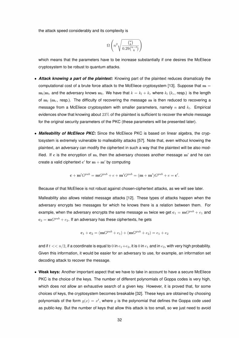
the attack speed considerably and its complexity is
Ω
(n2
√ (nk
)0.29
(n−tk
))
which means that the parameters have to be increase substantially if one desires the McEliece
cryptosystem to be robust to quantum attacks.
• Attack knowing a part of the plaintext: Knowing part of the plaintext reduces dramaticaly the
computational cost of a brute force attack to the McEliece cryptosystem [13]. Suppose that m =
ml|mr and the adversary knows ml. We have that k = kl + kr where kl (kr, resp.) is the length
of ml (mr, resp.). The difficulty of recovering the message m is then reduced to recovering a
message from a McEliece cryptosystem with smaller parameters, namely n and kl. Empirical
evidences show that knowing about 23% of the plaintext is sufficient to recover the whole message
for the original security parameters of the PKC (these parameters will be presented later).
• Malleability of McEliece PKC: Since the McEliece PKC is based on linear algebra, the cryp-
tosystem is extremely vulnerable to malleability attacks [57]. Note that, even without knowing the
plaintext, an adversary can modify the ciphertext in such a way that the plaintext will be also mod-
ified. If c is the encryption of m, then the adversary chooses another message m′ and he can
create a valid ciphertext c′ for m + m′ by computing
c + m′Gpub = mGpub + e+ m′Gpub = (m + m′)Gpub + e = c′.
Because of that McEliece is not robust against chosen-ciphertext attacks, as we will see later.
Malleability also allows related message attacks [12]. These types of attacks happen when the
adversary encrypts two messages for which he knows there is a relation between them. For
example, when the adversary encrypts the same message m twice we get c1 = mGpub + e1 and
c2 = mGpub + e2. If an adversary has these ciphertexts, he gets
c1 + c2 = (mGpub + e1) + (mGpub + e2) = e1 + e2
and if t << n/2, if a coordinate is equal to 0 in e1+e2, it is 0 in e1 and in e2, with very high probability.
Given this information, it would be easier for an adversary to use, for example, an information set
decoding attack to recover the message.
• Weak keys: Another important aspect that we have to take in account to have a secure McEliece
PKC is the choice of the keys. The number of different polynomials of Goppa codes is very high,
which does not allow an exhaustive search of a given key. However, it is proved that, for some
choices of keys, the cryptosystem becomes breakable [32]. These keys are obtained by choosing
polynomials of the form g(x) = xt, where g is the polynomial that defines the Goppa code used
as public-key. But the number of keys that allow this attack is too small, so we just need to avoid
32
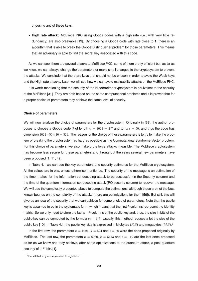
choosing any of these keys.
• High rate attack: McEliece PKC using Goppa codes with a high rate (i.e., with very little re-
dundancy) are also breakable [19]. By choosing a Goppa code with rate close to 1, there is an
algorithm that is able to break the Goppa Distinguisher problem for those parameters. This means
that an adversary is able to find the secret key associated with this code.
As we can see, there are several attacks to McEliece PKC, some of them pretty efficient but, as far as
we know, we can always change the parameters or make small changes to the cryptosystem to prevent
the attacks. We conclude that there are keys that should not be chosen in order to avoid the Weak keys
and the High rate attacks. Later we will see how we can avoid malleability attacks on the McEliece PKC.
It is worth mentioning that the security of the Niederreiter cryptosystem is equivalent to the security
of the McEliece [31]. They are both based on the same computational problems and it is proved that for
a proper choice of parameters they achieve the same level of security.
Choice of parameters
We will now analyse the choice of parameters for the cryptosystem. Originally in [39], the author pro-
poses to choose a Goppa code G of length n = 1024 = 210 and to fix t = 50, and thus the code has
dimension 1024−50×10 = 524. The reason for the choice of these parameters is to try to make the prob-
lem of breaking the cryptosystem as hard as possible as the Computational Syndrome Vector problem.
For this choice of parameters, we also make brute force attacks infeasible. The McEliece cryptosystem
has become less secure for these parameters and throughout the years several new parameters have
been proposed [1, 11, 42].
In Table 4.1 we can see the key parameters and security estimates for the McEliece cryptosystem.
All the values are in bits, unless otherwise mentioned. The security of the message is an estimation of
the time it takes for the information set decoding attack to be successful (in the Security column) and
the time of the quantum information set decoding attack (PQ security column) to recover the message.
We will use the complexity presented above to compute the estimations, although these are not the best
known bounds on the complexity of the attacks (there are optimizations for them [56]). But still, this will
give us an idea of the security that we can achieve for some choice of parameters. Note that the public
key is assumed to be in the systematic form, which means that the first k columns represent the identity
matrix. So we only need to store the last n− k columns of the public-key and, thus, the size in bits of the
public-key can be computed by the formula (n − k)k. Usually, this method reduces a lot the size of the
public key [10]. In Table 4.1, the public key size is expressed in kilobytes (KB) and megabytes (MB).2
In the first row, the parameters n = 1024, k = 524 and t = 50 were the ones proposed originally by
McEliece. The last row, the parameters n = 6960, k = 5413 and t = 119 are the last ones proposed
as far as we know and they achieve, after some optimizations to the quantum attack, a post-quantum
security of 2128 bits [1].
2Recall that a byte is equivalent to eight bits.
33
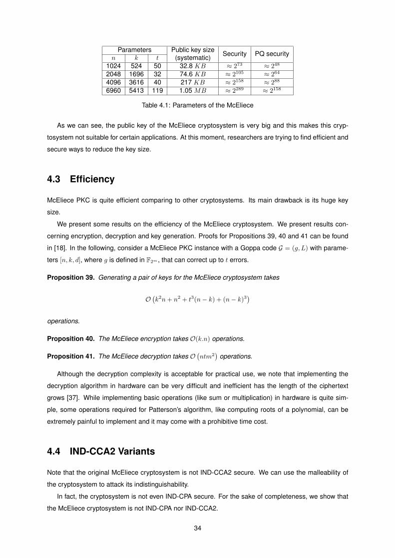
Parameters Public key size(systematic) Security PQ security
n k t1024 524 50 32.8 KB ≈ 273 ≈ 248
2048 1696 32 74.6 KB ≈ 2105 ≈ 264
4096 3616 40 217 KB ≈ 2158 ≈ 288
6960 5413 119 1.05 MB ≈ 2289 ≈ 2158
Table 4.1: Parameters of the McEliece
As we can see, the public key of the McEliece cryptosystem is very big and this makes this cryp-
tosystem not suitable for certain applications. At this moment, researchers are trying to find efficient and
secure ways to reduce the key size.
4.3 Efficiency
McEliece PKC is quite efficient comparing to other cryptosystems. Its main drawback is its huge key
size.
We present some results on the efficiency of the McEliece cryptosystem. We present results con-
cerning encryption, decryption and key generation. Proofs for Propositions 39, 40 and 41 can be found
in [18]. In the following, consider a McEliece PKC instance with a Goppa code G = (g, L) with parame-
ters [n, k, d], where g is defined in F2m , that can correct up to t errors.
Proposition 39. Generating a pair of keys for the McEliece cryptosystem takes
O(k2n+ n2 + t3(n− k) + (n− k)3
)operations.
Proposition 40. The McEliece encryption takes O(k.n) operations.
Proposition 41. The McEliece decryption takes O(ntm2
)operations.
Although the decryption complexity is acceptable for practical use, we note that implementing the
decryption algorithm in hardware can be very difficult and inefficient has the length of the ciphertext
grows [37]. While implementing basic operations (like sum or multiplication) in hardware is quite sim-
ple, some operations required for Patterson’s algorithm, like computing roots of a polynomial, can be
extremely painful to implement and it may come with a prohibitive time cost.
4.4 IND-CCA2 Variants
Note that the original McEliece cryptosystem is not IND-CCA2 secure. We can use the malleability of
the cryptosystem to attack its indistinguishability.
In fact, the cryptosystem is not even IND-CPA secure. For the sake of completeness, we show that
the McEliece cryptosystem is not IND-CPA nor IND-CCA2.
34
Proposition 42. The original McEliece cryptosystem is not IND-CPA secure.
Proof. To prove that the original McEliece is not IND-CPA secure, we will build an adversary A that has
a non-negligible probability of winning the IND-CPA game.
A follows this simple strategy: when A receives the challenge-ciphertext c, she computes
e0 = c + m0Gpub and e1 = c + m1G
pub.
Note that
e0 = c + m0Gpub = mbG
pub + e+ m0Gpub = (mb + m0)Gpub + e
and similarly e1 = (mb + m1)Gpub + e.
If b = 0 then e0 = e and e1 = (m0 +m1)Gpub + e. So e0 has weight t or less (because wt(e) ≤ t) and
e1 has weight greater or equal than t because (m0 + m1)Gpub will be a codeword different from 0, since
m0 + m1 6= 0, and wt[(m0 + m1)Gpub
]≥ 2t+ 1 ( the minimum distance of the code is 2t+ 1); so
wt(e1) = wt[(m0 + m1)Gpub + e
]> t.
Similarly we have that, if b = 1 then wt(e1) ≤ t and wt(e0) > t.
A just has to see which one of the ei has weight equal or less to t (the number of errors corrected by
the code) which is public. It outputs b where wt(eb) ≤ t and A will surely guess the bit b right. We have
that
AdvMcEliece,Aind−cpa (n, t) = 2.P r(b = b)− 1 = 1
which means that A always wins the game.
Corollary 43. The original McEliece is not IND-CCA2.
Proof. The proof is a direct consequence of the previous proposition. But still, we present the attack
because the idea of this attack is different from the previous one and to emphasize that the malleability
of the original McEliece is a problem.
Given the challenge ciphertext c, which is the encryption of mb, to the adversary A, she can follow
this strategy: she chooses a message m′, different from m0 and m1. She computes
c′ = c + m′Gpub
= (mb + m′)Gpub + e
and asks the decryption oracle for the decryption of c′. She will receive mb + m′ and, since she knows
m0,m1 and m′ she can recover the bit b. We have that
AdvMcEliece,Aind−cca2 (n, t) = 1.
and this concludes the proof.
35
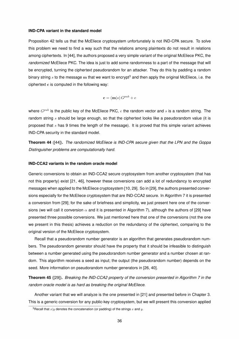
IND-CPA variant in the standard model
Proposition 42 tells us that the McEliece cryptosystem unfortunately is not IND-CPA secure. To solve
this problem we need to find a way such that the relations among plaintexts do not result in relations
among ciphertexts. In [44], the authors proposed a very simple variant of the original McEliece PKC, the
randomized McEliece PKC. The idea is just to add some randomness to a part of the message that will
be encrypted, turning the ciphertext pseudorandom for an attacker. They do this by padding a random
binary string s to the message m that we want to encrypt3 and then apply the original McEliece, i.e. the
ciphertext c is computed in the following way:
c = (m|s)Gpub + e
where Gpub is the public key of the McEliece PKC, e the random vector and s is a random string. The
random string s should be large enough, so that the ciphertext looks like a pseudorandom value (it is
proposed that s has 9 times the length of the message). It is proved that this simple variant achieves
IND-CPA security in the standard model.
Theorem 44 ([44]). The randomized McEliece is IND-CPA secure given that the LPN and the Goppa
Distinguisher problems are computationally hard.
IND-CCA2 variants in the random oracle model
Generic conversions to obtain an IND-CCA2 secure cryptosystem from another cryptosystem (that has
not this property) exist [21, 46], however these conversions can add a lot of redundancy to encrypted
messages when applied to the McEliece cryptosystem [10, 29]. So in [29], the authors presented conver-
sions especially for the McEliece cryptosystem that are IND-CCA2 secure. In Algorithm 7 it is presented
a conversion from [29]; for the sake of briefness and simplicity, we just present here one of the conver-
sions (we will call it conversion α and it is presented in Algorithm 7), although the authors of [29] have
presented three possible conversions. We just mentioned here that one of the conversions (not the one
we present in this thesis) achieves a reduction on the redundancy of the ciphertext, comparing to the
original version of the McEliece cryptosystem.
Recall that a pseudorandom number generator is an algorithm that generates pseudorandom num-
bers. The pseudorandom generator should have the property that it should be infeasible to distinguish
between a number generated using the pseudorandom number generator and a number chosen at ran-
dom. This algorithm receives a seed as input; the output (the pseudorandom number) depends on the
seed. More information on pseudorandom number generators in [26, 40].
Theorem 45 ([29]). Breaking the IND-CCA2 property of the conversion presented in Algorithm 7 in the
random oracle model is as hard as breaking the original McEliece.
Another variant that we will analyze is the one presented in [21] and presented before in Chapter 3.
This is a generic conversion for any public-key cryptosystem, but we will present this conversion applied3Recall that x|y denotes the concatenation (or padding) of the strings x and y.
36
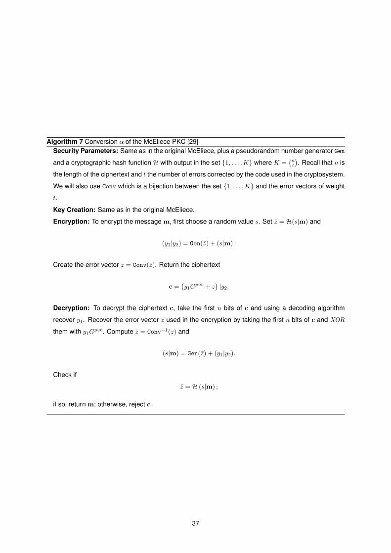
Algorithm 7 Conversion α of the McEliece PKC [29]Security Parameters: Same as in the original McEliece, plus a pseudorandom number generator Gen
and a cryptographic hash function H with output in the set 1, . . . ,K where K =(nt
). Recall that n is
the length of the ciphertext and t the number of errors corrected by the code used in the cryptosystem.
We will also use Conv which is a bijection between the set 1, . . . ,K and the error vectors of weight
t.
Key Creation: Same as in the original McEliece.
Encryption: To encrypt the message m, first choose a random value s. Set z = H(s|m) and
(y1|y2) = Gen(z) + (s|m) .
Create the error vector z = Conv(z). Return the ciphertext
c =(y1G
pub + z)|y2.
Decryption: To decrypt the ciphertext c, take the first n bits of c and using a decoding algorithm
recover y1. Recover the error vector z used in the encryption by taking the first n bits of c and XOR
them with y1Gpub. Compute z = Conv−1(z) and
(s|m) = Gen(z) + (y1|y2).
Check if
z = H (s|m) ;
if so, return m; otherwise, reject c.
37
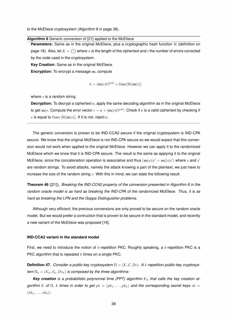
to the McEliece cryptosystem (Algorithm 8 in page 38).
Algorithm 8 Generic conversion of [21] applied to the McElieceParameters: Same as in the original McEliece, plus a cryptographic hash function H (definition on
page 18). Also, let K =(nt
)where n is the length of the ciphertext and t the number of errors corrected
by the code used in the cryptosystem.
Key Creation: Same as in the original McEliece.
Encryption: To encrypt a message m, compute
c = (m|s)Gpub + Conv[H(m|s)]
where s is a random string.
Decryption: To decrypt a ciphertext c, apply the same decoding algorithm as in the original McEliece
to get m|s. Compute the error vector e = c + (m|s)Gpub. Check if c is a valid ciphertext by checking if
e is equal to Conv [H(m|s)]. If it is not, reject c.
The generic conversion is proven to be IND-CCA2 secure if the original cryptosystem is IND-CPA
secure. We know that the original McEliece is not IND-CPA secure so we would expect that this conver-
sion would not work when applied to the original McEliece. However we can apply it to the randomized
McEliece which we know that it is IND-CPA secure. The result is the same as applying it to the original
McEliece, since the concatenation operation is associative and thus (m|s)|s′ = m|(s|s′) where s and s′
are random strings. To avoid attacks, namely the attack knowing a part of the plaintext, we just have to
increase the size of the random string s. With this in mind, we can state the following result.
Theorem 46 ([21]). Breaking the IND-CCA2 property of the conversion presented in Algorithm 8 in the
random oracle model is as hard as breaking the IND-CPA of the randomized McEliece. Thus, it is as
hard as breaking the LPN and the Goppa Distinguisher problems.
Although very efficient, the previous conversions are only proved to be secure on the random oracle
model. But we would prefer a contruction that is proven to be secure in the standard model, and recently
a new variant of the McEliece was proposed [16].
IND-CCA2 variant in the standard model
First, we need to introduce the notion of k-repetition PKC. Roughly speaking, a k-repetition PKC is a
PKC algorithm that is repeated k times on a single PKC.
Definition 47. Consider a public-key cryptosystem Π = (K, E , Dc). A k-repetition public-key cryptosys-
tem Πk = (Kk, Ek, Dck) is composed by the three algorithms:
Key creation is a probabilistic polynomial time (PPT) algorithm Kk that calls the key creation al-
gorithm K of Π, k times in order to get pk = (pk1, . . . , pkk) and the corresponding secret keys sk =
(sk1, . . . , skk);
38
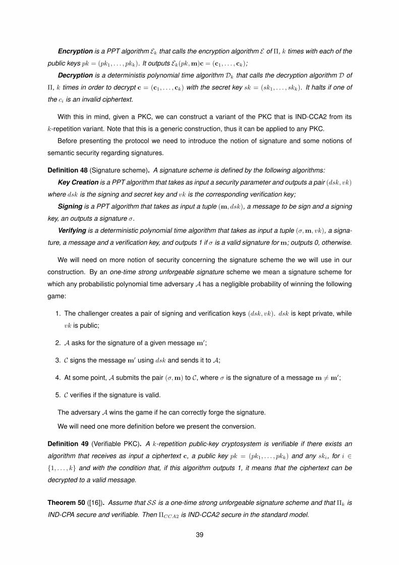
Encryption is a PPT algorithm Ek that calls the encryption algorithm E of Π, k times with each of the
public keys pk = (pk1, . . . , pkk). It outputs Ek(pk,m)c = (c1, . . . , ck);
Decryption is a deterministis polynomial time algorithm Dk that calls the decryption algorithm D of
Π, k times in order to decrypt c = (c1, . . . , ck) with the secret key sk = (sk1, . . . , skk). It halts if one of
the ci is an invalid ciphertext.
With this in mind, given a PKC, we can construct a variant of the PKC that is IND-CCA2 from its
k-repetition variant. Note that this is a generic construction, thus it can be applied to any PKC.
Before presenting the protocol we need to introduce the notion of signature and some notions of
semantic security regarding signatures.
Definition 48 (Signature scheme). A signature scheme is defined by the following algorithms:
Key Creation is a PPT algorithm that takes as input a security parameter and outputs a pair (dsk, vk)
where dsk is the signing and secret key and vk is the corresponding verification key;
Signing is a PPT algorithm that takes as input a tuple (m, dsk), a message to be sign and a signing
key, an outputs a signature σ.
Verifying is a deterministic polynomial time algorithm that takes as input a tuple (σ,m, vk), a signa-
ture, a message and a verification key, and outputs 1 if σ is a valid signature for m; outputs 0, otherwise.
We will need on more notion of security concerning the signature scheme the we will use in our
construction. By an one-time strong unforgeable signature scheme we mean a signature scheme for
which any probabilistic polynomial time adversary A has a negligible probability of winning the following
game:
1. The challenger creates a pair of signing and verification keys (dsk, vk). dsk is kept private, while
vk is public;
2. A asks for the signature of a given message m′;
3. C signs the message m′ using dsk and sends it to A;
4. At some point, A submits the pair (σ,m) to C, where σ is the signature of a message m 6= m′;
5. C verifies if the signature is valid.
The adversary A wins the game if he can correctly forge the signature.
We will need one more definition before we present the conversion.
Definition 49 (Verifiable PKC). A k-repetition public-key cryptosystem is verifiable if there exists an
algorithm that receives as input a ciphertext c, a public key pk = (pk1, . . . , pkk) and any ski, for i ∈
1, . . . , k and with the condition that, if this algorithm outputs 1, it means that the ciphertext can be
decrypted to a valid message.
Theorem 50 ([16]). Assume that SS is a one-time strong unforgeable signature scheme and that Πk is
IND-CPA secure and verifiable. Then ΠCCA2 is IND-CCA2 secure in the standard model.
39
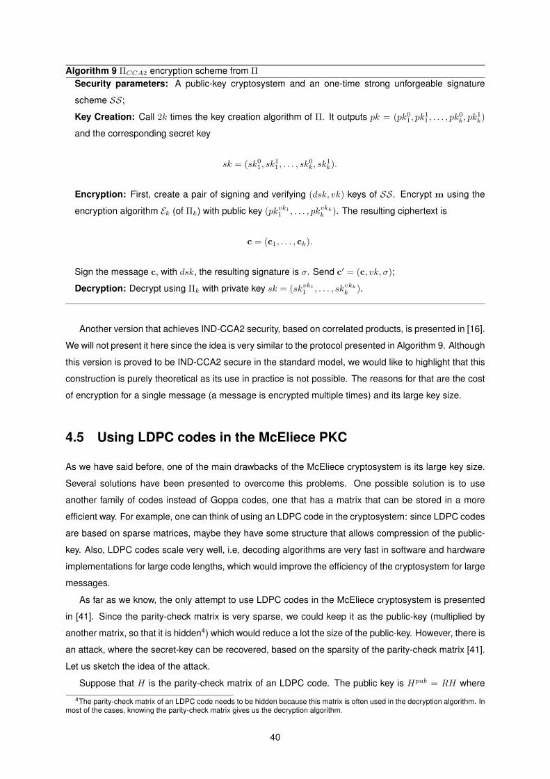
Algorithm 9 ΠCCA2 encryption scheme from Π
Security parameters: A public-key cryptosystem and an one-time strong unforgeable signature
scheme SS;
Key Creation: Call 2k times the key creation algorithm of Π. It outputs pk = (pk01, pk
11, . . . , pk
0k, pk
1k)
and the corresponding secret key
sk = (sk01, sk
11, . . . , sk
0k, sk
1k).
Encryption: First, create a pair of signing and verifying (dsk, vk) keys of SS. Encrypt m using the
encryption algorithm Ek (of Πk) with public key (pkvk11 , . . . , pkvkkk ). The resulting ciphertext is
c = (c1, . . . , ck).
Sign the message c, with dsk, the resulting signature is σ. Send c′ = (c, vk, σ);
Decryption: Decrypt using Πk with private key sk = (skvk11 , . . . , skvkkk ).
Another version that achieves IND-CCA2 security, based on correlated products, is presented in [16].
We will not present it here since the idea is very similar to the protocol presented in Algorithm 9. Although
this version is proved to be IND-CCA2 secure in the standard model, we would like to highlight that this
construction is purely theoretical as its use in practice is not possible. The reasons for that are the cost
of encryption for a single message (a message is encrypted multiple times) and its large key size.
4.5 Using LDPC codes in the McEliece PKC
As we have said before, one of the main drawbacks of the McEliece cryptosystem is its large key size.
Several solutions have been presented to overcome this problems. One possible solution is to use
another family of codes instead of Goppa codes, one that has a matrix that can be stored in a more
efficient way. For example, one can think of using an LDPC code in the cryptosystem: since LDPC codes
are based on sparse matrices, maybe they have some structure that allows compression of the public-
key. Also, LDPC codes scale very well, i.e, decoding algorithms are very fast in software and hardware
implementations for large code lengths, which would improve the efficiency of the cryptosystem for large
messages.
As far as we know, the only attempt to use LDPC codes in the McEliece cryptosystem is presented
in [41]. Since the parity-check matrix is very sparse, we could keep it as the public-key (multiplied by
another matrix, so that it is hidden4) which would reduce a lot the size of the public-key. However, there is
an attack, where the secret-key can be recovered, based on the sparsity of the parity-check matrix [41].
Let us sketch the idea of the attack.
Suppose that H is the parity-check matrix of an LDPC code. The public key is Hpub = RH where
4The parity-check matrix of an LDPC code needs to be hidden because this matrix is often used in the decryption algorithm. Inmost of the cases, knowing the parity-check matrix gives us the decryption algorithm.
40
R is a non-singular matrix. If R is sparse, then the public key RH is also sparse and this may allow
the compression of the key. To encrypt a message m, one just has to compute the generating matrix
G associated with Hpub and compute mSG + e where S is a non-singular public matrix that is used to
hide the message and e is a error vector of weight t. To decrypt, one just has to note that G and SG are
equivalent codes. So one can use H to decode the corrupt codeword and take out the error vector.
For the cryptosystem to be secure,Hpub should not admit the decoding using any decoding technique
for the LDPC codes and an adversary should not be able to retrieve H, or other H ′ equivalent to H and
that admits decoding, from Hpub. However, the sparsity of the public key matrix can be used to recover
some lines of the original parity-check matrix H which can be sufficient to allow the adversary to recover
the secret-key H [41].
We could avoid this attack if we choose R such that it is a dense matrix, and thus Hpub would be
dense. But then we could not reduce the public key size. So, the authors conclude that there is no
advantage in using a LDPC code over a Goppa code in the McEliece cryptosystem.
We believe that there is a big advantage on the usage of LDPC codes in cryptography. LDPC
codes are far more efficient than Goppa codes and we believe that this can be useful for hardware
implementations. We also believe that there are methods to prevent attacks like this one and take
advantage of the low complexity decoding algorithms of the LDPC codes in the McEliece cryptosystem.
That is what we are going to study in the next chapter.
41

42
Chapter 5
A New Cryptosystem: LDPC-based
McEliece
One of the most important features an asymmetric cryptosystem must fullfil is to be hardware imple-
mentable. Both RSA and elliptic curve cryptosystems (ECC) are highly demanding from the processing
time point of view, making them very slow to use, even in dedicated hardware implementations [38].
Moreover, both are not quantum resistant [51], motivating the community to look for post-quantum cryp-
tosystems [10]. One of the most promising candidates is the McEliece cryptosystem [39] that is based on
error-correcting codes, which are usually well behaved in hardware implementations. This cryptosystem
is the oldest one that is yet to be broken, by both classical and quantum algorithms.
Unfortunately, although much more efficient than RSA and ECC [18], the McEliece cryptosystem
has still some downsides: the key size is much larger than both RSA and ECC, which is a problem
for implementations (especially hardware implementations, where the memory available to store data
is very limited); and the decryption algorithm adquires a bottleneck effect as the key size grows since
the decoding algorithm of Goppa codes (the codes used in the original McEliece) takes to long as
the key size increases [38]. On the other hand, we know that LDPC codes [50] scale very well in
hardware implementations since their decoding algorithms are much simpler. But using LDPC codes in
the McEliece may not be as secure as using Goppa codes [41].
The McEliece cryptosystem has yet another downside: it is not indistinguishable against adaptive
chosen-ciphertext attacks (IND-CCA2). IND-CCA2 security is a crucial property for cryptosystems
nowadays as this notion reveals how much information an adversary can get on the message from
the ciphertext.
We propose a public-key encryption scheme that, given a message to encrypt, divides it into several
parts and encrypts each part individually using the McEliece cryptosystem with a Goppa code (such that
it can be implemented in parallel) and then encrypts the result using the McEliece cryptosystem with an
LDPC code. We can say that we add a little extra security to the traditional McEliece by encrypting
again using a LDPC-based McEliece cryptosystem. With this proposal, we aim to achieve the security
provided by traditional McEliece and the scalability provided by LDPC codes. Since our approach differs
43
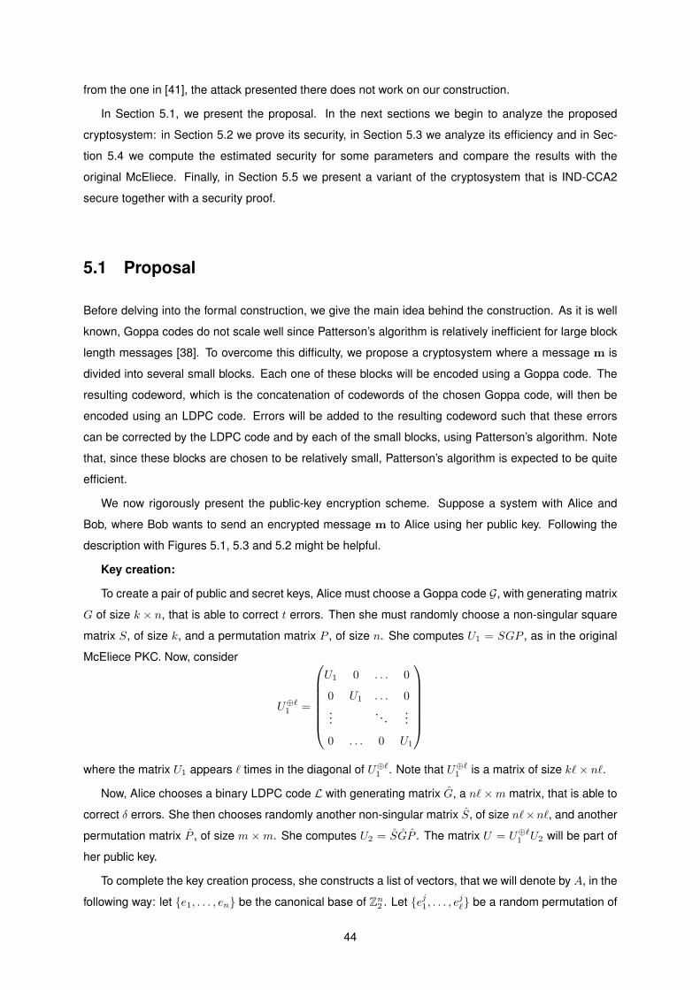
from the one in [41], the attack presented there does not work on our construction.
In Section 5.1, we present the proposal. In the next sections we begin to analyze the proposed
cryptosystem: in Section 5.2 we prove its security, in Section 5.3 we analyze its efficiency and in Sec-
tion 5.4 we compute the estimated security for some parameters and compare the results with the
original McEliece. Finally, in Section 5.5 we present a variant of the cryptosystem that is IND-CCA2
secure together with a security proof.
5.1 Proposal
Before delving into the formal construction, we give the main idea behind the construction. As it is well
known, Goppa codes do not scale well since Patterson’s algorithm is relatively inefficient for large block
length messages [38]. To overcome this difficulty, we propose a cryptosystem where a message m is
divided into several small blocks. Each one of these blocks will be encoded using a Goppa code. The
resulting codeword, which is the concatenation of codewords of the chosen Goppa code, will then be
encoded using an LDPC code. Errors will be added to the resulting codeword such that these errors
can be corrected by the LDPC code and by each of the small blocks, using Patterson’s algorithm. Note
that, since these blocks are chosen to be relatively small, Patterson’s algorithm is expected to be quite
efficient.
We now rigorously present the public-key encryption scheme. Suppose a system with Alice and
Bob, where Bob wants to send an encrypted message m to Alice using her public key. Following the
description with Figures 5.1, 5.3 and 5.2 might be helpful.
Key creation:
To create a pair of public and secret keys, Alice must choose a Goppa code G, with generating matrix
G of size k × n, that is able to correct t errors. Then she must randomly choose a non-singular square
matrix S, of size k, and a permutation matrix P , of size n. She computes U1 = SGP , as in the original
McEliece PKC. Now, consider
U⊕`1 =
U1 0 . . . 0
0 U1 . . . 0...
. . ....
0 . . . 0 U1
where the matrix U1 appears ` times in the diagonal of U⊕`1 . Note that U⊕`1 is a matrix of size k`× n`.
Now, Alice chooses a binary LDPC code L with generating matrix G, a n`×m matrix, that is able to
correct δ errors. She then chooses randomly another non-singular matrix S, of size n`×n`, and another
permutation matrix P , of size m ×m. She computes U2 = SGP . The matrix U = U⊕`1 U2 will be part of
her public key.
To complete the key creation process, she constructs a list of vectors, that we will denote by A, in the
following way: let e1, . . . , en be the canonical base of Zn2 . Let ej1, . . . , ej` be a random permutation of
44
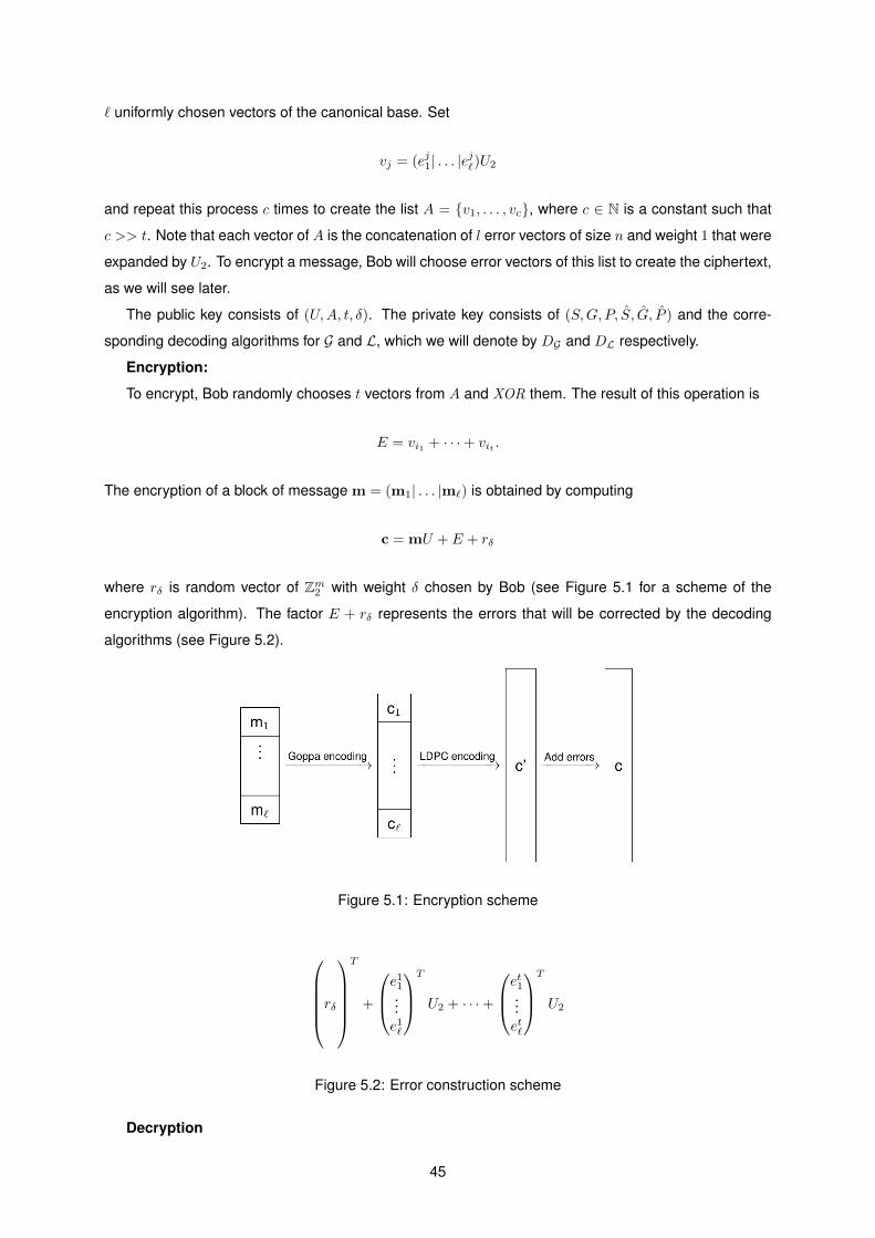
` uniformly chosen vectors of the canonical base. Set
vj = (ej1| . . . |ej`)U2
and repeat this process c times to create the list A = v1, . . . , vc, where c ∈ N is a constant such that
c >> t. Note that each vector of A is the concatenation of l error vectors of size n and weight 1 that were
expanded by U2. To encrypt a message, Bob will choose error vectors of this list to create the ciphertext,
as we will see later.
The public key consists of (U,A, t, δ). The private key consists of (S,G, P, S, G, P ) and the corre-
sponding decoding algorithms for G and L, which we will denote by DG and DL respectively.
Encryption:
To encrypt, Bob randomly chooses t vectors from A and XOR them. The result of this operation is
E = vi1 + · · ·+ vit .
The encryption of a block of message m = (m1| . . . |m`) is obtained by computing
c = mU + E + rδ
where rδ is random vector of Zm2 with weight δ chosen by Bob (see Figure 5.1 for a scheme of the
encryption algorithm). The factor E + rδ represents the errors that will be corrected by the decoding
algorithms (see Figure 5.2).
Figure 5.1: Encryption scheme
rδT
+
e11...e1`
T
U2 + · · ·+
et1...et`
T
U2
Figure 5.2: Error construction scheme
Decryption
45
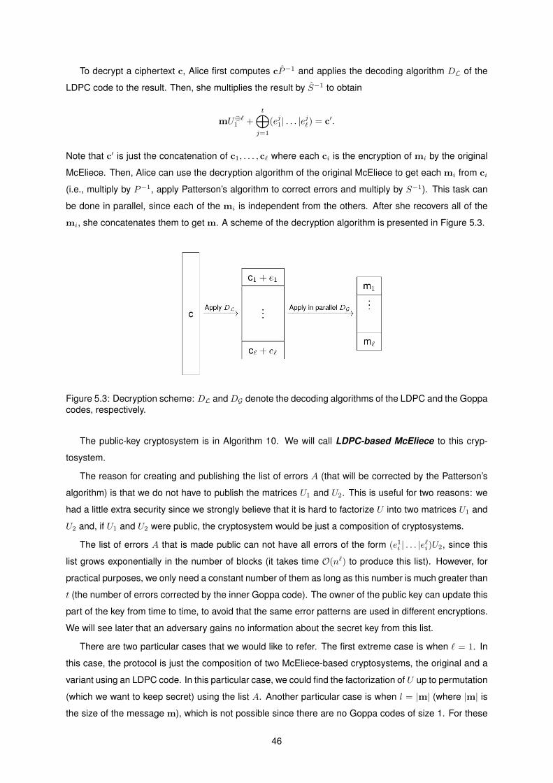
To decrypt a ciphertext c, Alice first computes cP−1 and applies the decoding algorithm DL of the
LDPC code to the result. Then, she multiplies the result by S−1 to obtain
mU⊕`1 +
t⊕j=1
(ej1| . . . |ej`) = c′.
Note that c′ is just the concatenation of c1, . . . , c` where each ci is the encryption of mi by the original
McEliece. Then, Alice can use the decryption algorithm of the original McEliece to get each mi from ci
(i.e., multiply by P−1, apply Patterson’s algorithm to correct errors and multiply by S−1). This task can
be done in parallel, since each of the mi is independent from the others. After she recovers all of the
mi, she concatenates them to get m. A scheme of the decryption algorithm is presented in Figure 5.3.
Figure 5.3: Decryption scheme: DL andDG denote the decoding algorithms of the LDPC and the Goppacodes, respectively.
The public-key cryptosystem is in Algorithm 10. We will call LDPC-based McEliece to this cryp-
tosystem.
The reason for creating and publishing the list of errors A (that will be corrected by the Patterson’s
algorithm) is that we do not have to publish the matrices U1 and U2. This is useful for two reasons: we
had a little extra security since we strongly believe that it is hard to factorize U into two matrices U1 and
U2 and, if U1 and U2 were public, the cryptosystem would be just a composition of cryptosystems.
The list of errors A that is made public can not have all errors of the form (e1i | . . . |e`i)U2, since this
list grows exponentially in the number of blocks (it takes time O(n`) to produce this list). However, for
practical purposes, we only need a constant number of them as long as this number is much greater than
t (the number of errors corrected by the inner Goppa code). The owner of the public key can update this
part of the key from time to time, to avoid that the same error patterns are used in different encryptions.
We will see later that an adversary gains no information about the secret key from this list.
There are two particular cases that we would like to refer. The first extreme case is when ` = 1. In
this case, the protocol is just the composition of two McEliece-based cryptosystems, the original and a
variant using an LDPC code. In this particular case, we could find the factorization of U up to permutation
(which we want to keep secret) using the list A. Another particular case is when l = |m| (where |m| is
the size of the message m), which is not possible since there are no Goppa codes of size 1. For these
46
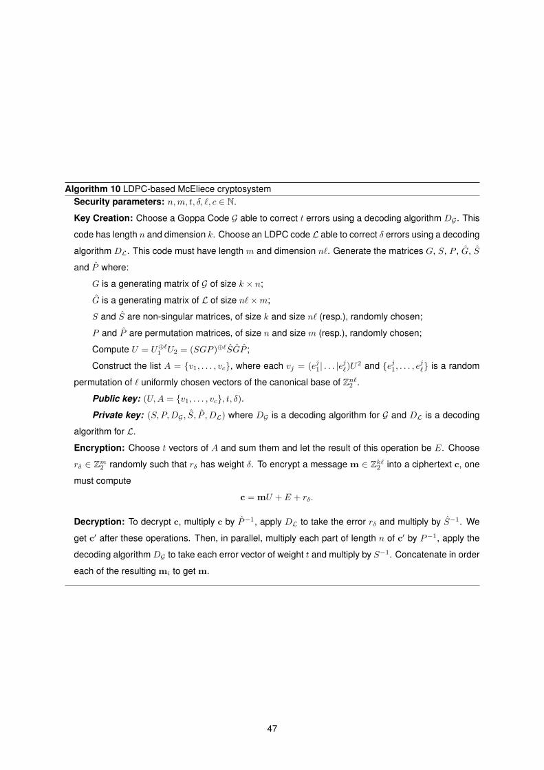
Algorithm 10 LDPC-based McEliece cryptosystemSecurity parameters: n,m, t, δ, `, c ∈ N.
Key Creation: Choose a Goppa Code G able to correct t errors using a decoding algorithm DG . This
code has length n and dimension k. Choose an LDPC code L able to correct δ errors using a decoding
algorithm DL. This code must have length m and dimension n`. Generate the matrices G, S, P , G, S
and P where:
G is a generating matrix of G of size k × n;
G is a generating matrix of L of size n`×m;
S and S are non-singular matrices, of size k and size n` (resp.), randomly chosen;
P and P are permutation matrices, of size n and size m (resp.), randomly chosen;
Compute U = U⊕`1 U2 = (SGP )⊕`SGP ;
Construct the list A = v1, . . . , vc, where each vj = (ej1| . . . |ej`)U
2 and ej1, . . . , ej` is a random
permutation of ` uniformly chosen vectors of the canonical base of Zn`2 .
Public key: (U,A = v1, . . . , vc, t, δ).
Private key: (S, P,DG , S, P ,DL) where DG is a decoding algorithm for G and DL is a decoding
algorithm for L.
Encryption: Choose t vectors of A and sum them and let the result of this operation be E. Choose
rδ ∈ Zm2 randomly such that rδ has weight δ. To encrypt a message m ∈ Zk`2 into a ciphertext c, one
must compute
c = mU + E + rδ.
Decryption: To decrypt c, multiply c by P−1, apply DL to take the error rδ and multiply by S−1. We
get c′ after these operations. Then, in parallel, multiply each part of length n of c′ by P−1, apply the
decoding algorithm DG to take each error vector of weight t and multiply by S−1. Concatenate in order
each of the resulting mi to get m.
47
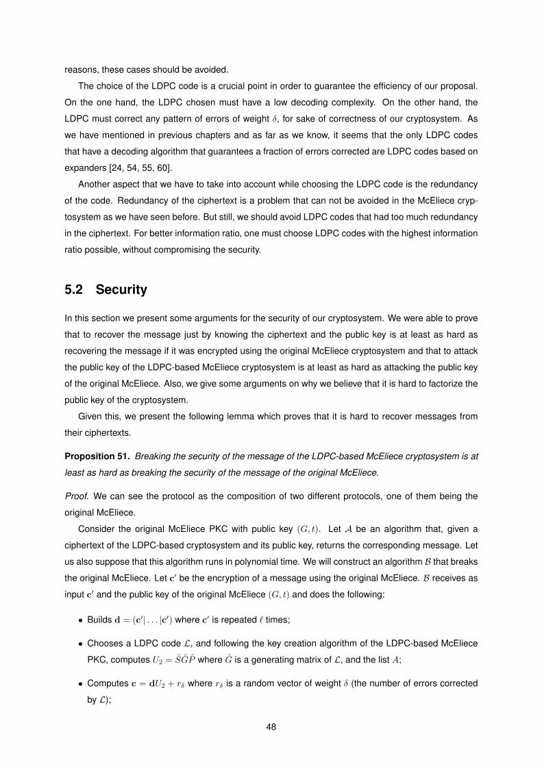
reasons, these cases should be avoided.
The choice of the LDPC code is a crucial point in order to guarantee the efficiency of our proposal.
On the one hand, the LDPC chosen must have a low decoding complexity. On the other hand, the
LDPC must correct any pattern of errors of weight δ, for sake of correctness of our cryptosystem. As
we have mentioned in previous chapters and as far as we know, it seems that the only LDPC codes
that have a decoding algorithm that guarantees a fraction of errors corrected are LDPC codes based on
expanders [24, 54, 55, 60].
Another aspect that we have to take into account while choosing the LDPC code is the redundancy
of the code. Redundancy of the ciphertext is a problem that can not be avoided in the McEliece cryp-
tosystem as we have seen before. But still, we should avoid LDPC codes that had too much redundancy
in the ciphertext. For better information ratio, one must choose LDPC codes with the highest information
ratio possible, without compromising the security.
5.2 Security
In this section we present some arguments for the security of our cryptosystem. We were able to prove
that to recover the message just by knowing the ciphertext and the public key is at least as hard as
recovering the message if it was encrypted using the original McEliece cryptosystem and that to attack
the public key of the LDPC-based McEliece cryptosystem is at least as hard as attacking the public key
of the original McEliece. Also, we give some arguments on why we believe that it is hard to factorize the
public key of the cryptosystem.
Given this, we present the following lemma which proves that it is hard to recover messages from
their ciphertexts.
Proposition 51. Breaking the security of the message of the LDPC-based McEliece cryptosystem is at
least as hard as breaking the security of the message of the original McEliece.
Proof. We can see the protocol as the composition of two different protocols, one of them being the
original McEliece.
Consider the original McEliece PKC with public key (G, t). Let A be an algorithm that, given a
ciphertext of the LDPC-based cryptosystem and its public key, returns the corresponding message. Let
us also suppose that this algorithm runs in polynomial time. We will construct an algorithm B that breaks
the original McEliece. Let c′ be the encryption of a message using the original McEliece. B receives as
input c′ and the public key of the original McEliece (G, t) and does the following:
• Builds d = (c′| . . . |c′) where c′ is repeated ` times;
• Chooses a LDPC code L, and following the key creation algorithm of the LDPC-based McEliece
PKC, computes U2 = SGP where G is a generating matrix of L, and the list A;
• Computes c = dU2 + rδ where rδ is a random vector of weight δ (the number of errors corrected
by L);
48
• Applies A with inputs c and the public key (U = G⊕`U2, A, t, δ); A will output m = (m′| . . . |m′)
where m′ is repeated ` times;
• Output m′.
Each of these tasks can be done in polynomial time, given that A runs in polynomial time. Thus, B
runs in polynomial time and therefore we can break McEliece in polynomial time.
We have proved that in our cryptosystem it is hard to recover the message from the ciphertext. So
now we will talk about the security of the public key.
Proposition 52. Breaking the security of the public key of the LDPC-based McEliece cryptosystem is
at least as hard as breaking the security of the public key of the original McEliece.
Proof. The reduction is similar to the previous one: consider the original McEliece PKC with public key
(G, t). Let A be an algorithm that, given a public key of the LDPC-based cryptosystem, returns the
corresponding secret key. Let us also suppose that this algorithm runs in polynomial time. We will
construct an algorithm B that breaks the public key of the original McEliece. B receives as input (G, t)
and does the following:
• Builds U⊕`1 = G⊕`;
• Chooses a LDPC code L that corrects δ, and, following the key creation algorithm of the LDPC-
based McEliece PKC, computes U2 = SGP where G is a generating matrix of L. Also, creates the
list A;
• Computes U = U⊕`1 U2;
• Applies A with inputs (U,A, t, δ); A will output (S, P,DG , S, P ,DL) where S and P are part of the
factorization of G (according to the McEliece protocol) and DG and DL are the decoding algorithms
for the Goppa code and for the LDPC code respectively used;
• Output (S, P,DG) which is the secret key of the McEliece cryptosystem with public key G.
Each of these tasks can be done in polynomial time, given that A runs in polynomial time. Thus, B
runs in polynomial time and therefore we can break the public key of the McEliece in polynomial time.
Although recovering the secret key is hard (given that breaking the McEliece cryptosystem is hard),
it may be a problem if an adversary is able to factor the public key U . Recall that the public key is
(U,A = v1, . . . , vc, t, δ) where U is a matrix with k` lines and m columns and it is the product of U⊕`1
(a k`× n` matrix) by U2 ( n`×m matrix). Since U⊕`1 represents the concatenation of ` original McEliece
cryptosystem (which is conjectured to be indistinguishable from a uniformly chosen matrix), the real
menace to the cryptosystem is if an adversary could find the which LDPC is being used. If it could
do that, then breaking the cryptosystem would be equivalent to break the original McEliece for small
parameters.
49
To find the LDPC code used in the cryptosystem, an adversary would need to factor the matrix U .
Note that some information is leaked from the list A, namely the parameters of the LDPC code used. To
find the parameters, an adversary can proceed in the following way: The adversary chooses a vector
from the list A. Then it chooses another vector from A that is linearly independent from the first chosen
vector. Again, it chooses another vector that is linearly independent from the first two chosen vectors. It
does this until there is no linearly independent vector to choose. Most likely, it will get a set of n` vectors
linearly independent since each vector
vj = ujU
where uj = (ej1| . . . |ej`) is a vector of size n`. Let v′1, . . . , v′n` be the list obtained from this procedure.
The matrix
U ′2 =
v′1...
v′n`
is a change of basis of the matrix U2. With this, the adversary can get the value n` and, thus, it gets the
parameters of the LDPC code, which is a n` dimensional code of length m. But note that it has no more
information, particularly on the new basis, since it does not know which basis u′1, . . . , u′n` was used to
construct the list of vectors v′1, . . . , v′n`. So, it can not recover U2 from its matrix U ′2.
Another threat to our cryptosystem is the attack presented in [41] and in the previous chapter. But
note that this attack only works if the parity-check matrix of the LDPC code is made public (more pre-
cisely, the parity-check times another sparse matrix is made public) , which is not the case in our ap-
proach.
With this in mind, we conclude that every known attack on the cryptosystem does not seem to work.
Even if an adversary was able to somehow find the matrix U2 or the corresponding parity-check matrix,
it would still have to find the number of blocks ` and to break ` McEliece ciphertexts. This lead us to
strongly believe that it is hard to recover the secret key from the public key. Given this, we believe that
our cryptosystem is secure.
Note that the cryptosystem is also robust against quantum attacks, otherwise we could quantumly
attack the original McEliece as well. Also, since our protocol is based in the McEliece, we strongly
believe that every attack on the McEliece (and every way to defend it from attacks) can be adapt to our
cryptosystem.
If instead of using an LDPC code, we use a Goppa code (with larger parameters) we can prove that
it is hard to factor the public key. To prove that, we assume that the Goppa Distinguisher problem is hard
and, therefore, we cannot distinguish the public key from a uniformly chosen matrix. But using a Goppa
code may compromise the efficiency of the cryptosystem.
50
5.3 Efficiency
The efficiency of the LDPC-based McEliece cryptosystem depends greatly on the choice of the LDPC
used. In this section, we will analyze the efficiency of the proposed cryptosystem in terms of time
complexity and circuit complexity. For the former, a unit of time is a binary operation; we will measure
the time of an algorithm as the number of binary operations it takes. For the circuit complexity analysis,
we will analyze what is the size and depth of a circuit, using AND, OR and NOT gates, that computes
the algorithm.
Time complexity
In the following, we will use the same notation as in the previous section. Consider a cryptosystem using
a k- dimensional Goppa code of length n defined by (g, L), where g is a polynomial with coefficients
in F2p , that can correct t errors, and using a (n`)-dimensional LDPC code of length m that can correct δ
errors.
First, we need an auxiliary lemma which tells us the time complexity of multiplying two matrices.
Lemma 53. Let Mn×m and M ′m×p be two matrices. The complexity of multiplying these two matrices is
O(nmp).
The proof of this lemma is done by evaluating the complexity of schoolbook matrix multiplication
between these two matrices. This lemma is obviously necessary for the analysis of our algorithm since
it uses a lot of matrix operations.
Proposition 54. The time complexity of the encryption algorithm of our cryptosystem is
O(mk`+ T trand + T δrand
)where T trand and T δrand are the times that takes to choose t vectors from A and to create an error vector
of weight δ, respectively.
Proof. The computational complexity of the encryption is just the complexity of multiplying a vector by
a matrix plus the time of choosing t vectors from the list A, summing them and the time of choosing a
random vector of weight δ.
Using the lemma above, we conclude that the time complexity of computing the ciphertext of a given
message is
O(mk`) +O(T trand) +O(T δrand)
where T trand is the time needed to choose t vectors from the list A and some them, and T δrand is the time
needed to create an error vector of size m and weight δ. The factor mk` corresponds to the multiplication
of the message m (of size k`) by the public key U (of size k`×m).
Proposition 55. The time complexity of the decryption algorithm of our cryptosystem is
O(`ntp2 + TDLDPC + km2 + kn2`2
)51
where TDLDPC is the time it takes to decode a corrupt word using the LDPC code.
Proof. Here, the analysis is a bit more complex. We will assume that the owner of the secret key
has previously computed and stored the inverse of the matrices P , S, P and S. So the time that the
decryption algorithm takes is the time of multiply matrices plus the time of decoding a Goppa code `
times and the time of decoding an LDPC code.
As before, let us assume that the Goppa code used in the cryptosystem is a k-dimensional code
of length n with generator polynomial g defined in F2p and that the LDPC used is a (n`)-dimensional
code of length m. The decryption algorithm of the original McEliece cryptosystem, as we have seen in
Chapter 4 (Theorem 41), takes O(ntp2) binary operations. Note that the Patterson’s algorithm will be
applied ` times. So, the complexity of the decryption algorithm is
O(`ntp2
)+O
(TDLDPC + km2 + kn2`2
)where the factor km2 corresponds to the multiplication by the matrix P , the factor kn2`2 corresponds to
the multiplication by the matrix S (by Lemma 53) and TDLDPC is the time it takes to decode a word using
the LDPC code.
Proposition 56. The time complexity of the key creation algorithm of our cryptosystem is
O(k2n+ n2 + t3(n− k) + (n− k)3 + T CLDPC + km2 + kn2`2 + ck`m
)where T CLDPC is the time it takes to create an LDPC code.
Proof. Note that, to create a pair of keys for the LDPC-based McEliece cryptosystem, we create a pair
of keys for the original McEliece cryptosystem plus an LDPC code, matrices P and S and multiply them.
This takes
O(TKMcEliece
)+O
(T CLDPC + km2 + kn2`2
)where TKMcEliece is the time it takes to create a pair of keys for the original McEliece, T CLDPC is the time
it takes to create a generating matrix of an LDPC code and the factors km2 and kn2`2 correspond to the
multiplication by the matrices P and S respectively. The time it takes to create the matrix U⊕`1 is O(`nk),
which is negligible for the complexity. We also need to create a list A of errors, which can be done in
O(ck`m) operations. Hence, the time complexity is
O(k2n+ n2 + t3(n− k) + (n− k)3 + T CLDPC + km2 + kn2`2 + ck`m
).
Recall that the list A can be renewed from time to time. The renovation of the list of errors A can be
done with O(ck`m) operations.
The key creation algorithm is not as fast as the algorithms of encryption and decryption, but we would
like to stress that the key creation is called only once (hopefully) while the others are called several times.
52
The main idea to retain is that LDPC codes usually have low time complexity decoding algorithms
comparing to Goppa codes. This means that LDPC codes typically scale much better than Goppa
codes [37]. Thus, the encryption and decryption for a largem should be faster than the original McEliece,
using a code with the same length.
Another aspect we would like to highlight is the fact that this cryptosystem is extremely parallelizable.
All the Goppa blocks can be implemented in parallel making the decryption algorithm much faster than
if it was implemented sequentially. Also, the cryptosystem uses a lot of matrix multiplication in its en-
cryption and decryption algorithms, and this operation that can also be parallelized. This fact makes the
LDPC-based McEliece cryptosystem very useful for hardware implementations. To support this fact, we
will analyze the circuit complexity of the cryptosystem.
Circuit complexity
Before we start, let us check some basic notions on circuit complexity. While computational complexity
analyzes the space and time resources needed for a program to run, circuit complexity studies the size
(the number of gates) of the circuit that computes a program using only AND, OR and NOT gates.
Also, we evaluate these circuits in terms of depth, which can express the parallelization capacity of a
program. Note that there is a different circuit for inputs of different size, so we analyze the size of the
circuit in terms of the size of the input.
The following result gives us an upper-bound for the circuit-size complexity of a program from its time
complexity.
Lemma 57 ([53]). Let T (n) : N → N. If A is a program that runs in time O (T (n)) then A can be
implemented in a circuit of size O(T (n)2
)where n is the size of the input.
The proof of this theorem is done by implementing each instruction of A sequentially in a circuit. So,
the theorem tells us that A can be implemented in a circuit of size (and depth) O(T (n)2
)but does not
guarantee that there is not a circuit that computes A with a smaller size and depth, i.e., it only gives us
an upper-bound for the circuit size (and does not give a clue about the lower-bound). A smaller circuit
may possibly be constructed by optimizing the number of gates or parallelizing some instructions of A
for smaller depth complexity.
Before we start the analysis, recall that our cryptosytem uses many matrix operations, so we prove
the following lemma that gives us an upper-bound for the circuit complexity of multiplying two matrices.
Lemma 58. Let C be a circuit that computes the product of two matrices An×k and Bk×m. Then C has
size O(nkm) and depth O(log k).
Proof. The input size is the size of A plus the size of B, thus the total size is nk+mk. Let Cn×m = AB.
The entries of C can be computed in the following way
cij =
k∨l=1
(ail ∧ blj).
53
So we need an AND gate to compute each term ail ∧ blj which gives us a total of nmk AND gates.
Then, we need k − 1 OR gates for each of the∨l(ail ∧ blj) for fixed i and j. We can compute that using
a binary tree, computing two by two and this gives us a circuit of depth log k.
The circuit has size O(nmk + (k − 1)) = O(nmk) and depth O(log k).
Let us start by analyzing the circuit complexity of the encryption algorithm.
Proposition 59. The encryption algorithm of the LDPC-based McEliece cryptosystem can be imple-
mented with a circuit of size O(mk`) and depth O(log k`) plus the circuit size and depth of choosing t
random vectors of A and a random vector of size m and weight δ.
Proof. For the encryption, we need to compute the circuit complexity of multiplying a matrix Uk`×m by a
message vector m of size k`,
c1×m = m1×k`Uk`×m.
Here, the size of the input is mk`+ k`.
Using the Lemma 58, the circuit complexity of the encryption is O(mk`) plus the size of the circuit
to choose the random vectors. The circuit-depth complexity is O(log k`) plus the circuit-depth to choose
the random vectors.
The next theorem gives us the circuit complexity of decrypting a ciphertext using the decryption
algorithm presented for our cryptosystem.
Proposition 60. The decryption algorithm of the LDPC-based McEliece cryptosystem can be imple-
mented with a circuit of size
O(m2 + (n`)2 + (ntp2)2 + k2 + SDLDPC
)and depth
O(log(mn2`k) + (ntp2)2 +DSDLDPC
)where SDLDPC is the circuit size of the decoding algorithm of the chosen LDPC and DSDLDPC its depth.
Proof. Once again, we assume that we have previously computed and stored the inverse of the matrices
in the secret key. These are the tasks to perform in the decryption process:
• matrix multiplication P−1 which can be implemented with a circuit of sizeO(m2) and depthO(logm)
by Lemma 58;
• decode a corrupted codeword of the LDPC code, which depends on the choice of the LDPC code.
Let SDLDPC be the circuit size of the decoding algorithm of the chosen LDPC and DSDLDPC its
depth;
• matrix multiplication S−1 which can be implemented in a circuit of sizeO(n2`2) and depthO(log n`);
• matrix multiplication P−1, repeated ` times, which can be done in parallel with a circuit of size
O(n2) and depth O(log n);
54
• decode a corrupted codeword of the Goppa code. By Lemma 57, this task can be implemented
with a circuit of size (and depth) O((ntp2)2
);
• matrix multiplication S−1, repeated ` times, which can be done in parallel with a circuit of size
O(k2) and depth O(log k)
This gives an upper-bound for the size of the circuit of
O(m2 + n2`2 + n2 + (ntp2)2 + k2
)= O
(m2 + (n`)2 + (ntp2)2 + k2
)and depth of
O(logm+ log n`+ log n+ (ntp2)2 + log k
)= O
(log(mn2`k) + (ntp2)2
).
Note that, as long as we choose the length of the Goppa code to be small (parameter n and, con-
sequently, both parameters t and p), the cryptosystem has a very low depth complexity and therefore
should be quite efficient.
5.4 Parameters
We will analyze the parameters to use and the security expected of the cryptosystem taking into account
the classical and the quantum information set decoding attacks (see Chapter 4). Recall that, for a k
dimensional code of size n that corrects t errors, the complexity of the classical information set decoding
attack is
Ω
(n2
(nk
)(n−tk
))
and the complexity of the quantum information set decoding attack is
Ω
(n2
√ (nk
)0.29
(n−tk
)) .If one wants to use the classical information set decoding to our cryptosystem, note that one needs
to use it to decode the LDPC code and then to decode each of the Goppa blocks. So, the complexity
of this attack to our cryptosystem is Ω(m2(mn`
)/(m−δn`
)), which corresponds to decode the LDPC code,
plus Ω(`n2(nk
)/(n−tk
)), which corresponds to decode each of the Goppa blocks. A lower-bound in the
total complexity of the attack is
Ω
(m2
(mn`
)(m−δn`
) + `n2
(nk
)(n−tk
)) .For a choice of parameters m = 1024, n = 64, ` = 12, k = 30, δ = 70, t = 4 the expected number
of operations of an information set decoding attack is roughly 2172. For these parameters, the key size
(in the systematic form) is (m − k`) × k` ≈ 30KB (kilobyte), which is much smaller than the McEliece
55
public key. For the same level of security, the key size of our cryptosystem is roughly ten times smaller
than the McEliece key size.
Analogously, the complexity of the quantum set decoding attack for our cryptosystem is
Ω
(m2
√ (mn`
)0.29
(m−δn`
) + `n2
√ (nk
)0.29
(n−tk
)) .For the same choice of parameters above, the cryptosystem has a quantum security of approximately
297 operations.
With this in mind, we can estimate parameters for our cryptosystem. Those estimates are presented
in Table 5.1.
Parameters Public-key size(systematic) Security PQ Security
m n ` k δ t1024 64 12 30 70 4 30 KB ≈ 2172 ≈ 297
1000 12 50 4 60 2 20 KB ≈ 2103 ≈ 263
Table 5.1: Parameters for the LDPC-based McEliece cryptosystem
To maximize the security we need to enlarge the size of the Goppa blocks. This leads to an increase
in the number of operations for the information set decoding attack. But, as we have seen in the previous
section, if each of the Goppa blocks become too large, the cryptosystem is not so efficient. So, there
is a trade off between security and efficiency: if one needs efficiency then it is better to choose smaller
Goppa blocks; if one is looking for maximizing the security, one needs to choose larger Goppa blocks.
5.5 On the indistinguishability of the LDPC-based McEliece
Unfortunately, the LDPC-based McEliece is not IND-CCA2 secure, since it is extremely malleable (like
the original McEliece).
Proposition 61. The LDPC-based McEliece is not IND-CCA2 secure.
Proof. To prove that the LDPC-based McEliece is not IND-CCA2 secure, we will build an adversary A
that has a non-negligible probability of winning the IND-CCA2 game presented in page 20.
A follows this strategy: when A receives the challenge-ciphertext c = mbU + E + rδ, she chooses
a message m, different from m0 and m1, and computes c′ = mU + c. Note that c′ is a valid ciphertext.
So, A can ask the decryption oracle for the decryption of c′, which is m + mb. Now, since A knows m,
m0 and m1, she can discover exactly what is the value of b. We conclude that the advantage of A in the
IND-CCA2 game for the LDPC-based McEliece is maximal.
In this section we will propose an IND-CCA2 variant of the LDPC-based McEliece cryptosystem. As
we have highlighted before in this thesis, IND-CCA2 property is a crucial security property for cryptosys-
tems nowadays (see Chapter 3).
56
For our IND-CCA2 variant of the cryptosystem we will need the concept of cryptographic hash func-
tion, previously introduced in Chapter 3. Recall that a cryptographic hash function takes an input of any
size and maps it to a fixed size output such that it is difficult to invert and to find collisions.
To achieve the IND-CCA2 property, we will take out the malleability of the cryptosystem. The idea is
very simple: the error that will be corrected by the LDPC (denoted by rδ, just like in previous sections)
that will be used in the construction of a ciphertext will be chosen accordingly to a cryptographic hash
function. Given a ciphertext, if we do that, it becomes infeasible to create other valid ciphertexts from a
valid one, which is the idea of the IND-CCA2 attack presented in the proof above.
We choose a cryptographic hash function H such that H maps inputs of arbitrary size to a fixed size
output. Let K =(mδ
), where δ is the number of errors corrected by the LDPC code of length m in the
cryptosystem1 and let us choose H such that its output set is 1, . . . ,K. We define a new function He
using H:
He(x) := Conv [H(x)]
where Conv is a bijection between 1, . . . ,K and the error vectors of size m and weight δ. Note that, as
m grows, K grows as well. So the probability of finding collisions for this function is exponentially low.
We now formally present the construction. When we encrypt a message m, first we choose a random
value s of fixed size and compute
r = He(m|s).
Also, instead of just encrypting m, we will encrypt m|s. This will be the error vector to be added to the
ciphertext in the encryption algorithm and that will be corrected by the LDPC decoding algorithm. In the
decryption, one just has to verify if rδ = He(m|s). If so, the ciphertext was a valid one. If not, then the
ciphertext is rejected as invalid.
Algorithm 11 briefly describes the IND-CCA2 version of the LDPC-based McEliece.
Algorithm 11 IND-CCA2 version of LDPC-based McElieceSecurity parameters: Same as in LDPC-based McEliece cryptosystem plus a cryptographic hash
functions H.
Key Creation: Same as in LDPC-based McEliece.
Encryption: Choose a random string s and encrypt m|s using the encryption algorithm of the LDPC-
based McEliece, except that the random vector of weight δ will not be chosen randomly, but accord-
ingly to H, i.e., rδ = He(m|s). The ciphertext will be
c = (m|s)U + E +He(m|s).
Decryption: Apply the decryption algorithm of the LDPC-based McEliece to get m|s. Compute the
error vector rδ = c+ (m|s)U +E. Check if c is a valid ciphertext by checking if rδ is equal to He(m|s).
If it is not, reject c.
1Once again, we see the importance of choosing an LDPC that corrects a constant fraction of errors.
57
This protocol is similar to the Fujisako-Okamoto generic conversion, presented in Chapter 3. The
difference is that, in our conversion, only part of the randomization of the cryptosystem is determined
by the cryptographic hash function while, in the generic conversion of Fujisako and Okamoto, all the
randomization is determined by the cryptographic hash function.
We will now prove that this algorithm is indeed IND-CCA2 secure. First, we show that it is IND-CPA
secure.
Theorem 62. The LDPC-based McEliece cryptosystem is IND-CPA secure in the random oracle model
given that the randomized McEliece is IND-CPA secure. Thus, it is IND-CPA secure given that the LNP
and the Goppa Distinguisher problems are hard.
Proof. Consider the following two games:
Game 1: IND-CPA game where m is encrypted in the following way: (m|s)U + E + r, where r is a
random vector of weight δ.
Game 2: IND-CPA game where m is encrypted in the following way: (m|s)U + E +He(m|s).
We will prove the theorem by proving a couple of claims.
Claim 1: From the adversary’s point of view, Game 1 and Game 2 are computationally indistinguish-
able given that H is a cryptographic hash function.
Since the adversary does not know the random value s chosen in the encryption and H is a cryp-
tographic hash function, the value He(m|s) will look completely random for the adversary which means
that it can not distinguish between He(m|s) and a random vector of weight δ. So, it can not distinguish
between these two games.
Claim 2: The advantage of an adversary A in Game 1 is negligible.
The proof is by reduction. Suppose that the advantage of an adversary A is non-negligible for Game
1, i.e.,
AdvAGame 1(γ) > ε
where γ is the security parameters and ε is a non-negligible value. Then we will construct an adversary
B that has non-negligible advantage of breaking the IND-CPA security of the randomized McEliece
cryptosystem (which is a hard problem, given that both LPN and Goppa Distinguisher problems are
hard, as we have seen in the previous chapter).
B works as follows:
1. B receives a public key of the randomized McEliece cryptosystem U1 from the challenger. B
chooses an LDPC capable of correcting δ errors, with generating matrix U2 (which it will keep it to
itself) and computes U = U1.U2. B simulates A and gives it U as a public key for the cryptosystem;
2. Eventually, A outputs two messages m0,m1. B outputs these two messages to the challenger;
3. B receives c from the challenger, where c is a randomized McEliece ciphertext of mb, with b ∈
0, 1;
4. B computes c′ = cU2+r, where r is a random vector of weight δ. It submits c′ toA as the challenge
ciphertext;
58
5. B outputs whatever A outputs.
The advantage of B of breaking the IND-CPA security of the randomized McEliece is
AdvRM,Bind−cpa(γ′) = AdvAGame 1(γ) > ε
where γ′ is the security parameter of the randomized McEliece. Since this advantage is proved to be
negligible, we conclude that the advantage of breaking the IND-CPA security of the IND-CCA2 version
of the LDPC-based McEliece cryptosystem is also negligible.
Theorem 63. For any qH , there exists a (λ)-extractor K for the IND-CCA2 version of the LDPC-based
McEliece, where 1− λ is a negligible value.
Proof. Let (U,A, t, δ) be the public key of the LDPC-based McEliece. We will denote the range of U by
Im(U). The specification of K is presented in Algorithm 12. Let τ = (h1,H1), . . . , (hqH ,HqH ) be a list
of questions to the random oracle from an adversary and respective answers, η = y1, . . . , yqE be a list
of answers to queries to the encryption oracle by the same adversary and let c /∈ η be a ciphertext.
Algorithm 12 Specification of knowledge extractor Kinput: (τ, η, c, U);
output: m.
for qH times do
c′ = c−Hi where (hi,Hi) ∈ τ ;
if c′ ∈ Im(U) then
m = (hi)k` (the first k` bits of hi);
break;
else
m =⊥, where ⊥ is the empty string;
end if
end for
return m.
Checking if the vector c′ is in the range of the linear transformation U can be done in polynomial time
(for example, by checking if the equation c′ = Ux has solution or not).
K runs in time
t′ = qH
(|c|+ TIm(U) + k`
)where |c| is the length of c and TIm(U) is the time it takes to evaluate if c′ is in the image of U . So the
time complexity is
O(qH(|c|+ TIm(U) + k`)
).
Now, let us analyze the success probability of K. Let D be the decryption algorithm of the IND-CCA2
version of the LDPC-based McEliece, sk its secret key and let ζ be an upper-bound for the probability of
59
finding a collision for the hash function H, i.e.,
Pr[find x, y : H(x) = H(y)
]≤ ζ.
Let us define two events: Fail and AskH. Fail happens when m 6= D(c, sk). AskH happens when
there exists (hi,Hi) ∈ τ such that c′ = c−Hi is in the image of U . Then, we have
Pr(Fail) = Pr(Fail|AskH).P r(AskH) + Pr(Fail|¬AskH).P r(¬AskH)
≤ Pr(Fail|AskH) + Pr(Fail|¬AskH)
≤ ζ +1(mδ
) .If AskH is true, then the probability of K failing is equal to the probability of finding a collision for the
hash function H. So
Pr(Fail|AskH) ≤ ζ.
When AskH is false, then K will output m =⊥, i.e., K will consider c an invalid ciphertext. If c is a valid
ciphertext, that means that the adversary B managed to create a valid ciphertext without querying the
oracle H. So,
Pr(Fail|¬AskH) =1(mδ
)which is the probability of guessing the right error vector for a given message m and a random value s.
Hence, the probability of K not failing is
Pr(¬Fail) = 1− Pr(Fail)
≥ 1−(ζ +
1(mδ
))
and we conclude that K is a λ- knowledge extractor, where
λ ≥ 1−(ζ +
1(mδ
)).Since ζ + 1
(mδ )is a negligible value, we have that λ ≈ 1.
We are now able to state that this version of the cryptosystem has the IND-CCA2 property, by plug-
ging the two previous theorems and noting that PA-security implies IND-CCA2 security (see Chapter 3,
Theorem 29).
Theorem 64. The IND-CCA2 version of the LDPC-based McEliece is IND-CCA2 secure given that the
randomized LDPC-based McEliece is IND-CPA secure.
As a corollary, we have that this version is also non-malleable.
Corollary 65. The IND-CCA2 version of the LDPC-Based McEliece cryptosystem is NM-CCA2 secure.
60
Chapter 6
Conclusions
Post-quantum will soon be a reality in our everyday lives. So, it is essential to find new efficient and
secure post-quantum protocols and that is what the cryptographic community is doing at the moment.
Currently, the McEliece cryptosystem is a serious candidate to become one of the most used cryp-
tosystems in practice very soon. It has a simple and elegant structure and, although there is no formal
security proof, nobody has a single clue on how to break it, either classically or quantumly. However the
cryptosystem has still some downsides being the key size the most problematic.
We were able to construct a variant of the McEliece cryptosystem which we called the LDPC-based
McEliece cryptosystem. This cryptosystem uses LDPC codes which have very efficient decoding algo-
rithms and turn the decryption even faster and simpler to implement. Also, the composition of Goppa
codes and LDPC codes used in the new construction dramatically decreases the key size comparing to
the original McEliece. We believe that these two upgrades turn our cryptosystem suitable for software
and hardware applications.
We were able to prove both the security of the ciphertext and the security of the public-key for this
new construction. We were not able to prove that it is hard to factorize the public-key. However, we gave
some arguments on why we think it is hard to find attacks that factorize the public-key.
Although our construction does not meet the IND-CCA2 property, we presented a IND-CCA2 variant
of the LDPC-based McEliece cryptosystem. This variant is proved to be plaintext aware in the random
oracle model, so it is proved to be IND-CCA2 secure in this model.
Directions of future work
Although we were not able to prove that factoring the public-key is a hard problem, we strongly believe
that it is. Finding a proof for this fact will be left as future work.
In the IND-CCA2 variant of the LDPC-based McEliece cryptosystem, we see no reason to use a cryp-
tographic hash function over an universal hash function. We believe that using a universal hash function
is enough so that an adversary can not create valid ciphertexts without knowing the corresponding mes-
sage. If we could prove IND-CCA2 security for a protocol using an universal hash function, we would be
proving IND-CCA2 security in the standard model which is a much stronger result than security in the
61

random oracle model. This is because cryptographic hash functions do not yet exist in real life, while
constructions for universal hash functions exist.
Also, finding methods to reduce even more the key size of the McEliece cryptosystem is of great
importance if we are expecting to replace the current cryptographic protocols by quantum resistant
protocols, in particular, by the McEliece cryptosystem.
62
Bibliography
[1] Initial recommendations of long-term secure post-quantum systems. Technical report, 2015.
[2] Noga Alon. Eigenvalues and expanders. Combinatorica, 6(2):83–96, 1986.
[3] Mihir Bellare, Anand Desai, David Pointcheval, and Phillip Rogaway. Relations among notions of
security for public-key encryption schemes. In Advances in Cryptology—CRYPTO’98, pages 26–
45. Springer, 1998.
[4] Mihir Bellare and Phillip Rogaway. Optimal asymmetric encryption. In Advances in Cryptol-
ogy—EUROCRYPT’94, pages 92–111. Springer, 1995.
[5] Elwin R. Berlekamp. Goppa codes. IEEE Transactions on Information Theory, 19(5):590–592,
1973.
[6] Elwin. R. Berlekamp. Algebraic Coding Theory - Revised Edition. World Scientific Publishing Co.,
Inc., River Edge, NJ, USA, 2015.
[7] Elwyn R. Berlekamp, Robert J. McEliece, and Henk Van Tilborg. On the inherent intractability
of certain coding problems (corresp.). IEEE Transactions on Information Theory, 24(3):384–386,
1978.
[8] Daniel Bernstein, Tanja Lange, and Christiane Peters. Attacking and defending the McEliece cryp-
tosystem. Post-Quantum Cryptography, pages 31–46, 2008.
[9] Daniel J. Bernstein. Grover vs. McEliece. In International Workshop on Post-Quantum Cryptogra-
phy, pages 73–80. Springer, 2010.
[10] Daniel J. Bernstein, Johannes Buchmann, and Erik Dahmen. Post-Quantum Cryptography.
Springer Berlin Heidelberg, 2009.
[11] Daniel J. Bernstein, Tanja Lange, and Christiane Peters. Attacking and defending the McEliece
cryptosystem. In International Workshop on Post-Quantum Cryptography, pages 31–46. Springer,
2008.
[12] Thomas A. Berson. Failure of the McEliece public-key cryptosystem under message-resend and
related-message attack. In Advances in Cryptology - CRYPTO ’97, 17th Annual International Cryp-
tology Conference, Santa Barbara, California, USA, August 17-21, 1997, Proceedings, volume
1294 of Lecture Notes in Computer Science, pages 213–220. Springer, 1997.
63
[13] Anne Canteaut and Nicolas Sendrier. Cryptanalysis of the original McEliece cryptosystem. In
International Conference on the Theory and Application of Cryptology and Information Security,
pages 187–199. Springer, 1998.
[14] Nicolas T. Courtois, Matthieu Finiasz, and Nicolas Sendrier. How to achieve a McEliece-based
digital signature scheme. In International Conference on the Theory and Application of Cryptology
and Information Security, pages 157–174. Springer, 2001.
[15] Whitfield Diffie and Martin Hellman. New directions in cryptography. IEEE Transactions on Infor-
mation Theory, 22(6):644–654, 1976.
[16] Nico Dottling, Rafael Dowsley, Jorn Muller-Quade, and Anderson C. A. Nascimento. A CCA2 secure
variant of the McEliece cryptosystem. IEEE Transactions on Information Theory, 58(10):6672–
6680, 2012.
[17] Taher ElGamal. A public key cryptosystem and a signature scheme based on discrete logarithms.
IEEE Transactions on Information Theory, 31(4):469–472, 1985.
[18] Daniela Engelbert, Raphael Overbeck, and Arthur Schmidt. A summary of McEliece-type cryp-
tosystems and their security. J. Mathematical Cryptology, 1(2):151–199, 2007.
[19] Jean-Charles Faugere, Valerie Gauthier-Umana, Ayoub Otmani, Ludovic Perret, and Jean-Pierre
Tillich. A distinguisher for high-rate McEliece cryptosystems. IEEE Transactions on Information
Theory, 59(10):6830–6844, 2013.
[20] Jean-Bernard Fischer and Jacques Stern. An efficient pseudo-random generator provably as se-
cure as syndrome decoding. In International Conference on the Theory and Applications of Cryp-
tographic Techniques, pages 245–255. Springer, 1996.
[21] Eiichiro Fujisaki and Tatsuaki Okamoto. How to enhance the security of public-key encryption at
minimum cost. In International Workshop on Public Key Cryptography, pages 53–68. Springer,
1999.
[22] Robert G. Gallager. Low-density Parity-check Codes. M.I.T. Press research monographs. M.I.T.
Press, 1963.
[23] Valerii D. Goppa. A new class of linear correcting codes. Problemy Peredachi Informatsii, 6(3):24–
30, 1970.
[24] Venkatesan Guruswami and Piotr Indyk. Linear-time encodable/decodable codes with near-optimal
rate. IEEE Transactions on Information Theory, 51(10):3393–3400, 2005.
[25] Raymond Hill. A First Course in Coding Theory. Oxford Applied Linguistics. Clarendon Press,
1986.
[26] Jeffrey Hoffstein, Jill Catherine Pipher, Joseph H Silverman, and Joseph H Silverman. An introduc-
tion to mathematical cryptography, volume 1. Springer, 2008.
64
[27] Shlomo Hoory, Nathan Linial, and Avi Wigderson. Expander graphs and their applications. Bulletin
of the American Mathematical Society, 43(4):439–561, 2006.
[28] Nabil Kahale. On the second eigenvalue and linear expansion of regular graphs. In Foundations of
Computer Science, 1992. Proceedings., 33rd Annual Symposium on, pages 296–303. IEEE, 1992.
[29] Kazukuni Kobara and Hideki Imai. Semantically secure McEliece public-key cryptosystems - Con-
versions for McEliece PKC-. In Proceedings of the 4th International Workshop on Practice and
Theory in Public Key Cryptography: Public Key Cryptography, PKC ’01, pages 19–35, London, UK,
2001. Springer-Verlag.
[30] Frank R. Kschischang, Brendan J. Frey, and H-A. Loeliger. Factor graphs and the sum-product
algorithm. IEEE Transactions on information theory, 47(2):498–519, 2001.
[31] Yuan Xing Li, Robert H. Deng, and Xin Mei Wang. On the equivalence of McEliece’s and Niederre-
iter’s public-key cryptosystems. IEEE Transactions on Information Theory, 40(1):271–273, 1994.
[32] Pierre Loidreau and Nicolas Sendrier. Weak keys in the McEliece public-key cryptosystem. IEEE
Transactions on Information Theory, 47(3):1207–1211, 2001.
[33] Alexander Lubotzky, Ralph Phillips, and Peter Sarnak. Ramanujan graphs. Combinatorica,
8(3):261–277, 1988.
[34] Michael G. Luby, Michael Mitzenmacher, Amin Shokrollahi, and Daniel A. Spielman. Analysis of low
density codes and improved designs using irregular graphs. In Proceedings of the Thirtieth Annual
ACM Symposium on Theory of Computing, STOC ’98, pages 249–258, New York, NY, USA, 1998.
ACM.
[35] Michael G. Luby, Michael Mitzenmacher, Amin Shokrollahi, and Daniel A. Spielman. Improved
low-density parity-check codes using irregular graphs. IEEE Transactions on Information Theory,
47(2):585–598, September 2006.
[36] David J. C. MacKay. Information theory, inference and learning algorithms. Cambridge university
press, 2003.
[37] David J. C. MacKay. Good error-correcting codes based on very sparse matrices. IEEE Transac-
tions on Information Theory, 45(2):399–431, September 2006.
[38] Pedro Maat C Massolino, Paulo SLM Barreto, and Wilson V Ruggiero. Optimized and scalable
co-processor for mceliece with binary goppa codes. ACM Transactions on Embedded Computing
Systems (TECS), 14(3):45, 2015.
[39] Robert. J. McEliece. A public-key cryptosystem based on algebraic coding theory. DSN Progress
Report, 42(44):114–116, 1978.
[40] Alfred J Menezes, Paul C Van Oorschot, and Scott A Vanstone. Handbook of applied cryptography.
CRC press, 1996.
65
[41] Chris Monico, Joachim Rosenthal, and Amin Shokrollahi. Using low density parity check codes in
the McEliece cryptosystem. In Information Theory, 2000. Proceedings. IEEE International Sympo-
sium on, page 215. IEEE, 2000.
[42] Robert Niebuhr, Mohammed Meziani, Stanislav Bulygin, and Johannes Buchmann. Selecting pa-
rameters for secure McEliece-based cryptosystems. International Journal of Information Security,
11(3):137–147, 2012.
[43] Harald Niederreiter. Knapsack-type cryptosystems and algebraic coding theory. Problems of Con-
trol and Information Theory - Problemy Upravleniya i Teorii Informatsii, 15(2):159–166, 1986.
[44] Ryo Nojima, Hideki Imai, Kazukuni Kobara, and Kirill Morozov. Semantic security for the McEliece
cryptosystem without random oracles. Designs, Codes and Cryptography, 49(1):289–305, 2008.
[45] Nicholas Patterson. The algebraic decoding of Goppa codes. IEEE Transactions on Information
Theory, 21(2):203–207, Mar 1975.
[46] David Pointcheval. Chosen-ciphertext security for any one-way cryptosystem. In Proceedings of
the Third International Workshop on Practice and Theory in Public Key Cryptography: Public Key
Cryptography, PKC ’00, pages 129–146, London, UK, 2000. Springer-Verlag.
[47] Ronald L. Rivest, Adi Shamir, and Leonard Adleman. A method for obtaining digital signatures and
public-key cryptosystems. Communications of the ACM, 21(2):120–126, 1978.
[48] Christopher Roering. Coding theory-based cryptography: McEliece cryptosystems in Sage. 2013.
[49] Claude E. Shannon. A mathematical theory of communication. ACM SIGMOBILE Mobile Comput-
ing and Communications Review, 5(1):3–55, 2001.
[50] Amin Shokrollahi. LDPC codes: An introduction. Digital Fountain, Inc., Tech. Rep, page 2, 2003.
[51] Peter W. Shor. Polynomial-time algorithms for prime factorization and discrete logarithms on a
quantum computer. SIAM review, 41(2):303–332, 1999.
[52] Vladimir M Sidelnikov and Sergey O Shestakov. On insecurity of cryptosystems based on general-
ized reed-solomon codes. Discrete Mathematics and Applications, 2(4):439–444, 1992.
[53] Michael Sipser. Introduction to the Theory of Computation, volume 2. Thomson Course Technology
Boston, 2006.
[54] Michael Sipser and Daniel A. Spielman. Expander codes. IEEE Transactions on Information The-
ory, 42:1710–1722, 1996.
[55] Daniel A. Spielman. Linear-time encodable and decodable error-correcting codes. IEEE Transac-
tions on Information Theory, 42(6):1723–1731, 1996.
[56] Jacques Stern. A method for finding codewords of small weight. In International Colloquium on
Coding Theory and Applications, pages 106–113. Springer, 1988.
66
[57] Hung-Min Sun. Further cryptanalysis of the McEliece public-key cryptosystem. IEEE Communica-
tions Letters, 4(1):18–19, 2000.
[58] Salil P. Vadhan et al. Pseudorandomness. Foundations and Trends R© in Theoretical Computer
Science, 7(1–3):1–336, 2012.
[59] Alexander Vardy. The intractability of computing the minimum distance of a code. IEEE Transactions
on Information Theory, 43(6):1757–1766, November 1997.
[60] Gilles Zemor. On expander codes. IEEE Transactions on Information Theory, 47(2):835–837, 2001.
67

68
Index
belief propagation, 14
binary entropy function, 16
Cayley graph, 10
Computational Syndrome Vector, 5
correctness, 18
decoding algorithm, 4
edge-vertex incidence graph, 10
Expander Code, 15
expander graph, 11
Fusisaki-Okamoto, 23
Goppa code, 5
Goppa Distinguisher Problem, 30
graph, 10
hash function, 18
IND-CCA, 19
IND-CCA2, 20
IND-CPA, 19
indistinguishability, 19
knowledge extractor, 23
LDPC, 8
LDPC-based McEliece cryptosytem, 47
Learning with Parity Noise, 30
McEliece PKC, 26
Niederreiter PKC, 28
NM-CCA, 21
NM-CCA2, 21
NM-CPA, 21
non-malleability, 20
Patterson’s algorithm, 7
projective linear group, 11
Public-key cryptosystem, 17
Ramanujan graph, 11
random oracle, 18
regular graph, 10
Regular LDPC, 13
security, 18
special linear group, 11
standard model, 18
69