ldpc codes

Presented By:Gaurav Soni

VLSI DESIGN

10/23/22LDPC Codes1

LDPC Codes

Contents

10/23/22LDPC Codes2

Need for codingShannon LimitPerformance of LDPC Codes Introduction to LDPC CodesMain Characteristics of LDPC Codes Tanner GraphEncoding LDPC CodesDecoding-Hard and Soft ApplicationsReferences

Why coding is required?

10/23/22LDPC Codes3

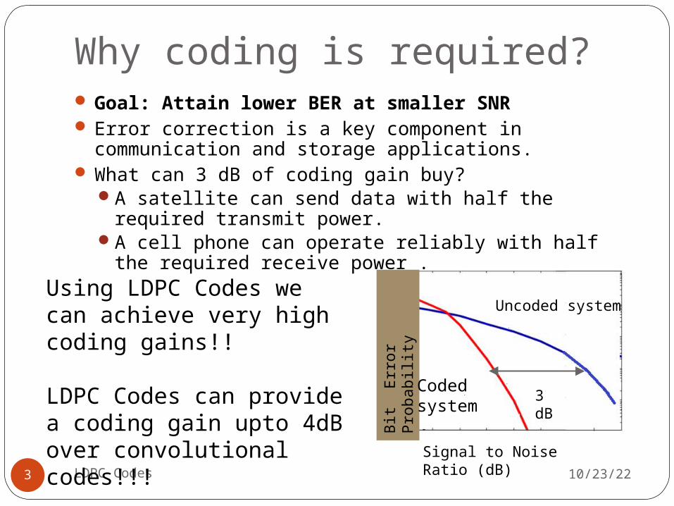
Goal: Attain lower BER at smaller SNR Error correction is a key component in communication and storage applications.

What can 3 dB of coding gain buy? A satellite can send data with half the required transmit power.

A cell phone can operate reliably with half the required receive power .

Bit

Error

Pr

obab

ilit

y

Signal to Noise Ratio (dB)

3 dB

Uncoded systemUsing LDPC Codes we can achieve very high coding gains!!

LDPC Codes can provide a coding gain upto 4dB over convolutional codes!!!

Coded system

10/23/22LDPC Codes4

Shannon Limit

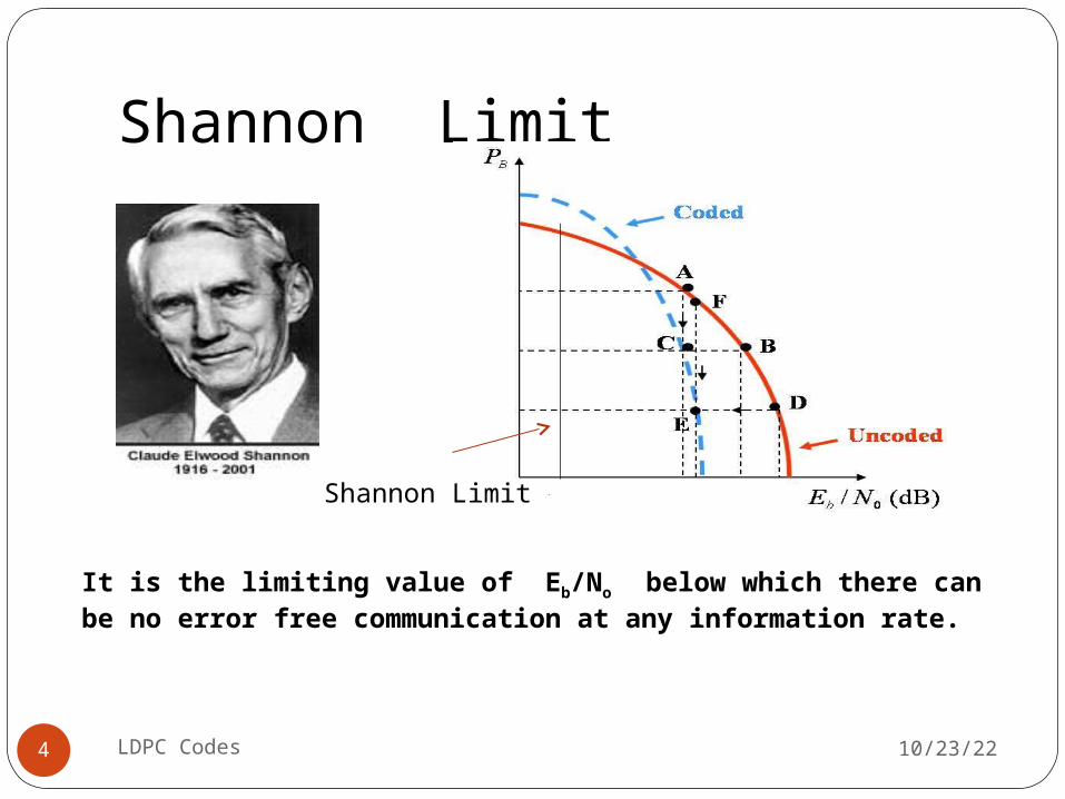
It is the limiting value of Eb/No below which there can be no error free communication at any information rate.

Shannon Limit

Performance of LDPC Codes

10/23/22LDPC Codes5

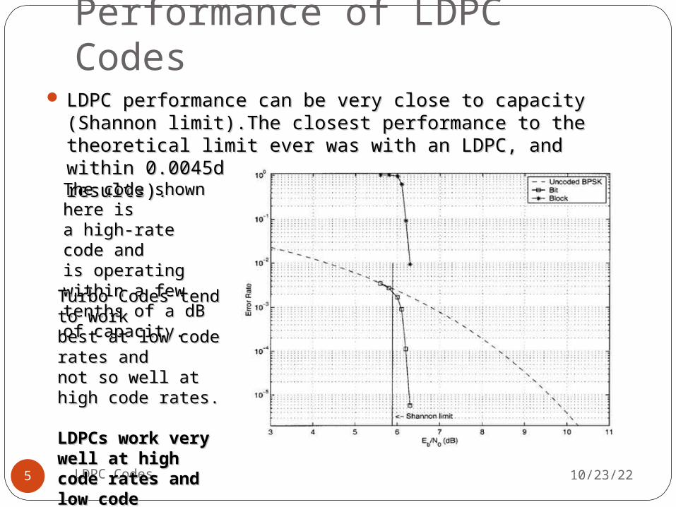
LDPC performance can be very close to capacity LDPC performance can be very close to capacity (Shannon limit).The closest performance to the (Shannon limit).The closest performance to the theoretical limit ever was with an LDPC, and theoretical limit ever was with an LDPC, and within 0.0045dB of capacity (experimental within 0.0045dB of capacity (experimental results).results).The code shown The code shown here ishere isa high-rate a high-rate code andcode andis operating is operating within a fewwithin a fewtenths of a dB tenths of a dB of capacity.of capacity.Turbo Codes tend Turbo Codes tend to workto workbest at low code best at low code rates andrates andnot so well at not so well at high code rates.high code rates.

LDPCs work very LDPCs work very well at high well at high code rates and code rates and low code low code rates!!!rates!!!

Do you Know??

10/23/22LDPC Codes6

The most powerful code currently known is a 1 million bit, rate ½, LDPC code achieving a capacity which is only 0.13dB from the

Shannon limit for a BER of 10-6.

Introduction

10/23/22LDPC Codes7

Low density parity check codes (LDPCs) are linear block codes that are characterized by a sparse-parity check matrix.

Originally introduced in 1963 by Robert Gallager, but were not widely studied for the next twenty years due to complex computations involved in processing long block lengths(n).

Tanner (1981) introduced the graphical representation of these codes.

After the introduction of turbo codes and the iterative decoding algorithm these codes were rediscovered by MacKay and Neal (1996) and MacKay (1999).

These codes are competitors to turbo codes in terms of performance and, if well designed, have better performance than turbo codes.

Main Characteristics of LDPC Codes

10/23/22LDPC Codes8

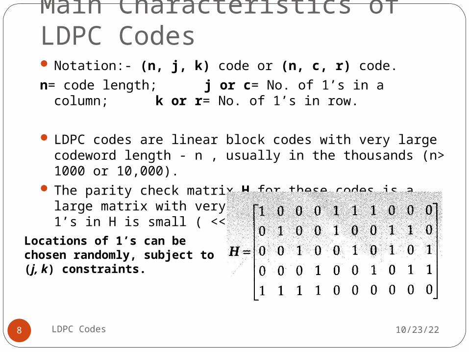
Notation:- (n, j, k) code or (n, c, r) code.n= code length; j or c= No. of 1’s in a column; k or r= No. of 1’s in row.

LDPC codes are linear block codes with very large codeword length - n , usually in the thousands (n> 1000 or 10,000).

The parity check matrix H for these codes is a large matrix with very few 1’s in it. Number of 1’s in H is small ( <<1%). Ex.(10,2,4) LDPC code

Locations of 1’s can be chosen randomly, subject to (j, k) constraints.

10/23/22LDPC Codes9

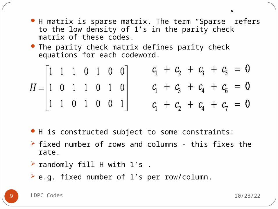
H matrix is sparse matrix. The term “Sparse” refers to the low density of 1’s in the parity check matrix of these codes.

The parity check matrix defines parity check equations for each codeword.

H is constructed subject to some constraints: fixed number of rows and columns - this fixes the rate.

randomly fill H with 1’s . e.g. fixed number of 1’s per row/column.

10/23/22LDPC Codes10

Depending on parity check matrix the LDPC codes are classified as –Regular and Irregular LDPC codes.

Rows and columns of regular LDPC code H matrix contains constant number of 1’s.

Irregular LDPC code is one in which the number of 1’s in rows and columns of H is not constant for all rows and columns.

Regular codes are easier to generate, whereas irregular codes with large code length have better performance.

If c is a codeword then c * HT =0.Code rate R= (1-j/k) or (1-c/r)


• Any two columns have an overlap of at most 1.This is done to increase dmin.

• Row column constraint(RC)-No two rows or columns may have more than one component in common.

• Sparseness of H can yield large minimum distance dmin as it allows us to avoid overlapping .

• Sparseness of H reduces decoding complexity. Sparsity is the key property that allows for the algorithmic efficiency.

Tanner Graph


A Tanner graph is a bipartite graph that describes the parity check matrix H.

Bipartite graph is an undirected graph whose nodes may be separated into two classes where edges only connect two nodes not residing in the same class.

There are two classes of nodes:Variable-nodes: Correspond to bits of the codeword or equivalently, to columns of the parity check matrix.There are n v-nodes.

Check-nodes: Correspond to parity check equations or equivalently, to rows of the parity check matrix. Also known as constraint nodes.There are m = (n-k) c-nodes.

Bipartite means that nodes of the same type cannot be connected (e.g. a c-node cannot be connected to another c-node)


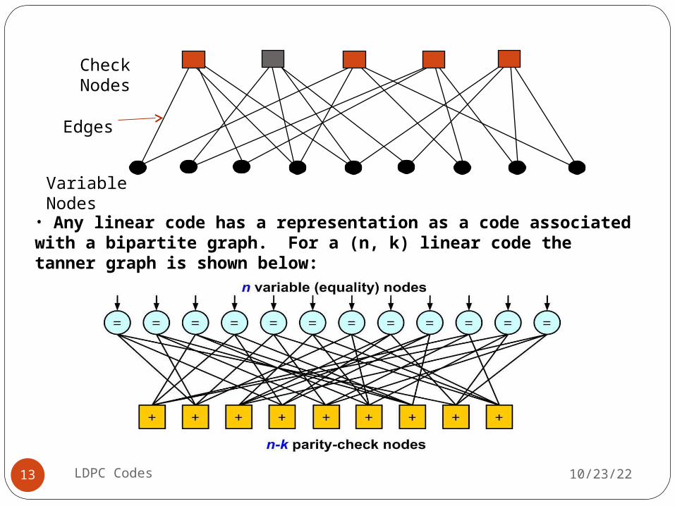
Check Nodes

Variable Nodes

Edges

• Any linear code has a representation as a code associated with a bipartite graph. For a (n, k) linear code the tanner graph is shown below:

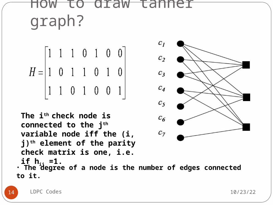
How to draw tanner graph?


The ith check node is connected to the jth variable node iff the (i, j)th element of the parity check matrix is one, i.e. if hij =1.• The degree of a node is the number of edges connected

to it.

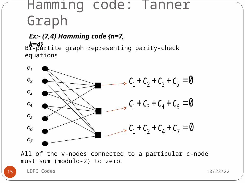
Hamming code: Tanner Graph


Bi-partite graph representing parity-check equations

05321 cccc

06431 cccc

07421 cccc

Ex:- (7,4) Hamming code {n=7, k=4}

All of the v-nodes connected to a particular c-node must sum (modulo-2) to zero.

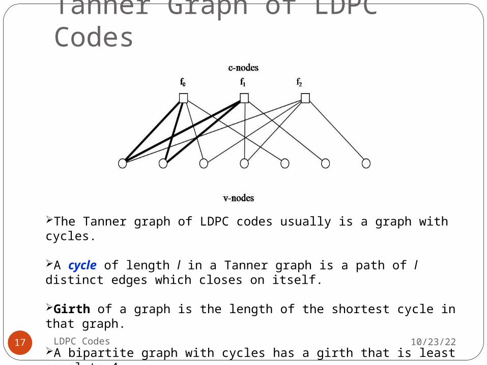
Tanner Graph of LDPC Codes


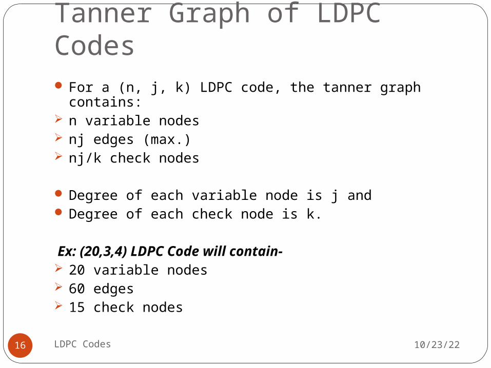
For a (n, j, k) LDPC code, the tanner graph contains:

n variable nodes nj edges (max.) nj/k check nodes

Degree of each variable node is j and Degree of each check node is k.

Ex: (20,3,4) LDPC Code will contain- 20 variable nodes 60 edges 15 check nodes

Tanner Graph of LDPC Codes


The Tanner graph of LDPC codes usually is a graph with cycles.

A cycle of length l in a Tanner graph is a path of l distinct edges which closes on itself.

Girth of a graph is the length of the shortest cycle in that graph.

A bipartite graph with cycles has a girth that is least equal to 4.

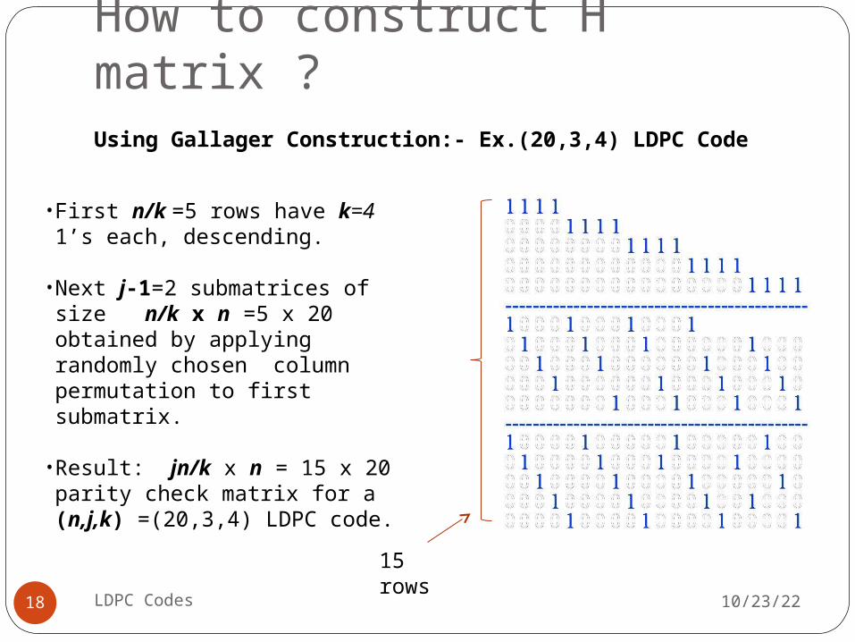
How to construct H matrix ?


Using Gallager Construction:- Ex.(20,3,4) LDPC Code

•First n/k =5 rows have k=4 1’s each, descending.

•Next j-1=2 submatrices of size n/k x n =5 x 20 obtained by applying randomly chosen column permutation to first submatrix.

•Result: jn/k x n = 15 x 20 parity check matrix for a (n,j,k) =(20,3,4) LDPC code.

15 rows

Encoding LDPC Codes


Problems with encoding:-Due to large dimensions of control matrix H, it is difficult to create generator matrix G.

For small n, G can be constructed using H but the H matrix of LDPC codes is not systematic.

A transformation of H into a systematic matrix Hsys is possible ( for ex. with the Gaussian elimination algorithm). Major drawback: the generator matrix Gsys of the systematic code is generally not sparse

The coding complexity increases rapidly in O(n2),which makes this operation too complex for usual length codes.

Encoding Complexity of LDPC Codes


Example: A (n, k)= (10000, 5000) LDPC code. The size of G is very large. c = xG= [x:xP] P is 5000 * 5000 matrix. We may assume that the density of 1's in P is 0.5

There are 12.5 * 106 1's in P. 12.5 * 106 addition (XOR) operations are required to encode one codeword!!!

For simplified encoding of LDPC code algebraic or geometric methods are used.

Encoding LDPC Codes (cont.)


Solution:-Direct encoding algorithms are used based on matrix H instead of generator matrix G.

Encoders are based on triangulation of control matrix H.

Steps: Preprocess parity check matrix H. The aim of the preprocessing is to put H as close as possible to upper triangulation form, using only permutations of rows or columns (but no algebraic operations).

Since this transformation was accomplished solely by permutations, the matrix is still sparse.

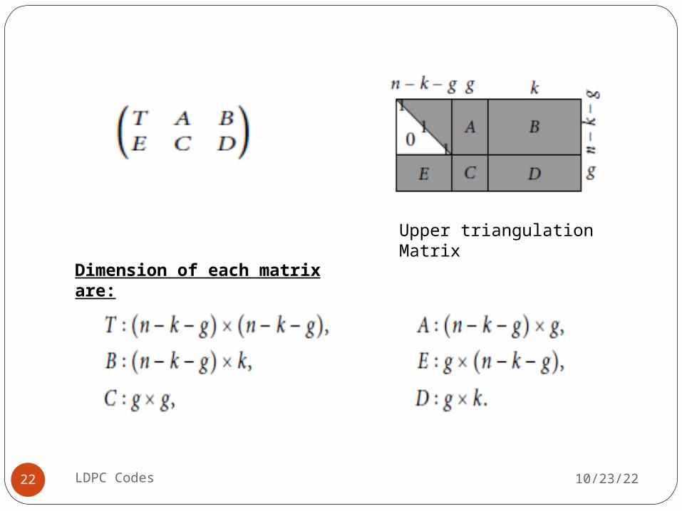
This matrix is made up of 6 sparse sub-matrices, denoted A,B,C,D,E and T .T is a upper triangular sub-matrix.


Upper triangulation Matrix

Dimension of each matrix are:


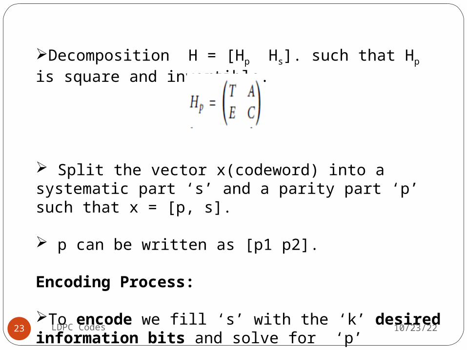
Decomposition H = [Hp Hs]. such that Hp is square and invertible.

Split the vector x(codeword) into a systematic part ‘s’ and a parity part ‘p’ such that x = [p, s].

p can be written as [p1 p2].

Encoding Process:

To encode we fill ‘s’ with the ‘k’ desired information bits and solve for ‘p’ using Hp pT = Hs sT.


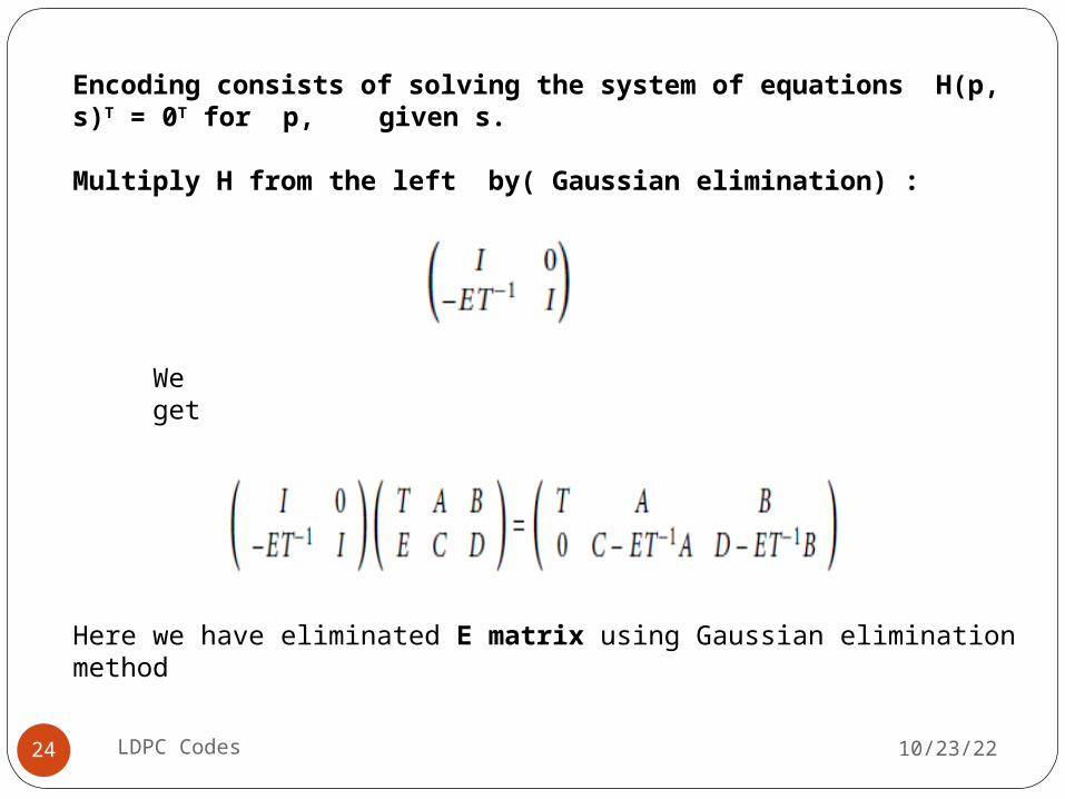
Encoding consists of solving the system of equations H(p, s)T = 0T for p, given s.

Multiply H from the left by( Gaussian elimination) :

We get

Here we have eliminated E matrix using Gaussian elimination method


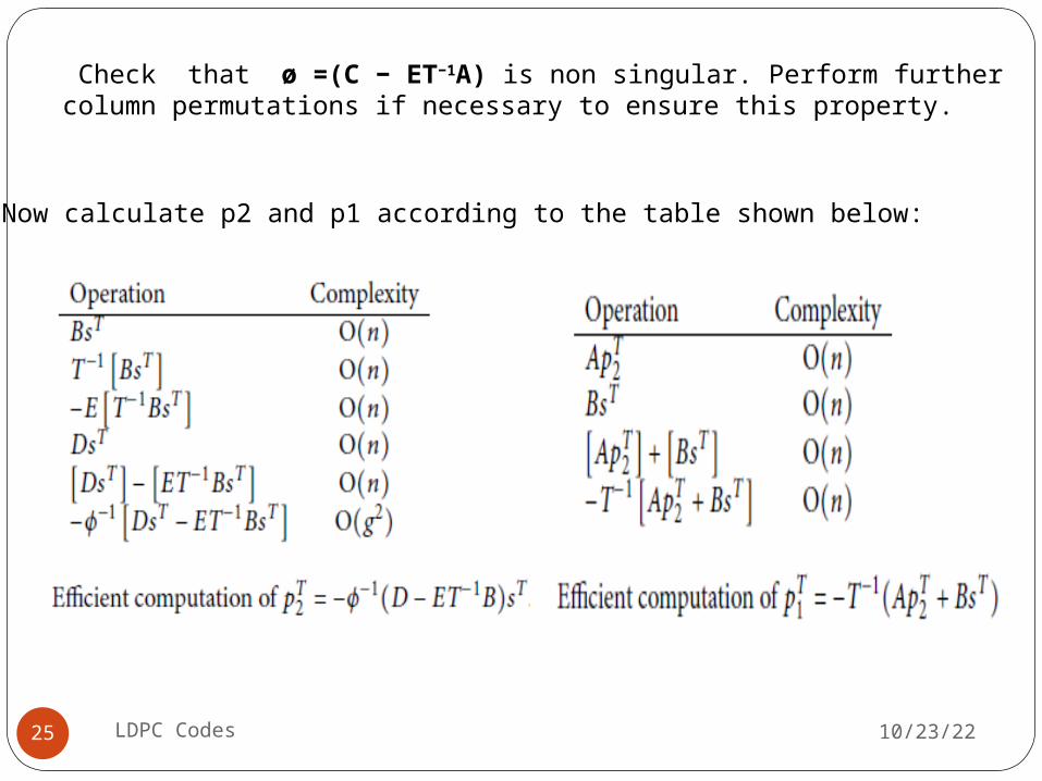
Check that ø =(C − ET−1A) is non singular. Perform further column permutations if necessary to ensure this property.

Now calculate p2 and p1 according to the table shown below:

Example


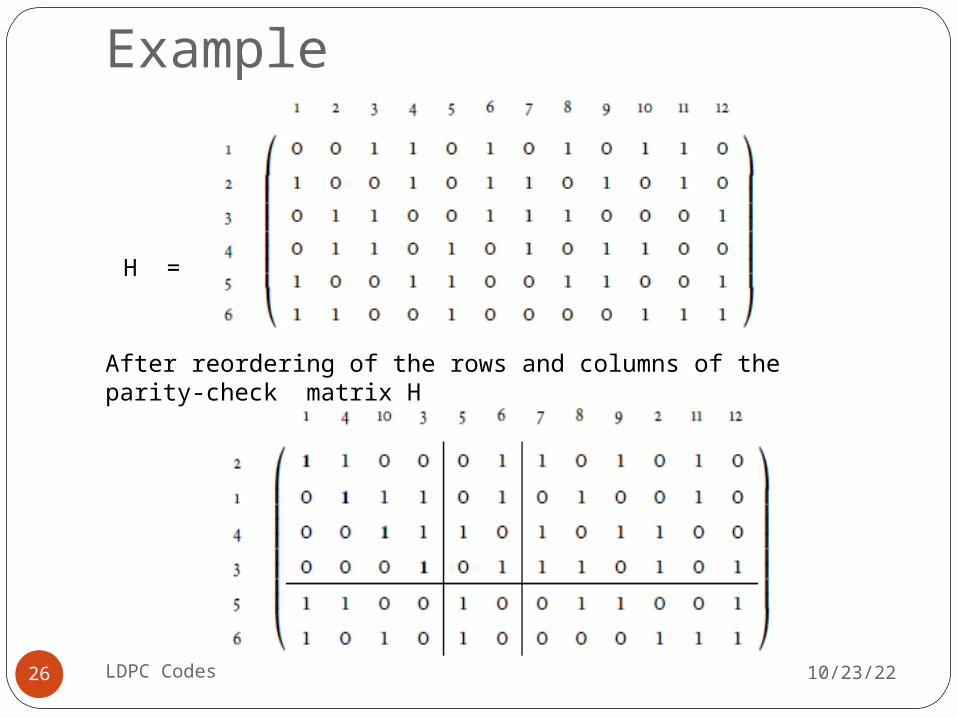
H =

After reordering of the rows and columns of the parity-check matrix H


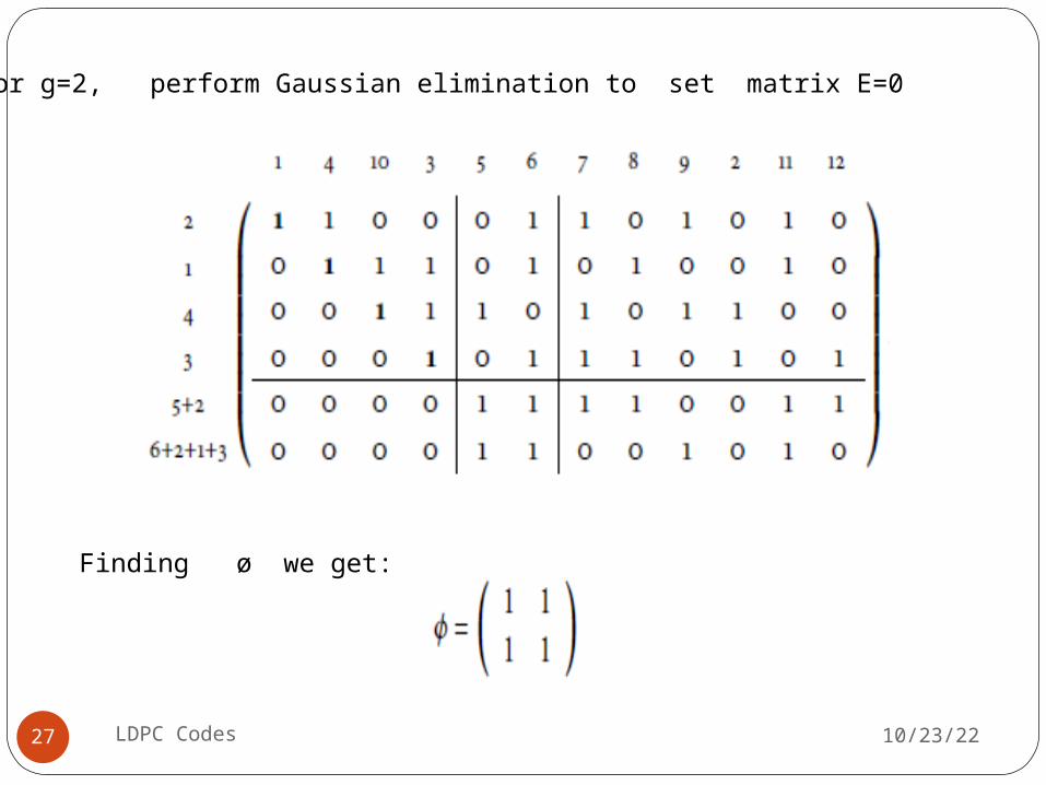
For g=2, perform Gaussian elimination to set matrix E=0

Finding ø we get:


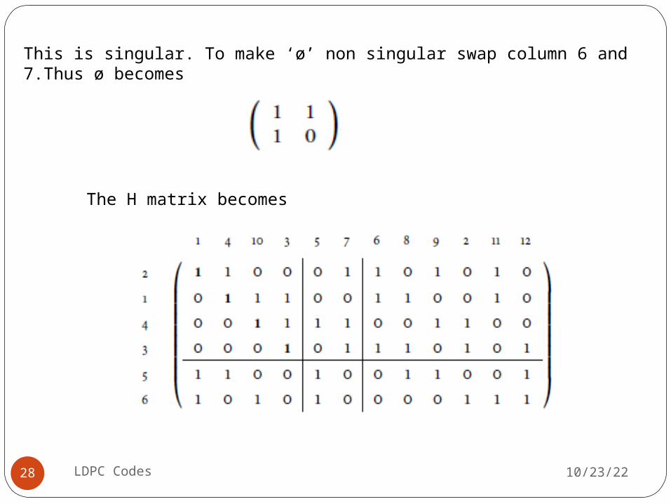
This is singular. To make ‘ø’ non singular swap column 6 and 7.Thus ø becomes

The H matrix becomes


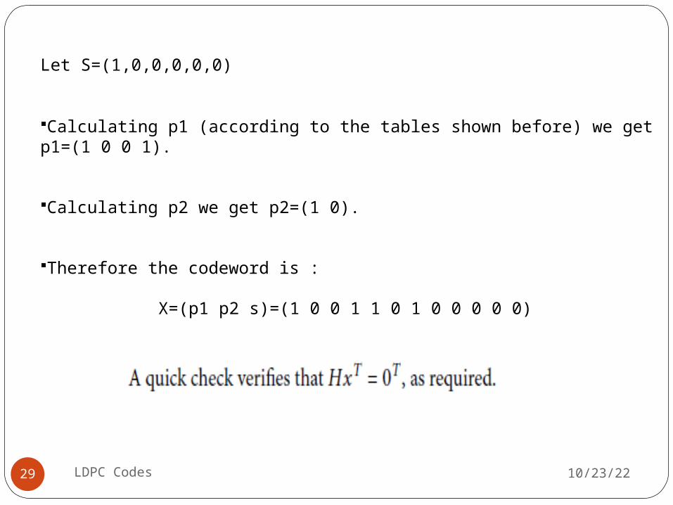
Let S=(1,0,0,0,0,0)

Calculating p1 (according to the tables shown before) we get p1=(1 0 0 1).

Calculating p2 we get p2=(1 0).

Therefore the codeword is :

X=(p1 p2 s)=(1 0 0 1 1 0 1 0 0 0 0 0)

Decoding of LDPC Codes


Performance of Error Control Codes (ECC) strongly depends on decoding process.

Iterative decoding algorithms are used .These iterative algorithms perform sequential repair of erroneous bits instead of searching for closest codeword in code space.

Decoding will be done in an iterative way: iterate between variable (bit) nodes and checks nodes.

Like Turbo codes, LDPC can be decoded iteratively– Instead of a trellis, the decoding takes place on a

Tanner graph.– Messages are exchanged between the v-nodes and c-nodes.

– Edges of the graph act as information pathways.

Decoding Algorithms


Graph based algorithms: Sum-product algorithm for general graph based codes. MAP(BCJR) algorithm for trellis graph based codes Message passing algorithm for bipartite graph based codes.

Hard decision decoding algorithms: Simpler decoder construction . Faster convergence. Ex: Bit flipping algorithm, Viterbi algorithm.

Soft Decision decoding algorithms: Complicated decoder construction Slow convergence. Ex: (iterative algorithm)-message passing algorithm /belief propagation algorithm

Bit Flipping Algorithm-Example


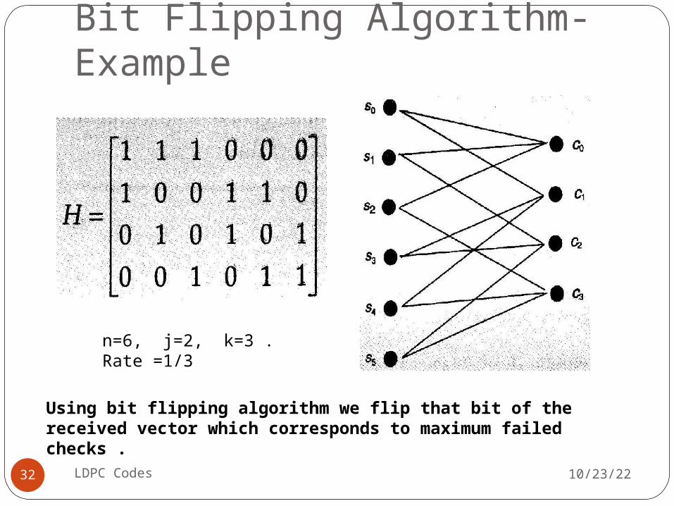
n=6, j=2, k=3 . Rate =1/3

Using bit flipping algorithm we flip that bit of the received vector which corresponds to maximum failed checks .


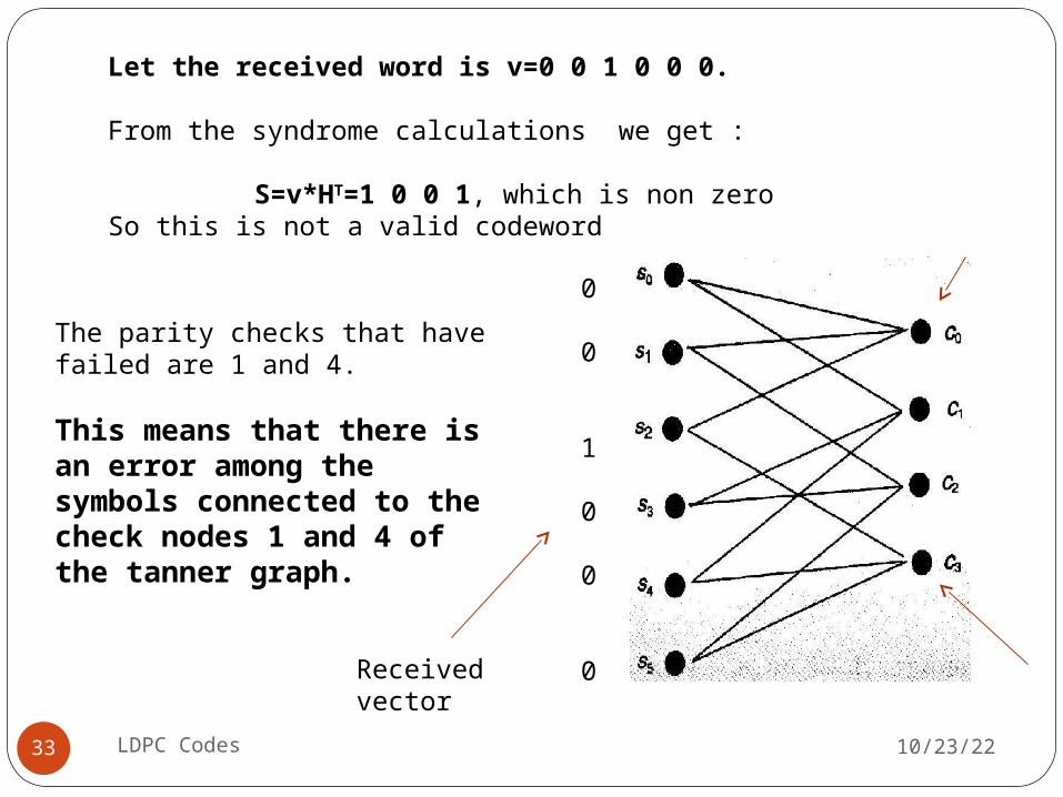
Let the received word is v=0 0 1 0 0 0.

From the syndrome calculations we get :

S=v*HT=1 0 0 1, which is non zeroSo this is not a valid codeword

The parity checks that have failed are 1 and 4.

This means that there is an error among the symbols connected to the check nodes 1 and 4 of the tanner graph.

0

0

1

0

0

0Received vector


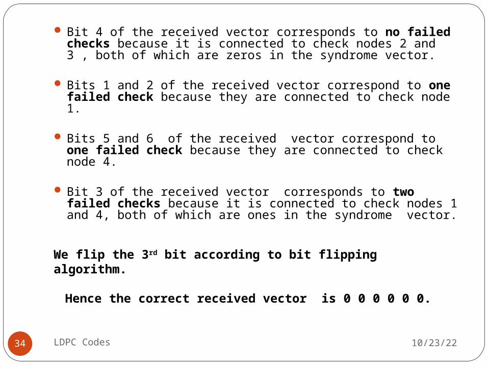
Bit 4 of the received vector corresponds to no failed checks because it is connected to check nodes 2 and 3 , both of which are zeros in the syndrome vector.

Bits 1 and 2 of the received vector correspond to one failed check because they are connected to check node 1.

Bits 5 and 6 of the received vector correspond to one failed check because they are connected to check node 4.

Bit 3 of the received vector corresponds to two failed checks because it is connected to check nodes 1 and 4, both of which are ones in the syndrome vector.

We flip the 3rd bit according to bit flipping algorithm.

Hence the correct received vector is 0 0 0 0 0 0.

Message Passing Algorithm


Important Points:Information is transferred from variable to check nodes and from check to variable nodes along edges of the tanner graph at discrete points of time.

Initially every variable node has a message assigned to it. These messages can be probabilities coming directly from the received vector.

At time 1, some or all variable nodes send the message assigned to them to all attached check nodes via the edges of the graph.

At time 2, some of those check nodes that received a message process the message and send along a message to some or all variable nodes attached to them.

These two transmissions of messages make up one iteration. The process continues through several iterations.


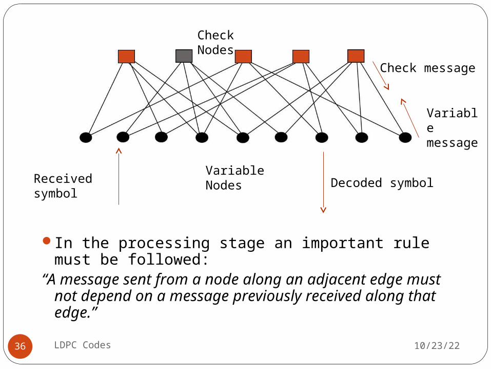
In the processing stage an important rule must be followed:

“A message sent from a node along an adjacent edge must not depend on a message previously received along that edge.”

Check Nodes

Variable Nodes

Check message

Variable message

Received symbol

Decoded symbol

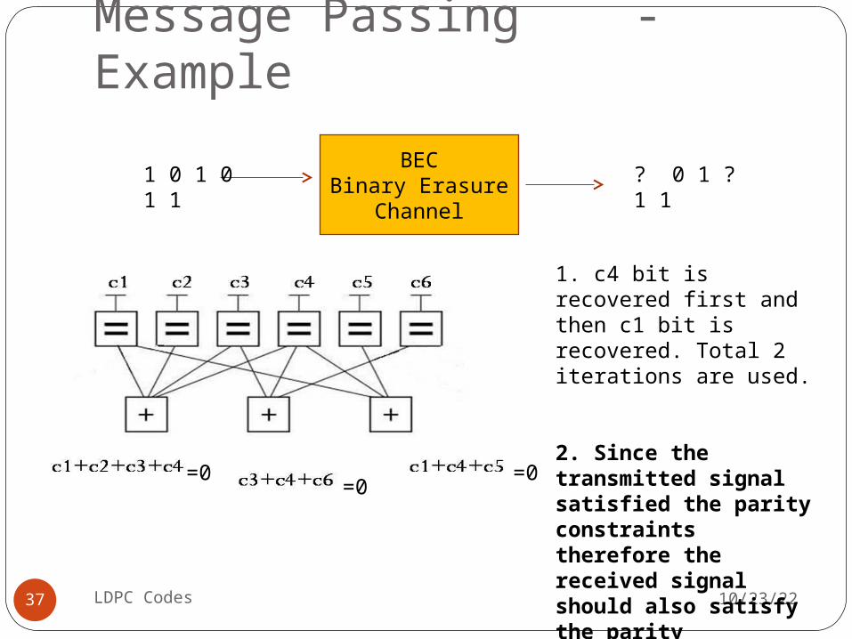
Message Passing - Example


BECBinary Erasure

Channel1 0 1 0 1 1

? 0 1 ? 1 1

1. c4 bit is recovered first and then c1 bit is recovered. Total 2 iterations are used.

2. Since the transmitted signal satisfied the parity constraints therefore the received signal should also satisfy the parity constraint.

=0 =0=0

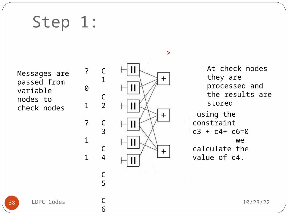
Step 1:


C1

C2

C3

C4

C5

C6

?

0

1

?

1

1

Messages are passed from variable nodes to check nodes

At check nodes they are processed and the results are stored

using the constraint c3 + c4+ c6=0 we calculate the value of c4.

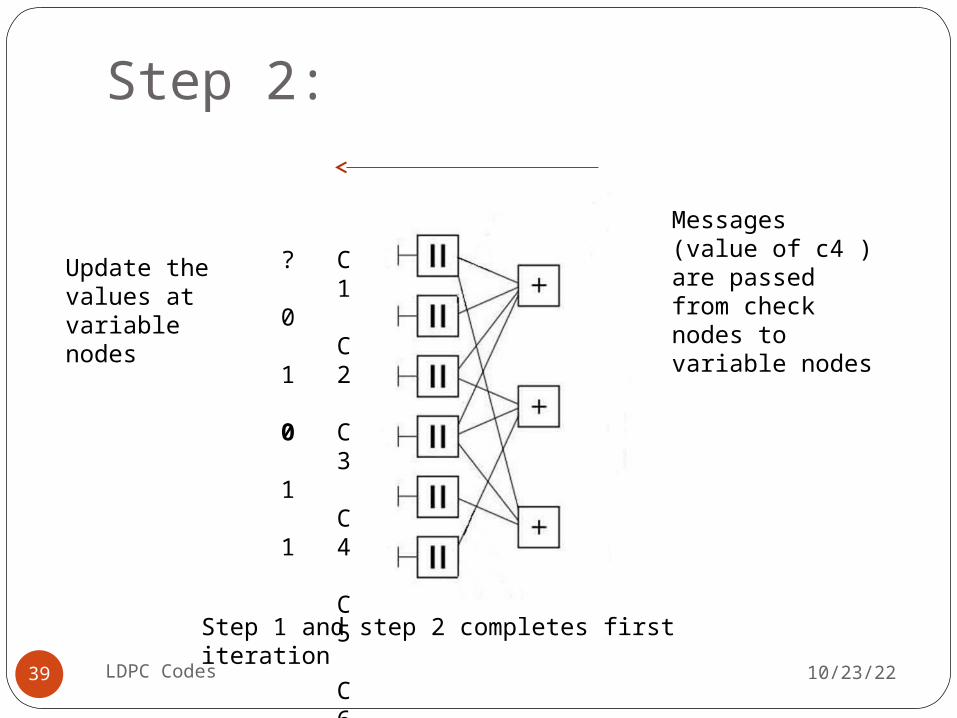
Step 2:


C1

C2

C3

C4

C5

C6

Messages (value of c4 ) are passed from check nodes to variable nodes

?

0

1

0

1

1

Update the values at variable nodes

Step 1 and step 2 completes first iteration

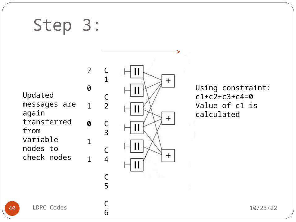
Step 3:


C1

C2

C3

C4

C5

C6

?

0

1

0

1

1

Updated messages are again transferred from variable nodes to check nodes

Using constraint: c1+c2+c3+c4=0Value of c1 is calculated

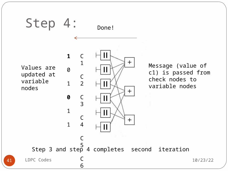
Step 4:


C1

C2

C3

C4

C5

C6

Message (value of c1) is passed from check nodes to variable nodes

1

0

1

0

1

1

Values are updated at variable nodes

Done!

Step 3 and step 4 completes second iteration


For other channel models, the message passed between the variable nodes and check nodes are real numbers ,which express probabilities and likelihoods of belief.

If messages are in the form of belief or probabilities instead of hard values 1 or 0, then it is known as belief propagation algorithm.

Applications of LDPC Codes


Deep space communications WiMaxDVBDABUMTSMultimedia Applications

References


Books:• Digital Communications-Bernard Sklar• Information Theory Coding and Cryptography-Ranjan Bose

• Digital Communications-Simon Haykin• Modern Analog and Digital Communications-B.P.Lathi• Modern Coding Theory-Richardson-Urbanke• Codes and Turbo Codes-Claude Berrou

Papers: R. Gallager, “Low-density parity-check codes" ,IRE Trans. Information Theory, pp. 21-28, January1962.

• LDPC Codes: An Introduction - Amin Shokrollahi, Digital Fountain, Inc.

• LDPC Codes – a brief Tutorial- Bernhard M.J. Leiner• Parallel Decoding Architectures for Low Density Parity Check Codes - C. Howlarid aizd A. Blaiiksby, High Speed Communications VLSI Research Department.

ldpc codes

Documents