food webs and carbon flux in the barents sea
TRANSCRIPT

Progress in Oceanography 71 (2006) 232–287
www.elsevier.com/locate/pocean
Progress inOceanography
Food webs and carbon flux in the Barents Sea
Paul Wassmann a,*, Marit Reigstad a, Tore Haug b, Bert Rudels c,Michael L. Carroll e, Haakon Hop d, Geir Wing Gabrielsen d, Stig Falk-Petersen d,Stanislav G. Denisenko g, Elena Arashkevich f, Dag Slagstad a,h, Olga Pavlova d
a Norwegian College of Fishery Science, University of Tromsø, N-9037 Tromsø, Norwayb Institute of Marine Research, Tromsø Branch, P.O. Box 6404, N-9294 Tromsø, Norway
c Institute of Marine Research, P.O. Box 2, FI-00561 Helsinki, Finlandd Norwegian Polar Institute, N-9296 Tromsø, Norway
e Akvaplan-niva, N-9296 Tromsø, Norwayf Shirshov Institute of Oceanology, Academy of Sciences of Russia, Nakhimovsky Avenue 36, 117851 Moscow, Russia
g Zoological Institute, Russian Academy of Sciences, 199034 St. Petersburg, Russiah SINTEF Fisheries and Aquaculture, N-7465 Trondheim, Norway
Available online 13 November 2006
Abstract
Within the framework of the physical forcing, we describe and quantify the key ecosystem components and basic foodweb structure of the Barents Sea. Emphasis is given to the energy flow through the ecosystem from an end-to-end perspec-tive, i.e. from bacteria, through phytoplankton and zooplankton to fish, mammals and birds. Primary production in theBarents is on average 93 g C m�2 y�1, but interannually highly variable (±19%), responding to climate variability andchange (e.g. variations in Atlantic Water inflow, the position of the ice edge and low-pressure pathways). The traditionalfocus upon large phytoplankton cells in polar regions seems less adequate in the Barents, as the cell carbon in the pelagic ismost often dominated by small cells that are entangled in an efficient microbial loop that appears to be well coupled to thegrazing food web. Primary production in the ice-covered waters of the Barents is clearly dominated by planktonic algaeand the supply of ice biota by local production or advection is small. The pelagic–benthic coupling is strong, in particularin the marginal ice zone. In total 80% of the harvestable production is channelled through the deep-water communities andbenthos. 19% of the harvestable production is grazed by the dominating copepods Calanus finmarchicus and C. glacialis inAtlantic or Arctic Water, respectively. These two species, in addition to capelin (Mallotus villosus) and herring (Clupea
harengus), are the keystone organisms in the Barents that create the basis for the rich assemblage of higher trophic levelorganisms, facilitating one of the worlds largest fisheries (capelin, cod, shrimps, seals and whales). Less than 1% of theharvestable production is channelled through the most dominating higher trophic levels such as cod, harp seals, minkewhales and sea birds. Atlantic cod, seals, whales, birds and man compete for harvestable energy with similar shares. Cli-mate variability and change, differences in recruitment, variable resource availability, harvesting restrictions and manage-ment schemes will influence the resource exploitation between these competitors, that basically depend upon the efficientenergy transfer from primary production to highly successful, lipid-rich zooplankton and pelagic fishes.� 2006 Elsevier Ltd. All rights reserved.
0079-6611/$ - see front matter � 2006 Elsevier Ltd. All rights reserved.
doi:10.1016/j.pocean.2006.10.003
* Corresponding author. Tel.: +47 776 44459; fax: +47 776 46020.E-mail address: [email protected] (P. Wassmann).
P. Wassmann et al. / Progress in Oceanography 71 (2006) 232–287 233
1. Introduction
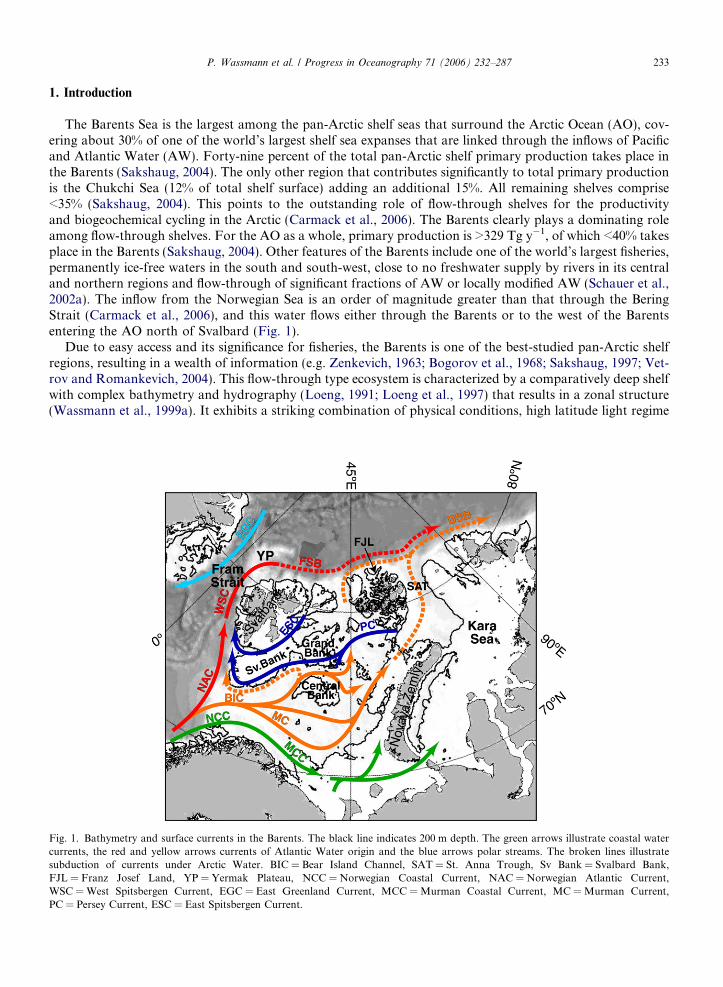
The Barents Sea is the largest among the pan-Arctic shelf seas that surround the Arctic Ocean (AO), cov-ering about 30% of one of the world’s largest shelf sea expanses that are linked through the inflows of Pacificand Atlantic Water (AW). Forty-nine percent of the total pan-Arctic shelf primary production takes place inthe Barents (Sakshaug, 2004). The only other region that contributes significantly to total primary productionis the Chukchi Sea (12% of total shelf surface) adding an additional 15%. All remaining shelves comprise<35% (Sakshaug, 2004). This points to the outstanding role of flow-through shelves for the productivityand biogeochemical cycling in the Arctic (Carmack et al., 2006). The Barents clearly plays a dominating roleamong flow-through shelves. For the AO as a whole, primary production is >329 Tg y�1, of which <40% takesplace in the Barents (Sakshaug, 2004). Other features of the Barents include one of the world’s largest fisheries,permanently ice-free waters in the south and south-west, close to no freshwater supply by rivers in its centraland northern regions and flow-through of significant fractions of AW or locally modified AW (Schauer et al.,2002a). The inflow from the Norwegian Sea is an order of magnitude greater than that through the BeringStrait (Carmack et al., 2006), and this water flows either through the Barents or to the west of the Barentsentering the AO north of Svalbard (Fig. 1).
Due to easy access and its significance for fisheries, the Barents is one of the best-studied pan-Arctic shelfregions, resulting in a wealth of information (e.g. Zenkevich, 1963; Bogorov et al., 1968; Sakshaug, 1997; Vet-rov and Romankevich, 2004). This flow-through type ecosystem is characterized by a comparatively deep shelfwith complex bathymetry and hydrography (Loeng, 1991; Loeng et al., 1997) that results in a zonal structure(Wassmann et al., 1999a). It exhibits a striking combination of physical conditions, high latitude light regime
Fig. 1. Bathymetry and surface currents in the Barents. The black line indicates 200 m depth. The green arrows illustrate coastal watercurrents, the red and yellow arrows currents of Atlantic Water origin and the blue arrows polar streams. The broken lines illustratesubduction of currents under Arctic Water. BIC = Bear Island Channel, SAT = St. Anna Trough, Sv Bank = Svalbard Bank,FJL = Franz Josef Land, YP = Yermak Plateau, NCC = Norwegian Coastal Current, NAC = Norwegian Atlantic Current,WSC = West Spitsbergen Current, EGC = East Greenland Current, MCC = Murman Coastal Current, MC = Murman Current,PC = Persey Current, ESC = East Spitsbergen Current.
234 P. Wassmann et al. / Progress in Oceanography 71 (2006) 232–287
and substantial advection of heat, salt, nutrients and biomass by the Norwegian Atlantic Current (NAC; e.g.Adlandsvik and Loeng, 1991; Sakshaug et al., 1995). Sea ice can cover up to 90% of the Barents Sea surface inwinter, but there is no locally produced multi-year ice (MYI) (Vinje and Kvambek, 1991). Thus, much of theBarents experiences ablation and growth of sea ice on a seasonal basis, the seasonal ice zone (SIZ). The mar-ginal ice zone (MIZ), i.e. the transition between ice-covered and ice-free SIZ, crosses most of the shelf duringthe northbound progression of the spring bloom and is of particular importance to the production of organicmatter (Sakshaug and Skjoldal, 1989).
Russian scientists intensively investigated plankton and benthos communities of the Barents, in particularin the first half of 20th century (e.g. Linko, 1907; Jashnov, 1939; Zelikman and Kamshilov, 1960; Zenkevich,1963). Over the last 40 years, systems ecological baseline research has primarily focused upon hydrodynamics,productivity, plankton and the biological basis for one of the world’s largest fisheries. Degtereva (1973), Dru-zhkov and Makarevich (1992), Makarevich and Larionov (1992) and Timofeev (1997) presented summaries ofthe Russian plankton work. Between 1984–1990 (Pro Mare) and 1998–2000 (ALV), the Norwegian ResearchCouncil supported system-wide ecological programmes that focused upon the southwestern and central regionof the Barents (e.g. Sakshaug et al., 1991; Wassmann, 2002, respectively). Based upon the physical, chemicaland biological oceanographic knowledge, the seasonal and interannual dynamics of carbon flux of the Barentshave been modelled (Wassmann and Slagstad, 1993; Slagstad and Wassmann, 1997; Slagstad and McClimans,2005; Wassmann et al., 2006).
The Barents plays a crucial role in Norwegian and Russian fisheries and aquaculture. That is the founda-tion for the extensive investigations of economically important stocks of fish and mammals in the region andtheir food consumption (e.g. Hamre, 1994; Gjøsæter, 1995; Bogstad et al., 2000). However, except for thehyperbenthic shrimp Pandalus borealis, our knowledge of benthos has expanded less rapidly, despite some fineRussian investigations (e.g. Zenkevich, 1963). Also sea birds are well studied in the Barents region (e.g. Barrettet al., 2001). However, the smaller planktonic forms and ice fauna/flora, as well as the pelagic–benthic cou-pling, are less well known and deserve more consideration.
The goal of this publication is to present an end-to-end overview of key players in the food web of theBarents. We also present some of the basic dynamics of the Barents ecosystem by summarizing the most recentknowledge of physical oceanography, plankton and ice-biota, but also information on pelagic–benthic cou-pling, benthos, fishes, mammals and seabirds. Some emphasis is given to earlier investigations and Russianwork that may be inadequately known to the international reader. The ultimate goal is to portray the key ele-ments of the food web in concert and to construct a carbon budget that indicates how the productivity in theBarents is channelled through the various food web compartments.
2. Bathymetry, water mass distribution and circulation
The Barents is the largest (1.6 · 106 km2) and the deepest (mean depth 230 m) of the AO shelf seas(Carmack et al., 2006) and has a complex bathymetry. Extensive shallow areas are found, especially westand southwest of Novaja Zemlja and around Svalbard, as well as large, isolated banks, the Central Bank,the Great Bank and the Svalbard Bank (Fig. 1). Deeper troughs, the Bear Island Channel and the VictoriaChannel, and depressions separate these deeper banks, the Hopen Deep in the west and the southeast andnortheast basins in the east. The Barents is not just a shelf sea; it is also a major passage for waters fromthe Norwegian Sea entering the AO, i.e. a flow-through shelf (Carmack et al., 2006). The effective silldepth is around 230 m. The large expanse of the Barents allows for a much stronger transformation ofthe entering waters than in the deeper passage to the west through Fram Strait. In contrast to Fram Strait(characterized by extensive recirculation), the Barents is essentially a one-way passage only permittingwater to enter the AO. However, the inflow is not strong enough to flood the entire Barents shelf, andit is mainly confined to the south. In the northern part, the upper layer comprises less saline and lessdense Arctic Waters (ArW) partly originating from the AO. The boundary between these waters consti-tutes the Polar Front (PF), which runs along the eastern slope of the Svalbard Bank and then eastwardfrom Hopen towards Novaja Zemlja. The PF is always south of the Grand Bank, while it meanders backand forth across the Central Bank, leaving ‘‘Arctic’’ water above the Central Bank as an isolated cold lens(Fig. 1).
P. Wassmann et al. / Progress in Oceanography 71 (2006) 232–287 235
The description of the physical oceanography in the Barents is largely based upon Tantsiura (1959) andLoeng (1991, 1992). The inflow from the Norwegian Sea takes place through the Bear Island Channel. Closeto the coast the low salinity (S � 34.4 pss) water of the Norwegian Coastal Current (NCC) carries a substan-tial fraction of the runoff from the Baltic and the Norwegian coasts into the southern Barents (Fig. 1). It con-tinues eastward as the Murman Coastal Current. Additional low salinity water is added as it passes theentrance to the White Sea and the mouth of the Pechora River, so the salinity remains low (S = 34.6 pss).Most of this ‘‘coastal’’ water passes into the Kara Sea through the Kara Gate. River runoff and net precip-itation are small, and the NCC is the major freshwater source for the Barents.
AW (S > 35.0 pss) comprises the main part of the inflow. The NAC splits to the west of the Bear IslandChannel (Fig. 1). One part continues northward as the West Spitsbergen Current (WSC), while the rest entersthe Barents as the North Cape Current in the deeper part of the Bear Island Channel, to the north of the NCC.The inflow forms three branches in the Barents. Two branches flow eastward, south of the Central Bank,where they finally merge once again, creating the Murman Current. The third branch moves northward tothe west of the Central Bank into the Hopen Deep. This branch splits in the northern part of the Hopen Deep.One part turns eastward, following the anticyclonic circulation around the Central Bank before entering theeastern basins. A smaller fraction crosses the sill between Edgeøya and the Grand Bank, contributing to thebottom waters in the northern basins (Pfirman et al., 1994). The rest recirculates and returns to the NorwegianSea as cooled, denser AW south of Bjørnøya. The return flow does not appear to extend smoothly up thesoutheastern slope of the Svalbard Bank. Above the 250 m isobath a northward flowing jet has been observed(Li, 1995; Loeng and Sætre, 2001), lying between the returning AW and the ArW on the Svalbard Bank. TheAW that penetrates to the eastern Barents flows northeast adjacent to Novaja Zemlja and eventually enters theAO, primarily passing through the strait between Novaja Zemlja and Franz Josef Land and then down the St.Anna Trough (Midttun, 1985; Rudels, 1987; Loeng et al., 1993).
In the northern Barents, the upper layers are dominated by less saline (S � 34.6 pss) ArW, entering partlyfrom the AO but mainly from the Kara Sea, passing south of Franz Josef Land (Loeng, 1991). The PerseyCurrent then carries the ArW westward along the PF (Fig. 1). A small fraction is detached southward tothe Central Bank but the main part continues to the Svalbard Bank, where it veers to southwest and movesas the Bear Island Current along the southeastern slope of the Svalbard Bank to Bjørnøya (Tantsiura, 1959).This current follows the 100 m isobath, shallower than the aforementioned northward moving jet of AW.
As the ArW reaches Bjørnøya, it is carried with the WSC northward along the western edge of SvalbardBank (Fig. 1). As the WSC reaches Svalbard it becomes further augmented by the Sørkapp Current (extensionof the East Spitsbergen Current), which brings low salinity waters from the AO around Svalbard to FramStrait. The WSC thus transports the ArW back into the AO through Fram Strait, and little net flow fromthe AO to the Norwegian Sea takes place over the Barents.
2.1. Inflow of Atlantic Water
Early estimates of the inflow between Norway and Bjørnøya, around 1 Sv, were based on budget consid-erations (Aagaard and Greisman, 1975), balance arguments (Rudels, 1987), and other indirect methods (Nik-iforov and Shpaiker, 1980). The first current measurements between Bjørnøya and Norway were made in 1978and indicated an inflow of around 3 Sv and a return flow of cooled AW of about 1.2 Sv, giving a net inflow of1.8 Sv (Blindheim, 1989).
After 1997, direct current measurements have been made continuously between Norway and Bjørnøya. Theflow of AW is mainly barotropic and displays large, short-term variations with monthly mean transports rang-ing from more than 5 Sv into and almost 5 Sv out of the Barents (Ingvaldsen et al., 2004a,b). The mean nettransport is about 1.5 Sv into the Barents, and the flow is stronger in winter than in summer, 1.7 vs. 1.3 Sv,respectively. The lower transport in summer is attributed to the predominately northeasterly winds, which leadto a northward Ekman transport. This lowers the sea level at the Norwegian coast, and the smaller sea levelslope leads to a weaker inflow. This is confirmed by the distribution of the NCC water, which in summer isencountered at the surface across almost the entire passage. In winter, the winds are mainly from southwestand the along-section Ekman transport is towards the Norwegian coast. The increased sea level slope adds tothe barotropic transport into the Barents, and the coastal water becomes confined in a narrow wedge close to
236 P. Wassmann et al. / Progress in Oceanography 71 (2006) 232–287
the coast. The period of strong net outflow mostly occurs in April, when the wind direction changes fromsouthwest to north – northeast (Ingvaldsen et al., 2004b). There is however, considerable difference betweenthe modelled and measured flux estimates, with deviations up to 1 Sv for the inflow in July and August, prob-ably due to inadequate spatial coverage of current meters (Slagstad and McClimans, 2005).
The transport in the NCC must be assessed separately and be added to the Atlantic inflow. Most estimateslie around 0.7–0.8 Sv (Rudels, 1987; Blindheim, 1989). This implies that 2.2–2.3 Sv could enter the AO overthe Barents, mainly passing down the St. Anna Trough. The only current measurements available from thepassage between Novaja Zemlja and Franz Josef Land were made in 1991, and indicated a net transport of2 Sv from the Barents into the Kara Sea, roughly balancing the inflow from the Norwegian Sea (Loenget al., 1993, 1997; Schauer et al., 2002a).
2.2. Stratification and brine formation
Heat loss in the Barents is large, causing extensive transformations of the waters entering from the south-west. The AW is cooled significantly in the Hopen Deep and in the eastern basins. However, the largest trans-formations occur over shallow areas, west of Novaja Zemlja and over the Central Bank, and in Storfjorden(Nansen, 1906; Midttun, 1985; Anderson et al., 1988; Quadfasel et al., 1988; Schauer, 1995).
Lee polynyas are frequently observed to the west of Novaja Zemlja. The open water leads to extensive iceformation, brine rejection and haline convection that eventually reaches the bottom. Nansen (1906) first sug-gested such a process. Defant (1949, 1961) described the cooling of the upper part of the water column tofreezing, leading to brine rejection and convection, eventually reaching the bottom. The continuous rejectionof brine causes an increase in salinity and density of the bottom water throughout the winter. The dense watersinks into the neighbouring deeper depressions, entrains ambient water and continues northward, mainly intothe Kara Sea and via the St. Anna Trough into the AO. A smaller fraction reaches the AO via the VictoriaChannel. This flow of cold, dense bottom water in the channel has been followed along the continental slopenorthwest of Franz Josef Land (Rudels, 1986; Schauer et al., 1997; Rudels and Friedrich, 2000). The St. Annaoutflow is much stronger, comprising not only of dense bottom water but also of transformed AW. It is strat-ified and forms a water column over the continental slope dense enough to penetrate down to 1200–1500 m.As this Barents Sea inflow branch enters the Arctic Ocean east of St. Anna Trough, it displaces the Fram Straitinflow branch offshore, leading to strong, isopycnal mixing between the two branches (Rudels et al., 1994;Schauer et al., 1997, 2002b).
The Persey Current feeds low salinity ArW and sea ice to the Central Bank, creating strong stability and asurface layer that can be cooled to freezing temperature in winter before overturning. This leads to ice forma-tion and brine rejection. The density in the upper layer increases, and the ensuing convection eventually pen-etrates into the underlying water and finally to the bottom. A cold, dense water column, less saline than theAW, is created and remains as a Taylor column on the bank, enforcing the anti-cyclonic circulation aroundthe bank (Quadfasel et al., 1992). Bottom friction causes a slow draining of the Taylor column down the slopeof the bank into the Hopen Deep and into the eastern basins. The dense water sinking into the Hopen Deeppenetrates to the bottom, leaves the Barents through the Bear Island Channel and sinks down the continentalslope into the Norwegian Sea (Blindheim, 1989; Quadfasel et al., 1992).
Extensive ice formation, brine rejection in winter and the subsequent melting of the ice in summer lead to aseparation of the water column into a colder and denser deep-water, and a less saline, less dense upper layer.The low salinity surface water contributes, together with the inflows from the AO and the Kara Sea, to main-tain stable stratification in the northern and eastern Barents.
Outside the polynya areas the stability of the water column limits the convection to depths above thepycnocline and a cold (freezing point) mixed layer with salinity of 34.5–34.6 pss reforms each winter. The win-ter-homogenised upper layer, especially that created in the eastern Barents, can, by joining the St. Anna out-flow, contribute to the AO halocline (Rudels et al., 2004). This formation mechanism is similar to the onesuggested by Rudels et al. (1996) for the Fram Strait branch contribution to the halocline – a less saline surfacelayer, initially created by sea ice melting above warmer water or by seasonal ice melt in summer, becomeshomogenised by brine rejection and haline convection in winter. Its salinity and density increase, but itremains above the denser, warmer core of Atlantic water.
P. Wassmann et al. / Progress in Oceanography 71 (2006) 232–287 237
3. Sea ice
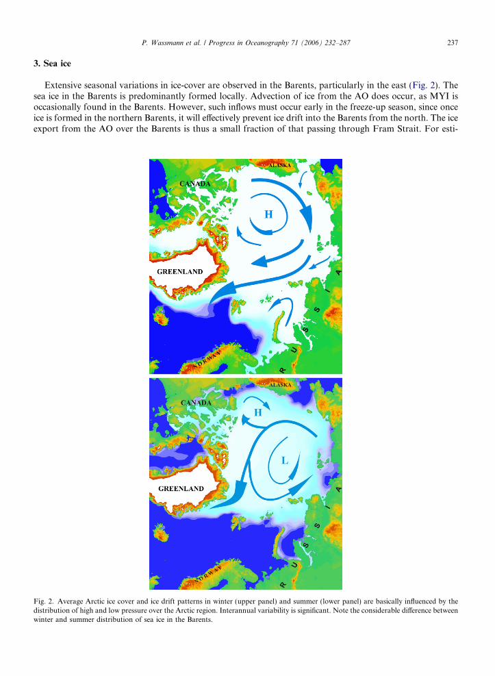
Extensive seasonal variations in ice-cover are observed in the Barents, particularly in the east (Fig. 2). Thesea ice in the Barents is predominantly formed locally. Advection of ice from the AO does occur, as MYI isoccasionally found in the Barents. However, such inflows must occur early in the freeze-up season, since onceice is formed in the northern Barents, it will effectively prevent ice drift into the Barents from the north. The iceexport from the AO over the Barents is thus a small fraction of that passing through Fram Strait. For esti-
Fig. 2. Average Arctic ice cover and ice drift patterns in winter (upper panel) and summer (lower panel) are basically influenced by thedistribution of high and low pressure over the Arctic region. Interannual variability is significant. Note the considerable difference betweenwinter and summer distribution of sea ice in the Barents.
238 P. Wassmann et al. / Progress in Oceanography 71 (2006) 232–287
mates of AO ice inflow into the northern Barents, see Section 7. The ice that drifts over AW melts rapidly byheating from below, creating a thin, low-salinity layer and a strong stratification above the AW in the centralBarents. This occurs throughout the year, and the strong stability ensures a rapid phytoplankton bloom in theupper layer once sufficient light is present (see Section 5).
Despite high interannual variability, the ice extent in the Barents has decreased by 60% over the last 200years (Vinje, 2001). The largest decrease in maximum ice extent took place before 1900 and between 1920and 1998. The decrease in the yearly maximum ice extent in April has been about 12%, while during the sameperiod the annual minimum ice cover in August has been reduced by 40%. Both the atmosphere and the oceanaffect the extent of the ice cover. The variability of the air temperature north of 62�N in the NA correlates wellwith the variability of the length of the solar (sun spot) cycle, indicating that the air temperature at these lat-itudes is mainly determined by solar radiation. This correlation has in recent years shown a tendency toweaken, which suggests a possible effect of the increased concentrations of greenhouse gases in the atmo-sphere, reducing the back radiation to space in winter (Vinje and Goosse, 2004). The extent of the ice coveralso depends on the temperature of the AW that enters the Barents, and a strong, inverse correlation is seenbetween the temperature at the Kola section and the ice extent (Loeng, 1991).
The importance of the wind field and the location of the storm tracks for the strength of the inflow of AWto the Barents and their relation to the relative strength of the Azores high pressure cell and the Icelandic lowpressure cell, the North Atlantic Oscillation (NAO), have been appreciated for some time (e.g. Loeng, 1992).However, it is during the last 10–15 years that NAO and its influence on the oceanic conditions in the NordicSeas have become foci for intense study. A positive NAO index leads to more northerly storm tracks andhigher air temperatures over the Nordic Seas. This results in an increase in both temperature and volumeof the Atlantic inflow to the Barents. A negative NAO index shifts the storm tracks southward, and the Polarhigh pressure cell is brought farther to the south leading to cold northerly and easterly winds over the Barents,thus to a reduced Atlantic inflow and increased ice formation (Fig. 2). The last 20 years have shown longerperiods of consistently positive NAO indices than previously. This may have acted to create the closer corre-lation between the air and the ocean temperatures mentioned above, making them act in synchrony to reduce(or increase) the extent of the ice cover (Vinje, 2001).
4. Nutrients and primary production
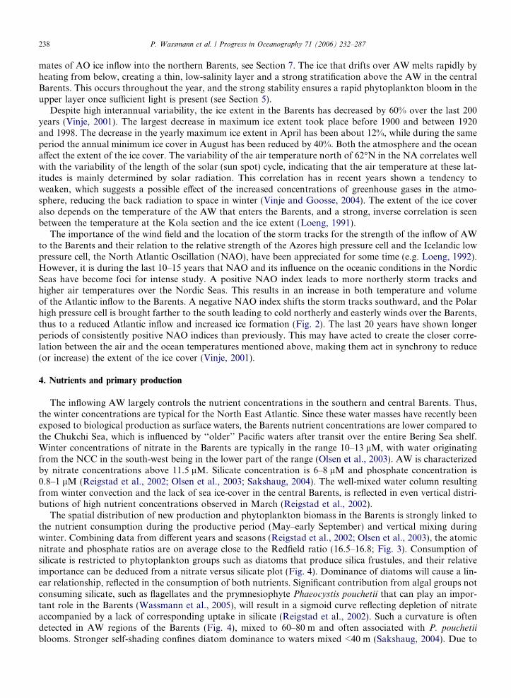
The inflowing AW largely controls the nutrient concentrations in the southern and central Barents. Thus,the winter concentrations are typical for the North East Atlantic. Since these water masses have recently beenexposed to biological production as surface waters, the Barents nutrient concentrations are lower compared tothe Chukchi Sea, which is influenced by ‘‘older’’ Pacific waters after transit over the entire Bering Sea shelf.Winter concentrations of nitrate in the Barents are typically in the range 10–13 lM, with water originatingfrom the NCC in the south-west being in the lower part of the range (Olsen et al., 2003). AW is characterizedby nitrate concentrations above 11.5 lM. Silicate concentration is 6–8 lM and phosphate concentration is0.8–1 lM (Reigstad et al., 2002; Olsen et al., 2003; Sakshaug, 2004). The well-mixed water column resultingfrom winter convection and the lack of sea ice-cover in the central Barents, is reflected in even vertical distri-butions of high nutrient concentrations observed in March (Reigstad et al., 2002).
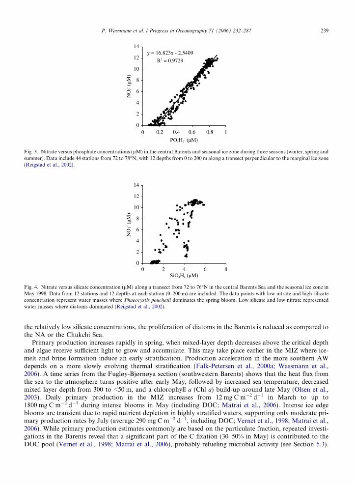
The spatial distribution of new production and phytoplankton biomass in the Barents is strongly linked tothe nutrient consumption during the productive period (May–early September) and vertical mixing duringwinter. Combining data from different years and seasons (Reigstad et al., 2002; Olsen et al., 2003), the atomicnitrate and phosphate ratios are on average close to the Redfield ratio (16.5–16.8; Fig. 3). Consumption ofsilicate is restricted to phytoplankton groups such as diatoms that produce silica frustules, and their relativeimportance can be deduced from a nitrate versus silicate plot (Fig. 4). Dominance of diatoms will cause a lin-ear relationship, reflected in the consumption of both nutrients. Significant contribution from algal groups notconsuming silicate, such as flagellates and the prymnesiophyte Phaeocystis pouchetii that can play an impor-tant role in the Barents (Wassmann et al., 2005), will result in a sigmoid curve reflecting depletion of nitrateaccompanied by a lack of corresponding uptake in silicate (Reigstad et al., 2002). Such a curvature is oftendetected in AW regions of the Barents (Fig. 4), mixed to 60–80 m and often associated with P. pouchetii
blooms. Stronger self-shading confines diatom dominance to waters mixed <40 m (Sakshaug, 2004). Due to
y = 16.823x - 2.5409
R2 = 0.9729
0
2
4
6
8
10
12
14
0 1
PO4H2- (µM)
NO
3- (µM
)0.2 0.4 0.6 0.8
Fig. 3. Nitrate versus phosphate concentrations (lM) in the central Barents and seasonal ice zone during three seasons (winter, spring andsummer). Data include 44 stations from 72 to 78�N, with 12 depths from 0 to 200 m along a transect perpendicular to the marginal ice zone(Reigstad et al., 2002).
0
2
4
6
8
10
12
14
0 2 4 6 8SiO4H4 (µM)
NO
3- (µM
)
Fig. 4. Nitrate versus silicate concentration (lM) along a transect from 72 to 76�N in the central Barents Sea and the seasonal ice zone inMay 1998. Data from 12 stations and 12 depths at each station (0–200 m) are included. The data points with low nitrate and high silicateconcentration represent water masses where Phaeocystis pouchetii dominates the spring bloom. Low silicate and low nitrate representedwater masses where diatoms dominated (Reigstad et al., 2002).
P. Wassmann et al. / Progress in Oceanography 71 (2006) 232–287 239
the relatively low silicate concentrations, the proliferation of diatoms in the Barents is reduced as compared tothe NA or the Chukchi Sea.
Primary production increases rapidly in spring, when mixed-layer depth decreases above the critical depthand algae receive sufficient light to grow and accumulate. This may take place earlier in the MIZ where ice-melt and brine formation induce an early stratification. Production acceleration in the more southern AWdepends on a more slowly evolving thermal stratification (Falk-Petersen et al., 2000a; Wassmann et al.,2006). A time series from the Fugløy-Bjørnøya section (southwestern Barents) shows that the heat flux fromthe sea to the atmosphere turns positive after early May, followed by increased sea temperature, decreasedmixed layer depth from 300 to <50 m, and a chlorophyll a (Chl a) build-up around late May (Olsen et al.,2003). Daily primary production in the MIZ increases from 12 mg C m�2 d�1 in March to up to1800 mg C m�2 d�1 during intense blooms in May (including DOC; Matrai et al., 2006). Intense ice edgeblooms are transient due to rapid nutrient depletion in highly stratified waters, supporting only moderate pri-mary production rates by July (average 290 mg C m�2 d�1, including DOC; Vernet et al., 1998; Matrai et al.,2006). While primary production estimates commonly are based on the particulate fraction, repeated investi-gations in the Barents reveal that a significant part of the C fixation (30–50% in May) is contributed to theDOC pool (Vernet et al., 1998; Matrai et al., 2006), probably refueling microbial activity (see Section 5.3).
240 P. Wassmann et al. / Progress in Oceanography 71 (2006) 232–287
Similar allocations have been shown in the North Water Polynya and are related to nutrient stress (Mei et al.,2003).
4.1. Ice and primary production
Light conditions under the ice vary with ice thickness and sediment load, and particularly snow cover ontop of the ice. The irradiance immediately below different types of ice and their algal layers in the Barents var-ies between 0.2% and 5% of the surface photosynthetically available radiation (Sakshaug et al., 1994). Ice algalcells are continuously shade adapted, although self-shading may cause light limitation of growth rates duringthe spring. Despite 24 h of daylight during May, the irradiance during hours of low sun is substantially less.Consequently, the dim phase production (6 h) is much lower than that during the rest of the day (18 h)(Hegseth, 1998). The growth rate for the ice algae in the Barents in May is about 0.2 cell div. d�1 (Johnsenand Hegseth, 1991). These differences in production need to be accounted for in calculations of the annualproduction for the northern Barents. The total ice algal production ranged between 0.16 and 52 mg C m�2 d�1
(100 days) and was 1.30 mg C m�2 for nights (60), giving a maximum annual production of 5.3 g C m�2 (Hegs-eth, 1998) for the ice-covered region of the Barents (Table 1). This is comparable to production estimates forsome other high Arctic areas (e.g. Horner and Schrader, 1982) but only half of what Legendre et al. (1992)estimated for the Arctic as a whole. The Barents estimate implies that ice algae comprise only about 6% ofthe total, average annual primary production in that area. However, the annual ice-related production isbetween 17% and 22% of the total primary production in the northern Barents, depending on whether the areanorth of Kvitøya is open water (Table 1). Thus, even in the perpetually ice-covered regions of the northernBarents pelagic primary production comprises the greatest source of energy.
4.2. Spatial and interannual variability in primary production
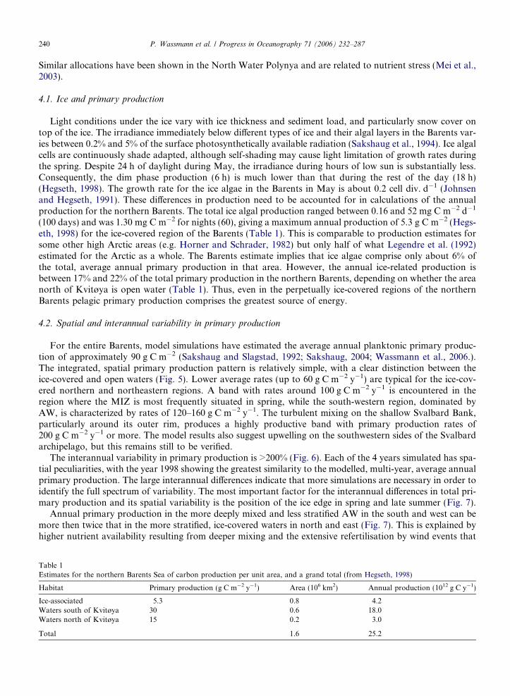
For the entire Barents, model simulations have estimated the average annual planktonic primary produc-tion of approximately 90 g C m�2 (Sakshaug and Slagstad, 1992; Sakshaug, 2004; Wassmann et al., 2006.).The integrated, spatial primary production pattern is relatively simple, with a clear distinction between theice-covered and open waters (Fig. 5). Lower average rates (up to 60 g C m�2 y�1) are typical for the ice-cov-ered northern and northeastern regions. A band with rates around 100 g C m�2 y�1 is encountered in theregion where the MIZ is most frequently situated in spring, while the south-western region, dominated byAW, is characterized by rates of 120–160 g C m�2 y�1. The turbulent mixing on the shallow Svalbard Bank,particularly around its outer rim, produces a highly productive band with primary production rates of200 g C m�2 y�1 or more. The model results also suggest upwelling on the southwestern sides of the Svalbardarchipelago, but this remains still to be verified.
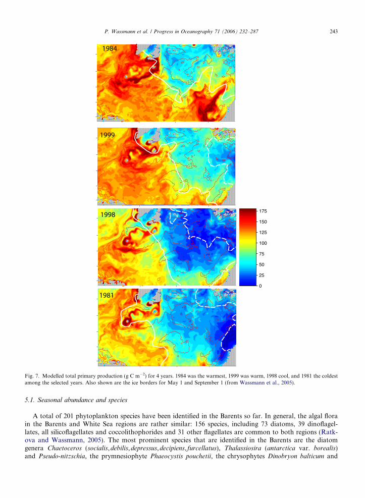
The interannual variability in primary production is >200% (Fig. 6). Each of the 4 years simulated has spa-tial peculiarities, with the year 1998 showing the greatest similarity to the modelled, multi-year, average annualprimary production. The large interannual differences indicate that more simulations are necessary in order toidentify the full spectrum of variability. The most important factor for the interannual differences in total pri-mary production and its spatial variability is the position of the ice edge in spring and late summer (Fig. 7).
Annual primary production in the more deeply mixed and less stratified AW in the south and west can bemore then twice that in the more stratified, ice-covered waters in north and east (Fig. 7). This is explained byhigher nutrient availability resulting from deeper mixing and the extensive refertilisation by wind events that
Table 1Estimates for the northern Barents Sea of carbon production per unit area, and a grand total (from Hegseth, 1998)
Habitat Primary production (g C m�2 y�1) Area (106 km2) Annual production (1012 g C y�1)
Ice-associated 5.3 0.8 4.2Waters south of Kvitøya 30 0.6 18.0Waters north of Kvitøya 15 0.2 3.0
Total 1.6 25.2
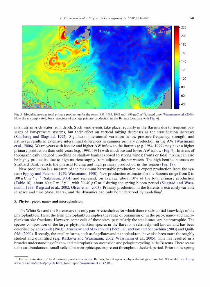
Fig. 5. Modelled average total primary production for the years 1981, 1984, 1998 and 1999 (g C m�2), based upon Wassmann et al. (2006).Note the uncomplicated, basic structure of average primary production in the Barents (compare with Fig. 6).
P. Wassmann et al. / Progress in Oceanography 71 (2006) 232–287 241
mix nutrient-rich water from depth. Such wind events take place regularly in the Barents due to frequent pas-sages of low-pressure systems, but their effect on vertical mixing decreases as the stratification increases(Sakshaug and Slagstad, 1992). Significant interannual variation in low-pressure frequency, strength, andpathways results in extensive interannual differences in summer primary production in the AW (Wassmannet al., 2006). Warm years with less ice and higher AW inflow to the Barents (e.g. 1984, 1999) may have a higherprimary production than cold years (e.g. 1998, 1981) with much ice and lower AW inflow (Fig. 7). In areas oftopographically induced upwelling or shallow banks exposed to strong winds; fronts or tidal mixing can alsobe highly productive due to high nutrient supply from adjacent deeper waters. The high benthic biomass onSvalbard Bank reflects the physical forcing and high primary production in this region (Fig. 19).
New production is a measure of the maximum harvestable production or export production from the sys-tem (Eppley and Peterson, 1979; Wassmann, 1990). New production estimates for the Barents range from 8 to100 g C m�2 y�1 (Sakshaug, 2004) and represent, on average, about 50% of the total primary production(Table 10): about 60 g C m�2 y�1, with 30–40 g C m�2 during the spring bloom period (Slagstad and Wass-mann, 1997; Reigstad et al., 2002; Olsen et al., 2003). Primary production in the Barents is extremely variablein space and time (days, years), and the dynamics can only be understood by modelling1.
5. Phyto-, pico-, nano- and microplankton
The White Sea and the Barents are the only pan-Arctic shelves for which there is substantial knowledge of thephytoplankton. Here, the term phytoplankton implies the range of organisms of in the pico-, nano- and micro-plankton size fractions. However, some cells of these sizes, particularly the small ones, are heterotrophic. Thespecies composition of the larger phytoplankton species in the Barents is relatively well known and has beendescribed by Zenkevich (1963), Druzhkov and Makarevich (1992), Kuznetsov and Schoschina (2003) and Quill-feldt (2000). Recently, the smaller forms, such as flagellates and nanoplankton, have also been more thoroughlystudied and quantified (e.g. Ratkova and Wassmann, 2002; Wassmann et al., 2005). This has resulted in abroader understanding of nano- and microplankton succession and pelagic recycling in the Barents. There seemsto be an abundance of small-celled, heterotrophic species present throughout the dark period. Prior to the spring
1 For an animation of total primary production in the Barents, based upon a physical–biological coupled 3D model, see http://www.nfh.uit.no/arctos/projects.html, based upon Wassmann et al. (2006).
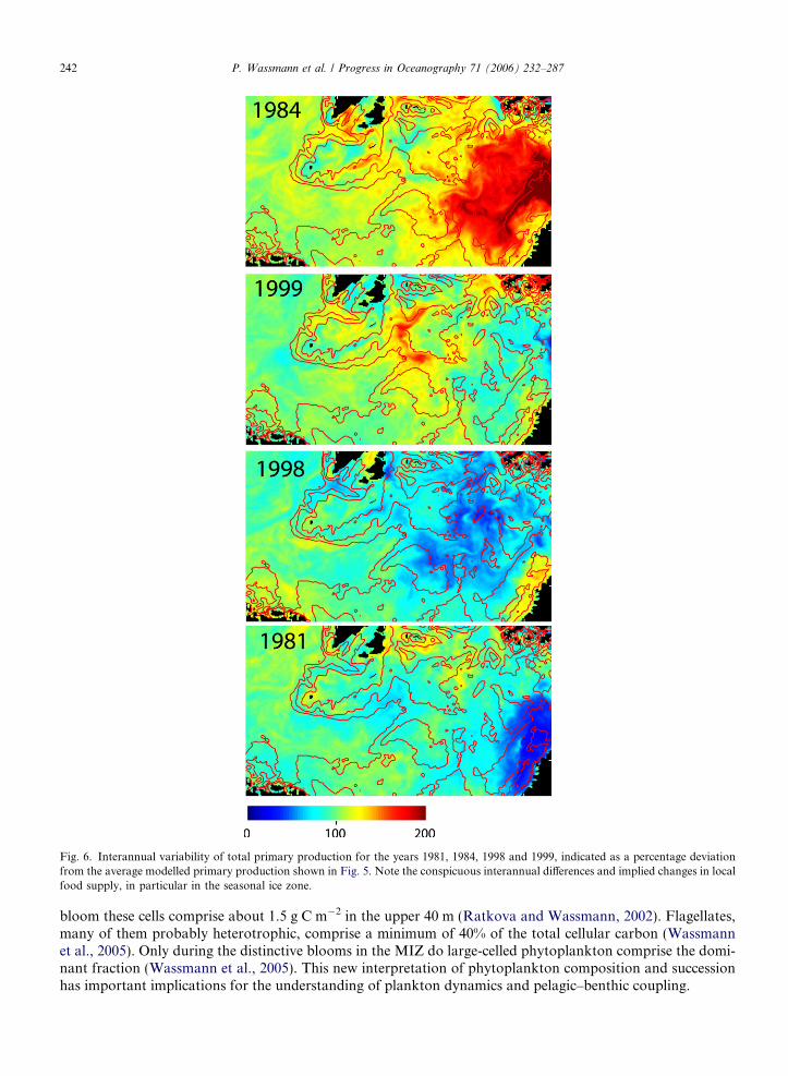
Fig. 6. Interannual variability of total primary production for the years 1981, 1984, 1998 and 1999, indicated as a percentage deviationfrom the average modelled primary production shown in Fig. 5. Note the conspicuous interannual differences and implied changes in localfood supply, in particular in the seasonal ice zone.
242 P. Wassmann et al. / Progress in Oceanography 71 (2006) 232–287
bloom these cells comprise about 1.5 g C m�2 in the upper 40 m (Ratkova and Wassmann, 2002). Flagellates,many of them probably heterotrophic, comprise a minimum of 40% of the total cellular carbon (Wassmannet al., 2005). Only during the distinctive blooms in the MIZ do large-celled phytoplankton comprise the domi-nant fraction (Wassmann et al., 2005). This new interpretation of phytoplankton composition and successionhas important implications for the understanding of plankton dynamics and pelagic–benthic coupling.
1984
1999
0
25
50
75
100
125
150
1751998
1981
Fig. 7. Modelled total primary production (g C m�2) for 4 years. 1984 was the warmest, 1999 was warm, 1998 cool, and 1981 the coldestamong the selected years. Also shown are the ice borders for May 1 and September 1 (from Wassmann et al., 2005).
P. Wassmann et al. / Progress in Oceanography 71 (2006) 232–287 243
5.1. Seasonal abundance and species
A total of 201 phytoplankton species have been identified in the Barents so far. In general, the algal florain the Barents and White Sea regions are rather similar: 156 species, including 73 diatoms, 39 dinoflagel-lates, all silicoflagellates and coccolithophorides and 31 other flagellates are common to both regions (Ratk-ova and Wassmann, 2005). The most prominent species that are identified in the Barents are the diatomgenera Chaetoceros (socialis,debilis,depressus,decipiens, furcellatus), Thalassiosira (antarctica var. borealis)and Pseudo-nitzschia, the prymnesiophyte Phaeocystis pouchetii, the chrysophytes Dinobryon balticum and
244 P. Wassmann et al. / Progress in Oceanography 71 (2006) 232–287
Ochromonas spp. and the dinoflagellates Diplopelta cf. parva, Diplosalis lenticula, Gymnodinium spp.,Gonyaulax digitale and Alexandrium tamarense. Most of the species are found both in the water columnand associated with sea ice. Fifty seem to be obligate to open water, e.g. the diatoms (Diatoma tenuis,Grammatophora arctica, Gyrosigma fasciola, Hantzschia sp., Chaetoceros borealis, Chaetoceros decipiens,Chaetoceros diadema, Coscinodiscus asteromphalus, Coscinodiscus centralis; the dinoflagellates Dinophysis
contracta, Gymnodinium arcticum, Heterocapsa spp., Katodinium sp., Prorocentrum micans, Protoperidinium
bipes, Protoperidinium pallidum, Protoperidinium pellucidum and a few other flagellates). For more completetaxonomic lists, see Jensen and Hansen (2000) and Ratkova and Wassmann (2002, 2005). Total pico-,nano- and microplankton biomass ranged between 4 and 14 g C m2 (in March and July, respectively).Besides the unidentified flagellates and monads, diatoms and prymnesiophytes (predominantly P. pouchetii)dominated.
0
20
40
60
80
100
0
50
100
150
200
Mar May Jun Jul
0
10
20
30
40
50
0
10
20
30
40
50
312
Cel
l 10
7 L-1
Cel
l 10
7 L-1
Cel
l 10
7 L-1
Cel
l 10
7 L-1
Diatoms
Phaeocystis pouchetii
Chrysophyceae
Choanoflagellidea
Unidentified flagellates
Unidentified monads
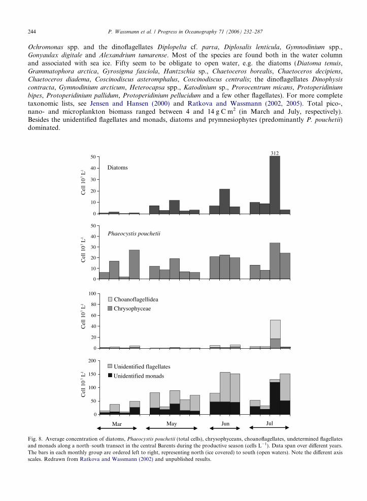
Fig. 8. Average concentration of diatoms, Phaeocystis pouchetii (total cells), chrysophyceans, choanoflagellates, undetermined flagellatesand monads along a north–south transect in the central Barents during the productive season (cells L�1). Data span over different years.The bars in each monthly group are ordered left to right, representing north (ice covered) to south (open waters). Note the different axisscales. Redrawn from Ratkova and Wassmann (2002) and unpublished results.
Table 2Average biomass of the main taxonomic groups observed in the 0–90 m layer (mg C m�2) along north–south gradients in the centralBarents Sea and MIZ
Season March 1998 May 1998 June/July 1999
Number of the stations 15 17 18
Diatoms 460 3380 3040Dinoflagellates 17 145 490Silicoflagellates + 180 6Coccolithophorides 6 6 10Prymnesiophytes 350 3530 3480Chrysomonades 100 250 1250Choanoflagellates 160 28 35Prasinophytes + � 5Cryptophytes 7 75 55Chlorophytes + + +Euglenophytes 4 7 3Zoomastigophores 1 + 11Unidentified flagellates and monads 2640 3600 4600Picophytoplankton 540 610 450Cyanobacteria � 90 55
Total 4285 11,900 13,490
+: <1 mg C m�2; �: not found. Recalculated from Ratkova and Wassmann (2002).
P. Wassmann et al. / Progress in Oceanography 71 (2006) 232–287 245
The abundance and concentration of the most prominent taxa are presented in Fig. 8 and Table 2.Phytoplankton succession in the Barents is difficult to outline, as time-series data from particular sitesor water masses do not exist. We have thus composed a phytoplankton succession in the spring to sum-mer season for different zones along a north–south gradient (ice-cover, MIZ, open water) for the years1998 and 1999 (Ratkova and Wassmann, 2002, and unpublished data). The abundance of diatoms islow in March, but increases steadily throughout the productive season (Fig. 8a). For the prymnesiophyteP. pouchetii, the patterns are different. The abundance (single cells) is already high in early spring and theseasonal variability is small. Blooms dominated by colonies are not so prominent and single cells usuallydominate in spring-early summer. Chrysophytes and choanoflagellates are not abundant during spring, butincrease in summer. Abundances of unidentified flagellates and monads are the highest of all algal groups,with a clear increasing trend through the productive season. A species succession is observed for the dia-toms from spring to summer in weakly stratified AW: from mainly small, single-celled Chaetoceros spp. toNitzschia spp.- and Thalassiosira spp.-dominated communities. Development of resting spores is commonfor Chaetoceros spp.
Below the ice, flagellates may be very abundant and comprise up to 98% of phytoplankton biomass. Theproportion of flagellates decreases with time to about 33% during the diatom bloom in the MIZ. Dinoflagel-lates are never abundant in late winter, but increase by mid-summer. A diatom bloom starts with the sea icespecies Fossula arctica, Fragilariopsis cylindrus, followed by F. oceanica. Later Thalassiosira spp. and P. pouch-
etii are found in ice-covered Atlantic and Arctic waters.Zooplankton can significantly influence the phytoplankton abundance, either by grazing on a certain size
category, species or the entire spectrum of cells, and top-down regulation has been assumed to be pivotal inthe northeastern North Atlantic (e.g. Wassmann et al., 1999b). For example, the abundance of P. pouchetiimay reflect grazing. Single cells of P. pouchetii seem to dominate over colonial cell biomass in the Barents,and during some years, while in some regions colonial cells seem rare (Wassmann et al., 2005). We speculatethat variable top-down regulation of P. pouchetii blooms possibly determines the ratio between single andcolonial cells, where grazing by mesozooplankton removes colonies and microzooplankton. As a consequence,the relative abundance of single cells increases. Overwintering and advection of larger mesozooplankton arewidespread in the Barents (Wassmann, 2001; Edvardsen et al., 2003), and grazing upon microzooplankton,large phytoplankton cells and colonies frequently results in accumulation of auto- and heterotrophic flagel-lates (Ratkova et al., 1999; Verity et al., 1999; Ratkova and Wassmann, 2002).
246 P. Wassmann et al. / Progress in Oceanography 71 (2006) 232–287
5.2. Bloom propagation and phytoplankton succession
The spring bloom starts in a band-like manner along the ice edge in late April and is particularly apparentin May, with concentrations of >250 mg Chl a m�2 (Fig. 9). The bloom is initiated by increased solar radia-tion, stratification induced by the ice-melt and abundant winter-accumulated nutrients. In the AW region, ver-tical mixing results in dilution of the growing phytoplankton, and the bloom peak is delayed. Theconcentrations usually are lower there compared to the MIZ. An ice-edge bloom accompanies the recedingedge northwards, but the bloom concentrations decrease northwards and over time (Figs. 9 and 10). Meltingsnow and sea ice allow large-scale primary production under the thinning ice-cover, sometimes at great dis-tance from the ice edge. The zooplankton community grazes upon phytoplankton, decreasing the phytoplank-ton stocks. Over the productive period, the band of the ice edge bloom develops into a ‘‘blooming plate’’ thatcovers most of the Barents (Fig. 10). At any time during the productive season a ‘‘spring-type’’ bloom will beencountered at the MIZ, according to Sakshaug and Skjoldal (1989), implying that during an expedition thatmoves from south to north in summer all stages of the plankton succession (summer to late winter) will bediscovered. Consequently, development over time (succession) can be encountered in space. However, theauthors original MIZ developmental concept, suggesting a steady, continuous and strong, northward-move-ment of a ‘‘spring-type’’ bloom, as illustrated by in the uppermost panels in Fig. 10, is only partly valid. Theice-edge bloom at the outskirts of the receding MIZ is not as steady and prominent like in late May (upperpanel in Fig. 10), but weakens over time and develops more and more into a weaker summer bloom with amore even intensity (lower panel, Fig. 10). We suggest that transects perpendicular to the MIZ do only toa certain extent represent time and succession. The MIZ bloom in the north in summer has a different qualitycompared to the one in May in the south. The MIZ bloom may also develop in the northern Barents due toearly sea ice melt and propagate southward (Falk-Petersen et al., 2000a).
The central Barents MIZ thus has a complex zonal structure in which the vernal bloom starts in the south-ern part of the MIZ. In a wave-like motion the vernal bloom proceeds both north (ice edge) and south (delayeddue to vertical mixing), as reflected in 2-D and 3-D biological–physical coupled models (Wassmann and Slags-tad, 1993; Slagstad and Wassmann, 1997; Wassmann et al., 2006). One part of the vernal bloom seeminglypropagates from the southern MIZ into the open AW, regulated by slowly decreasing vertical mixing. Thisbloom is wide and abundant as it covers the entire southern part of the central Barents (e.g. in June,Fig. 9). The other wave propagates steadily to the north as a more or less narrow band along with the recedingice-edge from mid-May onwards (combined effects of light penetration and stratification), as described bySakshaug and Skjoldal (1989). A minor wave propagates from the ice-free northern Barents towards the cen-tre. Light limitation in September–October brings the ice-edge bloom to an end (Hegseth, 1998), and usuallyChla concentrations are then <50 mg m�2 (Fig. 9).
5.3. The microbial food web: preliminary results and perspectives
Scattered investigations (e.g. Thingstad and Martinussen, 1991; Hansen et al., 1996; Hansen and Jensen,2000; Arashkevich et al., 2002; Verity et al., 2002; Wassmann et al., 2005) in the Barents indicate that smallplanktonic forms including microbes are as prevalent as in other biogeographic regions. Model work that hasnot been validated with data from the field suggests that microbial grazing is far greater than that of the largerCalanus species (Wassmann et al., 2006). Also, this model suggests that adult Calanus need to graze both onautotrophic and heterotrophic microplankton, as large-sized autotrophs may be scarce. State-of-the-art stud-ies of the microbial food web in the Barents are clearly lacking, but they are essential for a more balancedunderstanding of the pelagic ecosystem. At present, we cannot provide an adequate account of the microbialfood web, but we indicate some basic features in order to approximate its significance in the overall pelagicfood web.
Investigations close to the Barents entrance (Verity et al., 1999) and in its MIZ (Verity et al., 2002) sug-gest that often more than half of the dominating pico- and nano-plankton cell biomass is heterotrophic. Asmall fraction of the total bacterial cells (usually 108, max. 6 · 109 cells L�1) are dead, and a significant frac-tion (25–80%) of the total bacteria are dormant or expresses little activity (Howard-Jones et al., 2002; Stur-lusson, 2005). Bacterial production matched the likely extracellular primary production in May, and
Fig. 9. Modelled, integrated chlorophyll a concentrations (0–50 m, mg m�2) at various periods in the productive period in the Barents.Based upon Slagstad and McClimans (2005) and Wassmann et al. (2006). 1998 (left) and 1999 (right).
P. Wassmann et al. / Progress in Oceanography 71 (2006) 232–287 247
protozooplankton ingested up to 15–50% of the primary production during late spring (Hansen et al., 1996;Sturlusson, 2005). The protozoans were fully sufficient to feed the copepods, but so far grazing studies in theBarents have considered primarily phytoplankton. Other components of mesozooplankton diets in the
Fig. 10. Schematic development of the seasonal chlorophyll a concentration in the Barents (mg m�3). Along the panel tops, the positionand concentration of ice cover is depicted in blue. As the ice recedes northwards and gets thinner, the strength of the characteristic ice edgebloom diminishes with time and develops into a phytoplankton layer observable by September as a chlorophyll maximum in the south andas a subsurface bloom in the north. Note that minor marginal ice edge blooms may also develop in the opposite direction, i.e. north tosouth, in certain years.
248 P. Wassmann et al. / Progress in Oceanography 71 (2006) 232–287
Barents have so far not been specifically investigated. The microbial loop is obviously an important path-way by which carbon is channelled through the food web in the Barents. Cold-water ecosystems, such as theBarents, may share similarities with better-known, low-latitude regions where the microbial food web has aprominent role.
6. Zooplankton
Large populations of fish, sea birds and marine mammals migrate northwards in the Barents to feed on thelipid-rich zooplankton that can occur in large swarms. The high production and biomass of zooplankton aredue to: (1) high annual primary production and a pronounced phytoplankton spring bloom, in close associ-ation with the receding ice edge producing copious food for herbivorous zooplankton (e.g. Fig. 9); (2) advec-tion of zooplankton into the Barents from the Norwegian Sea with the NAC (e.g. Wassmann, 2001;Edvardsen et al., 2003); (3) advection of zooplankton from the AO with the EGC recirculating onto the wes-tern Svalbard shelf break; (4) transport of ice fauna from the AO into the Barents where organisms arereleased during the melting process (see Section 7.3), and (5) an efficient lipid-based energy flux (Jensenand Hansen, 2000; Falk-Petersen et al., 1990, 2000b).
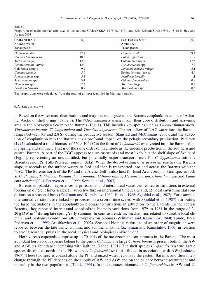
Table 3Proportion of main zooplankton taxa at the stations CABANERA I (75�N, 14�E), and Erik Eriksen Strait (79�N, 18�E) in July andAugust 2003
CABANERA I (%) Erik Eriksen Strait (%)Atlantic Water Arctic shelfTaxa/species Taxa/species
Oithona similis 27.1 Oithona similis 39.4Calanus finmarchicus 18.2 Calanus glacialis 21.2Metridia longa 12.2 Calanoida nauplii 17.5Echinodermata larvae 12.0 Pseudocalanus spp. 7.3Calanoida nauplii 9.2 Limacina helicina veliger 5.1Calanus glacialis 5.9 Echinodermata larvae 4.0Pseudocalanus spp. 5.4 Fritillaria borealis 1.1Microcalanus spp. 3.4 Calanus finmarchicus 0.9Oikopleura spp. 2.3 Metridia longa 0.6Fritillaria borealis 0.7 Microcalanus spp. 0.6
The proportions were calculated from the total of all taxa identified in Multinet samples.
P. Wassmann et al. / Progress in Oceanography 71 (2006) 232–287 249
6.1. Larger forms
Based on the water mass distributions and major current systems, the Barents zooplankton can be of Atlan-tic, Arctic or shelf origin (Table 3). The NAC transports species from their core distribution and spawningarea in the Norwegian Sea into the Barents (Fig. 1). This includes key species such as Calanus finmarchicus,Thysanoessa inermis, T. longicaudata and Themisto abyssorum. The net inflow of NAC water into the Barentsranges between 0.8 and 2.8 Sv during the productive season (Slagstad and McClimans, 2005), and the advec-tion of zooplankton into the Barents has a profound impact on the pelagic secondary production. Pedersen(1995) calculated a total biomass of 660 · 103 t C in the form of C. finmarchicus advected into the Barents dur-ing spring and summer. That is of the same order of magnitude as the endemic production in the southern andcentral Barents. A part of the EGC appears to turn eastwards and most likely hits the shelf slope of Svalbard(Fig. 1), representing an unquantified, but potentially major transport route for C. hyperboreus into theBarents region (S. Falk-Petersen, unpubl. data). When the deep-dwelling C. hyperboreus reaches the Barentsslope, it ascends to the surface waters to feed and then is transported into and across the Barents with theNAC. The Barents north of the PF and the Arctic shelf is also host for local Arctic zooplankton species suchas C. glacialis, T. libellula, Pseudocalanus minutus, Oithona similis, Mertensia ovum, Clione limacina and Lima-
cina helicina (Falk-Petersen et al., 1999; Søreide et al., 2003).Barents zooplankton experiences large seasonal and interannual variations related to variations in external
forcing on different times scales: (1) advective flux on interannual time scales and, (2) local environmental con-ditions on a seasonal basis (Zelikman and Kamshilov, 1960; Hassel, 1986; Skjoldal et al., 1987). For example,interannual variations are linked to processes on a several time scales, with Skjoldal et al. (1987) attributingthe large fluctuations in the zooplankton biomass to variations in advection to the Barents. In the centralBarents, they reported interannual zooplankton biomass variations from 1979 to 1984 in the range of 2–20 g DW m�2 during late spring/early summer. In contrast, endemic mechanisms related to variable local cli-matic and biological conditions affect zooplankton biomass (Zelikman and Kamshilov, 1960; Tande, 1991;Pedersen et al., 1995; Arashkevich et al., 2002). Seasonal biomass variations of an order of magnitude werereported between the late winter minima and summer maxima (Zelikman and Kamshilov, 1960) in relationto strong seasonal pulses in the local physical and biological environment.
Herbivorous copepods comprise up to 70–90% of the mesozooplankton biomass in the Barents. The mostabundant herbivorous species belong to the genus Calanus. The large C. hyperboreus is present both in the AWand ArW, its abundance increasing with latitude (Tande, 1991). The shelf species C. glacialis is a true Arcticspecies distributed north of the PF, whereas C. finmarchicus is distributed in association with AW (Jashnov,1967). These two species coexist along the PF and mixed water regions in the eastern Barents, and their inter-change through the PF depends on the supply of AW and ArW and on the balance between recruitment andmortality in the two populations (Tande, 1991). In mid-summer, biomass of C. finmarchicus in AW and C.
250 P. Wassmann et al. / Progress in Oceanography 71 (2006) 232–287
glacialis in ArW can reach 4.0 and 3.8 g DW m�2, respectively (Arashkevich et al., 2002). The biomass of C.
hyperboreus peaks at around 3 g DW m�2 at late summer (Tande, 1991).Calanus hyperboreus experiences a life cycle of several years. Its spawning period occurs prior to the spring
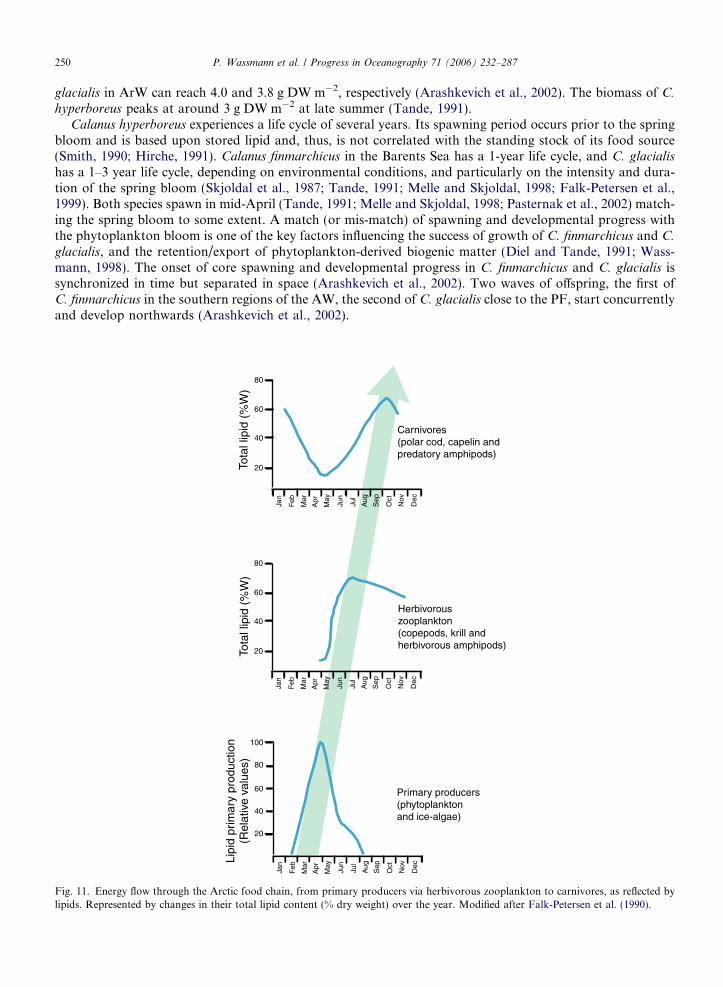
bloom and is based upon stored lipid and, thus, is not correlated with the standing stock of its food source(Smith, 1990; Hirche, 1991). Calanus finmarchicus in the Barents Sea has a 1-year life cycle, and C. glacialis
has a 1–3 year life cycle, depending on environmental conditions, and particularly on the intensity and dura-tion of the spring bloom (Skjoldal et al., 1987; Tande, 1991; Melle and Skjoldal, 1998; Falk-Petersen et al.,1999). Both species spawn in mid-April (Tande, 1991; Melle and Skjoldal, 1998; Pasternak et al., 2002) match-ing the spring bloom to some extent. A match (or mis-match) of spawning and developmental progress withthe phytoplankton bloom is one of the key factors influencing the success of growth of C. finmarchicus and C.
glacialis, and the retention/export of phytoplankton-derived biogenic matter (Diel and Tande, 1991; Wass-mann, 1998). The onset of core spawning and developmental progress in C. finmarchicus and C. glacialis issynchronized in time but separated in space (Arashkevich et al., 2002). Two waves of offspring, the first ofC. finmarchicus in the southern regions of the AW, the second of C. glacialis close to the PF, start concurrentlyand develop northwards (Arashkevich et al., 2002).
Jan
Feb
Mar
Apr
May
Oct
Nov
Aug
Sep
Jul
Jun
Dec
Jan
Feb
Mar
Apr
May
Oct
Nov
Aug
Sep
Jul
Jun
Dec
Jan
Feb
Mar
Apr
May
Oct
Nov
Aug
Sep
Jul
Jun
Dec
Carnivores(polar cod, capelin andpredatory amphipods)
Herbivorous zooplankton(copepods, krill andherbivorous amphipods)
Primary producers(phytoplanktonand ice-algae)
Tota
l lip
id (
%W
)Li
pid
prim
ary
prod
uctio
n(R
elat
ive
valu
es)
100
80
60
40
20
Tota
l lip
id (
%W
)
80
60
40
20
80
60
40
20
Fig. 11. Energy flow through the Arctic food chain, from primary producers via herbivorous zooplankton to carnivores, as reflected bylipids. Represented by changes in their total lipid content (% dry weight) over the year. Modified after Falk-Petersen et al. (1990).
P. Wassmann et al. / Progress in Oceanography 71 (2006) 232–287 251
The lipid-based energy flux through the food web, from algae to marine mammals (Fig. 11) is likely a keydeterminant of the productivity in the Barents environment. The organic compounds produced by photosyn-thesis are rapidly converted into large, specialized lipid (oil) stores by the herbivorous zooplankton (Lee, 1975;Sargent and Henderson, 1986; Falk-Petersen et al., 2006). The organic matter produced during the Barentsphytoplankton bloom in spring can in this way be transferred as high-energy fatty acids from phytoplanktonto top predators within a season via herbivorous zooplankton (Falk-Petersen et al., 1990).
6.2. Small forms
Small copepods (Pseudocalanus acuspes, P. minutus, Microcalanus pusillus, M. pygmaeus and O. similis)occur at high abundance in both Atlantic and Arctic domains (Hassel, 1986; Norrbin, 1991) (Table 3). Theirabundance varies with season and years and sometimes amounts to more than 50% of total mesozooplanktonnumbers (Hassel, 1986; Arashkevich et al., 2002). Young stages and nauplii of these copepods are too small tobe retained properly with standard-sized netting (e.g. 180 lm mesh size) and therefore their numbers can besignificantly underestimated. When collected with 90 lm mesh nets, the total number of small copepodsincreases over the productive period, peaking at around 2 · 106 ind. m�2 in AW and 2–3 · 106 ind. m�2 inArW in autumn (Norrbin, 1991). During the second half of summer when the older stages of Calanus spp.start entering diapause and descend to depths, small copepods and nauplii contribute about half of the zoo-plankton biomass in the upper 100 m layer (Arashkevich et al., 2002). Due to their numerical (and at timesbiomass) dominance and high specific metabolic rates, the frequently overlooked small species are importantin trophodynamic terms. Under post-bloom conditions, these species can participate in the trophic web inclose association with the microbial loop (see Section 5.3), where they may feed on heterotrophic protozoans.
7. Ice biota
The location of the ice edge during summer in the Barents (see Section 3) can vary by hundreds of kilometresfrom year to year (Maykut, 1985; Vinje and Kvambek, 1991; Gloersen et al., 1992; Johannessen et al., 2002).This has important implications for the distribution of ice flora and fauna and their contribution to the carbonbudget. The production of ice algae starts earlier than the plankton production and provides an early seasonfood source for the sympagic or ice-associated fauna and its predators, as well as feeding benthic organismsas the ice begins to melt in spring (Ambrose et al., 2005; McMahon et al., 2006; Renaud et al., 2006).
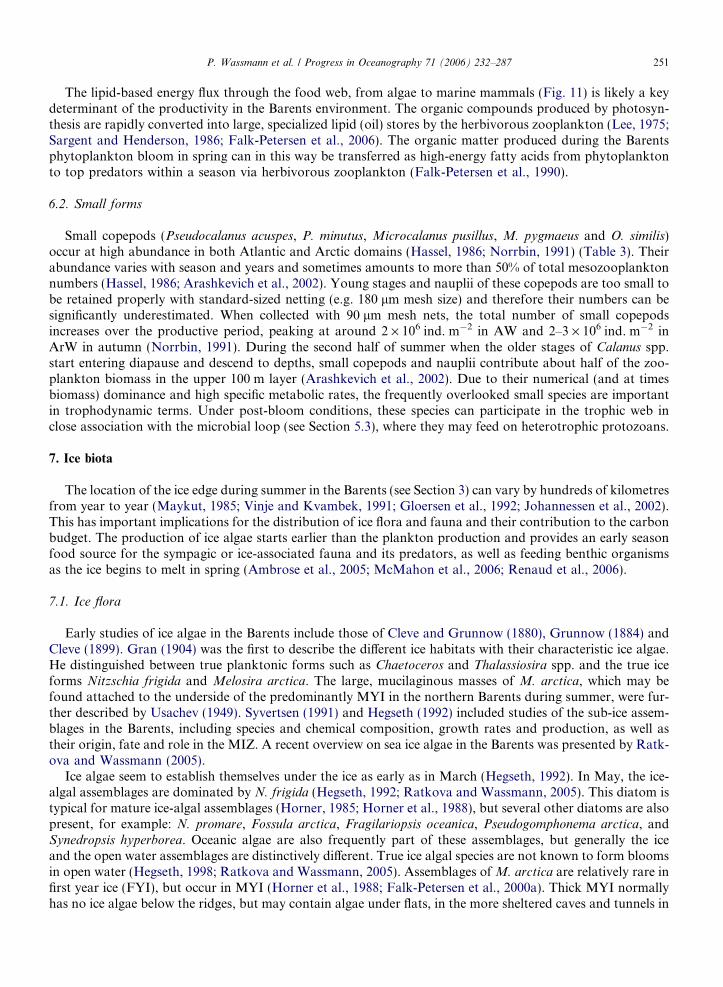
7.1. Ice flora
Early studies of ice algae in the Barents include those of Cleve and Grunnow (1880), Grunnow (1884) andCleve (1899). Gran (1904) was the first to describe the different ice habitats with their characteristic ice algae.He distinguished between true planktonic forms such as Chaetoceros and Thalassiosira spp. and the true iceforms Nitzschia frigida and Melosira arctica. The large, mucilaginous masses of M. arctica, which may befound attached to the underside of the predominantly MYI in the northern Barents during summer, were fur-ther described by Usachev (1949). Syvertsen (1991) and Hegseth (1992) included studies of the sub-ice assem-blages in the Barents, including species and chemical composition, growth rates and production, as well astheir origin, fate and role in the MIZ. A recent overview on sea ice algae in the Barents was presented by Ratk-ova and Wassmann (2005).
Ice algae seem to establish themselves under the ice as early as in March (Hegseth, 1992). In May, the ice-algal assemblages are dominated by N. frigida (Hegseth, 1992; Ratkova and Wassmann, 2005). This diatom istypical for mature ice-algal assemblages (Horner, 1985; Horner et al., 1988), but several other diatoms are alsopresent, for example: N. promare, Fossula arctica, Fragilariopsis oceanica, Pseudogomphonema arctica, andSynedropsis hyperborea. Oceanic algae are also frequently part of these assemblages, but generally the iceand the open water assemblages are distinctively different. True ice algal species are not known to form bloomsin open water (Hegseth, 1998; Ratkova and Wassmann, 2005). Assemblages of M. arctica are relatively rare infirst year ice (FYI), but occur in MYI (Horner et al., 1988; Falk-Petersen et al., 2000a). Thick MYI normallyhas no ice algae below the ridges, but may contain algae under flats, in the more sheltered caves and tunnels in
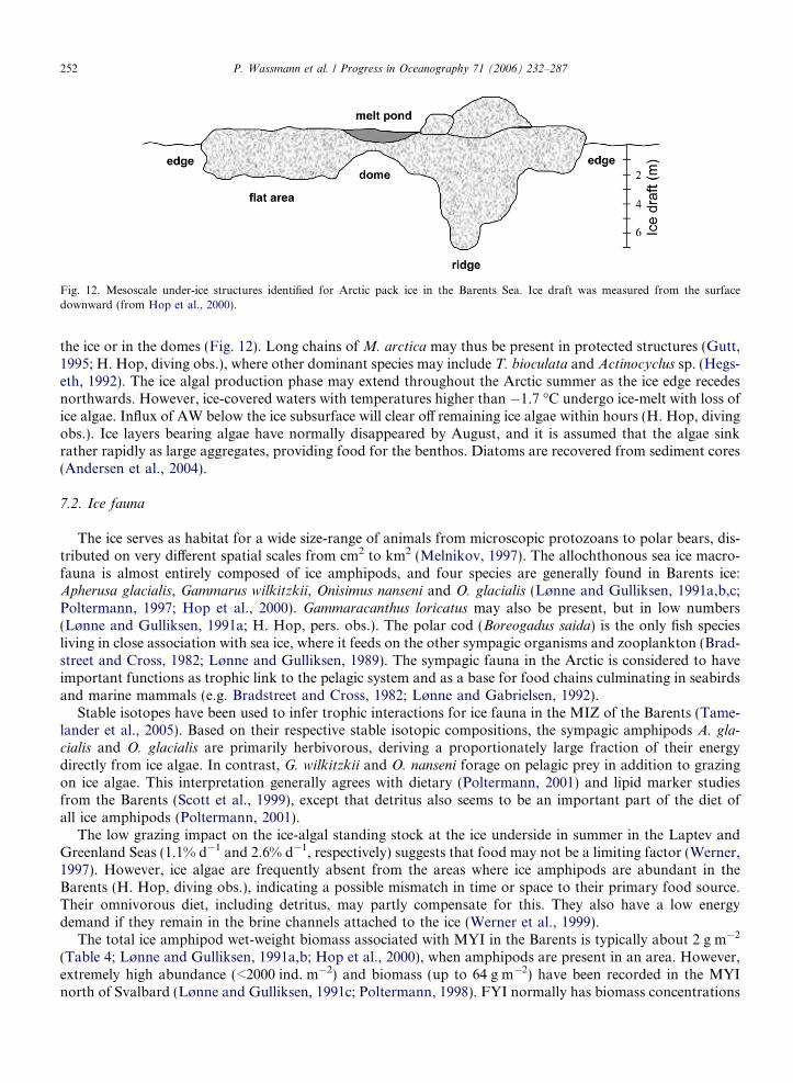
Fig. 12. Mesoscale under-ice structures identified for Arctic pack ice in the Barents Sea. Ice draft was measured from the surfacedownward (from Hop et al., 2000).
252 P. Wassmann et al. / Progress in Oceanography 71 (2006) 232–287
the ice or in the domes (Fig. 12). Long chains of M. arctica may thus be present in protected structures (Gutt,1995; H. Hop, diving obs.), where other dominant species may include T. bioculata and Actinocyclus sp. (Hegs-eth, 1992). The ice algal production phase may extend throughout the Arctic summer as the ice edge recedesnorthwards. However, ice-covered waters with temperatures higher than �1.7 �C undergo ice-melt with loss ofice algae. Influx of AW below the ice subsurface will clear off remaining ice algae within hours (H. Hop, divingobs.). Ice layers bearing algae have normally disappeared by August, and it is assumed that the algae sinkrather rapidly as large aggregates, providing food for the benthos. Diatoms are recovered from sediment cores(Andersen et al., 2004).
7.2. Ice fauna
The ice serves as habitat for a wide size-range of animals from microscopic protozoans to polar bears, dis-tributed on very different spatial scales from cm2 to km2 (Melnikov, 1997). The allochthonous sea ice macro-fauna is almost entirely composed of ice amphipods, and four species are generally found in Barents ice:Apherusa glacialis, Gammarus wilkitzkii, Onisimus nanseni and O. glacialis (Lønne and Gulliksen, 1991a,b,c;Poltermann, 1997; Hop et al., 2000). Gammaracanthus loricatus may also be present, but in low numbers(Lønne and Gulliksen, 1991a; H. Hop, pers. obs.). The polar cod (Boreogadus saida) is the only fish speciesliving in close association with sea ice, where it feeds on the other sympagic organisms and zooplankton (Brad-street and Cross, 1982; Lønne and Gulliksen, 1989). The sympagic fauna in the Arctic is considered to haveimportant functions as trophic link to the pelagic system and as a base for food chains culminating in seabirdsand marine mammals (e.g. Bradstreet and Cross, 1982; Lønne and Gabrielsen, 1992).
Stable isotopes have been used to infer trophic interactions for ice fauna in the MIZ of the Barents (Tame-lander et al., 2005). Based on their respective stable isotopic compositions, the sympagic amphipods A. gla-
cialis and O. glacialis are primarily herbivorous, deriving a proportionately large fraction of their energydirectly from ice algae. In contrast, G. wilkitzkii and O. nanseni forage on pelagic prey in addition to grazingon ice algae. This interpretation generally agrees with dietary (Poltermann, 2001) and lipid marker studiesfrom the Barents (Scott et al., 1999), except that detritus also seems to be an important part of the diet ofall ice amphipods (Poltermann, 2001).
The low grazing impact on the ice-algal standing stock at the ice underside in summer in the Laptev andGreenland Seas (1.1% d�1 and 2.6% d�1, respectively) suggests that food may not be a limiting factor (Werner,1997). However, ice algae are frequently absent from the areas where ice amphipods are abundant in theBarents (H. Hop, diving obs.), indicating a possible mismatch in time or space to their primary food source.Their omnivorous diet, including detritus, may partly compensate for this. They also have a low energydemand if they remain in the brine channels attached to the ice (Werner et al., 1999).
The total ice amphipod wet-weight biomass associated with MYI in the Barents is typically about 2 g m�2
(Table 4; Lønne and Gulliksen, 1991a,b; Hop et al., 2000), when amphipods are present in an area. However,extremely high abundance (<2000 ind. m�2) and biomass (up to 64 g m�2) have been recorded in the MYInorth of Svalbard (Lønne and Gulliksen, 1991c; Poltermann, 1998). FYI normally has biomass concentrations
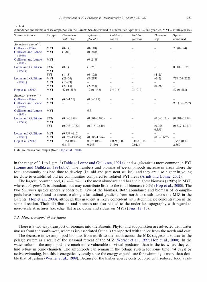
Table 4Abundance and biomass of ice amphipods in the Barents Sea determined in different ice types (FYI = first year ice, MYI = multi-year ice)
Source reference Icetype Gammarus
wilkitzkii
Apherusa
glacialis
Onisimus
nanseni
Onisimus
glacialis
Onisimus
spp.Speciescombined
Abundance (no m�2)
Gulliksen (1984) MYI (0–14) (0–118) – – – 20 (0–124)Gulliksen and Lønne
(1989)MYI (–200) (0–2488) – – – –
Gulliksen and Lønne(1991)
MYI (0–2488) – – – –
Lønne and Gulliksen(1991a)
FYI/MYI
(0–1) (1–25) – – – 0.001–0.179
FYI (1–18) (6–102) – – (4–25)Lønne and Gulliksen
(1991c)MYI (21–54) (8–2196) – – (0–2) 728 (54–2223)MYI (13–89) – – – – –MYI (2–113) (2–263) – – (0–26) –
Hop et al. (2000) MYI 47 (0–517) 12 (0–142) 0.4(0–6) 0.1(0–2) – 59 (0–518)
Biomass (g ww m�2)
Gulliksen (1984) MYI (0.0–1.26) (0.0–0.81) – – – –Gulliksen and Lønne
(1989)MYI – – – – – 9.6 (1.6–25.2)
Gulliksen and Lønne(1991)
MYI – 6.7 – – – –
Lønne and Gulliksen(1991a)
FYI/MYI
(0.0–0.179) (0.001–0.073) – – (0.0–0.121) (0.001–0.179)
FYI (0.043–0.762) (0.016–0.540) – – (0.056–0.355)
(0.339–1.381)
Lønne and Gulliksen(1991c)
MYI (0.954 –816) – – – – –MYI (0.025–13.857) (0.003–1.384) – – (0.0–0.667) –
Hop et al. (2000) MYI 1.854 (0.0–6.417)
0.073 (0.0–0.243)
0.029 (0.0–0.139)
0.002 (0.0–0.013)
– 1.958 (0.0–2.860)
Data are means and ranges (from Hop et al., 2000).
P. Wassmann et al. / Progress in Oceanography 71 (2006) 232–287 253
in the range of 0.1 to 1 g m�2 (Table 4; Lønne and Gulliksen, 1991a), and A. glacialis is more common in FYI(Lønne and Gulliksen, 1991a,b,c). The numbers and biomass of ice-amphipods increase in areas where thetotal community has had time to develop (i.e. old and persistent sea ice), and they are also higher in youngice close to established old ice communities compared to isolated FYI areas (Arndt and Lønne, 2002).
The largest ice-amphipod, G. wilkitzkii, is the most abundant and has the highest biomass (>90%) in MYI,whereas A. glacialis is abundant, but may contribute little to the total biomass (<4%) (Hop et al., 2000). Thetwo Onisimus species generally contribute <2% of the biomass. Both abundance and biomass of ice-amphi-pods have been found to decrease along a latitudinal gradient from north to south across the MIZ in theBarents (Hop et al., 2000), although this gradient is likely coincident with declining ice concentration in thesame direction. Their distribution and biomass are also related to the under-ice topography with regard tomeso-scale structures (i.e. edge, flat area, dome and ridges on MYI) (Figs. 12, 13).
7.3. Mass transport of ice fauna
There is a two-way transport of biomass into the Barents. Phyto- and zooplankton are advected with watermasses from the south-west, whereas ice-associated fauna is transported with the ice from the north and east.
The decrease in ice-amphipod biomass from north to the south across the MIZ suggests a source to thepelagic system as a result of the seasonal retreat of the MIZ (Werner et al., 1999; Hop et al., 2000). In thewater column, the amphipods are much more vulnerable to visual predators than in the ice where they canfind refuge in brine channels. The amphipods can remain in the pelagic system for some time (>4 days) byactive swimming, but this is energetically costly since the energy expenditure for swimming is more than dou-ble that of resting (Werner et al., 1999). Because of the higher energy costs coupled with reduced food avail-
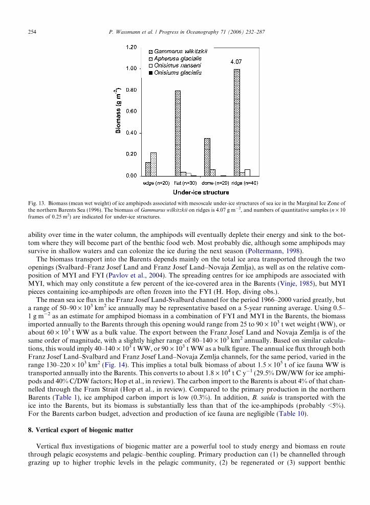
Fig. 13. Biomass (mean wet weight) of ice amphipods associated with mesoscale under-ice structures of sea ice in the Marginal Ice Zone ofthe northern Barents Sea (1996). The biomass of Gammarus wilkitzkii on ridges is 4.07 g m�2, and numbers of quantitative samples (n · 10frames of 0.25 m2) are indicated for under-ice structures.
254 P. Wassmann et al. / Progress in Oceanography 71 (2006) 232–287
ability over time in the water column, the amphipods will eventually deplete their energy and sink to the bot-tom where they will become part of the benthic food web. Most probably die, although some amphipods maysurvive in shallow waters and can colonize the ice during the next season (Poltermann, 1998).
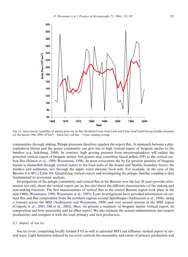
The biomass transport into the Barents depends mainly on the total ice area transported through the twoopenings (Svalbard–Franz Josef Land and Franz Josef Land–Novaja Zemlja), as well as on the relative com-position of MYI and FYI (Pavlov et al., 2004). The spreading centres for ice amphipods are associated withMYI, which may only constitute a few percent of the ice-covered area in the Barents (Vinje, 1985), but MYIpieces containing ice-amphipods are often frozen into the FYI (H. Hop, diving obs.).
The mean sea ice flux in the Franz Josef Land-Svalbard channel for the period 1966–2000 varied greatly, buta range of 50–90 · 103 km2 ice annually may be representative based on a 5-year running average. Using 0.5–1 g m�2 as an estimate for amphipod biomass in a combination of FYI and MYI in the Barents, the biomassimported annually to the Barents through this opening would range from 25 to 90 · 103 t wet weight (WW), orabout 60 · 103 t WW as a bulk value. The export between the Franz Josef Land and Novaja Zemlja is of thesame order of magnitude, with a slightly higher range of 80–140 · 103 km2 annually. Based on similar calcula-tions, this would imply 40–140 · 103 t WW, or 90 · 103 t WW as a bulk figure. The annual ice flux through bothFranz Josef Land–Svalbard and Franz Josef Land–Novaja Zemlja channels, for the same period, varied in therange 130–220 · 103 km2 (Fig. 14). This implies a total bulk biomass of about 1.5 · 105 t of ice fauna WW istransported annually into the Barents. This converts to about 1.8 · 104 t C y�1 (29.5% DW/WW for ice amphi-pods and 40% C/DW factors; Hop et al., in review). The carbon import to the Barents is about 4% of that chan-nelled through the Fram Strait (Hop et al., in review). Compared to the primary production in the northernBarents (Table 1), ice amphipod carbon import is low (0.3%). In addition, B. saida is transported with theice into the Barents, but its biomass is substantially less than that of the ice-amphipods (probably <5%).For the Barents carbon budget, advection and production of ice fauna are negligible (Table 10).
8. Vertical export of biogenic matter
Vertical flux investigations of biogenic matter are a powerful tool to study energy and biomass en routethrough pelagic ecosystems and pelagic–benthic coupling. Primary production can (1) be channelled throughgrazing up to higher trophic levels in the pelagic community, (2) be regenerated or (3) support benthic
320
300
280
260
240
220
200
180
160
140
120
100
80
60
1965 1970 1975 1980
Year
Are
a F
lux
(103
km2 )
1985 1990 1995 2000
Fig. 14. Inter-annual variability of annual mean sea ice flux (Svalbard-Franz Josef Land and Franz Josef Land-Novaja Zemlja channels)for the period 1966–2000 (103km2) – black line; red line – 5-year running average.
P. Wassmann et al. / Progress in Oceanography 71 (2006) 232–287 255
communities through sinking. Pelagic processes therefore regulate the export flux. A mismatch between a phy-toplankton bloom and the grazer community can give rise to high vertical export of biogenic matter to thebenthos (e.g. Sakshaug, 2004). In contrast, high grazing pressure from mesozooplankton will reduce thepotential vertical export of biogenic matter, but grazers may contribute faecal pellets (FP) to the vertical car-bon flux (Peinert et al., 1989; Wassmann, 1998). In most ecosystems the by far greatest quantity of biogenicmatter is channelled through vertical export to the food webs of the deeper and benthic boundary layers, thebenthos and sediments, not through the upper water platonic food web. For example, in the case of theBarents it is 80% (Table 10). Quantifying vertical export and investigating the pelagic–benthic coupling is thusfundamental to ecosystem analysis.
Investigations of the pelagic community and vertical flux in the Barents over the last 20 years provide infor-mation not only about the vertical export per se, but also about the different characteristics of the sinking andnon-sinking fractions. The first measurements of vertical flux in the central Barents region took place in themid-1980s (Wassmann, 1989; Wassmann et al., 1993). Later investigations have provided information on ver-tical flux and flux composition from the northern regions around Spitsbergen (Andreassen et al., 1996), alonga transect across the MIZ (Andreassen and Wassmann, 1998) and over several seasons in the MIZ region(Coppola et al., 2002; Olli et al., 2002). Here, we present a summary of biogenic matter vertical export, itscomposition and how seasonality and ice affect export. We also estimate the annual sedimentation rate (exportproduction) and compare it with the total primary and new production.
8.1. Impact of sea ice
Sea ice cover, comprising locally formed FYI as well as advected MYI can influence vertical export in sev-eral ways. Light limitation induced by ice-cover controls the seasonality and extent of primary production and
256 P. Wassmann et al. / Progress in Oceanography 71 (2006) 232–287
therefore vertical export. In seasonally ice-covered waters, the presence of ice with snow cover shortens theproductive season in the waters below compared to ice-free waters. The halocline resulting from ice-melt limitsnew production by creating a strong barrier for nutrient supply from depth, contrasting with the weaker ther-mocline developing in ice-free waters (Wassmann et al., 2006). Sedimentation rates in the partially ice-coveredparts of the central Barents are up to an order of magnitude higher than in the quasi-permanently ice coveredareas north of Spitsbergen (consolidated ice-cover). In July, sedimentation rates at 90 m depth ranged from100 to 200 mg C m�2 d�1 along a transect from 72 to 78�N, with lowest export at the ice-covered station inthe north and highest in the deeper, mixed, ice-free PF region (Olli et al., 2002).
Ice contributes to the export of organic matter by ice algae, especially mucilaginous masses of M. arctica
that are occasionally present under MYI and released during melting. Sedimentation of ice algae can be dif-ficult to trace as pelagic species might be frozen into the ice and released. Recent measurements of verticalexport immediately below the ice of the MIZ (using sub-ice sediment traps) indicate low export in areas whereice melting is pronounced. Only in regions with dense ice and early bloom conditions vertical export below theice and adjacent euphotic zone are in the same range (M. Reigstad, unpubl. data). Low export from the ice isrecorded from regions with pronounced ice melting. Observations of fluffy green algal material at the seafloorin the MIZ (M. Carroll, pers. comm.; McMinn and Hegseth, 2004) and evidence from stable isotope tracers(Tamelander et al., 2005) indicate, however, that ice algae can be an important input to the benthos, probablyreflecting detachment of algal mats and aggregate formation from the dense phytoplankton blooms. Theserather patchy and episodic events are difficult to resolve using short-term sediment traps.
Ice can also contribute directly to the vertical flux through ice rafted material such as sediments and detritus(e.g. Andreassen et al., 1996). The carbon export north of Spitsbergen ranged from 20 to 80 mg POC m�2 d�1
at 100 m depth containing high inorganic components and C/N ratios >26. This suggests terrestrial input,most likely of ‘‘dirty ice’’ from the Laptev Sea riding the Transpolar Drift.
8.2. Seasonality of vertical export
Seasonality in the Barents is not only related to the time of the year, but also to the continuously changingice conditions that affect primary and export production locally (Falk-Petersen et al., 2000a; Olli et al., 2002).Sedimentation rates measured in March (25–60 mg C m�2 d�1, at 90 m depth) are assumed to be representa-tive for the winter season. No nutrient drawdown was detectable in the water column, and the Chl a was neg-ligible (Olli et al., 2002; Reigstad et al., 2002). During the spring bloom period in May, the sedimentation ratesincreased more than 10 times at 90 m, ranging from 350 to 750 mg C m�2 d�1. The high vertical export of car-bon during the spring bloom points to the inability of grazers to cope with the high production, which leaves alarge fraction for export to benthic communities. Andreassen and Wassmann (1998) estimated high daily lossrates of Chl a of 4–18% in May. These high loss rates also coincide with high production of extra-cellular car-bon and mucilaginous matter, indicating that aggregation could be an important export mechanism.
During the summer season, the vertical export of carbon declined to 100–200 mg C m�2 d�1. This reflectsthe development of a more diverse and complex pelagic food web that retains suspended biomass and nutri-ents more efficiently (Olli et al., 2002). Few measurements exist from the autumn period, but Wassmann (1989)indicates sedimentation rates comparable to the lower range of those encountered in July data(100 mg C m�2 d�1, at 60 m in open water).
8.3. Vertical flux attenuation and composition
A strong vertical component in the carbon sedimentation exists in the upper 200 m, in particular in the twi-light zone, the lowest part of the euphotic and upper layer of the aphotic zone (Wassmann et al., 2003). Sed-iment trap measurements with high vertical resolution reveal how settling material changes with depth(Fig. 15). In winter (March) no vertical flux attenuation was discovered for POC (Fig. 15, left). Most ofthe settling POC could not be identified by microscopy, and this detritus did not appear to be exposed toany significant grazing or degradation during its descent. The scenario in spring (May) is radically different.High new production and suspended biomass result in high sedimentation rates, >1000 mg C m�2 d�1 justbelow the upper mixed layer, followed by a strong decline in the POC export (Fig. 15, centre left and right).
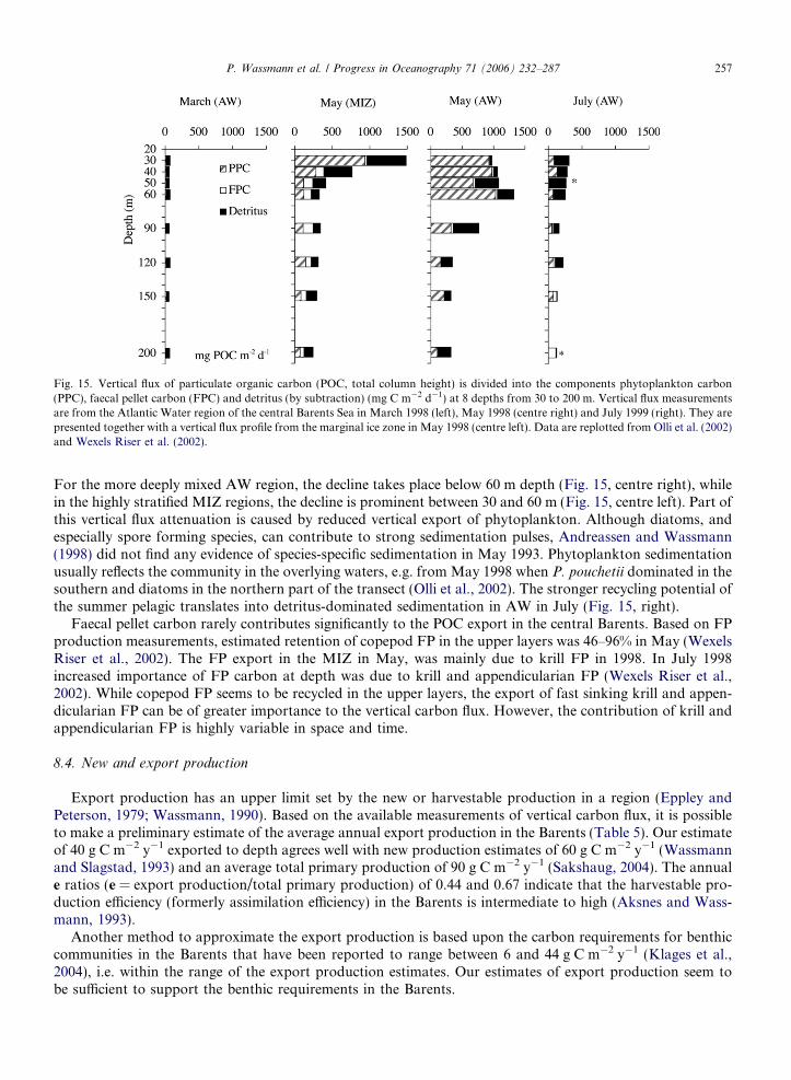
Fig. 15. Vertical flux of particulate organic carbon (POC, total column height) is divided into the components phytoplankton carbon(PPC), faecal pellet carbon (FPC) and detritus (by subtraction) (mg C m�2 d�1) at 8 depths from 30 to 200 m. Vertical flux measurementsare from the Atlantic Water region of the central Barents Sea in March 1998 (left), May 1998 (centre right) and July 1999 (right). They arepresented together with a vertical flux profile from the marginal ice zone in May 1998 (centre left). Data are replotted from Olli et al. (2002)and Wexels Riser et al. (2002).
P. Wassmann et al. / Progress in Oceanography 71 (2006) 232–287 257
For the more deeply mixed AW region, the decline takes place below 60 m depth (Fig. 15, centre right), whilein the highly stratified MIZ regions, the decline is prominent between 30 and 60 m (Fig. 15, centre left). Part ofthis vertical flux attenuation is caused by reduced vertical export of phytoplankton. Although diatoms, andespecially spore forming species, can contribute to strong sedimentation pulses, Andreassen and Wassmann(1998) did not find any evidence of species-specific sedimentation in May 1993. Phytoplankton sedimentationusually reflects the community in the overlying waters, e.g. from May 1998 when P. pouchetii dominated in thesouthern and diatoms in the northern part of the transect (Olli et al., 2002). The stronger recycling potential ofthe summer pelagic translates into detritus-dominated sedimentation in AW in July (Fig. 15, right).
Faecal pellet carbon rarely contributes significantly to the POC export in the central Barents. Based on FPproduction measurements, estimated retention of copepod FP in the upper layers was 46–96% in May (WexelsRiser et al., 2002). The FP export in the MIZ in May, was mainly due to krill FP in 1998. In July 1998increased importance of FP carbon at depth was due to krill and appendicularian FP (Wexels Riser et al.,2002). While copepod FP seems to be recycled in the upper layers, the export of fast sinking krill and appen-dicularian FP can be of greater importance to the vertical carbon flux. However, the contribution of krill andappendicularian FP is highly variable in space and time.
8.4. New and export production
Export production has an upper limit set by the new or harvestable production in a region (Eppley andPeterson, 1979; Wassmann, 1990). Based on the available measurements of vertical carbon flux, it is possibleto make a preliminary estimate of the average annual export production in the Barents (Table 5). Our estimateof 40 g C m�2 y�1 exported to depth agrees well with new production estimates of 60 g C m�2 y�1 (Wassmannand Slagstad, 1993) and an average total primary production of 90 g C m�2 y�1 (Sakshaug, 2004). The annuale ratios (e = export production/total primary production) of 0.44 and 0.67 indicate that the harvestable pro-duction efficiency (formerly assimilation efficiency) in the Barents is intermediate to high (Aksnes and Wass-mann, 1993).
Another method to approximate the export production is based upon the carbon requirements for benthiccommunities in the Barents that have been reported to range between 6 and 44 g C m�2 y�1 (Klages et al.,2004), i.e. within the range of the export production estimates. Our estimates of export production seem tobe sufficient to support the benthic requirements in the Barents.
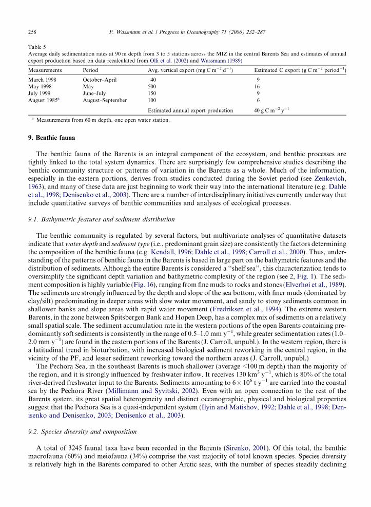
Table 5Average daily sedimentation rates at 90 m depth from 3 to 5 stations across the MIZ in the central Barents Sea and estimates of annualexport production based on data recalculated from Olli et al. (2002) and Wassmann (1989)
Measurements Period Avg. vertical export (mg C m�2 d�1) Estimated C export (g C m�2 period�1)
March 1998 October–April 40 9May 1998 May 500 16July 1999 June–July 150 9August 1985a August–September 100 6
Estimated annual export production 40 g C m�2 y�1
a Measurements from 60 m depth, one open water station.
258 P. Wassmann et al. / Progress in Oceanography 71 (2006) 232–287
9. Benthic fauna
The benthic fauna of the Barents is an integral component of the ecosystem, and benthic processes aretightly linked to the total system dynamics. There are surprisingly few comprehensive studies describing thebenthic community structure or patterns of variation in the Barents as a whole. Much of the information,especially in the eastern portions, derives from studies conducted during the Soviet period (see Zenkevich,1963), and many of these data are just beginning to work their way into the international literature (e.g. Dahleet al., 1998; Denisenko et al., 2003). There are a number of interdisciplinary initiatives currently underway thatinclude quantitative surveys of benthic communities and analyses of ecological processes.
9.1. Bathymetric features and sediment distribution
The benthic community is regulated by several factors, but multivariate analyses of quantitative datasetsindicate that water depth and sediment type (i.e., predominant grain size) are consistently the factors determiningthe composition of the benthic fauna (e.g. Kendall, 1996; Dahle et al., 1998; Carroll et al., 2000). Thus, under-standing of the patterns of benthic fauna in the Barents is based in large part on the bathymetric features and thedistribution of sediments. Although the entire Barents is considered a ‘‘shelf sea’’, this characterization tends tooversimplify the significant depth variation and bathymetric complexity of the region (see 2, Fig. 1). The sedi-ment composition is highly variable (Fig. 16), ranging from fine muds to rocks and stones (Elverhøi et al., 1989).The sediments are strongly influenced by the depth and slope of the sea bottom, with finer muds (dominated byclay/silt) predominating in deeper areas with slow water movement, and sandy to stony sediments common inshallower banks and slope areas with rapid water movement (Fredriksen et al., 1994). The extreme westernBarents, in the zone between Spitsbergen Bank and Hopen Deep, has a complex mix of sediments on a relativelysmall spatial scale. The sediment accumulation rate in the western portions of the open Barents containing pre-dominantly soft sediments is consistently in the range of 0.5–1.0 mm y�1, while greater sedimentation rates (1.0–2.0 mm y�1) are found in the eastern portions of the Barents (J. Carroll, unpubl.). In the western region, there isa latitudinal trend in bioturbation, with increased biological sediment reworking in the central region, in thevicinity of the PF, and lesser sediment reworking toward the northern areas (J. Carroll, unpubl.)
The Pechora Sea, in the southeast Barents is much shallower (average <100 m depth) than the majority ofthe region, and it is strongly influenced by freshwater inflow. It receives 130 km3 y�1, which is 80% of the totalriver-derived freshwater input to the Barents. Sediments amounting to 6 · 106 t y�1 are carried into the coastalsea by the Pechora River (Millimann and Syvitski, 2002). Even with an open connection to the rest of theBarents system, its great spatial heterogeneity and distinct oceanographic, physical and biological propertiessuggest that the Pechora Sea is a quasi-independent system (Ilyin and Matishov, 1992; Dahle et al., 1998; Den-isenko and Denisenko, 2003; Denisenko et al., 2003).
9.2. Species diversity and composition
A total of 3245 faunal taxa have been recorded in the Barents (Sirenko, 2001). Of this total, the benthicmacrofauna (60%) and meiofauna (34%) comprise the vast majority of total known species. Species diversityis relatively high in the Barents compared to other Arctic seas, with the number of species steadily declining
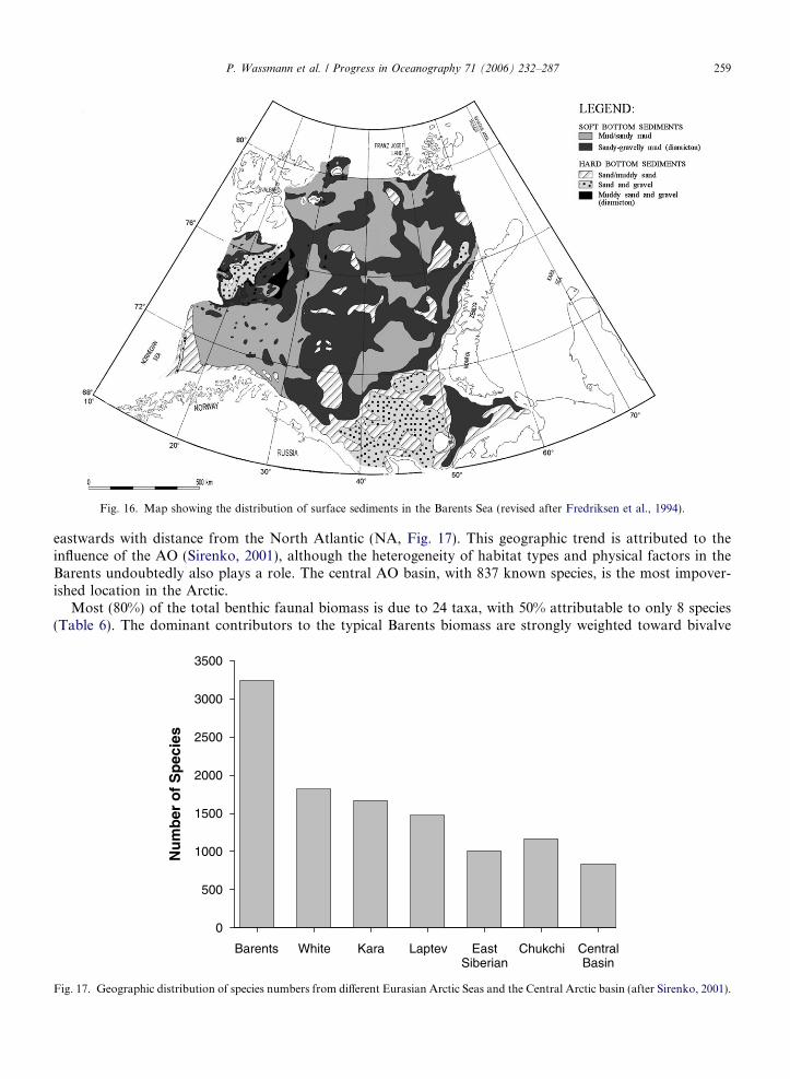
Fig. 16. Map showing the distribution of surface sediments in the Barents Sea (revised after Fredriksen et al., 1994).
P. Wassmann et al. / Progress in Oceanography 71 (2006) 232–287 259
eastwards with distance from the North Atlantic (NA, Fig. 17). This geographic trend is attributed to theinfluence of the AO (Sirenko, 2001), although the heterogeneity of habitat types and physical factors in theBarents undoubtedly also plays a role. The central AO basin, with 837 known species, is the most impover-ished location in the Arctic.
Most (80%) of the total benthic faunal biomass is due to 24 taxa, with 50% attributable to only 8 species(Table 6). The dominant contributors to the typical Barents biomass are strongly weighted toward bivalve
Nu
mb
er o
f S
pec
ies
0
500
1000
1500
2000
2500
3000
3500
Barents White Kara Laptev EastSiberian
Chukchi CentralBasin
Fig. 17. Geographic distribution of species numbers from different Eurasian Arctic Seas and the Central Arctic basin (after Sirenko, 2001).
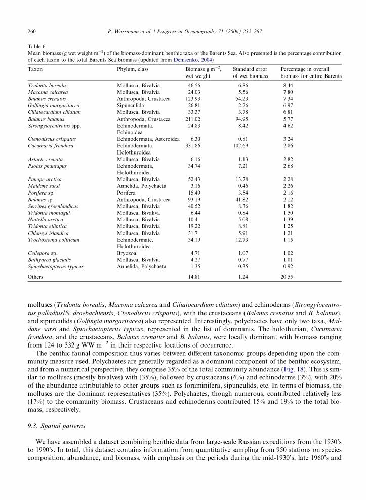
Table 6Mean biomass (g wet weight m�2) of the biomass-dominant benthic taxa of the Barents Sea. Also presented is the percentage contributionof each taxon to the total Barents Sea biomass (updated from Denisenko, 2004)
Taxon Phylum, class Biomass g m�2,wet weight
Standard errorof wet biomass
Percentage in overallbiomass for entire Barents
Tridonta borealis Mollusca, Bivalvia 46.56 6.86 8.44Macoma calcarea Mollusca, Bivalvia 24.03 5.56 7.80Balanus crenatus Arthropoda, Crustacea 123.93 54.23 7.34Golfingia margaritacea Sipunculida 26.81 2.26 6.97Ciliatocardium ciliatum Mollusca, Bivalvia 33.37 3.78 6.81Balanus balanus Arthropoda, Crustacea 211.02 94.95 5.77Strongylocentrotus spp. Echinodermata,
Echinoidea24.83 8.42 4.62
Ctenodiscus crispatus Echinodermata, Asteroidea 6.30 0.81 3.24Cucumaria frondosa Echinodermata,
Holothuroidea331.86 102.69 2.86
Astarte crenata Mollusca, Bivalvia 6.16 1.13 2.82Psolus phantapus Echinodermata,
Holothuroidea34.74 7.21 2.68
Panope arctica Mollusca, Bivalvia 52.43 13.78 2.28Maldane sarsi Annelida, Polychaeta 3.16 0.46 2.26Porifera sp. Porifera 15.49 3.54 2.16Balanus sp. Arthropoda, Crustacea 93.19 41.82 2.12Serripes groenlandicus Mollusca, Bivalvia 40.52 8.36 1.82Tridonta montagui Mollusca, Bivaliva 6.44 0.84 1.50Hiatella arctica Mollusca, Bivalvia 10.4 5.08 1.39Tridonta elliptica Mollusca, Bivalvia 19.22 8.81 1.25Chlamys islandica Mollusca, Bivalvia 31.7 5.91 1.21Trochostoma ooliticum Echinodermate,
Holothuroidea34.19 12.73 1.15
Cellepora sp. Bryozoa 4.71 1.07 1.02Bathyarca glacialis Mollusca, Bivalvia 4.27 0.77 1.01Spiochaetopterus typicus Annelida, Polychaeta 1.35 0.35 0.92
Others 14.81 1.24 20.55
260 P. Wassmann et al. / Progress in Oceanography 71 (2006) 232–287
molluscs (Tridonta borealis, Macoma calcarea and Ciliatocardium ciliatum) and echinoderms (Strongylocentro-
tus palladius/S. droebachiensis, Ctenodiscus crispatus), with the crustaceans (Balanus crenatus and B. balanus),and sipunculids (Golfingia margaritacea) also represented. Interestingly, polychaetes have only two taxa, Mal-
dane sarsi and Spiochaetopterus typicus, represented in the list of dominants. The holothurian, Cucumariafrondosa, and the crustaceans, Balanus crenatus and B. balanus, were locally dominant with biomass rangingfrom 124 to 332 g WW m�2 in their respective locations of occurrence.
The benthic faunal composition thus varies between different taxonomic groups depending upon the com-munity measure used. Polychaetes are generally regarded as a dominant component of the benthic ecosystem,and from a numerical perspective, they comprise 35% of the total community abundance (Fig. 18). This is sim-ilar to molluscs (mostly bivalves) with (35%), followed by crustaceans (6%) and echinoderms (3%), with 20%of the abundance attributable to other groups such as foraminifera, sipunculids, etc. In terms of biomass, themolluscs are the dominant representatives (35%). Polychaetes, though numerous, contributed relatively less(17%) to the community biomass. Crustaceans and echinoderms contributed 15% and 19% to the total bio-mass, respectively.
9.3. Spatial patterns
We have assembled a dataset combining benthic data from large-scale Russian expeditions from the 1930’sto 1990’s. In total, this dataset contains information from quantitative sampling from 950 stations on speciescomposition, abundance, and biomass, with emphasis on the periods during the mid-1930’s, late 1960’s and
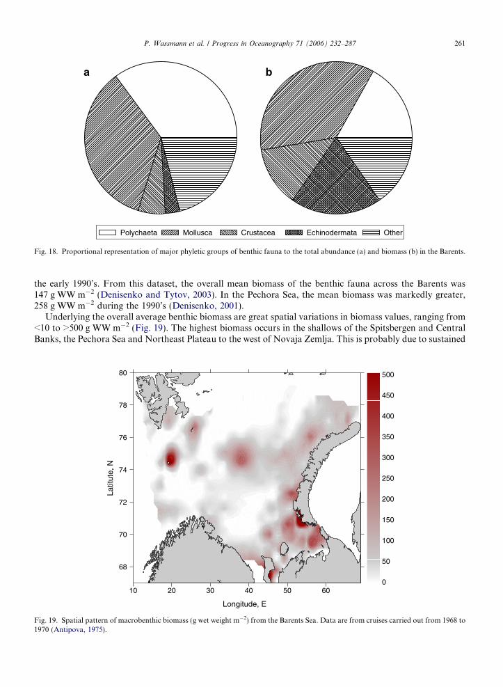
Polychaeta Mollusca Crustacea Echinodermata Other
Fig. 18. Proportional representation of major phyletic groups of benthic fauna to the total abundance (a) and biomass (b) in the Barents.
P. Wassmann et al. / Progress in Oceanography 71 (2006) 232–287 261
the early 1990’s. From this dataset, the overall mean biomass of the benthic fauna across the Barents was147 g WW m�2 (Denisenko and Tytov, 2003). In the Pechora Sea, the mean biomass was markedly greater,258 g WW m�2 during the 1990’s (Denisenko, 2001).
Underlying the overall average benthic biomass are great spatial variations in biomass values, ranging from<10 to >500 g WW m�2 (Fig. 19). The highest biomass occurs in the shallows of the Spitsbergen and CentralBanks, the Pechora Sea and Northeast Plateau to the west of Novaja Zemlja. This is probably due to sustained
10 20 30 40 50 60
Longitude, E
68
70
72
74
76
78
80
Latit
ute,
N
0
50
100
150
200
250
300
350
400
450
500
Fig. 19. Spatial pattern of macrobenthic biomass (g wet weight m�2) from the Barents Sea. Data are from cruises carried out from 1968 to1970 (Antipova, 1975).
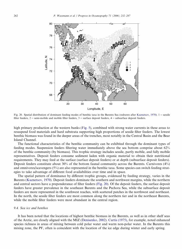
20 30 40 50 60
Longitude, E
68
70
72
74
76
78
80
Latit
ude,
N
1 to 2 2 to 3 3 to 4 4 to 5
Fig. 20. Spatial distribution of dominant feeding modes of benthic taxa in the Barents Sea (redrawn after Kuznetsov, 1970). 1 = sessilefilter feeders, 2 = semi-mobile and mobile filter feeders, 3 = surface deposit feeders, 4 = subsurface deposit feeders.
262 P. Wassmann et al. / Progress in Oceanography 71 (2006) 232–287
high primary production at the western banks (Fig. 5), combined with strong water currents in these areas toresuspend food materials and hard substrata supporting high proportions of sessile filter feeders. The lowestbenthic biomass was found in the deeper areas of the trenches, most notably in the Central Basin and the BearIsland Channel.
The functional characteristics of the benthic community can be exhibited through the dominant types offeeding modes. Suspension feeders filtering water immediately above the sea bottom comprise about 62%of the benthic community (by biomass). This trophic strategy includes sessile, partly mobile, and fully mobilerepresentatives. Deposit feeders consume sediment laden with organic material to obtain their nutritionalrequirements. They may feed at the surface (surface deposit feeders) or at depth (subsurface deposit feeders).Deposit feeders constitute about 30% of the bottom faunal community across the Barents. Carnivores (4%)and omnivores/scavengers (5%) are also represented in the benthic taxa. Some species can switch feeding strat-egies to take advantage of different food availabilities over time and in space.
The spatial pattern of dominance by different trophic groups, evidenced by feeding strategy, varies in theBarents (Kuznetsov, 1970). Deposit feeders dominate the southern and northwest margins, while the northernand central sectors have a preponderance of filter feeders (Fig. 20). Of the deposit feeders, the surface depositfeeders have greater prevalence in the southeast Barents and the Pechora Sea, while the subsurface depositfeeders are more represented in the southwest reaches, with scattered patches in the northwest and northeast.In the north, the sessile filter feeders are most common along the northern tier and in the northeast Barents,while the mobile filter feeders were most abundant in the central region.
9.4. Sea ice and benthos
It has been noted that the locations of highest benthic biomass in the Barents, as well as in other shelf seasof the Arctic, are closely aligned with the MIZ (Denisenko, 2002). Curtis (1975), for example, noted enhancedspecies richness in areas of mixing between cold polar water and warm non-polar water. In the Barents thismixing zone, the PF, often is coincident with the location of the ice edge during winter and early spring.
P. Wassmann et al. / Progress in Oceanography 71 (2006) 232–287 263
In the Barents, depth nullifies benthic microalgae or macrophytes as a contributing food source for all butthe shallowest fringe areas. Thus, benthic fauna are completely reliant on surface ocean processes for food.Increased benthic biomass, through greater availability of organic material, results from enhanced primaryproduction in the surface and/or more efficient delivery of surface production to the sea bottom.
The conditions necessary for enhanced primary production are provided by three elements: (1) the MIZphytoplankton bloom, (2) primary production under the pycnocline, and (3) contribution by ice algae. Nutri-ent enhancement may result from turbulent mixing of nutrient-rich AW into the upper stratified Arctic layeralong (but not north of) the PF (Slagstad and Stokke, 1984). This results in prolonged bloom conditions at thePF (often associated with the ice edge) compared to other areas. Ice algae, typically diatoms, which grow rap-idly under the ice as soon as the light conditions permit and up to the time of intensive ice melting, commonlycolonize the MIZ (see Section 7.1). While ice algae may provide an overall minor source of primary produc-tion to the system as a whole, the timing ice algal inputs to the systems is important. The peak in ice algalbiomass generally precedes the pelagic bloom by 1–2 months (Strass and Nothig, 1996), and the releaseand sinking of ice algae during the period of ice melting may provide an early-season food source to the ben-thos (Stabeno and Overland, 2001).
The fate of the primary production in the system largely depends upon the amount of time the cells spend inthe water column and the grazing pressure (see Section 8.3). Diatom cells sink faster than smaller flagellatecells. Large chains of cells, as are common in ice-edge bloom conditions, sink faster yet, often avoiding inges-tion or degradation on the way to the sea bottom (Smetacek, 1985). The MIZ bloom is not caused by partic-ularly high annual primary production rates (Figs. 5 and 7), but by stratification and light. In concert thisresults in rapid phytoplankton development and a high concentration of suspended biomass in the stratifiedupper 20 m (>18 mg chl a m�3, Wassmann et al., 1999a; Matrai et al., 2006). The intensified pelagic–benthiccoupling in the MIZ is caused by the high suspended concentration (m�3), intense zooplankton grazing (FP)and the resulting increase of aggregation potential. Most vertical flux scenarios encountered so far in the MIZof the Barents suggest high vertical export, but also significant vertical flux attenuation (Fig. 15).
9.5. Temporal patterns
The characteristics of benthic fauna, many of which are long-lived and sessile, make them ideal integratorsand indicators of environmental changes. Changes in species distribution and abundance related to tempera-ture have been demonstrated for a number of individual species (Zenkevich, 1963; Galkin, 1998), while var-iable interannual growth of individual populations of bivalves has been linked to oscillatory climatic patterns(Ambrose et al., 2006). Thus, community changes through time can potentially provide an understanding ofthe linkage between the environment and the marine ecosystem (e.g. Beuchel et al., 2006). Such an analysisbenefits greatly from regularly repeated, quantitative sampling of benthos at representative locations, whichunfortunately has been the exception rather than the rule in Arctic areas.
This limitation has inhibited attempts to examine rigorously changes in communities through time. None-theless, there are enough data from some specific time periods to get an idea of decadal variations in benthiccommunities. In particular datasets from 1924–1932 and 1968–1970 seem extensive enough to examine com-munity changes for the entire Barents soft-bottom habitat (Antipova, 1975; Galkin, 1998; Denisenko, 2001).The biomass distribution clearly shows differences between the two time periods (Fig. 21). Although the rel-ative locations of high biomass generally correspond between them, the overall magnitude of biomass wasreduced by 60% in the late 1960’s compared to the late 1920’s. Regular sea temperature measurements con-ducted along the Kola Transect since the beginning of the 20th century indicate that the late 1960’s was a par-ticularly cold period, with a water temperature 0.5 �C below the 20th century average of 3.9 �C, including oneparticularly cold year in 1966 with mean annual water temperature of 2.8 �C. While Antipova (1975) attributesthe decrease in benthic biomass in the 1960’s to the cold-water temperatures, Denisenko (2001) suggests amore complex relationship. In an analysis focusing only on the Kola Transect for which there are more phys-ical and biological data than for elsewhere in the Barents, he suggests that the variations, not only in the 1960’sbut also in several other decades of the 20th century, are more strongly related to direct anthropogenic dis-turbance, in the form of intensity of bottom trawling, than to temperature fluctuations. Using a 4-year lag-function, Denisenko (2001) found an astounding correlation of �0.98 between trawling intensity and benthic
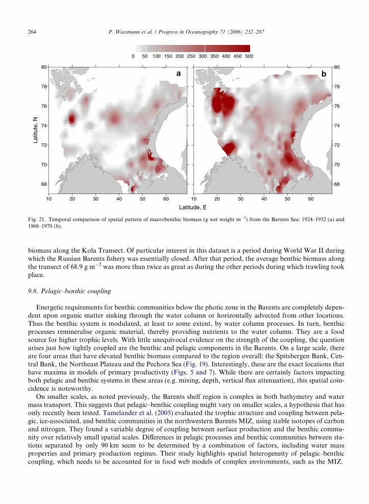
10 20 30 40 50 60
68
70
72
74
76
78
80
Latit
ute,
N
10 20 30 40 50 60
68
70
72
74
76
78
80
0 50 100 150 200 250 300 350 400 450 500
Latitude, E
a b
Fig. 21. Temporal comparison of spatial pattern of macrobenthic biomass (g wet weight m�2) from the Barents Sea: 1924–1932 (a) and1968–1970 (b).
264 P. Wassmann et al. / Progress in Oceanography 71 (2006) 232–287
biomass along the Kola Transect. Of particular interest in this dataset is a period during World War II duringwhich the Russian Barents fishery was essentially closed. After that period, the average benthic biomass alongthe transect of 68.9 g m�2 was more than twice as great as during the other periods during which trawling tookplace.
9.6. Pelagic–benthic coupling
Energetic requirements for benthic communities below the photic zone in the Barents are completely depen-dent upon organic matter sinking through the water column or horizontally advected from other locations.Thus the benthic system is modulated, at least to some extent, by water column processes. In turn, benthicprocesses remineralise organic material, thereby providing nutrients to the water column. They are a foodsource for higher trophic levels. With little unequivocal evidence on the strength of the coupling, the questionarises just how tightly coupled are the benthic and pelagic components in the Barents. On a large scale, thereare four areas that have elevated benthic biomass compared to the region overall: the Spitsbergen Bank, Cen-tral Bank, the Northeast Plateau and the Pechora Sea (Fig. 19). Interestingly, these are the exact locations thathave maxima in models of primary productivity (Figs. 5 and 7). While there are certainly factors impactingboth pelagic and benthic systems in these areas (e.g. mixing, depth, vertical flux attenuation), this spatial coin-cidence is noteworthy.
On smaller scales, as noted previously, the Barents shelf region is complex in both bathymetry and watermass transport. This suggests that pelagic–benthic coupling might vary on smaller scales, a hypothesis that hasonly recently been tested. Tamelander et al. (2005) evaluated the trophic structure and coupling between pela-gic, ice-associated, and benthic communities in the northwestern Barents MIZ, using stable isotopes of carbonand nitrogen. They found a variable degree of coupling between surface production and the benthic commu-nity over relatively small spatial scales. Differences in pelagic processes and benthic communities between sta-tions separated by only 90 km seem to be determined by a combination of factors, including water massproperties and primary production regimes. Their study highlights spatial heterogeneity of pelagic–benthiccoupling, which needs to be accounted for in food web models of complex environments, such as the MIZ.
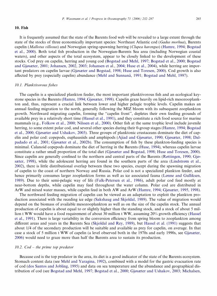
P. Wassmann et al. / Progress in Oceanography 71 (2006) 232–287 265
10. Fish
It is frequently assumed that the state of the Barents food web will be revealed to a large extent through thestate of the stocks of three economically important species: Northeast Atlantic cod (Gadus morhua), Barentscapelin (Mallotus villosus) and Norwegian spring-spawning herring (Clupea harengus) (Hamre, 1994; Bogstadet al., 2000). Both total fish production in the Norwegian-Barents Sea area (including Norwegian coastalwaters), and other aspects of the total ecosystem, appear to be closely linked to the development of thesestocks. Cod prey on capelin, herring and young cod (Bogstad and Mehl, 1997; Bogstad et al., 2000; Bogstadand Gjøsæter, 2001; Johansen, 2002, 2003; Johansen et al., 2004; Huse et al., 2004), while herring are impor-tant predators on capelin larvae (Gjøsæter and Bogstad, 1998; Huse and Toresen, 2000). Cod growth is alsoaffected by prey (especially capelin) abundance (Mehl and Sunnana, 1991; Bogstad and Mehl, 1997).
10.1. Planktivorous fishes
The capelin is a specialized plankton feeder, the most important planktivorous fish and an ecological key-stone species in the Barents (Hamre, 1994; Gjøsæter, 1998). Capelin graze heavily on lipid-rich mesozooplank-ton and, thus, represent a crucial link between lower and higher pelagic trophic levels. Capelin makes anannual feeding migration to the north, generally following the MIZ bloom with its subsequent zooplanktongrowth. Northward migrating capelin, forming the ‘‘capelin front’’, depletes their own feeding grounds ofavailable prey in a relatively short time (Hassel et al., 1991), and they constitute a rich food source for marinemammals (e.g., Folkow et al., 2000; Nilssen et al., 2000). Other fish at the same trophic level include juvenileherring, to some extent polar cod, and several other species during their 0-group stages (Hamre, 1994; Bogstadet al., 2000; Gjøsæter and Ushakov, 2003). Three groups of planktonic crustaceans dominate the diet of cap-elin and polar cod: copepods, euphausiids and amphipods (Ajiad and Gjøsæter, 1990; Gjøsæter, 1998; Dal-padado et al., 2001; Gjøsæter et al., 2002b). The consumption of fish by these plankton-feeding species isminimal. Calanoid copepods dominate the diet of herring in the Barents (Huse, 1994), whereas capelin larvaeconstitute a rather small proportion of the total diet (Gjøsæter and Bogstad, 1998; Huse and Toresen, 2000).Since capelin are generally confined to the northern and central parts of the Barents (Røttingen, 1990; Gjø-sæter, 1998), while the adolescent herring are found in the southern parts of the area (Lindstrøm et al.,2002), there is little distributional overlap between these two species, except during the spawning migrationof capelin to the coast of northern Norway and Russia. Polar cod is not a specialized plankton feeder, andhence primarily consumes larger zooplankton forms as well as ice associated fauna (Lønne and Gulliksen,1989). Due to their semi-pelagic way of life (Falk-Petersen et al., 1986), adult polar cod feed mostly atnear-bottom depths, while capelin may feed throughout the water column. Polar cod are distributed inArW and mixed water masses, while capelin feed in both AW and ArW (Hamre, 1994; Gjøsæter, 1995, 1998).
The northward feeding migration of capelin can be viewed as an adaptation to exploit the plankton pro-duction associated with the receding ice edge (Sakshaug and Skjoldal, 1989). The value of migration woulddepend on the biomass of available mesozooplankton as well as on the size of the capelin stock. The annualproduction of capelin is about equal to or slightly higher than the standing stock, and a stock of about 5 mil-lion t WW would have a food requirement of about 30 million t WW, assuming 20% growth efficiency (Hasselet al., 1991). There is large variability in the conversion efficiency from spring bloom to zooplankton amongdifferent areas and years in the Barents Sea (Skjoldal and Rey, 1989), but Hassel et al. (1991) suggests thatabout 1/4 of the secondary production will be suitable and available as prey for capelin, on average. In thatcase a stock of 5 million t WW of capelin (a level observed both in the 1970s and early 1990s, see Gjøsæter,2006) would need to graze more than half the Barents area to sustain its production.
10.2. Cod – the prime top predator
Because cod is the top predator in the area, its diet is a good indicator of the state of the Barents ecosystem.Stomach content data (see Mehl and Yaragina, 1992), combined with a model for the gastric evacuation rateof cod (dos Santos and Jobling, 1995) and data on sea temperature and the abundance and geographical dis-tribution of cod (see Bogstad and Mehl, 1997; Bogstad et al., 2000; Gjøsæter and Ushakov, 2003; Michalsen,
0
1000
2000
3000
4000
5000
6000
1984 1986 1988 1990 1992 1994 1996 1998 2000 2002 2004Year
WW
(100
0 to
nnes
)Blue whiting
G. halibut
Redfish
Haddock
Cod
Polar cod
Herring
Capelin
Shrimp
Krill
Amphipods
Other
Fig. 22. Annual consumption of various food types by Atlantic cod in the Barents Sea, based on the joint Norwegian-Russian codstomach database (Mehl and Yaragina, 1992), which is updated annually in reports from the ICES Working Group on Arctic Fisheriesand the ICES Working Group Northern Pelagic and Blue Whiting.
266 P. Wassmann et al. / Progress in Oceanography 71 (2006) 232–287
2004), allow an estimate of consumption of various prey species by cod (Fig. 22). The calculations show anincreasing trend in the total consumption by cod from approximately 3 to nearly 5 · 106 t WW during the per-iod of 1998–2003. Increased cod abundance and increased food intake per cod contributed to this (Michalsen,2004). Capelin, the most important prey for cod in the Barents (Bogstad and Mehl, 1997; Bogstad and Gjø-sæter, 2001), dominated the cod diet during the entire periods of 1990–1993 and 1999–2003. Even though codpredation on capelin takes place throughout the year, there is a pronounced peak in spatial overlap and pre-dation during capelin overwintering (central Barents) and spawning (southern Barents) (Mehl, 1989; Mehl andSunnana, 1991; Dolgov, 2002; Huse et al., 2004). The dominance of capelin in the cod diet in both 2002 and2003 occurred despite the observed reduction in the capelin stock after 2001 (Gjøsæter and Ushakov, 2003;Michalsen, 2004). Other important prey items for cod in 2003 included krill (Euphausiacea), polar cod, amphi-pods (mainly Hyperiidae), shrimp (Pandalus borealis), haddock (Melanogrammus aeglefinus) (from 2002), her-ring, blue whiting (Micromesistius poutassou) (from 2001) and cod. The consumption estimates in Fig. 22 donot include the feeding of mature cod in the period when it is outside the Barents, which is assumed to be 3months during the first half of the year (Godø, 1989). During this period it may consume significant amountsof adult herring (Bogstad and Mehl, 1997).
There have been substantial changes in the fish populations of the Barents during the past 30 years. After acollapse in the late 1960s, the Norwegian spring-spawning herring stock started to increase slowly in recentyears. Since 1988, when the major part of the strong 1983 year-class spawned for the first time, the southernBarents has served as the main nursery area for immature herring (Røttingen, 1990; Hamre, 1994; Gjøsæter,1995; Dragesund et al., 1997). Good recruitment to this stock gives strong cohorts and large abundance ofadolescent (0–3 years old) herring in the area. After two to four years, the herring move out of the nurseryareas, to join the adult stock living in the Norwegian Sea. Recruitment failure with subsequently weak cohortsreduces the abundance of young herring in the southern Barents. Considerable variation in herring recruit-ment has been observed during the 1990s, with particularly strong cohorts in 1990–1992 and in 1998 (Lind-strøm et al., 2002). The size of the Barents capelin stock has varied widely in recent years as well(Gjøsæter, 1998; Gjøsæter et al., 1998; Gjøsæter and Ushakov, 2003; Gjøsæter, 2006). Based on indirectknowledge about stock dynamics, there are reasons to believe that fluctuations in capelin stocks are inherentin the ecological processes of the Barents, and they should possibly be regarded more as natural perturbations
P. Wassmann et al. / Progress in Oceanography 71 (2006) 232–287 267
than man-induced instability in the ecosystem (Gjøsæter and Ushakov, 2003). However, there is some evi-dence that the exploitation of capelin and its predator stocks may have affected the magnitude and lengthof periods when the capelin stock has been at low levels. The monitored history of the capelin stock size ischaracterized by three stock collapses, i.e., stock size below 1 · 106 t in autumn (see Gjøsæter et al.,2002a), the periods 1985–1989, 1993–1997, and from 2003 (see Hamre, 1994; Gjøsæter, 1998; Gjøsæteret al., 1998; Gjøsæter and Ushakov, 2003). There are some indications that the length, but not the magnitude,of the first collapse period might have been affected by fisheries, resulting in a reduction of the spawning stockbiomass during fall 1985 and spring 1986 (Gjøsæter, 1995). During the two last collapse periods, however, fish-eries probably played no role at all. More likely, these collapses were due to weak year classes (despite largeinitial production of larvae in all years except 2004), increased rates of natural mortality (for larvae in partic-ular), and reduced individual growth (Gjøsæter, 2006). Certainly, similar biological mechanisms also contrib-uted to the first collapse (Gjøsæter, 1995), and the events observed have revealed complex and intricaterelationships among ocean climate variability as a driving force and zooplankton stocks, and growth rateand population dynamics of capelin (Skjoldal et al., 1992).
The depletion of capelin in the late 1980s clearly influenced the cod population: higher proportions of lessdigestible food (primarily crustaceans, see Fig. 22) with a lower caloric content, led to reduced length andweight at age, greater age at sexual maturity, and seriously reduced condition factors (Bogstad and Mehl,1997). However, during the second capelin collapse (1993–1997), the effects on growth, sexual maturity andcondition of cod were much weaker, and increased presence of immature herring has been suggested as a pos-sible explanation for this. It has been observed that the most intensive predation on juvenile herring by cod hasoccurred in years with strong year classes of herring in the Barents, and the intensity of predation has generallyincreased with decreased abundance of capelin (Johansen, 2002). It should be noted, however, that the fre-quency of occurrence of herring in cod stomachs was lower in the 1990s than in the 1950s and 1960s whenlarge herring year classes occurred in the Barents (Ponomarenko and Yaragina, 1979; Gjøsæter and Bogstad,1998; Bogstad et al., 2000). A relatively small herring component has also prevailed after 2000 (Fig. 22).
10.3. Other fish species
Apart from cod, other abundant piscivorous fish stocks in the Barents are haddock, deep-sea redfish(Sebastes spp.), Greenland halibut (Reinhardtius hippoglossoides), long rough dab (Hippoglossoides platesso-
ides) and thorny skate (Raja radiata) (Bogstad et al., 2000; Dolgov, 2002). Only parts of the Greenland halibutand deep-sea redfish stocks (mainly immature fish) are found in the Barents. Only a few scattered diet studiesand consumption estimates are available for these species. The biomass of haddock is much lower than that ofcod. In the period 1993–1998, the biomass of 3 year-old and older haddock fluctuated between 3 and6.5 · 105 t WW (Bogstad et al., 2000). Because benthic organisms are a major part of the diet of haddock (Bur-gos and Mehl, 1987; Jiang and Jørgensen, 1996), the total consumption of fish prey by haddock is small com-pared to cod.
The biomass estimates of other piscivorous fish species in the Barents have in recent years been low com-pared to that of cod and haddock (Bogstad et al., 2000). The biomass of Greenland halibut (3+) declined from1.3 · 105 t WW in 1984 to 4.2 · 104 t in 1996. The diet of Greenland halibut consists mostly of fish and ceph-alopods (Michalsen and Nedreaas, 1998). The biomass of deep-sea redfish (6+) has fluctuated around2.0 · 105 t in the period 1984–1996. The diet of redfish consists mainly of calanoids, arrow-worms (Sagitta
spp.) and euphausiids, as well as smaller redfish (Boldovsky, 1944, cited in Dolgov and Drevetnyak, 1990).The biomass of thorny skate has fluctuated between 0.35 and 1.15 · 105 t WW in the period 1990–1996, witha mean annual dietary consumption of 1.5 · 105 t WW in 1994–95 (Dolgov, 1997). About 25% of this was fishprey with 1–2 year old cod as the most important group (about 10%). The biomass of long rough dab hasincreased in recent years and is at present about 1.0 · 105 t. Cod made up about 20% of the diet of long roughdab in the 1990s (Dolgova and Dolgov, 1997). Other commercial species were of minor importance in the dietof long rough dab.
Bogstad et al. (2000) assumed that the consumption/biomass ratio of non-cod piscivorous fish species in theBarents is of the same order of magnitude as the ratio for cod. In the period 1990–96, the average total bio-mass of haddock, Greenland halibut, deep-sea redfish, long rough dab and thorny skate was about
268 P. Wassmann et al. / Progress in Oceanography 71 (2006) 232–287
0.9 · 106 t WW, while that of cod was about 2.1 · 106 t WW. In the same period the average annual consump-tion by cod was about 4.7 · 106 t WW. Applying the same consumption/biomass ratio to other piscivorousspecies gives an annual consumption of about 2.0·106 t. Based on available information on the diet and con-sumption of these species, less than half the total consumption is fish prey.
11. Mammals
Several marine mammal species that reside in the Barents region2 have adapted to life in the Arctic and sub-Arctic to the degree that they spend their whole life within the region. Of these species, walrus (Odobenus rosm-
arus), ringed seal (Phoca hispida), bearded seal (Erignathus barbatus), white whale (Delphinapterus leucas), nar-whal (Monodon monoceros), and bowhead whale (Balaena mysticetus) are usually confined to the high-ArcticBarents (i.e. generally northern or southeastern). Harp seal (Pagophilus groenlandicus) is a resident in both theArctic and sub-Arctic parts of the Barents, although they breed in the Greenland and White Seas. Harbourseal (Phoca vitulina) resides year-round in the Arctic in Svalbard, but this species, along with the grey seal(Halichoerus grypus), has a range that is restricted for the most part to north-temperate areas, i.e., in the south-ern parts of the Barents.
Additionally, several cetacean species migrate into the Barents to take advantage of high summer produc-tivity and, hence, feeding opportunities, but spend the rest of the year in their broader, largely temperate dis-tributional ranges. Minke whale (Balaenoptera acutorostrata) is the most numerous of this seasonal residentgroup, although other cetacean species occur regularly, including fin whale (B. physalus), humpback whale(Megaptera novaeangliae), white-beaked dolphin (Lagenorhynchus albirostris), harbour porpoise (Phocoena
phocoena), and to a lesser extent killer whale (Orcinus orca) and blue whale (Balaenoptera musculus). Marinemammals are consumers of the production at several trophic levels in Arctic systems, and because of theirlarge body size and the abundance of some species, they are thought to have an important top-down influenceson the structure and function of the food web below (Bowen, 1997).
11.1. True residents
Harp seal is the most numerous and very likely the most important marine mammal top predator in theBarents (see Bogstad et al., 2000; Nilssen et al., 2000). Two stocks of harp seals inhabit the NA region, whel-ping and moulting in March–May on the pack ice off the east coast of Greenland (the Greenland Sea or WestIce stock), and in the White Sea (the Barents or East Ice stock) (Lavigne and Kovacs, 1988; Sergeant, 1991).When the moult is over, the seals disperse in small herds to feed. Their location at that time of the year is heav-ily dependent on the configuration of the drifting sea ice. ‘‘East Ice’’ seals follow the receding ice edge duringsummer, gradually moving northwards and northeastwards in the Barents (Haug et al., 1994). The southwardmovement of harp seals towards the breeding areas begins in November–December. Overlap between harpseals from the West Ice and East Ice occurs during summer and autumn. A recent study on the movementsof adult harp seals tagged in the Greenland Sea with satellite-linked time-depth recorders has showed thatmany migrated eastward (Folkow et al., 2004). They stayed in the northern Barents around and to the eastof the Svalbard archipelago in July–December, and to a lesser extent also in April. In January–March, theiroccurrence was confined to the Denmark Strait and the Greenland Sea, where some of the animals stayed dur-ing the entire tagging period. While the harp seals spent much of their time in close association with the packice, occurrence in open waters appeared to be quite common, particularly during summer and early autumn.The two Northeast Atlantic stocks of harp seals have been commercially exploited and have been managedjointly by Norway and Russia during the past two centuries (Haug and Svetochev, 2004). Total sizes of thestocks in the Northeast Atlantic are estimated to be 1.9 · 106 (East Ice) and 4.0 · 105 (West Ice) animals(ICES, 2004).
In the Barents, harp seals show opportunistic feeding patterns, consuming different species in locations andseasons. However, the bulk of the harp seal diet is comprised of relatively few species, particularly capelin,
2 In this review marine mammals in the Svalbard and Franz Josef Land Archipelagos are included.
P. Wassmann et al. / Progress in Oceanography 71 (2006) 232–287 269
polar cod, herring, krill Thysanoessa spp. and the pelagic amphipod Themisto libellula (Nilssen et al., 2000).The crustaceans appear to be of particular importance as harp seal food during their summer and autumnfeeding in the northern parts of the Barents (July–October). As the ice cover expands southwards in lateautumn and winter, the southward migrating seals appear to switch from crustaceans to fish, particularly cap-elin and polar cod (Nilssen et al., 1995a; Lindstrøm et al., 1998). In the southernmost areas of the Barents,where the seals occur during winter and early spring, herring is also an important forage fish (Nilssenet al., 1995b). Several fish species may serve as prey for harp seals during late autumn and winter. Nilssenet al. (2000) calculated the total food consumption by harp seals in the Barents using data on energy intake,diet composition, energy density of prey and predator abundance. The food consumed by the total harp sealpopulation (2 · 106 ind.) was calculated for periods with both a high and a low capelin stock; both eventsoccurred in 1990–1996, the period when the seal diet data were collected. Assuming that there are seasonalchanges in metabolic rate associated with changes in body mass (blubber deposition), and that the field met-abolic rate of the seals corresponds to twice their predicted basal metabolic rate, the annual food consumptionof the harp seals was estimated to be within a range from 2.69 to 3.96 · 106 t biomass. Distribution of the harpseals’ energetic requirements across a representative mix of prey species gave point estimates of 1.22 · 106 tcrustaceans, 808,000 t capelin, 605,000 t polar cod, 212,000 t herring and a mix of gadoids and other moreArctic fishes of 500,000 t. A low capelin stock (as in 1993–1996) led to a switch in harp seal diet to other fishspecies, in particular polar cod, other gadoids and herring. Recent observations indicate that East ice andWest Ice harp seals overlap in the northern Barents during summer and autumn (Haug et al., 1994; Folkowet al., 2004) placing additional pressure on the Barents resources that needs to be added to the results pre-sented by Nilssen et al. (2000).
Of the truer Arctic seal species associated with the Barents (primarily in the northernmost and southeasternparts), ringed seals are known to feed either on pelagic or ice-associated crustaceans and polar cod (Belikovand Boltunov, 1998; Lydersen, 1998; Wathne et al., 2000). Their distribution and movements are drivenmainly by the availability of food and ice conditions. The Svalbard/Barents population of ringed seals isassumed to include somewhere between 100,000 and 200,000 individuals (C. Lydersen, pers. comm.). Beardedseals and walruses feed on Arctic benthic invertebrates and fish, although walruses may also occasionally feedon seal pups (Timoshenko and Popov, 1990; Gjertz and Wiig, 1992; Hjelset et al., 1999). The distribution ofwalruses is linked to their narrow ecological niche. They depend on: (1) the availability of large areas of shal-low water (<80 m) with suitable bottom substrate to support a productive bivalve community, (2) the presenceof reliable open water over rich feeding areas, particularly in winter when access to many feeding areas isrestricted by ice (see Born et al., 1995). The Svalbard population includes some 2000 animals (Gjertz and Wiig,1995). On Svalbard, virtually all walruses are males; the females and calves in this population remain in theeastern part of the range towards Franz Josef Land. Bearded seals prey mainly on both on pelagic and benthicorganisms. Their distribution is largely coastal, although the Barents is so shallow that they are found quite farfrom shore on the drifting pack ice throughout northern parts of this area. In Svalbard there are likely 10,000–50,000 individuals (C. Lydersen, pers. comm.).
Harbour seals and grey seals are both residents in coastal areas in the southern part of the Barents, wherethey feed on herring, cod and other fish species such as saithe (Pollachius virens), wolffish (Anarchias spp.),flatfishes and sand eels (Ammodytes spp.) (Skeie, 1995; Nilssen et al., 2001; Berg et al., 2002). The abundanceof harbour seals in coastal areas of North Norway (north of Lofoten) and Russia and on Spitsbergen is, how-ever, only 2500 animals (Henriksen et al., 1997; Bjørge and Øien, 1999). The abundance of grey seals in thesame areas (except Spitsbergen) is slightly higher, 4500 animals (Haug et al., 1994; Nilssen and Haug, 2007).
All three resident Arctic whales of the Barents can go deep into the drifting ice, and, thus, reach areas thatare not accessible for other whales. Although the winter locations occupied by white whales are poorly known,it is assumed that they over-winter either in polynyas and ice leads or that they migrate in the direction of theadvancing polar ice (O’Corry-Crowe, 2002). The latter may be the case in the Barents, where white whalesusually occur in the coastal waters of the Svalbard and Franz Josef Land archipelagos, and the White andKara Seas. The wintering areas for these whales are likely in the Barents (Gurevich, 1980). Recent satellitetracking studies have revealed that white whales tagged in Svalbard spend most of the summer and autumnin Svalbard waters, often in association with glacier fronts (Lydersen et al., 2001). These areas are known tohave a high abundance of potential prey species for white whales. From studies of fatty acids in the blubber of
270 P. Wassmann et al. / Progress in Oceanography 71 (2006) 232–287
white whales, Dahl et al. (2000) suggested that in Svalbard waters they eat polar cod and perhaps also capelinand shrimps. The population of white whales likely numbers in the tens-of-thousands in the Svalbard/Barentsarea (C. Lydersen, pers. comm.). Although both narwhals and bowhead whales occur occasionally in thenorthern parts of the Barents, they are too rare to be of any ecological significance (Christensen et al.,1992a; Heide-Jørgensen, 2002).
11.2. Summer residents
Four large Balaenoptera species, blue, fin, humpback and minke whales, migrate seasonally between pro-ductive high-latitude feeding grounds and low latitude breeding grounds (Jonsgard, 1966a; Corkeron andConnor, 1999). They reside in Norwegian waters, including the Barents, during spring, summer and autumn(Christensen et al., 1992a).
The minke whale is the most numerous baleen whale species in the Northeast Atlantic. An abundance esti-mate based on data from 1996 to 2001 is 107,205 individuals (Skaug et al., 2004). By combining data on energyrequirements, diet composition, and stock size, Folkow et al. (2000) estimated the total annual consumption ofvarious prey species by minke whales during their feeding period in northeast AW. In the period 1992–1995, astock of 85,000 minke whales consumed 1.8 · 106 t y�1 of prey in coastal waters off northern Norway, in theBarents and around Spitsbergen between mid-April and mid-October. Uncertainties in stock estimates suggesta 95% confidence range of 1.4 – 2.1ł· 106 t. The point estimate was composed of 602,000 t krill, 633,000 t her-ring, 142,000 t capelin, 256,000 t cod, 128,000 t haddock and 54,500 t other fish species, including saithe andsand eel. Consumption of various prey items by minke whales may represent an important mortality factor forsome of the forage species. For example, the annual consumption of herring by minke whales in 1995 corre-sponded to about 70% of the herring fishery that year in the Northeast Atlantic.
Minke whale diets are subject to interannual variations due to changes in the resource base in different feed-ing areas. Substantial changes have occurred in the Barents ecosystem over the past 30 years, the most con-spicuous related to the fluctuations of stocks of capelin and herring. Apparently, this caused substantial year-to-year variations in minke whale diets (Haug et al., 2002). The whales exploit a variety of species and sizes offish and crustaceans. In general, they prefer capelin, herring and occasionally krill, but they switch to otherprey in years of low densities of herring and capelin. Following a collapse in the capelin stock in 1992–1993, minke whales foraging in the northern Barents switched from a capelin-dominated diet to adiet almost completely comprised of krill. The southern region of the Barents represents important nurseryareas for the Norwegian spring spawning herring. Good recruitment to this stock gives strong cohorts andlarge numbers of immature herring (0–3 years old) that serve as the main food for minke whales feeding inthe area (Lindstrøm et al., 2002). Recruitment failure, however, seems to reduce the availability of immatureherring to such an extent that minke whales switch to other prey items such as krill, capelin and, to someextent, gadoid fishes.
Humpback and fin whales are also piscivorous predators (Christensen et al., 1992b). Survey results from thelate 1980s indicated an abundance of 1000 humpback whales in the Norwegian Sea and Barents (Christensenet al., 1992b), but there is some evidence that the stock may have increased considerably in the entire NA dur-ing the past 10–15 years (e.g., Smith et al., 1999; NAMMCO, 2003). In the past, this species has been reportedto pursue and feed on capelin in the Barents from September to January/February (Ingebrigtsen, 1929). Inspring and summer, humpbacks eat mainly krill, which has also been reported to be the main food for finwhales (Jonsgard, 1966b). Approximately 3000 fin whales were estimated to occupy the Norwegian Sea andBarents during sighting surveys performed in 1995 (NAMMCO, 1998). Jonsgard (1966b) also acknowledgedthe importance of fish in the fin whale diet, and emphasized the seasonal nature of the food intake of the spe-cies. In North Norway, capelin dominates in the diet of fin whales in early spring, whereas the summer diet iscomprised mainly of crustaceans and, to a much lesser extent, herring. This is in agreement with observationsthat most fin whales disappear from North Norway in April, the bulk of them presumably moving westwardinto the Norwegian Sea, while in June-August they are again found off the coast of North Norway and aroundBear Island and Spitsbergen waters preying mainly on krill (Ingebrigtsen, 1929). Observations made duringthe 1995 sighting surveys largely confirm the previously observed summer distribution patterns of fin whales(NAMMCO, 1998). They may be of some significance as predators on herring in the Norwegian Sea (Misund
P. Wassmann et al. / Progress in Oceanography 71 (2006) 232–287 271
et al., 1997; Nøttestad et al., 2002). There is no recent quantitative information on the diet of humpback or finwhales in the Barents area. Blue whales, which may also occur in the northern Norwegian Sea and aroundSpitsbergen, are known to be exclusively plankton feeders in this area (Christensen et al., 1992a).
Among the toothed cetaceans that occur occasionally in high latitude areas of the Norwegian Sea andBarents, the most numerous species is probably the white-beaked dolphin. Knowledge of the biology of thisspecies is very limited, and there is no information about their feeding habits in the area. From sightings sur-veys in 1989, it appears that the Barents population may be around 60,000–70,000 animals (Øien, 1993). Thesame sighting surveys provided a point estimate of nearly 11,000 harbour porpoises for the Lofoten–Barentsarea (Bjørge and Øien, 1995). From analyses of harbour porpoises taken as by-catch in gill nets in the north-ernmost coastal areas of Norway in 1985–1990, Aarefjord et al. (1995) concluded that capelin dominated thediet (about 40% of the biomass), which was also comprised of herring, saithe and blue whiting (a combined15–20% contribution to the total prey biomass). A third toothed whale that may be of some significance is thekiller whale. Killer whales are known to feed almost exclusively on herring in coastal waters of northern Nor-way (Christensen, 1982; Simila et al., 1996), whereas both their local abundance and feeding habits in theBarents are unknown.
12. Seabirds
Seabirds forage at trophic levels ranging from herbivorous zooplankton to fishes. Large populations havebeen shown to have considerable impact on their prey populations and are considered to be potential compet-itors with commercial fisheries (Furness, 1982, 1984; Bogstad et al., 2000). While seals and whales consumelarge amounts of commercially sized fish (Folkow et al., 2000; Nilssen et al., 2000), most seabirds consumesmaller, earlier life stages of fish (ages 0–2). Seabirds are therefore not considered to be in direct competitionwith the fishery (e.g. Cairns et al., 1991).
The consumption of marine prey by birds and mammals results in a large return of nutrients to the marineas well as coastal terrestrial ecosystems as excrement (Zelikman and Golovkin, 1972). The importance of thisnutrient supply to the growth of phytoplankton relative to other nutrient sources has not been assessed. Whenseabirds attend their colonies during the breeding period, they also transport large amounts of food and nutri-ents from the marine to the terrestrial ecosystem (Sendstad, 1977; Mehlum and Gabrielsen, 1995; Gabrielsenand Strøm, 2004). This fertilization by seabirds is of major importance for the high productivity of polar ter-restrial coastal ecosystems (Croll et al., 2005).
Mehlum and Gabrielsen (1995) estimated the energy expenditure, food consumption and fluxes of energyand nutrients from marine prey through the seabirds in the Barents using data on the breeding populations ofthe major seabird species in the region. Because their delimitation of the Barents followed that of the Inter-national Hydrographic Bureau (Blindheim, 1989), their estimate excluded seabirds breeding along the westcoast of Spitsbergen. Barrett et al. (2001) estimated the annual consumption of prey by seabirds living in Nor-wegian and Barents waters, including Jan Mayen, based on number of birds present, their energy expenditure(and hence their food demand) and the composition of their diet. Here, new and updated data are presented inorder to improve the estimates of food consumption and nutrient and energy fluxes of seabird species in theBarents region.
12.1. Community description
The Barents has a diverse and abundant seabird community, with surface feeders, sub-surface feeders anddivers represented. The surface feeders (including those feeding just under the surface) are gulls such as Black-legged Kittiwakes (Rissa tridactyla) and Glaucous Gulls (Larus hyperboreus) and petrels such as the NorthernFulmar (Fulmarus glacialis). The diving species are Brunnich’s Guillemots (Uria lomvia), Common Guillemots(Uria aalge), Razorbills (Alca torda), Black Guillemots (Cepphus grylle), Atlantic Puffins (Fratercula arctica),and Little Auks (Alle alle). These common and ecologically important species acquire all or almost all of theirdiet from the sea and remain within the Barents region during a substantial part of the year. Seabirds showmarked seasonal variations in numbers, biomass, distribution and diversity of species. The peak abundanceoccurs in the spring–summer season. While most seabirds migrate out of the Barents during the winter, some
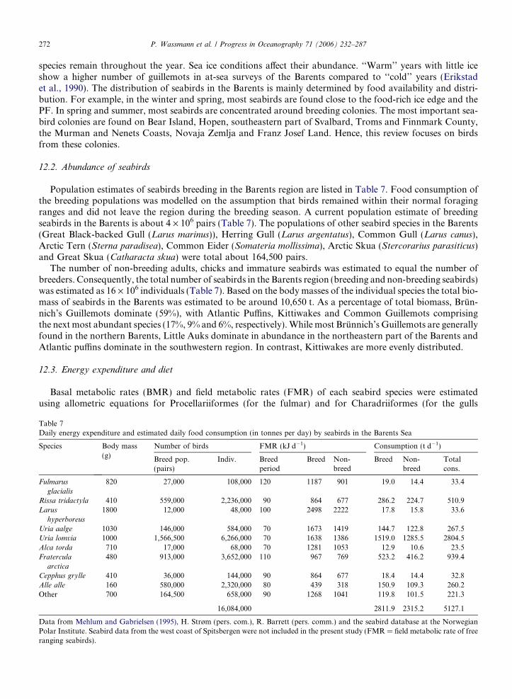
272 P. Wassmann et al. / Progress in Oceanography 71 (2006) 232–287
species remain throughout the year. Sea ice conditions affect their abundance. ‘‘Warm’’ years with little iceshow a higher number of guillemots in at-sea surveys of the Barents compared to ‘‘cold’’ years (Erikstadet al., 1990). The distribution of seabirds in the Barents is mainly determined by food availability and distri-bution. For example, in the winter and spring, most seabirds are found close to the food-rich ice edge and thePF. In spring and summer, most seabirds are concentrated around breeding colonies. The most important sea-bird colonies are found on Bear Island, Hopen, southeastern part of Svalbard, Troms and Finnmark County,the Murman and Nenets Coasts, Novaja Zemlja and Franz Josef Land. Hence, this review focuses on birdsfrom these colonies.
12.2. Abundance of seabirds
Population estimates of seabirds breeding in the Barents region are listed in Table 7. Food consumption ofthe breeding populations was modelled on the assumption that birds remained within their normal foragingranges and did not leave the region during the breeding season. A current population estimate of breedingseabirds in the Barents is about 4 · 106 pairs (Table 7). The populations of other seabird species in the Barents(Great Black-backed Gull (Larus marinus)), Herring Gull (Larus argentatus), Common Gull (Larus canus),Arctic Tern (Sterna paradisea), Common Eider (Somateria mollissima), Arctic Skua (Stercorarius parasiticus)and Great Skua (Catharacta skua) were total about 164,500 pairs.
The number of non-breeding adults, chicks and immature seabirds was estimated to equal the number ofbreeders. Consequently, the total number of seabirds in the Barents region (breeding and non-breeding seabirds)was estimated as 16 · 106 individuals (Table 7). Based on the body masses of the individual species the total bio-mass of seabirds in the Barents was estimated to be around 10,650 t. As a percentage of total biomass, Brun-nich’s Guillemots dominate (59%), with Atlantic Puffins, Kittiwakes and Common Guillemots comprisingthe next most abundant species (17%, 9% and 6%, respectively). While most Brunnich’s Guillemots are generallyfound in the northern Barents, Little Auks dominate in abundance in the northeastern part of the Barents andAtlantic puffins dominate in the southwestern region. In contrast, Kittiwakes are more evenly distributed.
12.3. Energy expenditure and diet
Basal metabolic rates (BMR) and field metabolic rates (FMR) of each seabird species were estimatedusing allometric equations for Procellariiformes (for the fulmar) and for Charadriiformes (for the gulls
Table 7Daily energy expenditure and estimated daily food consumption (in tonnes per day) by seabirds in the Barents Sea
Species Body mass(g)
Number of birds FMR (kJ d�1) Consumption (t d�1)
Breed pop.(pairs)
Indiv. Breedperiod
Breed Non-breed
Breed Non-breed
Totalcons.
Fulmarus
glacialis
820 27,000 108,000 120 1187 901 19.0 14.4 33.4
Rissa tridactyla 410 559,000 2,236,000 90 864 677 286.2 224.7 510.9Larus
hyperboreus
1800 12,000 48,000 100 2498 2222 17.8 15.8 33.6
Uria aalge 1030 146,000 584,000 70 1673 1419 144.7 122.8 267.5Uria lomvia 1000 1,566,500 6,266,000 70 1638 1386 1519.0 1285.5 2804.5Alca torda 710 17,000 68,000 70 1281 1053 12.9 10.6 23.5Fratercula
arctica
480 913,000 3,652,000 110 967 769 523.2 416.2 939.4
Cepphus grylle 410 36,000 144,000 90 864 677 18.4 14.4 32.8Alle alle 160 580,000 2,320,000 80 439 318 150.9 109.3 260.2Other 700 164,500 658,000 90 1268 1041 119.8 101.5 221.3
16,084,000 2811.9 2315.2 5127.1
Data from Mehlum and Gabrielsen (1995), H. Strøm (pers. com.), R. Barrett (pers. comm.) and the seabird database at the NorwegianPolar Institute. Seabird data from the west coast of Spitsbergen were not included in the present study (FMR = field metabolic rate of freeranging seabirds).
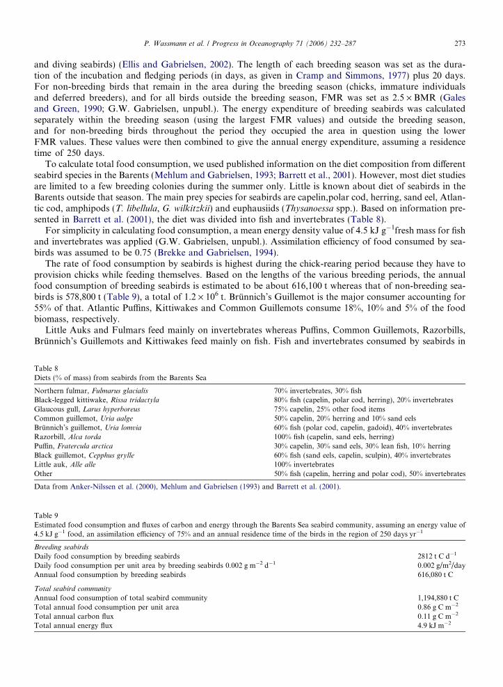
P. Wassmann et al. / Progress in Oceanography 71 (2006) 232–287 273
and diving seabirds) (Ellis and Gabrielsen, 2002). The length of each breeding season was set as the dura-tion of the incubation and fledging periods (in days, as given in Cramp and Simmons, 1977) plus 20 days.For non-breeding birds that remain in the area during the breeding season (chicks, immature individualsand deferred breeders), and for all birds outside the breeding season, FMR was set as 2.5 · BMR (Galesand Green, 1990; G.W. Gabrielsen, unpubl.). The energy expenditure of breeding seabirds was calculatedseparately within the breeding season (using the largest FMR values) and outside the breeding season,and for non-breeding birds throughout the period they occupied the area in question using the lowerFMR values. These values were then combined to give the annual energy expenditure, assuming a residencetime of 250 days.
To calculate total food consumption, we used published information on the diet composition from differentseabird species in the Barents (Mehlum and Gabrielsen, 1993; Barrett et al., 2001). However, most diet studiesare limited to a few breeding colonies during the summer only. Little is known about diet of seabirds in theBarents outside that season. The main prey species for seabirds are capelin,polar cod, herring, sand eel, Atlan-tic cod, amphipods (T. libellula, G. wilkitzkii) and euphausiids (Thysanoessa spp.). Based on information pre-sented in Barrett et al. (2001), the diet was divided into fish and invertebrates (Table 8).
For simplicity in calculating food consumption, a mean energy density value of 4.5 kJ g�1fresh mass for fishand invertebrates was applied (G.W. Gabrielsen, unpubl.). Assimilation efficiency of food consumed by sea-birds was assumed to be 0.75 (Brekke and Gabrielsen, 1994).
The rate of food consumption by seabirds is highest during the chick-rearing period because they have toprovision chicks while feeding themselves. Based on the lengths of the various breeding periods, the annualfood consumption of breeding seabirds is estimated to be about 616,100 t whereas that of non-breeding sea-birds is 578,800 t (Table 9), a total of 1.2 · 106 t. Brunnich’s Guillemot is the major consumer accounting for55% of that. Atlantic Puffins, Kittiwakes and Common Guillemots consume 18%, 10% and 5% of the foodbiomass, respectively.
Little Auks and Fulmars feed mainly on invertebrates whereas Puffins, Common Guillemots, Razorbills,Brunnich’s Guillemots and Kittiwakes feed mainly on fish. Fish and invertebrates consumed by seabirds in
Table 8Diets (% of mass) from seabirds from the Barents Sea
Northern fulmar, Fulmarus glacialis 70% invertebrates, 30% fishBlack-legged kittiwake, Rissa tridactyla 80% fish (capelin, polar cod, herring), 20% invertebratesGlaucous gull, Larus hyperboreus 75% capelin, 25% other food itemsCommon guillemot, Uria aalge 50% capelin, 20% herring and 10% sand eelsBrunnich’s guillemot, Uria lomvia 60% fish (polar cod, capelin, gadoid), 40% invertebratesRazorbill, Alca torda 100% fish (capelin, sand eels, herring)Puffin, Fratercula arctica 30% capelin, 30% sand eels, 30% lean fish, 10% herringBlack guillemot, Cepphus grylle 60% fish (sand eels, capelin, sculpin), 40% invertebratesLittle auk, Alle alle 100% invertebratesOther 50% fish (capelin, herring and polar cod), 50% invertebrates
Data from Anker-Nilssen et al. (2000), Mehlum and Gabrielsen (1993) and Barrett et al. (2001).
Table 9Estimated food consumption and fluxes of carbon and energy through the Barents Sea seabird community, assuming an energy value of4.5 kJ g�1 food, an assimilation efficiency of 75% and an annual residence time of the birds in the region of 250 days yr�1
Breeding seabirds
Daily food consumption by breeding seabirds 2812 t C d�1
Daily food consumption per unit area by breeding seabirds 0.002 g m�2 d�1 0.002 g/m2/dayAnnual food consumption by breeding seabirds 616,080 t C
Total seabird community
Annual food consumption of total seabird community 1,194,880 t CTotal annual food consumption per unit area 0.86 g C m�2
Total annual carbon flux 0.11 g C m�2
Total annual energy flux 4.9 kJ m�2
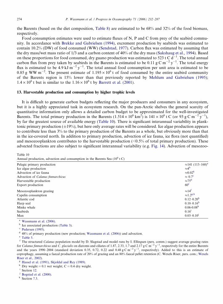
274 P. Wassmann et al. / Progress in Oceanography 71 (2006) 232–287
the Barents (based on the diet composition, Table 8) are estimated to be 68% and 32% of the food biomass,respectively.
Food consumption estimates were used to estimate fluxes of N, P and C from prey of the seabird commu-nity. In accordance with Brekke and Gabrielsen (1994), excrement production by seabirds was estimated tocontain 10.2% (DW) of food consumed (WW) (Sendstad, 1977). Carbon flux was estimated by assuming thatthe dry mass/wet mass ratio of 1/3 and a carbon content of 40% of the dry mass (Sakshaug et al., 1994). Basedon these proportions for food consumed, dry guano production was estimated to 523 t C d�1. The total annualcarbon flux from prey taken by seabirds in the Barents is estimated to be 0.11 g C m�2 y�1. The total energyflux is estimated to be 4.9 kJ m�2 y�1. The total annual food consumption per unit area is estimated to be0.85 g WW m�2. The present estimate of 1.195 · 106 t of food consumed by the entire seabird communityof the Barents region is 15% lower than that previously reported by Mehlum and Gabrielsen (1995);1.4 · 106 t but is similar to the 1.16 · 106 t by Barrett et al. (2001).
13. Harvestable production and consumption by higher trophic levels
It is difficult to generate carbon budgets reflecting the major producers and consumers in any ecosystem,but it is a highly appreciated task in ecosystem research. On the pan-Arctic shelves the general scarcity ofquantitative information only allows a detailed carbon budget to be approximated for the well-investigatedBarents. The total primary production in the Barents (1.514 · 106 km2) is 141 · 106 t C (or 93 g C m�2 y�1),by far the greatest source of available energy (Table 10). There is significant interannual variability in plank-tonic primary production (±19%), but here only average rates will be considered. Ice algae production appearsto contribute less than 3% to the primary production of the Barents as a whole, but obviously more than thatin the ice-covered north. In addition to primary production, advection of ice fauna, ice flora (not quantified)and mesozooplankton contributes to the harvestable production (<0.5% of total primary production). Theseadvected fractions are also subject to significant interannual variability (e.g. Fig. 14). Advection of mesozoo-
Table 10Annual production, advection and consumption in the Barents Sea (106 t C)
Pelagic primary production �141 (113–168)a
Ice algae production �4b
Advection of ice fauna �0.02k
Advection of Calanus finmarchicus � 0.7c
Harvestable production �75d
Export production 60e
Mesozooplankton grazing �14f
Capelin consumption �1.2g,h
Atlantic cod 0.12–0.20h
Harp seal 0.10–0.16h
Minke whale 0.06-0.08h
Seabirds 0.16i
Man 0.03–0.10j
a Wassmann et al. (2006).b Ice associated production (Table 3).c Pedersen (1995).d 48% of primary production (new production; Wassmann et al. (2006)) and advection.e Table 5.f The structured Calanus population model by D. Slagstad and model runs by I. Ellingsen (pers. comm.) suggest average grazing rates
for Calanus finmarchicus and C. glacialis on diatoms and ciliates of 1.87, 2.33, 1.7 and 2.17 g C m�2 y�1, respectively for the entire Barentsand the years 1990–2004 (standard deviation 0.35, 0.72, 0.22 and 0.48 g C m�2 y�1, respectively). Added to this is an estimate ofcoprophagy, assuming a faecal production rate of 20% of grazing and an 80% faecal pellet retention (C. Wexels Riser, pers. com.; WexelsRiser et al., 2002).
g Hassel et al. (1991), Skjoldal and Rey (1989).h Dry weight = 0.1 wet weight; C = 0.4 dry weight.i Section 12.j Bogstad et al. (2000).
k Section 7.3.
P. Wassmann et al. / Progress in Oceanography 71 (2006) 232–287 275
plankton comprises by far the greatest share (0.46 g C m�2 y�1) and is most important in the southwesternBarents. About 75 · 106 t C (or 50 g C m�2 y�1), i.e. 50% of the total primary production is harvestableand can be channelled into the pelagic and benthic food webs (Table 10). The export production estimateis probably the most fragile of all estimates in Table 10. It suggests that 60 · 106 t C (40 g C m�2 y�1) areannually injected into the >100 m layer, feeding deep-dwelling zooplankton and benthos (such as the econom-ically important, epibenthic Pandalus borealis). Table 10 indicates further that the most of the harvestable pro-duction is not channelled into the upper 100 m planktonic community, but into deep-dwelling zooplanktonand benthos. Despite the fact that much of the high-quality food is channelled through the planktonic foodweb to higher trophic levels, 80% of the harvestable carbon is supplied to deeper water and the sediment,implying that remineralisation of nutrients is far greater in this realm than in the upper water column.
The difference between the harvestable and export production comes close to the zooplankton grazing esti-mate of 14 106t C, or 9.2 g C m�2 (Table 10). It is first of all the mesozooplankton production that creates thefood base for the higher trophic levels, sea birds and the commercial species of the Barents, one of the world’slargest fisheries. How much of the harvestable production do fish and higher trophic levels consume? About19% is channelled through the key mesozooplankton species C. finmarchicus and C. glacialis. Capelin (andherring?) consumes much of the zooplankton standing stock in the SIZ, in particular south of the PF. Theirenergy consumption is about 10% of that of their main food, mesozooplankton (Table 10). However, this is aparticularly vague estimate as capelin stocks vary significantly over time, competing with herring for the samekey food source, while both stocks are subjected to fisheries. Capelin channels 1.6% of the harvestable produc-tion from the pelagic of the Barents to the many species that depend on it (Table 10). In comparison to earlierestimates for the Barents (e.g. in Walsh and Sakshaug, 2000) the consumption rates presented here are con-siderably higher. We interpret this by the fact that most of the present consumption rates are based upondetailed and laborious stomach analyses that were not available previously.
Less than 1% of the harvestable production is channelled through cod, harp seals, minke whales, sea birdsand man. Cod is the greatest consumer of invertebrates and fish, followed by harp seals, minke whales, seabirds and man. Man extracts only a fraction of the harvestable energy passing through invertebrates. The fishand fisheries fractions are of the same order of magnitude as other higher trophic levels. Thus, cod, seals,whales and man compete for harvestable energy with a similar intensity. Climate variability and change, dif-ferences in recruitment, variable resource availability, harvesting restrictions and management schemes willinfluence the ratio between these competitors. For the various groups, there are significant interannual differ-ences in consumption and production, as reflected by the variable food consumption by cod (Fig. 22). Present-ing averages like those in Table 10 gives, thus, only a rough impression of the proportions of the mostimportant players in the Barents food web.
14. Climate and food web changes: an outlook
The considerable climate variability in the Barents conceals the direct and immediate signs of global warm-ing that are far more prevalent in other Arctic regions, for example in the Bering Sea–Bering Strait, Chukchiand Beaufort Sea regions (e.g. Hunt et al., 2002; Grebmeier et al., 2006). However, in the period 1920–1998,for which there are nearly continuous April and August ice edge observations, an overall ice extent shrinkageis observed for April and August of about 12% and 40%, respectively (Vinje, 2001). This large difference in iceextent is reflected in the net increase in the Spitsbergen seasonal temperatures over the corresponding period(winter +1 �C, spring and summer +0.5 �C, autumn 0.0 �C; Hanssen-Bauer, 2002). The large difference in win-ter vs. summer ice shrinkage suggests that recent warming has had a far higher impact on ice disintegrationthan on the seasonal freezing rate. Connections among weather, climate, the state of the Arctic ice coverand inflow of AW into the Barents have been established (Grønas and Skeie, 1999; Lopez et al., 2000; Ottersenet al., 2000). It is, thus, of fundamental importance to understand how annual, interannual and decadal vari-ations in ice extent are related to climate forcing (e.g. NAO, AO) and the shelf seas fringing the AO.
Preliminary forecasts (Johannessen et al., 2002) indicate a reduction of the Polar ice pack of 20% duringwinter and 80% during summer by the end of this century. The dramatic northward retreat of the MIZ duringthe productive season will result in a profound widening of the SIZ and result in an extensive, stratified areathat stretching from the Barents well into the AO deep basin. As a consequence, primary production will
276 P. Wassmann et al. / Progress in Oceanography 71 (2006) 232–287
increase and a substantial proportion of primary production that currently fuels the shelf system will be ‘‘lost’’to the deep AO system.
Also northward shifts of biogeographic boundaries are inevitable with continued warming of the Barents.Recently, the boreal mussel, Mytilus edulis, a key stone species in temperate waters, was discovered in Sval-bard after a 1000 years absence (Berge et al., 2005). This exemplifies the potential for significant and non-pre-dictable alterations from invasive species previously excluded by the unfavourable conditions. As aconsequence, the function of the food web of the Barents ecosystem may be changed by continuous warmingand sea ice retreat as well as the invasion of boreal species such as e.g. M. edulis, mackerel and blue whiting(Micromesistius poutassou) or by introduced species such as the king crab (Paralithodes camtschaticus).
The predicted changes in the earth’s climate (IPCC, 2001) are expected to be amplified in polar areas(IPCC, 1998; Weller and Lange, 1999; ACIA, 2001, 2004). Because of the control of sea ice on primary pro-duction and on pelagic benthic coupling, and because of the physical properties of ice as a habitat for marineflora and fauna, the dynamics of ice cover act as a pivot point through which changes in climatic patterns aretranslated to the marine ecosystem. A warmer Arctic, with less sea ice, will probably have a more than 30%greater overall primary production (Wassmann et al., 2006) with a relatively greater contribution from pelagicplankton at the expense of ice algae (Horner and Schrader, 1982; Hsiao, 1992; Legendre et al., 1992). Theseclimate-induced changes can have profound impacts on the trophic structure and energy flow of the coupledice-pelagic–benthic system (Carroll and Carroll, 2003). Ice algae-derived biogenic matter is a part of the sur-face sediment in the Barents (Tamelander et al., 2005), and benthic fauna readily consume ice algae. They mayprefer it as a food source compared to phytoplankton (McMahon et al., 2006). Furthermore, in certain areas ahigher proportion of ice algal production may sediment to the sea bottom compared to phytoplankton (seeSection 3). These factors suggest that the loss of sea ice and the concomitant changes in the production cycle(i.e. a loss of sea ice algal production in favour of open water primary production) may generally bolster thepelagic system at the expense of the benthic component.
Continued reduction of the ice extent in the northern Barents will have negative consequences for highertrophic levels that depend on ice-associated flora and fauna and ice as habitat. Earlier melting will causereduced availability of ice fauna to predators during the summer and autumn. Reduction in ice transport intothe Barents will reduce biomass import, with consequences for the carbon export to the benthos in the north.The Barents may develop from a SIZ into an oceanic shelf system, possibly with threefold higher pelagic pro-duction (Reigstad et al., 2002; Sakshaug, 2004), marginalizing the contribution of ice-associated flora andfauna. An important component of this increase in productivity is de-stratification, giving raise to increasednutrient supply by wind-induced vertical mixing (Wassmann et al., 2006). All this will lead to an atlantification
(sensu Wassmann et al., 2004) of the northern Barents in decades to come.The non-linear nature of ecosystem changes prevents more specific predictions about the trajectories of
food web changes. Climate-induced ecosystem changes, e.g. the invasion of new key species, may result inchanges in ecosystem function that may make the ecosystem representation in current models invalid. Projec-tions into a warmer future, based upon the present ecosystem understanding, are thus questionable. We final-ise our account on the food webs of the Barents by focussing upon two graphic representations of coastal andoffshore pelagic ecosystems supporting higher trophic levels. In the ArW surrounding Svalbard, the cold-watercalanoid copepods C. glacialis and C. hyperboreus are pelagic keystone species (Fig. 23a). They carry the bio-geochemical signature of diatoms that usually bloom in this region in May. The Little Auk, one of the pre-dominant birds breeding along the Svalbard coast, feeds upon these copepods in surface waters(Karnovsky et al., 2003). The harvestable energy derived from the lower trophic level dynamics, which areshaped by processes such as ice-cover, warming and vertical mixing, is thus directly transferred to higher tro-phic levels. A different situation is encountered in the SIZ of the open Barents, often ice-free and dominated byAW (Fig. 23b). Primary production starts earlier and is channelled into the keystone calanoid copepod C.
finmarchicus that in turn is the prime food for capelin and herring. Migrating mammals such as minke whalesfeed upon these pelagic fish resources in the later part of the productive season. An atlantification of the ArWregions off Svalbard would deprive the Little Auk population of its feeding grounds, resulting in decreasedbreeding success, followed by a replacement by pelagic fish and migrating mammals. In the Barents, atlantif-ication would imply both higher food potential for some pelagic fish and mammals and northward extensionof feeding grounds.
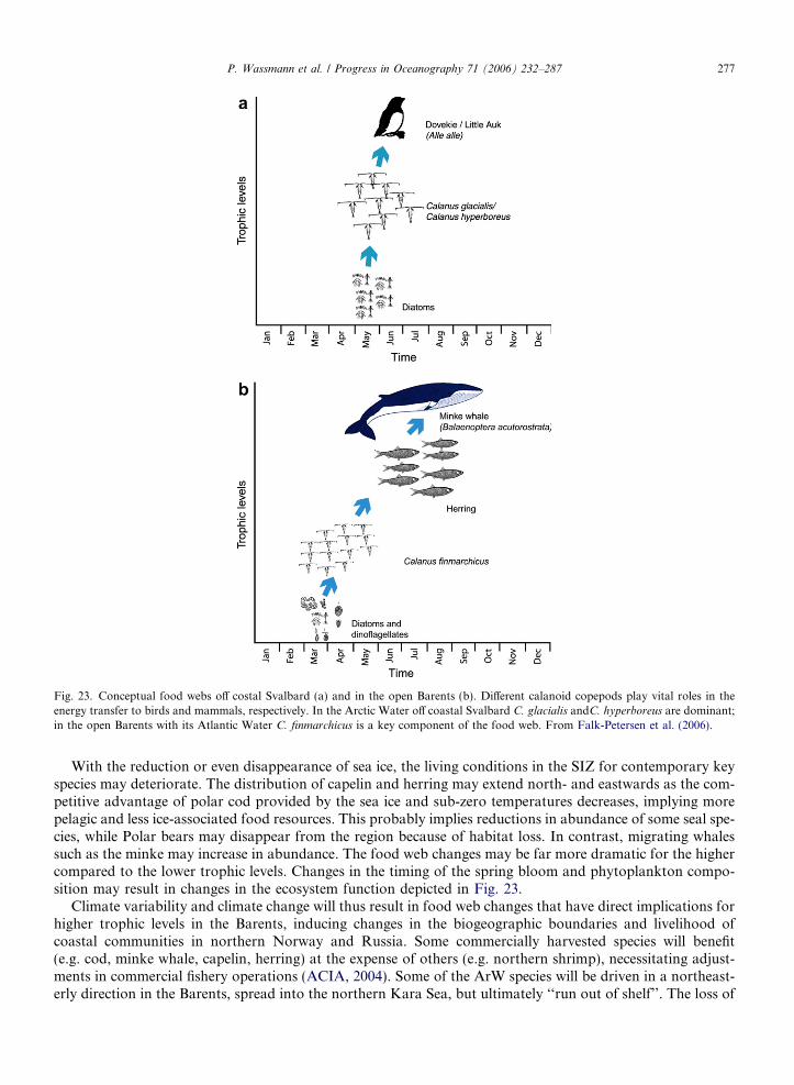
Fig. 23. Conceptual food webs off costal Svalbard (a) and in the open Barents (b). Different calanoid copepods play vital roles in theenergy transfer to birds and mammals, respectively. In the Arctic Water off coastal Svalbard C. glacialis andC. hyperboreus are dominant;in the open Barents with its Atlantic Water C. finmarchicus is a key component of the food web. From Falk-Petersen et al. (2006).
P. Wassmann et al. / Progress in Oceanography 71 (2006) 232–287 277
With the reduction or even disappearance of sea ice, the living conditions in the SIZ for contemporary keyspecies may deteriorate. The distribution of capelin and herring may extend north- and eastwards as the com-petitive advantage of polar cod provided by the sea ice and sub-zero temperatures decreases, implying morepelagic and less ice-associated food resources. This probably implies reductions in abundance of some seal spe-cies, while Polar bears may disappear from the region because of habitat loss. In contrast, migrating whalessuch as the minke may increase in abundance. The food web changes may be far more dramatic for the highercompared to the lower trophic levels. Changes in the timing of the spring bloom and phytoplankton compo-sition may result in changes in the ecosystem function depicted in Fig. 23.
Climate variability and climate change will thus result in food web changes that have direct implications forhigher trophic levels in the Barents, inducing changes in the biogeographic boundaries and livelihood ofcoastal communities in northern Norway and Russia. Some commercially harvested species will benefit(e.g. cod, minke whale, capelin, herring) at the expense of others (e.g. northern shrimp), necessitating adjust-ments in commercial fishery operations (ACIA, 2004). Some of the ArW species will be driven in a northeast-erly direction in the Barents, spread into the northern Kara Sea, but ultimately ‘‘run out of shelf’’. The loss of
278 P. Wassmann et al. / Progress in Oceanography 71 (2006) 232–287
adequate summer ice will cause Polar bears to loose their feeding grounds after overwintering and breeding inthe Barents region. Finally, amplifications of the warming in the Arctic will impact wildlife on a global levelbecause long-distance animal migration routes (e.g. whales and birds) are sensitive to local changes in habitatand food availability in the Barents.
Acknowledgements
This publication was supported by the Nordic Arctic Research Program (NARP) project Climate change,
carbon flux and living resources in the Nordic Sea, the NordForsk network Arktiske økosystemer, karbon fluks
og klimatisk forandring and the Research Council of Norway (Nordklima) projects Carbon flux and ecosystem
feed back in the northern Barents Sea in an era of climate change (CABANERA), Marine climate and ecosys-
tems in the seasonal ice zone (MACESIZ), and On thin ice: Climatic influence on energy flow and trophic struc-ture in arctic marine ecosystems. The writing of this paper was supported in part by the Norwegian ResearchCouncil, grant numbers 150356-720 to M. L. Carroll, and 155936-700 to P. Wassmann.
We thank two anonymous referees for their comments and suggestions. We thank Scott Shaffer, Univer-sity of California, and Rob Barret, University of Tromsø, for their constructive comments on the manu-script. Thanks to Frøydis Strand for support with the figures. This manuscript was partly written duringa sabbatical at the Universite Laval, Quebec, Canada, and P.W. wishes to thank Louis Fortier for thehospitality.
Without the vision, dedication and firm leadership of Egil Sakshaug during the Pro Mare project (1984-1990) much of the recent research in the Barents would not have been carried out in a system ecological per-spective and with the dedicated goal to understand the functional and holistic aspects of this ecosystem.
References
Aagaard, K., Greisman, P., 1975. Towards a new mass and heat budget for the Arctic Ocean. Journal of Geophysical Research 80, 3821–3827.
Aarefjord, H., Bjørge, A.J, Kinze, C.C., Lindstedt, I., 1995. Diet of the harbour porpoise (Phocoena phocoena) in Scandinavian waters.Report International Whaling Commission, Special issue 16, pp. 211-222.
ACIA, 2001. Report from the Arctic Climate Impact Assessment Modelling and Scenarios Workshop, Stockholm, January 29–31.Available from: <http://www.srrb.noaa.gov/UV/arctic.html>.
ACIA, 2004. Impacts of a Warming Arctic: Arctic Climate Impact and Assessment. Cambridge University Press, Cambridge, 144pp.Adlandsvik, B., Loeng, H., 1991. A study of the climatic system in the Barents Sea. Polar Research 10, 45–49.Ajiad, A.M., Gjøsæter, H., 1990. Diet of polar cod, Boreogadus saida, in the Barents Sea related to fish size and geographical distribution.
International Council for the Exploration of the Sea, Council Meeting 1990/G:48, 9pp.Aksnes, D.L., Wassmann, P., 1993. Modelling the significance of zooplankton grazing for export production. Limnology and
Oceanography 38, 978–985.Ambrose Jr., W.G., von Quillfeldt, C.H., Clough, L.M., Tilney, P.V.R., Tucker, P., 2005. The sub-ice algal community in the Chukchi
Sea: large- and small-scale patterns of abundance based on images from a remotely operated vehicle. Polar Biology 28, 784–795.Ambrose, W.G., Carroll, M.L., Greenacre, M., Thorrold, S., McMahon, K., 2006. Variation in Serripes groenlandicus (Bivalvia) growth in
a Norwegian high-Arctic fjord: evidence for local- and large-scale climatic forcing. Global Change Biology 12, 1595–1607.Andersen, C., Koc, N., Moros, M., 2004. A highly unstable Holocene climate in the subpolar North Atlantic: evidence from diatoms.
Quaternary Science 23 (20–22), 2155–2166.Anderson, L.G., Jones, E.P., Lindegren, R., Rudels, B., Sehlstedt, P.-I., 1988. Nutrient regeneration in cold, high salinity bottom water of
the Arctic shelves. Continental Shelf Research 8, 1345–1355.Andreassen, I.J., Wassmann, P., 1998. Vertical flux of phytoplankton and particulate biogenic matter in the marginal ice zone of the
Barents Sea in May 1993. Marine Ecology Progress Series 170, 1–14.Andreassen, I., Nothig, E.-M., Wassmann, P., 1996. Vertical particle flux on the shelf off northern Spitsbergen, Norway. Marine Ecology
Progress Series 137, 215–228.Anker-Nilssen, T., Bakken, V., Strøm, H., Golovkin, A.N., Bianki, V.V., Tatarinkova, I.P. (Eds.), 2000. The status of marine birds
breeding in the Barents Sea region. Norsk Polarinstitutt Rapportserie, vol. 113, Tromsø, 213pp.Antipova, T.V., 1975. Benthos biomass distribution of the Barents Sea. Trudy PINRO 35, 121–124 (in Russian).Arashkevich, E., Wassmann, P., Pasternak, A., Riser, C.W., 2002. Seasonal and spatial changes in biomass, structure, and development
progress of the zooplankton community in the Barents Sea. Journal of Marine Systems 38, 125–145.Arndt, C., Lønne, O.J., 2002. Transport of bioenergy by large scale Arctic ice drift. In: Ice in the environment: Proceedings of the 16th
IAHR International Symposium on Ice Dunedin, New Zealand. International Association of Hydraulic Engineering and Research, pp.103–111.
P. Wassmann et al. / Progress in Oceanography 71 (2006) 232–287 279
Barrett, R.T., Anker-Nilssen, T., Gabrielsen, G.W., Chapdelaine, G., 2001. Food consumption by seabirds in Norwegian waters. ICESJournal of Marine Science 59, 43–57.
Belikov, S.E., Boltunov, A.N., 1998. The ringed seal (Phoca hispida) in the western Russian Arctic. NAMMCO Scientific Publication 1,63–82.
Berge, J., Johnsen, G., Nilsen, F., Gulliksen, B., Slagstad, D., 2005. Ocean temperature oscillations enforce the reappearance of bluemussels in Svalbard after 1000 years of absence. Marine Ecology Progress Series 303, 167–175.
Berg, I., Haug, T., Nilssen, K.T., 2002. Harbour seal (Phoca vitulina) diet in Vesteralen, north Norway. Sarsia 87, 451–461.Beuchel, F., Gulliksen, B., Carroll, M.L., 2006. Long-term patterns (1980–2003) of rocky-bottom macrobenthic community structure in an
Arctic fjord (Kongsfjorden, Svalbard) in relation to climate variability. Journal of Marine Systems, in press, doi:10.1016/j.jmarsys.2006.05.002.
Bjørge, A.J., Øien, N., 1995. Distribution and abundance of harbour porpoise, Phocoena phocoena, in Norwegian waters. ReportsInternational Whaling Commission, Special issue 16, pp. 89–98.
Bjørge, A., Øien, N., 1999. Statusrapport for Havforskningsinstituttets overvakning av kystsel. Havforskningsinstituttet Rappport SPS-9904, 35pp. (in Norwegian).
Blindheim, J., 1989. Ecological features of the Norwegian Sea. In: Rey, L., Alexander, V. (Eds.) Proceedings of the Sixth Conference of theComitee Arctique International, Brill, Leiden, pp. 366–401.
Bogorov, V.G., Vinogradov, M.E., Voronina, N.M., Kanaeva, I.P., Suetova, I.A., 1968. Distribution of zooplankton biomass in the upperlayer of the World Ocean. Doklady AS USSR 182, 1205–1207 (in Russian).
Bogstad, B., Gjøsæter, H., 2001. Predation by cod (Gadus morhua) on capelin (Mallotus villosus) in the Barents Sea: implications forcapelin stock assessment. Fisheries Research 53, 197–209.
Bogstad, B., Mehl, S., 1997. Interactions between Atlantic cod (Gadus morhua) and its prey species in the Barents Sea. In: Proceedings.Forage Fishes in Marine Ecosystems. Alaska Sea Grant College Program Report No. 97-01, University of Alaska Fairbanks, pp. 591–615.
Bogstad, B., Haug, T., Mehl, S., 2000. Who eats whom in the Barents Sea? NAMMCO Scientific Publication 2, 65–80.Boldovsky, G.V., 1944. Feeding of the Barents Sea redfish. Trudy PINRO 8, 307–330 (in Russian).Born, E., Gjertz, I., Reeves, R.R., 1995. Population assessment of Atlantic walrus (Odobenus rosmarus rosmarus L.). Norsk Polarinstitutt
Meddelelser 138, 100pp (in Norwegian).Bowen, W.D., 1997. Role of marine mammals in aquatic ecosystems. Marine ecology Progress Series 158, 267–274.Bradstreet, M.S.W., Cross, W.E., 1982. Trophic relationships at high-arctic ice edges. Arctic 35, 1–12.Brekke, B., Gabrielsen, G.W., 1994. Assimilation efficiency of adult kittiwakes and Brunnich’s guillemots fed capelin and arctic cod. Polar
Biology 14, 279–284.Burgos, G., Mehl, S., 1987. Diet overlap between North-east Arctic cod and haddock in the Southern Barents Sea. International Council
for the Exploration of the Sea, Council Meeting 1987/G:50, 22pp.Cairns, D.K., Chapdelaine, G., Montevecchi, W.A., 1991. Prey exploitation by seabirds in the Gulf of St. Lawrence. Canadian Special
Publication of Fisheries and Aquatic Science 113, 277–291.Carmack, E., Barber, D., Christensen, J., Macdonald, R., Rudels, B., Sakshaug, E., 2006. Climate variability and physical forcing of the
food webs and the carbon budget on panarctic shelves. Progress in Oceanography (this volume).Carroll, M.L., Carroll, J., 2003. The Arctic seas. In: Black, K., Shimmield, G. (Eds.), Biogeochemistry of Marine Systems. Blackwell
Publishing Ltd., Oxford, pp. 127–156.Carroll, M.L., Pearson, T., Dragsund, E., Gabrielsen, K.L., 2000. Environmental status of the Norwegian offshore sector based on the
petroleum regional monitoring programme, 1996–1998. The Norwegian Oil Industry Association Report, APN 411.1777.04, 39pp.ISBN: 82-449-0053-9.
Christensen, I., 1982. Killer whales in Norwegian coastal waters. Reports International Whaling Commission 32, 633–672.Christensen, I., Haug, T., Øien, N., 1992a. Seasonal distribution, exploitation and present abundance of stocks of large baleen whales
(Mysticeti) and sperm whales (Physeter macrocephalus) in Norwegian and adjacent waters. ICES Journal of Marine Sciences 49, 341–355.
Christensen, I., Haug, T., Øien, N., 1992b. A review of feeding and reproduction in large baleen whales (Mysticeti) and sperm whalesPhyseter macrocephalus in Norwegian and adjacent waters. Fauna Norvegica, Series A 13, 39–48.
Cleve, P.T., 1899. Plankton collected by the Swedish expedition to Spitzbergen in 1898. Kongelig Svenska Vetenskapsakademi Handlingar32, 1–48.
Cleve, P.T., Grunnow, A., 1880. Beitrage zur Kenntnis der Arctischen Diatomeen. Kongelig Svenska Vetenskapsakademi Handlingar 17,1–21.
Coppola, L., Roy-Barman, M., Wassmann, P., Mulsow, S., Jeandel, C., 2002. Calibration of sediment traps and particulate organiccarbon export using 234Th in the Barents Sea. Marine Chemistry 80, 11–26.
Corkeron, P.J., Connor, R.C., 1999. Why do baleen whales migrate? Marine Mammalian Science 15, 1228–1254.Cramp, S., Simmons, K.E.L. (Eds.), 1977. The Birds of the Western Palearctic. Handbook of the Birds of Europe, the Middle East and
North Africa. Ostrich to Ducks, vol. I. Oxford University Press, Oxford, p. 722.Croll, D.A., Maron, J.L., Estes, J.A., Danner, E.M., Byrd, G.V., 2005. Introduced predators transform subarctic islands from grassland to
tundra. Science 307, 1959–1961.Curtis, M.A., 1975. The marine benthos of the Arctic and sub-Arctic continental shelves: a review of regional studies and their general
results. Polar Record 17, 595–626.Dahle, S., Denisenko, S.D., Denisenko, N.V., Cochrane, S., 1998. Benthic fauna in the Pechora Sea. Sarsia 83, 183–210.
280 P. Wassmann et al. / Progress in Oceanography 71 (2006) 232–287
Dahl, T.M., Lydersen, C., Kovacs, K.M., Falk-Petersen, S., Sargent, J., Gjertz, I., Gulliksen, B., 2000. Fatty acid composition of theblubber in white whales (Delphinapterus leucas). Polar Biology 23, 401–409.
Dalpadado, P., Borkner, N., Bogstad, B., Mehl, S., 2001. Distribution of Themisto (Amphipoda) spp. in the Barents Sea and predator-prey interactions. ICES Journal of Marine Science 58, 876–895.
Defant, A., 1949. Konvektion und Eisbereitschaft in polaren Eismeeren. Geografiska Annaler, Stockholm.Defant, A., 1961Physical oceanography, vol. I. Pergamon Press, Oxford, 729pp.Degtereva, A.A., 1973. The relationship between abundance and biomass of plankton and the temperature in the south-western part of the
Barents Sea. Trudy PINRO 33, 13–23 (in Russian).Denisenko, S.G., 2001. Long-term changes of zoobenthos biomass in the Barents Sea. Proceedings of the Zoological Institute, Russian
Academy of Sciences 289, 59–66.Denisenko, S.G., 2002. Zoobenthos and ice distribution in the Arctic seas. Proceedings of the Zoological Institute, Russian Academy of
Sciences 296, 39–46.Denisenko, S.G., 2004. Structurally-functional characteristics of the Barents Sea zoobenthos. Proceedings of the Zoological Institute,
Russian Academy of Sciences 300, 43–52.Denisenko, S.G., Denisenko, N.V., 2003. Long-term changes of zoobenthos biomass in the Pechora Sea as an indicator of climate
variability. In: Arctic Climate System Study (ACSYS) Final Science Conference, St. Petersburg, Russia (extended abstract).Denisenko, S.G., Tytov, O.V., 2003. Distribution of zoobenthos and primary plankton production in the Barents Sea. Oceanology 43, 78–
88 (in Russian).Denisenko, S.G., Denisenko, N.V., Lehtonen, K.K., Andersin, A.-B., Laine, A.O., 2003. Macro-zoobenthos of the Pechora Sea
(southeastern Barents Sea): community structure and spatial distribution in relation to environmental conditions. Marine EcologyProgress Series 258, 109–123.
Diel, S., Tande, K.S., 1991. Does the spawning of Calanus finmarchicus in high latitudes follow a reproducible pattern? Marine Biology113, 21–31.
Dolgov, A.V., 1997. Distribution, abundance, biomass and feeding of thorny skate, Raja radiata, in the Barents Sea. International Councilfor the Exploration of the Sea, Council Meeting 1997/GG:04, 21pp.
Dolgov, A.V., 2002. The role of capelin (Mallotus villosus) in the foodweb of the Barents Sea. ICES Journal of Marine Science 59, 1034–1045.
Dolgova, N.A., Dolgov, A.V., 1997. Stock status and predation of long rough dab (Hippoglossoides platessoides) in the Barents andNorwegian Seas. International Council for the Exploration of the Sea, Council Meeting 1997/HH:05, 16pp.
Dolgov, A.V., Drevetnyak, K.V., 1990. Estimation of ration of food consumption of deep-water redfish (Sebastes mentella) from theNorwegian-Barents Sea stock. International Council for the Exploration of the Sea, Council Meeting 1990/G:11, 15pp.
dos Santos, J., Jobling, M., 1995. Test of a food consumption model for the Atlantic cod. ICES Journal of Marine Science 52, 209–219.Dragesund, O., Johannessen, A., Ulltang, Ø., 1997. Variation in migration and abundance of Norwegian spring spawning herring (Clupea
harengus L.). Sarsia 82, 97–106.Druzhkov, N.V., Makarevich, P.R., 1992. Structural characteristic of the microphytoplankton seasonal development in the coastal
ecosystem. In: Phytoplankton of the Barents Sea. Izdatelstvo Kolskiy Nauchniy tsentr RAN Publication, Apatity, Russia, pp. 83–96.Edvardsen, A., Slagstad, D., Tande, K.S., Jaccard, P., 2003. Assessing zooplankton advection in the Barents Sea using underway
measurements and modelling. Fisheries Oceanography 12, 61–74.Ellis, H.I., Gabrielsen, G.W., 2002. Energetics of free ranging seabirds. In: Schreiber, E.A., Burger, J. (Eds.), Biology of Marine Birds.
CRC Press, Boca Raton, USA, pp. 359–407.Elverhøi, A., Phirman, S.L., Solheim, A., Larssen, B.B., 1989. Glaciomarine sedimentation in epicontinental seas exemplified by the
northern Barents Sea. In: Powell, R.D., Elverhøi, A. (Eds.), Modern Glaciomarine Environments: Glacial and Marine Controls ofModern Lithofacies and Biofacies. Marine Geology vol. 85, 225–250.
Eppley, R.W., Peterson, B.J., 1979. Particulate organic matter flux and planktonic new production in the deep ocean. Nature 282, 677–680.
Erikstad, K.E., Moum, T., Vader, W., 1990. Correlations between pelagic distribution of Common and Brunnichs guillemots and theirprey in the Barents Sea. Polar Research 8, 77–87.
Falk-Petersen, I.-B., Frivoll, V., Gulliksen, B., Haug, T., 1986. Occurrence and size/age relations of polar cod, Boreogadus saida
(Lepechin), in Spitsbergen coastal waters. Sarsia 71, 235–245.Falk-Petersen, S., Hopkins, C.C.E., Sargent, J.R., 1990. Trophic relationships in the pelagic food web. In: Barnes, M., Gibson, R.N.
(Eds.), Trophic Relationships in the Marine Environment. Aberdeen University Press, Aberdeen, pp. 315–333.Falk-Petersen, S., Pedersen, G., Kwasniewski, S., Hegseth, E.N., Hop, H., 1999. Spatial distribution and life cycle timing of
zooplankton in the marginal ice zone of the Barents Sea during the summer melt season in 1995. Journal of Plankton Research 21,1249–1264.
Falk-Petersen, S., Hop, H., Budgell, W.P., Hegseth, E.N., Korsnes, R., Løyning, T.B., Ørbæk, J.B., Kawamura, T., Shirasawa, K., 2000a.Physical and ecological processes in the Marginal Ice Zone of the northern Barents Sea during the summer melt periods. Journal ofMarine Systems 27, 131–159.
Falk-Petersen, S., Hagen, W., Kattner, G., Clarke, A., Sargent, J.R., 2000b. Lipids, trophic relationships and biodiversity in Arctic andAntarctic Krill. Canadian Journal of Fisheries and Aquatic Sciences 57, 178–191.
Falk-Petersen, S., Timofeev, S., Pavlov, V., Sargent, J.R., 2006. Climate variability and the effect on arctic food chains. The role ofCalanus. In: Orbaek, J.B., Tombre, T., Kallenborn, R., Hegseth, E., Falk-Petersen, S., Hoel, A.H. (Eds.), Arctic-Alpine Ecosystemsand People in a Changing Environment. Springer, Berlin.
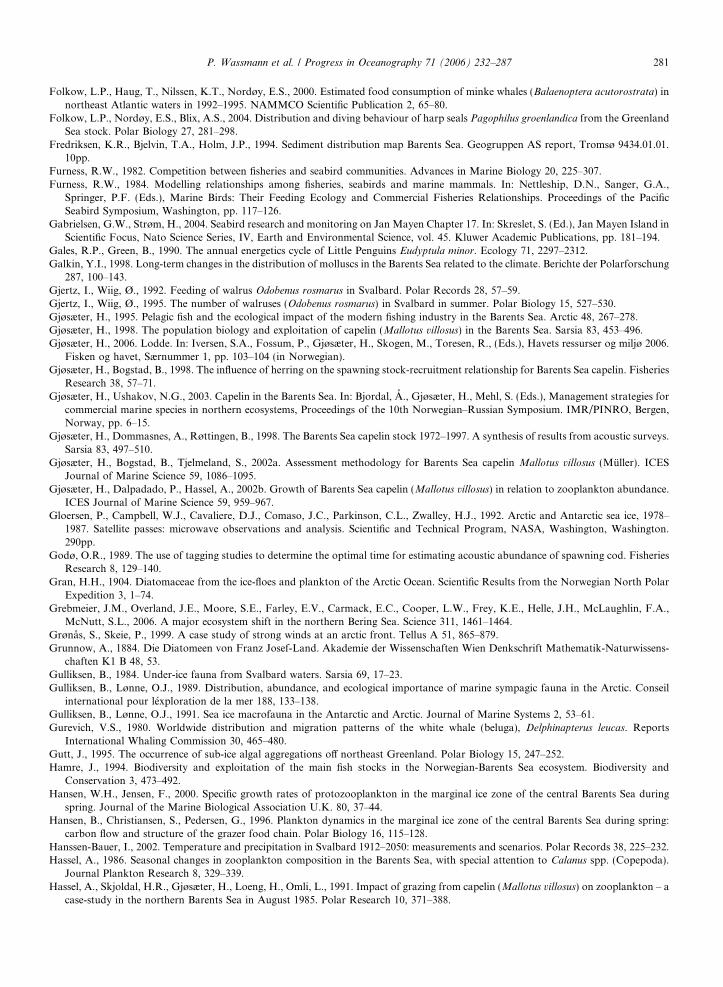
P. Wassmann et al. / Progress in Oceanography 71 (2006) 232–287 281
Folkow, L.P., Haug, T., Nilssen, K.T., Nordøy, E.S., 2000. Estimated food consumption of minke whales (Balaenoptera acutorostrata) innortheast Atlantic waters in 1992–1995. NAMMCO Scientific Publication 2, 65–80.
Folkow, L.P., Nordøy, E.S., Blix, A.S., 2004. Distribution and diving behaviour of harp seals Pagophilus groenlandica from the GreenlandSea stock. Polar Biology 27, 281–298.
Fredriksen, K.R., Bjelvin, T.A., Holm, J.P., 1994. Sediment distribution map Barents Sea. Geogruppen AS report, Tromsø 9434.01.01.10pp.
Furness, R.W., 1982. Competition between fisheries and seabird communities. Advances in Marine Biology 20, 225–307.Furness, R.W., 1984. Modelling relationships among fisheries, seabirds and marine mammals. In: Nettleship, D.N., Sanger, G.A.,
Springer, P.F. (Eds.), Marine Birds: Their Feeding Ecology and Commercial Fisheries Relationships. Proceedings of the PacificSeabird Symposium, Washington, pp. 117–126.
Gabrielsen, G.W., Strøm, H., 2004. Seabird research and monitoring on Jan Mayen Chapter 17. In: Skreslet, S. (Ed.), Jan Mayen Island inScientific Focus, Nato Science Series, IV, Earth and Environmental Science, vol. 45. Kluwer Academic Publications, pp. 181–194.
Gales, R.P., Green, B., 1990. The annual energetics cycle of Little Penguins Eudyptula minor. Ecology 71, 2297–2312.Galkin, Y.I., 1998. Long-term changes in the distribution of molluscs in the Barents Sea related to the climate. Berichte der Polarforschung
287, 100–143.Gjertz, I., Wiig, Ø., 1992. Feeding of walrus Odobenus rosmarus in Svalbard. Polar Records 28, 57–59.Gjertz, I., Wiig, Ø., 1995. The number of walruses (Odobenus rosmarus) in Svalbard in summer. Polar Biology 15, 527–530.Gjøsæter, H., 1995. Pelagic fish and the ecological impact of the modern fishing industry in the Barents Sea. Arctic 48, 267–278.Gjøsæter, H., 1998. The population biology and exploitation of capelin (Mallotus villosus) in the Barents Sea. Sarsia 83, 453–496.Gjøsæter, H., 2006. Lodde. In: Iversen, S.A., Fossum, P., Gjøsæter, H., Skogen, M., Toresen, R., (Eds.), Havets ressurser og miljø 2006.
Fisken og havet, Særnummer 1, pp. 103–104 (in Norwegian).Gjøsæter, H., Bogstad, B., 1998. The influence of herring on the spawning stock-recruitment relationship for Barents Sea capelin. Fisheries
Research 38, 57–71.Gjøsæter, H., Ushakov, N.G., 2003. Capelin in the Barents Sea. In: Bjordal, A., Gjøsæter, H., Mehl, S. (Eds.), Management strategies for
commercial marine species in northern ecosystems, Proceedings of the 10th Norwegian–Russian Symposium. IMR/PINRO, Bergen,Norway, pp. 6–15.
Gjøsæter, H., Dommasnes, A., Røttingen, B., 1998. The Barents Sea capelin stock 1972–1997. A synthesis of results from acoustic surveys.Sarsia 83, 497–510.
Gjøsæter, H., Bogstad, B., Tjelmeland, S., 2002a. Assessment methodology for Barents Sea capelin Mallotus villosus (Muller). ICESJournal of Marine Science 59, 1086–1095.
Gjøsæter, H., Dalpadado, P., Hassel, A., 2002b. Growth of Barents Sea capelin (Mallotus villosus) in relation to zooplankton abundance.ICES Journal of Marine Science 59, 959–967.
Gloersen, P., Campbell, W.J., Cavaliere, D.J., Comaso, J.C., Parkinson, C.L., Zwalley, H.J., 1992. Arctic and Antarctic sea ice, 1978–1987. Satellite passes: microwave observations and analysis. Scientific and Technical Program, NASA, Washington, Washington.290pp.
Godø, O.R., 1989. The use of tagging studies to determine the optimal time for estimating acoustic abundance of spawning cod. FisheriesResearch 8, 129–140.
Gran, H.H., 1904. Diatomaceae from the ice-floes and plankton of the Arctic Ocean. Scientific Results from the Norwegian North PolarExpedition 3, 1–74.
Grebmeier, J.M., Overland, J.E., Moore, S.E., Farley, E.V., Carmack, E.C., Cooper, L.W., Frey, K.E., Helle, J.H., McLaughlin, F.A.,McNutt, S.L., 2006. A major ecosystem shift in the northern Bering Sea. Science 311, 1461–1464.
Grønas, S., Skeie, P., 1999. A case study of strong winds at an arctic front. Tellus A 51, 865–879.Grunnow, A., 1884. Die Diatomeen von Franz Josef-Land. Akademie der Wissenschaften Wien Denkschrift Mathematik-Naturwissens-
chaften K1 B 48, 53.Gulliksen, B., 1984. Under-ice fauna from Svalbard waters. Sarsia 69, 17–23.Gulliksen, B., Lønne, O.J., 1989. Distribution, abundance, and ecological importance of marine sympagic fauna in the Arctic. Conseil
international pour lexploration de la mer 188, 133–138.Gulliksen, B., Lønne, O.J., 1991. Sea ice macrofauna in the Antarctic and Arctic. Journal of Marine Systems 2, 53–61.Gurevich, V.S., 1980. Worldwide distribution and migration patterns of the white whale (beluga), Delphinapterus leucas. Reports
International Whaling Commission 30, 465–480.Gutt, J., 1995. The occurrence of sub-ice algal aggregations off northeast Greenland. Polar Biology 15, 247–252.Hamre, J., 1994. Biodiversity and exploitation of the main fish stocks in the Norwegian-Barents Sea ecosystem. Biodiversity and
Conservation 3, 473–492.Hansen, W.H., Jensen, F., 2000. Specific growth rates of protozooplankton in the marginal ice zone of the central Barents Sea during
spring. Journal of the Marine Biological Association U.K. 80, 37–44.Hansen, B., Christiansen, S., Pedersen, G., 1996. Plankton dynamics in the marginal ice zone of the central Barents Sea during spring:
carbon flow and structure of the grazer food chain. Polar Biology 16, 115–128.Hanssen-Bauer, I., 2002. Temperature and precipitation in Svalbard 1912–2050: measurements and scenarios. Polar Records 38, 225–232.Hassel, A., 1986. Seasonal changes in zooplankton composition in the Barents Sea, with special attention to Calanus spp. (Copepoda).
Journal Plankton Research 8, 329–339.Hassel, A., Skjoldal, H.R., Gjøsæter, H., Loeng, H., Omli, L., 1991. Impact of grazing from capelin (Mallotus villosus) on zooplankton – a
case-study in the northern Barents Sea in August 1985. Polar Research 10, 371–388.
282 P. Wassmann et al. / Progress in Oceanography 71 (2006) 232–287
Haug, T., Svetochev, V., 2004. Seals in the Barents Sea. In: Bjordal, A., Gjøsæter, H., Mehl, S. (Eds.), Management Strategies forCommercial Marine Species in Northern Ecosystems, Proceedings of the 10th Norwegian-Russian Symposium. IMR/PINRO, Bergen,Norway, pp. 131–147.
Haug, T., Nilssen, K.T., Øien, N., Potelov, V., 1994. Seasonal distribution of harp seals (Phoca groenlandica) in the Barents Sea. PolarResearch 13, 161–172.
Haug, T., Lindstrøm, U., Nilssen, K.T., 2002. Variations in minke whale Balaenoptera acutorostrata diet and body condition in responseto ecosystem changes in the Barents Sea. Sarsia 87, 409–422.
Hegseth, E.N., 1992. Sub-ice algal assemblages of the Barents Sea: species composition, chemical composition, and growth rates. PolarBiology 12, 485–496.
Hegseth, E.N., 1998. Primary production of the northern Barents Sea. Polar Research 17, 113–123.Heide-Jørgensen, M.P., 2002. Narwhal Monodon monoceros. In: Perrin, W.F., Wursig, B., Thewissen, J.G.M. (Eds.), Encyclopedia of
Marine Mammals. Academic Press, San Diego, pp. 783–787.Henriksen, G., Gjertz, I., Kondakov, A., 1997. A review of the distribution and abundance of harbour seals, Phoca vitulina, on Svalbard,
Norway, and in the Barents Sea. Marine Mammal Science 13, 157–163.Hirche, H.-J., 1991. Distribution of dominant calanoid copepod species in the Greenland Sea during late fall. Polar Biology 11, 351–
362.Hjelset, A.M., Andersen, M., Gjertz, I., Lydersen, C., Gulliksen, B., 1999. Feeding habits of bearded seals (Erignathus barbatus) from the
Svalbard area, Norway. Polar Biology 21, 186–193.Hop, H., Poltermann, M., Lønne, O.J., Falk-Petersen, S., Korsnes, R., Budgell, W.P., 2000. Ice amphipod distribution relative to ice
density and under-ice topography in the northern Barents Sea. Polar Biology 23, 367.Horner, R.A., 1985. Taxonomy of sea ice microalgae. In: Horner, R.A. (Ed.) Sea ice Biota, Boca Raton, USA, pp. 147–158.Horner, R., Schrader, G.C., 1982. Relative contribution of ice algae, phytoplankton, and benthic microalgae to primary production in
nearshore regions of the Beaufort Sea. Arctic 35, 485–503.Horner, R.A., Syvertsen, E.E., Thomas, D.P., Lange, C., 1988. Proposed terminology and reporting units for sea ice algal assemblages.
Polar Biology 8, 249–253.Howard-Jones, M.H., Ballard, V.D., Allen, A.E., Frischer, M.E., Verity, P.G., 2002. Distribution of bacterial biomass and activity in the
marginal ice zone of the central Barents Sea during summer. Journal of Marine Systems 38, 77–91.Hsiao, S.I.C., 1992. Dynamics of ice algae and phytoplankton in Frobisher Bay. Polar Biology 12, 645–651.Hunt, G.L., Stabeno, P., Walters, G., Sinclair, E., Brodeur, R.D., Napp, J.M., Bond, N.A., 2002. Climate change and cntroll of the
southeastern Bering Strait pelagic ecosystem. Deep Sea Research 49, 5821–5853.Huse, G., 1994. Interactions between herring (Clupea harengus L.) and capelin (Mallotus villosus Muller) in the Barents Sea. Cand. Scient
Thesis, Department of Fisheries and Marine Biology, University of Bergen, 86pp.Huse, G., Toresen, R., 2000. Juvenile herring prey on Barents Sea capelin larvae. Sarsia 85, 385–391.Huse, G., Johansen, G.O., Bogstad, B., Gjøsæter, H., 2004. Studying spatial and trophic interactions between capelin and cod using
individual-based modelling. Journal of Marine Science 61, 1201–1213.ICES, International Council for the Exploration of the Sea, 2004. Report of the Joint ICES/NAFO, Working Group on Harp and
Hooded Seals. International Council for the Exploration of the Sea, Council Meeting 2004/ACFM 6. 40pp.Ilyin, G.V., Matishov, G.G., 1992. Oceanographic conditions in the Pechora Sea in July. In: Matishov, G.G. (Ed.) An International
American–Norwegian–Russian Ecological expedition in the Pechora Sea, Novaya Zemlya, VAYGACH, Kolguyev and Dolgiy Islands,July 1992 (R/V Dalnie Zelentzy). Murmansk Marine Biological Institute, Report, Russian Academy of Sciences, Apatity, Russia, pp7–11 (in Russian).
Ingebrigtsen, A., 1929. Whales caught in the North Atlantic and other seas. Conseil International pour l’exploration de la Mer 56, 1–26.Ingvaldsen, R.B., Asplin, L., Loeng, H., 2004a. Velocity field of the western entrance to the Barents Sea. Journal Geophysical Research
109, C03021. doi:10.1029/2003JC001811.Ingvaldsen, R.B., Asplin, L., Loeng, H., 2004b. The seasonal cycle in the Atlantic transport to the Barents Sea during the years 1997–2001.
Continental Shelf Research 24, 1015–1032.IPCC, 1998. The regional impacts of climate change: an assessment of vulnerability. Cambridge University Press, Cambridge, UK.IPCC, 2001. Climate Change 2001: The Scientific Basis. In: Houghton, J.T., Ding, Y., Griggs, D.J., Noguer, M., van der Linden, P.J.,
Xiaosu, D. (Eds.), Contribution of Working Group I to the Third Assessment Report of the Intergovernmental Panel on ClimateChange. Cambridge University Press, Cambridge, UK.
Jashnov, V.A., 1939. Plankton productivity in the south-western part of the Barents Sea. Trudy VNIRO 4, 201–224 (in Russian).Jashnov, V.A., 1967. Water masses and plankton. I. Species of Calanus finmarchicus as indicator of definite water masses. Zoologichesky
Zhurnal 40, 1314–1334 (in Russian).Jensen, F., Hansen, B.W., 2000. Ciliates and heterotrophic dinoflagellates in the marginal ice zone of the central Barents Sea during spring.
Journal of the Marine Biological Association UK 80, 45–54.Jiang, W., Jørgensen, T., 1996. The diet of haddock (Melanogrammus aeglefinus L.) in the Barents Sea in the period 1984-1991. ICES
Journal Marine Science 53, 11–21.Johannessen, O.M., Bengtsson, L., Miles, M.W., Kuzmina, S.I., Semenov, V.A., Alekseev, G.V., Nagurny, A.P., Zakharov, V.F.,
Bobylev, L.P., Pettersson, L.H., Hasselmann, K., Cattle, H.P., 2002. Arctic climate change – observed and modelled temperature andsea ice. Tellus A 56, 328–341.
Johansen, G.O., 2002. Temporal and spatial variation in predation on juvenile herring (Clupea harengus L.) by northeast Arctic cod(Gadus morhua L.) in the Barents Sea in 1984–1997. ICES Journal Marine Science 59, 270–292.
P. Wassmann et al. / Progress in Oceanography 71 (2006) 232–287 283
Johansen, G.O., 2003. Size-dependent predation on juvenile herring (Clupea harengus L.) by northeast Arctic cod (Gadus morhua L.) in theBarents Sea. Sarsia 88, 136–153.
Johansen, G.O., Bogstad, B., Mehl, S., Ulltang, Ø., 2004. Consumption of juvenile herring (Clupea harengus) by cod (Gadus morhua) in theBarents Sea: a new approach to estimating consumption in piscivorous fish. Canadian Journal of Fisheries and Aquatic Sciences 61,343–359.
Johnsen, G., Hegseth, E.N., 1991. Photoadaptation in marine Arctic diatoms. Polar Biology 9, 479–486.Jonsgard, A., 1966a. The distribution of Balaenopteridae in the North Atlantic Ocean. In: Norris, K.S. (Ed.), Whales, Dolphins and
Porpoises. University of California Press, Berkeley, pp. 114–124.Jonsgard, A., 1966b. Biology of the North Atlantic fin whale Balaenoptera physalus (L.). Taxonomy, distribution, migration and food.
Hvalradets Skrifter 49, 1–62.Karnovsky, N., Kwasniewski, S., Weslawski, J.M., Walkusz, W., Beszczynska-Møller, A., 2003. The foraging behavior of little auks in a
heterogeneous environment. Marine Ecology Progress Series 253, 289–303.Kendall, M.A., 1996. Are Arctic soft sediment macrobenthic communities impoverished? Polar Biology 16, 393–399.Klages, M., Boetius, A., Christensen, J.P., Deubel, H., Piepenburg, D., Schewe, I., Soltwedel, T., 2004. The benthos of Arctic Seas and its
role for the organic carbon cycle at the seafloor. In: Stein, R., Macdonald, R.W. (Eds.), The Organic Carbon Cycle in the Arctic Ocean.Springer, Berlin–Heidelberg, pp. 139–167.
Kuznetsov, A.P., 1970. Features of the bottom invertebrate trophic group distribution in the Barents Sea. Transactions of the Institute forOceanology 88, 5–80.
Kuznetsov, L.L., Schoschina, E.V., 2003. Phytocenoses of the Barents Sea (Physiological and Structural Characteristics). Kola ScientificCentre RAS, Apatity, Russia, 308p. (in Russian).
Lavigne, D.M., Kovacs, K.M., 1988. Harps and HoodsIce-breeding Seals of the Northwest Atlantic. University of Waterloo Press,Waterloo, Ontario.
Lee, R.F., 1975. Lipids of zooplankton. Comparative Biochemical Physiology B 51, 263–266.Legendre, L., Ackley, S.F., Dieckmann, G.S., Gulliksen, B., Horner, R., Hoshiai, T., Melnikov, I.A., Reeburgh, W.S., Spindler, M.,
Sullivan, C.W., 1992. Ecology of sea ice biota. 2. Global significance. Polar Biology 12, 429–444.Li, S., 1995. The dynamics of a slope current in the Barents Sea. Dr. Ing. thesis, University of Trondheim. 141pp.Lindstrøm, U., Harbitz, A., Haug, T., Nilssen, K.T., 1998. Do harp seals Phoca groenlandica exhibit particular prey preferences? ICES
Journal of Marine Science 55, 941–953.Lindstrøm, U., Haug, T., Røttingen, I., 2002. Predation on herring (Clupea harengus) by minke whales (Balaenoptera acutorostrata) in the
Barents Sea. ICES Journal of Marine Science 59, 58–70.Linko, A.K., 1907. Investigation of the composition and life of plankton in the Barents Sea. St. Petersburg, p. 247 (in Russian).Loeng, H., 1991. Features of the physical oceanographic conditions in the central parts of the Barents Sea. Polar Research 10, 5–18.Loeng, H., 1992. Fysisk Oseanografi. In: Sakshaug, E. (Ed.) Økosystem Barentshavet, NAVF, NFFR, MD, Oslo, pp. 23–42 (in
Norwegian).Loeng, H., Sætre, R., 2001. Features of the Barents Sea circulation. Fisken og Havet 1-2001, 40.Loeng, H., Ozhigin, V., Adlandsvik, B., Sagen, H., 1993. Current Measurements in the northeastern Barents Sea. International Council
for the Exploration of the Sea, Council Meeting 1993/C:41, Hydrographic Committee, 22pp.Loeng, H., Ozhigin, V., Adlandsvik, B., 1997. Water fluxes through the Barents Sea. ICES Journal of Marine Science 54, 310–317.Lønne, O.J., Gabrielsen, G.W., 1992. Summer diet of seabirds feeding in sea-ice-covered waters near Svalbard. Polar Biology 12, 685–
692.Lønne, O.J., Gulliksen, B., 1989. Size, age and diet of polar cod, Boreogadus saida (Lepechin 1773), in ice covered waters. Polar Biology 9,
187–191.Lønne, O.J., Gulliksen, B., 1991a. On the distribution of sympagic macro-fauna in the seasonally ice covered Barents Sea. Polar Biology
11, 457–469.Lønne, O.J., Gulliksen, B., 1991b. Source, density and composition of sympagic fauna in the Barents Sea. Polar Research 10, 289–294.Lønne, O.J., Gulliksen, B., 1991c. Sympagic macro-fauna from mulityear sea-ice near Svalbard. Polar Biology 11, 471–477.Lopez, P., Schmith, T., Kaas, E., 2000. Sensitivity of the Northern Hemisphere circulation to North Atlantic SSTs in the ARPEGE
Climate AGCM. Climate Dynamics 16, 535–547.Lydersen, C., 1998. Status and biology of ringed seals (Phoca hispida) in Svalbard. NAMMCO Science Publications 1, 46–62.Lydersen, C., Martin, A.R., Kovacs, K.M., Gjertz, I., 2001. Summer and autumn movements of white whales Delphinapterus leucas in
Svalbard, Norway. Marine Ecology Progress Series 219, 265–274.Makarevich, P.R., Larionov, V.V., 1992. Taxonomical composition of phytoplankton and history of the phytoplankton studies in the
Barents Sea. In: Phytoplankton of the Barents Sea, Apatity, Russia, pp. 17–51.Matrai, P., Vernet, M., Wassmann, P., 2006. Sulfur and carbon relationships in Arctic phytoplankton: influence of time and space scales.
Journal of Marine Systems, submitted, doi:10.1016/j.jmarsys.2006.10.001.Maykut, G.A., 1985. The ice environment. In: Horner, R.A. (Ed.), Sea Ice Biota. CRC Press, Boca Raton, USA, pp. 21–82.McMahon, K.W., Ambrose, W.G., Johnson, B.J., Sun, M., Lopez, G.R., Clough, L.M., Carroll, M.L., 2006. Benthic community response
to ice algae and phytoplankton in Ny Alesund, Svalbard. Marine Ecology Progress Series 310, 1–14.McMinn, A., Hegseth, E.N., 2004. Quantum yield and photosynthetic parameters of marine microalga from the southern Arctic Ocean,
Svalbard. Journal of the Marine Biological Association UK 84, 865–871.Mehl, S., 1989. The northeast Arctic cod stock’s consumption of commercially exploited prey species in 1984–1986. Conseil International
pour l’exploration de la Mer 188, 185–205.
284 P. Wassmann et al. / Progress in Oceanography 71 (2006) 232–287
Mehl, S., Sunnana, K., 1991. Changes in growth of Northeast Arctic cod in relation to food consumption in 1984–1988. ICES MarineScience Symposium 193, 109–112.
Mehl, S., Yaragina, N.A., 1992. Methods and results in the joint PINRO-IMR stomach sampling program. In: Bogstad, B., Tjelmeland, S.(Eds.), Interrelations between Fish Populations in the Barents Sea, Proceedings of the 5th PINRO-IMR Symposium. IMR-PINRO,Bergen, Norway, pp. 5–16.
Mehlum, F., Gabrielsen, G.W., 1993. The diet of high arctic seabirds in coastal and ice-covered, pelagic areas near the Svalbardarchipelago. Polar Research 11, 1–20.
Mehlum, F., Gabrielsen, G.W., 1995. Energy expenditure and food consumption by seabird populations in the Barents Sea region. In:Skjoldal, H.R., Hopkins, C., Erikstad, K.E., Leinaas, H.P. (Eds.), Ecology of Fjords and Coastal Waters. Elsevier Science,Amsterdam, pp. 457–470.
Mei, Z.-P., Legendre, L., Gratton, Y., Tremblay, J.E., LeBlanc, B., Klein, B., Gosselin, M., 2003. Phytoplankton production in the NorthWater Polynya: size-fractions and carbon fluxes, April to July 1998. Marine Ecology Progress Series 256, 13–27.
Melle, W., Skjoldal, H.R., 1998. Reproduction and development of Calanus finmarchicus, C. glacialis andC. hyperboreus in the BarentsSea. Marine Ecology Progress Series 169, 211–228.
Melnikov, I., 1997. The Arctic Sea Ice System. Gordon and Breach Science Publishers, Amsterdam, 204pp.Michalsen, K. (Ed.) 2004. Havets Ressurser 2004. Fisken og Havet, Special edition, 1-2004, 178pp.Michalsen, K., Nedreaas, K.H., 1998. Food and feeding of Greenland halibut (Reinhardtius hippoglossoides, Wilbaum) in the Barents Sea
and East-Greenland waters. Sarsia 83, 401–407.Midttun, L., 1985. Formation of dense bottom water in the Barents Sea. Deep-Sea Research 32, 1233–1241.Millimann, J.D., Syvitski, J.P.M., 2002. Geomorphic/tectonic control of sediment discharge to the oceans: the importance of small
mountainous rivers. Journal of Geology 100, 525–544.Misund, O.A., Melle, W., Ferno, A., 1997. Migration behaviour of Norwegian spring spawning herring when entering the cold front in the
Norwegian Sea. Sarsia 82, 107–112.NAMMCO, 1998. North Atlantic Marine Mammal Commission. 1998. Report of the 5th Meeting of the Scientific Committee. In:
NAMMCO Annual Report 1997, NAMMCO, Tromsø, Norway, pp. 85–202.NAMMCO, 2003. North Atlantic Marine Mammal Commission. 2003. Report of the 11th Meeting of the Scientific Committee. In:
NAMMCO Annual Report 2003, NAMMCO, Tromsø, Norway, pp 135–310.Nansen, F., 1906. Northern waters, Captain Roald Amundsen’s oceanographic observations in the Arctic Seas in 1901. Videnskab-
Selskabets Skrifter 1, Matematisk-Naturvidenskabelig Klasse 1, Kristiania, pp. 1–145.Nikiforov, E.G., Shpaiker, A.O., 1980. Principles of large-scale variations of the Arctic Ocean hydrography. Hydrometeizdat, Leningrad,
269pp. (in Russian).Nilssen, K.T., Haug, T., 2007. Status of grey seals (Halichoerus grypus) in Norway. NAMMCO Scientific Publications, 5 (in press).Nilssen, K.T., Haug, T., Potelov, V., Timoshenko, Y.K., 1995a. Food habits and food availability of harp seals (Phoca groenlandica)
during early summer and autumn in the northern Barents Sea. Polar Biology 15, 485–493.Nilssen, K.T., Haug, T., Potelov, V., Stasenkov, V.A., Timoshenko, Y.K., 1995b. Food habits of harp seals (Phoca groenlandica)
during lactation and moult in March–May in the southern Barents Sea and White Sea. ICES Journal of Marine Science 52, 33–41.
Nilssen, K.T., Pedersen, O.-P., Folkow, L., Haug, T., 2000. Food consumption estimates of Barents Sea harp seals. NAMMCO SciencePublication 2, 9–28.
Nilssen, K.T., Haug, T., Corkeron, P., Lindblom, L., 2001. On the diet of grey seals, Halichoerus grypus, in Lofoten and Finnmark, NorthNorway. ICES Working Group on Marine Mammals Population Dynamics, Copenhagen, Denmark, 23–27 April, 15pp.
Norrbin, M.F., 1991. Gonad maturation as an indication of seasonal cycles for several species of small copepods in the Barents Sea. PolarResearch 10, 205–211.
Nøttestad, L., Ferno, A., Mackinson, S., Pitcher, T., Misund, O.A., 2002. How whales influence herring school dynamics in a cold-frontarea of the Norwegian Sea. ICES Journal of Marine Science 59, 393–400.
O’Corry-Crowe, G.M., 2002. Beluga whale Delphinapterus leucas. In: Perrin, W.F., Wursig, B., Thewissen, J.G.M. (Eds.), Encyclopedia ofMarine Mammals. Academic Press, San Diego, pp. 94–99.
Øien, N., 1993. A note on Lagenorhynchus species in Norwegian waters. ICES Study Group on Seals and Small Cetaceans in EuropeanSeas, Cambridge, 31 March–2 April. Working paper, 9pp.
Olli, K., Wexels Riser, C., Wassmann, P., Ratkova, T.N., Arashkevich, E., Pasternak, A., 2002. Seasonal variation in vertical flux ofbiogenic matter in the marginal ice zone and the central Barents Sea. Journal of Marine Systems 38, 189–204.
Olsen, A., Johannessen, T., Rey, F., 2003. On the nature of the factors that control spring bloom development at the entrance to theBarents Sea and their interannual variability. Sarsia 88, 379–393.
Ottersen, G., Adlandsvik, B., Loeng, H., 2000. Predicting the temperature of the Barents Sea. Fisheries Oceanography 9, 121–135.Pasternak, A., Arashkevich, E., Wexels Riser, C., Reigstad, M., Wassmann, P., 2002. Calanus spp. grazing affects egg production and
vertical carbon flux in the marginal ice zone and open Barents Sea. Journal of Marine Systems 38, 147–163.Pavlov, V., Pavlova, O., Korsnes, R., 2004. Sea ice fluxes and drift trajectories from potential pollution sources, computed with a statistical
sea ice model of the Arctic Ocean. Journal of Marine Systems 48, 133–157.Pedersen, G., 1995. Factors influencing the size and distribution of the copepod community in the Barents Sea with special emphasis on
Calanus finmarchicus (Gunnerus). Dr. Scient. Thesis, Norwegian College of Fishery Science, University of Tromsø.Pedersen, G., Tande, K.S., Nilssen, E.M., 1995. Temporal and regional variation in the copepod community in the central Barents Sea
during spring and early summer 1988 and 1989. Journal of Plankton Research 17, 263–282.
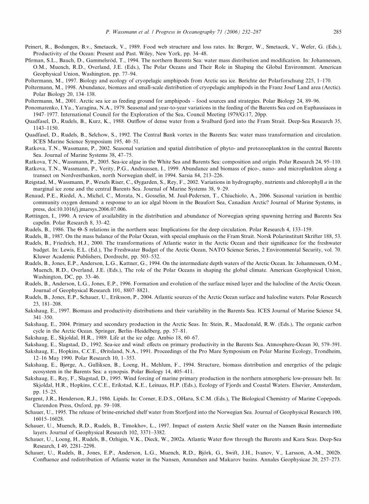
P. Wassmann et al. / Progress in Oceanography 71 (2006) 232–287 285
Peinert, R., Bodungen, B.v., Smetacek, V., 1989. Food web structure and loss rates. In: Berger, W., Smetacek, V., Wefer, G. (Eds.),Productivity of the Ocean: Present and Past. Wiley, New York, pp. 34–48.
Pfirman, S.L., Bauch, D., Gammelsrod, T., 1994. The northern Barents Sea: water mass distribution and modification. In: Johannessen,O.M., Muench, R.D., Overland, J.E. (Eds.), The Polar Oceans and Their Role in Shaping the Global Environment. AmericanGeophysical Union, Washington, pp. 77–94.
Poltermann, M., 1997. Biology and ecology of cryopelagic amphipods from Arctic sea ice. Berichte der Polarforschung 225, 1–170.Poltermann, M., 1998. Abundance, biomass and small-scale distribution of cryopelagic amphipods in the Franz Josef Land area (Arctic).
Polar Biology 20, 134–138.Poltermann, M., 2001. Arctic sea ice as feeding ground for amphipods – food sources and strategies. Polar Biology 24, 89–96.Ponomarenko, I.Ya., Yaragina, N.A., 1979. Seasonal and year-to-year variations in the feeding of the Barents Sea cod on Euphausiacea in
1947–1977. International Council for the Exploration of the Sea, Council Meeting 1979/G:17, 20pp.Quadfasel, D., Rudels, B., Kurz, K., 1988. Outflow of dense water from a Svalbard fjord into the Fram Strait. Deep-Sea Research 35,
1143–1150.Quadfasel, D., Rudels, B., Selchow, S., 1992. The Central Bank vortex in the Barents Sea: water mass transformation and circulation.
ICES Marine Science Symposium 195, 40–51.Ratkova, T.N., Wassmann, P., 2002. Seasonal variation and spatial distribution of phyto- and protozooplankton in the central Barents
Sea. Journal of Marine Systems 38, 47–75.Ratkova, T.N., Wassmann, P., 2005. Sea-ice algae in the White Sea and Barents Sea: composition and origin. Polar Research 24, 95–110.Ratkova, T.N., Wassmann, P., Verity, P.G., Andreassen, I., 1999. Abundance and biomass of pico-, nano- and microplankton along a
transect on Nordvestbanken, north Norwegian shelf, in 1994. Sarsia 84, 213–226.Reigstad, M., Wassmann, P., Wexels Riser, C., Øygarden, S., Rey, F., 2002. Variations in hydrography, nutrients and chlorophyll a in the
marginal ice zone and the central Barents Sea. Journal of Marine Systems 38, 9–29.Renaud, P.E., Riedel, A., Michel, C., Morata, N., Gosselin, M. Juul-Pedersen, T., Chiuchiolo, A., 2006. Seasonal variation in benthic
community oxygen demand: a response to an ice algal bloom in the Beaufort Sea, Canadian Arctic? Journal of Marine Systems, inpress, doi:10.1016/j.jmarsys.2006.07.006.
Røttingen, I., 1990. A review of availability in the distribution and abundance of Norwegian spring spawning herring and Barents Seacapelin. Polar Research 8, 33–42.
Rudels, B., 1986. The H–S relations in the northern seas: Implications for the deep circulation. Polar Research 4, 133–159.Rudels, B., 1987. On the mass balance of the Polar Ocean, with special emphasis on the Fram Strait. Norsk Polarinstitutt Skrifter 188, 53.Rudels, B., Friedrich, H.J., 2000. The transformations of Atlantic water in the Arctic Ocean and their significance for the freshwater
budget. In: Lewis, E.L. (Ed.), The Freshwater Budget of the Arctic Ocean, NATO Science Series, 2 Environmental Security, vol. 70.Kluwer Academic Publishers, Dordrecht, pp. 503–532.
Rudels, B., Jones, E.P., Anderson, L.G., Kattner, G., 1994. On the intermediate depth waters of the Arctic Ocean. In: Johannessen, O.M.,Muench, R.D., Overland, J.E. (Eds.), The role of the Polar Oceans in shaping the global climate. American Geophysical Union,Washington, DC, pp. 33–46.
Rudels, B., Anderson, L.G., Jones, E.P., 1996. Formation and evolution of the surface mixed layer and the halocline of the Arctic Ocean.Journal of Geophysical Research 101, 8807–8821.
Rudels, B., Jones, E.P., Schauer, U., Eriksson, P., 2004. Atlantic sources of the Arctic Ocean surface and halocline waters. Polar Research23, 181–208.
Sakshaug, E., 1997. Biomass and productivity distributions and their variability in the Barents Sea. ICES Journal of Marine Science 54,341–350.
Sakshaug, E., 2004. Primary and secondary production in the Arctic Seas. In: Stein, R., Macdonald, R.W. (Eds.), The organic carboncycle in the Arctic Ocean. Springer, Berlin–Heidelberg, pp. 57–81.
Sakshaug, E., Skjoldal, H.R., 1989. Life at the ice edge. Ambio 18, 60–67.Sakshaug, E., Slagstad, D., 1992. Sea-ice and wind: effects on primary productivity in the Barents Sea. Atmosphere-Ocean 30, 579–591.Sakshaug, E., Hopkins, C.C.E., Øritsland, N.A., 1991. Proceedings of the Pro Mare Symposium on Polar Marine Ecology, Trondheim,
12–16 May 1990. Polar Research 10, 1–353.Sakshaug, E., Bjørge, A., Gulliksen, B., Loeng, H., Mehlum, F., 1994. Structure, biomass distribution and energetics of the pelagic
ecosystem in the Barents Sea: a synopsis. Polar Biology 14, 405–411.Sakshaug, E., Rey, F., Slagstad, D., 1995. Wind forcing of marine primary production in the northern atmospheric low-pressure belt. In:
Skjoldal, H.R., Hopkins, C.C.E., Erikstad, K.E., Leinaas, H.P. (Eds.), Ecology of Fjords and Coastal Waters. Elsevier, Amsterdam,pp. 15–25.
Sargent, J.R., Henderson, R.J., 1986. Lipids. In: Corner, E.D.S., OHara, S.C.M. (Eds.), The Biological Chemistry of Marine Copepods.Clarendon Press, Oxford, pp. 59–108.
Schauer, U., 1995. The release of brine-enriched shelf water from Storfjord into the Norwegian Sea. Journal of Geophysical Research 100,16015–16028.
Schauer, U., Muench, R.D., Rudels, B., Timokhov, L., 1997. Impact of eastern Arctic Shelf water on the Nansen Basin intermediatelayers. Journal of Geophysical Research 102, 3371–3382.
Schauer, U., Loeng, H., Rudels, B., Ozhigin, V.K., Dieck, W., 2002a. Atlantic Water flow through the Barents and Kara Seas. Deep-SeaResearch, I 49, 2281–2298.
Schauer, U., Rudels, B., Jones, E.P., Anderson, L.G., Muench, R.D., Bjork, G., Swift, J.H., Ivanov, V., Larsson, A.-M., 2002b.Confluence and redistribution of Atlantic water in the Nansen, Amundsen and Makarov basins. Annales Geophysicae 20, 257–273.
286 P. Wassmann et al. / Progress in Oceanography 71 (2006) 232–287
Scott, C., Falk-Petersen, S., Hop, H., Sargent, J.R., Lønne, O.J., Poltermann, M., 1999. Lipids and trophic interaction of ice fauna andpelagic zooplankton in the Marginal Ice Zone of the Barents Sea. Polar Biology 21, 65–70.
Sendstad, E., 1977. Notes on the biology of the Arctic bird rock. Norsk Polarinstitutt Arbok 1977/78, 265–270.Sergeant, D.E., 1991. Harp seal, man and ice. Canadian Journal of Fisheries and Aquatic Sciences Special Publication 114, 153.Simila, T., Holst, J.C., Christensen, I., 1996. Occurrence and diet of killer whales in northern Norway: seasonal patterns relative to the
distribution and abundance of Norwegian spring spawning herring. Canadian Journal of Fisheries and Aquatic Sciences 53, 769–779.Sirenko, B.S., 2001. List of species of free living invertebrates of Eurasian Arctic Seas and adjacent deep waters. In: Explorations of the
Fauna of the Seas 51 (59). Russian Academy of Sciences, St. Petersburg, Russia.Skaug, H.J., Øien, N., Schweder, T., Bøthun, G., 2004. Abundance of minke whales (Balenoptera acutorostrata) in the northeast Atlantic:
variability in time and space. Canadian Journal Of Fisheries and Aquatic Sciences 61, 870–886.Skeie, K., 1995. Choice of food and partitioning of niches among seal species in Jarfjord, Finnmark. Cand. scient. Thesis, Biological
Institute, University of Oslo, Norway, 60pp. (in Norwegian).Skjoldal, H.R., Rey, F., 1989. pelagic production and variability of the Barents Sea ecosystem. In: Sherman, K., Alexander, L.M. (Eds.),
Biomass yields and geography of large marine ecosystems, AAAS Selected Symposium, vol. 111. Westview Press, pp. 241–286.Skjoldal, H.R., Hassel, A., Rey, F., 1987. Spring phytoplankton development and zooplankton reproduction in the central Barents
Sea in the period 1979-1984. In: Loeng, H. (Ed.), The effect of oceanographic conditions on distribution and population dynamicsof commercial fish stocks in the Barents Sea, Proceedings of the 3rd Soviet–Norwegian Symposium. IMR/PINRO, Bergen, pp.59–89.
Skjoldal, H.R., Gjøsæter, H., Loeng, H., 1992. The Barents Sea ecosystem in the 1980s: ocean cimate, plankton and capelin growth. ICESMarine Science Symposia 195, 278–290.
Slagstad, D., McClimans, T., 2005. Modelling the ecosystem dynamics of the marginal ice zone and central Barents Sea. I. Physical andchemical oceanography. Journal of Marine Systems 58, 1–18.
Slagstad, D., Stokke, S., 1984. Simulations of currents, hydrography, and ice distribution and primary production in the northern sector ofthe Barents Sea. Fish and Sea (Institute of Marine Research) 9, 1–47 (in Norwegian).
Slagstad, D., Wassmann, P., 1997. Climate change and carbon flux in the Barents Sea: 3-D simulations of ice-distribution, primaryproduction and vertical export of particulate organic matter. National Institute of Polar Research, Special Issue, 51, pp. 119–141.
Smetacek, V., 1985. Role of sinking in diatom life-history cycles: ecological, evolutionary, and geological significance. Marine Biology 84,239–251.
Smith, S.L., 1990. Egg production and feeding by copepods prior to the spring bloom of phytoplankton in Fram Strait, Greenland Sea.Marine Biology 106, 59–69.
Smith, T.D., Allen, J., Clapham, P.J., Hammond, P.S., Katona, S., Larsen, F., Lien, J., Mattila, D., Palsbøll, P.J., Sigurjonsson, J.,Stevick, P.T., Øien, N., 1999. An ocean-basin-wide mark-recapture study of the North Atlantic humpback whale (Megaptera
novaeangliae). Marine Mammal Science 15, 1–32.Søreide, J.E., Hop, H., Falk-Petersen, S., Gulliksen, B., Hansen, E., 2003. Macrozooplankton communities and environmental variables in
the Barents Sea marginal ice zone in late winter and spring. Marine Ecology Progress Series 263, 43–64.Stabeno, P.J., Overland, J.E., 2001. Bering Sea shifts toward an earlier spring transition. EOS 82, 317–321.Strass, V.H., Nothig, E.-M., 1996. Seasonal shifts in the ice edge phytoplankton blooms in the Barents Sea related to the water column
stability. Polar Biology 16, 409–422.Sturlusson, M., 2005. Implementing the microbial food web in the Barents Sea pelagic ecosystem. Master of Science Thesis, University of
Copenhagen.Syvertsen, E.E., 1991. Ice algae in the Barents Sea: types of assemblages, origin, fate and role in the ice edge phytoplankton bloom. Polar
Research 10, 277–287.Tamelander, T., Renaud, P.E., Hop, H., Carroll, M.L., Ambrose Jr., W.G., Hobson, K.A., 2005. Trophic relationships and pelagic–
benthic coupling during summer in the Barents Sea Marginal Ice Zone revealed by stable carbon and nitrogen isotope measurements.Marine Ecology Progress Series 310, 33–46.
Tande, K.S., 1991. Calanus in North Norwegian fjords and in the Barents Sea. Polar Research 10, 389–407.Tantsiura, A.I., 1959. On the currents of the Barents Sea. Transactions of the Polar Scientific Research Institute of Marine Fisheries and
Oceanography (PINRO) 11, 35–53 (in Russian).Thingstad, T.F., Martinussen, I., 1991. Are bacteria active in the cold pelagic ecosystem of the Barents Sea? Polar Research 10, 255–267.Timofeev, S.F., 1997. Zooplankton in the Barents Sea. In: Matishov, G.G. (Ed.) Plankton of the Sea of the Western Arctic. Apatity,
Russia, pp. 266–295.Timoshenko, Y.K., Popov, L.A., 1990. On the predatory habits of the Atlantic walrus. In: Fay, F.H., Kelly, B.P., Fay, B.A. (Eds.), The
ecology and management of walrus populations. Report of an International Workshop, Marine Mammal Commission Report FB91-100479, pp. 177–178.
Usachev, P.T., 1949. The microflora of polar ice. Trudy Instituta Okeanologii Akademii Nauk SSSR 3, 216–259 (in Russian).Verity, P., Wassmann, P., Ratkova, T.N., Andreassen, I.J., 1999. Seasonal patterns in composition and biomass of autotrophic and
heterotrophic microplankton communities on the north Norwegian shelf. Sarsia 84, 265–278.Verity, P.G., Wassmann, P., Frischer, M.E., Howard-Jones, M.H., Allen, A.E., 2002. Grazing of primary production by
microzooplankton in the Barents Sea during early summer. Journal of Marine Systems 38, 109–123.Vernet, M., Matrai, P.A., Andreassen, I.J., 1998. Synthesis of particulate and extracellular carbon by phytoplankton at the marginal ice-
zone in the Barents Sea. Journal of Geophysical Research on Continental Oceans 103, 1023–1037.Vetrov, A.A., Romankevich, E.A., 2004. Carbon cycle in the Russian Arctic. Springer, Berlin–Heidelberg, 331pp.
P. Wassmann et al. / Progress in Oceanography 71 (2006) 232–287 287
Vinje, T., 1985. Drift, composition, morphology and distribution of the sea ice fields in the Barents Sea. Norsk Polarinstitutt Skrifter C197, 1–26.
Vinje, T., 2001. Anomalies and trends of sea ice extent and atmospheric circulation in the Nordic Seas during the period 1864-1998.Journal of Climatology 14, 255–267.
Vinje, T.R., Goosse, H., 2004. Ice extent variations during last centuries. In: Poster in Proceedings of the ACSYS Final ScienceConference, St Petersburg, Russia, 11–14 November 2003. WCRP – 118 (CD); World Meteorological Organization. TD No 1232.
Vinje, T., Kvambek, A.S., 1991. Barents Sea drift ice characteristics. Polar Research 10, 59–68.von Quillfeldt, C.H., 2000. Common diatoms species in Arctic spring blooms: their distribution and abundance. Botanica Marina 43, 499–
516.Walsh, J.J., Sakshaug, E., 2000. Marine biology: biomass, productivity, distribution and their variability in the Barents Sea. In: Nuttal,
M., Callaghan, T.V. (Eds.), The Arctic: Environment, People, Policy. Harwood, Amsterdam, pp. 163–196.Wassmann, P., 1989. Sedimentation of organic matter and silicate from the euphotic zone of the Barents Sea. Rapports Conseil
international pour lexploration de la Mer 188, 108–114.Wassmann, P., 1990. Relation between primary and export production in the boreal coastal zone of the North Atlantic. Limnology and
Oceanography 35, 464–471.Wassmann, P., 1998. Retention versus export food chains: processes controlling sinking loss from marine pelagic systems. Hydrobiologia
363, 29–57.Wassmann, P., 2001. Vernal export and retention of biogenic matter in the north-eastern North Atlantic and adjacent Arctic Ocean: the
role of the Norwegian Atlantic Current and topography. National Institute of Polar Research, Special Issue, 54, pp. 377–392.Wassmann, P., 2002. Seasonal C-cycling variability in the open and ice-covered waters of the Barents Sea: an introduction. Journal of
Marine Systems 38, 1–7.Wassmann, P., Slagstad, D., 1993. Seasonal and interannual dynamics of carbon flux in the Barents Sea: a model approach. Polar Biology
13, 363–372.Wassmann, P., Martinez, R., Vernet, M., 1993. Respiration and biochemical composition of sedimenting organic matter during summer in
the Barents Sea. Continental Shelf Research 14, 79–90.Wassmann, P., Ratkova, T.N., Andreassen, I., Vernet, M., Pedersen, G., Rey, F., 1999a. Spring bloom development in the marginal ice
zone and the central Barents Sea. Marine Ecology 20, 321–346.Wassmann, P., Andreassen, I., Rey, F., 1999b. Seasonal variation of nutrients and suspended biomass along a transect on
Nordvestbanken, north Norwegian shelf, in 1994. Sarsia 84, 199–212.Wassmann, P., Olli, K., Wexels Riser, C., Svensen, C., 2003. Ecosystem function, biodiversity and vertical flux regulation in the twilight
zone. In: Wefer, G., Lamy, F., Mantoura, F. (Eds.), Marine Science Frontiers for Europe. Springer, Heidelberg–Berlin–New York, pp.279–287.
Wassmann, P., Bauernfeind, E., Fortier, M., Fukuchi, M., Hargrave, B., Moran, B., Noji, T., Nothig, E.-M., Peinert, R., Sasaki, H.,Shevchenko, V., 2004. Particulate organic carbon flux to the sea floor. In: Stein, R., Macdonald, R.M. (Eds.), The Organic CarbonCycle in the Arctic Ocean. Springer, Heidelberg–Berlin–New York, pp. 101–138.
Wassmann, P., Ratkova, T., Reigstad, M., 2005. The contribution of solitary and colonial cells of Phaeocystis pouchetii to spring andsummer blooms in the north-eastern North Atlantic. Harmful Algae 4, 823–840.
Wassmann, P., Slagstad, D., Wexels Riser, C., Reigstad, M., 2006. Modelling the ecosystem dynamics of the marginal ice zone and centralBarents Sea. II. Carbon flux and interannual variability. Journal of Marine Systems 59, 1–24.
Wathne, J.A., Haug, T., Lydersen, C., 2000. Prey preference and niche overlap of ringed seals Phoca hispida and harp seals P. groenlandica
in the Barents Sea. Marine Ecology Progress Series 194, 233–239.Weller, G., Lange, M., 1999. Impacts of Global Climate Change in the Arctic regionsAn Initial Assessment. International Arctic Science
Committee (IASC), Oslo, Norway.Werner, I., 1997. Grazing of Arctic under-ice amphipods on sea ice algae. Marine Ecology Progress Series 160, 93–99.Werner, I., Auel, H., Garrity, C., Hagen, W., 1999. Pelagic occurrence of the sympagic amphipod Gammarus wilkitzkii in ice free waters of
the Greenland Sea - dead end or part of life cycle? Polar Biology 22, 56–60.Wexels Riser, C., Wassmann, P., Olli, K., Pasternak, A., Arashkevich, E., 2002. Seasonal variation in production, retention and export of
zooplankton faecal pellets in the marginal ice zone and the central Barents Sea. Journal of Marine Systems 38, 175–188.Zelikman, E.A., Golovkin, A.N., 1972. Composition, structure and productivity of neritic communities near the bird colonies of the
northern shores of Novaya Zemlya. Marine Biology 17, 265–274.Zelikman, E.A., Kamshilov, M.M., 1960. The long-term dynamics of plankton biomass in the southern part of the Barents Sea, and
factors influencing it. Trudy Murmansk Marine Biological Institute 2, 68–113 (in Russian).Zenkevich, L.A., 1963. Biology of the Seas of the USSR. George Allen and Unwin Ltd, London.