flux and divergence

Chapter 13

Flux and Divergence

A vector field is a function with direction, and because of this directionalproperty, many new kinds of differentiation and integration can be performedon it. For instance, a vector field can be made to pierce a surface or an elementthereof, and as it pierces that surface its variation from point to point can bemonitored. This leads to one kind of differentiation and integration which wediscuss next. The integration leads to the concept of the flux of a vector field,and the associated differentiation to the notion of divergence.

13.1 Flux of a Vector Field

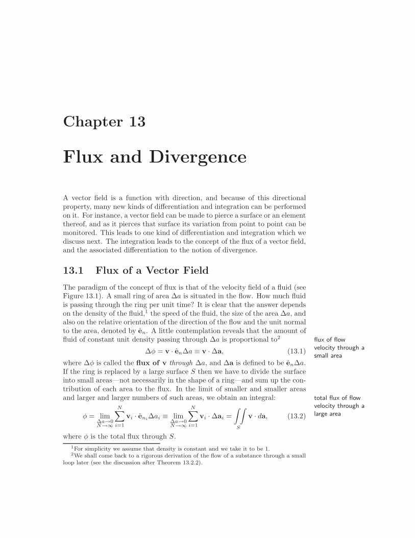
The paradigm of the concept of flux is that of the velocity field of a fluid (seeFigure 13.1). A small ring of area ∆a is situated in the flow. How much fluidis passing through the ring per unit time? It is clear that the answer dependson the density of the fluid,1 the speed of the fluid, the size of the area ∆a, andalso on the relative orientation of the direction of the flow and the unit normalto the area, denoted by en. A little contemplation reveals that the amount offluid of constant unit density passing through ∆a is proportional to2 flux of flow

velocity through asmall area

∆φ = v · en∆a ≡ v · ∆a, (13.1)

where ∆φ is called the flux of v through ∆a, and ∆a is defined to be en∆a.If the ring is replaced by a large surface S then we have to divide the surfaceinto small areas—not necessarily in the shape of a ring—and sum up the con-tribution of each area to the flux. In the limit of smaller and smaller areasand larger and larger numbers of such areas, we obtain an integral: total flux of flow

velocity through alarge areaφ = lim

∆a→0N→∞

N!

i=1

vi · eni∆ai ≡ lim∆a→0N→∞

N!

i=1

vi · ∆ai =" "

S

v · da, (13.2)

where φ is the total flux through S.1For simplicity we assume that density is constant and we take it to be 1.2We shall come back to a rigorous derivation of the flow of a substance through a small

loop later (see the discussion after Theorem 13.2.2).

366 Flux and Divergence

ˆ e n

vda

Figure 13.1: Flux of velocity vector through a small area ∆a.

There is an arbitrariness in the direction of the unit vector normal to anelement of area, because for any unit normal, there is another which points inthe opposite direction. The flux for these two unit normals will have oppositesigns. This may appear as if one could arbitrarily choose every one of theunit normals eni in the sum (13.2) to have either one of the two oppositeorientations, leading to an arbitrary result for the integral. This is not the case,the total flux can

be determinedonly up to a sign.

because the direction of the unit normal to an element of area is determinedby the neighboring unit normals and the requirement of continuity. So, oncethe choice is made between the two possibilities of the unit normal for oneelement of area of the surface S, say the first one en1 , the second one candiffer only slightly from en1—in particular, it cannot be of opposite sign. Thethird one should point in almost the same direction as the second one, andso on. This requirement of continuity will uniquely determine the remainingunit normals. However, the initial choice remains arbitrary, and since thetwo orientations of the initial choice differ by a sign, the two total fluxescorresponding to these two orientations will also differ by a sign. We shall seeshortly, however, that for closed surfaces, such an arbitrariness in sign can beovercome by convention.

The discussion above works for orientable surfaces. This means that onorientable surfaceany closed loop entirely on the surface, the direction of a normal vector willnot change when one displaces it on the loop continuously one complete orbit.It is clear that the lateral surface of a cylinder is orientable.

A cylinder is obtained by glueing the two edges of a rectangle. Now takethe same rectangle and twist one of the (smaller) edges before glueing it to theopposite edge. The result—which the reader may want to construct—is a veryfamous mathematical surface called the Mobius band. A Mobius band is notMobius bandorientable, because if one starts at the midpoint of the glued edges and movesperpendicular to it along the large circle (length of the original rectangle),then a unit normal displaced continuously and completely along the circlewill be flipped.3 In this book we shall never encounter nonorientable surfaces.

3The reader is urged to perform this surprising experiment using a (portion of a) tooth-pick as a unit normal.

13.1 Flux of a Vector Field 367

Example 13.1.1. Consider the flow of a river and assume that the velocity of thewater is given by

v = v0

!1 − 4x2

w2

"ez,

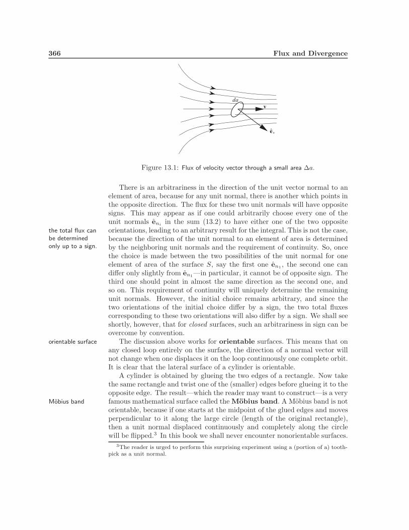
where x is the distance from the midpoint of the river and w is the width of theriver. Let us find the flux of the velocity, assuming that the cross section of the riveris a rectangle with depth equal to h, as shown in Figure 13.2.

The normal to the area da is perpendicular to the xy-plane and is in the samedirection as the velocity. Thus, we have v · da = v da = v dx dy, and

φ =

# #

S

v dx dy =

# h/2

−h/2

dy

# w/2

−w/2

v0

!1 − 4x2

w2

"dx

= hv0

# w/2

−w/2

!1 − 4x2

w2

"dx = hv0 (w − 1

3 w) = 23Av0,

where S is the cross section of the river and A is its area. !

The concept of flux, although indicative of a flow, is not limited to thevelocity vector field. We can define the flux of any vector field A in exactly

flux can be definednot only forvelocity, but forany vector field.the same way:

φ =# #

S

A · da. (13.3)

Whether such a definition is useful or not should be determined by experi-ment. It turns out that the flux of every physically relevant vector field isnot only useful, but essential for the theoretical—as well as experimental—investigation of that field. For example, the flux of a gravitational fieldthrough a closed surface is related to the amount of mass in the volumeenclosed in the surface. Similarly, the rate of change of the flux of a magneticfield through a surface gives the electric field produced at the boundary of thesurface.

ˆ e nO

x

y

da = dx dy

Figure 13.2: The river with its cross section.


θ

θ

Ee n

dϕϕ

a

x

y

dr

q

ρ

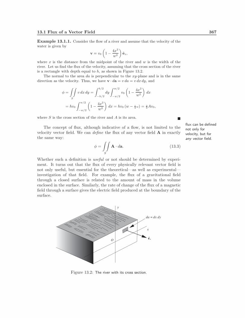
Figure 13.3: The flux of the electric field through a circle. The normal unit vector en

could be chosen to be either up or down. We choose (quite arbitrarily) the up directionto make the flux positive for positive q.

Example 13.1.2. Consider the flux of the electric field of a point charge locatedat a distance d from the center of a circle of radius a as shown in Figure 13.3. Theelement of flux is given by

E · da = |E| cos θda = |E| cos θρdρdϕ =kqr2

drρdρdϕ =

kqd

(d2 + ρ2)3/2ρdρdϕ,

where en is chosen to point up. The polar coordinates (ρ, ϕ) are used to specify apoint in the plane of the circle at which point the element of area is ρ dρ dϕ. To findthe total flux, we integrate the last expression above:

φ =

! !

S

kqd(d2 + ρ2)3/2

ρ dρ dϕ = kqd

! 2π

0

dϕ

! a

0

ρ dρ(d2 + ρ2)3/2

= 2πkqd"−(d2 + ρ2)−1/2

###a

0

$= 2πkq

%1 − d√

d2 + a2

&.

Note that since d represents a distance, as opposed to a coordinate, it is alwayspositive and d =

√d2 = |d|. !

It is often necessary to calculate the flux of a vector field through a closedsurface bounding a volume. Intuitively, such a flux gives a measure of thefor a closed

surface, one canuniquelydetermine thedirection ofnormal at eachpoint of thesurface.

strength of the source of the vector field in the volume. For instance, the fluxof the velocity field of water through a closed surface bounding a fountainmeasures the rate of the water output of the fountain. If the surface doesnot enclose the fountain, the net flux will be zero because the flux throughone “side” of the closed surface will be positive and that of the other “side”will be negative with the total flux vanishing. In the case of an electrostaticfield, the flux through a closed surface measures the amount of charge in thevolume bounded by that surface. The sign of the flux requires an orientationof the bounding surface which is equivalent to the assignment of a positivedirection to the unit normal to the surface at each of its points. We agree toout is positive!adhere to the convention of Box 12.1.3.4

4Only orientable surfaces can have a well defined orientation. Since we are excludingnonorientable surfaces from this book, all our surfaces respect Box 12.1.3.

13.1 Flux of a Vector Field 369

Example 13.1.3. Let us consider the flux through a sphere of radius a centeredat the origin of a vector field A given by A = kQrmer with k a proportionalityconstant and Q the strength of the source. Assuming that the outward normal isconsidered positive (see Box 12.1.3) the total flux through the sphere is calculatedas

φQ =

! !

S

A · da =

! !

S

kQamer · (era2 sin θ dθ dϕ)

= kQ

! 2π

0

dϕ

! π

0

ama2 sin θ dθ = 2πkQam+2! π

0

sin θ dθ = 4πkQam+2.

It is important to keep in mind that when calculating the flux of a vector field, one remember toevaluate thevector field at thesurface whencalculating itsflux!

has to evaluate the field at the surface. That is why a appears in the integral ratherthan r. Notice how the flux depends on the radius of the sphere. If m+ 2 > 0, thenthe farther away one moves from the origin, the more total flux passes through thesphere. On the other hand, if m + 2 < 0, although the size of the sphere increases,and therefore, more area is available for the field to cross, the field decreases toorapidly to give enough flux to the large sphere, so the flux decreases. The importantcase of m = −2 eliminates the dependence on a: The total flux through spheres ofdifferent sizes is constant. This last statement is a special case of the content of thecelebrated Gauss’s law. !

Historical NotesSpace vectors were conceived as three-dimensional generalizations of complex num-bers. The primary candidates for such a generalization however turned out to bequaternions—discovered by Hamilton—which had four components. One could nat-urally divide a quaternion into its “scalar” component and its vector component,the latter itself consisting of three components. The product of two quaternions,being itself a quaternion, can also be divided into scalar and vector parts. It turnsout that the scalar part of the product contains the dot product of the vector parts,and the vector part of the product contains the cross product of the vector parts.However, the full product contains some extra terms.

Physicists, on the other hand, were seeking a concept that was more closelyassociated with Cartesian coordinates than quaternions were. The first step in thisdirection was taken by James Clerk Maxwell. Maxwell singled out the scalar and thevector parts of Hamilton’s quaternion and put the emphasis on these separate parts.In his celebrated A Treatise on Electricity and Magnetism (1873) he does speak ofquaternions but treats the scalar and the vector parts separately.

Hamilton also developed a calculus of quaternions. In fact, the gradient operatorintroduced in Definition 12.3.2 and its name “nabla” were both Hamilton’s inven-tion.5 Hamilton showed that if ∇ acts on the vector part v of a quaternion, theresult will be a quaternion. Maxwell recognized the scalar part of this quaternionto be the divergence (to be discussed in the next section) of the vector v, and thevector part to be the curl (to be discussed in the Section 14.2) of v.

Maxwell often used quaternions as the basic mathematical entity or he at leastmade frequent reference to quaternions, perhaps to help his readers. Nevertheless,his work made it clear that vectors were the real tool for physical thinking and notjust an abbreviated scheme of writing, as some mathematicians maintained. Thus

5He used the word “nabla” because ∇ looks like an ancient Hebrew instrument of thatname.


by Maxwell’s time a great deal of vector analysis was created by treating the scalarand vector parts of quaternions separately.

The formal break with quaternions and the inauguration of a new independentsubject, vector analysis, was made independently by Josiah Willard Gibbs and OliverHeaviside in the early 1880s.

13.1.1 Flux Through an Arbitrary Surface

It may be useful to have a general formula for calculating the flux throughan arbitrary surface whose equation is given in parametric form in Cartesiancoordinates. Let

x = f(u, v), y = g(u, v), z = h(u, v), (13.4)

be the parametric equation of a surface. When v is held fixed and u is allowedto vary, a curve is traced on the surface whose infinitesimal displacement canbe written as [see Equation (6.63)]

dl1 = ex∂f

∂udu + ey

∂g

∂udu + ez

∂h

∂udu.

Similarly infinitesimal displacement along curves of constant u is

dl2 = ex∂f

∂vdv + ey

∂g

∂vdv + ez

∂h

∂vdv.

The cross product of these two displacements is the element of area of thesurface:

da = dl1 × dl2 = det

⎛

⎜⎜⎜⎜⎝

ex ey ez

∂f∂u

∂g∂u

∂h∂u

∂f∂v

∂g∂v

∂h∂v

⎞

⎟⎟⎟⎟⎠dudv ≡ det

⎛

⎜⎜⎜⎜⎝

ex ey ez

∂x∂u

∂y∂u

∂z∂u

∂x∂v

∂y∂v

∂z∂v

⎞

⎟⎟⎟⎟⎠dudv.

Using this in (13.3) we get

φ =∫ ∫

R

det

⎛

⎜⎜⎜⎜⎝

Ax Ay Az

∂x∂u

∂y∂u

∂z∂u

∂x∂v

∂y∂v

∂z∂v

⎞

⎟⎟⎟⎟⎠du dv, (13.5)

where Ax, Ay, and Az are considered functions of u and v obtained by substi-tuting (13.4) for their arguments. Equation (13.5) is an integral over a regionR in the uv-plane determined by the range of the variables u and v sufficientto describe the surface S.

The special, but important case, of a surface given by z = f(x, y) deservesspecial attention. In this case the parametrization is

x = u, , y = v, z = f(u, v)

13.2 Flux Density = Divergence 371

and (13.5) yields

φ =∫ ∫

R

det

⎛

⎜⎜⎜⎜⎝

Ax Ay Az

1 0 ∂z∂u

0 1 ∂z∂v ,

⎞

⎟⎟⎟⎟⎠du dv

or, writing (x, y) for (u, v)

φ =∫ ∫

R

(−Ax

∂z

∂x− Ay

∂z

∂y+ Az

)dx dy, (13.6)

where R is the projection of the surface S onto the xy-plane.

13.2 Flux Density = Divergence

The connection between flux and the strength of the source of a vector fieldwas mentioned above. We now analyze this connection further. The variationin the strength of the source of a vector field is measured by the density ofthe source. For example, the variation in the strength—concentration—ofthe source of electrostatic (gravitational) field is measured by charge (mass)density. We expect this variation to influence the intensity of flux at variouspoints in space.

13.2.1 Flux Density

Densities are physical quantities treated locally. A local consideration of flux,therefore, requires the introduction of the notion of flux density:

notion of fluxdensity anddivergence of avector fieldintroduced

Box 13.2.1. Take a small volume around a point P , evaluate the total fluxof a vector field through the bounding surface of the volume, and dividethe result by the volume to get the flux density or divergence of thevector field at P .

We denote the flux density by ρφ for the moment. Later we shall introduceanother notation which is more commonly used.

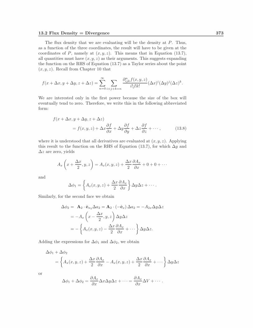
Let us quantify the discussion above for a vector field A. Consider a smallrectangular 6 volume ∆V centered at P with coordinates (x, y, z). Let thesides of the box be ∆x, ∆y, and ∆z as in Figure 13.4. We are interested in

6The rectangular shape of the volume is not a restriction because it will be made smallerand smaller at the end. In such a limit, any volume can be built from—a large number of—these small rectangular boxes. Compare this with the rectangular strips used in calculatingthe area under a curve.


e zAz

e yAy

e xAx

(x, y, z)

∆ x∆y

∆ z

A

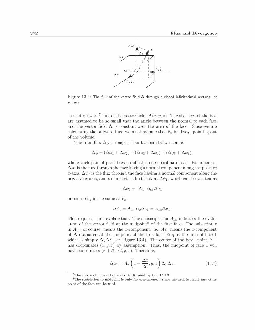
Figure 13.4: The flux of the vector field A through a closed infinitesimal rectangularsurface.

the net outward7 flux of the vector field, A(x, y, z). The six faces of the boxare assumed to be so small that the angle between the normal to each faceand the vector field A is constant over the area of the face. Since we arecalculating the outward flux, we must assume that en is always pointing outof the volume.

The total flux ∆φ through the surface can be written as

∆φ = (∆φ1 + ∆φ2) + (∆φ3 + ∆φ4) + (∆φ5 + ∆φ6),

where each pair of parentheses indicates one coordinate axis. For instance,∆φ1 is the flux through the face having a normal component along the positivex-axis, ∆φ2 is the flux through the face having a normal component along thenegative x-axis, and so on. Let us first look at ∆φ1, which can be written as

∆φ1 = A1 · en1∆a1

or, since en1 is the same as ex,

∆φ1 = A1 · ex∆a1 = A1x∆a1.

This requires some explanation. The subscript 1 in A1x indicates the evalu-ation of the vector field at the midpoint8 of the first face. The subscript xin A1x, of course, means the x-component. So, A1x means the x-componentof A evaluated at the midpoint of the first face; ∆a1 is the area of face 1which is simply ∆y∆z (see Figure 13.4). The center of the box—point P—has coordinates (x, y, z) by assumption. Thus, the midpoint of face 1 willhave coordinates (x + ∆x/2, y, z). Therefore,

∆φ1 = Ax

!x +

∆x

2, y, z

"∆y∆z. (13.7)

7The choice of outward direction is dictated by Box 12.1.3.8The restriction to midpoint is only for convenience. Since the area is small, any other

point of the face can be used.


The flux density that we are evaluating will be the density at P . Thus,as a function of the three coordinates, the result will have to be given at thecoordinates of P , namely at (x, y, z). This means that in Equation (13.7),all quantities must have (x, y, z) as their arguments. This suggests expandingthe function on the RHS of Equation (13.7) as a Taylor series about the point(x, y, z). Recall from Chapter 10 that

f(x + ∆x, y + ∆y, z + ∆z) =∞!

n=0

!

i+j+k=n

∂nijkf(x, y, z)

i!j!k!(∆x)i(∆y)j(∆z)k.

We are interested only in the first power because the size of the box willeventually tend to zero. Therefore, we write this in the following abbreviatedform:

f(x + ∆x, y + ∆y, z + ∆z)

= f(x, y, z) + ∆x∂f

∂x+ ∆y

∂f

∂y+ ∆z

∂f

∂z+ · · · , (13.8)

where it is understood that all derivatives are evaluated at (x, y, z). Applyingthis result to the function on the RHS of Equation (13.7), for which ∆y and∆z are zero, yields

Ax

"x +

∆x

2, y, z

#= Ax(x, y, z) +

∆x

2∂Ax

∂x+ 0 + 0 + · · ·

and

∆φ1 =$

Ax(x, y, z) +∆x

2∂Ax

∂x

%∆y∆z + · · · .

Similarly, for the second face we obtain

∆φ2 = A2 · en2∆a2 = A2 · (−ex)∆a2 = −A2x∆y∆z

= −Ax

"x − ∆x

2, y, z

#∆y∆z

= −$

Ax(x, y, z) − ∆x

2∂Ax

∂x+ · · ·

%∆y∆z.

Adding the expressions for ∆φ1 and ∆φ2, we obtain

∆φ1 + ∆φ2

=$

Ax(x, y, z) +∆x

2∂Ax

∂x− Ax(x, y, z) +

∆x

2∂Ax

∂x+ · · ·

%∆y∆z

or

∆φ1 + ∆φ2 =∂Ax

∂x∆x∆y∆z + · · · =

∂Ax

∂x∆V + · · · .


The reader may check that

∆φ3 + ∆φ4 =∂Ay

∂y∆V + · · · ,

∆φ5 + ∆φ6 =∂Az

∂z∆V + · · · , (13.9)

so that the total flux through the small box is

∆φ =!

∂Ax

∂x+

∂Ay

∂y+

∂Az

∂z

"∆V + · · · .

The flux density, or divergence as it is more often called, can now be obtainedby dividing both sides by ∆V and taking the limit as ∆V → 0. Since all theterms represented by dots are of at least the fourth order, they vanish in thelimit and we obtain

Theorem 13.2.1. The relation between the flux density of a vector field andthe derivatives of its components is

ρφ ≡ divA ≡ ∇ ·A = lim∆V →0

∆φ

∆V=

∂Ax

∂x+

∂Ay

∂y+

∂Az

∂z.

The term “divergence,” whose abbreviation is used as a symbol of fluxorigin of the term“divergence” density, is reminiscent of water flowing away from its source, a fountain. In

this context, the flux density measures how quickly or intensely water “di-verges” away from the fountain. The third notation ∇ · A combines thedot product in terms of components with the definition of ∇ as given inEquation (12.28).9

13.2.2 Divergence Theorem

The use of the word (volume) density for divergence suggests that the totalflux through a (large) surface should be the (volume) integral of divergence.However, any calculation of flux—even locally—requires a surface, as we sawin the derivation of flux density. What are the “small” surfaces used in thecalculation of flux density, and how is the large surface related to them? Theanswer to this question will come out of a treatment of an important theoremin vector calculus which we investigate now.

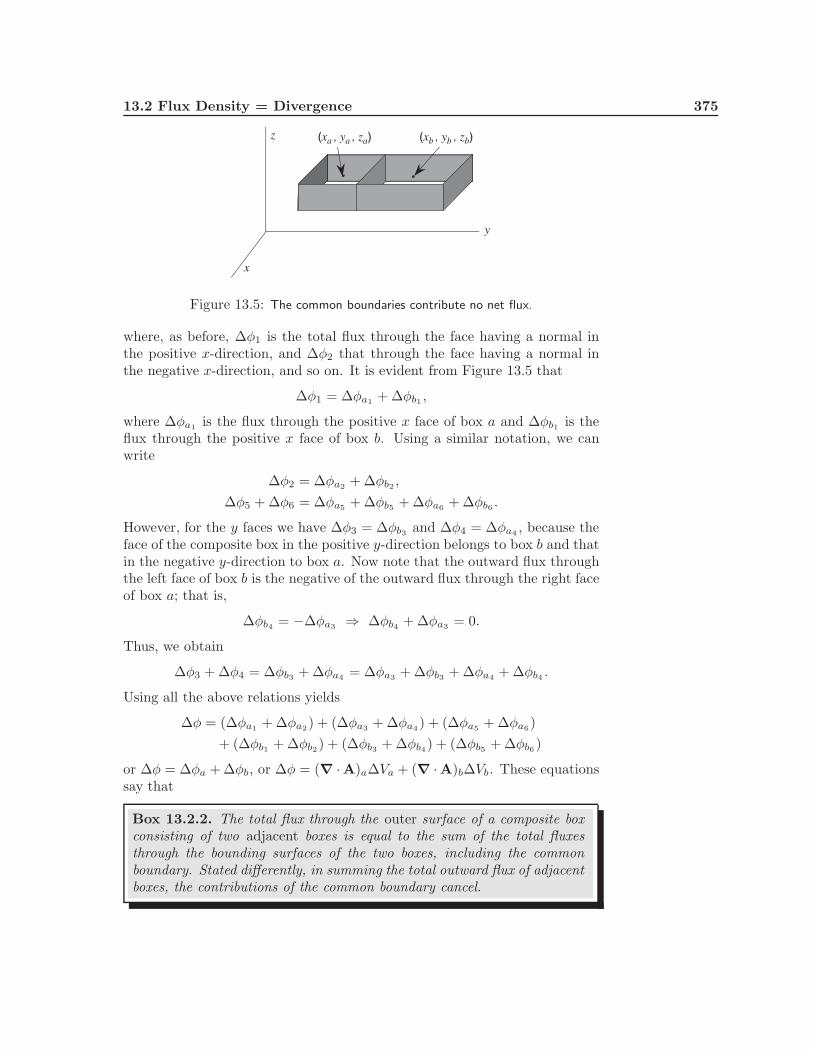
First consider two boxes with one face in common (Figure 13.5) and indexquantities related to the volume on the left by a and those related to the oneon the right by b. The total flux is, of course, the sum of the fluxes throughall six faces of the composite box :

∆φ = (∆φ1 + ∆φ2) + (∆φ3 + ∆φ4) + (∆φ5 + ∆φ6),9This notation is misleading because, as we shall see later, in non-Cartesian coordinate

systems, the expression of divergence in terms of derivatives will not be equal to simplythe dot product of ∇ with the vector field. One should really think of ∇ · A as a symbol,equivalent to ρφ or div A and not as an operation involving two vectors.


(xa , ya , za)

y

x

z (xb , yb , zb)

Figure 13.5: The common boundaries contribute no net flux.

where, as before, ∆φ1 is the total flux through the face having a normal inthe positive x-direction, and ∆φ2 that through the face having a normal inthe negative x-direction, and so on. It is evident from Figure 13.5 that

∆φ1 = ∆φa1 + ∆φb1 ,

where ∆φa1 is the flux through the positive x face of box a and ∆φb1 is theflux through the positive x face of box b. Using a similar notation, we canwrite

∆φ2 = ∆φa2 + ∆φb2 ,

∆φ5 + ∆φ6 = ∆φa5 + ∆φb5 + ∆φa6 + ∆φb6 .

However, for the y faces we have ∆φ3 = ∆φb3 and ∆φ4 = ∆φa4 , because theface of the composite box in the positive y-direction belongs to box b and thatin the negative y-direction to box a. Now note that the outward flux throughthe left face of box b is the negative of the outward flux through the right faceof box a; that is,

∆φb4 = −∆φa3 ⇒ ∆φb4 + ∆φa3 = 0.

Thus, we obtain

∆φ3 + ∆φ4 = ∆φb3 + ∆φa4 = ∆φa3 + ∆φb3 + ∆φa4 + ∆φb4 .

Using all the above relations yields

∆φ = (∆φa1 + ∆φa2) + (∆φa3 + ∆φa4) + (∆φa5 + ∆φa6)+ (∆φb1 + ∆φb2) + (∆φb3 + ∆φb4) + (∆φb5 + ∆φb6 )

or ∆φ = ∆φa + ∆φb, or ∆φ = (∇ ·A)a∆Va + (∇ ·A)b∆Vb. These equationssay that

Box 13.2.2. The total flux through the outer surface of a composite boxconsisting of two adjacent boxes is equal to the sum of the total fluxesthrough the bounding surfaces of the two boxes, including the commonboundary. Stated differently, in summing the total outward flux of adjacentboxes, the contributions of the common boundary cancel.


It is now clear how to generalize to a large surface bounding a volume: Di-vide up the volume into N rectangular boxes and write φ ≈

∑Ni=1(∇ ·A)i∆Vi.

The LHS of this equation is the outward flux through the bounding surfaceonly. Contributions from the sides of all inner boxes cancel out becauseeach face of a typical inner box is shared by another box whose outwardflux through that face is the negative of the outward flux of the original box.However, boxes at the boundary cannot find enough boxes to cancel all theirflux contributions, leaving precisely the flux through the original surface. Theuse of the approximation sign here reflects the fact that N , although large, isnot infinite, and that the boxes are not small enough. To attain equality wemust make the boxes smaller and smaller and their number larger and larger,in which case we approach the integral:

φ =∫ ∫

V

∫∇ ·A dV. (13.10)

Then, using Equation (13.2), we can state the importantthe veryimportantdivergencetheorem

Theorem 13.2.2. (Divergence Theorem). The surface integral (flux) ofany vector field A through a closed surface S bounding a volume V is equalto the volume integral of the divergence (or flux density) of A:

∫ ∫

S

A · da =∫ ∫

V

∫∇ ·A dV. (13.11)

Let A = cf where c is an arbitrary constant vector and f a function.Applying the divergence theorem to this A and using the readily verifiableidentity ∇ · (cf) = c · ∇f , we get

∫ ∫

S

fc·da =∫ ∫

V

∫c·(∇f)dV or c·

⎛

⎝∫ ∫

S

fda

⎞

⎠ = c·

⎛

⎝∫ ∫

V

∫(∇f)dV

⎞

⎠

Since this holds for any c, we must have

∫ ∫

S

fda =∫ ∫

V

∫∇fdV (13.12)

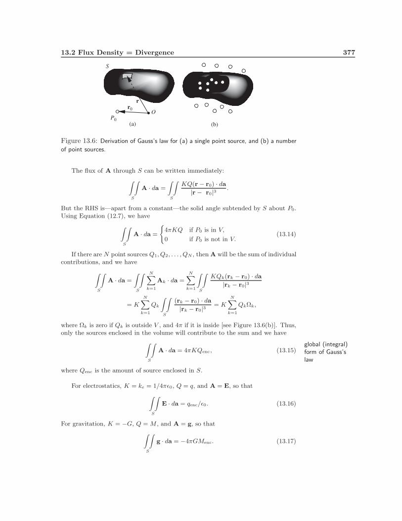
Example 13.2.3. In this example we derive Gauss’s law for fields which varyas the inverse of distance squared, specifically, gravitational and electrostatic fields.Let Q be a source point (a point charge or a point mass) located at P0 with positionvector r0 and S a closed surface bounding a volume V . Let A(r) denote the fieldproduced by Q at the field point P with position vector r as shown in Figure 13.6(a).We know that

A(r) =KQ

|r − r0|3(r− r0). (13.13)


S

OP0

rr0

(a) (b)

Figure 13.6: Derivation of Gauss’s law for (a) a single point source, and (b) a numberof point sources.

The flux of A through S can be written immediately:

! !

S

A · da =

! !

S

KQ(r − r0) · da|r − r0|3

.

But the RHS is—apart from a constant—the solid angle subtended by S about P0.Using Equation (12.7), we have

! !

S

A · da =

"4πKQ if P0 is in V,

0 if P0 is not in V.(13.14)

If there are N point sources Q1, Q2, . . . , QN , then A will be the sum of individualcontributions, and we have

! !

S

A · da =

! !

S

N#

k=1

Ak · da =N#

k=1

! !

S

KQk(rk − r0) · da|rk − r0|3

= KN#

k=1

Qk

! !

S

(rk − r0) · da|rk − r0|3

= KN#

k=1

QkΩk,

where Ωk is zero if Qk is outside V , and 4π if it is inside [see Figure 13.6(b)]. Thus,only the sources enclosed in the volume will contribute to the sum and we have

! !

S

A · da = 4πKQenc, (13.15)

where Qenc is the amount of source enclosed in S.

global (integral)form of Gauss’slaw

For electrostatics, K = ke = 1/4πϵ0, Q = q, and A = E, so that

! !

S

E · da = qenc/ϵ0. (13.16)

For gravitation, K = −G, Q = M , and A = g, so that

! !

S

g · da = −4πGMenc. (13.17)


The minus sign appears in the gravitational case because of the permanent attractionof gravity. Gauss’s law is very useful in calculating the fields of very symmetric sourcedistributions, and it is put to good use in introductory electromagnetic discussions.The derivation above shows that it is just as useful in gravitational calculations. !

Equation (13.15) is the integral or global form of Gauss’s law. We can alsoderive the differential or local form of Gauss’s law by invoking the divergencetheorem and assigning a volume density ρQ to Qenc:

LHS =! !

V

!∇ · A dV, RHS = 4πK

! !

V

!ρQ dV.

Since these relations are true for arbitrary V , we obtainlocal (differential)form of Gauss’slaw Theorem 13.2.4. (Differential Form of Gauss’s Law). If a point source

produces a vector field A that obeys Equation (13.13), then for any volumedistribution ρQ of the source we have ∇ · A = 4πKρQ.

This can easily be specialized to the two cases of interest, electrostaticsand gravity.

13.2.3 Continuity Equation

To improve our physical intuition of divergence, let us consider the flow of afluid of density ρ(x, y, z, t) and velocity v(x, y, z, t). The arguments to followare more general. They can be applied to the flow (bulk motion) of manyphysical quantities such as charge, mass, energy, momentum, etc. All thatneeds to be done is to replace ρ—which is the mass density for the fluidflow—with the density of the physical quantity.

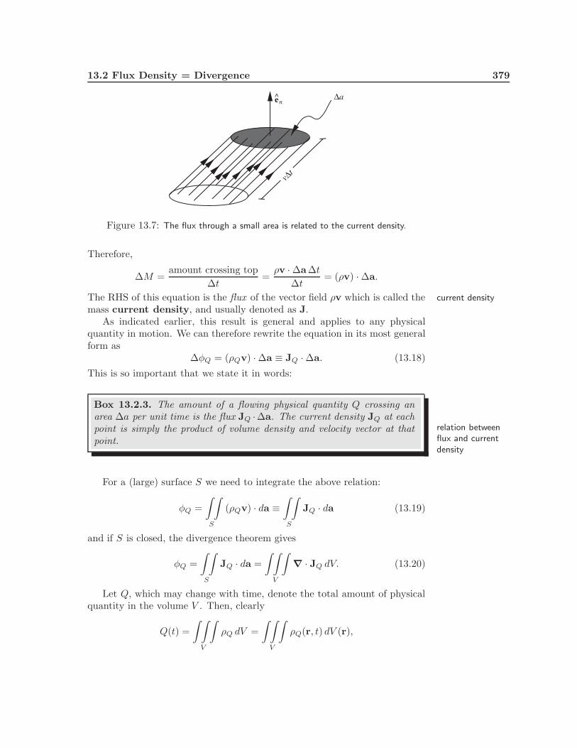
We are interested in the amount of matter crossing a surface area ∆aper unit time. We denote this quantity momentarily by ∆M , and becauseof its importance and wide use in various areas of physics, we shall deriveit in some detail. Take a small volume ∆V of the fluid in the shape of aslanted cylinder. The lateral side of this volume is chosen to be instantaneouslyin the same direction as the velocity v of the particles in the volume. Forlarge volumes this may not be possible, because the macroscopic motion ofparticles is, in general, not smooth, with different parts having completelydifferent velocities. However, if the volume ∆V (as well as the time intervalof observation) is taken small enough, the variation in the velocity of theenclosed particles will be negligible. This situation is shown in Figure 13.7.The lateral length of the cylinder is v∆t where ∆t is the time it takes theparticles inside to go from the base to the top, so that all particles inside willhave crossed the top of the cylinder in this time interval. Thus, we have

amount crossing top = amount in ∆V = ρ∆V.

But ∆V = (v∆t) · ∆a = v · ∆a∆t, where the dot product has been usedbecause the base and the top are not perpendicular to the lateral surface.


v∆t

ne ∆a

Figure 13.7: The flux through a small area is related to the current density.

Therefore,

∆M =amount crossing top

∆t=

ρv · ∆a∆t

∆t= (ρv) · ∆a.

The RHS of this equation is the flux of the vector field ρv which is called the current densitymass current density, and usually denoted as J.

As indicated earlier, this result is general and applies to any physicalquantity in motion. We can therefore rewrite the equation in its most generalform as

∆φQ = (ρQv) · ∆a ≡ JQ · ∆a. (13.18)This is so important that we state it in words:

Box 13.2.3. The amount of a flowing physical quantity Q crossing anarea ∆a per unit time is the flux JQ ·∆a. The current density JQ at eachpoint is simply the product of volume density and velocity vector at thatpoint.

relation betweenflux and currentdensity

For a (large) surface S we need to integrate the above relation:

φQ =! !

S

(ρQv) · da ≡! !

S

JQ · da (13.19)

and if S is closed, the divergence theorem gives

φQ =! !

S

JQ · da =! !

V

!∇ · JQ dV. (13.20)

Let Q, which may change with time, denote the total amount of physicalquantity in the volume V . Then, clearly

Q(t) =! !

V

!ρQ dV =

! !

V

!ρQ(r, t) dV (r),


where in the last integral we have emphasized the dependence of various quan-tities on location and time. Now, if Q is a conserved quantity such as energy,momentum, charge, or mass,10 the amount of Q that crosses S outward (i.e.,the flux through S) must precisely equal the rate of depletion of Q in thevolume V .global or integral

form of continuityequation

Theorem 13.2.5. In mathematical symbols, the conservation of a conservedphysical quantity Q is written as

dQ

dt= −

! !

S

JQ · da, (13.21)

which is the global or integral form of the continuity equation.

The minus sign ensures that positive flux gives rise to a depletion, andvice versa. The local or differential form of the continuity equation can beobtained as follows: The LHS of Equation (13.21) can be written as

dQ

dt=

d

dt

! !

V

!ρQ(r, t) dV (r) =

! !

V

!∂ρQ

∂t(r, t) dV (r),

while the RHS, with the help of the divergence theorem, becomes

−! !

S

JQ · da = −! !

V

!∇ · JQ dV.

Together they give! !

V

!∂ρQ

∂tdV = −

! !

V

!∇ · JQ dV

or! !

V

! "∂ρQ

∂t+ ∇ · JQ

#dV = 0.

This relation is true for all volumes V . In particular, we can make the volumeas small as we please. Then, the integral will be approximately the integrandtimes the volume. Since the volume is nonzero (but small), the only way thatthe product can be zero is for the integrand to vanish.

Box 13.2.4. The differential form of the continuity equation is

∂ρQ

∂t+ ∇ · JQ = 0. (13.22)

local (differential)form of continuityequation

10In the theory of relativity mass by itself is not a conserved quantity, but mass incombination with energy is.


Both integral and differential forms of the continuity equation have a widerange of applications in many areas of physics.

Equation (13.22) is sometimes written in terms of ρQ and the velocity.This is achieved by substituting ρQv for JQ:

∂ρQ

∂t+ ∇ · (ρQv) = 0

or∂ρQ

∂t+ (∇ρQ) · v + ρQ∇ · v = 0.

However, using Cartesian coordinates, we write the sum of the first two termsas a total derivative:

∂ρQ

∂t+ (∇ρQ) · v =

∂ρQ

∂t+

!∂ρQ

∂x,∂ρQ

∂y,∂ρQ

∂z

"·!

dx

dt,dy

dt,dz

dt

"

=∂ρQ

∂t+

∂ρQ

∂x

dx

dt+

∂ρQ

∂y

dy

dt+

∂ρQ

∂z

dz

dt# $% &=total derivative=dρQ/dt

=dρQ

dt.

Thus the continuity equation can also be written as

dρQ

dt+ ρQ∇ · v = 0. (13.23)

Historical NotesAside from Maxwell, two names are associated with vector analysis (completelydetached from their quaternionic ancestors): Willard Gibbs and Oliver Heaviside.

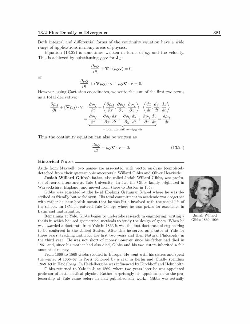
Josiah Willard Gibbs’s father, also called Josiah Willard Gibbs, was profes-sor of sacred literature at Yale University. In fact the Gibbs family originated inWarwickshire, England, and moved from there to Boston in 1658.

Gibbs was educated at the local Hopkins Grammar School where he was de-scribed as friendly but withdrawn. His total commitment to academic work togetherwith rather delicate health meant that he was little involved with the social life ofthe school. In 1854 he entered Yale College where he won prizes for excellence inLatin and mathematics.

Josiah WillardGibbs 1839–1903

Remaining at Yale, Gibbs began to undertake research in engineering, writing athesis in which he used geometrical methods to study the design of gears. When hewas awarded a doctorate from Yale in 1863 it was the first doctorate of engineeringto be conferred in the United States. After this he served as a tutor at Yale forthree years, teaching Latin for the first two years and then Natural Philosophy inthe third year. He was not short of money however since his father had died in1861 and, since his mother had also died, Gibbs and his two sisters inherited a fairamount of money.

From 1866 to 1869 Gibbs studied in Europe. He went with his sisters and spentthe winter of 1866–67 in Paris, followed by a year in Berlin and, finally spending1868–69 in Heidelberg. In Heidelberg he was influenced by Kirchhoff and Helmholtz.

Gibbs returned to Yale in June 1869, where two years later he was appointedprofessor of mathematical physics. Rather surprisingly his appointment to the pro-fessorship at Yale came before he had published any work. Gibbs was actually


a physical chemist and his major publications were in chemical equilibrium andthermodynamics. From 1873 to 1878, he wrote several important papers on ther-modynamics including the notion of what is now called the Gibbs potential.

Gibbs’s work on vector analysis was in the form of printed notes for the use ofhis own students written in 1881 and 1884. It was not until 1901 that a properlypublished version appeared, prepared for publication by one of his students. Usingideas of Grassmann, a high school teacher who also worked on the generalization ofcomplex numbers to three dimensions and invented what is now called Grassmannalgebra, Gibbs produced a system much more easily applied to physics than that ofHamilton.

His work on statistical mechanics was also important, providing a mathematicalframework for the earlier work of Maxwell on the same subject. In fact his lastpublication was Elementary Principles in Statistical Mechanics, which is a beautifulaccount putting statistical mechanics on a firm mathematical foundation.

Except for his early years and the three years in Europe, Gibbs spent his wholelife living in the same house which his father had built only a short distance from theschool Gibbs had attended, the college at which he had studied, and the universitywhere he worked all his life.

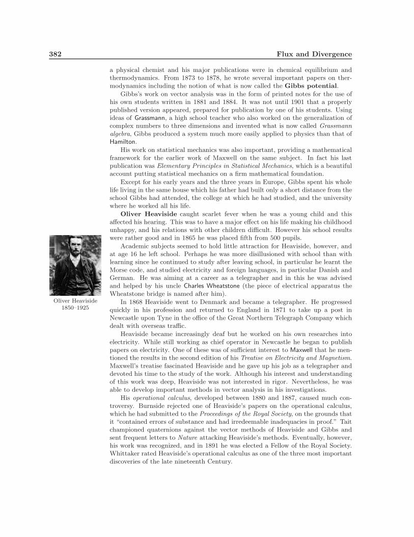
Oliver Heaviside caught scarlet fever when he was a young child and thisaffected his hearing. This was to have a major effect on his life making his childhoodunhappy, and his relations with other children difficult. However his school resultswere rather good and in 1865 he was placed fifth from 500 pupils.

Academic subjects seemed to hold little attraction for Heaviside, however, andat age 16 he left school. Perhaps he was more disillusioned with school than withlearning since he continued to study after leaving school, in particular he learnt theMorse code, and studied electricity and foreign languages, in particular Danish andGerman. He was aiming at a career as a telegrapher and in this he was advisedand helped by his uncle Charles Wheatstone (the piece of electrical apparatus theWheatstone bridge is named after him).

Oliver Heaviside1850–1925

In 1868 Heaviside went to Denmark and became a telegrapher. He progressedquickly in his profession and returned to England in 1871 to take up a post inNewcastle upon Tyne in the office of the Great Northern Telegraph Company whichdealt with overseas traffic.

Heaviside became increasingly deaf but he worked on his own researches intoelectricity. While still working as chief operator in Newcastle he began to publishpapers on electricity. One of these was of sufficient interest to Maxwell that he men-tioned the results in the second edition of his Treatise on Electricity and Magnetism.Maxwell’s treatise fascinated Heaviside and he gave up his job as a telegrapher anddevoted his time to the study of the work. Although his interest and understandingof this work was deep, Heaviside was not interested in rigor. Nevertheless, he wasable to develop important methods in vector analysis in his investigations.

His operational calculus, developed between 1880 and 1887, caused much con-troversy. Burnside rejected one of Heaviside’s papers on the operational calculus,which he had submitted to the Proceedings of the Royal Society, on the grounds thatit “contained errors of substance and had irredeemable inadequacies in proof.” Taitchampioned quaternions against the vector methods of Heaviside and Gibbs andsent frequent letters to Nature attacking Heaviside’s methods. Eventually, however,his work was recognized, and in 1891 he was elected a Fellow of the Royal Society.Whittaker rated Heaviside’s operational calculus as one of the three most importantdiscoveries of the late nineteenth Century.

13.3 Problems 383

Heaviside seemed to become more and more bitter as the years went by. In 1908he moved to Torquay where he showed increasing evidence of a persecution complex.His neighbors related stories of Heaviside as a strange and embittered hermit whoreplaced his furniture with granite blocks which stood about in the bare rooms likethe furnishings of some Neolithic giant. Through those fantastic rooms he wandered,growing dirtier and dirtier, with one exception: His nails were always exquisitelymanicured, and painted a glistening cherry pink.

13.3 Problems

13.1. Using (13.6) find the flux of the vector field A = kx2ez through theportion of the sphere of radius a centered at the origin lying in the first octantof a Cartesian coordinate system.

13.2. Using (13.6) find the flux of the vector field A = yex + 3zey − 2xez

through the portion of the plane x + 2y − 3z = 5 lying in the first octant of aCartesian coordinate system.

13.3. A vector field is given by A = r. Using (13.6) find the flux of thisvector field through the upper hemisphere centered at the origin. Verify youranswer by calculating the flux using (the much easier) spherical coordinates.

13.4. Find the flux of the vector field A = x2ex + y2ey + z2ez through theportion of the plane x + y + z = 1 lying in the first octant of a Cartesiancoordinate system.

13.5. Using (13.6), find the flux of the vector field A = kr/r3 through theupper hemisphere centered at the origin. Verify your answer by calculatingthe flux using spherical coordinates.

13.6. Find the flux of the vector field A = yey + aez through the portion ofthe paraboloid z = b2 − x2 − y2 above the xy-plane.

13.7. Derive Equation (13.9).

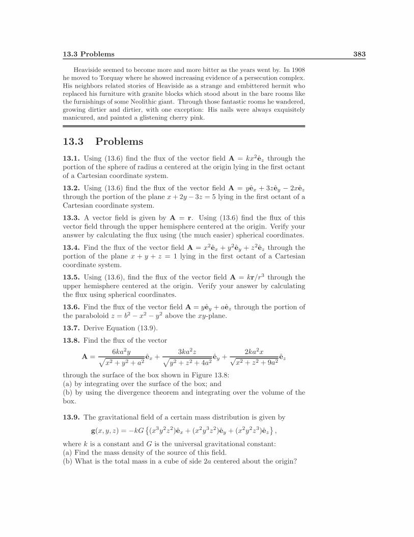
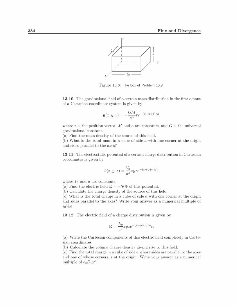
13.8. Find the flux of the vector

A =6ka2y!

x2 + y2 + a2ex +

3ka2z!y2 + z2 + 4a2

ey +2ka2x√

x2 + z2 + 9a2ez

through the surface of the box shown in Figure 13.8:(a) by integrating over the surface of the box; and(b) by using the divergence theorem and integrating over the volume of thebox.

13.9. The gravitational field of a certain mass distribution is given by

g(x, y, z) = −kG"(x3y2z2)ex + (x2y3z2)ey + (x2y2z3)ez

#,

where k is a constant and G is the universal gravitational constant:(a) Find the mass density of the source of this field.(b) What is the total mass in a cube of side 2a centered about the origin?


x

y

z

2a

3a

a

Figure 13.8: The box of Problem 13.8.

13.10. The gravitational field of a certain mass distribution in the first octantof a Cartesian coordinate system is given by

g(x, y, z) = −GM

a3re−(x+y+z)/a,

where r is the position vector, M and a are constants, and G is the universalgravitational constant.(a) Find the mass density of the source of this field.(b) What is the total mass in a cube of side a with one corner at the originand sides parallel to the axes?

13.11. The electrostatic potential of a certain charge distribution in Cartesiancoordinates is given by

Φ(x, y, z) =V0

a3xyze−(x+y+z)/a,

where V0 and a are constants.(a) Find the electric field E = −∇Φ of this potential.(b) Calculate the charge density of the source of this field.(c) What is the total charge in a cube of side a with one corner at the originand sides parallel to the axes? Write your answer as a numerical multiple ofϵ0V0a.

13.12. The electric field of a charge distribution is given by

E =E0

a4xyze−(x+y+z)/ar.

(a) Write the Cartesian components of this electric field completely in Carte-sian coordinates.(b) Calculate the volume charge density giving rise to this field.(c) Find the total charge in a cube of side a whose sides are parallel to the axesand one of whose corners is at the origin. Write your answer as a numericalmultiple of ϵ0E0a2.

13.3 Problems 385

13.13. The velocity of a physical quantity Q is radial and given by v = krwhere k is a constant. Show that if the density ρQ is independent of position,then it is given by

ρQ(t) = ρ0Qe−3kt

where ρ0Q is the initial density of Q.

flux and divergence

Documents