KULLBACK–LEIBLER DIVERGENCE FOR EVALUATINGBIOEQUIVALENCE:

II. Simulation and Retrospective Assessment of Performance of the ProposedFDA metric and the Kullback-Leibler Divergence in Individual Bioequivalence

Assessment

Scott D Patterson, Vladimir Dragalin, Valerii Fedorov, and Byron Jones

GSK BDS Technical Report 2001 – 02

17 August 2001

This paper was reviewed and recommended for publication by

Stephen Senn, University College, London

and

Henry Wynn, University of Warwick, Coventry

Copyright c© 2001 by GlaxoSmithKline Pharmaceuticals

Biostatistics and Data Sciences

GlaxoSmithKline Pharmaceuticals

1250 South Collegeville Road, POBox 5089

Collegeville, PA, 19426–0989, USA

KULLBACK–LEIBLER DIVERGENCE FOR EVALUATING

BIOEQUIVALENCE:

II. Simulation and Retrospective Assessment of Performance of the Proposed FDA metric and

the Kullback-Leibler Divergence in Individual Bioequivalence Assessment

Scott D Patterson, Vladimir Dragalin, Valerii Fedorov, and Byron Jones

Biostatistics and Data Sciences, GlaxoSmithKline Pharmaceuticals

Abstract. Methodology has been proposed for evaluating switchability of two formulations of a drug

that encompasses bioequivalence aspects using Dragalin and Fedorov’s application of the Kullback-

Leibler Divergence (KLD) and a metric developed by the Food and Drug Administration (FDA) as

measures of discrepancy between the distributions of the two formulations using two sequence replicate,

crossover designs.

Standards are proposed for implementation of the KLD as an alternative procedure for the evaluation

of similarity between formulations using the same study design as that proposed in FDA guidance.

Simulations are conducted to evaluate the performance of the KLD relative to the metric proposed in

guidance by the Food and Drug Administration for the evaluation of individual bioequivalence.

Previously published retrospective analyses using the FDA proposed metric are contrasted with

those based on the KLD, and thoughts regarding future evaluations are explored. This investigation is

conducted to provide an exploratory look into the properties of the two metrics in order to support a

future, rigorous comparison.

It is concluded that the KLD is a viable alternative to the FDA-proposed metric and that its math-

ematical properties make it a readily interpretable measure of the individual differences between formu-

lations.

1. Introduction

Bioequivalence trials play a key role in the drug development process and are used by pharmaceutical

sponsors who have conducted pivotal efficacy trials with a specific formulation of a drug therapy but want

market access for a more commercially suitable formulation or when a substantial formulation change is

sought post-approval. These studies are also used by the generic pharmaceutical industry to gain market

access for new formulations of established drug therapies when the patent of the sponsor’s formulation

expires. Rather than repeat clinical trials to establish the safety and efficacy of the proposed formulations,3

4

the pharmacokinetic (PK) characteristics of the plasma-concentration time curve are used to infer that

two drug formulations will provide similar therapeutic benefit.

PK is expressed in terms of rate and extent of absorption as characterized by the maximum observed

plasma concentration (Cmax) and the area under the concentration time curve (AUC). Bioequivalence

is expressed in terms of the ’similarity’ of these two metrics between the two formulations.

Average bioequivalence (ABE; FDA Guidance, 1992-2000) has traditionally been used as the standard for

market access with regulatory limits of twenty percent. This approach focuses on the average PK metrics

of the two formulations being studied. The framework for statistical inference is based on ninety percent

confidence intervals for the mean differences and is currently being used for both instances of pre-market

approval and post-market formulation changes described above. The two one-sided hypotheses of interest

(Schuirmann, 1987) are:

H01 : µT − µR≤− loge1.25 (1)

or

H02 : µT − µR≥loge1.25 (2)

versus

HA : −loge1.25 < µT − µR < loge1.25 (3)

where µT and µR represent mean of the Test and Reference formulations, respectively, and the limit of

loge1.25 is chosen to represent a twenty percent range on the loge-scale. PK data such as AUC and Cmax

are typically held to be log-normally distributed (Westlake, 1986) and are treated as normally distributed

following appropriate transformation (usually log to base e transformation). Inference is based on the

use of the non-central t-distribution using a model appropriate to a randomised, two-period crossover

design. AUC and Cmax are analyzed separately, and each one-sided test is performed at the five percent

level. No adjustments for multiplicity are made (Hauck et al., 1995).

In practical terms, a ninety percent confidence interval is constructed on the estimated difference µT−µR.

If the confidence interval falls within the range −loge1.25 to loge1.25, then average bioequivalence is

5

demonstrated. More commonly, this difference and confidence interval is exponentiated and assessed

relative to the interval 0.80 to 1.25.

Following the original proposal in 1997 (cf. FDA Guidance), in August 1999, the FDA re-proposed

new guidelines for the assessment of bioequivalence: population bioequivalence (PBE) and individual

bioequivalence (IBE) (FDA Guidances, 1999) based on ideas developed by Anderson (1993) and Anderson

and Hauck (1983, 1990). In the case of pre-market approval, one can formulate the bioequivalence

question as ”Can a patient begin therapy with either formulation (commercial or clinical trial) and be

assured similar results in terms of safety and efficacy?” This has been called the concept of prescribability

(Anderson and Hauck, 1990) and is linked to PBE. Aspects of PBE will be discussed in more detail in a

separate communication in preparation.

In the case of post marketing changes, the bioequivalence question becomes: ”Can I safely and effectively

switch my patient from their current formulation to another?” This has been called the concept of

switchability (Anderson and Hauck, 1990) and is linked to IBE. The criteria used to assess IBE under

the proposed FDA draft guidance (1997-1999) and FDA guidance (2000-2001) aggregates the difference

between population means and variances and accounts for subject predictability from one formulation to

the other (subject-by-formulation interaction, Ekbohm and Melander, 1989). In addition, the individual

bioequivalence metric allows for scaling of the regulatory limits based on the within-subject variability

of the reference product.

Extensive, international debate on the merits of the proposed FDA metrics occurred in the interval since

the original preliminary, draft guidance on population and individual bioequivalence was issued in 1997.

For a summary, see Patterson (2001a-b).

In bioequivalence studies, using replicated crossover designs, the following model for observations is

commonly accepted (Jones and Kenward, 1989). Let Xtjk be the k-th response (k = 1, 2, . . . ) for the

j-th subject in the cross-over trial administered formulation t (t = T,R) and

Xtjk = ξtj + εtjk = µt + νtj + εtjk (4)

νtj , the subject-by-formulation random effect,

εtjk, within-subject random effects for each formulation, are independent with mean zero,

V ar(νtj) = σ2Bt, the between-subject variance,

V ar(νTj − νRj) = σ2D = σ2

BT + σ2BR − 2ρσBT σBR, the subject-by-formulation interaction variance and,

Cov(νTj , νRj) = ρσBT σBR,

6

V ar(εtjk) = σ2Wt, the within-subject variance,

Cov(εtjk, εtjk′) = 0, for k 6= k′.

In practice, sequence and period effects would be taken into account in the model (Jones and Kenward,

1989; Senn, 1993) but are omitted here for simplicity. Carryover effects (Jones and Kenward, 1989) may

be fitted in certain situations and are also omitted. Two formulations are declared bioequivalent if the

upper bound of (1−α)100% confidence interval for the FDA metric is less than a predetermined goalpost

set by a regulator.

The following ’mixed-scaled’ criteria is recommended for IBE assessment (FDA Guidance, 1999):

(µT − µR)2 + σ2D + σ2

WT − σ2WR

max(0.04, σ2WR)

≤ ϑI (5)

where ϑI is a goalpost (see section 2.1). Because the within-subject variance of each treatment can not

usually be reliably and separately estimated in a two-way cross-over { TR, RT } (unless the assumption

that between-subject variability is homogeneous is made along with the assumption that correlation

is unity), a replicated design (a crossover with sequences { TRTR, RTRT } or { TRRT, RTTR } for

example) is required. Any multi-sequence, replicate design, crossover study in accordance with Vonesh

and Chinchilli (1997) may be used to estimate the moments of interest.

Note that, due to the nature of this ’aggregate’ FDA criteria, differences in means in this criteria can

be ’negated’ by decreased within-subject variance for the test formulation. Some have noted this to be

an undesirable property of the proposed metric, (Endrenyi and Hao, 1998), and it is known that such

trade-offs do occur in practice (Zariffa et al., 2000). Additionally, it should be noted that the between-

subject inconsistency of the test-reference comparison quantified by estimated σ2D might be an inadequate

measure of the switchability (Zariffa et al., 2000; Zariffa and Patterson, 2001).

While there is little to no evidence to suggest that the ABE criteria has failed to protect the public

(Barrett et al., 2000) and there has been considerable debate on the merits of the proposal (Senn,

2000), consumers may find these specific questions above related to PBE and IBE more relevant. One

reviewer noted recently that very little data have been published to assess how the proposed FDA criteria

performs (Colburn and Keefe, 2000). One of the key provisions of the 1999 draft FDA guidance is the

suggestion for what has been termed a ’public health experiment’ or mandatory data collection period

(Montreal, AAPS/FDA Workshop, August/September 1999). Sponsors of any bioequivalence study

would be compelled to submit data from a replicate design to FDA for approval to market. Subsequent

discussion at the Advisory Committee for Pharmaceutical Science (September 1999, Washington DC)

7

resulted in the recommendation that market access not be permitted unless average bioequivalence had

been demonstrated under existing criteria. Restricting the ’experiment’ to a class of drugs such as

controlled release formulation and highly variable drugs was also suggested.

The finalised FDA guidance (2000-2001) calls for the use of replicate designs for highly variable drug

products (σWR ≥ 0.30) and for modified-release products. Market access is restricted to those compounds

demonstrating average bioequivalence though sponsors may use PBE or IBE criteria if justified in the

protocol and with FDA’s prior consent. Thus, data in replicate designs will be accumulated in such drug

products over the next few years and may eventually be examined with the intent of determining whether

use of PBE and IBE criteria are warranted to protect public health.

This calls for careful and meticulous examination of existing replicate design data sets prior to beginning

the ’public health experiment’ so as to set realistic expectations for the exercise (Zariffa et al., 2000;

Zariffa and Patterson, 2001) and for the careful, scientific consideration of viable alternatives to the

procedure developed by the FDA. This report follows on from a previous report by Dragalin and Fedorov

(1999) introducing methodology relating to an alternative measure for bioequivalence assessment using the

properties of information and sufficiency of Kullback and Leibler (Kullback, 1968). The ideas presented

in Dragalin and Fedorov’s (1999) work are summarized from their paper below on the topic of IBE

assessment under a two-sequence, replicate design. It should be noted that other alternative, sequential

procedures have also recently been proposed (Barrett et al., 2000) but will not be addressed in this paper.

Under Dragalin and Fedorov’s application of the Kullback-Leibler Divergence, two formulations are de-

clared bioequivalent if the upper bound of (1 − α)100% confidence interval for the Kullback-Leibler

Divergence is less than a given goalpost to be set by a regulator. Consider a general model for obser-

vations (XRj , XTj) on subject j in a cross-over design that compares a test drug formulation T with

a reference drug formulation R. Assume that each observation Xtj has two components: the subject-

formulation effect ξtj and within-subject random error εtj . Let ϕ be the joint density of (ξR, ξT ), the

subject-formulation effects on the same subject. Let also fξ(x) be the density function for XRj and

similarly gξ(x) be the density function for XTj , conditional on the subject-formulation effects ξRj and

ξTj respectively. Then the KLD for IBE can be defined as

d(fT , fR) = Eϕ

[Ef log

fξ

gξ+ Eg log

gξ

fξ

]. (6)

where El denotes the expectation over some distribution l.

8

Suppose that for each subject in the trial at least a pair of (XRj , XTj) of observations is available.

Assuming that

XRj

∣∣∣νRj ∼ N (µR + νRj , σ2WR) and XTj

∣∣∣νTj ∼ N (µT + νTj , σ2WT )

where N (µ, σ2) is the normal distribution with mean µ and variance σ2, we can calculate as in (6)

the conditional KLD between the distributions of XRj and XTj , conditioned on j-th subject related

characteristics (νRj , νTj):

dν(fT , fR) =12

{(µT + νTj − µR − νRj)2 + σ2

WT + σ2WR

}( 1σ2

WT

+1

σ2WR

)− 2

Assuming additionally that (νRj , νTj) has a bivariate normal distribution with zero means, we can cal-

culate the unconditional KLD integrating out the effect of (νRj , νTj):

d(fT , fR) =12

{(µT − µR)2 + σ2

D + σ2WT + σ2

WR

}( 1σ2

WT

+1

σ2WR

)− 2 (7)

Dragalin and Fedorov called (7) the KLD for IBE. Notice that this measure of discrepancy is based on

the same parameters as the currently proposed FDA measure (5). However, the KLD for IBE fulfills the

desired properties of a discrepancy measure while the FDA proposed metric fails on all three properties of

a true discrepancy metric. Note that in general, the moments of interest are estimable only in a replicate

design study (Vonesh and Chinchilli, 1997) and when σ2WT = σ2

WR > 0.04, the FDA metric and the KLD

are equivalent.

A true discrepancy metric is defined as follows (cf. Dragalin and Fedorov, 1999). If F and G are

two distributions for formulations Test and Reference, respectively, on a general measurable space with

densities f and g respectively, then the discrepancy between f and g is denoted by ∆(f, g) with various

subscripts for particular cases. It may be verified that the KLD for IBE fulfills a few desired properties

of a true discrepancy metric (see more details in Dragalin and Fedorov, 1999):

1. ∆(f, g) ≥ 0 and∆(f, g) = 0 iff f = g;

2. ∆(f, g) = ∆(g, f);

3. ∆(f, g) is invariant with respect to any transform which preserves the existence of the KLD (for

instance any continuous transform);

4. Measures of IBE, PBE, and ABE based on the KLD follow a natural heirarchy such that demonstration

of IBE implies PBE which in turn implies ABE.

9

It should be noted that the FDA criteria for average, population, and individual bioequivalence (FDA

Guidances 1992, 1997, 1999a-b, 2000, 2001) do not meet any of the above definitions as known based on

findings described elsewhere (Zariffa et al., 2000; Zariffa and Patterson, 2001).

Statistical assessment of bioequivalence using the bioequivalence criteria discussed in this paper consists

of constructing one-sided confidence intervals for the KLD (7) and the FDA metric (5). Only Restricted

maximum likelihood (REML) and Bootstrap (FDA Guidance, 1997) or Method of Moment (MoM) based

approximate procedures (FDA Guidance, 1999a-b, 2001; Hyslop et al., 2000) currently have been proposed

for evaluation of the FDA metric. As method of moment based, approximate procedures have yet to

be validated and are known to produce negative variance components for the subject-by-formulation

interaction variance (Zariffa and Patterson, 2001), REML estimation (Patterson and Thompson, 1971) is

used to derive parameter estimates in this paper. This is in accordance with other recent investigations

on the topic (Hauck et al., 2000) although some concerns with positive bias in the estimates of variance

have been expressed in the statistical literature (Endrenyi and Tothfalusi, 1999). REML versus MoM

estimation of the components in the above mixed modelling equations will be the subject of a future

communication.

As an approximate method for deriving a confidence interval for the KLD is not yet available, the

bootstrap (Efron and Tibshirani, 1993) is used to assess inference in this preliminary investigation of the

KLD’s properties. The FDA metric is similarly assessed based on a bootstrap procedure in order to be

consistent, and it is noted that previous work (Patterson and Zariffa, 2000) has established that only a

small number of changes in inference are observed in an extensive database when using the approximate

procedure for inference on the FDA metric relative to the bootstrap. The bootstrap procedure is known

to yield consistent results for the FDA metric when within-subject variance estimates for the reference

product are not near the cutoff 0.04 (Shao et al., 2000a-b).

Section 2 describes simulations performed to evaluate the performance of the KLD relative to the FDA

proposed metric based upon a replicate design studies with sequences TRTR and RTRT given known

parameter quantities for the moments included in each metric. Goalposts are proposed for evaluation of

the KLD in actual studies. Section 3 describes retrospective analyses of twenty-two previously published

replicate design data sets (Zariffa et al., 2000), and contrasts results between the KLD and FDA metric.

Section 4 discusses the discrepancies between measures and describes research to be performed during

the upcoming data collection period to evaluate alternative approaches to the assessment of individual

bioequivalence. Future topics of research are described in Section 5.

10

2. Simulations

2.1. FDA compatible Goalposts in IBE Assessment. The goalpost for individual bioequivalence

assessment assumes a within-subject variance for the reference formulation of 0.04 and is set to 2.49

allowing for a mean difference of twenty percent and a variance allowance of 0.05 in the numerator under

the procedure proposed by the FDA (cf. FDA Guidance, 1999) and (5). If the upper 95% bound on

the FDA metric falls below this value of 2.49, individual bioequivalence is demonstrated for the endpoint

under study. Scaled to within-subject reference variation (again, assumed to be 0.04, under the FDA

Guidance 1997), the goalpost accounting for the means amounts to a value of 1.2443=(loge(1.25))2/0.04.

The remaining allowance, known as the ’variance allowance’ and is equal to 1.25, is composed of a value of

0.75 (accounting for allowable subject-by-formulation interaction of (σ2D/σ2

WR)=(0.03/0.04), when scaled

to within-subject reference product variation) and 0.5 (allowing for a difference in within-subject variances

((σ2WT − σ2

WR)/σ2WR)=(0.02/0.04), when scaled to reference product variation.)

Allowing for a mean difference of 20% and scaling all terms in (7) to within-subject reference product

variation (assumed to be 0.04), the corresponding goalpost for IBE assessment, using the values posited

by FDA above, for the KLD assessed using the replicate design can be shown to be 1.75. If the 95%

upper bound for the KLD falls below this value, individual bioequivalence assessment is demonstrated.

2.2. Methods. Our approach is based on the model from Section 1. True values for the moments of

interest are given, and data sets from a replicate design with sequences TRTR and RTRT are simulated

based on these values. Modelling procedures are then conducted on each data set to give point estimates

for the metrics of interest. The bootstrap procedure is then applied 2000 times to each simulated data

set, and each bootstrap sample is modelled. The upper 95th quantile of the estimates from the bootstrap

are upper ninety-five percent bounds for the metrics of interest.

Simulation method.

True values for the means and variances for the model described in Section 1 are given, and SAS IML

running under a UNIX machine was used to simulate data sets containing n=36 subjects in a replicate

design of the form TRTR and RTRT (n=18 subjects per sequence) on the loge-scale. One hundred data

sets were generated for each scenario as summarized in Table 1. Between-subject standard deviations

were twice the magnitude of within-subject standard deviations. Non-negligible values of σ2D were chosen

11

to be consistent with those levels discussed at the September 1999 Advisory Committee by FDA and are

derived as 0.75 times the within-subject variance for the reference formulation.

Simulations 1 and 2 were performed to calibrate the exercise (i.e. to confirm that, when the FDA metric

and KL Divergence should be zero, that they are estimated to be so) for a low and high variability drug

product, respectively.

Simulations 3 and 4 evaluate the FDA metric and KLD when a 20% difference in mean response is known

to exist between formulations for a low and high variability drug product, respectively. Simulations 5

and 6 evaluate the impact on the metrics when a 50% difference in within-subject variances is present in

addition to a 20% difference in means for a low and high variability drug product, respectively. Simulations

7 and 8 additionally evaluate the impact of a non-negligible σ2D for a low and high variability drug

product, respectively while simulations 9 and 10 evaluate the impact of the introduction of all three

factors simultaneously for a low and high variability product, respectively.

Simulations 11 and 12 evaluate the impact on the metrics when a 50% difference in within-subject variance

is present for a low and high variability drug product, respectively, and simulations 15 and 16 evaluate

the impact of a non-negligible σ2D. Simulations 13 and 14 evaluate the impact on the metrics when a 50%

difference in within-subject variance is present with a non-negligible σ2D for a low and high variability

drug product, respectively.

Note that simulations 4, 8, and 16 yield the same quantity for the KLD and FDA metric.

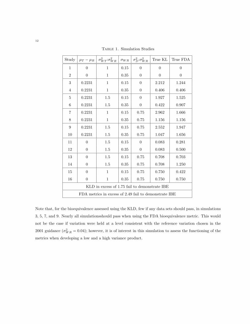
12

Table 1. Simulation Studies

Study µT − µR σ2WT :σ2

WR σWR σ2D:σ2

WR True KL True FDA

1 0 1 0.15 0 0 0

2 0 1 0.35 0 0 0

3 0.2231 1 0.15 0 2.212 1.244

4 0.2231 1 0.35 0 0.406 0.406

5 0.2231 1.5 0.15 0 1.927 1.525

6 0.2231 1.5 0.35 0 0.422 0.907

7 0.2231 1 0.15 0.75 2.962 1.666

8 0.2231 1 0.35 0.75 1.156 1.156

9 0.2231 1.5 0.15 0.75 2.552 1.947

10 0.2231 1.5 0.35 0.75 1.047 1.656

11 0 1.5 0.15 0 0.083 0.281

12 0 1.5 0.35 0 0.083 0.500

13 0 1.5 0.15 0.75 0.708 0.703

14 0 1.5 0.35 0.75 0.708 1.250

15 0 1 0.15 0.75 0.750 0.422

16 0 1 0.35 0.75 0.750 0.750

KLD in excess of 1.75 fail to demonstrate IBE

FDA metrics in excess of 2.49 fail to demonstrate IBE

Note that, for the bioequivalence assessed using the KLD, few if any data sets should pass, in simulations

3, 5, 7, and 9. Nearly all simulationsshould pass when using the FDA bioequivalence metric. This would

not be the case if variation were held at a level consistent with the reference variation chosen in the

2001 guidance (σ2WR = 0.04); however, it is of interest in this simulation to assess the functioning of the

metrics when developing a low and a high variance product.

13

Restricted Maximum Likelihood (REML) based estimation procedure.

Observations in each simulated data set were analyzed separately using a two stage (mixed effect, re-

stricted maximum likelihood) linear model including terms for sequence, period, and formulation. Subject

was specified as a random effect, and a heteroscedastic compound symmetric matrix for between-subject

variances was assumed. Point estimates were derived for the parameters of interest, and estimates were

applied to the KLD (7) and the FDA metric (5) to derive point estimates for the metrics of interest. SAS

PROC MIXED running on a UNIX machine was used to perform all calculations.

The bootstrapping method.

For each of the 100 simulated data sets in each simulation, 2000 bootstrap samples were generated

preserving the number of subjects per sequence (cf. FDA Guidance, 1997). REML based estimation

was used to derive the estimates in each bootstrap sample and to calculate the metrics of interest in

each sample. The ninety-fifth percentile of the 2000 bootstrap values is the upper bound, using the

non-parametric percentile method, for the metric of interest (see Efron and Tibshirani, Ch. 25, 1993).

For each simulation, the mean (SD) across the one-hundred simulations are tabulated as are the 5th,

25th, 50th, 75th, and 95th quantiles for the bootstrapped upper ninety-fifth quantiles for each metric to

provide a summary of the distribution of observations.

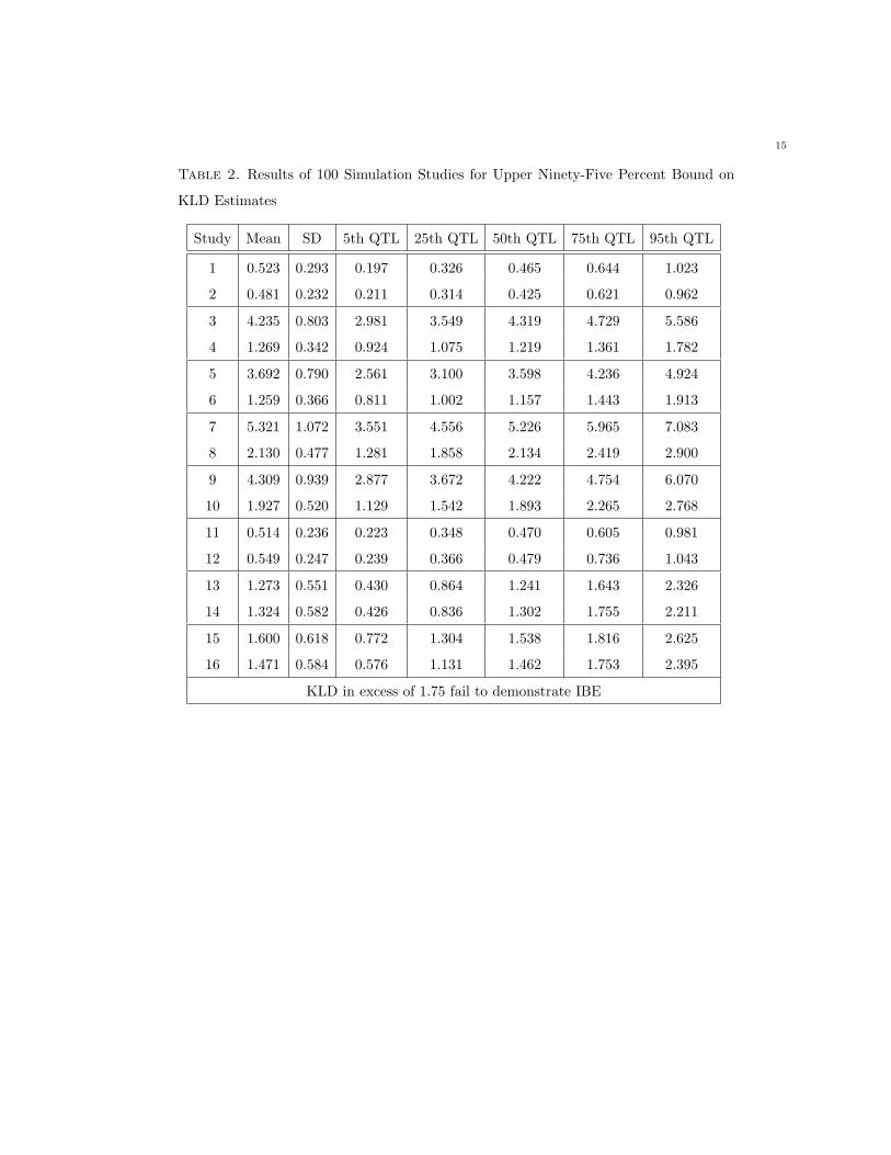
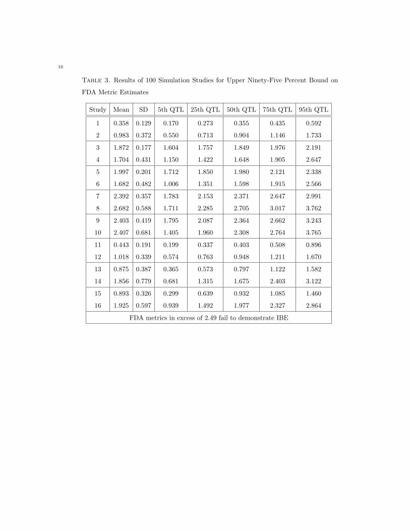
2.3. Results. Summaries of results for the KL and FDA Divergences upper 95% bound (generated using

the bootstrap) are presented in Tables 2 and 3, respectively. Simulations 1 and 2 reflect the expected

bias in the criteria under study due to the REML procedure (see also Chapter 5.1); however, note that

we would not expect this bias to impact inference for a truly bioequivalent pair of products for either

criteria.

Examining the inferential statistic for the KLD, a mean change of 20% causes an appreciable reaction for

a low variability drug product which is not as appreciable for a high variability product due to scaling

to variation (simulations 3 and 4, Table 2). In contrast, the FDA metric begins to identify individual

inequivalence for a highly variable drug product (simulation 4, Table 3) but not for a low variability drug

product (simulation 3, Table 3).

For the KLD, a 50% change in variances and a 20% change in means (simulations 5 and 6, Table 2)

causes an appreciable reaction for a low variability drug product and greater than 5% of studies fail for

a high variability product. However, the FDA criteria still indicates that formulations are bioequivalent

14

for the low variability product (simulation 5, Table 3). For the high variability product, greater than 5%

of simulations begin to fail IBE under this approach (simulation 6, Table 3).

When an appreciable σ2D is introduced with a 20% change in means (simulation 8, Table 2), greater

than 75% of studies for the highly variable drug product begin to fail bioequivalence under the KLD

approach (note that no studies pass for the low variability product, simulation 7, Table 2) while most

studies under the FDA criteria fail to demonstrate bioequivalence (simulations 7 and 8, Table 3). This

finding continues when changes in means, changes in within-subject variance, and an appreciable σ2D are

introduced in parallel (simulations 9 and 10, Tables 2 and 3).

As expected, little reaction in the upper bound of the KLD was observed when within-subject test

productvariance was increased (simulations 11 and 12, Table 2), with the introduction of an appreciable

σ2D (simulations 15 and 16, Table 2) or in the combination of the two factors (simulations 13 and 14, Table

2). However, approximately 25% of simulations fail to demonstrate bioequivalence for highly variable

products using the FDA metric in combination with an appreciable σ2D (simulations 14 and 16, Table 3).

15

Table 2. Results of 100 Simulation Studies for Upper Ninety-Five Percent Bound on

KLD Estimates

Study Mean SD 5th QTL 25th QTL 50th QTL 75th QTL 95th QTL

1 0.523 0.293 0.197 0.326 0.465 0.644 1.023

2 0.481 0.232 0.211 0.314 0.425 0.621 0.962

3 4.235 0.803 2.981 3.549 4.319 4.729 5.586

4 1.269 0.342 0.924 1.075 1.219 1.361 1.782

5 3.692 0.790 2.561 3.100 3.598 4.236 4.924

6 1.259 0.366 0.811 1.002 1.157 1.443 1.913

7 5.321 1.072 3.551 4.556 5.226 5.965 7.083

8 2.130 0.477 1.281 1.858 2.134 2.419 2.900

9 4.309 0.939 2.877 3.672 4.222 4.754 6.070

10 1.927 0.520 1.129 1.542 1.893 2.265 2.768

11 0.514 0.236 0.223 0.348 0.470 0.605 0.981

12 0.549 0.247 0.239 0.366 0.479 0.736 1.043

13 1.273 0.551 0.430 0.864 1.241 1.643 2.326

14 1.324 0.582 0.426 0.836 1.302 1.755 2.211

15 1.600 0.618 0.772 1.304 1.538 1.816 2.625

16 1.471 0.584 0.576 1.131 1.462 1.753 2.395

KLD in excess of 1.75 fail to demonstrate IBE

16

Table 3. Results of 100 Simulation Studies for Upper Ninety-Five Percent Bound on

FDA Metric Estimates

Study Mean SD 5th QTL 25th QTL 50th QTL 75th QTL 95th QTL

1 0.358 0.129 0.170 0.273 0.355 0.435 0.592

2 0.983 0.372 0.550 0.713 0.904 1.146 1.733

3 1.872 0.177 1.604 1.757 1.849 1.976 2.191

4 1.704 0.431 1.150 1.422 1.648 1.905 2.647

5 1.997 0.201 1.712 1.850 1.980 2.121 2.338

6 1.682 0.482 1.006 1.351 1.598 1.915 2.566

7 2.392 0.357 1.783 2.153 2.371 2.647 2.991

8 2.682 0.588 1.711 2.285 2.705 3.017 3.762

9 2.403 0.419 1.795 2.087 2.364 2.662 3.243

10 2.407 0.681 1.405 1.960 2.308 2.764 3.765

11 0.443 0.191 0.199 0.337 0.403 0.508 0.896

12 1.018 0.339 0.574 0.763 0.948 1.211 1.670

13 0.875 0.387 0.365 0.573 0.797 1.122 1.582

14 1.856 0.779 0.681 1.315 1.675 2.403 3.122

15 0.893 0.326 0.299 0.639 0.932 1.085 1.460

16 1.925 0.597 0.939 1.492 1.977 2.327 2.864

FDA metrics in excess of 2.49 fail to demonstrate IBE

17

2.4. Summary. Bias in Estimates for the Metrics It is known, as will be shown in Section 5, that

estimates for the FDA metric and KLD are positively biased in small samples using unbiased method-

of-moment estimation. Additionally, it is known (Endrenyi et al., 2000) that estimates from constrained

REML estimation are positively biased, contributing to even more positive bias in the estimated metrics.

Thus the positive bias observed in our simulation studies is not unexpected.

Sensitivity of Metrics to Parameter Space The KLD appears directly sensitive to changes in the means

between formulations and in the presence of subject-by-formulation interaction - directly measuring dis-

crepancy between formulations as expected. The FDA metric’s behaviour appears insensitive to some

factors; this is consistent with earlier findings (Zariffa et al., 2000). Thus conclusions of bioequivalence

may be overly dependent on the level of within-subject variation.

3. Retrospective Assessment

3.1. Data and Methods. Fifteen randomized, replicate design studies (sample size from 12 to 74) were

conducted (as described in Zariffa et al., 2000). In each study, subjects provided data on four separate

sessions separated by adequate washout to avoid residual drug concentrations from the previous occasion.

In all, subjects received each drug formulation twice over the duration of the study.

Plasma concentration-time profiles were obtained after each administration, and non-compartmental

methods were used to derive summary measures AUC (area under the curve) and Cmax (maximal con-

centration.) Six of the 15 studies involved multiple drug components (e.g. multi-product combinations,

or parent and active metabolite combinations) yielding a total of 22 data sets, each containing AUC and

Cmax. Seven data sets involved 2 sequences of formulation administration (RTRT, TRTR or RTTR,

TRRT) while the other 14 data sets involved 4 sequences (TTRR, RRTT, RTTR, TRRT), and 1 data

set had 5 sequences of treatment administration (TTRR, RRTT, RTTR, TRRT, TRTR).

These data were subjected to statistical analysis under the current average bioequivalence guidance from

FDA (1992) and under the proposed guidance for individual bioequivalence (1997) to derive estimates

for the quantities of interest.

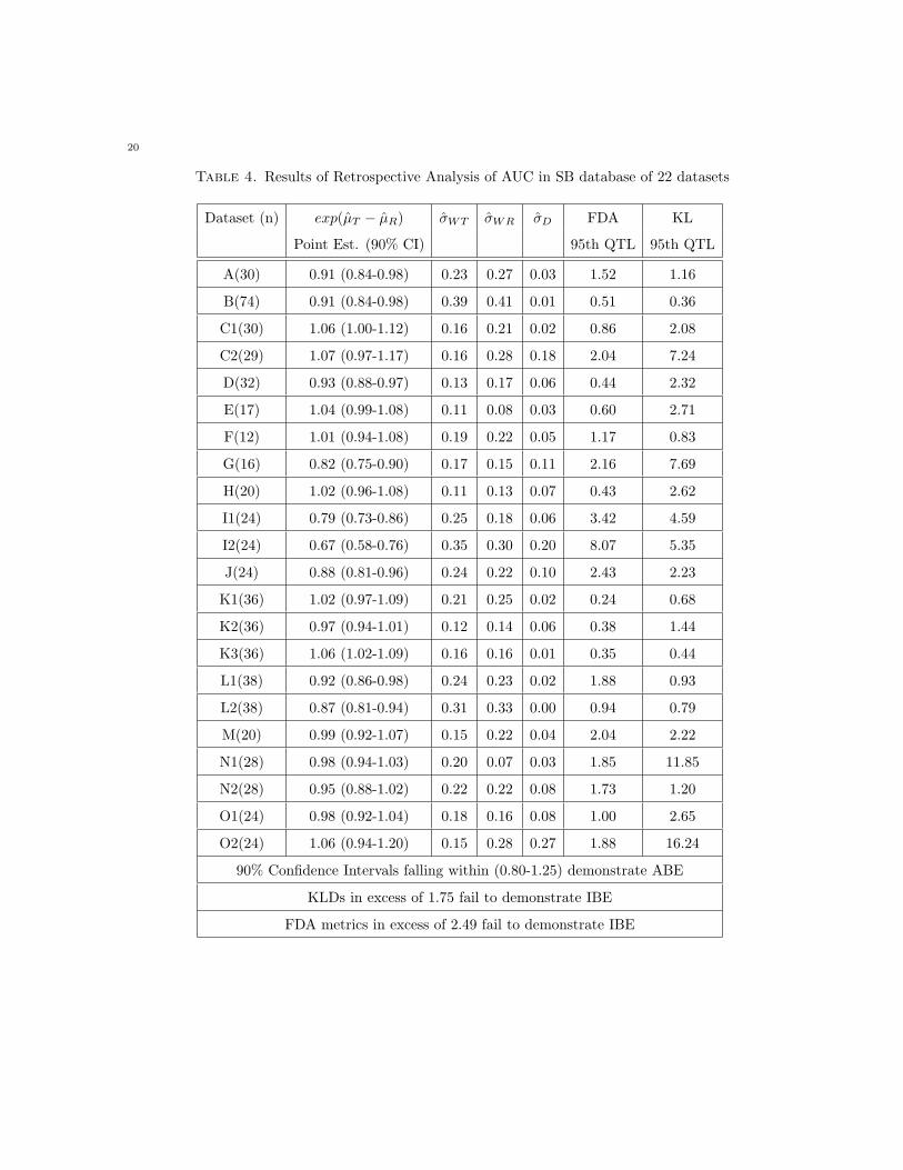
3.2. Results. Results of inference under the existing 1992 Guidance from FDA for average bioequiva-

lence, and under the proposed procedures for the FDA metric and the KLD are presented based upon

18

twenty-two SB data sets (previously published in Zariffa et al., 2000) for AUC (Table 4) and Cmax (Table

5) are presented below.

Average bioequivalence is demonstrated if the ninety-percent confidence intervals on exp(µT − µR) for

AUC and Cmax are contained within (0.80-1.25). Individual bioequivalence is concluded under the

approach described in the 1997 FDA Guidance if the 95th quantile of the bootstrap for the FDA metric

(5) is less than the value 2.49. Individual bioequivalence is concluded under the KLD approach described

in this paper if the 95th quantile of the bootstrap for the KLD (7) is less than the value 1.75.

Data sets G, I1, and I2 (Table 4) fail to demonstrate average bioequivalence for AUC, and data sets A,

F, G, I1, I2, and L2 (Table 5) fail to demonstrate average bioequivalence for Cmax. Of these, only the

Cmax data set for L2 (Table 5) demonstrates IBE using the KLD metric, while AUC data set G (Table

4) and Cmax data sets A and L2 (Table 5) demonstrate IBE using the FDA metric. Both the KLD

and FDA metric permit changes in means which are sufficiently large to fail average bioequivalence to

be ’masked’ by large within-subject variation - allowing for IBE demonstration while failing ABE. Mixed

scaling (data set G) also appears to play a role for the FDA metric. Note that the ABE procedure as

currently defined (FDA Guidance, 1992) is not the equivalent of a KLD for ABE assessment (Kullback,

1968); such a KLD in this context is sometimes referred to as ’scaled-ABE’ as the discrepancy in means is

assessed relative to within-subject variation. KLD based ABE assessment will be the subject of a future

communication.

KLD appears to be a more stringent criteria (i.e. harder to demonstrate IBE) than the FDA metric.

Individual bioequivalence is demonstrated for all AUC data sets except I1 and I2 (Table 4) based on

assessment using the FDA metric; however, using the KLD metric, we find that data sets C1, C2, D,

E, G, H, I1, I2, J, M, N1, O1, and O2 (13 of 22 data sets, Table 4) fail to demonstrate individual

bioequivalence. For data sets where average bioequivalence was not demonstrated (G, I1, and I2, Table

4), the reasoning is obvious, but failures in the other data sets are contributed to by slight changes in

means accompanied by changes in within-subject variance and/or the presence of non-negligible subject

by formulation interactions. Note that for some of these data sets (C1, C2, D, E, G, H, M, N1, O1,

and O2, Table 4) decreased within-subject variance on test formulation relative to reference and/or the

FDA mixed scaling procedure may have contributed to successful demonstration of IBE under the FDA

approach where the KLD correctly identifies a substantial difference between the characteristics of the

formulations (see in particular, AUC data sets G and O2, Table 4).

19

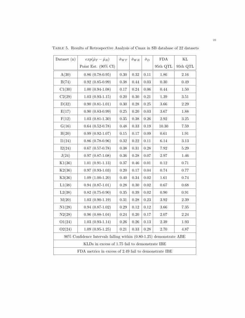
This observation is reinforced by the results for Cmax. Individual bioequivalence with respect to Cmax

is concluded for all data sets except D, E, F, G, I1, I2, J, M, N1, and O2 using the FDA metric (Table 5);

however, for Cmax, the KLD identifies only data sets B, C1, J, K1, K2, K3, L1, and L2 as meeting the

standards for individual bioequivalence (Table 5). Inference is similar between criteria for data sets D, E,

F, G, I1, I2, M, N1, and O2 (Table 5), but in the other data sets, while the KLD identifies distributional

dissimilarities as being of concern, the FDA metric passes the individual bioequivalence standard due

to decreased within-subject variance on test formulation relative to reference and/or the FDA mixed

scaling procedure. In only one case, data set J for Cmax (Table 5), was a failure for the FDA criteria

distinguished from passage under the proposed KLD method.

20

Table 4. Results of Retrospective Analysis of AUC in SB database of 22 datasets

Dataset (n) exp(µT − µR) σWT σWR σD FDA KL

Point Est. (90% CI) 95th QTL 95th QTL

A(30) 0.91 (0.84-0.98) 0.23 0.27 0.03 1.52 1.16

B(74) 0.91 (0.84-0.98) 0.39 0.41 0.01 0.51 0.36

C1(30) 1.06 (1.00-1.12) 0.16 0.21 0.02 0.86 2.08

C2(29) 1.07 (0.97-1.17) 0.16 0.28 0.18 2.04 7.24

D(32) 0.93 (0.88-0.97) 0.13 0.17 0.06 0.44 2.32

E(17) 1.04 (0.99-1.08) 0.11 0.08 0.03 0.60 2.71

F(12) 1.01 (0.94-1.08) 0.19 0.22 0.05 1.17 0.83

G(16) 0.82 (0.75-0.90) 0.17 0.15 0.11 2.16 7.69

H(20) 1.02 (0.96-1.08) 0.11 0.13 0.07 0.43 2.62

I1(24) 0.79 (0.73-0.86) 0.25 0.18 0.06 3.42 4.59

I2(24) 0.67 (0.58-0.76) 0.35 0.30 0.20 8.07 5.35

J(24) 0.88 (0.81-0.96) 0.24 0.22 0.10 2.43 2.23

K1(36) 1.02 (0.97-1.09) 0.21 0.25 0.02 0.24 0.68

K2(36) 0.97 (0.94-1.01) 0.12 0.14 0.06 0.38 1.44

K3(36) 1.06 (1.02-1.09) 0.16 0.16 0.01 0.35 0.44

L1(38) 0.92 (0.86-0.98) 0.24 0.23 0.02 1.88 0.93

L2(38) 0.87 (0.81-0.94) 0.31 0.33 0.00 0.94 0.79

M(20) 0.99 (0.92-1.07) 0.15 0.22 0.04 2.04 2.22

N1(28) 0.98 (0.94-1.03) 0.20 0.07 0.03 1.85 11.85

N2(28) 0.95 (0.88-1.02) 0.22 0.22 0.08 1.73 1.20

O1(24) 0.98 (0.92-1.04) 0.18 0.16 0.08 1.00 2.65

O2(24) 1.06 (0.94-1.20) 0.15 0.28 0.27 1.88 16.24

90% Confidence Intervals falling within (0.80-1.25) demonstrate ABE

KLDs in excess of 1.75 fail to demonstrate IBE

FDA metrics in excess of 2.49 fail to demonstrate IBE

21

Table 5. Results of Retrospective Analysis of Cmax in SB database of 22 datasets

Dataset (n) exp(µT − µR) σWT σWR σD FDA KL

Point Est. (90% CI) 95th QTL 95th QTL

A(30) 0.86 (0.78-0.95) 0.30 0.32 0.11 1.86 2.16

B(74) 0.92 (0.85-0.99) 0.38 0.44 0.03 0.30 0.49

C1(30) 1.00 (0.94-1.08) 0.17 0.24 0.06 0.44 1.50

C2(29) 1.03 (0.93-1.15) 0.20 0.30 0.21 1.39 3.51

D(32) 0.90 (0.81-1.01) 0.30 0.28 0.25 3.66 2.29

E(17) 0.90 (0.83-0.99) 0.25 0.20 0.03 3.67 1.88

F(12) 1.03 (0.81-1.30) 0.35 0.38 0.26 2.92 3.25

G(16) 0.64 (0.52-0.78) 0.48 0.33 0.19 10.30 7.59

H(20) 0.99 (0.92-1.07) 0.15 0.17 0.09 0.61 1.91

I1(24) 0.86 (0.78-0.96) 0.32 0.22 0.11 6.14 3.13

I2(24) 0.67 (0.57-0.78) 0.38 0.31 0.28 7.92 5.29

J(24) 0.97 (0.87-1.08) 0.36 0.28 0.07 2.97 1.46

K1(36) 1.01 (0.91-1.13) 0.37 0.46 0.01 0.12 0.71

K2(36) 0.97 (0.93-1.03) 0.20 0.17 0.04 0.74 0.77

K3(36) 1.09 (1.00-1.20) 0.40 0.34 0.02 1.61 0.74

L1(38) 0.94 (0.87-1.01) 0.28 0.30 0.02 0.67 0.68

L2(38) 0.82 (0.75-0.90) 0.35 0.39 0.02 0.90 0.91

M(20) 1.03 (0.90-1.19) 0.31 0.28 0.23 3.92 2.39

N1(28) 0.94 (0.87-1.02) 0.29 0.12 0.12 3.66 7.35

N2(28) 0.96 (0.88-1.04) 0.24 0.20 0.17 2.07 2.24

O1(24) 1.03 (0.93-1.14) 0.26 0.26 0.13 2.39 1.93

O2(24) 1.09 (0.95-1.25) 0.21 0.33 0.28 2.70 4.87

90% Confidence Intervals falling within (0.80-1.25) demonstrate ABE

KLDs in excess of 1.75 fail to demonstrate IBE

FDA metrics in excess of 2.49 fail to demonstrate IBE

22

3.3. Summary. As expected based on the simulations previously presented and confirmed in the existing

data sets, the FDA metric by chance finds slight increase in within-subject test variance unacceptable in

the coincident presence of a small subject-by-formulation interaction and in the presence of changes in

means between formulations. The KLD assesses these slight changes relative to the overall background

noise (as measured by the within-subject variances for test and reference formulations).

The KLD rejects individual bioequivalence for a greater number of data sets than the FDA metric. The

problems with inference (observed mean/variance tradeoffs) previously identified for the FDA metric do

not appear as prevalent with inference using the KLD, and overall, inference using the KLD appears

more consistent with a procedure which would be expected to be an extension of average bioequivalence.

4. Discussion

Goalposts have been set based on a within-subject reference variance of 0.04. In the knowledge that the

variance of subject-by-formulation interaction increases with increasing within-subject variance (Zariffa

and Patterson, 2000b) and is ill-characterized statistically in studies of this size (Zariffa et al., 2000),

the definition of this goalpost incorporates the idea that it should be scaled to within-subject reference

variation as part of the aggregate criteria; however, the level set (σ2D/σ2

WR=0.75) seems arbitrary and

should be justified for all drugs under consideration. While the historical precedent for arbitrary setting

of the allowable mean difference at twenty percent is not clear, it has withstood the test of time in

protecting the public health (Barrett et al., 2000). There is little evidence available to suggest that the

same arbitrary limit of 0.75 for subject-by-formulation interaction will protect the public health; indeed,

it could limit market access for many drugs (e.g. highly variable drugs) for which levels in excess of this

arbitrary value are appropriate. Market access should not be allowed using procedures under study for

this very reason.

The KLD as a measure of individual bioequivalence seems to identify more data sets as being of concern

than the proposed FDA metric. This appears to be due to the ability of the FDA metric to reward novel

formulations for which the within-subject variance is decreased relative to the reference product and the

use of the mixed scaling procedure. While the KLD may be viewed as being a more ’stringent’ criteria

than the FDA metric, it appears to be mathematically tractable and to identify those data sets where

changes in formulation are of particular concern.

23

The KLD is a viable alternative to the FDA proposed procedure for the assessment of individual bioequiv-

alence. It appear to be sensitive to changes in mean response between formulations and to the detection

of subject-by-formulation interaction - a desirable property for a metric. Identification of differences

between individual responses to formulation are identified clearly in low variability drug products, and

bigger quantitative differences must be observed before the KLD flags them as being important for high

variability products - another desirable property.

Formulations are not ’rewarded’ for being less variable when using the KLD while they frequently are

when using the FDA metric (Zariffa et al., 2000). Coincident differences in average bioavailability with

decreased variance for the test formulation may thus allow for market access under the proposed FDA

metric (Barrett et al., 2000) and could happen in practice (Zariffa et al., 2000). Failure of continued

efficacy or undesirable side effects could be observed as a result of such a situation. Use of a criteria such

as the KLD which does not allow for such a ’trade-off’ is a desirable property in a global marketplace

where regulators cannot guarantee that patients will not be switched back and forth from the reference

and test products on a daily, weekly, or monthly basis when their prescription is filled at the pharmacist,

and formulations are switched to the least expensive product available in stock. International Regulators

cannot at present ensure that all patients will be switched to the new formulation cosistently, immediately,

and permanently. Use of metrics such as that proposed by FDA may place patient populations at increased

risk of side-effects or ineffective switching due to marketplace forces beyond regulatory control.

Another benefit of the KLD metric is that it potentially does not require the use of a replicate design

to assess individual bioequivalence. The divergence can be computed based upon any crossover design.

Previous work by other authors (Gould, 2000) reported similar results for different metrics; however, it

is known that the approach proposed by Gould (2000) does not perform well for highly variable drug

products (data on file). As such highly variable products are the primary compounds for which data

will be collected under the final FDA guidance (2000), viable alternative procedures should be sought.

Further work will investigate whether the conclusions with regard to IBE based on reduced level designs

(i.e. normal two period crossovers) are the same as those based upon replicate type designs for the KLD.

The KLD might also be extended to assess the divergence between two individual PK profiles, eliminating

the need for summary measures such as AUC and Cmax.

Additionally, the KLD fulfills the requirements of a true discrepancy measure, and while it may not at

first glance be as readily interpretable by clinicians as the FDA proposed metric, the definition of the

Divergence follows strict scientific, mathematical rules based on well established methods of information,

24

sufficiency, and distributional theory which can be directly mathematically justified to a clinical audience

and are acceptable statistically.

Practical issues, however, could impact upon the use of this discrepancy metric in clinical studies. In

particular, the property of the KLD related to dividing by test product variation (ie. by σ2WT ) may not

be acceptable in practice as an argument can be made that by producing a highly variable test product,

the denominator will become large, thus decreasing the discrepancy measured and observed. However, it

should be noted that in such a case, we would also expect the term for σ2W T

σ2W R

to become larger, offsetting

any ’decreases’ in the magnitude of other terms in the discrepancy measure. Simulation studies will be

conducted to characterise the type one and two error properties of the KLD under such circumstances to

determine if performance of the discrepancy measure in such circumstances is of concern.

The FDA metric’s properties appear less desirable. The well established ability (Endrenyi and Hao,

1998; Zariffa et al., 2000, and Zariffa and Patterson, 2001) of the FDA metric to reward less variable

formulations appears particularly concerning as marketplace forces can not be guaranteed to safeguard

patients switching from test formulation back to reference.

In conclusion, the results of simulation and retrospective analysis to date indicate that the KLD metric

is a viable alternative to the FDA-proposed metric and that its mathematical properties as a Diver-

gence measurement make it a more readily interpretable measure of the individual differences between

formulations.

5. Extensions

5.1. Bias in Plug-In Estimates for KLD and FDA Metric. The further consideration of bias of the

’plug-in’ estimates for the FDA and KL criteria will be based on the estimation procedures developed by

Chinchilli and Esinhart (1996) and described in application in this setting by Hyslop et al. (2000). The

estimators are used as it is known (Endrenyi et al., 2000) that current REML based estimators for σD are

positively biased when estimates are near zero, though in practical applications little discernable impact

on inference for this finding has been noted (Hauck et al., 2000). We begin by establishing pairwise

independence of the method-of-moments estimators.

Theorem 5.1. Pairwise Independence of Method-of-Moment Estimators

25

In a balanced, replicate, crossover design, with no missing data, unbiased method of moment estimators

δ, MI , MT , and MR for δ = µT − µR, σ2I = σ2

D + σ2W T +σ2

W R

2 , σ2WT , and σ2

WR are pairwise independent.

Proof: Let the loge-transformed AUC or Cmax be represented by ytijk be the k-th response (k = 1, 2)

for the j-th subject administered treatment t (t = T,R) in sequence i (i = 1, . . . , s). Let the individual

difference across formulations be denoted Iij = yTij• − yRij• such that

δ =1s

s∑i=1

[ 1ni

ni∑j=1

Iij

]and

MI =1

(∑s

i=1 ni)− s

s∑i=1

ni∑j=1

(Iij − Ii)2

It follows that these two statistics δ and MI are independent based on previous results attributed to

Fisher (described in Johnson et al., Vol 2, 1995 and Muirhead, 1982). Vonesh and Chinchilli (1997) show

that δ is unbiased for δ, and Chinchilli and Esinhart (1996) showed that MI ∼ σ2Iχ2

ν/ν where ν is the

degrees of freedom associated with MI , ν = (∑s

i=1 ni)− s = n− 2.

Let the individual difference within formulations for test and reference formulations be denoted

Tij = yTij1 − yTij2 and Rij = yRij1 − yRij2, respectively. Within-subject variances are estimated by

MT =1

2((∑s

i=1 ni)− s)

s∑i=1

ni∑j=1

(Tij − T i)2

and

MR =1

2((∑s

i=1 ni)− s)

s∑i=1

ni∑j=1

(Rij −Ri)2

Chinchilli and Esinhart (1996) showed that MT ∼ σ2WT χ2

ν/ν where ν is the degrees of freedom associated

with MT , and MR ∼ σ2WRχ2

ν/ν where ν is the degrees of freedom associated with MR. As MR and MT

are derived from independent multivariate normal observations, MR and MT are independent under (4).

It remains to show that the estimates of within-subject variability (MR and MT ) are pairwise independent

with δ and MI . Here we refer the reader to the well known result attributed to Altman and Bland (1983)

based on the properties of the multivariate normal density such that if A and B are bivariate normally

distributed with non-null correlation ρ and homogeneous variance then A+B2 and A−B are independent

using the well-known properties of the multivariate normal distribution (Bickel and Doksum, 1977). In

26

this context, it follows that Rij , Tij , and Iij are mutually independent, and as subjects are independent,

it follows that MR is independent of MI and δ, and MT is independent of MI and δ.���

We now turn to discussion of the properties of the ’plug-in’ metrics themselves in balanced, replicate,

crossover designs, with no missing data. The ’plug-in’ method-of-moments estimate for the FDA metric

for IBE is consistent and asymptotically unbiased, and an unbiased small sample estimator can be derived.

Theorem 5.2. Bias in FDA Metric

The FDA metric (5) may be estimated (FDA Guidance, 1997, 1999a, 1999b, 2000, 2001) using the

method of moments approach as:

δ2 + MI + MT

2 − 3MR

2

MR=

δ2

MR+

MI

MR+

(12

)(MT

MR

)− 3

2(8)

This statistic is a consistent estimator and furthermore is asymptotically unbiased and positively biased

in small samples with expected value

ν

ν − 2

( δ2

σ2WR

+(n + 1)σ2

I

nσ2WR

+σ2

WT

2σ2WR

)− 3

2(9)

Proof: Let (4) and Theorem 5.1 with corresponding assumptions hold. Then it follows directly that δ2

σ2I /n

∼

χ2′

1 ( δ2

σ2I /n

) (Vonesh and Chinchilli, 1997) where χ2′

1 represents a non-central chi-squared distribution with

one degree of freedom and non-centrality parameter δ2

σ2I /n

(Muirhead, p22, 1982). As (8) is an estimate for

(5) obtained from method of moments and (5) is continuous, then (8) is consistent (Bickel and Doksum,

1977).

Taking the expectation of terms in (8) and assuming terms are pairwise independent under Theorem 2.1,

E( δ2

MR+

MI

MR+

(12

)(MT

MR

)− 3

2

)

= E( σ2

I

n ( δ2

σ2I /n

)

σ2WR( MR

σ2W R

)

)+ E

( σ2I (MI

σ2I

)

σ2WR( MR

σ2W R

)

)+ E

( σ2WT ( MT

σ2W T

)

2σ2WR( MR

σ2W R

)

)− 3

2

Further, using the results of Muirhead (p 24, 1982), it is seen that this expression reduces to,

E( σ2

I

nσ2WR

F ′1

)+ E

( σ2I

σ2WR

F1

)+ E

( σ2WT

2σ2WR

F2

)− 3

2

where F ′i is a random variable with non-central F -distribution with non-centrality parameter δ2

σ2I /n

and

1, ν degrees of freedom. Fi is a random variable distributed according to the central-F -distribution with

27

ν, ν degrees of freedom. Taking the expectation (Muirhead, p 25 1982), we see that the result is (9). As

sample size increases,

limn→∞

[ ν

ν − 2

( δ2

σ2WR

+(n + 1)σ2

I

nσ2WR

+σ2

WT

2σ2WR

)− 3

2

]=

δ2

σ2WR

+σ2

I

σ2WR

+σ2

WT

2σ2WR

− 32

which is an unbiased estimate for (5). However in small samples, the bias is( ν

ν − 2− 1

) δ2

σ2WR

+(ν(n + 1)

n(ν − 2)− 1

) σ2I

σ2WR

+( ν

ν − 2− 1

) σ2WT

2σ2WR

≥ 0

���

We now derive an unbiased estimator for the FDA metric in small samples.

Theorem 5.3. An Unbiased FDA Metric for IBE

The FDA metric (5) may be estimated in an unbiased fashion in small samples using the method of

moments approach as:ν − 2

ν

[ δ2

MR+

(n− 1)MI

nMR+

(12

)(MT

MR

)]− 3

2(10)

Proof: Let (4) and Theorem 5.1 with corresponding assumptions hold. Taking the expectation of terms in

(10) and assuming terms are pairwise independent under Theorem 2.1 and using the results of Muirhead

(p 24, 1982), it is seen that this expression reduces to,

E( (ν − 2)σ2

I

ν(nσ2WR)

F ′1

)+ E

( (ν − 2)(n− 1)σ2I

nνσ2WR

F1

)+ E

( (ν − 2)σ2WT

2νσ2WR

F2

)− 3

2

where F ′i and Fi are random variables with the non-central and central-F -distributions as previously.

Taking the expectation (Muirhead, p 25 1982), we see that the result is

δ2

σ2WR

+σ2

I

σ2WR

+σ2

WT

2σ2WR

− 32

which is unbiased for the FDA metric (5). ���

Similarly, it is then easy to show that the ’plug-in’ method-of-moments estimate for the KLD of IBE is

consistent and asymptotically unbiased and to derive an unbiased, small sample estimate.

Theorem 5.4. Bias in the KLD for IBE

A method of moments estimator for the KLD is

12

(δ2 + MI +

MT

2+

MR

2

)( 1MR

+1

MT

)− 2 (11)

28

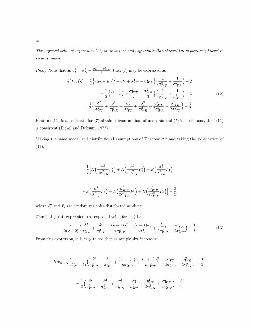
The expected value of expression (11) is consistent and asymptotically unbiased but is positively biased in

small samples.

Proof: Note that as σ2I = σ2

D + σ2W T +σ2

W R

2 , then (7) may be expressed as

d(fT , fR) =12

{(µT − µR)2 + σ2

D + σ2WT + σ2

WR

}( 1σ2

WT

+1

σ2WR

)− 2

=12

{δ2 + σ2

I +σ2

WT

2+

σ2WR

2

}( 1σ2

WT

+1

σ2WR

)− 2

=12

{ δ2

σ2WT

+δ2

σ2WR

+σ2

I

σ2WT

+σ2

I

σ2WR

+σ2

WT

2σ2WR

+σ2

WR

2σ2WT

}− 3

2

(12)

First, as (11) is an estimate for (7) obtained from method of moments and (7) is continuous, then (11)

is consistent (Bickel and Doksum, 1977).

Making the same model and distributional assumptions of Theorem 2.2 and taking the expectation of

(11),

12

[E

( σ2I

nσ2WR

F ′1

)+ E

( σ2I

nσ2WT

F ′2

)+ E

( σ2I

σ2WR

F1

)

+E( σ2

I

σ2WT

F2

)+ E

( σ2WT

2σ2WR

F3

)+ E

( σ2WR

2σ2WT

F4

)]− 3

2

where F ′i and Fi are random variables distributed as above.

Completing this expression, the expected value for (11) is:

ν

2(ν − 2)

( δ2

σ2WR

+δ2

σ2WT

+(n + 1)σ2

I

nσ2WR

+(n + 1)σ2

I

nσ2WT

+σ2

WT

2σ2WR

+σ2

WR

2σ2WT

)− 3

2(13)

From this expression, it is easy to see that as sample size increases:

limn→∞

[ ν

2(ν − 2)

( δ2

σ2WR

+δ2

σ2WT

+(n + 1)σ2

I

nσ2WR

+(n + 1)σ2

I

nσ2WT

+σ2

WT

2σ2WR

+σ2

WR

2σ2WT

)− 3

2

]

=12

( δ2

σ2WR

+δ2

σ2WT

+σ2

I

σ2WR

+σ2

I

σ2WT

+σ2

WT

2σ2WR

+σ2

WR

2σ2WT

)− 3

2

29

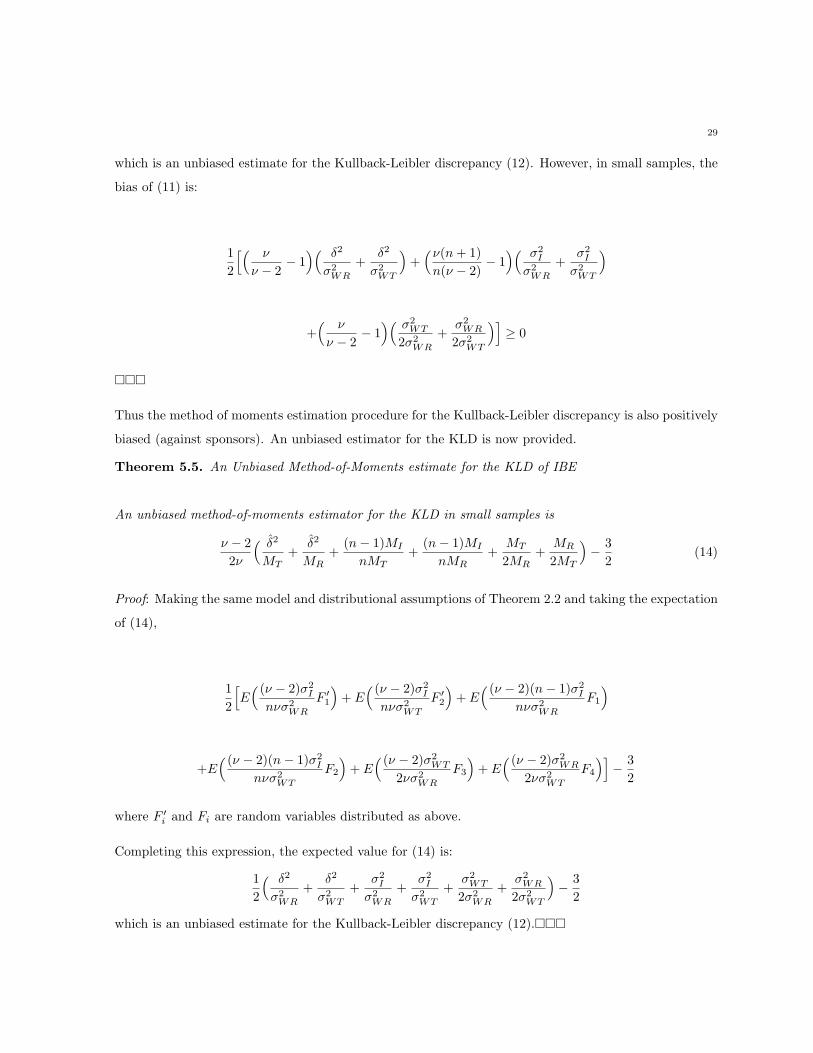
which is an unbiased estimate for the Kullback-Leibler discrepancy (12). However, in small samples, the

bias of (11) is:

12

[( ν

ν − 2− 1

)( δ2

σ2WR

+δ2

σ2WT

)+

(ν(n + 1)n(ν − 2)

− 1)( σ2

I

σ2WR

+σ2

I

σ2WT

)

+( ν

ν − 2− 1

)( σ2WT

2σ2WR

+σ2

WR

2σ2WT

)]≥ 0

���

Thus the method of moments estimation procedure for the Kullback-Leibler discrepancy is also positively

biased (against sponsors). An unbiased estimator for the KLD is now provided.

Theorem 5.5. An Unbiased Method-of-Moments estimate for the KLD of IBE

An unbiased method-of-moments estimator for the KLD in small samples is

ν − 22ν

( δ2

MT+

δ2

MR+

(n− 1)MI

nMT+

(n− 1)MI

nMR+

MT

2MR+

MR

2MT

)− 3

2(14)

Proof: Making the same model and distributional assumptions of Theorem 2.2 and taking the expectation

of (14),

12

[E

( (ν − 2)σ2I

nνσ2WR

F ′1

)+ E

( (ν − 2)σ2I

nνσ2WT

F ′2

)+ E

( (ν − 2)(n− 1)σ2I

nνσ2WR

F1

)

+E( (ν − 2)(n− 1)σ2

I

nνσ2WT

F2

)+ E

( (ν − 2)σ2WT

2νσ2WR

F3

)+ E

( (ν − 2)σ2WR

2νσ2WT

F4

)]− 3

2

where F ′i and Fi are random variables distributed as above.

Completing this expression, the expected value for (14) is:

12

( δ2

σ2WR

+δ2

σ2WT

+σ2

I

σ2WR

+σ2

I

σ2WT

+σ2

WT

2σ2WR

+σ2

WR

2σ2WT

)− 3

2

which is an unbiased estimate for the Kullback-Leibler discrepancy (12).���

30

Thus to conclude, both ’plug-in’ estimators are positively biased for the true KLD and FDA metrics,

respectively, under the proposed estimation method (against sponsors). Unbiased estimators may easily

be derived in balanced, complete data sets. Future research will characterise whether the positive bias

is of practical significance in PBE and IBE assessment in such data sets. Estimates from a REML

model may be utilised in construction of the metric of interest in similar fashion to that used for the

method-of-moments procedure to estimate the metrics of interest in an unbalanced or incomplete data

set. However, the estimators are known to be only asymptotically unbiased. Future simulation based

research will explore the small sample properites of such PBE and IBE REML based procedures for the

FDA metric and KLD.

Also of intuitive appeal is the consideration of multivariate statistical assessment in this setting as it

would be expected that AUC and Cmax are positively correlated. Such a multivariate approach is easily

accommodated in the KL Divergence (Dragalin and Fedorov, 1999) but is not readily tractable under the

FDA’s approach to inference.

5.2. Exploratory Activities. Further developments regarding the KLD are necessary before it could

be readily implemented in an industry setting. The use of the bootstrap appears to be unacceptable

based on feedback in practice (Montreal, AAPS/FDA Workshop, August/September 1999); thus, an

approximate procedure akin to the Cornish-Fisher technique recommended in the 1999 FDA Guidance

could be developed for the KLD based on the work by Box (1954), Ruben (1962), Cox and Hinkley (1974),

Farebrother (1990), Johnson et al., (1993), and Hyslop et al. (2000). Type 1 error rates and power

and sample requirements would also be defined, and a thorough exploration of whether it is necessary

to conduct a full replicate design in order to assess individual bioequivalence should be satisfactorily

concluded.

Acknowledgements. The authors wish to gratefully acknowledge the contributions and advice of

Stephen Senn, Henry Wynn, Nevine Zariffa, Walter Hauck, and the PhRMA Expert Panel on Bioequiv-

alence in motivating some aspects of the work which has been performed in this paper.

References

[1] Anderson, S. (1993). Individual bioequivalence: a problem of switchability (with discussion). Biopharmaceutical

Reports. 2, 1–11.

31

[2] Anderson, S. and Hauck, W.W. (1983). A new procedure for testing equivalence in bioavailability and other clinical

trials. Comm. Statist. Theory Methods, 12, 2663–2692.

[3] Anderson, S. and Hauck, W.W. (1990). Consideration of individual bioequivalence. Journal of Pharmacokinetics

and Biopharmaceutics, 18, 259–273.

[4] Barrett, J.S., Batra, V., Chow, A., Cook, J., Gould, A.L., Heller, A., Lo, MW., Patterson, S.D., Smith, B.P., Stritar,

J.A., Vega, J.M., Zariffa, N. (2000) PhRMA Perspective on Population and Individual Bioequivalence and Update

to the PhRMA Perspective on Population and Individual Bioequivalence. J Clin Pharmacol, 40, 561–575.

[5] Bickel, P.J., Doksum, K.A. (1977) Mathematical Statistics. Holden Day, SF.

[6] Box, G.E.P. (1954). Some theorems on quadratic forms applied in the study of analysis of variance problems, I.

Effect of inequality of variance in the one-way classification. em Ann. of Math. Statistics, 25, 290–302.

[7] Chinchilli, V.M., Esinhart, J.D. (1996) Design and analysis of intra-subject variability in cross-over experiments.

Statistics in Medicine, 15, 1619–1634.

[8] Colburn, W.A., Keefe, D.L. (2000) Bioavailability and Bioequivalence: Average, Population, and/or Individual. J

Clin Pharmacol, 40, 559–600.

[9] Cox, D.R. and Hinkley, D.V. (1974). Theoretical Statistics. Chapman Hall/CRC, New York.

[10] Dragalin, V. and Fedorov, V. (1999) Kullback–Leibler distance for evaluating bioequivalence: I. Criteria and Methods

Beecham Pharmaceutials Technical Report TR 1999-03.

[11] Efron, B., Tibshirani, R.J. (1993) An Introduction to the Bootstrap. Chapman and Hall, NY.

[12] Ekbohm, G., Melander, H. (1989) The subject-by-formulation interaction as a criterion of interchangeability of drugs.

Biometrics, 45, 1249–1254.

[13] Endrenyi, L. and Hao, Y. (1998). Asymmetry of the mean-variability tradeoff raises questions about the model

investigations of individual bioequivalence. International Journal of Clinical Pharmacology and Therapeutics, 36,

450–457.

[14] Endrenyi, L., Taback, N., Tothfalusi, L. (2000) Properties of the Estimated Variance Component for Subject-by-

formulation interaction in Studies of Individual Bioequivalence. Statistics in Medicine, 19, 2867–2878.

[15] Endrenyi, L. and Tothfalusi, L. (1999). Subject-by-formulation interaction in determinations of individual bioequiv-

alence: bias and prevalence. Pharm. Res., 16, 186–190.

[16] Farebrother, R.W. (1990). Algorithm AS 256. The distribution of a quadratic form in normal variables. Applied

Statistics, 39, 294–309.

[17] FDA Guidance. (1992) Statistical procedures for bioequivalence studies using a standard two treatment crossover

design.

[18] FDA Preliminary Draft Guidance. (1997) In vivo bioequivalence studies based on population and individual bioe-

quivalence approaches.

[19] FDA Draft Guidance. (1999a) BA and BE Studies for Orally Administered Drug Products: General Considerations.

[20] FDA Draft Guidance. (1999b) Average, Population, and Individual Approaches to Establishing Bioequivalence.

[21] FDA Guidance. (2000) Bioavailability and Bioequivalence Studies for Orally Administered Drug Products: General

Considerations.

[22] FDA Guidance. (2001) Statistical Approaches to Establishing Bioequivalence.

32

[23] Gould, A.L. (2000) A practical approach for evaluating population and individual bioequivalence. Statistics in

Medicine, 19, 2721–2740.

[24] Hauck, W.W., Hyslop, T., Anderson, S., Bois, F.Y., Tozer, T.N. (1995) Statistical and regulatory considerations for

multiple measures in bioequivalence testing. Clin Res Reg Affairs, 12, 249–265.

[25] Hauck, W.W., Hyslop, T., Chen, M.L., Patnaik, R., Williams, R.L., and the FDA Population/Individual Bioequiv-

alence Working Group. (2000) Subject-by-Formulation Interaction in Bioequivalence: Conceptual and Statistical

Issues. Pharmaceutical Research, 17, 375–380.

[26] Hyslop, T., Hsuan, F., Holder, D.J. (2000) A small sample confidence interval approach to assess individual bioe-

quivalence. Statistics in Medicine, 19, 2885–2897.

[27] Jeffreys, H. (1946). An invariant form for the prior probability in estimation pro. Proc. Roy. Soc. London, A, 186,

453–461.

[28] Johnson, N.L., Kotz, S. and Kemp, A.W. (1993). Univariate Discrete Distributions. 2nd ed, Wiley, New York.

[29] Jones, B., Kenward M.G. (1989) Design and Analysis of Crossover Trials. Chapman and Hall, London.

[30] Kullback, S. (1968) Information Theory and Statistics. Dover Publications, NY.

[31] Muirhead, R.J. (1982) Aspects of Multivariate Statistical Theory. John Wiley and Sons, NY.

[32] Patterson, H.D., Thompson, R. (1971) Recovery of Inter-block information when block sizes are unequal. Biometrika,

58, 545–554.

[33] Patterson, S.D., Zariffa, N.M–D. (2000) Poster presentation: Case studies in the measurement of agreement between

regimens in crossover studies. Annual Meeting of the American Society of Clinical Pharmacology and Therapeutics.

[34] Patterson, S. (2001a) A Review of the Development of Biostatistical Design and Analysis Techniques for Assessing

In Vivo Bioequivalence, Part 1. Indian Journal of Pharmaceutical Sciences, 63, 81–100.

[35] Patterson, S. (2001b) A Review of the Development of Biostatistical Design and Analysis Techniques for Assessing

In Vivo Bioequivalence, Part 2. Indian Journal of Pharmaceutical Sciences, 63, 169–186.

[36] Ruben, H. (1962) Probability content of regions under spherical normal distributions, IV: The distribution of ho-

mogenious and non-homogenious quadratic functions of normal variables. Ann. Math. Statistics, 33, 542–570.

[37] Schuirmann, D.J. (1987) A comparison of the two one-sided tests procedure and the power approach for assessing

the equivalence of average bioavailability. Journal of Pharmacokinetics and Biopharmaceutics, 15, 657–680.

[38] Senn, S. (1993) Crossover Trials in Clinical Research. John Wiley and Sons, NY.

[39] Senn, SJ. (2000) Consensus and controversy in pharmaceutical statistics (with discussion). The Statistician, 49,

135-176.

[40] Shao, J., Chow, S-C., Wang, B. (2000a) The bootstrap procedure in individual bioequivalence. Statistics in Medicine,

19, 2741–2754.

[41] Shao, J., Kubler, J., Pigeot, I. (2000b) Consistency of the bootstrap procedure in individual bioequivalence.

Biometrika, 87, 573–585.

[42] Vonesh, E.F., Chinchilli, V.M. (1997) Linear and Nonlinear models for the analysis of repeated measurements. Marcel

Dekker, NY.

[43] Westlake, W.J. (1986) Bioavailability and bioequivalence of pharmaceutical formulations. Biopharmaceutical Statis-

tics for Drug Development, K. Peace, ed. Marcel Dekker, NY, 329–352.

33

[44] Zariffa, N.M–D., Patterson, S.D., Boyle, D., Hyneck, H. (2000) Case Studies, Practical Issues, and Observations on

Population and Individual Bioequivalence. Statistics in Medicine, 19, 2811–2820.

[45] Zariffa, N.M–D., Patterson, S.D. (2001) Population and Individual Bioequivalence: Lessons from Real Data and

Simulation Studies. J Clin Pharmacol, 41, 811–822.