evaluating image retrieval

EVALUATING IMAGE RETRIEVAL

by

Nikhil Vasudev Shirahatti

Submitted for Approval: 27/04/2005

Thesis

submitted in partial fulfillment of

the requirements of the Degree of

Master of Science in

Electrical and Computer Engineering.

University of Arizona

May 2005

c© Nikhil V. Shirahatti, 2005

ii

This thesis by Nikhil V. Shirahatti

is accepted in its present form by the

Department of Electrical and Computer Engineering

as satisfying the thesis requirements for the Degree of

Master of Science.

Approved by the Thesis Supervisor

Dr. Kobus Barnard Date

Approved by Co-advisor

Dr. Robin Strickland Date

ii

I, Nikhil V. Shirahatti, hereby grant permission to the University Librarian at Uni-versity of Arizona to provide copies of the thesis, on request, on a non-profit basis.

Signature of Author

Signature of Supervisor

Signature of Co-Advisor

iii

Acknowledgements

I would like to thank Prof. Kobus Barnard who, as my advisor helped me understand

the problem and guided me in my efforts to solve this benchmarking bugaboo. It

is the result of our team work that we have a working model of an image retrieval

evaluation system. My regards also to Prof. Robin Strickland for giving valuable

hints in presentation and documentation of this research work. Kudos to all the

participants who have helped me collect an appreciable amount of data. Also, many

thanks to Prof. Nicholas Heard for providing with the source code for a bayesian

approach to curve fitting.

iv

Table of Contents

Acknowledgements iv

Table of Contents v

List of Tables vii

List of Figures viii

Abstract x

Chapter 1. Introduction 1

1.1 Image Retrieval Systems . . . . . . . . . . . . . . . . . . . . . . . . . . . . . . . . . . . . . . . . . . . . . . 41.2 Previous work . . . . . . . . . . . . . . . . . . . . . . . . . . . . . . . . . . . . . . . . . . . . . . . . . . . . . . . . 91.3 Thesis organization . . . . . . . . . . . . . . . . . . . . . . . . . . . . . . . . . . . . . . . . . . . . . . . . . . 11

Chapter 2. Developing a Reference Data Set 12

2.1 Experimental setup . . . . . . . . . . . . . . . . . . . . . . . . . . . . . . . . . . . . . . . . . . . . . . . . . . 132.2 Avoiding too many negative matches . . . . . . . . . . . . . . . . . . . . . . . . . . . . . . . . . 152.3 Calibrating for participant variability . . . . . . . . . . . . . . . . . . . . . . . . . . . . . . . . . 17

Chapter 3. Image Retrieval Systems 19

3.1 Keyword retrieval . . . . . . . . . . . . . . . . . . . . . . . . . . . . . . . . . . . . . . . . . . . . . . . . . . . . 193.2 Multipart Multi-modal (M 3) system . . . . . . . . . . . . . . . . . . . . . . . . . . . . . . . . . . 203.3 Gnu image finding tool (GIFT) . . . . . . . . . . . . . . . . . . . . . . . . . . . . . . . . . . . . . . . 23

3.3.1 Features and Similarity Measure . . . . . . . . . . . . . . . . . . . . . . . . . . . . . . 233.3.2 Variants . . . . . . . . . . . . . . . . . . . . . . . . . . . . . . . . . . . . . . . . . . . . . . . . . . . . . . 24

3.4 Semantics-Sensitive Integrated Matching for Picture Libraries (SIMPLIcity)25

Chapter 4. Mapping System Scores to Human Evaluation Scores 27

4.1 Monotonically-constrained least mean square fitting method . . . . . . . . . . 284.2 Monotonically-constrained correlation maximization . . . . . . . . . . . . . . . . . . 334.3 Bayesian monotonic fitting method . . . . . . . . . . . . . . . . . . . . . . . . . . . . . . . . . . . 344.4 Mapping function analysis . . . . . . . . . . . . . . . . . . . . . . . . . . . . . . . . . . . . . . . . . . . 38

4.4.1 Adaptive-binning . . . . . . . . . . . . . . . . . . . . . . . . . . . . . . . . . . . . . . . . . . . . . 40

Chapter 5. Experiments 42

5.1 Performance indices . . . . . . . . . . . . . . . . . . . . . . . . . . . . . . . . . . . . . . . . . . . . . . . . . . 42

v

5.2 Variance across evaluators . . . . . . . . . . . . . . . . . . . . . . . . . . . . . . . . . . . . . . . . . . . . 435.3 Comparison of evaluation interfaces . . . . . . . . . . . . . . . . . . . . . . . . . . . . . . . . . . 445.4 Updating evaluation pair choice based on estimated mapping functions 465.5 Comparison of image-retrieval systems . . . . . . . . . . . . . . . . . . . . . . . . . . . . . . . . 47

5.5.1 Correlation measures . . . . . . . . . . . . . . . . . . . . . . . . . . . . . . . . . . . . . . . . . . 485.5.2 Combined correlation results . . . . . . . . . . . . . . . . . . . . . . . . . . . . . . . . . . 515.5.3 Estimated precision-recall curves . . . . . . . . . . . . . . . . . . . . . . . . . . . . . . 515.5.4 Normalized rank (R) . . . . . . . . . . . . . . . . . . . . . . . . . . . . . . . . . . . . . . . . . . 53

5.6 Effect of half of the ground truth developed by one person . . . . . . . . . . . . 555.7 Evaluating text queries . . . . . . . . . . . . . . . . . . . . . . . . . . . . . . . . . . . . . . . . . . . . . . . 565.8 Comparison of low-level features in GIFT . . . . . . . . . . . . . . . . . . . . . . . . . . . . . 575.9 Summary . . . . . . . . . . . . . . . . . . . . . . . . . . . . . . . . . . . . . . . . . . . . . . . . . . . . . . . . . . . . 58

Chapter 6. Conclusions 60

Appendix A. Data and Code description 64

A.1 Data . . . . . . . . . . . . . . . . . . . . . . . . . . . . . . . . . . . . . . . . . . . . . . . . . . . . . . . . . . . . . . . . 64A.1.1 Data Description . . . . . . . . . . . . . . . . . . . . . . . . . . . . . . . . . . . . . . . . . . . . . 64

A.2 Code . . . . . . . . . . . . . . . . . . . . . . . . . . . . . . . . . . . . . . . . . . . . . . . . . . . . . . . . . . . . . . . . 66A.2.1 Support . . . . . . . . . . . . . . . . . . . . . . . . . . . . . . . . . . . . . . . . . . . . . . . . . . . . . . 66A.2.2 Terms of Use . . . . . . . . . . . . . . . . . . . . . . . . . . . . . . . . . . . . . . . . . . . . . . . . . 67A.2.3 Credits . . . . . . . . . . . . . . . . . . . . . . . . . . . . . . . . . . . . . . . . . . . . . . . . . . . . . . . 67A.2.4 Installation . . . . . . . . . . . . . . . . . . . . . . . . . . . . . . . . . . . . . . . . . . . . . . . . . . . 67

vi

List of Tables

5.1 Effect of calibration on human scores. The table shows the average standarddeviation for standardized scores tabulated for the three sub-experiments beforeand after calibration. Calibration significantly reduces the variance. . . . . . . 44

5.2 Deviation from uniformity of human evaluation results for data obtained fromthe four retrieval systems GIFT, SIMPLIcity, ROMM-CALIB; and Keywords.The Keyword system provides selection of image pairs which are closer to theuniformity idealism than other systems. . . . . . . . . . . . . . . . . . . . . . . . . . . . . . . . . . 48

5.3 The correlation between the mapped scores and the human evaluation scores.The tabulated values are the mean correlation measures for GIFT, as computedbased on the samples provided from each of the four systems, the averageof those results, and based on all data combined. Highlighted are the bestcombined result and the best mean correlation score. . . . . . . . . . . . . . . . . . . . . 49

5.4 The correlation scores for SIMPLIcity on data from the four image retrievalsystems and combined data (as in Fig. 5.3) using the three fitting methods. .50

5.5 The correlation scores for ROMM (similar to 1.3). . . . . . . . . . . . . . . . . . . . . . . . 505.6 The correlation scores for Keywords. Emphasized in bold are the performance

descriptors for the divided and combined data sets. . . . . . . . . . . . . . . . . . . . . . . 515.7 Grounded comparison of content based retrieval methods. We report the cor-

relation of mapped computer scores with human scores. Each method uses itsown, most favorable, monotonic mapping. . . . . . . . . . . . . . . . . . . . . . . . . . . . . . . . 52

5.8 Normalized ranks for each of the image retrieval systems without/with randomselection. The results suggest that each system performs much better when theranks are not assigned randomly. . . . . . . . . . . . . . . . . . . . . . . . . . . . . . . . . . . . . . . . . 55

5.9 Correlation scores of image retrieval systems on data obtained from the evalu-ations of the author, others and the combined data. . . . . . . . . . . . . . . . . . . . . . . . .56

5.10 Correlation scores for the low -level features used by GIFT, in standalone mode.We observe that color alone does almost as well as the combination of colorand texture. . . . . . . . . . . . . . . . . . . . . . . . . . . . . . . . . . . . . . . . . . . . . . . . . . . . . . . . . . . . . 58

vii

List of Figures

1.1 Flowchart for the method we propose to evaluate image retrieval systems. . . . . . . . 31.2 Illustrates the retrieved images for a query based on a text string “tiger” in

Google. . . . . . . . . . . . . . . . . . . . . . . . . . . . . . . . . . . . . . . . . . . . . . . . . . . . . . . . . . . . . . . . . . . . 41.3 Illustrates the retrieved images for a query based on an image of dolphins in

Gnu Image finding tool (GIFT) [33]. . . . . . . . . . . . . . . . . . . . . . . . . . . . . . . . . . . . . . . . 51.4 Illustrates the retrieved images for a query based on both the word “wolf” and

the query image of the wolf in Blobworld [4]. The top-left corner shows thequery image of a wolf and the adjoining image is its region map. The imageshave been queried on the image of a wolf with an emphasis on the wolf region.The result images are shown below the query and each is accompanied by itsregion map. . . . . . . . . . . . . . . . . . . . . . . . . . . . . . . . . . . . . . . . . . . . . . . . . . . . . . . . . . . . . . . . 6

1.5 Functional diagram of a typical image retrieval system. . . . . . . . . . . . . . . . . . . . . 7

2.1 Screen shots of the interfaces for gathering human image retrieval evaluationdata for the two paradigms. (a) Screen shot for query by image example withresponses in the range of 1-5 and (b) Screen shot for the query by text examplewith responses in the range of 1-9. . . . . . . . . . . . . . . . . . . . . . . . . . . . . . . . . . . . . . . . 14

2.2 The representation of the shaping function which influences the sampling ofthe query-result pairs. The x-axis indicates the number of image pairs in thedatabase. The y-axis captures the computer scores where higher scores indicatea closer match between query-result pairs. The shaping function suggests thata greater number of query-result pairs are sampled which have better computerscores and fewer query-result pairs are sampled which have worse computerscores. . . . . . . . . . . . . . . . . . . . . . . . . . . . . . . . . . . . . . . . . . . . . . . . . . . . . . . . . . . . . . . . . . . . 16

3.1 Scoring method of Keyword retrieval. The query is a text string and retrievalis performed based on keyword matching. The results show that even thoughboth the images get a same score using this method, semantically they are verydifferent. Keyword retrieval along with some other retrieval systems (§3.2 - §3.4)were used to select query-result images. . . . . . . . . . . . . . . . . . . . . . . . . . . . . . . . . . . 20

3.2 Feature extraction scheme in SIMPLIcity. . . . . . . . . . . . . . . . . . . . . . . . . . . . . . . . . 253.3 Integrated region matching as an edge-weighted graph-partitioning problem.

(Figure is based on Fig. 8 [5], by Wang et. al.) . . . . . . . . . . . . . . . . . . . . . . . . . . . 26

viii

4.1 Illustration elucidating the logic behind mapping computer scores to humanscores. The green and yellow balls represent scores from different systems forthe same pair of images. They are mapped to the domain of the ground truthdata. Now the performance depends on the correspondence between the mappedscores and ground truth. . . . . . . . . . . . . . . . . . . . . . . . . . . . . . . . . . . . . . . . . . . . . . . . . . 29

4.2 The mapping functions for the four systems (a) GIFT, (b) SIMPLICITY, (c)ROMM-CALIB and (d) Keywords, obtained by minimizing the average Eu-clidean distance which is formulated as a constrained least mean square prob-lem. . . . . . . . . . . . . . . . . . . . . . . . . . . . . . . . . . . . . . . . . . . . . . . . . . . . . . . . . . . . . . . . . . . . . . . . .32

4.3 The mapping functions for the four systems (same as the ones used in Fig.4.2). These mappings were obtained by fitting a function that maximized thecorrelation between the mapped scores and the human scores. . . . . . . . . . . . . . 35

4.4 The mapping functions for the four systems (same as the ones used in Fig. 4.2)obtained by using a Bayesian curve fitting model. . . . . . . . . . . . . . . . . . . . . . . . . . 39

4.5 Scatter plot of the computer score vs. human scores for annotate system. . 404.6 The mapped computer scores vs. human scores for GIFT. . . . . . . . . . . . . . . . . 414.7 (a)The adaptively binned and smoothed plot for mapped computer scores vs.

human scores for GIFT and (b) the same for the Keyword system. . . . . . . . . 41

5.1 The variance and mean human scores for image pairs in the on-line evaluation.Shown in the figure are responses from 7 subjects. Many such responses fromour pool of participants suggests that as query and result pairs become moreabstract, the greater is the variance. . . . . . . . . . . . . . . . . . . . . . . . . . . . . . . . . . . . . . . 45

5.2 The fraction of scores from the 1-9 evaluation interface that matches the binaryevaluations. The data collected by using Scheme 2 is labeled data 2 and similarlythe data collected using Scheme 1 is labeled data 1.There appears to be a goodcorrelation between the two scoring measures. . . . . . . . . . . . . . . . . . . . . . . . . . . . . 46

5.3 Precision recall curves for a number of image retrieval methods. A relevantretrieved image corresponds to an adjusted human evaluation score greater than3. Because the evaluation set is obtained via shaping functions, we have toestimate the PR curves by reversing the shaping constant in rank. See text fordetails. . . . . . . . . . . . . . . . . . . . . . . . . . . . . . . . . . . . . . . . . . . . . . . . . . . . . . . . . . . . . . . . . . . 54

ix

Abstract

Recent approaches to evaluating image retrieval systems involve using annotated

reference collections in which the images are tagged with high-level concepts (eg.

sky, grass), and retrieval is based on those labels. However these methods are only

indirectly connected to the task they are trying to measure. The purpose of retrieval

systems is to serve the users and hence our approach is based on human evaluations.

We present a novel method for evaluating image retrieval algorithms based on

human evaluation data which is referred to as ground truth data. We have collected

a large data set of human evaluations of retrieval results, both for the query by image

example and query by text. The data is independent of any particular image retrieval

algorithm and can be used to evaluate and compare many such algorithms without

further data collection. The data and calibration software have been made available

on-line (http://kobus.ca/research/data).

We develop and validate methods for generating sensible evaluation data, cali-

brating for disparate evaluators, mapping image retrieval system scores to the human

evaluation results, and comparing retrieval systems. We demonstrate the process by

providing grounded comparison results for several algorithms.

x

Chapter 1

Introduction

Recent approaches [22] [24] [31] [60] - [63] to evaluating image retrieval systems con-

struct annotated reference collections of images. These reference collections typically

involve having sets of images tagged with high-level concepts (e.g., sky, grass), and

retrieval is evaluated based on those labels. Going further, the Benchatholon project

[22] proposes providing much more detailed and publicly available keywords of images

using a controlled vocabulary set. A problem with annotation-based approaches is

that they are only indirectly connected to the task that they are trying to measure.

For example, there is an implicit assumption that a person seeking an image of grass

(labeled grass) will be content with all the images labeled grass and none of the ones

like an image of a house with a garden (not labeled grass). A second problem is that

sense ambiguity can prove to be a hindrance in evaluation, as completely different

images may be tagged by sense ambiguity.

The task of image retrieval is closely linked to determining the semantics of im-

ages as users are interested in retrieving documents that are semantically similar to

1

the query [14]. User studies [10]-[13] [26]-[28] conducted on both text and image

data suggest that annotation alone does not capture the semantics of images. Au-

tomated image retrieval is only meaningful if it concurs with human users, and thus

performance must be based on direct human evaluations.

Our approach (Fig. 1.1) is to evaluate query-result pairs for both query by image

example and query by text. A major problem in establishing a useful collection

of query-result pairs for evaluation is that naive approaches at generating queries

produce too many with negative evaluations (two random images are not likely to

match). Hence we introduce an iterated approach to obtaining uniformity over human

response.

A second problem is that evaluators vary. The participants marked the similarity

between query-result pairs by a score. We set up the evaluations such that all the

participants evaluated a common set of image pairs (base set). After having evaluated

the base set, each participant then went on to evaluate a unique set of images. We

reduced the variance among participants based on data collected on the common

set. This involved a linear transformation that mapped every evaluator’s score into a

common domain. This transformed data constitutes our ground truth data. In this

work, ground truth data is also referred to as human evaluation scores.

A third problem is that image retrieval scores differ for different systems and

hence there is no common ground for comparison. To address this, we map the scores

for each system to the human evaluation scores with an algorithm specific smooth

monotonic function. This puts each system on common ground for evaluation. After

these mappings are in place, image retrieval systems can be evaluated based on

their agreement with human evaluation scores. A crucial point is that our data is

2

Figure 1.1: Flowchart for the method we propose to evaluate image retrieval systems.

3

independent of any particular image retrieval algorithm and can be used to evaluate

and compare all such algorithms. By focusing only on the input and output, such

data is applicable to any image retrieval method.

1.1 Image Retrieval Systems

Image retrieval is the set of techniques for retrieving semantically relevant images

from an image database based on either text or automatically derived image features.

Figures 1.2-1.4 illustrate the three approaches to image retrieval, which are:

1. Text based image retrieval e.g. Google (Fig. 1.2) ��

Figure 1.2: Illustrates the retrieved images for a query based on a text string “tiger”in Google.

4

2. Image features based image retrieval e.g. Gnu image finding tool (Fig. 1.3 )

Figure 1.3: Illustrates the retrieved images for a query based on an image of dolphinsin Gnu Image finding tool (GIFT) [33].

5

3. A combination of both image features and text e.g. Blobworld [4]. (Fig. 1.4 )

Figure 1.4: Illustrates the retrieved images for a query based on both the word “wolf”and the query image of the wolf in Blobworld [4]. The top-left corner shows the queryimage of a wolf and the adjoining image is its region map. The images have beenqueried on the image of a wolf with an emphasis on the wolf region. The result imagesare shown below the query and each is accompanied by its region map.

Systems that use automatically derived image features are called content-based

image retrieval systems (CBIRS). Content-based image retrieval systems use visual

content such as color, texture, and shape to represent and index the images. Some of

the existing CBIRS are introduced and discussed in [1] - [9]. In typical content-based

image retrieval systems (Fig. 1.5), the visual contents of the images are represented as

multi-dimensional vectors. These feature vectors of the images in the database form

6

the feature database. On receiving a query, systems compute the similarity between

the query image and the images in the databases, by computing a distance between

the corresponding feature vectors in the feature database. Thus visual similarity is

linked to the distance in the high-dimensional space.

Query

Pre-processing:Extracting color, texture and shape information

Dimentionality reduction: Index images with lower dimentional vector

of features

Feature database

Database of images

Scoring and

Ranking

1. Image 1 <score>2. Image 2 <score>....................................

Figure 1.5: Functional diagram of a typical image retrieval system.

Based on the abstraction of the features [10],[11] CBIRS are classified as:

1. Low-level abstraction: In this level of abstraction low-level features index an

image. Some of the features that can be classified as low-level features are:

color histograms, color correlograms, texture histograms and edge histograms.

2. Mid-level abstraction: This is also called region-based image retrieval since

features extracted from regions of an image. Segmentation and object level

hypothesis are examples of high-level abstraction.

3. Semantic abstraction: Semantics refers to the meaning of an image or image

region. In this level of abstraction, an image is indexed by the semantics of its

7

regions.

The proliferation and ease of use of digital images have spurred numerous appli-

cations of image retrieval systems. Applications of image retrieval systems include:

1. Face finders: With security being given prominence, face finder search for faces

similar to the query face of a suspect through a large database of criminals and

can provide important information about case history and crime record.

2. Medical applications: Content-based image retrieval systems have been de-

ployed in hospitals to aid doctors make diagnostic analysis by retrieving images

similar to the diseased area like a tumor or MRI images of brains.

3. Trademark violation: Law firms and companies employ image retrieval systems

to verify that the trademark they chose does not violate copyright by screening

databases of trademarks.

4. Digital Libraries: The most diverse applications of image retrieval are in re-

trieval for organizing digital libraries of images. Image retrieval systems aid

searching and browsing image documents just like a computerized library sys-

tem aids finding books.

In the current state of affairs it is very difficult for CBIR systems to search large

image collections in a satisfactory fashion, the difficulty being the inability of current

computer vision algorithms to capture the semantics of images. This mismatch of

representation of an image by a computer and the human perception corresponds to

the semantic gap [65],[66].

As the size of image databases increase, automated techniques will become critical

in the successful retrieval of relevant information. Manmatha et al. [15] suggest that

8

recognition of objects is due to their characteristic colors, textures or luminance

patterns, suggesting that low-level content is responsible for object recognition. On

the contrary, Zisserman et al. [16] suggest that users typically perform searches

based on higher level content. Consequently, implicit linkage between the low-level

and high-level content in the image is important, because most CBIR systems perform

searches based on low-level (or mid-level) content. If there is low correlation between

low-level content as perceived by the CBIR system and the high-level content as

perceived by humans, the CBIR system is bound to have a low performance. Hence

it is helpful if we equip ourselves with a tool which records how well we are doing in

the task of image retrieval.

1.2 Previous work

The lack of a standard ground truth image database has compelled many researchers

of content-based image retrieval systems to show evaluation results for a few im-

ages and use this as a representation of the overall performance of the system. We

categorize the prior work into one of three approaches to evaluation:

1. Direct human evaluations

2. Annotated reference collection

3. User studies

In the first case, the user marks the relevance between the query and the result

and the system is evaluated based on the number of relevant matches. This process

is extremely time consuming and has to be repeated for every new image or system.

A more automated evaluation is desired which is the reason for this study. The

second approach to evaluation, constructs a large reference collection with images

9

annotated to indicate their content [14]. Different research groups could then compare

systems for queries where the annotations can be used to determine relevance. We

do not reject this approach outright but we have expressed our concern in using this

methodology for reasons enumerated below:

1. The difficulty in determining relevance from annotation. If single words are

used for annotation then the presence/absence of the word in the images can

be considered as a relevance model. But the situation gets complicated when

confronted by multiple word annotations, which is usually the case.

2. However, the images have to be fairly comprehensively annotated to capture

the semantics.

3. The most important concern is that annotation does not encode user needs.

We are implicitly assuming that by using such a measure, the user searching

for tiger images considers an image relevant if it is annotated “tiger” by the

authors of the reference data set, and all other images lacking this annotation

are considered irrelevant. In other words the annotation does not encode se-

mantics of images completely. Visual content like the color red in the image of

a rose is not captured by annotation.

User studies by Enser et al. [10] - [12] suggest recording user requirements as an

important starting point to improve the quality of image retrieval. We summarize

some of the work that has gone into user studies in the past decade and comment

on its relevance to the present problem. Most of the published work in this area has

focused on specific collections, or specific groups of users. For example, Ornager [26],

Keister [27], Markey [28] and Hastings [29] explored user feedback on collections of

images in art and newspaper achieves. They recorded the queries submitted by users

10

on image data to study the semantics of images and to explore what human users

seek. The studies showed that users seldom queried images based on visual features

like the color histogram but do so on the concepts/objects in the images played a vital

role in querying. Text associated with images was also a crucial cue for querying.

1.3 Thesis organization

This thesis presents a comprehensive method to evaluate image retrieval algorithms

and systems. It is organized as below:

• In Chapter 2 we describe how we create a serviceable set of queries. In §2.3 we

address calibrating the evaluations of different evaluators.

• In Chapter 3 we introduce our cast of image retrieval systems, which have been

used either for query-result selection or as a candidate for evaluation.

• In Chapter 4 we demonstrate how the system scores can be mapped to human

scores specific to the image retrieval method under consideration.

• Finally, in Chapter 5 we apply them method to compare several image retrieval

methods.

11

Chapter 2

Developing a Reference Data Set

For this study we use the Corel image data set [25]. This data is a fairly easy one

for image retrieval which may be one of the reasons for its popularity amongst the

image retrieval community. Due to its wide use it is imperative to include this data

set among those considered for building ground truth data. However, Corel data has

its limitations:

1. The images on the Corel CD’s are such that semantically similar images are

grouped into one CD. These images are also similar in terms of image descriptors

like color and texture. These descriptors are used by a majority of image

retrieval systems and hence the claim that this data is a fairly easy one for

image retrieval studies.

2. Corel images have copyright issues and purchasing the same data as one’s col-

league is difficult.

12

2.1 Experimental setup

We set up human retrieval evaluation experiments to gather user data for two tasks

namely query by image and query by text. The setting up of the online experiment

to collect user data involved the selection of query-result pairs. Two main concerns

in setting up such a data collection task are the selection of images and their number.

We cannot choose query-result pairs at random as a majority of them will be poorly

matched and this results in data that is inoperable. Ideally we would like to have

data that is uniformly distributed over human responses. In §2.2 we elaborate on

a method used to obtain image pairs that have a roughly uniform distribution over

human responses. Furthermore, we have developed a web interface which facilitated

in the process of acquiring sufficient amount of data for developing ground truth data.

Once data has been selected the online tool for the query by image paradigm

presents the user with one query image and four result images (see Fig. 2.1). The

selection of the result images is discussed in detail in the next section. The partic-

ipants were asked to score each of the four result images on a scale of 1 to 5, with

1 being a poor match and 5 being a good match. We provided an additional choice

of undecided (ignored) so that participants could move onto the next example with-

out spending too much time on ones they find hard to evaluate. Participants were

informed about the general goal of the experiment but were given very little in the

way of guidelines for making their selection.

For the second interface, we presented the participant with a text query and a

corresponding result image (Fig. 2.1-b). Here we further experimented with two

different sets of choices: either a binary choice between poor match (scores 0), or

good match (scores 1), or a range of 1-9 with 1 labelled as poor match, 5 labelled

13

(a)

(b)

Figure 2.1: Screen shots of the interfaces for gathering human image retrieval evalu-ation data for the two paradigms. (a) Screen shot for query by image example withresponses in the range of 1-5 and (b) Screen shot for the query by text example withresponses in the range of 1-9.

14

with average match, and 9 labelled with good match. Again, the choice undecided

was also an option.

Each participant evaluated a base set. After completing this set, each participant

evaluated unique pairs of images or text and images. Due to practical considerations,

the author produced half of the evaluaions. In total, 20,000 query-result pairs were

evaluated for query by image example and 5,000 pairs were evaluated for query by

text example. The evaluation was performed by 32 participants, out of which 3

participants evaluated both the paradigms. The data domain of this work is 16,000

images from the Corel data set.

2.2 Avoiding too many negative matches

The main difficulty in setting up such an experiment is sampling query-result pairs. If

they were randomly generated, then nearly all the matches would be judged as poor,

because the chance of two randomly selected images matching is very small). The

main idea is to use existing image retrieval systems to help influence the sampling

process to get more uniform responses. However, if we used a CBIR system to pick

query-result pairs by a uniform sampling of its results, then still there would be a

majority of poor matches, as current image retrieval does not work very well. Using

a non-linear function (Fig. 2.2) auxiliary to a retrieval system improves the range of

data as this function changes the shape of the sampling function to accommodate a

larger number of image pairs that have a better matching score and a fewer number

of images that have a poor matching score. Ideally, we would like a roughly uniform

distribution of the responses of evaluations (excluding undecided where fewer is al-

ways better). A shaping function to influence the choice of the query-result pairs

auxiliary to using an image retrieval system provides a much more useable range of

15

data as was observed by trial and error (by using a shaping function proportional to

the negative fifth order we established a dataset of 16,000 image pairs).

Figure 2.2: The representation of the shaping function which influences the samplingof the query-result pairs. The x-axis indicates the number of image pairs in thedatabase. The y-axis captures the computer scores where higher scores indicatea closer match between query-result pairs. The shaping function suggests that agreater number of query-result pairs are sampled which have better computer scoresand fewer query-result pairs are sampled which have worse computer scores.

In order to be cautious about using just one image-retrieval system to aid the

sampling process, we experimented with four image retrieval systems to measure the

bias (if any). Note that the same shaping function influenced all image retrieval

systems, except while generating the iterated data where each system was influenced

by a system-dependent monotonic function (§5.4).

The image retrieval systems used to increase uniformity in the human responses

16

were: Keywords (§3.1), an image region mixture model ROMM-CALIB (§3.2), Gnu

Image finding tool (GIFT) [33] (§3.3), and Semantics sensitive Integrated Matching

for Picture Libraries (SIMPLIcity) [5] (§3.4). The query-result pairs obtained from

the above systems are scrambled so that the participant is blind to the source of the

image pairs.

2.3 Calibrating for participant variability

Each participant evaluated a common set of images. After completing the common

set, each participant then evaluated unique pairs of images. We used the data from

the common set to reduce the variance among the different participants. To do so,

we mapped the results of each participant by a single linear transformation so that

their mean and variance on the common set was the same as the global mean and

variance. If for an image pair X, hx1,hx

2,...,hxn are the human scores, µ1, µ2,.....,µn

be the average human scores over the base set, σ1, σ2,...., σn, are the variance over

the base set for image pair X and µg, σg are the global average human score and the

global variance respectively over the base set, then the calibrated human score chXi

for user i and image pair X, is given by the linear transformation:

chxi =

hxi − µx

i

σxi

.σg + µg. (2.1)

This linear transformation achieves two things: Firstly, it puts all the human

scores on a common ground. Secondly, as can be seen from Table 5.1, it significantly

reduces the variance. Hence it somewhat accommodates for variation among partic-

ipants. This linear transformation based on mean and variance is a simplistic model

to reduce the variance and we consider the use of higher-order statistics to compen-

17

sate for the variance as outside the scope of the present work. The effect of linear

transformation on variance of the subjects is studied in (§5.1).

18

Chapter 3

Image Retrieval Systems

We very briefly outline the retrieval systems used in this thesis, including the variants

chosen to increase human evaluation uniformity, and other variants that are simply

chosen for comparison experiments.

3.1 Keyword retrieval

The Corel images have associated keywords, and these can be used as a pseudo-query

by example method. Here, we score the match of two images by:

score =|WQ|

⋂

|WR|

min(|WQ|, |WR|)(3.1)

where |WQ| is the set of words associated with the query, and |WR| is the set of words

associated with the retrieved image, and |W | is the number of elements in a set W

(which is the superset of all words used for annotation). We denote this retrieval

method as Keywords (Fig. 3.1).

19

Figure 3.1: Scoring method of Keyword retrieval. The query is a text string andretrieval is performed based on keyword matching. The results show that even thoughboth the images get a same score using this method, semantically they are verydifferent. Keyword retrieval along with some other retrieval systems (§3.2 - §3.4)were used to select query-result images.

3.2 Multipart Multi-modal (M 3) system

M3 system models image data as being generated by concepts, which are responsible

for jointly generating (image) region features and words [35]- [38]. The model used

here specifically refers to the I.* model (We do not use a clustering model in this study

hence the models I.0, I.1 and I.2 collapse into the same model) [36]. The concepts can

be visualized as nodes that generate the image blobs and text. Based on the choice of

using training data and the choice of using or not using a test set, the model can take

one of the four variant avatars (not to be confused with the other models discussed

in [36] ). This system has been inspired by the joint probability distribution work on

text in databases by Hoffman [39]. The model for the joint probability of word (w)

20

and blob (b) is assumed to be conditionally independent given the concepts. Hence

the joint distribution P (w, b) is given as:

P (w, b) =∑

l

P (w, l)P (b|l)P (l) (3.2)

where l indexes over the concepts and P(l) is the concept prior. The model com-

prises of a set of nodes with each node being associated with a certain probability of

generating a text and image blob.

An image is first segmented into regions using Normalized Cut [40]. The features

selected are based on [38] which comprise average region color and standard deviation,

average region orientation energy (12 filters), region size, location, convexity, first

moment, and ratio of region area to boundary length squared. The system is capable

of being trained on image features alone or on text and image features. Each region

blob in the image is associated with a probability distribution over the nodes in the

system. If i indexes the items (words or image segments) and l indexes the nodes

then P (i|l) is a product of P (w|l) which is the word-count (frequency table) over the

concepts in training data and P (b|l) which is assumed to be a Gaussian distribution

over the features. P (l|d) is the sum of the probabilities of a blob over a node. Hence

the probability of generating the image itself is given by the sum of the probabilities

over the nodes. Hence, the model generates a set of observations D (blobs or words)

based on a document d (in the training set) with probability P (D|d) given by:

P (D|d) =∏

i∈D

∑

l

P (i|l)P (l|d) (3.3)

where the Expectation-Maximization algorithm is used to train the system (Inde-

pendent model without document clustering, system I [36]). The details on the EM

21

solution can be found in [38]. The retrieval is based on a soft query, which is the

probability of each candidate image of emitting the query observations:

P (Q|D, d) =∏

i∈Q

∑

l

P (i|l)P (l|d) (3.4)

P (i|l) is the sum of the probabilities of the observations over a node l. P (l|d) is

the probability distribution of the nodes over the documents. If the documents are

from the training set then this is known. However, if document d is from held-out

data this probability is estimated. Hence, depending on the features used to train

the system and the documents on which the system is fit, we have four variants.

The model can be trained on both image features and words (labeled “RWMM”)

or simply on image features alone (labeled “ROMM”). For image retrieval scoring,

only the image features are used. Thus if words are used at all, it is only during the

training of the model. Using words in the training tends to cluster image blobs that

have the same annotation but may differ in terms of image features. Two retrieval

scenarios emerge based on the access to data. The first case assumes complete access

to all data, that training and test are on the same set. It is interesting in the case

of image retrieval since it provides a check on whether the model has learnt the

semantics of images using the joint statistics of image features and words or just

image features alone. In this case we affix the suffix “ALL” to the method label. In

the second scenario, the model is trained using a training set and this model is used

as a template to learn the semantics of new images. Both the query set and the result

set in the test set comprise of images which were not used during training. Here we

affix the suffix “TEST” to the method label.

22

The variant used for image selection in the query-by-example experiment, “ROMM-

CALIB” is an older version of the system, which was trained without words on subsets

of the entire image data set. The results were then concatenated.

3.3 Gnu image finding tool (GIFT)

GIFT [31]-[33] is an open source content-based image retrieval. In its standard im-

plementation, it is a pixel based CBIR system based on both local and global color

and texture histograms. This system uses an inverted file data structure [32], which

permits the use of a high-dimensional feature space, but restricts the search to a

sub-space spanned by the features present in the query. A feature-weighting scheme,

which depends on the frequency of occurrence of features in both individual images

and the whole collection, is employed. This format of weighting incorporates rele-

vance feedback, but we have limited the use of GIFT as a standalone image retrieval

system. We briefly outline the features used. For a more detailed discussion on

features and similarity measures see [31],[32].

3.3.1 Features and Similarity Measure

Color: GIFT uses a palette of 170 colors, derived by quantizing the HSV space into

18x3x3 level and augmenting this with 4 grey-levels. The global color histogram is

then computed from the quantized image. A local descriptor which is a mode color

from square-blocks obtained by dividing the images into blocks ranging from 16x16

to 128x128 is also computed over each block of varying size.

Texture: GIFT uses a bank of real, circularly symmetric Gabor filters, defined in

23

the spatial domain by:

fmn =1

2πσm2e

−(x2+y2)

2σm2 (cos(2π(u0mx cos θn + u0ny cos θn)) (3.5)

where m indexes the scales of filters and n their orientations is employed. These

filters are applied to the image, and the mean energy of the filter is computed for

each 16x16 block in the image. The energies are then quantized into 10 bands based

on empirical experiments.

Similarity measure: Once the features are extracted, the images are indexed using

the inverted file system. The inverted file system is similar to a logbook, which

consists of entries of the images corresponding to a particular feature. The logbook

also keeps track of the count of the feature in the image and in the entire database.

Given a query image the algorithm quantizes its features and searches the images

based on the quantized features using the inverted file system. It ranks the images

based on a weighting score based on the frequency of occurrence of the features in

the image and the entire database.

3.3.2 Variants

We propose to evaluate feature extraction algorithms used by GIFT to index its

images. We tested the performance of these low-level features by operating GIFT in

three modes:

1. Gift (color + texture): In this mode, GIFT has access to both local and global

color and spatial frequency features.

2. Gift (color): Gift uses only the local and global color features for indexing and

retrieval.

24

Figure 3.2: Feature extraction scheme in SIMPLIcity.

3. Gift (texture): Gift uses only the local and global spatial frequency features for

indexing and retrieval.

3.4 Semantics-Sensitive Integrated Matching for Pic-

ture Libraries (SIMPLIcity)

SIMPLIcity [5] is a region-based CBIR system, which integrates semantic classifica-

tion methods, a wavelet based approach for feature extraction, and a region-based

matching using image segmentation [5]. An image is segmented [41] into regions

claimed roughly to correspond to objects, which are characterized by color, texture,

shape, and location. The image is subdivided into 4x4 blocks. Simplicity uses six

features for segmentation. Three of the features are the average color components

and the other three features represent energy in high frequency bands of wavelet

transforms [42]. The segmentation is a k-means method to cluster feature vectors

into regions. The classification is performed by thresholding the average χ2 statistics

for all the regions in the image (Fig. 3.4).

Integrated region matching is a similarity measure used by Wang et al. [5] to

retrieve images similar to the query image. Integrated-region matching (IRM) mea-

25

sures the overall similarity between images by integrating properties of all the regions

in the images. A similarity measure is equivalent to defining a distance between sets

of points in a high-dimensional space, which is the feature space here. Every point in

space corresponds to an n-dimensional feature vector, in this case a region descriptor.

The authors improvise on the existing region-based methods by incorporating similar

regions in the image to compute the closeness. A region-to-region match is obtained

when the regions are significantly similar to each other in terms of the features ex-

tracted. Once the region matching is computed, the similarity between the images

is computed as the weighted sum of the distance between region pairs, with weights

determined by the matching metric.

dIRM(R1, R2) =∑

i,j

si,jdi,j (3.6)

where di,j is the distance between regions i and j and si,j are the significance weights.

Hence the problem is cast as an optimization problem of solving for the significance

matrix (Fig. 3.3). The optimization problem formulation and its solution are dis-

cussed in [5].

Figure 3.3: Integrated region matching as an edge-weighted graph-partitioning prob-lem. (Figure is based on Fig. 8 [5], by Wang et. al.)

26

Chapter 4

Mapping System Scores to Human

Evaluation Scores

In this chapter we introduce three mapping methods, which map computer scores

to human evaluation scores to establish a common basis of scores (mapped scores),

to compare different CBIR systems/algorithms. The three mapping methods map

computer scores to human scores constrained such that the mapped scores are mono-

tonic. The constraint that the mapped scores be monotonic is perfectly logical, since

we expect that for feature similarity (computer scores) to be translated to perceptual

similarity (human scores), better CBIR scores (may be lower or higher) should corre-

spond to higher human scores and vice-versa. We impose the monotonicity constraint

to idealize the situation and thereby give each CBIR system a fair chance to match

up to the human scores. Once we have obtained the mapped scores, we propose

the correspondence between the human score and the mapped score as a measure of

performance.

27

We posit that each retrieval system should have its own unique monotonic func-

tion mapping its scores to the human evaluation results. This function should be

chosen to optimize the results for that system as best as possible. While choosing a

unique function for each system it may appear that we are boosting the chances of

matching with human scores but it is really the distribution of the data that is the

concern. Even an optimal function cannot fix a poor retrieval system, as fitting such

a data is difficult because of its variance.

The intuitive reasons for mapping computer scores to human scores is that it

achieves two objectives (Fig. 4.1):

• It transforms the computer scores to a common ground (mapped scores) so that

they can be compared with the human scores. The mapped scores and human

scores are in the same domain and hence it is more reasonable to compare them.

• The absolute scores make a more reasonable comparison than using rank or-

dering. In methods where rank is used, there is no information as to how good

the system is based on the ranks.

The §4.1-§4.3 present the mathematical background to mapping functions. Map-

ping functions could be visualized as constrained regression. To the more intution-

oriented reader, we recommend browsing through §4.4 for eyeballing performance

based on mapping functions.

4.1 Monotonically-constrained least mean square

fitting method

In this method we map the computer scores to the human evaluation scores such

that the average sum of the Euclidean distance between the mapped scores and

28

Figure 4.1: Illustration elucidating the logic behind mapping computer scores tohuman scores. The green and yellow balls represent scores from different systems forthe same pair of images. They are mapped to the domain of the ground truth data.Now the performance depends on the correspondence between the mapped scores andground truth.

the human scores is minimized, subject to mapped scores being monotonic. If X

is a vector of computer scores arranged in ascending order and Y be a vector of

corresponding human scores. If the mapped scores are represented by Y, then the

objective function to be minimized is:

E =

N∑

i=1

(yi − yi)2 (4.1)

29

subject to the constraint that Y is monotonic.

We transform the computer scores so that higher computer scores transform to

higher human scores. Then the monotonicity constraint is:

yi − yi+1 ≤ 0. (4.2)

This system of equations is solved using the quadratic programming tool. The above

problem is recast as a quadratic programming problem in its standard form:

minx

1

2xTHx + fx (4.3)

under the condition Ax ≤ b. The problem as defined by Eq. 4.1 - 4.2 is cast as a

quadratic programming standard form of Eq. 4.3 by using simple matrix operations.

On comparison:

H = I (4.4)

f = −1

2Y. (4.5)

The monotonicity constraint ensures that A and b take the following values:

A =

∣

∣

∣

∣

∣

∣

∣

∣

∣

∣

∣

∣

∣

∣

∣

∣

1 −1 0 . . 0

0 1 −1 . . 0

. . . . . .

. . . . . .

0 0 . . 1 −1

∣

∣

∣

∣

∣

∣

∣

∣

∣

∣

∣

∣

∣

∣

∣

∣

(4.6)

b = 0. (4.7)

30

Implementation :

The preceding problem was solved using the MATLAB routine quadprog. Since

the number of constraints is large, we adopt bootstrapping [46] to average over the

samples and find the estimate of Y that minimizes Eq. 4.1 subject to Eq. 4.2.

The bootstrapping algorithm [45] provides an “automatic way” of computing the

average and standard error estimates of a population. The bootstrapping algorithm

iteratively extracts samples from the original data in a randomized fashion. The

same process is repeated in a way that we get B independent bootstrap samples,

each consisting of n data values drawn with replacement from the original data. If θ

is the parameter we are trying to estimate, then the error in estimating the parameter

is given by:

error in estimation =

B∑

b=1

θ∗(b)

B(4.8)

where θ∗(b) is the value of the parameter for each of the sampled data.

As the number of times we sample approaches infinity this error is nullified.

Hence, the bootstrapping method consists of building a new sample by randomly

re-sampling from original data and computing statistics over this data. The average

over all the new samples so constructed gives an approximation of the actual statistics

of the original data.

Illustrated in Fig. 4.2 are the mapping functions for GIFT, SIMPLIcity, ROMM-

CALIB and Keywords 1.

1In the title of Figs. 4.2 - 4.4 the Keywords system is called Annotate and the ROMM-CALIB is referred by its previous name IT(Image and Text system).

31

0 0.1 0.2 0.3 0.4 0.5 0.6 0.7 0.8 0.9 1

−3

−2

−1

0

1

2

3

4

5

GIFT system scores

Cal

ibra

ted

hum

an s

core

s

Mapping function for GIFT system using constrained least means square fitting method

Scatter plot of the GIFT scores and calibrated human scoresMapping function

(a)

0 0.1 0.2 0.3 0.4 0.5 0.6 0.7 0.8 0.9 1

−3

−2

−1

0

1

2

3

4

5

6

SIMPLIcity system scoresC

alib

rate

d hu

man

sco

res

Mapping function for SIMPLIcity system using constrained least means square fitting method

Scatter plot of the SIMPLIcity scores and calibrated human scoresMapping function

(b)

−300 −250 −200 −150 −100 −50 0

−2

−1

0

1

2

3

4

5

IT system scores

Cal

ibra

ted

hum

an s

core

s

Mapping function for IT system using constrained least means square fitting method

Scatter plot of the IT scores and calibrated human scoresMapping function

(c)

0 0.1 0.2 0.3 0.4 0.5 0.6 0.7 0.8 0.9 1−4

−3

−2

−1

0

1

2

3

4

5

Annotate system scores

Cal

ibra

ted

hum

an s

core

s

Mapping function for Annotate system using constrained least means square fitting method

Scatter plot of the Annotate scores and calibrated human scoresMapping function

(d)

Figure 4.2: The mapping functions for the four systems (a) GIFT, (b) SIMPLICITY,(c) ROMM-CALIB and (d) Keywords, obtained by minimizing the average Euclideandistance which is formulated as a constrained least mean square problem.

32

4.2 Monotonically-constrained correlation maximiza-

tion

Since we propose to use the correlation between the human scores and the computer

scores as a measure of performance, it seems logical to obtain a mapping function that

maximizes the correlation. Hence, the second fitting method performs the mapping

such that the correlation coefficient between the mapped scores and human scores is

maximized, subject to the mapped scores being monotonic. The task is to maximize:

C =

N∑

i=1

(yi − µ)(yi − µ)

σσ(4.9)

where µ and µ are the mean for the original and mapped data respectively and

similarly σ and σ are the variances.

We would expect the correspondence obtained in this method to be higher than

that obtained with the previous method and Table 5.2 confirms this for a majority

of the data. The reader is forewarned that the method employed to carry out the

optimization is guaranteed to give only a local minima. Figure 4.3 illustrates the

mapping functions for GIFT, SIMPLIcity, ROMM-CALIB and Keyword systems

obtained by using the constrained correlation maximization scheme.

Implementation :

Non-linear programming tools available with MATLAB solve Eq. 4.9. Specif-

ically a routine fmincon is used which is based on Newton’s method for large-scale

nonlinear minimization [46],[47]. We again use bootstrapping to get a generalization

on the error and also obtain a vector of mapped scores that corresponds to the human

scores. The reader is again forewarned about the disadvantages of using fmincon:

33

1. fmincon is guaranteed to give only local minima.

2. When the problem is infeasible, fmincon attempts to minimize the maximum

constraint value.

Because of a large number of constraints, a medium-scale optimization is used,

which involves a sequential quadratic programming approach. This involves updating

the value of the Hessian matrix during every iteration and this process is costly.


CALIB and Keywords obtained by using the constrained correlation maximization

method.

4.3 Bayesian monotonic fitting method

Since fmincon does not guarantee a global maxima/minima and we may be overfitting

with the analytical approaches of §4.1 and §4.2 we adopt a sampling method [48]-

[49], which employs Markov Chain Monte-Carlo (MCMC) simulation to obtain the

parameters of a model that maximize the posterior.

This is a generalized monotonic curve fitting approach that is based on the

Bayesian analysis of the isotonic regression model. Isotonic regression schemes [52],

[53] fit monotonically increasing step functions to data. This model uses the concept

of change-points to fit cubic ogives.

A function f(x), x ∈ [a, b] ⊆ < is said to be an ogive in the interval [a,b] if it

is monotone increasing and there is a point of inflection x∗ such that f(x) is convex

up to x∗ and concave thereafter. The model is assumed to be continuous piecewise

and differentiable between the knots (change-points). These assumptions lead to the

34

0 0.1 0.2 0.3 0.4 0.5 0.6 0.7 0.8 0.9 1−4

−3

−2

−1

0

1

2

3

4

5

GIFT system scores

Cal

ibra

ted

hum

an s

core

s

Mapping function for GIFT system using constrained correlation maximization fitting method


(a)

0 0.1 0.2 0.3 0.4 0.5 0.6 0.7 0.8 0.9 1−4

−3

−2

−1

0

1

2

3

4

5

6

SIMPLIcity system scoresC

alib

rate

d hu

man

sco

res

Mapping function for SIMPLIcity system using constrained correlation maximization fitting method


(b)

−350 −300 −250 −200 −150 −100 −50 0−3

−2

−1

0

1

2

3

4

5

IT system scores (log scale)

Cal

ibra

ted

hum

an s

core

s

Mapping function for IT system using constrained correlation maximization fitting method

Scatter plot of the IT scores and calibrated human scores

Mapping function

(c)

0.1 0.2 0.3 0.4 0.5 0.6 0.7 0.8 0.9 1

−3

−2

−1

0

1

2

3

4

5


Cal

ibra

ted

hum

an s

core

s

Mapping function for Annotate system using constrained correlation maximization fitting method


(d)

Figure 4.3: The mapping functions for the four systems (same as the ones used inFig. 4.2). These mappings were obtained by fitting a function that maximized thecorrelation between the mapped scores and the human scores.

35

characteristics of the model that is piecewise linear between the knots. Starting from

first principles [52] the cubic ogive fuction is derived to be:

f(x) = δ + γ(x − t0) + β(x − t0)2 +

1

6

k+1∑

i=1

βi(x − ti−1)3 (4.10)

where the t0 is the inflection point and δ, γ, β are model parameters.

The method is briefly outlined. The data is assumed to be normally (Gaussian)

generated around change points or knots whose position and number are random. The

dimensionality of the model is related to the number of change points accommodated

in the model. Hence, this forms the space of varying multi-dimensional mixture

models (because the space is now a mixture of varying multi-dimensional parameter

vectors). Around each knot the authors adopt a prior to generating the data. If

(yi, xi), i = 1, ..., N , denote N data pairs of corresponding human scores and computer

scores respectively, such that the xi are ordered in an ascending order, then if the

ordered set of M change points is denoted by−→t = t1, t2, ...., tM−1, this forms M

disjoint sets. The conjugate priors are assumed on the yi’s. The data generative

model assumes identically independent distributions from each of the disjoint sets B,

hence the probability of generating data within a set i is:

yi = N(yi|µj, Ψ) (4.11)

where µj is the mean-level in the jth set and Ψ is the global variance term. The

likelihood of data being generated by the model parameters in a set j is given by:

P (Yj|M, t, Ψ, µj) = Πnj

i=1f(yi|µj, Ψ) (4.12)

36

The likelihood of the complete data Y given the model is just the product of the

likelihoods within sets. Hence the complete likelihood is:

P (Yj|M,−→t , Ψ, µ) = ΠM

j=1Πnj

i=1f(yij|µj, Ψ) (4.13)

Combining the likelihood and the priors the posterior is established. Since its com-

putation requires the integration over varying model space which is not an easy task

a simpler solution of MCMC approach is suggested. The MCMC sampler draws sam-

ples from the unconstrained model space and retains only those samples for which

the monotonic constraint holds. The working of the MCMC simulation is a variant

of the Metropolis-Hastings [49], [50] algorithm and is explained briefly below:

1. The chain is started from the simplest model with just one change point with

a global mean level and variance drawn from the prior.

2. Changes are then adopted in the model, which may be one of these adding a

new change point, or deleting an existing change point or by altering a change

point in the model. These changes are accepted with probability Q:

Q = min(1,p(M ′|Y )S(M |M ′)

p(M |Y )S(M ′|M)) (4.14)

where M represents all the model parameters in the current model and M’

denotes the model with changes and S is the proposal distribution which is set

to be a Gaussian. As the model is changed, the µ’s and Ψ’s change accordingly

in the next iteration of the MCMC.

3. If u ∼ U(0, 1) < Q then M(t + 1) = M ′, else M(t + 1) = M .

4. The constraint µ1 ≤ µ2 ≤ ....... ≤ µM−1 is applied to the samples and only

37

those samples, which obey the constraint, are retained.

5. For any point x in X the distribution y is an average of the distribution of y

for each of the models given x and the model parameters.

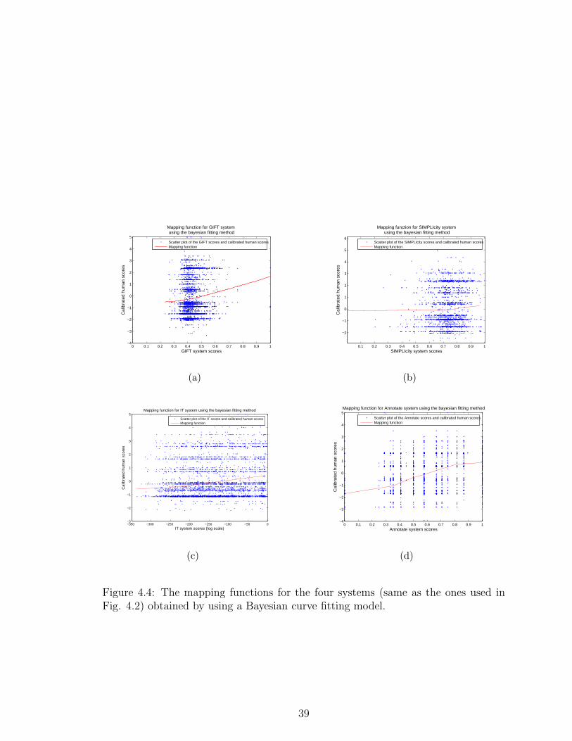
Figure 4.4 illustrates the mapping functions for GIFT, SIMPLIcity, ROMM-

CALIB and Keyword systems obtained by using the constrained Bayesian scheme.

Implementation :

The model we have used is from the biostatistics [49] literature. This model fits

cubic curves between the random points. This information is encoded in the model

parameters M. A more detailed treatment to this subject is given in [49],[50].


CALIB and Keywords obtained by using the constrained Bayesian inference method.

To the reader who is interested in eyeballing performance based on the mapping

functions we encourage them to read the next section.

4.4 Mapping function analysis

The data which is the scatter plot of computer scores and human evaluation scores

is very noisy (Fig. 4.5). If image retrieval systems did better then some of the noise

would have been removed, maybe helping us in eyeballing the performance based on

scatter plots. Explained in the subsequent paragraph is some exploratory work on

eyeballing performance.

For an image retrieval system to do well, the mapped scores should correspond

well to human scores. If the system is perfect the mapped score and human score

correlate to 1 (a straight line). By plotting the mapped score vs human score to we

38

0 0.1 0.2 0.3 0.4 0.5 0.6 0.7 0.8 0.9 1−4

−3

−2

−1

0

1

2

3

4

5

GIFT system scores

Cal

ibra

ted

hum

an s

core

s

Mapping function for GIFT system using the bayesian fitting method


(a)

0.1 0.2 0.3 0.4 0.5 0.6 0.7 0.8 0.9 1

−2

−1

0

1

2

3

4

5

6

SIMPLIcity system scores

Cal

ibra

ted

hum

an s

core

s

Mapping function for SIMPLIcity system using the bayesian fitting method


(b)

−350 −300 −250 −200 −150 −100 −50 0−3

−2

−1

0

1

2

3

4

5

IT system scores (log scale)

Cal

ibra

ted

hum

an s

core

s

Mapping function for IT system using the bayesian fitting method

Scatter plot of the IT scores and calibrated human scoresMapping function

(c)

0 0.1 0.2 0.3 0.4 0.5 0.6 0.7 0.8 0.9 1−4

−3

−2

−1

0

1

2

3

4

5


Cal

ibra

ted

hum

an s

core

s

Mapping function for Annotate system using the bayesian fitting method


(d)

Figure 4.4: The mapping functions for the four systems (same as the ones used inFig. 4.2) obtained by using a Bayesian curve fitting model.

39

Figure 4.5: Scatter plot of the computer score vs. human scores for annotate system.

would like to eyeball performance. Unfortunately, there is a lot of noise (Fig. 4.6),

meaning a highly mapped score has been marked low by the humans. So we smoothed

the scatter plot by a adaptive-binning procedure explained in the follwoing paragraph.

4.4.1 Adaptive-binning

We selected bins on the mapped computer score axes such that all the bins had

roughly the same number of data points. We averaged the human score values in

each bin and plotted the averaged human score vs. mapped computer scores graph.

The averaged human score is for a range of mapped computer scores (bin) so the

center of the bin was chosen as the x-axis representative for the corresponding y-axis

representative of the averaged human score.

We did the same thing with Keyword system scores. We can clearly see the

40

Figure 4.6: The mapped computer scores vs. human scores for GIFT.

difference in performance, with Keyword doing much better (Fig. 4.7).

(a) (b)

Figure 4.7: (a)The adaptively binned and smoothed plot for mapped computer scoresvs. human scores for GIFT and (b) the same for the Keyword system.

41

Chapter 5

Experiments

First, we introduce the performance measures which we employ to compare image

retrieval systems. Next, we study the effect of linear transformations on the variance

across evaluators. Then we compare the four image retrieval systems introduced in

chapter 3. We also compare three low-level feature-extraction algorithms used by the

Gnu-image finding tool (GIFT). Finally, we study the effect of 50% of the data being

evaluated by one person.

5.1 Performance indices

We provide results for several ways to measure the degree to which mapped retrieval

scores agreed with human evaluation scores. Here is the list of such measures:

1. Correlation: We compute the standard correlation between mapped retrieval

results and human evaluations.

2. Precision and recall: We use the human evaluations to define relevant images

42

by setting a threshold (> 3) on the human responses to the query. Hence

the relevance information about a result image is obtained from our ground

truth data. Our measures here follow those of Salton [54], Muller [32] and Van

Rijsbergen [55]. The definition of precision and recall in [54] is adopted in our

studies, which are defined as:

Precision =Number of relevant documents retrieved

Total number of documents retrieved(5.1)

Recall =Number of relevant documents retrieved

Total number of relevant documents in database(5.2)

3. Normalized rank : We report the normalized rank [32] as defined by:

R =1

NNR

NR∑

i=1

(Ri) −NR(NR + 1)

2(5.3)

where N is the collection size, and NR, the number of relevant images, and Ri

is the rank at which the ith relevant image was retrieved. This measure ranges

from 0 to 1, with smaller scores indicating better performance.

5.2 Variance across evaluators

A linear transformation as discussed in §2.4 has been employed to somewhat com-

pensate for the variance among evaluators. The need to compensate for the variance

arises from the diversity and number of participants. To convert the raw user data

into a more useful format we map the mean and variance of the individual participants

to a global mean and variance obtained from the common set.

This achieves the task of penalizing those participants who were lenient and also

43

those that were frugal in their evaluations. Hence this linear transformation maps

the scores of differing evaluators onto a common domain. We validate our belief that

such a grounding, even though simplistic, significantly reduces the variance.

Query by Query by textimage

Interface 1-5 Binary 1-9Number of 24 6 5participantsAverage variance withstandardized scores 1.38 0.19 2.88Average variance withperson dependent adjustment 0.15 0.036 0.937

Table 5.1: Effect of calibration on human scores. The table shows the average stan-dard deviation for standardized scores tabulated for the three sub-experiments beforeand after calibration. Calibration significantly reduces the variance.

Table 5.1 shows the standard error of the results for the common set for each

of paradigms using standardized scores to account for the different ranges and the

analogous values after the removal of bias as described in §2.6. The results show that

variance due to users can be reduced substantively.

Another point of interest is that after having reduced variance through calibra-

tion, there is evidence of still more variance in the human responses on the same

set of images. It is generally observed that as the query-result pairs become more

abstract, the variance increases (Fig. 5.1).

5.3 Comparison of evaluation interfaces

In the query-by-text evaluation, participants that used both the binary and 1-9 inter-

faces reported that the 1-9 interface slowed down their evaluation noticeably. They

felt the range of choices among 1-9 was taxing. Also query-by-text was reported as

44

Figure 5.1: The variance and mean human scores for image pairs in the on-lineevaluation. Shown in the figure are responses from 7 subjects. Many such responsesfrom our pool of participants suggests that as query and result pairs become moreabstract, the greater is the variance.

being more taxing when compared to the query-by-image evaluation. The confusion

was aggravated because the query-by-text method used both one word and two-word

annotations and users expressed confusion over the relevance of either of the words

or both of them.

Since the common set for binary and the 1-9 interface common were the same,

we looked at the relationship between them. Figure 5.2 illustrates the fact that 1-9

results correspond to the binary choices essentially as one would expect. The data

could be used to calibrate between the two interfaces if required.

We also used the 1-5 interface for query-by-image. We noticed that the raw

45

correlation between the measures after calibration suggested that the measures are

in agreement, and we suggest that choosing among them could be based on other

factors. For straightforward benchmarking of retrieval systems we recommend the

data we collected using 1-5 interface as there is more of it.

1 2 3 4 5 6 7 8 90

0.1

0.2

0.3

0.4

0.5

0.6

0.7

0.8

0.9

1

Scoring scheme 2 ( 1−9)

Fra

ctio

ns o

f sco

ring

Sch

eme

1 th

at c

orre

spon

d to

sco

ring

sche

me

2

Fractions of scoring scheme 1 (binary) that correspond to scoring scheme 2 (1−9)

data 2

data 1

Figure 5.2: The fraction of scores from the 1-9 evaluation interface that matchesthe binary evaluations. The data collected by using Scheme 2 is labeled data 2 andsimilarly the data collected using Scheme 1 is labeled data 1.There appears to be agood correlation between the two scoring measures.

5.4 Updating evaluation pair choice based on esti-

mated mapping functions

As discussed earlier in §2.2, the composition of the ground truth data set is critical

for evaluation. Choosing a data set randomly will generate a set with many negative

human responses. In §2.2, we reasoned out the necessity for using a shaping function

46

auxiliary to a bunch of image retrieval systems to select the image pairs for evaluation.

But since the shaping function is only making the data more serviceable we propose

an iterative process that will help us in building a ground truth data set that has a

roughly uniform distribution over human responses. As described in §2.1, once we

have a reasonable amount of evaluation data, we can use the retrieval system specific

mapping functions (§4) to further improve the selection of query/retrieval pairs for

subsequent data collection. A simple measure of uniformity for a human responses

varying over 5 scales is:

error estimate =1

5

5∑

i=1

|p(i) − 0.20| (5.4)

where p(i) is the fraction of responses for category i. Since we use a scale of 1-5 in

collecting the human evaluations, an ideal data set will have equal number of image

pairs marked as either a 1, 2, 3, 4 or 5. Hence the density of an ideal set is uniform

at 0.20.

Tabulated (in Table 5.2) are the error estimates for the data shaped by an arbi-

trary 1/5th power (old data set) and by a new shaping function as dictated by the

mapping function (new data set). The smaller the value of the error estimate the

closer it is to the uniformity over human responses. We observe that there is some

improvement in the distribution of human responses. We posit that iterating the

data set a few more times will show further improvement.

5.5 Comparison of image-retrieval systems

To compare image retrieval algorithms we first find a good mapping of the scores

of that algorithm on the evaluation set to the transformed human scores. First,

47

GIFT SIMPLIcity ROMM-CALIB Keywords

initial data 0.132 0.326 0.176 0.035

mapped data 0.092 0.120 0.103 0.026

Table 5.2: Deviation from uniformity of human evaluation results for data obtainedfrom the four retrieval systems GIFT, SIMPLIcity, ROMM-CALIB; and Keywords.The Keyword system provides selection of image pairs which are closer to the unifor-mity idealism than other systems.

all the three methods (§4.1-§4.3) are used to fit data from the four image retrieval

systems separately and the combined data. Then the mapping method (§4.1-§4.3)

that yields the maximum correlation coefficient on the combined data (data from

all four image retrieval systems) is chosen as a candidate mapping function for that

particular image retrieval system. Finally, this correlation coefficient of the mapped

scores to the human scores depicts the performance of that image retrieval system.

We demonstrate our approach by evaluating content-based image retrieval sys-

tems using the query by image paradigm. These are Semantics-sensitive Integrated

Matching for Picture Libraries (Simplicity) [5], Gnu Image Finding Tool (GIFT) [30]

- [31] (standard feature set as well as using color only), the multipart multi-modal

(M3) image retrieval system and its variants discussed in §2.2 and finally the keyword

retrieval system (§2.1). The results are tabulated in Tables 5.3-5.6.

5.5.1 Correlation measures

In Tables 5.3-5.6 the correlation scores between the mapped scores and the human

evaluation scores for GIFT, SIMPLIcity, ROMM-CALIB and Keyword are tabulated

using the three fitting methods.

This correspondence is calculated for data (query-result pairs) from each of the

48

four image retrieval systems. In this way we have estimated the influence of the

choice of the image retrieval system for selecting query-result pairs.

Correlation between human scoresFitting and mapped GIFT scoresmethods on data selected by different systems

GIFT SIMPLIcity ROMM-CALIB Keywords Mean All

Constrainedleast means 0.18 0.10 0.13 0.10 0.13(0.04) 0.10

squares (§4.1)

Constrainedcorrelation 0.13 0.16 0.26 0.23 0.20(0.03) 0.17

maximization(§4.2)

Bayesianfitting (§4.3) 0.13 0.18 0.22 0.21 0.19 0.10

Table 5.3: The correlation between the mapped scores and the human evaluationscores. The tabulated values are the mean correlation measures for GIFT, as com-puted based on the samples provided from each of the four systems, the average ofthose results, and based on all data combined. Highlighted are the best combinedresult and the best mean correlation score.

The correlation table for SIMPLIcity (Table 5.4) shows that its correlation scores

are in general higher than that obtained for GIFT (Table 5.3). Also in both the

tables the correlation scores are higher on data from ROMM-CALIB and Keywords

compared to GIFT and SIMPLIcity.

49

Correlation between human scoresFitting and mapped SIMPLIcity scoresmethods on data selected by different systems



squares (§4.1)


maximization(§4.2)


Table 5.4: The correlation scores for SIMPLIcity on data from the four image retrievalsystems and combined data (as in Fig. 5.3) using the three fitting methods.

Correlation between human scoresFitting and mapped ROMM-CALIB scoresmethods on data selected by different systems



squares (§4.1)


maximization(§4.2)


Table 5.5: The correlation scores for ROMM (similar to 1.3).

50

Correlation between human scoresFitting and mapped Keyword scoresmethods on data selected by different systems



squares (§4.1)

Constrainedcorrelation 0.25 0.32 0.61 0.57 0.44 (0.17) 0.38

maximization(§4.2)

Bayesianfitting (§4.3) 0.53 0.58 0.62 0.56 0.57(0.04) 0.51

Table 5.6: The correlation scores for Keywords. Emphasized in bold are the perfor-mance descriptors for the divided and combined data sets.

5.5.2 Combined correlation results

To summarize the comparison results we tabulate the correlation scores on the com-

bined data set. The combined data set consists of data pairs from all the four image

retrieval systems. We choose the mapping that yields the best correlation results

for a particular system on combined-data. We then compute the correlation of the

mapped scores to the human scores. The results are in Table 5.7.

5.5.3 Estimated precision-recall curves

We believe that correlation measure gives a quantitative picture of the systems. To

infer other characteristics of performance such as precision and recall curves we can

use our ground truth data. Precision and recall are computed based on the usual

definitions [34].

Typically one would plot the average values of precision verses recall over a thresh-

51

Correlation of the calibrated humanto the mapped system scores

ROMM-ALL 0.24ROMM-TEST 0.17RWMM-ALL 0.35

RWMM-TEST 0.23GIFT 0.17

GIFT-color 0.15GIFT-texture 0.07SIMPLIcity 0.19Keywords 0.51

Table 5.7: Grounded comparison of content based retrieval methods. We report thecorrelation of mapped computer scores with human scores. Each method uses itsown, most favorable, monotonic mapping.

old by modulating the number of images returned. We point out to the reader that

the form of our data is different from the form suggested by the formulas, and thus

producing estimated PR curves requires some modification to the formula.

We have a large number of query-result pairs, which, by design, are a non-uniform

sampling of the space of such pairs. However, since we have many such pairs, if we

weigh the terms to correct for the sampling, then we can estimate the values for the

PR curves. To compute the curves we essentially treat the top M CBIR responses

as a single query for which we can compute the three quantities which are: number

of revelant documents, total number of documents and total number of relevant

documents.

We adjust for the sampling by weighting the terms with the reciprocal of the

sampling function 1. The pseudo-code to calculate precision and recall is given below:

1The amount of data from the iterated approach is only a fraction of the initial data, hencethe reader is informed that this assumption of a uniform shaping function for adjusting the

52

Sort by CBIR score over evaluation set.

This gives human score, h, and a rank, R.

total_relevant = 0;

for curr_pair = 1 to max_num_pairs

{

weight = R^5 (for curr_pair)

if(h > 3) (for curr_pair)

{

total_relevant += weight;

}

}

for num_pairs = 1 to max_num_pairs

{

total = 0;

relevant = 0;

for curr_pair = 1:num_pairs

{ weight = R^5 (for curr_pair);

if(h > 3) (for curr_par)

{

relevant += weight;

}

total += weight

}

}

precision = relevant/total;

recall = relevant/total_relevant;

This includes the number of images retrieved, which is now a weighted sum, not

a count. The estimated PR curves are in Fig. 5.3.

5.5.4 Normalized rank (R)

The normalized rank as defined by [32] suggests a quantitative measure on the rank

of the retrieved images. It measures the error in the rank ordering by image retrieval

systems. If the normalized rank is 1, this suggests that the rank ordering is completely

reversed, which implies that all the images marked as “good” by human evaluations

terms is a fair approximation.

53

0 0.1 0.2 0.3 0.4 0.5 0.6 0.7 0.8 0.9 10

0.1

0.2

0.3

0.4

0.5

0.6

0.7

0.8

0.9

1Estimated Precision−Recall curves

Recall

Pre

cisi

onGIFTSIMPLIictyROMM−TESTROMM−ALLRWMM−TESTRWMM−ALLKeywords

Figure 5.3: Precision recall curves for a number of image retrieval methods. A relevantretrieved image corresponds to an adjusted human evaluation score greater than 3.Because the evaluation set is obtained via shaping functions, we have to estimate thePR curves by reversing the shaping constant in rank. See text for details.

are given a lower computer match score and vice-versa. Hence, the smaller the

normalized rank greater the concurrence with the human score and hence better the

performance. Since the query-result pairs are obtained by sampling, we modify Eq.

5.3 to compensate for the sampling.

In the weighting scheme, we compensate for the effects of sampling by raising the

rank to the reciprocal of the shaping constant, this transforms the data into a series

of power 5. Hence we subtract the sum of the relevant ranks by the sum of the power

5 series which is (2NR6+6NR

5+5NR4−NR

2)12

. To normalize the rank, the denominator is

choosen so as to scale it by imposing the constraint that the worst performance is 1

54

when the rank ordering is reversed. Following the worst-case scenario the normalizing

factor turns out to be 112

[(2NR6+6NR

5+5NR4−NR

2))−(2(N − NR)6+6(N − NR)5+

5(N − NR)4 − (N − NR)2))]

Hence the modified equation is:

R =1

D

NR∑

i=1

(Ri5) −

(2NR6 + 6NR

5 + 5NR4 − NR

2)

12(5.5)

where D is the normalizing factor derived above.

Tabulated (in Table 5.8) are the normalized ranks for the image retrieval systems.

We compare it with when the ranks are assigned randomly and the results suggest

that most of these systems do better than just guessing.

R R on random assignmentROMM-ALL 0.18 0.52

ROMM-TEST 0.20 0.51RWMM-ALL 0.14 0.52

RWMM-TEST 0.15 0.52GIFT 0.28 0.53

SIMPLIcity 0.27 0.51Keywords 0.06 0.51

Table 5.8: Normalized ranks for each of the image retrieval systems without/withrandom selection. The results suggest that each system performs much better whenthe ranks are not assigned randomly.

5.6 Effect of half of the ground truth developed by

one person

This experiment involved segregating the data obtained by the author and others and

computing the correlation scores for the image retrieval systems. If the correlation

55

values lie in the same ballpark as that obtained by running the tests on combined

data, then we can negate the criticism of being biased in our ground truth. In

either case we need to collect more data from others. Tabulated in Table 5.9 are the

correlation scores along with the standard error for the retrieval systems discussed

in §5.5 on data obtained from one person, the rest and the combined data. The

correlation scores on data from three sources are within the standard errors of each

other suggesting that there does not appear to be a bias in the ground truth data.

Systems author others combinedROMM-ALL 0.21 (0.03) 0.19 (0.04) 0.24 (0.01)

ROMM-TEST 0.20 (0.03) 0.19 (0.02) 0.17 (0.02)RWMM-ALL 0.24 (0.03) 0.25 (0.03) 0.35 (0.03)

RWMM-TEST 0.23 (0.04) 0.22(0.03) 0.23 (0.03)GIFT 0.17 (0.02) 0.20 (0.03) 0.17 (0.01)

SIMPLICITY 0.16 (0.03) 0.21 (0.02) 0.19 (0.01)KEYWORDS 0.57 (0.04) 0.50 (0.05) 0.51 (0.02)

Table 5.9: Correlation scores of image retrieval systems on data obtained from theevaluations of the author, others and the combined data.

5.7 Evaluating text queries

The query-by-text paradigm was also calibrated using data collected from the on-

line text-query based interface §2. The score was based on a simple match between

the text associated with the query and result images. If we denote the set of words

associated with the query image as WQ, and the set of words associated with the

retrieved image as WR, and the number of elements in a set W by |W |, then the

keyword score is given by:

score =|WQ ∩ WR|

min(|WQ|, |WR|)(5.6)

56

After mapping the scores in the similar manner as discussed in §4, we obtain

the correlation values for the correspondence between the mapped scores and the

calibrated human scores. The query by text using keywords does better than most of

the image retrieval systems based on image features. Also Corel images already have

tagged keywords. Hence, we propose using keywords match as a proxy to evaluate

image retrieval systems.

The correlation between the proxy score and the human score developed in §4 is

0.58. This suggests that while such scores are a valid indicator of retrieval perfor-

mance, it fails to capture a significant part of what the human evaluators expect from

a retrieval system. It is possible that a better text-based measure could be found,

and this is the subject of ongoing work by the Benchathlon project.

5.8 Comparison of low-level features in GIFT

We calibrate feature extraction algorithms used by GIFT. We tested the performance

of low-level features by operating GIFT in three modes:

1. Gift (color + texture): In this mode, GIFT has access to both local and global

color and spatial frequency features.

2. Gift (color): Gift uses only the local and global color features for indexing and

retrieval.

3. Gift (texture): Gift uses only the local and global spatial frequency features for

indexing and retrieval.

57

Evaluated feature Correlation score (mean)Color only 0.18

Texture only 0.07Texture and Color 0.19

Table 5.10: Correlation scores for the low -level features used by GIFT, in standalonemode. We observe that color alone does almost as well as the combination of colorand texture.

5.9 Summary

In this chapter we present the comparison of image retrieval systems and algorithms.

Summarizing the chapter:

1. We firstly presented a validation of our theory that linear transformation is a

useful way to reduce the variance between evaluators. A simplistic approach

like a linear-transformation is shown to considerably reduce the variance.

2. We present the correlation scores for systems based on three mapping methods

and data from four retrieval systems. Even though the rank ordering of systems

based on performance varied with data and mapping methods, we establish

in the combined results that the favorable score on each system suggests a

performance ordering of the form: Keywords > RWMM-ALL > RWMM-TEST

> ROMM-ALL > SIMPLIcity = ROMM-TEST > GIFT.

3. We modify the general definition of precision-recall to accommodate for the

sampling we have used and confirm the rank ordering of systems based on

performance as suggested by the correlation scores. This validates our ground

truth data in a certain sense, as two disparate measures concur.

4. Finally we introduce the concept of normalized rank and discuss ways to com-

58

pute it based on our sampling. These results indicate that the rank ordering

statistics of systems and system performance ranking follow the same pattern

as the PR-curves.

59

Chapter 6

Conclusions

We have developed a system for making user-grounded comparisons of image re-

trieval systems. Importantly, the data and software applies to the evaluation of any

image retrieval system because we only consider the input-output relation for each

of the systems. We have made the data and calibration software available on-line

[http://kobus.ca/research/data [19]].

In Chapter 1. we introduced the readers to the concept of evaluation of image

retrieval systems and explained why this is an arduous task. In Chapter 2. we

explained our approach of collecting user-grounded data and proposed to develop

ground truth data. We emphasized the need for an approximate uniformity in the

selection of image pairs over human responses. In §2.2 we described a shaping function

that when used auxiliary with image retrieval systems produced a more serviceable

ground truth data. In Chapter 3. we introduced the image retrieval systems that

were used to select the image pairs and also served as a test case for comparing

image retrieval systems with our methodology. In Chapter 4. we elucidated the need

60

for mapping disparate computer scores to a common domain of human scores in a

constrained fashion, to obtain the mapped scores. We have established the correlation

between the human scores and the mapped scores as a performance measure.

In this thesis we have developed a process to measure the performance of image

retrieval systems. This process establishes a mapping from the computer scores to the

human evaluation scores and performance is given by the degree of correspondance

between the mapped scores and human scores. One of the significant contributions

of this thesis is the ground-truth data collected for about 16,000 image pairs. We

have been cautious in the selection of query-result pairs. We have used four image

retrieval systems influenced by a shaping function so as to get a roughly uniform

distribution on human responses. We observed that data being selected by different

image retrieval systems made little difference to the performance ordering of the

systems. We have also taken caution in reducing the variance among evaluators.

The results of the comparisons showed that keyword (text) retrieval outperformed

the image-based methods. This reflects the fact that keywords capture the semantics

of images better than the existing image-based methods. This is also corroborated

by user studies which suggest that semantics played a dominant role in what users

consider a relevant match, and that the computer algorithms failed to completely

capture the image semantics from image features. These results hint at the possibil-

ity of using annotation-oriented evaluation as a proxy for user-directed evaluation.

However, the results suggested that the scope of such a proxy is limited since the

keyword results were far from perfect. A significant portion of what our participants

expressed through their choices is not captured, and thus not measurable using the

keyword proxy. Since the annotation system outperformed image-based methods, we

posit that using a combination of keywords and image features may lead to better

61

performance. We verified this hypothesis, as RWMM performance is superior to that

of ROMM. We see the image features method (ROMM-ALL) to be an alternative

method to SIMPLIcity in that it reports a match over several image regions. How-

ever, while ROMM-ALL models the statistics of the data, SIMPLIcity computes the

matches on the fly. We found that ROMM-ALL performs a bit better than SIMPLIc-

ity, but further investigation is called for here. When forced to model on the test set

(images not in the training set), eg. ROMM-TEST, the performance of the model

is worse than SIMPLIcity, and same as GIFT. The results from the RWMM-TEST

indicate that the word and feature together are closely related and that this is a good

model for generalization as the correlation scores for RWMM-TEST are comparable

to that of RWMM-ALL.

We demonstrated the consistency of the results by showing that all the measures,

(correlation scores, estimated precision-recall plots and the normalized rank) concur

in the performance ordering of the image retrieval systems. Herein lies the proof

of the concept that human evaluations, once grounded can be used as ground truth

data for evaluating image retrieval systems and algorithms. The applications of this

benchmarking process are plentiful. One such application is evaluating computer

vision algorithms that could be plugged into image retrieval systems. Also improv-

ing image retrieval systems based on performance on the ground-truth data is an

interesting application. Employing our process to evaluating keyword retrieval could

prove to be insightful. For example, in the Corel image data, there are many images

that have the keyword sky, but only a few of them would be of interest to a human

user searching for a sky photograph. The information being sought by the user is

linked to the semantics of the image. The semantics of the image could be encoded

in terms of annotation, image features or a combination of both. Thus we hope that

62

by evaluating keyword annotation, our approach and our data will lead to a better

understanding of the limitations of keyword search, and suggest ways on how it can

be improved.

The next step is to integrate our approach with a new data set which is explicitly

designed for image understanding and retrieval research and free of copyright issues.

We will also study in more detail ways to reduce participant variance. Also in the

pipeline are iterating the data selection process a few more times to get it closer to

our uniformity ideal. We also expect to expand the scale of data collection to include

more participants, more data, and more data selection methods.

In conclusion, we have a proof of concept on a method for evaluating image

retrieval systems and we wish to help others evaluate and improve their retrieval

systems.

63

Appendix A

Data and Code description

A.1 Data

This section contains description of the data and code used in the CVPR paper “Eval-

uating Image Retrieval” [67]. The data was collected using an on-line evaluation tool.

The on-line interface was developed and is being maintained by the author. The data

is due to the collective effort of 32 students and we are thankful for their help. This

ground truth data is available for download at (http : //kobus.ca/data/research).

A.1.1 Data Description

The data consists of human evaluation scores for pairs of query-result images. The

pre-processing step involved an iterative selection of the query-result pairs such that

they span the broad spectrum of choices. We cannot choose query/result images at

random as most of them will be judged as a poor match, hence resulting in poor data.

The main stratergy is to use existing image retrieval systems to select serviceable

64

image pairs. Unfortunately, current image retrieval systems do not work very well,

hence we propose using a non-linear function auxiliary to the retrieval system to

obtain a roughly uniform distribution over the choices. We also concenterated our

efforts on collecting more data as this will allow us to be approximate in the uniformity

but still have enough examples over the human responses. The data consisted of

query-result pairs from four content-based image retrieval systems. This setup is

observed so as to be cautious against introducing abnormalities in the data because

of irregularities in a particular image retrieval system.

The experimental routine was as follows: First, the query image and result im-

ages from the four CBIR systems were displayed in random order. Then the user

rated each match on a scale of 1 to 5 with 1 being a poor match and 5 a good

match. We ensured that the first 100 queries are common to all users and computed

a linear transformation so as to reduce the variance among evaluators. The rest of

the images evaluated by the users, are unique. Having reduced the variance using

the suggested transformation, we now have in place a ground-truth data. To obtain

a common domain of absolute scores, we mapped the computer scores to the ad-

justed human scores by three mapping methods. The mapping method that yielded

the best correlation was retained. The agreement between the mapped scores and

the adjusted human scores gave a indication of performance. Also, the data gives

us options to measure precision-recall and normalized-rank. We present the image

retrieval community with a data set of image pairs marked with a relevance score.

The other data available for download is the annotation ground-truth system.

This data is obtained from the annotation engine of Kobus’ system [37]. The data

consists of an annotation score for the same query-image pairs. We propose that this

data set could be used as a proxy to measure performance.

65

In order to allow researches use our data we have made the groundtruth data

freely downloadable. For choice of performances indices, you could refer [67] or

you could come up with your own. The database we use in our research was pro-

vided by Corel. This database has copyright restrictions and may not be freely

distributed. But for those researches who have access to the Corel, our ground-

truth data should simplify things because we use Corel’s indexing scheme. We hope

to develop a copyright free database in the future. For any information regarding

benchmarking contact: Nikhil Shirahatti ([email protected]) OR Kobus Barnard

([email protected])

A.2 Code

The benchmarking suite Retrieval Analyzer includes a collection of three map-

ping methods described below. The inputs to Retrieval Analyzer are a vector of

computer scores (your image retrieval scores for the image pairs we have provided

in our ground truth data) and corresponding human scores (our ground truth data).

The outputs consist of a correlation score, an estimated precision-recall curve and

an estimated normalized rank. We provide an option for choosing from any of the

three mapping methods, but we recommend using the default option which chooses

the mapping method that maximizes the correlation score.

A.2.1 Support

This suite has been tested on Linux (Redhat and Fedora distributions). We have

not tested it on any other unix/linux platforms. Most of the suite of tools does not

work on Microsoft Windows. However, if you are succesfull in porting this program

to either Windows or a different linux/unix distribution, then we encourage you to

66

share it with others. Send the author an email and we will be happy to setup a link

to a ported version.

A.2.2 Terms of Use

The use of this software and data is restricted to educational and research purposes.

Modifying the code is encouraged, as long as appropriate credit is provided, and

authorship is not misrepresented. If you would like to make commercial use of any

of the code being distributed, then please contact the author ([email protected]).

If you make use of this software for your research, we would appreciate it if you

cite or acknowlege the web site and/or the “Evaluating Image Retrieval”.

A.2.3 Credits

Thanks to Prof. Kobus Barnard who, as my advisor helped me understand the

problem and guided me in my efforts to solve this benchmarking bugaboo. It is the

team effort of both of us that we have working model of an image retrieval evaluation

system. Kudos to all the participants who have helped me collect an appreciable

amount of data. Also, many thanks to Prof. Nicholas Heard for providing with the

source code for a bayesian approach to curve fitting. My regards to Mathworks for

providing the optimization toolkit.

A.2.4 Installation

Once you have downloaded, unzipped, and untarred, the benchmarking suite.tar.gz

you will have three directories.

1. Code: It contains a number of matlab files listed below, and a script file. The

67

files are:

• code/clmsSys.m – matlab code for performing constrained least means

squared fitting

• code/ccmSys.m – matlab code for performing constrained correlation max-

imization fitting

• code/getRand.m – random sampling of a vector of values

• code/myfunc.m – the function minimized in ccmSys.m

2. Data: This consists of a test file which is a part of the results published in the

paper “Evaluating Image Retrieval”. This data consists of computer scores for

images selected using the GNU image finding tool. This data forms a part of

our ground truth data.

3. Result: On running the scripts the results are put into a text file “results.txt”

in this directory. This text file contains the correlation scores using the two

mapping methods.

68

Bibliography

[1] M. Flickner, H. Sawhney, W. Niblack, J. Ashley, Q. Huang, B. Dom, M. Gorkani,

J. Hafner, D. Lee, D. Petkovic, D. Steele, and P. Yanker, Query by image and

video content: The QBIC system , IEEE Computer, vol. 28, pp. 22-32, 1995

[2] S. Sclaroff, L. Taycher, and M. La Cascia, ImageRover: A content-based image

browser for the World Wide Web, Proc. IEEE Workshop on content-based access

of image and video libraries, 1997

[3] M. La Cascia, S. Sethi, and S. Sclaroff, Combining Textual and Visual Cues for

Content-based Image Retrieval on the World Wide Web, Proc. IEEE Workshop

on Content-Based Access of Image and Video Libraries, 1998.

[4] C. Carson, S. Belongie, H. Greenspan, and J. Malik, Blobworld: Color and

Texture-Based Image Segmentation Using EM and Its Application to Image

Querying and Classification, IEEE Trans. Patt. Anal. Mach.Intell., vol. 24, pp.

1026-1038, 2002

[5] J. Z. Wang, J. Li, and G. Wiederhold, SIMPLIcity: Semantics-Sensitive Inte-

grated Matching for Picture Libraries, IEEE Trans. Patt. Anal. Mach. Intell., vol.

23, pp. 947-963, 2001.

[6] J. Cox, M. L. Miller, T. P. Minka, T. V. Papathomas, and P. N. Yianilos, The

Bayesian Image Retrieval System, PicHunter: Theory, Implementation and Psy-

chophysical Experiments, IEEE Transactions on Image Processing, vol. 9, pp.

20-35, 2000

69

[7] W. M. Smeulders, M. Worring, S. Santini, A. Gupta, and R. Jain, Content-Based

Image Retrieval at the End of the Early Years, IEEE Transactions on Pattern

Matching and Machine Intelligence,vol. 22, pp. 1349-1379, 2000

[8] W. Y. Ma and B. S. Manjunath, NeTra: A toolbox for navigating large image

databases, Multimedia Systems, vol. 7, pp. 84-198, 1999

[9] A. Pentland, R. Picard, and S. Sclaroff, Photobook: Tools for Content-Based

Manipulation of Image Databases, SPIE Storage and Retrieval of Image and Video

Databases II, Feb 1994.

[10] P. G. B. Enser, Progress in documentation pictorial information retrieval, Jour-

nal of Documentation, vol. 51, pp. 126-170, 1995.

[11] P. G. B. Enser, Query analysis in a visual information retrieval context, Journal

of Document and Text Management, vol. 1, pp. 25-39, 1993.

[12] L. H. Armitage and P. G. B. Enser, Analysis of user need in image archives,

Journal of Information Science, vol. 23, pp. 287-299, 1997.

[13] M. Markkula and E. Sormunen, End-user searching challenges indexing practices

in the digital newspaper photo archive, Information retrieval, vol. 1, pp. 259-285,

2000.

[14] D. A. Forsyth, Benchmarks for storage and retrieval in multimedia databases,

Proc. Storage and Retrieval for Media Databases III, San Jose, 2002.

[15] S. Ravela , R. Manmatha, Retrieving Images by Similarity of Visual Appearance,

Proceedings of the 1997 Workshop on Content-Based Access of Image and Video

Libraries (CBAIVL ’97), 67-74, 1997

70

[16] Joseph L.Lundy and Andrew Zisserman, editors. Geometric invariance in Com-

puter Vision. The MIT Press, 1992.

[17] J. R. Smith, Image retrieval evaluation, Proc. IEEE Workshop on content-based

access of image and video libraries (CBVAILVL), Santa Barbara, CA, 1998

[18] J. Vogel and B. Schiele, On Performance Characterization and Optimization for

Image Retrieval, Proc. 7th European Conference on Computer Vision, Copen-

hagen, Denmark, pp. 49-63, 2002.

[19] J. Z. Wang and J. Li, Learning-based linguistic indexing of pictures with 2-D

MHMMs, Proc. ACM Multimedia, Juan Les Pins, France, pp. 436-445, 2002

[20] N. J. Gunther and G. B. Beratta, Benchmark for image retrieval using distributed

systems over the Internet: BIRDS-I, Proc. Internet Imaging III, San Jose, pp.

252-267, 2001

[21] T. Pfund and S. Marchand-Maillet, Dynamic multimedia Keywords tool, Proc.

Internet Imaging III, San Jose, pp. 206-224, 2002.

[22] The Benchathlon Network, www.benchathlon.net

[23] C. Jorgensen and P. Jorgensen, Testing a vocabulary for image indexing and

ground truth, Proc. Internet Imaging III, San Jose, pp. 207-215, 2002

[24] Liu Wenyin, Zhong Su, Stan Li, Yan-Feng Sun, Hongjiang Zhang, A

Performance Evaluation Protocol for Content-Based Image Retrieval Algo-

rithms/Systems, Proc. IEEE CVPR Workshop on Empirical Evaluation in Com-

puter Vision, Kauai, USA, December, 2001

[25] Corel database http://www.corel.com

71

[26] Susanne Ornager, The newspaper image database: empirical supported analysis

of users’ typology and word association clusters, Annual ACM Conference on

Research and Development in Information Retrieval, Proceedings of the 18th

annual international ACM SIGIR conference on Research and development in

information retrieval, 212-218, 1995

[27] Keistler, Lucinda H, User types and queries: Impact on image access system.

In: Challenges in Indexing Electronic Text and Images, Ed. by Raya Fidel et al.

ASIS Monograph Series. Learned Information Inc., Medford, NJ, pp. 7-22, 1994

[28] Markey, K, Access to iconographical research collections. Library Trends , 37(2),

154-174, 1984

[29] Hastings, S.K, Query categories in a study of intellectual access to digitized art

images, Proceedings of the 58th Annual Meeting of the American Society for

Information Science, October 9-12, 1995, Chicago, IL (pp. 3-8). Medford, NJ:

ASIS

[30] Henning Muller,Stephane Marchand-Maillet and Thierry Pun, The Truth about

Corel - Evaluation in Image Retrieval, Proceedings of the International Confer-

ence on Image and Video Retrieval table of contents Pages: 38 - 49, 2002.

[31] H. Muller, W. Muller, D. M. Squire, and S. Marchand-Maillet, Performance

Evaluation in Content-based Image Retrieval: Overview and Proposals, Pattern

Recognition Letters, vol. 22, pp. 593-601, 2001

[32] D. M. Squire, W. Muller, H. Muller, and J. Raki, Content-based query of image

databases, inspirations from text retrieval: inverted files, frequency-based weights

72

and relevance feedback, Computer Vision Group, Computing Center, University

of Geneva 98.04, 1998

[33] Available from www.gnu.org/software.gift

[34] G. Salton, The State of retrieval system evaluation, Information Processing and

Management, vol. 28, pp. 441-450, 1992

[35] P. Duygulu, K. Barnard, J. F. G. D. Freitas, and D. A. Forsyth, Object recogni-

tion as machine translation: Learning a lexicon for a fixed image vocabulary, The

Seventh European Conference on Computer Vision, IV:97-112 , 2002

[36] K. Barnard, P. Duygulu, N. D. Freitas, D. Forsyth, D. Blei, and M. I. Jordan,

Matching Words and Pictures, Journal of Machine Learning Research (in press)

[37] Kobus Barnard, Pinar Duygulu, and David Forsyth, Exploiting Text and Image

Feature Co-occurrence Statistics in Large Datasets, to appear as a chapter in

Trends and Advances in Content-Based Image and Video Retrieval (tentative

title)

[38] Kobus Barnard, Pinar Duygulu, and David Forsyth, Recognition as Translating

Images into Text, Internet Imaging IX, Electronic Imaging 2003 (Invited paper)

[39] T. Hofmann, Learning and representing topic. A hierarchical mixture model for

word occurrence in document databases, Workshop on learning from text and the

web, 1998

[40] Jianbo Shi, Jitendra Malik, Normalized Cuts and Image Segmentation, IEEE

Transactions on Pattern Analysis and Machine Intelligence, 888-905, 2000

73

[41] J.A. Hartigan and M.A. Wong, Algorithm AS136: A k-means Clustering Algo-

rithm, Applied Statistics, vol. 28, pp. 100-108, 1979

[42] I. Daubechies, Ten Lectures on Wavelets. Philadelphia: SIAM, 1992

[43] Michael J. Swain, Dana H. Ballard, Color indexing, International Journal of

Computer Vision, 11 - 32, 1991

[44] R. Gonzalez and R. Woods, Digital Image Processing, Addison Wesley, 14 - 428,

1992

[45] B. Efron, and R.J Tibshirani, An introduction to the bootstrap, New York, Chap-

man and Hall, 1993

[46] Coleman, T.F. and Y. Li, A Reflective Newton Method for Minimizing a

Quadratic Function Subject to Bounds on some of the Variables, SIAM Journal

on Optimization, Vol. 6, Number 4, pp. 1040-1058, 1996.

[47] Coleman, T.F. and Y. Li, On the Convergence of Reflective Newton Methods for

Large-Scale Nonlinear Minimization Subject to Bounds, Mathematical Program-

ming, Vol. 67, Number 2, pp. 189-224, 1994

[48] C.C. Holmes and N.A. Heard, Generalized monotonic regression using random

change points, Statistics in Medicine, 22, 4, 623-638, 2000

[49] N. A. Heard and Adrain Smith, Bayesian piecewise polynomial modeling of ogive

and unimodal curves, Technical report, 2002

[50] N. Metropolis, A.W. Rosenbluth, M.N. Rosenbluth, A.H. Teller, and E. Teller,

Equations of State Calculations by Fast Computing Machines, Journal of Chemical

Physics, 21:1087-1091, 1953

74

[51] W.K. Hastings, Monte Carlo Sampling Methods Using Markov Chains and Their

Applications, Biometrika, 57:97-109, 1970

[52] T. Robertson, F.T. Wright, R.L. Dykstra, Order-Restricted statistical Inference,

Wiley: New York, 1988

[53] M.J. Schell, B. Singh, The reduced monotonic regression method, Journal of the

American Statistical Association, 92(437):128 135, 1997

[54] G. Salton, The State of retrieval system evaluation, Information Processing and

Management, vol. 28, pp. 441-450, 1992

[55] C. J. Van Rijsbergen, Information retrieval, London, Butterworths, 1979

[56] Visual information E6850 course assignment at Columbia University taught by

Prof. Chang, http : //www.ee.columbia.edu/ sfchang/course/vis/

[57] Kobus Barnard, Nikhil V Shirahatti, A method for comparing content based

image retrieval methods, Internet Imaging IX, Electronic Imaging 2003

[58] G. Ciocca, R. Schettini, A relevance feedback mechanism for content-based image

retrieval, Information Processing and Management, Vol. 35, pp. 605-632, 1999.

[59] John A. Black Jr., Gamal Fahmy, Sethuraman Panchanathan A., Method for

Evaluating the Performance of Content-Based Image Retrieval Systems Based

on Subjectively Determined Similarity between Images,Conference on Image and

Video Retrieval, 356-366, 2002.

[60] Minka, T. P., and Picard, R. W, Interactive learning with a society of models’,

Pattern Recognition, 30(4), 565-581, 1997

75

[61] Sanchez, D., Chamorro-Martinez, J., and Vila, M. A, Modeling subjectivity in

visual perception of orientation for image retrieval, Information Processing and

Management, 39(2), 251-266, 2003

[62] Squire, D. M., and Pun, T, Assessing agreement between human and machine

clustering of image databases, Pattern Recognition, 31(12), 1905-1919, 1998

[63] Wu, J. K., and Narasimhalu, A. D, Fuzzy content-based retrieval in image

databases, Information Processing and Management, 34(5), 513-534, 1998

[64] Tsai, C.F., McGarry, K., and Tait, J, Qualitative evaluation of automatic as-

signment of keywords to images, International Journal of Information Processing

and Management, 2005 (In Press).

[65] Zhao R., Grosky W. I., Bridging the semanitic gap in image retrieval, Content-

based retrieval and image database techniques, 14 - 36, 2002

[66] Smeulders A W M, Worring M, Santini S, Gupta A, Jain R., Content-Based

Image Retrieval at the End of the Early Years, IEEE Transactions on Pattern

Analysis and Machine Intelligence, 22: 12, 1349 - 1380, 2000

[67] Nikhil V. Shirahatti and Kobus Barnard,Evaluating Image Retrieval, Conference

on Computer Vision and Pattern Recognition, to appear, 2005.

76

evaluating image retrieval

Documents