On Evaluating Methods for Recovering Image Curve Fragments

Yuliang Guo and Benjamin KimiaBrown University, Division of Engineering

{33yuliangguo@gmail.com, kimia@lems.brown.edu}

Abstract

Curve fragments, as opposed to unorganized edge ele-ments, are of interest and use in a large number of applica-tions such as multiview reconstructions, tracking, motion-based segmentation, and object recognition. A large num-ber of contour grouping algorithms have been developed,but progress in this area has been hampered by the fact thatcurrent evaluation methodologies are mainly edge-based,thus ignoring how edges are grouped into contour segments.We show that edge-based evaluation schemes work poorlyfor the comparison of curve fragment maps, motivating twonovel developments: (i) the collection of new human groundtruth data whose primary representation is contour frag-ments and where the goal of collection is not distinguishedobjects but curves evident in image data, and (ii) a method-ology for comparing two sets of curve fragments whichtakes into account the instabilities inherent in the forma-tion of curve fragments. The approach compares two curvefragment sets by exploring deformation of one onto anotherwhile traversing discontinuous transitions. The geodesicpaths in this space represent the best matching between thetwo sets of contour fragment. This approach is used to com-pare the results of edge linkers on the new contour fragmenthuman ground truth.

1. INTRODUCTIONEdges and contours are subtle concepts. We all see them

in images. They arise from multiple and diverse physi-cal sources, including occluding contours, reflectance dis-continuities, surface discontinuities, texture discontinuities,shade curves, shadows, and highlights. They are also per-ceived when no physical correlate exists, i.e., at illusorycontours. Numerous computer vision algorithms have beendeveloped to capture these image contours, typically as in-put to facilitate object recognition, tracking, 3D reconstruc-tion, and other vision tasks.

These algorithms have had to face the elusive nature ofedge detection and contour extraction [21, 11, 8, 6, 1, 19, 18,25]. An edge is a point of significant local change in inten-

sity, color, texture, etc. . A contour fragment is a groupingof a number of edges as an ordered sequence of points. Akey component of progress in this area has been the devel-opment of Evaluation Strategies and databases [5, 4, 20], inparticular the Berkeley Segmentation Dataset (BSDS) andthe USF datasets [5]. These datasets have generally focusedon evaluating edges. Unfortunately, datasets featuring con-tour fragments are currently lacking. Thus, the current eval-uation of algorithm to recover contours, or a linked set ofedges, has fallen back on evaluating them against humanannotation at the level of edges [8, 26]. This has preventedan evaluation of the quality of the grouping of edges intoan ordered sequence of edges: under evaluation based onedges considers, all grouping of edges are considered a sin-gle equivalence class.

While it is possible to generate contour fragments fromsome of the existing datasets, these contours are boundariesof regions, split into contour fragments based on region-based constraints. In addition, numerous types of contourfragments are excluded in this process. Hand in hand withthe lack of proper data sets for comparing a set of contourfragments, evaluating strategies also have focused on com-paring two unorganized set of edge maps and methods forcomparing two contour fragment sets are currently lacking.

The contribution of this paper is twofold. The firstcontribution is to develop a new type of human annotatedground truth centered on contour fragments, as motivatedby several factors: (i) a shift of focus is needed from edgesto contour fragments; (ii) a shift in perception on what typesof contours need to be represented and extracted: the de-velopment of BSDS was based on the idea that only se-mantically meaningful contours, i.e.those that define objectboundaries and are central to task such as object recogni-tion should be represented in the human annotation and thisis also what is expected of an algorithm for extracting con-tour fragments. However, there are numerous other types ofimage curves which reflect structure in the world and canthus be used in a variety of applications, e.g., reflectancepatterns such as zebra stripes, a fold on a wing of a swan, ahigh light on an apple, a muscular definition on the hind legof a horse, etc. , which can be used in a variety of applica-

1

tion, such as multiview reconstruction based on curves [7],tracking in a video [14], motion segmentation [13, 12]. Inaddition, they can be used in object recognition with addi-tion processing.

The BSDS is not appropriate for the evaluation of sucha diverse set of images curves since its goal is evaluationof semantic curves and restricted to closed curves, and allveridical open curves are noted as false positives. A shiftaway from semantic contours as object silhouettes to a di-verse ragee of images curves which rely 3D structure inthe form of objects requires a shift from closed curve toopen curve fragment and a shift from semantic contoursto perceived contours. We have developed a methodologyfor collecting a human-annotated ground-truth database ofperceived contours using 30 images selected from BSDSimages and three human subjects. This Contour FragmentGround-Truth Dataset (CFGD), which is publicly available,does not invalidate the role of BSDS in evaluating semanticcontours. Rather, CFGD can be used to evaluate contourfragments on the way to constructing semantic contours.

As a second contribution of this paper, we develop amethodology for comparing two sets of contour fragments.A key difficulty in comparing two contour fragments is theinherent instability of the edge linking process.. For ex-ample a long contour might be split in two shorter contourfragments. In contrast to such an instability, which doesnot reflect structural differences between the two group-ing, there are other groupings which are fundamentally dis-tinct. We adopt an“edit distance” approach, e.g.where splitcontours can be merged so that corresponding subsets ofcontour fragments can be revealed, leaving missing/extracorrespondences. We show that using this novel approachto comparing two sets of contour fragments, edge linkingmethods for extracting contour fragments can be evaluatedon the newly developed dataset.

2. BSDS is not optimal for evaluating ContourFragments

One of the most popular segmentation datasets is theBerkeley Segmentation Data Set (BSDS) [20]. The statedgoal of this work is to provide an empirical basis for eval-uation of image segmentation and boundary detection [9].The BSDS300 dataset consists of 1,000 Corel dataset im-ages for which 12,000 hand-labeled segmentations of from30 human subjects have been collected. The BSDS500 isan extension of the BSDS300 where 200 new images areadded, together with human annotations.

This database has been extensively used for the evalu-ation of both segmentation and boundary detection algo-rithms [8, 18, 22, 2, 6], as evidenced by over 1200 citations,Figure 1. Prior to the establishment of the BSDS databases,research articles typically showed a few results, likely to betheir best examples, but typically not clear what the typical

examples look like, nor what the failure modes are. With-out a formal evaluation, such questions could not be an-swered even by highly objective researchers. While someresearchers advocated task-orientated evaluation [4], Mar-tin et al. proposed to use multiple human data to evaluatethe intermediate segmentation results [20]. The dataset thusprovides a valuable evaluation framework.

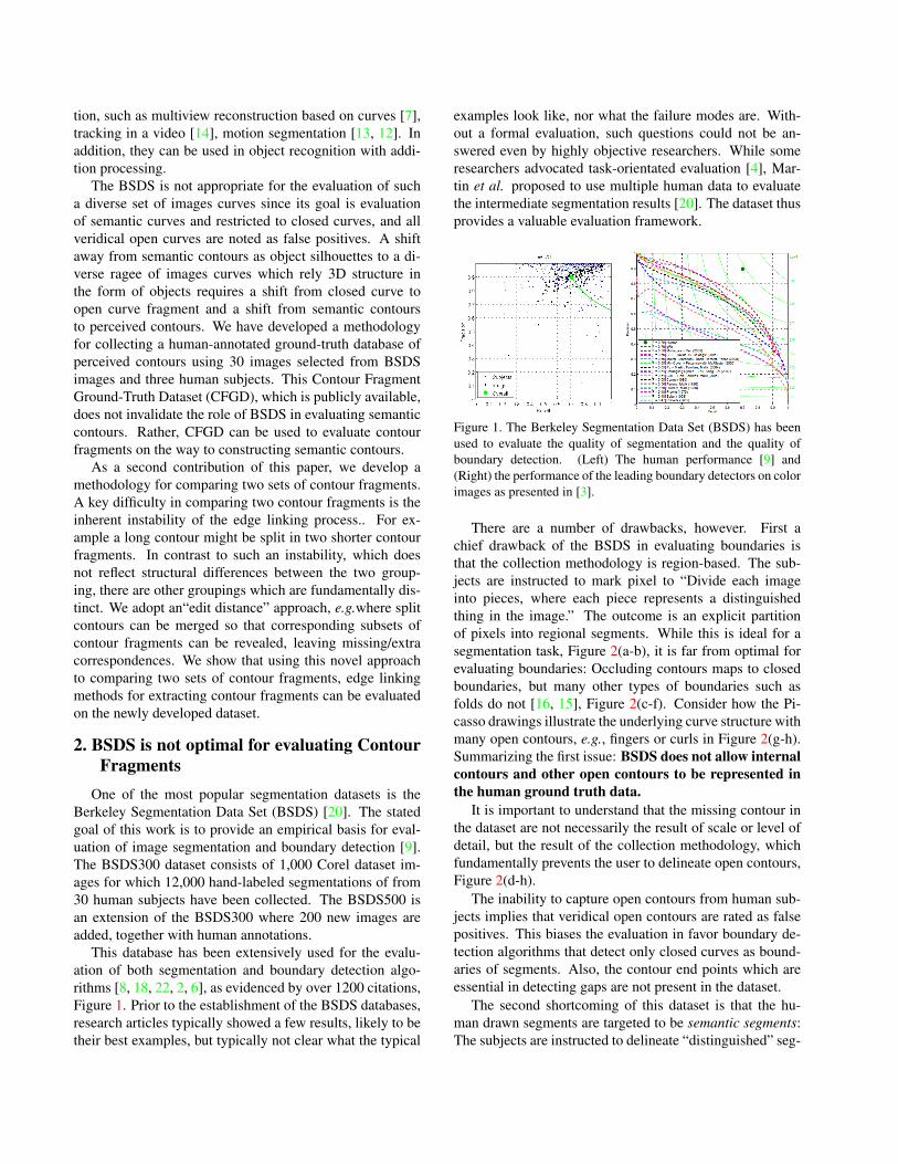
Figure 1. The Berkeley Segmentation Data Set (BSDS) has beenused to evaluate the quality of segmentation and the quality ofboundary detection. (Left) The human performance [9] and(Right) the performance of the leading boundary detectors on colorimages as presented in [3].

There are a number of drawbacks, however. First achief drawback of the BSDS in evaluating boundaries isthat the collection methodology is region-based. The sub-jects are instructed to mark pixel to “Divide each imageinto pieces, where each piece represents a distinguishedthing in the image.” The outcome is an explicit partitionof pixels into regional segments. While this is ideal for asegmentation task, Figure 2(a-b), it is far from optimal forevaluating boundaries: Occluding contours maps to closedboundaries, but many other types of boundaries such asfolds do not [16, 15], Figure 2(c-f). Consider how the Pi-casso drawings illustrate the underlying curve structure withmany open contours, e.g., fingers or curls in Figure 2(g-h).Summarizing the first issue: BSDS does not allow internalcontours and other open contours to be represented inthe human ground truth data.

It is important to understand that the missing contour inthe dataset are not necessarily the result of scale or level ofdetail, but the result of the collection methodology, whichfundamentally prevents the user to delineate open contours,Figure 2(d-h).

The inability to capture open contours from human sub-jects implies that veridical open contours are rated as falsepositives. This biases the evaluation in favor boundary de-tection algorithms that detect only closed curves as bound-aries of segments. Also, the contour end points which areessential in detecting gaps are not present in the dataset.

The second shortcoming of this dataset is that the hu-man drawn segments are targeted to be semantic segments:The subjects are instructed to delineate “distinguished” seg-

(a) (b) (c) (d)

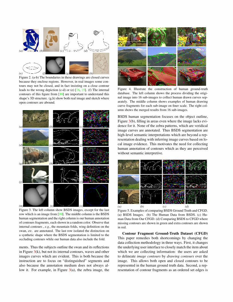
(e) (f) (g) (h)Figure 2. (a-b) The boundaries in these drawings are closed curvesbecause they enclose regions. However, in real images some con-tours may not be closed, and in fact insisting on a close contourleads to the wrong depiction (c-d) or (e) [16, 15]. (f) The internalcontours of this figure from [10] are important to understand thisshape’s 3D structure. (g,h) show both real image and sketch whereopen contours are abound.

(a) (b) (c)

(d) (e) (f)

(g) (h) (i)

(j) (k) (l)

(m) (n) (o)Figure 3. The left column show BSDS images, except for the lastrow which is an image from [10]. The middle column is the BSDShuman segmentation and the right column is our human annotationof contours fragments, each shown in a random color. Observe thatinternal contours , e.g., the mountain folds, wing definition on theswan, etc. are annotated. The last row isolated the distinction ona synthetic shape where the BSDS segmentation is limited to theoccluding contours while our human data also include the fold.

ments. Thus the subjects outline the swan and its reflectionsin Figure 3(k), but not its internal contours, waves and otherimages curves which are evident. This is both because theinstruction are to focus on “distinguished” segments andalso because the annotation medium does not always al-low it. For example, in Figure 3(a), the zebra image, the

Figure 4. Illustrate the construction of human ground-truthdatabase. The left column shows the process dividing the origi-nal image into 16 sub-images to collect human drawn curves sep-arately. The middle column shows examples of human drawingcurve fragments for each sub-image on finer scale. The right col-umn shows the merged results from 16 sub-images.

BSDS human segmentation focuses on the object outline,Figure 3(b), filling in areas even where the image lacks evi-dence for it. None of the zebra patterns, which are veridicalimage curves are annotated. Thus BSDS segmentation arehigh-level semantic interpretations which are beyond a rep-resentation dealing with inferring image curves based on lo-cal image evidence. This motivates the need for collectinghuman annotation of contours which as they are perceivedwithout semantic interpretive.

(a) (b) (c) (d)Figure 5. Examples of comparing BSDS Ground Truth and CFGD.(a) BSDS Images. (b) The Human Data from BSDS. (c) Hu-man Data from Our CFGD. (d) Comparing BSDS to CFGD wheremissing contours are shown in green and extra contours are shownin red.

Contour Fragment Ground-Truth Dataset (CFGD)This paper remedies both shortcomings by changing thedata collection methodology in three ways. First, it changesthe underlying user interface to closely match the item aboutwhich we are collecting information: the users are askedto delineate image contours by drawing contours over theimage. This allows both open and closed contours to berepresented in the human ground truth data. Second, a rep-resentation of contour fragments as an ordered set edges is

Figure 6. The left column shows the third order edge detectionresults shown in binary map. The middle column is the evalua-tion results using BSDS boundary benchmark on BSDS groundtruth data. The right column is the evaluation results using BSDSboundary benchmark on our human ground truth data.

(a) (b) (c)

(d) (e)Figure 7. (a-c) The evaluations of one subject against anothershows that our human annotation is fairly consistent among sub-jects. (d) The three human ground truth data evaluated on theBSDS show very good recall, but poor precision. This is becauseof internal contours such as surface reflectance (Zebra patterns),surface folds, highlights, shadows, and others are not marked inthe human ground truth. Thus, about half these veridical curvesare labeled as false positives. This is also what happens when anedge detector correctly identifies these contours, say the zebra pat-tern. (e) Evaluating BSDS against the three sets of human data.

maintained. Thus, the collection results in is a set of un-organized contour fragments, Figure 3(c). Third, subjectsare instructed to draw contours which are evident to them.This shifts the human subject’s attention from boundariesof distinguished objects to perceived contours, including re-flectance contours, highlights, shadows, shade curves, and

other valid image curves.Images are presented to subjects in small blocks pre-

sented in a randomized order to minimize the semantic con-text, Figure 4. Specifically, the first 30 BSDS500 test im-ages are used as the image dataset. Each of these images isbroken into a 4x4 grid of smaller images and the 16 images,with a small padding, are presented in random order to thesubject. Once the image blocks are annotated with contoursthey are merged into a single image as a complete humandrawn curve fragment map. Each image has drawing fromthree human observers. In addition, contours are obtainedat the original (coarse) scale for comparison, Figure 8.

Figure 8. The left column shows the BSDS human segmentation.The middle column is our human annotation of contours fragmentsfrom fine scale, shown in randomized color. The right column ishuman annotation of contours fragments from coarse scale, shownin randomized color.

Figure 5 compares our human annotation with BSDS.It is important to note that both open and closed contourfragments are annotated. Observe that the additional con-tours are not just due to scale of focus. Zebra patterns arein the same scale as its outline, folds of the surface in Fig-ure 3(m-o) are in the same scale as its outline, similarly forswan wing deflections, and others. Perhaps the most im-portant aspect of this database is that it is more suited toevaluate the results of edge detections and boundary frag-ments at mid-level representation where context and cate-gory definition is not meant to play a strong role. For exam-ple, Figure 6 left column shows the results from a typicaledge detection. The evaluation results against the BSDShuman segmentation is shown in Figure 6 middle columndemonstrating reasonable recall but poor precision. In con-trast, Figure 6 right column evaluates the results againstour human data showing both good recall and good pre-cision. Indeed, the zebra patterns, see Figure 5 top row,are the major culprit as they are marked as false positivesin BSDS and not in CFGD. Also, contours such as the tailof the leftmost zebra which is a cognitive contour and notbased on image evidence is missing both from the edge

detection results and our human annotations. See otherexamples in Figure 5. Figure 7(a-c) shows that the hu-man annotations among the subjects are fairly consistentwhen one is evaluated against another. Figure 7(d) showthe evaluation of our human data against BSDS and vice-versa in Figure 7(e). The CFGD can be found at http://vision.lems.brown.edu/datasets/cfgd.

We retrained Pb on our new dataset, with iterations of 15images for training and the other 15 images for testing. Weuse logistic regression for optimizing cue weights withoutscale selection for each cue, see Figure 9.

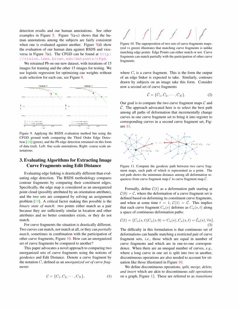
Figure 9. Applying the BSDS evaluation method but using theCFGD ground truth comparing the Third Order Edge Detec-tion [24] (green), and the Pb edge detection retrained on this formof data (red). Left: fine scale annotations, Right: coarse scale an-notations.

3. Evaluating Algorithms for Extracting ImageCurve Fragments using Edit Distance

Evaluating edge linking is drastically different than eval-uating edge detection. The BSDS methodology comparescontour fragments by comparing their constituent edges.Specifically, the edge map is considered as an unorganizedpoint cloud (possibly attributed by an orientation attribute),and the two sets are compared by solving an assignmentproblem [19]. A critical factor making this possible is thebinary state of match: two points either match as a pairbecause they are sufficiently similar in location and otherattributes and no better contenders exists, or they do notmatch.

For curve fragments the situation is drastically different.Two curves can match, not match at all, or they can partiallymatch, sometimes in combination with the participation ofother curve fragments, Figure 10. How can an unorganizedset of curve fragments be compared to another?

This paper advocates a novel approach to comparing twounorganized sets of curve fragments using the notions ofgeodesics and Edit Distance. Denote a curve fragment bythe notation C, defined as an unorganized set of curve frag-ments

C = {C1, C2, · · · , CN}, (1)

Figure 10. The superposition of two sets of curve fragments maps:(red vs green) illustrates that matching curve fragments is unlikematching edge points: Edge Points can either match or not. Curvefragments can match partially with the participation of other curvefragments.

where Ci is a curve fragment. This is the form the outputof an edge linker is expected to take. Similarly, contoursdrawn by subjects on an image take this form. Considernow a second set of curve fragments

C = {C1, C2, · · · , CN}. (2)

Our goal is to compare the two curve fragment maps C andC. The approach advocated here is to select the best pathamong all paths of deformation that incrementally changecurves in one curve fragment set to bring it into register tocorresponding curves in a second curve fragment set, Fig-ure 11.

Figure 11. Compute the geodesic path between two curve frag-ment maps, each path of which is represented as a point. Thered path shows the minimum distance among all deformation se-quences from curve fragment map C to curve fragment map C.

Formally, define C(t) as a deformation path starting atC(0) = C, where the deformation of a curve fragment set isdefined based on deforming its constituent curve fragments,and when at some time t = 1, C(1) = C. This impliesthat each curve fragment Cn(s) deforms as Cn(s, t) alonga space of continuous deformation paths:

C(t) = {Cn(s, t)|Cn(s, 0) = Cn(s), Cn(s, t) = Cn(s),∀n}.(3)

The difficulty in this formulation is that continuous set ofdeformations can handle matching a restricted pair of curvefragment sets, i.e., those which are equal in number ofcurve fragments and which are in one-to-one correspon-dence. When there are an unequal number of curves, e.g.,where a long curve in one set is split into two in another,discontinuous operations are also needed to account for sit-uation like those illustrated in Figure 10.

We define discontinuous operations, split, merge, delete,and insert which are akin to discontinuous edit operationson a graph, Figure 12. These are referred to as transitions

(a) (b) (c) (d) (e)Figure 12. Curve Fragment Map Transitions: (a) Merge, (b) Split,(c) Insert, (d) Purge. These are complemented by continuous de-formation shown in (e). Any curve fragment map can be trans-formed to be in correspondence to another curve fragment mapthrough a sequence of continuous deformations connected by atransitions.

because continuous paths of deformations are connected atthese points, which represent a transition from one contin-uous deformation to another. For example, consider twocurve fragments with a gap between them, Figure 13. Letone curve elongate to cover the gap and then touch the othercurve. Before the two curves can become a long curve inthe deformation process, a merge transition must put themtogether. The set of allowable deformations on a curve frag-ment set are therefore twofold: (i) continuous deformationsand (ii) discontinuous transitions.

(a) (b)Figure 13. (a) Left side C and right side C are two transform se-quence. It shows how Geodesic Distance measure cost deformingC into C. (b) The cost of deformation in this case is DE + FG + HI.

The distance between two sets of curve fragments is thenmeasured as the cost of the geodesic path in this space of de-formations. The computation of distance requires resolvingtwo issues, however: (i) What is the cost of each path, and(ii) how to search an enormously large search space. Eachissue is addressed in turn.

First, the cost of an operation is the likelihood of the datathat is being removed or hallucinated. For the purpose of il-lustration, suppose each set of curve fragments consists ofa single curve. Since the two curves have a common sourcein the image, proximity of matching curves to each othermatters more than the shape of the curves. Since the pro-cess of extracting a curve has an intrinsic level of error,whether it is done by a human in a ground truth markingprocess or by an algorithm, lateral variation in a curve canonly be a limited small distance from its true locations. Thisdistance τd is a system parameter which is set to two pix-els for all experiments shown here. Two curves which aremore than this distance apart cannot match. Similarly, apair of matching curves need to match in orientation, notexceeding an orientation threshold τθ, which is set to 72o

throughout this paper. This is in fact a form of establishing

a minimum Chamfer Distance requirement for two curvesto match. Observe that two curves can potentially matchonly for a limited portion of their length.

The spatial and orientation restriction of potentiallymatching curves implies that the only deformations a curvefragment is allowed to make is to lengthen or shorten. Wecall this continuous deformation process a “deform” and itscost is simply the length change, assuming a uniform dis-tribution over length. The cost of all other operations arebased on the deform cost: a delete operation shrinks a curveto a point and then the point disappears, costing the lengthof the curve1. Conversely, an insert operation generates apoint at no cost and then lengthens this point to the desiredcurve, costing the length of the curve. Similarly, two abut-ting curves are merged at the cost of one pixel, representingthe pixel that is being lengthened or shortened to merge orsplit, respectively.

Second, the issue of searching a rather large space ofpaths is addressed in two steps. The first step followsthe standard string edit distance analogy: there are nu-merous insert/split possibilities while there relatively fewerdelete/merge possibilities. Thus, it is significantly more ef-ficient to break the path from one set of curve fragments toanother into an equivalent pair of subpaths each from a setof curve fragments and culminating on a common simplerset of curve fragments, where each subpath allows deletesand merges but not inserts and splits.

(a) (b)

(c)Figure 14. The grouping of curve fragments into mutually pairedsubsets is illustrated. (a) Human Ground truth. (b) Curve frag-ment extraction. (c) Each group of curve fragments is coloredsimilarly with curves from one set shown in one certain color andthe other in the corresponding darker color. While the isolateddark red curve fragments are the missed ones from human groundtruth, the isolate dark green contours are the extra curve fragmentsgenerated from curve fragment extraction. All Figures are scalableand zooming in helps probe the grouping.

The second step restricts the search space by consider-

1More generally contrast can be incorporated into this cost, but this hasnot been done here.

ing curves only in the τd−neighborhood around each curve.This allows for partitioning the curve fragment sets in mu-tually pairing subsets so that the edit distance need onlybe solved within these sets. The process is illustrated inFigure 15(a). Consider some curve Ci in the first set ofcurve fragments and denote a curve Ci in the second set ofcurve fragments that falls in the τd−neighborhood aroundCi. Refer to this process as pairing Ci and Ci . Sincethis relationship is not one to one, we seek mutually pairingsubsets of curve fragments Cj = {Ci1, Ci2, · · · , CNj

} andCj = {Ci1, Ci2, · · · , CNj

} such that each curve fragmentin Cj has all its paired curves in Cj and vice versa. It mightappear that his kind of chaining might go on for a while, butthe process typically converges rather rapidly. Figure 14shows the subsets Cj and Cj comparing two sets of curvefragments.

(a) (b)

(c) (d)Figure 15. (a) Consider two contour fragments sets are shown inred (c1, c2) and the other in green (c3, c4, c5). The search for mu-tually paring subsets begin with any contour, say c1, and checkingpotential parings in the second set of contour fragments, c3 andc4, in this case. The pairing of each of these contour fragmentsis in turn found in the first set, adding c2 to the group, and thenc5 is added in another iteration. (b) Each contour’s neighborhoodregion is the span area with θ = 60o, radius R = 10, starting 2pixels backward the end point. Mergable curves should have endpoints within each other’s neighborhood without other curves ly-ing within the intersection of neighborhood regions (yellow). (c)Mergable fragment subsets. (d) The minimum cost combination isfound to be {c1, c2, c4}, and {c6, c7, c8}.

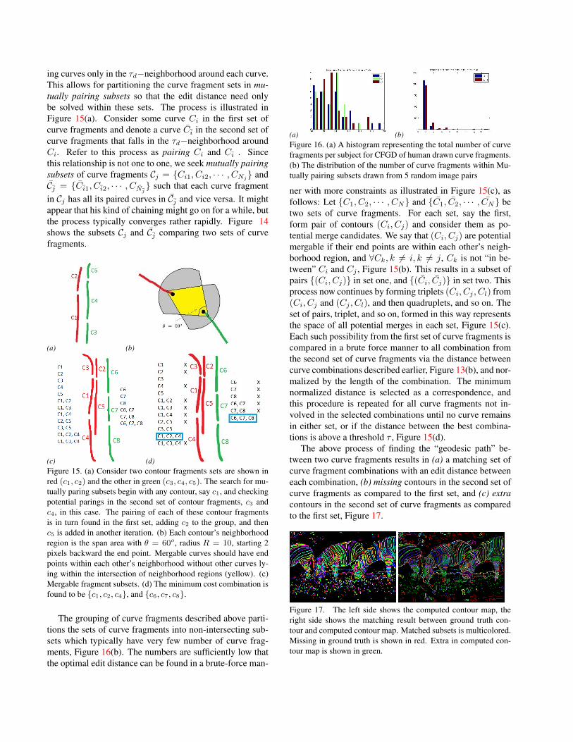
The grouping of curve fragments described above parti-tions the sets of curve fragments into non-intersecting sub-sets which typically have very few number of curve frag-ments, Figure 16(b). The numbers are sufficiently low thatthe optimal edit distance can be found in a brute-force man-

(a) (b)Figure 16. (a) A histogram representing the total number of curvefragments per subject for CFGD of human drawn curve fragments.(b) The distribution of the number of curve fragments within Mu-tually pairing subsets drawn from 5 random image pairs

ner with more constraints as illustrated in Figure 15(c), asfollows: Let {C1, C2, · · · , CN} and {C1, C2, · · · , CN} betwo sets of curve fragments. For each set, say the first,form pair of contours (Ci, Cj) and consider them as po-tential merge candidates. We say that (Ci, Cj) are potentialmergable if their end points are within each other’s neigh-borhood region, and ∀Ck, k 6= i, k 6= j, Ck is not “in be-tween” Ci and Cj , Figure 15(b). This results in a subset ofpairs {(Ci, Cj)} in set one, and {(Ci, Cj)} in set two. Thisprocess now continues by forming triplets (Ci, Cj , Cl) from(Ci, Cj and (Cj , Cl), and then quadruplets, and so on. Theset of pairs, triplet, and so on, formed in this way representsthe space of all potential merges in each set, Figure 15(c).Each such possibility from the first set of curve fragments iscompared in a brute force manner to all combination fromthe second set of curve fragments via the distance betweencurve combinations described earlier, Figure 13(b), and nor-malized by the length of the combination. The minimumnormalized distance is selected as a correspondence, andthis procedure is repeated for all curve fragments not in-volved in the selected combinations until no curve remainsin either set, or if the distance between the best combina-tions is above a threshold τ , Figure 15(d).

The above process of finding the “geodesic path” be-tween two curve fragments results in (a) a matching set ofcurve fragment combinations with an edit distance betweeneach combination, (b) missing contours in the second set ofcurve fragments as compared to the first set, and (c) extracontours in the second set of curve fragments as comparedto the first set, Figure 17.

Figure 17. The left side shows the computed contour map, theright side shows the matching result between ground truth con-tour and computed contour map. Matched subsets is multicolored.Missing in ground truth is shown in red. Extra in computed con-tour map is shown in green.

Figure 18. PR curves of curve extracting systems evaluated on finescale CFGD (left) and coarse scale CFGD (right).

4. ResultsBefore comparing curve fragments, we select the

optimized edge detection threshold using BSDS evaluationmethod on our ground truth dataset. Retrained Pb andthird order edge detector with optimized threshold providesbaselines for edge linkers. The approach for comparingtwo curve fragment sets together with human groundtruth which is in the form of curve fragments allows forthe evaluation of edge linking algorithms, specifically,the generic proximity linker, the Kovasi linker [17], thesymbolic linker [24], and the Van Duc topographicalcontour extraction [23], Figure 18. All linkers are testedon both the Pb edge map [19] as well as on the third-order(TO) edge map [24], except the Van Duc algorithm whereedge detection and linking is integrated. The results showthat symbolic linker performs best when using either Pb orTO edge maps.

Acknowledgments: The support of NSF grant 1116140 isgratefully acknowledged. We also thank Prof. Fowlkes forproviding input and data, and Maruthi Narayanan for tech-nical assistance.

References[1] S. Alpert, M. Galun, B. Nadler, and R. Basri. Detecting faint

curved edges in noisy images. In ECCV’10, pages 750–763,2010. 1

[2] P. Arbelaez. Boundary extraction in natural images usingultrametric contour maps. In CVPRW ’06, page 182, 2006. 2

[3] P. Arbelaez, M. Maire, C. Fowlkes, and J. Malik. Con-tour detection and hierarchical image segmentation. PAMI,33(5):898–916, 2011. 2

[4] S. Borra and S. Sarkar. A framework for performance char-acterization of intermediate-level grouping modules. PAMI,19(11):1306–1312, 1997. 1, 2

[5] K. Bowyer, C. Kranenburg, and S. Dougherty. Edge detectorevaluation using empirical ROC curves. CVIU, 84(1):77–103, 2001. 1

[6] P. Dollar, Z. Tu, and S. Belongie. Supervised learning ofedges and object boundaries. In CVPR’06, pages 1964–1971, 2006. 1, 2

[7] R. Fabbri and B. B. Kimia. 3D curve sketch: Flexible curve-based stereo reconstruction and calibration. In CVPR’10,San Francisco, California, USA, 2010. 2

[8] P. Felzenszwalb and D. McAllester. A min-cover approachfor finding salient curves. In CVPRW ’06, page 185, 2006.1, 2

[9] C. Fowlkes, D. Martin, and J. Malik. Berkeley segmenta-tion dataset and benchmark. www.cs.berkeley.edu/projects/vision/grouping/segbench/. 2

[10] P. Huggins and S. Zucker. Folds and cuts: How shadingflows into edges. In ICCV’01, pages II: 153–158, Vancouver,Canada, July 9-12 2001. 3

[11] L. A. Iverson and S. W. Zucker. Logical/linear operators forimage curves. PAMI, 17(10):982–996, October 1995. 1

[12] V. Jain and B. B. Kimia. Enriched edge-map composite byperceptual fusion of video edge-maps. In ICCVW’07 on Dy-namical Vision, Rio de Janeiro, Brazil, October 2007. 2

[13] V. Jain, B. B. Kimia, and J. L. Mundy. Background modelingbased on subpixel edges. In ICIP’07, volume IV, pages 321–324, San Antonio, TX, USA, September 2007. IEEE. 2

[14] V. Jain, B. B. Kimia, and J. L. Mundy. Segregation of movingobjects using elastic matching. CVIU, 108:230–242, 2007. 2

[15] J. J. Koenderink. What does the occluding contour tell usabout solid shape? Perception, 13:321–330, 1984. 2, 3

[16] J. J. Koenderink and A. J. van Doorn. The shape of smoothobjects and the way contours end. Perception, 11:129–137,1982. 2, 3

[17] P. D. Kovesi. MATLAB and Octave functions for com-puter vision and image processing. Available from:<http://www.csse.uwa.edu.au/∼pk/research/matlabfns/>. 8

[18] M. Maire, P. Arbelaez, C. Fowlkes, and J. Malik. Using con-tours to detect and localize junctions in natural images. InCVPR’08, 2008. 1, 2

[19] D. Martin, C. Fowlkes, and J. Malik. Learning to detect nat-ural image boundaries using local brightness, color, and tex-ture cues. PAMI, 26(5):530–549, 2004. 1, 5, 8

[20] D. Martin, C. Fowlkes, D. Tal, and J. Malik. A databaseof human segmented natural images and its application toevaluating segmentation algorithms and measuring ecologi-cal statistics. ICCV, 2:416–423, 2001. 1, 2

[21] P. Parent and S. W. Zucker. Trace inference, curvature con-sistency and curve detection. PAMI, 11(8):823–839, 1989.1

[22] X. Ren. Multi-scale improves boundary detection in natu-ral images. In ECCV (2), volume 5303 of Lecture Notes inComputer Science, pages 533–545. Springer, 2008. 2

[23] C. Rothwell, J. Mundy, W. Hoffman, and V.-D. Nguyen.Driving vision by topology. In ISCV, pages 395–400, 1995.8

[24] A. Tamrakar and B. B. Kimia. No grouping left behind:From edges to curve fragments. In ICCV ’07, 2007. 5, 8

[25] Z. Tu and S.-C. Zhu. Parsing images into regions, curves,and curve groups. IJCV, 69(2):223–249, Aug. 2006. 1

[26] Q. Zhu, G. Song, and J. Shi. Untangling cycles for contourgrouping. In ICCV’07, pages 1 –8, 2007. 1