recovering low frequencies for impedance inversion by

Low frequency recovering

CREWES Research Report — Volume 25 (2013) 1

Recovering low frequencies for impedance inversion by frequency domain deconvolution

Sina Esmaeili and Gary F. Margrave

ABSTRACT

Acoustic impedance is a rock property that can be derived from seismic data and contains important information about subsurface properties. Direct measurements of acoustic impedance are available from acoustic and density well logs, but these well data can provide the acoustic impedance only at the well’s location. Mathematically it is true that acoustic impedance can be calculated from earth’s reflectivity function, and this function can be estimated from seismic data. Additionally, estimation of reflectivity from seismic data is always bandlimited and affects acoustic impedance significantly. Acoustic impedance inversion can easily be computed by a standard impedance inversion algorithm which uses well logs to fill in the low-frequency information that is missing in bandlimited seismic data.

In this study we investigate the performance of standard deconvolution and its ability to recover low frequency content directly from seismic data. We find that standard deconvolution does not perform well at low frequencies and this is a limiting factor in impedance inversion. Using frequency domain deconvolution, we show that improving the spectral smoothing process and applying a minimum phase spectral color operator to the deconvolved seismic trace can improve the performance of impedance inversion and reduce the bandwidth necessary from well control.

INTRODUCTION

The ultimate goal of geophysics is to determine the earth’s reflectivity as a function of position beneath a seismic survey. Once the raw data is processed, it is possible to estimate the earth’s reflectivity from them. The low frequency seismic data is getting contaminated with low frequency noises, and it will result in missing low frequency data in the recorded data. The question is, can we otherwise suppress low-frequency noise without wasting good information? Waters (1978) described an impedance inversion scheme which is a simple approach to derive impedance values from seismic data. An impedance estimate, from a well log or stacking velocities, is first combined with integrated seismic data in the frequency domain. Detailed impedance values are thus provided by the integrated seismic data, and the low-frequency trend is provided by the well-log. Lindseth (1979) also added low frequencies derived from velocity analysis, and Oldenburg et al. (1983) introduced two different approaches for recovering low frequency information. Acoustic impedance inversion can also be computed easily by a BLIMP (BandLimited IMPedance) algorithm (Ferguson & Margrave, 1996) which uses well logs to fill in the low frequency information that is missing in bandlimited seismic data. Recovering the low frequencies before passing through the impedance estimation process can be challenging. The key point of this idea is estimating the wavelet as accurately as possible during deconvolution hence the low frequency part can be recovered from estimated reflectivity. We start by reintroducing the convolutional model for normal incident seismograms and then show how reflectivity can be estimated by

Esmaeili and Margrave

2 CREWES Research Report — Volume 25 (2013)

deconvolution. Two approaches will be discussed for recovering low frequencies in a deconvolution algorithm, and the result of impedance inversion derived from the new deconvolution will be presented.

THEORY

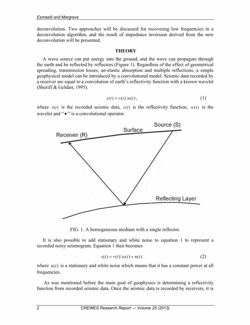
A wave source can put energy into the ground, and the wave can propagate through the earth and be reflected by reflectors (Figure 1). Regardless of the effect of geometrical spreading, transmission losses, an-elastic absorption and multiple reflections, a simple geophysical model can be introduced by a convolutional model. Seismic data recorded by a receiver are equal to a convolution of earth’s reflectivity function with a known wavelet (Sheriff & Geldart, 1995).

( ) ( ) ( )s t r t w t= , (1)

where ( )s t is the recorded seismic data, ( )r t is the reflectivity function, ( )w t is the wavelet and “ • ” is a convolutional operator.

FIG. 1. A homogeneous medium with a single reflector.

It is also possible to add stationary and white noise to equation 1 to represent a recorded noisy seismogram. Equation 1 then becomes

( ) ( ) ( ) ( )s t r t w t n t= + (2)

where ( )n t is a stationary and white noise which means that it has a constant power at all frequencies.

As was mentioned before the main goal of geophysics is determining a reflectivity function from recorded seismic data. Once the seismic data is recorded by receivers, it is



used to estimate reflectivity. However, the only known parameter in equation 2 is ( )s t , which is a function of time, while all other parameters are unknown. Mathematically, deconvolution is an algorithm-based process which is used to reverse the effects of convolution on the recorded data. The goal of a deconvolution scheme is to remove the effect of the wavelet from seismic traces and then retrieving the earth’s reflectivity function. Wiener spiking deconvolution (Leinbach, 1995), maximum entropy (Burg) deconvolution (AuYeung, 1986), frequency domain deconvolution (Margrave, 2002), and Gabor deconvolution (Margrave & Lamoureux, 2002) are different deconvolution methods that can be applied to seismic data to estimate reflectivity. This report outlines an attempt to estimate the reflectivity by applying frequency domain deconvolution to zero-offset seismic data and utilizing the result to calculate acoustic impedance inversion.

Once the reflectivity function has been estimated it is possible to calculate the impedance inversion. The ratio of the amplitude of a reflected wave to the amplitude of the incident wave is called the reflection coefficient, and the function which defines the reflection coefficient for each point in the medium is the reflectivity function. In a one dimensional medium and the acoustic case for the normal incident wavelet, the reflection coefficient can be written as (Margrave, 2002)

1 1

1 1

n n n nn

n n n n

v vrv v

ρ ρρ ρ

+ +

+ +

−=+

, (3)

where 1nρ + and 1nv + are representing density and velocity in the (n+1)th layer respectively,

nρ and nv are density and velocity in the nth layer respectively, and nr is the reflection

coefficient in the nth layer.

The product of density and acoustic velocity, which varies among different rock layers, is known as acoustic impedance, common symbols for it are I and Z. Acoustic impedance indicates how much sound pressure is generated by the vibration of molecules of a particular acoustic medium. Therefore, the equation (3) can be written as

1

1

n nn

n n

I IrI I

+

+

−=+

, (4)

where 1nI + and nI represent the acoustic impedance of the (n+1)th and nth layer

respectively. To calculate the acoustic impedance instead of using the impedance to compute reflection coefficients in equation 4, it is possible to use reflection coefficients which are derived from seismic data, in order to determine acoustic inversion (Lindseth, 1979). The reflection coefficients can be derived from recorded seismic data and well logs. Mathematically, the impedance can be written in terms of reflection coefficients like

1

1

1n

n nn

rI Ir+

+= − . (5)

By assuming 1nr equation (5) can be approximately written as



( )( ) ( ) ( )2

1 1 1 1 1 2n n n n n n n nI I r r I r I r+ = + + + + . (6)

Replacing n by n-1, equation 5 can be written for nI as

( )1 11 2n n nI I r− −+ . (7)

Using the same procedure for upper layers, 1nI + can be rewritten as

( )1 11

1 2n

n jj

I I r+=

= +∏ , (8)

And by a simple calculation, 1 2 jr+ can be estimated as

( ) 21 2 jRjr e+ . (9)

Therefore, equation 8 becomes

( ) 1

22

1 1 11

n

jj j

rnr

nj

I I e I e =+

=

= =∏ (10)

Equation 10 is a type of inversion process which computes acoustic impedance from seismic reflection information and is known as impedance inversion (II). Therefore, given the impedance of the first layer and the estimated reflectivity function, acoustic impedance can be calculated.

We want to know reflectivity with as much precision and resolution as possible for a variety of reasons. As an example, large reflection coefficients may indicate sand layers which are potential hydrocarbon reservoirs. On the other hand, seismic sources do not generate useful power at all frequencies, therefore it is accepted that any reflectivity estimate must be bandlimited. In this situation the bandlimited reflectivity includes fewer details than the actual earth reflectivity. The broadband and bandlimited reflectivity in the frequency and time domain is illustrated in figure 2.



FIG. 2. Comparing broadband and bandlimited reflectivity in both frequency and time domain

The first diagram shows that the broadband reflectivity contains all frequencies from zero to 500 Hz, but the bandlimited one contains only the frequencies from 10 Hz to 120 Hz. In the second diagram, the differences between two reflectivity functions are noticeable. It can be realized that the data which lack low and high frequencies have less resolution than the broadband data set.

Frequency Domain Deconvolution

The method described here is based on a frequency domain framework, which might be the easiest way to estimate reflectivity. Regardless of the phase spectrum of a seismic trace, the amplitude spectrum of seismic data is similar in shape to the amplitude spectrum of wavelet as shown in Figure 3.

FIG. 3. Amplitude spectrum of white spectrum reflectivity (blue), seismic data (green) and a minimum phase wavelet (red).



If the amplitude spectrum of the wavelet can be computed by smoothing the amplitude spectrum of seismic data, the amplitude spectrum of the wavelet could be extracted and thus the reflectivity can be estimated. The perfect deconvolution operator can be defined as:

( ) ( ) ( ),w t d t tδ= (11)

so ( )d t is inverse of ( )w t . By substituting the inverse of ( )w t into equation 1, ( )r t becomes

( ) ( ) ( ),r t s t d t= (12)

where ( )r t is the exact reflectivity function. But in practice, because of the bandlimited nature of wavelets and the unavoidable presence of noise, even if we could find ( )d t as a function to make equation 11 equal to ( )tδ , such an operator would simply produce noise at frequencies where noise dominates signal. This important fact leads us to the concept that the estimated reflectivity function is never exactly the same as the true reflectivity function. Mathematically, it can be written as:

( ) ( ) ( ),d ds t r t w t= (13)

where ( )ds t is the estimated reflectivity, and ( )dw t can be represented as

( ) ( ) ( ),dw t d t w t= (14)

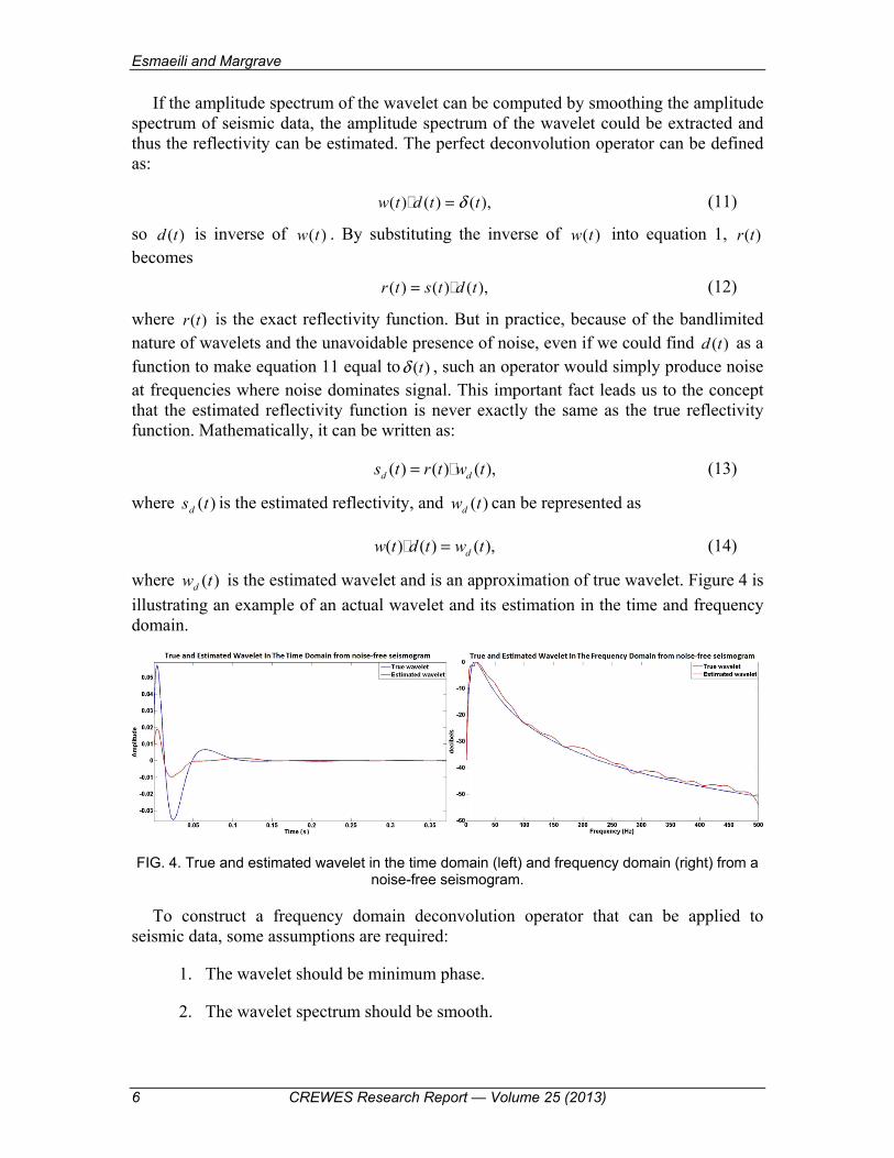
where ( )dw t is the estimated wavelet and is an approximation of true wavelet. Figure 4 is

illustrating an example of an actual wavelet and its estimation in the time and frequency domain.

FIG. 4. True and estimated wavelet in the time domain (left) and frequency domain (right) from a noise-free seismogram.

To construct a frequency domain deconvolution operator that can be applied to seismic data, some assumptions are required:

1. The wavelet should be minimum phase.

2. The wavelet spectrum should be smooth.



3. The wavelet should be stationary.

4. The reflectivity is assumed to be random, therefore its amplitude spectrum is assumed to be white.

On the other hand, by writing equation 2 in frequency domain,

( ) ( ) ( ) ( ),S f R f W f N f= + (15)

It is possible to define a specific region of frequency ( min maxf f f≤ ≤ ), in which the

( ) ( )R f W f term dominates over ( )N f and the noisy and noise-free seismograms are almost the same (figure 5). The white reflectivity assumption means

( ) 1,R f ≈ (16)

where the overbar indicates smoothing. Therefore, the amplitude spectrum of an estimated wavelet can be expressed as

( ) ( ) .S f W f≈ (17)

The amplitude spectrum of a deconvolution operator can be calculated from equation 17 and equation 14 as following

11

( ) ( ) ( ) ,estimated

D f W f S f−−= = (18)

which indicates that the amplitude spectrum of the deconvolution operator is the inverse of the estimated wavelet or inverse of the smoothing of the seismic amplitude spectrum. Therefore, the better smoothing of the seismic data we have the better reflectivity estimation.

FIG. 5. Amplitude spectrum of noisy and noise-free seismograms.

According to the minimum phase assumption of a wavelet and all above results, the complete form of a deconvolution operator becomes (Margrave, 2002)



( )

max

1( ) ,

( )Di f

est

D f eW f A

φ

μ=

+ (19)

where μ is called the stability factor or white noise factor, a small positive number usually between 0.01 and 0.000001, and maxA is the maximum value of the spectrum of

( )est

W f . Also, ( )D fφ is the phase of the deconvolution operator and can be defined as

( ) ( )( )ln ( ) ,D f H D fφ = (20)

where H is a linear transform and is called Hilbert transform. By applying equation 19 to a seismic trace, the reflectivity function can be estimated.

REAL WELL DATA DECONVOLUTION RESULTS

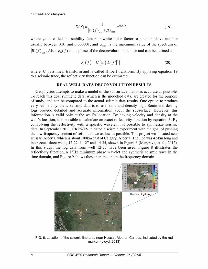
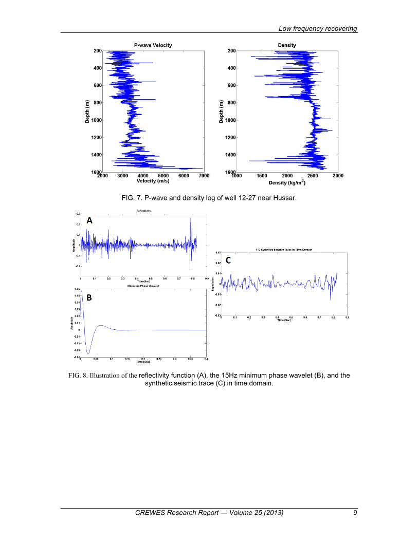
Geophysics attempts to make a model of the subsurface that is as accurate as possible. To reach this goal synthetic data, which is the modelled data, are created for the purpose of study, and can be compared to the actual seismic data results. One option to produce very realistic synthetic seismic data is to use sonic and density logs. Sonic and density logs provide detailed and accurate information about the subsurface. However, this information is valid only at the well’s location. By having velocity and density at the well’s location, it is possible to calculate an exact reflectivity function by equation 3. By convolving the reflectivity with a specific wavelet it is possible to synthesize seismic data. In September 2011, CREWES initiated a seismic experiment with the goal of pushing the low-frequency content of seismic down as low as possible. This project was located near Hussar, Alberta, which is about 100km east of Calgary, Alberta. The line was 4.5km long and intersected three wells, 12-27, 14-27 and 14-35, shown in Figure 6 (Margrave, et al., 2012). In this study, the log data from well 12-27 have been used. Figure 8 illustrates the reflectivity function, a 15Hz minimum phase wavelet and synthetic seismic trace in the time domain, and Figure 9 shows these parameters in the frequency domain.

FIG. 6. Location of the seismic line area near Hussar, Alberta, Canada, indicated by the red marker. (Lloyd, 2013)



FIG. 7. P-wave and density log of well 12-27 near Hussar.

FIG. 8. Illustration of the reflectivity function (A), the 15Hz minimum phase wavelet (B), and the synthetic seismic trace (C) in time domain.



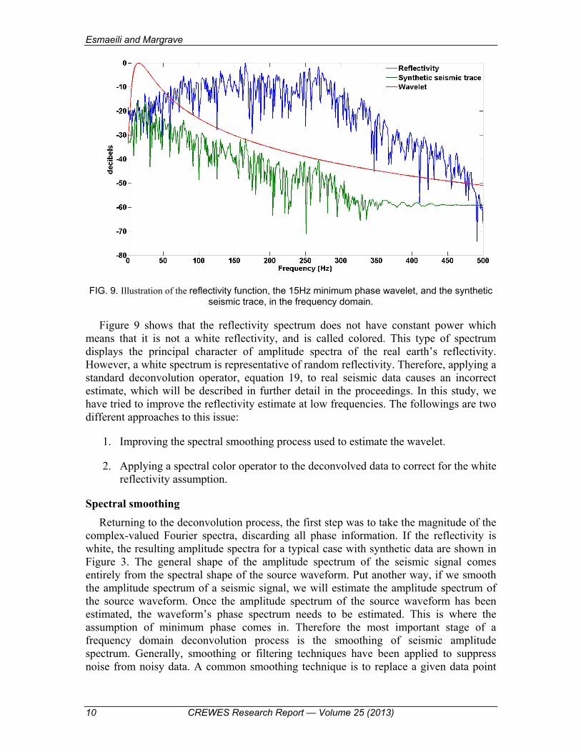
FIG. 9. Illustration of the reflectivity function, the 15Hz minimum phase wavelet, and the synthetic seismic trace, in the frequency domain.

Figure 9 shows that the reflectivity spectrum does not have constant power which means that it is not a white reflectivity, and is called colored. This type of spectrum displays the principal character of amplitude spectra of the real earth’s reflectivity. However, a white spectrum is representative of random reflectivity. Therefore, applying a standard deconvolution operator, equation 19, to real seismic data causes an incorrect estimate, which will be described in further detail in the proceedings. In this study, we have tried to improve the reflectivity estimate at low frequencies. The followings are two different approaches to this issue:

1. Improving the spectral smoothing process used to estimate the wavelet.

2. Applying a spectral color operator to the deconvolved data to correct for the white reflectivity assumption.

Spectral smoothing

Returning to the deconvolution process, the first step was to take the magnitude of the complex-valued Fourier spectra, discarding all phase information. If the reflectivity is white, the resulting amplitude spectra for a typical case with synthetic data are shown in Figure 3. The general shape of the amplitude spectrum of the seismic signal comes entirely from the spectral shape of the source waveform. Put another way, if we smooth the amplitude spectrum of a seismic signal, we will estimate the amplitude spectrum of the source waveform. Once the amplitude spectrum of the source waveform has been estimated, the waveform’s phase spectrum needs to be estimated. This is where the assumption of minimum phase comes in. Therefore the most important stage of a frequency domain deconvolution process is the smoothing of seismic amplitude spectrum. Generally, smoothing or filtering techniques have been applied to suppress noise from noisy data. A common smoothing technique is to replace a given data point



with the mean value of points in its neighborhood. The size of the “neighborhood” defines the size of the smoothing operator. An equally whitened local average is achieved by convolving the spectrum with a boxcar function. This process naturally results in a smoother signal. In this study, we investigate the use of a Gaussian smoother instead of a boxcar smoother.

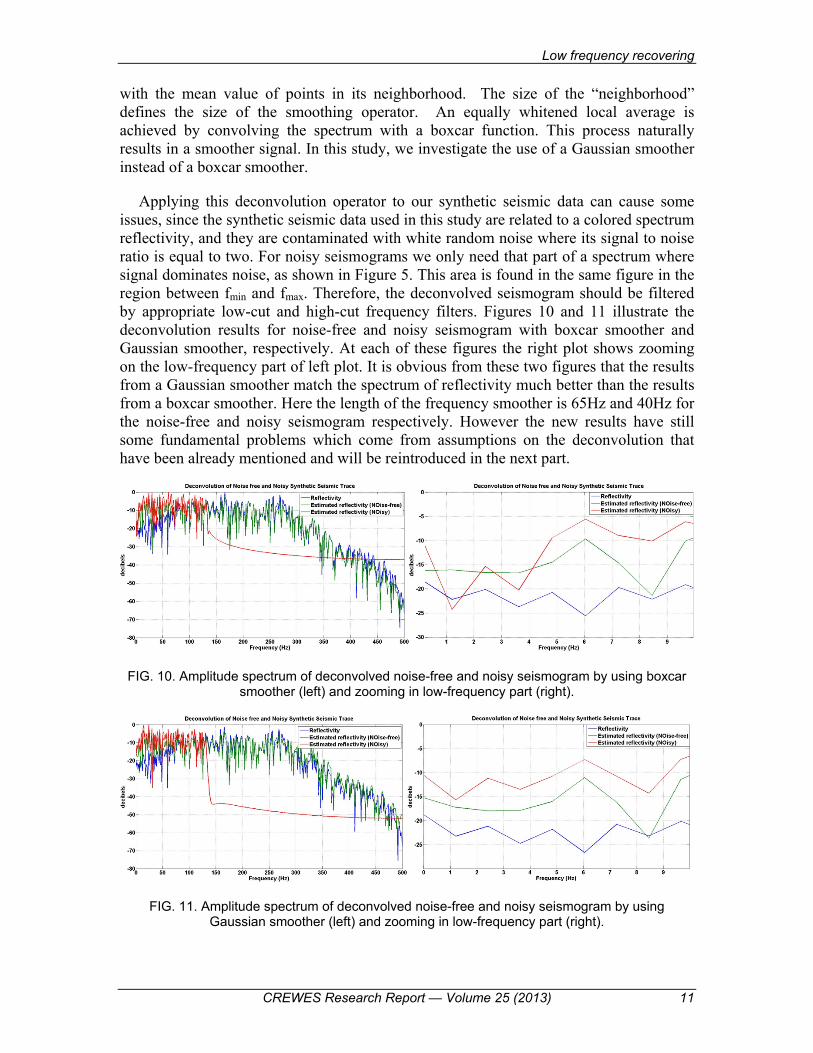
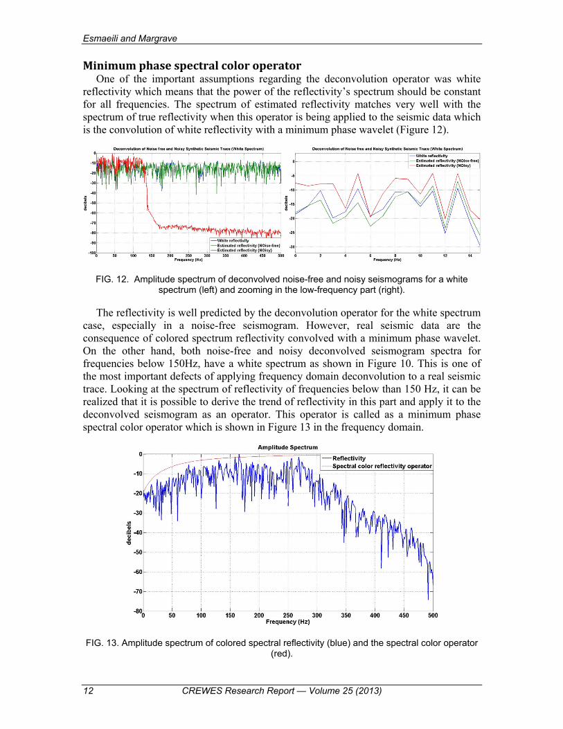
Applying this deconvolution operator to our synthetic seismic data can cause some issues, since the synthetic seismic data used in this study are related to a colored spectrum reflectivity, and they are contaminated with white random noise where its signal to noise ratio is equal to two. For noisy seismograms we only need that part of a spectrum where signal dominates noise, as shown in Figure 5. This area is found in the same figure in the region between fmin and fmax. Therefore, the deconvolved seismogram should be filtered by appropriate low-cut and high-cut frequency filters. Figures 10 and 11 illustrate the deconvolution results for noise-free and noisy seismogram with boxcar smoother and Gaussian smoother, respectively. At each of these figures the right plot shows zooming on the low-frequency part of left plot. It is obvious from these two figures that the results from a Gaussian smoother match the spectrum of reflectivity much better than the results from a boxcar smoother. Here the length of the frequency smoother is 65Hz and 40Hz for the noise-free and noisy seismogram respectively. However the new results have still some fundamental problems which come from assumptions on the deconvolution that have been already mentioned and will be reintroduced in the next part.

FIG. 10. Amplitude spectrum of deconvolved noise-free and noisy seismogram by using boxcar smoother (left) and zooming in low-frequency part (right).

FIG. 11. Amplitude spectrum of deconvolved noise-free and noisy seismogram by using Gaussian smoother (left) and zooming in low-frequency part (right).



Minimum phase spectral color operator One of the important assumptions regarding the deconvolution operator was white

reflectivity which means that the power of the reflectivity’s spectrum should be constant for all frequencies. The spectrum of estimated reflectivity matches very well with the spectrum of true reflectivity when this operator is being applied to the seismic data which is the convolution of white reflectivity with a minimum phase wavelet (Figure 12).

FIG. 12. Amplitude spectrum of deconvolved noise-free and noisy seismograms for a white spectrum (left) and zooming in the low-frequency part (right).

The reflectivity is well predicted by the deconvolution operator for the white spectrum case, especially in a noise-free seismogram. However, real seismic data are the consequence of colored spectrum reflectivity convolved with a minimum phase wavelet. On the other hand, both noise-free and noisy deconvolved seismogram spectra for frequencies below 150Hz, have a white spectrum as shown in Figure 10. This is one of the most important defects of applying frequency domain deconvolution to a real seismic trace. Looking at the spectrum of reflectivity of frequencies below than 150 Hz, it can be realized that it is possible to derive the trend of reflectivity in this part and apply it to the deconvolved seismogram as an operator. This operator is called as a minimum phase spectral color operator which is shown in Figure 13 in the frequency domain.

FIG. 13. Amplitude spectrum of colored spectral reflectivity (blue) and the spectral color operator (red).



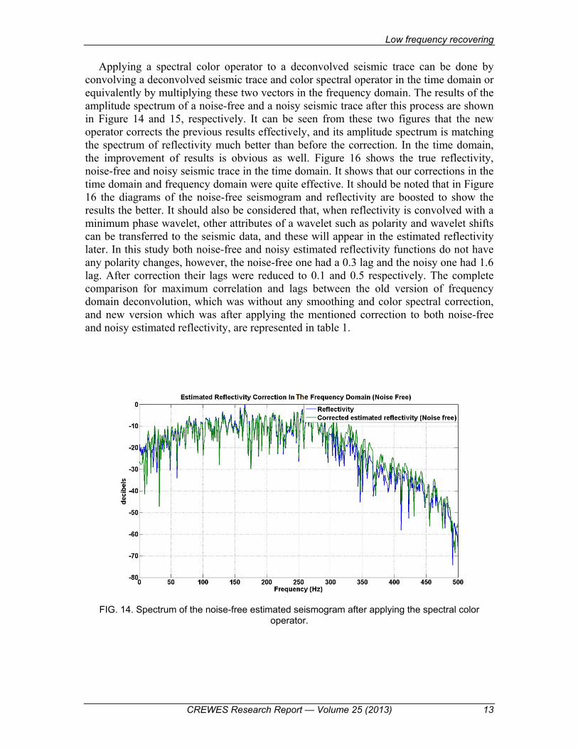
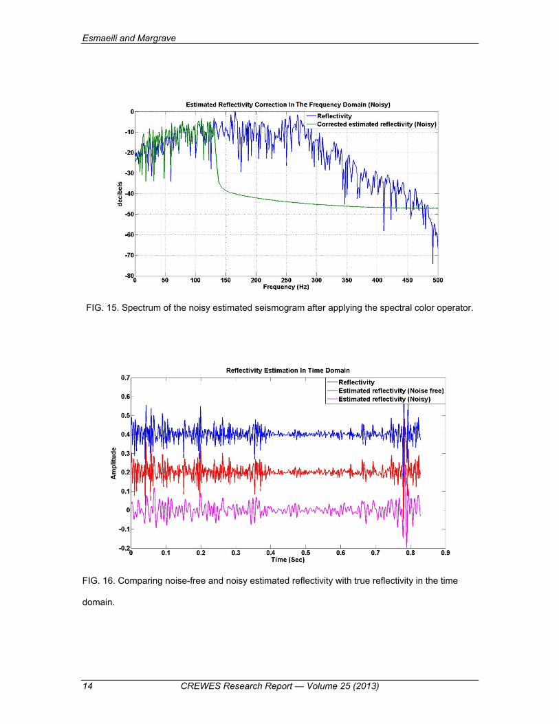
Applying a spectral color operator to a deconvolved seismic trace can be done by convolving a deconvolved seismic trace and color spectral operator in the time domain or equivalently by multiplying these two vectors in the frequency domain. The results of the amplitude spectrum of a noise-free and a noisy seismic trace after this process are shown in Figure 14 and 15, respectively. It can be seen from these two figures that the new operator corrects the previous results effectively, and its amplitude spectrum is matching the spectrum of reflectivity much better than before the correction. In the time domain, the improvement of results is obvious as well. Figure 16 shows the true reflectivity, noise-free and noisy seismic trace in the time domain. It shows that our corrections in the time domain and frequency domain were quite effective. It should be noted that in Figure 16 the diagrams of the noise-free seismogram and reflectivity are boosted to show the results the better. It should also be considered that, when reflectivity is convolved with a minimum phase wavelet, other attributes of a wavelet such as polarity and wavelet shifts can be transferred to the seismic data, and these will appear in the estimated reflectivity later. In this study both noise-free and noisy estimated reflectivity functions do not have any polarity changes, however, the noise-free one had a 0.3 lag and the noisy one had 1.6 lag. After correction their lags were reduced to 0.1 and 0.5 respectively. The complete comparison for maximum correlation and lags between the old version of frequency domain deconvolution, which was without any smoothing and color spectral correction, and new version which was after applying the mentioned correction to both noise-free and noisy estimated reflectivity, are represented in table 1.

FIG. 14. Spectrum of the noise-free estimated seismogram after applying the spectral color operator.



FIG. 15. Spectrum of the noisy estimated seismogram after applying the spectral color operator.

FIG. 16. Comparing noise-free and noisy estimated reflectivity with true reflectivity in the time

domain.



Frequency Domain Deconvolution (Boxcar smoother before applying

color spectral operator)

Frequency Domain Deconvolution (Gaussian smoother after applying

color spectral operator )

Estimated reflectivity (Noise-free)

Maximum Correlation = 0.8668

Lag = 0.2000


Lag = 0.3000

Estimated reflectivity (Noisy)


Lag = 1.4000


Lag = 0.5000

Table 1. Table of maximum correlation between estimated reflectivity and true reflectivity in two different cases.

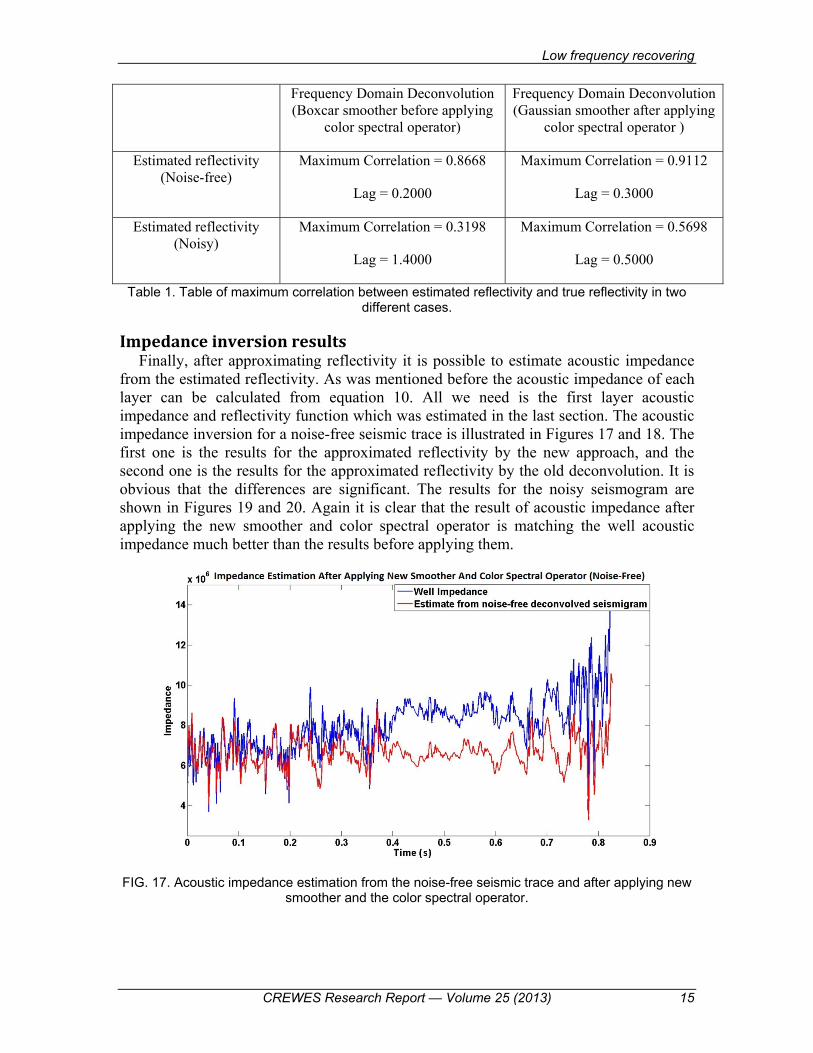
Impedance inversion results Finally, after approximating reflectivity it is possible to estimate acoustic impedance

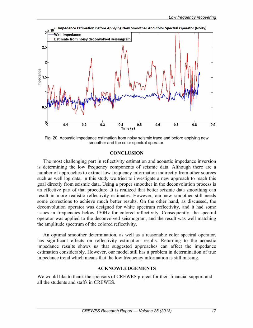
from the estimated reflectivity. As was mentioned before the acoustic impedance of each layer can be calculated from equation 10. All we need is the first layer acoustic impedance and reflectivity function which was estimated in the last section. The acoustic impedance inversion for a noise-free seismic trace is illustrated in Figures 17 and 18. The first one is the results for the approximated reflectivity by the new approach, and the second one is the results for the approximated reflectivity by the old deconvolution. It is obvious that the differences are significant. The results for the noisy seismogram are shown in Figures 19 and 20. Again it is clear that the result of acoustic impedance after applying the new smoother and color spectral operator is matching the well acoustic impedance much better than the results before applying them.

FIG. 17. Acoustic impedance estimation from the noise-free seismic trace and after applying new smoother and the color spectral operator.



FIG. 18. Acoustic impedance estimation from the noise-free seismic trace and before applying new smoother and the color spectral operator.

FIG. 19. Acoustic impedance estimation from noisy seismic traces and after applying new smoother and the color spectral operator.



Fig. 20. Acoustic impedance estimation from noisy seismic trace and before applying new smoother and the color spectral operator.

CONCLUSION

The most challenging part in reflectivity estimation and acoustic impedance inversion is determining the low frequency components of seismic data. Although there are a number of approaches to extract low frequency information indirectly from other sources such as well log data, in this study we tried to investigate a new approach to reach this goal directly from seismic data. Using a proper smoother in the deconvolution process is an effective part of that procedure. It is realized that better seismic data smoothing can result in more realistic reflectivity estimates. However, our new smoother still needs some corrections to achieve much better results. On the other hand, as discussed, the deconvolution operator was designed for white spectrum reflectivity, and it had some issues in frequencies below 150Hz for colored reflectivity. Consequently, the spectral operator was applied to the deconvolved seismogram, and the result was well matching the amplitude spectrum of the colored reflectivity.

An optimal smoother determination, as well as a reasonable color spectral operator, has significant effects on reflectivity estimation results. Returning to the acoustic impedance results shows us that suggested approaches can affect the impedance estimation considerably. However, our model still has a problem in determination of true impedance trend which means that the low frequency information is still missing.

ACKNOWLEDGEMENTS

We would like to thank the sponsors of CREWES project for their financial support and all the students and staffs in CREWES.



REFERENCES

AuYeung, C. (1986). Maximum entropy deconvolution. IEEE International Conference

on ICASSP '86. (Volume:11 ) , (pp. 273 - 276 ). Ferguson, R. J., & Margrave, G. F. (1996). A simple algorithm for bandlimited

impedance inversion. CREWES research report, Vol. 8, No. 21. Leinbach, J. (1995). Wiener spiking deconvolution and minimum-phase wavelets: A

tutorial. Geophysics. Lindseth, R. O. (1979). Synthetic sonic logs-a process for stratigraphic interpretation.

Geophysics, 3-26. Lloyd, H. E. (2013). An Investigation of the Role of Low Frequencies in Seismic

Impedance Inversion. Calgary: University of Calgary. Margrave, G. F. (2002). Methods of seismic data processing. Calgary: Department of

Geoscience, University of Calgary. Margrave, G. F., & Lamoureux, M. P. (2002). Gabor deconvolution. CSEG Geophysics. Margrave, G. F., Mewhort, L., Phillips, T., Hall, M., Bertram, M. B., Lawton, D. C., et al.

(2012). The Hussar low-frequency experiment. CSEG Recorder, Sept., 25-39. Oldenburg, D. W., Scheuer, T., & Levy, S. (1983). Recovery of the acoustic impedance

from reflection seismograms. Geophysics, 1318-1337. Sheriff, R. E., & Geldart, L. P. (1995). Exploration Seismology. Cambridge University

Press. Waters, K. H. (1978). Reflection seismology, a tool for energy resource exploration. New

York: John Wiley and Sons.

recovering low frequencies for impedance inversion by

Documents