modelling the uncertainty in recovering articulation from acoustics

Modelling the uncertainty in recovering articulationfrom acoustics

Korin Richmond *, Simon King, Paul Taylor

Centre for Speech Technology Research, University of Edinburgh, 2 Buccleuch Place, Edinburgh EH8 9LW, UK

Abstract

This paper presents an experimental comparison of the performance of the multilayer perceptron (MLP)with that of the mixture density network (MDN) for an acoustic-to-articulatory mapping task. A corpus ofacoustic-articulatory data recorded by electromagnetic articulography (EMA) for a single speaker was usedas training and test data for this purpose. In theory, the MDN is able to provide a richer, more �exibledescription of the target variables in response to a given input vector than the least-squares trained MLP.Our results show that the mean likelihoods of the target articulatory parameters for an unseen test set wereindeed consistently higher with the MDN than with the MLP. The increase ranged from approximately 3%to 22%, depending on the articulatory channel in question. On the basis of these results, we argue that usinga more �exible description of the target domain, such as that o�ered by the MDN, can prove bene�cialwhen modelling the acoustic-to-articulatory mapping.

1. Introduction

1.1. Background

A successful method for inferring articulation from the acoustic speech signal would �nd manypotential applications: low bit-rate speech coding, helping individuals with speech or hearingimpairment by providing visual feedback during speech training, and the possibility o� mproved

Computer Speech and Language 17 (2003) 153–172

* Corresponding author. Tel.: +44-131-651-1769; fax: +44-131-650-4587.E-mail address: [email protected] (K. Richmond).

automatic speech recognition. Therefore, it is unsurprising that researchers have been investi-gating the acoustic-to-articulatory mapping for several decades.

Much of this work has pursued an analytical approach, whereby an acoustic signal is subjectedto mathematical analysis to yield the area function of a tube model that might have generated it.Many early attempts in particular took this approach. For example, Wakita (1979) attempted toinfer the area functions for a model vocal tract for vowel sounds. Unfortunately, analyticalmethods have struggled with some fundamental difficulties. Certain types of speech sound haveproved more challenging than others, such as where coupling of the nasal and oral cavities occurs.Perhaps most importantly, there is no independent means of assessing the performance of theinversion mapping. Moreover, certain inferred vocal tract configurations may not even bephysiologically possible, let alone common in the speech of human speakers.

Researchers have also turned to articulatory synthesis models for help in studying and devel-oping an inversion mapping. These may be used as part of a ‘‘mimic’’ algorithm, where the modelparameters are iteratively adjusted to minimise cost functions based on the model output and thetarget acoustic signal (e.g., Shirai & Kobayashi, 1986). Synthesis models have also been used togenerate a database of acoustic-articulatory vector pairs by sampling from the domain of thearticulatory control parameters. Such a database can either be used directly for performing theinversion mapping (e.g., Atal, Chang, Mathews, & Tukey, 1978), or as training data for otherempirical learning models. As an example of the latter, Rahim, Goodyear, Kleijn, Schroeter, andSondhi (1993) used Mermelstein�s articulatory model (Mermelstein, 1973) to generate data fortraining various MLPs.

Unfortunately, as with analytical methods, the use of articulatory synthesis models still leavesus with fundamental problems in terms of satisfactory assessment with respect to real humanspeech. It is also conceivable that limitations in either the accuracy or scope of the model itselfcould manifest themselves in a generated data set.

Human articulography data avoids artifacts resulting from limitations and inaccuracies in thegenerating model that might afflict synthetic data. What is more, we are not left with the same dif-ficulties in assessing how an inversionmethod is really performing; we can evaluate the performanceof an inversion algorithm by comparison with how the speaker actually articulated an utterance. Assuch, human articulographic data is a very useful resource for studying the inversion mapping.

Thanks to technologies such as X-ray microbeam (XRMB) cinematography and electromag-netic articulography (EMA), measured human articulatory data has become increasingly acces-sible. However, despite the potential advantages, only a relatively small number of studies whereempirical learning models have been applied to measured articulatory data have been previouslyreported. These include extended Kalman filtering (Dusan, 2000), self-organising HMMs(Roweis, 1999), codebook methods (Hogden et al., 1996), and the MLP (Papcun et al., 1992;Zachs & Thomas, 1994). The studies that have been done have focused almost entirely on a re-stricted set of speech sounds. Therefore, attempting inversion for all speech sounds and forcontinuous speech, as described in the current paper, is a necessary research step in itself.

1.2. Approach to inversion

The MLP is well known as a universal function approximator and has advantages in terms ofefficiency compared with many models. For example, Rahim, Kleijn, Schroeter, and Goodyear

154 K. Richmond et al. / Computer Speech and Language 17 (2003) 153–172

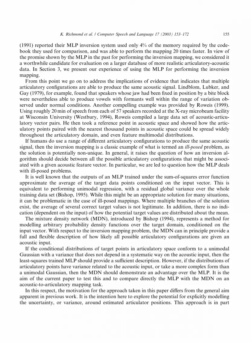
(1991) reported their MLP inversion system used only 4% of the memory required by the code-book they used for comparison, and was able to perform the mapping 20 times faster. In view ofthe promise shown by the MLP in the past for performing the inversion mapping, we considered ita worthwhile candidate for evaluation on a larger database of more realistic articulatory-acousticdata. In Section 3, we present our experience of using the MLP for performing the inversionmapping.

From this point we go on to address the implications of evidence that indicates that multiplearticulatory configurations are able to produce the same acoustic signal. Lindblom, Lubker, andGay (1979), for example, found that speakers whose jaw had been fixed in position by a bite blockwere nevertheless able to produce vowels with formants well within the range of variation ob-served under normal conditions. Another compelling example was provided by Roweis (1999).Using roughly 20min of speech from each of 57 speakers recorded at the X-ray microbeam facilityat Wisconsin University (Westbury, 1994), Roweis compiled a large data set of acoustic-articu-latory vector pairs. He then took a reference point in acoustic space and showed how the artic-ulatory points paired with the nearest thousand points in acoustic space could be spread widelythroughout the articulatory domain, and even feature multimodal distributions.

If humans do use a range of different articulatory configurations to produce the same acousticsignal, then the inversion mapping is a classic example of what is termed an ill-posed problem, asthe solution is potentially non-unique. In general, it raises the question of how an inversion al-gorithm should decide between all the possible articulatory configurations that might be associ-ated with a given acoustic feature vector. In particular, we are led to question how the MLP dealswith ill-posed problems.

It is well known that the outputs of an MLP trained under the sum-of-squares error functionapproximate the average of the target data points conditioned on the input vector. This isequivalent to performing unimodal regression, with a residual global variance over the wholetraining data set (Bishop, 1995). While this might be an appropriate solution for many situations,it can be problematic in the case of ill-posed mappings. Where multiple branches of the solutionexist, the average of several correct target values is not legitimate. In addition, there is no indi-cation (dependent on the input) of how the potential target values are distributed about the mean.

The mixture density network (MDN), introduced by Bishop (1994), represents a method formodelling arbitrary probability density functions over the target domain, conditioned on theinput vector. With respect to the inversion mapping problem, the MDN can in principle provide afull and flexible description of how likely all possible articulatory configurations are given anacoustic input.

If the conditional distributions of target points in articulatory space conform to a unimodalGaussian with a variance that does not depend in a systematic way on the acoustic input, then theleast-squares trained MLP should provide a sufficient description. However, if the distributions ofarticulatory points have variance related to the acoustic input, or take a more complex form thana unimodal Gaussian, then the MDN should demonstrate an advantage over the MLP. It is theaim of the current paper to test this and to compare directly the MLP with the MDN on anacoustic-to-articulatory mapping task.

In this respect, the motivation for the approach taken in this paper differs from the general aimapparent in previous work. It is the intention here to explore the potential for explicitly modellingthe uncertainty, or variance, around estimated articulator positions. This approach is in part

K. Richmond et al. / Computer Speech and Language 17 (2003) 153–172 155

motivated by the view that, if inferred articulation is to provide useful application, we need toknow how much confidence to ascribe to the accuracy of the inferred articulatory parameters ateach point in time.

This paper first introduces the measured articulatory data that has been used in the exper-iments described, and explains how it was processed for use as training data for the neuralnetworks. Next, we describe our implementation of an MLP for performing the inversion taskand evaluate its performance compared with other systems reported in the literature. We thendescribe how MDNs have been applied to the same inversion problem. Finally, the charac-teristics of an MLP and an MDN for performing the acoustic-to-articulatory mapping on thisdata set are compared.

2. The inversion task

2.1. MOCHA

The multichannel articulatory (MOCHA) database has recently been recorded in the purposebuilt studio at the Edinburgh Speech Production Facility at Queen Margaret University College(Wrench & Hardcastle, 2000).

During speech, four data streams were recorded concurrently straight to computer: theacoustic waveform (16 kHz sample rate, with 16 bit precision) together with laryngograph,electropalatograph and electromagnetic articulograph data. The electromagnetic articulographsampled the movement of receiver coils attached to the articulators in the midsagittal plane at500Hz. Coils were affixed to the top lip, bottom lip, bottom incisor, tongue tip, tongue body,tongue dorsum and velum. With each of these sensors providing x- and y-coordinates in themidsagittal plane, 14 channels of salient articulatory information were recorded in total. Addi-tional coils were attached to the bridge of the nose and the upper incisor. However, the signalsfrom these coils, which should have minimal movement relative to each other, were only used toprovide reference points for an algorithm which processed the other EMA channels to correct forhead movement.

The speakers were recorded reading a set of 460 British TIMIT sentences. These short sentenceswere designed to provide phonetically diverse material. They were chosen in an attempt to capturewith good coverage the connected speech processes in English and thus to maximise the usefulnessof the MOCHA database for speech technology and speech science research purposes.

The final release of the database will feature up to 40 speakers with a variety of regional ac-cents. At the time of conducting the experiments described here, two speakers had been madeavailable: one male with a Northern English accent and one female speaker with a SouthernEnglish accent. For this paper, the acoustic waveform and EMA data recorded for the secondspeaker (fsew0) were used.

2.2. Data processing

In order to render the raw articulatory and acoustic data into a format suitable for use withneural networks, several processing steps were carried out. First, filterbank analysis was per-


formed on the acoustic signal, using a Hamming window of 20ms with a shift of 10ms. For eachtime frame, the acoustic vector consisted of 20 melscale filterbank coefficients. These were nor-malised across all 460 utterances to lie within the range ½0:0; 1:0�.

The articulatory feature vector comprised the x- and y-coordinates of the seven EMA sensorcoils. In order to obtain an articulatory feature vector to pair with each acoustic vector, the EMAtraces were downsampled to match the 10ms shift rate of the acoustic feature vectors. Prior todownsampling, the signal was first lowpass filtered with a zero-phase FIR filter to lessen the effectof noise resulting from measurement error in the EMA machine. The articulatory feature vectorswere normalised to lie in the range ½0:1; 0:9�. This range was used because the logistic activationfunction of the output units in the MLP has unrealisable asymptotic limits of 0.0 and 1.0. Allnormalisation was performed as standard, using mean and standard deviation, then shifting andscaling for the data to lie within the desired range. Further details of the normalisation processcan be found in Richmond (2002).

The files for each utterance of speaker fsew0 contain an average of approximately 1.3 s ofsilence in total before and after the utterance. This compares with an average utterance length of2.7 s. During silent stretches, the mouth can potentially take any configuration. This could pose aserious problem to network training, because given an acoustic feature vector representing silence,the network would be attempting to map to a large range of possible articulatory configurations.Therefore, care was taken to omit all data containing silence.

From the 460 utterances contained in the database of speaker fsew0, 368 files were included inthe training set, 46 files in a validation set, while 46 files were put aside for the test set. The fulltraining set contained 92,557 pairs of acoustic and articulatory feature vectors.

3. MLP inversion mapping

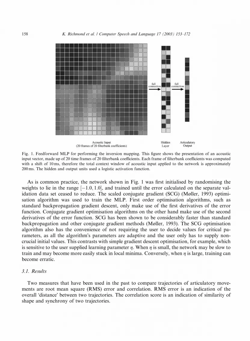
The feedforward MLP used to perform the inversion mapping is shown in Fig. 1. As indicated,this network featured 14 output units, one for each of the x- and y-coordinates of the seven EMAcoil positions. The input layer of the network contained 400 units, which provided a contextwindow of 20 frames of 20 filterbank coefficients each. The use of a context window in theacoustic input domain was similar to the approach of Papcun et al. (1992), and empirical eval-uation has indeed found it to be beneficial (Richmond, 2002).

We used the Skeletonization algorithm (Mozer & Smolensky, 1989) to help identify asuitable number of hidden units. This pruning algorithm works by taking a fully trained MLPand identifying the node whose removal would result in the lowest increase in error on thetraining set. This node is then removed, and the network is further trained to compensate. Thetwo steps of removing the least salient node and then retraining are repeated iteratively untilremoving a further node results in a deficit in network performance that it is not possible torecoup.

In this case, the initial MLP contained 50 hidden units. The best performance was observed inthe network with only 38 units remaining; after this point, the network became progressivelyworse with the removal of each unit. This number of units was corroborated as approximatelysuitable by a separate experiment, in which a set of MLPs were trained and evaluated with a rangeof hidden layer and input layer sizes (Richmond, 2002).


As is common practice, the network shown in Fig. 1 was first initialised by randomising theweights to lie in the range ½�1:0; 1:0�, and trained until the error calculated on the separate val-idation data set ceased to reduce. The scaled conjugate gradient (SCG) (Møller, 1993) optimi-sation algorithm was used to train the MLP. First order optimisation algorithms, such asstandard backpropagation gradient descent, only make use of the first derivatives of the errorfunction. Conjugate gradient optimisation algorithms on the other hand make use of the secondderivatives of the error function. SCG has been shown to be considerably faster than standardbackpropagation and other conjugate gradient methods (Møller, 1993). The SCG optimisationalgorithm also has the convenience of not requiring the user to decide values for critical pa-rameters, as all the algorithm�s parameters are adaptive and the user only has to supply non-crucial initial values. This contrasts with simple gradient descent optimisation, for example, whichis sensitive to the user supplied learning parameter g. When g is small, the network may be slow totrain and may become more easily stuck in local minima. Conversely, when g is large, training canbecome erratic.

3.1. Results

Two measures that have been used in the past to compare trajectories of articulatory move-ments are root mean square (RMS) error and correlation. RMS error is an indication of theoverall �distance� between two trajectories. The correlation score is an indication of similarity ofshape and synchrony of two trajectories.

Fig. 1. Feedforward MLP for performing the inversion mapping. This figure shows the presentation of an acoustic

input vector, made up of 20 time frames of 20 filterbank coefficients. Each frame of filterbank coefficients was computed

with a shift of 10ms, therefore the total context window of acoustic input applied to the network is approximately

200ms. The hidden and output units used a logistic activation function.


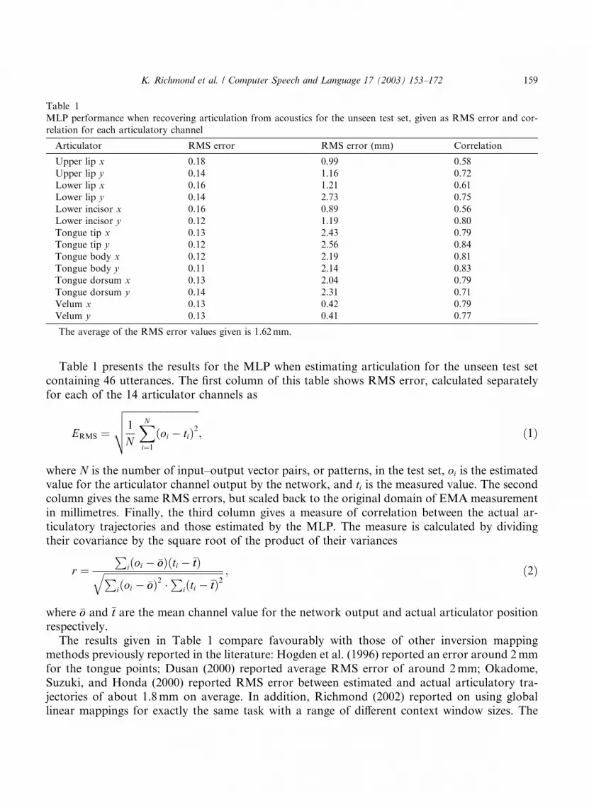
Table 1 presents the results for the MLP when estimating articulation for the unseen test setcontaining 46 utterances. The first column of this table shows RMS error, calculated separatelyfor each of the 14 articulator channels as

ERMS ¼

ffiffiffiffiffiffiffiffiffiffiffiffiffiffiffiffiffiffiffiffiffiffiffiffiffiffiffiffiffiffi1

N

XNi¼1

ðoi � tiÞ2vuut ; ð1Þ

where N is the number of input–output vector pairs, or patterns, in the test set, oi is the estimatedvalue for the articulator channel output by the network, and ti is the measured value. The secondcolumn gives the same RMS errors, but scaled back to the original domain of EMA measurementin millimetres. Finally, the third column gives a measure of correlation between the actual ar-ticulatory trajectories and those estimated by the MLP. The measure is calculated by dividingtheir covariance by the square root of the product of their variances

r ¼P

iðoi � �ooÞðti � �ttÞffiffiffiffiffiffiffiffiffiffiffiffiffiffiffiffiffiffiffiffiffiffiffiffiffiffiffiffiffiffiffiffiffiffiffiffiffiffiffiffiffiffiffiffiffiffiffiffiffiPiðoi � �ooÞ2 �

Piðti � �ttÞ2

q ; ð2Þ

where �oo and �tt are the mean channel value for the network output and actual articulator positionrespectively.

The results given in Table 1 compare favourably with those of other inversion mappingmethods previously reported in the literature: Hogden et al. (1996) reported an error around 2mmfor the tongue points; Dusan (2000) reported average RMS error of around 2mm; Okadome,Suzuki, and Honda (2000) reported RMS error between estimated and actual articulatory tra-jectories of about 1.8mm on average. In addition, Richmond (2002) reported on using globallinear mappings for exactly the same task with a range of different context window sizes. The

Table 1

MLP performance when recovering articulation from acoustics for the unseen test set, given as RMS error and cor-

relation for each articulatory channel

Articulator RMS error RMS error (mm) Correlation

Upper lip x 0.18 0.99 0.58

Upper lip y 0.14 1.16 0.72

Lower lip x 0.16 1.21 0.61

Lower lip y 0.14 2.73 0.75

Lower incisor x 0.16 0.89 0.56

Lower incisor y 0.12 1.19 0.80

Tongue tip x 0.13 2.43 0.79

Tongue tip y 0.12 2.56 0.84

Tongue body x 0.12 2.19 0.81

Tongue body y 0.11 2.14 0.83

Tongue dorsum x 0.13 2.04 0.79

Tongue dorsum y 0.14 2.31 0.71

Velum x 0.13 0.42 0.79

Velum y 0.13 0.41 0.77

The average of the RMS error values given is 1.62mm.


linear mapping with 20 frames within the context window performed with an error of 1.89mm onaverage.

RMS error and correlation scores provide a means to compare objectively and quantitativelythe performance of two different networks, or indeed different inversion techniques describedpreviously in the literature. Meanwhile, visual comparison of MLP output with the measuredarticulatory trajectories undoubtedly gives a very useful qualitative impression of how the MLP isperforming the inversion mapping, and can reveal clues as to the nature of error in the MLPoutput.

Fig. 2 demonstrates the output of the MLP for the test set utterance ‘‘The speech symposiummight begin on Monday’’. The figure provides a direct comparison of the trajectories estimatedby the MLP with those measured by EMA and normalised. Silence at the beginning and end ofthe files has been omitted. As this example shows, the MLP is typically capable of estimatingthe trajectories of some articulators with a good level of accuracy at some times, but less so atother times. For example, at around 1.8 s, the MLP estimates for the x-coordinates of the threetongue points are more accurate than for the y-coordinates of the same points. During the restof the utterance, however, the accuracy of the tongue point y-coordinate estimates is reasonablyhigh.

The inertia of speech articulators means they are constrained to move relatively slowly andsmoothly. While continuity is a basic principle of human speech production, an MLP trained withthe sum-of-squares error function will not necessarily emulate this. The aim of training with thesum-of-squares error function is to minimise the distance of the MLP output from the targetoutput for each input–output training pattern. In other words, the optimal instantaneous map-ping that the MLP can provide at a given time frame is the conditional average of the articulatorconfigurations for all such input vector frames. However, this optimum does not in any waystipulate that the output articulatory configuration at one time frame should depend on the ar-ticulatory configuration at any previous or following time frames. Therefore, we rely heavily onthe inversion mapping function itself to yield smoothly varying output. Specifically, we assumethat acoustic input vectors at time t � 1 and time t þ 1 will map to points in the near vicinity of thearticulatory configuration at time t, such that no discontinuities result in the overall sequence ofMLP output. This assumption is reasonable, but is in practice liable to be confounded by one-to-many mappings from the acoustic to the articulatory domain. For instance, the MLP outputshown in Fig. 2 appears to be noisier than the respective measured articulatory trajectories. This isdespite the use of a context window, which should help alleviate the problem of one-to-manymappings.

In an effort to make up for inadequacies in the MLP estimated articulatory trajectories, wemight turn to various postprocessing techniques. For example, we know that the articulatorsmove relatively slowly. Therefore, one simple example of an articulatory constraint we couldimpose as a postprocessing step, which utilises this knowledge, is to lowpass filter the MLPoutput. In Richmond (2002), we have demonstrated that lowpass filtering the MLP estimatedtrajectories, with channel specific lowpass cutoff frequencies which had been identified em-pirically, does indeed moderately reduce RMS error and increase correlation scores. However,we will not use this method here. In the present paper, we want simply to evaluate whether amore sophisticated description of the target articulatory domain might provide a bettermodel.


4. MDN inversion mapping

To recapitulate, the MDN provides a principled method for modelling the target data corre-sponding to each input vector with a full conditional probability density function. This contrastswith the least-squares trained MLP, which only provides a mean value and a fixed residual

Fig. 2. A comparison of the MLP estimated articulatory trajectories with the EMA-measured articulatory trajectories

for the unseen test utterance ‘‘The speech symposium might begin on Monday’’. Note the articulatory trajectories in

this plot are shown in their normalised range, after processing as described in Section 2.2.


variance for the distribution of possible target values. Moreover, the MLP assumes distributionsof target points corresponding to a unimodal Gaussian.

Since MDNs are not commonplace in the speech field, for the reader�s convenience we shall firstbriefly introduce the theory underpinning the model. For a complete description, the reader isdirected to Bishop (1994) or Bishop (1995).

4.1. Introduction to the mixture density network

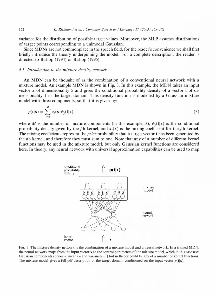
An MDN can be thought of as the combination of a conventional neural network with amixture model. An example MDN is shown in Fig. 3. In this example, the MDN takes an inputvector x of dimensionality 5 and gives the conditional probability density of a vector t of di-mensionality 1 in the target domain. This density function is modelled by a Gaussian mixturemodel with three components, so that it is given by:

pðtjxÞ ¼XMj¼1

ajðxÞ/jðtjxÞ; ð3Þ

where M is the number of mixture components (in this example, 3), /jðtjxÞ is the conditionalprobability density given by the jth kernel, and ajðxÞ is the mixing coefficient for the jth kernel.The mixing coefficients represent the prior probability that a target vector t has been generated bythe jth kernel, and therefore they must sum to one. Note that any of a number of different kernelfunctions may be used in the mixture model, but only Gaussian kernel functions are consideredhere. In theory, any neural network with universal approximation capabilities can be used to map

Fig. 3. The mixture density network is the combination of a mixture model and a neural network. In a trained MDN,

the neural network maps from the input vector x to the control parameters of the mixture model, which in this case uses

Gaussian components (priors a, means l and variances r2) but in theory could be any of a number of kernel functions.

The mixture model gives a full pdf description of the target domain conditioned on the input vector pðtjxÞ.


from the input vector to the mixture model parameters. In this example, we see a feedforwardMLP with 5 input units, a hidden layer of 2 units with sigmoidal activation and nine linear outputunits for the mixture parameters. In general, the total number of network outputs is given byðcþ 2Þ M , where c is the dimensionality of the target domain, and M is the number of mixturecomponents. In other words, each mixture component has 1 unit for its prior, 1 unit for itsvariance and c units for the mean of the component in the target space. Note that we are usingGaussian components with spherical covariance here (one variance parameter for each compo-nent). In principle, the MDN is not limited to using only spherical covariance; both a diagonal orfull covariance matrix could be used for each component. However, complicating the model inthis way is avoidable, because a mixture of spherical Gaussians is theoretically able to model anydistribution function with arbitrary accuracy assuming enough components are available (Bishop,1995).

In order to constrain the mixing coefficients to lie within the range 06 ajðxÞ6 1 and to sum tounity, the softmax function (Bridle, 1990) is used to relate the mixing coefficients of the mixturemodel to the output of the corresponding units in the neural network:

aj ¼expðzaj ÞPMl¼1 expðzal Þ

; ð4Þ

where zaj is the output of the neural network corresponding to the mixture coefficient for the jthmixture component. The variance parameters of the mixture model are related to the corre-sponding outputs of the neural network according to the following function:

rj ¼ expðzrj Þ; ð5Þ

where zrj is the output of the neural network corresponding to the variance for the jth mixturecomponent. This has the convenience of avoiding the variance becoming less than or equal tozero. Finally, the means for the mixture model are represented directly by the correspondingoutputs of the neural network:

ljk ¼ zljk; ð6Þ

where zljk is the value of the output unit corresponding to the kth dimension of the mean vector forthe jth mixture component.

The objective of training the MDN is to minimise the negative log likelihood of the observedtarget data points given the mixture model parameters, which is given by

E ¼ �Xn

lnXMj¼1

ajðxnÞ/jðtnjxnÞ( )

: ð7Þ

Since it is the neural network part of the MDN that provides the parameters for the mixturemodel for each input–output vector training pair, this error function must be minimised withrespect to the network weights. Fortunately, the derivatives of the error at the network outputunits corresponding separately to the priors, means and variances of the mixture model may becalculated (see Bishop, 1995). These error �signals� may then be propagated back through thenetwork as normal in network training to find the derivatives of the error with respect to thenetwork weights. Thus, training is a problem to which standard non-linear optimisation algo-rithms can be applied.


4.2. Application to inversion mapping task

Using a single Gaussian in the mixture model is similar to the unimodal regression observedwhen using an MLP to estimate articulation from acoustics. However, in the case of the MDN,the variance of the Gaussian as well as the mean is allowed to vary as a function of the acousticinput vector, which yields greater modelling flexibility. Using a mixture of Gaussians in theMDN pdf (see Eq. (3)) introduces the additional flexibility of allowing potentially non-Gaussian and multimodal distributions in the target articulatory domain to be modelled moreclosely.

In Richmond (2002), we compared the performance of MDNs trained for each articulatorychannel containing four combinations of either 5 or 10 hidden units and either one or twoGaussian kernels in the density model. In 27 out of 28 cases where networks were directlycompared, the MDN with a mixture of two Gaussians in the density model demonstrated higheraccuracy than the equivalent MDN with a single Gaussian. The dependence on the number ofhidden units was also indicated by a pairwise comparison of otherwise equivalent networks. In27 1 out of 28 direct comparisons, the MDN containing 10 hidden units performed better than theequivalent MDN with just 5 hidden units. For the sake of brevity, we will concentrate here on theresults for the MDNs containing 10 hidden units and 2 Gaussians in the density function for eacharticulatory channel.

This limited set of combinations of hidden layer size and density function may not include theoptimal MDN architecture. However, our aim in the current paper is simply to ascertain whetherhaving variance parameters dependent on the input on one hand and allowing multimodal dis-tributions on the other can provide a closer model of the distribution of possible target articu-latory configurations. Since our results will indicate this is the case, this limited set is sufficient forour purposes here. Nevertheless, there are strong indications that it may prove beneficial in futurework to try MDNs with higher numbers of hidden units and mixture components in order to gainbetter performance.

Exactly the same training, validation and testing data sets as were used with the MLPdescribed in Section 3 were used for training the MDNs. Thus, the MDNs in this section had400 acoustic input units, which made up the context window of 20 frames of 20 filterbankcoefficients.

Prior to training, the biases for the output units of the MDN were initialised using a k-means based initialisation algorithm. Under this algorithm, a separate Gaussian mixturemodel of the same form as the MDN output was used to model the unconditional densityof the target data. Ten iterations of the k-means algorithm were used to determine thecomponent centres. The priors were computed from the proportion of the target data be-longing to each component, and the variances were calculated as the sample variance of thetarget data points belonging to each component from the associated mean. The output unitbiases were then set so that the net would output the values in the Gaussian mixturemodel. All other biases and weights in the MDN were randomised by sampling from aGaussian.

1 Not the same 27 networks from the previous comparison between one and two Gaussian kernels.


As with the MLP, the MDNs were trained using the Scaled Conjugate Gradient algorithm tooptimise the error function given in Eq. (7). Although the separate validation set was used toidentify the best network during training, an upper bound of 2000 training epochs was also im-posed. However, all 14 networks appeared to reach a maximum in terms of performance on thevalidation set within this limit.

4.3. Results

Figs. 4 and 5 provide a visual representation of the output of the MDNs. These plots, whichmight be termed articulatory ‘‘probabilitygrams’’, show the probability density for the location ofan articulator within its range of movement as a function of time. Such plots are produced bytaking the probability density function output by the MDN at each time frame (x-axis) andcalculating the probability density at certain intervals (in this case 0.01) encompassing the range ofmovement of the given variable (y-axis). The probability density for a particular articulator lo-cation at a given time frame is represented by the greyscale intensity. Intense black indicates highprobability density, whereas white indicates low probability density.

As well as showing the output of the MDNs, the measured EMA trajectories are shown forcomparison. Phonetic segmentation is also indicated in these plots. This labelling is provided asstandard as part of the MOCHA database, and was produced automatically using the recordingprompts and an HMM forced alignment.

4.3.1. Variability of varianceIn Figs. 4 and 5, it is clear that the variance around the estimated location of an articulator is

higher at some times than at others. We also notice a correlation: when the MDN output varianceis low, the accuracy of the estimated location of the articulator is typically higher. This correlation

Fig. 4. Comparison of MDN output with the actual, measured articulator trajectory for the unseen test utterance

‘‘Bright sunshine shimmers on the ocean’’. The y-coordinate trajectory of the lower incisor is shown in this example.

Probability density over the range of the articulator�s movement is shown as a function of time using greyscale intensity,

where intense black indicates high probability density.


is unsurprising, since the variances of the probability density functions output by the MDN areestimated as a function of the acoustic input so as to minimise the negative log likelihood errorfunction.

Generally, it seems that the variance is low when the articulators might be critical to theproduction of the segment. For example, for the tongue tip articulator in Fig. 5, the varianceis lowest during times when the tongue tip is near the upper surface of the vocal tract and‘‘critical’’, such as during the phones [t, s, z]. Table 2 explores this observation in greaterdepth.

For each of the three articulatory channels in Table 2, we have calculated the average varianceoutput by the respective MDN during all frames in the test set corresponding to 23 separatephones. 2 Channel specific MDNs containing 10 units in a single hidden layer and a singleGaussian kernel in the output pdf were used for this purpose (Richmond, 2002). For each ar-ticulatory channel, we have then ranked the phones according to their respective MDN averagevariance.

On the whole, the results in Table 2 are consistent with our initial observation. For ex-ample, we find that for the ‘‘tongue tip y’’ channel, those phones for which the position of thetongue tip is critical demonstrate lower average variance, such as [s, z, h. . .]. Meanwhile, forthe ‘‘upper lip x’’ channel, phones such as [m, w, b, p] demonstrate lower average variancerelative to other phones. In the third column, for the ‘‘velum x’’ channel, it is interesting tonote that the MDN output features lower average variance for those phones where the velarport is most likely to be closed, whereas for the nasal stops [m, n, ¢] the average variance isrelatively high.

2 The remaining 23 phones in the phone set that have not been included in Table 2 were all vowels.

Fig. 5. Comparison of MDN output with the actual, measured articulator trajectory for the unseen test set utterance

‘‘Most young rabbits rise early every morning’’. The y-coordinate trajectory of the tongue tip is shown in this example.

Probability density over the range of the articulator�s movement is shown as a function of time using greyscale intensity,

where intense black indicates high probability density.


There are of course certain caveats to bear in mind when considering the results in Table 2.From a practical point of view, it is possible that the picture is clouded to some extent by the useof the automatically produced MOCHA labelling, which in some respects is closer to a ‘‘pho-nological’’ labelling rather than a fine-grained ‘‘phonetic’’ labelling: for example, any instances ofglottal stops will be labelled as the underlying phone; instances of assimilation are overlooked; nodistinction is made between dark and light [l], and so on. In other words, the phone classes usedmay not correspond to satisfactorily pure groups of allophones. It is also possible, hypotheticallyspeaking, that an articulator�s position may not be critical to the production of a given phone, butthat its position may nevertheless be relatively accurately predicted (perhaps under the influenceof a critical articulator). Finally, when interpreting these results, it is important not to forget thatthe variances in question are not those exhibited directly by the articulators themselves. Instead,they are the variance parameters from the MDN output pdfs, which are only an approximation tothe conditional probability density of the real data. However, despite these caveats, we never-theless believe these findings tend to support the view of critical versus non-critical articulatorsdiscussed by Papcun et al. (1992).

Table 2

Ranked phone dependent averages for the variance parameters of MDN output density functions for three articulatory

channels

Tongue tip y Upper lip x Velum x

Phone Av. r2 Phone Av. r2 Phone Av. r2

s 0.003 m 0.015 T 0.007

z 0.003 w 0.016 z 0.007

h 0.005 D 0.017 b 0.008

S 0.006 n 0.018 S 0.008

t 0.009 b 0.019 s 0.008

D 0.010 p 0.019 g 0.009

T 0.011 N 0.019 F 0.009

n 0.011 k 0.020 t 0.009

y 0.012 f 0.020 y 0.009

N 0.012

r

0.020 d 0.010

d 0.012 g 0.020 k 0.011

r

0.012 l 0.021 f 0.011

F 0.013 v 0.021 h 0.011

v 0.013 h 0.021 w 0.012

f 0.013 d 0.021 p 0.012

l 0.014 h 0.021 v 0.012

m 0.014 z 0.022 l 0.013

h 0.014 t 0.024 D 0.013

g 0.014 s 0.027

r

0.018

k 0.015 F 0.027 N 0.021

w 0.016 T 0.028 m 0.024

p 0.017 S 0.028 h 0.025

b 0.017 y 0.029 n 0.037

Phone identities are given using standard IPA notation. Notice that the MDN output generally features lower

variance where an articulator�s position could be considered to exert a strong influence during the production of a

phone.


4.4. MDN output flexibility

The probability density function over the target domain which the MDN provides is a flexiblemodel in itself and may be used in numerous ways according to requirement. For example, wecould compute the conditional mean of the target data given the input vector. This value ap-proximates the output of a standard least-squares trained MLP as a special case. We could alsocompute the variance around this average for each input vector. This goes beyond the capabilitiesof a standard MLP, for which we can only compute a global residual variance. On the other hand,at each time frame, we could take the mean and variance of the Gaussian with the highest prior togive the mode trajectory. This approximates the mixture of experts model (Jordan & Jacobs, 1994)as another special case. While these few examples give an impression of the flexibility of the MDNoutput, many other ways of using the MDN output may be envisaged.

5. Comparing MLP with MDN

In order to gauge whether MDNs allow closer modelling of the distributions of possible ar-ticulatory configurations than MLPs, we require an error measure to compare like with like. If weassume that the MLP has sufficient representational power and has been trained well enough toapproximate closely the conditional mean of the target data, we know that any remaining error isattributable to the variance of the target data itself around its conditional mean (Bishop, 1995).

The global variance for each articulatory channel (r2k) may be calculated as

r2k ¼

1

N

XNn¼1

ykðxn;w�Þ

� tnk�2; ð8Þ

where N is the number of input–output vector pairs in the training set, ykðxn;w�Þ is the kth outputof the trained MLP with the optimal weight configuration w� in response to the acoustic inputvector xn, and tnk is the corresponding articulatory target value for channel k.

Hence, at testing time, we can interpret the MLP output for each time frame as a singleGaussian probability density function, whose mean and variance are given respectively by theoutput of the MLP and the global variance precomputed according to Eq. (8). Given theprobability density functions at each time frame, we can calculate the likelihood of the articu-latory target data for the whole test set. This likelihood can be compared directly with theequivalent likelihood calculated according to the probability density functions provided by theMDNs.

Table 3 provides just this comparison. Columns 2 and 3 of Table 3 give the geometric meanlikelihood of the articulatory target data in the test set, 3 given the framewise probability densityfunctions computed from the MLP and MDN, respectively. This was calculated by dividing thetotal log likelihood by the number of input–output pairs in the test set, then transferring back outof the log domain. In column 4 we have calculated the relative improvement of the MDN modelover the MLP in terms of these likelihoods as a percentage.

3 There were 11, 660 acoustic-articulatory feature vector pairs in the test set.


To reiterate Section 1.2, in performing this comparison, we are effectively asking whether there isany point in attempting to model the distribution of possible articulatory points conditioned on theinput vector, andwhether using distributionsmore complex than a singleGaussian can also providea better model. If the residual error in the MLP inversion mapping were due to machine measure-ment error, or any other source of error thatwas not dependent on the acoustic signal, thenwewouldnot expect to see any benefit in using the MDN. However, if the distribution of target articulatorypoints does depend to any extent on the acoustic input, and thus is characteristic of the inversionmapping function itself, then the MDN should demonstrate a higher likelihood score.

As the last column of Table 3 makes clear, the use of MDNs does indeed yield higher likelihoodscores for all articulatory channels. The size of this improvement ranges from 2.6% to 21.8%.Apart from for the velum, it would appear that the best improvement is observed for the y-co-ordinates of the articulators. Excluding the velum channels, the average improvement for thearticulatory-coordinates is about 13.3%, whereas the average for the x-coordinates is only 4.8%.In future work, it would be interesting to investigate what might be the reason for this disparity.For example, it may be this is merely coincidence, or an idiosyncrasy of this particular speaker.On the other hand, it could be a more general observation. Experiments using data from multiplespeakers would be useful to investigate this question.

5.1. Density function form

As mentioned in Section 4.2, we have found that MDNs with 2 Gaussian kernels outperformedMDNs with a single Gaussian on the same inversion mapping task in 27 out of 28 cases ofcomparison. This indicates that the reason the MDNs outperform the MLP in Table 3 is at leastin part due to greater flexibility for modelling non-Gaussian distributions.

Table 3

A comparison of the likelihood of the test set target data given the framewise probability density functions provided by

MLP and MDN

Articulator channel MLP mean likelihood MDN mean likelihood Increase %

Upper lip x 1.35 1.40 4.4

Upper lip y 1.69 1.83 8.2

Lower lip x 1.52 1.56 2.6

Lower lip y 1.75 1.88 7.4

Lower incisor x 1.49 1.57 5.3

Lower incisor y 2.04 2.48 21.8

Tongue tip x 1.90 2.01 5.4

Tongue tip y 2.11 2.56 21.4

Tongue body x 1.97 2.08 5.4

Tongue body y 2.18 2.38 9.0

Tongue dorsum x 1.92 2.02 5.6

Tongue dorsum y 1.79 2.00 11.9

Velum x 1.90 2.14 12.7

Velum y 1.88 2.00 6.7

Here, 14 channel specific MDNs have been used with 10 units in one hidden layer and an output mixture density

model comprising two Gaussian kernels. The likelihood figures for both MLP and MDN are given as the geometric

mean, calculated over all input–output pairs in the unseen test set.


Fig. 6 illustrates this point. This figure shows the density function output by the MDN for they-coordinate of the tongue tip at frame 255 of utterance fsew0_026 (as shown in Fig. 5). Thisconditional density function is clearly different from a unimodal Gaussian. We have also markedthe actual articulator location on this plot with an ‘‘x’’, and overlaid a unimodal Gaussian whosemean is given by the MLP output and whose variance is the residual variance calculated accordingto Eq. (8). If we assume the probability density function provided by the MDN is a reasonableapproximation to the real conditional distribution of the target data, we see that by accommo-dating the probability mass under the ‘‘lobe’’ on the right hand side (apparently centred just below0.7), the accuracy of the MLP estimate of the articulator position has been compromised.

6. Conclusion

A feedforward MLP has been presented and applied to the task of recovering articulatorytrajectories from acoustics during continuous, phonetically rich speech. This network was trainedand tested using measured articulatory-acoustic data.

While the performance of this network compared favourably with the results of other inversionmethods reported in the field, we suspected that the MLP was ill-suited to estimating articulationfrom acoustics in at least two respects. First, the MLP is limited to modelling target data points

Fig. 6. The probability density function output by the MDN (containing 10 hidden units and a mixure density model of

two Gaussian components) for the y-coordinate of the tongue tip at frame 255 (/¢/ phone) of utterance fsew0_026 (as

shown in Fig. 5). The conditional density function output by the MDN at this point is clearly not consistent with a

unimodel Gaussian. For comparison, we also include the equivalent density function for the MLP output, as well as the

y-coordinate of the tongue provided by EMA.


with a unimodal Gaussian, which is not necessarily a sound assumption to make when modellingthe inversion mapping. Second, the MLP gives no indication of the variance of the distribution ofthe target points around the conditional average.

In theory, the MDN is able to provide a description or model of the target domain at each timeframe which is powerful enough to overcome these shortfalls. In order to verify this, we havesought to compare directly the performance of the MDN with that of the MLP on the sameinversion task.

By reinterpreting the MLP output error in terms of the likelihood of the target data, we havedemonstrated that the MDN does indeed provide a more accurate model of the distribution of thetarget variables in the articulatory domain with respect to the inversion mapping problem. Thisresult is relevant not only to those using MLPs in particular to perform the inversion mapping,but wherever similar assumptions about the conditional distribution of articulatory parametersare made.

Furthermore, we have indicated evidence that might explain how this improvement is realised.Specifically, we have shown that the MDN is able to accommodate the fact that the positions ofthe articulators may be more constrained, and thus more reliably estimated, at some times than atothers. In addition, the MDN is better able to handle cases where the conditional distribution ofarticulator positions does not correspond in form to a unimodal Gaussian, for example where thesolution to the inversion mapping has multiple branches.

7. Future work

This paper has concentrated on demonstrating that the MDN is able to provide a more flexibleand accurate model of the articulatory domain when attempting to infer articulatory parametersfrom the acoustic speech signal. However, we have not considered how the output of an MDNmight best be used in applications. Although we touched briefly on a few values that might becomputed from the pdf output by the MDN in Section 4.4, we have by no means exhausted thescope of possibilities.

Future work will therefore focus specifically on exploring how best to exploit the MDN output.The aim will be to derive the ‘‘best-guess’’ trajectory through the sequence of density functions.For example, one method envisaged would be to use Kalman smoothing, where the varianceoutput by the MDN is used as an estimate of the measurement error of the articulator positionobservations. Articulatory constraints of varying degrees of complexity could be employed withinthis technique. Perhaps the simplest would be to constrain the articulators to move slowly fromone time frame to the next. More sophisticated articulatory constraints could be instantiated byfollowing the approach of Dusan (2000), who used trained Kalman filter parameters specific tothe transition between all phones in the phone inventory.

Acknowledgements

The authors would like to thank Steve Isard for contributing many valuable comments andsuggestions in response to previous drafts, and Alan Wrench for help with the MOCHA data.


References

Atal, B.S., Chang, J.J., Mathews, M.V., Tukey, J.W., 1978. Inversion of articulatory-to-acoustic transformation in the

vocal tract by a computer sorting technique. J. Acoust. Soc. Am. 63, 1535–1555.

Bishop, C., 1994. Mixture density networks. Technical Report NCRG/4288, Neural Computing Research Group,

Department of Computer Science, Aston University, Birmingham, B4 7ET, UK, February.

Bishop, C., 1995. In: Neural Networks for Pattern Recognition. Oxford University Press, Oxford.

Bridle, J.S., 1990. Probabilistic interpretation of feedforward classification network outputs, with relationships to

statistical pattern recognition. In: Neurocomputing: Algorithms, Architectures and Applications. Springer, Berlin,

pp. 227–236.

Dusan, S., 2000. Statistical estimation of articulatory trajectories from the speech signal using dynamical and

phonological constraints. Ph.D. Thesis, Department of Electrical and Computer Engineering, University of

Waterloo, Waterloo, Canada, April.

Hogden, J., Lofqvist, A., Gracco, V., Zlokarnik, I., Rubin, P., Saltzman, E., 1996. Accurate recovery of articulator

positions from acoustics: new conclusions based on human data. J. Acoust. Soc. Am. 100 (3), 1819–1834.

Jordan, M., Jacobs, R., 1994. Hierarchical mixtures of experts and the EM algorithm. Neural Comput. 6 (2), 181–214.

Lindblom, B., Lubker, J., Gay, T., 1979. Formant frequencies of some fixed-mandible vowels and a model of speech

motor programming by predictive simulation. J. Phonet. 7, 147–161.

Mermelstein, P., 1973. Articulatory model for the study of speech production. J. Acoust. Soc. Am. 53 (4), 1070–1082.

Møller, M., 1993. A scaled conjugate gradient algorithm for fast supervised learning. Neural Networks 6 (4), 525–533.

Mozer, M.C., Smolensky, P., 1989. Skeletonization: a technique for trimming the fat from a network via relevance

assessment. In: Touretzky, D.S. (Ed.), Advances in Neural Information Processing Systems, vol. 1. Morgan

Kaufmann, Los Altos, CA, pp. 107–115.

Okadome, T., Suzuki, S., Honda, M., 2000. Recovery of articulatory movements from acoustics with phonemic

information. In: Proc. 5th Seminar on Speech Production. Kloster Seeon, Bavaria, pp. 229–232.

Papcun, G., Hochberg, J., Thomas, T.R., Laroche, F., Zachs, J., Levy, S., 1992. Inferring articulation and recognising

gestures from acoustics with a neural network trained on X-ray microbeam data. J. Acoust. Soc. Am. 92 (2), 688–

700.

Rahim, M., Goodyear, C., Kleijn, W., Schroeter, J., Sondhi, M., 1993. On the use of neural networks in articulatory

speech synthesis. J. Acoust. Soc. Am. 93 (2), 1109–1121.

Rahim, M.G., Kleijn, W.B., Schroeter, J., Goodyear, C.C., 1991. Acoustic-to-articulatory parameter mapping using an

assembly of neural networks. In: Proceedings of the IEEE International Conference on Acoustics, Speech, and

Signal Processing, pp. 485–488.

Richmond, K., 2002. Estimating articulatory parameters from the acoustic speech signal. Ph.D. Thesis, The Centre for

Speech Technology Research, Edinburgh University.

Roweis, S., 1999. Data driven production models for speech processing. Ph.D. Thesis, California Institute of

Technology, Pasadena, California.

Shirai, K., Kobayashi, T., 1986. Estimating articulatory motion from speech wave. Speech Commun. 5, 159–170.

Wakita, H., 1979. Estimation of vocal-tract shapes from acoustical analysis of the speech wave: the state of the art.

IEEE Trans. Acoust. Speech Signal Process. ASSP-27, 281–285.

Westbury, J.R., 1994. X-ray microbeam speech production database user�s handbook. Technical Report Version 1.0,

University of Wisconsin, Madison.

Wrench, A., Hardcastle, W.J., 2000. A multichannel articulatory speech database and its application for automatic

speech recognition. In: Proc. 5th Seminar on Speech Production. Kloster Seeon, Bavaria, pp. 305–308.

Zachs, J., Thomas, T.R., 1994. A new neural network for articulatory speech recognition and its application to vowel

identification. Computer Speech Language 8, 189–209.


modelling the uncertainty in recovering articulation from acoustics

Documents