Assessing the sound of a woodwind

instrument that cannot be

played

D. Keith Bowen a,⇑, Kurijn Buys b, Mathew Dart c , David Sharp b

a Royal College of Music, Prince Consort Road, London SW7 2BS, UKb The Open University, Milton Keynes, UKc London Metropolitan University, London, UK

a r t i c l e

i n f o

Article history:

Received 30 May 2018Received in revised form 20 August 2018Accepted 28 August 2018

a b s t r a c t

Historical woodwind instruments in museums

or private collections often cannot be played, by virtue oftheir poor condition or the risk of damage.

Acoustic impedance measurements

may usually be performedon instruments in good condition without risk of damage, but only if they are in playable condition: com-plete, with functioning mechanism, well-sealing pads and no open cracks. Many museum specimens arenot in this

condition. However, their geometry may almost always be

accurately measured, and

the mea-surements used to calculate the acoustic impedance as a function of frequency via a computer model ofthe body of the instrument. Conclusions may then be drawn about the instrument’s pitch, intonation,temperament, fingerings, effects of bore shrinkage and even the timbre of the notes. A simple linear,plane- and spherical-wave computational

model, originally developed for calculating the acoustic impe-dance of conical-bore woodwinds, is here applied to

bass clarinets

for the first time. The results areassessed by experimental impedance measurements and by playing

tests on an historical Heckel bassclarinet in A of 1910 that has been continuously maintained in playing condition but has been relativelylightly used. The degree of agreement between the acoustic measure ments and the calculations, therequired measurement accuracy

and the potential and limitations of

the method are discussed, and speci-fic conclusion s for this instrument are drawn. Measurement of the frequencies produced in playing testsallowed us quantitatively to estimate the effects of mouthpiece and reed on the pitch of the producednotes. The method is shown

to be a viable method for the examination of historical woodwindinstruments.

Ó

2018 Elsevier Ltd. All rights reserved.

1. Introduction

The aim of

the investigations

in this paper is to test the idea thatit

is possible to model the input impedance of a woodwind instru-ment sufficiently accurately that one may

draw reliable conclu-sions about its behaviour purely from geometrical measurementsof its bore, tone holes and keypads. This will enable the vast collec-tions of woodwind instruments in museums to

be used for primaryevidence of their sounds without risk of damage.

There is a very large number of musical instruments in museumcollections

in the UK alone.

These are steadily being catalogued inthe MiniM database, which contains 20,000 records so far .[1]Clearly, a very important property of a musical instrument is itssound and related questions such as its pitch, temperament andfingering. However, the overall responsibility of museums is toprotect and promote the tangible and intangible natural and cul-tural heritage , and

many institutions preclude playing the[2]instruments because of

the risk of damage . This is especially[3]

true for woodwind instruments where the act of

playing rapidlyintroduces air at a much higher humidity and temperature, trigger-ing potentially damaging reactions

in the

wood. Moreover, even ifplaying is permitted, it is fairly unlikely that a wind instrument150–200 years old will be usefully

playable without

restorationthat goes well beyond normal conservation.

Sealing against leaksis crucial in these instruments; 200-year old pads – when original– are likely to leak, and cracks in the wooden body are quite

fre-quent. These leaks strongly affect the acoustic impedance, render-ing the instrument useless for the assessment of its musicalpotential either by playing or by acoustic impedance measure-ment. Occasionally

a museum will permit full restoration for play-ing on a special occasion. Examples are the Brussels Musée desInstruments de Musique, where an Adolphe Sax instrument (B.B.mim.2601) was partially overhauled to play in the Sax bicentenarycelebrations in 2014, and the Robert Schumann School in Düssel-dorf, where a Stengel bass clarinet in A, originally owned by theBayreuth Theatre and used in some original Wagner operatic per-formances, was restored for a demonstration concert and futureuse . But the great majority of wind instruments in museums[4]

https://doi.org/10.1016/j.apacoust.2018.08.0280003-682X/ 2018 Elsevier Ltd. All rights reserved.Ó

⇑ Corresponding author.

E-mail address: keith.bowen@rcm.ac.uk (D.K. Bowen).

Applied Acoustics 143 (2019) 84–99

Contents lists

available at ScienceDirect

Applied Acoustics

j o u r n a l

h o m e p a g e :

w w w . e l s e v i e r . c o m / l o c a t e / a p a c o u s t

remain musically hidden from players or from direct sampling ofthe sound.

However, museums will normally permit the

handling andcareful measurement of instruments that are not too fragile, byan accredited researcher under supervision and the guidelines

ofICOM/CIMCIM . This has been used to study the development[5]of types of musical instrument and their keywork (see,

for exam-ple, for clarinets),

but their sounds have so far been mostly[ ]6–8inaccessible.

The

principle upon which the main methodology of this

paper isbased is

that the sound of a wind instrument

is dominated by theshape of its air column, as indicated by its input impedance.Although there are (and probably always have been) endless

argu-ments about the influence of materials on a wind instrument, it hasbeen demonstrated that the energy radiated by the walls of thetube into the room is inaudible

in

comparison with that emittedby vibration of the air column, and that wall material has littleaudible effect, as long

as it is

reasonably dense and has low poros-ity . There is also very clearly an acoustic cooperation[ ]9–11between the mouthpiece/reed and the resonator or air column,and the mouthpiece is of great importance for the details

of thetimbre and for the ease of playing. However, the importance ofthe resonator is shown by the observation that the character ofthe instrument appears mostly to go with this rather than withthe mouthpiece : a clarinet-type mouthpiece of suitably small[12]volume works reasonably well on an oboe; the instrument stillsounds like an oboe not

like a clarinet, and it overblows an octavenot a twelfth . In this paper we are concentrating on the res-[ , ]13 14onator. Its acoustic properties are defined by the sets of resonance,or

impedance, peaks that it possesses and the relationshipsbetween them. If we can understand the influence of the detailedshape of the

air column on the sound production, for all notesand all relevant frequencies, we shall know a great deal aboutthe nature of the instrument. Furthermore, this knowledge isobjective, and not subject to the physiology or prejudices of anyplayer.

A well-preserved instrument from 1910

was used to makequantitative comparisons for this trial. Standard acoustic computa-tional methods (described below) were used to calculate the impe-dance spectrum for each note of the instrument, and two tests ofthe accuracy were performed: one by measuring the input impe-dance directly in the laboratory, and the other by playing testson the instrument, measuring the frequency of the note emittedat each fingering and looking at

the predicted intonations pro-duced by both ‘normal’ and ‘alternative’ fingerings. Thus we inves-tigate two questions: can we calculate impedance spectra withsufficient accuracy without playing the instrument, and does thisgive significant musical information about the instrument?

2. Modelling of woodwind instruments

The

development of mathematical and computational methodsof modelling woodwind instruments has taken place over morethan a century, beginning with the analytical ideas of Hemholtz[15] [16]. Major contributions were made by Bouasse and byBenade and his collaborators . The understanding of

woodwind[10]acoustics progressed through analytical expressions for losslessand then

lossy systems

, linear system calculations

,[ ]17–19 [20]analysis of the reed/mouthpiece system [e.g.

, impe-[ , ]15 21–23dance of

the bell , non-linear treatment of the reed genera-[ , ]24 25tor and other factors; an excellent recent treatment appears in[26]Chaigne and

Kergomard . In 1979, Plitnik and Strong first[27] [28]

applied the computer modelling method to the whole instrument.They split the bore

(of an oboe in this case) into short cylindricalsegments, thus approximating the conical shape of the bore by

the staircase approximation, started from the calculated impe-dance of the bell

radiating into open

air and summed

each compleximpedance, in series for the

segments and in parallel for the toneholes. A reed cavity impedance was added

in parallel at the endof the sum. The result was the spectrum of impedance peaks as afunction of frequency over the audible band. Note that this andmost other approaches are based on linear theory and strictly onlyapply to small amplitudes. The non-linear effects of large ampli-tudes are critical in the understanding of the peaks selected, as dis-cussed below, but

there is agreement amongst all

authors citedthat linear acoustics suffices for the calculation of

the tuberesonances.

This general approach is still used today. Developments sincePlitnik and Strong include improvements to the expressions fortone hole impedances, for wall losses, for the radiation impedanceof the bell, for the influence of the reed generator and in the matrixformulation (analogous to electrical transmission line theory)which significantly

speeds up the calculation . Ned-[ , , ]29 34 35erveen has added valuable insight into the elements

of the[30]modelling equations and a number of experimental measure-ments. Research on simulating clarinet and

saxophone soundsdynamically using digital formulations of the air

column

and reed/mouthpiece system

in the time

domain are also reaching an inter-esting stage .[ , , , ]23 31 32 34

Two computer implementations of linear acoustic modellinghave been made more widely available and are cited in the litera-ture. The program IMPEDPS was written by Robert Cronin in the1990s, based on the developments and equations given by Keefe[29] and by discussions with Keefe and Benade. RESONANS wasdeveloped around the same time by IRCAM and the acousticsdepartment of the Université du Maine in Le Mans (a brief noteon application to recorders is given by Bolton ). Valuable sum-[33]maries of the necessary equations for each

component of the

trans-mission

line matrix

formulation have been given by Scavone [34]and more recently Yong .[35]

It turns out that the methodology descended

from Plitnik andStrong is quite general for woodwind instruments that have reedgenerator excitation. It may also be used for flutes and recordersby using admittance peaks rather than impedance peaks, sincethe open entry ends of air-driven oscillators require a pressurenode rather than antinode at the entry end. We have thereforeused the methodology to test the basic assertion, that acousticimpedance spectra can be calculated by geometric measurementson instruments to sufficient

accuracy to give musically usefulinformation. We first review the advances in understanding ofwoodwind instruments that have been made

by both experimentaland theoretical modelling of impedance spectra.

2.1.

Applications of impedance spectra to the understanding of

woodwind instruments

The understanding of the influence of impedance spectra camefirst through experimental measurements and approximate ana-lytical solutions of the acoustic equations, with

particularly nota-ble contributions made by

Benade (summarised in ), Backus[10][20,54] and their co-workers. Indeed, the increased understandingof instrument acoustics provided by measurements and calcula-tions of input

impedance led Benade directly to a new design ofclarinet bore and keyhole placement, in which inaccuracies in into-nation were

corrected by enlargement or contraction of the borearound pressure nodes . Clarinets to the ‘Benade NX design’[ ]36–39are manufactured by Stephen Fox Clarinets (Toronto) .[40]

There are various different ways in which input impedance canbe measured experimentally. Dalmont provides a compre-[ , ]41 42hensive review of input impedance measurement techniquesdeveloped during the

20th century. One of the most popular

D.K. Bowen et al. / Applied Acoustics 143 (2019) 84–99 85

approaches (pioneered by

Benade and Backus) exploits the directdefinition of impedance as the ratio between input pressure andacoustic volume flow. The approach involves passing an acousticsignal generated by a loudspeaker through a high impedancecapillary and then into the instrument under investigation. Thevolume flow entering the instrument can be determined fromthe pressure in the cavity between the loudspeaker and thecapillary. By then measuring

the pressure at the entrance to theinstrument, the input impedance can be deduced. In earlycapillary-based measurement systems, a feedback loop wasemployed to maintain

the cavity

pressure (and therefore the vol-ume flow injected into the instrument) constant, such that thepressure measured at the entrance to the instrument

was directlyproportional to the input impedance. In more modern systems, thecavity pressure is determined as a function of frequency, eitherusing a second microphone positioned within the cavity, or via cal-ibration. A very compact

and portable capillary-based system hasbeen developed by

the Institute of Musical Acoustics, Vienna; thissystem is commercially-available and is known as BIAS (BrassInstrument Analysis System). As its acronym implies, it was

origi-nally developed for brasswind, and later modified for woodwind[43] and it has been applied in the quality control of brasswindinstruments since 1989 . The knowledge and application of[44]impedance and other scientific measurements to instrument man-ufacturing has been assisted in recent years by the Pafi collabora-tion (Plateforme modulaire d’aide à la facture Instrumentale,[45]) in

France, which seeks to make scientific measurements,including input impedance, available to small

manufacturerstogether with tools to predict the effects of changes.

Another method of measuring acoustic impedance is acousticpulse reflectometry. In this method, an acoustic pulse is sent intothe instrument under test and the reflected signal is measured.Analysis of the reflected signal enables the input

impulse responseof the instrument to be determined, from which both its bore pro-file and input impedance can be calculated. Details of this methodcan be found in .[ ]46–48

Many of the studies have been made primarily to test the mod-elling theory, rather than to investigate

modern or historicalinstruments themselves. Campbell

has

written a review of theacoustic evaluation of wind instruments but the entry on wood-wind instruments is

very short . The only acoustical

investiga-[49]tions of historic clarinets appears to be the work of Jeltsch and co-workers. Jeltsch, Gibiat and Forest were able to perform acousticimpedance measurements on a set of four six-key clarinets madeby

Joseph Baumann (fl. Paris, c. 1790 – c. 1830) . The

set was[50]in

very good condition and playing was

permitted, so they couldcompare impedance measurements with

playing

frequencies, andalso make comparisons with a modern (Noblet) clarinet. The setof historical clarinets was particularly interesting, since theirmaker supplied the distinguished clarinettist and pedagogueJean-Xavier Lefévre, who refers to these clarinets in his famoustutor and gives particular fingerings to exploit or overcome[51]their characteristics. In their data analysis they concentrated onthe harmonicity relations produced by the fingerings of the clar-inets. They showed,

for example, that the first register was not welltuned, and also invented the concept of ‘impedance maps’, whichclearly show the tuning and harmonicity relationships in the Bau-mann instruments.

Lefévre remarked on the

tuning in his tutor andalso composed his sonatas mainly in the second register of theinstrument. The modern clarinet showed much better alignmentof the harmonics. We use and develop the impedance map conceptfurther in the present study ( ). Jeltsch et al. alsoSection 5.3observed that higher notes

of the instruments were supported byapparently random combinations of resonances; we shall alsoreturn to this point in . Jeltsch and Shackleton haveSection 5.3

performed

a similar study on early nineteenth century clarinetsby Alexis Bernard and Jacques Francois Simiot .[52]

The first application of computational impedance modelling toa complete instrument was by Plitnik and Strong in 1979 to[28]the oboe. Their

main concern in the modelling was to demonstratethe close agreement between calculated and measured impe-dances. This

indeed was found, with peaks being accurately locatedand

peak shapes in good agreement, though the peak-to-valleyratios in the experimental measurement were typically a factorof 2 lower than in the simulation. They ascribed this tounaccounted-for losses, in particular pad and finger resilience,socket junctions and

sharp corners of tone holes, and

we shouldexpect similar discrepancies in the case of clarinets. They investi-gated a single oboe and were able to demonstrate why certainnotes were ‘bad’ and why certain

alternative

fingerings worked.No application to historical instruments was made. Soon after,Schumacher developed the theory of

the clarinet to include[53]the reed/mouthpiece generator and used

a similar computationalapproach to Plitnik and Strong. He tested the theory on the exper-imental measurements of Backus on a single clarinet and[54]obtained similarly good agreement.

In the 1990s the IMPEDPS program was written by

Cronin andapplied to the understanding of the behaviour of fingerings andauxiliary

fingerings on modern and replica baroque bassoons[55,56]. He was able

to demonstrate the

reasons for ‘surprising’ fin-gerings shown in contemporary fingering charts for the baroquebassoon, hence

was able to obtain useful information on historicalinstruments by impedance calculations.

One of the authors of the current

paper, Dart, himself a maker ofreproduction baroque bassoons, applied computational impedancemodelling to the study of historical instruments in museums, in2011, also using IMPEDPS . He examined approximately 80%[57]of surviving baroque bassoons, making detailed internal measure-ments of thirty-six and computing impedance spectra. Thisenabled him to compare stylistic traits, to establish a new typologyof baroque bassoons and to study eighteenth-century woodwindconstruction processes and tooling. He was

also able to discoverconnections between an instrument’s internal design and its prob-able playing characteristics. In two cases of incomplete historicalinstruments, he reconstructed the design and then built replicasof each. He found

them to have different playing characteristicswhich could be understood in terms of their calculated acousticimpedance spectra.

In an investigation reported in 2012, Hichwa and Rachor [58]used similar acoustic models to Keefe in a new program designedto investigate the effects of

geometry in more detail, and

to applymathematical analysis to the results. From measurements of 44original bassoons and 14 reproductions from the baroque and earlyclassical period, they were able to deduce the temperaments usedby the original makers, which clustered in identifiable classesaround

mean-tone temperament. They showed by analysis howbest the boot joint can be made to aid intonation. They were alsoable to identify

acoustic inadequacies in some of the originaldesigns, normally in

the wing-joint, thus aiding the period-instrument maker in the selection of instruments to reproduce.

Dalmont, Gazengel,

Gilbert and Kergomard have assessed clar-inets, alto saxophones and oboes , using both impedance mea-[59]surements and the RESONANS software, and reached valuableconclusions about the quantitative influence of the reed impe-dance, the placement of the register hole, and the measurementand

effect of inharmonicity in the resonances.Sharp and co-workers have applied impedance measurement

by both the capillary system and acoustic pulse reflectometry(see ) to the question of consistency of large-scale man-Section

4.2ufacture of woodwind

instruments: trumpets , oboes and[60] [61]

86 D.K. Bowen et al. / Applied Acoustics 143 (2019)

84–99

clarinets [62]. In the case of oboes, for example,

significant playingdifferences between instruments were found to be caused by rela-tively minor variations, such as in the venting height

of one key,indicating that instrument variability can be at least partly due tothe final regulation of the instrument. However, there were also lar-ger quality-control differences such as variations in the bore profile.

3. Computational methodology

Our approach has been based largely on the equations devel-oped by Keefe , and uses his expressions for the impedance[29]of conical segments including thermal and viscous losses, and fortone holes (closed, open and open with a key pad at a certain dis-tance above the hole). Keefe’s paper includes most of the advancesmade in theoretical modelling since Plitnik and Strong and wasverified by experiments made by himself and Cronin. It is a linear,small signal plane- and spherical-wave approach. We

shall discussand cite sources for the key parameters and the necessary equa-tions. These are, the input constants, the radiation impedance ofa bell, the impedance of a conic

section (with thermal and viscouslosses at a smooth wall), the tone hole impedances (open, closedand with a pad above) and the

reed impedance.

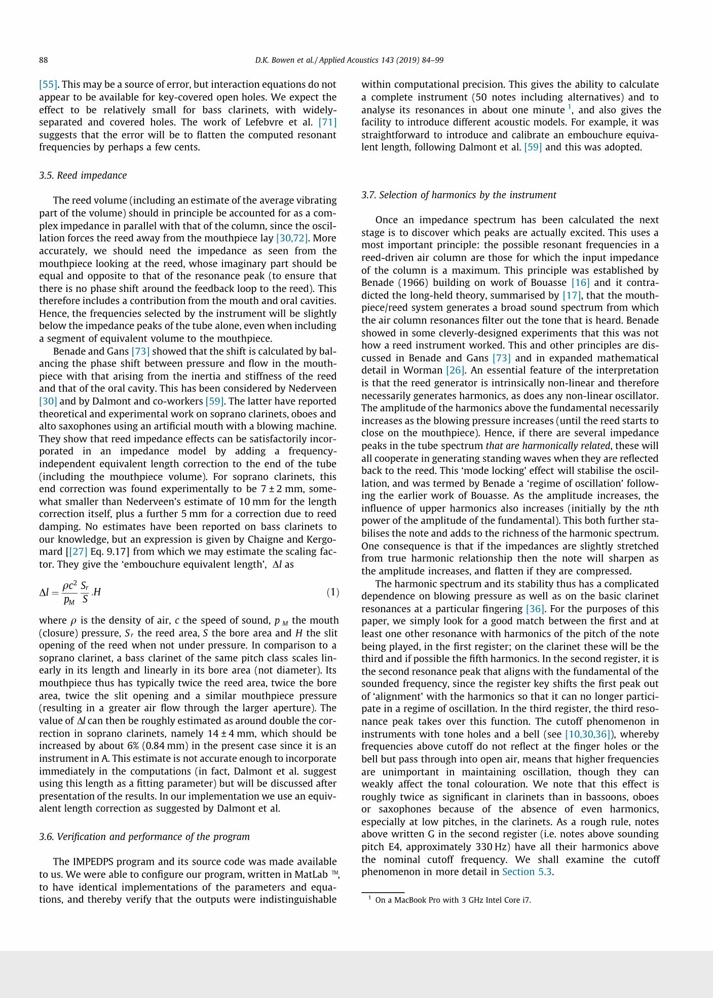
3.1. Input parameters

The

following parameters were used:

Speed of sound: 347 m s 1

Density of air 1.19 kg.m 3

Viscosity of air 1.85 10 05 Pa.sSpecific heat ratio C p/C v 1.4Thermal conductivity of air 2.63 10 02 W.m1 .K1

Specific heat at constant pressure C p 1.006 J.kg1.K1

The parameters above were chosen for appropriate playing condi-tions, that is, a somewhat elevated temperature (27 C) and humid-°

ity and a substantially elevated CO 2 content of the exhaled air .[30]The laboratory measurements were made under normal laboratoryconditions, approximately

20 C and normal atmospheric composi-°

tion. Coincidentally but conveniently, the product of air density andspeed of sound (which determines resonant frequencies) for thesetwo conditions agree to better than 1 part in 8000. This is approx-imately 0.2 cents, below the limits of audible perception, so weneed no corrections

when comparing theoretical and experimentaldata.

3.2. Radiation impedance of a bell

The

precise calculation of the radiation impedance for a ducttermination of various shape and flare is the subject of manypapers (for example, ). As noted by Chaigne and Ker-[ , , , ]24 25 27 63gomard , p. 684], there are no straightforward formulas for

the[27]radiation impedance of a cone or flared bell; however, in a detailedspherical-wave treatment, Hélie and Rodet have given an

ana-[63]lytic (but computationally intensive) expression for the radiationimpedance of a segment of

a pulsating sphere, which should modela bell quite accurately. Dalmont,

Nederveen and Joly have[25]experimentally investigated short, rapidly-flaring catenoidal bellsand their approach may be applicable to at least some clarinets.Importantly, their results show that the overall input impedanceof a clarinet-like tube is only weakly influenced by the radiationimpedance of the bell. This might be expected since one purposeof the design of the bell

is to reduce its radiation impedance; more-over, the values of the radiation impedance of the bell are some

three orders of magnitude lower than those of the overall instru-ment impedances, and in any case have

little influence after thebottom notes in each register. We have investigated this questionin the

‘bell note’ cases by calculating the impedance spectra using(a) the semi-empirical formula due to Levine and Schwinger ,[24](b) the expression due to Hélie and Rodet (Eq. 23) and (c) theempirical formula due to Benade and Murday . The only differ-[64]ence was a less than 5% change in the

amplitude of some of theimpedance peaks, with

no detectable change in their frequency,in the 20 – 2000 Hz range of our calculations. We have thereforechosen to use the empirical formula of Benade and Murday, whichhas the benefit of experimental derivation and very

efficient com-putation. Both

tone holes in cylindrical bodies and radiating tubeswith finite flanges are covered, and they give empirical formulasfor the end correction. This is converted into impedance by thestandard formula for a lossless cylinder (e.g. ), since there are[65]no walls to cause losses.

3.3.

The impedance of a conical segment

Eq. (21) of Keefe’s 1990 paper on the modelling of wood-[29]wind air columns was

used. This is a spherical wave solution,and includes viscous and thermal losses at a smooth wall. The walllosses are averaged by putting

them equal to the loss

at the centreof the conical segment, but since the losses vary with radius it isthen essential to keep the segments short. A difference of less than10% between the end diameters of the segments was used. Kulikhas proposed an analytic solution to the ‘long cone with losses’problem that

offers much faster computation. However, this[66]has been criticised on physical arguments by Grothe , who also[67]finds that it does not converge to the staircase or multi-conic mod-els. Grothe does, however, show that an improved solution couldbe possible using the work

of Nederveen .[30]

3.4.

Tone hole impedances

Eq. (3) of Keefe’s 1990 paper on the modelling of wood-[29]wind air columns was used, with effective length corrections asgiven in his Eqs. (5)–(9). These depend on both theory and onexperiments by Benade and Murday

and by Cronin

and Keefe[64][unpublished]. These give the series and

shunt impedances of openand closed toneholes

and include viscous and thermal losses andthe presence of a pad above the hole. Following Cronin we dividethe series impedance of the tone hole equally between the tonehole itself

and the bore segment. The ‘‘flange” of the open hole istaken as the cylindrical body of the tube and a correction isincluded for the corner radius

of the outside (but not

the inside)edge of the hole.

Several authors

have

published theories and/or experiments ontone-hole impedance since 1990: Nederveen et al. , Dubos[68]et al. and Dalmont et al.

. However, all

these authors state[69] [70]that the accuracy of the experimental measurements is at presentinsufficient to distinguish between the theoretical models. Dal-mont et al. and also Yong provide figures for the length correc-[35]tions on the different theories showing that the differences are notlarge. Moreover, the above papers mainly treat open or closed toneholes. The only information for tone holes covered with a

key orplateau that appears to have been published since Keefe’s paperof 1990 is that

of Dalmont, Nederveen and Joly . However, they[25]do not include the case of

a tone hole in the side of a cylinder; suchholes comprise 22 out of the 24 holes on this bass clarinet. Wehave therefore retained Keefe’s expressions and the experimentaldata of Benade and Murday , used originally in the IMPEDPS[64]program, in

our work.We do not include external interactions between tone holes in

this model, in common with Plitnik and Strong , and Cronin[28]

D.K. Bowen et al. / Applied Acoustics 143 (2019) 84–99 87

[55]. This

may be a source of error, but

interaction equations do notappear to be available

for key-covered open

holes. We expect theeffect to be relatively small for bass clarinets, with widely-separated and covered holes. The work of Lefebvre et al. [71]suggests that the error will be to flatten the computed

resonantfrequencies by perhaps a few cents.

3.5. Reed impedance

The reed volume (including an estimate of

the average vibratingpart of the volume) should in principle be accounted for as a com-plex impedance in parallel with that of the column, since the oscil-lation forces the reed away from the mouthpiece lay . More[ , ]30 72accurately, we

should

need the impedance as

seen from themouthpiece looking at the reed, whose imaginary part should beequal and opposite to that of the resonance peak (to ensure thatthere is no phase shift around the feedback loop to the reed). Thistherefore includes a contribution from the mouth and oral cavities.Hence, the frequencies selected by the instrument will be slightlybelow the impedance peaks of the tube alone, even when includinga segment of equivalent volume to the mouthpiece.

Benade and Gans showed that the shift is calculated by bal-[73]ancing the phase shift between pressure and flow in the mouth-piece with that arising

from the inertia and stiffness of the reedand that of the oral cavity. This has been considered by Nederveen[30] [59]and by Dalmont and co-workers . The latter have reportedtheoretical and experimental work on soprano clarinets, oboes andalto saxophones using an artificial mouth with a blowing machine.They show that reed impedance effects can be satisfactorily incor-porated in an impedance model by adding a frequency-independent equivalent length correction to the end of the tube(including

the mouthpiece volume). For soprano clarinets, thisend correction was found experimentally to be

7 ± 2 mm, some-what smaller than Nederveen’s estimate of 10 mm for the lengthcorrection itself, plus a further 5 mm for

a correction due to reeddamping. No estimates have been reported on bass clarinets toour knowledge, but an expression

is given by Chaigne and Kergo-mard [ Eq. 9.17] from which we may estimate the scaling fac-[27]tor. They give the ‘embouchure equivalent length’, Dl as

Dl ¼qc 2

pM

Sr

S:H ð Þ1

where is the density of air, the speed of sound,q

c p M the mouth(closure) pressure, S r the reed area, the bore

area and the slitS H

opening of the

reed when not under pressure. In comparison to asoprano clarinet, a bass clarinet of the same pitch class scales lin-early in its length and

linearly

in its bore area (not diameter). Itsmouthpiece thus has typically twice the

reed area, twice the borearea, twice the slit

opening and a similar mouthpiece pressure(resulting in a greater air flow through the larger aperture). Thevalue of Dl can then be roughly estimated

as around double the

cor-rection in soprano clarinets, namely 14 ± 4 mm, which should beincreased by

about 6% (0.84 mm) in the present case since it is aninstrument in A. This estimate is not accurate enough to incorporateimmediately in the computations (in fact, Dalmont et al. suggestusing this length as a fitting parameter) but will be discussed afterpresentation of the results. In our implementation we use an equiv-alent length correction as suggested

by Dalmont et al.

3.6. Verification and performance

of the program

The IMPEDPS program and its

source code was made availableto us. We were able to configure our program, written in MatLab TM,to have identical implementations of the parameters and equa-tions, and thereby verify that the outputs were

indistinguishable

within computational

precision. This gives the ability to calculatea complete instrument (50 notes including alternatives) and toanalyse its resonances in about one minute 1, and also gives thefacility to introduce different acoustic models. For example, it wasstraightforward to introduce and calibrate an embouchure equiva-lent length, following Dalmont et al. and this was adopted.[59]

3.7. Selection of harmonics by the

instrument

Once an impedance spectrum has been calculated

the nextstage

is to discover which peaks are actually excited. This uses amost important principle: the possible resonant frequencies in areed-driven air column are those for which the input impedanceof the column is a maximum. This principle was established byBenade (1966) building on work of Bouasse and it contra-[16]dicted the long-held theory, summarised by , that the mouth-[17]piece/reed system generates

a broad sound spectrum from whichthe air column resonances filter out the tone that is

heard. Benadeshowed in some cleverly-designed

experiments that this was nothow a reed instrument worked. This and other principles are dis-cussed in Benade and Gans and in expanded mathematical[73]detail in Worman . An essential feature of the interpretation[26]is that

the

reed generator is intrinsically non-linear and thereforenecessarily generates harmonics, as does any non-linear oscillator.The amplitude of the harmonics above the fundamental necessarilyincreases as the blowing pressure increases (until the reed starts toclose on the mouthpiece). Hence, if there are several impedancepeaks

in

the tube spectrum , these willthat are harmonically

related

all cooperate in generating standing waves when

they are reflectedback to the reed. This ‘mode locking’ effect will stabilise the oscil-lation, and was termed by Benade a ‘regime of

oscillation’ follow-ing the earlier work of Bouasse. As the amplitude increases, theinfluence of upper harmonics also

increases (initially by the thn

power of the amplitude of the fundamental). This both further sta-bilises the

note and adds to the richness of the harmonic spectrum.One consequence is that if the impedances are slightly stretchedfrom true harmonic relationship then the note will sharpen asthe amplitude increases, and flatten if they are compressed.

The harmonic spectrum and

its stability thus has a complicateddependence

on blowing pressure as well as on the basic clarinetresonances at a particular fingering . For the purposes of this[36]paper, we simply look for a good match between the first and atleast one other resonance with harmonics of the pitch of the notebeing played, in the first register; on the clarinet these will be thethird and if possible the fifth harmonics. In the second

register, it isthe second resonance

peak that aligns with the fundamental of thesounded frequency, since the register key shifts

the first peak outof ‘alignment’ with the harmonics so that it can no longer partici-pate in a regime of oscillation. In the third register, the third reso-nance peak takes over this function. The cutoff phenomenon ininstruments with tone holes and a bell (see ), whereby[ , , ]10 30 36frequencies above cutoff

do not reflect

at the finger holes or thebell but pass through into open air, means that higher frequenciesare unimportant in maintaining oscillation, though they canweakly affect the tonal colouration. We note that this effect isroughly twice as significant in clarinets than in bassoons, oboesor saxophones because of the absence of even harmonics,especially at low pitches,

in the clarinets. As a rough rule, notesabove written G in

the second register (i.e. notes above soundingpitch E4, approximately 330 Hz) have all their harmonics abovethe nominal cutoff

frequency. We shall examine the cutoffphenomenon in more detail in .Section 5.3

1 On a MacBook Pro with 3 GHz Intel Core i7.

88 D.K. Bowen et al. / Applied Acoustics 143 (2019)

84–99

4. Materials and

methods

4.1. Description of the instrument and measurements

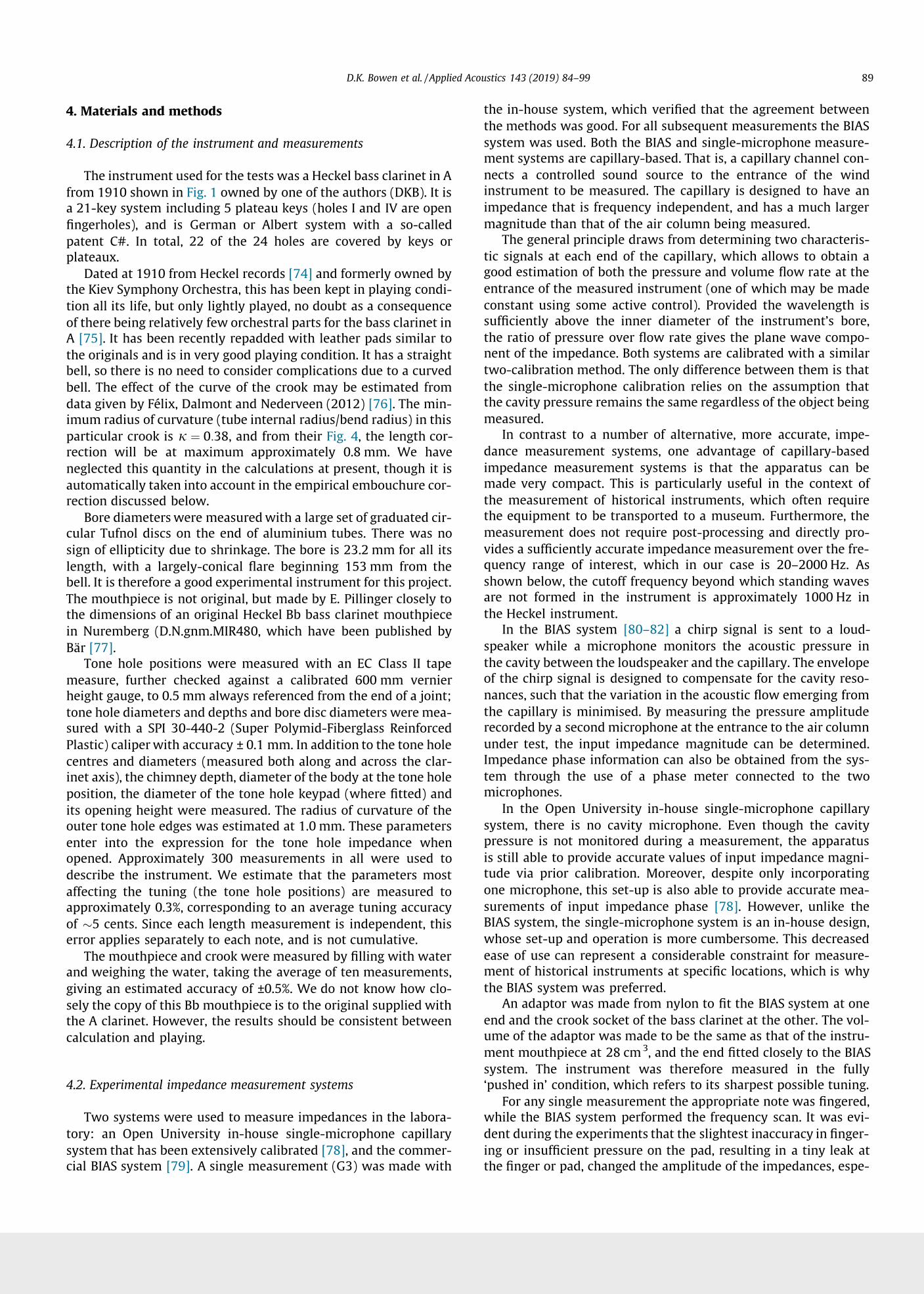
The

instrument used for the tests was a Heckel bass clarinet in

Afrom 1910 shown in owned by one of

the authors (DKB). It isFig. 1a 21-key system including 5 plateau keys

(holes I and IV are openfingerholes), and is German

or Albert system

with a so-calledpatent C#. In total, 22 of the 24 holes are covered by keys orplateaux.

Dated at

1910 from Heckel records

and formerly owned by[74]the Kiev Symphony Orchestra, this has been kept in playing condi-tion all its life, but only

lightly played, no doubt as a consequenceof there being relatively few orchestral parts for the bass clarinet inA . It has been recently repadded with leather pads similar to[75]the originals and is in very good playing condition. It has a straightbell, so there is no need to consider complications due to a curvedbell. The effect of the curve of the crook may be estimated fromdata given by Félix, Dalmont and Nederveen (2012) . The min-[76]imum radius of curvature (tube internal radius/bend radius) in thisparticular crook is j ¼ 0 38, and from their , the length cor-: Fig. 4rection will be at

maximum approximately 0.8 mm. We haveneglected

this quantity in the calculations at present, though it isautomatically

taken

into account in the empirical embouchure cor-rection discussed below.

Bore diameters were measured with a large set of graduated cir-cular

Tufnol discs on the end of aluminium tubes. There was nosign of ellipticity due to shrinkage. The bore is 23.2 mm for all itslength, with a largely-conical flare beginning 153 mm from thebell. It is therefore a good experimental instrument for this project.The mouthpiece is not original, but made by E. Pillinger closely tothe dimensions of an original Heckel Bb

bass clarinet mouthpiecein Nuremberg (D.N.gnm.MIR480, which have been published byBär .[77]

Tone hole positions were measured with an EC Class II tapemeasure, further checked against a calibrated 600 mm vernierheight gauge, to 0.5

mm always

referenced from the end of a joint;tone hole diameters and depths and bore disc diameters were mea-sured with a SPI 30-440-2 (Super Polymid-Fiberglass ReinforcedPlastic) caliper with accuracy ±

0.1 mm. In addition to the tone holecentres and diameters (measured both along and across the clar-inet axis), the chimney depth, diameter of the body at

the tone holeposition, the diameter of the tone hole

keypad (where fitted) andits opening height were measured. The radius of curvature of theouter tone hole edges was estimated at

1.0 mm. These parametersenter

into the expression for the tone hole impedance whenopened. Approximately 300 measurements in all were used todescribe the instrument. We estimate that the parameters

mostaffecting the tuning (the tone hole positions) are measured toapproximately 0.3%, corresponding to an average tuning accuracyof 5

cents. Since each length measurement is independent, this

error applies separately to each note, and is not cumulative.The

mouthpiece and crook were measured by filling

with

waterand weighing the water,

taking the average of ten measurements,giving an estimated accuracy of ±0.5%. We do not know how clo-sely the copy of this Bb mouthpiece is to the original supplied withthe A clarinet. However, the results should be consistent betweencalculation and playing.

4.2. Experimental impedance measurement systems

Two systems were used to measure impedances in the labora-tory: an Open University in-house single-microphone capillarysystem that has been extensively calibrated , and the commer-[78]cial BIAS system . A single measurement (G3) was made with[79]

the in-house system, which verified that the agreement betweenthe methods was good. For all subsequent measurements the BIASsystem was used. Both the BIAS and single-microphone measure-ment systems are capillary-based. That is, a capillary channel

con-nects a controlled sound source to the entrance of the windinstrument to be

measured. The capillary

is designed to have animpedance that is frequency independent, and has a much largermagnitude than that of the air column

being measured.The general principle draws from determining two characteris-

tic signals at each end of the capillary, which allows to obtain agood estimation of both the pressure and volume

flow rate at theentrance of the measured instrument (one of which may be madeconstant using some active control). Provided the wavelength

issufficiently above the inner diameter of the instrument’s bore,the ratio of pressure over flow rate gives the plane wave compo-nent of the impedance. Both

systems are calibrated with a similartwo-calibration method. The only difference between them is thatthe single-microphone calibration relies on the assumption thatthe cavity pressure remains the same regardless

of the object beingmeasured.

In contrast to a number of alternative, more accurate, impe-dance measurement systems, one advantage of capillary-basedimpedance measurement systems is that the apparatus can bemade very compact. This is particularly useful in the context ofthe measurement of historical instruments, which often requirethe equipment to be transported to a museum. Furthermore, themeasurement does not require post-processing and directly pro-vides a sufficiently accurate impedance measurement over the fre-quency range of interest, which in our case

is 20–2000 Hz. Asshown below, the cutoff frequency beyond which standing wavesare not formed in the instrument is approximately 1000 Hz inthe Heckel instrument.

In the BIAS

system a chirp signal is sent to a loud-[ ]80–82speaker while a microphone monitors the acoustic pressure inthe cavity between the loudspeaker and the capillary. The envelopeof the chirp signal is designed to compensate for the cavity reso-nances, such that the variation in the acoustic flow emerging fromthe capillary is minimised. By measuring the pressure

amplituderecorded by a second microphone at the entrance to the air columnunder test, the input impedance magnitude can be determined.Impedance phase information can also be obtained from the sys-tem through the use of a phase meter connected to the twomicrophones.

In the Open University in-house single-microphone capillarysystem, there is no cavity

microphone. Even though the cavitypressure is not monitored during a measurement, the apparatusis still able to provide accurate values of input impedance magni-tude via prior calibration. Moreover, despite only incorporatingone microphone, this set-up is also able to provide accurate mea-surements of input impedance phase . However, unlike the[78]BIAS system, the single-microphone system is an in-house design,whose set-up and operation is more cumbersome. This decreasedease of use can represent a considerable constraint for measure-ment of historical instruments at

specific locations, which is whythe BIAS system was preferred.

An adaptor was made from nylon to fit

the BIAS system at oneend and the crook socket of the bass clarinet at the other. The vol-ume of the adaptor was made to be the same as that of the instru-ment mouthpiece at 28 cm 3, and the end fitted closely to the BIASsystem. The instrument was therefore measured in the fully‘pushed in’ condition, which refers to its sharpest possible tuning.

For any single measurement the appropriate note was fingered,while the BIAS system performed the frequency scan. It was evi-dent during the experiments that the slightest inaccuracy in finger-ing

or insufficient pressure on the pad, resulting in a tiny leak atthe finger or pad, changed the amplitude of the impedances, espe-

D.K. Bowen et al. / Applied Acoustics 143 (2019) 84–99 89

cially that of the first resonance

peak,

quite drastically. Each

mea-surement was therefore repeated after relaxing the

fingering, tocheck that the two scans were essentially identical. This empha-sizes the point made in , that the instrument must be inSection 1good, leak-free condition for meaningful impedancemeasurements.

4.3. Audio frequency measurements

In order to compare the measured and calculated impedanceswith

the pitches actually produced, the instrument was

played(after warming up), and the sounds recorded over chromatic scales.Each note was played for several seconds, without looking at atuner and while attempting to play in the natural ‘centre’ of eachnote. Two sets of recordings were made, one with the mouthpiecepushed in (corresponding to the

acoustic measurement conditions)and the other

with the

mouthpiece pulled out 10.8 mm, the max-imum practical on this instrument, to attempt correction of theperceived sharpness

when referred to A4 =

440 Hz. Recordingwas made in a ‘dry’ acoustic room (though not an anechoic cham-ber) with a Rode NT1A microphone (20 Hz–20 kHz) , using an AkaiEIE Pro interface

and Logic Pro X

software, at 24 bit 44.1 kHz.

Theresulting WAV files were segmented into sections for each note,each at least 4

s long after

truncating the transients at the begin-nings and ends of the note

to leave a steady tone portion. The fre-quency was determined in MatLab TM using the YIN algorithm .[83]The accuracy of this method is estimated by its authors to beapproximately ±1 cent, which is much better than

can be obtainedby

digital Fourier transform methods.

5. Results

5.1. Comparison of calculations and acoustic measurements

The tone-hole cutoff frequency

for this instrument is about1000 Hz, calculated from Benade’s formula for an open tone-[10]hole lattice

f c ¼ 0 11: cb

a

1sl

1 2=

ð Þ2

where f c is the cutoff frequency, the speed of sound, the pipec a

radius, the hole radius, the hole spacing

and the acoustic lengthb s l

of the holes. Clearly this is an approximation, since the hole spac-ings and diameters do vary somewhat, but it is confirmed by visualinspection of the impedance spectra. It is

worth noting this value,since for bass clarinets, and also by scaling from soprano clarinets,one would normally expect a

cutoff around 750 Hz . This[ , ]10 73could be a significant parameter to evaluate in the study of histor-ical instruments,

since it definitely affects the musical sound andplaying qualities, as discussed by Benade , who notes that[10]woodwind instruments have actually ‘evolved’ over the centuriesso that their cutoff frequencies became approximately constantover the

whole

range of the instrument. Waves with

frequenciesbeyond the cutoff limit are not reflected at the first open tone holebut transmit through to and out of the bell (which is designed tohave a similar cutoff frequency). They thus do not contribute to

the standing waves in the instrument nor to the feedback that sta-bilises the oscillations of the reed, though they can contribute(weakly) to the sound spectrum. We thus chose the frequency range20–2000 Hz, with 0.5 Hz steps, for both the measurements and cal-culations. The range on the instrument for analysis was chosen tobe from written E2 to D5 (69.3–494 Hz fundamental frequencies),corresponding to C#2 to B4 concert pitches. Whilst informationcould be obtained from higher note fingerings. It is less significant;only one resonance frequency contributes to defining the pitch pro-duced for notes above about G4, and this pitch can be varied widelyby embouchure control in the altissimo regime. In this regime thepitch of the sound produced is more

reliant

on the skill of the playerthan on the instrument.

To

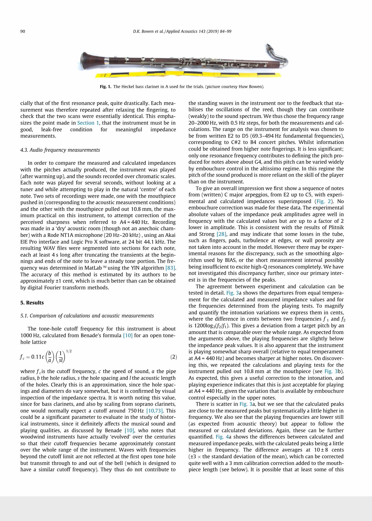
give an overall impression we first show a sequence

of notesfrom (written) C major arpeggios, from E2 up to C5, with experi-mental and calculated impedances superimposed ( ). NoFig. 2embouchure correction was made for these data. The experimentalabsolute values of the

impedance peak amplitudes agree well infrequency with the calculated values but are up to a factor of 2lower in amplitude. This is consistent with the results of Plitnikand

Strong , and may indicate that some losses in the tube,[28]such as fingers, pads, turbulence at edges, or wall porosity arenot taken into account in the model. However there may be exper-imental reasons for

the discrepancy, such as the smoothing algo-rithm used by BIAS, or the short measurement interval possiblybeing insufficient

to excite

high-Q resonances completely. We havenot investigated this discrepancy further, since our primary inter-est is in the frequencies

of the peaks.The agreement between experiment and

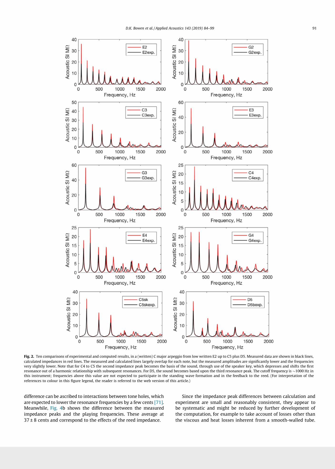
calculation

can betested in detail. a shows the departures from equal tempera-Fig. 3ment for the calculated and measured impedance values and forthe frequencies determined from the playing tests. To magnifyand

quantify the intonation variations we express them in cents,where the difference in cents between two frequencies f 1 and f 2

is 1200log 2(f 2 /f1). This gives a deviation from a target pitch by anamount that is comparable over the whole range. As expected fromthe arguments above, the playing

frequencies are slightly belowthe impedance peak values. It is

also apparent that the instrumentis playing somewhat sharp overall

(relative to equal temperamentat A4 = 440 Hz) and becomes

sharper at higher notes. On discover-ing this, we repeated the calculations and playing tests for theinstrument pulled out 10.8 mm

at the mouthpiece (see b).Fig. 3As expected, this gives a useful correction to

the intonation, andplaying experience indicates that this is just acceptable for playingat A4 = 440 Hz, given the variation that is available by embouchurecontrol especially in the upper notes.

There is scatter in a, but we see that the calculated peaksFig. 3are close to the measured peaks but systematically a little higher infrequency. We also

see that the playing frequencies are lower still(as expected from acoustic theory) but appear to follow themeasured or calculated deviations. Again, these can be furtherquantified. a shows the differences between

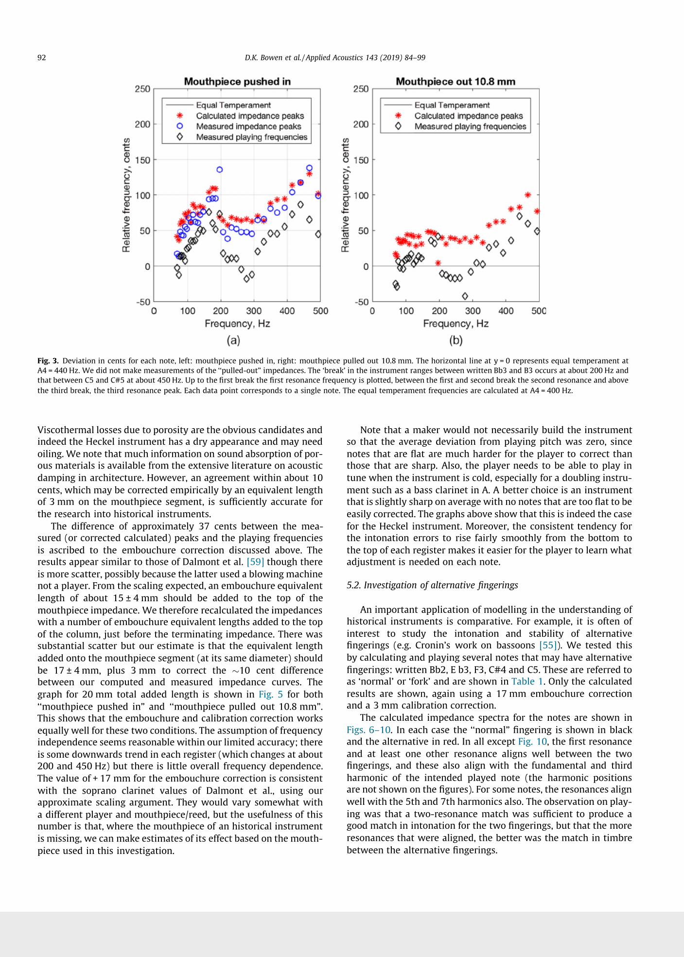
calculated andFig. 4measured impedance peaks, with the calculated peaks being a littlehigher in frequency. The difference averages at 10 ± 8 cents(±3 the standard deviation of the mean), which can be corrected

quite well with a 3 mm calibration correction added to the mouth-piece length (see below). It is possible that at least some of this

Fig. 1. The Heckel bass clarinet in A

used for the trials. (picture courtesy Huw

Bowen).

90 D.K. Bowen et al. / Applied Acoustics 143 (2019) 84–99

difference can be ascribed to interactions between tone holes, whichare expected to lower the resonance frequencies by a few cents [71].Meanwhile, b shows the difference between the measuredFig. 4impedance peaks and the

playing frequencies. These average at37 ± 8 cents and correspond to the effects of the reed impedance.

Since

the impedance peak differences between calculation andexperiment are small and reasonably consistent, they appear tobe systematic and might be reduced by further development ofthe computation, for example to

take account of losses other thanthe viscous and heat losses inherent from a smooth-walled tube.

Fig. 2. Ten comparisons of experimental and computed results, in a (written) C major arpeggio from low written E2 up to C5 plus D5. Measured data are shown in black lines,calculated impedances in red lines. The measured and calculated lines largely overlap for each note, but the measured

amplitudes are significantly lower and the

frequenciesvery slightly lower. Note that for C4 to C5 the second impedance peak becomes the basis of the sound, through use of

the speaker key, which depresses and shifts the firstresonance out of a harmonic relationship with subsequent resonances. For D5, the sound becomes based upon the third resonance peak. The cutoff frequency is 1000 Hz in

this instrument; frequencies above this value are not expected to participate in the standing wave formation and in the feedback to the reed. (For interpretation of thereferences to colour in this figure legend, the reader is referred to the web version of this article.)

D.K. Bowen et al. / Applied Acoustics 143 (2019) 84–99 91

Viscothermal losses due to porosity are the obvious candidates andindeed the Heckel instrument has a dry appearance and may needoiling. We note that much information on sound absorption of por-ous materials is available

from the extensive literature on acousticdamping in architecture. However, an agreement within about 10cents, which may be corrected empirically by an equivalent lengthof 3 mm on the mouthpiece segment, is sufficiently accurate forthe research into historical instruments.

The difference of approximately 37 cents between the mea-sured (or corrected calculated) peaks and the playing frequenciesis ascribed to the embouchure correction discussed above. Theresults appear similar to those of Dalmont et al.

though

there[59]is more scatter, possibly because the

latter used a blowing machinenot a player. From the scaling expected, an embouchure equivalentlength of about 15 ± 4 mm should be added to the top of themouthpiece impedance. We therefore recalculated the impedanceswith

a number of embouchure equivalent lengths added to the topof the column, just before the terminating impedance. There

wassubstantial scatter but our estimate is

that the equivalent lengthadded onto the mouthpiece segment (at its same diameter) shouldbe 17 ± 4 mm, plus 3 mm to correct the 10 cent difference

between our computed and measured

impedance curves. Thegraph for 20 mm total added length is shown in for bothFig. 5‘‘mouthpiece pushed in” and ‘‘mouthpiece pulled out 10.8 mm”.This shows that the embouchure and calibration correction worksequally well for these two conditions. The assumption of frequencyindependence seems reasonable within our limited accuracy; thereis some downwards trend in each register (which changes at about200 and 450 Hz) but

there is little overall frequency dependence.The value of + 17 mm for the embouchure correction is consistentwith

the soprano clarinet values of Dalmont et al., using ourapproximate scaling argument. They would vary somewhat witha different player and mouthpiece/reed, but the usefulness

of thisnumber is that, where the mouthpiece of an historical instrumentis missing, we can make estimates of its

effect based on the mouth-piece used

in this

investigation.

Note that a maker would not necessarily

build the instrumentso that

the average deviation from playing pitch was zero, sincenotes that are flat are much harder for the player to correct thanthose that are sharp. Also,

the player needs to be able to play intune when the instrument is cold, especially for a doubling instru-ment such

as a bass clarinet in A. A better choice is an instrumentthat is slightly sharp on average with no notes that are too

flat to beeasily corrected. The graphs above show that

this is indeed the casefor the Heckel instrument. Moreover, the consistent tendency forthe intonation errors to rise fairly smoothly from the bottom tothe top of each register makes it easier for the player to learn whatadjustment is needed on each note.

5.2. Investigation of alternative fingerings

An important application of modelling in the understanding ofhistorical instruments is comparative. For

example, it is often ofinterest to study the intonation and stability of alternativefingerings (e.g. Cronin’s work on bassoons ). We tested this[55]by calculating and playing several notes that may have alternativefingerings: written Bb2, E b3, F3, C#4 and C5. These are referred toas ‘normal’ or ‘fork’ and are shown in . Only the calculatedTable 1results are shown, again using a 17 mm embouchure correctionand

a 3 mm calibration correction.The calculated impedance spectra for the notes are shown in

Figs. 6–10. In each case the ‘‘normal” fingering is shown in blackand

the alternative in red.

In all except , the

first resonanceFig. 10and

at least one other resonance aligns well between the twofingerings, and these also align with the fundamental and thirdharmonic of the intended played note (the

harmonic positionsare not shown on the figures). For some notes, the resonances alignwell with the 5th and 7th harmonics also. The observation on play-ing was that a two-resonance match

was sufficient to produce agood match in intonation for the two fingerings, but that the moreresonances that were aligned, the better was the match in timbrebetween the alternative fingerings.

Fig. 3. Deviation in cents for each note, left: mouthpiece pushed in, right: mouthpiece pulled out 10.8 mm. The horizontal line at y = 0 represents equal temperament atA4 = 440 Hz. We did not make measurements of the ‘‘pulled-out” impedances. The

‘break’ in the instrument ranges between written

Bb3 and B3 occurs at about 200 Hz andthat between C5

and C#5 at about 450 Hz. Up to the first break the first resonance frequency is plotted, between the first and second break the second resonance and abovethe third break, the third resonance peak. Each data point corresponds to a single note. The equal temperament frequencies are calculated at A4 = 400 Hz.

92 D.K. Bowen et al. / Applied Acoustics 143 (2019) 84–99

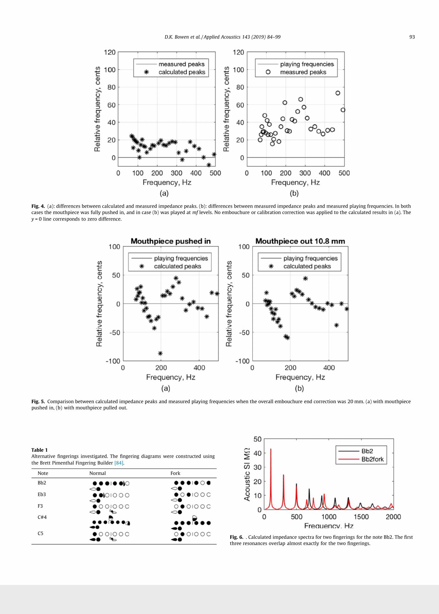
Fig. 4. (a): differences between calculated and measured impedance peaks. (b): differences between measured impedance peaks and measured playing frequencies. In bothcases the mouthpiece was fully pushed in, and in case (b) was played at levels. No embouchure or calibration correction was applied to the calculated results in (a). Themf

y = 0 line corresponds to zero difference.

Fig. 5. Comparison between calculated impedance peaks and measured playing frequencies when the overall embouchure end correction was 20 mm. (a) with mouthpiecepushed in, (b) with mouthpiece pulled out.

Table 1

Alternative fingerings investigated. The fingering diagrams were constructed

usingthe Brett Pimenthal Fingering

Builder .[84]

Note Normal Fork

Bb2

Eb3

F3

C#4

C5Fig. 6. . Calculated impedance spectra for two fingerings for the note Bb2. The firstthree resonances overlap

almost exactly for the two fingerings.

D.K. Bowen et al. / Applied Acoustics 143 (2019) 84–99 93

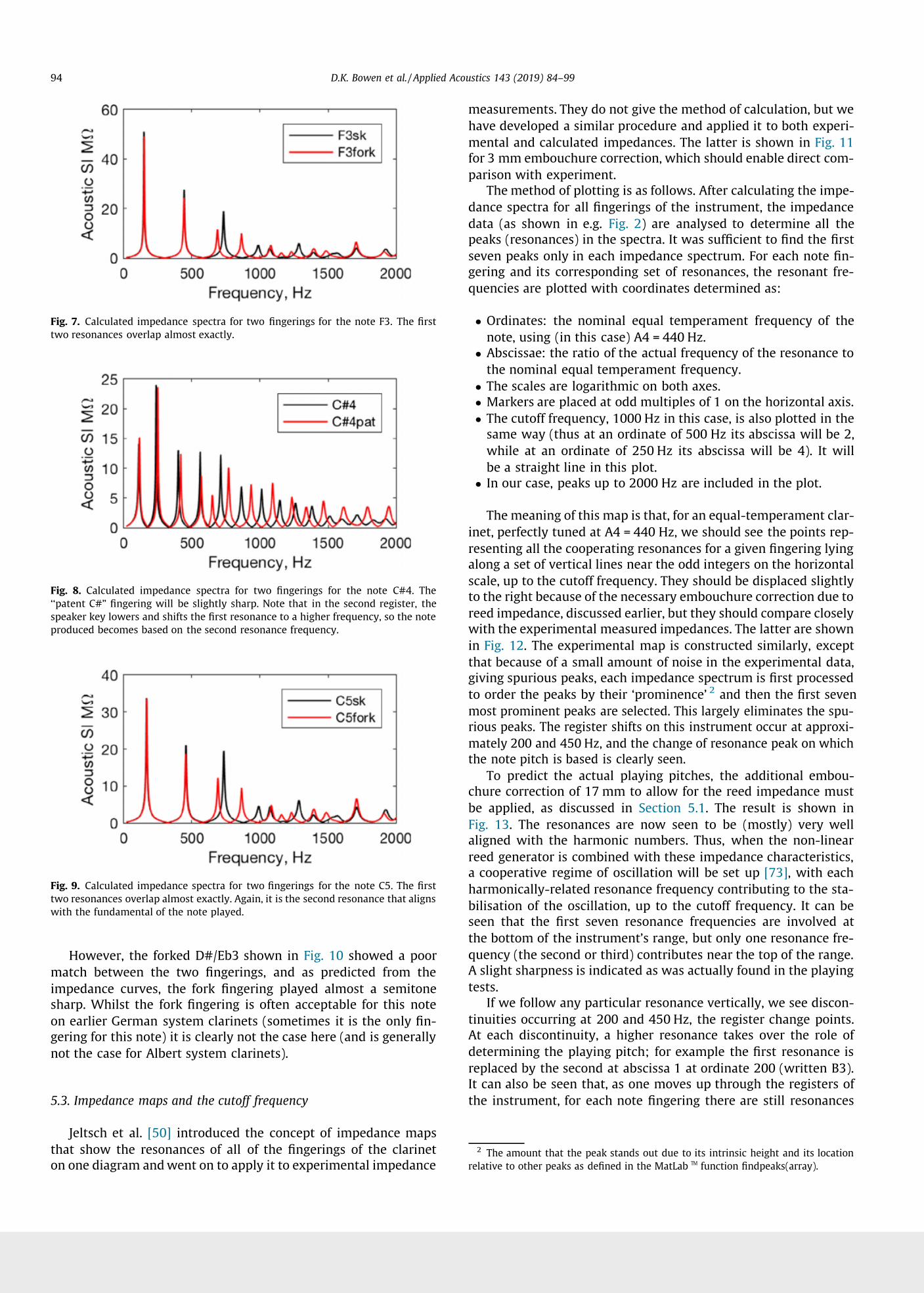
However, the forked D#/Eb3 shown in showed a

poorFig. 10match between the two fingerings, and as predicted from theimpedance curves, the fork fingering played almost a semitonesharp. Whilst the

fork fingering is often acceptable for this noteon earlier German system clarinets (sometimes it is

the only fin-gering for this note) it is clearly not the case here (and is generallynot the case for Albert system

clarinets).

5.3. Impedance maps and the cutoff frequency

Jeltsch et al.

introduced

the concept of impedance maps[50]that show the resonances of all of the fingerings of the clarineton one diagram and went on to apply it to experimental impedance

measurements. They do not give

the method of calculation, but wehave developed a similar procedure and applied it to both experi-mental and

calculated impedances. The latter is shown in Fig. 11for 3 mm

embouchure correction, which should enable direct com-parison with experiment.

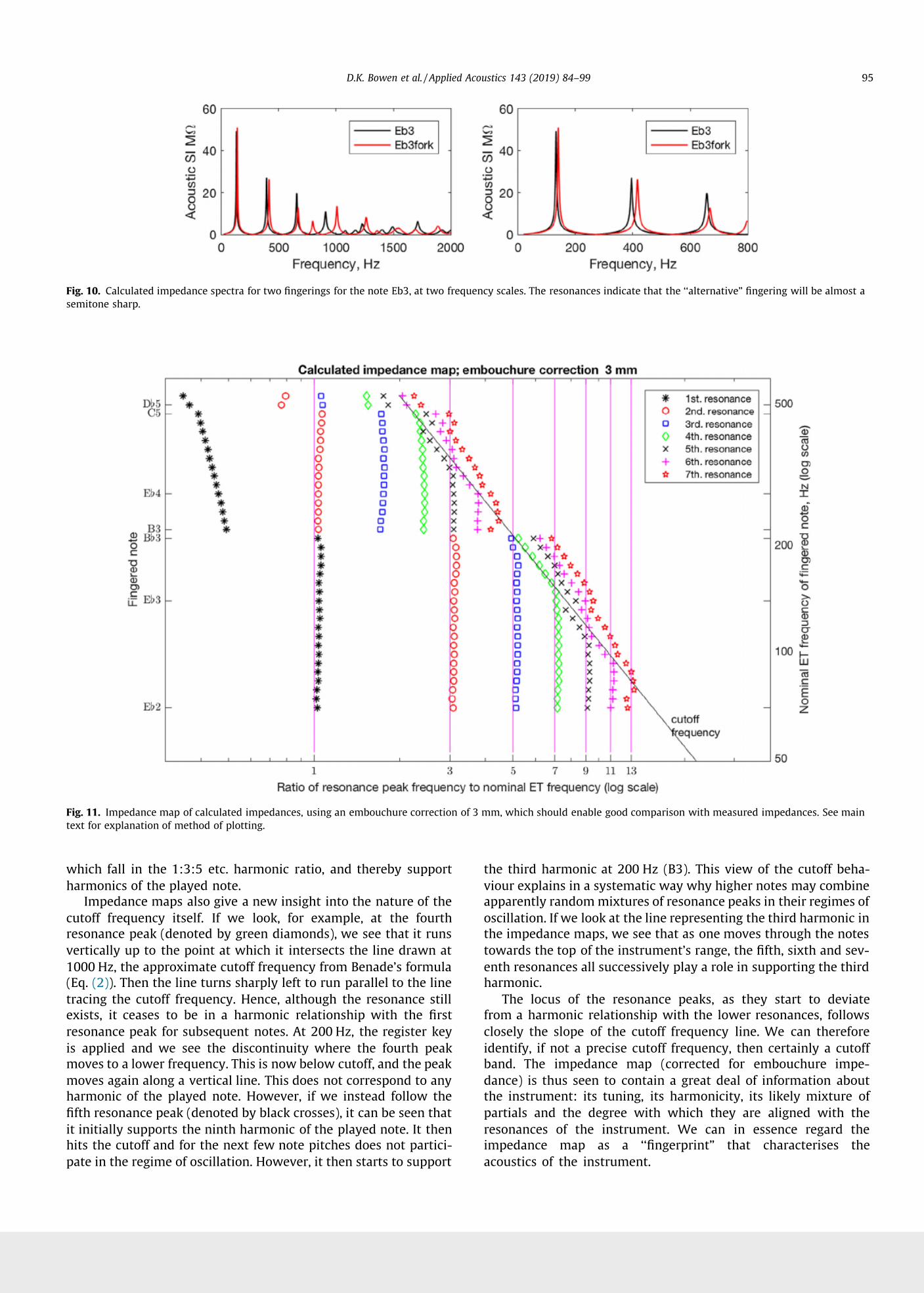
The method of plotting is as follows. After calculating the impe-dance spectra for

all fingerings of the instrument, the impedancedata (as shown in e.g. ) are analysed to determine all theFig. 2peaks

(resonances) in the spectra. It was sufficient to find the firstseven

peaks only in each impedance spectrum. For each note fin-gering and its corresponding set of resonances, the resonant fre-quencies are plotted with coordinates determined as:

Ordinates: the nominal equal

temperament frequency of thenote, using (in this case) A4 = 440 Hz.

Abscissae: the ratio of the actual frequency of the resonance tothe nominal equal temperament frequency.

The scales are logarithmic on both axes. Markers are placed at odd multiples of 1 on the horizontal axis. The cutoff frequency,

1000 Hz in this case,

is also plotted in thesame way (thus at an ordinate of 500 Hz its abscissa will be 2,while at an ordinate of 250 Hz its abscissa will be 4). It willbe a straight line in this plot.

In our case, peaks up to 2000 Hz are included in the plot.

The meaning of this map is that, for an equal-temperament clar-inet, perfectly

tuned at A4 = 440

Hz, we should see the points rep-resenting all the cooperating resonances

for a given fingering lyingalong a set of vertical

lines near the odd integers on the horizontalscale, up to the cutoff

frequency. They should be displaced slightlyto the right because of the necessary embouchure correction due toreed impedance, discussed earlier, but they should compare closelywith the experimental measured impedances. The latter are shownin . The experimental map is constructed similarly, exceptFig. 12that because of a small amount of noise in the experimental data,giving

spurious peaks, each impedance

spectrum is first processedto order the peaks by their ‘prominence’ 2 and then the first sevenmost prominent peaks are selected. This largely eliminates the spu-rious peaks. The register shifts on this instrument occur at approxi-mately 200 and 450 Hz, and the change of resonance peak on whichthe note pitch is based is clearly seen.

To

predict

the

actual playing pitches, the additional embou-chure correction

of 17 mm to allow

for the reed impedance mustbe applied, as discussed in . The result is shown inSection 5.1Fig. 13. The

resonances are now seen to be (mostly) very wellaligned with the harmonic numbers. Thus, when the non-linearreed generator is combined with these impedance characteristics,a cooperative regime of oscillation will be set up , with each[73]harmonically-related resonance frequency contributing to the sta-bilisation of the oscillation, up to the cutoff frequency.

It can beseen that the first seven resonance frequencies are involved atthe bottom of the instrument’s range,

but

only one resonance fre-quency (the second or third) contributes near the top of the range.A slight sharpness is indicated as was actually found in the playingtests.

If we follow any particular resonance vertically, we

see discon-tinuities

occurring at 200

and 450 Hz, the

register change points.At

each discontinuity, a higher resonance takes over the role ofdetermining the playing pitch; for example the first resonance isreplaced by the second at abscissa 1 at ordinate 200 (written B3).It can also be seen that, as one moves up through the

registers ofthe instrument, for each note fingering there are still resonances

Fig. 7. Calculated impedance spectra for two fingerings for the note F3. The firsttwo resonances overlap almost exactly.

Fig. 8. Calculated impedance spectra for two

fingerings for the note C#4. The‘‘patent C#” fingering will be slightly sharp. Note that in the second register, thespeaker key lowers and shifts the first resonance to a higher frequency, so the noteproduced becomes based on the second resonance frequency.

Fig. 9. Calculated impedance spectra for two fingerings for the note C5. The firsttwo resonances overlap almost exactly. Again, it is the second resonance that alignswith the fundamental of the note played.

2 The amount that the peak stands out due to its intrinsic height and its locationrelative to

other peaks as defined in the MatLab TM function findpeaks(array).

94 D.K. Bowen et al. / Applied Acoustics 143 (2019) 84–99

which fall in the 1:3:5 etc. harmonic ratio,

and thereby supportharmonics of the played note.

Impedance maps also give a new insight into the nature of thecutoff frequency itself. If we look, for example, at the fourthresonance peak (denoted by green diamonds), we see that it runsvertically up to the point at which it intersects the line

drawn at1000 Hz, the approximate cutoff frequency from Benade’s formula(Eq. ). Then the line turns sharply left to run parallel to the line(2)tracing the cutoff frequency. Hence, although the resonance stillexists, it ceases to be in a harmonic relationship with the firstresonance peak for subsequent notes. At 200 Hz, the register keyis applied and we see the discontinuity where the fourth peakmoves

to a lower frequency. This is now below cutoff, and the peakmoves

again along a vertical line. This does not correspond to anyharmonic of the played note. However, if we instead follow thefifth resonance peak (denoted by black crosses), it can be seen thatit initially supports the ninth harmonic of the

played note. It thenhits the cutoff and for the next

few note pitches does not partici-pate in the regime of oscillation. However, it then starts to support

the third harmonic at 200 Hz (B3). This view of the cutoff

beha-viour explains in a systematic way why higher notes may combineapparently random mixtures of resonance peaks in their regimes ofoscillation. If we look at the line representing the third harmonic

inthe impedance maps, we see that as one moves through the notestowards the top of the

instrument’s range, the fifth, sixth and sev-enth resonances

all successively play a role

in

supporting the thirdharmonic.

The locus of the resonance peaks, as they start to deviatefrom a harmonic relationship

with the lower resonances, followsclosely the slope of the cutoff

frequency line.

We can thereforeidentify, if not a precise cutoff frequency, then certainly a cutoffband. The impedance map (corrected for embouchure impe-dance) is thus seen to contain a great deal of information aboutthe instrument: its tuning, its harmonicity, its likely mixture ofpartials and the degree with which they are aligned with theresonances of the instrument. We can in essence regard

theimpedance map as a ‘‘fingerprint” that characterises theacoustics of the instrument.

Fig. 11. Impedance map of calculated impedances, using an embouchure

correction of 3 mm, which should enable good comparison with measured impedances. See maintext for explanation of method of plotting.

Fig. 10. Calculated impedance spectra for two fingerings for the note Eb3, at two frequency scales. The

resonances indicate that the ‘‘alternative” fingering will

be almost asemitone sharp.

D.K. Bowen et al. / Applied Acoustics 143 (2019) 84–99 95

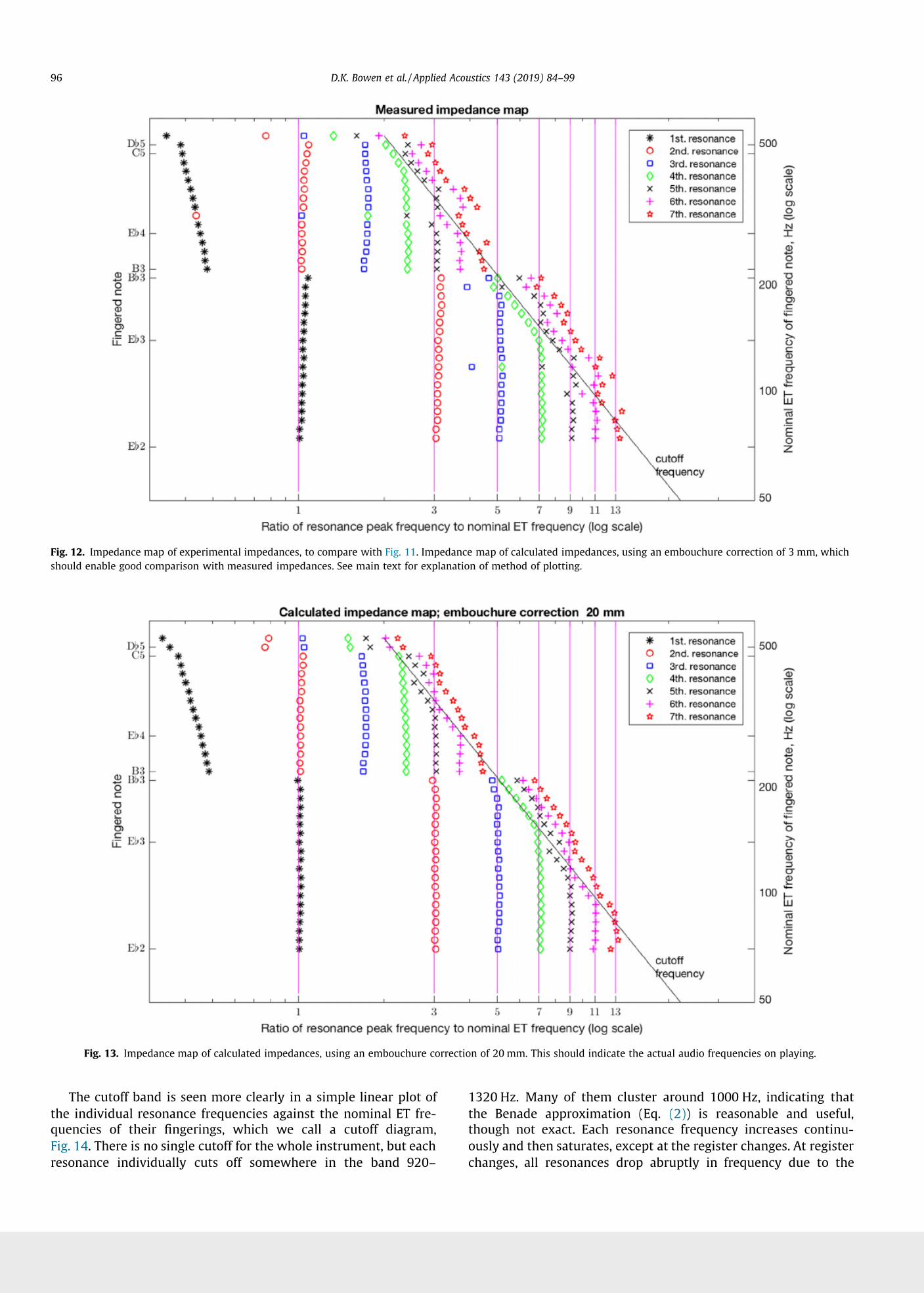
The cutoff band is

seen more clearly in a simple linear plot ofthe individual resonance frequencies

against the nominal ET fre-quencies of their fingerings, which we call a cutoff diagram,Fig.

14. There is no single cutoff for the whole instrument, but eachresonance individually cuts off somewhere in

the band 920–

1320 Hz. Many of them cluster around 1000 Hz, indicating

thatthe Benade approximation (Eq. ) is reasonable and useful,(2)though not exact. Each resonance frequency increases continu-ously and then saturates, except at the register changes. At registerchanges, all resonances drop abruptly in frequency due to the

Fig. 13. Impedance map of calculated impedances, using an embouchure correction of 20 mm. This should indicate the actual audio frequencies on playing.

Fig. 12. Impedance map of experimental impedances, to compare with . Impedance map of calculated impedances, using an embouchure correction of 3 mm, whichFig. 11should enable good comparison with measured impedances. See main text for explanation of method of plotting.

96 D.K. Bowen et al. / Applied Acoustics 143 (2019) 84–99

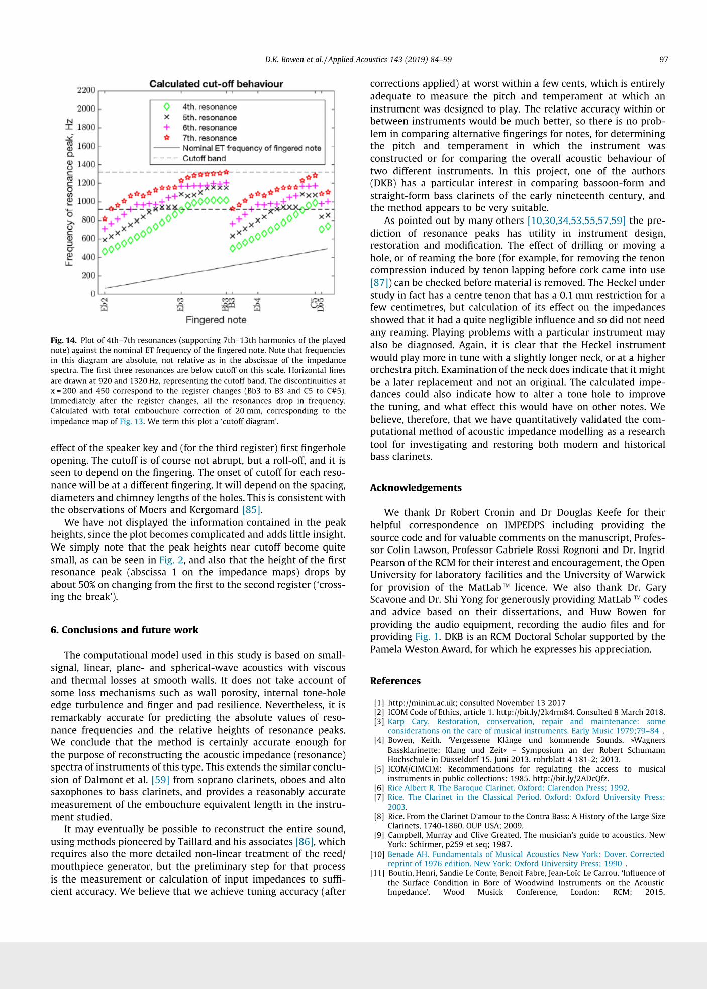
effect of the

speaker key and (for the third register) first fingerholeopening. The cutoff is of course not abrupt, but a roll-off, and it isseen to depend on the fingering. The onset of cutoff for each reso-nance will be at a different fingering. It will depend on the spacing,diameters and chimney lengths of the

holes. This is consistent withthe observations of Moers and Kergomard .[85]

We have not displayed the information contained in the peakheights, since the plot becomes complicated and adds little insight.We simply note that the peak heights near cutoff become quitesmall, as can be seen in , and also that the height of the firstFig. 2resonance peak (abscissa 1 on the impedance maps) drops byabout 50% on changing from the first to the second register (‘cross-ing the break’).

6. Conclusions and future work

The

computational model

used in this

study is

based on small-signal, linear, plane- and spherical-wave acoustics with viscousand thermal losses at smooth

walls. It does not take account ofsome loss mechanisms such as wall porosity, internal tone-holeedge turbulence and finger and pad resilience. Nevertheless, it isremarkably accurate for predicting the absolute values of reso-nance frequencies and

the relative heights of resonance peaks.We conclude that the method is certainly accurate enough forthe purpose of reconstructing the acoustic impedance (resonance)spectra

of instruments of this type. This extends the similar conclu-sion of Dalmont et al. from soprano clarinets, oboes and alto[59]saxophones to bass clarinets, and provides a reasonably accuratemeasurement of the embouchure equivalent length in the instru-ment

studied.It

may eventually be possible to reconstruct the entire sound,using methods pioneered by Taillard and his associates , which[86]requires also the more detailed non-linear treatment of the reed/mouthpiece generator, but the preliminary step for that processis the

measurement or calculation of input impedances to suffi-cient accuracy. We believe that we achieve tuning accuracy (after

corrections applied) at worst within a few cents, which is entirelyadequate to measure the pitch and temperament at which aninstrument was designed to play. The relative accuracy within orbetween instruments would be much better, so there is no prob-lem in comparing alternative fingerings for notes, for determiningthe pitch and temperament in which the instrument wasconstructed or for comparing the overall acoustic behaviour oftwo

different instruments. In this project, one of the authors(DKB) has a particular interest in comparing bassoon-form andstraight-form bass clarinets of the early nineteenth century, andthe method appears to be very suitable.

As pointed out by many others the

pre-[ , , , , , , ]10 30 34 53 55 57 59diction of resonance peaks has utility in instrument design,restoration and modification. The effect of drilling or moving ahole, or of reaming the bore (for example, for removing the tenoncompression induced by tenon lapping before cork came into use[87]) can be checked before material is removed. The Heckel understudy in fact has a centre tenon that has

a 0.1 mm restriction for afew centimetres, but calculation of its effect on the impedancesshowed that it had a quite negligible influence and so did not needany

reaming. Playing problems with a particular instrument mayalso be diagnosed. Again, it is clear that the Heckel instrumentwould play more in tune with a slightly longer neck, or at a higherorchestra pitch. Examination of the

neck does indicate that it mightbe a later

replacement

and not an original. The calculated impe-dances could also indicate how to alter a tone hole to improvethe tuning, and what effect this would have on other notes. Webelieve, therefore, that we have quantitatively validated the com-putational method of acoustic impedance modelling as a researchtool for investigating and restoring both modern and historicalbass clarinets.

Acknowledgements

We thank Dr Robert Cronin and Dr Douglas Keefe for theirhelpful correspondence on IMPEDPS including providing thesource code and

for valuable comments on the manuscript, Profes-sor Colin Lawson, Professor Gabriele Rossi Rognoni and Dr. IngridPearson of the RCM for their interest and

encouragement, the OpenUniversity for laboratory facilities

and the University of Warwickfor provision

of the MatLab TM licence. We also thank Dr. GaryScavone and Dr.

Shi Yong for generously providing MatLab TM codesand advice based on their dissertations, and Huw Bowen forproviding the audio equipment, recording

the audio files and forproviding . DKB is an RCM Doctoral Scholar supported by theFig. 1Pamela Weston Award, for

which he expresses his appreciation.

References

[1] http://minim.ac.uk; consulted November 13 2017[2] ICOM

Code of Ethics, article 1. http://bit.ly/2k4rm84. Consulted 8 March 2018.[3] Karp Cary. Restoration, conservation, repair and maintenance: some

considerations on the care of musical instruments. Early

Music 1979;79–84 .[4] Bowen, Keith. ‘Vergessene Klänge und kommende Sounds. »Wagners

Bassklarinette: Klang und Zeit« – Symposium an der Robert SchumannHochschule in Düsseldorf 15. Juni 2013. rohrblatt 4 181-2; 2013.

[5] ICOM/CIMCIM: Recommendations for regulating the access to musicalinstruments in public collections: 1985. http://bit.ly/2ADcQfz.

[6] Rice Albert R. The Baroque Clarinet. Oxford: Clarendon Press; 1992.[7] Rice. The Clarinet in the Classical Period. Oxford: Oxford University Press;

2003.[8] Rice. From the Clarinet D’amour to

the Contra Bass: A History of the Large SizeClarinets, 1740-1860. OUP USA; 2009.

[9] Campbell, Murray and Clive Greated, The musician’s guide to acoustics. NewYork: Schirmer, p259 et seq; 1987.

[10] Benade AH. Fundamentals of Musical Acoustics New York: Dover. Correctedreprint of 1976 edition. New York: Oxford University Press; 1990 .

[11] Boutin, Henri, Sandie Le Conte, Benoit Fabre, Jean-Loïc Le Carrou. ‘Influence ofthe Surface Condition in Bore of Woodwind Instruments on the AcousticImpedance’. Wood Musick Conference, London: RCM; 2015.

Fig. 14. Plot of 4th–7th resonances (supporting 7th–13th harmonics of the playednote)

against the nominal ET frequency of the fingered note. Note that frequenciesin this diagram are absolute, not relative as in the abscissae of the impedancespectra. The first three resonances are below cutoff on this scale. Horizontal linesare drawn at 920 and 1320 Hz, representing the cutoff band. The discontinuities atx = 200 and 450 correspond to the

register changes (Bb3 to B3 and C5 to C#5).Immediately after the register changes, all the resonances drop in frequency.Calculated with total embouchure correction of 20 mm, corresponding to theimpedance map of . We term this plot a ‘cutoff diagram’.Fig. 13

D.K. Bowen et al. / Applied Acoustics 143 (2019) 84–99 97

http://woodmusick.org/wp-content/uploads/COST%20Conference%20booklet%20London.pdf.

[12] Smith RA, Mercer DMA. Possible causes of woodwind tone colour. J Sound Vib1974;32:347–58 .

[13] Benade Arthur H. Horns, strings and harmony. New York: Anchor; 1960.[14] Carral Sandra, Vergez Christophe, Nederveen

Cornelis J. Toward a single reedmouthpiece for an oboe. Archiv Acoust 2011;36:267–82 .

[15] Helmholtz, Hermann von. Tonempfindungen. (1863). Tr. Alexander J. Ellis. Onthe sensations of tone. (1954) New York: Dover reprint.

[16] Bouasse, H. Instruments à Vent (Vol. I and II).

Paris: Libraire Delagrove; 1929.[17] Lamb H. Dynamical theory of sound. London: E. Arnold; 1910.[18] Olson HF. Acoustical engineering. Princeton: Van Nostrand; 1957.[19] Caussé R, Kergomard J, Lurton X. Input impedances of brass musical

instruments. J Acoust Soc Am 1984;75:241–54 .[20] Backus J. Small vibration theory of the clarinet. J Acoust Soc Am

1963;35:305–13 .[21] Strutt JW. The theory of sound (2 nd Baron Rayleigh). London: Macmillan and

Co; 1877 .[22] McGinnis CS, Gallagher C. The mode of vibration of a clarinet reed. J Acoust Soc

Am 1941;12:529–31 .[23] Taillard Pierre-André, Kegomard Jean. An analytical prediction of the

bifurcation scheme of a clarinet-like instrument: effects of resonator losses.Acta Acustica united with Acustica 2015;101:279–91 .

[24] Levine

Harold, Schwinger Julian. On the radiation of sound from an unflangedcircular pipe. Phys Rev 1948;73:383–406 .

[25] Dalmont J-P, Nederveen CJ, Joly N. Radiation impedance of tubes with differentflanges: numerical

and experimental investigations. J Sound Vib 2001;244(3):505–34 .

[26] Worman, Walter E. Self-Sustained Nonlinear Oscillations in Clarinet-LikeSystems. Ph.D. diss., Case Western Reserve University, Cleveland, Ohio; 1971.

[27] Chaigne Antoine, Kergomard Jean. Acoustics of musical instruments (1 st

English edition). New York:

Springer-Verlag; 2016 .[28] Plitnik GR, Strong WJ. Numerical method for

calculating input impedances ofthe oboe. J Acoust Soc Am 1979;65:816–25 .

[29] Keefe DH. Woodwind air column models. J Acoust Soc Am 1990;88:35–51.[30] Nederveen CJ. Acoustical aspects of woodwind instruments (revised

edition). Dekalb, IL: Northern University Illinois Press; 1998 .[31] Guillemain P, Kergomard J, Voinier T. Real-time synthesis of clarinet-like

instruments using digital impedance models. J Acoust Soc Am2005;118:483–94 .

[32] Scavone Gary P, Smith Julius O. A stable acoustic impedance model of theclarinet using digital waveguides Sep. 18-20. Proc. Of the 9 th InternationalConference on Digital Audio Effects (DAFx-06), Montreal, Canada, 2006 .

[33] Bolton, Philippe. ‘Resonans: a software program for developing new windinstruments. FOMRHI QUARTERLY, 79

69-72; 1995 (Communication No.1356).

[34] Scavone Gary Paul. An acoustic analysis of single reed woodwind instrumentswith an emphasis on design

and performance issues and digital waveguidemodeling techniques PhD Thesis. Stanford University; 1997 .

[35] Yong Shi. Comparing Theory and Measurements of Woodwind-LikeInstrument Acoustic Radiation MA Thesis. Montreal: McGill University; 2009 .

[36] Benade AH, Kouzoupis

SN. The clarinet spectrum: theory and experiment. JAcoust Soc Am 1988;83:292–304 .

[37] Benade Arthur H, Keefe Douglas H. Galpin Soc J 1996;49:113–42.[38] Benade, A.H. ‘Benade’s NX clarinet: Its genesis’ (written in 1987 and published

posthumously), The Clarinet; Jan/Feb 1994, p. 46–8.[39] Jameson, George. ‘Benade’s clarinet:

Mechanical and other considerations. TheClarinet;

May/June 1994, p. 32–3.[40]

Stephen Fox Clarinets. http://www.sfoxclarinets.com/Benade.html. Consulted8 March 2018.

[41] Dalmont J-P. Acoustic impedance measurement, part i: review. J Sound Vib2001;243:427–39 .

[42] Dalmont J-P. Acoustic impedance measurement, part ii: review. J Sound Vib2001;243:441–59 .

[43] Kausel,

W. and Kuehnelt H. ‘A practical way to measure intonation quality ofwoodwind instruments using standard equipment without custom madeadaptors’. Acoustics ’08, Paris. (www.acoustics08-paris.org).

[44] Widholm G.,

Pichler H.,

Ossmann T. ‘BIAS: a computer-aided test system forbrass wind instruments’. An Audio Engineering Society Preprint;

1989, 2834.[45] https://www.ircam.fr/project/detail/pafi/consulted 22 November 2017.[46] Sharp DB. Acoustic pulse

reflectometry for the measurement of musical windinstruments PhD Thesis. The University of Edinburgh; 1996 .

[47] Sharp DB. Increasing the length of tubular object that can be measured usingacoustic pulse reflectometry. Meas Sci Technol 1998;9:1469–79 .

[48] Li A, Sharp DB, Forbes BJ. Increasing the axial resolution of

bore profilemeasurements made using acoustic pulse reflectometry. Measur Sci Technol2005;16:2011–9 .

[49] Campbell, Murray ‘‘Acoustical Evaluation of Historic Wind Instruments”Forum Acusticum 2005 Budapest; Acta acustica united with Acustica, 91Supplement; 2005.

[50] Jeltsch Jean, Gibiat Vincent, Forest L. Acoustical Study of a Set of Six KeyBaumann’s Clarinets.

In: Proc. International Symposium

on MusicalInstruments (Dourdan, 1995). p. 134–40 .

[51] Lefevre Jean-Xavier, de Clarinette Méthode. Adopté Par Le Conservatoire PurServir À l’étude Dans Cet Établissement. Paris: Impr. du Conservatoire deMusique; 1802 .

[52] Jeltsch, Jean and Nicholas Shackleton, ‘‘Caractéristation Acoustique de TroisClarinettes de Facteurs Lyonnais,” in Colloque Acoustique et InstrumentsAnciens: Factures, Musiques et Science (Colloque Acoustique et InstrumentsAnciens: Factures, Musiques et Science, Paris: Cité de la Musique, 1999),p. 103–24.

[53] Schumacher RT. calculations of the oscillations of a clarinet. AcusticaAb Initio

1981;48:71–85 .[54] Backus J. Input impedance for reed woodwind instruments. J Acoust Soc Am

1974;56:1266–79 .[55] Cronin Robert H. Understanding the operation of auxiliary fingerings on the

modern bassoon. J Int Double Reed Soc 1996;24:13–30 .[56] Cronin, Robert and Douglas Keefe. ‘Understanding the operation of auxiliary

fingerings on conical doublereed instruments’. Unpublished notes for a talkpresented at the 131st meeting of the Acoustical Society of America,Indianapolis, Indiana; 13-17 May 1996.

[57] Dart Mathew. The Baroque Bassoon: form, construction, acoustics, and playingqualities. London: London Metropolitan University; 2011. PhD thesis .

[58] Hichwa, Bryant and David Rachor. ‘In-depth acoustic modeling andtemperament studies of

18th and early 19th century baroque bassoonscomparing originals and reproductions by maker, time period, and region’.Société Francaise d’Acoustique. Acoustics 2012, Apr 2012, Nantes, France;2012. Online: <hal-00810841>

[59] Dalmont JP, Gazengel B, Gilbert J, Kergomard J. Some aspects of tuning andclean intonation in reed instruments. Appl Acoust 1995;46:19–60 .

[60] Mamou-Mani A, Sharp DB. Evaluating the suitability of acousticalmeasurement techniques and psychophysical testing for studying theconsistency

of musical wind instrument manufacturing. Appl Acoust2010;71:668–74 .

[61] Mamou-Mani A, Sharp DB, Meurisse T, Ring W. Investigating the consistencyof woodwind instrument manufacturing by comparing five nominallyidentical oboes. J Acoust Soc Am 2012;131(1):728–36 .

[62] Kowal, Paulina; Sharp, David and Taherzadeh, Shahram. ‘Analysing

differencesbetween the input impedances of five clarinets of different makes’. In:Institute of Acoustics Annual Spring Conference 2013: Acoustics 2013, 13

May2013,

Nottingham, UK; 2013.[63] Hélie Thomas, Rodet Xavier. Radiation of a pulsating portion of a sphere:

application to horn radiation. Acta Acustica United with Acustica2003;89:565–77 .

[64] Benade AH, Murday JS. Measured end corrections for woodwind tone holes. JAcoust Soc Am 1967;41:1609 .

[65] Fletcher Neville H, Rossing Thomas D. The physics of musical instruments. 2nded. New York: Springer; 2010 .

[66] Kulik Yakov. Transfer matrix of conical waveguides with any geometricparameters for increased precision in computer modeling. J Acoust Soc Am2007;122(5):EL179 .

[67] Grothe Thimo. Experimental Investigation of Bassoon Acoustics Dr,-Ingthesis. Technical University of Dresden; 2014 .

[68] Nederveen, C.J., J. K. M. Jansen, and R. R. van Hassel, ‘‘Corrections forWoodwind Tone-Hole Calculations,” Acta Acustica United with Acustica 84,no. 5 (September 1, 1998), p. 957–66.

[69] Dubos V, Kergomard J, Khettabi A, Dalmont J-P, Keefe DH, Nederveen CJ.Theory of sound propagation in a duct with a branched tube using modaldecomposition. Acta Acustica

(Stuttgart) March

1999;85(2):153–69 .[70] Dalmont J-P, Nederveen CJ, Dubos V, Ollivier S, Vincent Meserette V, te Sligte E.

Experimental determination of the equivalent circuit of an open side hole:linear and non linear behaviour. Acta Acustica united with Acustica2002;88:567–75. 9 .

[71] Lefebvre Antoine, Scavone Gary P, Kergomard Jean. External toneholeinteractions in woodwind instruments. Acta Acustica United with Acustica2013;99:975–85 .

[72] Thompson Stephen C. The effect of the reed resonance on woodwind toneproduction. J Acoust

Soc Am 1979;66:1299–307 .[73] Benade AH, Gans DJ. Sound production in wind instruments. Ann N Y Acad Sci

1968;155:247–63 .[74] Reiter Edith. Wilhelm Heckel, six generations dedicated to

music. Wiesbaden: Marixverlag; 2014 .[75] Bowen, D. Keith. ‘The Rise and

Fall of the Bass Clarinet in A’, The Clarinet;September 2011, p. 44-1; 2011.

[76] Félix Simon, Dalmont Jean-Pierre, Nederveen CJ. Effects of bending portions ofthe air column on the acoustical resonances of a wind instrument. J Acoust SocAm 2012;131(5):4164–72. https://doi.org/10.1121/1.3699267

https://doi.org/10.1121/1.3699267

https://doi.org/10.1121/1.3699267

https://doi.org/10.1121/1.3699267

https://doi.org/10.1121/1.3699267

https://doi.org/10.1121/1.3699267

https://doi.org/10.1121/1.3699267

https://doi.org/10.1121/1.3699267

https://doi.org/10.1121/1.3699267 .[77] Bär, Frank P. Verzeichnis der Europäischen Musikinstrumente in

Gemanischen Nationalmuseum Nürnberg. Band

6: Liebesklarinetten,Bassetthörner, Bassklarinetten, Metallklarinetten. Wilmhelmshaven: FlorianNoetzel; 2006.

[78] Sharp D, Mamou-Mani A, Van Walstijn M. A single microphone capillary-basedsystem for measuring the complex input impedance of musical windinstruments. Acta Acust United Ac 2011;97. 819–829(5) .

[79] Widholm G, Pichler H, Ossmann T. BIAS A computer-aided test system forbrass wind instruments. Audio Eng Soc 1989 .

[80] Widholm G, Winkler W. Evaluation of musical instrument quality by computersystems ISBN: 91845289876. In: Examples of realisation’, Proceedings of theSMAC93. Royal Swedish Academy of Music; 1994. p. 560–5 .

[81] Widholm G. Brass wind instrument quality measured and evaluated by a newcomputer system Trondheim, Norway (June 26–30, 1995). In: Proceedings ofthe 15th International Congress

on Acoustics. p. 517–20 .

98 D.K. Bowen et al. / Applied Acoustics 143 (2019) 84–99

[82] Kausel W. Bore reconstruction of

tubular ducts from its acoustic inputimpedance curve. IEEE Trans Instrum Meas August 2004;53(4):1097–105.https://doi.org/10.1109/TIM.2004.831440

https://doi.org/10.1109/TIM.2004.831440

https://doi.org/10.1109/TIM.2004.831440

https://doi.org/10.1109/TIM.2004.831440

https://doi.org/10.1109/TIM.2004.831440

https://doi.org/10.1109/TIM.2004.831440

https://doi.org/10.1109/TIM.2004.831440

https://doi.org/10.1109/TIM.2004.831440

https://doi.org/10.1109/TIM.2004.831440 .[83] de Cheveigne Alain, Kawahara Hideki. YIN a fundamental frequency estimator

for speech and music. J Acoust Soc Am 2002;111:1917–30 .[84] Pimentel, Brett, Fingering Diagram Builder, https://fingering.

bretpimentel.com/#!/clarinet-german/albert/. Consulted 11 March 2018.[85] Moers Elise, Kergomard Jean. On the cutoff frequency

of clarinet-likeinstruments. Geometrical versus acoustical regularity.

Acta Acustica Unitedwith Acustica 2011;97:984–96. https://doi.org/10.3813/AAA.918480

https://doi.org/10.3813/AAA.918480

https://doi.org/10.3813/AAA.918480

https://doi.org/10.3813/AAA.918480

https://doi.org/10.3813/AAA.918480

https://doi.org/10.3813/AAA.918480

https://doi.org/10.3813/AAA.918480

https://doi.org/10.3813/AAA.918480

https://doi.org/10.3813/AAA.918480 .

[86] Taillard, Pierre-André, Fabrice Silva and Philippe Guillemain, ‘Simulation entemps réel de l’impédance d’entrée mesurée ou calculée des instruments àvent’. Conference CFA/VISHNO April 2016; available on ResearchGate.

[87] McGee, Terry. ‘Effect of thread wrapping on flute tenons’ http://www.mcgee-flutes.com/effects_of_thread_wrapping.htm (2011). Consulted 20/11/2017.

D.K. Bowen et al. / Applied Acoustics 143 (2019) 84–99 99