A

cTfiysTwap©

K

1

lasatticadi

(

0d

Analytica Chimica Acta 596 (2007) 171–182

Exploring groundwater hydrochemistry of alluvial aquifersusing multi-way modeling

Kunwar P. Singh ∗, Amrita Malik, Sarita Sinha 1,Dinesh Mohan, Vinod Kumar Singh

Environmental Chemistry Division, Industrial Toxicology Research Centre, Post Box 80, MG Marg, Lucknow 226001, India

Received 16 November 2006; received in revised form 1 June 2007; accepted 1 June 2007Available online 3 June 2007

bstract

A three-way data set pertaining to hydrochemistry of the groundwater of north Indo-Gangetic alluvial plains was analyzed using three-wayomponent analysis method with the purpose of extracting the information on spatial and temporal variation trends in groundwater composition.hree-way data modeling was performed using PARAFAC and Tucker3 models. The models were tested for their stability and goodness of optimalt using core consistency diagnostic and split-half analysis. Although, a two-component PARAFAC model, explaining 50.47% of data variance,ielded 100% core consistency, it failed to qualify the validation test. Tucker3 model (3, 3, 1) captured 55.18% of the data variance and yieldedimple diagonal core with three significant elements, explaining 100% of the core variability. Interpretation of the information obtained throughucker3 model revealed that the groundwater quality in Khar watershed is mainly dominated by water hardness and related variables, whereas,

ater composition of the dug wells is dominated by alkalinity and carbonate/bicarbonates. Moreover, shallow groundwater sources in the region

re contaminated with nitrate derived from fertilizers application in the region. The shallow aquifers are relatively more contaminated during theost-monsoon season.

2007 Elsevier B.V. All rights reserved.

round

ftr

tsa[lac

eywords: Multi-way modeling; Component analysis; PARAFAC; Tucker3; G

. Introduction

Hydrochemistry of groundwater aquifer in a region isargely determined by both the natural processes, suchs precipitation, wet and dry depositions of atmosphericalts, evapo-transpiration, soil/rock–water interactions, and thenthropogenic activities, which can alter these systems by con-aminating them or by modifying the hydrological cycle. Bothhe natural processes, as well as the anthropogenic activities varyn time and space; which are reflected in groundwater hydro-hemistry variations, show spatial and temporal fluctuations in

region. Alluvial regions are more accessible to such variationsue to high population densities and intense agricultural andndustrial activities. Understanding of the factors responsible

∗ Corresponding author. Tel.: +91 522 2508916; fax: +91 522 2628227.E-mail addresses: kpsingh 52@yahoo.com, kunwarpsingh@gmail.com

K.P. Singh).1 National Botanical Research Institute, Lucknow.

aaw1iniGa

003-2670/$ – see front matter © 2007 Elsevier B.V. All rights reserved.oi:10.1016/j.aca.2007.06.001

water; Hydrochemistry; Indo-Gangetic plains

or influencing the groundwater hydrochemistry is very essen-ial for protection and sound management of the groundwateresources in a region.

Alluvial aquifers constitute a hydrological unit formed byhe alluvial deposits, which are characterized by a linear andhallow feature. The shallow character and high permeability oflluvial aquifers make them highly vulnerable to contamination1]. In our case, the study area in vicinity of the Ganga river isocated in the industrial belt between Kanpur, an industrial townnd Lucknow, the state capital of Uttar Pradesh. The study area,omprising of both the younger and older alluvium regions, hasthree-tier aquifer system. Vertically, clay and sand occur as

lternate bands of varying thickness. Groundwater occurs underater table conditions and depth to water varies between 1 and2 m round the year. The water table gradient of 0.8–1.0 m km−1

n the region indicates gentle slope depicting the permeable

ature of shallow aquifer horizon [2]. Further, the study regions well known for high fluoride levels in soils and water [2–4].roundwater in this region is used for domestic, agricultural

nd industrial purposes. Therefore, the study of the groundwa-

1 himic

trm

aorfec

reM(evidtmramobunTUcoabsts

bamsotlapi

2

tim

X

a

x

wm(ntu

X

w|rP(m

((

x

wArGaeCtta

X

wrPchoosing different number of factors in different modes [22,24].The original core (G) may be rotated to optimize for super-diagonality (Gd) and to maximize the core variance (Gv) in orderto obtain a matrix with a limited number of elements having highabsolute values, thus making the relation between them moreunderstandable [23,25]. The constrained Tucker model due to its

72 K.P. Singh et al. / Analytica C

er hydrochemistry, its spatial and temporal variations in theegion has been considered as of priority importance for safeanagement of groundwater resources.Water quality databases due to large number of variables usu-

lly have complex multivariate structure. Such databases areften difficult to analyze with meaningful interpretation andequire data reduction methods to simplify the data structureor extracting useful and interpretable information which couldxplain the spatial and temporal variation patterns of the hydro-hemical variables.

Multivariate statistical methods provide powerful tools foresolution and modeling of large multivariate data arrays gen-rated through environmental monitoring programmes [5,6].ultivariate methods, such as principal component analysis

PCA), a variable reduction procedure capable of providing anasy visualization of relationships existing among objects orariables in large and/or complex databases can provide datanterpretation [7–10]. However, the water quality monitoringata sets, generally exhibit multi-dimensional structure (space,ime, and variables), which require multi-way (N-way) analysis

ethods to explore and extract the hidden data structure and theirelationships. Among these, multi-way (principal) componentnalysis methods have been emerging with growing interest. Theulti-way principal component analysis (MPCA), an extension

f PCA to higher orders, designed to deal with multi-way data isased on a classical PCA performed on an unfolded data matrixnder an orthogonality constraint [11]. The multi-way compo-ent analysis performed through the PARAFAC [12–14] anducker [15,16] models also deals with multi-way data analysis.nlike MPCA, PARAFAC and Tucker models are hierarchi-

al methods as their parameters change when different numbersf components are calculated [17]. The multi-way componentnalysis models devised with this purpose have successfullyeen applied to the study of N-way problems of different areas,uch as spectroscopy [12], food chemistry [18] and environmen-al studies [19–23] and employed to interpret multi-array dataets.

This paper aims to present a three-way component modeluilt from a three-dimensional data array (sampling sites, vari-bles, sampling seasons) generated through groundwater qualityonitoring in alluvial region of north Indian Gangetic plains,

ampled during the pre- and post-monsoon seasons over a periodf 3 years (2003–2005) at 62 sites (Fig. 1). In the present study,he three-way data set of groundwater hydrochemistry was ana-yzed by three-way component analysis using the PARAFACnd Tucker3 models with a view to evaluate the spatial and tem-oral variation trends and major hydro-geo-chemical processesn the alluvial region.

. Theory

Multi-way analysis of data having multi-dimensional struc-ure can provide more in-depth and relevant information for

nterpretation of the results. PARAFAC and Tucker3 models are

ainly used for multi-way analysis of data.The PARAFAC method decomposes the three-way data array,(I × J × K) in to three loadings matrices, A (I × F), B (J × F)

rttc

a Acta 596 (2007) 171–182

nd C (K × F) as [12];

ijk =F∑

f=1

aif bjf ckf + eijk (1)

here xijk is the j-scaled data array; aif, bjf and ckf are the ele-ents of the three loadings matrices, A, B, and C of (nobj × F),

nvar × F) and (ncond × F) dimensions, respectively, F is theumber of factors extracted for each mode, and eijk is the errorerm of the elements of data set. Eq. (1) for three-way array X,nfolded as X (I × JK), can also be written as:

(I×JK) = A(C| ⊗ |B)T + EX (2)

here matrices A, B, and C represent the loadings as above,⊗| is the Khatri-Rao product and EX is the matrix of modelesiduals of dimension (I × JK). The consecutive modes of theARAFAC model are obtained by the alternating least squaresALS) approach [12]. The PARAFAC is a constrained Tucker3odel with same number of factors, F for each loadings matrix.In Tucker3 model, the original three-way data array, X

I × J × K) is decomposed in to three loadings matrices, AI × P), B (J × Q), C (K × R), and a core matrix as below [16],

ijk =P∑

p=1

Q∑

q=1

R∑

r=1

aipbjqckrgpqr + eijk (3)

here aip, bjq, and ckr are the elements of the loadings matrices,, B, and C of (nobj × P), (nvar × Q) and (ncond × R) dimensions,

espectively; gpqr denotes the elements (p, q, r) of the core array(P × Q × R), and eijk is the error term of the j-scaled X data

rray. The squared element (g2pqr) of the core reflects the variance

xplained by the interactions among the three modes (A, B, and), and P, Q, and R are the number of factors extracted from the

hree different modes, chosen as small as possible. Eq. (3) forhree-way unfolded data array, X (I × JK), can also be writtens;

(I×JK) = AG(C ⊗ B)T + EX (4)

here ⊗ is the Kronecker product, EX is the matrix of modelesiduals, and G is the core array, G (P × Q × R) arranged as× QR. A major advantage with Tucker model is its flexibility in

otational freedom is not structurally unique, which means thathe rotation of A, B, C and G matrices do not imply the change ofhe model fit. This emphasizes for straightforward interpretableore array obtained for the selected model of complexity [26].

himic

3

3

vlSdab[w4sa(f

iaTaa1

a2aeTaf

K.P. Singh et al. / Analytica C

. Experimental

.1. Study area

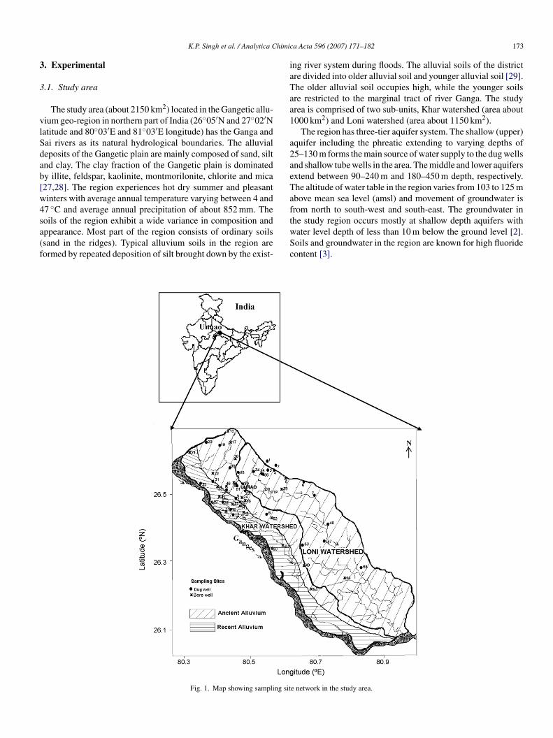
The study area (about 2150 km2) located in the Gangetic allu-ium geo-region in northern part of India (26◦05′N and 27◦02′Natitude and 80◦03′E and 81◦03′E longitude) has the Ganga andai rivers as its natural hydrological boundaries. The alluvialeposits of the Gangetic plain are mainly composed of sand, siltnd clay. The clay fraction of the Gangetic plain is dominatedy illite, feldspar, kaolinite, montmorilonite, chlorite and mica27,28]. The region experiences hot dry summer and pleasantinters with average annual temperature varying between 4 and7 ◦C and average annual precipitation of about 852 mm. The

oils of the region exhibit a wide variance in composition andppearance. Most part of the region consists of ordinary soilssand in the ridges). Typical alluvium soils in the region areormed by repeated deposition of silt brought down by the exist-

twSc

Fig. 1. Map showing sampling sit

a Acta 596 (2007) 171–182 173

ng river system during floods. The alluvial soils of the districtre divided into older alluvial soil and younger alluvial soil [29].he older alluvial soil occupies high, while the younger soilsre restricted to the marginal tract of river Ganga. The studyrea is comprised of two sub-units, Khar watershed (area about000 km2) and Loni watershed (area about 1150 km2).

The region has three-tier aquifer system. The shallow (upper)quifer including the phreatic extending to varying depths of5–130 m forms the main source of water supply to the dug wellsnd shallow tube wells in the area. The middle and lower aquifersxtend between 90–240 m and 180–450 m depth, respectively.he altitude of water table in the region varies from 103 to 125 mbove mean sea level (amsl) and movement of groundwater isrom north to south-west and south-east. The groundwater in

he study region occurs mostly at shallow depth aquifers withater level depth of less than 10 m below the ground level [2].oils and groundwater in the region are known for high fluorideontent [3].

e network in the study area.

1 himic

3

arsttd22tsgw

cowpicpt

cd[d(((r(oC7Mcrs(ia3udbmlcaiw

dd

wpbna

3

pbotss

×wcva[itTa(ve

3

Large environmental data arrays containing concentrationinformation on multiple chemical compounds collected at dif-ferent sampling periods from different sampling sites arranged

74 K.P. Singh et al. / Analytica C

.2. Sampling and analytical procedures

The sampling network and strategy were designed to coverwide range of determinants at key sites, which reasonably

epresent the groundwater quality in the study region. In thistudy, the representative sampling sites were chosen in ordero cover various agricultural and industrial activities (Fig. 1). Aotal of 96, 80, 79 and 94 samples of groundwater were collecteduring the post-monsoon (October 2003); pre-monsoon (June004), pre-monsoon (June 2005), and post-monsoon (October005) seasons, respectively. Here, we have selected only 62 ofhese samples, which were collected from common samplingites during all the four samplings over 3 years. Among the 62roundwater samples, 34 were collected from bore wells (boreells, tube wells, hand pumps) and 28 from the open dug wells.Samples from tube wells, bore wells and hand-pumps were

ollected from the outlets after flushing water for 10–15 min inrder to remove the stagnant water. Samples from the dug wellsere collected using water sampler. All the samples collected inre-cleaned tight-capped high quality polyethylene bottles weremmediately transported to the laboratory under low temperatureonditions in ice-boxes and stored in the laboratory at 4 ◦C untilrocessed/analyzed. All analyses were completed within a weekime.

The measured variables included the characteristic hydro-hemical parameters of groundwater. All the parameters wereetermined in laboratory following the standard protocols30]. The samples were analyzed for pH, electrical con-uctivity (EC), total dissolved solids (TDS), total alkalinityT-Alk), bicarbonate (HCO3), carbonate (CO3), total hardnessT-Hard), calcium hardness (Ca-Hard), magnesium hardnessMg-Hard), nitrate–nitrogen (NO3–N), chloride (Cl), fluo-ide (F), sulfate (SO4), sodium (Na), potassium (K), calciumCa), and magnesium (Mg). Major anions viz. chloride, flu-ride, sulfate and nitrate were analyzed using modular Ionhromatograph (Metrohm, Switzerland) having a Metrohm IC-09 programmable pump, Metrohm IC-733 separation centre,etrohm IC-753 suppressor module and a Metrohm IC-732

onductivity detector. The separation was achieved on a met-osep anion dual column with an eluent composed of mixedodium carbonate (1.3 mmol L−1) and sodium bicarbonate2.0 mmol L−1). The flow rate was kept 1.0 ml min−1 with annjection volume of 20 �l. Among the major cations, sodiumnd potassium were analyzed by Flame Photometer (model CL-60, Elico, India), while calcium and magnesium were analysedsing AAS (model Analyst 300, Perkin-Elmer, USA). TDS wereetermined gravimetrically, while alkalinity, bicarbonate, car-onate and hardness by acid–base titration method. The pH waseasured using a pH-meter (model 744, Metrohm, Switzer-

and). Electrical conductivity was measured at 25 ◦C with aonductivity meter (model 162A, Thermo-Orion, USA). All thenalytical equipments were regularly calibrated. All the chem-cals, reagents and standards used in various estimations [30]

ere of analytical grade.The analytical data quality was ensured through careful stan-

ardization, procedural blank measurements, and spiked anduplicate samples. The ionic charge balance of each sample was

a Acta 596 (2007) 171–182

ithin ±5%. The laboratory also participates in regular nationalrogram on analytical quality control (AQC). In all the analysis,lanks were run and corrections were applied to the results, ifecessary. All the observations were recorded in duplicate andverage values are reported.

.3. Preprocessing of data

Shapiro–Wilk test was applied to check the distributionattern of the variables. All the variables showed a skewed distri-ution and therefore, a logarithmic transformation was appliedn them. Non-normal distribution is very usual in environmen-al data, and the logarithmic transformation is commonly usedince it allows one to obtain a normal distribution from highlykewed data [31].

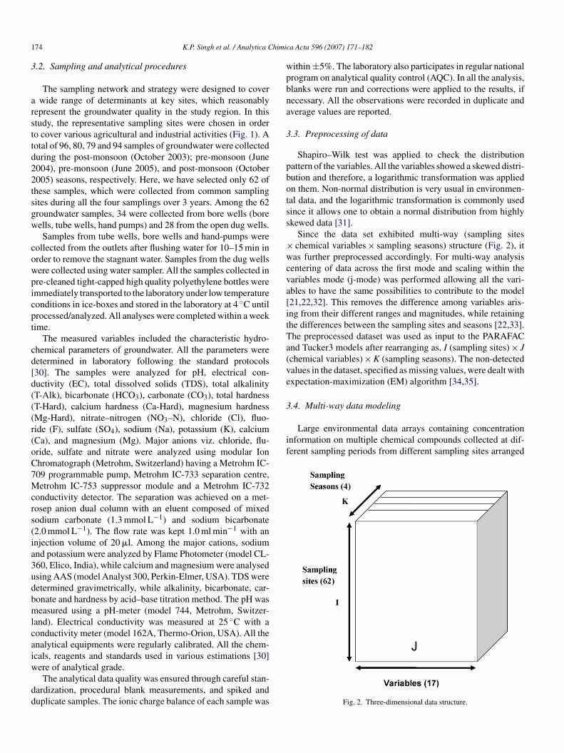
Since the data set exhibited multi-way (sampling siteschemical variables × sampling seasons) structure (Fig. 2), itas further preprocessed accordingly. For multi-way analysis

entering of data across the first mode and scaling within theariables mode (j-mode) was performed allowing all the vari-bles to have the same possibilities to contribute to the model21,22,32]. This removes the difference among variables aris-ng from their different ranges and magnitudes, while retaininghe differences between the sampling sites and seasons [22,33].he preprocessed dataset was used as input to the PARAFACnd Tucker3 models after rearranging as, I (sampling sites) × Jchemical variables) × K (sampling seasons). The non-detectedalues in the dataset, specified as missing values, were dealt withxpectation-maximization (EM) algorithm [34,35].

.4. Multi-way data modeling

Fig. 2. Three-dimensional data structure.

himic

iasddwTm7t(vaaaFtemo

3

tasmgnmtTtmuficddoaCtssIast

tiaatou

CtsetsnTyttebwctsC(cfmtl

3

aata

h

h

h

wo

atooocsa.

m(vi

K.P. Singh et al. / Analytica C

n large tables, data matrices, or in more complex data arraysccording to various methods or modes of experimental mea-urements are commonly referred to as multi-way or multimodeata arrays [10,36]. In this paper, the multivariate, multi-wayata set of the alluvial groundwater was analyzed using three-ay component analysis method. Both the PARAFAC anducker3 models were applied to the data set (Fig. 2). Three-wayodeling was performed using N-way Toolbox [37] in Matlab

.0 (The MathWorks) environment. The data were arranged inhree-way array, X, of dimensionality, 62 (sampling sites) × 17chemical variables) × 4 (sampling seasons). Sampling sites,ariables and sampling seasons constitute the modes of therray (Fig. 2). In our case, PARAFAC and Tucker3 models werepplied to the three-way array of the pre-processed dataset withview to explore the intrinsic structure of the original dataset.or PARAFAC, the core consistency criterion was used to obtain

he optimal complexity of the model. In case of Tucker model,xplained data variance, model complexity (P × Q × R), andodel stability were the criteria chosen for the right number

f factors in each mode [21,22].

.4.1. Model validationValidation of both the PARAFAC and Tucker3 models as fit-

ed to the three-way data set was performed for their stabilitynd goodness of optimal fit. In case of PARAFAC, core con-istency diagnostic [21,22,38] and split-half analysis [39,40]ethods were employed. The core consistency diagnostic sug-

ests for appropriateness of the model in the sense that it doesot overfit, whereas the split-half analysis for stability of theodel indicates whether a model is real; that it captures essen-

ial variation that not only pertains to the specific samples [41].he main idea of the core consistency diagnostic approach is to

race the elements of the Tucker core array. Once the PARAFACodel is fitted and the loadings matrices are obtained, they are

sed to compute the Tucker core array. If the PARAFAC modelts the data appropriately, then the Tucker core array shouldontain the super-diagonal elements close to one and non-super-iagonal elements close to zero. For split-half analysis [36] theata set was split into two subsets over the sampling sites mode,f equal size by assigning 31 samples to each group. This waschieved through dividing the dataset into four subsets (A, B,, D). Subsets A and D comprised of 16 samples each, while

he other two have 15 samples each. This allowed us to createplit-half samples in two different ways: (a) Half1-(A + B) ver-us Half2-(C + D); and (b) Half3-(A + C) versus Half4-(B + D).n case of PARAFAC, both subsets in each group (a and b) werenalyzed by fitting the model in a way similar to complete dataet. Adequacy of the model fit was assessed through comparinghe output loadings matrices [40,42].

In case of the Tucker3 model, stability of core was inves-igated using the split-half analysis [22,43]. In this proceduref three-way dataset is split in first mode, it is expected thatny structure in second and third modes should be present for

ll subsets of the subjects. Further, it ensures as to what extenthe components obtained in the full dataset lead to the sameptimal core matrices in the two subsets [43]. To this end, wesed the full data component matrices B (variables mode) and

3tw

a Acta 596 (2007) 171–182 175

(seasons mode) along with the split-half data matrices forhe sampling sites (A) mode. If the thus computed cores areimilar (in terms of absolute differences between correspondinglements of the cores), it is concluded that the components forhe full dataset lead to stable core values, so that the conclu-ions based on the core values can be considered reliable, andot very sensitive to sample fluctuations [43]. Accordingly, theucker3 model was fitted to the full data set, X (62 × 17 × 4)ielding the three loadings matrices (A, B, C) corresponding tohree different modes (sites, variables, seasons). Subsequently,he pre-processed data set, X, was split into two subsets ofqual dimensions (31 × 17 × 4) as in case of PARAFAC. Tooth these subsets, selected Tucker3 model was fitted separately,hich now yielded two loadings matrices, A(1) and A(2) (three

omponents each) for the sampling sites mode correspondingo two data subsets. Now the cores corresponding to the twoubsets were computed using A(1), B and C and A(2), B and, respectively. Here B and C are the loadings matrices of B

variables) and C (seasons) modes obtained for full data set. Aomparison of the corresponding cores in terms of absolute dif-erences between the core elements was used as the criteria ofodel stability [22,43]. Besides, the model stability was also

ested through split-half stability coefficients computed for theoadings matrices of different modes [42].

.4.2. Model diagnosticIn the data set, there may be present some samples, variables

nd/or seasons that may influence the model performance. Suchn influence in multi-way component analysis can be evaluatedhrough computation of the leverage [17,44]. For the data set (Xrray), leverage (h) for different modes was computed as below:

A = diag[A(ATA)−1

AT] (5a)

B = diag[B(BTB)−1

BT] (5b)

C = diag[C(CTC)−1

CT] (5c)

here A, B and C are the loadings matrices of mode 1, 2 and 3f the three-way X model computed by the Tucker3.

Similarly to evaluate the participation of sampling sites, vari-bles and sampling seasons in final three-way Tucker3 model,he residuals (EX) structure was analyzed by examining the sumf squares of residuals (SSR) plot for each of the three-modesf the fitted model [17]. The residuals matrix, EX (I × J × K)btained for the fitted Tucker3 model was analyzed to see theontribution of sampling sites, chemical variables, and samplingeasons to the model. For this the array, EX, as obtained wasrranged into three different matrices Ei (I = 1, . . ., I), Ej (j = 1,. ., J), and Ek (k = 1, . . ., K) corresponding to each of the threeodes (sites, variables, seasons). Sum of squares of residuals

SSR) were computed from these three matrices yielding threeectors of values, si (I × 1), sj (J × 1), and sk (K × 1), where theth element of si contains the sum of squares of Ei, etc. [17].

.4.2.1. Software. Multi-way modeling was performed usinghe N-Way Toolbox for MATLAB [37]. All other computationsere performed in EXCEL 97.

176 K.P. Singh et al. / Analytica Chimica Acta 596 (2007) 171–182

Table 1Basic statistics of the groundwater samples collected during different seasons from the study area

Variable Unit Post-monsoon 03 Pre-monsoon 04 Pre-monsoon 05 Post-monsoon 05

Range Median Range Median Range Median Range Median

pH – 6.95–8.4 7.42 7.65–8.91 8.36 7.15–8.33 7.70 7.58–9.52 8.45EC �S cm−1 385.0–9080.0 858.5 415.0–4460.0 899.0 231.0–5100.0 1125.0 300.0–5220.0 976.0TDS mg L−1 254.1–5992.8 566.6 192.0–2850.0 586.5 152.0–3360.0 743.5 198.0–3410.0 644.0T-Hard mg L−1 136.0–2928.0 332.0 130.0–3180.0 250.0 124.0–1960.0 226.0 164.0–5000.0 364.0Ca-Hard mg L−1 56.0–668.0 134.0 10.0–788.0 44.0 16.0–453.0 36.0 32.0–836.0 148.0Mg-Hard mg L−1 76.0–2796.0 204.0 78.0–2392.0 220.0 84.0–1588.0 176.0 88.0–4580.0 211.0Alkalinity mg L−1 76.0–996.0 388.0 56.0–772.0 218.0 84.0–990.0 274.0 76.0–442.0 163.0CO3 mg L−1 4.8–141.6 36.0 3.6–63.6 14.4 4.8–64.8 20.4 4.8–105.6 32.4HCO3 mg L−1 43.9–927.2 395.3 48.8–683.2 207.4 34.2–1163.9 289.1 29.3–475.8 131.8Cl mg L−1 5.0–1210.0 82.5 5.0–1061.2 67.6 5.0–886.0 65.1 15.0–1299.7 70.0F mg L−1 0.16–6.3 0.9 0.05–3.4 0.7 0.11–1.7 0.7 0.13–5.1 0.9SO4 mg L−1 0.50–365.4 75.1 3.5–296.9 74.5 9.9–1929.7 72.0 0.05–32.0 0.9NO3 mg L−1 0.08–12.10 0.6 0.05–10.4 0.6 0.24–50.10 3.5 BDL–108.0 1.4Na mg L−1 36.4–1480.0 137.0 16.0–615.0 104.9 276.0–72800.0 2040.0 1.79–272.4 5.9K mg L−1 1.9–810.0 4.8 1.4–245.0 5.2 14.4–2510.0 62.9 36.6–1810.0 213.0Ca mg L−1 13.0–538.0 48.3 61.8–1035.8 193.4 15.7–367.9 114.0 12.8–334.4 59.2Mg mg L−1 51.1–354.8 114.6 128.8–415.8 231.8 39.6–208.7 88.0 21.1–1099.2 50.6SP

B

4

c(om6Jbc

4

pttadmnvtItihr

4

dt

1aetsmmvP[miucdutivcaotss[tIff

AR – 0.65–35.0 3.8 0.30–10.3I – 24.8–98.5 79.8 12.4–74.9

DL: below detection limit.

. Results and discussion

The basic statistics of the groundwater hydrochemistry dataorresponding to pre- and post-monsoon seasons of three years2003–05) is presented in Table 1. The data set is comprisedf the mean values of two measurements each of the afore-entioned parameters in groundwater samples collected from

2 different sites once during October 2003 (post-monsoon),une 2004 (pre-monsoon), June 2005 (pre-monsoon), and Octo-er 2005 (post-monsoon). The data are analyzed by three-wayomponent analysis methods.

.1. Three-way component analysis

As evident, the data set has a three-way structure (sam-ling sites, hydro-chemical variables, sampling seasons). Thehree-way component analysis, due to its three-way data struc-ure (sampling sites × variables × sampling seasons), allows for

much easier interpretation of the information present in theata set [33]. PARAFAC [12–14] and Tucker3 [15,16] are theost common models used for performing three-way compo-

ent analysis. A joint visual interpretation of three modes (space,ariables, time) can be carried out by both the models. However,he later requires super-diagonality of the core matrix, G [25].n our case, we applied both the PARAFAC and Tucker3 modelso our data set, as to come out with proper interpretation of thenformation corresponding to the original data pertaining to theydrochemistry of groundwater aquifers in the studied alluvialegion.

.1.1. PARAFAC modelPARAFAC model was applied to the pre-processed three-way

ata array, X (62 sampling sites × 17 variables × 4 seasons). Thewo components PARAFAC model, although yielded core with

(sss

1.7 6.2–1209.3 42.1 1.16–54.9 5.632.9 52.2–105.9 93.3 35.9–100.9 74.7

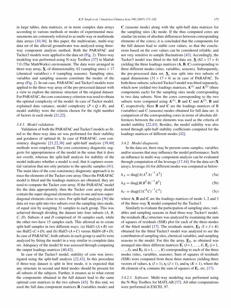
00% consistency, it could explain 50.47% of the total data vari-nce. The three components model on the other hand, althoughxplained 56.59% of variance, the core consistency droppedo 10.09%, thus showing its inadequacy to fit the data. Fig. 3hows the core consistency plot for two- and three-componentodel. It is evident that a simple two-component PARAFACodel explained sufficiently high variance (50.47%) of data

ariance. Some degree of non-tri-linearity in data may not allowARAFAC, a multi-linear model, to capture higher variance45]. Further, in order to see if the two-component PARAFACodel is valid and optimal in terms of complexity and stabil-

ty, the core consistency and split-half analysis diagnostics weresed [21,22,38]. If the PARAFAC model is valid then the coreonsistency is close to 100%. If the data cannot be approximatelyescribed by multi-linear model or too many components aresed the core consistency will be close to zero (or even nega-ive). A consistency value of around 50% indicates that models inappropriate [46]. In our case, although, the core consistencyalue for the two-component PARAFAC model was 100%, indi-ating that the model does not over fit the data, in split-halfnalysis, difference in loadings matrices in different modes wasbtained for two subsets. In case of multi-linear data structure,he split-half analysis should produce same scores for differentubsets. If same scores are not obtained, it could indicate dis-imilar interrelations in different subsets, hence non-linearties46]. Here, the split-half models were compared for similari-ies through computing the split-half stability coefficient [42].n our case, mean values of the split-half stability coefficientsor the two-component PARAFAC model were 0.91 and 1.26or sampling site mode (A), 0.03 and 0.04 for variables mode

B), and 0.03 and 0.21 for seasons mode (C). A value of theplit-half stability coefficient below 0.1 is considered indicatingufficiently stable model [42]. This implies that the model istable in variable mode, whereas, it is unstable in sampling site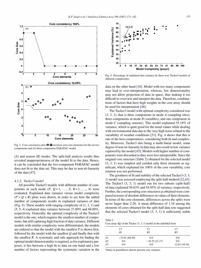

K.P. Singh et al. / Analytica Chimica Acta 596 (2007) 171–182 177

Fc

(rido

4

pe(n((rmnmaftopn

Fd

dmmdtb

(tmvwvoidcpo(nr

1ToFpIn terms of the core elements, differences across the splits werenever larger than 2.28. A mean difference of 1.16 among theelements of cores obtained for the split-half data sets suggestedthat the selected Tucker3 model (3, 3, 1) is sufficiently stable

Table 2Core array (G) of the Tucker (3, 3, 1) model in the unfolded form

C1 C1 C1B1 B2 B3

ig. 3. Core consistency plot ( / zero/non-zero core elements) for the (a) twoomponents and (b) three-components PARAFAC model.

A) and season (B) modes. The split-half analysis results thusevealed inappropriateness of the model fit to the data. Hence,t can be concluded that the two-component PARAFAC modeloes not fit to the data set. This may be due to non-tri-linearityf the data [47].

.1.2. Tucker3 modelAll possible Tucker3 models with different number of com-

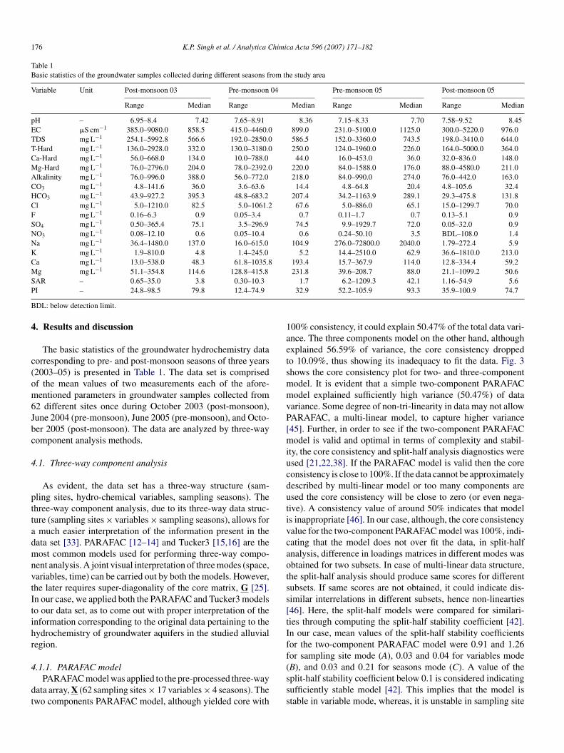
onents in each mode (P, Q = 1, . . ., 5; R = 1, . . ., 4) werevaluated. Explained data variance versus model complexityP × Q × R) plots were drawn, in order to see how the addedumber of components results in explained variance of dataFig. 4). These models with ranging complexity of (1, 1, 1) and5, 5, 4) explained data variance between 37.89% and 68.00%,espectively. Generally, the optimal complexity of the Tucker3odel is the one, which requires the smallest number of compo-

ents, but still capturing high fraction of data variance. Differentodels with similar complexity were differentiated, the models

re ordered so that the model with the smallest P is shown first,ollowed by the model with the smallest Q and finally that with

he smallest R. A systematic and safe approach for finding theptimal model dimensionality is required, as for exploratory pur-oses, it lies between a high fit to data on one hand and a lowumber of factors representing the systematic variation in the

AAA

V

ig. 4. Percentage of explained data variance by three-way Tucker3 models ofifferent complexities.

ata on the other hand [18]. Model with too many componentsay lead to over-interpretation, whereas, low dimensionalityay not allow projection of data in space, thus making it too

ifficult to overview and interpret the data. Therefore, combina-ions of factors that have high weights in the core array shoulde used for interpretation [48].

The Tucker3 model with optimal complexity considered was3, 3, 1), that is three components in mode A (sampling sites),hree components in mode B (variables), and one component inode C (sampling seasons). This model explained 55.18% of

ariance, which is quite good for the usual values while dealingith environmental data due to the very high noise related to theariability of weather conditions [31]. Fig. 4 shows that this isne of the best compromises, considering both fit and complex-ty. Moreover, Tucker3 also being a multi-linear model, someegree of non-tri-linearity in data may also result in low varianceaptured by the model [45]. Models with higher number of com-onents were discarded as they were less interpretable. Since theriginal core structure (Table 2) obtained for the selected model3, 3, 1) was simplest and yielded only three elements as sig-ificant, which explained for 100% of the core variability, coreotation was not performed.

The goodness of fit and stability of the selected Tucker3 (3, 3,) model was assessed employing the split-half method [22,43].he Tucker3 (3, 3, 1) model run for two subsets (split-half)f data explained 56.63% and 54.95% of variance, respectively.urther, the corresponding core structures as obtained were com-ared in terms of absolute differences in values of their elements.

1 −33.01 (68.49) 0.0 0.02 0.0 −18.35 (21.17) 0.03 0.0 0.0 12.83 (10.34)

alues in parentheses denote percent core variance.

178 K.P. Singh et al. / Analytica Chimica Acta 596 (2007) 171–182

Fb

[tosfa

(ssF7fittshib1dhfa3asKm

Fe

btG

tpnSifthe chemical composition of the groundwater. In general, thesevariables are of natural origin, emanating from soil weatheringprocesses, releasing ions from the aquifer matrix through dis-solution in to the groundwater. The region has predominance of

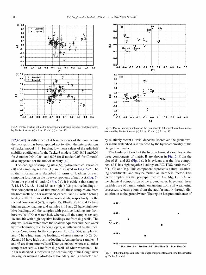
ig. 5. Plot of loading values for the components (sampling sites mode) extractedy Tucker3 model (a) A1 vs. A2 and (b) A1 vs. A3.

22,43,49]. A difference of 4.6 in elements of the core acrosshe two splits has been reported not to affect the interpretationsf Tucker model [43]. Further, low mean values of the split-halftability coefficients for the Tucker3 models (0.05, 0.04 and 0.04or A mode; 0.04, 0.04, and 0.08 for B mode; 0.05 for C mode)lso suggested for the model stability [42].

The loadings of sampling sites (A), hydro-chemical variablesB) and sampling seasons (C) are displayed in Figs. 5–7. Thepatial information is described in terms of loadings of eachampling location on the three components of matrix A (Fig. 5).rom the plot of A1 and A2 (Fig. 5a), it is evident that samples, 12, 17, 21, 43, 44 and 45 have high (>0.2) positive loadings inrst component (A1) of first mode. All these samples are from

he bore wells of Khar watershed, except 7 and 12, which belongo dug wells of Loni and Khar watersheds, respectively. In theecond component (A2), samples 15, 18–20, 30, 46 and 47 haveigh negative loadings and samples 9, 11 and 21 have high pos-tive loadings. All the samples with positive loadings are fromore wells of Khar watershed, whereas, all the samples (except8 and 46) with high negative loadings are from dug wells. Theug wells draw water from the shallow aquifers and their waterydro-chemistry, due to being open, is influenced by the localactors/conditions. In the component A3 (Fig. 5b), samples 43nd 45 have high negative loadings, whereas samples 10, 28, 30,2, and 37 have high positive loadings. Among these samples 43

nd 45 are from bore wells of Khar watershed, whereas all otheramples (except 37) are from dug wells of Khar watershed. Thehar watershed is located in the near vicinity of the Ganga riveraking its natural hydrological boundary and is characterized

Fb

ig. 6. Plot of loadings values for the components (chemical variables mode)xtracted by Tucker3 model (a) B1 vs. B2 and (b) B1 vs. B3.

y relatively recent alluvial deposits. Moreover, the groundwa-er in this watershed is influenced by the hydro-chemistry of theanga river water.The loadings of each of the hydro-chemical variables on the

hree components of matrix B are shown in Fig. 6. From thelot of B1 and B2 (Fig. 6a), it is evident that the first compo-ent (B1) has high negative loadings on EC, TDS, hardness, Cl,O4, Ca and Mg. This component represents natural weather-

ng constituents, and may be termed as ‘hardness’ factor. Thisactor emphasizes the principal role of Ca, Mg, Cl, SO4 on

ig. 7. Plot of loadings values for the single component (seasons mode) extractedy Tucker3 model.

himic

lfn(FhtosNnondftmttauttKab

tF2p

sio2tFseB

a(natp(HanA

iwnntaiwtccgwiKbwshpsts

(romptHoiac

ebaawOopcmTsrpnmi

K.P. Singh et al. / Analytica C

ime-stones, dolomite and calcareous shales and these accountor as much as 30% of the surface geology in the form of CaCO3odules, and Na- and K-carbonates [50]. The second componentB2) has high positive loadings on alkalinity, CO3, HCO3 and, which suggests that this component also represents generalydro-chemical variables and may be termed as ‘alkalinity’ fac-or. This factor also represents the natural geogenic variablesriginating from weathering and dissolution of the natural con-tituents of soil matrix. In the third component (B3), HCO3,O3, and K have high positive loadings, while F alone has highegative value (Fig. 6b). This factor may be considered as mixedne representing the anthropogenic species, such as NO3, origi-ated due to application of nitrogenous fertilizers and pH relatedissolution of fluoride bearing minerals in soil. It is supportedrom the results of earlier study [4], where the high mobility ofhe fluoride in the groundwater from the groundwater aquifer

atrix in the study area is reported. Moreover, the groundwa-er in the study area is mainly of sodium/potassium-bicarbonateype [4]. The dissolution of gases and minerals, particularly CO2nd CO3-related compounds in the atmosphere and in the unsat-rated zone during precipitation and infiltration, would imparthe observed HCO3 water type [51]. Further, feldspar is amonghe major minerals present in the region and kaolinization of-feldspar and consequent production of bicarbonate ions can

lso be explained by this factor. The geo-chemical reaction maye expressed [50] as:

2K-Feldspar + 2CO2 + 11H2O

= Kaolinite + 2K+ + 2HCO3− + 2H2SiO4

The loadings of the sampling seasons on the single (C1)emporal component (third mode) of matrix C are shown inig. 7. It is evident that both the post-monsoon seasons (2003,005) have relatively high positive loadings as compared to there-monsoon seasons (2004, 2005).

The core array, G of the model with dimensions, 62 (samplingites) × 17 (hydro-chemical variables) × 4 (sampling seasons),s displayed in Table 2. The core element gpqr reflects the extentf the interaction between Ap, Bq, and Cr (p = 1, 2, 3; q = 1,, 3; r = 1). It may be noted that in our case, there are onlyhree elements of relevance in the core, the ones for which p = q.urther, no core rotation was performed due to a simple coretructure obtained for the selected model. From Eq. (2), it isvident that the sign of gpqr is determined by the signs of Ap,q, and Cr.

Analysis of the core elements reveals that 100% of the vari-bility of the core is explained by the three elements, (1, 1, 1),2, 2, 1), and (3, 3, 1). The first core element (1, 1, 1) with aegative value (−33.01) explains 68.49% of the core variancend reflects the interactions between the first factors in each ofhe three modes (A1, B1, C1). Since all the loadings on sam-ling seasons mode (C1) are positive, sign of other two modesA1 and B1) determines the sign of first core element [16,21].

ence, this element can be explained through considering inter-

ctions between high positive loadings of A1 (Fig. 5a) and highegative loadings of B1 (hydro-chemical variables) (Fig. 6a).1 (first component of spatial mode) has high positive load-

op

w

a Acta 596 (2007) 171–182 179

ngs mainly on samples collected from bore wells of the Kharatershed and B1 (first component of variables mode) has highegative loadings on variables of natural origin (EC, TDS, hard-ess, Cl, SO4, Ca, Mg). Therefore, the first core element suggestshat groundwater samples (bore well) mainly of Khar watershedre dominated by the variables derived from natural weather-ng processes during both the pre- and post-monsoon seasonsith relatively larger influence during the later. It may be noted

hat A1 shows high positive loadings on groundwater samplesollected mainly from bore wells of Khar watershed. Since theonsidered water quality variables are mainly representing theeogenic processes in the study area and originating from naturaleathering (soil–water interactions) process, their dominance

n deeper groundwater aquifers is interpretable. Further, thehar watershed being closer to the Ganga river, is characterizedy relatively recent alluvial deposits which are more prone toeathering. Further, relatively higher loadings on post-monsoon

eason (Fig. 7) in mode C may be interpreted as a relativelyigh temperature during the summers enhances the weatheringrocesses manifold and the weathered species during the mon-oon are percolated down to the groundwater aquifers, impartingheir elevated levels as reflected in corresponding loadings ofubsequent post-monsoon seasons.

The second core element (2, 2, 1) with a negative value−18.35) explains 21.17% of the core variance (Table 2). Iteflects interactions between the second factors (A2 and B2)f first two modes (A and B) and the single factor of the thirdode (C). A2 has high negative loadings mainly on water sam-

les representing the dug wells of the study area (Fig. 5a). Onhe other hand, B2 has high positive loadings on alkalinity, CO3,CO3, and F (Fig. 6a). It suggests that the hydro-chemistryf groundwater belonging to the dug wells of the study areas dominated by variables derived from dissolution of carbon-tes yielding high alkalinity to water. It also reflects role of theation-exchange processes at the soil–water interface.

The third core element (3, 3, 1) with a positive sign (12.83)xplains 10.34% of the core variance. It reflects interactionsetween the third factors (A3 and B3) of first two modes (A and B)nd the single factor of third mode (C). A3 has positive and neg-tive loadings mainly on water samples collected from the dugells and bore wells, respectively, of the study region (Fig. 5b).n the other hand, B3 has high positive and negative loadingsn HCO3, NO3, K, and F, respectively (Fig. 6b). A joint inter-retation (A3, B3, C1) suggests that the bore well samples areontaminated with fluoride. High fluoride levels in groundwateray be attributed to its leaching from the soils in the region [4].he dug wells are relatively more contaminated with the speciesuch as nitrate released from the application of fertilizers in theegion during the post-monsoon season. The open dug wells arerone to such anthropogenic and local contamination. Domi-ance of these hydro-chemical species in post-monsoon wateray be understood, as high annual precipitation (about 850 cm)

n the region during the monsoon may enhance the dissolution

f weathered species from the sub-layers of the soil (aquifer)ercolating down to the deeper groundwater aquifers.

Further, in order to identify the hydro-chemical componentshich mainly contribute to the model and to evaluate the influ-

1 himic

etEptvavws(t3tpia

Fm

[samct(ehth(r

80 K.P. Singh et al. / Analytica C

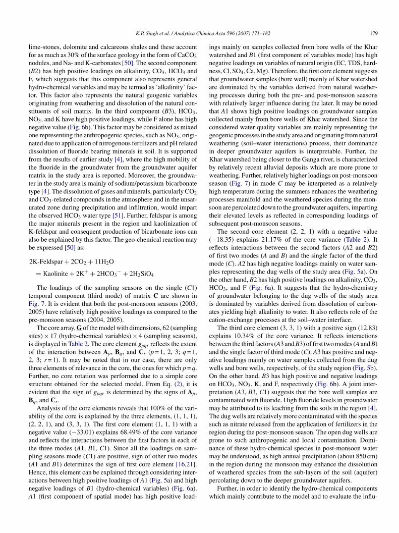
nce of spatial (sites) and temporal (sampling seasons) factors,he residuals matrix, Ex was analyzed. The residuals terms in

X arrays were squared and summed across the different modesroviding the residual sum-squared (SSR) variation as a func-ion of the corresponding mode, viz. sampling sites, chemicalariables and sampling seasons. A higher value of SSR for anttribute indicates its low contribution to the model and viceersa [17,23,44]. Further, the behaviour of the Tucker3 modelas studied in terms of leverage contribution for the first (hA),

econd (hB) and third (hC) modes corresponding to the spacesites), chemical variables and time (sampling seasons), respec-ively. Scattered plots of leverage versus SSR for mode 1, 2 andare presented in Fig. 8a–c. These plots can provide insight into

he extent of participation of a particular site, variable and sam-ling season in the model. Small SSR and high leverage valuendicate positive influence of an attribute, whereas higher SSRnd small leverage value for negative influence on the model

ig. 8. Leverage plotted against sum-squares of residuals (SSR) for (a) samplingode, (b) chemical variables mode, and (c) seasons mode.

sisth

ipfacmt(s

F(A

a Acta 596 (2007) 171–182

17,44]. The leverage versus SSR plot (Fig. 8a) for the first modehows that samples 21, 30, 43 and 45 have relatively higher lever-ge and low SSR values, thus showing positive influence on theodel. Relatively high values of SSR for samples 49 and 51 indi-

ate that these samples are not well fitted by the model. Amonghe variables, NO3 and F showed high leverage but low SSRFig. 8b), and hence both of these variables have positive influ-nce on the model. On the other hand, Na and EC, while havingighest SSR, exhibited moderate leverage showing their low par-icipation in the model. Further, among the seasons, relativelyigh leverage and low SSR for both the post-monsoon seasonsFig. 8c) revealed their high participation in the model, whereas,elatively high residuals (SSR) for the pre-monsoon (2005) sea-on shows that this season does not fit well in the model. Itndicates for some unusual hydro-geological event during thiseason influencing the groundwater quality in the region. Prioro the sampling time, there was an onset of rains, which couldave influenced the groundwater hydrochemistry in the region.

The Tucker3 model (3, 3, 1) was fitted to the data after remov-ng the outliers (samples 49 and 51; variables Na and EC; seasonre-monsoon 05) in all the three modes in a way similar to theull dataset. Model validation was performed through split-halfnalysis as earlier. The mean difference between the split-halfores elements was 1.15 with a maximum value of 2.23. Theodel captured almost the same variance (54.72%). The pat-

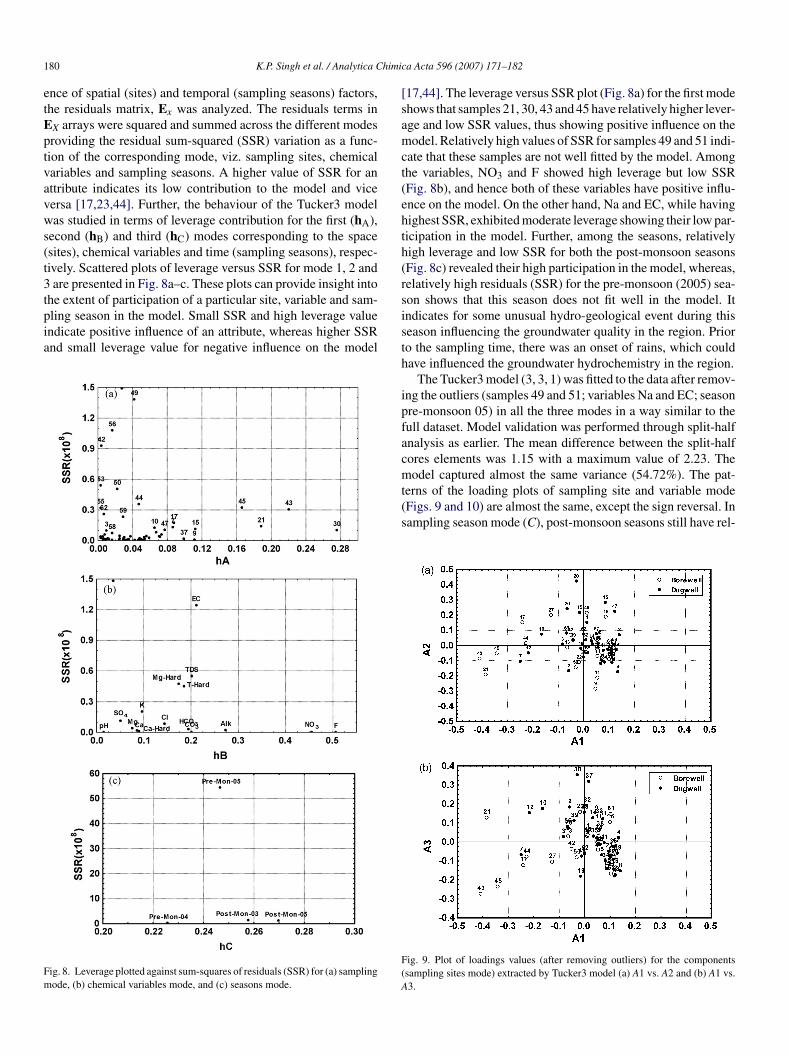
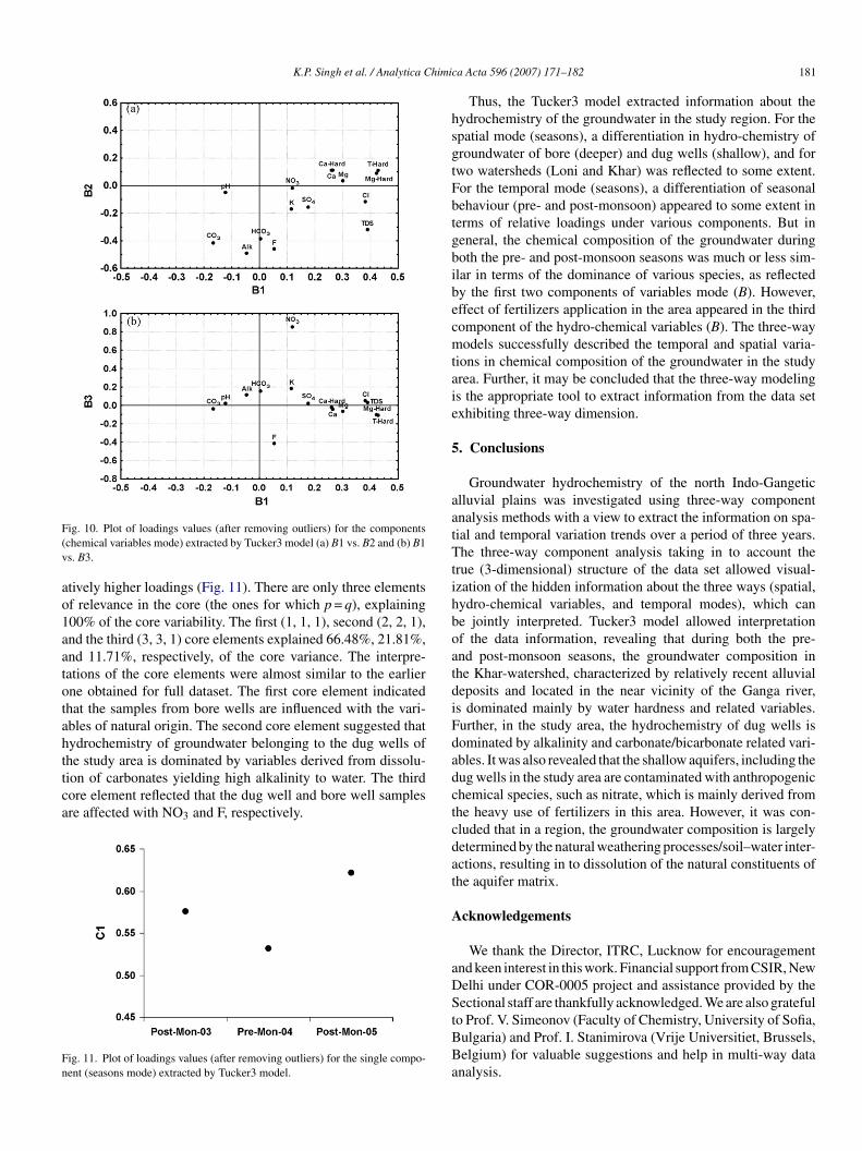
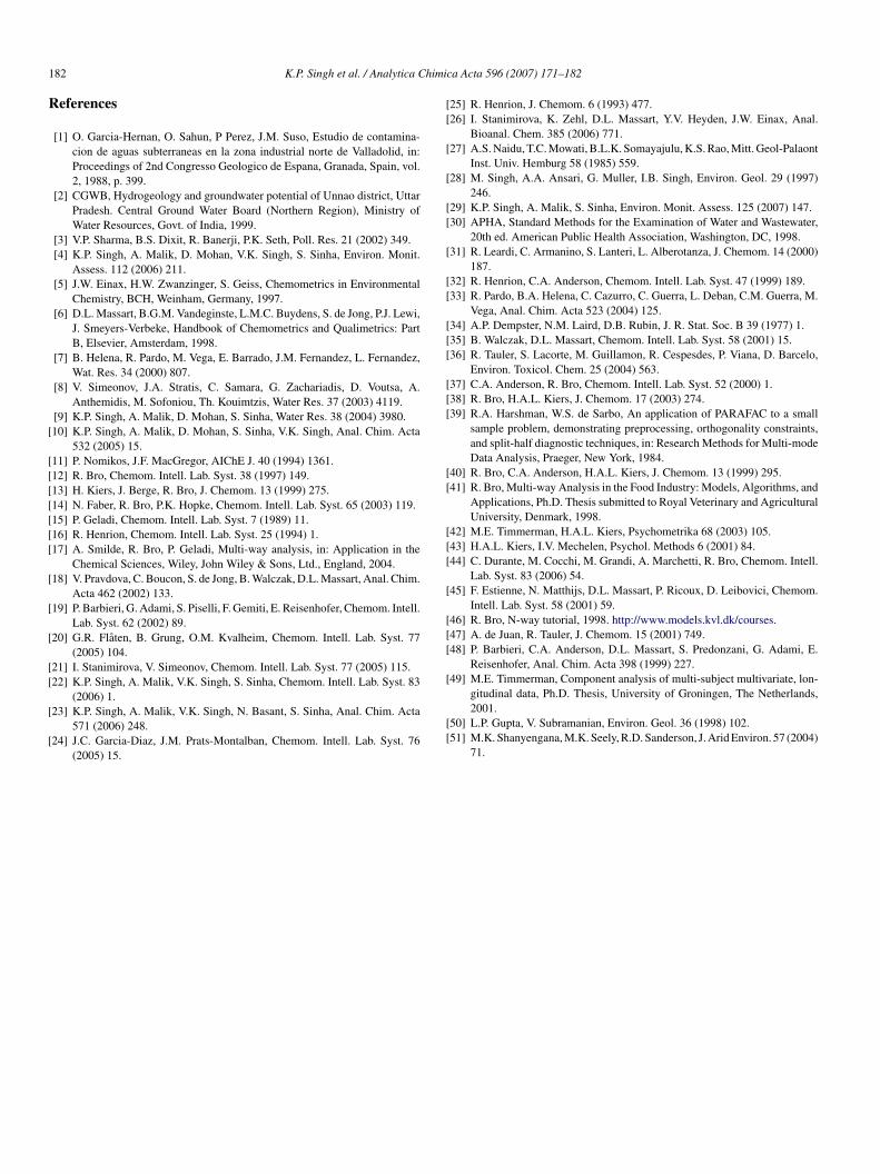
erns of the loading plots of sampling site and variable modeFigs. 9 and 10) are almost the same, except the sign reversal. Inampling season mode (C), post-monsoon seasons still have rel-

ig. 9. Plot of loadings values (after removing outliers) for the componentssampling sites mode) extracted by Tucker3 model (a) A1 vs. A2 and (b) A1 vs.3.

K.P. Singh et al. / Analytica Chimic

F(v

ao1aatotahttca

Fn

hsgtFbtgbibecmtaie

5

aatTtihboatdiFd

ig. 10. Plot of loadings values (after removing outliers) for the componentschemical variables mode) extracted by Tucker3 model (a) B1 vs. B2 and (b) B1s. B3.

tively higher loadings (Fig. 11). There are only three elementsf relevance in the core (the ones for which p = q), explaining00% of the core variability. The first (1, 1, 1), second (2, 2, 1),nd the third (3, 3, 1) core elements explained 66.48%, 21.81%,nd 11.71%, respectively, of the core variance. The interpre-ations of the core elements were almost similar to the earlierne obtained for full dataset. The first core element indicatedhat the samples from bore wells are influenced with the vari-bles of natural origin. The second core element suggested thatydrochemistry of groundwater belonging to the dug wells of

he study area is dominated by variables derived from dissolu-ion of carbonates yielding high alkalinity to water. The thirdore element reflected that the dug well and bore well samplesre affected with NO3 and F, respectively.

ig. 11. Plot of loadings values (after removing outliers) for the single compo-ent (seasons mode) extracted by Tucker3 model.

adctcdat

A

aDStBBa

a Acta 596 (2007) 171–182 181

Thus, the Tucker3 model extracted information about theydrochemistry of the groundwater in the study region. For thepatial mode (seasons), a differentiation in hydro-chemistry ofroundwater of bore (deeper) and dug wells (shallow), and forwo watersheds (Loni and Khar) was reflected to some extent.or the temporal mode (seasons), a differentiation of seasonalehaviour (pre- and post-monsoon) appeared to some extent inerms of relative loadings under various components. But ineneral, the chemical composition of the groundwater duringoth the pre- and post-monsoon seasons was much or less sim-lar in terms of the dominance of various species, as reflectedy the first two components of variables mode (B). However,ffect of fertilizers application in the area appeared in the thirdomponent of the hydro-chemical variables (B). The three-wayodels successfully described the temporal and spatial varia-

ions in chemical composition of the groundwater in the studyrea. Further, it may be concluded that the three-way modelings the appropriate tool to extract information from the data setxhibiting three-way dimension.

. Conclusions

Groundwater hydrochemistry of the north Indo-Gangeticlluvial plains was investigated using three-way componentnalysis methods with a view to extract the information on spa-ial and temporal variation trends over a period of three years.he three-way component analysis taking in to account the

rue (3-dimensional) structure of the data set allowed visual-zation of the hidden information about the three ways (spatial,ydro-chemical variables, and temporal modes), which cane jointly interpreted. Tucker3 model allowed interpretationf the data information, revealing that during both the pre-nd post-monsoon seasons, the groundwater composition inhe Khar-watershed, characterized by relatively recent alluvialeposits and located in the near vicinity of the Ganga river,s dominated mainly by water hardness and related variables.urther, in the study area, the hydrochemistry of dug wells isominated by alkalinity and carbonate/bicarbonate related vari-bles. It was also revealed that the shallow aquifers, including theug wells in the study area are contaminated with anthropogenichemical species, such as nitrate, which is mainly derived fromhe heavy use of fertilizers in this area. However, it was con-luded that in a region, the groundwater composition is largelyetermined by the natural weathering processes/soil–water inter-ctions, resulting in to dissolution of the natural constituents ofhe aquifer matrix.

cknowledgements

We thank the Director, ITRC, Lucknow for encouragementnd keen interest in this work. Financial support from CSIR, Newelhi under COR-0005 project and assistance provided by theectional staff are thankfully acknowledged. We are also grateful

o Prof. V. Simeonov (Faculty of Chemistry, University of Sofia,ulgaria) and Prof. I. Stanimirova (Vrije Universitiet, Brussels,elgium) for valuable suggestions and help in multi-way datanalysis.

1 himic

R

[

[[[[[[[

[

[

[

[[

[

[

[[

[

[

[[

[

[[

[[[

[[[

[[

[[[

[

[[[

[

82 K.P. Singh et al. / Analytica C

eferences

[1] O. Garcia-Hernan, O. Sahun, P Perez, J.M. Suso, Estudio de contamina-cion de aguas subterraneas en la zona industrial norte de Valladolid, in:Proceedings of 2nd Congresso Geologico de Espana, Granada, Spain, vol.2, 1988, p. 399.

[2] CGWB, Hydrogeology and groundwater potential of Unnao district, UttarPradesh. Central Ground Water Board (Northern Region), Ministry ofWater Resources, Govt. of India, 1999.

[3] V.P. Sharma, B.S. Dixit, R. Banerji, P.K. Seth, Poll. Res. 21 (2002) 349.[4] K.P. Singh, A. Malik, D. Mohan, V.K. Singh, S. Sinha, Environ. Monit.

Assess. 112 (2006) 211.[5] J.W. Einax, H.W. Zwanzinger, S. Geiss, Chemometrics in Environmental

Chemistry, BCH, Weinham, Germany, 1997.[6] D.L. Massart, B.G.M. Vandeginste, L.M.C. Buydens, S. de Jong, P.J. Lewi,

J. Smeyers-Verbeke, Handbook of Chemometrics and Qualimetrics: PartB, Elsevier, Amsterdam, 1998.

[7] B. Helena, R. Pardo, M. Vega, E. Barrado, J.M. Fernandez, L. Fernandez,Wat. Res. 34 (2000) 807.

[8] V. Simeonov, J.A. Stratis, C. Samara, G. Zachariadis, D. Voutsa, A.Anthemidis, M. Sofoniou, Th. Kouimtzis, Water Res. 37 (2003) 4119.

[9] K.P. Singh, A. Malik, D. Mohan, S. Sinha, Water Res. 38 (2004) 3980.10] K.P. Singh, A. Malik, D. Mohan, S. Sinha, V.K. Singh, Anal. Chim. Acta

532 (2005) 15.11] P. Nomikos, J.F. MacGregor, AIChE J. 40 (1994) 1361.12] R. Bro, Chemom. Intell. Lab. Syst. 38 (1997) 149.13] H. Kiers, J. Berge, R. Bro, J. Chemom. 13 (1999) 275.14] N. Faber, R. Bro, P.K. Hopke, Chemom. Intell. Lab. Syst. 65 (2003) 119.15] P. Geladi, Chemom. Intell. Lab. Syst. 7 (1989) 11.16] R. Henrion, Chemom. Intell. Lab. Syst. 25 (1994) 1.17] A. Smilde, R. Bro, P. Geladi, Multi-way analysis, in: Application in the

Chemical Sciences, Wiley, John Wiley & Sons, Ltd., England, 2004.18] V. Pravdova, C. Boucon, S. de Jong, B. Walczak, D.L. Massart, Anal. Chim.

Acta 462 (2002) 133.19] P. Barbieri, G. Adami, S. Piselli, F. Gemiti, E. Reisenhofer, Chemom. Intell.

Lab. Syst. 62 (2002) 89.20] G.R. Flaten, B. Grung, O.M. Kvalheim, Chemom. Intell. Lab. Syst. 77

(2005) 104.21] I. Stanimirova, V. Simeonov, Chemom. Intell. Lab. Syst. 77 (2005) 115.22] K.P. Singh, A. Malik, V.K. Singh, S. Sinha, Chemom. Intell. Lab. Syst. 83

(2006) 1.23] K.P. Singh, A. Malik, V.K. Singh, N. Basant, S. Sinha, Anal. Chim. Acta

571 (2006) 248.24] J.C. Garcia-Diaz, J.M. Prats-Montalban, Chemom. Intell. Lab. Syst. 76

(2005) 15.

[[

a Acta 596 (2007) 171–182

25] R. Henrion, J. Chemom. 6 (1993) 477.26] I. Stanimirova, K. Zehl, D.L. Massart, Y.V. Heyden, J.W. Einax, Anal.

Bioanal. Chem. 385 (2006) 771.27] A.S. Naidu, T.C. Mowati, B.L.K. Somayajulu, K.S. Rao, Mitt. Geol-Palaont

Inst. Univ. Hemburg 58 (1985) 559.28] M. Singh, A.A. Ansari, G. Muller, I.B. Singh, Environ. Geol. 29 (1997)

246.29] K.P. Singh, A. Malik, S. Sinha, Environ. Monit. Assess. 125 (2007) 147.30] APHA, Standard Methods for the Examination of Water and Wastewater,

20th ed. American Public Health Association, Washington, DC, 1998.31] R. Leardi, C. Armanino, S. Lanteri, L. Alberotanza, J. Chemom. 14 (2000)

187.32] R. Henrion, C.A. Anderson, Chemom. Intell. Lab. Syst. 47 (1999) 189.33] R. Pardo, B.A. Helena, C. Cazurro, C. Guerra, L. Deban, C.M. Guerra, M.

Vega, Anal. Chim. Acta 523 (2004) 125.34] A.P. Dempster, N.M. Laird, D.B. Rubin, J. R. Stat. Soc. B 39 (1977) 1.35] B. Walczak, D.L. Massart, Chemom. Intell. Lab. Syst. 58 (2001) 15.36] R. Tauler, S. Lacorte, M. Guillamon, R. Cespesdes, P. Viana, D. Barcelo,

Environ. Toxicol. Chem. 25 (2004) 563.37] C.A. Anderson, R. Bro, Chemom. Intell. Lab. Syst. 52 (2000) 1.38] R. Bro, H.A.L. Kiers, J. Chemom. 17 (2003) 274.39] R.A. Harshman, W.S. de Sarbo, An application of PARAFAC to a small

sample problem, demonstrating preprocessing, orthogonality constraints,and split-half diagnostic techniques, in: Research Methods for Multi-modeData Analysis, Praeger, New York, 1984.

40] R. Bro, C.A. Anderson, H.A.L. Kiers, J. Chemom. 13 (1999) 295.41] R. Bro, Multi-way Analysis in the Food Industry: Models, Algorithms, and

Applications, Ph.D. Thesis submitted to Royal Veterinary and AgriculturalUniversity, Denmark, 1998.

42] M.E. Timmerman, H.A.L. Kiers, Psychometrika 68 (2003) 105.43] H.A.L. Kiers, I.V. Mechelen, Psychol. Methods 6 (2001) 84.44] C. Durante, M. Cocchi, M. Grandi, A. Marchetti, R. Bro, Chemom. Intell.

Lab. Syst. 83 (2006) 54.45] F. Estienne, N. Matthijs, D.L. Massart, P. Ricoux, D. Leibovici, Chemom.

Intell. Lab. Syst. 58 (2001) 59.46] R. Bro, N-way tutorial, 1998. http://www.models.kvl.dk/courses.47] A. de Juan, R. Tauler, J. Chemom. 15 (2001) 749.48] P. Barbieri, C.A. Anderson, D.L. Massart, S. Predonzani, G. Adami, E.

Reisenhofer, Anal. Chim. Acta 398 (1999) 227.49] M.E. Timmerman, Component analysis of multi-subject multivariate, lon-

gitudinal data, Ph.D. Thesis, University of Groningen, The Netherlands,2001.

50] L.P. Gupta, V. Subramanian, Environ. Geol. 36 (1998) 102.51] M.K. Shanyengana, M.K. Seely, R.D. Sanderson, J. Arid Environ. 57 (2004)

71.