61

International Journal of Research in Advanced Engineering and Technology ISSN: 2455-0876; Impact Factor: RJIF 5.44 www.engineeringresearchjournal.com Volume 2; Issue 3; May 2016; Page No. 61-71

Sorting Techniques in data Structure Alluvial Zone

Monika Jain

Asst. Prof. Dayanand P.G. College, Hisar, Haryana, India.

Abstract Sorting is one of the major issues in computer science. Sorting is a technique to arrange the elements either in ascending or in descending order. There are a large number of methods to sort the elements. These all methods are basically divided into 2 categories: internal sorting & external sorting. Some of these methods need extra memory while others do not. These sorting techniques differ from each other on the basis of their time-space complexities, their stability and the methodology they approach. These may be used in linear as well as non-linear data structure. Keywords: Sorting, Bubble Sort, Selection Sort, Insertion Sort, Quick Sort, Merge Sort, Radix Sort, Tournament Sort, Topological Sort, Heap Sort, Complexity 1. Introduction Algorithm: it is a step by step procedure to represent a problem in a finite number of steps. Algorithms have a vital and key role in solving the computational problems. In computer science, an algorithm that puts elements of a list into a certain order is known as sorting algorithm. The orders that are mainly used are numerical order and lexicographical order. Sorting: It is a technique to rearrange the elements of a list either in ascending order or in descending order, which may be numerical, lexicographical or any other user defined order. Classification of sorting: Sorting is classified as: 1) Internal sorting 2) external sorting Internal Sorting: It is an applied when the entire collection of data is very small. It uses only primary memory during sorting process. No secondary memory is required. All the data that is to be sorted is accommodated at a time in the memory Types of internal sorting Selection sort-> example- selection sort algorithm, heap

sort algorithm. Insertion sort -> example- Insertion sort algorithm, shell

sort algorithm Exchange sort-> example- Bubble sort algorithm quick

sort algorithm Radix sort-> an example of distribution sort Topological sort is used in graphs External Sort: It is used to sort very large amount of data. It requires external or secondary memory like magnetic disk or tape to store the data because all the data is not fit into the primary memory. In this, read and write access time is considered. It is based on the process of merging. Example: merge sort

Bubble Sort: In this method, multiple exchanges take place in one pass. In this, 2 adjacent elements are compared and swapping is done if required. For the N number of elements in a list, (N-1) passes are required. Algorithm: Bubble_sort (A, N) Here A is an array with N elements. 1. Repeat steps 2 & 3 for I=1 to N-1 2. Set PTR:= 1 [Initialize pass pointer PTR] 3. Repeat while PTR < N-I : (execute pass) a) If A [PTR] > A [PTR+1] Then TEMP: = A [PTR] A [PTR]: = A [PTR+1] A [PTR+1]: = TEMP. [End of if] b) Set PTR: = PTR+1 [End of step 3 loop] [End of step 1 loop] 4 Exit. Complexity of bubble sort: F (n) = (n-1) + (n-2) + (n+3) -----3+2+1

=푛(푛 − 2)

2 = 푛2 −

푛2

= 0(n2)

Example: 32, 51, 27, 85, 66, 23, 13, 57, -8el Pass 1: i) a1 <a2 no change ii) a2 >a3 interchange elements

32, 27, 51, 85, 66, 23, 13, 57 iii) a3 < a4 no change iv) a4> a5 interchange elements

32, 27, 55, 66, 85, 23, 13, 57 v) a5 > a6 interchange elements

62

32, 27, 51, 66, 23, 85, 13, 57 vi) a6 > a7 interchange elements

32, 27, 51, 66, 23, 13, 85, 57 vii) a7 > a8 interchange elements

32, 27, 51, 66, 23, 13, 57, 85 At the end of pass 1, we found that the largest element is at last position and remaining elements are not sorted, so we proceed again. Pass 2: 32, 27, 51, 66, 23, 57, 85 i) a1 >a2 interchange elements

27, 32,51,66,23,13,57,85 ii) a2<a3 no change iii) a3<a4 no change iv) a4>a5 interchange elements

27, 32,51,23,66,13,57,85 v) a5>a6 interchange elements

27, 32,51,23,13,66,57,85 vi) a6>a7 interchange elements

27, 32,51,23,13,57,66,85

At the end of pass 2, second largest no 66 has moved to its position. Pass 3: 27, 32, 51, 23, 13, 57, 66, 85 i) a1<a2 no change ii) a2<a3 no change iii) a3<a4 inter change

27, 32,23,51,13,57,66,85 iv) a4>a5 inter change

27, 32,23,13,51,57,66,85 v) a5<a6 no change

3rd largest no 57 is at its position at the end of pass 3. 27, 32,23,13,51,57,66,85 Pass 4: 27, 32, 23, 13, 51, 57, 66, 85 i) a1< a2 no change ii) a2<a3 interchange elements

27, 23, 32, 13, 51, 57, 66, 85 iii) a3>a4 interchange elements

27, 23, 13, 32, 51, 57, 66, 85 iv) a4>a5 no change So a5, the 4th large no is at its original position at the end of pass-4. So list is 27, 23, 13, 32, 51, 57, 66, 85 Pass-5 i) a1>a2 interchange elements

23, 27, 13, 32, 57, 66, 85 ii) a2>a3 inter change elements

23, 13, 27, 32, 51, 57, 66, 85 iii) a3<a4 no change

23, 13, 27, 32, 51, 57, 66, 85 Pass-6 a1>a2 interchange elements 13, 23, 27, 32, 51, 57, 66, 85, a2<a3 no change

Pass-7: a1<a2 no change Thus 8 elements are sorted after 7 passes (actually after 6 passes) So, the sorted list is 13, 23, 27, 32, 51, 57, 66, 85. There may be cut down in the number of passes. So, if we

get the sorted list before n-1 passes for n elements, then we don’t need to continue.

Advantages: 1) Simplicity and ease of implementation. 2) Auxiliary Space used is O (1). Disadvantages: 1) Very inefficient. Selection Sort: Section sort is based on finding the smallest element in the list & place it at the first position, then the next smallest element is found and placed at 2nd position & so on until one element is left, it is also known as push down sort algorithm. Number of passes in selection sort is (n-1) if we have n elements. It is noted for its simplicity ever other algorithms in certain situations, particularly where the secondary memory is limited. Algorithm: Procedure MIN (A, K, N, LOC) A is an array. It is used to find the location LOC of smallest element among A [K], A[K+1]-----A[N] 1 Set MIN:= A [K] & LOC := K.[Initialize pointers] 2 Repeat for J = K+1 to N

If MIN > A [J] & LOC: = J then: Set MIN: = A [J] & LOC: =J [End of loop]

3 Return Algorithm: (Selection–sort) SELECTION (A, N) 1 Repeat steps 2 & 3 for K=1 to N-1 2 Call MIN (A, K, N, LOC) 3 [interchange A[K] & A[LOC]

Set TEMP: =A [K] A [K]:= A [LOC] A [LOC]:= TEMP

[End of step -1 loop] 4 Exit Complexity of selection sort algorithm: F(n) = (n-1) +(n-2)+ (n-3)---2+1 = ( )= O(n2) Advantages: 1) Simple and easy to implement. Disadvantages: 1) Inefficient for large lists, so similar to the more efficient

insertion sort, the insertion sort should be used in its place.

Example: An array with 8 elements 77, 33, 44, 11, 88, 22, 66, 35

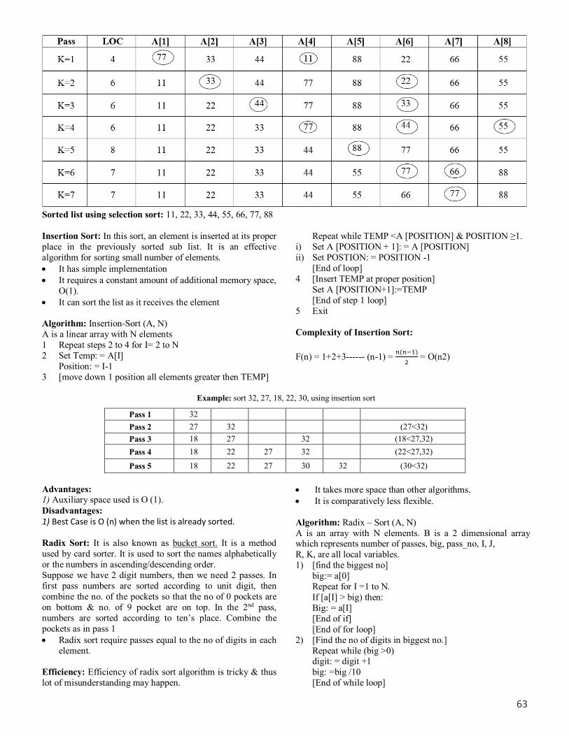
63

Sorted list using selection sort: 11, 22, 33, 44, 55, 66, 77, 88 Insertion Sort: In this sort, an element is inserted at its proper place in the previously sorted sub list. It is an effective algorithm for sorting small number of elements. It has simple implementation It requires a constant amount of additional memory space,

O(1). It can sort the list as it receives the element Algorithm: Insertion-Sort (A, N) A is a linear array with N elements 1 Repeat steps 2 to 4 for I= 2 to N 2 Set Temp: = A[I]

Position: = I-1 3 [move down 1 position all elements greater then TEMP]

Repeat while TEMP <A [POSITION] & POSITION ≥1. i) Set A [POSITION + 1]: = A [POSITION] ii) Set POSTION: = POSITION -1

[End of loop] 4 [Insert TEMP at proper position]

Set A [POSITION+1]:=TEMP [End of step 1 loop]

5 Exit Complexity of Insertion Sort: F(n) = 1+2+3------ (n-1) = ( )= O(n2)

Example: sort 32, 27, 18, 22, 30, using insertion sort

Pass 1 32 Pass 2 27 32 (27<32) Pass 3 18 27 32 (18<27,32) Pass 4 18 22 27 32 (22<27,32)

Pass 5 18 22 27 30 32 (30<32)

Advantages: 1) Auxiliary space used is O (1). Disadvantages: 1) Best Case is O (n) when the list is already sorted. Radix Sort: It is also known as bucket sort. It is a method used by card sorter. It is used to sort the names alphabetically or the numbers in ascending/descending order. Suppose we have 2 digit numbers, then we need 2 passes. In first pass numbers are sorted according to unit digit, then combine the no. of the pockets so that the no of 0 pockets are on bottom & no. of 9 pocket are on top. In the 2nd pass, numbers are sorted according to ten’s place. Combine the pockets as in pass 1 Radix sort require passes equal to the no of digits in each

element. Efficiency: Efficiency of radix sort algorithm is tricky & thus lot of misunderstanding may happen.

It takes more space than other algorithms. It is comparatively less flexible. Algorithm: Radix – Sort (A, N) A is an array with N elements. B is a 2 dimensional array which represents number of passes, big, pass_no, I, J, R, K, are all local variables. 1) [find the biggest no]

big:= a[0] Repeat for I =1 to N. If [a[I] > big) then: Big: = a[I] [End of if] [End of for loop]

2) [Find the no of digits in biggest no.] Repeat while (big >0) digit: = digit +1 big: =big /10 [End of while loop]

64

3) divisor:=1 4) repeat steps 5 to 8 for pass _no =0 to digit 5) [initialize the bucket count]

Repeat for K= 0 to 9 Count [K]:=0 [End of for loop]

6) [Perform the pass] Repeat for I = 0 to N-1 R: = (a[I]/divisor) mod 10 B[r] [count [r] +1]:=a[i] [End of loop]

7) [Collect elements from bucket} I:=0 Repeat for K= 0 to 9 Repeat for I=0 to count[K] A[I+1]=: = b[K] [J] [end of I loop] [end of K loop]

8) divisor : = divisor * 10 [end of step3 loop]

9) [finished] exit. Complexity of Radix Sort: No of comparisons to sort n elements of m digits each is C< n *m * 10 In worst case, n=m, So, C= o (n2) In best case, m = log2 n, So, C= o (n log n) Example: let we have 6 no with 3 digits 342, 98, 514, 428, 321, 134 Pass 1: sort according to unit place

Unit place 0 1 2 3 4 5 6 7 8 9 Numbers - 321 342 - 514 - 986 - 428 -

134 Pass 2: Sort according to ten’s place

0 1 2 3 4 5 6 7 8 9 - 514 321 134 342 - - - 986 - 428 134

Pass 3: Now sort according to hundred’s place

0 1 2 3 4 5 6 7 8 9 - 134 - 321 428 514 - - - 986 342

So sorted list is 134, 321, 342, 428, 514, 986 Algorithm: (2nd method)

[Initialization] Large = largest element in the array num = total no of digits is the largest element Digit = num Pass = 1

1. Repeat steps 3 to 8 while pass < nun 2. Initialize bucket & set i = 0 3. Repeat steps 5 to 7 while i < n-1

4. Set k = pass-1 (Position of A[i]) 5. Put A [i] into bucket k. 6. Set i: = i + 1 7. Set pass: = pass + 1 8. Print the numbers from bucket 9. Exit Quick Sort: It is a divide & conquers method introduced by Hoare in 1962. It is a very fast internal sorting technique. First divide the problem into sub lists. It is also known as

partition exchange sort Eg:

Starting from right, visit every element from right to left & compare it with leftmost element i.e. 44 & if number is found less than 44, replace it with 44

Starting from left, visit every element from L to R & compare with 44. If no found is greater than 44, replace them.

Starting from right, visit every element From R to I & compare with 44 & no found less than 44, then replace

Starting from left visit every element From L to R & compare every el with 44 & if found greater than 44, then exchange.

Now we see & compare from R to L, no number is less than 44 in between 44 & 77. So 44 is at its position. The List is divided into 2 Sub lists Sub list 1. [22, 33, 11, 40] 44 exact loc. Sub list 2. [90, 77, 60, 99, 55, 88, 66] Lower bounds of sub list 1 & 2 are 1 & 6 resp. Upper bounds of sub list 1 & 2 are 4 & 12 resp. Now, we will precede the same again & again a no of times till both the sub lists become sorted. Every time the sub list is again divided into 2 sub lists. At last, we obtain the sorted list. Complexity of Quick Sort In, average case, no of comparisons = O(n log2 n) In worst case, no of comparisons = O(n2) Working procedure 1. Choose the first element. 2. Rearrange the list such that first element will be at its

accurate position in list. Elements with lesser values are

65

the preceding elements & element with larger values are the succeeding elements.

3. Now we get 2 sub lists & 1 sorted element 4. Repeat steps 1-3 for all the sub lists until we get a sorted

list.

Procedure: Quick (A, N, BEG, END, LOC) 1 Set LEFT: =BEG & RIGHT: = END & LOC: = BEG. 2 Scan from right to left a) Repeat while A [LOC] < A [RIGHT] & LOC ≠ RIGHT.

RIGHT: = RIGHT-1 b) If LOC : = RIGHT then return c) If A [LOC] > A[Right] i) (Inter change A [LOC] & A[RIGHT])

TEMP: = A [LOC] A [LOC]: = A [RIGHT]

A [RIGHT]: = TEMP. ii) Set LOC : = RIGHT iii) GOTO step 3 3. (a) Repeat while A[LEFT] < A[LOC] & LEFT≠LOC

(a) LEFT: = LEFT +1 (b) If LOC: = LEFT then return (c) If A [LEFT] > A [LOC] then (i) [Interchange elements] TEMP: = A [LOC]

A[LOC]: =A[LEFT] A[LEFT]: = TEMP

(ii) set LOC : = LEFT (iii) GOTO step 2.

4. Return Algorithm for quick sort 1. [Initialize] TOP: = NULL. 2. [Push boundary values of A onto stock when A has 2 or more elements] If N>1 then: = TOP: = TOP+1

LOWER [1]: = 1 UPPER [1]:=N

3. Repeat steps 4 to 7 while TOP ≠ NULL 4. [Pop sub list from stack] Set BEG: = LOWER [TOP] END: = UPPER [TOP] Top: = Top-1 5. Call quick (A, N, BEG, END, LOC) 6. [Push left sub list onto stack when it has 2 or more elements] If BEG<LOC-1 then: Top: =Top+1 LOWER [TOP]: =BEG Upper [Top]: = LOC-1 [End of if structure] 7. [Push right sub list onto stack when it has = or more elements] If LOC+1< END then: TOP: = TOP+1 LOWER [TOP]: = LOC+1 UPPER [TOP]: =END [End of if structure] [End of step 3 loop] 8. Exit.

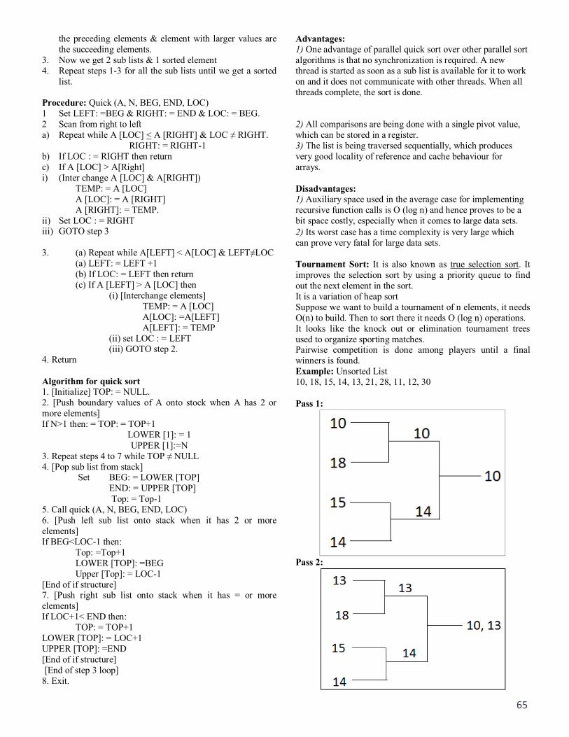
Advantages: 1) One advantage of parallel quick sort over other parallel sort algorithms is that no synchronization is required. A new thread is started as soon as a sub list is available for it to work on and it does not communicate with other threads. When all threads complete, the sort is done. 2) All comparisons are being done with a single pivot value, which can be stored in a register. 3) The list is being traversed sequentially, which produces very good locality of reference and cache behaviour for arrays. Disadvantages: 1) Auxiliary space used in the average case for implementing recursive function calls is O (log n) and hence proves to be a bit space costly, especially when it comes to large data sets. 2) Its worst case has a time complexity is very large which can prove very fatal for large data sets. Tournament Sort: It is also known as true selection sort. It improves the selection sort by using a priority queue to find out the next element in the sort. It is a variation of heap sort Suppose we want to build a tournament of n elements, it needs O(n) to build. Then to sort there it needs O (log n) operations. It looks like the knock out or elimination tournament trees used to organize sporting matches. Pairwise competition is done among players until a final winners is found. Example: Unsorted List 10, 18, 15, 14, 13, 21, 28, 11, 12, 30

Pass 1:

Pass 2:

66

Pass 3:

Pass 4:

Pass 5:

Now if we put 11 in the sequence, the sorted sequence will be broken. Hence we have to disqualify the element by putting * mark on it. Element is disqualified if key (new)< key(last out) So Pass 5:

Pass 6:

12 is disqualified So

Pass 7:

Pass 8:

Pass 9: Make a separate list of the disqualified elements, we get

Pass 10: We have 2 sorted lists: i) 10, 13, 14, 15, 18, 21, 28, 30 ii) 11, 12 Now, merge both the sub lists to get a sorted list 10,11,12,13,14,15,18,21,28,30 Complexity: Worst case – O (n log n) Average case- O (n log n) Merge Sort: It is based on divide & conquer strategy First we divide the list into 2 sub lists (divide) Each half is sorted independently (conquer) Then these 2 sorted halves are merged to give a sorted list

It has 3 phases:

1. Divide 2. Conquer 3. Combine Problem is

divided into sub problems

Sub problems are solved

Solution of sub problems are recombined to give the solution

of original problem Complexity No of comparisons = n-1 = O (n) No of merges = O(log n) So Complexity of merge sort= O (n logn) It requires large storage So complexity for worst case= O (n logn)

67

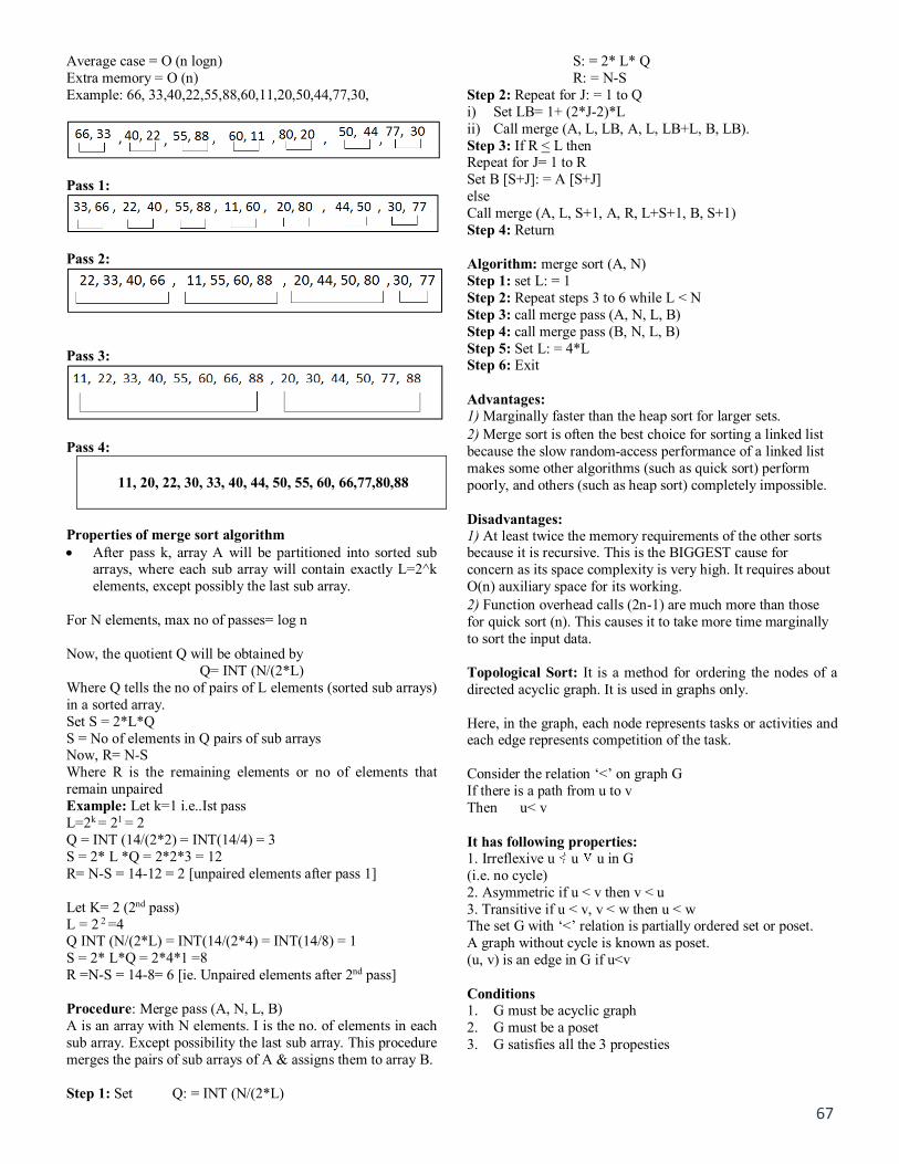
Average case = O (n logn) Extra memory = O (n) Example: 66, 33,40,22,55,88,60,11,20,50,44,77,30,

Pass 1:

Pass 2:

Pass 3:

Pass 4:

11, 20, 22, 30, 33, 40, 44, 50, 55, 60, 66,77,80,88

Properties of merge sort algorithm After pass k, array A will be partitioned into sorted sub

arrays, where each sub array will contain exactly L=2^k elements, except possibly the last sub array.

For N elements, max no of passes= log n Now, the quotient Q will be obtained by

Q= INT (N/(2*L) Where Q tells the no of pairs of L elements (sorted sub arrays) in a sorted array. Set S = 2*L*Q S = No of elements in Q pairs of sub arrays Now, R= N-S Where R is the remaining elements or no of elements that remain unpaired Example: Let k=1 i.e..Ist pass L=2k = 21 = 2 Q = INT (14/(2*2) = INT(14/4) = 3 S = 2* L *Q = 2*2*3 = 12 R= N-S = 14-12 = 2 [unpaired elements after pass 1] Let K= 2 (2nd pass) L = 2 2 =4 Q INT (N/(2*L) = INT(14/(2*4) = INT(14/8) = 1 S = 2* L*Q = 2*4*1 =8 R =N-S = 14-8= 6 [ie. Unpaired elements after 2nd pass] Procedure: Merge pass (A, N, L, B) A is an array with N elements. I is the no. of elements in each sub array. Except possibility the last sub array. This procedure merges the pairs of sub arrays of A & assigns them to array B. Step 1: Set Q: = INT (N/(2*L)

S: = 2* L* Q R: = N-S

Step 2: Repeat for J: = 1 to Q i) Set LB= 1+ (2*J-2)*L ii) Call merge (A, L, LB, A, L, LB+L, B, LB). Step 3: If R < L then Repeat for J= 1 to R Set B [S+J]: = A [S+J] else Call merge (A, L, S+1, A, R, L+S+1, B, S+1) Step 4: Return Algorithm: merge sort (A, N) Step 1: set L: = 1 Step 2: Repeat steps 3 to 6 while L < N Step 3: call merge pass (A, N, L, B) Step 4: call merge pass (B, N, L, B) Step 5: Set L: = 4*L Step 6: Exit Advantages: 1) Marginally faster than the heap sort for larger sets. 2) Merge sort is often the best choice for sorting a linked list because the slow random-access performance of a linked list makes some other algorithms (such as quick sort) perform poorly, and others (such as heap sort) completely impossible. Disadvantages: 1) At least twice the memory requirements of the other sorts because it is recursive. This is the BIGGEST cause for concern as its space complexity is very high. It requires about O(n) auxiliary space for its working. 2) Function overhead calls (2n-1) are much more than those for quick sort (n). This causes it to take more time marginally to sort the input data. Topological Sort: It is a method for ordering the nodes of a directed acyclic graph. It is used in graphs only. Here, in the graph, each node represents tasks or activities and each edge represents competition of the task. Consider the relation ‘<’ on graph G If there is a path from u to v Then u< v It has following properties: 1. Irreflexive u u u in G (i.e. no cycle) 2. Asymmetric if u < v then v < u 3. Transitive if u < v, v < w then u < w The set G with ‘<’ relation is partially ordered set or poset. A graph without cycle is known as poset. (u, v) is an edge in G if u<v Conditions 1. G must be acyclic graph 2. G must be a poset 3. G satisfies all the 3 propesties

68

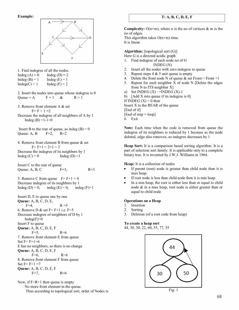
Example:

1. Find indegree of all the nodes. Indeg (A) = 0 Indeg (D) = 2 Indeg (B) = 1 Indeg (E) = 1 Indeg(C) = 1 Indeg (F) = 2 2. Insert the nodes into queue whose indegree is 0 Queue = A F = 1 & R = 1 3. Remove front element A & set

F= F + 1 =2 Decrease the indegree of all neighbors of A by 1

Indeg (B) =1-1=0 Insert B to the rear of queue, as indeg (B) = 0 Queue: A, B F=2, R=2 4. Remove front element B from queue & set

F= F+1 = 2+1 = 3 Decrease the indegree of its neighbors by 1 Indeg (C) = 0 Indeg (D) =1 Insert C to the rear of queue Queue: A, B, C F=3, R=3 5. Remove C from queue F= F+1 = 4 Decrease indegree of its neighbors by 1 Indeg (D) = 0, indeg (E) = 0, indeg (F)=1 Insert D, E to queue one by one Queue: A, B, C, D, E,

F=4, R =5 6. Remove D & set F= F+1 i.e. F=5 Decrease indegree of neighbors of D by 1

Indeg(F)=0 Insert F to queue Queue: A, B, C, D, E, F

F=5, R=6 7. Remove front element E from queue Set F= F+1=6 E has no neighbors, so there is no change Queue: A, B, C, D, E, F

F=6, R=6 8. Remove front element F from queue Set F= F+1 =7 Queue: A, B, C, D, E, F

F=7, R=6 Now, if F=R+1 then queue is empty

No more front element in the queue. Thus according to topological sort, order of Nodes is

T: A, B, C, D, E, F

Complexity: O(n+m), where n is the no of vertices & m is the no of edges. This algorithm takes O(n+m) time. It is linear Algorithm: [topological sort (G)] Here G is a directed acidic graph 1. Find indegree of each node no of G

INDEG (N) 2. Insert all the nodes with zero indegree to queue 3. Repeat steps 4 & 5 unit queue is empty 4. Delete the front node N of queue & set Front:= Front +1 5. Repeat for each neighbor X of node N [Delete the edges

from N to ITS neighbor X] a) Set INDEG (X) : =INDEG (X)-1 b) [Add X into queue if its indegree is 0] If INDEG (X) = 0 then Insert X to the REAR of the queue [End of if] [End of step = loop] 6. Exit Note: Each time when the code is removed from queue the indegree of its neighbors is reduced by 1 because as the node deleted, edge also removes, so indegree decreases by 1 Heap Sort: It is a comparison based sorting algorithm. It is a part of selection sort family. It is applicable only to a complete binary tree. It is invented by J.W.J. Williams in 1964. Heap: It is a collection of nodes If parent (root) node is greater than child node then it is

max heap. If root node is less than child node then it is min heap. In a min heap, the root is either less than or equal to child

node & in a max heap, root node is either greater than or equal to child node

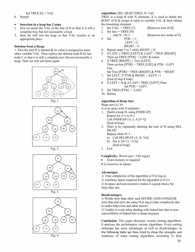
Operations on a Heap 1. Insertion 2. Sorting 3. Deletion (of a root code from heap) To create a heap sort 44, 30, 50, 22, 60, 55, 77, 55

Fig: 1

69

Fig: 2

Fig: 3

Fig: 4

Fig: 5

Fig: 6

Fig: 7

Fig: 8

Fig: 9

Insertion in a Heap: It is used to insert an element in a heap tree. Algorithm (INSHEAP (TREE, N, VAL) VAL is the value to be inserted. N is the no of nodes in a heap tree. 1. [Add new node to it & initialize PTR]

Set N: =N+1 & PTR: = N 2. [Find location to insert VAL].

Repeat steps 3 to 6 while PTR <1 3. Set PAR: = └PTR/2˩ (Greatest Integer Function) 4. If VAL < TREE [PAR] then

Set TREE [PTR]: = VAL & return. 5. Set TREE [PTR]: = TREE [PAR] [Moves node down] 6. Set PTR: = PAR [update PTR] 7. [Assign VAL as root of H]

70

Set TREE [I]: = VAL 8. Return Insertion in a heap has 2 steps 1. first we insert the VAL at the end of H so that it is still a

complete tree, but not necessarily a heap 2. then we will sort the heap so that VAL reaches to its

appropriate place Deletion from a Heap: 1. First the root R is deleted & its value is assigned to some other variable VAL. Then replace the deleted node R by last node L so that it is still a complete tree, but not necessarily a heap. Then we will sort them again

Fig: 1

Fig: 2

Fig: 3

Fig: 4

Algorithm: DEL HEAP (TREE, N, Val) TREE is a heap H with N elements. It is used to delete the ROOT of H & assign it value to variable VAL & then reheap the remaining elements. 1. Set VAL: = TREE [1] [Removes root of H] 2. Set last := TREE [N]

And N: =N-1 [Removes last mode of N] 3. Set PTR: = 1,

LEFT: =2, RIGHT: =3

4. Repeat steps 5 to 7 while RIGHT < N 5. If LAST ≥ TREE [LEFT] & LAST > TREE [RIGHT]

Then set TREE [PTR]: = LAST & return 6. If TREE [RIGHT] < Tree [LEFT]

Then set tree [PTR]: = TREE [LEF] & PTR: =LEFT Else Set Tree [PTR]:= TREE [RIGHT] & PTR: = RIGHT

7. Set LEFT: 2* PTR & RIGHT : =LEFT +1 [End of step 4 loop]

8. If LEFT = N & if LAST< TREE [LEFT] Then Set PTR: = LEFT

9. Set TREE [PTR] : = LAST 10. Return Algorithm of Heap Sort Heap sort (A, N) A is an array with N elements 1. [build a heap H, using INSHEAP]

Repeat for J=1 to N-1 Call INSHEAP (A, J, A [J+1]) [End of loop]

2. [Sort A by repeatedly deleting the root of H using DEL HEAP] Repeat while N>1 a) Call DELHEAP (A, N, Val) b) Set A [N+1] :=VAL

[End of loop] 3. Exit Complexity: Worst case = O(n log2n) Extra memory is required It is recursive in nature. Advantages: 1) Time complexity of the algorithm is O (n log n). 2) Auxiliary Space required for the algorithm is O (1). 3) In-space and non-recursive makes it a good choice for large data sets. Disadvantages: 1) Works slow than other such DIVIDE-AND-CONQUER sorts that also have the same O (n log n) time complexity due to cache behaviour and other factors. 2) Unable to work when dealing with linked lists due to non-convertibility of linked lists to heap structure. Conclusion: This paper discusses various sorting algorithms. It analyses the performance various algorithms. Every sorting technique has some advantages as well as disadvantages. In the following table we have tried to show the strengths and weakness of some sorting algorithms according to their

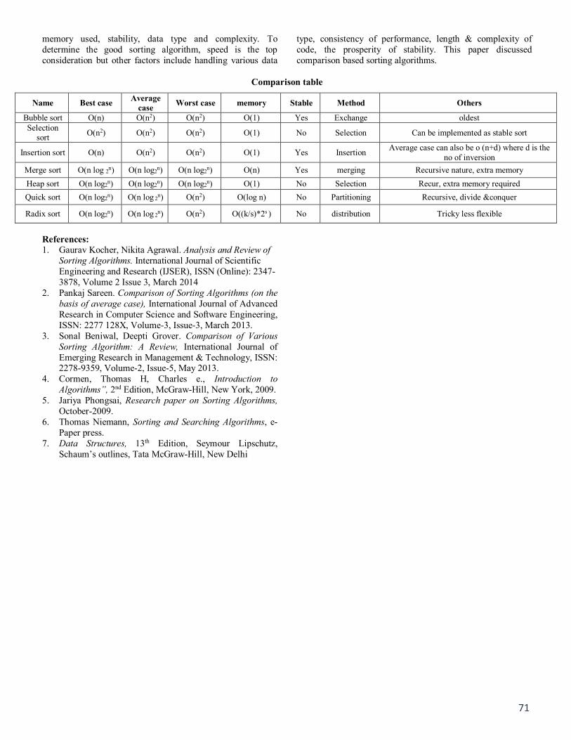
71

memory used, stability, data type and complexity. To determine the good sorting algorithm, speed is the top consideration but other factors include handling various data

type, consistency of performance, length & complexity of code, the prosperity of stability. This paper discussed comparison based sorting algorithms.

Comparison table

Name Best case Average case Worst case memory Stable Method Others

Bubble sort O(n) O(n2) O(n2) O(1) Yes Exchange oldest Selection

sort O(n2) O(n2) O(n2) O(1) No Selection Can be implemented as stable sort

Insertion sort O(n) O(n2) O(n2) O(1) Yes Insertion Average case can also be o (n+d) where d is the no of inversion

Merge sort O(n log 2n) O(n log2n) O(n log2n) O(n) Yes merging Recursive nature, extra memory Heap sort O(n log2n) O(n log2n) O(n log2n) O(1) No Selection Recur, extra memory required Quick sort O(n log2n) O(n log 2n) O(n2) O(log n) No Partitioning Recursive, divide &conquer

Radix sort O(n log2n) O(n log 2n) O(n2) O((k/s)*2s ) No distribution Tricky less flexible

References: 1. Gaurav Kocher, Nikita Agrawal. Analysis and Review of

Sorting Algorithms. International Journal of Scientific Engineering and Research (IJSER), ISSN (Online): 2347-3878, Volume 2 Issue 3, March 2014

2. Pankaj Sareen. Comparison of Sorting Algorithms (on the basis of average case), International Journal of Advanced Research in Computer Science and Software Engineering, ISSN: 2277 128X, Volume-3, Issue-3, March 2013.

3. Sonal Beniwal, Deepti Grover. Comparison of Various Sorting Algorithm: A Review, International Journal of Emerging Research in Management & Technology, ISSN: 2278-9359, Volume-2, Issue-5, May 2013.

4. Cormen, Thomas H, Charles e., Introduction to Algorithms”, 2nd Edition, McGraw-Hill, New York, 2009.

5. Jariya Phongsai, Research paper on Sorting Algorithms, October-2009.

6. Thomas Niemann, Sorting and Searching Algorithms, e-Paper press.

7. Data Structures, 13th Edition, Seymour Lipschutz, Schaum’s outlines, Tata McGraw-Hill, New Delhi