CHARACTERIZATION OF THE HYDROGEOLOGY OF THE LODWAR ALLUVIAL

AQUIFER SYSTEM, TURKANA COUNTY, KENYA

BY;

FLORENCE JEROTICH TANUI

I80/51693/2017

A THESIS SUBMITTED IN FULFILLMENT OF THE REQUIREMENTS FOR THE AWARD

OF THE DEGREE OF DOCTOR OF PHILOSOPHY IN GEOLOGY OF THE UNIVERSITY

OF NAIROBI

2021

ii

DECLARATION

I declare that this thesis is my original work and has not been submitted elsewhere for examination,

award of degree or publication. Where other people’s work or my own work has been used, this

has been properly acknowledged and referenced in accordance with the University of Nairobi’s

requirements.

Signature…………………………………… Date…………………………………….....……

Florence Jerotich Tanui

I80/51693/2017

Department Earth and Climate Sciences

University of Nairobi

This thesis is submitted for examination with our approval as research supervisors:

Prof Daniel Olago Signature………… …………………Date………….……………...

Department of Earth and Climate Sciences

University of Nairobi

P.O box 30197-00100

Nairobi Kenya

Dr Gilbert Ouma Signature……………………………Date………….……………...

Department of Earth and Climate Sciences

University of Nairobi

P.O box 30197-00100

Nairobi Kenya

Dr Zachariah Kuria Signature…………….................…Date………….……………...

Department of Earth and Climate Sciences

University of Nairobi

P.O box 30197-00100

Nairobi Kenya

December 03, 2021

December 03, 2021

December 03, 2021

December 03, 2021

iii

DEDICATION

I dedicate this research to my family. A special feeling and gratitude to my loving parents, my

mother Alice for your prayers and to my late father William Rutto for the unique inspiration to my

hard work and to all my siblings for being incredible cheerleaders throughout the entire doctorate

program. Special dedication to my loving husband, who encouraged me to pursue my dreams and

finish my thesis, and to my son and daughter for being the constant source of joy. Finally, to the

Almighty God for good health throughout the study period.

iv

ACKNOWLEDGEMENTS

The REACH Program, funded by UK Aid from the UK Foreign, Commonwealth and

Development Office (FCDO) for the benefit of developing countries, provided funding for this

study (Program Code 201880), covering tuition fees, data collection and analysis, and a monthly

stipend. However, the opinions expressed and the information provided therein are not necessarily

those endorsed by the FCDO, which cannot accept any liability for or reliance on such views or

information.

I acknowledge the members of the REACH programme in all the partner countries, Kenya,

Ethiopia, Bangladesh and the University of Oxford, who inspired the new research dimension

related to water security. My appreciation goes to the REACH Kenya fraternity for the invaluable

support in logistics and assistance during the data collection. The writing of this thesis would not

have been successful without the invaluable support of my University Supervisors for technical

guidance and exemplary supervision, especially Prof Daniel Olago, who was my lead supervisor.

Special thanks go to my family for your constant support and motivation, especially for allowing

me to go for my fieldworks, conferences, and workshops pertaining to my studies. I will forever

be grateful for all your prayers throughout my study period.

v

ABSTRACT

Drylands account for more than a third of the world's land area and are characterized by less than

250 mm of rainfall per year. In these regions, groundwater is a strategic resource and plays a key

role in economic development, especially in sub-Saharan Africa, where it is responsible for

improving livelihoods. Lodwar town depends primarily on a poorly studied groundwater system

for its municipal water supplies. The aim of this research was to establish the sustainability of this

aquifer system through a comprehensive study of its hydrogeological characteristics, sensitivity to

climate variability, and the influence of natural and anthropogenic processes, all of which are

currently unknown yet critical for its sustainable management. The methods used were: detailed

geological mapping and rock analysis (petrography and X-ray fluorescence); remote sensing

(digital elevation models and vegetation cover maps) and drone mapping of Lodwar town for

stream lineament analysis; evaluation of borehole drilling datasets including yields, static water

levels, water rest levels, drawdowns, transmissivities, and borehole depth; geophysical surveys

involving vertical electrical soundings for evaluation of the hydrogeological characteristics;

aquifer hydrogeochemistry of surface (river, scoop holes, water pans) and groundwater, where

field measurements included pH, Temp, and EC using hand-held Combo Tester HI98129 while,

turbidity, total hardness, alkalinity, Ca2+, Mg2+, Na, K+, Fe2+, Mn2+, Cl-, F-, HCO3-, SO4

2- and CO32-

NO3-, NO2

- were measured at the Water Resources Central Laboratory based standard analytical

procedures. Furthermore, stable isotopic analyses of oxygen-18, deuterium and tritium in water

samples was done at Elemtex Lab, United Kingdom to establish the rainfall-surface water-

groundwater interactions, groundwater age and recharge sources. The multifaceted dataset was

analysed using descriptive and inferential statistics, including principal component analysis

(PCA), hierarchical cluster analysis (HCA), the software PHREEQC for analysis of the water

chemistry data, and all together, to develop the first conceptual aquifer model for this system. The

findings of this research revealed that Lodwar and its surroundings are underpinned by three

different and interconnected freshwater (<1000µS/cm) aquifers (shallow alluvial aquifer (SAA),

the intermediate aquifer (IA) and the deep aquifer (DA)) that are collectively referred to as the

Lodwar Alluvial Aquifer System (LAAS). The fourth, the Turkana Grit Shallow Aquifer (TGSA),

is highly saline with electrical conductivity > 5000µS/cm and fluoride values between 2.20 to

18.74 mg/L. The dominant water types are: Ca-HCO3 (SAA and Turkwel river), Na-HCO3 (IA),

Ca-HCO3 (Napuu Bh) and Na-HCO3 (DA) and NaCl (TGSA). The petrographical, geochemical,

isotopic and inferential statistical analyses indicate that rock-water interaction, Turkwel river

recharge, and oxidation reactions control the SAA chemistry, while dissolution and evaporation

are key factors affecting TGSA. The dominant processes in the IA include dissolution, ion

exchange, and dilution. Elevated concentrations of NO3- and SO42- in the wet as compared to the

dry seasons, but still within WHO recommended limits, tritium values ranging from 1.10 to 2.24

in the SAA, IA and DA, and the isotopic values of surface water and groundwater, reflect strong

links to modern rainfall and the Turkwel river, indicating that the LAAS is highly susceptibility to

climate variability and pollution. The decreasing d-excess values from the SAA (2.18‰) to the

intermediate aquifer (-6.81‰) and TGSA (-8.14‰) indicate that they are interlinked and isotope

fractionation occurs during the lateral groundwater flow away from the Turkwel River. The study

has attributed recharge of the LAAS to diffuse recharge by the Turkwel River and from the surface

water of the Kawalase River during the wet season, as well as direct infiltration during rainfall

events. This study provides comprehensive approaches for investigating the groundwater

resources in data-scarce regions for their sustainable use and management.

vi

TABLE OF CONTENTS

DECLARATION........................................................................................................................... ii

DEDICATION.............................................................................................................................. iii

ACKNOWLEDGEMENTS ........................................................................................................ iv

ABSTRACT ................................................................................................................................... v

TABLE OF CONTENTS ............................................................................................................ vi

LIST OF FIGURES ...................................................................................................................... x

LIST OF TABLES ................................................................................................................... xviii

LIST OF ABBREVIATIONS AND ACRONYMS ................................................................ xxii

DEFINITION OF TERMS....................................................................................................... xxv

CHAPTER ONE: INTRODUCTION ......................................................................................... 1

1.1 Background ...................................................................................................................... 1

1.1.1 Global Perspectives ................................................................................................... 1

1.1.2 Regional Perspectives ............................................................................................... 2

1.1.3 National Perspectives ................................................................................................ 3

1.2 Statement of the Problem ................................................................................................. 5

1.3 General and Specific Objectives ...................................................................................... 7

General Objective ..................................................................................................... 7

Specific Objectives ................................................................................................... 7

Research Questions ................................................................................................... 7

1.4 Justification and Significance........................................................................................... 8

Justification ............................................................................................................... 8

Significance............................................................................................................... 9

1.5 Scope and Limitation of the Study ................................................................................. 10

1.6 The Layout of the Thesis ................................................................................................ 11

vii

CHAPTER TWO: LITERATURE REVIEW .......................................................................... 13

2.1 Introduction .................................................................................................................... 13

2.2 Hydrogeological Characteristics of Aquifers ................................................................. 13

A global review of aquifer types ............................................................................. 15

Aquifer characteristics and groundwater flow ........................................................ 18

2.3 Hydrogeochemical Characteristics of Volcano-Sedimentary and Alluvial Aquifers .... 20

Determinants of natural groundwater quality and vulnerability of alluvial aquifers to

pollution 20

Hydrochemical facies and rock water interactions ................................................. 21

2.4 Rainfall-Surface Water-Groundwater Linkages and Recharge Estimation ................... 23

Rainfall - surface water – groundwater interactions ............................................... 23

Recharge estimation with particular reference to ASALs ...................................... 26

Age of groundwater ................................................................................................ 32

2.5 Conceptual Aquifer Geometry Modelling...................................................................... 34

2.6 Current Approaches to Sustainable Groundwater Management .................................... 34

2.7 Summary ........................................................................................................................ 35

CHAPTER THREE: STUDY AREA AND METHODS ........................................................ 37

3.1 Introduction .................................................................................................................... 37

3.2 Description of the Study area ......................................................................................... 37

Location of the Study area ...................................................................................... 37

Demographics ......................................................................................................... 38

Geological setting ................................................................................................... 40

Physiography and Drainage .................................................................................... 45

Vegetation ............................................................................................................... 47

Climate .................................................................................................................... 48

Land Use ................................................................................................................. 50

viii

Water Resources ..................................................................................................... 50

3.3 Research Design ............................................................................................................. 52

3.4 Research Methodology ................................................................................................... 53

Hydrogeology of the Lodwar Alluvial Aquifer System ......................................... 53

Hydrogeochemistry and Aquifer Susceptibility to Pollution .................................. 69

Rainfall-Surface Water-Groundwater Interactions and Groundwater Recharge .... 80

Development of aquifer conceptual model ............................................................. 86

CHAPTER FOUR: RESULTS AND DISCUSSION ............................................................... 88

4.1 Introduction .................................................................................................................... 88

4.2 Results ............................................................................................................................ 88

Hydrogeological characteristics of the LAAS ........................................................ 88

Hydrogeochemistry and Water Quality ................................................................ 144

Rainfall-Surface Water-Groundwater Interactions and Groundwater Recharge .. 180

Development of Conceptual aquifer model .......................................................... 192

4.3 Discussion .................................................................................................................... 198

Lodwar Alluvial Aquifer System .......................................................................... 198

Implications for sustainable groundwater use, demand, and aquifer protection... 206

CHAPTER FIVE: CONCLUSIONS AND RECOMMENDATIONS ................................. 208

5.1 Conclusions .................................................................................................................. 208

5.2 Recommendations ........................................................................................................ 211

5.3 Recommendations For Future Research ...................................................................... 213

REFERENCES .......................................................................................................................... 215

APPENDICES ........................................................................................................................... 249

Appendix 3.1: Analytical rational – hydrogeological characteristics of the LAAS................ 249

Appendix 3.2 Analytical rationale – hydrogeochemistry of the LAAS .................................. 253

ix

Appendix 3.3: Analytical rationale – Rainfall-Surface water -Groundwater Interactions ...... 259

Appendix 4.1: Field description for the quartzo-feldspathic gneiss ........................................ 259

Appendix 4.2: Field description of the Turkana grits samples collected from the study area 260

Appendix 4.3: Field description of the Holocene sediments between Napuu and Lolupe, east of

Lodwar, Natir and at Turkwel Riverbank at Kakwanyang area .............................................. 261

Appendix 4.4: Field description of the Sandstone outcrops in the study area ........................ 262

Appendix 4.5: Field description of conglomerate and grainstone samples............................. 262

Appendix 4.6: Field description of volcanic rocks (augite basalt, nepheline-phonolite, and

dolerite dyke found in Turkana grits and basement rocks ...................................................... 263

Appendix 4.7: Results of the whole rock analysis for samples collected from the study area

(1645 -3858) ............................................................................................................................ 264

Appendix 4.8: Results of the major elements obtained from X-fluorescence spectrometry

(XRF) at ICRAF lab (1648-3858); the results have been arranged in order of rock samples where

“nd” refers to not detected while “-“ were not measured ........................................................ 267

Appendix 4.9: Results of the trace elements obtained from X-fluorescence spectrometry (XRF)

at ICRAF lab (1648-3858); the results have been arranged in order of rock samples where “nd”

refers to not detected while “-“were not measured ................................................................. 269

Appendix 4.10: Results of the vertical electrical soundings for VES 1 to VES 15 ................ 272

Appendix 4.11: Results of the vertical electrical soundings of VES 16 to VES 27 ............... 273

Appendix 4.12: VES graphs for VES 17 to 20 carried out on section A of the LAAS around

Nadapal and Naoyatira areas ................................................................................................... 274

Appendix 4.13: VES graphs carried out in section B of the LAAS between Kakemera and

Nachomin areas ....................................................................................................................... 275

Appendix 4.14: VES graphs for section C of the LAAS around Kakwanyang and Nang'omo

areas 276

Appendix 4.15: VES graphs of section d of the LAAS covering Napuu, Lolupe and Nayuu areas

277

x

Appendix 4.16: Results for oxygen-18, deuterium and tritium for rainfall and surface water

(Turkwel River = TR, Kawalase River = KR, water pans = pan, scoop holes = SH, Eliye sprong

and Lake Turkana = LT) samples in Lodwar and its environs................................................ 278

Appendix 4.17: Results for oxygen-18, deuterium and tritium for groundwater samples in

shallow alluvial aquifer (SAA), Turkana grit shallow aquifer (TGSA), intermediate aquifer (IA),

deep aquifer (DA), and for wells with unknown depth (DU); (nm = not measured) .............. 279

Appendix 4.18: Groundwater samples in the SAA, IA, DA and for wells with unkown depth

(DU) used in the calculation of age of groundwater in the LAAS .......................................... 283

LIST OF FIGURES

Figure 1.1: Layout of the thesis .................................................................................................... 12

Figure 2.1: Schematic illustration of the confined and unconfined aquifers (source: Salako and

Adepelumi, 2018) ......................................................................................................................... 15

Figure 2.2: Diagrammatic representation of the hydrological cycle, including rain-fed and irrigated

farming with potential abstraction of groundwater (Source: Green 2016) ................................... 24

Figure 2.3: Summary of hydrologic processes in rainfall - surface water - groundwater systemic

interactions .................................................................................................................................... 25

Figure 3.1: Location of the study area within the Turkwel River watershed ............................... 38

Figure 3.2: Geological map of Turkana county showing the location of the study within the

Turkwel River Basin (Partly modified from the Ministry of Energy and Regional Development

1987) ............................................................................................................................................. 41

Figure 3.3: Geological map of Turkwel River Basin (Geological Map of Kenya (MERD), 1987)

....................................................................................................................................................... 42

Figure 3.4: Physiography and drainage map of Lodwar and its environs .................................... 47

xi

Figure 3.5: Vegetation cover map of the study area within the mid-Turkwel watershed ............. 48

Figure 3.6: Deviation of mean annual rainfall percentage based on 1950-2012 long-term mean

(Opiyo et al., 2015) ....................................................................................................................... 49

Figure 3.7: Long-term rainfall data for Lodwar met station based on CHIRP (2018) dataset

indicating increasing rainfall in recent years ................................................................................ 49

Figure 3.8: Research Design for Lodwar Alluvial Aquifer System.............................................. 53

Figure 3.9: Location of rock samples collected during the geological mapping .......................... 57

Figure 3.10: Flight paths for the drone during the flight mission in Lodwar town overlayed on the

ESRI satellite imagery .................................................................................................................. 58

Figure 3.11: Grid pattern for the image collection points within the boundray of Lodwar town . 59

Figure 3.12: Schlumberger array configuration used in the study area ........................................ 60

Figure 3.13: Image showing Schlumberger array configuration used during the fieldwork for the

vertical electrical soundings .......................................................................................................... 60

Figure 3.14: VES Locations within the Lodwar Alluvial Aquifer System ................................... 61

Figure 3.15: Workflow for processing drone-acquired images using Pix4D photogrammetric

software (Hawkins, 2016) ............................................................................................................. 65

Figure 3.16: Surface water and groundwater sources in the mid-Turkwel River watershed ........ 70

Figure 3.17: Distribution of surface water and groundwater isotope samples within the mid-

Turkwel watershed ........................................................................................................................ 82

Figure 3.18: Simple schematic diagram of TC/EA-IRMS for determination of δ2H and δ18O .... 83

Figure 4.1: Geological map of the area showing the distribution groundwater abstraction sources

in Lodwar town and its environs ................................................................................................... 89

xii

Figure 4.2: Exposures of Turkana Grit (a) calcite-cemented grit at Naiwaitorong area, (b) an

exposure of the Turkana grit formation, (c) grits at Naotin intercalated with a sandstone unit, and

(d) grit showing graded bedding (Field Photo May, 2018) .......................................................... 91

Figure 4.3: Exposed Holocene sediments illustrating thick deposits and erosional features at

Napuu-Nayuu areas, Turkana county ........................................................................................... 92

Figure 4.4: STRM of the study area within the Turkwel River watershed .................................. 94

Figure 4.5: Drainage lineaments map of the area extracted from the STRM-based DEM ........... 95

Figure 4.6: Digital terrain model of Lodwar town produced from drone-acquired images that

excluding the airport section ......................................................................................................... 96

Figure 4.7: Five-meter contour map of Lodwar town obtained from the drone-acquired images 97

Figure 4.8: Comparison between (a) drone-based DEM and (b) STRM-based DEM for Lodwar

town............................................................................................................................................... 98

Figure 4.9: Comparisons between (a) UAV drone-based slope angle map and (b) STRM-based

slope angle map............................................................................................................................. 98

Figure 4.10: Orthomosaic image obtained from the processing of the drone-acquired images. The

Mapping exercise did not cover Lodwar airport which is demarcated as a no-fly zone for drones

....................................................................................................................................................... 99

Figure 4.11: Zooming inside the red rectangle within the orthomosaic image ............................ 99

Figure 4.12: Textured 3D model for Lodwar municipality excluding the airport area (original

model too large to be included in the report) .............................................................................. 100

Figure 4.13: Microphotograph of the nepheline-phonolite (sample 1650) observed under (a) PPL

and (b) XPL showing the prismatic nepheline crystals and euhedral hematite grains, with

cataclastic deformation of plagioclase was observed in the thin section .................................... 103

xiii

Figure 4.14: Microphotograph of the dolerite dyke rock within the Turkana grits shows fracturing

in PPL and with no fluid inclusion entrapment observed, in XPL, possible twinning of is observed.

However, this can be further evaluated in a slice < 30 µ ............................................................ 104

Figure 4.15: Microphotograph of the conglomerate sample (3857) under (a) PPL and (b) XPL

showing sub-rounded quartz grains and prismatic nepheline crystal with distinct cleavages .... 105

Figure 4.16: Microphotographs for the medium-grained gravelly sandstone (sample 1659) under

(a) PPL and (b) XPL, compact altered sandstone shown in PPL (b) and XPL (c); coarse-grained

gravelly-sandstone (sample 3858) shown in PPL (e) and XPL (f) ............................................. 106

Figure 4.17: Microphotographs of the Turkana grit samples showing zoning features (a and b)

calcite-cemented matrix on quartz and feldspars minerals (b and c) .......................................... 107

Figure 4.18: Microphotographs of the quartzo-feldspathic gneiss adjacent to the dolerite intrusion

showing highly deformed surfaces (a and b) and fine-grained surface of quartz and feldspars

further away from the intrusion (c and d) ................................................................................... 108

Figure 4.19: (a) An-Ab-Or normative classification based on O’Connor (1965) and 9b) AFM

diagram for the quartzo-feldspathic gneiss showing high Na2O and K2O content (after Irvine and

Baragar, 1971)............................................................................................................................. 110

Figure 4.20: Variations of the chemical compositions of the major elements among the clusters of

Turkana grits ............................................................................................................................... 112

Figure 4.21: Sandstone classification diagram after Herron (1988) ........................................... 124

Figure 4.22: Variations of major and trace elements in the conglomerate at Lodwar town (1677)

and Natir area (3857) .................................................................................................................. 125

Figure 4.23: Variations in compositions of major elements in Grainstone samples .................. 126

Figure 4.24: Distribution of the major elements in the rock samples of the nepheline-phonolite at

Lodwar town, grit contact and at Kanamkemer .......................................................................... 127

xiv

Figure 4.25: Occurrence of major and trace elements in the augite basalt with a cumulative

frequency curve showing their distribution ................................................................................ 128

Figure 4.26: Compositions of major elements in the dolerite dyke in the Turkana grits and in the

Basement system ......................................................................................................................... 129

Figure 4.27: TAS classification diagram for the volcanic rocks ................................................ 130

Figure 4.28: AFM classification diagram After Irvine et al., 1971 showing augite basalt and

dolerite in the Turkana grit being cacl-alkaline while the nepheline-phonolite, and the dolerite in

the Basement system as tholeiitic in nature ................................................................................ 131

Figure 4.29: Pseudo-cross-section and resistivity cross-section between VES 18, 19 and 20 where

VES 17 was omitted from the pseudo section since it was not in the straight path with the three

selected points ............................................................................................................................. 132

Figure 4.30: Pseudo-cross-section and resistivity cross-section between Kakemera (east) and

Nachomin (west) areas (VES 13, 15,16, 24, and 23) .................................................................. 134

Figure 4.31: Pseudo-cross-section and resistivity cross-section of VES 21 and VEs 22 between

Kakwanyang and Nang’omo areas ............................................................................................. 135

Figure 4.32: Pseudo-cross-section from west to east of Section D of the LAAS (a) and from south

to north (b) toward the Turkwel River ........................................................................................ 136

Figure 4.33: Variations in electrical resistivities values with depth (ρ1 to ρ4) based on the 26 VES

locations ...................................................................................................................................... 137

Figure 4.34: Resistivity values of the inferred aquifer layer in the study area showing values <10

Ohm-m indicating possible saline groundwater ......................................................................... 138

Figure 4.35: Distribution of secondary data points in the study area with depth information - the

majority of shallow boreholes are along the Turkwel River and are mainly concentrated within

Lodwar town ............................................................................................................................... 140

xv

Figure 4.36: Spatial distribution of transmissivity values in the study area based on secondary data

obtained from the WRA database ............................................................................................... 143

Figure 4.37: Piezometric surface map of the study area determined from static water levels ... 144

Figure 4.38: Seasonal variations in the physico-chemical parameters in the river warer (RW),

shallow alluvial aquifer (SAA) intermediate aquifer (IA), Turkana Grit Shallow Aquifer (TGSA)

and the deep aquifer (DA) ........................................................................................................... 157

Figure 4.39: Seasonal variations in the major cations in the river water (RW), shallow alluvial

aquifer (SAA) intermediate aquifer (IA), Turkana Grit Shallow Aquifer (TGSA) and the deep

aquifer (DA) ................................................................................................................................ 158

Figure 4.40: Seasonal variations in the major annions in the river water (RW), shallow alluvial

aquifer (SAA) intermediate aquifer (IA), Turkana Grit Shallow Aquifer (TGSA) and the deep

aquifer (DA) ................................................................................................................................ 159

Figure 4.41: Spatial variation of the physicochemical parameters (EC, PH, temperature and

turbidity) for the river water (RW), shallow alluvial aquifer (SAA) intemediate aquifer (IA),

Turkana Grit Shallow Aquifer (TGSA) and the deep aquifer (DA) ........................................... 161

Figure 4.42: Groundwater and surface water piper diagram (a) in the wet season and in (b) the dry

season .......................................................................................................................................... 163

Figure 4.43: Changes in 58 groundwater samples collected in the wet season (May 2018) and in

the dry season (February 2019) in the hydrochemical facies ..................................................... 164

Figure 4.44: Variations in the water quality index values during the (a) wet season and in the (b)

dry season showing improved water quality in all the aquifers in the dry season ...................... 166

Figure 4.45 WQI map for the study area based on the 94 groundwater samples of the wet season

..................................................................................................................................................... 166

Figure 4.46: Factor loadings for PC 1 and PC 2 during (a) wet season and during (b) dry season

for the SAA; TGSA (c) wet season and during (d) dry season; IA during (e) wet season and during

xvi

(f) dry season and for the wells without the drilled depth information (g) wet season and during

(h) dry season .............................................................................................................................. 169

Figure 4.47: Dendrogram (a) in the wet season and (b) in the dry season for groundwater samples,

showing three main clusters in the wet season and four main groups in the dry season, based on

aquifer mineralization levels ....................................................................................................... 171

Figure 4.48: Saturation indices of minerals in the wet season (May) and in the February - dry

season for (a) SAA; (b) TGSA; (c) IA; (d) DA and wells without drilled depth information.. 173

Figure 4.49: Plots for Na+/Cl- in groundwater in the (a) wet season and (b) dry season and for the

relationship between [Ca2+ + Mg2+ - SO42- - HCO3

-] and [Na+ - Cl-] (c) and (d) in the surface water,

shallow alluvial aquifer (SAA), intermediate aquifer (IA), Turkana grit shallow aquifer (TGSA)

and the deep aquifer (DA) (Fisher and Mullican, 1997) ............................................................. 175

Figure 4.50: Nitrate levels across the Turkwel river samples indicating elevated levels for the

samples within the Lodwar Municipal boundary in the dry season of February 2018. .............. 177

Figure 4.51: Heat map for NO3 within Lodwar Municipal boundary indicating areas of elevated

concentrations across the Lodwar municipality .......................................................................... 179

Figure 4.52: Isotope signatures of (a) δ18O and (b) δ2H in river water (KR and TR),water pans,

scoop holes (SH), spring and lake samples, as well as groundwater samples from the shallow

alluvial aquifer (SAA), intermediate aquifer (IA), Turkana grit shallow aquifer (TGSA) and the

deep aquifer (DA) ....................................................................................................................... 181

Figure 4.53: Regression lines of δ2H versus δ18O for the nearby GNIP stations; Kericho, Moyale

and Soroti with their respective regression statistics .................................................................. 185

Figure 4.54: Relationship between δ18O and δ2H for the rain sample, Turkwel River, Kawalase

River, scoop holes, water pans and springs in the study area ..................................................... 186

Figure 4.55: Regression analysis for δ18O and δ2H for SAA (<30m), IA (31-100m), and the

TGSA(<30m) in relation to the Soroti LMWL and the GMWL. The graph also shows the position

xvii

of the rain sample, Turkwel River samples, spring sample, samples of the DA (>100), and the

TGSA samples ............................................................................................................................ 187

Figure 4.56: Tritium trend in the groundwater of the LAAS between 2004 and 2018, indicating 3H

values approaching pre-bomb levels ........................................................................................... 189

Figure 4.57: Spatial distribution of tritium in groundwater in the Lodwar Alluvial Aquifer System

(LAAS); older groundwater is saline unless within the proximity of the Turkwel River while the

younger groundwater is fresh...................................................................................................... 190

Figure 4.58: Spatial distribution of (a) δ18O and (b) δ2H for all the groundwater samples showing

isotope enrichment along the Turkwel River, suggesting diffuse recharge ................................ 192

Figure 4.59: Cross-section lines (AB, CD, EF, and GH) representing differrent part of the study

area indicating variations in surface geology and topography................................................... 194

Figure 4.60: Geological cross-sections along for selected profiles in the study area, showing

changes in the surface geology with depth ................................................................................. 195

Figure 4.61: Conceptual aquifer model of the Lodwar Alluvial Aquifer System showing the three

sub-systems; shallow alluvial aquifer (SAA), intermediate aquifer (IA) and deep aquifer (DA).

The SAA is unconfined while the IA and DA are semi-confined and are separed by semi-

impervious layers (aquitard) ....................................................................................................... 197

xviii

LIST OF TABLES

Table 3.1: Constituency population and population density in Turkana County (Source: KNBS,

2009; 2019) ................................................................................................................................... 39

Table 3.2: Population census of the major urban centres in Turkana County (Source: KNBS,

2009;2019) .................................................................................................................................... 40

Table 3.3: Desktop study data sources in the area and their specific contribution to the

hydrogeological of the study area ................................................................................................. 55

Table 3.4: VES orientation;(east (E), west (W), north (N), south (S), probing depth (m), elevation

(m asl), and length of the AB line at each sounding location of the vertical electrical sounding

(VES) ............................................................................................................................................ 61

Table 3.5: Representative values of porosity and specific yield for different geological materials

(Brassington, 2010) ....................................................................................................................... 66

Table 3.6: Typical values of hydraulic conductivity in various geological materials .................. 68

Table 3.7: Atomic masses and oxidation states of cations and anions tested ............................... 72

Table 3.8: The rating weights (wi) and unit weight (Wi) assigned to the water quality parameters

....................................................................................................................................................... 74

Table 3.9: Water quality rating based on WQI ............................................................................. 76

Table 3.10: Samples submitted for stable isotope analysis at Elemtex lab, United Kingdom ..... 81

Table 4.1: Comparison of STRM-based and drone-based digital elevation models and slope angle

maps .............................................................................................................................................. 97

Table 4.2: Results for the major oxides, major elements and trace metals in the quartzo-feldspathic

gneiss (three rock samples, see Appendix 4-7 to 4-9 for detailed results per sample) ............... 110

xix

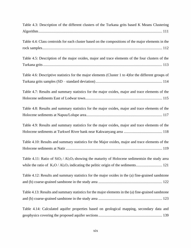
Table 4.3: Description of the different clusters of the Turkana grits based K Means Clustering

Algorithm .................................................................................................................................... 111

Table 4.4: Class centroids for each cluster based on the compositions of the major elements in the

rock samples................................................................................................................................ 112

Table 4.5: Description of the major oxides, major and trace elements of the four clusters of the

Turkana grits ............................................................................................................................... 113

Table 4.6: Descriptive statistics for the major elements (Cluster 1 to 4)for the different groups of

Turkana grits samples (SD – standard deviation) ....................................................................... 114

Table 4.7: Results and summary statistics for the major oxides, major and trace elements of the

Holocene sediments East of Lodwar town .................................................................................. 115

Table 4.8: Results and summary statistics for the major oxides, major and trace elements of the

Holocene sediments at Napuu/Lolupe area................................................................................. 117

Table 4.9: Results and summary statistics for the major oxides, major and trace elements of the

Holocene sediments at Turkwel River bank near Kakwanyang area ......................................... 118

Table 4.10: Results and summary statistics for the Major oxides, major and trace elements of the

Holocene sediments at Natir ....................................................................................................... 119

Table 4.11: Ratio of SiO2 / Al2O3 showing the maturity of Holocene sedimentsin the study area

while the ratio of K2O / Al2O3 indicating the pelitic origin of the sediments ............................ 121

Table 4.12: Results and summary statistics for the major oxides in the (a) fine-grained sandstone

and (b) coarse-grained sandstone in the study area .................................................................... 122

Table 4.13: Results and summary statistics for the major elements in the (a) fine-grained sandstone

and (b) coarse-grained sandstone in the study area .................................................................... 123

Table 4.14: Calculated aquifer properties based on geological mapping, secondary data and

geophysics covering the proposed aquifer sections .................................................................... 139

xx

Table 4.15: Minimum and maximum porosity values of various geological materials based on

Todd, 1980 .................................................................................................................................. 142

Table 4.16: Physico-chemical results for samples collected in the dry season of February 2018 for

the Turkwel River shaded fields are values that exceed guideline values for drinking water, and

'nd' refers to not detected. The samples were arranged (left to right) from upstream to downstream

..................................................................................................................................................... 146

Table 4.17: Physico-chemical parameters results during the February 2018 dry season for the SAA

and IA (2452 and 2460); (the shaded values exceed thedrinking water guidelines of KEBS (2014)

and WHO (2011)) ....................................................................................................................... 148

Table 4.18: Physicochemical parameters for the SAA in the wet season (shaded fields indicate

values that exceed the guidelines for drinking water) ................................................................ 149

Table 4.19: Physico-chemical parameters for the SAA in the dry season (February 2019 - shaded

values exceed the KEBS and WHO guidelines for drinking water) ........................................... 150

Table 4.20: Physico-chemical parameters for the TGSA during the wet and dry seasons (shaded

values exceed the KEBS (2014) and WHO (2011) guidelines for drinking water) .................... 152

Table 4.21: Results for the intermediate aquifer physico-chemical parameters in the wet season

(the shaded fields are values that exceed guideline values for drinking water of KEBS (2014) and

WHO (2011) ............................................................................................................................... 154

Table 4.22: Results for the intermediate aquifer measured water quality parameters of February

2019 (the shaded values exceed thedrinking water guidelines of KEBS (2014) and WHO (2011))

..................................................................................................................................................... 155

Table 4.23: Water quality parameters for the deep aquifer during the dry and wet seasons

(highlighted values exceed the KEBS (2014) and WHO (2011) guideline value for drinking water)

..................................................................................................................................................... 156

Table 4.24: Groundwater samples with variations in hydrochemical facies between the wet and the

dry season.................................................................................................................................... 163

xxi

Table 4.25: Water quality index (a) in the wet season and (b) in the dry season for the SAA, IA,

TGS and the DA, and for the boreholes and handpumps with an unknown depth ..................... 165

Table 4.26: Institutional groundwater supply sources with NO3 levels >5.0 mg/L in the wet and

dry seasons .................................................................................................................................. 178

Table 4.27: Descriptive statistics for δ18O and δ2H in rainfall and surface water in the Lodwar and

its environs (n/a for median and standard deviation values represent one sample available for

analysis) ...................................................................................................................................... 182

Table 4.28: Descriptive statistics Results for oxygen-18, 2H and 3H groundwater samples in the

SAA, TGSA, IA, DA, and for wells with unknown depth (DU) ................................................ 184

Table 4.29: Regression results from the shallow alluvial aquifer (SAA), Turkana grits shallow

aquifer (TGSA), intermediate aquifer and for the wells with unknown depth (DU) relative to the

GMWL and LWML .................................................................................................................... 192

xxii

LIST OF ABBREVIATIONS AND ACRONYMS

Abbreviation Meaning

AAS Atomic Absorption Spectroscopy

Al Aluminium

As Arsenic

ASAL Arid and semi-arid land

asl Above Sea Level

BCM Billion cubic meters

Bh Borehole

Ca Calcium

CF Continuous flow

CKR Central Kenyan Rift

Co Cobalt

Cr Cronium

Cu Copper

DA Deep aquifer

DEM Digital elevation model

EC Electrical Conductivity

EPA Environmental Protection Agency

FAO Food Agricultural Organization

GMWL Global meteoric water line

GNIP Global Network of Isotopes in Precipitation

GPS Geographic Positioning System

GSD Ground Sampling Distance

HCA Hierarchical Cluster Analysis

Hp Hand pump

IA Intermediate Aquifer

IAEA International Atomic Energy Agency

ICRAF International Centre of Agriculture and Forestry

IRMS isotope ratio mass spectrometer

JICA Japanese International Corporation Agency

K Potassium

KEBS Kenya Bureau of Standards

KISEDP Kalobeyei Integrated Socio and Economic Development Programme

Km2 Square kilometre

KNBS Kenya National Bureau of Statistics

KPHC Kenya Population and Housing Census

LAAS Lodwar Alluvial Aquifer System

LMWL Local meteoric Water Line

xxiii

LOWASCO Lodwar Water and Sewerage Company

LSC Liquid scintillation counter

m2 Square meter

MCM Million Cubic Meter

Mg Magnesium

mg/L Milligram per litre

Mn Manganese

Mo Molybdenum

MWI Ministry of water and Irrigation

MWL Meteoric Water Line

Na Sodium

NAS Nairobi Aquifer System

NDMA National Drought Management Authority

NE North East

NGO Non-Governmental Organization

Ni Nickel

NKR Northern Kenyan Rift

NW North West

P Phosphorous

Pb Lead

PCA Principal Component Analysis

PPL Plane polarised light

RTI Radar Technologies International

S Sulphur

SAA Shallow Alluvial Aquifer

SDD Silicon Drift Detector

SE South East

Se Selenium

SPA Service Provision Agreement

SPSS Statistical Package for Social Sciences

SSA Sub-Saharan African

SWC soil water content

TC/EA Temperature conversion elemental analyser

TCG Turkana County Government

TGSA Turkana Grit Shallow Aquifer

Ti Titanium

TU Tritium units

UAV Unmanned-aerial vehicles

UNESCO United Nations Educational, Scientific and Cultural Organization

UNHCR United Nations High Commission for Refugees

USA United States

xxiv

VES Vertical Electrical Sounding

WHO World Health Organization

WQI Water Quality Index

WRA Water Resources Authority

WTF Water table fluctuation

XPL Crossed polarised light

XRF X-ray fluorescence

Zn Zinc

xxv

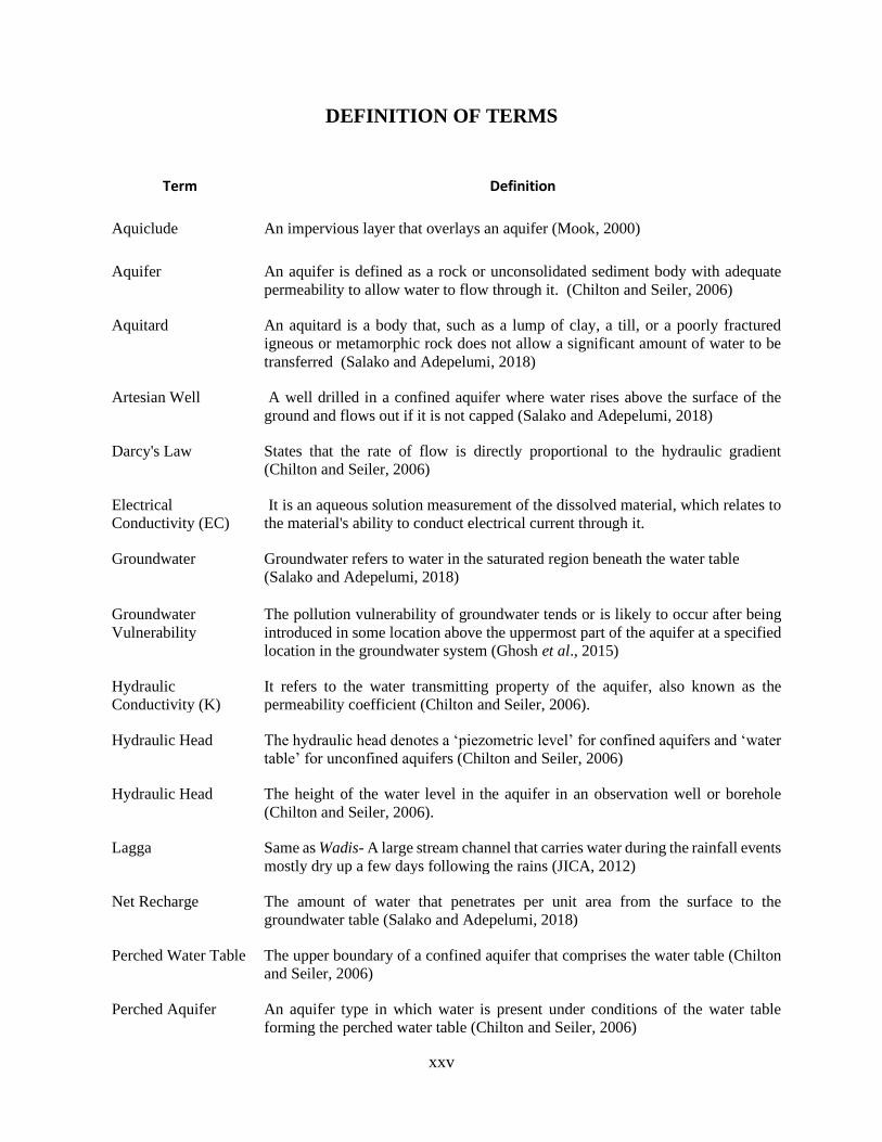
DEFINITION OF TERMS

Term Definition

Aquiclude An impervious layer that overlays an aquifer (Mook, 2000)

Aquifer An aquifer is defined as a rock or unconsolidated sediment body with adequate

permeability to allow water to flow through it. (Chilton and Seiler, 2006)

Aquitard An aquitard is a body that, such as a lump of clay, a till, or a poorly fractured

igneous or metamorphic rock does not allow a significant amount of water to be

transferred (Salako and Adepelumi, 2018)

Artesian Well A well drilled in a confined aquifer where water rises above the surface of the

ground and flows out if it is not capped (Salako and Adepelumi, 2018)

Darcy's Law States that the rate of flow is directly proportional to the hydraulic gradient

(Chilton and Seiler, 2006)

Electrical

Conductivity (EC)

It is an aqueous solution measurement of the dissolved material, which relates to

the material's ability to conduct electrical current through it.

Groundwater Groundwater refers to water in the saturated region beneath the water table

(Salako and Adepelumi, 2018)

Groundwater

Vulnerability

The pollution vulnerability of groundwater tends or is likely to occur after being

introduced in some location above the uppermost part of the aquifer at a specified

location in the groundwater system (Ghosh et al., 2015)

Hydraulic

Conductivity (K)

It refers to the water transmitting property of the aquifer, also known as the

permeability coefficient (Chilton and Seiler, 2006).

Hydraulic Head The hydraulic head denotes a ‘piezometric level’ for confined aquifers and ‘water

table’ for unconfined aquifers (Chilton and Seiler, 2006)

Hydraulic Head The height of the water level in the aquifer in an observation well or borehole

(Chilton and Seiler, 2006).

Lagga Same as Wadis- A large stream channel that carries water during the rainfall events

mostly dry up a few days following the rains (JICA, 2012)

Net Recharge The amount of water that penetrates per unit area from the surface to the

groundwater table (Salako and Adepelumi, 2018)

Perched Water Table The upper boundary of a confined aquifer that comprises the water table (Chilton

and Seiler, 2006)

Perched Aquifer An aquifer type in which water is present under conditions of the water table

forming the perched water table (Chilton and Seiler, 2006)

xxvi

Porosity Porosity within unconsolidated sediments or sedimentary rocks refers to the

percentage of open space. In sediments or sedimentary rocks, primary porosity

often refers to the spaces between grains, while secondary porosity refers to

porosity that developed after the rock was formed, i.e. fractures. The porosity of

volcanic rock is often associated with vesicles, whereas limestone may have

additional porosity associated with fossil cavities (Chilton and Seiler, 2006).

Recharge The entry of water into the saturated zone (Mook, 2000)

Recharge Recharge refers to as the entry of water into the saturated zone (Mook, 2000)

Specific Storage Specific storage refers to the amount of water released or taken into storage from

the aquifer per unit volume of the aquifer and per unit change in the hydraulic head

(Chilton and Seiler, 2006).

Specific Yield (Sy) Specific yield refers to the drainable porosity of an aquifer and is represents the

ratio of the volume of water drained by gravity after saturation (Salako and

Adepelumi, 2018)

Storage Coefficient Aquifer Storage Coefficient or Storativity (S) is the volume of water released from

storage per unit area of an aquifer per unit change in the hydraulic head (Mook,

2000).

Storativity The amount of water discharged from storage per unit of aquifer or aquitard

surface area per unit of hydraulic head decline (Salako and Adepelumi, 2018)

Transmissivity The aquifer's transmissivity (T) refers to the amount of water transmitted laterally

through the aquifer unit by full saturation of the aquifer under the hydraulic

gradient (Salako and Adepelumi, 2018).

Unsaturated Zone Refers to the part of the subsurface that is above the water table level and is

partially saturated, i.e. in the pore spaces between sediment grains, contains both

air and liquid water (Chilton and Seiler, 2006).

Wadis A channel of a watercourse that is dry except during periods of rainfall (Aboubaker

et al., 2013)

Point source

pollution

Point sources of pollution refer to the discharge of contaminants into the

groundwater through a pipe, ditch, discrete fissure, tunnels, concentrated animal

feed, and municipal wastewater (Garba Abdullahi et al., 2014; Islam et al., 2017)

Non-point source

pollution

Nonpoint sources may result from agricultural chemicals (fertilizers and

pesticides) through surface runoff, precipitation, atmospheric deposition, seepage,

drainage, or hydrological modification (Islam et al., 2017).

1

1 CHAPTER ONE: INTRODUCTION

1.1 Background

Groundwater resources have recently gained much attention globally as an important source of

water supply for domestic, industrial and agricultural water demands (Al-Ruwaih, 2017; Tlili-zrelli

et al., 2018; Wu et al., 2015). Groundwater supplies account for one-third of all freshwater

consumption worldwide, with an estimated consumption of 36%, 42% and 27% for domestic,

agricultural and industrial uses, respectively (Taylor et al., 2012). Today, about half of the

megacities in the world and hundreds of major cities on all continents rely on groundwater for the

above major uses (Jaroslav and Van der Gun, 2004), while rural communities and small towns rely

on it to supply domestic water, particularly in arid areas (UNESCO, 1998). The hydrogeological

setting of groundwater systems across the globe is unique to every region (Jaroslav and Van der

Gun, 2004; Liu et al., 2018; Shirazi et al., 2015).

Studies have revealed that the natural groundwater quality and geochemical characteristics of

aquifers are consistent with the geology of the area (Chae et al., 2004). Generally, shallow

groundwater systems are more vulnerable to natural and anthropocentric factors (Khatri and Tyagi,

2014) that affect both groundwater quality and quantity. Climate influences groundwater systems

directly through recharge from precipitation and indirectly by variations in groundwater use (i.e.

increased abstraction during droughts) (Andrés-Doménech et al., 2015; Taylor et al., 2012).

Increased human activities have led to land-use changes that have modified the climate, resulting

in increased variability in precipitation (Tague et al., 2008), soil moisture, surface and groundwater

(Taylor et al., 2012). In addition, sustainable groundwater development is continuously threatened

by a population increase, competing demands for water, and climate change (Dennehy et al.,

2015). Therefore, sustainable groundwater management strategies require interdisciplinary science

that provides accurate knowledge and tools for informed decision-making.

1.1.1 Global Perspectives

Globally, groundwater resources are still poorly assessed and, in many cases, are not managed in

a sustainable manner (Famiglietti, 2014). Four major hydrogeological settings define the

distribution of groundwater resources in the world; basement, sedimentary basins, high relief

folded mountain and volcanic regions (Jaroslav and Van der Gun, 2004). Unlike deep

2

groundwater, shallow groundwater systems are common in most places (Famiglietti, 2014;

Jaroslav and Van der Gun, 2004).

In arid areas worldwide, alluvial aquifers in wadis and river plains are important groundwater

resources (Van der Gun, 2010). Alluvial aquifers are often limited in width and thickness and are

the easiest to exploit of all the aquifer systems due to the shallow water table, good drinking water

quality and significantly high yields. Most alluvial aquifers comprise sand and gravel and mostly

unconfined. In ASAL regions, alluvial aquifers in the valleys of seasonal or ephemeral streams

often have permanent subsurface flows (Jaroslav and Van der Gun, 2004). These aquifers may

also receive additional recharge by infiltration of excess irrigation water, sometimes contributing

the most recharge (González-Trinidad et al., 2017). Thus, they are highly vulnerable to human-

induced pollution (Goni et al., 2019; D. Zhang et al., 2019). Furthermore, strong hydraulic links

with rivers and streams characterize alluvial aquifers, resulting in the exchange of water between

seasons; i.e. streams recharge the aquifers in the wet season and are drained in the dry season

(Jaroslav and Van der Gun, 2004). This process makes the alluvial aquifers vulnerable to rainfall

and streamflow variability (Van der Gun, 2010). Sustainable development of groundwater sources

in alluvial aquifers, therefore, requires a detailed understanding of their hydrogeological

characteristics (Liu et al., 2018; Shirazi et al., 2015), water quality and groundwater chemistry

(Abid et al., 2011; Aghazadeh et al., 2017), as well as their interactions with the river systems

(Atuahene, 2017; Hinzman et al., 2000; Teng et al., 2018).

1.1.2 Regional Perspectives

Groundwater is a vital source of water supply in Africa (MacDonald and Adelana, 2008),

especially in ASALs, where surface water resources are limited (Adelana et al., 2011). Indeed,

sub-Saharan Africa is a region that depends largely on groundwater (Lapworth et al., 2017; Xu et

al., 2019) and has extensive drought-prone areas (Foster et al., 2012) such as Somalia, Burundi,

Niger, Ethiopia, Mali and Chad (Shiferaw et al., 2014). Therefore, the successful development of

sustainable groundwater supplies is crucial for the continent's future supply of safe water,

economic growth, and food security (MacDonald and Adelana, 2008). The major setback,

however, to achieving sustainable groundwater development and management is the lack of

scientific understanding of the groundwater resources (MacDonald et al., 2012; Xu et al., 2019)

indicated that the groundwater resources in Africa are distributed unevenly with the largest

aquifers being the North Africa’s sedimentary aquifers, including Algeria, Libya, Egypt and what

3

was then Sudan (current Sudan and South Sudan). Alluvial aquifers hosted in unconsolidated

sediments form the vast majority of the sedimentary aquifers (MacDonald and Davies, 2000). They

occur in riparian zones of ephemeral and perennial rivers and comprise important groundwater

resources in sub-Saharan Africa (Lapworth et al., 2017).

In terms of water quality, urban groundwater is generally susceptible to human pollution. Due to

insufficient waste management, the shallow urban groundwater in Africa is often very poor

(Lapworth et al., 2017) and source protection (Ochungo et al., 2019), posing a significant health

risk to users (Varol and Şekerci, 2018). Although alluvial aquifers are essential resources in Africa

(MacDonald and Adelana, 2008), they are the least investigated (Lapworth et al., 2017). Few

studies of alluvial aquifers have been undertaken in the northern, western and southern African

regions and very few in the East African region (Xu et al., 2019).

1.1.3 National Perspectives

Groundwater resources in Kenya are becoming increasingly important due to the increasing

population (Falkenmark, 2019), infrastructural development, pollution of surface water (Bai et al.,

2016) and increased droughts caused by climate change (Taylor et al., 2012). About 80% of the

country is covered by arid and semi-arid lands faced with significant water scarcity (NDMA, 2016;

World Bank, 2018). The rainfall ranges from less than 200 mm in northern Kenya to more than

1800 mm in the region of Mt. Kenya, with an annual average of 630 mm (Koskei et al., 2018;

Opiyo et al., 2015). It is estimated that the 2016-2017 drought affected about 3.4 million people

living in arid and semi-arid areas across 23 of the 47 counties in the country (NDMA, 2016). The

recent drought events in the country (NDMA, 2016) have resulted in an increased focus on the

development of the country’s groundwater (REACH, 2015) to expand the existing water supplies.

Generally, the groundwater resources are unevenly distributed both in time and space, a situation

that has been exacerbated by climate variability (World Bank, 2018). Besides, very few studies

have been undertaken to understand groundwater resources (World Bank, 2018) accurately.

The occurrence and distribution of the groundwater resources in Kenya are controlled majorly by

geology (Kuria, 2011). Intrusive rocks and volcanic flows cover the Rift Valley and Central

Kenya; sedimentary rocks characterize coastal and northern Kenya, while metamorphic rocks are

localized in eastern Kenya (Kuria, 2011). Groundwater is confined within the Rift Valley by

lacustrine sediments, weathered and fractured zones in volcanic rocks, and sediments interbedded

4

between volcanic rocks (Kuria, 2013). According to Kuria (2013), the rift valley's aquifers include

the Turkana aquifer, the Baringo-Bogoria aquifer, the Nakuru aquifer, and the Magadi aquifer.

There is no single identified aquifer with significant groundwater in the areas covered by the

basement rocks. The piezometric map indicates that the aquifer within the basement rocks is

localized; examples of these aquifers can be found near Isiolo, Meru, Embu, Wote, and Kitui

(Kuria, 2013). Under the geological conditions of the basement terrains, groundwater occurs in

weathered zones above the crystalline basement rocks, fractured zones within the crystalline

bedrock, and alluvial deposits along the main drainage channels. (Kuria, 2011).

The major sedimentary aquifers in Kenya include; Lotikipi and Lodwar aquifers (Up to 80 deep),

Tiwi aquifer (<70 m deep), Gongoni-Msambweni aquifer (40-100 m deep), Baricho aquifer (25-

60 m deep), and the Merti aquifer 110-180 m deep) (Kuria, 2011). The renewable groundwater in

the country is estimated at 1.04 BCM per annum, and about 0.18 BCM (17%) is currently being

utilized (MWI, 2013; World Bank, 2018). Kuria (2011) plotted a transmissivity map using data

from the national groundwater database. This map shows that the transmissivities of groundwater

in drilled boreholes in Kenya range from <1.2 to 1598.7 m2/day, with the largest values observed

within the sedimentary aquifers. The Lotikipi, Lodwar and Tiwi aquifers are sedimentary

(consolidated/unconsolidated) aquifers with transmissivities ranging from 10 to 600 m2/d (Kuria,

2011).

Although the groundwater resources in Kenya have the potential to boost water supplies, its

exploitation is limited due to naturally poor water quality (Kuria, 2011; MWI, 2013; World Bank,

2018), pollution in urban centres (Ochungo et al., 2019; Olago, 2018), saline intrusion in coastal

areas (Ochungo et al., 2019), and limited knowledge of the occurrence of the groundwater in the

country (Olago, 2018; World Bank, 2018). Understanding the aquifer chemistry and identifying

the various sources of the chemical components in the groundwater is important for its

geochemical characterization (Chenini et al., 2010; Selvakumar et al., 2017). However, in Kenya,

very few studies investigating aquifer hydrogeochemistry have been undertaken in volcanic

(Kanda and Suwai, 2013; Karegi et al., 2018; Maina and Gaciri, 2010) and sedimentary areas

(Comte et al., 2017; Muthuka, 1994), and fewer in metamorphic areas. Hove and Ongweny (1974)

investigated Kenya's groundwater quality based on total dissolved solids. Olaka et al. (2016)

investigated the groundwater fluoride enrichment within the Central Kenya Rift - an active rift

5

setting. Groundwater quality studies have also been conducted in coastal regions of Kenya

(Makokha, 2019; Muthuka, 1994; Mzuga et al., 2001).

Rainfall-surface water interactions of alluvial aquifers have not been studied, yet such knowledge

is important in the understanding of aquifers recharge characteristics and for the determination of

impacts of rainfall and streamflow variability on groundwater. However, few studies have focused

on the investigation of groundwater isotopes in Kenya (Avery and Tebbs, 2018; Doust and

Sumner, 2007; Henkes et al., 2018; Nyende, 2013; Nyilitya et al., 2020; Ochungo et al., 2019;

Oiro et al., 2018; Sklash and Mwangi, 1991), and none has been carried out in Turkana county.

1.2 Statement of the Problem

Turkana County, situated in the north-western Kenya, is classified as an arid and semi-arid land

(ASAL) with very erratic, low (263 mm/yr.) and unreliable rainfall throughout the year (Opiyo,

2014). The County majorly depends on groundwater resources for water supply (JICA, 2012). The

steadily increasing demand for water from the rapid growth of urban populations, businesses and

emerging oil development operations has resulted in an unprecedented high demand for water in

an arid region (Olago, 2018). With this regard, the understanding of the groundwater resources

within Lodwar municipality and its environs is critical for the development of safe and reliable

groundwater supplies.

Groundwater sources (boreholes and handpumps) in Turkana County are developed mainly along

the major rivers (Turkwel and Kerio Rivers) and major laggas (JICA, 2012). Within Lodwar

Municipality, boreholes and handpumps have been developed on the riparian zones of the Turkwel

River (Hirpa et al., 2018; Olago, 2018) to abstract groundwater from the alluvial aquifer whose

hydrogeological characteristics are not fully understood (Olago, 2018). According to RTI (2013),

a shallow aquifer, within multi-layered fresh and weathered volcanic structures juxtaposed with

river sediments and Turkana grits close to the basement, underlies Napuu village east of Lodwar

town. The storage capacity of the Napuu shallow Lodwar aquifer was estimated to be 10 billion

cubic meters (BCM) per year, with an estimated recharge of 1.2 BCM/year (RTI, 2013). These

values are extremely high, necessitating a detailed study in the area to obtain accurate aquifer

storage and recharge estimates. UNESCO drilled three confirmatory boreholes (RTI 1, RTI 2 and

RTI) and conducted test pumping. Of these, RTI 1 is within the current study area and was drilled

to a depth of 47 m with an aquifer thickness of 20 m between 27- 47 m below ground level.

6

Although the findings of this study have been widely criticised owing to the methodology used

and unrealistic storage and recharge estimates (Avery, 2013), the drilling and test pumping results

provide important hydrogeological information of Lodwar and its environs that was initially

unknown. The analysis of the cross-sections revealed a possible replenishment correlation

dynamic between the Lodwar Aquifer and the Turkwel River (RTI, 2013). The surface water-

groundwater dynamics in Lodwar and its environs require further investigation to determine

specific correlations. A further study will unveil the aquifer’s structure and geometry,

hydrogeological characteristics, accurate storage estimates and delineation of aquifer boundaries.

The ten boreholes used for drinking water supplies in Lodwar are all located within a radius of 10

km from the town area (Olago, 2018), indicating that some parts of the municipality lie on top of

its groundwater resource. Currently, Lodwar municipality has no sewerage facility and a functional

waste disposal system (Hirpa et al., 2018), posing a risk of pollution of the shallow alluvial aquifer.

Lack of a proper sewage system contributes greatly to nitrate and faecal contamination of shallow

groundwater (Heiß et al., 2020). Further, no comprehensive water quality studies have been

undertaken to date for the shallow aquifer in Lodwar and its environs. Although Turkwel River

has been hypothesised to replenish the groundwater of the Lodwar alluvial aquifer, the

geochemical correlation and seasonal groundwater chemistry dynamics need to be established.

The hydrogeochemistry and vulnerability to pollution status of this aquifer is unknown, and thus

an urgent need for the determination of prevailing water quality, hydrochemical characterization,

and the determination of natural and human-induced pollution.

An aquifer system's rainfall-surface water-groundwater interaction provides data on the amount of

recharge attributed to rainfall and surface water (Atuahene, 2017; Meng et al., 2019; Teng et al.,

2018). It provides an opportunity to measure and quantify base flows and influxes between the

groundwater and surface water. Seasonal water table changes in the Lodwar aquifer is unknown,

and it is currently not possible to determine the extent to which climate variability influences the

system (Newman, 2019; Subramani et al., 2009; Xi et al., 2018). The quasi-perennial Turkwel

River that originates from Mt. Elgon region has been suspected to be the main source of recharge

to the shallow aquifer within Lodwar (Hirpa et al., 2018; JICA, 2012; Olago, 2018). However, the

specific recharge sites, and the effects of the ‘drying-up’ periods every year (Hirpa et al., 2018),

are unknown. Further, increasing populations, the planned expansion of irrigation activities (Ocra,

2015), warming temperatures and reduced precipitation linked to global warming may also

7

upsurge the risk of water scarcity in the Turkwel, resulting in reduced surface water and a

subsequent decrease in the groundwater recharge (Hirpa et al., 2018). The uncertainties

surrounding the systemic interaction between the Turkwel River and the underlying Lodwar

Alluvial Aquifer needs to be determined. Besides, no study has been undertaken in the study area

related to groundwater interaction regimes.

1.3 General and Specific Objectives

General Objective

The main objective of the study was to establish the hydrogeological characteristics of the Lodwar

Alluvial Aquifer System (LAAS) and its vulnerability to climate variability and anthropogenic

risks and uncertainties in the context of sustainable management.

Specific Objectives

The specific objectives for the research are to: -

1. Determine the hydrogeological characteristics of the Lodwar Alluvial Aquifer System;

2. Characterize the aquifer hydrogeochemistry, and to determine its susceptibility to

pollution;

3. Establish rainfall-surface water-groundwater interaction and recharge characteristics of the

aquifer; and

4. Develop a conceptual aquifer geometry model

Research Questions

The following research questions were formulated for this research:

1. What are the hydrogeological characteristics of the Lodwar Alluvial Aquifer System?

2. What are the hydrogeochemical characteristics of the LAAS and its susceptibility to

pollution?

3. What are the rainfall-surface water-groundwater interaction dynamics and recharge

characteristics in the LAAS?

4. Can we develop a conceptual aquifer geometry model using the derived datasets from this

research?

8

1.4 Justification and Significance

Justification

In the initial stages of the preparation of a sustainable groundwater development plan, scientific

understanding of the hydrogeological characteristics of an aquifer has an important role. These

include groundwater occurrence and distribution in its geological setting, and aquifer

characteristics such as extent, lithology, aquifer media, transmissivity, yields, depths, storage,

specific capacity, recharge, and discharge characteristics. These characteristics have not been

studied on a spatial scale in the Lodwar Alluvial Aquifer System (LAAS), although it is being

abstracted for water supplies; there are only point source data on aquifer characteristics from

drilled boreholes in the area which on their own cannot inform on aspects such as aquifer extent,

recharge and discharge characteristics. Furthermore, delineation of aquifer boundaries based on

the scientific understanding of the hydrogeological characteristics are critical tools for aquifer

protection, sustainable groundwater management, and land-use planning (Alam and Ahmad,

2014).

The geochemistry of groundwater is an essential factor in determining its geochemical evolution

(Hamlat and Guidoum, 2018) and use for several purposes, such as domestic, irrigation, and

industrial uses (Mostafa et al., 2017). Aquifer hydrogeochemistry contributes to the understanding

of the groundwater facies and aquifer processes in a region and reveals the sources of chemical

components in groundwater and its quality. The shallow nature and highly permeable geology

overlying this aquifer make it extremely important to both understand its vulnerability to pollution

and to delineate potential pollution sources. Thus, the spatial and temporal characterization of the

hydrogeochemistry of the Lodwar Alluvial Aquifer System will not only make it possible to assess

its suitability for domestic, drinking, industrial and irrigation purposes but also to determine the

geochemical processes underpinning its characteristics, thus providing the much-needed evidence

necessary for successful development and management of safe water supplies.

Rainfall - surface water - groundwater interactions are crucial components of alluvial aquifer

systems. The estimation of modern-day aquifer recharge rates for shallow aquifers is critical when

evaluating the sustainability of groundwater resource development (Chilton and Seiler, 2006;

Jaroslav and Van der Gun, 2004), the recharge and discharge characteristics of the LAAS are

currently unknown. Several studies have proposed potential linkages between the Turkwel River

9

and the LAAS (Hirpa et al., 2018; JICA, 2012; Olago, 2018; RTI, 2013), but the current evidence

is insufficient for informed decision-making for the development and protection of the aquifer. In

addition, an understanding of aquifer recharge mechanisms and associated land-use linkages is

required for resource catchment-scale assessments, which form essential components for

integrated water resource management (Foster and Chilton, 2003). Isotopic analyses of oxygen-

18, deuterium and tritium in rainfall, surface water and groundwater samples are useful tools for

confirming the existing linkages among these systems, and to quantify the recharge from rainfall

and surface water. This kind of study has not done in the area; further, the impacts of current and

future climate variability and risks remain uncertain for the Lodwar Alluvial Aquifer System.

Currently, no aquifer conceptual model is available for the area of study. The aquifer conceptual

model for the LAAS will help to illustrate the hydrogeological and geochemical conditions

controlling the quantity and quality of its groundwater. The aquifer conceptual model derived from

the understanding of the hydrogeology, hydrogeochemistry, and the evaluation of the rainfall-

surface water-groundwater interaction is a tool that can be utilized by decision-makers in both

county and national levels for sustainable use and management of groundwater resources.

Significance

The elucidation of the hydrogeological characteristics of the Lodwar Alluvial Aquifer System will

provide the evidence-base for sustainable management of the system. Accurate information on the

aquifer storativity, recharge, and discharge mechanisms are crucial in planning current abstraction

to minimize future risks of water supply in Lodwar and its environs. Aquifer identification,

delineation, and protection of recharge zones is part of Vision 2030 environmental protection

goals, especially in arid and semi-arid regions of Kenya. This study will also contribute to the

ongoing groundwater studies in arid environments, especially in the sub-Saharan Africa region,

where knowledge of groundwater resources is much needed to ensure access to safe drinking water

supplies and achieve sustainable management.

Characterization of the hydrogeochemistry of the LAAS will help to discriminate natural and

anthropogenic influences on groundwater quality in the aquifer system. It will, therefore, facilitate

early detection, mitigation and elimination of contamination sources by the Turkana county

government to ensure that its people get sustainable access to safe water. The provision of clean

and safe drinking water to its citizens is a constitutional directive of the Government of Kenya.

10

Therefore, the findings of this study will contribute to its full realization in Lodwar and its

environs. The seasonal water quality monitoring conducted by this study and the accompanying

water quality index maps would form the basis for long-term groundwater monitoring and

development by the Water Resources Authority (WRA) and other agencies in the area. Developed

countries such as the United States, United Kingdom, Denmark, amongst others, have developed

the groundwater vulnerability maps for their entire countries. This study is a step for Kenya to

develop such maps for its groundwater resources. Identifying areas of good groundwater quality

contributes to SDG 6 of clean water and sanitation in the contexts of communities in Lodwar and

its environs. Furthermore, the key features of groundwater relevant to the SDGs that this study

aims to elucidate are its use, management, and sustainability.

Knowledge of the extent, recharge and discharge characteristics of the aquifer will help the

Turkana County Government to not only know the sustainable supply limits of the aquifer but also

to protect it and to plan the urban expansion into non-recharge and abstraction zones. This

information would enable the Turkana county government to plan for sustainable supply and to

adopt management options that consider the impacts of climate variability in the region. Very few

studies involving rainfall-surface water-groundwater interaction have been carried out globally,

especially in Sub-Saharan Africa, and this study will provide additional knowledge in future

studies. Lastly, the conceptual aquifer geometry model for the LAAS will be an excellent tool for

decision making in terms of monitoring, development, management, and protection of the aquifer

system.

1.5 Scope and Limitation of the Study

The study area covered the mid-section of the Turkwel watershed, centred on Lodwar municipality

and extending to its environs. Secondary data on groundwater quality, geological logs of drilled

wells, and test pumping data were obtained from the regional and sub-regional offices of the Water

Resources Authority (WRA) and from the water practitioners in the Turkana region, such as

Oxfam and the Catholic Diocese of Lodwar. Field geological and geophysical studies were

undertaken, and rock and water samples (groundwater, river and rainfall) were collected within

the 1040 km2 study area. Recharge characteristics and groundwater interaction processes were

determined using isotopic compositions of deuterium, oxygen-18 and tritium in water.

11

The major limitations of this study were data scarcity and inaccessibility. The hydrogeological

data of the area are generally limited, while that available contained numerous gaps. Missing

information for most borehole records included; geographic coordinates, drilled depth, borehole

logs, tested yields, water rest levels, and water quality information. Water table monitoring data

was available only for two boreholes (LOWASCO Bh 9 and Napuu Bh) for nine and six months,

respectively, limiting the application of the water table fluctuation method in this study.

Inaccessibility of boreholes and handpumps in some parts of the study area for water sampling was

also a challenge – the ongoing land tenure system has led to fencing off land areas and privatization

of water points.

1.6 The Layout of the Thesis

This study is presented in five chapters, as illustrated in the thesis layout (Figure 1.1). Chapter 1

provides the background of the study, including the global, regional and global perspectives of

groundwater, statement of the problem, study objectives, as well as justification and significance.

Chapter two describes the study areas in terms of location, geology and structures, climate,

groundwater and surface water resources, and land use activities, as well as a detailed literature

review of the thematic areas covered by the study. Chapter 3 presents the various methodologies

used for each specific objective, while Chapter 4 summarizes the research findings. Chapter 5

provides the main conclusions from all the chapters, implications for practice, and potential areas for

future research based on the critical findings of this study.

12

Figure 1.1: Layout of the thesis

13

2 CHAPTER TWO: LITERATURE REVIEW

2.1 Introduction

This chapter presents a detailed literature review of groundwater systems, with a particular focus

on volcano-sedimentary and alluvial aquifers. These aquifers comprise the hydrogeological

contexts of the research study area as specified in Chapter 1, section 1.2, and relate to the research

objectives of the thesis. The first part covers a global review of aquifer settings, types,

characteristics and geometries in volcano-sedimentary and alluvial terrains. The second part covers

the hydrogeochemistry and hydrochemical facies, aquifer processes, and vulnerability to pollution

within volcano-sedimentary aquifers and alluvial systems. Part three includes rainfall-surface

water-groundwater interactions, recharge estimation and age of groundwater, while part four

provides details of aquifer geometry modelling. An additional section of current approaches to

sustainable groundwater management comprises part five. Lastly, a summary of this chapter with

key highlights and gaps is presented.

2.2 Hydrogeological Characteristics of Aquifers

The lithological characteristics and hydraulic properties of an area control the groundwater

development within that area (Ahmed et al., 1998); therefore, hydrogeological conditions are

unique to every region around the world (Jaroslav and Van der Gun, 2004). The successful

development of groundwater and its optimum utilization requires an accurate understanding of

prevailing aquifer characteristics and properties (Ahmed et al., 1998; Chilton and Seiler, 2006).

An aquifer is a reservoir of groundwater composed of permeable geological units saturated with

water to provide usable quantities of water. Aquifers transport groundwater from recharge to

discharge zones and serve as a storage medium for current and future use. Globally, two major

types of aquifers exist; confined and unconfined. A confined aquifer is underlain by an aquiclude

and is mostly unconfined at its outcropping edges that contribute a significant amount of recharge

during rainfall events (Chilton and Seiler, 2006). Confined aquifers may also receive recharge

through upper and lower leaky confining layers. The groundwater in a confined aquifer is subjected

to hydrostatic pressure that induces increased pore pressure that is higher than atmospheric

pressure (Ahmed et al., 1998), causing the water in a well to rise beyond the upper level of the

14

aquifer. In instances where there is enough pressure to force the water to flow at the land surface,

these are referred to as artesian wells. As a result, the well's or aquifer's response to changes in

atmospheric pressure is variable and directly proportional to the degree of aquifer confinement

(pore pressure) containment, as well as hydraulic and storage characteristics. Confined aquifers

often have low storativity values ranging from 0.01 to 0.0001 (Salako and Adepelumi, 2018).

Unconfined aquifers, also known as phreatic aquifers, do not have upper impermeable layers but

are underlain by an aquiclude (Chilton and Seiler, 2006; Salako and Adepelumi, 2018). Thus, they

can be recharged locally from rainfall by infiltration and percolation of the rainwater through

interconnected pores. In comparison with confined aquifers, groundwater in an unconfined aquifer

is more susceptible to anthropogenic pollution, linked to the possibility of direct migration of

dissolved pollutants to recharge water. Unconfined aquifers have storativity values > 0.01 (Salako

and Adepelumi, 2018). Schematic illustration of confined and confined aquifers is given in Figure

2-1. Perched aquifers are distinct types of unconfined aquifers occurring above the regional water

table (Salako and Adepelumi, 2018). Thus, when a low-permeability layer prevents the downward

water movement above it, they always exist above an unconfined aquifer or a confined aquifer in

the vadose zone. Perched aquifers are generally small and may not have sufficient storage to

support substantially good production.

15

Figure 2.1: Schematic illustration of the confined and unconfined aquifers (source: Salako and

Adepelumi, 2018)

A global review of aquifer types

Groundwater occurrence primarily depends on geology, geomorphology, weathering, and

adequate rainfall (both current and historical) (MacDonald et al., 2012). There are four geological

provinces for groundwater occurrence around the world: Precambrian “basement” rocks, volcanic

rocks, consolidated sedimentary rocks, and unconsolidated sediments (alluvial aquifers) (Chilton

and Seiler, 2006; Macdonald et al., 2016; Mook, 2000).

2.2.1.1 Precambrian “basement” aquifers

Precambrian basement aquifers develop within overlying weathered materials and fractured

bedrock of metamorphic and or intrusive origin (Wright, 1992). In tropical and sub-tropical

regions (Wright, 1992), deeply weathered crystalline bedrock aquifer systems occur within low-

latitude regions of Africa, South America and Asia (Taylor and Howard, 2000). About 40 % of

sub-Saharan Africa is underlying these aquifers (MacDonald et al., 2012) and are a significant

source of water for a quarter of a billion people in the region (MacDonald and Adelana, 2008;

Taylor et al., 2009). Across the tropics, including East Africa, weathered crystalline basement

16

aquifers maintain water supplies (Maurice et al., 2018). Transmissivities of crystalline basement

aquifers investigated by Maurice et al. (2018) in Tanzania and Uganda ranged from 10–1,000

m2/day, which were higher than observed in the majority of deeply weathered crystalline bedrock

aquifers (<10 m2/day). Generally, the basement aquifer systems are highly heterogeneous (Taylor

and Howard, 2000) and are characterized by considerably low yields (Wright, 1992).

2.2.1.2 Volcanic rock aquifers

In North America, especially Columbia Basin in the NW of the USA and parts of the Deccan

Plateau in India, volcanic aquifers are widespread around the world and are important groundwater

resources. These aquifers form in basin-like structures formed in volcanic regions with extensive

basalt-lava flows (Mook, 2000). Limited groundwater resources are often provided by volcanic

aquifers (Jaroslav and Van der Gun, 2004; Kebede et al., 2008). Increased groundwater abstraction

from deep artesian aquifers may reduce piezometric levels, resulting in mixing with shallow

groundwater overlying the aquifer (Mook, 2000). Volcanic rocks cover only 6% of the land area

in SSA and are mostly confined to eastern Africa (MacDonald et al., 2012) and were formed during

the Cainozoic period, associated with the opening of the rift valley in East Africa. The region's

volcanic aquifers include thick, complicated sequences of lava flows, sheet basalts, and pyroclastic

rock such as agglomerate and ash (MacDonald et al., 2012).

2.2.1.3 Sedimentary rock aquifers

Consolidated sediments make up some of the major aquifers in the world, consisting primarily of

younger Paleogene and Neogene and older Mesozoic or Palaeozoic formations of sandstone and

limestone (Chilton and Seiler, 2006; Mook, 2000). Aquifers are found in consolidated sediments

all over the world, including mountain belts such as the Andean, Alpine-Himalayan, and North

American cordilleras, as well as lowlands and plateau areas in northern Europe and Central China

(Chilton and Seiler, 2006; Foster and Chilton, 2003). Massive sedimentary aquifers in North Africa

contain a significant portion of Africa's groundwater (MacDonald et al., 2012), with the largest

groundwater reserves in Libya, Algeria, Sudan, Egypt, and Chad (MacDonald et al., 2012; Mook,

2000).

Depending on the degree of cementation, Paleogene and Neogene sandstones can range from loose

to highly consolidated rock (Chilton and Seiler, 2006). In such cases, secondary porosity caused

by fracture development can provide adequate permeability and storage to form productive aquifer

17

(Mook, 2000). On the other hand, limestones show solution enhancement of such fractures (karst)

in arid and semi-arid areas and coastal regions that make them prolific aquifers (Chilton and Seiler,

2006; Foster and Chilton, 2003). Due to both the main porosities and fractures enhanced by

weathering and dissolution, sandstone and limestone have high to very high permeability,

respectively (Chilton and Seiler, 2006). In sandstone and calcareous aquifers, the combination of

primary and secondary porosities results in rapid groundwater movement with velocities often

above 100 m / day (Chilton and Seiler, 2006; Mook, 2000).

2.2.1.4 Alluvial aquifers

Quaternary deposits occurring in alluvial plains and fans, river deltas, and glacio-fluvial deposits

usually consist of unconsolidated sediments that host numerous aquifers (Mook, 2000). Gravel

and sand dominate the formations with intercalations of silt, mud, and clay. The unconsolidated

sediments form some of the most important aquifers globally, hosting enormous volumes of

groundwater (Chilton and Seiler, 2006). The great examples of unconsolidated sedimentary

aquifers include, the Mekong, the Lower Indus and Ganges Brahmaputra valleys, the north

European plain, the Tigris-Euphrates, and the Nile valley (Chilton and Seiler, 2006; Macdonald et

al., 2016). In east Africa, the South Coast aquifer system (SC) is an excellent example comprising

unconsolidated coastal sediments (Oiro et al., 2018). These deposits are located in the world's

largest cities, such as Bangkok, Beijing, Cairo, Calcutta, Dhaka, Hanoi, Lima, Madras, and

Shanghai, and are supplied by groundwater from unconsolidated strata (Chilton and Seiler, 2006).

Aquifers are seldom simple homogeneous systems in unconsolidated strata but mainly composed

of discontinuous permeable layers of productive gravels and sands separated by less permeable

aquitard layers of clay and silt, reflecting the complex deposition history (Chilton and Seiler, 2006;

Hinkle and Survey, 1997). In such sequences, the shallowest aquifer may be the easiest and

cheapest to exploit, but it is also the most vulnerable to contamination (Chilton and Seiler, 2006).

Intricate groundwater flow patterns may be created by the presence of aquitards (Mook, 2000), but

the permeable layers may still have a degree of hydraulic continuity (Egan and Price, 2014), such

that pumping from one layer will affect the others, generating significant vertical head gradients

and leakage (Chilton and Seiler, 2006).

18

2.2.1.5 Heterogeneous composite “volcano-sedimentary” aquifers

Volcanic and sedimentary aquifers (volcano-sedimentary) comprise 55% (Jaroslav and Gun, 2004)

of the Worlds’ groundwater resources and are mainly distributed in ASALs. Aquifers of these

types include lavas and pyroclastic rocks coupled with alluvial-volcanic and alluvial fan deposits

(Chilton and Seiler, 2006). In the Horn of Africa (Djibouti), alluvial aquifers exist in the valleys

of wadis (intermittent streams), and they form complex volcano-sedimentary aquifers when they

approach volcanic aquifers (Aboubaker et al., 2013). In the Kenyan rift system, volcano-

sedimentary aquifers exist in the Turkana basin and within the Mesozoic sediments in the Dawa

basin at the Kenya-Ethiopia border (Kebede, 2005) located in the northern part of the country.

Sedimentary aquifers in the country are in northern Kenya and the coastal region (Kuria, 2011).

Turkana aquifer, Nakuru aquifer, Baringo-Bogoria aquifer, and Magadi aquifer are the aquifers in

the country's rift system (Kuria, 2011), where the Turkana aquifer includes a volcano-sedimentary

system. Within the Paleogene and Neogene volcanics, the volcano-sedimentary aquifers in the

northern parts of Kenya, and thick Miocene to Quaternary sediments are (Kebede et al., 2010a).

Aquifer characteristics and groundwater flow

Groundwater is rarely static, but rather moves slowly through aquifers (Chilton and Seiler, 2006)

due to changes in hydraulic head and differences in groundwater levels or pressure and is primarily

controlled by the permeability of the aquifer material (Shekhar, 2017). Darcy’s Law governs the

flow of groundwater through an aquifer. Darcy’s Law gives an accurate description of the flow of

groundwater in most naturally occurring hydrogeological conditions. Its relationship with

hydraulic gradient can be expressed as;

Q

A= 𝑞 =

−𝐾(ℎ1−ℎ2)

𝑙= −𝐾(∆ℎ/∆𝑙) Equation 2.1

Where, Q is the rate of flow through area A, K is the hydraulic

conductivity, h1 – h2 is the hydraulic head difference between two

measuring points, ∆h/∆l is the hydraulic gradient, and q is the

volumetric flow per unit surface area.

The direction of groundwater flow in an aquifer is perpendicular to equal-head lines (Chilton and

Seiler, 2006). Groundwater flow may occur in, for instance, a jointed sandstone or limestone

through fractures or spaces between the grains or a combination of the two (Egan and Price, 2014).

19

Borehole test pumping data is used to accurately determine aquifer parameters and lithological

characteristics (Shirazi et al., 2015) as well as to evaluate its potential (Jimenez and Chávez, 2004).

Specific characteristics of each aquifer in time and space can be defined based on aquifer properties

such as porosity, specific yield, aquifer storage, transmissivity, and hydraulic conductivity. The

hydraulic conductivity, flow path and gradient are significantly controlled by aquifer media,

according to Shirazi et al. (2015). Groundwater movement is usually due to variations in the

hydraulic head of an aquifer. Hydraulic heads are commonly measured in relation to an arbitrary

datum, which is frequently sea level (Chilton and Seiler, 2006).

Alluvial aquifers occur within the depositional basins of perennial and ephemeral streams in arid

and semi-arid areas, and the aquifer materials usually comprise sand, silts and gravel (Foster and

Chilton, 2003). Because of the high porosity of unconsolidated sediments in the range of 0.25 to

0.35 and the generally low horizontal hydraulic gradients of the alluvial plains, groundwater

velocities in the range of 0.003-0.1 m/day are common (Chilton et al., 2006). These low velocities,

combined with the significant distances travelled (tens to hundreds of kilometers), suggest that

much of the deeper groundwater in thick alluvial sequences was recharged several hundred to

several thousand years ago, resulting in old groundwater in such systems (Chilton and Seiler,

2006).

Natural groundwater discharge occurs in springs, in arid and semi-arid areas, and in some basins,

sub-surface flow into another basin can discharge significant amounts of groundwater into stream

channels, wetlands, and seasonal lakes. Abstracting groundwater can also contribute significantly

to groundwater discharge from water wells (Calvache et al., 2011; Yang et al., 2018). The

groundwater potential in an aquifer is a function of rock types constituting them (Ashraf et al.,

2018). In basement systems, groundwater potential is due to a combination of fractures and

weathered rock systems (Ashraf et al., 2018; MacDonald et al., 2012). In volcanic systems, the

groundwater potential depends mainly on the presence of fractures (Macdonald et al., 2016; Oiro

et al., 2018). In sedimentary systems, the main types of water-bearing rocks are usually sand,

sandstone, fractured or karstic limestone and dolomite (Ashraf et al., 2018). Generally, in most

arid and semi-arid terrains, limited groundwater recharge contrasts with vast groundwater reserves

created during the Pluvial periods of the Pleistocene (Jaroslav and Gun, 2004).

20

2.3 Hydrogeochemical Characteristics of Volcano-Sedimentary and Alluvial Aquifers

Groundwater chemistry is governed by factors such as rock water interaction – the formation

through which water flows, evaporation and concentration, dilution due to precipitation that may

result in changes in chemical compositions of groundwater (Ansari and Umar, 2019; Ashraf et al.,

2018; Maurice et al., 2018). The hydrogeochemistry of shallow alluvial aquifers in arid and semi-

arid areas is linked to the cumulative consequence of the rock-water interaction, dissolution of

soluble minerals, and nature and intensity of anthropogenic activities (Ansari and Umar, 2019;

Elango and Kannan, 2007; Vasu et al., 2017).

Determinants of natural groundwater quality and vulnerability of alluvial aquifers to

pollution

Groundwater quantity and quality, coupled with the climate change effects, are of major concern

for meeting the increasing demand for freshwater (Shirazi et al., 2015). Natural groundwater

quality varies significantly through periodic aquifer profile as a result of geology and the physical

and chemical processes that can affect salinity, temperature, pH levels, heavy metals, and organic

substances in the aquifer (Afzali et al., 2015; Aghazadeh et al., 2017; Ansari and Umar, 2019).

Physical and chemical processes that can have an impact on water quality include;

• During groundwater movement along the flow path, dissolved rocks and minerals are

transported and redeposited;

• Evaporation may cause an increased concentration of minerals and salts in the

groundwater;

• Chemical reactions in the aquifer leading to altered groundwater chemistry

Knowledge of prevailing groundwater quality plays a significant role in the early stages of a

groundwater sustainable development plan (Shirazi et al., 2015). Groundwater quality in volcanic

environments is a problem in most cases due to high fluoride concentrations above 1.5 mg/L

(Macdonald et al., 2016). Fluoride concentrations are high in volcanic rocks in Ethiopia's Rift

Valley. More generally, high fluoride groundwaters in the rift valley regions of Kenya and

Tanzania have led to health associated problems (Ashley et al., 2004; Coetsiers et al., 2009; Mbithi

et al., 2017; Olaka et al., 2016). Because of the rapid burial of alluvial sediments, groundwater

with high arsenic (As) levels has been associated with sedimentary rocks in reducing conditions

typical of alluvial and deltaic environments (Vivona et al., 2007). The most likely mechanism for

21

As release into groundwater in this environment is reductive dissolution of As-rich Fe oxy-

hydroxide (Vivona et al., 2007).

Groundwater pollution is a constant concern globally because aquifers, especially shallow alluvial

aquifers, are vulnerable (Kumar et al., 2014), especially those in the vicinity of urban areas (Al-

Shaibani, 2008). Nitrate is the most prevalent groundwater contaminant in shallow urban

groundwater (Kuroda and Fukushi, 2008). Nitrate in groundwater originates from agricultural

runoff from the use of fertilizers upstream of the aquifers. However, in urban areas where

agricultural fertilizers are absent, the common sources of nitrates are leaky sewage, septic tanks,

landfills and industrial spillage (Goudarzi et al., 2017; Kuroda and Fukushi, 2008). Contaminants

other than nitrogen in urban groundwater include fluoride (Ayenew, 2008; Brindha et al., 2011),

arsenic (Acharyya, 2002), heavy metals (Twarakavi and Kaluarachchi, 2005) and volatile organic

carbons (Kuroda and Fukushi, 2008).

The term “aquifer pollution vulnerability” was used by (Foster et al., 2012) to characterise the

intrinsic characteristics that determine the sensitivity of the groundwater system to being adversely

affected by an imposed pollutant load. However, the approach of Foster et al. (2012) also

distinguishes pollution vulnerability from pollution risk because pollution risk can stem from both

the aquifer's natural vulnerability and the pollution load that is or will be applied to the earth's

subsurface by human activities. As a result, an aquifer may be highly vulnerable while posing no

risk due to the absence of significant pollution loading, and vice versa (Jang et al., 2017).

Hydrochemical facies and rock water interactions

Complex water types have been observed in volcano-sedimentary aquifers (Aboubaker et al.,

2013). Evaluation of Na/Cl ratios reveal that halite dissolution is not the only source of Na+ and

Cl- ions in volcano-sedimentary aquifers in arid areas (Aboubaker et al., 2013). Other sources of

Na and Cl in alluvial aquifers are weathering of silicate minerals (Ashraf et al., 2018; Ramesh and

Gowri, 2012) and ion-exchange processes in the soil and aquifer matrix (Martínez and Bocanegra,

2002; Ramesh and Gowri, 2012). The dominant water types in volcanic aquifers are Na-HCO3,

Na-Mg-Ca-HCO3, and Na-Ca-HCO3 water types due to rock-water interactions (Morán-Ramírez

et al., 2016). In alluvial aquifers, Ca-HCO3 is a common water type (Al-Shaibani, 2008; González-

Trinidad et al., 2017; Hinkle and Survey, 1997; B. D. Li et al., 2015). Other dominant water types

in arid alluvial aquifers are Ca + Mg-HCO3 and Na + K-HCO3 (Ansari and Umar, 2019).

22

Groundwater from sedimentary aquifers has a good correlation between Ca and HCO3 (R2 = >0.7)

due to their high concentrations in the rocks, while volcanic aquifers often show weak correlations

between Ca and HCO3 (R2 = <0.1) (Vivona et al., 2007).

Fluoride concentrations in groundwater are higher, particularly in arid and semi-arid regions

(Adimalla et al., 2020). In volcano-sedimentary aquifers, F- concentrations exceeding the guideline

value for drinking water (1.5 mg/L) is a common challenge in groundwater (Adimalla et al., 2020;

Brindha et al., 2011; B. D. Li et al., 2015). Various variables, including rock chemistry, residence

time, well depth, preferential pathways to control the occurrence of high fluoride in groundwater

for the upward movement of deep groundwater. Flouride-rich minerals (fluorite or fluorspar

(CaF2), fluorapatite [Ca5 (OH, F) (PO4)3] and cryolite (Na3AlF6)) can release F- into groundwater

through weathering and rock-water interaction processes (Adimalla et al., 2020). Other fluoride-

bearing minerals include glaucophane, riebeckite and asbestos (chrysotile, actinolite,

anthophyllite) minerals from the biotite, muscovite, tourmaline, lepidolite, hornblende series

(Edmunds and Smedley, 2013). The processes of retention and leaching directly affect the

migration and exchange of fluoride from the soil to the water (Ansari and Umar, 2019). Apart from

high fluoride in groundwater, volcano-sedimentary aquifers exhibit very high iron exceeding 0.3

mg/L and manganese (> 0.1 mg/L) concentrations related to a strong anoxic condition caused by

the thick silt bed (Chae et al., 2004). Rock-water interaction is a process that strongly affects

hydrochemical facilities; solid phases (organic and inorganic) are the main sources of dissolved

constituents in groundwater in this process (Elango and Kannan, 2007) and, as groundwater moves

from recharge to discharge areas, a variety of chemical reactions with the solid phases occur.

Expected chemical reactions depend on the original chemical nature of the water, geological

formations, and residence time (Elango and Kannan, 2007). The chemical processes involved

during rock-water interactions are precipitation and dissolution, ion exchange processes,

oxidation, and reduction. Investigation of hydrogeochemistry of an aquifer helps to determine the

factors controlling the groundwater quality and the geochemical processes in an aquifer system

(Chae et al., 2004; B. D. Li et al., 2015; Subramani et al., 2009). Studies have revealed that the

groundwater quality and the geochemical characteristics of volcano-sedimentary and alluvial

aquifers are consistent with the geology of the area (Chae et al., 2004).

23

2.4 Rainfall-Surface Water-Groundwater Linkages and Recharge Estimation

The fresh groundwater resources of the world are hosted in shallow aquifers (Jaroslav and Van der

Gun, 2004) recharged by modern rainfall (Green, 2016). In addition to the associated impacts of

the natural environment and human activities (Green, 2016), changes in the global climate are

expected to affect the hydrological cycle, alter surface water levels, and replenish groundwater

systems (Taylor, 2013). The challenges of understanding the impacts of climate change on

groundwater systems are unique because these changes can, directly and indirectly, affect

groundwater resources and hydrogeological processes (Green, 2016; Taylor, 2013). Limited

observation data in many areas has made it difficult to accurately determine the extent and

direction of groundwater change due to climate impacts (Taylor 2013). Still, where they do exist,

they show that groundwater, along with surface water, is vulnerable to climate variability (Z. Chen

et al., 2004). Further research is required to support integrated groundwater management and

improve the understanding of climate and groundwater interactions.

Rainfall - surface water – groundwater interactions

The groundwater-surface water interaction in a basin plays a crucial role in understanding and

managing an aquifer system. Surface water and groundwater interact in two ways: rivers gaining

water from the groundwater flowing through the riverbed (base flows) and rivers losing water as

it flows out of the riverbed into a groundwater system (Taylor and Howard, 1996). Atmospheric

water vapour, rainfall and evapotranspiration patterns, soil water content (SWC) and temperature,

and surface runoff and river discharge (Bates et al., 2008) are the elements of the surface

hydrologic cycle (Figure. 2.1) that are impacted by climate change. Such changes in the

components of the global hydrological cycle's atmospheric and surface components are likely to

result in changes in the hydrological cycle of the subsurface within the world's soil, vadose zone,

and aquifers (van Dijk et al., 2017). The potential climate change effects on groundwater and its

sustainability are, however, poorly understood (Gleeson et al., 2012; Kotchoni et al., 2018).

Evapotranspiration and precipitation are particularly important because they directly affect

groundwater recharge and eventually affect human groundwater abstractions (Green, 2016). In

arid and semi-arid regions, minor changes in rainfall may lead to great recharge changes (Green,

2016). High temperatures, on the other hand, are likely to increase evapotranspiration, which may,

in turn, reduce the moisture content of the soil.

24

Current vulnerabilities in shallow groundwater resources in ASALs are strongly correlated with

precipitation variability (Green, 2016; Kundzewicz et al., 2008). The overall impacts of climate

variability on groundwater resources can be determined through an investigation of rainfall-surface

water-groundwater interactions. The interaction of these systems is gaining attention globally,

especially in the SSA region, due to increasing rainfall variability (Kebede et al., 2008).

Piezometric observations and stable-isotope ratios are useful approaches for investigating

groundwater interactions with rainfall and surface water (Taylor, 2013; Taylor and Howard, 1996).

Figure 2.2: Diagrammatic representation of the hydrological cycle, including rain-fed and

irrigated farming with potential abstraction of groundwater (Source: Green 2016)

25

Figure 2.3: Summary of hydrologic processes in rainfall - surface water - groundwater systemic

interactions

The analysis of stable isotope ratios of water (δ18O and δ2H) is useful for investigating rainfall -

surface water - groundwater interaction (Kebede, 2005). The distinction between the isotopic

content of evaporated and unevaporated waters allows for the detection of flow paths between

water bodies. When water evaporates from water bodies, isotope fractionation of the oxygen and

hydrogen that make up the water occurs, resulting in the enrichment of the water body by heavy

water isotopes of oxygen and hydrogen (Kebede et al., 2008). Unevaporated water bodies will

have lighter isotopic compositions than evaporated water bodies. In their study (Kebede, 2005)

noted progressive northward enrichment of δ18O and δ2H along the River Nile, illustrating en-route

water loss in the Nile channel.

Furthermore, the isotopic compositions of the shallow groundwater in the Nile basin reflected the

regional mean isotopic composition of rainfall and that of the Nile River (Kebede et al., 2008).

Aboubaker et al. (2013) investigated the isotopic compositions of the Dalha volcano-sedimentary

aquifer in the Horn of Africa (Djibouti). The results revealed that the 2H and O18 of the aquifer

depicted meteoric origin, where the first percolation of rainwater occurred in the volcanic systems

(Aboubaker et al., 2013).

26

Recharge estimation with particular reference to ASALs

Natural groundwater recharge (or replenishment of the water stored in an aquifer) occurs as a result

of percolation of precipitation through the unsaturated zone and across the water table and from

the influx of the overlying surface water bodies such as rivers, lakes, wetlands, and ocean (Faye et

al., 2019). Anthropogenic recharge sources include agricultural irrigation, recharge wells, and

drainage systems from the engineering works (Sophocleous, 2002; Winter et al., 2005). As a result,

groundwater response to climate variability is complex since it is influenced by factors other than

climate, such as vegetation, land use, soil types, and geology. As a result, regional climatic and

local topographic, hydrogeologic, and biospheric conditions define recharge and discharge zones

(Lee et al., 2006; Vandecasteele et al., 2007; Xu and Tonder, 2001).

A small percentage of rainfall infiltrates deeply enough to reach the water table in arid and semi-

arid regions, resulting in groundwater recharge (Gates et al., 2008). Most of the moisture falling

as precipitation is evaporated at or near the land surface due to higher evaporation rates over

precipitation (Gates et al., 2008). As a result, accurate estimation of groundwater recharge is a

critical factor in groundwater system management to ensure their sustainability under current and

future risks (Faye et al., 2019). However, recharge estimation in arid and semi-arid areas is neither

straightforward not easy due to variations in precipitation, and spatial variability in soil

characteristics, topography, vegetation, and land use (Xu and Beekman, 2003). Furthermore,

recharge amounts are typically insignificant in comparison to the resolution of the investigation

methods. Several methods are used to estimate recharge in arid and semi-arid areas (Kebede et al.,

2010), and the objective of the recharge study guides the selection of the appropriate method for

quantifying recharge (Xu and Beekman, 2003). Groundwater resource assessment, for example,

would require large spatial and temporal recharge information. Assessments of aquifer

vulnerability to pollution, on the other hand, would necessitate more detailed information on local

and shorter time scales (Sophocleous, 2002; Xu and Beekman, 2003; Yang et al., 2018). The

standard techniques of recharge approximation in arid and semi-arid areas include; chloride mass

balance (CMB) (Russell and Kluesner, 2007; Subyani and Sen, 2006), groundwater modelling

(Bekesi and Mcconchie, 1998; Taylor and Howard, 1996), water table fluctuation (WFT) (Águila

et al., 2019; Yang et al., 2018), water balance determination (Birkle et al., 1998; Dhungel and

Fiedler, 2016; Taylor and Howard, 1996), and stable isotopes of 2H and 18O (Shamsuddin et al.,

2018; H. Yeh et al., 2014).

27

(a) Chloride mass balance

The rainfall and infiltration components of the hydrological cycle in arid regions are characterized

by random and sporadic temporal and spatial variations. Consequently, the chloride concentration

in rainfall has a similar behaviour (Subyani and Sen, 2006). It can, therefore, be used as an inert

tracer since its degree of enrichment in the unsaturated zone as a result of water loss (Gates et al.,

2008) can be determined in wet and dry periods as total chloride deposition (Subyani and Sen,

2006). Due to its conservative behaviour in the unsaturated zone (Allison and Hughes, 1978) and

relative abundance in rainfall (Subyani and Sen, 2006), Cl- can be used in recharge estimation. Its

application as a groundwater recharge tracer necessitates the exclusion of solid-phase Cl- sources

and low-permeability sediments at the study site, as well as the hypothesis that all Cl- in the pore

moisture is atmospherically resulting and transmitted through the unsaturated zone similar to water

flow rate (Faye et al., 2019; Gaye and Edmunds, 1996; Russell and Kluesner, 2007; Subyani and

Sen, 2006). Its application is straightforward and is based on an understanding of annual

precipitation, Cl- concentrations in rainfall, and groundwater storage. The Cl- mass balance in the

unsaturated zone can be expressed as follows;

𝑃𝐶𝑝 = 𝑅𝐶𝑅 Equation 2.2

where P is the mean precipitation rate L/T, and CP is the mean Cl

concentration in precipitation (M/L3) over the period of record, R is

recharge rate (L/T), and CR is measured Cl concentration of potential

pore water recharge (Allison and Hughes, 1978).

The left side of the equation represents total Cl- inputs and must be adjusted if any

other Cl- sources are other than from rainfall are present (Gates et al., 2008). Recharge

is determined to be inversely proportional to pore water Cl- concentration CR.

(b) Groundwater modelling

Groundwater recharge modelling is a useful tool for determining spatially distributed recharge,

mostly to unconfined aquifers (Thomas and Tellam, 2006). This technique of groundwater

recharge estimation is widely applied in regional recharge investigation (Batelaan and Smedt,

2001; Bekesi and Mcconchie, 1998; Raiber et al., 2008). The recharge model includes the

28

estimation of both direct (rainfall infiltration) and indirect (surface water infiltration) recharge

(Thomas and Tellam, 2006). The groundwater recharge model input data includes;

1) Land use / land cover map with the attributes of runoff and water quality;

2) Geological map of both bedrock and surface deposits with attributes of hydraulic

property;

3) Data from meteorology;

4) In grid form, ground surface elevation data; and

5) The elevation map of the water table.

The expected model output includes surface runoff distribution, infiltration, potential recharge, the

slope at ground level, interflow, and actual recharge (Batelaan and Smedt, 2001; Hemker and

Bakker, 2005; Thomas and Tellam, 2006).

(c) Water balance determination

Because of their simplicity, water balance methods are commonly used to estimate recharge. (Xu

and Adams, 2005). To determine and analyze long-term average water recharge, the water balance

method based on empirical evapotranspiration and runoff model is used (Xu and Adams, 2005). It

is a useful method of recharge estimation, especially in areas with limited data, which makes it

impossible to apply other methods. The water balance method requires readily available data such

as rainfall, runoff, water levels, evapotranspiration, river channel water balance, soil moisture

balance and temperature (Xu and Adams, 2005). It calculates recharge as the sum of all other

fluxes such as rainfall, runoff, evapotranspiration, and storage change (Lerner et al., 1990; Xu and

Adams, 2005). Long-term recharge is modelled as a function of the regional interaction of site

conditions like climate, soil, geology, and topography (Lee et al., 2006; Xu and Adams, 2005) and

allows for quantification of the actual evapotranspiration, direct runoff and recharge amounts.

Usually, this method used yields a point estimate that is then extrapolated to the whole area under

investigation (Xu and Adams, 2005) and may not be very useful in heterogeneous systems. The

accuracy of the water balance method is often dependent on the quantity and quality of input data

such as; spread of boreholes over an aquifer, frequency of water level and abstraction data, the

correctness of the aquifer conceptual model and designated boundary condition (Xu and Beekman,

2003).

29

(d) Water table fluctuation method

Most research studies use water table fluctuation in aquifers to estimate the impacts of climate

variability (Águila et al., 2019; Yang et al., 2018) on shallow aquifers. Rainfall and groundwater

level monitoring help to establish the relationship between rainfall and recharge into a shallow

aquifer. The water table fluctuation (WFT) method has been applied to estimate recharge in various

arid and semi-arid regions (Brears and Post, 2014; Jassas and Merkel, 2014; Subramani et al.,

2009) due to its simplicity and insensitivity to the processes by which water travel in the

unsaturated zone (Healy, 2010). The WTF method is applied in shallow water tables that respond

rapidly to rainfall events (USGS, 2007). Chen et al. (2004) observed that groundwater levels of a

carbonate aquifer in Manitoba, Canada responded to precipitation variability with spatial

differences observed from well to well. For example, water tables at some aquifer locations

responded to high-frequency precipitation. At the same time, groundwater levels in other areas did

not react to high-frequency precipitation (Z. Chen et al., 2004), demonstrating the presence of

highly permeable channels or preferential-flow paths from the land surface to the water table.

Besides, the observed groundwater level variation like precipitation indicates an indirect

relationship between the water level variations and recharge (Chen et al., 2004). The difference in

thickness of the unsaturated zone may also be attributed to observed variations between wells

(Russell and Kluesner, 2007).

The long-term water table data in semi-arid tropics has demonstrated a non-linear association

between recharge and rainfall (Taylor, 2013). However, other studies in a shallow alluvial aquifer

in the Sahel in West Africa (Tirogo et al., 2016) and in three common geological environments

(crystalline rocks, Mio-Pliocene sandstone and Quaternary sands) in Benin and other parts of West

Africa (Kotchoni et al., 2018) showed a linear relationship between rainfall events and recharge.

These contrasting data indicate that the rainfall – groundwater recharge relationship is not always

straightforward because of differences in the settings and characteristics of groundwater systems.

The WTF method is, nevertheless, a useful approach to estimating the amount of aquifer recharge

that is attributable to rainfall.

30

(e) Recharge estimation using 2H and 18O isotopes

Environmental isotope tracers are useful tools for understanding the hydrologic processes

(González-Trinidad et al., 2017; Yeh et al., 2014) such as precipitation, basin hydrology,

groundwater recharge and surface water - groundwater interactions (Cloutier et al., 2006; Gaye

and Edmunds, 1996; Joshi et al., 2018; H. Yeh et al., 2014; Yusuf et al., 2018). Variations in

oxygen and hydrogen isotopes in rainfall are caused by isotope fractionation due to hydrological

processes such as evaporation and condensation, resulting in phase transformation (B. P. Singh,

2017). Other factors that cause variations in the isotopic composition of rainfall include; altitude,

latitude, inland distance, source vapour, environmental conditions, and humidity (González-

Trinidad et al., 2017). A comparison of the isotopic compositions of oxygen and hydrogen in

rainfall and groundwater provides an excellent tool for evaluating the recharge mechanism (Yeh

et al., 2014). Furthermore, effective groundwater resource management necessitates determining

the sources of groundwater recharge (Yeh et al., 2014).

The 18O and 2H have been used extensively in catchment studies to establish groundwater recharge,

flow regimes, and water flow paths (Adomako et al., 2010; González-Trinidad et al., 2017). In

arid and semi-arid regions, deuterium and oxygen-18 isotope enrichment due to evaporation

through the soil surface is more prominent than rainfall infiltration (González-Trinidad et al.,

2017), allowing for the determination of evaporation rates in soil water. Recharge estimation using

stable isotopes of 18O and 2H is a qualitative approach as opposed to quantitative approaches such

as water balance and water table fluctuation methods due to their conservative nature (Xu and

Beekman, 2003). A specific relationship governing the compositions of oxygen and hydrogen

isotope values in rainfall exists: Craig (1961) used a linear regression method to analyze oxygen

and hydrogen isotopic compositions in rainfall, snow melt, and river water from all over the world.

His finding established the Global Meteoric Water Line (GMWL) expressed as;

𝛿𝐷 = 8 𝛿18𝑂 + 10 Equation 2.3

A later study by the International Atomic Energy Agency (IAEA) that used water samples from

the global rainfall stations (Gat, 1980) showed similar results:

𝛿𝐷 = (8.17 ± 0.08) 𝛿18𝑂 + (10.56 ± 0.64) Equation 2.4

31

When condensation occurs, the slope of the meteoric water line of oxygen and hydrogen isotopes

represents the ratio of the temperature relationship between δD and δ18O; the intercept value is

based on the evaporative conditions in the region of the water source (Yeh et al., 2014). Also called

deuterium excess or d-excess, the intercept is expressed as:

𝑑 = 𝛿𝐷 – 8 𝛿18𝑂 Equation 2.5

Variations in rainfall evaporation or source evaporation conditions in various air masses result in

different slopes and intercepts for various regions (Yeh et al., 2014), resulting in Local Meteoric

Water Lines (LMWL). Higher intercepts greater than 10‰ indicate rapid evaporation or

evaporated rainfall (Yeh., 2014). Therefore, the d-excess value allows the air mass source of

meteoric water to be identified and the groundwater recharge source to be defined (Gaye and

Edmunds, 1996; Yeh et al., 2014).

Various studies have used stable isotopes of 18O and 2H to evaluate recharge characteristics of the

shallow alluvial aquifers in arid and semi-arid areas (Faye et al., 2019; González-Trinidad et al.,

2017; Joshi et al., 2018; Oiro et al., 2018; H. Yeh et al., 2014). The study of Yeh et al. (2014)

considered the isotopic compositions of river water and for water samples of the alluvial aquifer

in the Hualian River basin. The results indicated that rainfall was the primary source of the river

water, while the isotopic composition of the alluvial aquifer in the Hualian River basin indicated

recharge from rainfall and river water (Yeh et al., 2014). In their research (Yeh et al. (2014), the

composition of alluvial groundwater was similar to that of river water, indicating that the recharge

of river water was greater than the infiltration of rainfall in the Hualian basin. González-Trinidad

et al. (2017) used stable isotopes of 18O and 2H to determine groundwater recharge sites and to

identify groundwater flow processes of Calera alluvial aquifer, Mexico. It was determined that

streamflow play a significant role as a source of local recharge to the aquifer (González-Trinidad

et al., 2017).

In SSA, Faye et al. (2019) used isotopes of oxygen (16O, 18O) and hydrogen (1H, 2H) compiled

from several other studies to trace natural groundwater recharge in the Thiaroye aquifer of Dakar,

Senegal. The study concluded that shallow groundwater of this aquifer is primarily derived from

isotopically depleted rainfall that occurs in the latter part of the monsoon (September) (Faye et al.,

2019). Values of δ18O and δ2H in groundwater ranged from >4 and 20‰, respectively (Faye et al.,

2019), indicating large variability in evaporative enrichment prior to recharge (Xu et al., 2019). In

32

East Africa, Oiro et al. (2018) used 16,18O and 1,2H stable isotopes to identify spatiotemporal

controls on groundwater recharge in two contrasting aquifer systems; Nairobi Aquifer System

(NAS) (volcanic) and South Coast aquifer (S.C.) (sedimentary). The isotopic composition of the

NAS showed no similarity between river water and sampled groundwater, implying the existence

of little or no direct infiltration of river channels into the groundwater system (Oiro et al., 2018).

The study revealed that recharge into the NAS is through the infiltration of surface water from

human-made surface water bodies with longer residence times and with evaporation signatures

(Oiro et al., 2018). The SC, on the other hand, indicated recharge into the aquifer majorly through

the infiltration of river water (Oiro et al., 2018). It was also established that increasing groundwater

abstraction in the SC aquifer and tidal backflows into the rivers has led to the mixing of fresh

groundwater and seawater, as shown by marine isotopic signatures in groundwater samples.

Age of groundwater

The radioactive hydrogen isotope, tritium (3H), has 12.4 years half-life (Kendall and Holland,

2003). Measurements of tritium are often used to calculate recharge rates, rates or directions of

subsurface flow, and residence times of groundwater (Kendall and Holland, 2003; Zhang and

Satake, 2003) within a period of less than 100 years. 3H content is expressed in tritium units (TU,

where 1 TU equals 1 3H atom in 1018 atoms of hydrogen). The natural tritium concentration peaked

in the 1960s (Zhang and Satake, 2003) following atomic and hydrogen bomb testing carried out in

the 1950s (Motzer, 2007). Since then, the atmospheric tritium has gradually decreased from 30 TU

to almost 5 TU, approaching the pre-nuclear testing values (Gaye and Edmunds, 1996; Zhang and

Satake, 2003).

Since groundwater tritium concentrations frequently reflect atmospheric tritium levels when the

water was last in contact with the atmosphere, 3H can be used to date groundwater recharge

(Motzer, 2007; J. Zhang and Satake, 2003). Groundwaters that have evaporated before, during or

after recharge can easily be identified by their composition of isotopes (Aggarwal and Froehlich,

2016). The age of groundwater is important in understanding aquifer mineralization and recharge

regimes (Gaye and Edmunds, 1996). At its most fundamental level of interpretation, the presence

of tritium in groundwater is an indication of modern recharge (Ghaffar et al., 2017). The estimation

of groundwater age using tritium only provides the following semi-quantitative values (Clark and

Fritz, 1997; Moore, 2011; Motzer, 2007);

33

• < 0.8 TU indicates sub-modern water (< 1950s)

• 0.8 to 4 TU depicts a mix of sub-modern and modern water

• 5 to 15 TU suggests modern water (<5 to 10 years)

• 15 to 30 indicates recharge in the 1980s to < 1990s (Atwood, 2013; Zhao et al., 2018)

• >30 TU indicates recharge occurred in the 1960s to 1970s

• >50 TU recharge in the 1950s to 1960s

The detection of tritium in shallow groundwater is a modern charging fingerprint, indicating recent

replenishment (Aggarwal and Froehlich, 2016). Modern recharge is an important factor of shallow

groundwater management, especially in arid and semi-arid regions where groundwater, in most

cases, represents a non-renewable resource (Aggarwal and Froehlich, 2016). Recent studies have

used tritium to determine the age of groundwater in arid and semi-arid areas (Abiye et al., 2018;

Appleyard and Cook, 2009; Casanova et al., 2016; Faye et al., 2019; Ghaffar et al., 2017; Joshi et

al., 2018). Tritium measurement in an arid region of Pakistan indicated tritium levels between 5

and 14 TU, suggesting groundwater recharge by rainfall from the 1960s and 1970s, less than ten

years after the atomic bomb (Ghaffar et al., 2017). Ghaffar et al. (2017) also identified tritium

levels between 17 to 25 TU and attributed it to the mixing of modern and 1960s to 1970s recharge.

In SSA, tritium analysis for Thiaroye shallow alluvial aquifer in Dakar, Senegal, revealed tritium

>2 TU, indicating recharge predominantly from modern rainfall (Faye et al., 2019). The study also

revealed that tritium distribution in groundwater was consistent with its flow paths to seasonal

lakes and wetlands (Faye et al., 2019). In central Africa, the shallow groundwater of the Ndop

plain in northwest Cameroon showed tritium levels between 2.4 to 3.1 TU, implying modern

rainfall recharge under low relative humidity regimes and negligible evaporation effects

(Wirmvem et al., 2017). Very few groundwater studies involving tritium have been carried out in

East Africa. The study of Sklash and Mwangi (1991) used isotopes to evaluate recharge sources

for groundwater supplies in the Eastern Province of Kenya. The study revealed that groundwater

in highland areas is recharged from direct rainfa ll infiltration in humid highland areas where

significant evaporation occurs during precipitation (Sklash and Mwangi, 1991). In lowland areas,

groundwater recharge is from ephemeral streams and possibly from lateral groundwater flow from

the highland regions (Sklash and Mwangi, 1991). Although tritium is a comprehensive tool for

dating groundwater, its application in groundwater recharge is almost coming to an end (Ghaffar

et al., 2017) because its levels in various media are approaching the pre-bomb levels (Moore,

34

2011), thus making it difficult to distinguish between recharge before or after the 1950s (Ghaffar

et al., 2017).

2.5 Conceptual Aquifer Geometry Modelling

Hydrogeological modelling is an excellent approach for sub-surface visualization of aquifers in a

given area (Alam and Ahmad, 2014; Zaheeruddin and Khurshid, 2004). Groundwater modelling

is also a powerful tool for groundwater management and for predicting the future behaviour of

aquifers (Baalousha, 2011). Hydrogeological data should be sufficient and reliable to build an

accurate aquifer conceptual model (Baalousha, 2011). A conceptual model is an illustrative

representation of a groundwater system that includes a geological and hydrological interpretation

(Alam and Ahmad, 2014; Baalousha, 2011; Zaheeruddin and Khurshid, 2004). An aquifer

conceptual model requires accurate information on geology, hydrology, boundary conditions,

aquifer parameters (hydraulic conductivity, porosity and storativity), and hydraulic parameters

(Zaheeruddin and Khurshid, 2004). It is also important to consider the depth to the water table and

geological structures within an aquifer (Kaufmann, 2009). Knowledge of recharge and discharge

areas of an aquifer provide critical clues of groundwater flow (Zaheeruddin and Khurshid, 2004).

Bedrock data is important in aquifer conceptualization studies. However, where there are no drill-

to-bedrock data, electrical resistivity, seismic reflection and gravity methods are employed to

determine the aquifer geometry (Alam and Ahmad, 2014).

2.6 Current Approaches to Sustainable Groundwater Management

Groundwater resources supply freshwater to many populations in arid and semi-arid environments,

and especially to small cities in SAA (Moridi et al., 2018; Prinz and Singh, 2000; Subramani et

al., 2009). Groundwater protection and conservation measures have been generally overlooked in

the majority of environmental management practices (Al-Shaibani, 2008). In arid and semi-arid

areas, sustainable groundwater management may be more complicated than in other regions due

to scarce human and financial resources, and excessive withdrawals (Moridi et al., 2018),

inadequate knowledge of groundwater resources (Comte et al., 2016; Joshi et al., 2018; Lautze et

al., 2018; Y. Xu et al., 2019), lack of long-term monitoring network, and inadequate information

transfer from stakeholders to users (Moridi et al., 2018). In most countries, water shortages and

poor water quality are primary concerns (Comte et al., 2016).

35

Integrated groundwater management and planning involves careful assessment and understanding

of the area's climate variability (Green, 2016). The success of the sustainable groundwater

management of groundwater in arid and semi-arid areas require an interdisciplinary and holistic

approach that incorporates all the stakeholders, policymakers, water professionals, more in-depth

understanding of local specific environmental issues and hydrogeological condictions, indigenous

methods of water conservation and usage (Comte et al., 2016). Sustainable management

accountability requires a practical policy framework that considers all the multidimensional

aspects of water scarcity and overexploitation.

2.7 Summary

Groundwater occurrence and distribution is unique to its hydrogeologic setting, which influences

aquifer potential and productivity. Globally, four types of aquifers exist based on their

hydrogeologic setting; Precambrian basement aquifers, Volcanic aquifers, Sedimentary aquifers

and Alluvial aquifers. Volcano-sedimentary aquifers comprise approximately 55% of the world’s

groundwater resources and are mainly distributed in arid and semi-arid areas. Specific

characteristics of each aquifer in time and space can be defined based on aquifer properties such

as porosity, specific yield, aquifer storage, transmissivity, and hydraulic conductivity. Darcy's Law

accurately describes groundwater flow in most natural hydrogeological conditions. Volcano-

sedimentary aquifers have received little attention, with only a few studies conducted in East

Africa.

Many factors control the groundwater chemistry; aquifer composition through which water flows,

recharge source, ion exchange processes, contamination through land-use activities, mixing

processes and groundwater age. Understanding the hydrogeochemistry of an aquifer helps

determine the factors controlling groundwater quality and its associated geochemical processes.

High fluoride, iron and manganese concentrations are the major concerns of alluvial aquifers. In

volcanic aquifers, the dominant water types identified by research studies include; Na-HCO3, Na-

Mg-Ca-HCO3, and Na-Ca-HCO3, while Ca-HCO3 is the dominant water type in the alluvial

aquifers. Alluvial aquifers are identified as the most vulnerable to pollution, mainly when they

occur in the vicinity of urban centres. Determination of nitrate concentration in groundwater is a

commonly used approach for the identification of anthropogenic pollution.

36

It is anticipated that changes in the global climate will affect the hydrological cycle, altering the

level of surface water and recharging groundwater systems. Limited observation data in many

areas has made it difficult to accurately determine the extent and direction of groundwater change

as a result of climate impacts. Further studies to guide integrated groundwater management at all

levels, from local to regional contexts, is required to understand climate and groundwater

interactions. Isotope techniques and the water table fluctuation method are considered excellent

techniques for identifying the recharge sources and recharge rates in arid and semi-arid areas,

especially in regions with limited observation data. The water table fluctuation method requires

long-term groundwater time-series for both rainfall and groundwater for its successful application,

a requirement that presents a major limitation to this study. The age of groundwater provides

important information regarding aquifer mineralization, recharge rates and its vulnerability to

pollution. Groundwater with a high 3H level depicts greater potential of its replenishment and

indicates its vulnerability to pollution – an important knowledge for sustainable groundwater

development.

Inadequate knowledge of groundwater resources, water scarcity and poor quality are the major

concerns of groundwater use in Africa. Increasing water demands also provoke overexploitation

of groundwater, which adversely impacts the quality and quantity of the available groundwater

reservoirs. The impacts of climate variability also threaten the future availability of groundwater

resources. Consequently, informed groundwater management strategies are urgently required for

the protection and conservation of groundwater resources, especially in arid areas.

37

3 CHAPTER THREE: STUDY AREA AND METHODS

3.1 Introduction

This chapter has three main parts; study area description, research design and research

methodologies. Study area description includes the general context of the location, demographic

and social-economic characteristics, geological setting (both regional and local geology), and other

physiographic characteristics such as physiography and drainage, soils, climate, vegetation, land

use and resources as well as and surface water and the groundwater resources of the area. Part two

(section 3.3) deals with study design, including case study approach, exploratory and longitudinal

research designs, while Part 3 (section 3.4) describes the research methodologies for each specific

objective starting with desktop studies, field data collection, laboratory techniques and data

analysis. A summary of this chapter (section 3.5) details the major highlights of the study area as

well as the application of selected methods in aquifer studies.

3.2 Description of the Study area

Location of the Study area

Turkana County is the second largest among the 47 counties of Kenya after Marsabit County,

located in the north-western Kenya. The borders of the Turkana county give it a unique

geographical setting among the rest of the counties. The county borders three countries; Uganda

to the west, South Sudan and Ethiopia to the north and Lake Turkana to the east. The adjacent

counties to the south include the West Pokot, Baringo, Samburu and Marsabit county on the eastern

shore of Lake Turkana. The study area is in the downstream section of the Turkwel river within

Lodwar municipality and its environs and covers a total area of 1040 km2 and is bounded by

longitude 35° 32.0’ to 35° 48. 0’ and latitudes 3° 0.0’ to 3°15.0’ (Figure 3.1).

38

Figure 3.1: Location of the study area within the Turkwel River watershed

Demographics

The total population of Turkana county based on the Kenya Population and Housing Census

(KPHC) of 2019 was 926, 976 (KNBS, 2019), which is about 8.37% more than that recorded in

2009 (855,399) (KNBS, 2009). The study area is in Turkana Central Constituency, which has the

highest population density (29 persons/Km²) in Turkana County (KNBS, 2019) and has recorded

the highest population growth since 2009 (+38%). Lodwar town, which is in the centre of the study

39

area, is the most populated (82, 970) of the major urban centres in Turkana county (Table 3.2).

According to the 2019 population census, the increase in population of men (+86%) and women

(+80%) in Lodwar town is more than double that observed in 2009. Overall, Kakuma and

Lokichoggio experienced negative population trends of -28 and -34%, respectively, between 2009

and 2019 and may be linked to the establishment of Kalobeyei Integrated Socio and Economic

Development Programme (KISEDP) between Kakuma and Lokichoggio has led to the growth of

Kalobeyei urban centre (UNHCR, 2018). The population decline can also be ascribed to more

people seeking employment and the availability of infrastructure and social facilities in Lodwar

town (Turkana County, 2017). In addition, the intended closure of the Kakuma refugee camp in

2016 by the Kenya government resulted in a decline in new registration of refugees and subsequent

withdrawal of key NGOs in the area such as Oxfam and World Vision (UNHCR, 2018).

Generally, population increase in Turkana county will result in increased settlement and

subsequent need for increased social amenities and growth of commercial enterprises to provide

sanitation facilities, food and employment opportunities (Turkana County, 2017) and ultimately

expansion in water supplies. More than half (61%) of rural households use unimproved water

sources, with the majority relying on unprotected wells and streams (MWI, 2013).

Table 3.1: Constituency population and population density in Turkana County (Source: KNBS,

2009; 2019)

Constituencies 2009 (Census) 2019 (Census)

Population and Density Total No. Per/ Sq. Km

Total Pop. No. Per/ Sq.Km

Turkana Central 134,674 24 185305 29

Turkana North 129,087 7 65218 9

Turkana West 245,327 14 239,627 14

Loima 119,932 13 107795 22

Turkana East 90,466 5 138526 12

Turkana South 135,913 18 153736 12

Kibish 36769 4

Total 855,399 926,976

40

Table 3.2: Population census of the major urban centres in Turkana County (Source: KNBS,

2009;2019)

Major Urban Centres in Turkana County

Gender Lodwar Kakuma Lokichoggio Total

2009 (Census)

M 22,349 16,820 9,313 48,482

F 23,019 15,142 8,382 46,543

Total 45,368 31,962 17,695 95,025

2019 (Census)

M 41,583 12,050 5,915 59,548

F 41,387 10,934 5,711 58,032

Total 82,970 22,984 11,626 117,580

% Δ in population since 2009

Female 80 -28 -32 25

Male 86 -28 -36 23

Total 83 -28 -34 24

Geological setting

3.2.3.1 Regional geology

The main geological formations in the wider region (Figure 3.2) (Dodson, 1971; Feibel, 2011;

Muia, 2015; Rhemtulla, 1970; Walsh, and Dodson, 1969) range, from oldest to youngest, as

follows: (1) Precambrian basement system rocks (gneisses, granulites, quartzites and limestones

with metamorphosed/non-metamorphosed/anatectic intrusive rocks such as granites, aplites,

pegmatites, norites and gabbros); (2) Cretaceous-Palaeogene-Neogene sediments (Cretaceous

sandstones and conglomerates of the Lapur Formation, and Turkana grits series; (3) Paleogene and

Neogene volcanics (basalts, pyroclastic volcanic rocks, phonolites, trachy-andesites and

nephelinites with numerous intrusive rocks of nephelinite, dolerite, teschenite, lamprophyre and

microfoyaite compositions), and (4) Superficial deposits of Plio-Pleistocene to Recent age (aeolian

sands, alluvial soils and gravels, lacustrine shales, shelly limestones and coarse grits) that cover

most of the central and north-eastern parts of the county.

41

Figure 3.2: Geological map of Turkana county showing the location of the study within the

Turkwel River Basin (Partly modified from the Ministry of Energy and Regional Development

1987)

3.2.3.2 Geology of the Turkwel River basin

It is important to consider the river basin scale geology (and its structures) as it bears the

hydrogeology and hydrogeochemistry of the aquifers within it. The geology of the Turkwel River

basin is typical of that of Turkana county (see section 3.3.1.1, Figures 3-1 and 3-2). The major

formations comprise Precambrian basement systems rocks (mainly quartzo-feldspathic gneiss,

biotite gneiss), sedimentary rocks (Turkana grits and Holocene sediments), volcanic rocks

(nepheline phonolites and augite basalts), and alluvial deposits along laggas and streams in the

study area.

42

Figure 3.3: Geological map of Turkwel River Basin (Geological Map of Kenya (MERD), 1987)

43

(a) Basement System

The metamorphic basement in the Turkwel River basin is exposed in almost all its margins with

the majority of the outcrops occurring on the western and south-eastern parts (Figure 3.3). They

comprise various types of gneisses, schist, and marbles that have formed from metamorphosed

sediments - grits, sandstones, limestone, and shales. Most of the exposed rock is highly weathered,

often to a condition in which their original constituents are almost completely altered, with the

soft, friable nature of the outcrops often preventing detailed mapping (Dodson, 1971). Biotite

gneisses account for an appreciable proportion of the Basement System succession in the Turkwel

River basin. Cataclastic rocks cover the western parts of the Turkwel basin forming series of well-

drained hills or ridges composed of fault breccia. These rocks are fine-grained and highly faulted,

consisting of angular fragments of quartz and other resistant minerals (Walsh, and Dodson, 1969).

(b) Sedimentary formations

Walsh and Dodson (1969) describe the Turkana Grit as a succession of sediments that locally

exceed 152.4 m (500 feet) in thickness and unconformably overlie the Basement System rocks,

from which they are derived (Mason and Gibson, 1957; Muia, 2015). The ‘Turkana Grit’ was first

identified as azoic sediments found within the Northern Kenyan Rift (NKR) and Central Kenyan

Rift (CKR) by Hughes, (1933). However, these studies did not investigate and described the Grit

due to the absence of fossils that resulted in a principally mystifying history of many sedimentary

basins in these parts of the Kenya Rift. The “Turkana Grit” is described as a series of quartzites,

conglomerate, sandstone and minor shales that thin out northwards and westwards from the Lake

region, meeting the younger lavas that overlie the Basement System (Walsh and Dodson, 1969;

Muia, 2015) while Feibel (2011) further considers it as a Cretaceous to Pleistocene assemblage of

prominent quartzo-feldspathic sandstones that transitioned into the “Turkana Grits”. Except for

the Lapur Sandstone, where dinosaur remains were discovered in its lowermost part (Arambourg,

1933; Arambourg and Wolff, 1969; Wescott et al., 1993) and the Lokone Sandstone, where the

oldest mammalian faunas in East Africa were recently discovered, the majority of the “Turkana

Grits” are still considered azoic (Ducrocq et al., 2010). Exposures of the Turkana grits are only to

the eastern and south-eastern parts of the Turkana County, with identified exposures around Lapur

Hills, Muruangapoi, Lothidok Hills, and Lokitaung Gorge (JICA, 2012; Muia, 2015; Walsh, and

Dodson, 1969).

44

(c) Paleogene and Neogene volcanics

Volcanic rocks occur in the Turkwel River basin south of Loima hills and at Lodwar town. The

tertiary volcanics comprise phonolites, phonolitic agglomerates, nephelinites, and olivine

nephelinites (Walsh and Dodson, 1969). The lowermost lava occurring at Muruangapoi hills near

Lodwar has a dark grey colour, buff fine-grained groundmass, and conspicuous phenocrysts (JICA

2012). The Lodwar cone has nephelinite capping consisting of black coarsely porphyritic rock,

which appears in thin sections as phenocrysts of purple-grey titanaugite with green outer zones

with a core (Walsh and Dodson, 1969; Dodson, 1971). The main characteristics of the olivine

basalts are coarse porphyritic texture, medium to coarse-textured, dark blue-grey, or black with

phenocrysts of up to 0.5 cm (Dodson, 1971). In the entire Turkwel Basin, these outcrops occur at

the Muruangapoi hills in Lodwar and as volcanic cones within Lodwar town and its environs

(Dodson, 1971). In the study area, augite and analcime basalts outcrop within the central and north-

western parts of Lodwar municipality (JICA 2012).

(d) Superficial deposits

The superficial Plio-Pleistocene to Recent age deposits in the Turkwel River basin is comprised

mainly of fluvial materials that have accumulated along drainage channels (Feibel, 2011; Muia,

2015; Olago, 2018) in an extensive integrated depositional system due to subsidence (Feibel,

2011), with intercalated lacustrine deposits in areas adjacent to the present lake (Dodson, 1971).

Most of the alluvial/fluvial deposits are derived from the underlying Basement System rocks,

forming gravelly angular fragments that are usually well sorted (Dodson, 1971). Downstream

parts of the Turkwel River Basin are covered by wind-blown sand found in small accumulations.

The sand predominantly comprises quartz grains which exhibit a high degree of rounding

(Dodson, 1971).

3.2.3.3 Geological structures

The Turkwel River basin is part of the subsidence feature in the formation of the greater Turkana

basin (Feibel, 2011). The basin covers an area of 23,740 Km2 (Hirpa et al., 2018) and the prominent

geological structures comprise erosional and sedimentary deposition features. Erosional surfaces

are linked to exposures of the Turkana Grits, while the depositional features are related to the

fluvial deposition. Generally, crests and troughs structures are observed in the major drainage

features (Turkwel, Kawalase, and Monti), reflecting that lineament is controlled by folded

45

Precambrian Basement System (Dodson 1971). Fluvial deposits have filled the troughs while the

erosional surfaces characterize the crests where Turkana grits are usually exposed. According to

Hughes (1933), the Turkana grits are punctuated by dolerite dykes from volcanic activity within

Lodwar town oriented in an NW-SE plane (Dodson, 1971). The dykes are eroded more readily

than the bearing grits, forming linear trenches (Rhemtulla, 1970). The volcanic lavas that followed

the regional subsidence led to the occurrence of volcanic dykes within the Turkana Basin and its

environs cutting through the Basement system rocks and the sedimentary formations (Walsh and

Dodson, 1969).

3.2.3.4 Soils

The arid climate of north-western Kenya contributes greatly to the type of landforms and soils in

the region (Touber, 1990). Due to wind erosion and frequent floods, the soils in the Turkwel River

basin are not well developed (Turkana County, 2017). Many studies have investigated the types

and chemical characteristics of soils in Turkana county, including the Turkwel River basin

(Engelen, 1984; RTI, 2013; Sombroek et al., 1982; Touber, 1990). Sombroek et al. (1982)

indicated that the Turkwel River Basin falls under Zone VI (non-arable) and Zone VII (non-arable

and unsuitable for irrigation) agro-climatic zones reflecting the semi-arid and arid conditions,

respectively. Engelen (1984) determined that the alluvial deposits of the Turkwel river at

Nakwamoru area ranged from loamy sand to clayey texture. Touber (1990) associated the types

of soils to geology and as follows; floodplains and low terrace riverine deposits occur along major

rivers and range from stratified, fine sandy and clayey micaceous sediments of high fertility;

alluvial and colluvial deposits are derived mostly from the undifferentiated basement system rocks;

wind-blown sandy deposits cover extensive plains; bare to very shallow soils with angular quartz

and gravel cover areas with Basement System rocks while younger Piedmont plains surrounding

the Basement System Hills comprise deep sandy and loamy sediments supporting the dwarf shrub

vegetation, and the volcanic hills consist of shallow, rocky and stony soils supporting the wooded

and bushed grasslands. RTI (2013) determined that the riparian areas of the Turkwel River near

Lodwar town have a high potential for agriculture due to the area's highly productive shallow

alluvial aquifers and deep fertile soils.

Physiography and Drainage

The main physiographic features in the study area are the prominent Lodwar Hills located north-

west of the Lodwar municipality and the extensive Ngapoi Hills comprising basalts and nepheline-

46

phonolites (Figure 3.4). The Nepheline phonolites are resistant to erosion and, thus, the reason for

the cone-shaped hills in the area (Rhemtulla, 1970; Dodson, 1971; Feibel, 2011). The average

height of the volcanic hills ranges between 900 m to 1150 m asl (Dodson, 1971), while the

surrounding plains have elevations ranging from 450 to 600 m asl.

Turkwel, Kawalase, and Monti rivers comprise the main drainage features in the study area (Figure

3.4). Turkwel River basin is the only perennial drainage basin in Turkana County and covers an

area of 23,740 km2 (Hirpa et al., 2018). Apart from the Turkwel River that has a perennial flow

upstream of the Turkwel Dam (Hirpa et al., 2018), Kawalase and Monti laggas have seasonal to

ephemeral flow. The Kawalase River, emanating from the Loima Hills in the western parts of the

study area, is the biggest tributary of the Turkwel River. Nakutan lagga follows an east-northeast

direction to join with Kawalase River at Nakutan village. Elevation values of Kawalase and

Turkwel Rivers range from 258 to 450 m asl. Monti lagga drains the northern parts of Lodwar and

meets with the massive Kawalase River south of Kakwanyang before joining the Turkwel River.

Four streams - Nang’omo, Chokchok, Nakadukui, and Lomopus laggas - drain the northeast part

of the study area, and all flow south-eastwards into the Turkwel River (Figure 3.4).

47

Figure 3.4: Physiography and drainage map of Lodwar and its environs

Vegetation

Like in the vast Turkana county, vegetation cover in the Turkwel River Basin is governed by

climate, soil types, landforms, and land-use changes (JICA, 2012). Generally, the vegetation in the

area is scanty, and cutting of trees for charcoal burning has negatively impacted on the distribution

of vegetation cover (Dodson, 1971). Vegetation density in the Turkwel River basin is strongly

correlated with distance to the river channel, with vegetation cover becoming less dense away from

the Turkwel River (Stave et al., 2005). Within the investigated area, tall and dense vegetation cover

comprising acacias and thorny bushes occurs along the Turkwel River and on the northern part of

the Kawalase River (flood plains). Thick euphorbia bushes also cover large parts of Lodwar

Municipality (Walsh and Dodson, 1969). Extensive Turkana Grit surfaces are generally bare while

the bases of volcanic hills northeast of Lodwar supports sparse growth of thorny scrubs while the

upper parts are rocky and barren (Figure 3.5) (Dodson, 1971).

48

Figure 3.5: Vegetation cover map of the study area within the mid-Turkwel watershed

Climate

The Turkwel River Basin has an intricate hydroclimate with highly variable topography and

distinct rainfall gradients from south-west to north-east (Hirpa et al., 2018). Rainfall varies from

200 mm in the drought-prone north-east part of the basin (Opiyo et al., 2015) to 1749 mm/year in

the southern highlands (Hirpa et al., 2018). Lodwar municipality, with a mean annual rainfall of

217 mm (Figure 3.6, Opiyo et al., 2015), receives the lowest rainfall in entire Turkana County,

and it is unreliable with a bimodal distribution where the first cycle in March, April, and May and

less precipitation in October, November, and December. The surface runoff (Opiyo et al., 2014)

and potential evaporation rates are high (Olago, 2018), ranging from 1650 – 2800 mm/year

(NDMA, 2016). The mean maximum temperatures in the Lodwar area range from 28.0 to 38.0 ˚C

with a long term mean of 30.0 ˚C (Opiyo et al., 2015) while the minimum temperatures range

between 19.1 ˚C and 25.0 ˚C with a long-term mean of 20.9 ˚C (Opiyo et al., 2015). In general,

the county has suffered from seasonal rain failure for the last two and a half decades, with

evaporation rates always surpassing the average monthly rainfall (NDMA, 2016). Drought spells

may lead to a reduction in water levels or complete drying of water sources (NDMA, 2016), the

49

most recent of which occurred in the period 2015-2017 (FAO, 2018). However, 2006, 2007, and

2011 witnessed higher than anticipated rainfall that led to life-threatening flash floods, with losses

of livestock and pasture in many parts of the county (Turkana County, 2018).

Figure 3.6: Deviation of mean annual rainfall percentage based on 1950-2012 long-term mean

(Opiyo et al., 2015)

Figure 3.7: Long-term rainfall data for Lodwar met station based on CHIRP (2018) dataset

indicating increasing rainfall in recent years

0

20

40

60

80

100

120

Jan

-90

Dec

-90

Nov

-91

Oct

-92

Sep

-93

Au

g-9

4

Jul-9

5

Jun-

96

May

-97

Apr

-98

Mar

-99

Feb

-00

Jan

-01

Dec

-01

No

v-0

2

Oct

-03

Sep

-04

Aug

-05

Jul-0

6

Jun

-07

May

-08

Apr

-09

Mar

-10

Feb

-11

Jan

-12

Dec

-12

Nov

-13

Oct

-14

Sep

-15

Au

g-1

6

Jul-1

7

Jun-

18

Ave

rage

mon

thly

rai

nfal

l (m

m)

50

Land Use

Mount Elgon and the Loima Hills in the Turkwel River basin support vital economic activities

such as honey production, dry-season grazing, wood production, and charcoal production.

(Turkana County, 2017). Dwarf shrubs and grassland dominate the open plains and provide

livestock forage during and shortly after the rainy season. At the commencement of the dry season,

however, this forage dries quickly (NDMA, 2016). The Turkwel River has a high potential for

crop production in the county through irrigation if properly utilized (NDMA, 2016). Currently,

upstream irrigation is about 2,000 Ha and the proposed expansion of irrigated land targets

approximately 10,000 Ha (Ocra, 2015) also in the upstream section. Upstream irrigation does

threaten not only the quantity of surface water downstream but also the quality of groundwater in

the shallow alluvial aquifer (Hirpa et al., 2018). Oil exploration and the growth of commercial

establishments have led to urbanization. Most rural populations are abandoning pastoral practices

and moving to major urban centres, especially into Lodwar municipality where they can access

social services.

Water Resources

Surface water and groundwater resources in the Turkwel River basin are abstracted mainly for

domestic, livestock, irrigation, and industrial uses (JICA, 2012; Turkana County, 2018). The

surface water sources other than rivers and the numerous ephemeral laggas include dams, water

pans, subsurface dams, springs and rock catchments, while the groundwater sources are mainly

boreholes, handpumps and hand-dug wells (JICA, 2012).

3.2.8.1 Surface water resources

Turkwel dam, the only dam in the Turkwel River basin, was constructed between 1986 to 1991

and is used for hydroelectric power generation (JICA, 2012). Water pans have been dug along

laggas in areas with slope <3% to hold water temporarily during the rainy seasons for livestock

watering (JICA, 2012). A total of 22 water pans are within the Turkwel River basin, and only two

are in the research study area, namely, Nakutan and Monti water pans. There are no sub-surface

dams and rock catchments constructed in the Turkwel river basin as well as in the research study

area. Open access management is a major concern in the utilization of surface water resources for

ensuring reliable and safe water supply for livestock and domestic use (UNICEF, 2006). Among

the 23 springs of the Turkana county, only Eliye Springs is within the Turkwel River Basin (JICA,

51

2012) and has high fluoride content (MWI, 2013). Springs are often contaminated by site-washing

and animal watering (UNICEF, 2006).

3.2.8.2 Groundwater resources

A total of 153 operational groundwater sources were identified within the Turkwel river basin,

comprising 42% of all those mapped in the entire county (JICA, 2012). Of these, 29 were recorded

to have dried up (19%) (JICA, 2012), reflecting the impacts of climate variability in the basin.

Generally, most of these groundwater sources have been sunk in the riparian areas of the Turkwel

River (Hirpa et al., 2018; Olago, 2018). In terms of water quality, 90 freshwater sources (59 per

cent) were reported; 42 were mildly saline (27 %), and 21 were too saline (14%). Groundwater

quality presented by WRA in May 2017 indicated that boreholes located in the vicinity of the

Turkwel River have EC values ranging from 276 to 330 μS / cm, whereas boreholes located

further away have EC values > 700 μS / cm. Most wells in the Turkwel basin are < 20 m deep and

are built along seasonal rivers during dry seasons and abandoned during wet seasons (JICA, 2012).

Low water levels, low yields, collapse, vandalism and high salinity are the main challenges

associated with hand-dug wells (UNICEF 2006). A total of 77 hand-dug wells were identified in

the Turkwel watershed (JICA, 2012).

3.2.8.3 Urban and rural water supply

The Lodwar Water and Sanitation Company (LOWASCO) is a corporate entity recognised in 2007

under the Companies Act, Cap 286 Laws of Kenya with the sole purpose of ensuring the provision

of efficient and affordable water and sewerage services to the populations of its service area area

as defined in the Service Provision Agreement (SPA) (Turkana County, 2017). By 2016,

LOWASCO served approximately 33,000 households – just under half of the coverage area in

Lodwar municipality and its environs and where nine (9) boreholes are situated along River

Turkwel. The total number of water supply connections based on the latest Water Services

Regulatory Board WASREB Impact Report was 6,947, out of which 6,630 (WASREB, 2018) were

active (NDMA, 2016; Turkana County, 2017). The distance to the nearest water points outside the

municipality of Lodwar varies depending on the areas, with an average walking distance of 5 to

20 km from the water source (Turkana County, 2017).

52

3.2.8.4 Groundwater and development

JICA (2012) presents groundwater as the most reliable source of water supply for domestic,

irrigation and industrial uses in Turkana County. This knowledge has made the county

administration to plan the drilling of approximately 200 boreholes to expand the water supplies

and to improve the sanitation facilities in the region (Turkana County, 2013).

3.3 Research Design

This study used a variety of research design(s); case study design, exploratory design and limited

longitudinal design. The case study design was used to review and compile all existing information

and data in the study area through in-depth desk study and secondary data collection. The case

study methodology was also useful in recognizing differences in scientific knowledge and in

formulating the research questions discussed in this report. The approach also helps in examining

the validity of selected methods used for each of the specific objectives as well to define the extent

of the study area and to establish the hypotheses surrounding groundwater occurrence, water

quality and recharge in the study area. The exploratory research design was employed to bring out

new scientific evidence within the study area, such as the hydrogeological characteristics of the

Lodwar Alluvial Aquifer System, origin and age of groundwater, as well as establish the surface

water-groundwater interactions within this aquifer. This design was implemented through

reconnaissance study, geological field mapping, geophysics, and isotope analysis for rain, surface

water and groundwater samples. The exploratory research findings will form the basis for future

scientific studies in the study area. The longitudinal design was used to establish seasonal trends

in quality and chemistry of groundwater in the study area where major observations were spread

over three seasons comprising two dry seasons (February 2018 and 2019) and one wet season

(May 2018). Understanding the seasonal differences in water quality helps to determine not only

the underlying aquifer processes but also possible safe water supply interventions. To test the

hypothesis surrounding groundwater occurrence (JICA, 2012; RTI, 2013), and the possible links

between the Turkwel River and the shallow alluvial aquifer (Hirpa et al., 2018; Olago 2018),

longitudinal research has been beneficial in the application of several geochemical methods in data

analysis and interpretation. The research process was implemented, as indicated in Figure 3.8

below.

53

Figure 3.8: Research Design for Lodwar Alluvial Aquifer System

3.4 Research Methodology

Hydrogeology of the Lodwar Alluvial Aquifer System

The methods described in this section are for investigation of the hydrogeological characteristics

of the Lodwar Alluvial Aquifer System. Each method and the fieldwork procedures are presented,

and the analytical rationale is provided in Appendix 3-1.

3.4.1.1 Desktop studies

Preliminary examination of the hydrogeology of Lodwar and its environs using all the available

information was carried out extensively prior to planning data collection from the study area

(Cobbing, 2020). Distribution of all the surface water and groundwater supplies in Turkana county,

including the Lodwar and its environs, was obtained from JICA (2012).

54

Secondary data were obtained from LOWASCO, Water Resources Authority (WRA), Oxfam,

Catholic Diocese of Lodwar, where the information about the depth of the boreholes, test pumping

yields, water rest levels, static water levels, and location details were extracted. Following a

validation process, a total of 50 sites were identified from the database from the various boreholes

and handpumps. This dataset was used in the determination of the following aquifer characteristics

of Lodwar aquifers; transmissivity, hydraulic conductivity, water table, permeability, and yield.

The static water levels and water rest levels from acquired secondary data were compiled and

analysed to determine the groundwater flow direction and piezometric surfaces. These datasets

were also plotted on the topographic maps using Golden Software Surfer Version 16 to in order to

relate the groundwater and surface water flow directions. The data also contributed to the

estimation of the geometry of the Lodwar Alluvial Aquifer System.

The digital terrain model for the study area (30 m) resolution was downloaded from the USGS

website (https://earthexplorer.usgs.gov/) and was used for watershed delineation as well as

analysis of the stream lineament in the study area. High definition images of the area obtained

from Google maps were used to determine preliminary geological boundaries for the rock types in

the area prior to field verification.

All the existing information of the study area were consolidated and used to prepare an initial site

conceptual model for the area.

55

Table 3.3: Desktop study data sources in the area and their specific contribution to the

hydrogeological of the study area

No Data Type Primary sources of information

Specific sources Activity

1 Site geology Published geological maps and reports

Walsh,and Dodson, (1969), Rhemtulla, (1970), Dodson, (1971), Ministry of Environment (1987), Feibel, (2011) Muia, (2015)

Define surface geology and geological structures of the area

2 Topography, surface water occurrence and drainage patterns

Published literature and remote sensing

JICA (2012), WRA database, Google maps and USGS Explorer satellite imagery

- Occurrence and distribution of surface water supplies

- Drainage lineaments and surface topography

3 Groundwater occurrence

Published Hydrological and hydrogeological studies

JICA (2012), RTI, (2013), Kuria, (2013), MWA database, Catholic Diocese, Oxfam database, LOWASCO, MWI database and other published literature of the study area

- Determine the distribution of groundwater resources

- Evaluate aquifer characteristics

- Obtain groundwater flow direction

- Relate groundwater occurrence with geological and surface topography

- Determine aquifer types - Identify existing data gaps

4 Initial conceptual model for the study area

Utilize information gathered from the desk study

Data from sources 1, 2 and 3 above

Initial site conceptual model for Lodwar and its environs

3.4.1.2 Fieldwork

The geological site survey was conducted in a three-phase fieldwork area; Phase 1 involved a

reconnaissance study to identify major outcrops in the area in February 2017; Phase 2 was a

detailed geological mapping to determine the characteristics of surface geology, geological

structures and the geological boundaries in May 2018, and Phase 3 involved geophysical site

investigation using vertical electrical soundings (27) in February 2019. Apart from the

identification of rock types and collection of roc samples, physical properties and thicknesses of

rock formations were described.

56

(a) Rock sample collection

A total of 69 rock samples were obtained within the study area and at 5-8 km downstream during

both the reconnaissance (32 samples) and the detailed geological fieldwork (37 samples) for

laboratory analysis (Figure 3.9). Two to three drops of 10% hydrochloric acid were used to identify

carbonate rocks in the area. Dip directions and dip angles were measured for the Basement system

rocks using Branton Compass, while their geographic locations were recorded using Garmin

geographic positioning system (GPS). Field description of the rock samples was carried out with

the help of hand lenses (x20 and x10), while field photographs of the outcrops were taken using

GPS enabled camera (Nikon Coolpix Camera). Eastwing geological hammers were used to break

down representative rock samples to desirable sizes for laboratory analysis. In total, all the 69 rock

samples were marked for wholerock analysis, petrographic analysis 12 samples, while 54 rock

samples were marked for major (Na, Mg, Al, P, S, K, Ca, Ti, Mn) and trace (Cr, Co, Ni, Cu, Zn,

As, Se, Mo, and Pb) element analyses. The 15 rock samples excluded in the major and trace

element analysis were represented in the 54 samples.

57

Figure 3.9: Location of rock samples collected during the geological mapping

(b) Drone Mapping

Recent technological developments in unmanned aerial systems (UAS), together with unmanned

aerial vehicles (UAV) and data processing technologies, have resulted in extensive application of

these techniques in a variety of fields (Török et al., 2020). A number of studies have utilised drones

in geoscience studies (Dandar et al., 2018; Hawkins, 2016; Rocca, 2017; Török et al., 2020). The

purpose of drone mapping in Lodwar town was to obtain a high-resolution digital terrain model

for extracting urban stream lineament. Owing to the low elevations within Lodwar (average 465

m asl), the SRTM-based DEM would not be accurate for the identification of point and non-point

pollution sources.

Drone mapping was conducted within three days between 21 and 23rd February 2019, where a total

of 2039 geo-tagged images were collected using a Mavic 2 Pro drone model. The camera model

used was LID-20c with a focal length of 10 mm. The selected flight height was 500 m above

ground level, and the drone was set at its maximum speed of 15 m/s to minimize distortion by the

sandstorm in the area. The selected frontal overlap was 75%, while the side overlap was set at

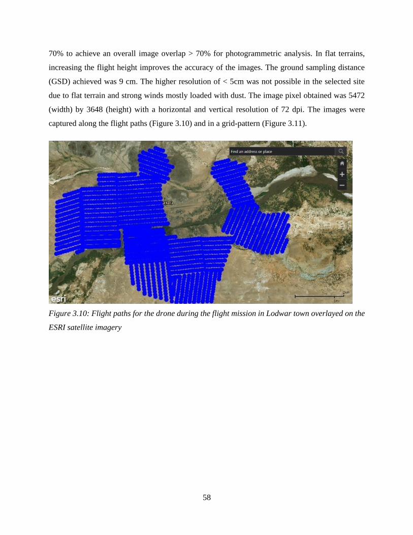
58

70% to achieve an overall image overlap > 70% for photogrammetric analysis. In flat terrains,

increasing the flight height improves the accuracy of the images. The ground sampling distance

(GSD) achieved was 9 cm. The higher resolution of < 5cm was not possible in the selected site

due to flat terrain and strong winds mostly loaded with dust. The image pixel obtained was 5472

(width) by 3648 (height) with a horizontal and vertical resolution of 72 dpi. The images were

captured along the flight paths (Figure 3.10) and in a grid-pattern (Figure 3.11).

Figure 3.10: Flight paths for the drone during the flight mission in Lodwar town overlayed on the

ESRI satellite imagery

59

Figure 3.11: Grid pattern for the image collection points within the boundray of Lodwar town

(c) Vertical electrical sounding

A total of 26 vertical electrical soundings (VES) survey were carried out within the Lodwar

Alluvial Aquifer System to unveil the nature of subsurface geology and to determine the

approximate depth of the aquifer units. The Schlumberger Configuration was used, which involved

passing a current through two electrodes (A and B) to the ground and calculating the potential

difference (V) between the M and N potentials (Figure 3.12). The VES locations within the LAAS

(Figure 3.14) were selected based on a number of factors; the spatial distribution of groundwater

abstraction points, availability of sufficient space for the spread of AB line, and types of overlying

geological formations. The current electrode (AB/2) spacing varied from 1 to 200 m, and the

potential electrode (MN/2) spacing varied from 0.5 to 10 m (Table 3.4). Data were acquired using

PASI 16 GL-N model geophysical equipment. The apparent resistance values were calculated by

multiplying the resistance product by the terametre and the geometric factor, a parameter that

depends on the potential and current electrode spacing. On the log-log graph, the apparent

resistivity values are plotted against the half-current spacing. They were created led by the general

pattern of field curves. Field data were interpreted using IPI2WIN software while the distribution

60

of geoelectric layers in the study area was plotted using Golden Software Surfer Version 16.

Figure 3.12 shows the arrangement of the current and potential electrodes during the fieldwork.

Figure 3.12: Schlumberger array configuration used in the study area

Figure 3.13: Image showing Schlumberger array configuration used during the fieldwork for the

vertical electrical soundings

61

Table 3.4: VES orientation;(east (E), west (W), north (N), south (S), probing depth (m), elevation

(m asl), and length of the AB line at each sounding location of the vertical electrical sounding

(VES)

VES Date Elev. Direction AB VES Date Elev. Direction AB

VES 1 17/02/2019 474 E_W 50 VES 15 04/03/2019 501 NE-SW 200

VES 2_3 18/02/2019 479 E_W 200 VES 16 04/03/2019 492 NE-SW 200

VES 4 18/02/2019 472 NE_SW 200 VES 17 05/03/2019 506 E-W 200

VES 5 19/02/2019 467 EW 200 VES 18 05/03/2019 506 E-W 200

VES 6 19/02/2019 476 NE_SW 200 VES 19 06/03/2019 518 E-W 200

VES 7 20/02/2019 474 NE_SW 200 VES 20 06/03/2019 502 E-W 200

VES 8 25/02/2019 470 NE_SW 200 VES 21 07/03/2019 466 E-W 200

VES 9 25/02/2019 485 E_W 200 VES 22 07/03/2019 462 E_W 200

VES 10 26/02/2019 482 E_W 200 VES 23 08/03/2019 534 E-W 200

VES 11 27/02/2019 466 E-W 200 VES 24 08/03/2019 513 E_W 200

VES 12 27/02/2019 457 E-W 200 VES 25 08/03/2019 495 E_W 200

VES 13 03/03/2019 492 N-S 200 VES 26 09/03/2019 471 E_W 200

VES 14 03/03/2019 494 NE-SW 200 VES 27 09/03/2019 469 E_W 200

Figure 3.14: VES Locations within the Lodwar Alluvial Aquifer System

62

3.4.1.3 Laboratory analyses

a) Petrography

Twelve thin sections for selected rock samples were prepared at the Department of Mines and

Geology, Kenya. The rock samples and the respective sample codes included; nepheline-phonolite

(1650), igneous intrusions (1656 and 3845), conglomerate (3857), sandstone (1659, 3833 and

3858), Augite basalt (1651), Turkana grits (1656 and 3831) and the quartzo-feldspathic gneiss

(3843 and 3844). The thin polished sections were prepared using laboratory techniques described

by Grundmann and Scholz (2015). The petrographic light microscope was used for mineral

identification based on colour, form and other optical properties while observing the thin sections

under plane polarised light (PPL) and crossed polarised light (XPL) (Mugerwa, 2015).

b) X-Ray Fluorescence Spectrometry (XRF)

A total of 54 rock samples were analysed for major and minor trace elements at the International

Council for Research in Agroforestry (ICRAF) lab using X-ray fluorescence technology. Each

rock sample was assigned a specific sample code ranging from 1648-1678 to 3820-3858 for

reconnaissance and detailed fieldworks, respectively. All rock samples were first crushed by the

Department of Mines and Geology, Kenya, before being submitted to the ICRAF laboratory for

XRF analysis. Tracer 5i and vacuum technology were used in quantitative analysis of lighter

elements in rock samples using the XRF technique. The TRACER 5i is flexible with various

applications and incorporates a Silicon Drift Detector (SDD), that offers high-speed data

acquisition and light element sensitivity (Chacha, 2014a). The analytical procedures and quality

control were in accordance with Chacha (2014). The data acquired was filtered using R Knime,

and Shiny App and the filtered data in parts per million (ppm) was then uploaded into the database

for analysis.

c) Atomic Absorption Spectroscopy (AAS)

The determination of major elements in rock samples was done using atomic absorption

spectroscopy (AAS) at the Department of Mines and Geology, Kenya. All the 69 rock samples

obtained during the reconnaissance and during the detailed fieldwork were coded (1647-3858) and

submitted to Mines and Geology labs for analysis. The compounds analysed in the whole rock

analysis include; SiO2, Al2O3, CaO, MgO, Na2O, K2O, TiO2, MnO, Fe2O, and LOI. The

concentrations of these elements are reported as a percentage (%), where the sum should be 100%.

63

However, acceptable totals lie between 98.5 to 101 wt.% (Alhawdar, 2014). The samples were

first crushed to 4µm particle size, and about 0.1 g of the crushed rock sample and 0.6 g of LiBO2

was used to make reagents for analysis. The determination of major rock oxides; silicon (SiO2),

aluminium (Al2O3), calcium (CaO), iron (Fe2O3), sodium Na2O magnesium (MgO),), potassium

(K2O), titanium (TiO2) and manganese (MnO) were carried out using lithium metaborate fusion

procedure designed for analysis of silicates and carbonates (Butler and Kokot, 1971). In this

method, the rock samples are decomposed using lithium metaborate fusion (Butler and Kokot,

1971). Three reagents were used during the analysis; concentrated hydrochloric acid, lanthanum

solution, 5% (w/v) - prepared Standard Conditions for La and Lithium metaborate (LiBO2). The

three reagents help in digestion and extraction of major elements (Belt, 1964; Potts, 1987;

Suvardhan et al., 2003) and to remove chemical interferences (Butler and Kokot, 1971). The

detection limit for most elements is 0.1ppm (Belt, 1964). Replicate analyses determined the

precision and accuracy of this method through actual separate digestions and subsequent

quantification. The nitrous oxide-acetylene flame prevented inter-element interferences.

Each element weight was calculated as follows;

𝐸𝑙𝑒𝑚𝑒𝑛𝑡 (𝑤𝑡 %) =(𝑁𝑜. 𝑜𝑓 𝑔𝑟𝑎𝑚𝑠 𝑖𝑛 𝑠𝑜𝑙𝑢𝑡𝑖𝑜𝑛∗(𝑑.𝑓)∗0.02)

𝑤𝑒𝑖𝑔ℎ𝑡 𝑜𝑓 𝑡ℎ𝑒 𝑠𝑎𝑚𝑝𝑙𝑒 Equation 3-5

where d.f. = dilution factor

3.4.1.4 Data analysis

a) Vertical electrical sounding

The field data were interpreted using IPI2WIN software. All the 26 vertical electrical soundings

field data were entered into an excel spreadsheet and later imported to the IPI2WIN software

interface. At the initial opening of the data file, a graph is displayed without the resistivity cross-

section (Kurniawan, 2009). The best-fitting two-layered model is selected as recommended by

IPI2WIN software. The software automatically will suggest a best-fitting model for the initial

interpretation of the input sounding points data (Gurugnanam et al., 2009). Model editing entails

changing the number of layers by splitting or joining them (to add or remove a layer) and changing

the properties of the layers. The fitting error (Error = 1.92 % to 3.69) expresses the degree of

uncertainty in the computed model parameters and the goodness of fit in the curve fitting algorithm

64

(Kurniawan, 2009). Several inversions are used to reproduce the resistivity of different layers and

the corresponding thickness until the model parameters of all the VES curves are completely

resolved with the fitting error (Kurniawan, 2009). The resistivity layer, log resistivity graph,

resistivity depth table, and pseudo-cross-section are the results of sounding data analysis using

IP2Win software, and they can all be exported in preferred file formats. The benefit of IPI2Win

software is that it uses 2D cross-sections (many subsurface layers) to identify the targeted aquifer.

The only shortcoming in the IP2Win software is a bug that occurs frequently when analyzing data

and can be fixed by restarting the software.

b) Drone image processing

Drone-acquired images are processed using photogrammetry techniques. Several

photogrammetric software exists; Burnham (2019) has evaluated the various software based on

their market price, quality of products and nature of projects. Pix4D software was selected due to

its robust capability to process huge number of images and the high quality of outputs (Burnham,

2019). The 2039 drone acquired images were processed using PiX4D photogrammetric software

that uses Structure-from-Motion (SfM) algorithms. The SfM is a photogrammetric technique that

can generate 3-dimensional (3-D) information from 2-dimensional photos. The process involves

the identification of key points such as rock outcrops, trees, and fractures between overlapping

images and utilizes triangulation calculations to determine the 3-D location for the set of data

points (point clouds). Each point within the point cloud has unique coordinates (latitude, longitude,

and elevation) that allow for post GIS analysis and interpretation. The outputs from the drone-

acquired images include high-resolution orthomosaics (geometrically corrected for distortions), a

high-resolution digital terrain model, and a textured 3-D mesh. The workflow and outputs of image

processing using the Pix4D software are shown in Figure 3.15.

65

Figure 3.15: Workflow for processing drone-acquired images using Pix4D photogrammetric

software (Hawkins, 2016)

c) Determination of aquifer characteristics

The aquifer characteristics determined are outlined below.

(i) Porosity

Porosity is expressed as;

𝑃𝑜𝑠𝑜𝑠𝑖𝑡𝑦 (𝑛) =𝑉𝑣

𝑉 Equation 3-6

Where Vv is the volume of voids in a porous medium, while V is the

total volume of the porous medium

Generally, consolidated materials have lower porosities than unconsolidated materials – gravels,

sands, and silts with angular and rounded particles have lower porosities as compared to clay.

Besides, the poorly sorted sub-surface materials have lower porosities than well-sorted sub-surface

deposits.

(ii) Specific yield

The specific yield (Sy) expressed as;

66

𝑆𝑦 =𝑉𝑑

𝑉 Equation 3-7

Where, Vd is the volume of water drained by gravity, and V is the total volume of the porous

medium. Porosity can be linked to specific yield by;

𝑛 = 𝑆𝑦 + 𝑆𝑟 Equation 3-8

Where n = porosity, Sy= specific yield and Sr = specific retention

Specific yield is dimensionless and often depends on the grain size, distribution and shape of pores,

subsurface compaction, and duration of drainage. Due to compaction processes, the value of

Sy decreases with depth. Typical porosity values and specific yield for different geological

materials are given in Table 6 (Brassington, 2010).

Table 3.5: Representative values of porosity and specific yield for different geological materials

(Brassington, 2010)

No Type of Geological Material Porosity (%) Specific Yield

(%)

1 Medium Gravel 32.00 24.00

2 Fine Gravel 34.00 25.00

3 Coarse Sand 39.00 27.00

4 Medium Sand 39.00 28.00

5 Fine Sand 43.00 23.00

6 Silt 46.00 8.00

7 Clay 42.00 3.00

8 Fine-grained Sandstone 33.00 21.00

9 Medium-grained Sandstone 37.00 27.00

10 Limestone 30.00 14.00

11 Dune Sand 45.00 38.00

12 Loess 49.00 18.00

13 Peat 92.00 44.00

14 Schist 38.00 26.00

15 Siltstone 35.00 12.00

16 Till (mainly Sand) 31.00 16.00

17 Till (mainly Silt) 34.00 6.00

18 Tuff 41.00 21.00

67

(iii) Storage coefficient and specific storage

Storage coefficient is a dimensionless property of an aquifer is expressed as;

𝑆 = 𝑆𝑠 + 𝑏 Equation 3-9

Where Ss= specific storage and b= thickness of the aquifer material.

The specific storage is a dimension of [L-1] and is expressed as;

𝑆𝑠 = 𝜌𝑤𝑔 (𝛼 + 𝑛𝛽) = 𝑦𝑤 (𝛼 + 𝑛𝛽) Equation 3-10

Where ρw denotes the density of water; α denotes compressibility of the aquifer material and (is

equal to 1

𝐸𝑠, Wherein Es is the bulk modulus of elasticity of aquifer skeleton); β = compressibility

of water and ( is equal to 1/Kw, wherein Kw is the bulk modulus of elasticity of water), n = porosity

of the aquifer material, and γw refers to the unit weight of water. Therefore, the specific storage is

the most crucial aquifer parameter depending on the type of aquifer material, the amount of water

contained in the aquifer, and the overburden stress. The value of Kw is 2.1 x 109 N/m2, while the

Es values for selected geological materials are shown in Table 3.4 (Raghunath, 2007).

Since the storage coefficient (S) of an aquifer is a function of aquifer thickness and is different for

every location. The storage coefficient (S) of an aquifer can be expressed as;

𝑆 = 𝑦𝑤 (𝛼 + 𝑛𝛽) 𝑥 𝑏 Equation 3-11

The study of Mook (2000) determined the values of S for confined and unconfined aquifers. The

value of S in the confined aquifer ranged from 5 x 10-5 to 5 x 10-3 indicating substantial pressure

changes over extensive areas required for sufficient yields (Mook, 2000). The storage coefficient

(S) of unconfined aquifers, on the other hand, was equal to the effective porosity because most of

the groundwater is released by a declining unconfined (free) water table because of gravitational

drainage. S ranges from 0.15 to 0.25 in unconfined aquifers of alluvial sediments, which is much

higher than in confined aquifers (Mook, 2000).

(iv) Transmissivity (T)

Transmissivity of an aquifer is expressed as;

68

𝑇 = 𝐾𝑏 (𝑚2/𝑑𝑎𝑦) Equation 3-12

Where T = transmissivity, K = hydraulic conductivity, b = saturated aquifer thickness

(v) Hydraulic Conductivity

In Darcy's law, hydraulic conductivity (K) acts as a constant of proportionality relating the specific

discharge of a porous medium under hydraulic gradient expressed as;

𝑣 = −𝐾𝑖 Equation 3-13

Where v = specific discharge, K = hydraulic conductivity and i = is hydraulic gradient.

Table 3.6: Typical values of hydraulic conductivity in various geological materials

No. Materials Hydraulic Conductivity (m/s)

Min Ma x

1 Fine Sand 2.0 x 10-7 2.0 x 10-4

2 Medium Sand 9.0 x 10-7 5.0 x 10-4

3 Coarse Sand 9.0 x 10-7 6.0 x 10-3

4 Sand; Clean; Good Aquifer 1.0 x 10-5 1.0 x 10-2

5 Sand/Gravelly Sand; Poorly Graded; Little to No Fines 2.5 x 10-5 5.3 x 10-4

6 Sand/Gravelly Sand; Well Graded; Little to No Fines 1.0 x 10-8 1.0 x 10-6

7 Silty Sand 1.0 x 10-8 5.0 x 10-6

8 Clayey Sand 5.5 x 10-9 5.5 x 10-6

9 Alluvial Gravel/Sand 4.0 x 10-4 4.0 x 10-3

10 Sand/Gravel; Uniform 4.0 x 10-3 4.0 x 10-1

11 Sand/Gravel; Well Graded; No fines 4.0 x 10-5 4.0 x 10-3

12 Gravel 3.0 x 10-4 3.0 x 10-2

13 Silty Gravel/Silty Sandy Gravel 5.0 x 10-8 5.0 x 10-6

14 Silt; Compacted 7.0 x 10-10 7.0 x 10-8

15 Clay 1.0 x 10-11 4.7 x 10-9

16 Limestone / Dolomite 1.0 x 10-9 6.0 x 10-6

17 Sandstone 3.0 x 10-10 6.0 x 10-6

18 Siltstone 1.0 x 10-11 1.4 x 10-8

19 Anhydrite 4.0 x 10-13 2.0 x 10-8

20 Permeable Basalt 4.0 x 10-7 2.0 x 10-2

21 Igneous/Metamorphic Rock; Fractured 8.0 x 10-9 3.0 x 10-4

22 Basalt 2.0 x 10-11 4.2 x 10-7

23 Igneous/Metamorphic Rock; Unfractured 3.0 x 10-14 2.0 x 10-10

69

Hydrogeochemistry and Aquifer Susceptibility to Pollution

Methods described herein are for investigation of the hydrogeochemistry of the LAAS and its

susceptibility to pollution. Each method and the fieldwork procedures are presented, and the

analytical rationale is provided in Appendix 3-2

3.4.2.1 Desktop studies

Secondary data on water quality were very limited. Available data was collected from Water

Resources Authority (WRA) for the period 2015 and 2017 for five boreholes (LOWASCO Bh,

Nakwameki Bh, Kakemera Bh, Napuu Church, and Napuu Mission) and one Turkwel River

sample. The datasets contained the following parameters: electrical conductivity, pH, total

suspended solutes, turbidity, total dissolved solids, total hardness, total alkalinity (EC), iron (Fe2+),

manganese (Mn2+), magnesium (Mg2+), calcium (Ca2+), fluoride, chloride (Cl-), sulphate (SO42-),

Nitrite (NO2-) and nitrate (NO3

-). From the desk study review, it was clear that understanding of

water quality and hydrogeochemistry of the LAAS required a detailed water sampling framework

that included water sampling from every possible groundwater source as well as seasonal water

quality monitoring of selected wells.

3.4.2.2 Fieldwork

Seasonal water sampling was carried out in the study area as follows; in the dry season of February

2018 water samples collected included; seven samples of the Turkwel River, ten borehole samples

and two handpump samples. May 2018 was the wet season in the area, and extensive water point

mapping and groundwater sampling were conducted. As a result, a total of 137 groundwater

sources were established in the region (53 boreholes, 84 handpumps). Of these, only 94 water

points (53 handpumps and 41 boreholes) were sampled, an equivalent of 68.61 per cent. The rest

47 (31 Hps and 16 Bhs), were not sampled because they were either dry, vandalized, or were non-

operational at the time of the survey. In the subsequent dry season, February 2019, a total of 58

groundwater samples (27 boreholes and 31 handpumps) of the previous 94 set were collected.

Figure 15 shows the location of the surface water and groundwater samples (Figure 3.16).

Duplicate samples were collected from each sampling site for cation and anion determinations,

respectively, as well as for isotope analysis. As sampling containers, clean polythene 500 mL

bottles with air-tight caps were used, and each bottle was cleaned with deionized water before

sampling. To preserve the cation samples, three drops of analytical grade % nitric acid were used.

70

Before being placed in a cool box for transport to Nairobi, the bottles were labeled and refrigerated

at 4 °C in the laboratory. The pH, Electrical conductivity, and temperature were measured in the

field using hand-held Combo Tester HI98129 for all the water samples. EC was measured in the

groundwater samples and expressed in milliSiemens per centimetre (µS/cm).

Figure 3.16: Surface water and groundwater sources in the mid-Turkwel River watershed

3.4.2.3 Laboratory analysis of water samples

All the samples were submitted to the Water Resources Authority Central Lab for full chemical

analyses. The laboratory analyses were based on standard analytical procedures (APHA, 1985).

The measured parameters include; pH, turbidity, total hardness, total alkalinity, EC, Ca, Mg, Na,

K, Fe, Mn, Cl, F, NO3, NO2, HCO3, SO4, and CO3. The standard laboratory tests for the various

parameters are discussed below.

Turbidity was determined using a turbidimeter MRC model in nephelometric turbidity units

(NTU), where 5 NTU is the guideline value established by both WHO (2011) and KEBS (2014).

Hardness was determined using the titrimetric method that measures the calcium and magnesium

71

ions, and the results were expressed in CaCO3/l. The guideline value provided by WHO for total

hardness in natural portable water is 500 mg/L, while that of KEBS is 600 mg/L. The WHO

guideline value of 500 mg/L was used for drinking water evaluation since it is lower than that of

KEBS. Total alkalinity was measured using the titrimetric method. The guideline value of 500

mg/L established by both WHO (2011) and KEBS (2014) was used to evaluate the total alkalinity

in groundwater.

The major cations analysed were sodium, potassium, calcium, magnesium, iron, and manganese,

using standard analytical procedures based on APHA (1995). Sodium and potassium were

determined using the Jenway PFP7 photometer standard flame photometric method. The results

were expressed in mg/L, and the guideline values of 200 mg/L (sodium) and 50 mg/L (potassium)

were used to evaluate their concentrations in groundwater. Calcium and magnesium were

determined using titrimetric methods, where the calculation method was used to determine

magnesium concertation. The results were expressed in mg/L, and a guideline value of 100 mg/L

established by WHO (2011) for calcium and magnesium was used to evaluate the drinking water

quality. In this case, the guideline value of 150 mg/L defined by KEBS (2014) for calcium was

ignored. The iron was determined using a colorimetric method, while the manganese was

determined using the Jenway Calorimeter 6051 and the Phenanthroline Perusalfate method. The

persulfate method is the most used colorimetric method for measuring manganese because the use

of mercuric ion controls interference from a constrained chloride ion concentration. The

measurements were in milligrams per litre, with a guideline value of 0.3 mg/L for Fe2+ and 0.1

mg/L for Mn2+ used for drinking water evaluation.

Chloride was measured using the argentometric method, and this method is often used in relatively

clear waters and when 0.15 to 10 mg of Cl- is present in the portion titrated. Fluoride was

determined using the ion-selective electrode method using a Jenway 3345 model using Ion Meter.

The results for both chloride and fluoride were expressed in mg/L. The WHO and KEBS have

established guideline values of 250 mg/L for Cl- and 1.5 mg/L for F- and were used to evaluate the

drinking water quality. Nitrate was determined using the UV spectrophotometric method by

utilizing UVmini 1240 Shimadzu spectrophotometer. Nitrite was, on the other hand, determined

using the colorimetric method using the Jenway Calorimeter 6051 model. The results for both

nitrate and nitrite were expressed as mg/L (NO3-N) and mg/L (NO2-N), respectively. The WHO

and KEBS guideline value for NO3- in drinking water is 10 mg/L (NO3-N). The WHO guideline

72

value for NO2- is 0.1 mg/L (NO2-N) while that of KEBS is 0.003 mg/L (NO2-N). For nitrite, the

WHO (2011) guideline value was used for drinking water evaluation since it is also used by the

United States Environmental Protection Agency (EPA, 2018). Sulphate was determined using the

turbidimetric method, and the results were expressed in mg/L while the free carbon dioxide was

measured using the trimetric method, and the results were also expressed in mg/L. The WHO

(2011) guideline value for SO42- is 450 mg/L while that of KEBS (2014) is 400 mg/L, and the

KEBS value was used for drinking water evaluation. No guideline value has been provided for

free carbon dioxide.

3.4.2.4 Data analysis

a) Data validation

Validation of the chemical data obtained from the Central Laboratory of the Water Resources

Authority was carried out by calculating the charge balance of all surface water and groundwater

samples. Charge balance determination involved four key stages, where all the calculations were

carried out in an Excel spreadsheet.

Step 1: The concentration of each cation and anions were divided by their respective atomic masses

and molecular masses to obtain the milli-equivalents. The cations tested were Ca2+, Mg2+, Na+, K+,

Fe2+, and Mn2+, while the anions were HCO3-, CO3, SO4

2-, Cl-, F-, NO2- and NO3

-.

The atomic masses and oxidation states used for cations and anions are shown in Table 3.7.

Table 3.7: Atomic masses and oxidation states of cations and anions tested

cations Atomic mass oxidation state Anions Molecular mass Oxidation state

Ca 40.00 2 HCO3 61.02 -1

Mg 24.30 2 CO3 60.00 -2

Na 23.00 1 SO4 96.00 -2

K 39.00 1 Cl 35.50 -1

Fe 55.80 2 F 19.00 -1

Mn 54.90 2 NO3 62.00 -1

Step 2: The mEq calculation was determined for cations and anions by multiplying the result in

step 1 above with the respective valence electrons or the oxidation state.

73

Step 3: Total cations and total anions were determined in Excel by obtaining the sum of cations

and anions from step 2 above.

Step 4: The overall charge balance was determined using the equation:

𝐶ℎ𝑎𝑟𝑔𝑒 𝑏𝑎𝑙𝑎𝑛𝑐𝑒 =(Ʃ𝑐𝑎𝑡𝑖𝑜𝑛𝑠−Ʃ𝑎𝑛𝑖𝑜𝑛𝑠)

(Ʃ𝑐𝑎𝑡𝑖𝑜𝑛𝑠+Ʃ𝑎𝑛𝑖𝑜𝑛𝑠)∗ 100 Equation 3-14

Generally, accepted limits of experimental error are a charge balance of ± 5 % (Huh et al., 1998),

and the excess charge is attributed to unanalysed organic acid anions or the analysed cations and

anions present in the water sample. According to Huh et al. (1998), the causes of charge imbalance

include: laboratory error, missed sampling procedure, use of unfiltered water samples and the

number of parameters measured. Unfiltered water samples may contain particulate matter that

dissolves into the sample when an acid preservative is added. Following the charge balance

determination, the chemical data were then used to evaluate the drinking water quality, seasonal

water quality variation, identification of hydrochemical facies, and determining the aquifer

hydrogeochemistry.

b) Determination of drinking water quality

Field and Laboratory results for all physico-chemical parameters were compared against the

guideline values provided by WHO (2011) and KEBS (2014). Based on WHO (2011), each

country should use its own standards for drinking water following public health policies and

practices. In this study, KEBS guideline values were used whenever the value was similar or lower

than that of the WHO, whereas the guideline values of the WHO (2011) were applied in case of

higher KEBS values (2014) like in the case of calcium.

c) Water quality index determination

Samples were assessed for 13 physicochemical parameters that included pH, EC, Ca2+, Mg 2+, Na+,

K+, Fe2+, Mn2+, HCO3, SO42-, Cl-, F-, and NO3

- to assess the suitability of groundwater for drinking

and determine the degree of aquifer contamination. The water quality index was determined using

Equation 3-10 above for the Weight Arithmetic water quality index (WQI). Rating weights (wi)

ranging from one to five were assigned to the selected parameters based on their overall influence

on water quality (Ravikumar et al., 2013; Kumari et al., 2014; Boah et al., 2015). Table 3.8 below

shows the rating weights and unit weights assigned to each parameter to calculate the water quality

index. Water quality index results of the study are then expressed in terms of excellent quality (0-

74

25), good quality (26-50), poor quality (51-75), very poor quality (76-100), unsuitable for drinking

(WQI > 100). A spatial map was then plotted using Surfer software from the resultant water quality

indices to yield water quality index map for the study area.

Table 3.8: The rating weights (wi) and unit weight (Wi) assigned to the water quality parameters

Parameter WHO/ KEBS

Rating (wi)

Unit weight (Wi)

pH 8.5 4 0.098

EC 1500 4 0.098

Ca 100 2 0.049

Mg 100 2 0.049

Na 200 3 0.073

K 50 1 0.024

Fe 0.3 3 0.073

Mn 0.1 5 0.122

HCO3 500 3 0.073

SO4 400 3 0.073

Cl 250 3 0.073

F 1.5 5 0.122

NO3 10 3 0.073

n=13 ∑wi = 41 ∑Wi = 1.001

The primary goal of water quality monitoring is to determine suitability for a specific use. The

water quality index (WQI) is a mathematical tool used to convert large amounts of water quality

data into a single number that represents the level of water quality (Ravikumar et al., 2013; Sharma

and Chhipa, 2016). Generating WQI in a specific area is a critical step in land use planning and

sustainable water resource management (Kumar and James, 2013; Stambuk-Giljanovic, 1999;

Yidana et al., 2010). The water quality index is widely regarded as the most effective tool for

communicating water quality trends to the public and policymakers (Kumari et al., 2014). A water

quality index condenses large amounts of water quality data into simple terms such as excellent,

suitable, or unsuitable for drinking (Boah et al., 2015). The weighted arithmetic index method was

used to calculate the water quality index (WQI), which reflects the influence of water quality

parameters on overall water quality (Ravikumar et al., 2015).

The WQI is calculated as follows;

75

𝑊𝑄𝐼 =∑ 𝑞𝑖𝑤𝑖𝑛

𝑖=1

∑ 𝑤𝑖𝑛𝑖=1

Equation 3-15

Where,

qi = quality rating of each water quality parameter

wi = unit weight if each water quality parameter.

In order to calculate the WQI, each of the 15 selected parameters was assigned weights (wi)

ranging from 1-5 based on their relative importance in overall drinking water quality (Boah et al.,

2015; Sharma and Chhipa, 2016; Javadi et al., 2017; Faye et al., 2019). Secondly, the relative

weight (Wi) of each parameter was calculated using the equation;

𝑊𝑖 =𝑤𝑖

∑ 𝑤𝑖𝑛𝑖=1

Equation 3-16

where,

Wi = relative weight

wi = weight of each parameter and

n = is the number of parameters

Thirdly, the quality rating qi was obtained by dividing the observed concentration of parameter in

each sample by the respective standard based on KEBS guidelines using the equation:

𝑞𝑖 = (𝐶𝑖

𝑆𝑖) ∗ 100 Equation 3-17

Where,

qi = quality rating

Ci = observed concentration of each parameter

Si = KEBS drinking water standard for each physic-chemical parameter

For calculating the WQI, the water quality sub-index (SI) was first determined for each chemical

parameter by:

76

𝑆𝐼 = 𝑤𝑖 ∗ 𝑞𝑖 Equation 3-18

Finally, the WQI was determined as follows;

WQI = ∑SI 1-n Equation 3-19

The water samples were then rated based WQI calculation (Richards, 1954; Boah et al., 2015;

Sharma and Chhipa, 2016) in Table 3.9.

Table 3.9: Water quality rating based on WQI

WQI Water Quality Rating

0-25 Excellent

26-50 Good

51-75 Poor

76-100 Very poor

>100 Unsuitable for drinking

d) Spatial maps

Spatial maps for physico-chemical parameters were prepared for the study area using Golden

Software Surfer V16, where the Kriging method was applied for gridding. When estimating values

in unknown areas, kriging is a geostatistical interpolation technique that takes both distance and

degree of variation between known data points into account (Wackernagel, 2013) and thus,

considered the most accurate gridding method for most datasets.

e) Determination of hydrochemical facies

There are numerous graphical methods for representing water chemistry and hydrochemical facies

(Giménez-Forcada, 2010). Triangle diagrams depict concentrations of major cations and anions as

a percentage meq/L of total anions and cations, with a point representing different chemical

compositions assigned to different positions in each triangle (Ghoraba and Khan, 2013; Glover et

al., 2012). The majority of the hydrochemical studies use piper trilinear diagrams (Glover et al.,

2012; Kumar, 2013; Lokhande and Mujawar, 2016; Ravikumar et al., 2015) to represent the

groundwater facies. The Piper diagram's limitation is that a single point not only represents unique

facies, but the point also takes on the corresponding interpretation (Giménez-Forcada, 2010).

77

According to Giménez-Forcada (2010), the representation of two ions in the same field of the Piper

diagram implies a similar behaviour of both water types and reinforces the value of a parameter in

the interpretation of a process.

The hydrochemical facies of the groundwater and surface water samples were determined using

Piper trilinear diagram (Kumar, 2013). The sample plots fall in different areas in these diagrams,

characterising the different facies (Afzali et al., 2015; Glover et al., 2012). The anions and anions

are expressed in Meq/L in the Piper plot. Anions are plotted in the left triangle, while cations are

plotted as a single plot in the right triangle. The tri-linear diagram's central diamond-shaped area

is a projection of these two plots (Ghaffar et al., 2017) (Ghaffar et al., 2017). Groundwater charts

can more effectively express similarities and differences in groundwater samples because similar

qualities of samples are plotted together to form groups (Abdelshafy et al., 2019).

f) Rock-water interactions

(i) Mineral saturation indices

The geochemical modelling tools used to calculate saturation indices of water include WATEQF,

SOLMNEQ, and PHREEQC (Haile-Meskale, 2017). This study used the PHREEQC tool to

evaluate the groundwater of the area. The saturation indexes were determined on the groundwater

samples of the study area utilizing the PHREEQC – hydrogeochemical equilibrium model for

windows (Haile-Meskale, 2017).

The mineral saturation index helps to determine the equilibrium state of water for a mineral phase

using analytical data (Aghazadeh et al., 2017; Garrels and Berner, 1983). Changes in the saturation

state are used to identify the geochemical reactions controlling the water chemistry and to

differentiate between different stages of hydrochemical evolution (Aghazadeh et al., 2017; Al-

Ruwaih, 2017). The saturation index (SI) is given by (Garrels and Mackenzie 1967);

𝑆𝐼 = 𝐿𝑜𝑔𝐼𝐴𝑃

𝐾𝑇 Equation 3-20

Where IAP indicates the ion activity product of the dissociated chemical species in solution, and

KT denotes the chemical's equilibrium solubility product at the sample temperature (Garrels and

Mackenzie 1967).

78

As saturation indices, positive and negative saturation indices can be obtained (Zaheeruddin and

Khurshid, 2004). Positive SI indicates that the groundwater is oversaturated for a specific mineral,

unable to dissolve more of the mineral, whereas negative SI indicates that the groundwater is

under-saturated for a specific mineral (Aghazadeh et al., 2017; Al-Ruwaih, 2017). SI values close

to zero indicate that groundwater and the mineral are in equilibrium. Groundwater discharged from

an aquifer containing a sufficient amount of the mineral with sufficient resident time to reach

equilibrium results in zero index values (Aghazadeh et al., 2017).

(ii) Principal component analysis (PCA) and Cluster hierarchical analysis (HCA)

Multivariate statistical techniques are widely used to evaluate groundwater chemistry and to

determine prevailing aquifer processes (Dash et al., 2018; Abdullahi et al., 2014; Islam et al.,

2017). Principal Component Analysis (PCA) and Hierarchical Cluster Analysis (HCA) are the

most used statistical methods for determining the most important contributing parameters that

decide the geochemistry of groundwater samples (Li et al., 2018). PCA is useful for identifying

correlated variables as well as the process and grouping of types of water quality (Mrklas et al.,

2006; Wu et al., 2015). HCA, on the other hand, groups similar observations together to reveal

different chemical characteristics of the various groups of groundwater samples (Dash et al., 2018;

Abdullahi et al., 2014; Islam et al., 2017). Statistical Package for Social Sciences (SPSS) and

Microsoft Excel Add-in, XLSTAT, are the widely used software for PCA and HCA analytical

tools (Dash et al., 2018; Douglas, 2015; Abdullahi et al., 2014).

Both PCA and HCA were applied to the 94 groundwater samples from boreholes (41), and

handpumps (53) collected in the wet season (May 2018), and 58 samples collected in the dry

season. The physico-chemical parameters for all samples were; pH, EC, TDS, Ca, Mg, Na, K, Fe,

Mn, HCO3, CO3, SO4, Cl, F, NO3. PCA and HCA were performed on groundwater samples using

group average clustering and Euclidean distance methods based on dissimilarities (Islam et al.,

2017; Ravikumar and Somashekar, 2015). The extraction methods of varimax rotation and Keiser

normalization were applied in the PCA to interpret the geochemical data (Ravikumar and

Somashekar, 2015) and the resultant Principal Components (PCs) with eigenvalues >1 was

retained (Cattell and Jaspers 1967 Ravikumar and Somashekar, 2015; Islam et al., 2017). In the

case of HCA, Ward's linkage clustering method was used for distance computing (Glover et al.,

2012; Li et al., 2018), which is considered more accurate than, complete linkage, single linkage,

79

and average linkage methods (Li et al., 2018). Ward's method employs the nearest-neighbour chain

algorithm to determine the best merging cluster pair that produces the most distinct signature for

hydrogeochemical clusters in water samples (Li et al., 2018). Using discriminant function analysis,

the significance of seasonal variations in water chemistry was determined.

g) Identification of point and non-point pollution sources

Point sources of pollution refer to the discharge of contaminants into the groundwater through a

pipe, ditch, discrete fissure, tunnels, concentrated animal feed, and municipal wastewater

(Abdullahi et al., 2014; Islam et al., 2017) while nonpoint sources may result from agricultural

chemicals (fertilizers and pesticides) through surface runoff, precipitation, atmospheric deposition,

seepage, drainage, or hydrological modification (Islam et al., 2017). Sound management of non-

point sources of pollution groundwater requires a thorough scientific understanding of these

sources and the linkages between nonpoint sources and groundwater discharges to users or affected

well and streams (Lathamani et al., 2015). The likely point sources within the study area include;

on-site septic systems, municipal wastes, and industrial chemicals, while the potential non-point

sources may include upstream use of agricultural chemicals. The concentration of nitrates and

sulphates in groundwater are used to indicate point and non-point pollution sources, respectively

(Bruthans et al., 2019; Gardner and Vogel, 2005; Miljević et al., 2012).

To identify the point and non-point pollution sources, the water quality index map of the area was

also overlaid on the DEM to evaluate the potential areas of point pollution sources. The drone-

acquired digital terrain model (DEM), with a resolution of 1.26 m for the Lodwar municipality,

was used to extract the stream lineament within the municipal boundary. It was also used to

determine possible dispersal routes of non-point sources facilitated by stream channels. Heat maps

of SO4 and NO3 in boreholes and handpumps were overlaid on DEM for the Lodwar municipality

to identify whether they originated from the point or non-point sources and to establish the extent

of anthropogenic pollution. Boreholes and handpumps located on one or more streams are likely

to bear non-point source pollution while those located away from stream lineament are polluted

by point sources (Barilari et al., 2020).

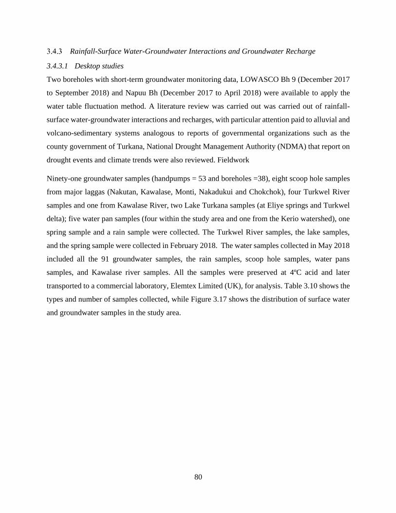
80

Rainfall-Surface Water-Groundwater Interactions and Groundwater Recharge

3.4.3.1 Desktop studies

Two boreholes with short-term groundwater monitoring data, LOWASCO Bh 9 (December 2017

to September 2018) and Napuu Bh (December 2017 to April 2018) were available to apply the

water table fluctuation method. A literature review was carried out was carried out of rainfall-

surface water-groundwater interactions and recharges, with particular attention paid to alluvial and

volcano-sedimentary systems analogous to reports of governmental organizations such as the

county government of Turkana, National Drought Management Authority (NDMA) that report on

drought events and climate trends were also reviewed. Fieldwork

Ninety-one groundwater samples (handpumps = 53 and boreholes =38), eight scoop hole samples

from major laggas (Nakutan, Kawalase, Monti, Nakadukui and Chokchok), four Turkwel River

samples and one from Kawalase River, two Lake Turkana samples (at Eliye springs and Turkwel

delta); five water pan samples (four within the study area and one from the Kerio watershed), one

spring sample and a rain sample were collected. The Turkwel River samples, the lake samples,

and the spring sample were collected in February 2018. The water samples collected in May 2018

included all the 91 groundwater samples, the rain samples, scoop hole samples, water pans

samples, and Kawalase river samples. All the samples were preserved at 4ºC acid and later

transported to a commercial laboratory, Elemtex Limited (UK), for analysis. Table 3.10 shows the

types and number of samples collected, while Figure 3.17 shows the distribution of surface water

and groundwater samples in the study area.

81

Table 3.10: Samples submitted for stable isotope analysis at Elemtex lab, United Kingdom

No Sample type Number of samples tested for 18O

Number of samples tested for 2H

Number of samples tested for 3H

1 Rain 1 1 1

2 Turkwel River 5 5 1

3 Kawalase River 1 1 0

4 Scoop Holes 4 4 0

5 Water pans 5 5 0

6 Handpumps 52 52 26

7 Boreholes 38 38 13

8 Spring 1 1 0

9 Lake 2 2 2

Total 110 110 43

82

Figure 3.17: Distribution of surface water and groundwater isotope samples within the mid-

Turkwel watershed

3.4.3.2 Laboratory analyses

a) Oxygen and Deuterium Measurements

The measurement of hydrogen (2H) and oxygen (18O) isotope ratios in water samples was done

using an isotope ratio mass spectrometer (IRMS) combined with a high-temperature conversion

elemental analyser (TC/EA) operated in continuous flow (CF) mode. The isothermal

chromatography, which is part of TC/EA, separates the reaction gasses and these gasses are

admitted to the IRMS via the ConFlo IV universal interface, where oxygen and hydrogen gases

are converted to CO and H2 respectively (Yeh and Lee, 2018). The ConFlo IV allows for automatic

sample gas dilution and generation of reference gas pulses, enabling for the individual referencing

of each sample gas peak (Carter and Barwick, 2011; Yeh and Lee, 2018) (Figure 3.18).

83

Standard CO2 with known δ18O values were reacted with the water samples during pre-treatment

for two hours to achieve an equilibrium. Excess water was removed by freezing and purification,

where the CO2 produced was collected in a glass tube. The IRMS was utilized to evaluate the

isotopic oxygen compositions of water samples that had attained equilibrium with oxygen in the

CO2. The hydrogen was extracted using zinc granules to produce H2, where 200 mL of zing

granules were weighed, and a capillary tube was then used to remove 4 µL of the water sample.

Both the zinc granules and the water sample were sealed in a 6.35 mm vacuum Pyrex specimen

and placed in a 1400 °C oven for 30 minutes to allow for the water sample to completely react

with zinc to produce H2 by reduction process (Carter and Barwick, 2011). The specimen tube was

then placed in the IRMS equipment to quantify the hydrogen isotopic composition. For quality

control, five samples were injected at a time, and the normalization followed the requirements of

FIRMS IRMS guide v2 (Carter and Barwick, 2011). The isotope ratios were expressed as δ2H and

δ18O values relative to the Vienna Standard Mean Ocean Water (VSMOW) reference materials

where δD = 0 ‰ and δ18O = 0 ‰ (Carter and Barwick, 2011). In this study, the analytical

reproducibility was ±0.1 for the oxygen and ± 1.0 for deuterium.

Figure 3.18: Simple schematic diagram of TC/EA-IRMS for determination of δ2H and δ18O

84

b) Tritium measurement

Tritium analysis was carried for 43 water samples consisting of 26 handpumps, 13 boreholes, two

lake samples, and one sample each for rainfall and Turkwel river samples. Tritium was measured

by a liquid scintillation counter (LSC) (Motzer, 2007) by counting β- decay events. A 10 ml sample

of distilled and electrolytically enriched water was mixed with the scintillation compound, which

emits a photon when struck by a - particle. Using Spectrometer 1220 Quantulus equipment,

photomultiplier tubes in the scintillation counter convert photons to electrical pulses that are

counted over 90-minute intervals of six cycles (Moore, 2011). The count obtained was compared

to calibrated standards and blanks to calculate the results. Increased precision was obtained by

electrolytic enrichment of 3H in water prior to counting. Direct liquid scintillation counting carries

an accuracy of ± 8 TU, but with enrichment and LSC, this is improved to ± 0.8 TU (Singh et al.,

2016). Propane synthesis was carried out to improve the analytical precision to ± 0.1 TU (Moore,

2011).

3.4.3.3 Data analysis

a) Recharge estimation using 2H and 18O isotopes

The oxygen and hydrogen isotopic compositions of precipitation and groundwater can be used to

assess groundwater recharge mechanisms (Adomako et al., 2010; Yeh et al., 2014). In this study,

the isotopes for the groundwater samples were also compared to that of the surface water in the

area. The Global Network of Isotopes in Precipitation (GNIP) provides long term d-excess data

across the globe, which is used to characterize the evolution of water through the hydrologic

cycle (Bershaw et al., 2018). The GNIP data were download from https://nucleus.iaea.org, three

GNIP monitoring stations within the proximity of the study area; Moyale, Kericho, and Soroti

(Uganda). Kericho station had a total of 19 observations, Soroti had 14, and Moyale station had

only four observations. Kericho and Soroti GNIP stations are in high altitude regions while the

Moyale station is in a low altitude region, thus, exhibiting varying isotopic compositions in the

rainfall.

The Global Meteoric Water Line (GMWL) was produced for each of the three stations using the

equation δD = 8 * δ18O + 10 (Craig, 1961). The Local Meteoric Water Lines (LMWL) for each

station was plotted based on the relationship between isotopic compositions of hydrogen and

oxygen in precipitation (Oiro et al., 2018). The GMWL based on Crag’s model and the trend line

85

analysis of the LMWL was used as the reference for the stable groundwater isotopes of the study

area. By associating the analysed stable isotopes with the derived relationships from the GMWL

and LMWL equations, it is possible to understand the processes affecting isotopic compositions

during precipitation and recharge. A linear trend line of the δ18O and δ2H can be extended to

intercept the meteoric water line (MWL), and the point of interception indicates the amount of

monthly rainfall required before recharge occurs (Xu and Beekman, 2003). In the MWL, the slope

represents the ratio between temperature and δ2H and δ18O when condensation occurs, while the

value of the intercept (d-excess) is based on the evaporative conditions in the water source origin

(Yeh et al., 2014). Spatial maps with the distribution of δ18O and δ2H isotopes for the surface water

and groundwater samples were generated to determined potential groundwater recharge zones.

b) Recharge estimation using water table fluctuation method (WTF)

Although the water table fluctuation method is recommended for small areas with limited

groundwater data, the available water table measurements in the study area were too scarce for

successful application in the study area. For successful utilization of the water table fluctuation

(WFT) method, there is a need to ensure that the observed water table fluctuations are a result of

recharge rather than changes in atmospheric pressure, anthropogenic effects, or entrapped air

(Hussein and Broder 2014). The recharge is calculated by: -

𝑅 (𝑡1−) = 𝑠𝑦 ∗ ∆𝐻(𝑡1−) Equation 3-21

Where R (t1) (measured in cm) is the recharge between times t0 and t1, Sy (dimensionless) is

the specific yield, while ∆H (t1) is the peak water level rise for the period (cm). The Sy is

calculated by subtracting the porosity (n) from the specific retention (Sr) (Brears and Post,

2014).

𝑠𝑦 = 𝑛 − 𝑠𝑟 Equation 3-22

The major limitation of the WFT method is that the inflow and outflow to/from groundwater, as

well as the specific capacity, are usually unknown (Xu and Beekman, 2003; Brears and Post,

2014). Besides, long term time-series for rainfall and groundwater monitoring are required.

86

c) Age of groundwater

The age of groundwater was estimated qualitatively by comparing tritium levels in water samples

against the recharge period outline by (Clark and Fritz, 1997). The qualitative approach indicates

whether the groundwater; was recharged before the 1950s (< 0.8TU), is a mixture of sub-modern

and modern water (0.8 to 4 TU), comprise modern water recharged <5 to 10 years (5 to 15 TU)

was recharged in 1990s to <1990s (15 to 30 TU) (Atwood, 2013; Zhao et al., 2018), recharged in

the 1960s to 1970s (> 30 TU) or recharged in the 1950s to 1960s (>50 TU).

The quantitative age of groundwater was also calculated using the equation;

3𝐻0 = 3𝐻𝑜𝑙𝑛𝑒−𝜆𝑡 Equation 3-23

Where 3Ht is the measured tritium after decay, 3Ho is the initial tritium value

usually 1 TU before the 1950s, λ is the decay constant for tritium given by

ln2 divided by half-life t1/2. Using tritium’s half-life, t1/2 = 12.43. Thus, the

above equation can be rephrased as:

𝑡 = −17.77 ∗ 𝑙𝑛 3𝐻𝑡

3𝐻0 Equation 3-24

Where t is the age of groundwater in years

Development of aquifer conceptual model

A conceptual model of the aquifer geometry is the representation of the hydrogeological units and

the flow characteristics of a groundwater system. The primary objective of developing a

conceptual aquifer model is to simplify the field problem and organize the associated groundwater

datasets so that the system can be more easily be understood (Anderson and Woessner, 1992). The

development of an aquifer model requires data inputs such as transmissivity, conductivity,

storativity, and specific yield of the individual aquifer unit. Due to a lack of drill core data within

the selected area, electrical resistivity data (VES), digital terrain model, and assessment of depth

and yields of the wells, hydrogeochemistry and isotope data were used to determine the geometry

of the LAAS. This study was focused on the shallow aquifer and the vertical electrical soundings

interpretation provided information about the depth and thickness of the aquifer at some specific

points. The digital terrain model was used to delineate the surface topography of the aquifer, while

the depth data obtained from the secondary data was used to prepare a depth-to-aquifer contour

87

map. A combination of methods; hydrogeology, aquifer geochemistry and knowledge of surface

water-groundwater interactions were used to depict the geometry and to develop its conceptual

model.

88

4 CHAPTER FOUR: RESULTS AND DISCUSSION

4.1 Introduction

This chapter consists of four parts; section 4.1 outlines the layout of the chapter, while section 4.2

presents the results obtained from desk studies, field data collection and laboratory results and

analyses for all the research techniques used for each of the three specific objectives, section 4.3

comprises the discussion, and section 4.4 provides a summary of the chapter. Section 4.2 is further

divided as follows; section 4.2.1 presents results for geological field mapping, petrography, rock

geochemistry, borehole data analysis and geophysics; section 4.2.2 provide results for water

quality, hydrogeochemistry and vulnerability to pollution, section 4.2.3 gives the results for water

table fluctuation and isotope analysis, while section 4.2.4 presents the conceptual aquifer model

for the Lodwar Alluvial aquifer System (LAAS).

4.2 Results

Hydrogeological characteristics of the LAAS

4.2.1.1 Geological field mapping

(a) Surface Geology

The surface geology of the study area comprises; Basement System rocks (quartzo-feldspathic

gneiss), sedimentary rocks (Turkana grits, sandstones, and Quaternary to Holocene sediments),

Paleogene and Neogene volcanics (augite basalts and nepheline-phonolites) and recent alluvial

deposits (Figure 4.1).

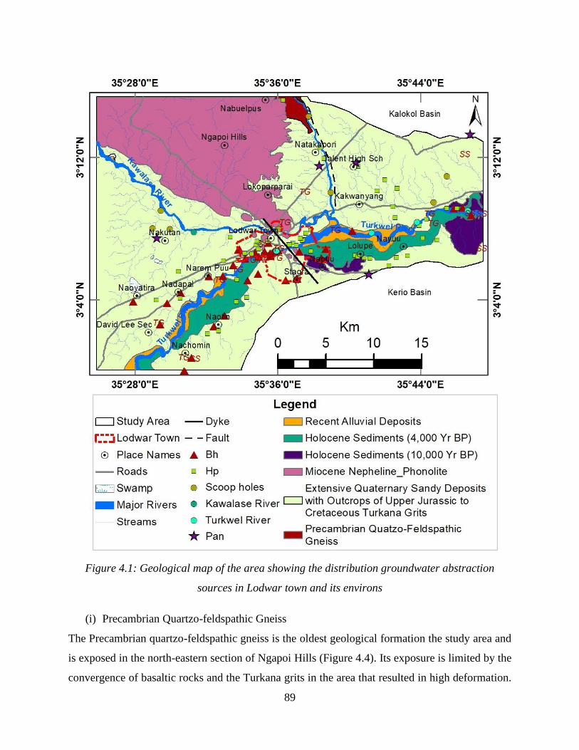
89

Figure 4.1: Geological map of the area showing the distribution groundwater abstraction

sources in Lodwar town and its environs

(i) Precambrian Quartzo-feldspathic Gneiss

The Precambrian quartzo-feldspathic gneiss is the oldest geological formation the study area and

is exposed in the north-eastern section of Ngapoi Hills (Figure 4.4). Its exposure is limited by the

convergence of basaltic rocks and the Turkana grits in the area that resulted in high deformation.

90

The immense folding and faulting of the quarzto-feldspathic gneiss made it challenging to measure

its dip angles accurately and strike directions. However, the general dip direction of this formation

was determined to be NW-SE. The quartzo-feldspathic gneisses were highly fractured, resulting

in fragmentation, transportation and deposition of quartzite boulders and feldspars minerals in the

Monti lagga to the Katapakori areas. The exposed thickness on this formation along the Monti

lagga is 3 m. Intrusions in these rocks were observed and caused the deformation and mineral

alterations.

(ii) Upper Jurassic to Cretaceous Turkana grits

The Turkana grits are mainly coarse-grained, sandstone-derived basement deposited on a dissected

basement topography by aggrading river systems. The outcrops of this formation were observed

at a few locations within the extensive Quaternary sands cover. The 'Turkana Grits' are covered by

Palaeogene volcanic rocks (35 Ma), which are thought to be the earliest evidence of plume-related

volcanism inside the East African Rift System (Agyemang et al., 2019). The grits encountered had

current and fluting features indicating their deposition in a deltaic environment with flood

washings (Rhemtulla, 1970). Around Nawaitorong areas, the Turkana grit is cemented by calcite

(Figure 4.2a). North-east of the municipality of Lodwar, on the eastern slope of the Ngapoi Hills,

the exposed grits consist of light grey-brown sandy clay covered by pebbly grit (Figure 4.2b) while

at Lorengelup areas, the Turkana grits overlie the Basement System. The Turkana grits at Naotin

is intercalated with a sandstone unit (Figure 4.2c) with graded bedding features (Figure 4.2d).

Extensive Quaternary sands derived from the Basement System rocks and wind-blown sands cover

the Turkana grits (Olago, 2018). The observed current features suggest localized sediment input

by alluvial fans (Agyemang et al., 2019). In most parts of the study area, this formation was

covered by the Quaternary sands and ranged from 0.3 to 1.0 meters where it was exposed.

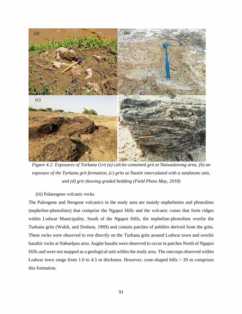
91

Figure 4.2: Exposures of Turkana Grit (a) calcite-cemented grit at Naiwaitorong area, (b) an

exposure of the Turkana grit formation, (c) grits at Naotin intercalated with a sandstone unit,

and (d) grit showing graded bedding (Field Photo May, 2018)

(iii) Palaeogene volcanic rocks

The Paleogene and Neogene volcanics in the study area are mainly nephelinites and phonolites

(nepheline-phonolites) that comprise the Ngapoi Hills and the volcanic cones that form ridges

within Lodwar Municipality. South of the Ngapoi Hills, the nepheline-phonolites overlie the

Turkana grits (Walsh, and Dodson, 1969) and contain patches of pebbles derived from the grits.

These rocks were observed to rest directly on the Turkana grits around Lodwar town and overlie

basaltic rocks at Nabuelpus area. Augite basalts were observed to occur in patches North of Ngapoi

Hills and were not mapped as a geological unit within the study area. The outcrops observed within

Lodwar town range from 1.0 to 4.5 m thickness. However, cone-shaped hills > 20 m comprises

this formation.

(a) (b)

(c) (d)

92

(iv) Holocene sediments

The Holocene sediments cover the southern bank of the Turkwel River with thicknesses ranging

from 2 to 7.5 m (Figure 4.3a, b), and they extended into the Napuu and Nayuu areas which are

between 5 and 8 km away from the river. The intermittent exposures of the Holocene sediments

and Turkana grits suggest that they have been deposited on former synclines. Besides, the

existence of folding features in the area is likely evidenced by widening and thinning of the

Turkwel River, where the soft Holocene sediments are exposed in the broad sections while the

hard Turkana grits occur in the constricted sections of the river banks. These sediments bear

erosional features as observed at Nayuu areas (Figure 4.3c, d), and form undulating landforms.

Particle sizes ranged from fine sand to medium gravel, and graded bedding was commonly

observed.

Figure 4.3: Exposed Holocene sediments illustrating thick deposits and erosional features at

Napuu-Nayuu areas, Turkana county

(a) (b)

(c) (d)

93

(v) Alluvial deposits

The alluvial deposits are considered the youngest geological formation in the study area and are

of recent age. They comprise fine sands, silts, clay, and gravels broken down from weathered

volcanic rocks and wind-blown sands. The thickness of the alluvial deposits within the Turkwel

and Kawalase rivers and Monti lagga ranged from 0.3 m to 1.5 m. In particular, the alluvial

deposits in the Turkwel River are extensive, especially to the east of the municipality of Lodwar.

A thin layer of alluvial deposits (<1 m thick) is found within the Kawalase River. However, these

deposits were found to be thicker at the confluence of the Kawalase River and the Monti lagga.

(b) Geological structures

Volcanic dykes and erosional surfaces were the major geological structures and features identified

in the study area. According to Hughes (1933), the Turkana grits are punctuated by dykes from

volcanic activity between Lodwar and Lokitaung areas. In the study area, a dolerite dyke dissecting

Lodwar town with a 45º NW trend was mapped for the first time. The dyke is exposed within the

Turkana grits at Kawalase lagga next to the drift road crossing. A dyke with similar orientation

and mineralogical composition was encountered in the northern part of the area near the Nabuelpus

area. These dolerite dykes appear to follow the NW-SE trending plane of weakness and have been

eroded more than the host Turkana Grits, forming linear trenches as observed by Rhemtulla (1970).

At Nabulon area next to the Turkwel River, a contact zone between the nepheline-phonolites and

the Turkana grits, with a 35 NE trend, was identified. A thin layer of conglomerate rock capped

the Turkana grit.

4.2.1.2 Remote sensing - Digital Terrain Model

(a) Satellite Imagery - STRM-based digital terrain model

The STRM of the study area indicated that the altitude ranges from 440 to 920 m above sea level.

High elevations are around the Ngapoi Hills ranging from 560 to 920 m asl. The Turkwel River

basin in the study area lies at altitudes < 520 m asl while the Kawalase occurs at altitudes ranging

between 470 to 530 m asl (Figure 4.4).

94

Figure 4.4: STRM of the study area within the Turkwel River watershed

(b) Stream lineament analysis

The STRM of the study area was used to delineate the watershed and to automatically generate the

stream network in the study area using a cell threshold of 700. The pre-digitized layers of the

Turkwel and Kawalase rivers were uploaded onto the watershed map to extract the river pour-

points and intersections (Figure 4.5). The results showed that the Kawalase River has multiple

streams flowing between 470 and 530 m asl on a fairly flat surface. It has also been found that all

the streams that contribute to the Monti lagga are situated in the western part of this river, forming

parallel drainage systems. The streams occur between linear series of escarpments that form

parallel, elongate landforms due to resistant Miocene volcanics outcropping east of Ngapoi Hills.

According to Boulton and Whittaker (2009) straight rivers fed by parallel streams flowing in the

same directions are typically located in a fault line. This phenomenon deduce that the Monti Lagga

is flowing on a fault. The streams which enter the Turkwel River directly within the study area

drain elevation areas ranging from 440 to 520 m asl. The remaining streams that drain the eastern

and northeastern parts occur at altitudes <500 m asl.

95

Figure 4.5: Drainage lineaments map of the area extracted from the STRM-based DEM

(c) Analysis of drone-acquired images

(i) Drone-based digital terrain model (DEM)

The analysis of drone acquired images provided a high-resolution digital terrain model of Lodwar

town showing elevations ranging from 460 to 598 m asl with the Lodwar Hill recording the highest

elevations (Figure 4.6). Generally, Kanamkemer area has high elevations between <460 and 560

m asl while the Nawaitorong, Napuu and some parts of California and Napetet areas recorded low

elevations of < 480 m asl. The DEM revealed the cone-like volcanic features in Lodwar town as

well as the outline of the Turkwel River. Lodwar airport's lack of drone images is a significant

limitation to the analysis using drone mapping.

96

Figure 4.6: Digital terrain model of Lodwar town produced from drone-acquired images that

excluding the airport section

(ii) Contour map

The contour map was used to depict elevations above sea level, revealing the shape of the

landforms in Lodwar town. The five-meter spacing contour map (Figure 4.7) revealed that the

floodplains are located at elevations < 465 m and comprise mainly the Turkwel River basin,

Nawaitorong, and Napuu areas, and consist primarily the alluvial deposits. Holocene sediments

cover the areas with elevations ranging from between 465 and 495 m asl while the Quaternary

wind-blown sandy deposits occur within 495 to 510 m asl. Turkana grits outcrops in areas occur

at elevations ranging between 515 to 520 m asl while the volcanic rocks occupy areas with

altitudes> 525 m asl.

97

Figure 4.7: Five-meter contour map of Lodwar town obtained from the drone-acquired images

(iii) Comparison of drone-based and STRM based DEM

Drone-based and STRM based DEM were analysed and compared within Lodwar town (Figure

4.8). The designated Survey of Kenya (SOK) datum point of Lodwar town located at 3° 07' N and

35° 36' E is 477 m and was used to determine the accuracy of the heights of the two digital elevation

models at the same point. The drone-based and STRM based slope angles were also compared

(Table 4.1).

Table 4.1: Comparison of STRM-based and drone-based digital elevation models and slope

angle maps

Remote sensing product

Drone-based DEM STRM-based DEM

(i) Digital terrain model

- Min and Max elevation (460 and 598 m asl)

- Elevation at datum point = 476 m - Close accuracy (-1m) from the SOK

datum

- Min and Max elevation (480 and 595 m asl)

- Elevation at datum point (492 m) - Wide gap (+12 m) from the SOK datum

point

(ii) Slope angle map

- Drone (0.00 to 72.20°) (average = 7.87°)

- Slope angles reveal deep sediment erosion and rock exposures along Turkwel and Kawalase rivers

- STRM: 0.00 to 33.02° (average = .2.87°) - Erosional features along Turkwel and

Kawalase Rivers not visible

98

Figure 4.8: Comparison between (a) drone-based DEM and (b) STRM-based DEM for Lodwar

town

Figure 4.9: Comparisons between (a) UAV drone-based slope angle map and (b) STRM-based

slope angle map

(iv) High-resolution orthomosaic

The orthomosaic obtained from the drone mapping has a vertical resolution of 0.5 m and is useful

in identifying ground features such as residential areas, rock outcrops, river and stream channels

as wells as demarcating geological boundaries. The grey areas were due to poor lighting conditions

from sandstorm occurrences at the time of mapping (Figure 4.10). Thus, it can also be used in

mapping/monitoring short-lived events.

99

Figure 4.10: Orthomosaic image obtained from the processing of the drone-acquired images.

The Mapping exercise did not cover Lodwar airport which is demarcated as a no-fly zone for

drones

Figure 4.11: Zooming inside the red rectangle within the orthomosaic image

100

(v) Textured 3D model

The texture 3D models acquired from processing drone-acquired images are used for urban

planning, population monitoring, and preparation of water supply networks and simulation. The

3D model is an interactive map that allows you to rotate in 360° for viewing and studying ground-

based objects (Figure 4.11).

Figure 4.12: Textured 3D model for Lodwar municipality excluding the airport area (original

model too large to be included in the report)

4.2.1.3 Rock sample collection and analysis

(i) Field description

The field specimens for quartzo-feldspathic gneiss, Turkana grits, Holocene sediments, sandstone,

conglomerate, grainstone, nepheline-phonolites, augite basalts, dolerites and alluvial deposits are

described in Appendixes 4-1 to 4-6.

a. Precambrian quartzo-feldspathic gneiss

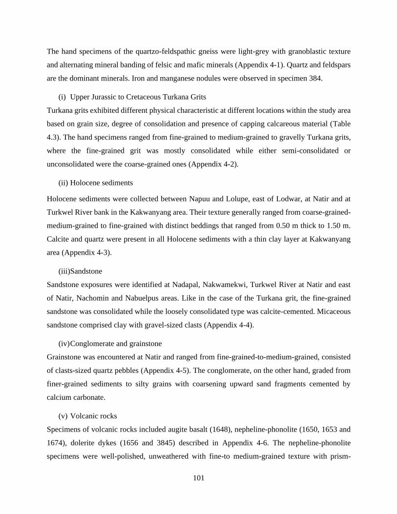
101

The hand specimens of the quartzo-feldspathic gneiss were light-grey with granoblastic texture

and alternating mineral banding of felsic and mafic minerals (Appendix 4-1). Quartz and feldspars

are the dominant minerals. Iron and manganese nodules were observed in specimen 384.

(i) Upper Jurassic to Cretaceous Turkana Grits

Turkana grits exhibited different physical characteristic at different locations within the study area

based on grain size, degree of consolidation and presence of capping calcareous material (Table

4.3). The hand specimens ranged from fine-grained to medium-grained to gravelly Turkana grits,

where the fine-grained grit was mostly consolidated while either semi-consolidated or

unconsolidated were the coarse-grained ones (Appendix 4-2).

(ii) Holocene sediments

Holocene sediments were collected between Napuu and Lolupe, east of Lodwar, at Natir and at

Turkwel River bank in the Kakwanyang area. Their texture generally ranged from coarse-grained-

medium-grained to fine-grained with distinct beddings that ranged from 0.50 m thick to 1.50 m.

Calcite and quartz were present in all Holocene sediments with a thin clay layer at Kakwanyang

area (Appendix 4-3).

(iii)Sandstone

Sandstone exposures were identified at Nadapal, Nakwamekwi, Turkwel River at Natir and east

of Natir, Nachomin and Nabuelpus areas. Like in the case of the Turkana grit, the fine-grained

sandstone was consolidated while the loosely consolidated type was calcite-cemented. Micaceous

sandstone comprised clay with gravel-sized clasts (Appendix 4-4).

(iv) Conglomerate and grainstone

Grainstone was encountered at Natir and ranged from fine-grained-to-medium-grained, consisted

of clasts-sized quartz pebbles (Appendix 4-5). The conglomerate, on the other hand, graded from

finer-grained sediments to silty grains with coarsening upward sand fragments cemented by

calcium carbonate.

(v) Volcanic rocks

Specimens of volcanic rocks included augite basalt (1648), nepheline-phonolite (1650, 1653 and

1674), dolerite dykes (1656 and 3845) described in Appendix 4-6. The nepheline-phonolite

specimens were well-polished, unweathered with fine-to medium-grained texture with prism-

102

shaped nepheline crystals, plagioclase feldspars, magnetite, and haematite. The dolerite dyke in

Turkana grits consisted of plagioclase and pyroxene minerals with inclusions of the grits indicating

the Turkana grits are older (Appendix 4-6).

a) Alluvial deposits

Alluvial deposits consisted of white to brown sandy deposits with dark-coloured organic matter

and graded bedding structures. There was no reaction of HCl with feldspars, biotite and mica grains

were observed. The deposits mainly consisted of sands, silts, clay and gravel.

b) Petrographic analysis

The rock samples were assigned specific codes ranging from 1650 to 3858 for analysis. These

codes are indicated below in brackets. The rock samples petrographically analysed included;

nepheline-phonolite (1650), dolerite dykes (1656 and 3845), conglomerate (3857), sandstone

(1659, 3833 and 3858), Turkana grits (1656 and 3831) and the quartzo-feldspathic gneiss (3843

and 3844).

(i) Nepheline-phonolite

The nepheline-phonolite (sample number 1650) had anhedral prismatic nepheline crystals (Figure

4.13). The crystals are anhedral, assuming the hexagonal crystal symmetry and altered in parts to

sodalite and turbid anorthoclase feldspar. The fine-grained groundmass of green aegirine-augite,

anorthoclase, and nepheline contains euhedral haematite grains. Cataclastic deformation (a later,

lower-temperature phase of strain localisation in plutonic rocks) of plagioclase was observed under

PPL and XPL, forming deformation bands that correlated with the shear strain. The hematite grains

appeared to be larger in the deformation zone. In a thin fragment, rare nepheline microphenocrysts,

partially modified to sodalite, and turbid anorthoclase feldspar are also present in the fine-grained

groundmass.

103

Figure 4.13: Microphotograph of the nepheline-phonolite (sample 1650) observed under (a)

PPL and (b) XPL showing the prismatic nepheline crystals and euhedral hematite grains, with

cataclastic deformation of plagioclase was observed in the thin section

(ii) Dolerite

Dolerite is a dark-grey to black intrusive rock with fine to medium-grained groundmass and was

identified occurring as a dyke in the Turkana grits. Instead of a thin section preparation, a thick

section (> 30µ) was achieved in the slice preparation and has been used for fluid or melt inclusion

and melt inclusion analysis (Grundmann and Scholz, 2015). However, Figure 4.14 shows

fracturing in PPL and with no fluid inclusion entrapment observed. Possible twinning of minerals

can be observed in XPL (Figure 4.14b), however, a confirmation in thin section (< 30µ is required).

In thin sections, most dolerites show numerous colourless grains of quartz and feldspars, where

the feldspars assumed prismatic habit (Shekhar et al., 2018). Primary minerals identified include

plagioclase, pyroxene, and amphiboles, where the plagioclase crystals are acicular, and the

pyroxene grains are subhedral with chloritised outlines while the secondary minerals included

chlorite and quartz (Mugerwa, 2015).

104

Figure 4.14: Microphotograph of the dolerite dyke rock within the Turkana grits shows

fracturing in PPL and with no fluid inclusion entrapment observed, in XPL, possible twinning of

is observed. However, this can be further evaluated in a slice < 30 µ

(iii) Conglomerate

Specimen 3857 of conglomerate capping the Turkana grit at its contact zone with the nepheline

phonolite revealed angular quartz and feldspar fragments cemented by clay and some calcite.

Colourless sub-rounded quartz minerals are observed in both in XPL (a) and PPL (b), and prismatic

nepheline crystals were present in the rock sample (Figure 4.15). With angular altered volcanic

rock fragments, there is poorly defined sedimentary banding. There are also altered biotite grains,

which indicate alkalic or acidic volcanism. The conglomerate is cemented with coarse-grained

sparry calcite cement which fills the clasts in cracks as well. The feldspars present are andesite and

deep brown sodic amphibole like that described by Muia (2015) and Walsh and Dodson (1969).

(a) (b)

Possible twinning

105

Figure 4.15: Microphotograph of the conglomerate sample (3857) under (a) PPL and (b) XPL

showing sub-rounded quartz grains and prismatic nepheline crystal with distinct cleavages

(iv) Sandstone

Three sandstone samples (1659, 3833, and 3858) have medium-sized grains (Figure 4.16 a and b)

comprised of quartz, feldspars, and biotite. The fined grained compact sandstone sample (Figure

4.19 c and d) show dominant feldspar grains under XPL (d). What appears to be fluid inclusion

features had diameters ranging from less than 20.00 µm to 130.47 µm is observed in in Figure 4.6

c and d. indicating that temperatures >100 °C were not reached during the burial history of the

sandstone. The same my represent bubbles trapped inn the slice during the thin-section preparation.

The sandstone was highly fractured with some of the microfractures filled with brown minerals,

possibly iron and oxyhydroxides. The poorly sorted sand and gravels in the coarse-grained

sandstone and existence of fractures in the fine-grained counterpart suggest high permeability of

sandstone in the study area. The coarse-grained sandstone (Figure 4.16 e and f) comprised mainly

of sub-rounded to well-rounded quartz pebbles cemented by calcite and carbonate.

Cryptocrystalline chert, micro micaceous mudstone, siltstone and stretched quartz grains dominate

the mineral framework. Fewer feldspars grains were present in the coarse-grained sandstone as

compared to those present in the fine-grained specimens.

(a) (b)

Cleavage Cleavage

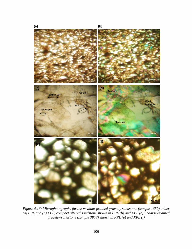
106

Figure 4.16: Microphotographs for the medium-grained gravelly sandstone (sample 1659) under

(a) PPL and (b) XPL, compact altered sandstone shown in PPL (b) and XPL (c); coarse-grained

gravelly-sandstone (sample 3858) shown in PPL (e) and XPL (f)

(a) (b)

(c) (d)

(e)(f)

130.47 µm

98.42 µm

<20 µm

<74.64 µm

Fracture

Fracture

Filled fractures

107

(v) Turkana grits

The Turkana grit samples (1656 and 3831) predominantly consists of fine to coarse arkosic

sandstone suggesting fluvial deposition and comprised mainly quartz and feldspars (25-40%),

cemented by calcite. The yellow crystals observed under PPL were regarded as staurolite,

and green are hornblende minerals. The Turkana grit in contact with the dolerite dyke (Figure 4.17

a and b) had zoning features and altered minerals caused by contact metasomatism. The quartz

and feldspars are anhedral-shaped and are poorly sorted within the calcite matrix with grains

ranging from 0.25 to 1.00 mm (Figure 4.17 c and d).

Figure 4.17: Microphotographs of the Turkana grit samples showing zoning features (a and b)

calcite-cemented matrix on quartz and feldspars minerals (b and c)

108

(vi) Quartzo-feldspathic gneiss

Two samples of the quartzo-feldspathic gneiss collected at the same location indicate different

mineralogical characteristics. Sample 3343 (Figure 4.18 a and b) was attached to the igneous

intrusion and showed highly deformed minerals caused by high-grade metamorphism. Quartz and

feldspars are the dominant minerals observed in sample 3344 (Figure 4.18 c and d), and biotite

comprises 5% of the mineralogy occurring as an accessory mineral. The feldspars present include

altered orthoclase, microcline, and plagioclase. The majority of the orthoclase grains have been

converted to small flakes of sericite while the initial biotite grain has reacted to oxides,

orthopyroxene, and (inferred) melt during contact metamorphism. The partly replaced biotite

grains are surrounded by relict plagioclase in sieve texture with spaces filled with quartz and

feldspars.

Figure 4.18: Microphotographs of the quartzo-feldspathic gneiss adjacent to the dolerite

intrusion showing highly deformed surfaces (a and b) and fine-grained surface of quartz and

feldspars further away from the intrusion (c and d)

(a)

(c) (d)

(b)

109

4.2.1.4 Geochemistry of rock samples

The geochemistry of the rock samples has been described based on the results of the major

elements and the concentration of trace metals and trace elements using XRF. The major elements

were expressed as oxides of SiO2, Al2O3, CaO, MgO, Na2O, K2O, TiO2, MnO, Fe2O, and LOI

(Appendix 4-7 and Appendix 4-8). The sum of the concentration of each oxide ranged from 97.80

to 99.99 %. The trace elements comprised Cr, Co, Ni, Cu, Zn, As, Se, Mo, and Pb and are

expressed as a percentage (Appendix 4-9).

(i) Metamorphic rocks

In the three rock samples (3841, 3843 and 3846) of the quartzo-feldspathic gneiss, silica (SIO2)

ranged between 52.83 to 53.71 wt % and was the most abundant oxide. The abundance of Al2O3

(18.20 to 19.95 wt %) indicates the presence of aluminosilicates and clay minerals such as kaolinite

as a result of weathering processes. As in the case of most metamorphic gneisses, all the specimens

of the quartzo-feldspathic gneiss had high K2O content with K2O/Na2O ratios exceeding 1 (1.62,

1.19, 1.10), indicating high-temperature recrystallization. The rock samples are poor in

ferromagnesian elements - MnO (0.25 wt %), TiO2 (0.19 wt %) and MgO (0.09 wt%). Their An-

Ab-Or normative classification plot in the granite field (Figure 4.19 a), as a result of low CaO

content (2.15 wt %) (Irvine and Baragar, 1971). AFM classification of the rock samples (Figure

4.22) indicate they are calc-alkaline (Figure 4.19 b).

The major elements present include Ca (8.60 %), Fe (3.90%), Mg (2.42%), Al (2.30%), K (0.22%),

Mn (0.15%) and P and S (0.04%) each. The lack of Na in all the rocks samples suggests that the

quartzo-feldspathic gneiss is rich in anorthite, a characteristic of the granulite facies of

metamorphic rocks. In terms of trace elements, Co, As, Se, Mo and Pb were not detected in all

the rock samples. Zn was 0.01% in all the samples as well as that of Ti in sample 3841 and 3843.

Cr was 0.01% in sample 3841 and 0.08% in sample 3843 and 3846 suggesting they are more

enriched in pyroxenes and mica than sample 3841. Cu was only present in sample 3841 (0.03%)

(Table 4.2).

110

Table 4.2: Results for the major oxides, major elements and trace metals in the quartzo-

feldspathic gneiss (three rock samples, see Appendix 4-7 to 4-9 for detailed results per sample)

Major element oxides

Rock sample SIO2 Al2O3 CaO MgO Na2O K2O TiO2 MnO Fe2O3 LOI

3841-18 53.71 18.2 1.52 1.07 4.03 6.52 0.19 0.27 3.92 9.63

3843-18 52.83 19.95 2.15 0.01 4.93 5.87 0.18 0.25 4.31 8.66

3846-18 53.21 19.89 2.49 0.09 5.01 5.5 0.23 0.24 4.49 8.84

Average 53.25 19.35 2.05 0.39 4.66 5.96 0.20 0.25 4.24 9.04

Major elements

Na Mg Al P S K Ca Mn Fe

3841-18 nd 1.96 1.71 0.03 0.07 0.37 12.63 0.07 1.12

3843-18 nd 2.89 1.82 0.05 nd 0.17 5.34 0.18 4.26

3846-18 nd 2.42 3.38 0.03 0.01 0.14 7.82 0.20 6.32

Average 2.42 2.30 0.04 0.04 0.22 8.60 0.15 3.90

Trace elements

Ti Cr Co Ni Cu Zn As Se Mo Pb

3841-18 0.01 0.01 nd 0.00 0.03 0.01 nd nd nd nd

3843-18 0.01 0.08 0.00 0.02 nd 0.01 nd nd nd nd

3846-18 nd 0.08 0.00 0.01 nd 0.01 nd 0.00 nd nd

Average 0.01 0.06 0.00 0.01 0.03 0.01 nd 0.00 nd nd

Figure 4.19: (a) An-Ab-Or normative classification based on O’Connor (1965) and 9b) AFM

diagram for the quartzo-feldspathic gneiss showing high Na2O and K2O content (after Irvine and

Baragar, 1971)

111

(ii) Sedimentary rocks

(a) Turkana grits

A total of eighteen rock samples of the Turkana grits were analysed for major elements while 11

of these samples were analysed for major and trace elements. The results of the major elements

represented complex geochemistry among the different rock specimens (Figure 4.20). Generally,

the chemical and mineralogical compositions of the sediments and sedimentary rocks are

extremely diverse due to the varied origin of sediments and resulting end-members. Application

of the K means clustering algorithm revealed four unique clusters of the Turkana grits in the study

area (Table 4.3). Table 4.4 shows the class centroids for each cluster based on the compositions of

the major elements in the rock samples, while Table 4.5 present the description of their chemical

compositions.

Table 4.3: Description of the different clusters of the Turkana grits based K Means Clustering

Algorithm

Turkana grit Clusters Description

Cluster 1: Fine-grained

Turkana grits

Cluster 1 had seven members (1646, 1649,1651, 1654, 1655, 3835 and, 3839) and

represented specimens of the Turkana grits collected within Lodwar town and at

Nakutan area.

Cluster 2: Gravelly

Turkana grits

Two rock samples comprised Cluster 2 (1652 and 3848) and were collected north-

east of Lodwar town at Kakwanyang and to the east of Talent High school.

Cluster 3: Semi-

consolidated sandy

Turkana grits

Cluster 3 comprised six rock samples of the Turkana grits (1671, 1672, 1673, 3831,

3836, and 3838) that occurred adjacent to the Holocene sediments. The rock

specimens were mainly sandy and semi-consolidated and often capped by a highly

consolidated gravelly layer.

Cluster 4: Consolidated

Turkana grits

Cluster 4 comprised three rock samples of the Turkana grits (3830, 3849 and 3856)

recorded at Nachomin, Nakadukui and Natirnalulung areas. Like Cluster 2

samples, these members were observed at isolated locations and often capped by

calcareous material.

112

Table 4.4: Class centroids for each cluster based on the compositions of the major elements in

the rock samples

Class SIO2 Al2O3 CaO MgO Na2O K2O TiO2 MnO Fe2O3 LOI

1 53.86 8.53 13.58 4.82 0.77 2.06 0.59 0.45 2.83 11.76

2 51.03 4.12 33.57 3.54 0.39 0.63 0.21 0.14 1.49 4.35

3 65.60 11.00 5.03 1.57 0.14 1.92 0.53 0.17 3.43 10.24

4 28.81 3.94 28.03 5.07 0.27 0.76 0.20 0.35 2.06 29.88

Figure 4.20: Variations of the chemical compositions of the major elements among the clusters

of Turkana grits

113

Table 4.5: Description of the major oxides, major and trace elements of the four clusters of the

Turkana grits

Cluster Major Oxides Major elements Trace elements

Cluster 1:

Fine-grained

Turkana grits

- Characterised by high MgO,

Na2O, K2O and MnO.

- SiO2 ranged from 45.70 to

60.48 %, CaO (7.80 -18.24%),

- LOI (7.88-17.37%), Al2O3

(3.89 - 16.40%), MgO (0.02 -

9.21%), Fe2O3 (1.32 - 7.90%),

- K2O (0.98 - 4.03%), TiO2

(0.09 - 2.40%), and the least

composition was Na2O (0.02

- 1.98%).

- Ca, Al, and Fe are the

most abundant major

elements with median

values of 8.83%, 2.80 %

and Fe 2.42 %

respectively

- K, Mg, Mn, Na had

median concentrations

<0.50%.

- Ti, Cr, Co, Ni, Cu, Zn,

Se and Mo had

median values

<0.01% while As,

and Pb was not

within detectable

limits in this cluster

Cluster 2:

Gravelly

Turkana grits

- Characterised by very high

CaO (30.14 - 37.00%) and

low Fe2O3 (1.17 -1.81%)

- SiO2 (48.36 – 53.70%), Al2O3

(4.03-4.21%) was also

relatively lower than that of

Clusters 1 and 3

- Like in cluster 1, Ca

(9.08%), Al (2.62%),

and Fe (2.22%) were

the most abundant

major elements

- Mg was 0.74% P, S, and

K were < 0.05% while

Na was not detected in

specimens of this

cluster.

- Cu, As, and Pb were

below detectable

limits while Ti was

0.07%.

- Cr, Ni, Co, Zn, Se and

Mo was <0.01%

Cluster 3:

Semi-

consolidated

sandy

Turkana grits

- Highest compositions of SiO2

(60.80 – 71.06 %), Al2O3

(4.81-15.87%), K2O (0.94 –

2.51%), TiO (0.32 – 0.89%),

Fe2O3 (2.49 – 4.90%), CaO

(2.76 – 9.80), with the

lowest levels of MgO (0.03 –

3.02 %), and Na2O (0.09 –

0.21%) than in Clusters 1, 2

and 4.

- Ca (9.08%), Al (2.62%),

and Fe (2.22%) were

most abundant than

the rest of the trace

elements.

- Mg was 0.74%, while P,

S, and K were below

0.05%. Na was not

detected like cluster 2

- Ti was 0.05%

- As, Se and Pb were

below detectable

limits in this cluster.

- The rest of the

elements (Ti, Cr, Co,

Ni, Cu, Zn, and Mo

were <0.01%

Cluster 4:

Consolidated

Turkana grits

- High concentration of CaO

(15.80 – 38.15 %) after

cluster 2 and

- Highest moisture and

volatile materials (25.87 -

34.27%) and MgO (0.05 –

9.15%), and the least SiO2

(<40.09%) content among all

the four clusters.

- Major elements

showed the highest Ca

concentration of the

four clusters (17.08%)

- Al was 1.78%, Fe

1.53% and Mg 0.70%,

- K, P and S were below

0.05%

- Concentration of all

trace elements was

<0.02%

114

Table 4.6: Descriptive statistics for the major elements (Cluster 1 to 4)for the different groups of

Turkana grits samples (SD – standard deviation)

(a) Cluster 1: Descriptive statistics for the Cluster 1 Turkana grits samples (wt. %)

Statistic SiO2 Al2O3 CaO MgO Na2O K2O TiO2 MnO Fe2O3 LOI

Minimum 45.70 3.89 7.80 0.02 0.02 0.98 0.14 0.09 1.32 7.88

Maximum 60.48 16.40 18.24 9.21 1.98 4.03 2.40 2.01 7.90 17.37

Range 14.78 12.51 10.44 9.19 1.96 3.05 2.26 1.92 6.58 9.49

Median 56.92 9.12 14.01 6.10 0.87 1.51 0.17 0.19 1.95 9.89

Mean 53.86 8.53 13.58 4.82 0.77 2.06 0.59 0.45 2.83 11.76

Variance 43.48 19.51 12.38 14.78 0.58 1.21 0.69 0.48 5.53 15.44

SD 6.59 4.42 3.52 3.84 0.76 1.10 0.83 0.69 2.35 3.93

(b) Cluster 2: Descriptive statistics for the gravelly Turkana grits (wt. %)

Statistic SiO2 Al2O3 CaO MgO Na2O K2O TiO2 MnO Fe2O3 LOI

Minimum 48.36 4.03 30.14 1.06 0.20 0.61 0.19 0.13 1.17 1.88

Maximum 53.70 4.21 37.00 6.01 0.58 0.65 0.23 0.15 1.81 6.81

Range 5.34 0.18 6.86 4.95 0.38 0.04 0.04 0.02 0.64 4.93

Median 51.03 4.12 33.57 3.54 0.39 0.63 0.21 0.14 1.49 4.35

Mean 51.03 4.12 33.57 3.54 0.39 0.63 0.21 0.14 1.49 4.35

Variance 14.26 0.02 23.53 12.25 0.07 0.00 0.00 0.00 0.20 12.15

SD 3.78 0.13 4.85 3.50 0.27 0.03 0.03 0.01 0.45 3.49

(c) Cluster 3: Descriptive statistics for the Semi-consolidated sandy Turkana grits (wt. %)

Statistic SiO2 Al2O3 CaO MgO Na2O K2O TiO2 MnO Fe2O3 LOI

Minimum 60.80 4.81 2.76 0.03 0.09 0.94 0.32 0.08 2.40 5.47

Maximum 71.06 15.87 9.80 3.02 0.21 2.51 0.89 0.32 4.90 24.91

Range 10.26 11.06 7.04 2.99 0.12 1.57 0.57 0.24 2.50 19.44

Median 64.05 11.29 3.73 1.92 0.13 2.06 0.46 0.11 3.31 7.77

Mean 65.60 11.00 5.03 1.57 0.14 1.92 0.53 0.17 3.43 10.24

Variance 19.29 12.78 8.11 1.59 0.00 0.28 0.04 0.01 0.81 53.83

SD 4.39 3.57 2.85 1.26 0.04 0.53 0.21 0.12 0.90 7.34

(d) Cluster 4: Descriptive statistics for the consolidated Turkana grits (wt. %)

Statistic SiO2 Al2O3 CaO MgO Na2O K2O TiO2 MnO Fe2O3 LOI

Minimum 21.83 3.41 15.80 0.05 0.03 0.54 0.18 0.15 1.65 25.87

Maximum 40.09 4.21 38.15 9.15 0.57 1.12 0.23 0.71 2.73 34.27

Range 18.26 0.80 22.35 9.10 0.54 0.58 0.05 0.56 1.08 8.40

Median 24.51 4.20 30.14 6.01 0.20 0.61 0.19 0.19 1.81 29.49

Mean 28.81 3.94 28.03 5.07 0.27 0.76 0.20 0.35 2.06 29.88

Variance 97.22 0.21 128.22 21.37 0.08 0.10 0.00 0.10 0.34 17.75

SD 9.86 0.46 11.32 4.62 0.28 0.32 0.03 0.31 0.58 4.21

115

(b) Holocene sediments

The geochemistry of the Holocene sediments is based on specimens collected along with selected

profiles in the east of Lodwar town, between Napuu and Lolupe, Turkwel River at Kakwanyang

and Natirnalulung area.

East of Lodwar town

Holocene sediments east of Lodwar town showed relatively high silica content (57.97 - 69.67 wt

%) with the top layer (3824) having low SiO2 than the bottom bed (3825) based on median values.

The top layer was also richer in Al2O3 (16.52 %), Fe2O3 (7.97 wt %) and LOI (11.26 wt %) against

that of the bottom layer; Al2O3 (11.89 wt %), Fe2O3 (3.14 wt %), and 4.10% LOI content. Like in

all the samples of the Holocene sediments in the study area, Na was not present in the sediment

samples (3824 and 3825). Al (4.17 wt %), Fe (4.03 wt %), Ca (3.21 wt %), and Mg (1.01 wt %)

were the most abundant major elements, indicating metamorphic origin. In terms of trace elements,

Ti, Cr, Cu and Zn occurred in the two specimens of the Holocene sediments east of Lodwar town

with higher concentrations observed in the upper layer (3824) than in sample 3825 (Table 4.7).

Co, Ni and Mo had concentrations < 0.00 wt % while As, Se and Pb were not detected.

Table 4.7: Results and summary statistics for the major oxides, major and trace elements of the

Holocene sediments East of Lodwar town

Major element oxides (wt %)

Description SIO2 Al2O3 CaO MgO Na2O K2O TiO2 MnO Fe2O3 LOI

3824-(A) 57.97 16.52 2.06 1.37 0.14 1.39 0.94 0.12 7.97 11.26

3825-(B) 69.97 11.89 5.34 1.97 0.09 2.02 0.43 0.08 3.14 4.10

Average 63.97 14.21 3.70 1.67 0.12 1.71 0.69 0.10 5.56 7.68

Major elements (wt %)

Description Na Mg Al P S K Ca Mn Fe

3824-(A) nd 1.18 5.32 0.04 0.18 0.69 1.49 0.09 5.67

3825-(B) nd 0.84 3.01 0.05 0.00 0.26 4.93 0.07 2.40

Average nd 1.01 4.17 0.05 0.09 0.47 3.21 0.08 4.03

Trace elements (wt %)

Description Ti Cr Co Ni Cu Zn As Se Mo Pb

3824-(A) 0.13 0.01 0.00 0.00 0.01 0.02 nd nd 0.00 nd

3825-(B) 0.05 0.01 0.00 0.00 nd 0.01 nd nd 0.00 nd

Average 0.09 0.01 0.00 0.00 0.01 0.02 nd nd 0.00 nd

116

Napuu/ Lolupe area

Holocene sediments between Napuu and Lolupe areas exhibited four distinct layers; layer A, a

compact light-coloured fine-grained sediment (3820), layer B, dark-coloured sediment (3821),

layer C, slightly light-coloured bed (3822) and a bottom layer (D) consisting of a fine-grained

sandy layer (3823). SiO2 was observed to decrease from layer A to C (66.90 to 51.80 wt %) and a

significant increase to 80.85 wt % in layer D. There was an alternating decrease and increase in

Al2O3 content from top to bottom (Table 4.9) a characteristic observed in the compositions of CaO

and K2O. Layer B (7.70%) and C (7.71%) had relatively similar Fe2O3 content that was higher

than in layer A (3.78%) and D (1.11%). Of all the four layers (A, B, C and D), only the bottom

layer D (3823) had Na, with a concentration of 0.11 wt %. Like in the case of Holocene sediments

East of Lodwar, Al (4.23 wt %), Fe (3.91 wt %), Ca (2.19 wt %), and Mg (0.47 wt %) are the most

abundant major elements, though with slightly lower Fe, Ca and Mg content than at east of Lodwar.

The occurrence of trace elements was like at East of Lodwar town (Ti, Cr, Cu and Zn) with

increasing concentrations of Ti from the bottom (3823) to the top (3920) layer (Table 4.8).

117

Table 4.8: Results and summary statistics for the major oxides, major and trace elements of the

Holocene sediments at Napuu/Lolupe area

Major element oxides (wt %)

Lab No. SiO2 Al2O3 CaO MgO Na2O K2O TiO2 MnO Fe2O3 LOI

3820 (A) 66.90 16.05 2.74 1.50 0.15 2.43 0.76 0.10 3.78 5.50

3821 (B) 55.10 14.70 2.55 1.47 0.10 1.87 1.34 0.19 7.70 14.16

3822 (C) 51.80 16.42 2.62 0.11 0.17 1.84 1.24 0.20 7.71 17.09

3823 (D) 80.85 10.92 2.61 0.12 0.12 1.68 0.14 0.17 1.11 2.07

Minimum 51.80 10.92 2.55 0.11 0.10 1.68 0.14 0.10 1.11 2.07

Maximum 80.85 16.42 2.74 1.50 0.17 2.43 1.34 0.20 7.71 17.09

Median 61.00 15.38 2.62 0.80 0.14 1.86 1.00 0.18 5.74 9.83

SD 13.16 2.51 0.08 0.79 0.03 0.33 0.55 0.05 3.23 7.08

Major elements (wt %)

Na Mg Al P S K Ca Mn Fe

3820 (A) nd 0.64 3.76 0.07 0.01 0.39 2.51 0.09 3.03

3821 (B) nd 0.73 4.87 0.07 0.00 0.64 1.88 0.14 5.16

3822 (C) nd 0.69 4.69 0.06 nd 0.62 1.88 0.14 4.80

3823 (D) 0.11 0.09 1.72 0.03 0.01 0.11 2.50 0.03 1.23

Minimum 0.11 0.09 1.72 0.03 0.00 0.11 1.88 0.03 1.23

Maximum 0.11 0.73 4.87 0.07 0.01 0.64 2.51 0.14 5.16

Median n/a 0.67 4.23 0.07 0.01 0.50 2.19 0.12 3.91

SD n/a 0.30 1.44 0.02 0.00 0.25 0.36 0.05 1.80

Trace elements (wt %)

Ti Cr Co Ni Cu Zn As Se Mo Pb

3820 (A) 0.14 0.01 0.00 0.00 0.00 0.01 nd nd 0.00 nd

3821 (B) 0.19 0.01 0.00 0.00 0.00 0.02 nd nd 0.00 nd

3822 (C) 0.19 0.01 0.00 0.00 0.00 0.02 nd nd 0.00 nd

3823 (D) 0.02 0.01 nd 0.00 0.00 0.01 nd nd 0.00 nd

Holocene sediments at Turkwel River bank near Kakwanyang area

The thick layer of Holocene sediments found at the Turkwel River near Kakwanyang consisted of

four distinct layers A, B, C and D represented by sample codes 3852 to 3855. SiO2 (46.07-48.79

%) was comparatively lower than the Holocene sediment in Lodwar and between Napuu and

Lolupe areas. Al2O3 decreased from the top (18.80 %) to the bottom (9.87 %) of the deposit, while

CaO showed the reverse (Figure 4.26). Fe2O3 were comparatively higher than in Lolupe and Napuu

and decreased from Layer B (15.97 %) to the bottom layer (D) (3.90 %). Similar characteristic was

observed for the occurrence of K2O and Na2O and minor elements (Ca, Al and Fe) (Table 4.9). Na

was detectable in the Holocene sediments at Turkwel River bank near Kakwanyang up to 0.19 wt

%. Although Al, Fe, Mg, and Ca are the most abundant major elements like at East of Lodwar,

118

Napuu and Lolupe areas, Ca concentrations were relatively higher (11.34 %) suggesting increased

carbonate content and low composition of clay minerals. The occurrence of trace elements was

<0.02 wt % in all the samples (3852 to 3855).

Table 4.9: Results and summary statistics for the major oxides, major and trace elements of the

Holocene sediments at Turkwel River bank near Kakwanyang area

Major oxides (wt %)

Description SiO2 Al2O3 CaO MgO Na2O K2O TiO2 MnO Fe2O3 LOI

3852 (A) 48.79 18.90 1.25 1.93 1.30 3.24 1.20 0.14 9.53 13.16

3853 (B) 43.69 18.70 1.01 0.08 1.96 3.41 1.41 0.17 13.15 15.97

3854 (C) 46.51 13.95 8.15 3.05 0.99 2.41 0.14 0.15 6.51 16.72

3855 (D) 46.07 9.87 19.50 2.87 0.87 1.57 0.75 0.60 3.90 12.91

Minimum 43.69 9.87 1.01 0.08 0.87 1.57 0.14 0.14 3.90 12.91

Maximum 48.79 18.90 19.50 3.05 1.96 3.41 1.41 0.60 13.15 16.72

Median 46.29 16.33 4.70 2.40 1.15 2.83 0.98 0.16 8.02 14.57

SD 2.09 4.31 8.67 1.36 0.49 0.85 0.56 0.22 3.98 1.94

Major elements (wt %)

Description Na Mg Al P S K Ca Mn Fe

3852 (A) 0.00 1.80 4.23 0.06 0.06 0.36 5.22 0.12 3.96

3853 (B) nd 0.75 1.79 0.09 0.07 0.26 14.79 0.71 2.29

3854 (C) 0.00 4.53 2.06 0.03 0.08 0.12 13.32 0.13 1.17

3855 (D) 0.19 0.37 1.31 0.08 0.02 0.40 9.36 0.26 1.84

Minimum 0.00 0.37 1.31 0.03 0.02 0.12 5.22 0.12 1.17

Maximum 0.19 4.53 4.23 0.09 0.08 0.40 14.79 0.71 3.96

Median 0.00 1.28 1.93 0.07 0.06 0.31 11.34 0.19 2.06

SD 0.11 1.88 1.29 0.03 0.02 0.13 4.30 0.28 1.19

Trace elements (wt %)

Description Ti Cr Co Ni Cu Zn As Se Mo Pb

3852 (A) 0.10 0.01 0.00 0.00 0.02 0.02 nd nd 0.00 nd

3853 (B) 0.10 0.01 0.00 0.00 0.00 0.01 nd nd 0.00 nd

3854 (C) 0.01 0.01 nd 0.00 nd 0.01 nd nd 0.00 nd

3855 (D) 0.01 0.01 0.00 0.00 0.00 0.01 nd nd 0.00 nd

Holocene sediments at Natir

The three samples of Holocene sediments at Natir consisted of the upper layer A (3829), the middle

layer B (3827) and the lower layer C (3826). Significant variations in SiO2 content were observed,

with Layer A at 68.97 wt %, Layer B at 12.89 % and Layer C at 24.91 wt %. Different patterns

119

were found in the Al2O3 material, where the first layer had the most composition (10.21 %),

followed by the bottom layer (4.89wt %) and then middle layer B (2.01 wt %). Similar

characteristics have been observed for K2O, TiO2 and Fe2O3. Layer B was determined to have

elevated CaO, LOI and Ca levels relative to Layer A (3829) and C (3826) (Table 4.10). Al, Fe,

Mg, and Ca are the most abundant major elements but with the highest Ca compositions (18.98 %)

as compared to at Lodwar, Napuu, Lolupe and at Turkwel River near Kakwanyang. Al, Fe and Mg

contents are observed to generally decrease with increasing levels of Ca as you move eastwards

from Lodwar town. The occurrence of trace elements was generally low (< 0.02 wt %) except for

Layer A (3829) that had levels of 0.06 wt % of Ti.

Table 4.10: Results and summary statistics for the Major oxides, major and trace elements of the

Holocene sediments at Natir

Major element oxides (wt %)

Description SiO2 Al2O3 CaO MgO Na2O K2O TiO2 MnO Fe2O3 LOI

3829 (A) 68.97 10.21 1.82 2.67 0.05 1.81 0.62 0.09 4.73 8.48

3827 (B) 12.89 2.01 45.78 0.07 0.04 0.06 0.14 0.52 1.99 36.31

3826 (C) 24.91 4.89 27.15 7.01 0.08 0.72 0.27 0.30 2.14 32.00

Minimum 12.89 2.01 1.82 0.07 0.04 0.06 0.14 0.09 1.99 8.48

Maximum 68.97 10.21 45.78 7.01 0.08 1.81 0.62 0.52 4.73 36.31

Median 24.91 4.89 27.15 2.67 0.05 0.72 0.27 0.30 2.14 32.00

SD 29.53 4.16 22.06 3.51 0.02 0.88 0.25 0.22 1.54 14.98

Major elements (wt %)

Description Na Mg Al P S K Ca Mn Fe

3829 (A) nd 1.36 4.04 0.02 nd 0.27 1.25 0.05 3.32

3827 (B) nd 0.34 1.13 nd 0.02 0.07 25.23 0.87 0.88

3826 (C) 0.00 2.83 1.62 0.03 0.02 0.09 18.98 0.23 1.18

Minimum 0.00 0.34 1.13 0.02 0.02 0.07 1.25 0.05 0.88

Maximum 0.00 2.83 4.04 0.03 0.02 0.27 25.23 0.87 3.32

Median n/a 1.36 1.62 0.03 0.02 0.09 18.98 0.23 1.18

SD n/a 1.25 1.56 0.00 0.00 0.11 12.44 0.43 1.33

Trace elements (wt %)

Description Ti Cr Co Ni Cu Zn As Se Mo Pb

3829 (A) 0.06 0.01 0.00 0.00 0.00 0.01 nd nd 0.00 nd

3827 (B) nd 0.01 nd 0.02 nd 0.01 nd 0.00 0.00 nd

3826 (C) 0.02 0.00 nd 0.00 nd 0.01 nd nd 0.00 nd

120

Sources of Holocene sediments

The SiO2 / Al2O3 ratio is used to determine the maturity of sedimentary rocks, as well as the

presence of quartz in comparison to clay minerals and feldspar (Cullers, 1994). Values of

SiO2/Al2O3 ratio >5.0 indicate the progressive maturity of the sediments (Shekhar et al., 2018).

The Holocene sediments in the study area have moderate (2.3 to 4.7) to high values (5.1 to 7.4)

indicating a low degree of clay (Table 4.11), suggesting that samples in Natir and those underlying

Napuu and Lolupe are mature. The sediments at Turkwel River at Kakwanyang have an average

ratio of 3.9, suggesting they are immature and are derived from mixed sources (Obasi, 2015).

Mature Holocene sediments in the study area may represent the 10,000 yr BP sedimentation while

the immature samples of Holocene sediments with medium to moderate SiO2/Al2O3 ratio represent

the 4, 000 yr BP deposits. The K2O / Al2O3 ratio is slightly diverse for clay minerals and feldspars

and is used as an pointer of the source composition of pelitic sedimentary rocks. Pelitic

sedimentary rocks with a K2O / Al2O3 ratio of > 0.5 indicate a significant concentration of alkali

feldspar relative to other minerals in the original rock, while those with a K2O / Al2O3 ratio of <

0.4 indicate that pelitic sedimentary rocks are recycled (Cox et al., 1995). In all the samples of the

Holocene sediments of the study area, the ratio of K2O / Al2O3 was ≤ 0.2; therefore, they are

derived from older pelitic sedimentary rocks. The spatial variability of the chemistry of the

Holocene sediments suggests varied sediment sources of igneous, sedimentary, and metamorphic

origin to a large extent.

121

Table 4.11: Ratio of SiO2 / Al2O3 showing the maturity of Holocene sedimentsin the study area

while the ratio of K2O / Al2O3 indicating the pelitic origin of the sediments

No. Description Lab No. SIO2 / Al2O3 K2O / Al2O3

1 East of Lodwar 3824 (A) 3.5 0.1

2 East of Lodwar 3825 (B) 5.9 0.2

3 Napuu/Lolupe 3820 (A) 4.2 0.2

4 Napuu/Lolupe 3821 (B) 3.7 0.1

5 Napuu/Lolupe 3822 (C) 3.2 0.1

6 Napuu/Lolupe 3823 (D) 7.4 0.2

7 Turkwel River at Kakwanyang 3852 (A) 2.6 0.2

8 Turkwel River at Kakwanyang 3853 (B) 2.3 0.2

9 Turkwel River at Kakwanyang 3854 (C) 3.3 0.2

10 Turkwel River at Kakwanyang 3855 (D) 4.7 0.2

11 Natir 3829 (A) 6.8 0.2

12 Natir 3827 (B) 6.4 0.0

13 Natir 3826 (C) 5.1 0.1

(c) Sandstone

Fine-grained consolidated sandstone and coarse-grained unconsolidated sandstone displayed

variations in the composition’s major chemical oxides. The coarse-grained sandstone is rich in

SiO2, Al2O3, MgO, Na2O, K2O, TiO2, and Fe2O3. The fine-grained sandstone, on the other hand,

had higher CaO and LOI as compared to the coarse-grained counterpart. Ca (15.43%), Al (1.50 wt

%), Fe (0.98 wt %) and Mg (0.75 wt %) are the major elements in the fine-grained sandstone.

Higher relative concentrations of Al (2.68 wt %) and Mg (1.09 wt %) are observed in the coarse-

grained sandstone, indicating more elevated amounts of silicate minerals than the carbonate

counterparts. Generally, the sandstone in the study area has low compositions (<0.05%) of trace

elements, Ti, Cr, Mn, Co, Ni, Cu, Zn, As, Se, Mo and Pb, suggesting possible leaching and

dispersion processes (Table 4.12).

122

Table 4.12: Results and summary statistics for the major oxides in the (a) fine-grained sandstone

and (b) coarse-grained sandstone in the study area

(a) Major oxides - fine-grained sandstone (wt. %)

Lab No. SiO2 Al2O3 CaO MgO Na2O K2O TiO2 MnO Fe2O3 LOI

1645 40.01 7.70 25.15 1.81 0.89 1.13 0.40 0.31 3.40 18.19

1659 47.61 9.03 24.42 0.04 0.37 1.32 0.50 0.38 6.15 10.11

1668 49.40 5.87 18.61 4.13 0.65 1.12 0.30 0.12 1.90 17.49

1669 52.60 5.15 24.91 4.70 0.53 0.84 0.19 0.07 1.60 9.25

3832 47.84 5.92 25.01 0.02 0.06 1.32 0.17 0.50 1.50 17.20

3833 48.09 5.32 24.91 0.03 0.13 1.51 0.16 0.18 1.18 18.47

3850 30.91 6.51 27.90 0.10 0.21 1.35 0.64 1.21 8.53 22.59

3858 40.01 7.50 26.20 0.05 0.87 1.09 0.41 0.32 3.61 18.86

Minimum 30.91 5.15 18.61 0.02 0.06 0.84 0.16 0.07 1.18 9.25

Maximum 52.60 9.03 27.90 4.70 0.89 1.51 0.64 1.21 8.53 22.59

Median 47.73 6.22 24.96 0.08 0.45 1.23 0.35 0.32 2.65 17.84

SD 7.05 1.35 2.67 1.99 0.32 0.21 0.17 0.36 2.62 4.54

(b) major oxides - coarse-grained sandstone (wt. %)

SiO2 Al2O3 CaO MgO Na2O K2O TiO2 MnO Fe2O3 LOI

1658 55.80 13.41 7.60 3.15 1.55 2.61 0.92 0.13 5.15 9.08

1670 64.02 11.87 4.87 4.31 0.72 1.51 0.70 0.06 3.92 8.01

1675 62.07 10.92 10.91 0.02 1.86 2.14 0.42 0.17 2.40 8.99

1676 72.00 10.93 4.60 1.41 0.80 2.30 0.39 0.09 2.40 5.06

1678 65.10 13.69 1.72 2.82 0.49 1.95 0.64 0.09 4.05 9.44

3842 26.67 12.31 8.05 21.01 5.04 6.31 0.17 0.05 0.92 19.03

3847 57.50 20.15 8.59 6.79 0.12 0.43 0.13 0.09 5.47 0.46

Minimum 26.67 10.92 1.72 0.02 0.12 0.43 0.13 0.05 0.92 0.46

Maximum 72.00 20.15 10.91 21.01 5.04 6.31 0.92 0.17 5.47 19.03

Median 62.07 12.31 7.60 3.15 0.80 2.14 0.42 0.09 3.92 8.99

SD 14.63 3.20 3.07 7.11 1.67 1.84 0.29 0.04 1.64 5.61

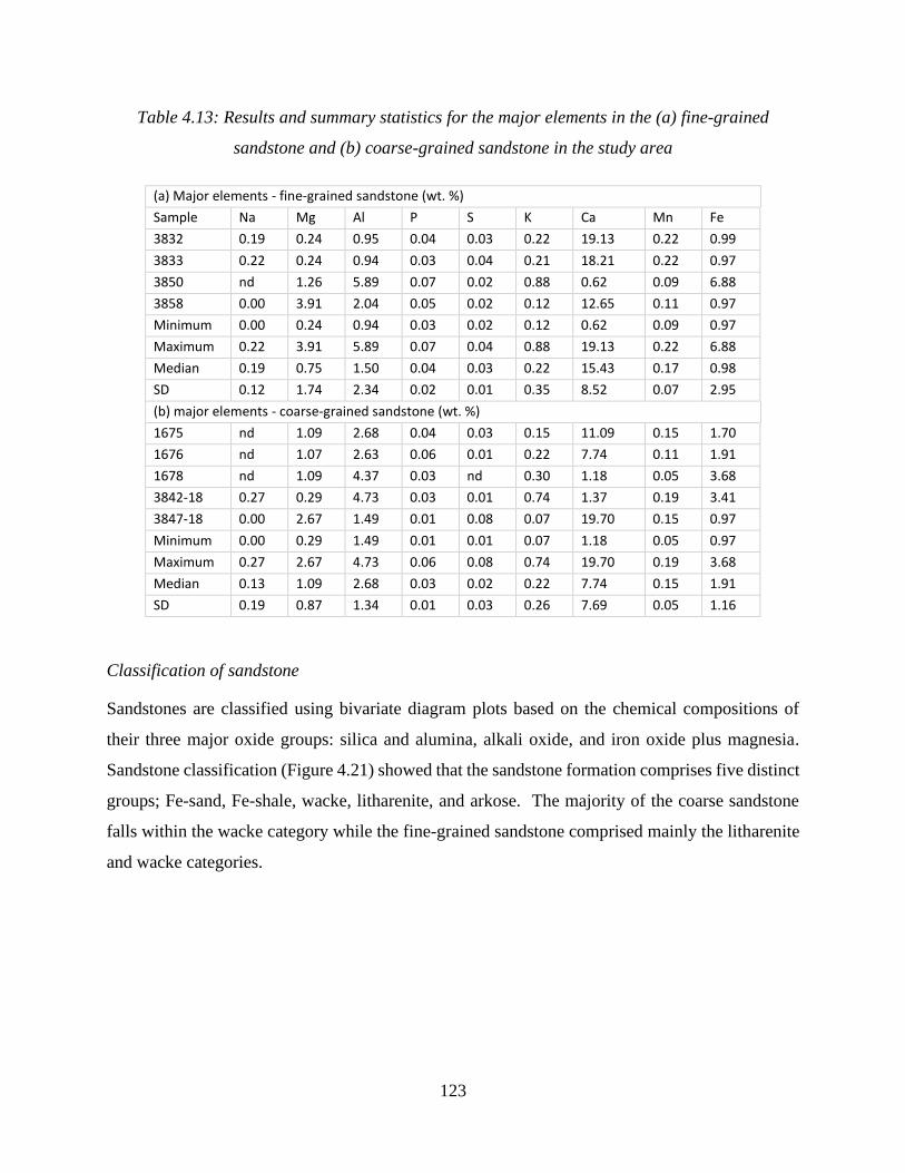
123

Table 4.13: Results and summary statistics for the major elements in the (a) fine-grained

sandstone and (b) coarse-grained sandstone in the study area

(a) Major elements - fine-grained sandstone (wt. %)

Sample Na Mg Al P S K Ca Mn Fe

3832 0.19 0.24 0.95 0.04 0.03 0.22 19.13 0.22 0.99

3833 0.22 0.24 0.94 0.03 0.04 0.21 18.21 0.22 0.97

3850 nd 1.26 5.89 0.07 0.02 0.88 0.62 0.09 6.88

3858 0.00 3.91 2.04 0.05 0.02 0.12 12.65 0.11 0.97

Minimum 0.00 0.24 0.94 0.03 0.02 0.12 0.62 0.09 0.97

Maximum 0.22 3.91 5.89 0.07 0.04 0.88 19.13 0.22 6.88

Median 0.19 0.75 1.50 0.04 0.03 0.22 15.43 0.17 0.98

SD 0.12 1.74 2.34 0.02 0.01 0.35 8.52 0.07 2.95

(b) major elements - coarse-grained sandstone (wt. %)

1675 nd 1.09 2.68 0.04 0.03 0.15 11.09 0.15 1.70

1676 nd 1.07 2.63 0.06 0.01 0.22 7.74 0.11 1.91

1678 nd 1.09 4.37 0.03 nd 0.30 1.18 0.05 3.68

3842-18 0.27 0.29 4.73 0.03 0.01 0.74 1.37 0.19 3.41

3847-18 0.00 2.67 1.49 0.01 0.08 0.07 19.70 0.15 0.97

Minimum 0.00 0.29 1.49 0.01 0.01 0.07 1.18 0.05 0.97

Maximum 0.27 2.67 4.73 0.06 0.08 0.74 19.70 0.19 3.68

Median 0.13 1.09 2.68 0.03 0.02 0.22 7.74 0.15 1.91

SD 0.19 0.87 1.34 0.01 0.03 0.26 7.69 0.05 1.16

Classification of sandstone

Sandstones are classified using bivariate diagram plots based on the chemical compositions of

their three major oxide groups: silica and alumina, alkali oxide, and iron oxide plus magnesia.

Sandstone classification (Figure 4.21) showed that the sandstone formation comprises five distinct

groups; Fe-sand, Fe-shale, wacke, litharenite, and arkose. The majority of the coarse sandstone

falls within the wacke category while the fine-grained sandstone comprised mainly the litharenite

and wacke categories.

124

Figure 4.21: Sandstone classification diagram after Herron (1988)

(d) Conglomerate – Specimens 1677 and 3857

The mineralogical compositions of two specimens of conglomerate collected at Lodwar town

(1677) and Natir area (3857) were as follows; SiO2 ranged was 60.07% for sample 1677 and

71.60% for sample 3857. There was no significant variation in Al2O3 (1677 = 9.72 and 3857

(9.15%) and that of Fe2O3 (1677=2.03 % and 3857 = 2.51%) (Figure 4.22). The conglomerate at

Natir had higher CaO (12.15%) as compared to that at Lodwar town (4.99 %). Similarly, LOI

(8.68%), K2O (3.52%), Na2O (1.7%), and MnO (0.70%) were also higher in this formation. In

terms of minor elements, Ca was relatively higher (14.86%) for the conglomerate at Natir than in

Lodwar town (2.63%) and is believed to be derived from the underlying Turkana grits. Mg (2.20%)

was also observed to be higher in sample 3857 than in specimen 1677 (1.08). Al, Fe, and Ti were

observed to be slightly higher in specimen 1677 than in specimen 3857, while there were no

significant variations in P, S, K, Cr, Ni, Cu, Zn and Mo with concentrations <0.05%.

125

Figure 4.22: Variations of major and trace elements in the conglomerate at Lodwar town (1677)

and Natir area (3857)

(e) Grainstone

Generally, slight variations were observed in the compositions of major elements in Grainstone

except for CaO that was relatively higher (23.00 %) in the fine-grained sample (1657). The coarse-

grained grainstone had higher levels of SiO2 (64.30%), Al2O3 (8.30%), MgO (5.19%), K2O

(2.19%), and Na2O (0.73%) than in medium-grained grainstone; SiO2 (58.07%), Al2O3 (5.80 %),

MgO (0.02%), K2O (1.06%), and Na2O (0.20%) (Figure 4.23). Occurrence of minor elements in

the medium-grained grainstone was as follows; Ca =17.18%, Al = 1.37%, Fe = 1.22%, Mg =

0.43%, Mn =0.41% and K = 14%. The compositions of Na, P, S, Cr, Ni, Zn, Se and Mo ranged

from <0.01 to 0.05% while Ti, Cu, As and Pb were not detected limits in the rock samples.

0

10

20

30

40

50

60

70

80

SIO

2

Al2

O3

CaO

MgO

Na2

O

K2

O

TiO

2

Mn

O

Fe2

O3

LOI

Na

Mg Al P S K C

a Ti Cr

Mn Fe Co Ni

Cu Zn As

Se Mo

Pb

Co

mp

osi

tio

ns

(%)

Conglomerate -1677 Conglomerate -3857

126

Figure 4.23: Variations in compositions of major elements in Grainstone samples

(iii) Volcanic rocks

(a) Nepheline-phonolites

SiO2 in the nepheline-phonolite ranged from 48.24 to 54.81 % with the specimen that formed a

contact with the Turkana grit (1653) having the highest silica content. The nepheline-phonolite at

contact zone also had the highest compositions of Al2O3 (15.31 %), CaO (8.20 %) and K2O (2.50

%). Slight variations in the Fe2O3 content were observed with values ranging from 9.61 to 10.08%.

The rock samples also had low Na2O (0.90 -1.28 %) and MnO (0.16 - 0.70 %) compositions as

compared to the rest of the oxides (Figure 4.24). The occurrence of the minor and trace elements

was determined for specimen 1650 of the nepheline-phonolite and the Turkana grit sample at

contact zone (1653). As a result, S, As, and Pb were not detected while Mg was determined to be

1.37% at the contact zone. Fe (3.62-6.01 %), Al (3.87 - 5.46 %), and Ca (1.69 - 6.80 %) were the

most abundant minor elements, followed by K (0.52 -0.87 %), Ti (0.10- 0.71 %), P (0.08 - 0.33

%) and Mn (0.13 - 0.20%). Concentrations <0.01 to 0.02% were observed in Na, Cr, Co, Ni, Cu,

Zn, Se and Mo.

0

10

20

30

40

50

60

70

SIO2 Al2O3 CaO MgO Na2O K2O TiO2 MnO Fe2O3 LOI

Co

mp

osi

tio

ns

(%)

Medium-grained Grainstone - 1657 Coarse-grained Grainstone - 1667

127

Figure 4.24: Distribution of the major elements in the rock samples of the nepheline-phonolite at

Lodwar town, grit contact and at Kanamkemer

(b) Augite basalts

The analysis of the distribution of the major elements in the augite basalt was as follows; SiO2

(53.79 %), Al2O3 (18.00%), moisture and volatile materials (9.22%), Fe2O3 (6.08%), CaO (5.69%),

Fe (5.08%), Ca (4.99%), Al (4.70%), MgO (3.22%), K2O (2.06%), Mg (1.26%), and TiO2 (1.09%).

Fe (5.09%), Ca (4.99%), Al (4.70%), and Mg (1.26%) had significant concentrations of the minor

elements while K, P, and Mn were ranged from 0.17 to 0.48%. All the trace elements were 0.26%

in the augite basalt (Figure 4.25).

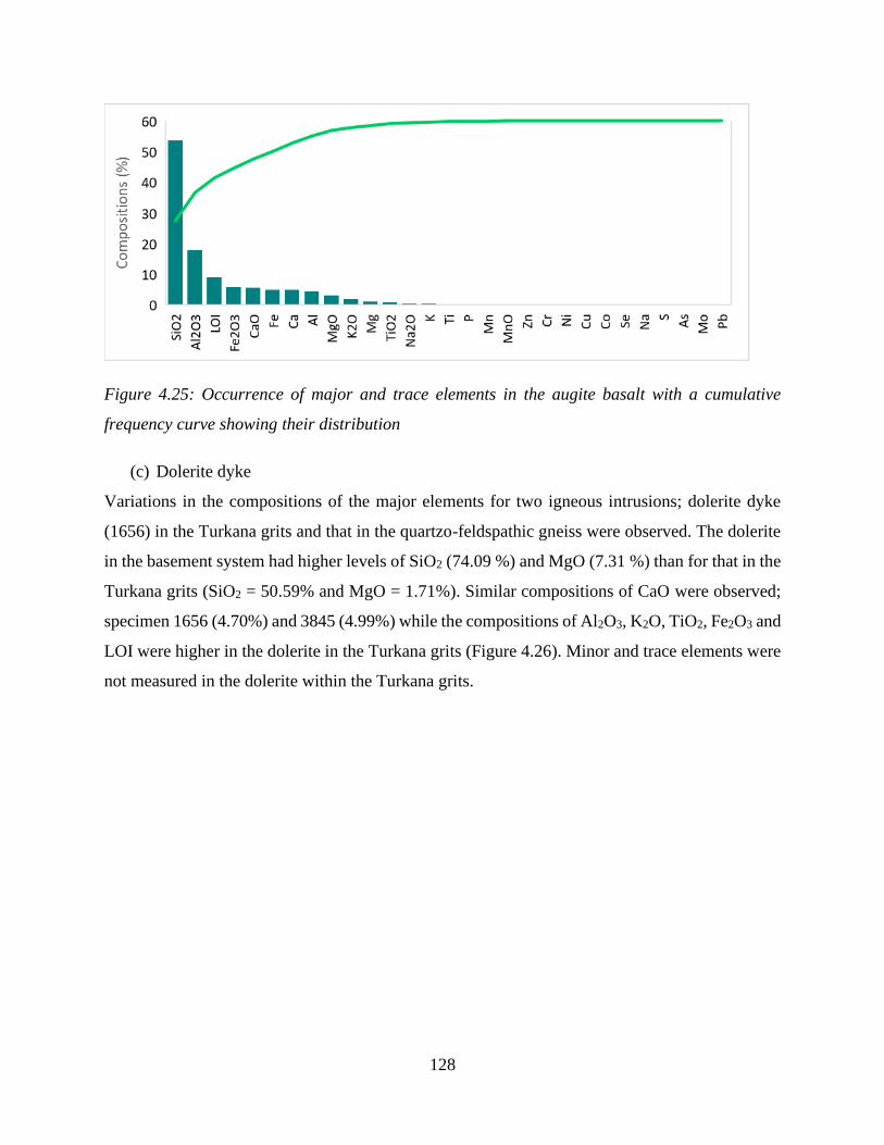
128

Figure 4.25: Occurrence of major and trace elements in the augite basalt with a cumulative

frequency curve showing their distribution

(c) Dolerite dyke

Variations in the compositions of the major elements for two igneous intrusions; dolerite dyke

(1656) in the Turkana grits and that in the quartzo-feldspathic gneiss were observed. The dolerite

in the basement system had higher levels of SiO2 (74.09 %) and MgO (7.31 %) than for that in the

Turkana grits (SiO2 = 50.59% and MgO = 1.71%). Similar compositions of CaO were observed;

specimen 1656 (4.70%) and 3845 (4.99%) while the compositions of Al2O3, K2O, TiO2, Fe2O3 and

LOI were higher in the dolerite in the Turkana grits (Figure 4.26). Minor and trace elements were

not measured in the dolerite within the Turkana grits.

129

Figure 4.26: Compositions of major elements in the dolerite dyke in the Turkana grits and in the

Basement system

Classification of Volcanic rocks

The TAS classification diagram (Figure 4.30) revealed that the nepheline phonolite at Lodwar

town and that forming contact with the Turkana grits belonged to basaltic-andesite group while

augite basalt and the nepheline phonolite at Kanamkemer area were identified to be volcanic

andesite. The intrusive rock was identified to be a dolerite of distinct volcanic origins; the dolerite

dyke in the Turkana grit was determined to be basaltic trachyandesite in nature while the intrusion

in the basement system identified to be dacite rock grading into rhyolite. The AFM classification

of the volcanic rocks in the study area based after Irvine and Baragar (1971) showed that augite

basalt and dolerite in the Turkana grit being cacl-alkaline while the nepheline-phonolite, and the

dolerite in the Basement system as tholeiitic in nature Figure 4.33.

130

Figure 4.27: TAS classification diagram for the volcanic rocks

131

Figure 4.28: AFM classification diagram After Irvine et al., 1971 showing augite basalt and

dolerite in the Turkana grit being cacl-alkaline while the nepheline-phonolite, and the dolerite in

the Basement system as tholeiitic in nature

4.2.1.5 Results of the Geophysical Survey

The results of the 26 vertical electrical soundings (VES) carried out in Sections A-D of the LAAS

aquifer are presented. Table 4.16 and Table 4.17 provide the field VES results, where VES 2 was

disregarded due to poor potential contact during the geophysical survey. A graph of apparent

resistivity (Ωm) against electrode spacing (m) was prepared for each of the VES points using

IP2WIN inversion software. The graph shows the number of layers (N), apparent resistivity value

(ρ), the thickness of the layer (h) and depth bgl (d).

LAAS Section A

Section A consists of the aquifer section west of the Lodwar municipality and north of the Turkwel

River, where four VES measurements were carried out (VES 17, 18, 19 and 20) with AB/2 of 200

m and five geoelectric layers were displayed (Appendix 4-12). The first layer had resistivity values

132

ranging from 24.40 to 100.00 Ohm-m and up to 3.75 m bgl while the second layer had resistivity

ranging between 136.00 to 183.00 Ohm-m to a depth of 12 m. The resistivity of the third layer

ranged from 17.00 to 28.70 Ohm-m at depths between 22.50 to 60.00 m, followed by a fourth layer

with low resistivity values of 3.95 to 13.00 Ohm-m at a depth of 25.00 – 160.00 m. The fifth

(bottom) layer had resistivity <10.00 Ohm-m at a depth >163.00 m, these readings were carried

out shortly after the long rains in May 2018 and, thus, the low resistivity values of the first top

layer and the second layer regarded as unsaturated sands. The third and the fourth layer are likely

to be saturated with fresh water while the resistivity of the fifth layer (< 10 Ohm-m) reflect saline

groundwater or clay. Pseudo-cross-section (Figure 4.29) shows resistivity distribution of the sub-

surface strata across VES 20, 18, and VES 19. The VES 20 was conducted in the area adjacent to

Turkana grits formation, and thus the huge disparity with VES 19, 18 and 17.

Figure 4.29: Pseudo-cross-section and resistivity cross-section between VES 18, 19 and 20 where

VES 17 was omitted from the pseudo section since it was not in the straight path with the three

selected points

133

LAAS Section B

Section B of the LAAS system covers the area west of the municipality of Lodwar and the south

of the Turkwel River, stretching from Kakemera to Nachomin areas where seven resistivity

measurements were performed (VES 13, 14, 15, 16, 23, 24 and 25). The results of the geophysical

survey indicated that four geoelectric layers underlie this section of the aquifer (Appendix 4-13).

Disparities were observed in the resistivity values of the top layer in this area up to a depth of 3.50

m; VES 16 and 23 had the lowest resistivity value of 17.70 and 23.20 Ohm-m attributed to the wet

top surface at the time of the survey. Moderate resistivity values between 53.00 to 86.40 Ohm-m

were recorded at VES 13, 15 and 24. Highest resistivity values (average = 256.60 Ohm-m) were

recorded at VES 14 and 25. The second layer had moderate resistivity values ranging from 29.8

to 39.8 Ohm-m at a depth of 4.30 at VES 16 and VES 23 and up to a depth of 16.00 m at VES 24.

This layer was not identified in VES 13 and 15, which were carried out in the adjacent Turkana

grits. The third layer had resistivity ranging between 17.00 and 79.40 Ohm-m and occurred at

varying depths, between 5.50 to 35.00 m to the east and between 6.50 to 100.00 m to the west of

the area., and can be associated with fresh groundwater in this section. The fourth layer had

resistivity 10 Ohm-m and interpreted to be an aquiclude (clay layer). Pseudo-sections were

prepared for VES 13, 15, 16, 23, and 24 to show the sub-surface resistivity distribution of rocks in

the area (Figure 4 30).

134

Figure 4.30: Pseudo-cross-section and resistivity cross-section between Kakemera (east) and

Nachomin (west) areas (VES 13, 15,16, 24, and 23)

LAAS Section C

Section C of the LAAS covered East of Lodwar municipality and north of the Turkwel River,

including Kakwanyang and Nang’omo areas. Only two vertical electrical soundings were carried

out in this section (VES 21 and 22) due to thick vegetation cover. Three layers were identified in

this section of the aquifer, where VES 21 had generally higher resistivities than VES 22. The first

layer had resistivity values between 62.69 and 140.00 Ohm-m, while the second layer had

moderate resistivity values from 36.10 to 56.30 Ohm-m up to a depth of 16 m. Below this layer

are resistivity values between 12.00 to 27.77 Ohm-m up to a depth > 100 m reflecting resistivities

of a saturated formation. A low resistivity layer of < 10 Ohm-m is believed to underlie this site

based on the observed trends of resistivity (Figure 4.31).

135

Figure 4.31: Pseudo-cross-section and resistivity cross-section of VES 21 and VEs 22 between

Kakwanyang and Nang’omo areas

LAAS Section D

Section D of the LAAS covers the area East of Lodwar municipality and south of Turkwel River,

including Napuu, Lolupe, and Nayuu areas. A total of 13 vertical electrical soundings were carried

out within a thin section (VES 1, VES 3 to VES 12, VES 26 and VES 27). More electrical

soundings were considered in this area than in other parts of the LAAS due to the large area and

increased groundwater abstraction observed (See Figure 3.4). The VES results in this section

revealed three distinct groups of electrical resistivities;

1) Group 1 comprised low to moderate resistivity values (VES 9, 10, 11, 12, and 26) and

were located in the Holocene sediments at Lolupe and Nayuu areas. The top layer had

average resistivity values between 50.00 and 130.00 Ohm-m to a depth of 2.50 m of

62.32. The second layer had medium resistivity values between 150.00 and 480.00 Ω

m while the third layer consisted of relatively lower resistivity values than the second

layer (18.00 and 35.00 Ω m) from depths ranging from 40 to 100 m and may be hosting

fresh groundwater between Lolupe and Nayuu areas. Resistivity values < 10.00 Ω m

underlie the area and may be clayey materials or saline groundwater.

136

2) Group 2 comprised VES 1, 3,4, 6 and 7 and were located in the Holocene sediments

adjacent to the Turkana grits in Lodwar (VES 1) and between Napuu and Lolupe areas

(VES 3, 4, 6 and 7). These VES points are characterised by medium to high resistivity

values (300 to 1070 Ohm-m) in the upper layer, 90 to 140 Ohm-m in the second layer

and while the third layer comprised resistivity values ranging from 25 to 65 Ohm-m

from 40 to 160 m, which is considered deeper than between Lolupe and Nayuu areas

(group 2). The fourth layer comprise resistivity values < 10 Ω m representing that of

clay layer or saline groundwater.

3) Group 3 comprised VES 5, 8 and 27 located in the Turkana grits and were

characterised by extremely high resistivity values (1260 to 3825.00 Ohm-m) in the

upper layers and very low resistivity values in the bottom layer (< 10 Ohm-m). The

middle layers had relatively high values between 200 to 800 Ohm (second layer)

followed by a third layer with resistivity values from < 10.00 and 70.00 Ohm-m. The

Turkana grit is highly consolidated and thus the high resistivities observed in this

formation. The low resistivity values recorded in this formation is associated with

saline groundwater.

Figure 4.32: Pseudo-cross-section from west to east of Section D of the LAAS (a) and from south

to north (b) toward the Turkwel River

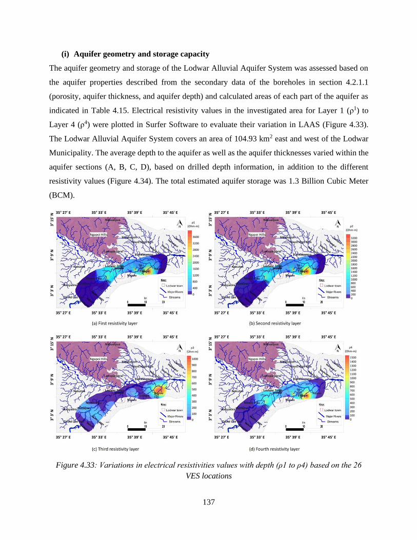
137

(i) Aquifer geometry and storage capacity

The aquifer geometry and storage of the Lodwar Alluvial Aquifer System was assessed based on

the aquifer properties described from the secondary data of the boreholes in section 4.2.1.1

(porosity, aquifer thickness, and aquifer depth) and calculated areas of each part of the aquifer as

indicated in Table 4.15. Electrical resistivity values in the investigated area for Layer 1 (ρ1) to

Layer 4 (ρ4) were plotted in Surfer Software to evaluate their variation in LAAS (Figure 4.33).

The Lodwar Alluvial Aquifer System covers an area of 104.93 km2 east and west of the Lodwar

Municipality. The average depth to the aquifer as well as the aquifer thicknesses varied within the

aquifer sections (A, B, C, D), based on drilled depth information, in addition to the different

resistivity values (Figure 4.34). The total estimated aquifer storage was 1.3 Billion Cubic Meter

(BCM).

Figure 4.33: Variations in electrical resistivities values with depth (ρ1 to ρ4) based on the 26

VES locations

138

Figure 4.34: Resistivity values of the inferred aquifer layer in the study area showing values <10

Ohm-m indicating possible saline groundwater

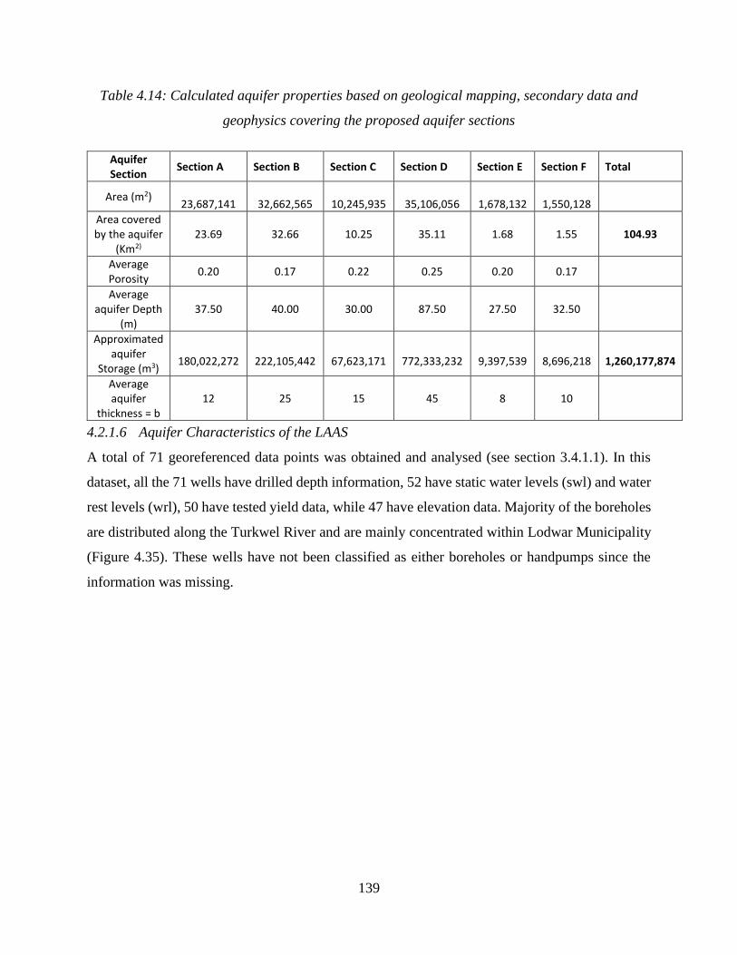
139

Table 4.14: Calculated aquifer properties based on geological mapping, secondary data and

geophysics covering the proposed aquifer sections

Aquifer Section

Section A Section B Section C Section D Section E Section F Total

Area (m2)

23,687,141

32,662,565

10,245,935

35,106,056

1,678,132

1,550,128

Area covered by the aquifer

(Km2) 23.69 32.66 10.25 35.11 1.68 1.55 104.93

Average Porosity

0.20 0.17 0.22 0.25 0.20 0.17

Average aquifer Depth

(m) 37.50 40.00 30.00 87.50 27.50 32.50

Approximated aquifer

Storage (m3)

180,022,272

222,105,442

67,623,171

772,333,232

9,397,539

8,696,218

1,260,177,874

Average aquifer

thickness = b 12 25 15 45 8 10

4.2.1.6 Aquifer Characteristics of the LAAS

A total of 71 georeferenced data points was obtained and analysed (see section 3.4.1.1). In this

dataset, all the 71 wells have drilled depth information, 52 have static water levels (swl) and water

rest levels (wrl), 50 have tested yield data, while 47 have elevation data. Majority of the boreholes

are distributed along the Turkwel River and are mainly concentrated within Lodwar Municipality

(Figure 4.35). These wells have not been classified as either boreholes or handpumps since the

information was missing.

140

Figure 4.35: Distribution of secondary data points in the study area with depth information - the

majority of shallow boreholes are along the Turkwel River and are mainly concentrated within

Lodwar town

(i) Aquifer depth

The drilled depth of boreholes ranged between 5.6 and 121.0 m below ground level. Boreholes

with a depth between 5.6 and 30.0 m are in the shallow aquifer (44), 31.0 to 100.0 m deep are in

the intermediate aquifer (23), while boreholes with depth > 100.0 m (four) are considered to be in

the deep aquifer (cf. Olago 2018). Thus, the majority of the wells (62%) tap the shallow aquifer

while the rest tap either the intermediate aquifer (32%) or the deep aquifer (6%). From Figure 4 -

141

14 above, it can be noted that the shallow boreholes are within the riparian zones of the Turkwel

River while deeper wells are located outwards.

(ii) Aquifer yield

Of the 71 boreholes in the study area obtained from the Water Resources Authority database, 51

had tested yield information as follows; 36 in the SA, 11 in the IA and three in the deep aquifer.

The yields of boreholes in the shallow aquifer (<30.0 m deep) ranged from 1.02 – 77.00 m3/h, 0.30

– 27.00 m3/h in the intermediate aquifer and between 45.00 to 100.00 m3/h in the deep aquifer.

The average yields of the wells in the shallow and intermediate aquifers were 16.87 m3/h and 8.28

m3/h, respectively. The yields of the three wells in the deep aquifer are as follows: Napuu Bh,

100.00 m3/h; Natir Bh, 8.00 m3/h and; borehole C5167, 4.5 m3/h.

(iii) Static water levels (swl) and water rest levels (wrl)

The water rest levels ranged between 1.0 and 22.0 m bgl in the shallow aquifer, 2.4 to 77.0 m in

the IA and between 3.5 to 62.0 m in the deep aquifer. The static water levels, on the other hand,

ranged from 0.7 to 17.0 m in the shallow aquifer, 1.1 to 19.1 m in the intermediate aquifer and 1.2

to 54.7 m in the deep aquifer. Thus, the piezometric surface is nearer to the surface in the shallow

aquifer, followed by the intermediate aquifer and then the deep aquifer.

(iv) Porosity and specific yield

Most studies regard the porosity of alluvium, which is a mixture of sand and gravel to be between

0.20 to 0.35 (Chilton and Seiler, 2006; Foster and Chilton, 2003; Okiongbo and Soronnadi-

Ononiwu, 2004). An average value of 0.27 was taken to represent the porosity of the shallow

alluvial aquifer, representing the porosity of both sand and gravel in the aquifer. The porosity of

the Turkana Grit Shallow Aquifer, intermediate aquifer and that of the deep aquifer was estimated

based on (Malvić et al., 2005), taking into account the different porosity of geological materials

(Table 4.15).

142

Table 4.15: Minimum and maximum porosity values of various geological materials based on

Todd, 1980

Aquifer type Formation Min Max

SAA Sand and gravel 0.20 0.35

TGSA Clayey gravels, clayey sandy

gravels 0.17 0.27

IA Fine medium sand 0.29 0.46

DA Silty or sandy clay 0.20 0.64

(v) Hydraulic conductivity

The aquifer material of the Lodwar Alluvial Aquifer System comprises of fine-medium sand with

hydraulic conductivity ranging between 2.0 x 10-7 m/sand 5.0 x 10-4 m/s. Thus, the average

hydraulic conductivity of the aquifer would be 1.14 x 10-5 m/s and equivalent of 1.22 m/day.

(vi) Transmissivity

Transmissivity of the boreholes in the study was calculated using Equation 3-12 for 44 boreholes

and handpumps with data on yield, static water level (swl) and water rest levels (wrl), where yield

is divided by drawdown, and the result is multiplied by the hydraulic conductivity. The hydraulic

conductivity used in the calculation was 1.22 m/day. The transmissivity of boreholes in the shallow

aquifer ranged from 2.99 and 2166.72 m2/day in the shallow aquifer, 0.31 to 608.12 m2/day in the

intermediate aquifer, and 10.98 to 1273.04 m2/day in the deep aquifer. Average transmissivity

values indicate that the deep aquifer in Napuu has a high groundwater potential (1316.11 m2/day),

followed by the shallow aquifer (440.00 m2/day) and then the intermediate aquifer (115.18

m2/day). It is important to note that majority of the boreholes in the study area have been drilled

in the shallow aquifer (Figure 4.36).

143

Figure 4.36: Spatial distribution of transmissivity values in the study area based on secondary

data obtained from the WRA database

(vii) Groundwater flow

Groundwater flow in an aquifer is governed by changes in gravity and hydraulic head. The

topography of an area determines the general direction of groundwater flow. In the study area, the

trend shown by the stream lineament is northwest to south-east north of Turkwel River and the

south-west to north-east south of Turkwel River. The surface run-off in the areas originates in from

the higher elevation volcanic and metamorphic terrains and passes through the Turkana grits into

the alluvial zones of the Turkwel River. Piezometric data of 52 boreholes and handpumps in the

study area were plotted in Surfer Software to determine the general groundwater flow direction.

The results revealed that the groundwater movement followed the general trend of the surface

water in the area with localized flow systems occurring in the southern portion of the river (Figure

4.37). Kuria (2013) has linked localized flow systems to a low local recharge.

144

Figure 4.37: Piezometric surface map of the study area determined from static water levels

Hydrogeochemistry and Water Quality

To characterise the aquifer hydrogeochemistry and its susceptibility to pollution borehole depth

information acquired from the secondary data was used. However, information on the drilled depth

of each handpump and borehole was not fully available. Drilled depth data was available for only

28 of the 53 observed handpumps (depth ranging between 5 – 45 m), with one recorded outlier at

75 m; 17 of these had depth less than 30 m below ground level, and therefore fall in the shallow

aquifer category (cf. Olago, 2018)—similarly, 22 of 41 observed boreholes, including all nine

LOWASCO production boreholes. The depth of these boreholes ranged from 17 to 110 m. Of

these, ten had depth between 17 and 30 m and were categorised as shallow alluvial aquifer (SAA),

including seven LOWASCO boreholes. Likewise, another set of ten borehole s had depth between

31 to 100 m and was in the intermediate aquifer (IA) while the remaining two had depth greater

than 100 m and are in the deep aquifer (DA) (cf. Olago 2018). In general, the number of sampled

sites without drilled depth information was 44 (25 handpumps and 19 boreholes) and have been

referred to in this study as “depth unknown” (DU). Of the 94 groundwater samples collected in

145

the wet season of May 2018, 58 were resampled in February 2019 dry season, where only 16

handpumps and 18 boreholes gad drilled depth information. With this regard, groundwater

chemistry in the LAAS has been evaluated in SAA, IA, DA and DU. Shallow aquifer located

outside the riparian zones of the Turkwel River has been identified as Turkana Grit Shallow

Aquifer (TGSA).

4.2.2.1 Physico-chemical properties

a) Turkwel River

The electrical conductivity (EC) of the Turkwel River had a small range of between 200.0 and

420.0 μS / cm, with a median value of 209.36.0 μS / cm (Table 4.16). The pH of the Turkwel River

samples was slightly alkaline, varying from 7.5 to 8.0; slightly less alkaline waters are noted to the

east of the Turkwel and Kawalase rivers confluence (Figure 2-1). The river water was quite warm,

with temperatures ranging from 30.6 °C to 36.1 °C, and was slightly cooler than the average high

temperature (about 38 °C) observed in the region during the sampling period. No clearly

discernible characteristics are observed in concentrations of cations from upstream to downstream,

except for Na, which rises considerably east of the confluence of the Turkwel and Kawalase rivers

(Figure 2-1). Relatively higher content of Fe and Mn occurred in all samples of the Turkwel River

except for sample 2437 where Mn was <0.01 mg/L, but with the highest level of Fe (2.76 mg/L).

No sulphate and nitrites were detected, while nitrate, chloride, and bicarbonate concentrations are

generally low.

146

Table 4.16: Physico-chemical results for samples collected in the dry season of February 2018

for the Turkwel River shaded fields are values that exceed guideline values for drinking water,

and 'nd' refers to not detected. The samples were arranged (left to right) from upstream to

downstream

Sample Code

2434 2435 2437 2438 2439 2440 2441 Min Max Median

EC 210 380 220 200 420 200 210 200 420 210.00

pH 8.65 7.70 8.82 9.11 8.92 8.73 9.53 7.70 9.53 8.82

Temp. 33.4 33.7 36.1 32.6 30.6 31.7 34.0 30.6 36.1 33.4

Turb. 311 228 154 549 96 834 521 96 834 311

Ca 25.60 25.60 26.40 25.60 24.00 26.40 24.80 24.00 26.40 25.60

Mg 6.33 7.79 5.36 7.79 8.76 7.30 7.30 5.36 8.76 7.30

Na 2.10 2.00 7.70 2.00 2.80 2.20 6.00 2.00 7.70 2.20

K 5.1 4.6 5.4 4.7 4.3 4.4 5.3 4.3 5.4 4.7

Fe 2.06 2.37 2.76 2.7 1.66 2.46 2.13 1.66 2.76 2.37

Mn 0.16 0.16 <0.01 0.16 0.12 0.16 0.2 0.12 0.2 0.16

HCO3 96.63 96.83 101.97 99.25 116.19 121.23 121.61 96.63 121.61 101.97

SO4 nd nd nd nd nd nd nd N/A N/A N/A

Cl 2 10 5 4 1 1 5 1 10 4

NO3 0.32 <0.01 0.37 0.86 0.17 <0.01 0.25 0.17 0.86 0.32

NO2 nd nd nd nd nd nd nd N/A N/A N/A

b) Groundwater – seasonal variations

(a) Shallow Aquifers

(i) Shallow alluvial aquifer (SAA)

The range of EC values in the shallow alluvial aquifer differed significantly between the dry and

wet seasons; the minimum EC values were roughly comparable (195-207 S / cm for the dry seasons

versus 210 S / cm for the wet season), but the EC maximum was three times higher in the wet

season than in any of the dry seasons (1857 μS / cm versus 630-632 μS / cm) (Table 17). Likewise,

although the pH level in the dry seasons was 7.60 to 8.22, in the wet seasonin the wet season, it

was higher, from 7.65 to 8.91. Besides, the maximum turbidity values in the wet season also show

a two- and five-fold increase as compared to each of the two dry seasons. Groundwater

temperatures ranged from 28.1 to 35.7°C.

147

The groundwater can be classified as non-saline in terms of chemistry except for the Napuu 1

borehole that was mildly saline in the dry season of February 2018, the only time it was tested.

With respect to the median concentrations of the cations in the SAA, Ca concentration is consistent

over the two-dry, and one wet season, Mg and K were depleted in the dry season in February 2019

compared to the dry season in February 2018 and the wet season in May 2018, and Na is

significantly depleted in the wet season relative to the two dry seasons. For the anions, the season

in February 2018 has the highest concentrations for HCO3, SO4 and Cl and the lowest

concentrations in the wet season in May 2018 while F concentrations are comparable in all three

seasons. The nitrate concentrations are generally low; February 2018 (0.03-0.68 mg N/L); May

2018 (0.02-0.54 mg N/L); and February 2019 (0.02-0.19). Ca (very low, Kakemera Primary

handpump – wet season May 2018), Na (high, BH7 – dry season February 2019), K (high, KFS

handpump – wet season May 2018) and SO4 (very high, BH7 – dry season February 2019; high,

Napuu 1, dry season February 2018) are noted as major site-specific anomalies.

148

Table 4.17: Physico-chemical parameters results during the February 2018 dry season for the SAA and IA (2452 and 2460); (the

shaded values exceed thedrinking water guidelines of KEBS (2014) and WHO (2011))

No Sample ID

Code EC pH Temp Turbidity Ca Mg Na K Fe Mn HCO3 SO4 Cl F NO3 NO2

Units µS/cm °C NTU Mg/L Mg/L Mg/L Mg/L Mg/L Mg/L Mg/L Mg/L Mg/L Mg/L MgN/L MgN/L

1 Bh 1A 2455 209 7.90 28.90 1.06 26.40 6.33 3.00 4.60 0.03 0.01 118.62 1.82 3.00 0.46 0.03 nd

2 Bh 1B 2454 220 7.60 28.10 0.17 28.00 7..31 2.00 4.40 0.17 0.01 123.95 3.41 2.00 0.47 nd nd

3 Bh 2C 2453 262 8.00 29.50 0.42 33.60 7.31 5.20 4.10 0.07 0.50 125.62 1.78 4.00 0.50 nd nd

4 Bh 3 2448 233 7.80 29.30 0.91 28.00 10.20 2.60 4.30 0.03 0.01 123.66 2.22 2.00 0.41 nd nd

5 Bh 5 2449 265 7.60 29.80 0.69 32.00 8.28 5.50 4.60 0.03 0.01 138.53 nd 5.00 0.44 nd nd

6 Bh 6 2444 561 8.20 34.20 0.36 20.80 1.31 100.00 4.00 0.03 0.01 230.58 19.00 28.00 0.45 0.16 0.02

7 Bh 6 2450 257 7.70 29.20 1.59 36.80 7.31 2.40 4.60 0.03 0.01 126.25 2.63 4.00 0.43 nd Nd

8 Bh 7 2445 207 7.90 28.80 1.01 25.60 5.85 5.00 4.00 0.10 0.01 99.25 2.69 2.00 0.39 0.20 Nd

9 Napuu 1 2451 1256 8.00 32.70 1.02 47.20 22.90 190.00 5.10 0.07 0.01 422.76 109.00 114.00 0.99 0.68 Nd

10 Napuu 4 2452 503 8.10 32.60 0.94 23.20 7.79 72.00 3.90 0.03 0.01 260.24 6.80 18.00 1.29 0.20 Nd

11 Nayuu Hp 2460 596 8.60 35.70 2.06 1.60 2.43 130.00 1.30 0.07 0.01 253.41 10.70 19.00 1.26 2.34 Nd

12 Lolupe Hp 2456 630 8.00 33.40 2.00 25.60 22.40 70.00 4.20 0.90 0.01 321.30 13.50 12.00 0.75 nd Nd

149

Table 4.18: Physicochemical parameters for the SAA in the wet season (shaded fields indicate values that exceed the guidelines for

drinking water)

No sample ID

Code EC pH Temp Turbidity Ca Mg Na K Fe Mn HCO3 SO4 Cl F NO3 NO2

Units µS/cm °C NTU Mg/L Mg/L Mg/L Mg/L Mg/L Mg/L Mg/L Mg/L Mg/L Mg/L MgN/L MgN/L

1 Akibululu Hp 3344 306 8.50 31.40 2.65 29.60 8.28 20.00 3.80 0.10 0.40 170.00 0.03 8.00 0.79 0.12 0.07

2 Bh 1A 3381 260 8.91 28.90 5.94 36.80 6.82 3.00 4.70 0.03 0.04 126.80 2.07 13.00 0.31 0.30 nd

3 Bh 1B 3380 240 8.64 29.80 0.03 26.40 7.79 4.00 4.90 0.03 <0.01 124.10 6.49 6.00 0.32 0.36 nd

4 Bh 2C 3382 310 8.21 30.40 3.30 34.40 9.25 8.00 4.30 0.07 0.50 156.10 2.70 12.00 0.31 0.15 nd

5 Bh 3 3383 240 8.45 30.00 0.43 28.00 8.76 3.00 4.70 >0.01 <0.01 121.50 2.73 6.00 0.29 0.06 nd

6 Bh 5 3387 270 8.32 29.90 1.87 33.60 7.79 3.00 4.70 0.03 0.08 160.50 2.00 5.00 0.32 >0.01 nd

7 Bh 7 3384 210 8.56 29.90 0.54 25.60 8.28 3.00 4.20 0.03 0.14 111.80 2.28 5.00 0.29 >0.01 nd

8 Bh 9 3388 260 8.35 28.70 0.66 29.60 11.68 3.00 4.50 0.03 <0.01 133.40 4.83 5.00 0.27 0.09 nd

9 Kakemera Pri Hp 3300 528 8.67 32.90 5.30 3.20 9.23 99.00 1.10 0.07 <0.01 259.40 9.15 12.00 0.93 0.21 nd

10 KFS Hp 3390 424 7.92 28.70 10.53 30.40 14.11 27.00 14.00 0.17 0.50 216.70 23.85 12.00 0.60 0.08 nd

11 Locher A Akalale Hp 3346 297 8.51 31.10 1.85 16.80 5.35 37.00 2.60 0.07 0.10 145.00 6.40 8.00 0.74 0.17 nd

12 Lodwar Mixed Pri 1 3355 353 7.84 30.30 8.05 29.60 6.82 32.00 2.90 0.03 0.20 180.40 2.77 8.00 1.68 0.04 0.02

13 Lodwar Mixed Pri 2 3356 332 7.65 31.80 1.23 34.40 8.77 18.00 3.70 0.03 0.60 159.80 4.22 11.00 1.08 0.07 nd

14 Lokipetot Bh 3329 380 8.32 29.00 5.15 24.80 16.05 29.00 4.30 >0.01 <0.01 218.70 6.36 1.00 0.56 0.14 nd

15 Lolupe 3 Hp 3360 594 8.05 34.40 1.41 27.20 11.68 80.00 4.30 >0.01 <0.01 341.60 7.37 12.00 0.81 0.04 nd

16 Nabulon water well 3365 236 8.36 31.30 0.29 28.00 4.88 10.00 4.40 0.07 <0.01 116.80 2.65 7.00 0.53 >0.01 nd

17 Nadapal Hp 3313 324 7.84 31.00 7.09 29.60 15.57 8.70 3.20 0.07 0.60 173.90 2.38 1.00 1.18 0.02 nd

18 Nakwalele Hp 2 3338 632 8.70 32.60 5.28 24.80 8.28 98.00 4.20 0.07 0.04 281.90 19.92 36.00 0.99 0.13 nd

19 Nakwamekwi Pri Bh 3307 270 8.33 29.70 5.12 26.40 12.16 6.00 3.50 0.03 <0.01 145.50 3.44 3.00 0.57 >0.01 nd

20 Naregai Bh 3312 350 8.35 32.80 4.51 20.80 18.96 20.00 5.70 0.07 <0.01 191.60 10.15 3.00 0.93 >0.01 nd

21 Nasenyanait Hp 2 3351 320 8.23 32.00 1.78 32.00 14.60 6.40 4.10 0.07 0.06 171.50 5.80 3.00 0.66 0.16 nd

22 Natotol 3354 271 8.18 30.20 6.05 28.00 9.74 9.00 4.10 0.17 0.60 138.00 1.03 2.00 0.63 0.54 nd

150

Table 4.19: Physico-chemical parameters for the SAA in the dry season (February 2019 - shaded values exceed the KEBS and WHO

guidelines for drinking water)

No. Sample ID

Code EC pH Turbidity Ca Mg Na K Fe Mn HCO3 SO4 Cl F NO3 NO2

Units µS/cm °C NTU Mg/L Mg/L Mg/L Mg/L Mg/L Mg/L Mg/L Mg/L Mg/L Mg/L MgN/L

1 Akibululu Hp 2256 360 7.95 1.20 33.60 5.85 32.00 2.70 0.07 0.60 195.89 3.70 9.00 0.51 0.11 nd

2 Bh 1A 2225 195 8.13 0.58 27.20 2.93 6.10 3.10 0.10 nd 103.52 1.10 15.00 0.44 0.02 nd

3 Bh 1B 2226 224 8.09 0.10 33.60 2.94 6.60 1.10 0.07 nd 125.33 2.26 nd 0.45 nd nd

4 Bh 2C 2227 241 8.13 4.92 40.80 0.51 6.90 1.00 0.13 0.60 146.85 1.55 4.00 0.57 0.05 nd

5 Bh 3 2263 228 8.00 0.49 32.00 4.39 6.00 2.00 0.07 nd 86.97 5.19 25.00 0.34 0.13 nd

6 Bh 5 2224 249 8.15 NIL 33.60 5.37 7.40 1.90 0.07 nd 120.30 3.83 5.00 0.52 nd nd

7 Bh 7 2269 1857 8.04 0.41 44.00 0.03 375.00 3.20 0.10 0.12 205.15 721.00 5.00 0.33 0.04 nd

8 Bh 9 2223 309 8.10 0.22 31.20 2.45 30.00 2.80 0.07 nd 139.76 5.88 29.00 0.50 0.03 nd

9 Kakwanyang Dispensary Bh

2258 280 8.08 0.85 33.60 3.91 17.00 3.10 0.10 nd 156.71 4.39 2.00 0.41 0.19 nd

10 Lodwar Mixed Pri 1 2249 403 8.18 0.36 39.20 5.37 40.00 1.40 0.07 nd 218.72 3.84 8.00 1.62 0.10 nd

11 Lolupe 3 Hp 2214 496 8.20 1.26 31.20 1.96 75.00 2.40 0.03 nd 283.42 5.87 4.00 1.16 nd nd

12 Nadapal Hp 2233 392 8.15 0.68 18.40 8.76 50.00 1.10 0.07 1.20 218.94 2.16 14.00 1.18 0.07 nd

13 Nakwamekwi Pri Bh 2237 239 8.22 0.06 33.60 6.34 3.00 2.30 0.07 nd 144.00 1.02 1.00 0.56 0.02 nd

14 Naregai Bh 2264 387 8.11 0.80 25.60 16.05 30.00 4.10 0.07 nd 183.08 10.60 3.00 0.22 nd nd

15 Nasenyanait Hp 2 2251 256 8.15 0.40 40.00 1.48 8.20 3.10 0.07 nd 144.36 6.62 nd 0.63 0.07 nd

151

(ii) Turkana Grit Shallow Aquifer (TGSA)

Data are available for the TGSA for one dry season (February 2019) and one wet season (May

2018) (Table 4.20). There were few handpumps targeting this aquifer, presumably as a result of

its moderately saline water. There are no significant variations between the dry and wet seasons in

the EC, except for the Bokotom hand pump. In general, however, the EC range for the shallow

groundwater of the Turkana grit was marginally lower in the wet season (3410 to 6840 μS/cm)

compared to the dry season (5170 to 8260 μS /cm). As in the case of the shallow alluvial aquifer,

whereas the minimum pH values were more or less the same (8.35 versus 8.40), the maximum pH

for this aquifer was markedly higher in the wet season (9.28) than in the dry season (8.68), and the

maximum turbidity difference between the dry seasons (7.64 NTU) and the wet seasons (20.86

NTU) was about three-fold. Temperature, recorded only in the wet season, ranged from 33.1 to

36.9 ° C, suggesting that the TGSA is warmer overall than the shallow alluvial aquifer.

The concentrations of Na, Cl and HCO3 are much higher as compared to the shallow alluvial

aquifer, and in most instances, the concentrations of all three parameters exceed 1000 mg/L each.

Also notable are: (i) the amounts of Ca in TGSA are lower than in SAA; and (ii) the concentrations

of SO4, F, and NO3 are far higher than in SAA. Contrasts between the dry and wet seasons in

TGSA relate to (i) higher median concentrations of Mg, SO4, F and NO3 in the wet as compared

to the dry season, except for the Loyo Primary handpump where the reverse is observed, and (ii)

relatively lower median values of Cl in the wet season (685.00 mg/L) as compared to the dry

season (830.50 mg/L). However, comparison of Cl concentrations for individual wells between

the wet and dry seasons showed a reverse trend for some wells.

152

Table 4.20: Physico-chemical parameters for the TGSA during the wet and dry seasons (shaded values exceed the KEBS (2014) and

WHO (2011) guidelines for drinking water)

Turkana Grit Shallow Aquifer (TGSA)- Dry season (February 2019)

No Sample ID

Code EC pH Temp. Turb. Ca Mg Na K Fe Mn HCO3 SO4 Cl F NO3 NO2

Units µS/cm °C NTU Mg/L Mg/L Mg/L Mg/L Mg/L Mg/L Mg/L Mg/L Mg/L Mg/L MgN/L MgN/L

1 Talent High

Sch Hp 2252 5600 8.56 nm 7.64 3.20 1.46 1280.00 1.20 0.27 nd 941.73 350.00 1120.00 9.60 7.81 nd

2 Bokotom

Hp 2253 8260 8.40 nm 1.24 8.00 17.98 1850.00 3.10 0.07 nd 492.68 268.00 2395.00 2.19 3.27 nd

3 Loyo Pri Hp 2266 5170 8.68 nm 1.38 4.80 0.49 1182.00 2.70 0.10 nd 1769.51 351.60 446.00 17.24 5.03 nd

4 Trumpet of

Hope Ministries

2267 5570 8.82 nm 0.86 0.80 0.49 1280.00 2.30 0.10 nd 1773.54 388.00 541.00 12.28 7.82 nd

Turkana Grit Shallow Aquifer (TGSA)- Wet season (May 2018)

Sample ID Code EC pH Temp. Turb. Ca Mg Na K Fe Mn HCO3 SO4 Cl F NO3 NO2

5 Talent High

Sch Hp 3331 6370 9.06 35.70 12.70 4.80 2.92 1453.00 2.60 0.27 nd 1407.19 426.00 1020.00 10.41 19.81 nd

1 Namuthia

Hp 3333 3410 9.12 36.00 20.86 4.00 2.92 770.00 1.50 0.67 nd 828.27 207.03 525.00 3.09 7.15 nd

3 Bokotom

Hp 3334 6840 8.35 36.90 4.26 12.00 18.04 2020.00 2.90 nd nd 492.38 610.00 2390.00 2.22 4.76 nd

6 Trumpet of

Hope Ministries

3394 5340 9.28 35.40 6.74 <1.00 0.49 1226.00 2.70 0.17 nd 1333.31 608.06 500.00 15.31 33.64 nd

2 Al Noor

Community 3396 6270 8.62 33.10 1.10 9.60 13.60 1400.00 5.10 0.10 nd 1215.15 934.60 780.00 18.74 1.34 nd

4 Loyo Pri Hp 3399 5190 8.79 33.50 4.56 2.40 1.95 1190.00 3.70 0.03 nd 1602.75 324.71 590.00 18.67 7.92 nd

153

(iii) Intermediate Aquifer (IA)

Data for this aquifer is available for the two dry and one wet season but for the first dry season of

February 2018 are limited to only two samples. Based on the EC, the groundwater is mainly non-

saline in the intermediate aquifer, but there are some slightly saline pockets. Compared to the SAA,

although in both dry and wet seasons the minimum EC values were similar, the EC average was

higher in the wet season, but not considerably higher than in the SAA. The pH range was wider in

the wet season (7.61-9.76) than in the dry season (8.10-8.67). Furthermore, similar to the SAA and

TGSA, the average turbidity in the wet season was far higher than in the dry season, and a seven-

fold increase is observed in this aquifer for the maximum turbidity values in the wet season

compared to the dry season. The groundwater temperature range is 31.3 to 36.0 ° C, broadly

comparable to the TGSA.

The median concentration values of Ca, Mg, K, HCO3, SO4 and Cl in this aquifer are higher in the

wet season compared to the dry season, and much more so particularly for Mg and SO4. More

generally, the concentration ranges for the measured cations and anions in the wet season are wider

and more variable in the wet than in the dry season.

154

Table 4.21: Results for the intermediate aquifer physico-chemical parameters in the wet season (the shaded fields are values that

exceed guideline values for drinking water of KEBS (2014) and WHO (2011)

No Sample ID

Code EC pH Temp Turbidity Ca Mg Na K Fe Mn HCO3 SO4 Cl F NO3 NO2

Units µS/cm °C NTU Mg/L Mg/L Mg/L Mg/L Mg/L Mg/L Mg/L Mg/L Mg/L Mg/L MgN/L MgN/L

1 Bh 6 3389 590 8.33 32.9 0.75 20 14.6 76 4.4 0.03 0.04 281 25 25 0.35 0.3 nd

2 Chokochok Pry 3341 929 7.77 33.4 3.77 32 42.3 93 4.7 nd 0.6 327 20.9 118 0.84 0.14 0.07

3 Chukultom Hp 3386 888 9.28 35.3 2.03 1.6 7.77 186 2.6 0.03 nd 337 47.1 93 0.67 0.17 0.04

4 Comboni Girls 3398 1220 9.58 33.6 0.16 nd 1.46 272 1.6 0.03 nd 383 73.7 140 1.41 0.57 0.05

5 Eleleia Pri Hp 3364 1557 9.59 35.7 1.44 4 12.2 330 1.1 0.1 nd 812 29.9 25 4.58 0.37 nd

6 Kakemera Chr 3302 1308 7.61 35 6 42.4 24.8 203 2.7 0.07 nd 758 15.7 24 1.25 0.2 nd

7 Kochoda Hp 3391 850 9.76 33.9 2.17 nd 3.89 187 1.2 0.1 nd 437 22.2 15 1.62 0.15 nd

8 Limyounsim Bh 3309 1673 7.93 34.7 4.72 56 13.2 227 6.4 0.07 nd 701 41.2 44 1.43 1.08 nd

9 Loporkou-

Eleleai Hp 3366 914 9.52 35.3 1.3 nd 2.43 205 1.3 0.07 nd 383 36.5 57 1.64 3.45 nd

10 Nachomin Bh 3306 1060 8.48 36 4.15 6.4 4.86 188 1.5 0.03 nd 498 23.1 3 2.24 0.54 nd

11 Nadapal Supply 3314 750 7.76 32.6 4.65 20.8 35.5 86 3.2 0.1 0.12 446 12.3 13 0.95 nd nd

12 Nagis Bakhita 3317 520 7.98 33.5 4.08 24.8 22.9 53 2.6 0.07 nd 296 12.2 20 0.14 nd nd

13 Nakwamekwi 3310 805 9.33 34.5 5.1 nd 5.34 174 1.4 0.07 nd 394 31.1 26 0.95 0.66 nd

14 Napuu 2 3373 370 8.9 32 1.01 15.2 8.27 44 3.6 0.07 nd 199 5.13 4 0.77 1.17 nd

15 Napuu 3374 520 8.52 32 0.48 24 10.2 63 4.3 0.07 nd 264 14.4 2 0.81 0.37 nd

16 Nareng'elup 2 3323 1040 7.86 33.8 49.28 45.6 73.9 45 0.2 0.5 nd 512 41.6 22 2.01 3.71 0.23

17 Natot Pri Bh 3357 370 8.68 31.3 1.18 25.6 12.7 33 3 0.03 nd 208 6.53 4 1.55 nd nd

18 Nauren Puu 3392 600 8.2 34 0.2 16 9.73 91 4.2 0.03 nd 335 9.55 16 0.86 0.07 nd

19 Nayuu Hp 4 3368 820 8.56 34.5 2.32 8.8 6.81 164 2.9 0.2 nd 384 32.5 61 0.48 2.1 nd

20 Nayuu Hp

Resample 3363 650 9.3 35.4 1.17 0.8 1.94 144 1.4 0.1 nd 317 20.5 21 0.97 2.44 nd

155

Table 4.22: Results for the intermediate aquifer measured water quality parameters of February 2019 (the shaded values exceed

thedrinking water guidelines of KEBS (2014) and WHO (2011))

No Sample ID Sample

ID EC pH Turbidity Ca Mg Na K Fe Mn HCO3 SO4 Cl F NO3 NO2

µS/cm NTU Mg/L Mg/L Mg/L Mg/L Mg/L Mg/L Mg/L Mg/L Mg/L Mg/L MgN/L MgN/L

1 Chukultom Hp 2228 736 8.56 nd 7.2 0.98 160 1.1 0.07 nd 283 35 62 1.56 0.13 nd

2 Eleleia Pri Hp 2216 906 8.67 0.49 nd 0.97 206 0.2 0.03 nd 396 32.1 50 2.15 3.07 nd

3 Kakemera Church 2222 1182 8.18 7.12 39.2 22.4 180 0.9 0.23 nd 661 11.3 538 1.75 0.15 nd

4 Nachomin Bh 2217 1025 8.41 0.33 9.6 1.95 220 1.7 0.1 nd 547 22.8 15 2.85 0.29 nd

5 Nadapal Supply

bh 2234 510 8.29 0.1 16.8 8.27 80 1.5 0.07 0.2 275 7.49 10 1.14 0.02 nd

6 Nakwamekwi Hp 2230 678 8.63 nd 4 0.97 150 0.4 0.04 nd 302 26.3 29 1.05 0.63 nd

7 Napuu 2 2246 420 8.24 0.55 22.4 2.93 65 2.4 0.07 nd 240 1.15 3 0.88 0.76 nd

8 Napuu 4 Resample 2245 614 8.23 nd 24.8 8.76 100 2.3 0.03 nd 312 16.9 21 0.71 0.17 nd

9 Nareng'elup 2 2261 1051 8.11 4.49 21.6 31.6 160 2.8 0.27 nd 624 24.7 nd 0.77 1.71 nd

10 Natot Pri Bh 2244 375 8.36 0.66 26.4 11.7 35 1.9 0.03 nd 203 7.31 4 1.72 <0.01 nd

11 Nauren Puu 2235 545 8.24 nd 18.4 8.76 86.3 1.8 0.07 nd 285 9.08 14 1.54 nd nd

12 Nayuu Hp 2211 607 8.55 0.59 4.8 nd 135 0.7 0.1 nd 309 19.6 14 1.23 2.14 nd

13 Nayuu HP4 2212 813 8.41 0.45 15.2 1.47 170 1.2 0.2 nd 338 33.9 55 0.69 1.79 nd

156

(iii) Deep Aquifer

There are no marked differences in the physico-chemical parameters for each of the two deep

borehole sites in the wet-dry season, suggesting recharge occurs over time scales longer than

the seasonal cycles. The Natir borehole is non-saline while the Napuu 1 borehole is slightly

saline, but the two have fairly similar pH, temperature, and turbidity values, as well as

concentrations of Ca, K, and Fe (Table 4.23). The concentrations of Ca in the DA are similar

throughout the seasons compared to the SAA, and IA. During dry season generally, the

concentrations of Mg and Na in Napuu 1 Bh are similar to those of the IA while in Natir Bh

are in the range of observed values in the SAA in the dry season.

Table 4.23: Water quality parameters for the deep aquifer during the dry and wet seasons

(highlighted values exceed the KEBS (2014) and WHO (2011) guideline value for drinking

water)

Sample ID Napuu 1 Natirnalulung Bh (Natir)

Sample Code 2451 2210

Parameters Feb-18 May-18 Feb-19 May-18 Feb-19

EC 1256 1250 1392 320 273

pH 8.00 8.30 8.12 8.63 7.95

Temperature 32.70 33.00 N 32.00 N

Turbidity 1.02 1.06 0.15 1.46 1.37

Ca 47.20 22.40 36.00 36.00 33.60

Mg 22.87 25.28 24.32 7.80 5.85

Na 190.00 203.00 230.00 11.50 11.20

K 5.10 5.70 3.10 4.80 3.00

Fe 0.07 0.03 0.07 0.03 0.07

Mn 0.01 nd nd nd nd

HCO3 422.76 495.27 553.88 145.67 125.76

SO4 109.00 69.08 81.40 8.41 6.29

Cl 114.00 111.00 110.00 19.00 13.00

F 0.99 0.83 0.95 0.42 0.50

NO3 0.68 0.71 0.42 0.15 4.69

NO2 nd nd nd nd nd

Seasonal variation of groundwater chemistry

(i) Physical parameters

Seasonal variations of major cations and anions are given in Figure 4.38. Figure 4.38a shows

a decreasing trend of EC in aquifers in the wet season, with the TGSA recording the highest

EC values. Figure 4.38b shows slightly alkaline pH in the wet season than in the dry season

across the aquifers. The SAA is observed to be cooler than the TGSA, IA and the DA. High

157

turbidity is observed in the TGSA in wet and dry seasons while turbidity in the SAA, IA and

DA is observed to be relatively higher in the wet season (Figure 4.38c).

Figure 4.38: Seasonal variations in the physico-chemical parameters in the river warer

(RW), shallow alluvial aquifer (SAA) intermediate aquifer (IA), Turkana Grit Shallow

Aquifer (TGSA) and the deep aquifer (DA)

(ii) Major cations

Na+ concentration was observed to be higher in the dry season as compared to in the wet season

in shallow and deep aquifers, where the Turkana grit shallow aquifer had the highest

concentrations of Na+ during the wet and dry seasons (Figure 4.39a). The intermediate aquifer

had higher Na+ in the wet season compared to in the dry season. Ca2+ concentration was higher

in the SAA and in the DA in the dry season but higher in the TGSA and in the IA in the wet

season (Figure 4.39b). Mg2+ was generally higher in the wet season across all the groundwater

samples where significantly higher concentrations were observed in the Turkana grit shallow

aquifer (Figure 4.39c). The K+ was also higher across all the aquifers in the wet season (Figure

4.39d). The Fe2+ of the river water was relatively higher than the shallow and intermediate

aquifers, which had higher increased concentrations of Fe2+ in the wet season due to existence

of oxidising an environment (Figure 4.3e)

158

Figure 4.39: Seasonal variations in the major cations in the river water (RW), shallow

alluvial aquifer (SAA) intermediate aquifer (IA), Turkana Grit Shallow Aquifer (TGSA) and

the deep aquifer (DA)

(iii) Major anions

The concentrations of HCO3- increased across all the aquifers in the wet season with the

Turkana Grit shallow aquifer having concentrations > 492 mg/L during the wet and dry seasons

(Figure 4.40a). Precipitation of mineral phases such as calcite in the dry season may result in

decreased concentration of HCO3 in groundwater in the dry season. The Cl- in the shallow

alluvial aquifer slightly increased in the wet season (median = 6.50 mg/L) compared to a

median value of 4.0 in the dry season. Turkana grit aquifer had high Cl- levels with a median

value of 685.0 mg/L in the wet season and a median value of 830.50 mg/L in the dry season.

Dilution of chloride salts was observed in this aquifer in the wet season. The Cl- concentration

in the intermediate aquifer was 18.20 during the wet and dry season (Figure 4.40b).

159

The SO42- concentrations in the shallow and intermediate aquifer were observed to increase in

the wet season (Figure 4.40c). However, their levels did not exceed the acceptability values for

drinking water. Significantly high SO42- concentration was observed in the TGSA in the wet

season (median = 517.0 mg/L) and in the dry season (median = 350.8 mg/L). The SO42- in the

deep aquifer increased in the dry season possible from rock dissolution. NO3- concentration

increased in all the aquifers in the wet season with the TGSA having the highest concentrations

in dry and wet seasons (Figure 4.40d). Generally, F- concentrations increased in the dry season

in all the aquifers (Figure 4.40e). NO2- was detected in few samples of the shallow alluvial

aquifer and the intermediate aquifer in the wet season with concentrations higher than the

guideline value of 0.1 mg/L in the wet season (Figure 4.40f).

Figure 4.40: Seasonal variations in the major annions in the river water (RW), shallow

alluvial aquifer (SAA) intermediate aquifer (IA), Turkana Grit Shallow Aquifer (TGSA) and

the deep aquifer (DA)

160

c) Groundwater – spatial variations

Spatial changes in the physicochemical properties (EC, pH, and temperature) of the LAAS

indicated a variety of interesting characteristics (Figure 4.41). The lowest EC values are in

wells along the profile of the Turkwel River, in alluvial sediments of the Holocene epoch, and

where there are and ephemeral and seasonal feeder streams. The Turkana grits and the Miocene

nepheline-phonolites are correlated with the highest EC values, though their outcrops are

sometimes obscured by Quaternary deposits. The lowest groundwater pH (acidic waters) and

temperature are recorded next to the Turkwel River and its corresponding tributaries, while the

alkaline waters is associated with groundwater in the Turkana grits and the nepheline phonolite

zones. Higher turbidity in the wet season within both of the shallow aquifers and in the

intermediate aquifer is attributed to the remobilisation of clay and silt minerals by recharge

water. Another notable characteristic was the progression of rising Na+ and Cl- concentrations

from the shallow alluvial aquifer, through the intermediate aquifer to the Turkana Grit and vice

versa for Ca2+ and Mg2+.

161

Figure 4.41: Spatial variation of the physicochemical parameters (EC, PH, temperature and

turbidity) for the river water (RW), shallow alluvial aquifer (SAA) intemediate aquifer (IA),

Turkana Grit Shallow Aquifer (TGSA) and the deep aquifer (DA)

4.2.2.2 Hydrochemical facies

Four water types were identified from the study area's surface water and groundwater samples

using the Piper diagram (Figure 4.42a): Na-HCO3, Ca-HCO3, Na-Cl, and Mg-HCO3. All of the

surface water samples are Ca-HCO3 water.. The Ca-HCO3 water type dominates the shallow

alluvial aquifer (59%) followed by the Na-HCO3 water type (29%), and four samples had Mg-

HCO3 water type (12%). The Na-HCO3 water type of the shallow alluvial aquifer is observed

at Lolupe, Nakwalele, and Kakemera areas within the Holocene sediments. The TGSA at its

contact with the Holocene sediments has Na-HCO3 water type, while within the grit formation

proper it is 44% Na-Cl water type. The intermediate aquifer is almost entirely Na-HCO3 water

type (95%) except for Katapakori and Narengelup handpumps that belong to the Mg-HCO3

water type (12%). Mg-HCO3 water type occurs in isolated areas such as Akwanga, Nakadukui,

and Naregai. The Napuu and Natirnalulung boreholes of the deep aquifer belong to Na-HCO3

and Ca-HCO3, respectively.

162

The hydrochemical facies varies seasonally, for example, 55% of the dry season Na-HCO3

water type transitions to Ca-HCO3 in the wet season due to mixing with recharge waters (Figure

4.42b). Seven observations were made from sixteen groundwater samples that showed changes

in water facies between wet and dry season (Table 4.24):

(i) Na-HCO3 type water of the dry season becomes recharged with Ca-HCO3 type

water (3307, 3313, 3362 and 3367) and Mg-HCO3 type water (3312 and 3322) in

the wet season;

(ii) Some of the recharge water reaches the intermediate aquifer in the dry season

(February 2019) changing the water type from Na-HCO3 to Ca-HCO3 (3299, 3310,

3346) and to Mg-HCO3 type (3321, 3361, and 3371);

(iii) Some of the fresh groundwater becomes saline in the dry season (3302), indicating

seasonal aquifer mineralization;

(iv) Increased sulphate concentration in the dry season (3384) is linked to dissolution of

gypsum (calcium sulphate);

(v) Mg-HCO3 water type of the wet season may be altered to Ca-HCO3 water type in

the dry season (3323 and 3343); and

(vi) Na-Cl water type does not change seasonally (3331, 3334, and 3400).

163

Figure 4.42: Groundwater and surface water piper diagram (a) in the wet season and in (b)

the dry season

Table 4.24: Groundwater samples with variations in hydrochemical facies between the wet

and the dry season

S/No Sample Code May 2018

(Wet Season) February 2019 (Dry season)

1 3299 Na-HCO3 Ca-HCO3

2 3302 Na-HCO3 Na-Cl

3 3307 Ca-HCO3 Na-HCO3

4 3310 Na-HCO3 Ca-HCO3

5 3312 Mg-HCO3 Na-HCO3

6 3313 Ca-HCO3 Na-HCO3

7 3321 Na-HCO3 Mg-HCO3

8 3322 Mg-HCO3 Na-HCO3

9 3323 Mg-HCO3 Ca-HCO3

10 3343 Mg-HCO3 Ca-HCO3

11 3346 Na-HCO3 Ca-HCO3

12 3361 Na-HCO3 Mg-HCO3

13 3362 Ca-HCO3 Na-HCO3

14 3367 Ca-HCO3 Na-HCO3

15 3371 Na-HCO3 Mg-HCO3

16 3384 Ca-HCO3 Na-SO4

164

Figure 4.43: Changes in 58 groundwater samples collected in the wet season (May 2018)

and in the dry season (February 2019) in the hydrochemical facies

4.2.2.3 Groundwater quality Index (GWQI) and its seasonal variations

The groundwater quality indices (Figure 4.44, 45-; Table 4.25) for both the wet and dry seasons

were evaluated based on the ratings given in Table 3.13 (section 3.42). The results revealed

that the SAA is characterised by excellent (WQI = 0-25) to good (WQI = 26-50) quality water

during the wet and dry seasons except for seven samples in the wet season; two with poor water

quality (WQI = 51-75) and five with very poor water quality (WQI = 76-100). In the dry season,

one sample of the SAA had poor water quality while two samples had very poor water quality

index. The TGSA groundwater had a water quality index > 200 in both seasons and is

considered unsuitable for drinking. The intermediate aquifer is characterised by good

groundwater quality in the wet and dry seasons except for water sources adjacent to the Turkana

grit that had poor drinking water quality (WQI = 51-75). The deep aquifer also had good

drinking water quality. In the wet season, the majority if the boreholes and handpumps with

unknown depth had good drinking water quality (22 samples), poor water quality (seven), very

poor water quality (six), and unfit for drinking (nine). The water quality index of these

boreholes and handpumps (DU category) ranged between excellent quality in the dry season

(13 samples), good water quality (two), poor water quality (three), and very poor water quality

80 60 40 20

20 40 60 80

20

40

60

80

20

40

60

80

20

40

60

80

20

40

60

80

Ca Na+K HCO3+CO3 Cl

Mg SO4

<=Ca + Mg

Cl +

SO

4=>

Feb_2019

May_2018

Feb_2019

May_2018

165

(six). Generally, the WQI of groundwater in the study area was observed to improve in the dry

season (Table 4.25), suggesting possible flushing of pollutants and mineral dissolution in the

aquifers in the wet season. Excellent groundwater quality means that none of the assessed

parameters exceeded the KEBS (2014) and WHO (2011) drinking water guidelines, whereas

poor water quality means that one or more parameters exceeded the guideline. It was also found

that water samples with WQI greater than 100 had more than five chemical parameters in

excess of the guideline values.

Table 4.25: Water quality index (a) in the wet season and (b) in the dry season for the SAA,

IA, TGS and the DA, and for the boreholes and handpumps with an unknown depth

(a) WQI wet season

WQI Range

Type of water SAA TGSA IA DA Depth

Unknown Total

Samples %

Samples

<25 Excellent 6 Nil 1 Nil Nil 7 7.4%

26-50 Good 9 Nil 11 2 22 44 46.8%

51-75 Poor 2 Nil 6 Nil 7 15 16.0%

76-100 Very poor 5 Nil 1 Nil 6 12 12.8%

>100 Unfit for drinking Nil 6 1 Nil 9 16 17.0%

Total 22 6 20 2 44 94 100.0%

(b) WQI dry season

WQI Range

Type of water SAA TGSA IA DA Depth

Unknown Total

Samples %

Samples

<25 Excellent 9 Nil Nil Nil 13 22 37.9%

26-50 Good 2 Nil 9 2 2 15 25.9%

51-75 Poor 1 Nil 4 Nil 3 8 13.8%

76-100 Very poor 2 Nil Nil Nil 6 8 13.8%

>100 Unfit for drinking 1 4 Nil Nil Nil 5 8.6%

Total 15 4 13 2 24 58 100.0%

166

Figure 4.44: Variations in the water quality index values during the (a) wet season and in the

(b) dry season showing improved water quality in all the aquifers in the dry season

Figure 4.45 WQI map for the study area based on the 94 groundwater samples of the wet

season

167

4.2.2.4 Determination of processes affecting groundwater quality by a multivariate

statistical approach

PCA and HCA were carried out on the sample’s shallow alluvial aquifer, Turkana grit shallow

aquifer and on samples of the intermediate aquifer during the wet and dry seasons except for

the deep aquifer whose samples were insufficient for application of statistical techniques.

1) Principal Component analysis

(a) Shallow alluvial aquifer

The PC1 and PC2 for shallow alluvial aquifer contributed 33.0% and 20.2 % respectively of

the total variance in the wet season while the PC 1 and PC 2 in the dry season contributed

28.8% and 19.0%, respectively. Most of the chemical parameters loaded positively on PC 1

and PC 2 during the wet (Figure 4.46a) and majority loaded negatively on PC 1 and PC 2. In

the dry season, there was an enrichment of PC 1 variables in the groundwater leading to the

addition of K, Fe and Mn. The positive factors of PC1 in the wet season for the shallow alluvial

aquifer reflected changing ionic strength on the concentrations of EC, Na, Mg and HCO3 as a

result of dilution by recharge water.

(b) Turkana grits shallow aquifer

In the wet season, the PC1 and PC2 for Turkana grit shallow aquifer contributed 49.8% and

25.8 % respectively of the total variance while the PC 1 and PC 2 in the dry season contributed

68.7% and 17.9% respectively. pH, HCO3, F, and NO3- were loaded positively on PC 1 and PC

2 in the wet season (Figure 4.46c) and in the dry seasons (Figure 4.46d), where only NO3-

became negatively loaded in the dry season. EC, Ca2+, Mg2+, Na+ and Cl- were loaded

negatively on PC 1 in both seasons. The positive factors of PC1 in the wet season reflect

chemical concentrations controlled mainly by pH (EC, Na, Mg, HCO3, SO4, Cl and NO3). The

negative variables of PC 1 in this aquifer were Ca, Fe and Mn in the dry season with the

enrichment in the dry season leading to the addition of K, Mg and F.

(c) Intermediate aquifer

In the wet season, the PC1 and PC2 for intermediate aquifer contributed 30.2% and 23.6 %

respectively of the total variance while the PC 1 and PC 2 in the dry season contributed 33.8%

and 32.8% respectively. PC 1 during the wet and dry seasons was negatively loaded for most

chemical parameters, while PC 2 was positively loaded for most chemical parameters in both

seasons (Figure 4.46e, f). As in the case of the SAA, the positive factor loadings of PC1 in the

168

intermediate aquifer reflects changing ionic strength as a result of dilution by recharge water.

However, pH influences the positive chemical variables of PC1 in this aquifer and subsequent

addition of Fe to this PC. The negative members of PC 1 were Ca, K, Mn and NO3 reflecting

leaching of these ions from the soil zone. In the dry season, the reverse role of pH was observed,

and mineral enrichment leads to the addition of Ca and K to the positive factor loadings of PC

1. Ion exchange processes reflected by positive variables of PC 2 in the wet season involved

Ca and Mg carbonates leading to low pH, and this characteristic was reversed in the dry season.

The negative factor loadings in the wet season were Na, K and Cl reflecting salt dissolution

influencing changes in pH while the negative factor loadings in the dry season included Ca,

Mg, K and Mn indicating carbonate precipitation.

(d) Depth unknown

In the wet season, the PC 1 and PC 2 for the groundwater samples with unknown depths

contributed 39.7% and 19.7% of the total variability respectively. In the dry season, the PC 1

and PC 2 for these samples contributed 57.0% and 11.9% of the total variance. Majority of the

chemical parameters were positively loaded on PC 1 and PC 2 in the wet season (Figure 4.46g)

and in the dry season (Figure 4.46h). Positive PC1 factors for these samples in the wet season

represented dilution by recharge water and subsequent enrichment of EC, Na, K, Cl, and F in

this PC in the dry season. In the dry season, the positive factors of PC 2 indicated rock-water

interaction influenced by pH changes and leaching of Ca, Mg, K and Fe from the soil zone as

indicated by the negative variables of PC 2.

169

Figure 4.46: Factor loadings for PC 1 and PC 2 during (a) wet season and during (b) dry

season for the SAA; TGSA (c) wet season and during (d) dry season; IA during (e) wet season

and during (f) dry season and for the wells without the drilled depth information (g) wet

season and during (h) dry season

170

2) Hierarchical Cluster Analysis

The HCA was carried out for groundwater samples of the study area using the Microsoft Excel

add-in module XLSTAT 2019 utilizing group average clustering and euclidean distance

methods based on dissimilarities. Based on HCA, the groundwater samples of the study area

can be classified under two major groups; Group 1 (bicarbonate) and Group 2 (Sodium

chloride) water. The degree of mineralisation controlled by EC, Na, SO4 and Cl determines the

varied clusters in each group. In the wet season (Figure 4.47a), Cluster 1 (C1) of Group 1

consisted all samples (22) of the SAA, eight samples of the IA, two samples of the deep aquifer

and 32 samples with an unknown depth. Cluster 2 (C2) on the other hand, indicated increased

mineralisation from Cluster 1 (C1) with only two samples of the intermediate aquifer while the

rest had unknown depth value. Cluster 3 (C3) represented moderately to highly mineralised

groundwater as a result of mixing between the groundwater of the Holocene sediments and that

of the Turkana grit. In the dry season (Figure 4.47b) C1 of Group 1 consisted two sub-groups;

Ca-HCO3 water of the shallow alluvial aquifer and the Na-HCO3 water of the intermediate

aquifer, with each sub-group incorporating samples with an unknown depth. Cluster 2 (C2) of

Group 1 represented moderately mineralised groundwater in the transition zone between the

Holocene sediments and the Turkana grits. Clusters C3 and C4 are members of Group 2

representing highly mineralised groundwater of the Turkana grit shallow aquifer with C4 being

the Bokotom Hp which was more mineralised due to excess Na and Cl concentrations.

171

Figure 4.47: Dendrogram (a) in the wet season and (b) in the dry season for groundwater

samples, showing three main clusters in the wet season and four main groups in the dry

season, based on aquifer mineralization levels

3) Mineral saturation indices

The SI of the minerals in the SAA were undersaturated in the wet season while aragonite,

calcite, dolomite and manganese compounds showed saturation in the dry season (Figure

4.48a). In the wet season, the mineral SI was undersaturated except for the manganese

TGSA IA IA

TGSA IA IA

TGSA IA IA

TGSA IA IA

TGSA IA IA DU

DU

DU IA IA DU

DU

DU

DU IA DU

DU

DU

DU

DU

DA

DU

DU

DU IA IA

SA

AS

AA

DU

SA

AS

AA

DU

DU

SA

AS

AA

SA

AD

US

AA

SA

AS

AA

SA

AS

AA

SA

AS

AA

DU

DA

SA

AD

US

AA

SA

AS

AA

SA

AD

UD

UD

UD

UD

UD

UD

US

AA

DU IA IA

SA

A IA DU

DU

DU

SA

AD

UD

UD

UTG

SA IA IA DU

DU

DU

DU

DU

DU

DU

DU

DU

0

1000

2000

3000

4000

5000

6000

Dis

sim

ilari

ty(a) Dendrogram (Wet season)

Group 1Group 2

C1 C2C3

Sub-group 1Sub-group 2

DA

SAA

SAA

SAA

SAA

SAA

SAA

SAA

DU

DU

DU

SAA

SAA IA DU

SAA

SAA

SAA IA

SAA

SAA

DU IA DU IA DU IA IA DU IA IA DU

DU

DU IA IA DU IA DU IA DU

DU

DU

DU

DU

DU

SAA

DU

DU

DU

DA IA

TGSA

DU

DU

TGSA

TGSA

TGSA

0

1000

2000

3000

4000

5000

6000

Dis

sim

ilari

ty

(b) Dendrogram (Dry season)

Group 1

Group 2

C1 C2

C3C4

Sub-group 2Sub-group 1

172

compounds and saturated in the dry season with respect to aragonite, calcite, dolomite and

hausmannite (Figure 4.48b). Apart from aragonite, calcite, dolomite and manganese

compounds, the SI of the rest of the minerals were undersaturated in the intermediate aquifer

during the wet and dry seasons (Figure 4.48c). The SI of the minerals in the deep aquifer was

undersaturated during the wet and dry seasons except for aragonite, calcite and dolomite

(Figure 4.48d). The SI of the minerals for the wells with unknown depth was undersaturated in

the wet season and saturated for aragonite, calcite, dolomite and manganese compounds in the

dry season (Figure 4.48e).

173

Figure 4.48: Saturation indices of minerals in the wet season (May) and in the February -

dry season for (a) SAA; (b) TGSA; (c) IA; (d) DA and wells without drilled depth

information

-30-25-20-15-10

-505

10152025

An

hyd

rite

(Ca

SO4

)

Ara

goni

te (C

aCO

3)

Calc

ite

(CaC

O3)

Do

lom

ite

(CaM

g(C

O3)

2)

Flu

orit

e (C

aF2)

Gyp

sum

(CaS

O4

:2H

2O)

Mel

ante

rite

(FeS

O4

:7H

2O

)

Sid

erit

e (F

eCO

3)

Hal

ite

(NaC

l)

Sylv

ite

(KC

l)

Rho

doch

rosi

(MnC

O3)

Pyro

lusi

te (M

nO

2:H

2O)

Pyro

chro

ite

(Mn

(OH

)2)

Man

gani

te (M

nO

OH

)

Hau

sman

nite

(Mn3

O4)

SI v

alu

es

SAA (May) SAA (Feb)

(a)

-10

-5

0

5

10

15

20

25

Anh

ydri

te (

CaSO

4)

Ara

goni

te (C

aCO

3)

Calc

ite

(CaC

O3)

Do

lom

ite

(CaM

g(C

O3

)2)

Flu

orit

e (C

aF2)

Gyp

sum

(CaS

O4

:2H

2O)

Mel

ante

rite

(Fe

SO4

:7H

2O

)

Sid

erit

e (F

eCO

3)

Hal

ite

(NaC

l)

Sylv

ite

(KC

l)

Rh

od

och

rosi

(Mn

CO

3)

Pyro

lusi

te (M

nO

2:H

2O)

Pyro

chro

ite

(Mn

(OH

)2)

Man

gani

te (M

nO

OH

)

Hau

sman

nite

(Mn3

O4

)

SI v

alu

es

TGSA (May) TGSA (Feb)

(b)

-15

-10

-5

0

5

10

15

20

25

Anh

ydri

te (

CaSO

4)

Ara

goni

te (C

aCO

3)

Calc

ite

(CaC

O3

)

Do

lom

ite

(CaM

g(C

O3)

2)

Flu

orit

e (C

aF2)

Gyp

sum

(CaS

O4

:2H

2O)

Me

lan

teri

te (F

eSO

4:7

H2

O)

Sid

erit

e (F

eCO

3)

Hal

ite

(NaC

l)

Sylv

ite

(KC

l)

Rho

doch

rosi

(MnC

O3)

Pyro

lusi

te (M

nO

2:H

2O)

Pyro

chro

ite

(Mn

(OH

)2)

Man

gani

te (M

nO

OH

)

Hau

sman

nite

(Mn3

O4)

SI v

alu

es

IA (May) IA (Feb)

(c)

-20.00

-15.00

-10.00

-5.00

0.00

5.00

An

hyd

rite

(C

aSO

4)

Ara

goni

te (C

aCO

3)

Calc

ite

(CaC

O3)

Do

lom

ite

(CaM

g(C

O3

)2)

Flu

ori

te (

CaF

2)

Gyp

sum

(CaS

O4:

2H2O

)

Mel

ante

rite

(FeS

O4:

7H2O

)

Sid

erit

e (F

eCO

3)

Hal

ite

(NaC

l)

Sylv

ite

(KC

l)

Rho

doch

rosi

(MnC

O3)

Pyro

lusi

te (M

nO

2:H

2O)

Pyr

och

roit

e (M

n(O

H)2

)

Man

gani

te (M

nO

OH

)

Hau

sman

nite

(Mn3

O4)

SI v

alu

es

DA (May) DA (Feb)

(d)

-25-20-15-10

-505

10152025

Anh

ydri

te (

CaSO

4)

Ara

goni

te (C

aCO

3)

Ca

lcit

e (

Ca

CO

3)

Do

lom

ite

(CaM

g(C

O3)

2)

Flu

orit

e (C

aF2)

Gyp

sum

(CaS

O4:

2H2O

)

Mel

ante

rite

(FeS

O4:

7H2O

)

Sid

erit

e (F

eCO

3)

Hal

ite

(NaC

l)

Sylv

ite

(KC

l)

Rho

doch

rosi

(MnC

O3)

Pyr

olu

site

(Mn

O2

:H2

O)

Pyro

chro

ite

(Mn

(OH

)2)

Man

gan

ite

(M

nO

OH

)

Hau

sman

nit

e (

Mn

3O

4)

SI v

alu

es

Depth Unknown (May) Depth Uknown (Feb)

(e)

174

4.2.2.5 Rock-water interactions in the LAAS

a) General aspects

The results presented in the sections above allow for investigation of the primary rock-water

interactions in the LAAS both generally and also in relation to the four different aquifer sub-

systems. The TGSA had the greatest Na+ concentrations followed by those with unknown

depths, then the intermediate aquifer and lastly those in the shallow alluvial aquifer. All the

groundwater and the surface water of the study region demonstrated a linear relationship with

a slope similar to-1 during the wet and dry seasons. Thus, this plot reveals that Na+, Ca2+ and

Mg2+ participate in ion change processes where dissolved Ca2+ and Mg2+ are exchanged with

adsorbed Na+ in the aquifer matrix. Figure 4.12 suggests that ion exchange is a major

hydrochemical process indicated by the slope, which is close to -1 (Fisher and Mullican, 1997).

The hierarchical cluster analysis (Figure 4.10) revealed that the groundwater of the study area

belongs to three major clusters in the wet season and four major clusters in the dry season based

on levels of mineralization in the aquifer systems. The relationship between Na+ and Cl- ions

in the groundwater formed similar clusters observed in the HCA results. The minerals

determined by the PHREEQC from the groundwater of the study area during the dry and the

wet seasons included; anhydrite, aragonite, calcite, dolomite, fluorite, gypsum, melanterite,

siderite, halite, sylvite, rhodochrosite, pyrolusite, pyrochroite, manganite, and hausmannite

mineral phases.

b) Contrasts in the LAAS Sub-systems

(i) Variations in Na+ and Cl- ions

The Na+/Cl- ratios of the shallow alluvial aquifer in the wet season were less or equal to 1.0 for

31.8% of the samples while the rest had ratios greater than one (Figure 4.49). In the dry season,

only two boreholes; Bh 1A and Bh 3 had Na+/Cl- ratios <1.0 while the rest (86.7%) had ratios

>1. All Turkana grit shallow aquifer samples had Na+/Cl- ratios greater than 1.0 in the wet

seasons (Figure 4.49a) and dry (Figure 4.49b), except for the Bokotom Hp, the ration of which

was equivalent to one in both seasons. All the groundwater samples of the intermediate aquifer

during the wet and dry seasons had Na+/Cl- ratios more significant than one except for

Chokochok Pri Hp that had a molar ratio of 1.2 in the wet season (Figure 4.49a) and that of

Kakemera Church Hp whose ratio was 0.5. The progression in Na+ concentration suggests that

many of the Bh/Hp with unknown depth are in the transition areas between the Holocene

sediments and the grit areas. The Na+/Cl- ratio for the wet season was 2.83 compared to that of

175

the dry season, which was 2.75, indicating that some of the Na+ are remobilized into solution.

Deep aquifer (DA) – Natirnalulung Bh of the deep aquifer had Na+/Cl- a ratio of 0.9 in the wet

season and 1.3 in the dry season while that of Napuu 1 Bh was 2.8 in the wet season and 3.2 in

the dry season (Figure 4.49). Wells with Unknown depth – Only two of the boreholes and

handpumps with no depth records had Na+/Cl- ratios less or equal to one in the wet season;

Nakadukui Bh (0.80) and Nasenyanait Hp (1.3) (Figure 4.49). In the dry season, only

Nakoporor Hp had a Na+/Cl- ratio of 0.7.

Figure 4.49: Plots for Na+/Cl- in groundwater in the (a) wet season and (b) dry season and

for the relationship between [Ca2+ + Mg2+ - SO42- - HCO3

-] and [Na+ - Cl-] (c) and (d) in the

surface water, shallow alluvial aquifer (SAA), intermediate aquifer (IA), Turkana grit

shallow aquifer (TGSA) and the deep aquifer (DA) (Fisher and Mullican, 1997)

-40

-35

-30

-25

-20

-15

-10

-5

0

5

-10 0 10 20 30 40 50

Ca2+

+ M

g2+-S

O42-

-H

CO

3-(m

eq

/l)

Na+ - Cl- (meq/l)

Deep aquiferDepth UnknownIntermediate AquiferShallow AquiferShallow aquifer gritTurkwel River

0

10

20

30

40

50

60

70

80

0 20 40 60 80 100

Cl- (

me

q/l

)

Na+ (meq/l)

Deep aquiferDepth UnknownIntermediate AquiferShallow AquiferShallow aquifer gritBokotomTurkwel River

0

10

20

30

40

50

60

70

80

0 20 40 60 80 100 120

Cl-(m

eq

/l)

Na+ (meq/l)

Deep AquiferDepth UnknownIntermediate AquiferShallow AquiferShallow aquifer gritBokotomTurkwel River

-40

-35

-30

-25

-20

-15

-10

-5

0

5

10

-10 0 10 20 30 40 50

Ca2+

+ M

g2+ -

SO42-

-H

CO

3-(m

eq

/l)

Na+ - Cl- (meq/l)

Deep AquiferDepth UnknownIntermediate AquiferShallow AquiferShallow aquifer gritTurkwel River

(a) Wet season (b) Dry season

(c) Wet season (d) Dry season

176

(ii) Hydrogeochemical process in aquifers

Dilution by recharge water occurs both in the SAA and IA related to changing ionic strength

in dry and wet seasons based on common behaviour of factor loadings on PC 1. The

undersaturation and saturation of aragonite, calcite and dolomite in the SAA controls the factor

loadings on PC 1 and PC 2 during the wet and dry seasons. while the saturation of these

minerals control PC1 and PC 2 of the IA. Other processes in this aquifer include; Ion exchange

processes reflected by positive variables of PC 2, leaching of ions (Ca, K, Mn and NO3) soil

zone, dissolution and carbonate precipitation motivated by reserves role of pH in the wet and

dry seasons, respectively. HCA revealed Natir Bh of the deep aquifer exhibits similar

characteristics with the SAA while that of Napuu Bh reflects the behaviour of the intermediate

aquifer. The positive factor loadings of PC 1 for wells with unknown depth are related to an

undersaturation of aragonite, calcite, dolomite and manganese compounds. Dilution by

recharge water, mineral dissolution and iron exchange were identified to the dominant

processes for these wells based on factor loadings of PC 1 and PC 2. Rock water interaction

in the wet season and increased mineral enrichment in the dry season from weathering and

release of Na, Ca, Mg, K, Mn, in the aquifer medium to the groundwater are the major processes

in the TGSA.

The groundwater of the SAA belonged to Cluster 1 (C1) sub-group 1, characterized by low

mineralization during the wet and dry season, as shown by the HCA (Figure 4.47). The HCA

revealed that two factors influence the groundwater chemistry of the intermediate aquifer in

the wet and dry seasons; (1) the proximity to the Turkwel river (Cluster C1) and (2) proximity

to the Turkana grits formation (C2 and C3) (Figure 4.47). The groundwater chemistry of the

TGSA is displayed as a unique system disconnected from the SAA, IA and the DA. The HCA

revealed highly mineralized groundwater in the TGSA belonging to Cluster 3 (C3) during the

wet and dry season with Bokotom Hp forming Cluster 4 (C4) in the dry season, owing to its

excess Na+ and Cl- ions. The HCA of the samples during the wet and dry seasons revealed that

the majority of the boreholes and handpumps with unknown drilled depth (32) belonged to the

shallow alluvial aquifer (Cluster 1), 12 in the intermediate aquifer while only two were in the

Turkana grit formation.

177

4.2.2.6 Aquifer vulnerability to pollution from point and diffuse sources; anthropogenic

pollution (results)

(a) Nitrate loading in river water

Nitrate loading in the Turkwel River was evaluated for the seven water samples collected in

the dry season of February 2018; two upstream samples (SW/006 and SW001), three within

the Lodwar Municipality ((SW/002, SW/007, and SW/005), and two samples (SW/004 and

SW/008) were located downstream (Figure 3.16). Samples located inside the municipal

boundary showed elevated NO3 levels Figure 4.50).

Figure 4.50: Nitrate levels across the Turkwel river samples indicating elevated levels for the

samples within the Lodwar Municipal boundary in the dry season of February 2018.

(b) Vulnerability of municipal groundwater sources to pollution

NO3 in 25 groundwater sources within the Lodwar municipality boundary showed increased

concentrations in the wet season. Although these concentrations were generally below the

guideline value of drinking water, institutional groundwater sources showed values

approaching the guideline values in the wet and dry season (Table 4.26). Generally, increased

NO3 concentrations were observed within the shallow alluvial aquifer than in the intermediate

aquifer and may be linked to leaching of NO3 ions from domestic wastewater (point sources)

and surface runoff (non-point sources).

SW/006 SW/001 SW/002 SW/007 SW/005 SW/004 SW/008

NO3 0.17 0.32 1 1 0.86 0.37 0.25

0

0.2

0.4

0.6

0.8

1

1.2

Nit

rate

(m

gN/L

)

West of Lodwar(Upstream)

Inside Lodwarmunicipality

East of Lodwar(Downstream)

178

To establish the water sources exposed to either point and non-point pollution sources, the

high-resolution DEM acquired from the drone mapping was used to extract the drainage

lineaments of the Lodwar municipality. The NO3 concentrations within the municipality

boundary were used to generate heatmaps based on natural breaks algorithm for identification

of point and non-point source pollution. The distribution of NO3 in groundwater of Lodwar

town is in the range of 0.01 to 0.37 mg N/L for most wells in the wet season and between 0.01

and 0.29 mg N/L in the dry season (Figure 4.51). No significant variations are observed in the

spatial distribution in the dry season apart from sample 3376 opposite Stegra Hotel that was

higher in the dry season. The Stegra Hotel boreholes are located in a major stream in the area.

It is interesting to note that all wells with elevated nitrate levels (> 0.29 mg / L in the dry season

and 0.37 mg / L in the wet season) are located on or adjacent to streams in the region. This

indicates that surface runoff is a driving factor for groundwater pollution in Lodwar town in

the wet season (non-point sources); otherwise, they are associated with point-source pollution.

Table 4.26: Institutional groundwater supply sources with NO3 levels >5.0 mg/L in the wet

and dry seasons

Sample ID Lab Code NO3 Wet season

(mgN/L)

NO3 Dry season

(mgN/L)

Loyo Pri Hp (at Nakwamekwi) 3399 7.92 5.03

Opposite Stegra Bh 3376 9.25 27.65

Stegra Hotel Bh 3377 5.52 5.24

Trumpet of Hope Ministries (at Nakwamekwi)

3394 33.64 7.82

179

Figure 4.51: Heat map for NO3 within Lodwar Municipal boundary indicating areas of

elevated concentrations across the Lodwar municipality

The groundwater of Lodwar Alluvial Aquifer System (SAA, IA and DA) is generally

uncontaminated (Tanui et al., 2020). However, increasing NO3 concentrations in these sub-

systems in the wet season indicate their vulnerability to pollution. On-site sanitation is widely

practised in Lodwar town owing to lack of functional sewerage network and proper disposal

of municipal waste (Olago, 2018; Hirpa et al., 2018). In the wet season, pollutants are likely to

be flushed into the aquifers, especially the shallow alluvial aquifer by surface runoff. Upstream

human activities such the proposed 10, 000 Ha of irrigated land (Ocra, 2015) pose a human-

induced pollution risk to an already vulnerable system to climate variability (Hirpa et al., 2018).

180

Rainfall-Surface Water-Groundwater Interactions and Groundwater Recharge

This section presents the results of the stable isotopes of oxygen-18 (18O) deuterium (2H) and

tritium (3H) for the surface water (Turkwel river, Kawalase river, Monti river water pans, and

scoop holes), groundwater (boreholes and handpumps), Eliye spring, rainwater, and Lake

Turkana samples. This section also establishes the rainfall-surface water-groundwater

interaction and recharge characteristics.

4.2.3.1 Oxygen, deuterium and tritium isotope results

(1) Rainfall and surface water

(a) Rainfall

The δ18O of the rain sample was -1.33‰ while the δ2H was +7.4‰ while the tritium content

was 1.7 TU.

(b) River water

Turkwel River (4) and Kawalase lagga (2) were analysed for oxygen-18 and deuterium

(Appendix 4-16). The Turkwel River samples had fairly uniform isotope compositions of δ18O

(+0.06 to +0.90‰) and δ2H (+6.5 to +9.8‰). One sample of the flowing water of Kawalase

River showed δ18O compositions of +0.25‰ and +2.6‰ for δ2H, indicating a slight δ18O

(+0.19 ‰) enrichment as compared to that of Turkwel River. The Turkwel River was more

enriched in deuterium (+4.5 ‰) than the Kawalase River. Tritium was measured for one sample

of the Turkwel River within Lodwar town and was found to be 2.1 TU.

(c) Water pans

Oxygen-18 and deuterium were measured for four water pans within the Turkwel River basin

(Monti, Nakutan, Namuthia, and Nakariong'ora) and one (Kerio water pan) at its border with

the Kerio River basin. The isotope composition of water pans in the Turkwel River basin was

-4.40 to -2.52‰ for δ18O and -10.7 to -7.6 ‰ for δ2H. The δ18O of the Kerio water pan was

+0.19 ‰ and +5.8‰ for δ2H. The Kerio water pan was more enriched in both δ18O and δ2H as

compared to that of the water pans in the Turkwel River basin.

(d) Scoop holes and spring samples

The δ18O for the scoop holes ranged from -3.95 to -1.43‰ with a median value of -2.42 ‰

while the δ2H ranged from -23.7 to 2.4‰ with a median value of (-9.7‰). The δ18O for the

181

Eliye Spring sample collected on its outlet was -2.51‰ and -7.4‰ for δ2H. Tritium was not

measured for both the scoop holes and Eliye Spring samples.

(e) Lake Turkana

Isotopic compositions of the Lake Turkana at the shoreline of the Eliye Spring area was 5.41

‰ for δ18O and +41.3 ‰ for δ2H, while at the Turkwel River delta, δ18O was +6.60 and 42.4

‰ for δ2H. Tritium levels of Lake Turkana at Turkwel delta were 1.8 TU and 1.7 TU for the

sample on its shores at the Eliye spring, indicating mixing with river water, leading to Tritium

enrichment at the delta region.

Figure 4.52 shows the isotope signatures of δ18O and δ2H in various types of water samples

from the study area. A comparison of the composition of hydrogen and oxygen isotopes

between rainwater and Turkwel river water showed that the composition of river water δ18O

and δ2H isotopes does not correspond to that of local rainfall. The river water has more enriched

δ18O and δ2H isotopes than that of the rainfall, suggesting effects of evaporation in the Turkwel

River.

Figure 4.52: Isotope signatures of (a) δ18O and (b) δ2H in river water (KR and TR),water

pans, scoop holes (SH), spring and lake samples, as well as groundwater samples from the

shallow alluvial aquifer (SAA), intermediate aquifer (IA), Turkana grit shallow aquifer

(TGSA) and the deep aquifer (DA)

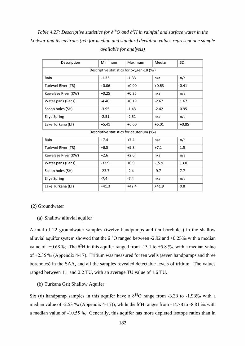
182

Table 4.27: Descriptive statistics for δ18O and δ2H in rainfall and surface water in the

Lodwar and its environs (n/a for median and standard deviation values represent one sample

available for analysis)

Description Minimum Maximum Median SD

Descriptive statistics for oxygen-18 (‰)

Rain -1.33 -1.33 n/a n/a

Turkwel River (TR) +0.06 +0.90 +0.63 0.41

Kawalase River (KW) +0.25 +0.25 n/a n/a

Water pans (Pans) -4.40 +0.19 -2.67 1.67

Scoop holes (SH) -3.95 -1.43 -2.42 0.95

Eliye Spring -2.51 -2.51 n/a n/a

Lake Turkana (LT) +5.41 +6.60 +6.01 +0.85

Descriptive statistics for deuterium (‰)

Rain +7.4 +7.4 n/a n/a

Turkwel River (TR) +6.5 +9.8 +7.1 1.5

Kawalase River (KW) +2.6 +2.6 n/a n/a

Water pans (Pans) -33.9 +0.9 -15.9 13.0

Scoop holes (SH) -23.7 -2.4 -9.7 7.7

Eliye Spring -7.4 -7.4 n/a n/a

Lake Turkana (LT) +41.3 +42.4 +41.9 0.8

(2) Groundwater

(a) Shallow alluvial aquifer

A total of 22 groundwater samples (twelve handpumps and ten boreholes) in the shallow

alluvial aquifer system showed that the δ18O ranged between -2.92 and +0.25‰ with a median

value of -+0.68 ‰. The δ2H in this aquifer ranged from -13.1 to +5.8 ‰, with a median value

of +2.35 ‰ (Appendix 4-17). Tritium was measured for ten wells (seven handpumps and three

boreholes) in the SAA, and all the samples revealed detectable levels of tritium. The values

ranged between 1.1 and 2.2 TU, with an average TU value of 1.6 TU.

(b) Turkana Grit Shallow Aquifer

Six (6) handpump samples in this aquifer have a δ18O range from -3.33 to -1.93‰ with a

median value of -2.53 ‰ (Appendix 4-17)), while the δ2H ranges from -14.78 to -8.81 ‰ with

a median value of -10.55 ‰. Generally, this aquifer has more depleted isotope ratios than in

183

the shallow alluvial aquifer. Tritium was <0.8 TU in all the four groundwater samples of the

Turkana Grit Shallow aquifer.

(c) Intermediate aquifer

A total of 20 groundwater samples from ten handpumps and ten boreholes were analysed for

oxygen-18 (18O) deuterium (2H) in the intermediate aquifer (Appendix 4-17). The δ18O ranged

from -3.92 to 0.07 ‰ with a median value of -2.55 ‰. The δ2H ranged between -11.30 to -4.54

‰ with a median value of -7.79 ‰. Groundwater samples of this aquifer adjacent to the

Turkwel River were more enriched in both 18O and 2H isotopes than those further away. Of

the 20 groundwater samples of the IA, tritium was determined on seven samples, where four

showed tritium values <0.8 TU. Tritium in the remaining three groundwater samples ranged

from 1.0 to 1.9 TU (Kakemera Church Hp = 1.0 TU, Chokochok Primary Hp = 1.9 TU, and

Napuu 4 Bh = 1.5 TU).

(d) Deep aquifer

The results of the isotope compositions for the samples of the deep aquifer are given in

Appendix 4-17). The δ18O for the Natirnalulung Bh (depth = 102) was +.23‰, and the δ2H was

+3.87‰. The δ18O of Napuu 1 (depth = 100) was -1.17‰ while the δ2H was +1.0‰. The

Natirnalulung borehole is more enriched in δ2H than in the δ18O counterpart, while the Napuu

1 Bh is more enriched in δ18O. Napuu 1 borehole has more depleted isotope ratios as compared

to that of the Natirnalulung Bh. The tritium for Natirnalulung Bh (Natir) was 2.1 TU, while

that of Napuu 1 was 1.0 TU.

(e) Depth unknown

Of the 44 boreholes and handpumps with unknown depth, the isotope compositions of oxygen-

18 and deuterium were determined for 41 samples (25 handpumps and 16 boreholes)

(Appendix 4-17). The δ18O ranged from -4.37 to -0.12 ‰ with a median value of -2.39 ‰. The

δ2H ranged between -24.7to +5.9 ‰ with a median value of -9.0 ‰. Generally, these samples

showed more δ2H as compared to the δ18O content. Tritium measurement for sixteen

groundwater samples (four boreholes and twelve handpumps) of wells with unknown depth

revealed values <0.8 TU for nine samples (four boreholes and five handpumps) and values

ranging between 1.2 and 1.8 TU for the rest seven handpumps samples.

184

Table 4.28: Descriptive statistics Results for oxygen-18, 2H and 3H groundwater samples in the

SAA, TGSA, IA, DA, and for wells with unknown depth (DU)

Description Minimum Maximum Median SD

Oxygen-18 (δ18O ‰)

SAA -2.92 0.25 -0.68 0.88

TGSA -3.33 -1.93 -2.53 0.50

IA -3.92 +0.07 -2.55 0.97

DA -1.17 -0.23 -0.70 0.66

DU -4.37 -0.12 -2.39 1.08

Deuterium (δ2H ‰)

SAA -13.1 +5.8 +2.3 5.4

TGSA -14.8 -8.8 -10.5 2.2

IA -11.3 +4.5 -7.8 4.4

DA -2.7 +3.9 +0.6 4.6

DU -24.7 +5.9 -9.0 6.3

Tritium (TU)

SAA 1.1 2.2 1.6 0.3

TGSA <0.8 n/a n/a n/a

IA 1.0 1.9 1.5 0.5

DA 1.0 2.1 1.6 0.8

DU 1.2 1.8 1.5 0.2

4.2.3.2 Isotopic ratios of oxygen-18 and deuterium

a) Selection of the linear regression model

The Global Mean Meteoric Water Line (GMWL) for three GNIP stations, Kericho, Soroti, and

Moyale, is given by equation δD = 8.0 18O + 10 (Craig, 1996). The significance and data source

for GMWL and LMWL is described in section 3.43. Regression statistics were tested to

determine the best regression model for the three GNIP stations (Figure 4.53). The LMWL for

Kericho GNIP station follows the equation δD = 7.7 x 18O + 12.2 with R2 = 0.90. The LMWL

for Soroti follows the equation δD = 8.5 x 18O + 13.8 with R2 = 0.99 while the LMWL for

Moyale GNIP station follows the equation 5.6947 x 18O + 8.3 with R2 = 0.98. These results

indicated that the Soroti GNIP station in Uganda, though not completely relating to the

observation data of the study area, was the best regression model for correlating with the

isotopic data. Soroti station also represents rainfall characteristics upstream of the study area,

185

that is, the Mt. Elgon region which is the source of the Turkwel river. It is also important to

note that the three regression lines for the GNIP stations intercepted at δ18O = -2.28 and δ2H =

-5.5, suggesting similar processes of isotope fractionation in the region.

Figure 4.53: Regression lines of δ2H versus δ18O for the nearby GNIP stations; Kericho,

Moyale and Soroti with their respective regression statistics

b) δ18O and δ2H ratio in rainfall and surface water

The isotopic compositions of the rainfall and surface water in Lodwar and its environs

displayed varied isotopic compositions (Figure 4.54). The rain sample of the Lodwar town

plotted above the LMWL, contrasting with the isotope composition of Turkwel River samples

that plotted below the meteoric water lines. One river sample of the flowing water of the

Kawalase River plotted below the LMWL, and slightly below that of the Turkwel River. The

scoop holes of the streams in the eastern section of Lodwar all plotted along the LMWL, while

those in the western part (Kawalase and Nakutan areas) plotted slightly below the meteoric

water line, indicating δ18O enrichment. All the water pan samples are below the LMWL while

Regression Statistics Kericho Soroti Moyale

Multiple R 0.9563 0.99751 0.991153

R Square 0.904902 0.995026 0.982384

Adjusted R Square 0.899308 0.994612 0.973575

Standard Error 6.64381 1.775293 3.714175

Observations 19 14 4

186

that of the Eliye spring is located on the meteoric water line. The Lake Turkana samples showed

enriched isotope ratios (δ18O and δ2H) relative to the local meteoric water line and relative to

all the types of water samples in the study area. By comparing the two lake samples, the one

collected on its shores at Eliye Spring (2461) is more enriched than that obtained at the Turkwel

delta (2462).

Figure 4.54: Relationship between δ18O and δ2H for the rain sample, Turkwel River,

Kawalase River, scoop holes, water pans and springs in the study area

c) δ18O and δ2H ratio in groundwater

The relationship between δ18O and δ2H was determined for groundwater samples of the SAA,

TGSA, IA, DA, and for the wells whose depth was unknown (Figure 4.55). The water samples

of the SAA plotted generally below the Soroti LMWL indicating δ18O enrichment relative to

the meteoric water (Figure 4.55a). The groundwater of the TGSA plotted along the LMWL

except for two samples (3394 and 3396) located at the contact zone of the Turkana grits and

the nepheline-phonolite at Lodwar town that exhibited δ18O enrichment and deviated from the

LMWL (Figure 4.55c). As compared to the SAA, the groundwater of the TGSA and showed

depleted δ18O and δ2H isotopes. The samples of the intermediate aquifer plotted around and

along the LMWL except for three samples (3341, 3374 and 3392) that were plotted in the SAA

field and two samples (3366 and 3368) that plotted above the meteoric water line, indicating

187

depleted δ18O ratio relative to that of the meteoric water. The δ2H/ δ18O plot of the wells with

unknown depth resulted in three distinct groups; group A that exhibited isotopic compositions

of the SAA; group B that plotted in the region of the IA, and group C that comprised only two

samples and plotted in the region of the TGSA (Figure 4.55d).

Figure 4.55: Regression analysis for δ18O and δ2H for SAA (<30m), IA (31-100m), and the

TGSA(<30m) in relation to the Soroti LMWL and the GMWL. The graph also shows the

position of the rain sample, Turkwel River samples, spring sample, samples of the DA

(>100), and the TGSA samples

4.2.3.3 Age of groundwater and recharge sources

a) Age of groundwater

Qualitative and quantitative techniques were used to determine the age of groundwater of the

Lodwar aquifers based on Clark and Fritz (1997, see section 3.4.3). The tritium values suggest

that the groundwater of the study area comprises recharge before the 1950s (< 0.8TU) and a

mixture of sub-modern and modern water (0.8 to 4.0 TU) (Clark and Fritz, 1997). The SAA,

IA and DA are characterised by sub-modern recharge (1.1 to 2.20 TU) with pockets of older

groundwater (<0.8) in the intermediate aquifer south-west of Lodwar town at Naotin, Nabuin

188

and Nachomin areas, and may extend further south-westwards. The TGSA primarily consists

of older (before the 1950s) groundwater with tritium <0.8 TU. Figure 4.57 shows the

distribution of tritium in the study area, showing relatively younger water located closer to the

Turkwel River. The tritium values ranged from 1.10 to 2.20 TU in the water samples of the

study area. Similar values have been observed by Sklash and Mwangi, (1991) in the north

eastern region of Kenya, including Marsabit county. Values between 0.17 to 1.82 TU have

been reported in Tanzania (McKenzie et al., 2001) and between 3.00 to 9.00 TU in Uganda

(Onugba and Aboh, 2009). Thus, although the East African waters are expected to have low

levels of tritium (< 1.0 TU), higher values can be recorded in various regions.

The age of groundwater was calculated using Equation 3.23 (section 3.4.3) for the water

samples with detectable levels of tritium – recharged after 1950. A detectable level of tritium

was found in 24 groundwater samples in the SAA, IA, DA and some of the DU wells. The

results revealed that recharge occurred for these samples between 2004 and 2018, indicating

about 0 to 14 years. Of the 24 groundwater samples used in age calculation, 16 samples showed

that they were recharged after 2010 (<10 years old) while the remaining eight are regarded to

be older (recharged between 2004 and 2009). Figure 4.56 shows the tritium trends in

groundwater of the LAAS (excluding the TGSA), indicating levels approaching pre-bomb

levels (1.0 TU) in 2018. No relationship was observed between tritium and depth of the wells

in the LAAS. See Appendix 4-18 for the specific ages of each of the 24 samples discussed

above.

189

Figure 4.56: Tritium trend in the groundwater of the LAAS between 2004 and 2018,

indicating 3H values approaching pre-bomb levels

0

0.5

1

1.5

2

2.5

2002 2004 2006 2008 2010 2012 2014 2016 2018 2020

Trit

ium

(TU

)

Year

190

Figure 4.57: Spatial distribution of tritium in groundwater in the Lodwar Alluvial Aquifer

System (LAAS); older groundwater is saline unless within the proximity of the Turkwel River

while the younger groundwater is fresh

b) Recharge sources

The Soroti LMWL has a slope and intercept (δD = 8.518O + 13.8), which is relatively higher

than that of the GMWL (δD = 818O + 10), indicating humid conditions (Taylor and Howard,

1996). The δ18O and δ2H isotopes of the rainfall in Lodwar plotted above the LMWL,

suggesting continental effects resulting in rainfall enriched in deuterium. The more enriched

values of oxygen-18 and deuterium in the Turkwel River over the local precipitation in Lodwar

town indicate rainfall characteristics in a highland catchment (H. Yeh et al., 2014). Evaporation

processes in the water pans, scoop holes, Turkwel and Kawalase Rivers resulted in depleted

isotope ratios (18O and 2H) relative to the LMWL. The Turkwel River originates south-east of

Lodwar town in the Mount Elgon region while the Kawalase River emanates from the western

191

part of Lodwar in the Loima Hills. Flow regulation and frequency of dam release, and

groundwater baseflows in the dry season may contribute to the depleted isotopic composition

of the Turkwel River relative to that of the precipitation. The scoop hole samples plotted along

the meteoric water lines, except for those in the Kawalase River, indicating isotopic

compositions of local rainfall.

The δ18O and δ2H isotopes in the groundwater of the SAA slightly deviated from that of the

local meteoric water line. Therefore, the groundwater of the SAA might be a mixture of

Turkwel River water and local rainfall, causing the effect of the river water recharge being

larger than that the infiltration of rainfall (Chen et al., 2019; Yeh et al., 2014). The spatial

distribution of δ18O and δ2H in groundwater samples (SAA, IA, DA, TGSA and DU) (Figure

4.58) shows enriched values of δ18O and δ2H closer to the Turkwel River and become depleted

away from the river channel. Water samples of the SAA and IA that plotted above the LMWL

are linked to direct recharge from local rainfall. These samples were few and sparsely

distributed within Nayuu and Lolupe areas of the study area. The analysis of the d-excess

indicates that the SAA has a relatively higher value (d =5.9), indicating its association with

recent rainfall recharge as compared to that of the IA (d = 2.5). The lower d-excess value of

the IA than that of the SAA suggests fractionation of oxygen and hydrogen isotopes along the

groundwater flow path from the shallow alluvial aquifer to the intermediate aquifer through

time (Taylor and Howard, 1996). The d-excess of the wells with unknown depth (d = 4.7)

slightly deviated from that of the SAA demonstrating that their majority in the shallow alluvial

aquifer, while the others are either in the IA and TGSA. The d-excess value of the TGSA (d-

excess = 0.2) represents that of groundwater associated with significant evaporation processes

(Levin et al., 2009). These findings indicate that the average recharge waters of this system are

significantly depleted compared to modern-day rainfall recharge waters (Acworth et al., 2014).

192

Figure 4.58: Spatial distribution of (a) δ18O and (b) δ2H for all the groundwater samples

showing isotope enrichment along the Turkwel River, suggesting diffuse recharge

Table 4.29: Regression results from the shallow alluvial aquifer (SAA), Turkana grits

shallow aquifer (TGSA), intermediate aquifer and for the wells with unknown depth (DU)

relative to the GMWL and LWML

Data Source Line Slope (a)

D-Excess (b)

MWL Equation (δD = a18O + b)

R2

GMWL 8 10 δD = 818O + 10 1

LMWL (Moyale) 5.7 8.3 δD = 5.718O + 8.3 0.98

Shallow alluvial aquifer 5.7 5.9 δD = 5.718O + 5.9 0.87

Turkana grit shallow aquifer 4.4 0.2 δD = 4.418O + 0.2 0.97

Intermediate aquifer 4.1 2.5 δD = 4.118O + 2.5 0.81

Depth Unknown (wells) 5.3 4.7 δD = 5.318O + 4.7 0.84

Development of Conceptual aquifer model

An aquifer conceptual model has been prepared based on information derived from a variety

of sources; (i) DEM profiles (ii) Borehole depth information of selected boreholes contained

in secondary data (iii) aquifer thickness derived from geophysics (ii) water type of each aquifer

based on Piper diagram, and (iii) surface geology and geological structures in the study area

obtained from geological mapping.

(a) Geological cross-sections

Four profiles were obtained from the digital terrain model of the study area to prepare

geological cross-sections (Figure 4.59);

193

(a) Line AB is oriented N-S and passes through the central part of Lodwar town. It traverses

the Precambrian Quartzo-feldspathic gneiss, Miocene nepheline-phonolite and, Cretaceous

Turkana grits. Holocene sediments are not exposed along line AB profile. From the secondary

data, the wells in this section are mainly in the SAA while the few in the IA are < 40 m deep.

(b) Line CD oriented N-S passes is 21 km located to the east of Lodwar town and through

Napuu area traversing the Cretaceous Turkana grits, Alluvial deposits on the Turkwel River,

Holocene sediments (both 4,000 and 10,000 Yr BP) on the southern part of the Turkwel River

that extends southwards into the Turkana grits. The secondary data indicated that the majority

of the boreholes in this section are in the intermediate aquifer and one borehole in the deep

aquifer (Napuu Bh).

(c) Line EF also running in an N-S trend passing through the nepheline-phonolite, Cretaceous

Turkana grits, a thin layer of alluvial sediments in the Turkwel River, Holocene sediments

(4,000 Yr BP) and again the Turkana grits south of the Turkwel River. Few wells have been

dug along this profile in the SAA within the Turkwel River, and the boreholes at the end of the

line (Nachomin area) are in the IA.

(d) Line GH is approximately 41 km running from the west to the east of the study area covering

areas with the majority of borehole and handpumps, indicating increased groundwater

abstraction. Cretaceous Turkana grits, Holocene sediments and Alluvial deposits describe the

surface geology along this line. The up-doming along this profile south of Lodwar town

represents underlying volcanic rocks. West of the profile line, the wells are situated in the SAA

and become deeper outwards of the Turkwel River into the IA. All the wells in the east of

Lodwar town along this profile are in the intermediate aquifer.

194

Figure 4.59: Cross-section lines (AB, CD, EF, and GH) representing differrent part of the

study area indicating variations in surface geology and topography

195

Figure 4.60: Geological cross-sections along for selected profiles in the study area, showing changes in the surface geology with depth

196

(b) Aquifer Conceptual model – Lodwar Alluvial Aquifer System

The Lodwar Alluvial Aquifer system comprises three sub-systems categorised based on depth as

follows; shallow alluvial aquifer (<30 m), intermediate aquifer (31-100 m), and the deep aquifer

(> 100) (cf. Olago 2018). The source of recharge to the aquifer is mainly through diffuse recharge

by the Turkwel River and from the surface water of the Kawalase River during the wet season.

Direct recharge from rainfall infiltration in the study area is expected to contribute aquifer recharge

during rainfall events. The conceptual model (Figure 4.61) outlines the shallow alluvial aquifer as

an unconfined system at depth < 30 m on either side of the Turkwel River. The intermediate and

the deep aquifer are both semi-confined with the highly permeable semi-confining layer.

Groundwater discharge mechanisms in the study area are mainly through groundwater abstraction

and evaporation.

197

Figure 4.61: Conceptual aquifer model of the Lodwar Alluvial Aquifer System showing the three

sub-systems; shallow alluvial aquifer (SAA), intermediate aquifer (IA) and deep aquifer (DA).

The SAA is unconfined while the IA and DA are semi-confined and are separed by semi-

impervious layers (aquitard)

198

4.3 Discussion

Lodwar Alluvial Aquifer System

Statistical and various geochemical methods were used to investigate the study area and to

analyze the datasets obtained from primary and secondary sources. .

4.3.1.1 Hydrogeological characteristics

(i) Surficial geology and the geological structures

The geology of the area is characterized by the four rock types (i) Basement system rocks – mainly

the quartzo-felspathic gneiss, (ii) sedimentary formations that comprise the Cretaceous Turkana

grits and sandstones, and the Quaternary to Holocene sediments, (iii) Paleogene and Neogene

volcanics that includes the augite basalts and the nepheline-phonolite and (iv) the alluvial deposits.

Geological mapping in Lodwar and its environs revealed that the groundwater sources have been

developed within the alluvial deposits and the Holocene sediments

Various factors such as physiography, climate, geology, and structural features such as lineaments

and dykes govern the occurrence and movement of groundwater (Senthilkumar et al., 2015).

Dykes are very common geological discontinuities recognised in occurrence of aquifers as altering

the flow of groundwater (Appleyard and Cook, 2009; Babiker and Gudmundsson, 2004; Comte et

al., 2017). Dolerite dykes were recorded in the Turkana grits and the quartzo-felspathic gneiss

following the NW-SE trending control the groundwater flow in the study area. Of interest in the

dolerite dyke in the Turkana grits within Lodwar town of about 1.5 m thickness and relatively

dense in nature than the surrounding grits. The dyke dissects the Lodwar alluvial aquifer system

into two major parts; the western part and the eastern section relative to the position of Lodwar

town in the study area. The groundwater sources developed near the dyke in the western section

of the LAAS are saline, suggesting limited flow of groundwater supporting mineral dissolution.

For much of the topography-driven groundwater flow, long and thick low-permeability dykes

serve as barriers (Babiker and Gudmundsson, 2004). The groundwater gathered by these dykes is

transported along their margins to the topographic depressions occupied fault zones of higher

permeability (Comte et al., 2017).

(ii) Petrography and rock geochemistry

The petrographic analysis and rock geochemistry of the rocks in the study area revealed that the

rock-forming minerals include pyroxenes, olivine, feldspars (plagioclase and orthoclase)

199

aluminosilicates, ferromagnesian minerals, amphiboles, quartz, micas and carbonates. As in all

arid areas physical and mechanical weathering is predominant.

Groundwater chemistry largely depends on the mineral composition of the rocks its flow paths

due to rock-water interactions (Lakshmanan and Kannan, 2007). Depending on the chemical

composition of the initial water, geological conditions, and time of residence, these chemical

reactions vary spatially and temporally. By hydrating the surface of minerals, hydrolyzing

minerals and replacing some of their exposed surface cations with hydrogen ions, and dissolving

minerals to remove mineral matter as solutes, water serves as a chemical weathering agent. Ferrous

iron is preferentially soluble in minerals, including ferromagnesian silicates, carbonates, and

magnetite (Enkin et al., 2020). This study found that Ca, Na, Fe, Mg, Al and K are the elements

that can be released to the groundwater through weathering of carbonates and silicates minerals

and oxidation reactions. Carbonate weathering, silicate weathering, halite and gypsum dissolution

and precipitation are common aquifer processes in arid areas (Lakshmanan and Kannan, 2007).

The compositions of trace elements on the other hand were generally low, indicating that they are

unlikely to be found in undesirable concentrations in groundwater.

(a) Carbonate weathering

Ca2+ and Mg2+ is realised to groundwater by dolomite (Equation 4-1) and calcite (Equation 4-2;

4-3) dissolution. The addition of HCO3- to groundwater is due to the dissolution of carbonates and

the reaction of silicates with carbonic acid (M. Kumar et al., 2006). ‘Kankar’ carbonates were

found in the Turkana grits, Holocene sediments and alluvial deposits within the study area,

suggesting they are the potential source of Ca2+ and HCO3-.

𝐶𝑎𝑀𝑔(𝐶𝑂3)𝑑𝑜𝑙𝑜𝑚𝑖𝑡𝑒 + 2𝐻2𝐶𝑂3 = 𝐶𝑎2+ + 𝑀𝑔2+ + 4𝐻𝐶𝑂3− (Equation 4-1)

𝐶𝑎𝐶𝑂3𝑐𝑎𝑙𝑐𝑖𝑙𝑡𝑒+ 𝐻2𝑆𝑂4 = 𝐶𝑎𝑆𝑂4 + 𝐻2𝑂 + 𝐶𝑂2 (Equation 4-2)

2𝐶𝑎𝐶𝑂3 𝑐𝑎𝑙𝑐𝑖𝑡𝑒 + 𝐻2𝐶𝑂3 = 2𝐶𝑎2+ + 2𝐻𝐶𝑂3−

(Equation 4-3)

200

(b) Silicate weathering

Silicate weathering involves hydrolysis reactions that use primary minerals and protons to form

silicate minerals (K, Ca, Fe and Mg) (Bhattacharya et al., 2008). All rocks in the study area are

rich in silica (SiO2 = >40 wt %), suggesting a high potential for silicate weathering and ion leaching

in aquifers. The presence of kaolinite in the Cretaceous Turkana grits suggests plagioclase feldspar

weathering involving albite (NaAlSi3O8). decomposition releasing Na+ and SiO2 to groundwater

(Equation 4-4). The increased K concentrations in the shallow alluvial aquifer and the intermediate

aquifer (Tanui et al., 2020) is linked to the high compositions of K2O (average =1.88 wt %) and

K (average = 0.35 wt %) in the Holocene sediments suggesting hydrolytic reaction in favour of

orthoclase feldspar (KAl3SiO8) (Equation 4-5) releasing K+ and soluble silica (H4SiO4).

Additional Ca2+ concentrations in groundwater is related to weathering of mineral anorthite

(CaAl2SiO8) (Equation 4-6). The occurrence of silicate weathering in the study area is subject to

spatial and temporal variations, dominating the Turkana grits and the Holocene sediments.

2𝑁𝑎𝐴𝑙𝑆𝑖3𝑂8 𝑎𝑙𝑏𝑖𝑡𝑒 + 2𝐻+ + 𝐻2𝑂 → 𝐴𝑙2𝑆𝑖2𝑂5(𝑂𝐻)4𝐾𝑎𝑜𝑙𝑖𝑛𝑖𝑡𝑒+ 2𝑁𝑎+ + 4𝑆𝑖𝑂2

(Equation 4-4)

2𝐾𝐴𝑙𝑆𝑖3𝑂8 𝑜𝑟𝑡ℎ𝑜𝑐𝑙𝑎𝑠𝑒 + 2𝐻+ + 9𝐻2𝑂 → 𝐴𝑙2𝑆𝑖2𝑂5(𝑂𝐻)4𝐾𝑎𝑜𝑙𝑖𝑛𝑖𝑡𝑒+ 2𝐾+ + 4𝐻4𝑆𝑖𝑂2

(Equation 4-5)

𝐶𝑎𝐴𝑙𝑆𝑖3𝑂8 𝑎𝑛𝑜𝑟𝑡ℎ𝑖𝑡𝑒 + 2𝐻+ + 𝐻2𝑂 → 𝐴𝑙2𝑆𝑖2𝑂5(𝑂𝐻)4𝐾𝑎𝑜𝑙𝑖𝑛𝑖𝑡𝑒 + 𝐶𝑎2+

(Equation 4-6)

Silicate weathering has been linked to higher concertation of Na+ in groundwater (M. Kumar et

al., 2006), a characteristic observed in the TGSA.

(iii) Sub-surface characteristics

The use of geophysics for subsurface investigations in groundwater studies has increased in the

recent years (Bello et al., 2017; Egai and Douglas, 2015; Kana et al., 2015). Vertical Electrical

sounding measurements utilizing Schlumberger array has also been applied by many researchers

201

(Bello et al., 2017; Egai and Douglas, 2015; Kana et al., 2013). The results of the resistivity

soundings in the LAAS revealed heterogenous sub-subsurface formations. Vertical and lateral

variations in the apparent resistivity values reflect changes in the geological units in the aquifer

(Bello et al., 2017). The modelled VES data revealed up to five geoelectric layers in the section A

of the LAAS, `three layers in section B and C and four within the Napuu (section D). In all the

four aquifer sections, the medium resistivities ranging between 20-65 Ohm- m were interpreted

an aquifer unit hosting fresh groundwater at varying depths between 15 to up to 130 m. In contrast,

the low resistivity values (< 10 Ohm-m) were associated with saline groundwater in the area as

determined by (Tanui et al., 2020). Saline groundwater in Lodwar and its environs are associated

with occurrence of Turkana grits and the Miocene volcanic rocks.

(iv) LAAS aquifer properties

The characteristics of the aquifers play a major role in the identification of potential groundwater

zones because they represent the rock structures through which the water flows (Kumar et al.,

2016). The hydrogeological conditions of the area were assessed based on the results of the pump

test records of boreholes previously drilled in the study area. Important aquifer characteristics such

as aquifer depth, transmissivity, yields, aquifer thickness and storage were determined.

The transmittivity of soil or rock is frequently determined by physical factors such as porosity,

particle size, and particle distribution and arrangement (Fabbri and Piccinini, 2013). The

transmittivity values reflect the variability in the thickness and permeability of the aquifer levels

(Kumar et al., 2016). Average transmissivity values indicate that the deep aquifer in Napuu has a

high groundwater potential (1316.11 m2/day), followed by the shallow aquifer (440.00 m2/day)

and then the intermediate aquifer (115.18 m2/day) (Kuria, 2013). The average optimum yields in

the shallow alluvial aquifer was 16.87 m3/h, 8.23 m3/h in the intermediate aquifer and 100.00 m3/h

in the DA within the Napuu area, reflecting the distribution of the transmissivity values. Optimum

yield is a unique aquifer parameter that can be used to establish a groundwater discharge and

management plan. It is closely related to subsurface lithology and other aquifer parameters (Fabbri

and Piccinini, 2013; Kumar et al., 2016). It helps control the depletion of the water level and

maintains a long-term stability in the aquifer. As far as groundwater is concerned, the aquifer

thickness is closely related to the transmission and storability of any soil (Shekhar, 2017). Based

on test pumping data obtained from the secondary sources and the geophysical measurements, the

thickness of the aquifer varied at each section of the aquifer; Section A (37 m), Section B (40 m),

Section C (30 m), and Section D (45 m). These values suggest that the high yields observed in the

202

Napuu area (section D) is associated with the prevailing aquifer thickness. The yields and the

aquifer thickness in the Turkana grits aquifer was not determined by this study due to unavailable

borehole logs and test pumping data. The Lodwar Alluvial Aquifer System covers 104.93 km2 of

land east and west of the Municipality of Lodwar with an estimated aquifer storage was 1.3 Billion

Cubic Meter (BCM), considered to be renewable in nature.

4.3.1.2 Hydrogeochemical characteristics

The evaluation of the water quality of the LAAS revealed that the system mainly hosts good

groundwater quality in wet and dry seasons except for except for a few wells, that included

LOWASCO Bh 2C. The water quality index was used to evaluate the seasonal changes in water

quality in the LAAS and in the TGSA. The TGSA revealed poor groundwater quality unfit for

human consumption in both seasons, therefore, it is not further discussed in terms of quality in the

next sections. The water quality index has widely been used to evaluate drinking water quality of

groundwater (Ansari and Hemke, 2013; Badmus et al., 2015; Heiß et al., 2020). Deteriorating

trends in water quality was observed in all the sub-systems of the LAAS during the wet season,

linked to mineral dissolution and flushing of contaminated recharge water into the aquifer by

recharge water. The contamination was due to high Fe2+ and Mn2+ ions in the shallow alluvial

aquifer linked to oxidizing conditions in the wet season (Yadav et al., 2020) while high F and EC

were the major factors affecting the water quality in the intermediate aquifer, suggesting

predominant mineral dissolution.

Shallow alluvial aquifers are known as highly pollution-prone (Muhammad et al., 2015; Yidana

et al., 2010a). In order to assess the anthropogenic effect on the quality of groundwater, nitrate

concentrations in groundwater samples were assessed. High levels of nitrate in drinking water are

undesirable due to the possible reduction in nitrite that may be hazardous to health, especially in

infants and pregnant women (Ramaroson et al., 2018). Furthermore, nitrate in groundwater is

primarily due to pollution, such as fertiliser or manure leaching, wastewater disposal, leakage from

septic tanks, etc., and thus suggests the potential presence of other harmful pollutants, such as

bacteria or pesticides (Guo et al., 2019; Lathamani et al., 2015). In arid urban areas, nitrate

contamination in shallow groundwater is linked to poor waste disposal and leaky sewerage

networks (Goni et al., 2019; Lapworth et al., 2017). Lodwar town lacks a functional sewerage

network (Hirpa et al., 2018; Olago, 2018), posing threat to the groundwater quality in the area

(Tanui et al., 2020). Increasing trends of nitrates were observed in the SAA and IA during the wet

season, an indication of potential aquifer pollution, with values approaching the water quality

203

guidelines within the town. Lapworth et al. (2017) determined that nitrate pollution is an

underlying issue in urban arid areas, always associated with poor sanitation and irrigation sources.

The water groundwater chemistry of the shallow alluvial aquifer during the wet season reflected

that of the river water indicating a high degree of connectivity. Similar findings have been

observed shallow alluvial aquifers in the sub-Saharan Africa (Walker et al., 2019). In addition,

evaluation of hydrochemical facies revealed that just as the Turkwel River, the shallow alluvial

aquifer was dominated by Ca-HCO3 water type. The calcium bicarbonate waters ae associated

with recent recharge (Walker et al.,2019). The Intermediate (samples from depths between 31-

100 m) and deep groundwater (samples from wells with depths >100 m) is of a NaHCO3 type

indicating higher mineralization due to longer residence times and greater distance of flow

(Walker et al., 2019). Pockets of Mg-HCO3 water were observed within the shallow alluvial and

intermediate aquifers. Aquifer chemistry in the SAA and IA is highly affected by seasonal

recharge pulses from the Turkwel flow, whereas direct rainfall recharge has a similar impact on

TGSA (Tanui et al., 2020). However, in the DA, there are no substantial variations in physico-

chemical parameters in the wet-dry season, indicating that recharge occurs over longer timescales

than the seasonal cycles for this aquifer. The Turkana grit shallow aquifer was Na-Cl water type

and became Na-HCO3 near the Holocene sediments, indicating substantial mineralization in the

grits due to mineral dissolution and evaporation processes. Minimal dilution of groundwater by

recharge water occurs in this aquifer near the Holocene sediments (Tanui et al., 2020).

This study compares with the findings of (Kumar et al., 2006) where the predominant

hydrochemical processes in an arid aquifer system were dissolution, weathering of carbonate and

silicate minerals, ion exchange, and surface water interaction.

4.3.1.3 Rainfall-surface water-groundwater interactions

The isotopes widely used in groundwater investigations are stable isotopes of the water molecule,

2H and 18O, and radioactive isotopes, tritium and carbon-14 (Sappa et al., 2012). This study utilized

2H, 18O and 3H isotopes to understand rainfall-surface water-groundwater interactions in Lodwar

and its environs. Mechanistic knowledge of the fundamental mechanisms for managing the spatial

patterns and temporal dynamics of groundwater-surface water interactions is essential to

maintaining drinking water supplies and ecological processes (Lewandowski et al., 2020). The

isotopic compositions of O and H in water, modified by meteoric processes, are useful tracers for

the determination of groundwater origin and movement, since they do not usually change as a

result of rock-water interactions (Clark and Fritz, 1997; Chen et al., 2018, 2019).

204

The groundwater recharge system in the alluvial plain consists of three complementary processes:

vertical rainfall infiltration, lateral infiltration through the fracture network and altered rocks, and

vertical drainage of the surface hydrographic network (Ramaroson et al., 2018). As compared to

the precipitation in Lodwar, the groundwater of the LAAS was isotopically depleted.

Consequently, precipitation may not be the primary mechanism for recharging the Lodwar

Alluvial Aquifer System. The proximity of the groundwater and river composition suggested that

the Turkwel river was a significant contributor to recharge in the SAA. Lateral infiltration of

groundwater from the SAA and the Turkwel River contributes recharge to the IA and the DA.

The EC values and the overall aquifer mineralization was observed to increase away from the

river (i.e. Turkwel river < SAA <IA <DA < TGSA) Tanui et al., 2020 where the EC value in the

Turkwel River is < 250 µS/cm and > 5000 µS/cm in the TGSA. Three recharge mechanisms are

identified to contribute recharge to the LAAS sub-systems; recharge of the SAA by the Turkwel

River related to mixing in the IA, recharge by Kawalase river in Napuu, Lolupe and Nayuu areas,

and direct rainfall recharge in few locations. This study also revealed that the groundwater of the

TGSA is not associated with modern rainfall.

Tritium is a radioactive hydrogen isotope. It has unique characteristics that make it distinctive

among the environmental tracers of groundwater pollution: it does not interfere with aquifer

materials when passing through porous media and is considered conservative geochemically

(Ramaroson et al., 2018). Qualitative and quantitative techniques were used to determine the age

of groundwater of the Lodwar aquifers based on Clark and Fritz (1997, see section 3.4.3) using

tritium. The tritium values in groundwater suggest that the groundwater of the study area

comprises recharge before the 1950s (< 0.8 TU) and a mixture of sub-modern and modern water

(0.8 to 4.0 TU) – post 1950s. The water samples with detectable levels of tritium in the SAA, IA

and DA (1.1 to 2.2) with more enriched values occurring closer to the Turkwel River.

Groundwater samples in the intermediate aquifer with no detectable levels of tritium were located

away from the river channel and had depths > 50 m, suggesting longer residence time as compared

to near the Turkwel River. Spatial distribution of tritium in the plain suggests a dynamic

mechanism for groundwater flow (Bayari et al., 2006), especially in the intermediate and deep

aquifers; some parts of intermediate aquifer had no measurable levels of tritium, while other parts

had values had values in range with that of the SAA. In addition, the tritium levels in the deep

aquifer were > 2.0, contradicting the average values of the intermediate aquifer. High and low

205

hydraulic conductivity units with rapid and slow groundwater velocity appear to exist side by side

in the aquifer (Bayari et al., 2006).

4.3.1.4 Development of Conceptual aquifer model

Rural communities in the sub-Saharan Africa utilize shallow aquifers for water supply. Increased

use of shallow groundwater can help to achieve multiple sustainable development goals (SDGs)

by having a positive effect on poverty, hunger and health (Walker et al., 2019). However, these

shallow aquifers are little studied and misunderstood, partially because of the lack of existing

hydrogeological evidence in many regions of sub-Saharan Africa (Walker et al., 2019; Xu et al.,

2019). Like many urban arid areas in the SSA, Lodwar town in Turkana county depends on

shallow aquifers (<30 m) to intermediate depth (31-100 m) (c.f. Olago 2018) for water supply.

The development of a hydrogeological conceptual model is crucial to a better understanding of

the hydrogeological system (Umar, 2006). Developing a conceptual model usually involves the

evaluation of existing topographic, geological and hydrometeorological data, which would

generally require, to varying degrees depending on the location of the study site, the addition of

new field investigations, laboratory analyses and additional monitoring (Walker et al., 2019). Due

to the complex distribution of lithological units in the plain, it is very difficult. A computational

model of a hydrogeological system is difficult to construct. Absence of this information limits the

use of numerical flow models that could be used to describe the aquifer's recharging process

(Bayari et al., 2006).

This study therefore developed a hydrogeological conceptual model for Lodwar Alluvial Aquifer

System, based on extensive field investigation of surface and sub-surface geology, geochemical

surveys, review of secondary data and investigation of surface-groundwater interaction in the

region. The secondary data and geophysics revealed that the depth of boreholes in the area range

between 5 to 110 m, reflecting groundwater abstraction in the shallow, intermediate and deep

aquifer systems. The hydrogeochemistry and water quality data suggested that fresh groundwater

is hosted in the alluvial deposits on the floodplains of the Turkwel River and in the adjacent

Holocene sediments (intermediate aquifer), suggesting interconnection between the two systems.

This evidence suggests that shallow groundwater flows laterally in directions that do not generally

coincide with surface water flow paths, as demonstrated by Walker (2019). Thus, recharging

deeper aquifers. The deep groundwater (> 100 m) was observed to mirror that of the IA within

the Napuu areas and that of the SAA at Natir, indicating possible hydrological gradients as in the

case of (Walker et al., 2019). This aquifer, therefore, determined that the sub-systems of the

206

LAAS; SAA, IA and the DA are separated from each other by a highly permeable aquiclude that

acts as a semi-confining layer. Besides, HCA demonstrates that there is some interaction between

the IA and the Napuu bh (Tanui et al., 2020). The oxygen and hydrogen isotopes revealed rainfall

associated with modern rainfall in most parts of the aquifer, especially within the SAA.

Implications for sustainable groundwater use, demand, and aquifer protection

The consequence of unsustainable use of groundwater is increasingly evident across many parts

of the world. Groundwater management is a serious problem that threatens groundwater

availability in many arid and semi-arid parts of the world. Cost-effective and easy to use methods

for augmenting groundwater resources in arid alluvial aquifers ensure sustainable management of

the water supply (Guo et al., 2019). Global water demand is highly influenced by population

expansion, urbanization, food, and energy security policies, as well as macroeconomic activities

such as trade globalization, changing diets, and increased consumption. According to the UN

(2015), the projected global water demand by 2050 is expected to increase by 55% related to

growing industrial and domestic water demands. Thus, competing demands make it difficult for

allocation decisions that will, in turn, threaten sustainable development. The investigation of the

LAAS presents a vulnerable system to both human activities (Tanui et al., 2020) and climate risks

(Hirpa et al., 2018).

The isotopic compositions of 18O and 2H in surface water and groundwater of the study area

provide evidence of recharge sources. The positive d-excess values in the Turkwel river (6.47)

and SAA (2.18) suggest that they are interlinked. The plots of the groundwater samples below the

LMWL indicate that the recharge water has undergone slight evaporation (Mckenzie et al., 2010;

Ochungo et al., 2019; Sklash and Mwangi, 1991). In addition, direct rainfall recharge also occurs

in the study area as indicated by the water samples above the LMWL. However, determining

isotopic compositions of more rainfall samples in the study area will help understand the isotopic

composition of rainfall in the region and generate a new local meteoric water line relevant to future

similar studies.

Water quality indices have been used by several studies as a tool for communicating complex

groundwater quality information (Dhanasekarapandian et al., 2016; Hamlat and Guidoum, 2018;

Kumar and James, 2013a). The WQI of the study area has indicated areas of good groundwater

quality for expansion of groundwater supplies and areas of poor groundwater quality to be

considered for piped network. Furthermore, the tritium results revealed that the SAA comprises

fully modern groundwater with 3H levels between 1.0 to 2.2 TU. The decreasing d-excess values

207

from the SAA (2.18) to the intermediate aquifer (-6.81) and TGSA (-8.14) indicate isotope

fractionation during the lateral groundwater flow (Bershaw et al., 2018). Thus, tritium-bearing

groundwater of the IA results from the dilution of originally tritium-free groundwater by a lateral

flow of diffuse river recharge through the alluvial aquifer (Hamutoko et al., 2017, 2018; Vu et al.,

2020). Therefore, conservation of the Turkwel River catchment is critical in the sustainability of

the LAAS. The long-term approaches need to incorporate evidenced-based groundwater

management policies that will address three key issues including (Guo et al., 2019); (i)

management of supply sources to improve water availability in time and space, (ii) management

of water demand needs including the efficiency of water use, sectoral interaction with economic

activities, and (iii) balancing of competing demands and preservation of the integrity of water-

dependent eco-system.

Chemical and isotopic analysis was used to characterize the groundwater of the study area. The

relatively depleted values of δ2H corresponds to the water chemistry in river water, where the

Kawalase river samples are slightly mineralised than in the Turkwel river (Fig 5). This is linked

to the prevailing climatic conditions of the rainfall source areas; Mt Elgon comprises a cool and

wet climate with relief rainfall Loima is hot and dry with convectional rainfall (Oiro et al., 2018;

Yusuf et al., 2018).

Aquifer mineralization is also observed to increases from the SAA, which is hydraulically

connected to the Turkwel River, to the intermediate aquifer in the Holocene sediments and into

the Turkana grits (Tanui et al., 2020). Thus, the most negative values of δ2H are associated with

highest EC values. The mixing of the Kawalase and Turkwel River water result in relatively

depleted δ18O and δ2H signatures in groundwater at Napuu-Lolupe areas. The more depleted

values of the δ18O and δ2H in the TGSA and lack of tritium in its waters is consistent with the

highly mineralised groundwater (Tanui et al., 2020), suggesting long groundwater residence time.

However, closer to the Holocene sediments, the groundwater in the Cretaceous Turkana grits

displays similar chemical and isotopic signatures with the tritium-free groundwater of the

intermediate, indicating that the tow systems are inter-connected. This evidence suggests that the

Turkwel river recharges the TGSA through lateral flow via subsurface channels and buried

geological structures (Sklash and Mwangi, 1991) in the Holocene sediments and the Turkana grits.

208

5 CHAPTER FIVE: CONCLUSIONS AND RECOMMENDATIONS

5.1 Conclusions

This study was conducted to determine and characterize the Lodwar Alluvial Aquifer System in

terms of its hydrogeological characteristics, water quality determination and to evaluate the natural

and anthropogenic factors influencing its groundwater chemistry, and to investigate its rainfall-

surface water-groundwater interaction regimes by use of stable environmental isotopes. The data

collected from hydrogeological, hydrogeochemistry and isotope studies were used to develop a

conceptual aquifer model, providing scientific evidence for sustainable, safe exploitation and

management. The conclusions drawn from each of the study objectives are presented below.

(a) Hydrogeological characteristics of the LAAS

Four distinct aquifer systems underlie Lodwar, and its environs are; three subsystems of the

Lodwar alluvial aquifer system (LAAS) (i) the shallow alluvial aquifer which is less than 30 m

deep with an average aquifer yield of 16.87 m3/h, (ii) the intermediate aquifer with depths ranging

from 31 to 100 m and average yield of 8.28 m3/h, and (iii) the deep aquifer with a depth greater

than 100 m and yields > 100 m3/h. The fourth aquifer system is in the Turkana grits with depth <

30 m and is characterised by highly saline and non-potable water. The shallow depths and good

aquifer yield of the LAAS present an opportunity to address the water security challenges in

Lodwar and its environs. The Lodwar Alluvial Aquifer System covers 104.93 km2 of land area. It

is aligned east-west, and Lodwar Municipality is in the central portion. Based on borehole drilling

and test pumping records and the geophysical measurements, the thickness of the aquifer varies

as follows; Section A (37 m), Section B (40 m), Section C (30 m), and Section D (45 m). The total

estimated aquifer storage is 1.3 Billion Cubic Meter (BCM). The transmissivities range from 21.60

to 116.64 m2/day. Within the Napuu region, high yielding boreholes can therefore be struck.

Water availability is directly linked to economic development and expansion of investment

opportunities. The evidence obtained from the study suggests that the LAAS is a strategic aquifer

with medium to high borehole yields and that it is cheap to exploit because of its shallow nature

(< 30 m to 110 m). Thus, the growth and expansion of Lodwar town depend on the sustainability

of the underlying aquifers (the LAAS). Therefore, the hydrogeological data collected and analysed

provides the basis for informed decisions during the development of new groundwater sources and

sustainable management of the Lodwar Alluvial Aquifer System and the process can apply to other

209

arid regions in Kenya. Furthermore, the study contributes the much needed scientific knowledge

for better understanding of ASAL alluvial aquifers in sub-Saharan Africa and other similar

regions worldwide.

(b) Aquifer hydrogeochemistry and vulnerability to pollution

The water quality index revealed that the LAAS has good drinking water quality during the dry

season. Although the water quality indices are within the drinking water quality during the wet

season, they deteriorate slightly relative to the dry season across all the sub-systems of the LAAS.

In the SAA during the wet season, high Fe2+ and Mn2+ are observed with Bh 2C, one of the

LOWASCO supply boreholes records high Mn2+ (0.5 mg/L). High fluoride concentrations

characterize the IA in the wet season. The water quality of the TGSA is not suitable for drinking

in all seasons due to its high alkalinity (pH > 8.50) and very high salinity with cation and anion

concentrations that are well in excess of drinking water guidelines. Generally, the LAAS presents

a vulnerable groundwater resource with regard to anthropogenic contamination, though currently,

anions that are used to track anthropogenic pollution, such as NO3, are still below the guideline

values for drinking water, elevated concentrations of NO3 occur in the groundwater within the

town region as compared to the groundwater in the rural sections of the LAAS. The lack of a

sewerage network and poor sanitation poses a threat to the water quality of the LAAS, particularly,

because the population of the town is rapidly growing hence potential point-source pollutant

sources such as on-site sanitation facilities are becoming more and more widespread.

The water quality index maps in groundwater quality studies are used by decision-makers to

identify areas of groundwater abstraction (good quality) and areas for piped water supply (poor

groundwater quality) as has been demonstrated for the LAAS. The lack of sewerage networks in

small towns in sub-Saharan Africa has contributed immensely to contamination of their shallow

aquifers. The evidence presented by the low NO3 levels in the LAAS indicates an opportunity to

protect the aquifer from potential human contamination risks.

(c) Rainfall-surface water-groundwater interactions

The environmental isotopes (oxygen and hydrogen) point to the Turkwel River as a vital recharge

source to the underlying shallow alluvial aquifer. The data confirm the existing linkage between

the Turkwel River and the Lodwar Alluvial Aquifer System as hypothesized by Olago (2018) and

Hirpa et al. (2018). Other recharge sources include direct infiltration of rainfall and flowing water

of the Kawalase River during the wet season that recharges the eastern areas of the LAAS,

210

including the Napuu area. Qualitative determination of the age of groundwater in the LAAS

indicates that recharge occurs in two regimes; (1) pre-1950 recharge consisting of non-detectable

tritium levels (< 0.8 TU) within some parts of the IA adjacent to the Turkana grits, and (2) recharge

after the 1950s with tritium levels ranging from 1.1 to 2.20 TU found in the Holocene sediments,

and with higher values recorded in close proximity to the Turkwel River. The young groundwater

occurs mainly in the SAA, vast parts of the IA and the DA, and was recharged between 2004 and

2018, with the SAA having the most recent recharge. The TGSA comprises older groundwater

recharged before the 1950s and this, in part, accounts for its highly mineralised groundwater

chemistry.

The existence of rainfall-surface water-groundwater interaction in the LAAS based on the close

association of the stable isotopes (18O, 2H and 3H) illustrates the aquifer's renewable nature by the

modern recharge. However, numerous studies have demonstrated that aquifers associated with the

recent rainfall (directly or indirectly) suffer vast impacts of climate variability, especially in arid

areas characterised by low rainfall usually < 250 mm. Thus, decision-makers require effective

interventions in terms of management, protection, and planning for informed and sustainable

aquifer use.

(d) Conceptual aquifer model

Comprehensive aquifer studies involving the development of accurate hydrogeological conceptual

models ensure sustainable development and use of groundwater. The conceptual aquifer model

was developed for the LAAS based on the data derived from the hydrogeological,

hydrogeochemistry and isotope studies. The conceptual model outlines the shallow alluvial aquifer

as an unconfined system at depth < 30 m on either side of the Turkwel River. The intermediate

and the deep aquifer are both semi-confined with a highly permeable semi-confining layer. The

aquifer obtains its recharge from rainfall (direct infiltration through the highly permeable sands)

and primarily through Turkwel River water infiltration (diffuse recharge). The hydrogeological

model provides essential information about the depth variation of each sub-system of the LAAS,

recharge mechanisms, and helps to predict the water quality within the aquifer sections. Generally,

it presents important hydrogeological and hydrogeochemical findings of the LAAS in a simplified

manner for informed groundwater development. The hydrogeological model obtained contributes

to the ongoing studies of the alluvial aquifers in the SSA that involve developing aquifer

conceptual models.

211

This study demonstrated that vigorous groundwater research involving the investigation of

hydrogeological properties of an aquifer, water quality and its hydrogeochemistry, as well as

understanding of recharge characteristics helps to provide evidence-based groundwater

management at local, regional and international levels. The study revealed important

hydrogeological characteristics of the LAAS such as the aquifer recharge, discharge mechanisms,

depth of the three aquifer sub-systems, and aquifer yields. Although the water quality results

indicated good drinking water quality for most wells in the LAAS, the rising trends of nitrates in

the shallow alluvial aquifer and the intermediate sub-system indicates their susceptibility to

anthropogenic contamination. The stable isotopes of oxygen-18, deuterium and tritium in

groundwater showed a close linkage with modern to sub-modern recharge, suggesting

vulnerability of the aquifers in Lodwar to climate variability. Overall, the study objectives were

achieved, but the lack of long-term groundwater times series in the study area limited utilization

of the water table fluctuation method to estimate the amount of recharge within the LAAS. This

reflects the importance of initiating groundwater monitoring across the sub-Saharan African

region to improve on evidence-informed sustainable management outcomes.

5.2 Recommendations

From the detailed findings presented by this study, the following recommendations are made:

(i) It is important to record accurate geologs during drilling and maintain these in a

database to improve on the understanding of the aquifer system, which will then

support more sustainable use and management models. This research was limited

to a greater extent by the lack of comprehensive data on borehole logging and test

pumping. The Water Resources Authority (WRA) should ensure ultimate compliance

by the drilling contractors on submission of full borehole completion reports for the

newly developed boreholes in the area.

(ii) There is a need for prudent water quality monitoring and management of

groundwater resources in Lodwar and its environs to ensure their sustainability

and safe use. Prior to this study, detailed water quality studies in the study area had

not been carried out, making it difficult to determine the past groundwater quality

status in the LAAS. However, this study indicated changes in water quality and aquifer

chemistry between the wet and the dry season. With the growing population and human

212

activities in the region, and the increasing variability of the climate, the aquifer's water

quality may be adversely affected. The datasets presented by this study provide a strong

basis for building a future sustainable water quality monitoring program by the WRA.

(iii) Urgent protection of the Lodwar Alluvial Aquifer System is critical to ensure the

elimination of potential contamination sources. Aquifer protection and sustainable use

– the water quality and aquifer geochemistry data indicated that the LAAS hosts good

drinking water quality and anthropogenic pollution effects are low. However, the lack of

a functional sewerage network in Lodwar municipality and poor sanitation distribution

continue to threaten the aquifer's future water quality. Improve sanitation in the area should

be improved as well as around the water points to minimize human pollution. The

evaluation of groundwater isotopes indicated aquifer recharge by the Turkwel River. Thus,

the suitability of the LAAS is dependent on the continuous existence of the Turkwel River,

suggesting the urgent need for catchment conservation and regulation of upstream

activities (within and outside the Turkana county). This calls for multi-stakeholder

approach and collaboration by all the parties involved. Within the study area, the LAAS

system boundary has been outlined based on the hydrogeological, hydrochemical and

isotope studies. Prevention of land encroachment in the aquifer will help minimize

pollution risks and the development of groundwater well-fields in the area. Aquifer

protection is also part of the Vision 2030 environmental protection goal. Furthermore,

there is need for accurate water quality index maps for other aquifers in the Turkana

County areas. The development of groundwater supply sources is capital intensive and

sometimes result in dry or saline water sources. The water quality index maps are easily

understood and will facilitate the determination of areas of good groundwater quality for

informed decisions regarding the groundwater development sites, especially in arid regions

where groundwater development challenges in terms of water quality are dominant.

(iv) The understanding of groundwater interaction regimes enhances understanding

of the recharge characteristics and quantification of recharge, enabling

groundwater resource managers to plan for sustainable supply and adopt

management options that consider the extent of climate variability being

experienced in their region. into the. Groundwater level monitoring of the Lodwar

Alluvial Aquifer System by the Turkana County Government and the Water Resources

213

Authority is required to allow for adequate and long-term data for the development of

the forward and inverse groundwater models. These models will be useful tools for

abstraction allocation in the area. More generally, such approaches will add to the very

few rainfall-surface water-groundwater interaction studies currently undertaken in

Sub-Saharan Africa.

5.3 Recommendations For Future Research

To further understand the extent of impacts of climate variability of the Lodwar aquifers and to

generate more information for decision making, future research areas include but not limited to;

- Climate variability continues to pose a threat to the sustainability of groundwater

resources globally. Its impacts on aquifers can be accurately measured using long-term

rainfall and groundwater time series. Groundwater level monitoring is non-existent in the

area. As part of the preparation for a future hydro-climatic study in the area, there is a need

to develop a groundwater monitoring program. The derived datasets will help a future

study quantify the extent of climate variability and assess the long-term impacts of climate

variability on the groundwater system. The Water Table Fluctuation (WTF) data will aid

in developing forward and inverse models for allocation of groundwater abstraction

accurate estimation of groundwater recharge.

- Geophysical models and lithostratigraphic logs can be used synergistically to improve

aquifer conceptual models. However, there was a lack of geological logs throughout the

study area and a lack of adequate rock outcrops to define the 3D lithostratigraphy of the

study area accurately. Although this study utilised geological mapping, hydrocensus,

geophysical measurements, water quality and isotope studies of rain samples, surface water

and groundwater to develop the aquifer conceptual model, a future study involving the use

of geological logs for boreholes in the study area will help to improve the current aquifer

model by application of numerical modelling.

- Seasonal measurements of groundwater isotopes help to estimate the amount of

recharge in an aquifer quantitatively. Due to this study's limited timelines, a future study

involving analysis of seasonal groundwater isotopes of oxygen-18, deuterium, and tritium

will help quantify the amount of recharge in the LAAS. Analysis of rainfall and surface

214

water samples in this research will help distinguish the amount of recharge attributed to

rainfall and that of surface water in the area, and accurately predict the impacts of climate

variability on recharge of the LAAS.

215

REFERENCES

Abdelshafy, M., Saber, M., Abdelhaleem, A., Abdelrazek, S. M., and Seleem, E. M. (2019).

Hydrogeochemical processes and evaluation of groundwater aquifer at Sohag city, Egypt.

Scientific African, 6, e00196. https://doi.org/10.1016/j.sciaf.2019.e00196

Abid, K., Zouari, K., Dulinski, M., Chkir, N., and Abidi, B. (2011). Hydrologic and geologic

factors controlling groundwater geochemistry in the Turonian aquifer (southern Tunisia).

Hydrogeology Journal, 19(2), 415–427. https://doi.org/10.1007/s10040-010-0668-z

Abiye, T., Masindi, K., Mengistu, H., and Demlie, M. (2018). Understanding the groundwater-

level fluctuations for better management of groundwater resource: A case in the

Johannesburg region. Groundwater for Sustainable Development, 7, 1–7.

https://doi.org/10.1016/j.gsd.2018.02.004

Aboubaker, M., Jalludin, M., and Razack, M. (2013). Hydrochemistry of a complex volcano-

sedimentary aquifer using major ions and environmental isotopes data: Dalha basalts

aquifer, southwest of Republic of Djibouti. Environmental Earth Sciences, 70(7), 3335–

3349. https://doi.org/10.1007/s12665-013-2398-8

Acharyya, S. K. (2002). Arsenic contamination in groundwater affecting major parts of southern

West Bengal and parts of western Chhattisgarh: Source and mobilization process. 82(6),

22–24.

Acworth, R. I., Rau, G. C., McCallum, A. M., Andersen, M. S., and Cuthbert, M. O. (2014).

Comprendre les systèmes connectés eaux de surface/eaux souterraines en utilisant

l’analyse de Fourier sur les variations de charge journalières et infra journalières.

Hydrogeology Journal, 23(1), 143–159. https://doi.org/10.1007/s10040-014-1182-5

Adelana, S., Fantong, W., Nedaw, D., and Duah, A. (2011). Groundwater and Health: Meeting

Unmet Needs in Sub-Saharan Africa. https://doi.org/10.1007/978-90-481-3426-7

Adimalla, N., Dhakate, R., Kasarla, A., and Taloor, A. K. (2020). Appraisal of groundwater quality

for drinking and irrigation purposes in Central Telangana, India. Groundwater for

Sustainable Development, 10, 100334. https://doi.org/10.1016/j.gsd.2020.100334

216

Adomako, D., Maloszewski, P., Stumpp, C., Osae, S., Akiti, T. T., Adomako, D., Maloszewski,

P., Stumpp, C., Osae, S., and Akiti, T. T. (2010). Estimating groundwater recharge from

water isotope ( δ H , δ O ) depth profiles in the Densu River basin , Ghana Estimating

groundwater recharge from water isotope ( δ 2 H , δ 18 O ) depth. Hydrological Sciences

Journal – Journal Des Sciences Hydrologiques, 8(55), 2150–3435.

https://doi.org/10.1080/02626667.2010.527847

Afzali, A., Shahedi, K., Habib, M., Roshan, N., Solaimani, K., and Vahabzadeh, G. (2015).

Groundwater Quality Assessment in Haraz Alluvial Fan, Iran Full Length Research Paper

Groundwater Quality Assessment in Haraz Alluvial Fan , Iran. October 2014.

https://doi.org/10.12983/ijsres-2014-p0346-0360

Aggarwal, P. K., and Froehlich, K. (2016). ENVIRONMENTAL ISOTOPS IN

GROUNDWATER STUDIES. Groundwater, II.

Aghazadeh, N., Chitsazan, M., and Golestan, Y. (2017). Hydrochemistry and quality assessment

of groundwater in the Ardabil area, Iran. Applied Water Science, 7(7), 3599–3616.

https://doi.org/10.1007/s13201-016-0498-9

Águila, J. F., Samper, J., and Pisani, B. (2019). Parametric and numerical analysis of the estimation

of groundwater recharge from water-table fluctuations in heterogeneous unconfined

aquifers. Hydrogeology Journal, 27(4), 1309–1328. https://doi.org/10.1007/s10040-018-

1908-x

Agyemang, P. C. O., Roberts, E. M., Downie, B., and Sertich, J. J. W. (2019). Sedimentary

provenance and maximum depositional age analysis of the Cretaceous? Lapur and

Muruanachok sandstones (Turkana Grits), Turkana Basin, Kenya. Geological Magazine,

156(8), 1334–1356. https://doi.org/10.1017/S0016756818000663

Ahmed, M., Talukder, M., Mojid, M. A., and Samad, M. (1998). A study of hydrogeological

characteristics and properties of Muktagacha aquifer. Bangladesh Journal of Agricultural

Engineering, 9, 11–16.

Alam, K., and Ahmad, N. (2014). Determination of aquifer geometry through geophysical

methods: A case study from Quetta Valley, Pakistan. Acta Geophysica, 62(1), 142–163.

https://doi.org/10.2478/s11600-013-0171-8

217

Alhawdar, Z. (2014). Method Development for the Analysis of Aluminum, Calcium, Magnesium

and Iron in Sedimentary Rocks Recommended Citation. Pittsburg State University.

Allison, G. B., and Hughes, M. W. (1978). The use of environmental chloride and tritium to

estimate total recharge to an unconfined aquifer. Soil Research, 16(2), 181–195.

https://doi.org/10.1071/sr9780181

Al-Ruwaih, F. M. (2017). Hydrogeology and Groundwater Geochemistry of the Clastic Aquifer

and Its Assessment for Irrigation, Southwest Kuwait. In Aquifers—Matrix and Fluids.

InTech. https://doi.org/10.5772/intechopen.71577

Al-Shaibani, A. M. (2008). Hydrogeology and hydrochemistry of a shallow alluvial aquifer,

western Saudi Arabia. Hydrogeology Journal, 16(1), 155–165.

https://doi.org/10.1007/s10040-007-0220-y

Anderson, M. P., and Woessner, W. W. (1992). Applied groundwater modeling: Simulation of

flow and advective transport. Academic Press.

https://books.google.co.ke/books/about/Applied_Groundwater_Modeling.html?id=vVIne

qegO4QCandredir_esc=y

Andrés-Doménech, García-Bartual, R., Montanari, A., and Marco, J. B. (2015). Climate and

hydrological variability: The catchment filtering role. Hydrol. Earth Syst. Sci, 19, 379–

387. https://doi.org/10.5194/hess-19-379-2015

Ansari, J. A., and Umar, R. (2019). Evaluation of hydrogeochemical characteristics and

groundwater quality in the quaternary aquifers of Unnao District, Uttar Pradesh, India.

HydroResearch, 1, 36–47. https://doi.org/10.1016/J.HYDRES.2019.01.001

Ansari, K., and Hemke, N. M. (2013). Water Quality Index for Assessment of Water Samples Of

Different Zones In Chandrapur City. 3(3), 233–237.

APHA, A. P. H. A. (1995). Standard Methods for the Examination of Water and Wastewater Part

1000 Standard Methods for the Examination of Water and Wastewater.

https://www.mwa.co.th/download/file_upload/SMWW_1000-3000.pdf

Appleyard, S., and Cook, T. (2009). Reassessing the management of groundwater use from sandy

aquifers: Acidification and base cation depletion exacerbated by drought and groundwater

218

withdrawal on the Gnangara Mound, Western Australia. Hydrogeology Journal, 17(3),

579–588. https://doi.org/10.1007/s10040-008-0410-2

Arambourg, C. (1933). Mammifères Miocènes du Turkana (Afrique Orientale). Masson et Cie.

Arambourg, C., and Wolff, R. (1969). Nouvelles Donnees Paleontologiques Sur L’age Des ‘Gres

Du Lubur’ (Turkana Grits) A L’ouest Du Lac Rodolphe.

Ashley, G. M., Mworia, J. M. A., Muasya, A. M., Owen, R. B., and Driese, S. G. (2004).

Sedimentation and recent history of a freshwater wetland in a semi-arid environment:

Loboi Swamp, Kenya, East Africa. 1–21. https://doi.org/10.1111/j.1365-

3091.2004.00671.x

Ashraf, M. A. M., Yusoh, R., Sazalil, M. A., and Abidin, M. H. Z. (2018). Aquifer

Characterization and Groundwater Potential Evaluation in Sedimentary Rock Formation.

Journal of Physics: Conference Series, 995, 012106. https://doi.org/10.1088/1742-

6596/995/1/012106

Atuahene, B. (2017). Interaction of Surface Water and Groundwater in the Nile River Basin and

Peizometric Evidence. We Want What’s Ours: Learning from South Africa’s Land

Restitution Program, 18. https://doi.org/10.1590/S1516-18462008000300012

Avery, S. T. (2013). What future for Lake Turkana? African Studies Centre, 1–56.

Avery, S. T., and Tebbs, E. J. (2018). Lake Turkana, major Omo River developments, associated

hydrological cycle change and consequent lake physical and ecological change. Journal of

Great Lakes Research, 44(6), 1164–1182. https://doi.org/10.1016/j.jglr.2018.08.014

Ayenew, T. (2008). The distribution and hydrogeological controls of fluoride in the groundwater

of central Ethiopian rift and adjacent highlands. 1313–1324.

https://doi.org/10.1007/s00254-007-0914-4

Baalousha, H. (2011). Fundamentals of Groundwater Modelling (pp. 113–130).

Babiker, M., and Gudmundsson, A. (2004). The effects of dykes and faults on groundwater flow

in an arid land: The Red Sea Hills, Sudan. Journal of Hydrology, 297(1), 256–273.

https://doi.org/10.1016/j.jhydrol.2004.04.018

219

Badmus, B. S., Ozebo, V. C., Idowu, O. A., Ganiyu, S. A., and Olurin, O. T. (2015). Seasonal

variations of physico chemical properties and quality index of groundwater of hand-dug

wells around Ajakanga Dump Site in Southwestern Nigeria. Research Journal of Physics,

9(1), 1–10. https://doi.org/10.3923/rjp.2015.1.10

Bai, L., Wang, Y., Zhou, Y., Liu, L., Yan, Z., and Li, F. (2016). Research on the process-based

risk evaluation method of groundwater pollution for contaminated site. Water Science and

Technology: Water Supply, 16(1), 150–162. https://doi.org/10.2166/ws.2015.118

Barilari, A., Quiroz Londoño, M., Paris, M. del C., Lima, M. L., and Massone, H. E. (2020).

Groundwater contamination from point sources. A hazard index to protect water supply

wells in intermediate cities. Groundwater for Sustainable Development, 10, 100363.

https://doi.org/10.1016/j.gsd.2020.100363

Batelaan, O., and Smedt, F. D. E. (2001). WetSpass: A flexible, GIS based, distributed recharge

methodology for regional groundwater modelling. 269, 11–17.

Bates, B., Kundzewicz, Z. W., and IPCC (Eds.). (2008). Climate change and water.

Bayari, S., Ozyurt, N. N., Hatipoglu, Z., and Kilani, S. (2006). Groundwater age: A vital

information in protecting the groundwater dependent ecosystem. In A. Baba, K. W. F.

Howard, and O. Gunduz (Eds.), Groundwater and Ecosystems (pp. 33–46). Springer

Netherlands. https://doi.org/10.1007/1-4020-4738-X_3

Bekesi, G., and Mcconchie, J. (1998). Regional Groundwater Recharge Modelling Using the

Monte-Carlo Technique in the Manawatu Region, New Zealand. 1–18.

Bello, R., Emujakporue, G. O., Mkpese, U. U., and Gladman, B. G. (2017). The use of Vertical

Electrical Sounding (VES) to investigate the extent of groundwater contamination and

lithology delineation at a dumpsite in Aluu Community, Rivers State. Scientia Africana,

16(1), Article 1. https://doi.org/10.4314/sa.v16i1.

Belt, C. J. (1964). Atomic Absorption Spectrophotometry. Journal of Economic Geology, 59, 240–

258.

Bershaw, J., Bershaw, and John. (2018). Controls on Deuterium Excess across Asia. Geosciences,

8(7), 257. https://doi.org/10.3390/geosciences8070257

220

Bhattacharya, P., Ramanathan, A. L., Mukherjee, A. B., Bundschuh, J., Chandrasekharam, D., and

Keshari, A. K. (2008). Groundwater for Sustainable Development: Problems, Perspectives

and Challenges. CRC Press.

Birkle, P., Torres Rodríguez, V., and González Partida, E. (1998). The water balance for the Basin

of the Valley of Mexico and implications for future water consumption. Hydrogeology

Journal, 6(4), 500–517. https://doi.org/10.1007/s100400050171

Boah, D. K., Twum, S. B., and Pelig-ba, K. B. (2015). Mathematical Computation of Water

Quality Index of Vea Dam in Upper East Region of Ghana. Environmental Sciences, 3(1),

11–16. https://doi.org/10.12988/es.2015.4116

Boulton, S., and Whittaker, A. (2009). Quantifying the slip rates, spatial distribution and evolution

of active normal faults from geomorphic analysis: Field examples from an oblique-

extensional Graben, Southern Turkey. Geomorphology, 104, 299–316.

https://doi.org/10.1016/j.geomorph.2008.09.007

Brassington, and Younger. (2010). A proposed framework for hydrogeological conceptual

modelling. Water and Environment Journal, 24(4), 261–273.

https://doi.org/10.1111/j.1747-6593.2009.00173.x

Brears, E., and Post, R. (2014). NVCA Water Table Fluctuation Study. 1(Figure 1), 1–17.

Brindha, K., Rajesh, R., Murugan, R., and Elango, L. (2011). Fluoride contamination in

groundwater in parts of Nalgonda District, Andhra Pradesh, India. Environmental

Monitoring and Assessment, 172(1–4), 481–492. https://doi.org/10.1007/s10661-010-

1348-0

Bruthans, J., Kůrková, I., and Kadlecová, R. (2019). Factors controlling nitrate concentration in

space and time in wells distributed along an aquifer/river interface (Káraný, Czechia).

Hydrogeology Journal, 27(1), 195–210. https://doi.org/10.1007/s10040-018-1854-7

Burnham, C. (2019). (PDF) A Study of UAV Photogrammetry Software. ResearchGate.

https://www.researchgate.net/publication/335749992_A_Study_of_UAV_Photogrammet

ry_Software

221

Butler, L. R. P., and Kokot, M. L. (1971a). ATOMIC ABSORPTION. In National Physical

Research Laboratory (pp. 205–206).

Research Laboratory (pp. 205–206).

Calvache, M. L., Duque, C., Gomez Fontalva, J. M., and Crespo, F. (2011). Processes affecting

groundwater temperature patterns in a coastal aquifer. International Journal of

Environmental Science and Technology, 8(2), 223–236.

https://doi.org/10.1007/BF03326211

Carter, J. F., and Barwick, V. J. (2011). Good Practice Guide for Isotope Ratio Mass Spectrometry

FIRMS. http://www.forensic-isotopes.org/assets/IRMS Guide Finalv3.1_Web.pdf

Casanova, J., Devau, N., and Pettenati, M. (2016). Managed Aquifer Recharge: An Overview of

Issues and Options. In A. J. Jakeman, O. Barreteau, R. J. Hunt, J.-D. Rinaudo, and A. Ross

(Eds.), Integrated Groundwater Management (pp. 413–434). Springer International

Publishing. https://doi.org/10.1007/978-3-319-23576-9_16

Chacha, R. (2014). Method for analysing soil samples for mineral composition using XRD (pp. 1–

12).

Chae, G.-T., Kim, K., Yun, S.-T., Kim, K.-H., Kim, S.-O., Choi, B.-Y., Kim, H.-S., and Rhee, C.

W. (2004). Hydrogeochemistry of alluvial groundwaters in an agricultural area: An

implication for groundwater contamination susceptibility. Chemosphere, 55(3), 369–378.

https://doi.org/10.1016/J.CHEMOSPHERE.2003.11.001

Chen, X., Wang, G., and Wang, F. (2019). Classification of Stable Isotopes and Identification of

Water Replenishment in the Naqu River Basin, Qinghai-Tibet Plateau. Water, 11(1), 46.

https://doi.org/10.3390/w11010046

Chen, Z., Grasby, S. E., and Osadetz, K. G. (2004). Relation between climate variability and

groundwater levels in the upper carbonate aquifer , southern Manitoba , Canada. 290,

43–62. https://doi.org/10.1016/j.jhydrol.2003.11.029

Chenini, I., Farhat, B., and Ben Mammou, A. B. (2010). Identification of major sources controlling

groundwater chemistry from a multilayered aquifer system. Chemical Speciation and

Bioavailability, 22(3), 183–189. https://doi.org/10.3184/095422910X12829228276711

222

Chilton, J., Dahi, E., Lennon, M., and Jackson, P. (2006). Fluoride in Drinking-water.

Chilton, J., and Seiler, K.-P. (2006). Groundwater occurrence and hydrogeological environments.

In Protecting Groundwater for Health. Managing the Quality of Drinking-water Sources.

IWA Publishing,. http://www.bvsde.paho.org/bvsacd/cd59/protecting/sect1-2.pdf

Clark, I. D. (Ian D., and Fritz, P. (Peter). (1997). Environmental isotopes in hydrogeology. CRC

Press/Lewis Publishers. https://www.crcpress.com/Environmental-Isotopes-in-

Hydrogeology/Clark-Fritz/p/book/9781566702492

Cloutier, V., Lefebvre, R., Savard, M. M., Bourque, É., and Therrien, R. (2006).

Hydrogeochemistry and groundwater origin of the Basses-Laurentides sedimentary rock

aquifer system, St. Lawrence Lowlands, Québec, Canada. Hydrogeology Journal, 14(4),

573–590. https://doi.org/10.1007/s10040-005-0002-3

Cobbing, J. (2020). Groundwater and the discourse of shortage in Sub-Saharan Africa.

Hydrogeology Journal, 28(4), 1143–1154. https://doi.org/10.1007/s10040-020-02147-5

Coetsiers, M., Kilonzo, F., and Walraevens, K. (2009). Hydrochemistry and source of high

fluoride in groundwater of the Nairobi area , Kenya. 53(December 2008).

Comte, J. C., Cassidy, R., Obando, J., Robins, N., Ibrahim, K., Melchioly, S., Mjemah, I., Shauri,

H., Bourhane, A., Mohamed, I., Noe, C., Mwega, B., Makokha, M., Join, J. L., Banton,

O., and Davies, J. (2016). Challenges in groundwater resource management in coastal

aquifers of East Africa: Investigations and lessons learnt in the Comoros Islands, Kenya

and Tanzania. Journal of Hydrology: Regional Studies, 5, 179–199.

https://doi.org/10.1016/j.ejrh.2015.12.065

Comte, J.-C., Wilson, C., Ofterdinger, U., and González‐Quirós, A. (2017). Effect of volcanic

dykes on coastal groundwater flow and saltwater intrusion: A field-scale multiphysics

approach and parameter evaluation. Water Resources Research, 53(3), 2171–2198.

https://doi.org/10.1002/2016WR019480

Craig, H. (1961). Isotopic Variations in Meteoric Waters. Science, 133(3465), 1702.

https://doi.org/10.1126/science.133.3465.1702

223

Dandar, O., Okamoto, A., Uno, M., Batsaikhan, U., Ulziiburen, B., and Noriyoshi, T. (2018).

Drone brings new advance of geological mapping in Mongolia: Opportunities and

challenges. Mongolian Geoscientist, 53–57. https://doi.org/10.5564/mgs.v0i47.1063

Dash, S., Borah, S. S., and Kalamdhad, A. (2018). Monitoring and assessment of Deepor Beel

water quality using multivariate statistical tools. Water Practice and Technology, 13(4),

893–908. https://doi.org/10.2166/wpt.2018.098

Dennehy, K. F., Reilly, T. E., and Cunningham, W. L. (2015). Disponibilité des eaux souterraines

aux Etats-Unis d’Amérique: La valeur des évaluations quantitatives régionales.

Hydrogeology Journal, 23(8), 1629–1632. https://doi.org/10.1007/s10040-015-1307-5

Dhanasekarapandian, M., Chandran, S., Devi, D. S., and Kumar, V. (2016). Spatial and temporal

variation of groundwater quality and its suitability for irrigation and drinking purpose

using GIS and WQI in an urban fringe. Journal of African Earth Sciences, 124, 270–288.

https://doi.org/10.1016/j.jafrearsci.2016.08.015

Dhungel, R., and Fiedler, F. (2016). Water Balance to Recharge Calculation: Implications for

Watershed Management Using Systems Dynamics Approach. Hydrology, 3(1), 13.

https://doi.org/10.3390/hydrology3010013

Dodson, R. G. (Ministry of N. R. (1971). Geology the Area Area South of Lodwar. 87.

Douglas, K. S. O. R. K. (2015). Evaluation of major factors influencing the geochemistry of

groundwater using graphical and multivariate statistical methods in Yenagoa city ,

Southern Nigeria. Applied Water Science, 27–37. https://doi.org/10.1007/s13201-014-

0166-x

Doust, H., and Sumner, H. S. (2007). Petroleum systems in rift basins – a collective approach

inSoutheast Asian basins. Petroleum Geoscience, 13(2), 127–144.

https://doi.org/10.1144/1354-079307-746

Ducrocq, S., Boisserie, J.-R., Tiercelin, J.-J., Delmer, C., Garcia, G., Kyalo, M. F., Leakey, M. G.,

Marivaux, L., Otero, O., Peigné, S., Tassy, P., and Lihoreau, F. (2010). New Oligocene

vertebrate localities from Northern Kenya (Turkana basin). Journal of Vertebrate

Paleontology, 30(1), 293–299. https://doi.org/10.1080/02724630903413065

224

Edmunds, W. M., and Smedley, P. L. (2013). Fluoride in Natural Waters. In Fluoride in Natural

Waters. https://doi.org/10.1007/978-94-007-4375-5

Egai, A. O., and Douglas, R. K. (2015). Aspects of Geophysical Survey Using Vertical Electrical

Sounding (VES) for Groundwater Exploration in Parts of Ahoada West LGA of Rivers

State, Southern Nigeria. Geosciences, 5(1), 31–38.

Egan, P., and Price, M. (2014). Our Global Water Towers: Ensuring Ecosystem Services From

Mountains Under Climate Change – A Policy Brief (UNESCO).

Elango, L., and Kannan, R. (2007). Chapter 11 Rock–water interaction and its control on chemical

composition of groundwater. In Developments in Environmental Science (Vol. 5, pp. 229–

243). Elsevier. https://doi.org/10.1016/S1474-8177(07)05011-5

Engelen, V. V. (1984). Kenya Soil Survey: An Assessment of the Irrigation Suitability of the Soils

of The Nakwamoru Area (Turkana District) (pp. 1–25). Ministry of Agriculture - National

Agricultural Laboratory. https://edepot.wur.nl/480078

Enkin, R. J., Hamilton, T. S., and Morris, W. A. (2020). The Henkel Petrophysical Plot:

Mineralogy and Lithology from Physical Properties. Geochemistry, Geophysics,

Geosystems, 21(1), e2019GC008818. https://doi.org/10.1029/2019GC008818

Fabbri, P., and Piccinini, L. (2013). Assessing transmissivity from specific capacity in an alluvial

aquifer in the middle Venetian plain (NE Italy). Water Science and Technology, 67(9),

2000–2008. https://doi.org/10.2166/wst.2013.074

Falkenmark, M. (2019). Rapid Population Growth and Water Scarcity: The Predicament of

Tomorrow’ s Africa. Population and Development Review, 16(1990), 81–94.

Famiglietti, J. S. (2014). The global groundwater crisis. Nature Climate Change, 4(11), 945–948.

https://doi.org/10.1038/nclimate2425

FAO. (2018). Southern Africa Resilience Strategy 2018–2021 (p. 36). Food Africultural

Organization (FAO).

Faye, S. C., Diongue, M. L., Pouye, A., Gaye, C. B., Travi, Y., Wohnlich, S., Faye, S., and Taylor,

R. G. (2019). Tracing natural groundwater recharge to the Thiaroye aquifer of Dakar,

225

Senegal. Hydrogeology Journal, 27(3), 1067–1080. https://doi.org/10.1007/s10040-018-

01923-8

Feibel, C. S. (2011). A Geological History of the Turkana Basin. Evolutionary Anthropology,

20(6), 206–216. https://doi.org/10.1002/evan.20331

Foster, S. S. D., and Chilton, P. J. (2003). Groundwater: The processes and global significance of

aquifer degradation. Philosophical Transactions of the Royal Society B: Biological

Sciences, 358(1440), 1957–1972. https://doi.org/10.1098/rstb.2003.1380

Foster, S., Tuinhof, A., and Steenbergen, F. V. (2012). Managed groundwater development for

water-supply security in Sub-Saharan Africa: Investment priorities. 38(3), 359–366.

Garba Abdullahi, M., Nasiru Usman, U., Ekhwan Toriman, M., Juahir, H., Auwalu Rabiu, A., and

Isiyaka, H. (2014). Assessment of Groundwater Quality Using Multivariate Statistical

Techniques in Terengganu Groundwater Pattern Recognition Based on Rainfall

Distribution in Terengganu Malaysia View project Effect of Light Pollution View project

Assessment of Groundwater Quality Using Multivariate Statistical Techniques in

Terengganu. Science and Technology, 4(3), 42–49.

https://doi.org/10.5923/j.scit.20140403.02

Gardner, K. K., and Vogel, R. M. (2005). Predicting Ground Water Nitrate Concentration from

Land Use. 43(3), 343–352.

Garrels, R. M., and Berner, R. A. (1983). The Global Carbonate-Silicate Sedimentary System—

Some Feedback Relations. In P. Westbroek and E. W. de Jong (Eds.), Biomineralization

and Biological Metal Accumulation: Biological and Geological Perspectives Papers

presented at the Fourth International Symposium on Biomineralization, Renesse, The

Netherlands, June 2–5, 1982 (pp. 73–87). Springer Netherlands.

https://doi.org/10.1007/978-94-009-7944-4_6

Gates, J. B., Edmunds, W. M., Ma, J., and Sheppard, P. R. (2008). A 700-year history of

groundwater recharge in the drylands of NW China. Holocene, 18(7), 1045–1054.

https://doi.org/10.1177/0959683608095575

226

Gaye, C. B., and Edmunds, W. M. (1996). Groundwater recharge estimation using chloride, stable

isotopes and tritium profiles in the sands of northwestern Senegal. Environmental Geology,

27(3), 246–251. https://doi.org/10.1007/BF00770438

Geological map of Kenya (MERD). (1987).

Ghaffar, A., Tariq, T., Mashiatullah, A., and Ali, S. M. (2017). Hydrological and environment

tritium investigation to evaluate groundwater in capital territory of Pakistan. Water Science

and Technology: Water Supply, 17(2), 433–451. https://doi.org/10.2166/ws.2016.149

Ghoraba, S. M., and Khan, A. D. (2013). Hydrochemistry and groundwater quality assessment in

Balochistan province, Pakistan. International Journal of Research and Reviews in Applied

Sciences, 17(2), 185–199.

Giménez-Forcada, E. (2010a). Dynamic of Seawater Interface using Hydrochemical Facies

Evolution Diagram (HFE-D). https://doi.org/10.1111/j.1745-6584.2009.00649.x

Gleeson, T., Allen, D. M., and Ferguson, G. (2012). Teaching hydrogeology: A review of current

practice. 2159–2168. https://doi.org/10.5194/hess-16-2159-2012

Glover, E. T., Akiti, T. T., and Osae, S. (2012a). Geoscience Major ion chemistry and

identification of hydrogeochemical processes of groundwater in the Accra Plains.

Geoscience, 50, 10279–10288.

Glover, E. T., Akiti, T. T., and Osae, S. (2012b). Geoscience Major ion chemistry and

identification of hydrogeochemical processes of groundwater in the Accra Plains.

Geoscience, 50, 10279–10288.

Goni, I. B., Sheriff, B. M., Kolo, A. M., and Ibrahim, M. B. (2019). Assessment of nitrate

concentrations in the shallow groundwater aquifer of Maiduguri and environs,

Northeastern Nigeria. Scientific African, 4, e00089.

https://doi.org/10.1016/j.sciaf.2019.e00089

González-Trinidad, J., Pacheco-Guerrero, A., Júnez-Ferreira, H., Bautista-Capetillo, C., and

Hernández-Antonio, A. (2017). Identifying groundwater recharge sites through

environmental stable isotopes in an alluvial aquifer. Water (Switzerland), 9(8), 1–12.

https://doi.org/10.3390/w9080569

227

Goudarzi, S., Jozi, S. A., Monavari, S. M., Karbasi, A., and Hasani, A. H. (2017). Assessment of

groundwater vulnerability to nitrate pollution caused by agricultural practices. Water

Quality Research Journal of Canada, 52(1), 64–77.

https://doi.org/10.2166/wqrjc.2017.031

Green, T. R. (2016). Linking Climate Change and Groundwater. In A. J. Jakeman, O. Barreteau,

R. J. Hunt, J.-D. Rinaudo, and A. Ross (Eds.), Integrated Groundwater Management (pp.

97–141). Springer International Publishing. https://doi.org/10.1007/978-3-319-23576-9_5

Grundmann, G., and Scholz, H. (2015). Preparation methods in Mineralogy and Geology: The

preparation of thin sections, polished sections, acetate foil prints, preparation for

elutriation analysis and staining tests for the optical and electron microscopy.

Guo, Q., Zhou, Z., Huang, G., and Dou, Z. (2019). Variations of groundwater quality in the multi-

layered aquifer system near the Luanhe river, China. Sustainability (Switzerland), 11(4).

https://doi.org/10.3390/su11040994

Haile-Meskale, M. (2017). An Overview of Saturation State of Groundwater with Respect to Some

Common Minerals in South Central Ontario. International Journal of Sciences: Basic and

Applied Research (IJSBAR), Volume 36(5), 32–47.

Hamlat, A., and Guidoum, A. (2018). Assessment of groundwater quality in a semiarid region of

Northwestern Algeria using water quality index (WQI). Applied Water Science, 8(8), 1–

13. https://doi.org/10.1007/s13201-018-0863-y

Hamutoko, J. T., Wanke, H., Beyer, M., Gaj, M., and Koeniger, P. (2018). Spatio-temporal

variations of hydrochemical and isotopic patterns of groundwater in hand-dug wells: The

Cuvelai-Etosha Basin, Namibia. Proceedings of the International Association of

Hydrological Sciences, 378, 29–35. https://doi.org/10.5194/piahs-378-29-2018

Hamutoko, J. T., Wanke, H., Koeniger, P., Beyer, M., and Gaj, M. (2017). Hydrogeochemical and

isotope study of perched aquifers in the Cuvelai-Etosha Basin, Namibia. Isotopes in

Environmental and Health Studies, 53(4), 382–399.

https://doi.org/10.1080/10256016.2016.1273913

228

Hawkins, S. (2016). Using a drone and photogrammetry software to create orthomosaic images

and 3D models of aircraft accident sites. 26.

Healy, R. W. (2010). Estimating Groundwater Recharge. Cambridge University Press.

Heiß, L., Bouchaou, L., Tadoumant, S., and Reichert, B. (2020). Index-based groundwater

vulnerability and water quality assessment in the arid region of Tata city (Morocco).

Groundwater for Sustainable Development, 10, 100344.

https://doi.org/10.1016/j.gsd.2020.100344

Hemker, K., and Bakker, M. (2005). Calibration and Reliability in Groundwater Modelling: From

Uncertainty to Decision Making (Proceedings of ModelCARE’ Complex groundwater

whirl systems (Vol. 304). IAHS Publ. https://iahs.info/uploads/dms/13505.50-281-287-

IAHS304-07-181.pdf

Henkes, G. A., Moreira, M. C., Yang, D., and Thomas, E. (2018). A modern isotope hydrology of

the Turkana Basin. 2018, PP31B-1654.

Hinkle, B. S. R., and Survey, U. S. G. (1997). Quality of Shallow Ground Water in Alluvial

Aquifers of the Willamette Basin, Oregon,.

Hinzman, L. D., Wegner, M., and Lilly, M. R. (2000). Hydrologic Investigations of groundwater

and surface-water interactions in subarctic Alaska. Nordic Hydrology, 31(4–5), 339–356.

https://doi.org/10.2166/nh.2000.0020

Hirpa, F. A., Dyer, E., Hope, R., Olago, D. O., and Dadson, S. J. (2018). Journal of Hydrology:

Regional Studies Finding sustainable water futures in data-sparse regions under climate

change: Insights from the Turkwel River basin, Kenya. Journal of Hydrology: Regional

Studies, 19(August), 124–135. https://doi.org/10.1016/j.ejrh.2018.08.005

Hove, A. R. T., and Ongweny, G. S. O. (1974). AN OUTLINE OF KENYA’S GROUNDWATER

QUALITY. Journal of Eastern African Research and Development, 4(1), 67–97.

Hughes, M. (1933). Notes on the Geological Succession, Tectonics, and Economic Geology of the

Western Half of Kenya Colony. 3.

229

Irvine, T. N., and Baragar, W. R. A. (1971). A Guide to the Chemical Classification of the

Common Volcanic Rocks. Canadian Journal of Earth Sciences, 8(5), 523–548.

https://doi.org/10.1139/e71-055

Islam, Md. M., Lenz, O. K., Azad, A. K., Ara, M. H., Rahman, M., Hassan, N., Islam, Md. M.,

Lenz, O. K., Azad, A. K., Ara, M. H., Rahman, M., and Hassan, N. (2017). Assessment of

Spatio-Temporal Variations in Water Quality of Shailmari River, Khulna (Bangladesh)

Using Multivariate Statistical Techniques. Journal of Geoscience and Environment

Protection, 05(01), 1–26. https://doi.org/10.4236/gep.2017.51001

Jang, W., Engel, B., Harbor, J., and Theller, L. (2017). Aquifer Vulnerability Assessment for

Sustainable Groundwater Management Using DRASTIC. Water, 9(10), 792.

https://doi.org/10.3390/w9100792

Jaroslav, V., and Van der Gun, J. (2004). The world’s groundwater resources (p. Report Nr IP

2004-1). International Groundwater Resources Assessment Centre (IGRAC).

http://geocompendium.grid.unep.ch/index.htm

Jassas, H., and Merkel, B. (2014). Estimating groundwater recharge in the semiarid Al-Khazir:

Gomal basin, north Iraq. Water (Switzerland), 6(8), 2467–2481.

https://doi.org/10.3390/w6082467

JICA. (2012). Water Potential Study in Turkana County (pp. 231–256).

Jimenez, B., and Chávez, A. (2004). Quality assessment of an aquifer recharged with wastewater

for its potential use as drinking source: “El Mezquital Valley” case. Water Science and

Technology, 50(2), 269–276. https://doi.org/10.2166/wst.2004.0141

Joshi, S. K., Rai, S. P., Sinha, R., Gupta, S., Densmore, A. L., Rawat, Y. S., and Shekhar, S.

(2018). Tracing groundwater recharge sources in the northwestern Indian alluvial aquifer

using water isotopes (δ18O, δ2H and 3H). Journal of Hydrology, 559, 835–847.

https://doi.org/10.1016/j.jhydrol.2018.02.056

Kana, J. D., Djongyang, N., Dadjé, A., and Raїdandi, D. (2013). Vertical Electrical Soundings for

Subsurface Layers and Groundwater Investigations in the Mayo Kani Area in Cameroon.

International Journal of Science and Research (IJSR), 396–401.

230

Kanda, I., and Suwai, J. (2013). Hydrogeochemistry of Shallow and Deep Water Aquifers of

Menengai Geothermal Area, Kenya Rift Valley. 37, 8.

Karegi, S., Macharia, K., Muthengia, W., and Mwiti, M. (2018). Hydrogeochemistry of Ground

Water in Mbeere South Sub-County, Kenya. International Journal of Chemistry, 10, 173.

https://doi.org/10.5539/ijc.v10n4p173

Kaufmann, G. (2009). Modelling karst geomorphology on different time scales. Geomorphology,

106(1), 62–77. https://doi.org/10.1016/j.geomorph.2008.09.016

Kebede, S. (2005). Groundwater recharge, circulation and geochemical evolution in the source

region of the Blue Nile River , Ethiopia. Applied Geochemistry, 20(2005), 1658–1676.

https://doi.org/10.1016/j.apgeochem.2005.04.016

Kebede, S., Travi, Y., and Asrat, A. (2008). Groundwater origin and flow along selected transects

in Ethiopian rift volcanic aquifers. 55–73. https://doi.org/10.1007/s10040-007-0210-0

Kebede, S., Travi, Y., and Stadler, S. (2010a). Groundwaters of the Central Ethiopian Rift:

Diagnostic trends in trace elements, δ18O and major elements. Environmental Earth

Sciences, 61(8), 1641–1655. https://doi.org/10.1007/s12665-010-0479-5

Kebede, S., Travi, Y., and Stadler, S. (2010b). Groundwaters of the Central Ethiopian Rift:

Diagnostic trends in trace elements, δ18O and major elements. Environmental Earth

Sciences, 61(8), 1641–1655. https://doi.org/10.1007/s12665-010-0479-5

Kendall, C., and Holland, H. D. (2003). Stable Isotope Applications in Hydrologic Studies. In H.

D. Holland and K. K. Turekian (Eds.), Treatise on Geochemistry (pp. 319–364).

Pergamon. https://doi.org/10.1016/B0-08-043751-6/05081-7

Khatri, N., and Tyagi, S. (2014). Influences of natural and anthropogenic factors on surface and

groundwater quality in rural and urban areas. Frontiers in Life Science, 8(1), 23–39.

https://doi.org/10.1080/21553769.2014.933716

KNBS. (2009). The 2009 Kenya Population and Housing Census (Cencus Report VOLUME IC;

Counting Our People for the Implementation of Vision 2030”, pp. 1–546). Kenya National

Bureau of Statistics. https://s3-eu-west-

1.amazonaws.com/s3.sourceafrica.net/documents/21195/Census-2009.pdf

231

KNBS. (2019). Kenya Population and Housing Census (Population By County and Subcounty

Volume 1; pp. 1–49). Kenya National Bureau of Statistics.

http://housingfinanceafrica.org/app/uploads/VOLUME-I-KPHC-2019.pdf

Koskei, E. C., Kitetu, J. J., and Recha, C. W. (2018). Analysis of spatial variability in rainfall

trends in Baringo County, Kenya. 12(September), 296–304.

https://doi.org/10.5897/AJEST2016.2214

Kotchoni, D. O. V., Vouillamoz, J. M., Lawson, F. M. A., Adjomayi, P., Boukari, M., and Taylor,

R. G. (2018). Relationships between rainfall and groundwater recharge in seasonally

humid Benin: A comparative analysis of long-term hydrographs in sedimentary and

crystalline aquifers. Hydrogeology Journal, 1–11. https://doi.org/10.1007/s10040-018-

1806-2

Kumar, Balasubramanian, A., Kumar, R. S., Dushiyanthan, C., Thiruneelakandan, B., Suresh, R.,

Karthikeyan, K., and Davidraju, D. (2016). Assessment of groundwater potential based on

aquifer properties of hard rock terrain in the Chittar–Uppodai watershed, Tamil Nadu,

India. Applied Water Science, 6(2), 179–186. https://doi.org/10.1007/s13201-014-0216-4

Kumar, M., Ramanathan, AL., Rao, M. S., and Kumar, B. (2006). Identification and evaluation of

hydrogeochemical processes in the groundwater environment of Delhi, India.

Environmental Geology, 50(7), 1025–1039. https://doi.org/10.1007/s00254-006-0275-4

Kumar, P. (2013a). Interpretation of groundwater chemistry using piper and chadhas diagrams: A

comparative study from perambalur taluk. Elixirpublishers.Com, 54, 12208–12211.

Kumar, P. (2013b). Interpretation of groundwater chemistry using piper and chadhas diagrams: A

comparative study from perambalur taluk. Elixirpublishers.Com, 54, 12208–12211.

Kumar, P. J. S., and James, E. J. (2013a). Development of Water Quality Index (WQI) model for

the groundwater in Tirupur district, South India. Chinese Journal of Geochemistry, 32(3),

261–268. https://doi.org/10.1007/s11631-013-0631-5

Kumar, P. J. S., and James, E. J. (2013b). Development of Water Quality Index (WQI) model for

the groundwater in Tirupur district, South India. Chinese Journal of Geochemistry, 32(3),

261–268. https://doi.org/10.1007/s11631-013-0631-5

232

Kumar, S., Thirumalaivasan, D., and Radhakrishnan, N. (2014). GIS Based Assessment of

Groundwater Vulnerability Using Drastic Model. Arabian Journal for Science and

Engineering, 39(1), 207–216. https://doi.org/10.1007/s13369-013-0843-3

Kumari, B., Mondal, M. R., Tiwary, R., and Srivastava, K. K. (2014). Physico-chemical

characterization and water quality index of ground water of Dhanbad town area. Advances

in Applied Science Research, 5(3), 286–292.

Kundzewicz, Z. W., Mata, L. J., Arnell, N. W., Doll, P., Jimenez, B., Miller, K., Oki, T., Sen, Z.,

and Shiklomanov, I. (2008). The implications of projected climate change for freshwater

resources and their management. Hydrological Sciences Journal, 1(53), 2–10.

https://doi.org/10.1623/hysj.53.1.3

Kuria, Z. (2011). Kenya: A Natural Outlook: Groundwater Distribution and Aquifer

Characteristics in Kenya. In Kenya: A Natural Outlook: Geo-Environmental Resources

and Hazards (1st ed., Vol. 16, pp. 83–105). Elsevier B.V.

Kuria, Z. (2013). Chapter 8—Groundwater Distribution and Aquifer Characteristics in Kenya. In

P. Paron, D. O. Olago, and C. T. Omuto (Eds.), Developments in Earth Surface Processes

(Vol. 16, pp. 83–107). Elsevier. https://doi.org/10.1016/B978-0-444-59559-1.00008-6

Kurniawan, A. (2009). BASIC IP2 WIN TUTORIAL. 32.

Kuroda, K., and Fukushi, T. (2008). Groundwater Contamination in Urban Areas. In S. Takizawa

(Ed.), Groundwater Management in Asian Cities: Technology and Policy for Sustainability

(pp. 125–149). Springer Japan. https://doi.org/10.1007/978-4-431-78399-2_7

Lakshmanan, E., and Kannan, R. (2007). Chapter 11 Rock–water interaction and its control on

chemical composition of groundwater. Developments in Environmental Science, 5.

https://doi.org/10.1016/S1474-8177(07)05011-5

Lapworth, D. J., Nkhuwa, D. C. W., Okotto-Okotto, J., Pedley, S., Stuart, M. E., Tijani, M. N.,

and Wright, J. (2017). Urban groundwater quality in sub-Saharan Africa: Current status

and implications for water security and public healthQualité des eaux souterraines urbaines

en Afrique sub-saharienne: État actuel et implications pour la sécurité de

233

l’approvisionnement en e. Hydrogeology Journal, 25(4), 1093–1116.

https://doi.org/10.1007/s10040-016-1516-6

Lathamani, R., Janardhana, M. R., Mahalingam, B., and Suresha, S. (2015a). Evaluation of

Aquifer Vulnerability Using Drastic Model and GIS: A Case Study of Mysore City,

Karnataka, India. Aquatic Procedia, 4(Icwrcoe), 1031–1038.

https://doi.org/10.1016/j.aqpro.2015.02.130

Lautze, J., Holmatov, B., Saruchera, D., and Villholth, K. G. (2018). Conjunctive management of

surface and groundwater in transboundary watercourses: A first assessment. Water Policy,

20(1), 1–20. https://doi.org/10.2166/wp.2018.033

Lee, C. H., Chen, W. P., and Lee, R. H. (2006). Estimation of groundwater recharge using water

balance coupled with base-flow-record estimation and stable-base-flow analysis.

Environmental Geology, 51(1), 73–82. https://doi.org/10.1007/s00254-006-0305-2

Lerner, D. N., Issar, A. S., and Simmers, I. (1990). Groundwater recharge: A guide to

understanding and estimating natural recharge.

Levin, N. E., Zipser, E. J., and Cerling, T. E. (2009). Isotopic composition of waters from Ethiopia

and Kenya: Insights into moisture sources for eastern Africa. Journal of Geophysical

Research (Atmospheres), 114, D23306. https://doi.org/10.1029/2009JD012166

Lewandowski, J., Meinikmann, K., and Krause, S. (2020). Groundwater–Surface Water

Interactions: Recent Advances and Interdisciplinary Challenges. Water, 12(1), 296.

https://doi.org/10.3390/w12010296

Li, B. D., Zhang, X. H., Xu, C. Y., Zhang, H., and Song, J. X. (2015). Water balance between

surfacewater and groundwater in the withdrawal process: A case study of the Osceola

watershed. Hydrology Research, 46(6), 943–953. https://doi.org/10.2166/nh.2015.137

Li, X., Wu, H., Qian, H., and Gao, Y. (2018). Groundwater chemistry regulated by hydrochemical

processes and geological structures: A case study in Tongchuan, China. Water

(Switzerland), 10(3). https://doi.org/10.3390/w10030338

Liu, C., Chia, Y., Chuang, P., Chiu, Y., and Tseng, T. (2018). Impacts of hydrogeological

characteristics on groundwater-level changes induced by earthquakes. 451–465.

234

Lokhande, P. B., and Mujawar, H. A. (2016a). Graphic Interpretation and Assessment of Water

Quality in the Savitri River Basin. International Journal of Scientific and Engineering

Research, 7(3), 1113–1123.

Lokhande, P. B., and Mujawar, H. A. (2016b). Graphic Interpretation and Assessment of Water

Quality in the Savitri River Basin. International Journal of Scientific and Engineering

Research, 7(3), 1113–1123.

MacDonald, A. M., Bonsor, H. C., Dochartaigh, B. É. Ó., and Taylor, R. G. (2012). Quantitative

maps of groundwater resources in Africa. Environmental Research Letters, 7(2), 024009.

https://doi.org/10.1088/1748-9326/7/2/024009

Macdonald, A. M., Davies, J., Nations, U., Programme, E., Olorunfemi, F., Rilwanu, T. Y., Inkani,

A. I., Olasehinde, P. I., Journal, K., Abdul, Solomon, S., Nwankwoala, H. O., Danert, K.,

Gesti Canuto, J., British Geological Survey, Nanbakhsh, H., Tasi ’, O, I. E., Mallam I, …

Decision, M. (2016). Surface Water and Groundwater Resources Assessment In Wajir

County For Decision Making Final Report Water Resources Management Authority in

Collaboration with the State Department For Devolution. Journal of Environment and

Earth Science, 1(May), 1–17. https://doi.org/10.13140/RG.2.2.21914.64964

MacDonald, and Adelana, S. (2008). Groundwater research issues in Africa. In S. Adelana and

MacDonald (Eds.), Applied Groundwater Studies in Africa (Vol. 20086152). Taylor

andamp; Francis. https://doi.org/10.1201/9780203889497.ch1

MacDonald, and Davies, J. (2000). A brief review of groundwater for rural water supply in sub-

Saharan Africa (Tecnhical Report WC/00/33; Overseas Geology Series, p. 30). British

Geological Survey.

Maina, J. W., and Gaciri, S. J. (2010). Contributions to the hydrogeochemistry of the area to the

immediate north of Nairobi Conservation Area, Kenya. Journal of African Earth Sciences

(1983), 2(3), 227–232. https://doi.org/10.1016/S0731-7247(84)80017-8

Makokha, M. (2019). Groundwater Quality Analyses along Kenyan Coastal Region, Case Study

of Kilifi County. International Journal of Environment and Geoinformatics, 6, 1–14.

https://doi.org/10.30897/ijegeo.466933

235

Malvić, T., Velić, J., and Peh, Z. (2005). Geologia Croatica Qualitative – Quantitative Analyses

of the Influence of Depth and Lithological Composition on Lower Pontian Sandstone

Porosity in the Central Part of Bjelovar Sag ( Croatia ). 73–86.

Martínez, D. E., and Bocanegra, E. M. (2002). Hydrogeochemistry and cation-exchange processes

in the coastal aquifer of Mar Del Plata, Argentina. Hydrogeology Journal, 10(3), 393–408.

https://doi.org/10.1007/s10040-002-0195-7

Mason, P., and Gibson, A. B. (1957). GEOLOGY OF THE KALOSSIA-TIATI AREA: DEGREE

SHEET 26, N.E. AND S.E. QUARTERS. Geological Survey of Kenya.

Maurice, L., Taylor, R. G., Tindimugaya, C., Macdonald, A. M., Johnson, P., Kaponda, A., Owor,

M., and Sanga, H. (2018). Characteristics of high-intensity groundwater abstractions from

weathered crystalline bedrock aquifers in East Africa. https://doi.org/10.1007/s10040-

018-1836-9

Mbithi, F. M., Kariuki, P. C., and Gikuma-Njuru, P. (2017). Assessment of the Impact of

Groundwater Fluoride on Human Health: A Case Study of Makindu District in Kenya.

Mckenzie, J. M., Mark, B. G., Thompson, L. G., Schotterer, U., and Lin, P.-N. (2010). A

hydrogeochemical survey of Kilimanjaro (Tanzania): Implications for water sources and

ages. Hydrogeology Journal, 18(4), 985–995. https://doi.org/10.1007/s10040-009-0558-4

McKenzie, J. M., Siegel, D. I., Patterson, W., and McKenzie, D. J. (2001). A geochemical survey

of spring water from the main Ethiopian rift valley, southern Ethiopia: Implications for

well-head protection. Hydrogeology Journal, 9(3), 265–272.

https://doi.org/10.1007/s100400100134

Meng, F., Xiao, C., Liang, X., Wang, G., and Sun, Y. (2019). Regularity and a statistical model

of surface water and groundwater interaction in the Taoer River alluvial fan, China. Water

Supply, 1–12. https://doi.org/10.2166/ws.2019.118

Miljević, N., Boreli-Zdravković, D., Obradović, V., Golobočanin, D., and Mayer, B. (2012).

Evaluation of the origin of nitrate influencing the Ključ groundwater source, Serbia. Water

Science and Technology, 66(3), 472–478. https://doi.org/10.2166/wst.2012.179

236

Mook, W. G. (2000). Environmental isotopes in the hydrological cycle. Volume I.pdf. Technical

Documents in Hydrology, 1(39), 1–291.

Moore, J. E. (2011). Field Hydrogeology: A Guide for Site Investigations and Report Preparation,

Second Edition. CRC Press.

Morán-Ramírez, J., Ledesma-Ruiz, R., Mahlknecht, J., and Ramos-Leal, J. A. (2016). Rock–water

interactions and pollution processes in the volcanic aquifer system of Guadalajara, Mexico,

using inverse geochemical modeling. Applied Geochemistry, 68, 79–94.

https://doi.org/10.1016/J.APGEOCHEM.2016.03.008

Moridi, A., Tabatabaie, M. R. M., and Esmaeelzade, S. (2018). Holistic Approach to Sustainable

Groundwater Management in Semi-arid Regions. International Journal of Environmental

Research, 12(3), 347–355. https://doi.org/10.1007/s41742-018-0080-4

Mostafa, M. G., Uddin, S. M. H., and Haque, A. B. M. H. (2017). Assessment of hydro-

geochemistry and groundwater quality of Rajshahi City in Bangladesh. Applied Water

Science, 7(8), 4663–4671. https://doi.org/10.1007/s13201-017-0629-y

Motzer, W. E. (2007). Age Dating Groundwater. 1–4.

Mrklas, O., Bentley, L. R., Lunn, S. R. D., and Chu, A. (2006). Principal component analyses of

groundwater chemistry data during enhanced bioremediation. Water, Air, and Soil

Pollution, 169(1–4), 395–411. https://doi.org/10.1007/s11270-006-2817-5

Mugerwa, T. (2015). Field and Petrographic Study of Rocks from Vada Mamandur, Vilupuram

District, Tamil Nadu, India. 3, 2321–2527.

Muhammad, A. M., Zhonghua, T., Dawood, A. S., and Earl, B. (2015). Evaluation of local

groundwater vulnerability based on DRASTIC index method in Lahore, Pakistan.

Geofísica Internacional, 54(1), 67–81. https://doi.org/10.1016/J.GI.2015.04.003

Muia, G. (2015). George Muia The “ Turkana Grits ”: Potential Hydrocarbon Reservoirs of the

Northern and Central Kenya Rifts. PhD Thesis, 1–207.

Muthuka, M. M. (1994). The hydrogeochemistry of the Ndavaya-Mrima area Coast Province

Kenya [Thesis]. http://erepository.uonbi.ac.ke/handle/11295/20943

237

MWI, M. of W. (2013). National Water Master Plan 2030 (October). The Republic Of Kenya

Ministry Of Environment, Water And Natural Resources Water Resources Management

Authority.

Mzuga, J. M., Tole, M. P., and Ucakuwun, E. K. (2001). Contamination of groundwater resources

by pit latrines in Kwale District, Kenya. Discovery and Innovation, 13(3), 203–212.

NDMA, (2016). Turkana county. National Drought Management Authority.

Newman, C. P. (2019). Variation in groundwater recharge and surface-water quality due to

climatic extremes in semi-arid mountainous watersheds. Hydrogeology Journal, 1627–

1643. https://doi.org/10.1007/s10040-019-01967-4

Nyende, J. (2013). Application of Isotopes and Recharge Analysis in Investigating Surface Water

and Groundwater in Fractured Aquifer under Influence of Climate Variability. Journal of

Earth Science and Climatic Change, 04. https://doi.org/10.4172/2157-7617.1000148

Nyilitya, B., Mureithi, S., and Boeckx, P. (2020). Tracking sources and fate of groundwater nitrate

in Kisumu City and Kano Plains, Kenya. Water, 12(2), 401.

Ochungo, E. A., Ouma, G. O., Obiero, J. P. O., and Odero, N. A. (2019). The Implication of

Unreliable Urban Water Supply Service: The Case of Vendor Water Cost in Langata Sub

County, Nairobi City, Kenya. Journal of Water Resource and Protection, 11(07), 896–

935. https://doi.org/10.4236/jwarp.2019.117055

Ocra. (2015). Good practice principles on planning for water and irrigated crop agriculture in the

drylands of the Horn of Africa. 2013, May, 1–16.

Oiro, S., Comte, J., Soulsby, C., and Walraevens, K. (2018). Using stable water isotopes to identify

spatio- temporal controls on groundwater recharge in two contrasting East African aquifer

systems. Hydrological Sciences Journal, 63(6), 862–877.

https://doi.org/10.1080/02626667.2018.1459625

Okiongbo, K., and Soronnadi-Ononiwu, G. (2004). Ife journal of science. In Ife Journal of Science

(Vol. 17). Obafemi Awolowo University

https://www.ajol.info/index.php/ijs/article/view/131760/121361

238

Olago, D. O. (2018). Constraints and solutions for groundwater development, supply and

governance in urban areas in Kenya. Hydrogeology Journal, 27(3), 1031–1050.

https://doi.org/10.1007/s10040-018-1895-y

Olaka, L. A., Wilke, F. D., Olago, D. O., Odada, E. O., Mulch, A., and Musolff, A. (2016).

Groundwater fluoride enrichment in an active rift setting: Central Kenya Rift case study.

Science of the Total Environment, 545, 641–653.

Onugba, A., and Aboh, H. O. (2009). The tritium content of precipitation and groundwater at Yola,

Nigeria. Science World Journal, 4(2), Article 2. https://doi.org/10.4314/swj.v4i2.51842

Opiyo. (2014). Climate Variability and Change on Vulnerability and Adaptation among Turkana

Pastoralists in North-Western Kenya (Issue November) [PhD Thesis].

http://erepository.uonbi.ac.ke/bitstream/handle/11295/77661/Omondi_Climate variability

and change on vulnerability and adaptation among Turkana pastoralists in north-western

Kenya.pdf?sequence=3

Opiyo, F., Wasonga, O., Nyangito, M., Schilling, J., and Munang, R. (2015). Drought Adaptation

and Coping Strategies Among the Turkana Pastoralists of Northern Kenya. International

Journal of Disaster Risk Science, 6(3), 295–309. https://doi.org/10.1007/s13753-015-

0063-4

Potts, P. J. (1987). Atomic absorption spectrometry. In A Handbook of Silicate Rock Analysis (pp.

106–152). Springer Netherlands. https://doi.org/10.1007/978-94-015-3988-3_4

Prinz, D., and Singh, A. K. (2000). Water Resources In Arid Regions And Their Sustainable

Management.

https://pdfs.semanticscholar.org/f9e4/5c17f9acf9d04db5516eb4e09e94fe88011a.pdf

Raghunath, H. M. (2007). Ground Water. New Age International.

Raiber, M., Webb, J. A., Jacobsen, G. E., Chisari, R., and Williams, A. A. (2008). Geological

controls on the spatial variability of groundwater recharge and salinity in a regional-scale

basalt aquifer in western. Joyce 2003, 1279–1283.

Ramaroson, V., Rakotomalala, C. U., Rajaobelison, J., Fareze, L. P., Razafitsalama, F. A., and

Rasolofonirina, M. (2018). Tritium as tracer of groundwater pollution extension: Case

239

study of Andralanitra landfill site, Antananarivo–Madagascar. Applied Water Science,

8(2), 57. https://doi.org/10.1007/s13201-018-0695-9

Ramesh, K., and Gowri, V. S. (2012). Silicate or calcite weathering in wet-dry climate in lower

Varahanadi basin, Tamilnadu , India – A determinant in global warming. 2(4), 2155–

2166. https://doi.org/10.6088/ijes.00202030098

Ravikumar, P., Aneesul, M. M., and Somashekar, R. K. (2013). Water quality index to determine

the surface water quality of Sankey tank and Mallathahalli lake, Bangalore urban district,

Karnataka, India. Applied Water Science, 3(1), 247–261. https://doi.org/10.1007/s13201-

013-0077-2

Ravikumar, P., and Somashekar, R. K. (2015). Principal component analysis and hydrochemical

facies characterization to evaluate groundwater quality in Varahi river basin, Karnataka

state, India. Appl Water Sci, 2017(7), 745–755. https://doi.org/10.1007/s13201-015-0287-

x

Ravikumar, P., Somashekar, R. K., and Prakash, K. L. (2015). A comparative study on usage of

Durov and Piper diagrams to interpret hydrochemical processes in groundwater from

SRLIS river basin, Karnataka , India. Elixir International Journal, 80(2015), 31073–

31077.

REACH. (2015). Country Diagnostic Report, Kenya. REACH Working Paper 3.

Rhemtulla, S. (1970). The South Turkana Expedition: Scientific Papers III. A Geological

Reconnaissance of South Turkana Author ( s ): Sultan Rhemtulla Source: The

Geographical Journal , Vol. 136 , No. 1 ( Mar ., 1970 ), pp. 61-73 Published by: The Royal

Geographical Soc. Royal Geographical Society, 136(1), 61–73.

Rocca, R. (2017). Low Cost 3D Mapping Using a Commercial Drone / UAV : Application in

Structural Geology *. 42054.

RTI. (2013). Advanced Survey of Groundwater Resources of Northern and Central Turkana

County , Kenya.

Russell, C. E., and Kluesner, T. L. (2007). Recharge to Selected Hydrographic Basins of Eastern

Nevada and Western Utah using the Chloride Mass-balance Method. 41232.

240

Salako, A. O., and Adepelumi, A. A. (2018). Aquifer, Classification and Characterization. In

InTechOpen. http://dx.doi.org/10.5772/intechopen.72692

Sappa, G., Barbieri, M., Ergul, S., and Ferranti, F. (2012). Hydrogeological Conceptual Model of

Groundwater from Carbonate Aquifers Using Environmental Isotopes (18O, 2H) and

Chemical Tracers: A Case Study in Southern Latium Region, Central Italy. 2012.

https://doi.org/10.4236/jwarp.2012.49080

Selvakumar, S., Chandrasekar, N., and Kumar, G. (2017). Hydrogeochemical characteristics and

groundwater contamination in the rapid urban development areas of Coimbatore, India.

Water Resources and Industry, 17(February), 26–33.

https://doi.org/10.1016/j.wri.2017.02.002

Senthilkumar, M., Arumugam, R., Gnanasundar, D., Thambi, D. S. C., and Sampath Kumar, E.

(2015). Effects of geological structures on groundwater flow and quality in hardrock

regions of northern Tirunelveli district, Southern India. Journal of Earth System Science,

124(2), 405–418. https://doi.org/10.1007/s12040-015-0538-0

Shamsuddin, M. K. N., Sulaiman, W. N. A., Ramli, M. F., Mohd Kusin, F., and Samuding, K.

(2018). Assessments of seasonal groundwater recharge and discharge using environmental

stable isotopes at Lower Muda River Basin, Malaysia. Applied Water Science, 8(5).

https://doi.org/10.1007/s13201-018-0767-x

Sharma, S., and Chhipa, R. C. (2016). Seasonal variations of ground water quality and its

agglomerates by water quality index. Global J. Environ. Sci. Manage. Global J. Environ.

Sci. Manage, 2(21), 79–86. https://doi.org/10.7508/gjesm.2016.01.009

Shekhar, S. (2017). GEOLOGY Module: Aquifer Properties. November.

Shekhar, S., Shukla, A., and Kumar, P. (2018). Geochemical and petrographic interpretation of

Sandhan Formation: An insight into provenance, tectonics and paleoclimatic conditions.

Shiferaw, B., Tesfaye, K., Kassie, M., Abate, T., Prasanna, B. M., and Menkir, A. (2014).

Managing vulnerability to drought and enhancing livelihood resilience in sub-Saharan

Africa: Technological, institutional and policy options. Weather and Climate Extremes, 3,

67–79. https://doi.org/10.1016/j.wace.2014.04.004

241

Shirazi, S. M., Adham, Md. I., Zardari, N. H., Ismail, Z., Imran, H. M., and Mangrio, M. A. (2015).

Groundwater quality and hydrogeological characteristics of Malacca state in Malaysia.

Journal of Water and Land Development, 24(1), 11–19. https://doi.org/10.1515/jwld-

2015-0002

Singh, B. P. (2017). Original isotopic composition of water in precipitation by different methods.

Applied Water Science, 7(6), 3385–3390. https://doi.org/10.1007/s13201-016-0500-6

Singh, S., Hussain, A., and Khobragade, S. D. (2016). Analysis of isotope element by electrolytic

enrichment method for ground water and surface water in Saurashtra region, Gujarat, India.

Cogent Engineering, 3(1), 1164789. https://doi.org/10.1080/23311916.2016.1164789

Sklash, M. G., and Mwangi, M. P. (1991). An isotopic study of groundwater supplies in the Eastern

Province of Kenya. Journal of Hydrology, 128(1), 257–275. https://doi.org/10.1016/0022-

1694(91)90141-4

Sombroek, W. G., Braun, H. M. H., and Pouw, B. J. A. van der. (1982). Exploratory soil map and

agro-climatic zone map of Kenya, 1980. Exploratory Report - Kenya Soil Survey (Kenya).

https://scholar.google.com/scholar_lookup?title=Exploratory+soil+map+and+agro-

climatic+zone+map+of+Kenya%2C+1980andauthor=Sombroek%2C+W.G.andpublicati

on_year=1982

Sophocleous, M. (2002). Interactions between groundwater and surface water: The state of the

science. Hydrogeology Journal, 52–67. https://doi.org/10.1007/s10040-001-0170-8

Stambuk-Giljanovic, N. (1999a). Water quality evaluation by index in Dalmatia. Water Research,

33(16), 3423–3440. https://doi.org/10.1016/S0043-1354(99)00063-9

Stambuk-Giljanovic, N. (1999b). Water quality evaluation by index in Dalmatia. Water Research,

33(16), 3423–3440. https://doi.org/10.1016/S0043-1354(99)00063-9

Stave, J., Oba, G., Stenseth, N. Chr., and Nordal, I. (2005). Environmental gradients in the

Turkwel riverine forest, Kenya: Hypotheses on dam-induced vegetation change. Forest

Ecology and Management, 212(1), 184–198. https://doi.org/10.1016/j.foreco.2005.03.037

Subramani, T., Rajmohan, N., and Elango, L. (2009). Groundwater geochemistry and

identification of hydrogeochemical processes in a hard rock region, Southern India.

242

Environmental Monitoring and Assessment, 162(1–4), 123–137.

https://doi.org/10.1007/s10661-009-0781-4

Subyani, A., and Sen, Z. (2006). Refined chloride mass-balance method and its application.

4380(August 2005), 4373–4380. https://doi.org/10.1002/hyp.6172

Suvardhan, K., Suresh Kumar, K., Reddy, K., and Chiranjeevi, P. (2003a). Determination Of

Trace Element By Atomic Absorption Spectroscopy (Aas) After Preconcentration On A

Support Impregnated With Coniine Dithiocarbamate (pp. 15–17).

http://www.yorku.ca/bunchmj/ICEH/proceedings/Suvardhan_K_ICEH_papers_562to569

.pdf

Suvardhan, K., Suresh Kumar, K., Reddy, K., and Chiranjeevi, P. (2003b). Determination Of

Trace Element By Atomic Absorption Spectroscopy (Aas) After Preconcentration On A

Support Impregnated With Coniine Dithiocarbamate.

Tague, C., Grant, G., Farrell, M., Choate, J., and Jefferson, A. (2008). Deep groundwater mediates

streamflow response to climate warming in the Oregon Cascades. 189–210.

https://doi.org/10.1007/s10584-007-9294-8

Tanui, F., Olago, D., Dulo, S., Ouma, G., and Kuria, Z. (2020). Hydrogeochemistry of a strategic

alluvial aquifer system in a semi-arid setting and its implications for potable urban water

supply: The Lodwar Alluvial Aquifer System (LAAS). Groundwater for Sustainable

Development, 11, 100451. https://doi.org/10.1016/j.gsd.2020.100451

Taylor, R. G. (2013). Ground water and climate change. November, 1–8.

https://doi.org/10.1038/NCLIMATE1744

Taylor, R. G., and Howard, K. W. F. (1996). Stable isotope tracers and flow modelling. 180, 31–

53.

Taylor, R. G., and Howard, K. W. F. (2000). A tectono-geomorphic model of the hydrogeology of

deeply weathered crystalline rock: Evidence from Uganda. 8, 279–294.

Taylor, R. G., Koussis, A. D., and Tindimugaya, C. (2009). Groundwater and climate in Africa—

A review. Hydrological Sciences, 54(August), 655–664.

243

Taylor, R. G., Todd, M. C., Kongola, L., Maurice, L., Nahozya, E., Sanga, H., and Macdonald, A.

M. (2012). Evidence of the dependence of groundwater resources on extreme rainfall in

East Africa. Nature Climate Change, 3(4), 374–378. https://doi.org/10.1038/nclimate1731

Teng, Y., Hu, B., Zheng, J., Wang, J., Zhai, Y., and Zhu, C. (2018). Water quality responses to

the interaction between surface water and groundwater along the Songhua River, NE

China. Hydrogeology Journal, 26(5), 1591–1607. https://doi.org/10.1007/s10040-018-

1738-x

Thomas, A., and Tellam, J. (2006). Modelling of recharge and pollutant fluxes to urban

groundwaters. 360, 158–179. https://doi.org/10.1016/j.scitotenv.2005.08.050

Tirogo, J., Jost, A., Biaou, A., Valdes, D., Koussoube, Y., and Ribstein, P. (2016). Climate

Variability and Groundwater Response: A Case Study in Burkina Faso (West Africa).

Water, 8, 171. https://doi.org/10.3390/w8050171

Tlili-zrelli, B., Gueddari, M., and Bouhlila, R. (2018). Spatial and Temporal Variations of Water

Quality of Mateur Aquifer ( Northeastern Tunisia ): Suitability for Irrigation and Drinking

Purposes. 2018.

Török, Á., Bögöly, G., Somogyi, Á., and Lovas, T. (2020). Application of UAV in Topographic

Modelling and Structural Geological Mapping of Quarries and Their Surroundings—

Delineation of Fault-Bordered Raw Material Reserves. Sensors (Basel, Switzerland),

20(2), 489. https://doi.org/10.3390/s20020489

Touber, L. (1990). Landforms and Soils of Turkana District, Kenya (No. 41; pp. 1–56). The

Ministry of Livestock Development, Range Department. https://edepot.wur.nl/494277

Turkana County. (2013). Turkana County Integrated Development Plan (CIDP), 2013—2017.

336.

Turkana County. (2017). Turkana County Water, Sanitation Services Sector Strategic Plan (pp.

1–48). Turkana County Government. https://turkana.go.ke/wp-

content/uploads/2018/03/The-Turkana-County-Water-Sector-Plan-

Final_23022018.pdf#page=7andzoom=100,0,129

Turkana County. (2018). Intergrated Development Plan 2018-2022 (p. 70).

244

Twarakavi, N. K. C., and Kaluarachchi, J. J. (2005). Aquifer Vulnerability Assessment to Heavy

Metals Using Ordinal Logistic Regression. 43(2), 200–214.

Umar, R. (2006). Hydrogeological environment and groundwater occurrences of the alluvial

aquifers in parts of the Central Ganga Plain, Uttar Pradesh, India. Hydrogeology Journal,

14(6), 969–978. https://doi.org/10.1007/s10040-005-0019-7

UNESCO. (1998). Monitoring for groundwater management in (Semi-)arid regions. Studies and

Reports in Hydrology, 57.

UNHCR, U. N. H. C. F. R. (2018). Kalobeyei Integrated Socio-Economic Development Plan In

Turkana West (pp. 1–36) [Strategic Overview]. Turkana County Government.

https://www.unhcr.org/ke/wp-content/uploads/sites/2/2018/12/KISEDP-Strategic-

Overview.pdf

Van der Gun, J. (2010). Climate change and alluvial aquifers in arid regions: Examples from

Yemen. Climate Change Adaptation in the Water Sector, 159–176.

van Dijk, G., Nijp, J. J., Metselaar, K., Lamers, L. P. M., and Smolders, A. J. P. (2017). Salinity-

induced increase of the hydraulic conductivity in the hyporheic zone of coastal wetlands.

Hydrological Processes, 31(4), 880–890. https://doi.org/10.1002/hyp.11068

Vandecasteele, I., Nyssen, J., Clymans, W., Deckers, J., and Walraevens, K. (2007). Hydrogeology

and groundwater fl ow in a basalt-capped Mesozoic sedimentary series of the Ethiopian

highlands. https://doi.org/10.1007/s10040-010-0667-0

Varol, S., and Şekerci, M. (2018). Hydrogeochemistry, water quality and health risk assessment

of water resources contaminated by agricultural activities in Korkuteli (Antalya, Turkey)

district center. Journal of Water and Health, 16(4), 574–599.

https://doi.org/10.2166/wh.2018.003

Vasu, D., Singh, S. K., Tiwary, P., Sahu, N., Ray, S. K., Butte, P., and Duraisami, V. P. (2017).

Influence of geochemical processes on hydrochemistry and irrigation suitability of

groundwater in part of semi-arid Deccan Plateau, India. Applied Water Science, 7(7),

3803–3815. https://doi.org/10.1007/s13201-017-0528-2

245

Vivona, R., Preziosi, E., Madé, B., and Giuliano, G. (2007). Occurrence of minor toxic elements

in volcanic-sedimentary aquifers: A case study in central Italy. Hydrogeology Journal,

15(6), 1183–1196. https://doi.org/10.1007/s10040-007-0169-x

Vu, H., Merkel, B. J., and Weise, S. M. (2020). Origin of groundwater in Hanoi, Vietnam, revealed

by environmental isotopes. Isotopes in Environmental and Health Studies, 56(4), 370–386.

https://doi.org/10.1080/10256016.2020.1788548

Walker, D., Parkin, G., Gowing, J., and Haile, A. (2019). Development of a Hydrogeological

Conceptual Model for Shallow Aquifers in the Data Scarce Upper Blue Nile Basin.

Hydrology, 6, 43. https://doi.org/10.3390/hydrology6020043

Walsh, J., and Dodson, R. G. (Ministry of N. R. (1969). Geology of Northen Turkana (December).

WASREB. (2018). A Performance Report of Kenya’s Water Services Sector 2015 / 16 and 2016

/ 17. https://wasreb.go.ke/downloads/WASREB_IMPACT_Issue10_FINAL.pdf

Wescott, W. A., Morley, C. K., and Karanja, F. M. (1993). Geology of the “Turkana Grits” in the

Lariu range and Mt. Porr areas, southern Lake Turkana, Northwestern Kenya. Journal of

African Earth Sciences (and the Middle East), 16(4), 425–435.

https://doi.org/10.1016/0899-5362(93)90101-U

WHO (2011). Guidelines for Drinking Water Quality. Reference and Research Book News, 26(3).

https://doi.org/10.1016/S1462-0758(00)00006-6

Winter, T. C., Harvey, J. W., Franke, O. L., and Alley, W. M. (2005). Protecting Our Rivers from

the Groundwater Up Case Study: 15(3).

Wirmvem, M. J., Mimba, M. E., Kamtchueng, B. T., Wotany, E. R., Bafon, T. G., Asaah, A. N.

E., Fantong, W. Y., Ayonghe, S. N., and Ohba, T. (2017). Shallow groundwater recharge

mechanism and apparent age in the Ndop plain, northwest Cameroon. Applied Water

Science, 7(1), 489–502. https://doi.org/10.1007/s13201-015-0268-0

World Bank. (2018). Annual report 2018 (pp. 1–90).

246

Wright, E. P. (1992). The hydrogeology of crystalline basement aquifers in Africa. Geological

Society, London, Special Publications, 66(1), 1–27.

https://doi.org/10.1144/GSL.SP.1992.066.01.01

Wu, H., Chen, J., Qian, H., and Zhang, X. (2015). Chemical Characteristics and Quality

Assessment of Groundwater of Exploited Aquifers in Beijiao Water Source of Yinchuan,

China: A Case Study for Drinking, Irrigation, and Industrial Purposes. Journal of

Chemistry, 2015, 1–14.

Xi, H., Feng, Q., Zhang, L., Si, J., and Yu, T. (2018). Groundwater storage changes and estimation

of stream lateral seepage to groundwater in desert riparian forest region. Hydrology

Research, 49(3), 861–877. https://doi.org/10.2166/nh.2017.279

Xu, P. Y., and Adams, S. (2005). A Water Balance Approach to Groundwater Recharge

Estimation In Montagu Area Of The Western Klein Karoo

Xu, Y., and Beekman, H. E. (2003). Groundwater Recharge Estimation in Southern Africa.

Xu, Y., Seward, P., Gaye, C., Lin, L., and Olago, D. O. (2019). Preface: Groundwater in Sub-

Saharan Africa. Hydrogeology Journal, 27(3), 815–822. https://doi.org/10.1007/s10040-

019-01977-2

Xu, Y., and Tonder, G. J. V. (2001). Estimation of recharge using a revised CRD method. 27(3),

341–344.

Yadav, A., Nanda, A., Sahu, Y., Sahu, B., Patel, K. S., Pervez, S., Gulgundi, M., Cuchí, J., Martin-

Ramos, P., and Bhattacharya, P. (2020). Groundwater hydrochemistry of Rajnandgaon

district, Chhattisgarh, Central India. https://doi.org/10.1016/j.gsd.2020.100352

Yamazaki, S., Neo, N., and Miyashita, S. (2009). Data report: Whole-rock major and trace

elements and mineral compositions of the sheeted dikeand#150;gabbro transition in ODP

Hole 1256D. Proceedings of the IODP, 309/312, 309.

https://doi.org/10.2204/iodp.proc.309312.203.2009

Yang, Q., Mu, H., Wang, H., Ye, X., Ma, H., and Martín, J. D. (2018). Quantitative evaluation of

groundwater recharge and evaporation intensity with stable oxygen and hydrogen isotopes

247

in a semi-arid region, Northwest China. Hydrological Processes, 32(9), 1130–1136.

https://doi.org/10.1002/hyp.11474

Yeh, H., Lin, H., Lee, C., Hsu, K., and Wu, C. (2014). Identifying Seasonal Groundwater Recharge

Using Environmental Stable Isotopes. Water, 6(2014), 2849–2861.

https://doi.org/10.3390/w6102849

Yeh, H.-F., and Lee, J.-W. (2018). Stable Hydrogen and Oxygen Isotopes for Groundwater

Sources of Penghu Islands, Taiwan. Geosciences, 8(84), 6–13.

https://doi.org/10.3390/geosciences8030084

Yidana, S. M., Banoeng, Yakubo, B., and Akabzaa, T. M. (2010a). Analysis of groundwater

quality using multivariate and spatial analyses in the Keta basin, Ghana. Journal of African

Earth Sciences, 58(2), 220–234. https://doi.org/20103264217

Yidana, S. M., Banoeng, Yakubo, B., and Akabzaa, T. M. (2010b). Analysis of groundwater

quality using multivariate and spatial analyses in the Keta basin, Ghana. Journal of African

Earth Sciences, 58(2), 220–234. https://doi.org/20103264217

Yusuf, M. A., Abiye, T. A., Butler, M. J., and Ibrahim, K. O. (2018). Origin and residence time

of shallow groundwater resources in Lagos coastal basin , south- west Nigeria: An isotopic

approach. Heliyon, 4(October), 1–33. https://doi.org/10.1016/j.heliyon.2018.e00932

Zaheeruddin, and Khurshid, S. (2004). Aquifer geometry and hydrochemical framework of the

shallow alluvial aquifers in the western part of the Yamuna River Basin, India. Water

Quality Research Journal of Canada, 39(2), 129–139.

https://doi.org/10.2166/wqrj.2004.020

Zhang, D., Cui, L., Madani, R. M. A., Wang, H., Zhu, H., and Liang, J. (2019). Effect of nitrite

and nitrate on sulfate reducing ammonium oxidation. Water Science and Technology, 1–

10. https://doi.org/10.2166/wst.2019.277

Zhang, J., and Satake, H. (2003). The chemical characteristics of submarine groundwater seepage

in Toyama Bay, Central Japan. In Land and Marine Hydrogeology (pp. 45–60). Elsevier.

https://doi.org/10.1016/B978-044451479-0/50016-9

248

Zhao, L. J., Eastoe, C. J., Liu, X. H., Wang, L. X., Wang, N. L., Xie, C., and Song, Y. X. (2018).

Origin and residence time of groundwater based on stable and radioactive isotopes in the

Heihe River Basin, northwestern China. Journal of Hydrology: Regional Studies, 18, 31–

49. https://doi.org/10.1016/j.ejrh.2018.05.002

249

APPENDICES

Appendix 3.1: Analytical rational – hydrogeological characteristics of the LAAS

a) Geological mapping and remote sensing

Geological mapping is the process of identifying the overlying geological materials, lithological

characteristics, as well as mapping of the geological structures for preparation of a detailed local

geological map and a detailed report. It takes into consideration regional geology, existing reports

of local geology, landforms, and geological structures such as faults/fractures, and rock and soil

samples are collected from the study area for petrographic and geochemical analyses. The geology

of the area controls its hydrogeology; therefore, it is essential to understand the types of rocks

present in the area of interest, their lithologies and their structural inter-relationships (Brassington

and Younger, 2010). Knowledge of subsurface geology is important for defining the three-

dimensional variations in permeability and storage properties (Brassington and Younger, 2010) and

how they affect the directions and rates of groundwater flow and recharging processes.

Information may be derived from existing geological maps and reports that are interpreted in the

context of elevations provided by topographic maps and may also include records from boreholes

drilled for study purposes or other purposes and geophysical surveys (Brassington and Younger,

2010). Geology also makes it possible to understand the relationship between groundwater and

surface water systems.

Remote sensing is a fundamental technique for groundwater exploration in areas of scarce

groundwater resources. It involves the use of remote sensing data to identify the potential sites

for groundwater exploration. Various geographic information system (GIS) tools are used to

prepare and analyse resultant digital layers of the geological structure, lithology, drainage, and

topography. Remotely sensed images (aerial or satellite photographs) are analysed before the

fieldwork to determine the geological contacts more quickly than their actual identification in the

field (Barnes and Lisle, 2004). Once a potential contact zone is identified remotely, it is targeted

in the field for actual demarcation and description. One approach for determining groundwater

exploration potential sites is by analysing the frequency of lineament, length, and drainage lines

density to determine different probabilities of groundwater potential in an area . Another approach

is through the analysis of hydro-geomorphological characteristics to identify potential zones for

250

groundwater recharge after applying a qualitative classification to the layer. This method is often

suitable for identifying areas of artificial recharge, which is not covered by this study.

Aerial photography and remote sensing provide important information of the context for the field-

based investigations, especially for the topography and landform features that are too large to

observe at ground level. Drones flown at low altitudes (up to 500 m) can capture information that

can also be captured from Airborne Light Detection and Ranging (LiDAR) or terrestrial Laser

Scanning (TLS). LiDAR surveys are most preferred for larger areas, while drone surveys are

useful for small areas such as the current study area. Drones are lightweight and highly mobile

and are most suitable for capturing short-lived events such as floods, debris flows, earthquakes,

sandstorms, or used for repeat photography for long-lived events such as stream erosion and active

landslides. The use of drones for geological mapping is an evolving technique, and only a few

studies have been conducted over the last two decades (Tziavou et al., 2017). The utilization of

the unmanned aerial vehicles (UAVs) permits the decrease in costs and time for the data

acquisition and the enhancement of the capacity for data processing to produce effectively large

volumes of information (Fernández-lozano, 2017; Rocca, 2017; Tziavou et al., 2017).

b) X‐ray fluorescence

X‐ray fluorescence is a technique in which photons emitted from an x‐ray source interact

effectively with the atoms in the sample, triggering an electron to be removed from the inner shell

of a given atom leaving the inner shell to become “unstable’. The resultant space left by the

electron is then filled with another electron from a higher shell, releasing energy (fluorescence) in

the form of another photon, and is characteristic not only to each element but also to each shell

transition (Chacha, 2014). The XRF instruments have a detector that picks up the distinctive

fluorescent energies of elements and identifies using their wavelengths. The photons at higher

energy state create data useful in quantifying the trace elements. The new vacuum pump

technology allows quick and easy analysis of non‐uniform materials and concentration analysis of

uniform materials consisting of elements from Sodium to Uranium.

c) Atomic absorption spectrometry

Atomic absorption spectrometry (AAS) is a modern method for the determination of a wide range

of elements for many types of materials accurately and precisely (Butler and Kokot, 1971b). This

method is suitable for the analysis of rocks, ores, and brines, and Butler and Kokot (1971)

described its application for geological materials. Due to its high sensitivity, AAS has been applied

251

widely for the determination of major and trace elements (Kebede et al., 2010b; Suvardhan et al.,

2003b; Yamazaki et al., 2009). However, the method has also been regarded as adequately precise

and accurate for the determination of major elements (Butler and Kokot, 1971; Suvardhan et al.,

2003b). The requirement that the sample must be brought into the solution is maybe time-

consuming. However, sample dissolution of silicate-based materials is generally not considered

difficult (Butler and Kokot, 1971b; Potts, 1987). Potts (1987) gives an account of the application

of this technique for the analysis of geological materials. The AAS technique is based on the ability

of a ground-state atom to absorb light with specific energy causing it to be excited and achieve a

higher energy state. The light intensity absorbed by an element is proportional to its concentration

(Belt, 1964; Suvardhan et al., 2003). As the number of atoms increases in the light path, the

intensity of the absorbed light at a specific wavelength increases (Alhawdar, 2014). The commonly

used light source is the hollow cathode lamp that contains a cylindrical hollow cathode and

tungsten anode made of the element to be determined. The cylinders are sealed in a glass tube

filled with inert gas (argon) at a pressure range of 1-5 N/m2. A potential difference between 300

and 400 V is applied between the anode and the cathode, where the gaseous ions bombard the

cathode and eject metal atoms through sputtering. The monochromator is used to determine the

specific wavelength of light absorbed by the sample. The selection of specific light allows for the

determination of the selected element in the presence of others. The selected light is directed to

the detector that, in turn, produces an electrical signal proportional to the light intensity. The

crucial components of a typical atomic absorption spectrometer are shown in the schematic

diagram found in (Figure 3-8)

Schematic diagram for AAS (Alhawdar, 2014)

(c) Vertical electrical sounding

252

The vertical electrical sounding (VES) aims to measure the vertical variation of ground resistivity

with depth at a fixed station by gradually increasing the spacing of the electrodes at about a fixed

centre of array. The conventional Schlumberger array uses four electrodes arranged linearly with

difference inter-electrode spacing, and the potential electrode remains partially fixed at the centre

of the spread. The current electrode is expanded symmetrically about the centre of the spread.

The limitation of vertical resistivity sounding is that lateral changes in the subsurface result in

changes in the apparent resistivity values often misinterpreted as changes in the subsurface

resistivity.

Resistivities of common rocks formations (Loke, 2000)

Appendix

3-2:

Material Resistivity (Ω Ohm-m) Conductivity (S/m)

Igneous and metamorphic

Granite 5x103 – 106 10-6 – 2.5x10-4

Basalt 103 – 106 10-6 – 10-4

Slate 6x102 – 4x107 2.5x10-8 – 1.7 x10-3

Marble 102 – 2.5x108 4x10-9 – 10-2

Quartzite 102 – 2x106 5x10-9– 10-2

Sedimentary Rocks

Sandstone 8 – 4x 103 2.5x10-4 – 0.125

Shale 20 – 2x 103 5x10-4 – 0.05

Limestone 50 – 4x 102 2.5x10-3 – 0.02

Soils and Waters

Clay 1 – 100 0.01 – 1

Alluvium 10 – 800 1.25 x 10-3 – 0.1

Groundwater (fresh) 10 – 100 0.01 – 0.1

Sea water 0.2 5

253

Appendix 3.2 Analytical rationale – hydrogeochemistry of the LAAS

Access to safe drinking water is vital to health, a fundamental human right and an integral part of

effective policies on health protection (WHO, 2011). Groundwater suitability for drinking has

become a global concern (WHO, 2011)(Sarath Prasanth et al., 2012; WHO, 2011; Wu et al., 2015),

particularly in arid and semi-arid areas where water shortages are a major concern (Falkenmark,

2019). The World Health Organization (WHO) has provided physiological, chemical and

bacteriological parameters for international drinking water guidelines (WHO, 2011). In addition to

the WHO guidelines, each country has developed its own drinking water quality guidelines due to

regional variations of chemical constituents in water and needs to comply with country-specific

public health policies and practices. In Kenya, drinking water quality standards are determined by

the Kenya Bureau of Standards (KEBS), the standards, that are also used within the East Africa

Community (EAC) (KEBS, 2014). With this regard, WHO (2011) and KEBS (2014) guideline

values of various constituents in water are used to determine its suitability for drinking. Table 3-8

provides the guideline values for WHO (2011), and KEBS (2014) used to determine the drinking

water quality of groundwater sources.

Drinking water guideline values for WHO (2011) and KEBS (2014)

Parameter Unit WHO KEBS

pH PH Scale 6.5-8.5 6.5-8.6

Turbidity N.T. U 5.0 5.0

Total Hardness mgCaCO3/l 500.0 600.0

Total Alkalinity mgCaCO3/l 500.0 500.0

EC µS/cm 2500.0 1500.0

Fe mg/L 0.3 0.3

Mn mg/L 0.1 0.1

Ca mg/L 100.0 150.0

Mg mg/L 100.0 100.0

Na mg/L 200.0 200.0

K mg/L 50.0 50.0

Cl mg/L 500.0 500.0

F mg/L 1.5 1.5

NO3 mgN/l 10.0 10.0

NO2 mgN/l 0.1 0.003

254

The main objective of water quality monitoring is to assess the suitability for a particular use. The

water quality index (WQI) is a mathematical tool that is used to transform large quantities of water

quality data into a single number, which represents the water quality level (Ravikumar et al.,

2013; Sharma and Chhipa, 2016). In fact, developing WQI in an area is a fundamental process in

the planning of land use and water resources management (Kumar and James, 2013; Stambuk-

Giljanovic, 1999; Yidana et al., 2010). The water quality index is regarded as the most effective

way of communicating water quality trends to the public and to policymakers (Kumari et al.,

2014). A water quality index summarizes large amounts of water quality data into simple terms

(Boah et al., 2015) such as excellent, suitable, or unsuitable for drinking. The water quality index

(WQI) was calculated by adopting the Weighted Arithmetic Index method to reflect the influence

of water quality parameters on the overall quality of water (Ravikumar et al. .2015).

A variety of graphical methods for representations of water chemistry and hydrochemical facies

exist (Giménez-Forcada, 2010b). Triangle diagrams show concentrations of the major cations and

anions as percentage meq/L of the total anions and cations, in which a point represents waters with

different chemical composition at different positions in each triangle (Ghoraba and Khan, 2013;

Glover et al., 2012a). The majority of the hydrochemical studies use piper trilinear diagrams

(Glover et al., 2012a; P. Kumar, 2013b; Lokhande and Mujawar, 2016a; Ravikumar et al., 2015a)

to represent the groundwater facies. The limitation of the Piper diagram is that it is not merely that

a single point represents a unique facies, but that the point also takes on the corresponding

interpretation (Giménez-Forcada, 2010b). According to Giménez-Forcada (2010), The sum or

representation of the two ions in the same field of the diagram implies a similar behaviour of both

water types, and the value of a parameter in the interpretation of a process is reinforced.

Mineral saturation index helps to determine the equilibrium state of water for a mineral phase

using analytical data (Aghazadeh et al., 2017); Garrels and Mackenzie, 1967). Changes in the

saturation state are used to identify the geochemical reactions controlling the water chemistry and

to differentiate between different stages of hydrochemical evolution (Aghazadeh et al., 2017; Al-

Ruwaih, 2017). The saturation index (SI) is given by (Garrels and Mackenzie 1967);

SO4 mg/L 450.0 400.0

CO3 mg/L None None

TDS mg/L 1500 1000

255

𝑆𝐼 = 𝐿𝑜𝑔𝐼𝐴𝑃

𝐾𝑇

Where IAP represents the ion activity product of the dissociated chemical species in solution,

KT is the equilibrium solubility product for the chemical involved at the sample temperature

(Garrels and Mackenzie 1967).

Positive and negative saturation indices may be obtained as saturation indices (Appelo and

Postma, 2005). Positive SI shows that the groundwater is oversaturated with respect to a particular

mineral, i.e., unable of dissolving more of the mineral while the negative saturation indices (SI)

indicate that the groundwater is under-saturated with respect to a particular mineral (Aghazadeh

et al., 2017; Al-Ruwaih, 2017). SI values close to zero indicate an equilibrium state between

groundwater and the mineral (Appelo and Postma, 2005). Zero index values reflect groundwater

discharging from an aquifer containing an ample amount of the mineral with sufficient resident

time to reach equilibrium (Aghazadeh et al., 2017).

Multivariate statistical techniques are widely used to evaluate groundwater chemistry and to

determine prevailing aquifer processes (Dash et al., 2018; Garba Abdullahi et al., 2014; Islam et

al., 2017). Principal Component Analysis (PCA) and Hierarchical Cluster Analysis (HCA) are the

mostly used statistical methods for determining the most important contributing parameters that

decides the geochemistry of groundwater samples (Li et al., 2018). PCA is useful for the

identification of correlated variables as well as the process and grouping of types of water quality.

(Mrklas et al., 2006; Wu et al., 2015). HCA on the other hand groups similar observations together

to reveal different chemical characteristics of the various groups of groundwater samples (Dash et

al., 2018; Garba Abdullahi et al., 2014; Islam et al., 2017).

Point sources of pollution refer to the discharge of contaminants into the groundwater through a

pipe, ditch, discrete fissure, tunnels, concentrated animal feed, and municipal wastewater. (Garba

Abdullahi et al., 2014; Islam et al., 2017) while nonpoint sources may results from agricultural

chemicals (fertilizers and pesticides) through surface runoff, precipitation, atmospheric

deposition, seepage, drainage, or hydrological modification (Islam et al., 2017). Sound

management of nonpoint sources of pollution groundwater requires a thorough scientific

understanding of these sources and the linkages between nonpoint sources and groundwater

discharges to users or affected well and streams (Lathamani et al., 2015)..

256

Appendix 3-3: Analytical rationale – Rainfall-Surface water -Groundwater Interactions

Groundwater is part of the hydrological cycle, and the potential links between surface and

groundwater systems in the study area must be identified (Kotchoni et al., 2018). A comparison

of information from the geological maps and watercourses shown on topographical maps allow

for an initial assessment of their relationships. Stable isotopes of oxygen and hydrogen are often

used to study the origin and chemical evolution of groundwater (Cloutier et al., 2006; Miljević et

al., 2012; Yusuf et al., 2018; Zhao et al., 2018). Deuterium excess (d-excess = _δD – 8 x δ18O) is

often used to describe the effect of evaporation on water bodies compared to precipitation (X. Li

et al., 2018). In addition, a deviation from a slope of 8 on a plot of δD versus δ18O may also

indicate mixing between different water groups or water-rock interactions (Yusuf et al., 2018;

Zhao et al., 2018). Tritium has a half-life of 12.3 years, making it useful to trace and date

groundwater, calculation of the rate of water circulation in the hydrologic cycle and assess how

long a groundwater source has been stored out of contact with tritium laden recharge. Groundwater

systems with recharge occurring before the 1950s will have tritium levels at or below 1 TU. These

groundwater systems are considered “not vulnerable” to anthropogenic contamination (Moore,

2011; Ghaffar et al., 2017). Conversely, groundwater systems recharged after the early 1950s will

contain tritium levels at, or significantly above, the natural "pre-bomb" background concentrations

and are considered “vulnerable” to human pollution (Moore, 2011).

257

Drinking water guideline values for WHO (2011) and KEBS (2014)

The main objective of water quality monitoring is to assess the suitability for a particular use. The water

quality index (WQI) is a mathematical tool that is used to transform large quantities of water quality data

into a single number, which represents the water quality level (Ravikumar et al., 2013; Sharma and Chhipa,

2016). In fact, developing WQI in an area is a fundamental process in the planning of land use and water

resources management (P. J. S. Kumar and James, 2013a; Stambuk-Giljanovic, 1999b; Yidana et al.,

2010a)(Kumar and James, 2013; Stambuk-Giljanovic, 1999; Yidana et al., 2010). The water quality index

is regarded as the most effective way of communicating water quality trends to the public and to

policymakers (Kumari et al., 2014). A water quality index summarizes large amounts of water quality data

into simple terms (Boah et al., 2015) such as excellent, suitable, or unsuitable for drinking. The water

quality index (WQI) was calculated by adopting the Weighted Arithmetic Index method to reflect the

influence of water quality parameters on the overall quality of water (Ravikumar et al. .2015).

A variety of graphical methods for representations of water chemistry and hydrochemical facies exist

(Giménez-Forcada, 2010). Triangle diagrams show concentrations of the major cations and anions as

percentage meq/L of the total anions and cations, in which a point represents waters with different chemical

Parameter Unit WHO KEBS

pH PH Scale 6.5-8.5 6.5-8.6

Turbidity N.T. U 5.0 5.0

Total Hardness mgCaCO3/l 500.0 600.0

Total Alkalinity mgCaCO3/l 500.0 500.0

EC µS/cm 2500.0 1500.0

Fe mg/L 0.3 0.3

Mn mg/L 0.1 0.1

Ca mg/L 100.0 150.0

Mg mg/L 100.0 100.0

Na mg/L 200.0 200.0

K mg/L 50.0 50.0

Cl mg/L 500.0 500.0

F mg/L 1.5 1.5

NO3 mgN/l 10.0 10.0

NO2 mgN/l 0.1 0.003

SO4 mg/L 450.0 400.0

CO3 mg/L None None

TDS mg/L 1500 1000

258

composition at different positions in each triangle (Ghoraba and Khan, 2013; Glover et al., 2012). The

majority of the hydrochemical studies use piper trilinear diagrams (Glover et al., 2012; Kumar, 2013;

Lokhande and Mujawar, 2016; Ravikumar et al., 2015) to represent the groundwater facies. The limitation

of the Piper diagram is that it is not merely that a single point represents unique facies, but that the point

also takes on the corresponding interpretation (Giménez-Forcada, 2010). According to Giménez-Forcada

(2010), The sum or representation of the two ions in the same field of the diagram implies a similar

behaviour of both water types, and the value of a parameter in the interpretation of a process is reinforced.

Mineral saturation index helps to determine the equilibrium state of water for a mineral phase using

analytical data (Aghazadeh et al., 2017; Garrels and Mackenzie, 1967). Changes in the saturation state are

used to identify the geochemical reactions controlling the water chemistry and to differentiate between

different stages of hydrochemical evolution (Aghazadeh et al., 2017; Al-Ruwaih, 2017). The saturation

index (SI) is given by (Garrels and Mackenzie 1967);

𝑆𝐼 = 𝐿𝑜𝑔𝐼𝐴𝑃

𝐾𝑇

Where IAP represents the ion activity product of the dissociated chemical species in solution, KT is

the equilibrium solubility product for the chemical involved at the sample temperature (Garrels and

Mackenzie 1967).

Positive and negative saturation indices may be obtained as saturation indices (Appelo and Postma, 2005).

Positive SI shows that the groundwater is oversaturated with respect to a particular mineral, i.e., unable of

dissolving more of the mineral while the negative saturation indices (SI) indicate that the groundwater is

under-saturated with respect to a particular mineral (Aghazadeh et al., 2017; Al-Ruwaih, 2017). SI values

close to zero indicate an equilibrium state between groundwater and the mineral (Appelo and Postma,

2005). Zero index values reflect groundwater discharging from an aquifer containing an ample amount of

the mineral with sufficient resident time to reach equilibrium (Aghazadeh et al., 2017).

Multivariate statistical techniques are widely used to evaluate groundwater chemistry and to determine

prevailing aquifer processes (Dash et al., 2018; Garba Abdullahi et al., 2014; Islam et al., 2017). Principal

Component Analysis (PCA) and Hierarchical Cluster Analysis (HCA) are the mostly used statistical

methods for determining the most important contributing parameters that decides the geochemistry of

groundwater samples (Li et al., 2018). PCA is useful for the identification of correlated variables as well

as the process and grouping of types of water quality (Mrklas et al., 2006; Wu et al., 2015). HCA on the

other hand groups similar observations together to reveal different chemical characteristics of the various

groups of groundwater samples (Dash et al., 2018; Garba Abdullahi et al., 2014; Islam et al., 2017).

Point sources of pollution refer to the discharge of contaminants into the groundwater through a pipe, ditch,

discrete fissure, tunnels, concentrated animal feed, and municipal wastewater (Garba Abdullahi et al., 2014;

259

Islam et al., 2017) while nonpoint sources may result from agricultural chemicals (fertilizers and pesticides)

through surface runoff, precipitation, atmospheric deposition, seepage, drainage, or hydrological

modification (Islam et al., 2017). Sound management of nonpoint sources of pollution groundwater

requires a thorough scientific understanding of these sources and the linkages between nonpoint sources

and groundwater discharges to users or affected well and streams (Lathamani et al., 2015).

Appendix 3.3: Analytical rationale – Rainfall-Surface water -Groundwater Interactions

Groundwater is part of the hydrological cycle, and the potential links between surface and groundwater

systems in the study area must be identified (Kotchoni et al., 2018). A comparison of information from the

geological maps and watercourses shown on topographical maps allow for an initial assessment of their

relationships. Stable isotopes of oxygen and hydrogen are often used to study the origin and chemical

evolution of groundwater (Cloutier et al., 2006; Miljević et al., 2012; Yusuf et al., 2018; Zhao et al., 2018).

Deuterium excess (d-excess = _δD – 8 x δ18O) is often used to describe the effect of evaporation on water

bodies compared to precipitation (Li et al., 2018). In addition, a deviation from a slope of eight on a plot

of δD versus δ18O may also show mixing between different groups of water or water-rock interactions

(Yusuf et al., 2018; Zhao et al., 2018). Tritium has a half-life of 12.3 years, making it useful to trace and

date groundwater, calculation of the rate of water circulation in the hydrologic cycle and assess how long

a groundwater source has been stored out of contact with tritium laden recharge. Groundwater systems with

recharge occurring before the 1950s will have tritium levels at or below 1 TU. These groundwater systems

are considered “not vulnerable” to anthropogenic contamination (Moore, 2011; Ghaffar et al., 2017).

Conversely, groundwater systems recharged after the early 1950s will contain tritium levels at, or

significantly above, the natural "pre-bomb" background concentrations and are considered “vulnerable” to

human pollution (Moore, 2011).

Appendix 4.1: Field description for the quartzo-feldspathic gneiss

Sample No.

Latitude Longitude Elev. Description Occurrence Mineralogy

3841 3.2748 35.5944 582 Light grey with Fe and Mn nodules

Outcrop observed only at Nabuelpus area with debris transported and deposited along the Monti lagga up to Katapakori area

Predominantly quartz and feldspars. Other minerals include biotite, hornblende and micas

3843 3.2748 35.5944 582 Altered dark-coloured gneiss

3846 2.8575 35.6146 616 Dark coloured with visible quartz grains

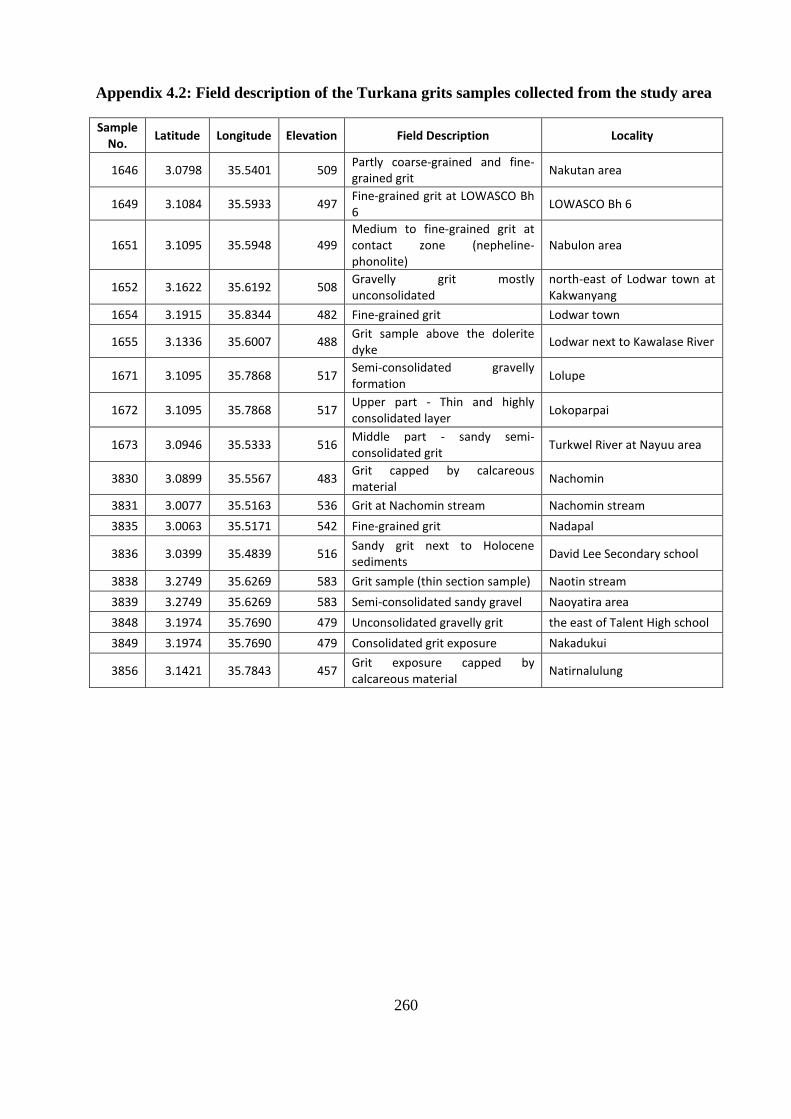
260

Appendix 4.2: Field description of the Turkana grits samples collected from the study area

Sample No.

Latitude Longitude Elevation Field Description Locality

1646 3.0798 35.5401 509 Partly coarse-grained and fine-grained grit

Nakutan area

1649 3.1084 35.5933 497 Fine-grained grit at LOWASCO Bh 6

LOWASCO Bh 6

1651 3.1095 35.5948 499 Medium to fine-grained grit at contact zone (nepheline-phonolite)

Nabulon area

1652 3.1622 35.6192 508 Gravelly grit mostly unconsolidated

north-east of Lodwar town at Kakwanyang

1654 3.1915 35.8344 482 Fine-grained grit Lodwar town

1655 3.1336 35.6007 488 Grit sample above the dolerite dyke

Lodwar next to Kawalase River

1671 3.1095 35.7868 517 Semi-consolidated gravelly formation

Lolupe

1672 3.1095 35.7868 517 Upper part - Thin and highly consolidated layer

Lokoparpai

1673 3.0946 35.5333 516 Middle part - sandy semi-consolidated grit

Turkwel River at Nayuu area

3830 3.0899 35.5567 483 Grit capped by calcareous material

Nachomin

3831 3.0077 35.5163 536 Grit at Nachomin stream Nachomin stream

3835 3.0063 35.5171 542 Fine-grained grit Nadapal

3836 3.0399 35.4839 516 Sandy grit next to Holocene sediments

David Lee Secondary school

3838 3.2749 35.6269 583 Grit sample (thin section sample) Naotin stream

3839 3.2749 35.6269 583 Semi-consolidated sandy gravel Naoyatira area

3848 3.1974 35.7690 479 Unconsolidated gravelly grit the east of Talent High school

3849 3.1974 35.7690 479 Consolidated grit exposure Nakadukui

3856 3.1421 35.7843 457 Grit exposure capped by calcareous material

Natirnalulung

261

Appendix 4.3: Field description of the Holocene sediments between Napuu and Lolupe, east

of Lodwar, Natir and at Turkwel Riverbank at Kakwanyang area

Lab No.

Latitude Longitude Elev

. Locality Field Description

Thickness (m)

Grain size

3820 3.1502 35.4910 509 Napuu/Lolupe (4, 000 YR BP)

Compacted light coloured sediment (A); No reaction with acid (10% HCl)

0.5 fine-

grained

3821 3.1502 35.4910 509 Dark coloured sediment (B); No reaction with acid (10% HCl)

1.5 fine-

grained

3822 3.1502 35.4910 509 Slightly light-coloured sediment (C); Fizzles with acid (10% HCl)

0.5 medium-grained

3823 3.1502 35.4910 509 Very fine-grained sandy layer (D); Fizzles with acid (10% HCl)

0.5 fine-

grained

3824 3.1229 35.5394 503 Lodwar East (4,

000 YR BP)

Dark coloured calcite layer (A); Fizzles with acid (10% HCl)

0.5 medium-grained

3825 3.1229 35.5394 503 Light-coloured sediment with calcite grains (B); Fizzles with acid (10% HCl)

1.5 fine-

grained

3826 3.0857 35.5573 510 Natir (4, 000 YR

BP)

Bottom layer (C) silty gravel; Fizzles with acid (10% HCl)

1 coarse- grained

3827 3.0857 35.5573 510

Middle layer (B) light coloured bed - absent quartz grains; No reaction with acid (10% HCl)

0.5 medium-grained

3829 3.0857 35.5573 510 The top layer (A) red-brown sediment; Fizzles with acid (10% HCl)

0.5 fine-

grained

3852 3.1830 35.8036 451

Turkwel Riverbank at Kakwanyang

(10,000 YR BP)

Layer A Fe-dominant; No reaction with acid (10% HCl)

1.5 fine-

grained

3853 3.1830 35.8036 451 Layer B- light coloured silty gravel; Fizzles with acid (10% HCl)

1 medium to fine

3854 3.1417 35.7358 496 Layer C – Clays; Fizzles with acid (10% HCl)

0.5 fine-

grained

3855 3.1420 35.7838 461

Layer D -Very fine-grained light-coloured bed with calcite grains; Fizzles with acid (10% HCl)

1.5 fine-

grained

262

Appendix 4.4: Field description of the Sandstone outcrops in the study area

Sample No.

Latitude Longitude Elev. Lab No.

Field Description Thickness

1645 3.0946 35.5336 516 1645 Sandstone with shale at Nadapal 0.5

1658 3.1136 35.5810 497 1658 Gravelly calcite-cemented sandstone at Nakwamekwi

0.3

1659 3.1136 35.5810 497 1659 Fine-grained sandstone with laminations 0.4

1668 3.1304 35.8579 460 1668 Coarser sandstone and gravel at Turkwel River east of Natir

0.3

1669 3.1304 35.8579 460 1669 Pebbly sandstone 0.2

1670 3.1095 35.7868 517 1670 Greenish fine-grained sandstone 1.8

1675 3.1420 35.8630 429 1675 White moist sandstone with Fe stain 0.2

1676 3.1420 35.8630 429 1676 Weakly unconsolidated coarse sandstone with gravel-sized clasts

0.5

1678 3.1420 35.8630 429 1678 White sandstone mixed with thin clay layers 0.50-0.70

3832 3.0077 35.5163 536 3832 Conglomeratic sandstone at Nachomin 0.4

3833 3.0063 35.5171 542 3833 Grey gravelly sandstone 0.4

3842 3.2748 35.5944 582 3842 Altered sandstone near Nabuelpus 0.7

3847 3.1427 35.7389 441 3847 Micaceous sandstone with clays located at natir

0.5

3850 3.1830 35.8036 451 3850 Unconsolidated gravelly sandstone 0.3

3858 3.1263 35.6475 462 3858 Fine-grained laminated sandstone 0.5

Appendix 4.5: Field description of conglomerate and grainstone samples

Lab No. Field Description Latitude Longitude Elevation Occurrence

1657 Grainstone -medium-fine grained 3.13044 35.85792 460 Rock outcrop at Natir

1667 Pebbly grainstone 3.13044 35.85792 460 Rock outcrop at Natir

1677 Conglomerate grading to silty grains 3.14196 35.86303 429 Layer capped the Turkana Grit at contact zone with nepheline phonolite

3857

Conglomerate grading to fine-grained with coarsening-upward bedding structures. Sediment cemented by calcium carbonate

3.14179 35.78517 462 Layer occurring within the sandstone unit

263

Appendix 4.6: Field description of volcanic rocks (augite basalt, nepheline-phonolite, and

dolerite dyke found in Turkana grits and basement rocks

Field Description

Augite Basalt

Nepheline- Phonolite

Nepheline- Phonolite

Nepheline Phonolite

Dolerite (TG) Dolerite (MB)

Lab No. 1648 1650 1653 1674 1656 3845

Latitude 3.1878 3.1139 3.1093 3.1138 3.1336 3.2748

Longitude 35.8381 35.5858 35.5947 35.5856 35.6007 35.5944

Elevation 497 502 498 497 488 582

Colour White-grey Grey-black Light coloured Black Dark grey to black Black-coloured

Texture Well-polished fine-grained surface

Fine to medium and unweathered fine-grained

Medium to coarse-grained, highly brecciated phonolite

Fine-grained

Medium to coarse-grained with Ophitic texture

fine-grained

Mineralogy A mixture of lava and sand

Tiny quartz crystals, haematite,

Prism-shaped minerals, quartz grains and haematite

Visible haematite and quartz grains

Plagioclase and pyroxene minerals with inclusions of the grits indicating the Turkana Grit is older

Deformed minerals and not visible

Occurrence Occurred on a volcanic hill east of Talent High school

Occurred on the Ngapoi Hills and comprised the volcanic cones within Lodwar town.

Formed contact with Turkana grit at Nabulon and is highly weathered

Collected on one of the cone-shaped features in Lodwar

Dyke in the Turkana grits displaying contact metasomatism features

Dyke in the Basement system

264

Appendix 4.7: Results of the whole rock analysis for samples collected from the study area (1645 -3858)

Rock Type Lab No. Field Code

Latitude Longitude Elev. SIO2 Al2O3 CaO MgO Na2O K2O TiO2 MnO Fe2O3 LOI

Alluvial 3851 Stop 93B 3.1830 35.8036 451 74.64 10.39 3.15 3.97 0.91 1.81 0.19 0.07 2.51 1.14

Augite Basalt 1648 Lod_002 3.1878 35.8381 497 53.79 18.00 5.69 3.22 0.64 2.06 1.09 0.12 6.08 9.22

Conglomerate 1677 Lod_033 3.1420 35.8630 429 71.60 9.72 4.99 2.25 0.79 2.13 0.31 0.09 2.03 5.99

Conglomerate 3857 Stop 133 3.1418 35.7852 462 60.07 9.15 12.15 0.04 1.70 3.52 0.26 0.70 2.51 8.68

Dolerite (MB) 3845 Stop 71 3.2748 35.5944 582 74.09 4.98 4.99 7.31 0.15 0.94 0.35 0.16 5.01 1.46

Dolerite (TG) 1656 Lod/010 3.1336 35.6007 488 50.59 15.87 4.70 1.71 0.27 7.01 1.89 0.28 8.12 8.62

Grainstone 1657 Lod_011 3.1304 35.8579 460 58.07 5.80 23.00 0.02 0.20 1.06 0.18 0.32 1.50 9.83

Grainstone 1667 Lod/023 3.1304 35.8579 460 64.30 8.30 7.84 5.19 0.73 2.95 0.15 0.13 1.13 9.13

Holocene sediments 3820 Stop 5A 3.1502 35.4910 509 66.90 16.05 2.74 1.50 0.15 2.43 0.76 0.10 3.78 5.50

Holocene sediments 3821 Stop 5B 3.1502 35.4910 509 55.10 14.70 2.55 1.47 0.10 1.87 1.34 0.19 7.70 14.16

Holocene sediments 3822 Stop 5C 3.1502 35.4910 509 51.80 16.42 2.62 0.11 0.17 1.84 1.24 0.20 7.71 17.09

Holocene sediments 3823 Stop 5D 3.1502 35.4910 509 80.85 10.92 2.61 0.12 0.12 1.68 0.14 0.17 1.11 2.07

Holocene sediments 3824 Stop 8A 3.1229 35.5394 503 57.97 16.52 2.06 1.37 0.14 1.39 0.94 0.12 7.97 11.26

Holocene sediments 3825 Stop 8B 3.1229 35.5394 503 69.97 11.89 5.34 1.97 0.09 2.02 0.43 0.08 3.14 4.10

Holocene sediments 3826 Stop 14A 3.0857 35.5573 510 24.91 4.89 27.15 7.01 0.08 0.72 0.27 0.30 2.14 32.00

Holocene sediments 3827 Stop 14B 3.0857 35.5573 510 12.89 2.01 45.78 0.07 0.04 0.06 0.14 0.52 1.99 36.31

Holocene sediments 3829 Stop 14C 3.0857 35.5573 510 68.97 10.21 1.82 2.67 0.05 1.81 0.62 0.09 4.73 8.48

Holocene sediments 3852 Stop 93C 3.1830 35.8036 451 48.79 18.90 1.25 1.93 1.30 3.24 1.20 0.14 9.53 13.16

Holocene sediments 3853 Stop 93D 3.1830 35.8036 451 43.69 18.70 1.01 0.08 1.96 3.41 1.41 0.17 13.15 15.97

Holocene sediments 3854 Stop 126 3.1417 35.7358 496 46.51 13.95 8.15 3.05 0.99 2.41 0.14 0.15 6.51 16.72

Holocene sediments 3855 Stop 130 3.1420 35.7838 461 46.07 9.87 19.50 2.87 0.87 1.57 0.75 0.60 3.90 12.91

Basement 3841 Stop 50 3.2748 35.5944 582 53.71 18.20 1.52 1.07 4.03 6.52 0.19 0.27 3.92 9.63

Basement 3843 Stop 50 3.2748 35.5944 582 52.83 19.95 2.15 0.01 4.93 5.87 0.18 0.25 4.31 8.66

Basement 3846 Stop 71 2.8575 35.6146 616 53.21 19.89 2.49 0.09 5.01 5.50 0.23 0.24 4.49 8.84

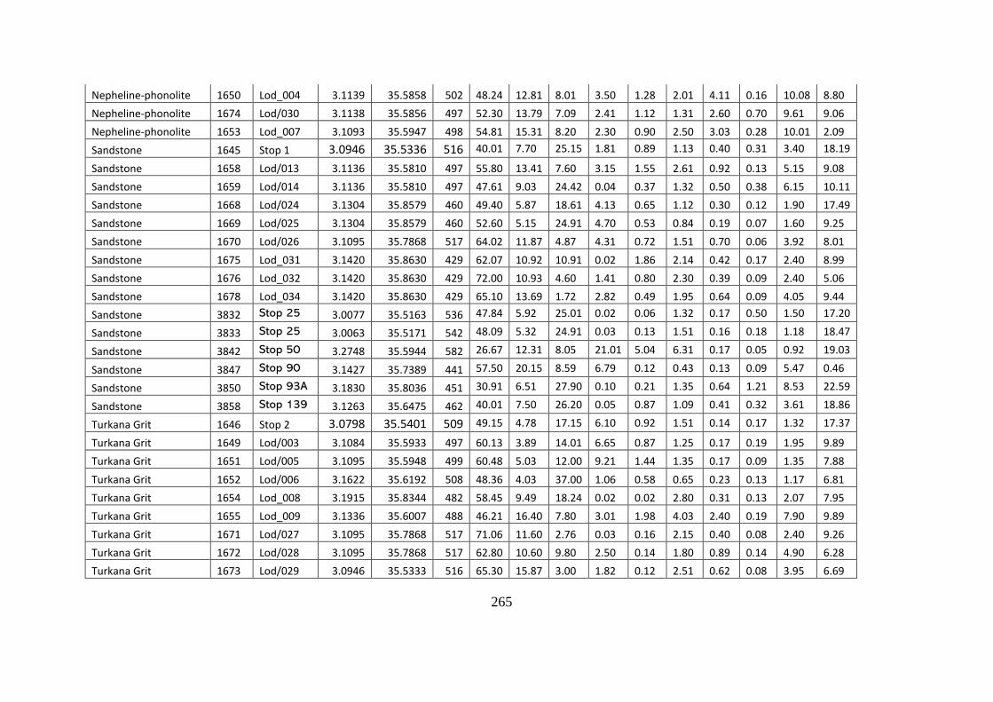
265

Nepheline-phonolite 1650 Lod_004 3.1139 35.5858 502 48.24 12.81 8.01 3.50 1.28 2.01 4.11 0.16 10.08 8.80

Nepheline-phonolite 1674 Lod/030 3.1138 35.5856 497 52.30 13.79 7.09 2.41 1.12 1.31 2.60 0.70 9.61 9.06

Nepheline-phonolite 1653 Lod_007 3.1093 35.5947 498 54.81 15.31 8.20 2.30 0.90 2.50 3.03 0.28 10.01 2.09

Sandstone 1645 Stop 1 3.0946 35.5336 516 40.01 7.70 25.15 1.81 0.89 1.13 0.40 0.31 3.40 18.19

Sandstone 1658 Lod/013 3.1136 35.5810 497 55.80 13.41 7.60 3.15 1.55 2.61 0.92 0.13 5.15 9.08

Sandstone 1659 Lod/014 3.1136 35.5810 497 47.61 9.03 24.42 0.04 0.37 1.32 0.50 0.38 6.15 10.11

Sandstone 1668 Lod/024 3.1304 35.8579 460 49.40 5.87 18.61 4.13 0.65 1.12 0.30 0.12 1.90 17.49

Sandstone 1669 Lod/025 3.1304 35.8579 460 52.60 5.15 24.91 4.70 0.53 0.84 0.19 0.07 1.60 9.25

Sandstone 1670 Lod/026 3.1095 35.7868 517 64.02 11.87 4.87 4.31 0.72 1.51 0.70 0.06 3.92 8.01

Sandstone 1675 Lod_031 3.1420 35.8630 429 62.07 10.92 10.91 0.02 1.86 2.14 0.42 0.17 2.40 8.99

Sandstone 1676 Lod_032 3.1420 35.8630 429 72.00 10.93 4.60 1.41 0.80 2.30 0.39 0.09 2.40 5.06

Sandstone 1678 Lod_034 3.1420 35.8630 429 65.10 13.69 1.72 2.82 0.49 1.95 0.64 0.09 4.05 9.44

Sandstone 3832 Stop 25 3.0077 35.5163 536 47.84 5.92 25.01 0.02 0.06 1.32 0.17 0.50 1.50 17.20

Sandstone 3833 Stop 25 3.0063 35.5171 542 48.09 5.32 24.91 0.03 0.13 1.51 0.16 0.18 1.18 18.47

Sandstone 3842 Stop 50 3.2748 35.5944 582 26.67 12.31 8.05 21.01 5.04 6.31 0.17 0.05 0.92 19.03

Sandstone 3847 Stop 90 3.1427 35.7389 441 57.50 20.15 8.59 6.79 0.12 0.43 0.13 0.09 5.47 0.46

Sandstone 3850 Stop 93A 3.1830 35.8036 451 30.91 6.51 27.90 0.10 0.21 1.35 0.64 1.21 8.53 22.59

Sandstone 3858 Stop 139 3.1263 35.6475 462 40.01 7.50 26.20 0.05 0.87 1.09 0.41 0.32 3.61 18.86

Turkana Grit 1646 Stop 2 3.0798 35.5401 509 49.15 4.78 17.15 6.10 0.92 1.51 0.14 0.17 1.32 17.37

Turkana Grit 1649 Lod/003 3.1084 35.5933 497 60.13 3.89 14.01 6.65 0.87 1.25 0.17 0.19 1.95 9.89

Turkana Grit 1651 Lod/005 3.1095 35.5948 499 60.48 5.03 12.00 9.21 1.44 1.35 0.17 0.09 1.35 7.88

Turkana Grit 1652 Lod/006 3.1622 35.6192 508 48.36 4.03 37.00 1.06 0.58 0.65 0.23 0.13 1.17 6.81

Turkana Grit 1654 Lod_008 3.1915 35.8344 482 58.45 9.49 18.24 0.02 0.02 2.80 0.31 0.13 2.07 7.95

Turkana Grit 1655 Lod_009 3.1336 35.6007 488 46.21 16.40 7.80 3.01 1.98 4.03 2.40 0.19 7.90 9.89

Turkana Grit 1671 Lod/027 3.1095 35.7868 517 71.06 11.60 2.76 0.03 0.16 2.15 0.40 0.08 2.40 9.26

Turkana Grit 1672 Lod/028 3.1095 35.7868 517 62.80 10.60 9.80 2.50 0.14 1.80 0.89 0.14 4.90 6.28

Turkana Grit 1673 Lod/029 3.0946 35.5333 516 65.30 15.87 3.00 1.82 0.12 2.51 0.62 0.08 3.95 6.69

266

Turkana Grit 3830 Stop 15 3.0899 35.5567 483 24.51 3.41 38.15 0.05 0.03 0.54 0.23 0.71 2.73 29.49

Turkana Grit 3831 Stop 24 3.0077 35.5163 536 60.80 4.81 4.31 0.04 0.09 0.94 0.32 0.31 2.71 24.91

Turkana Grit 3835 Stop 39 3.0063 35.5171 542 56.92 10.98 14.12 0.03 0.04 2.53 0.17 0.37 1.73 12.75

Turkana Grit 3836 Stop 39 3.0399 35.4839 516 70.86 12.15 3.15 2.01 0.11 2.09 0.51 0.08 3.41 5.47

Turkana Grit 3838 Stop 49 3.2749 35.6269 583 62.77 10.98 7.15 3.02 0.21 2.03 0.41 0.32 3.21 8.85

Turkana Grit 3839 Stop 50 3.2749 35.6269 583 45.70 9.12 11.72 8.71 0.09 0.98 0.77 2.01 3.51 16.62

Turkana Grit 3848 Stop 91 3.1974 35.7690 479 53.70 4.21 30.14 6.01 0.20 0.61 0.19 0.15 1.81 1.88

Turkana Grit 3849 Stop 91 3.1974 35.7690 479 21.83 4.21 30.14 6.01 0.20 0.61 0.19 0.15 1.81 34.27

Turkana Grit 3856 Stop 132 3.1421 35.7843 457 40.09 4.20 15.80 9.15 0.57 1.12 0.18 0.19 1.65 25.87

267

Appendix 4.8: Results of the major elements obtained from X-fluorescence spectrometry (XRF) at ICRAF lab (1648-3858); the results

have been arranged in order of rock samples where “nd” refers to not detected while “-“ were not measured

Rock Type Lab No.

Field Code

Lat Long Elev. Na Mg Al P S K Ca Mn Fe

Alluvial 3851 Stop 93B 3.1830 35.8036 451 nd 0.95 5.96 0.04 0.09 0.84 0.16 0.09 7.83

Augite Basalt 1648 Lod_002 3.1878 35.8381 497 nd 1.26 4.70 0.18 nd 0.48 4.99 0.17 5.09

Conglomerate 1677 Lod_033 3.1420 35.8630 429 nd 1.08 3.98 0.02 0.01 0.19 2.63 0.05 2.06

Conglomerate 3857 Stop 133 3.1418 35.7852 462 0.00 2.20 1.45 0.04 0.02 0.16 14.86 0.22 0.99

Dolerite (MB) 3845 Stop 71 3.2748 35.5944 582 0.00 2.32 3.71 0.02 0.01 0.02 8.56 0.14 4.12

Dolerite (TG) 1656 Lod/010 3.1336 35.6007 488 - - - - - - - - -

Grainstone 1657 Lod_011 3.1304 35.8579 460 0.05 0.43 1.37 0.03 0.02 0.14 17.18 0.41 1.22

Grainstone 1667 Lod/023 3.1304 35.8579 460 - - - - - - - - -

Holocene sediments 3820 Stop 5A 3.1502 35.4910 509 nd 0.64 3.76 0.07 0.01 0.39 2.51 0.09 3.03

Holocene sediments 3821 Stop 5B 3.1502 35.4910 509 nd 0.73 4.87 0.07 0.00 0.64 1.88 0.14 5.16

Holocene sediments 3822 Stop 5C 3.1502 35.4910 509 nd 0.69 4.69 0.06 nd 0.62 1.88 0.14 4.80

Holocene sediments 3823 Stop 5D 3.1502 35.4910 509 0.11 0.09 1.72 0.03 0.01 0.11 2.50 0.03 1.23

Holocene sediments 3824 Stop 8A 3.1229 35.5394 503 nd 1.18 5.32 0.04 0.18 0.69 1.49 0.09 5.67

Holocene sediments 3825 Stop 8B 3.1229 35.5394 503 nd 0.84 3.01 0.05 0.00 0.26 4.93 0.07 2.40

Holocene sediments 3826 Stop 14A 3.0857 35.5573 510 0.00 2.83 1.62 0.03 0.02 0.09 18.98 0.23 1.18

Holocene sediments 3827 Stop 14B 3.0857 35.5573 510 nd 0.34 1.13 nd 0.02 0.07 25.23 0.87 0.88

Holocene sediments 3829 Stop 14C 3.0857 35.5573 510 nd 1.36 4.04 0.02 nd 0.27 1.25 0.05 3.32

Holocene sediments 3852 Stop 93C 3.1830 35.8036 451 0.00 1.80 4.23 0.06 0.06 0.36 5.22 0.12 3.96

Holocene sediments 3853 Stop 93D 3.1830 35.8036 451 nd 0.75 1.79 0.09 0.07 0.26 14.79 0.71 2.29

Holocene sediments 3854 Stop 126 3.1417 35.7358 496 0.00 4.53 2.06 0.03 0.08 0.12 13.32 0.13 1.17

Holocene sediments 3855 Stop 130 3.1420 35.7838 461 0.19 0.37 1.31 0.08 0.02 0.40 9.36 0.26 1.84

Basement 3841 Stop 50 3.2748 35.5944 582 0.00 1.96 1.71 0.03 0.07 0.37 12.63 0.07 1.12

Basement 3843 Stop 50 3.2748 35.5944 582 0.00 2.89 1.82 0.05 nd 0.17 5.34 0.18 4.26

Basement 3846 Stop 71 2.8575 35.6146 616 0.00 2.42 3.38 0.03 0.01 0.14 7.82 0.20 6.32

268

Nepheline-phonolite 1650 Lod/004 3.1139 35.5858 502 0.22 nd 5.46 0.08 nd 0.52 1.69 0.13 3.62

Nepheline-phonolite 1674 Lod/030 3.1138 35.5856 497 - - - - - - - - -

Nepheline-phonolite 1653 Lod/007 3.1093 35.5947 498 0.00 1.37 3.87 0.33 nd 0.87 6.80 0.20 6.01

Sandstone 1645 Stop 1 3.0946 35.5336 516 - - - - - - - - -

Sandstone 1658 Lod/013 3.1136 35.5810 497 - - - - - - - - -

Sandstone 1659 Lod/014 3.1136 35.5810 497 - - - - - - - - -

Sandstone 1668 Lod/024 3.1304 35.8579 460 - - - - - - - - -

Sandstone 1669 Lod/025 3.1304 35.8579 460 - - - - - - - - -

Sandstone 1670 Lod/026 3.1095 35.7868 517 - - - - - - - - -

Sandstone 1675 Lod_031 3.1420 35.8630 429 nd 1.09 2.68 0.04 0.03 0.15 11.09 0.15 1.70

Sandstone 1676 Lod_032 3.1420 35.8630 429 nd 1.07 2.63 0.06 0.01 0.22 7.74 0.11 1.91

Sandstone 1678 Lod_034 3.1420 35.8630 429 nd 1.09 4.37 0.03 nd 0.30 1.18 0.05 3.68

Sandstone 3832 Stop 25 3.0077 35.5163 536 0.19 0.24 0.95 0.04 0.03 0.22 19.13 0.22 0.99

Sandstone 3833 Stop 25 3.0063 35.5171 542 0.22 0.24 0.94 0.03 0.04 0.21 18.21 0.22 0.97

Sandstone 3842 Stop 50 3.2748 35.5944 582 0.27 0.29 4.73 0.03 0.01 0.74 1.37 0.19 3.41

Sandstone 3847 Stop 90 3.1427 35.7389 441 0.00 2.67 1.49 0.01 0.08 0.07 19.70 0.15 0.97

Sandstone 3850 Stop 93A 3.1830 35.8036 451 nd 1.26 5.89 0.07 0.02 0.88 0.62 0.09 6.88

Sandstone 3858 Stop 139 3.1263 35.6475 462 0.00 3.91 2.04 0.05 0.02 0.12 12.65 0.11 0.97

Turkana Grit 1646 Stop 2 3.0798 35.5401 509 - - - - - - - - -

Turkana Grit 1649 Lod/003 3.1084 35.5933 497 - - - - - - - - -

Turkana Grit 1651 Lod/005 3.1095 35.5948 499 - - - - - - - - -

Turkana Grit 1652 Lod/006 3.1622 35.6192 508 - - - - - - - - -

Turkana Grit 1654 Lod_008 3.1915 35.8344 482 0.19 0.26 1.24 0.05 0.02 0.39 19.53 0.15 1.29

Turkana Grit 1655 Lod_009 3.1336 35.6007 488 nd 1.04 4.10 0.26 nd 0.84 6.25 0.27 6.32

Turkana Grit 1671 Lod/027 3.1095 35.7868 517 - - - - - - - - -

Turkana Grit 1672 Lod/028 3.1095 35.7868 517 - - - - - - - - -

Turkana Grit 1673 Lod/029 3.0946 35.5333 516 - - - - - - - - -

269

Turkana Grit 3830 Stop 15 3.0899 35.5567 483 nd 0.48 1.14 0.02 0.02 0.16 22.67 1.19 1.35

Turkana Grit 3831 Stop 24 3.0077 35.5163 536 nd 0.41 0.89 0.03 0.04 0.20 22.12 0.32 1.06

Turkana Grit 3835 Stop 39 3.0063 35.5171 542 0.19 0.35 1.49 0.03 0.02 0.39 11.41 0.36 1.50

Turkana Grit 3836 Stop 39 3.0399 35.4839 516 nd 0.74 3.39 0.04 nd 0.23 1.91 0.05 2.77

Turkana Grit 3838 Stop 49 3.2749 35.6269 583 0.00 3.38 2.62 0.05 0.01 0.10 9.08 0.18 2.22

Turkana Grit 3839 Stop 50 3.2749 35.6269 583 0.21 0.49 4.62 0.03 0.01 0.75 0.92 0.21 3.34

Turkana Grit 3848 Stop 91 3.1974 35.7690 479 nd 0.60 1.96 0.08 0.04 0.23 17.31 1.62 2.90

Turkana Grit 3849 Stop 91 3.1974 35.7690 479 nd 0.78 2.10 0.04 0.00 0.18 2.75 0.06 2.25

Turkana Grit 3856 Stop 132 3.1421 35.7843 457 nd 0.70 1.78 0.06 0.03 0.15 17.08 0.33 1.53

Appendix 4.9: Results of the trace elements obtained from X-fluorescence spectrometry (XRF) at ICRAF lab (1648-3858); the results have

been arranged in order of rock samples where “nd” refers to not detected while “-“were not measured

Rock Type Lab No.

Field Code

Lat Long Elev. Ti Cr Co Ni Cu Zn As Se Mo Pb

Alluvial 3851 Stop 93B 3.1830 35.8036 451 0.17 0.01 0.00 0.01 0.00 0.02 nd nd 0.00 nd

Augite Basalt 1648 Lod_002 3.1878 35.8381 497 0.26 0.01 0.00 0.00 0.00 0.01 nd 0.00 nd nd

Conglomerate 1677 Lod_033 3.1420 35.8630 429 0.04 0.00 nd 0.00 0.00 0.01 nd nd 0.00 nd

Conglomerate 3857 Stop 133 3.1418 35.7852 462 nd 0.01 nd 0.00 nd 0.01 nd nd 0.00 nd

Dolerite (MB) 3845 Stop 71 3.2748 35.5944 582 nd 0.03 0.00 0.00 nd 0.01 nd nd 0.00 nd

Dolerite (TG) 1656 Lod/010 3.1336 35.6007 488 - - - - - - - - - -

Grainstone 1657 Lod_011 3.1304 35.8579 460 nd 0.01 nd 0.00 nd 0.01 nd 0.00 0.00 nd

Grainstone 1667 Lod/023 3.1304 35.8579 460 - - - - - - - - - -

Holocene sediments 3820 Stop 5A 3.1502 35.4910 509 0.14 0.01 0.00 0.00 0.00 0.01 nd nd 0.00 nd

Holocene sediments 3821 Stop 5B 3.1502 35.4910 509 0.19 0.01 0.00 0.00 0.00 0.02 nd nd 0.00 nd

Holocene sediments 3822 Stop 5C 3.1502 35.4910 509 0.19 0.01 0.00 0.00 0.00 0.02 nd nd 0.00 nd

270

Holocene sediments 3823 Stop 5D 3.1502 35.4910 509 0.02 0.01 nd 0.00 0.00 0.01 nd nd 0.00 nd

Holocene sediments 3824 Stop 8A 3.1229 35.5394 503 0.13 0.01 0.00 0.00 0.01 0.02 nd nd 0.00 nd

Holocene sediments 3825 Stop 8B 3.1229 35.5394 503 0.05 0.01 0.00 0.00 nd 0.01 nd nd 0.00 nd

Holocene sediments 3826 Stop 14A 3.0857 35.5573 510 0.02 0.00 nd 0.00 nd 0.01 nd nd 0.00 nd

Holocene sediments 3827 Stop 14B 3.0857 35.5573 510 nd 0.01 nd 0.02 nd 0.01 nd 0.00 0.00 nd

Holocene sediments 3829 Stop 14C 3.0857 35.5573 510 0.06 0.01 0.00 0.00 0.00 0.01 nd nd 0.00 nd

Holocene sediments 3852 Stop 93C 3.1830 35.8036 451 0.10 0.01 0.00 0.00 0.02 0.02 nd nd 0.00 nd

Holocene sediments 3853 Stop 93D 3.1830 35.8036 451 0.10 0.01 0.00 0.00 0.00 0.01 nd nd 0.00 nd

Holocene sediments 3854 Stop 126 3.1417 35.7358 496 0.01 0.01 nd 0.00 nd 0.01 nd nd 0.00 nd

Holocene sediments 3855 Stop 130 3.1420 35.7838 461 0.01 0.01 0.00 0.00 0.00 0.01 nd nd 0.00 nd

Basement 3841 Stop 50 3.2748 35.5944 582 0.01 0.01 nd 0.00 0.03 0.01 nd nd 0.00 nd

Basement 3843 Stop 50 3.2748 35.5944 582 0.01 0.08 0.00 0.02 nd 0.01 nd nd 0.00 nd

Basement 3846 Stop 71 2.8575 35.6146 616 nd 0.08 0.00 0.01 nd 0.01 nd 0.00 0.00 nd

Nepheline-phonolite 1650 Lod_004 3.1139 35.5858 502 0.10 0.00 0.00 0.00 nd 0.02 nd 0.00 0.00 nd

Nepheline-phonolite 1674 Lod/030 3.1138 35.5856 497 - - - - - - - - - -

Nepheline-phonolite 1653 Lod_007 3.1093 35.5947 498 0.71 0.01 0.00 0.00 0.02 0.02 nd 0.00 nd nd

Sandstone 1645 Stop 1 3.0946 35.5336 516 - - - - - - - - - -

Sandstone 1658 Lod/013 3.1136 35.5810 497 - - - - - - - - - -

Sandstone 1659 Lod/014 3.1136 35.5810 497 - - - - - - - - - -

Sandstone 1668 Lod/024 3.1304 35.8579 460 - - - - - - - - - -

Sandstone 1669 Lod/025 3.1304 35.8579 460 - - - - - - - - - -

Sandstone 1670 Lod/026 3.1095 35.7868 517 - - - - - - - - - -

Sandstone 1675 Lod_031 3.1420 35.8630 429 0.01 0.00 nd 0.00 nd 0.01 nd nd 0.00 nd

Sandstone 1676 Lod_032 3.1420 35.8630 429 0.01 0.01 0.00 0.00 0.00 0.01 nd nd 0.00 nd

Sandstone 1678 Lod_034 3.1420 35.8630 429 0.07 0.01 0.00 0.00 0.00 0.01 nd nd 0.00 nd

Sandstone 3832 Stop 25 3.0077 35.5163 536 0.00 0.01 nd 0.00 nd 0.01 nd nd 0.00 nd

Sandstone 3833 Stop 25 3.0063 35.5171 542 0.01 0.01 nd 0.00 nd 0.01 nd nd 0.00 nd

271

Sandstone 3842 Stop 50 3.2748 35.5944 582 nd 0.00 0.00 0.00 nd 0.03 nd nd 0.00 nd

Sandstone 3847 Stop 90 3.1427 35.7389 441 0.01 0.00 nd 0.00 0.00 0.01 nd nd 0.00 nd

Sandstone 3850 Stop 93A 3.1830 35.8036 451 0.18 0.01 0.00 0.01 0.00 0.02 nd nd 0.00 nd

Sandstone 3858 Stop 139 3.1263 35.6475 462 nd 0.00 nd 0.00 0.00 0.01 nd nd 0.00 nd

Turkana Grit 1646 Stop 2 3.0798 35.5401 509 - - - - - - - - - -

Turkana Grit 1649 Lod/003 3.1084 35.5933 497 - - - - - - - - - -

Turkana Grit 1651 Lod/005 3.1095 35.5948 499 - - - - - - - - - -

Turkana Grit 1652 Lod/006 3.1622 35.6192 508 - - - - - - - - - -

Turkana Grit 1654 Lod_008 3.1915 35.8344 482 0.01 0.00 nd 0.00 nd 0.01 nd nd 0.00 nd

Turkana Grit 1655 Lod_009 3.1336 35.6007 488 0.74 0.01 0.00 0.00 0.01 0.02 nd 0.00 nd nd

Turkana Grit 1671 Lod/027 3.1095 35.7868 517 - - - - - - - - - -

Turkana Grit 1672 Lod/028 3.1095 35.7868 517 - - - - - - - - - -

Turkana Grit 1673 Lod/029 3.0946 35.5333 516 - - - - - - - - - -

Turkana Grit 3830 Stop 15 3.0899 35.5567 483 0.01 0.01 nd 0.00 nd 0.01 nd nd 0.00 nd

Turkana Grit 3831 Stop 24 3.0077 35.5163 536 0.02 0.01 0.00 0.00 nd 0.01 nd nd 0.00 nd

Turkana Grit 3835 Stop 39 3.0063 35.5171 542 0.01 0.01 0.00 0.00 0.00 0.01 nd nd 0.00 nd

Turkana Grit 3836 Stop 39 3.0399 35.4839 516 0.05 0.01 0.00 0.00 0.00 0.01 nd nd 0.00 nd

Turkana Grit 3838 Stop 49 3.2749 35.6269 583 0.08 0.01 0.00 0.00 0.01 0.01 nd nd 0.00 nd

Turkana Grit 3839 Stop 50 3.2749 35.6269 583 nd 0.00 0.00 0.00 nd 0.02 nd nd 0.00 nd

Turkana Grit 3848 Stop 91 3.1974 35.7690 479 0.07 0.01 0.00 0.01 nd 0.01 nd 0.00 0.00 nd

Turkana Grit 3849 Stop 91 3.1974 35.7690 479 0.00 0.01 0.00 0.00 nd 0.01 nd nd 0.00 nd

Turkana Grit 3856 Stop 132 3.1421 35.7843 457 0.04 0.01 nd 0.00 nd 0.01 nd nd 0.00 nd

272

Appendix 4.10: Results of the vertical electrical soundings for VES 1 to VES 15

AB/2 MN/2 VES 1 VES 3 VES 4 VES 5 VES 6 VES 7 VES 8 VES 9 VES 10 VES 11 VES 12 VES 13 VES 14 VES 15

Latitude 3.11233 3.10599 3.10567 3.10711 3.11173 3.11299 3.10144 3.09746 3.10813 3.11773 3.12451 3.08444 3.0767 3.07674

Longitude 35.5964 35.6418 35.6432 35.6613 35.6528 35.6535 35.6673 35.7147 35.7192 35.7104 35.7244 35.5717 35.5663 35.5708

Elevation 474 479 472 467 476 474 470 485 482 466 457 492 494 501

1.6 0.5 1054 1065 1550 3822 265.1 134.7 2619 55.2 101.8 15.73 69.18 84.2 275.2 86.4

2 0.5 638.1 1039 1499 3401 169.4 103.4 2597 50.7 100.5 17.86 80.42 95.6 253.9 72

2.5 0.5 342.8 1001 1426 3209 135.5 80.89 2560 47 98.58 20.95 92.62 105 232.3 58.3

3.2 0.5 161.7 938.5 1307 2883 140.6 66.5 2480 44 95.38 26.04 106.6 107 209.1 44

4 0.5 96.01 866.5 1173 2317 161.4 62.5 2356 40.8 91.99 32.24 119.6 104 190.3 39.7

5 0.5 74.72 785 1029 1690 187.7 64.51 2158 35.7 89.29 40.2 132.5 100 172.4 36.2

6.3 0.5 69.95 697.3 885 1263 215.9 71.48 1857 31.7 89.34 50.64 145.4 88.3 151.9 36.7

8 0.5 68.17 606.9 754.6 943 244.8 83.11 1451 29.2 94.87 64.29 158.3 75 126.5 37

10 0.5 67.12 520.5 647 758 269.2 97.62 1032 26.3 106.6 80.35 170.2 64.8 98.42 39.5

13 0.5 65.92 411.7 522.3 583 292.5 118.6 584.5 23.3 128.4 104.4 185.2 62.3 64.22 42

16 0.5 64.64 322.2 417.8 423 305.6 137.7 325.5 19.6 151 128.5 199.7 64 40.86 43.1

20 0.5 62.59 231.8 303.8 238 314.5 160.3 155.3 16.5 179.4 160.6 220.5 68.3 23.01 40.7

25 0.5 59.42 159.9 201.9 108 319.7 185 70.95 13.5 211.5 200.7 250.6 83.1 13.44 36.5

32 10 54.28 109.1 125.5 48.3 324.7 214.1 31.05 10.7 250.6 256.8 299.8 106 8.976 30.4

40 10 48.2 85.32 91.96 28.6 333.1 241.7 16.54 8.02 287.9 320.9 363.4 127 7.733 19.3

50 10 41.32 73.68 83.52 23.4 350.4 270.3 10.85 7.71 324.9 400.8 448.3 147 7.274 16.7

63 10 67.23 89.03 21 382.3 301.5 8.855 8.12 360.1 504.7 562.2 177 6.965 12.6

80 10 61.9 99.19 19.3 434.6 336.9 8.616 8.12 386.9 640.3 712 215 6.68 11.2

100 10 57.24 109.4 18.9 502.4 376.1 9.054 8.74 394.1 799.4 887.9 6.443 12.3

130 10 52.32 120.5 19.3 604.4 436.4 10.18 9.5 391.4 1038 1150 6.213 13.5

160 10 49.21 128.8 19.5 698.8 502.6 11.67 10 1275 1411 6.078 17.6

200 10 46.82 20.7 810.5 600.8 13.98 11.3 1590 1756 5.975 21.3

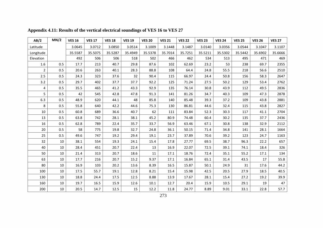
273

Appendix 4.11: Results of the vertical electrical soundings of VES 16 to VES 27

AB/2 MN/2 VES 16 VES 17 VES 18 VES 19 VES 20 VES 21 VES 22 VES 23 VES 24 VES 25 VES 26 VES 27

Latitude 3.0645 3.0712 3.0850 3.0514 3.1009 3.1448 3.1487 3.0140 3.0356 3.0544 3.1047 3.1107

Longitude 35.5587 35.5075 35.5287 35.4949 35.5378 35.7014 35.7251 35.5211 35.5302 35.5442 35.6902 35.6666

Elevation 492 506 506 518 502 466 462 534 513 495 471 469

1.6 0.5 17.7 213 40.7 29.8 87.6 102 62.69 23.2 53 238 69.7 2355

2 0.5 20.6 263 40.1 28.3 88.8 108 64.4 24.8 55.5 218 56.6 2510

2.5 0.5 24.3 323 37.6 32 90.4 115 66.97 24.4 50.8 156 58.3 2647

3.2 0.5 29.7 402 37.7 37.7 92.2 125 71.24 27.5 50.2 129 53.4 2762

4 0.5 35.5 465 41.2 43.3 92.9 135 76.14 30.8 43.9 112 49.5 2836

5 0.5 42 545 42.8 47.8 91.3 141 81.26 34.7 40.3 109 47.3 2878

6.3 0.5 48.9 620 44.1 48 85.8 140 85.48 39.3 37.2 109 43.8 2881

8 0.5 55.8 640 42.2 44.6 75.3 130 86.81 44.6 32.4 115 43.8 2827

10 0.5 60.8 689 36.6 40.7 62 111 83.84 52.3 30.3 117 41.1 2704

13 0.5 63.8 742 28.1 38.1 45.2 80.9 74.48 60.4 30.2 135 37.7 2436

16 0.5 62.8 789 22.4 35.7 33.7 56.9 63.46 67.1 30.8 138 32.9 2112

20 0.5 58 775 19.8 32.7 24.8 36.1 50.15 71.4 34.8 141 28.1 1664

25 0.5 49.6 747 19.2 29.4 19.1 23.7 37.89 70.6 39.2 123 24.7 1163

32 10 38.1 554 19.3 24.1 15.4 17.8 27.77 69.5 38.7 96.3 22.2 657

40 10 28.4 451 20.7 22.4 13 16.9 22.07 72.5 39.1 74.1 18.4 326

50 10 21.4 313 20.7 18.6 11 17.1 18.76 72.4 35.1 55.2 17.1 134

63 10 17.7 216 20.7 15.2 9.37 17.1 16.84 65.1 31.4 43.5 17 55.8

80 10 16.9 103 20.2 13.6 8.39 16.5 15.87 50.1 24.9 31 17.6 44.2

100 10 17.5 55.7 19.1 12.8 8.21 15.4 15.98 42.5 20.5 27.9 18.5 40.5

130 10 18.8 24.4 17.5 12.5 8.88 13.9 17.67 28.1 15.4 27.2 19.2 39.9

160 10 19.7 16.5 15.9 12.6 10.1 12.7 20.4 15.9 10.5 29.1 19 47

200 10 20.5 14.7 12.5 15 12.2 11.8 24.77 8.89 9.01 33.1 22.8 57.7

274

Appendix 4.12: VES graphs for VES 17 to 20 carried out on section A of the LAAS around Nadapal and Naoyatira areas

275

Appendix 4.13: VES graphs carried out in section B of the LAAS between Kakemera and

Nachomin areas

Appendix 4.14: VES graphs for section C of the LAAS around Kakwanyang and Nang'omo

areas

277

Appendix 4.15: VES graphs of section d of the LAAS covering Napuu, Lolupe and Nayuu

areas

VES 9

Appendix 4.16: Results for oxygen-18, deuterium and tritium for rainfall and surface water (Turkwel River = TR, Kawalase River = KR,

water pans = pan, scoop holes = SH, Eliye sprong and Lake Turkana = LT) samples in Lodwar and its environs

No Sample_Date Sample ID Lat Long Elevation

(m) Sample Code

Type 18O 2H TU

1 18/02/2018

Rain Sample (REACH Office)

3.101107°

35.602050°

517 2442 Rain -1.33 7.4 1.7

2 18/02/2018

Turkwel at KEFRI near Bh 1

3.1124 35.5990 485 2440 TR 0.37 6.6 2.1

3 18/02/2018 Turkwel at Kangangetei 3.1440 35.8593 410 2437 TR 0.89 9.8 nm

4 18/02/2018 Turkwel at Nangolekuruk 3.1096 36.0502 387 2441 TR 0.90 7.6 nm

5 18/02/2018 Turkwel_Namupoth 3.1590 35.8243 430 2438 TR 0.06 6.5 nm

6 21/05/2018 Kalawase Tri 3.1302 35.5219 510 3293 KR 0.25 2.6 nm

7 21/05/2018 Nakutan Pan 3.1249 35.4871 511 3296 Pan -3.01 -22.5 nm

8 27/05/2018 Monti Water pan 3.1924 35.6387 512 3320 Pan -4.40 -33.9 nm

9 29/05/2018 Namuthia Water Pan 3.1954 35.6732 489 3332 Pan -2.67 -15.9 nm

10 30/05/2018 Nakariong'ora Water Pan 3.2217 35.7798 482 3342 Pan -2.52 -10.7 nm

11 03/06/2018 Kerio water Pan 3.0909 35.6851 482 3375 Pan 0.19 0.9 nm

12 21/05/2018 Nakutan Lagga 1 3.1338 35.4834 505 3294 SH -1.57 -14.0 nm

13 21/05/2018 Kalawase Lagga 3.1502 35.4910 510 3295 SH -1.43 -5.2 nm

14 01/06/2018 Monti Lagga 3.2383 35.6293 516 3324 SH -3.27 -11.4 nm

15 28/05/2018 Kawalase Bridge 3.1329 35.6011 462 3326 SH -3.65 -23.7 nm

16 28/05/2018 Nakutan Lagga 2 3.1331 35.4997 497 3327 SH -3.95 -21.6 nm

17 02/06/2018 Monti Lagga 3.1672 35.6496 492 3330 SH -2.63 -6.9 nm

18 31/05/2018 Nakadukui Lagga 3.1824 35.7582 419 3347 SH -2.21 -8.0 nm

19 31/05/2018 Chokochok lagga 3.1580 35.7458 459 3348 SH -1.96 -2.4 nm

20 18/02/2018 Eliye Springs 3.2525 36.0207 382 2436 Spring -2.51 -7.4 nm

21 18/02/2018 Lake Turkana_Eliye 3.2536 36.0217 363 2461 LT 5.41 41.3 1.7

22 18/02/2018 Lake_Turkwel_Delta 3.0584 36.1433 373 2462 LT 6.60 42.4 1.8

279

Appendix 4.17: Results for oxygen-18, deuterium and tritium for groundwater samples in shallow alluvial aquifer (SAA), Turkana grit

shallow aquifer (TGSA), intermediate aquifer (IA), deep aquifer (DA), and for wells with unknown depth (DU); (nm = not measured)

No. Sample_Date SampleID Aquifer Lat Long Elevation

(m) Sample Code

Type 18O 2H TU

1 31/05/2018 Akibululu Hp SAA 3.1527 35.7678 456 3344 Hp -0.50 2.7 1.8

2 03/06/2018 Bh 1A SAA 3.1131 35.5980 497 3381 Bh -2.89 -9.5 nm

3 03/06/2018 Bh 1B SAA 3.1127 35.5984 501 3380 Bh -2.92 -13.1 nm

4 03/06/2018 Bh 2C SAA 3.1108 35.5928 493 3382 Bh 0.25 3.5 nm

5 03/06/2018 Bh 3 SAA 3.1133 35.6005 489 3383 Bh -1.33 -0.1 1.8

6 03/06/2018 Bh 5 SAA 3.1117 35.5972 486 3387 Bh -0.41 4.2 nm

7 03/06/2018 Bh 7 SAA 3.1077 35.5824 482 3384 Bh -0.51 3.6 1.8

8 03/06/2018 Bh 9 SAA 3.1122 35.5963 489 3388 Bh -0.63 2.2 1.6

9 24/05/2018 Kakemera Pri Hp SAA 3.0860 35.5621 524 3300 Hp -1.28 1.4 nm

10 03/06/2018 KFS Hp SAA 3.1128 35.6002 500 3390 Hp -2.24 -10.5 1.1

11 31/05/2018 Locher A Akalale Hp SAA 3.1525 35.7583 415 3298 Hp -0.85 4.5 nm

12 31/05/2018 Lodwar Mixed Pri 1 SAA 3.1186 35.6104 500 3349 Hp -0.24 3.9 1.4

13 31/05/2018 Lodwar Mixed Pri 2 SAA 3.1186 35.6116 496 3355 Hp -0.51 4.7 nm

14 28/05/2018 Lokipetot Bh SAA 3.0892 35.5488 500 3329 Bh -1.02 0.0 nm

15 01/06/2018 Lolupe 3 Hp SAA 3.1063 35.6809 434 3360 Hp -1.68 -5.2 1.3

16 01/06/2018 Nabulon Drinking water well SAA 3.1363 35.7325 486 3365 Hp -0.60 4.1 nm

17 26/05/2018 Nadapal Hp SAA 3.0684 35.5092 508 3313 Hp -0.28 2.5 1.5

18 30/05/2018 Nakwalele Hp 2 SAA 3.1322 35.6312 460 3338 Hp -0.74 0.8 1.3

19 26/05/2018 Nakwamekwi Pri Bh SAA 3.1115 35.5790 509 3307 Bh -1.29 -1.4 nm

20 26/05/2018 Naregai Bh SAA 3.0992 35.5584 477 3312 Bh -1.92 -3.4 nm

21 31/05/2018 Nasenyanait Hp 2 SAA 3.1224 35.6230 480 3351 Hp 0.25 5.8 2.2

22 31/05/2018 Natotol SAA 3.1178 35.6176 482 3354 Hp -0.53 4.7 nm

23 05/06/2018 Al Noor Community Hp TGSA 3.1218 35.5912 528 3396 Hp -2.35 -9.9 <0.8

24 29/05/2018 Bokotom Hp TGSA 3.1689 35.6934 481 3334 Hp -2.53 -10.4 <0.8

25 05/06/2018 Loyo Pri Hp TGSA 3.1219 35.5811 514 3399 Hp -2.53 -10.7 nm

280

26 29/05/2018 Namuthia Hp TGSA 3.1792 35.7004 493 3345 Hp -3.05 -13.1 <0.8

27 29/05/2018 Talent High Sch Hp TGSA 3.1918 35.6755 502 3331 Hp -3.33 -14.8 nm

28 04/06/2018 Trumpet of Hope Ministries TGSA 3.1206 35.5829 491 3394 Hp -1.93 -8.8 <0.8

29 03/06/2018 Bh 6 IA 3.1080 35.5935 499 3389 Bh -1.44 -3.7 nm

30 30/05/2018 Chokochok Pry IA 3.1423 35.7394 453 3341 Hp 0.07 4.5 1.9

31 03/06/2018 Chukultom Hp IA 3.1183 35.5802 497 3386 Hp -2.82 -8.7 nm

32 05/06/2018 Comboni Girls IA 3.1146 35.5643 532 3398 Bh -2.54 -9.9 nm

33 01/06/2018 Eleleia Pri Hp IA 3.1247 35.7357 465 3364 Hp -2.77 -9.4 <0.8

34 24/05/2018 Kakemera Church IA 3.0654 35.5616 513 3302 Hp -2.61 -7.9 1.0

35 26/05/2018 Kochoda Hp IA 3.1040 35.5631 482 3391 Hp -2.24 -5.7 nm

36 25/05/2018 Limyounsim Bh IA 2.9994 35.5137 549 3309 Bh -2.89 -10.7 <0.8

37 01/06/2018 Loporkou-Eleleai Hp IA 3.1231 35.7491 486 3366 Hp -3.92 -9.7 nm

38 25/05/2018 Nachomin Bh IA 3.0131 35.5195 547 3306 Bh -2.74 -10.6 <0.8

39 26/05/2018 Nadapal Supply bh IA 3.0734 35.5095 498 3314 Bh -1.91 -5.8 nm

40 26/05/2018 Nagis Bakhita Bh IA 3.0440 35.4902 527 3317 Bh -2.67 -8.6 <0.8

41 26/05/2018 Nakwamekwi Hp IA 3.1101 35.5759 509 3310 Hp -2.40 -7.6 nm

42 02/06/2018 Napuu 2 IA 3.1061 35.6409 490 3373 Bh -1.79 -4.1 nm

43 02/06/2018 Napuu 4 Resample IA 3.1053 35.6417 480 3374 Bh -0.63 0.3 1.5

44 27/05/2018 Nareng'elup 2 IA 3.2379 35.6301 535 3323 Hp -2.63 -10.8 nm

45 01/06/2018 Natot Pri Bh IA 3.1143 35.6452 508 3357 Bh -1.47 -0.4 nm

46 04/06/2018 Nauren Puu IA 3.0888 35.5359 516 3392 Bh -0.50 -0.9 nm

47 01/06/2018 Nayuu Hp 4 IA 3.1066 35.7111 491 3368 Hp -3.09 -7.0 nm

48 01/06/2018 Nayuu Hp Resample IA 3.1082 35.7214 475 3363 Hp -2.56 -11.3 nm

49 02/06/2018 Napuu 1 Resample DA 3.1061 35.6407 502 3372 Bh -1.17 -2.7 1.0

50 01/06/2018 Natirnalulung Bh DA 3.1460 35.7809 462 3367 Bh -0.23 3.9 2.1

51 01/06/2018 Akiremet Hp DU 3.0990 35.7039 494 3369 Hp -2.74 -11.2 <0.8

52 31/05/2018 Akwanga ECD DU 3.1243 35.6214 469 3352 Hp -0.80 1.3 nm

53 05/06/2018 Al Noor Academy DU 3.1204 35.5914 521 3395 Bh -2.50 -9.7 nm

54 05/06/2018 Al Noor Comboni Bh DU 3.1136 35.5632 532 3400 Bh -4.37 -24.7 nm

281

55 02/06/2018 Apuwa Bh DU 3.0525 35.5506 527 3379 Bh -2.40 -5.1 nm

56 02/06/2018 Canaan Bh DU 3.0856 35.6076 523 3378 Bh -4.09 -11.9 nm

57 26/05/2018 Frontier Ltd Bh DU 3.0640 35.4968 522 3318 Bh -2.91 -9.6 <0.8

58 25/05/2018 KAG Church Bh DU 3.0005 35.5127 555 3308 Bh -2.69 -12.3 nm

59 24/05/2018 Kakemera ECD Hp DU 3.0695 35.5713 535 3301 Hp -2.92 -10.4 nm

60 30/05/2018 Kakwanyang Dispensary Bh DU 3.1314 35.6696 495 3339 Bh -2.02 -9.5 nm

61 27/05/2018 Katapakori Hp DU 3.1991 35.6437 513 3321 Hp -3.47 -12.8 1.4

62 27/05/2018 Katapakori Hp 2 DU 3.2093 35.6398 518 3322 Hp -2.18 -6.2 nm

63 05/06/2018 Kenya Redcross Bh DU 3.1120 35.5878 491 3397 Bh -1.88 -7.6 nm

64 29/05/2018 Km 62 Bh (Lotherere) DU 3336 Bh -3.86 -20.1 <0.8

65 24/05/2018 Loborot bh DU 3.0911 35.5818 497 3356 Boreholes nm nm nm

66 31/05/2018 Lochukae Hp DU 3.1291 35.6267 488 3346 Hp -0.63 2.1 1.4

67 26/05/2018 Lokipetot Hp DU 3.1036 35.5496 502 3319 Hp -2.96 -10.3 nm

68 01/06/2018 Lolupe Handpump Resample DU 3.1059 35.6863 481 3361 Hp -3.72 -9.9 nm

69 01/06/2018 Lolupe Hp 2 DU 3.1086 35.6726 482 3358 Hp -0.45 -2.0 1.5

70 01/06/2018 Lolupe Pri Hp DU 3.1076 35.6750 482 3359 Hp -1.28 -2.3 nm

71 21/05/2018 Loyo Handpump DU 3.1255 35.5558 462 3297 Hp -1.87 -9.3 <0.8

72 26/05/2018 Missionary of St Paul DU 3.1056 35.5699 485 3311 Bh -1.27 -3.7 nm

73 27/05/2018 Nabuelpus Hp DU 3.2537 35.6054 545 3325 Hp -1.97 -9.6 1.5

74 25/05/2018 Nabuin Hp DU 3.0355 35.5347 530 3305 Hp -2.39 -8.4 <0.8

75 24/05/2018 Naiwotorong Water Supply DU 3.0849 35.5721 493 3299 Bh nm nm nm

76 31/05/2018 Nakadukui Bh DU 3.1530 35.7730 476 3343 Bh -0.12 5.9 nm

77 31/05/2018 Nakoporor Hp DU 3.1204 35.6148 482 3353 Hp -1.21 1.5 nm

78 31/05/2018 Namutheigalai Bh DU 3.1522 35.7647 475 3340 Bh nm nm nm

79 29/05/2018 Nang'omo 1 Hp DU 3.1714 35.7119 477 3333 Hp -3.41 -13.3 <0.8

80 29/05/2018 Nang'omo 2 Hp DU 3.1540 35.7081 470 3335 Hp -2.81 -10.6 nm

81 30/05/2018 Nang'omo 3 Hp DU 3.1436 35.7099 474 3337 Hp -1.29 -1.5 1.2

82 24/05/2018 Naotin Bh 2 DU 3.0423 35.5406 521 3303 Bh -3.08 -8.8 nm

83 25/05/2018 Naotin Hp 3 DU 3.0380 35.5450 526 3304 Hp -2.39 -9.0 <0.8

282

84 26/05/2018 Naoyatira Hp DU 3.0669 35.4868 513 3315 Hp -3.05 -11.4 nm

85 26/05/2018 Naoyatira Pri Bh DU 3.0653 35.4654 516 3316 Bh -2.84 -9.8 <0.8

86 02/06/2018 Napuu Pri Hp DU 3.1126 35.6314 490 3371 Hp -1.01 0.3 1.8

87 31/05/2018 Nasenyanait Hp DU 3.1233 35.6238 475 3350 Hp -0.19 4.4 nm

88 28/05/2018 Natapeno Hp DU 3.0936 35.5078 529 3328 Hp -2.66 -8.0 nm

89 02/06/2018 Nawaitorong Mixed Sch Bh DU 3.1122 35.6205 510 3370 Bh -3.34 -13.6 nm

90 01/06/2018 Nayuu-Katilo Hp DU 3.1238 35.7082 468 3362 Hp -1.15 0.8 nm

91 03/06/2018 Ngilukomong' Hp DU 3.1144 35.5822 506 3385 Hp -1.61 -1.2 nm

92 02/06/2018 Opp Stagra Bh DU 3.0867 35.6185 514 3376 Bh -2.01 -8.9 <0.8

93 02/06/2018 Stegra Hotel Bh DU 3.0869 35.6177 542 3377 Bh -3.44 -13.4 nm

94 04/06/2018 Turkana Educational Centre DU 3.1106 35.5695 490 3393 Hp -2.36 -5.4 1.5

283

Appendix 4.18: Groundwater samples in the SAA, IA, DA and for wells with unkown depth (DU) used in the calculation of age of

groundwater in the LAAS

No SampleID Lat Long Elevation

(m) Aquifer

Sample Code

Depth (m)

Tritium Age of

Groundwater Age (Years)

Year

1 Nadapal Hp 3.0684 35.5092 508 SAA 3313 8 1.5 After 1950 7 2011

2 Nakwalele Hp 2 3.1322 35.6312 460 SAA 3338 22 1.3 After 1950 5 2013

3 Akibululu Hp 3.1527 35.7678 456 SAA 3344 9.5 1.8 After 1950 10 2008

4 Locher A Akalale Hp 3.1291 35.6267 488 SAA 3346 27 1.4 After 1950 6 2012

5 Nasenyanait Hp 2 3.1224 35.6230 480 SAA 3351 7.5 2.2 After 1950 14 2004

6 Lodwar Mixed Pri 1 3.1186 35.6116 496 SAA 3355 20 1.4 After 1950 6 2012

7 Lolupe 3 Hp 3.1063 35.6809 434 SAA 3360 17 1.3 After 1950 5 2013

8 Bh 3 3.1133 35.6005 489 SAA 3383 22 1.8 After 1950 10 2008

9 Bh 7 3.1077 35.5824 482 SAA 3384 20 1.8 After 1950 10 2008

10 Bh 9 3.1122 35.5963 489 SAA 3388 30 1.6 After 1950 8 2010

11 KFS Hp 3.1128 35.6002 500 SAA 3390 17 1.1 After 1950 2 2016

12 Kakemera Church 3.0654 35.5616 513 IA 3302 45 1 After 1950 0 2018

13 Chokochok Pry 3.1423 35.7394 453 IA 3341 38 1.9 After 1950 11 2007

14 Napuu 4 Resample 3.1053 35.6417 480 IA 3374 52 1.5 After 1950 7 2011

15 Katapakori Hp 3.1991 35.6437 513 DU 3321 1.4 After 1950 6 2012

16 Nabuelpus Hp 3.2537 35.6054 545 DU 3325 1.5 After 1950 7 2011

17 Nang'omo 2 Hp 3.1436 35.7099 474 DU 3337 1.2 After 1950 3 2015

18 Nang'omo 3 Hp 3.1522 35.7647 475 DU 3340 1.2 After 1950 3 2015

19 Lochukae Hp 3.1186 35.6104 500 DU 3349 1.4 After 1950 6 2012

20 Lolupe Hp 2 3.1086 35.6726 482 DU 3358 1.5 After 1950 7 2011

21 Napuu Pri Hp 3.1126 35.6314 490 DU 3371 1.8 After 1950 10 2008

22 Turkana Educational Centre 3.1106 35.5695 490 DU 3393 1.5 After 1950 7 2011

23 Natirnalulung Bh 3.1460 35.7809 462 DA 3367 102 2.1 After 1950 13 2005

24 Napuu 1 Resample 3.1061 35.6407 502 DA 3372 110 1 After 1950 0 2018