re2-exam gvg460 applied hydrogeology - canvas

Re2-Exam GVG460 Applied Hydrogeology

Thursday, December 6th, 09:00 to 14:00

Max Points: 90; G: >=54 (60 %), VG: >=76 (85 %)

Criteria for G and VG may be adapted after final corrections.

Instructions:

1. Write your code on every sheet!

2. If possible, place your answers directly on the question sheets. Each questions sheet

provide space for the answers!

3. If you need additional paper: State the exact question numbering for each of your

answers (including the sub-divisions like 1.1 or 4.3) so that it is clear which questions

your answer is referring to! Please indicate on the question sheets if you answer

continues on a new sheet or on the back of a sheet. Use a new sheet for every question

(1., 2. , 3. …) and let enough space between sub-questions !

4. Please feel free to illustrate your answers with sketches and drawings!

5. You are not expected to write long text. Think first – start writing when you’re done

with thinking ….!

6. Permitted aids:

Pocket calculator

Ruler, pens of different colors

Sheet # 1 RE2-EXAM GVG460 HT18 CODE …

1

1 Unsaturated Zone (total 18P)

1.1 Explain with two short examples why it is important to consider processes in the

unsaturated zone for questions related to hydrogeology. (2P)

1.2 Describe the technical workflow and calculations needed to determine:

total porosity,

volumetric water content at field conditions,

gravimetric water content at field conditions,

soil water saturation at field conditions

dry bulk density

of an undisturbed soil sample taken in the field. (5P)


2

1.3 The figure below shows pF-curves (also known as curve, soil water characteristic,

soil water retention curve) for three different soils (6P).

a) For each of these 3 soils, determine from the diagram above their:

Total porosity (n)

Water content at the permanent wilting point (PWP)

Water content at field capacity (FC) and their

Available water capacity (AWC)

b) Classify the soil types (e.g. sandy loam, clay etc.)


3

1.4 Water flow in the unsaturated zone can be computed by the Richards-Equation. What are

the main differences to groundwater flow in the saturated zone? Discuss the involved

parameters of the Richards-Equation, their dependency on the conditions / state of the

unsaturated zone with regard to volumetric water content. (5P)


4

2 Groundwater – Surface Water Interaction and Groundwater Recharge (total 19P)

2.1 Sketch cross sections showing the three most principle types of interaction between rivers

and groundwater. An assumption should be that there is only one river and one

homogeneous geological formation (aquifer) with high hydraulic conductivity involved.

The river bottom is well permeable. Describe the modes of interaction with a few words.

Starting point for you considerations should be the relative difference in elevation

between water level in the river and groundwater levels (6P).


5

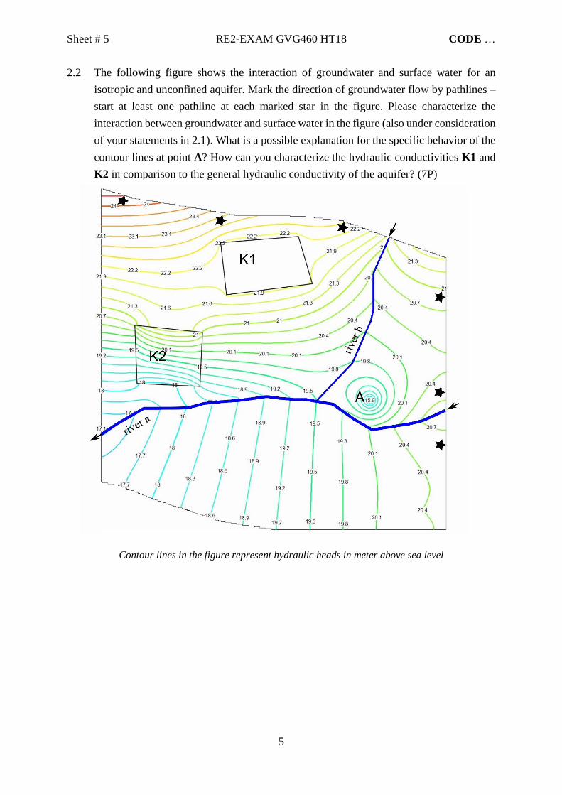
2.2 The following figure shows the interaction of groundwater and surface water for an

isotropic and unconfined aquifer. Mark the direction of groundwater flow by pathlines –

start at least one pathline at each marked star in the figure. Please characterize the

interaction between groundwater and surface water in the figure (also under consideration

of your statements in 2.1). What is a possible explanation for the specific behavior of the

contour lines at point A? How can you characterize the hydraulic conductivities K1 and

K2 in comparison to the general hydraulic conductivity of the aquifer? (7P)

Contour lines in the figure represent hydraulic heads in meter above sea level


6

2.3 Explain groundwater recharge! What is it? Why do we need to know it? Why is it difficult

to measure and to determine? Name and briefly describe two different methods that can

be used to determine the recharge to an unconfined aquifer. What data and information is

needed for either method? Use sketches. (6P)


7

3 Groundwater Flow and Aquifer Tests (total 27P)

3.1 Classify the following groundwater flow equation.

0 =𝜕

𝜕𝑥[𝑇(𝑥, 𝑦)

𝜕ℎ

𝜕𝑥] +

𝜕

𝜕𝑦[𝑇(𝑥, 𝑦)

𝜕ℎ

𝜕𝑦]

regarding

dimensionality of the flow domain,

heterogeneity / homogeneity,

isotropy / anisotropy,

steady-state / transient flow,

existence of sinks / sources

and explain and justify your answers. (5P)

3.2 What do the Dupuit assumptions state? Please explain with a suitable sketch. (3P)

3.3 Which additional aquifer property can we determine from a transient pumping test that

we cannot get from a steady state test? Why can we not get this property from a steady

state test? (3P)


8

3.4 A well in an unconfined aquifer is pumped at a rate of 0.012 m3/s until steady state is

reached. The saturated thickness of the aquifer prior to pumping was 15 m. At steady

state the drawdown s [m] in an observation well 20 m away from the pumping well is

0.26 m, the drawdown in an observation well 100 m away from the pumping well is 0.18

m. Drawdown s [m] indicates the difference between the initial water table elevation and

the water table elevation at steady state. What is the hydraulic conductivity [m/s] of the

aquifer? (5P)


9

3.5 A well in a confined aquifer is pumped at a rate of 25 l/s. The aquifer’s hydraulic

conductivity is 1.5*10-3 m/s. The aquifer thickness is 10 m. The storativity is 6.5*10-4.

The aquifer and the well fulfil the requirements to apply the Theis solution. Determine

the drawdown 26.12 m away from the well after 102 h of pumping (4P)


10

3.6 A well W1 is situated in proximity to impermeable material (e.g. bedrock). The situation

is shown in the figure below. You are asked to predict drawdown at the observation O1

as function of time. Please explain how you would solve this task under consideration of

the principle of superposition. Complete the side view part of the figure below (e.g. mark

the cone of depression etc.) and consider this for your explanation! (7P)


11

4 Groundwater Modelling (total 15P)

Numerical groundwater models are useful tools to manage aquifers. Think about a situation like

Varnum where a numerical model is requested to predict the impact of possible water

exploration on future conditions.

4.1 For what typical question or reason is a numerical groundwater model in a situation like

Varnum useful? Explain at least two. (2P)

4.2 Explain the general workflow for a numerical model that is intended to predict future

conditions. Start with “Identify Question / Define purpose”. (7P)


12

4.3 Explain with a sketch and words the three main types of boundary conditions. What

information / parameters are usually necessary to consider these boundaries within a

numerical model? (6P)


13

5 Groundwater Transport and Tracers, Contaminant Hydrogeology (total 10P)

5.1 Explain the terms: diffusion, dispersion, advection and retardation with respect to the

transport of solutes and particles in groundwater. (4P)


14

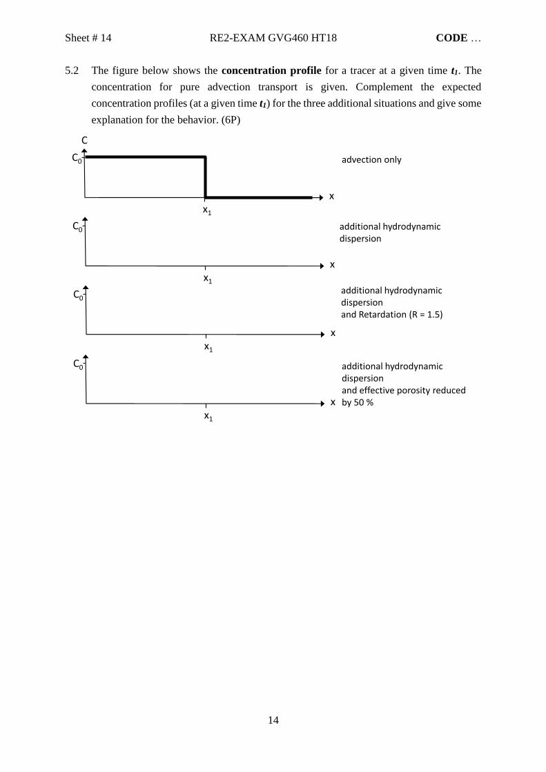
5.2 The figure below shows the concentration profile for a tracer at a given time t1. The

concentration for pure advection transport is given. Complement the expected

concentration profiles (at a given time t1) for the three additional situations and give some

explanation for the behavior. (6P)

C0

xx1

C0

xx1

C0

C

xx1

additional hydrodynamic dispersion

additional hydrodynamic dispersionand Retardation (R = 1.5)

C0

xx1

additional hydrodynamic dispersionand effective porosity reduced by 50 %

advection only


15

6 Fractured Rock Hydrogeology (total 6P)

6.1 How is the aperture of a fracture mathematically related to the volumetric flow rate

through this fracture? (3P)

6.2 What is a representative elementary volume (REV) and what relevance does this concept

have with respect to describing and modelling groundwater flow in a fractured system?

(3P)


16

Appendix 1 Equations

Theis’ equation, unsteady flow towards a well in a confined aquifer

where

s: drawdown [m]

Q: pumping rate [m3/s]

T: transmissivity [m2/s]

S: storativity [ ]

t: time [s]

W(u), u: well function and argument u, for tabulated values see Appendix 2

r: distance of the observation well to the pumping well [m]

Thiem’s equation for steady flow with two observation wells

𝑇 =𝑄

2𝜋(𝑠1−𝑠2)𝑙𝑛

𝑟2

𝑟1; for confined aquifers

𝐾 =𝑄

𝜋(𝑏22−𝑏1

2)ln

𝑟2

𝑟1; for unconfined aquifers

where:

s1: drawdown [m] in the observation well closer to the pumping well

s2: drawdown [m] in the observation well farther away from the pumping well

b1: saturated aquifer thickness [m] in the observation well closer to the pumping well

b2: saturated aquifer thickness [m] in the observation well farther away from the pumping

well

r1: distance to the pumping well [m] of the observation well closer to the pumping well

r2: distance to the pumping well [m] of the observation well farther away from the pumping

well



𝑠 =𝑄

4𝜋𝑇𝑊(𝑢) 𝑢 =

𝑟2𝑆

4𝑇𝑡


17

Cooper Jacob equations

1. Time Drawdown

2

025.2

r

TtS

2. Distance Drawdown

2

0

25.2

r

TtS

where:

s: drawdown difference between two observation wells [m] (to be determined!)

r: distance of the observation to the pumping well [m]

r0: distance of an observation well where the assumed drawdown is 0 [m] (to be determined!)

t: time after pumping started [s]

t0: time when the assumed drawdown is 0 [s] (to be determined!)



S: storativity [ ]

𝑇 =2.3𝑄

4𝜋(∆𝑠)

𝑇 =2.3𝑄

2𝜋(∆𝑠)


18

Appendix 2


19


20

re2-exam gvg460 applied hydrogeology - canvas

Documents