w a t e r r e s e a r c h 4 4 ( 2 0 1 0 ) 1 1 7 0 – 1 1 8 1

Avai lab le at www.sc iencedi rect .com

journa l homepage : www.e lsev i er . com/ loca te /wat res

Vulnerability of unconfined aquifers to virus contamination

J.F. Schijven a,*, S. Majid Hassanizadeh b, Ana Maria de Roda Husman c

a Expert Centre for Methodology and Information Services, National Institute of Public Health and the Environment (RIVM), P.O. Box 1, 3720

BA Bilthoven, The Netherlandsb Department of Earth Sciences, Utrecht University, P.O. Box 80021, 3508 TA Utrecht, The Netherlandsc Laboratory for Zoonoses and Environmental Microbiology, National Institute for Public Health and the Environment, P.O. Box 1, 3720 BA

Bilthoven, The Netherlands

a r t i c l e i n f o

Article history:

Received 27 April 2009

Received in revised form

24 September 2009

Accepted 6 January 2010

Available online 15 January 2010

Keywords:

Groundwater

Setback distance

Virus

Vulnerability

* Corresponding author. Tel.: þ31 302742994;E-mail addresses: jack.schijven@rivm.nl

rivm.nl (A.M. de Roda Husman).0043-1354/$ – see front matter ª 2010 Elsevidoi:10.1016/j.watres.2010.01.002

a b s t r a c t

An empirical formula was developed for determining the vulnerability of unconfined sandy

aquifers to virus contamination, expressed as a dimensionless setback distance r�s . The

formula can be used to calculate the setback distance required for the protection of

drinking water production wells against virus contamination. This empirical formula takes

into account the intrinsic properties of the virus and the unconfined sandy aquifer. Virus

removal is described by a rate coefficient that accounts for virus inactivation and attach-

ment to sand grains. The formula also includes pumping rate, saturated thickness of the

aquifer, depth of the screen of the pumping well, and anisotropy of the aquifer. This means

that it accounts also for dilution effects as well as horizontal and vertical virus transport.

Because the empirical model includes virus source concentration it can be used as an

integral part of a quantitative viral risk assessment.

ª 2010 Elsevier Ltd. All rights reserved.

1. Introduction Human pathogenic viruses, such as enterovirus, adeno-

The use of groundwater as a source for drinking water

production is often preferred because of its generally good

microbial quality in its natural state as compared with for

instance fresh surface water. Nevertheless, it may be readily

contaminated and outbreaks of disease from contaminated

groundwater sources are reported in countries at all levels of

economic development (Howard et al., 2006). The contribution

of groundwater to the global and significant incidence of

waterborne disease cannot be assessed easily because of

many competing transmission routes (Howard et al., 2006). In

this regard, viruses are considered to be the most critical

pathogens for groundwater contamination, because of their

ability to travel through the subsurface and their high infec-

tivity (Schijven and Hassanizadeh, 2000).

fax: þ31 302744434.(J.F. Schijven), hassaniza

er Ltd. All rights reserved

virus, norovirus, reovirus, rotavirus, and hepatitis A viruses,

have been detected in groundwater with molecular and/or cell

culture techniques with prevalence rates varying from 8% to

23% (Fout et al., 2003; Borchardt et al., 2003, 2007). Contami-

nation of drinking water from groundwater with human

pathogenic viruses may lead to epidemics that cause severe

illness and even death (Maurer and Sturchler, 2000; Par-

shionikar et al., 2003; Kim et al., 2005; Jean et al., 2006; Gallay

et al., 2006). Note that in cases of outbreaks and/or where high

prevalence rates of viruses in groundwater samples were

found, it often concerned vulnerable geologic settings.

Examples of such situations are fractured rock aquifers, cross-

connecting well bores, or leaking well cases in sandstone and

shale aquifers (Powell et al., 2003; Borchardt et al., 2007) in

combination with the presence of significant sources of

deh@geo.uu.nl (S.M. Hassanizadeh), ana.maria.de.roda.husman@

.

w a t e r r e s e a r c h 4 4 ( 2 0 1 0 ) 1 1 7 0 – 1 1 8 1 1171

contamination, such as wastewater treatment facilities,

septic tanks, and animal manure (Parshionikar et al., 2003;

Gallay et al., 2006; Jean et al., 2006; Fong et al., 2007).

Frost et al. (2002) stated that the occurrence of virus

contamination in groundwater may be overestimated,

because many studies selected high-risk wells for testing. At

four possibly vulnerable unconfined sandy aquifers in the

Netherlands, no viruses or bacteria were detected in large

volume samples, probably because potential fecal contami-

nation sources were too far away from the production wells

(Wuijts et al., 2008). Often, groundwater contamination occurs

as a peak event, hampering detection. Borchardt et al. (2003)

found that contamination was transient, since none of the

wells in their study was virus positive in two sequential

samples. In addition, when molecular detection is used for

virus enumeration, it is important to take into consideration

that the fraction of infectious virus is time and temperature

dependent (De Roda Husman et al., 2009). By using an opti-

mized cell culture-PCR assay for detection of rotavirus strains

in naturally contaminated source waters, Rutjes et al. (2009)

found that the broad variation observed in the ratios of rota-

virus RNA and infectious particles demonstrates the impor-

tance of detecting infectious viruses instead of viral RNA for

the purposes involving estimations of public health risks.

Given the difficulties in monitoring for and interpretation

of groundwater contamination, one should better aim at

preventing contamination. To prevent microbial contamina-

tion of groundwater, sources of contamination should be kept

at such a distance from the abstraction well that the produced

groundwater complies with a health-based target concen-

tration. Such a setback distance would allow for adequate

reduction of pathogen concentrations by means of natural

attenuation processes in the subsurface. This leads to the

definition of protection zones within which sources of faecal

contamination, such as sewers, septic tanks, and manure

depots are not allowed. For protection against pathogens,

usually a zone based on travel time is applied, and in several

countries this is a travel time of 50–60 days, e.g. in Austria,

Denmark, Germany, Ghana, Indonesia, UK (Chave et al., 2006).

Also, in the Netherlands protection of groundwater wells is

still based on the assumption that a travel time of 60 days is

sufficient for die-off of pathogenic bacteria in contaminated

groundwater to the extent that no health risks would exist

(CBW, 1980). However, it is known that pathogenic viruses and

protozoa as well as bacteria can survive much longer than 60

days in soil and groundwater (Pedley et al., 2006). Given the

persistence of pathogens, a protection zone of 60 days may

not be sufficient to protect public health.

In the third edition of World Health Organization’s Guide-

lines, a preventive management framework for safe drinking

water is outlined that entails health-based targets, water

safety plans and surveillance (WHO, 2008). Based on these

guidelines, Dutch legislation for drinking water has imple-

mented as microbiological health-based target that patho-

genic microorganisms in drinking water may not exceed

a limit associated with a risk of infection of one per ten

thousand persons per year (VROM, 2001; De Roda Husman and

Medema, 2005). This raises the question whether a 60-day

groundwater protection zone is an adequate barrier to safe-

guard this risk level.

Dutch drinking water legislation requires that compliance

of drinking water with the maximum risk of infection of one

per ten thousand persons per year to be demonstrated by

means of a Quantitative Microbiological Risk Assessment

(QMRA). This QMRA should be conducted for drinking water

that is produced from surface water and also for groundwater

from vulnerable groundwater well systems (VROM, 2001).

According to the Dutch Environmental Inspectorate Guideline

(DEIG), all unconfined aquifers are considered to be vulnerable

(De Roda Husman and Medema, 2005). However, groundwater

companies have argued that deep unconfined aquifers with

the top of the well screen at a significant depth, should not be

considered vulnerable. This is a sensible argument, but an

objective distinction between deep and shallow has not been

made (Schijven and de Roda Husman, 2009).

In order to address some of these questions, Schijven et al.

(2006) simulated a situation where a sewer was continuously

leaking viruses at the groundwater table. Processes that

attenuate virus concentration were assumed to be virus inac-

tivation, attachment of virus particles to the sand grains, and

dilution. Steady-state one-dimensional flow and transport

was assumed and parameter uncertainties were included.

Protection zones were calculated for shallow unconfined

aquifers using a stochastic steady-state model. Using litera-

ture data for virus inactivation in groundwater (from Pedley

et al., 2006) and a conservative estimate of the attachment rate

coefficient (from Schijven et al., 2000), Schijven et al. (2006)

calculated protection zones for shallow unconfined sandy

aquifers that would allow protection against virus contami-

nation to the level that the infection risk of one per 10 000

persons per year is not exceeded with a 95% certainty. In those

cases, instead of 60 days, one to two years of travel time were

needed, corresponding to setback distances of about

200–400 m. As only horizontal transport was considered in that

study, effects of vertical transport, confining layers and vadose

zone were not modelled. In the case of deeper abstraction,

vertical transport should be taken into account as otherwise

the protection zone size will be overestimated.

The concept of groundwater vulnerability does not have any

objective and standardized definition in literature, despite

numerous works on this topic (Sinan and Razack, 2009). Sinan

and Razack (2009) have given a brief review of a number of

models for assessing intrinsic groundwater vulnerability.

Amongst others, these models include DRASTIC, GOD, SIN-

TACS, CALOD and EPIK. The majority of these models use

relative ranking schemes to calculate a vulnerability index. To

our understanding, such relative ranking, which is, for

example, also a common approach in risk assessment using

Failure Mode and Effect Analysis (FMEA), is rather arbitrary,

because it serves to accomplish ranking, but its actual value

cannot be considered to be a good quantitative measure. An

index value that is twice as high does not necessarily mean

risks are twice as high too. Instead, in the present paper, we

have chosen to develop a quantitative vulnerability index that

can be used to determine setback distance to specifically

protect against virus contamination, that can be used to

prioritize aquifers according to vulnerability, and that can be

part of QMRA. Here, we have adopted the definition of vulner-

ability given by Vbra and Zaporozec (1994): Vulnerability

comprises those intrinsic properties of the strata separating

w a t e r r e s e a r c h 4 4 ( 2 0 1 0 ) 1 1 7 0 – 1 1 8 11172

a saturated aquifer from the land surface which determine the

sensitivity of that aquifer to being adversely affected by pollu-

tion loads applied at the land surface. Note that a vulnerable

aquifer is only at risk if a contamination source is present.

Advection, dispersion and dilution of viruses are deter-

mined by the pumping rate of the abstraction well, the leakage

rate of the contaminating source, the hydraulic conductivities

of the aquifer layers, and the aquifer thickness. Virus attach-

ment and inactivation depend on the type of virus as well as

physico-chemical properties of the water and soil grain

surfaces (Schijven and Hassanizadeh, 2000). Straining may

come into play as well, especially in the presence of manure or

wastewater, which have high contents of suspended solids

(Bradford et al., 2006a).

In the present study, a formula is developed for simulating

the transport of viruses from a contamination source at or

near the land surface to a groundwater abstraction well.

Effects of vertical flow and transport are taken into account.

The model is used to develop an empirical formula for the

evaluation of the vulnerability of unconfined aquifers to virus

contamination, based on intrinsic aquifer and virus properties

as well as hydraulic parameters.

One may question the utility ofa simple algebraic formula for

the determination of setback distances, given the fact that

powerful multidimensional groundwater models can be set up

for each and every groundwater production site. But, such

models are only valuable if detailed information about intrinsic

properties of the aquifer and viruses exist. Based on our expe-

rienceofexploringavailabledataonaquifers intheNetherlands,

often such data are unavailable. We suspect that in larger

countries, with a greater variety in geologic settings and many

(small) groundwater production systems, information on

vulnerability characteristics is sparse too. A quick and easy-to-

use formula can serve to identify vulnerable aquifers and situ-

ations that require additional attention. These cases can be then

considered for detailed investigation and comprehensive

modelling.

Parameters in the virus transport model that represent

intrinsic properties determining aquifer vulnerability, may

work together or counteract. This could complicate definition

of vulnerability and may also introduce too much detail in

such a definition. Therefore, a virus transport model with

a limited number of dimensionless parameters was set up to

evaluate the combined effect of parameters. This dimen-

sionless model produces a dimensionless setback distance, r�s ,

that is required for adequate groundwater protection.

This dimensionless setback distance is a measure of

vulnerability, because it is proportionate to the required virus

reduction. By back transformation, the actual setback

distance can be found for a given aquifer. To our knowledge,

such a quantitative vulnerability index for groundwater to

virus contamination does not exist.

2. Dimensionless model

The typical system considered here for the calculation of the

extent of the protection zone is an unconfined aquifer wherein

a single well or a closely-spaced cluster of production wells is

operating. Further, the presence of a source situated at the

groundwater table at a certain distance from the abstraction

well was considered. The source was assumed to be leaking

continuously at a constant rate, containing a constant

concentration of viruses. The leakage is assumed to have been

going on for some time and the well is operating at a constant

average production rate. Therefore, steady-state conditions

may be assumed. Assuming that the aquifer consists of

homogeneous horizontal layers, the flow can be considered to

be axisymmetrical. The governing equation for the radial

water flow under steady-state conditions is as follows:

kzv2hvz2þ kr

rv

vrrvhvr¼ 0 (1)

where, t [T] is the time and, h [L] is the hydraulic head. In order

to simplify the model, it was assumed that all aquifer layers

are combined into a single layer with total thickness H [L] and

effective vertical and horizontal permeabilities kz [LT�1] and kr

[LT�1].

Division of equation (1) by kr and scaling to H leads to the

following dimensionless flow equation:

1m

v2h�

vz�2þ 1

r�v

vr�

�r�

vh�

vr�

�¼ 0 (2)

where m is the anisotropy factor kr=kz, which is expected to be

a relevant factor for evaluating vertical transport relative to

horizontal transport. All dimensionless parameters in equa-

tion (2) are indicated with a superscript asterisk, except for m.

These dimensionless parameters and their definitions are

listed in Table 1.

Even though the water flow is radially symmetric, the virus

transport is not because the leakage was considered to occur

at a single point. However, if dispersion tangential to the flow

is neglected, transport may also be modelled as radially

symmetric and steady-state. It was then assumed that the

leakage was spread over a ring around the abstraction well.

The governing virus transport equation is given by:

vzvCvzþ vr

vCvr� Dzz

v2Cvz2� 1

rv

vr

�Drrr

vCvr

�¼ �lC (3)

where, vz ¼ ð�kz=nÞðvh=vzÞ and vr ¼ ð�kr=nÞðvh=vrÞ are the

vertical and radial pore water velocities, respectively, with

porosity denoted by n. l [T�1] is the virus removal rate coeffi-

cient, which entails both attachment and inactivation. From

breakthrough curves obtained in field studies on virus trans-

port, it has become clear that attachment and inactivation are

the major removal processes. Virus detachment, commonly

takes place at a much slower rate and its effect on virus

concentration under steady-state conditions may be neglected

(Schijven et al., 1999, 2000). Commonly, virus inactivation is

considered to proceed as a first order rate process (Pedley et al.,

2006), although observations over long periods of one to two

years demonstrate the existence of very persistent virus

subpopulations (De Roda Husman et al., 2009; Meschke, 2001).

Virus attachment may be described using colloid filtration

theory (e.g. Tufenkji and Elimelech, 2004), whereby intrinsic

properties of virus, such as size and electric charge, and of the

porous medium, such as pH, ionic strength and grain size, come

into play. The current study is focussed on the hydrologic

Table 1 – Dimensionless parameters, all denoted witha superscript*, except for m.

Parameter Description

A�s ¼ 2r�s ls Leakage area

A�w ¼Aw

pH2Cross-sectional area of the screen of the

abstraction well

a�r ¼ arH ¼ 0:005r�s Dispersivity in the r-direction.

a�z ¼ azH ¼ 0:1a�r Dispersivity in the z-direction

C� ¼ CCR

Virus concentration with CR [L�3] the

concentration at the abstraction

well at R [L] from the source of

contamination.

C�s Virus concentration at the contamination

source

h� ¼ hH Hydraulic head

k�r ¼ krpH2

Q ¼ pHQ

Ptri Horizontal hydraulic conductivity, where

tri [m2 day�1] is the transmissivity of i-th

aquifer layer.

l� ¼ lnpH3

Q Dimensionless removal rate coefficient,

m ¼ krkz

Anisotropy ratio, where

kz ¼ ðHþ HdÞ=ðP

Hi=P

kz;iÞ þP

rd;i and Hd

[m] is the total thickness of all aquitards,

Ht [m] is the thickness of the i-th aquifer

layer, and kz,i [m day�1] is the hydraulic

conductivity in the vertical direction of

the i-th aquifer layer. Because no data for

kz,i were available, the values of kz,i were

taken. Finally, rd,i[day] is the resistivity of

the i-th aquitard. Note that only the

aquitards between to aquifers that were

penetrated by the screen of the well were

considered.

Q� ¼ qQ Dilution, where q ¼ 1 m3 day�1 (Schijven

et al., 2006).

r� ¼ rH; z� ¼ z

H Radial and vertical coordinate

v�r ¼ npH2

Q vr; v�z ¼ npH2

Q vz Radial and vertical pore water velocity

z�b ¼ 1� zbH ; z�t ¼ 1� zt

H Bottom and top of the well screen

(r1*,z1

*) (r2*,z1

*)

(r2*,z2

*)(r1*,z2

*)

(r1*,zt

*)

(r1*,zb

*)

(rs*,z2

*) (rs*+ls,z2

*)

BC0

BC0 BC0

BC0

BC1

BC2

BC3

BC0

H/H=1

Q*

rs

*=r

s/H Virus source

Well screen

Fig. 1 – Cross-section of axisymmetrical dimensionless

modelling domain with r- and z-coordinates and boundary

conditions BC0 (no flux of water or virus), BC1 (water enter

the domain), BC2 (water and virus enter the domain) and

BC3 (water and virus leave the domain at the well). r�s is the

dimensionless setback distance and vulnerability index.

Corresponding boundary condition equations for water

flow and virus transport are listed in Table 2. Gray lines:

Direction of water flow. Dotted lines: Direction of water and

virus inflow.

w a t e r r e s e a r c h 4 4 ( 2 0 1 0 ) 1 1 7 0 – 1 1 8 1 1173

properties of the aquifer. But, the empirical formula that is

being developed can always be extended with the intrinsic

properties of virus and porous medium that determine their

interaction.

Dzz and Drr [L2T�1] are the dispersion coefficients in z and r

directions, given by:

Dzz ¼ azjvj þ Ddiff þ ðar � azÞvzvz

jvj (4)

Drr ¼ azjvj þ Ddiff þ ðar � azÞvrvr

jvj (5)

where az and ar [L] are the vertical and radial dispersivities, jvj[LT�1] is the velocity magnitude and Ddiff [L2T�1] is the

molecular diffusion coefficient. The latter was neglected in

the calculations. It is assumed that az ¼ 0:1ar.

The corresponding dimensionless virus transport equation

is as follows:

v�zvC�

vz�þ v�r

vC�

vr�� 0:1a�r v

�r

v2C�

vz�2� 1

r�a�r

v

vr�

�v�r r

�vC�

vr�

�¼ �l�C� (6)

See Table 1 for the definition and listing of all dimensionless

parameters.

3. Dimensionless domain and boundaryconditions

In Fig. 1, the axisymmetrical dimensionless modelling domain

is shown, where the dimensionless setback distance r�s ¼ rs=H

is also shown. This is the vulnerability index, which allows to

compare aquifers according to their vulnerability. Aquifers

with the same r�s are equally vulnerable, i.e. in those aquifers,

viruses are reduced in concentrations to the same extent.

Aquifers with the same r�s may have different setback

distances, if they differ in saturated thickness.

All water flow and virus transport boundary conditions are

listed in Table 2. At boundary BC1 between ðr�2; z�1Þ and ðr�2; z�2Þwhere water enters the domain, it is assumed that the

hydraulic head h* is a given constant (in these simulations,

equal to the saturated aquifer thickness, i.e. h*¼ 1), but there is

no virus entering, so the total virus flux is zero.

At boundary BC2 between ðr�s ; z�2Þ and ðr�s þ ls; z�2Þ a line

source with thickness ls is situated at the water table where

there is a continuous flux of virus and flux of wastewater into

the domain. Note that the concentration of virus entering the

domain from the point source is actually averaged over an

entire ring. This allows us to assume axisymmetric flow and

transport. This assumption implies that tangential dispersion

is insignificant. This also accounts for the fact that the

concentration of viruses arriving at the well will be diluted by

clean water entering the well from other directions.

At boundary BC3, between ðr�1; z�bÞ and ðr�1; z�t Þ, the screen of

the abstraction well is situated where there is flux of water

and virus out of the domain.

BC0 between ðr�1; z�1Þ and ðr�2; z�1Þ, between ðr�s þ ls; z�2Þ and

ðr�s ; z�2Þ, between ðr�1; z�2Þ and ðr�s ; z�2Þ, between ðr�1; z�2Þ and ðr�1; z�t Þ,and between ðr�1; z�1Þ and ðr�1; z�bÞ, designates no flux of water

and no flux of viruses across the boundaries.

In all simulations, the size of the modelling domain was

kept constant, i.e. the saturated aquifer thickness of the

Table 2 – Boundary conditions (see Fig. 1 for schematic of modelling domain).

Boundary Description Water flow Virus transport

BC0 No flux of water and no flux

of virus across boundary

vh�

vr� ¼ 0 vC�

vr� ¼ 0

BC1 Right outer boundary: Water enters,

constant head, no virus flux

h* ¼ 1 �a�r v�rvC�

vr� ¼ �v�r C�

BC2 Line source of virus at water table

with constant flux of wastewater

and virus into the domain

vh�

vz� ¼ �Q�

A�s k�z�0:1a�r v�r

vC�

vz� ¼ �Q�

A�sC�s � v�zC�

BC3 Screen of abstraction well with

constant flux of water and virus

out of the domain

vh�

vr� ¼ � 1A�wk�r

vC�

vr� ¼ 0

w a t e r r e s e a r c h 4 4 ( 2 0 1 0 ) 1 1 7 0 – 1 1 8 11174

domain was one and the radius was 50. Thus, r�1 ¼ 0:001,

r�2 ¼ 50, z�1 ¼ 0, z�2 ¼ 1, ls ¼ 0.01.

Table 4 – Simulated cases. N [ 212. l* was varied from0.01 to 1000.

C�s Q* m z�t z�b

1 4 0.001 1 1 0.50

2 5 0.001 1 1 0.50

3 6 0.001 1 1 0.50

4 7 0.001 1 1 0.50

5 8 0.001 1 1 0.50

6 8 0.001 1 1 0.75

7 8 0.001 2 1 0.50

8 8 0.001 5 1 0.50

9 8 0.001 10 1 0.50

10 8 0.0001 1 1 0.50

11 8 0.0001 2 1 0.50

12 9 0.001 1 1 0.50

13 4 0.001 1 0.50 0

14 5 0.001 1 0.50 0

15 6 0.001 1 0.50 0

16 7 0.001 1 0.50 0

17 8 0.001 1 0.25 0

4. Implementation into FlexPDE code anddefinition of cases

The dimensionless flow equation (2) and the dimensionless

virus transport equation (6) were solved using FlexPDE (2004,

version 4.1, PDESolutions Inc, Cambridge MA, USA). FlexPDE is

a script-driven program. It reads a description of the equa-

tions, domain, auxiliary definitions and graphical output

requests from a text file. The FlexPDE problem descriptor

language can be viewed as a shorthand language for creating

finite element models.

The Dutch groundwater database LGM at the National

Institute of Public Health and the Environment in the

Netherlands contains hydrologic data from most unconfined

(137 sites) and semi-confined (87 sites) aquifers in the

Netherlands, which are in use for drinking water production

(Kovar et al., 2005). Of those, 35 unconfined aquifers could be

selected of which all required hydrologic data were present to

compile the values of dimensionless parameters.

Schijven et al. (2006) chose the value for attachment and

inactivation based on literature data, where the mean value

for inactivation represented relatively stable viruses at

a temperature of about 10 �C and where the attachment value

was a conservative estimate from a field study. The resultant

of those processes gives an approximate value of 0.03 day�1

for l. This value was used as a default value of l. For porosity n

a default value of 0.35 was used. For dispersivity a�R, the value

of 0:005r�s was employed. The justification for this assumption

Table 3 – Values of dimensionless parameters andaquifer thickness H from 35 unconfined aquifers.

Dimensionless parameter Mean Min Max

l* 45 0.079 645

Q* 0.00012 0.000037 0.0019

k�r 500 4.4 6900

m 1.6 1 3.5

z�t 0.72 0.31 1

z�t � z�b 0.43 0.042 0.82

H (m) 116 23 334

comes from dispersivity values that were found in two field

studies in the Netherlands (Schijven et al., 1999, 2000).

The aquifers in the LGM database are schematisized into

four layers of aquifers and three aquitards between two

subsequent layers of aquifers. Values of transmissivity for

aquifers and values of resistivity for aquitards are available

from the database. In addition, the database contains data on

the depths of these layers, the depth of the top and bottom of

the filter screen of the production well and its pumping rate.

From these data the values of dimensionless parameters l*,

Q*, k�r , m, z�t , and z�b were calculated. Table 3 summarizes the

18 8 0.001 1 0.50 0

19 8 0.001 1 0.50 0.25

20 8 0.001 1 0.75 0.25

21 8 0.001 1 0.75 0.50

22 8 0.001 1 0.85 0.35

23 8 0.001 1 0.85 0.60

24 8 0.001 1 0.50 0

25 8 0.001 1 0.50 0

26 8 0.001 2 0.50 0

27 8 0.001 5 0.50 0

28 8 0.001 10 0.50 0

29 8 0.0001 1 0.50 0

30 8 0.0001 2 0.50 0

31 8 0.0001 5 0.50 0

32 8 0.0001 10 0.50 0

w a t e r r e s e a r c h 4 4 ( 2 0 1 0 ) 1 1 7 0 – 1 1 8 1 1175

mean, minimum and maximum values of these dimension-

less parameters. These values were taken as the basis for

defining a large number of cases for numerical simulation.

These cases are listed in Table 4. These cases were simulated

with values for l* varied between 0.01 and 1000.

Assuming that the virus concentration at the point of

leakage is in the order of one hundred virus particles per litre

(Schijven et al., 2006), virus concentrations need to be reduced

by a factor of 108 from the contamination source to the well.

Thus, by setting C�s ¼ 108, C* at the well should be equal to one,

corresponding to an actual virus concentration at the well of

CR ¼ 10�6 virus particles per litre. Therefore, most cases were

run with C�s ¼ 108. In addition, in order to evaluate the relation

of virus source concentration reduction and setback distance,

series of cases were simulated with C�s ¼ 104;105;106;107;109.

When running FlexPDE for a particular case, a value for C*

at the pumping well is the model result. By manually

adjusting r�s and running FlexPDE again, a value for r�s was

sought such that C*¼ 1� 0.05. The margin of 0.05 was allowed

in order to limit the number of runs needed to find a r�s value.

From the numerical simulations, r�s values were obtained

for the defined cases as well as for selected unconfined

aquifers.

An empirical formula was developed by fitting r�s values as

a function of dimensionless parameters l*, Q*, k�r , m, z�t , and z�busing Mathematica (version 7, Wolfram Inc.). Several empir-

ical formulas were evaluated, consisting of terms of products

of coefficients and the model parameters. Some model

parameters were log-transformed. Using non-linear model

fitting, values for the coefficients were estimated. This

kj

a b

ed

g h

Fig. 2 – Results from numerical calculations (points) an

command also provides P-values (c2-statistic) and R2-values.

An empirical formula was considered to be acceptable if the P-

values were less than 0.1%. The formula with the highest R2-

value was chosen as the best model.

5. Results and empirical model development

A series of simulations with C�s ¼ 108, Q* ¼ 0.001, m ¼ 1,

z�t � z�b ¼ 0:5 and a range of values for z�t , k�r and l* (see Table 3)

was conducted to generate r�s values that were needed for the

development of the empirical formula.

In doing so, it appeared that there was no effect of k�r on the

value of r�s . Consequently, the value of k�r was set equal to 100

in all other simulations and k�r was not included in the

development of the empirical formula for r�s .

Figs. 2 and 3 show the graphs of all simulated cases

together with the fitted model. For the fitting procedure,

a two-step approach was followed. Fig. 2 shows that if

z�t ¼ 1; lnr�s appears to be linearly related with ln l*. Therefore,

a power law model was fitted first to these cases. Clearly, l* is

the dominating factor in determining r�s . If l* increases, r�sdecreases strongly, i.e. the aquifer would be less vulnerable.

If z�t ¼ 1, virus transport to the well will be mainly hori-

zontal and r�s can also be approximated by the following

simple steady-state solution of equation (6), where dispersion

has been neglected:

r�s ¼�ln�C�sQ

���0:5l��0:5 (7)

i

c

f

l

d fitted formula (line) for those cases where z�t [1.

w a t e r r e s e a r c h 4 4 ( 2 0 1 0 ) 1 1 7 0 – 1 1 8 11176

Note that although in equation (7) dispersion is neglected, it

is neglected neither in the numerical calculations with

FlexPDE nor in the development of the empirical model. Since

it was assumed that a�R ¼ 0:005r�s , a�R does not appear in the

empirical formula anymore and is hidden in the values of the

constants of the formula. Equation (7) only serves as

a conceptual starting point to develop a formula for the case

where z�t ¼ 1.

So, for our fitted formula, we sought a relationship similar

to (7). First, for z�t ¼ 1, corresponding data were fitted to the

following equation:

r�s ¼�ln�C�sQ

���a1l�a2 (8)

a

d e

b

nm

g h

j k

p q

Fig. 3 – Results from numerical calculations (points) an

This resulted in an excellent fit of the data, with a1 ¼ 0.557,

a2 ¼ �0.467 and R2 ¼ 99.9% (Table 5). Given the fact that these

values of a1 and a2 are near 0.5 suggests that, on the one hand,

equation (7) is a reasonable approximation for horizontal virus

transport and that, on the other hand, the numerical simu-

lations for z�t ¼ 1 make sense.

Including terms related to the other dimensionless

parameter to the formula showed no significant improved to

fitting the data. Interactions of the dimensionless parameters

did not contribute much either.

Fig. 3 shows that if z�t < 1; lnr�s declines rapidly for larger

values of ln l*. In those cases, vertical transport plays a more

significant role, therefore z�b and z�t come into play. Attempts

c

f

i

l

o

r

d fitted formula (line) for those cases where z�t <1.

Fig. 4 – Effect of z�t and Q*. If then the relation between ln l*

and lnr�s is linear. A smaller value of z�t results in a stronger

decline of lnr�s with at large ln l*. A smaller value of Q�

results in a smaller value for lnr�s.

w a t e r r e s e a r c h 4 4 ( 2 0 1 0 ) 1 1 7 0 – 1 1 8 1 1177

to fit a formula to all the data at once were successful,

however in the two-step approach better fitting was obtained

by using the first power law formula and extending it with an

exponential factor to account for the rapid decline of lnr�s for

high values of ln l*.

The combination of factors in the exponent that was found

gave the highest R2-value with P-values for the coefficients

less than 0.1%. Thus, a high R2-value of 97,9% was also

obtained when fitting all r�s-values, resulting in the following

empirical formula if z�t � 1

r�s ¼�lnC�sQ

��a1l�a2 Exp

hC�a3

s Q�a4 l�a5�a6z�t ma7 a8

�1� z�t

�Exp

�a9z�t � a10z�b

�i

(9)

Table 5 also lists the estimates of coefficients a3 . a10.

Figs. 4–7 are given to show the behavior of the model, i.e. to

demonstrate the effects of the dimensionless parameters.

Fig. 4 demonstrates the combined effect of z�t and Q*. If z�t ¼ 1

then the relation between ln l* and lnr�s is linear. A smaller

value of z�t results in a stronger decline of lnr�s at the larger

values of ln l*, but not for the smaller value of ln l* in the left

linear part of the curves. Apparently, a deeper filter screen in

the dimensionless domain (z�t < 1) makes an aquifer much less

vulnerable for the higher values of ln l*. In the model equation

this effect is implemented by the term with z�t only in the

exponential term of the model. The effect of z�t at large values of

ln l* is relatively strongest as indicated by the fact that coeffi-

cient a9 in the model (Table 5) has a relatively large value.

A smaller value of Q*, more dilution, results in a smaller value

for lnr�s , but in the dimensionless domain a ten times decrease

of Q* has only a small effect on lnr�s , especially if ln l* is small.

Next, Fig. 5 shows that smaller value of z�t � z�b results in

a higher value of lnr�s only if ln l* is large and for z�t < 1. Fig. 6

shows that if z�t ¼ 1 the value m has no effect, but if z�t < 1,

a higher value m results in a lower value of lnr�s at higher lnl�

where vertical transport becomes increasingly significant.

Note that in the case of (semi)confined sandy aquifers, the

value of m as calculated from kr and kz has a very large value.

In the case of z�t < 1 and m > 10, the empirical formula

(Equation (9)) predicts very small r�s values, or in other words, it

Table 5 – Values for Parameter coefficients a1 . a11 ofempirical formulas (equations (10) and (11)).

Coefficient Estimate Standard error

z�t ¼ 1 (equation (10))

a1 0.557 0.00363

a2 �0.467 0.00195

R2 ¼ 99.9%

z�t � 1 (equation (11))

a3 �0.227 0.0107

a4 �0.383 0.0212

a5 2.19 0.112

a6 1.17 0.133

a7 1.64 0.0578

a8 0.207 0.0593

a9 0.529 0.226

a10 2.99 0.240

R2 ¼ 97,9%

predicts confined aquifers are not vulnerable. This was also

found by means of numerical simulation using FlexPDE (data

not shown).

6. Discussion

An empirical formula was developed by fitting the results

from numerical calculations of r�s for various combinations of

l*, Q*, k�r , m, z�t , and z�b, all in a dimensionless domain. Using

this empirical model, one now can easily calculate rs ¼ r�sH for

a given aquifer. In this regard, dimensionless parameters l*,

Q*, m, z�t , and z�b are vulnerability parameters determining

vulnerability of the aquifer, where vulnerability is given by the

value of r�s . It was found that the value of k�r did not affect the

value of r�s .

Of the vulnerability parameters, l* is dominant. An

increase of l* leads to a decrease of r�s . A decrease of Q*, more

dilution, leads to a decrease of r�s , but this effect is partly

compensated by a shorter travel time. The value of m on r�s is

negligible if only horizontal transport is important. An

Fig. 5 – Effect of z�t Lz�b. A smaller value of z�t Lz�b results in

a higher value of lnr�s only at large ln l* and z�t <1.

Fig. 6 – Effect of m. If z�t [1, a higher value m results in

a slightly higher value of lnr�s. If z�t <1, a higher value m

results in a lower value of lnr�s at higher ln l*.

w a t e r r e s e a r c h 4 4 ( 2 0 1 0 ) 1 1 7 0 – 1 1 8 11178

increase of m leads to a decrease of r�s if vertical transport is

significant, because under those conditions vertical transport

is slower than horizontal transport. A decrease of z�t implies

that the screen of the well lies deeper. As a result, vertical

transport becomes more important, lowering r�s .

A decrease of the length of the screen of the pumping well,

z�t � z�b, only in the cases where vertical transport is significant,

increases r�s .

Instead of calculating the values of the dimensionless

parameters, in order to use the dimensionless empirical

model, one can also use the empirical formula that is trans-

lated to the dimensional form. The dimensional empirical

formula can be derived from the dimensionless formula by

substitution of the dimensionless parameters with the

dimensional parameters (Table 1):

rs ¼

0:96H�0:4

�ln

CC0� ln

Qq

�0:56

l�0:47Q0:47�

Exp

2664

0:25�

ztH � 1

�H6:6�3:5

ztH l2:2�1:2

ztH Q1:2ðzt

H�2:2m1:6�

Exp�� 0:23ln

CC0þ 0:38ln

Qqþ 0:43

zt

H� 3:0

zb

H

�3775

(10)

Fig. 7 – Effect of C�s. If z�t [1, a higher value m results in

a slightly higher value of lnr�s. If z�t <1, a higher value m

results in a lower value of lnr�s at higher ln l*.

Using equation (10) to calculate rs for a particular unconfined

sandy aquifer, one needs to have the values of the saturated

aquifer thickness H, the abstraction rate Q, depths of top and

bottom the well screen zt and zb, virus leakage rate q (default

value 1 m3 day�1), virus removal C=C0 (default value 108), and

removal rate coefficient l (default value 0.03 day�1). Note that

the default values given for the latter three parameters are

based on the assumptions given by Schijven et al. (2006). These

may be changed if other information on the virus source is

present and the desired target value for virus removal, which

may be based on a health target level. Also, if actual informa-

tion is available on virus inactivation and attachment for that

particular site, other values for l may be employed. For

example, one may also decide to apply a more (or less)

conservative approach.

If, on the one hand, the calculated value of rs happens to

exceed the actual setback distance, one may conclude that

additional safety measures, such as enlargement of the

protection zone or additional water treatment, are needed,

and/or one may decide to subject the aquifer to further inves-

tigation in order to obtain site-specific data for virus removal. If,

on the other hand, rs is smaller than the actual setback distance

one may conclude that the aquifer is adequately protected.

The abovementioned approach was applied to plot the

setback distances rs of the 35 selected unconfined sandy aqui-

fers from the LGM database in relation to their aquifer depth H

and to demonstrate the interplay of Q, H, zt and m (Fig. 8). In

Fig. 8, the solid lines correspond to two values for Q and

z�t ¼ zt=H ¼ 1, i.e. only horizontal transport is considered. The

dotted lines correspond to two values for Q and z�t ¼ zt=H ¼ 0:72,

which is the mean z�t of the 35 aquifers. The aquifers are denoted

with symbols and classified according to Q and z�t .

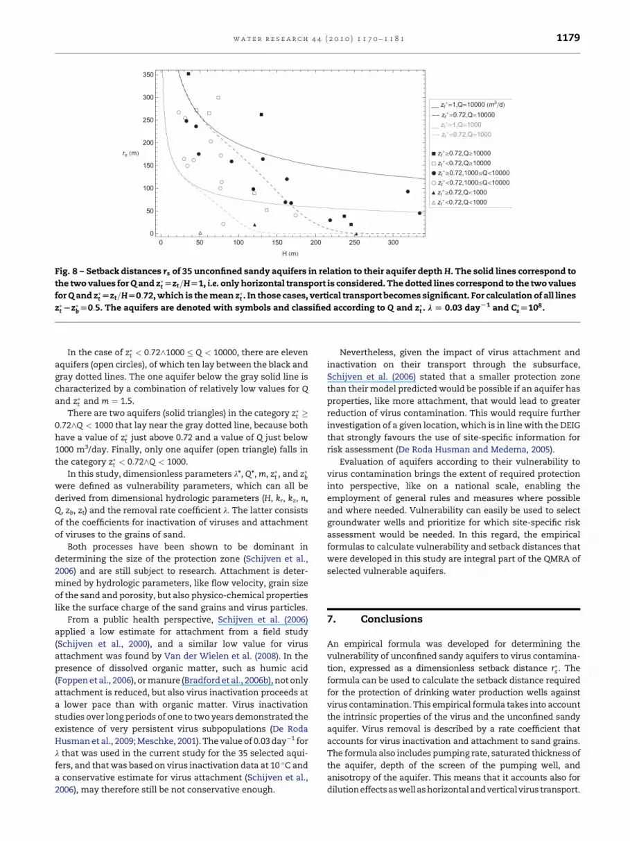
Fig. 8 shows that an increase in Q leads to an increase in rs,

despite more dilution of virus due to the increase of Q. Fig. 8

also demonstrates that for a given Q, the value of rs decreases

with H, but for larger H this effect is small. However, if the

screen of the well is deeper, then there is a strong reduction in

the required rs. This also demonstrates that deeper uncon-

fined aquifers with a deep well screen are substantially less

vulnerable. This not only confirms the opinion of Dutch

groundwater companies that deeper aquifers with a deeper

screen are less vulnerable, the empirical formula that was

developed in this study also provides a tool to actually

calculate vulnerability and the associated setback distance.

In the case of z�t � 0:72^Q � 10000, there are four aquifers

(solid squares), all with a high Q. The two left ones in Fig. 8

have a z�t of almost one and are relatively shallow, whereas

the two on the right side have a z�t just over 0.72 and are

relatively deep, therefore z�t is deep, hence the low setback

distance.

In the case of z�t < 0:72^Q � 10000, there are five aquifers

(open squares), of which four lay near the dotted line where

z�t ¼ 0:72^Q ¼ 10000. A lower value of z�t as well as a lower Q

results in a lower rs. In the case of the third aquifer from the left

in this category, Q is very high, hence the high position in Fig. 8.

In the case of z�t � 0:72^1000 � Q < 10000, there are twelve

aquifers (solid circles), of which eleven lay between the black

and gray solid lines. The one aquifer below the gray solid line

is characterized by z�t ¼ 0:77 in combination with a large H,

therefore zt lies deep.

rs

zt m

zt

zt

zt

zt

zt

zt

zt

zt

zt

Fig. 8 – Setback distances rs of 35 unconfined sandy aquifers in relation to their aquifer depth H. The solid lines correspond to

the two values for Q and z�t [zt=H[1, i.e. only horizontal transport is considered. The dotted lines correspond to the two values

for Q and z�t [zt=H[0:72, which is the mean z�t . In those cases, vertical transport becomes significant. For calculation of all lines

z�t Lz�b[0:5. The aquifers are denoted with symbols and classified according to Q and z�t . l [ 0.03 dayL1 and C�s[108.

w a t e r r e s e a r c h 4 4 ( 2 0 1 0 ) 1 1 7 0 – 1 1 8 1 1179

In the case of z�t < 0:72^1000 � Q < 10000, there are eleven

aquifers (open circles), of which ten lay between the black and

gray dotted lines. The one aquifer below the gray solid line is

characterized by a combination of relatively low values for Q

and z�t and m ¼ 1.5.

There are two aquifers (solid triangles) in the category z�t �0:72^Q < 1000 that lay near the gray dotted line, because both

have a value of z�t just above 0.72 and a value of Q just below

1000 m3/day. Finally, only one aquifer (open triangle) falls in

the category z�t < 0:72^Q < 1000.

In this study, dimensionless parameters l*, Q*, m, z�t , and z�bwere defined as vulnerability parameters, which can all be

derived from dimensional hydrologic parameters (H, kr, kz, n,

Q, zb, zt) and the removal rate coefficient l. The latter consists

of the coefficients for inactivation of viruses and attachment

of viruses to the grains of sand.

Both processes have been shown to be dominant in

determining the size of the protection zone (Schijven et al.,

2006) and are still subject to research. Attachment is deter-

mined by hydrologic parameters, like flow velocity, grain size

of the sand and porosity, but also physico-chemical properties

like the surface charge of the sand grains and virus particles.

From a public health perspective, Schijven et al. (2006)

applied a low estimate for attachment from a field study

(Schijven et al., 2000), and a similar low value for virus

attachment was found by Van der Wielen et al. (2008). In the

presence of dissolved organic matter, such as humic acid

(Foppen et al., 2006), or manure (Bradford et al., 2006b), not only

attachment is reduced, but also virus inactivation proceeds at

a lower pace than with organic matter. Virus inactivation

studies over long periods of one to two years demonstrated the

existence of very persistent virus subpopulations (De Roda

Husman et al., 2009; Meschke, 2001). The value of 0.03 day�1 for

l that was used in the current study for the 35 selected aqui-

fers, and that was based on virus inactivation data at 10 �C and

a conservative estimate for virus attachment (Schijven et al.,

2006), may therefore still be not conservative enough.

Nevertheless, given the impact of virus attachment and

inactivation on their transport through the subsurface,

Schijven et al. (2006) stated that a smaller protection zone

than their model predicted would be possible if an aquifer has

properties, like more attachment, that would lead to greater

reduction of virus contamination. This would require further

investigation of a given location, which is in line with the DEIG

that strongly favours the use of site-specific information for

risk assessment (De Roda Husman and Medema, 2005).

Evaluation of aquifers according to their vulnerability to

virus contamination brings the extent of required protection

into perspective, like on a national scale, enabling the

employment of general rules and measures where possible

and where needed. Vulnerability can easily be used to select

groundwater wells and prioritize for which site-specific risk

assessment would be needed. In this regard, the empirical

formulas to calculate vulnerability and setback distances that

were developed in this study are integral part of the QMRA of

selected vulnerable aquifers.

7. Conclusions

An empirical formula was developed for determining the

vulnerability of unconfined sandy aquifers to virus contamina-

tion, expressed as a dimensionless setback distance r�s . The

formula can be used to calculate the setback distance required

for the protection of drinking water production wells against

virus contamination. This empirical formula takes into account

the intrinsic properties of the virus and the unconfined sandy

aquifer. Virus removal is described by a rate coefficient that

accounts for virus inactivation and attachment to sand grains.

The formula also includes pumping rate, saturated thickness of

the aquifer, depth of the screen of the pumping well, and

anisotropy of the aquifer. This means that it accounts also for

dilutioneffectsaswell ashorizontaland verticalvirus transport.

w a t e r r e s e a r c h 4 4 ( 2 0 1 0 ) 1 1 7 0 – 1 1 8 11180

Because the empirical formula consists of a number of

parameters and coefficients it is easy to use, e.g. in spread-

sheet or a pocket calculator. It can be made part of the Dutch

Environmental Inspectorate Guideline (De Roda Husman and

Medema, 2005) to distinguish vulnerability of unconfined

sandy aquifers, because of the fact that aquifer depth and

depth of the screen of the pumping well are now integral to

assessing vulnerability. Moreover, because the empirical

model includes virus source concentration it can be used as an

integral part of quantitative viral risk assessment.

Acknowledgements

Saskia Roels and Amir Raouf of Utrecht University are greatly

acknowledged for their support with comparative numerical

calculations. The reviewers of this paper are also greatly

acknowledged for critical and useful comments, especially

regarding remarks on the applicability of the empirical formula.

r e f e r e n c e s

Borchardt, M.A., Bertz, P.D., Spencer, S.K., Battigelli, D.A., 2003.Incidence of enteric viruses in groundwater from householdwells in Wisconsin. Applied Environmental Microbioloy 69 (2),1172–1180.

Borchardt, M.A., Bradbury, K.R., Gotkowitz, M.B., Cherry, J.A.,Parker, B.L., 2007. Human enteric viruses in groundwater froma confined bedrock aquifer. Environmental Science andTechnology 41 (18), 6606–6612.

Bradford, S.A., Simunek, J., Walker, S.L., 2006a. Transport andstraining of E. coli O157:H7 in saturated porous media. WaterResources Research 42, W12S12. doi:10.1029/2005WR004805.

Bradford, S.A., Tadassa, Y.F., Jin, Y., 2006b. Transport of coliphagein the presence and absence of manure suspension. Journal ofEnvironmental Quality 35, 1692–1701.

CBW, 1980. Commissie Protection Waterwingebieden. Guidelinesand Recommendations for the Protection of GroundwaterZones. VEWIN-RID (in Dutch).

Chave, P., Howard, G., Schijven, J., Appleyard, S., Fladerer, F.,Schimon, W., 2006. Groundwater protection zones. In:Schmoll, O., Howard, G., Chilton, J., Chorus, I. (Eds.), ProtectingGroundwater for Health, Groundwater Monograph. WorldHealth Organization, London, pp. 465–492 (Chapter 17).

De Roda Husman, A.M., Lodder, W.J., Rutjes, S.A., Schijven, J.F.,Teunis, P.F., 2009. Long-term inactivation study of threeenteroviruses in artificial surface and groundwaters, usingPCR and cell culture. Applied Environmental Microbiology 75(4), 1050–1057.

De Roda Husman, A.M.R., Medema, G.J., 2005. InspectorateGuideline -Assessment of the Microbial Safety of DrinkingWater, Inspectorate of the Ministry of Housing, PhysicalPlanning and the Environment, Art. 5318, The Hague.

Fong, T.T., Mansfield, L.S., Wilson, D.L., Schwab, D.J., Molloy, S.L.,Rose, J.B., 2007. Massive microbiological groundwatercontamination associated with a waterborne outbreak in LakeErie, South Bass Island, Ohio. Environmental HealthPerspectives 115 (6), 856–864.

Foppen, J.W.A., Okletey, S., Schijven, J.F., 2006. The effect ofgeochemical heterogeneity and dissolved organic matter onthe transport of viruses in saturated porous media. Journal ofContaminant Hydrology 85, 287–301.

Fout, G.S., Martinson, B.C., Moyer, M.W., Dahling, D.R., 2003. Amultiplex reverse transcription-PCR method for detection ofhuman enteric viruses in groundwater. AppliedEnvironmental Microbiology 69 (6), 3158–3164.

Frost, F.J., Kunde, T.R., Craun, G.F., 2002. Is contaminatedgroundwater an important cause of viral gastroenteritis inthe United States? Journal of Environmental Health 65 (3),9–14.

Gallay, A., Valk, H.de, Cournot, M., Ladeuil, B., Hemery, C.,Castor, C., Bon, F., Megraud, F., Le Cann, P., Desenclos, J.C.,2006. A large multi-pathogen waterborne communityoutbreak linked to faecal contamination of a groundwatersystem, France, 2000. Clinical Microbiological Infections 12 (6),561–570.

Howard, G., Jahne, J., Frimmel, F.H., McChesney, D., Reed, B.,Schijven, J.F., 2006. Human excreta and sanitation:information needs. In: Schmoll, O., Howard, G., Chilton, J.,Chorus, I. (Eds.), Protecting Groundwater for Health,Groundwater Monograph. World Health Organization,London, pp. 275–308 (Chapter 10).

Jean, J.S., Guo, H.R., Chen, S.H., Liu, C.C., Chang, W.T., Yang, Y.J.,Huang, M.C., 2006. The association between rainfall rate andoccurrence of an enterovirus epidemic due to a contaminatedwell. Journal of Applied Microbiology 101 (6), 1224–1231.

Kim, S.H., Cheon, D.S., Kim, J.H., Lee, D.H., Jheong, W.H., Heo, Y.J.,Chung, H.M., Jee, Y., Lee, J.S., 2005. Outbreas of gastroenteritisthat occurred during school excursions in Korea wereassociated with several waterborne strains of norovirus.Journal of Clinical Microbiology 43 (9), 4836–4839.

Kovar, K., Leijnse, A., Uffink, G., Pastoors, M.J.H., Mulschlegel, J.H.C., Zaadnoordijk, W.J., 2005. Reliability of travel times togroundwater abstraction wells: application of the NetherlandsGroundwater Model – LGM, RIVM Rapport 703717013.

Maurer, A.M., Sturchler, D., 2000. A waterborne outbreak of smallround structured virus, campylobacter and shigella co-infections in La Neuveville, Switzerland, 1998. Epidemiologyand Infections 125 (2), 325–332.

Meschke, J.S., 2001. Comparative Adsorption, Persistence andMobility of Norwalk Virus, Poliovirus Type I, and FþRNAColiphages in Soil and Groundwater. Ph.D. thesis, School ofPublic Health, University of North Carolina, Chapel Hill, NorthCarolina.

Parshionikar, S.U., Willian-True, S., Fout, G.S., Robbins, D.E.,Seys, S.A., Cassady, J.D., Harris, R., 2003. Waterborne outbreakof gastroenteritis associated with a norovirus. AppliedEnvironmental Microbiology 69 (9), 5263–5268.

Pedley, S., Yates, M.V., Schijven, J.F., West, J., Howard, G., Barrett, M., 2006. Pathogens: health relevance, transport and attenuation.In: Schmoll, O., Howard, G., Chilton, J., Chorus, I. (Eds.),Protecting Groundwater for Health, Groundwater Monograph.World Health Organization, London, pp. 49–80 (Chapter 3).

Powell, K.L., Taylor, R.G., Cronin, A.A., Barrett, M.H., Pedley, S.,Sellwood, J., Trowsdale, S.A., Lerner, D.N., 2003. Microbialcontamination of two urban sandstone aquifers in the UK.Water Research 37 (2), 339–352.

Rutjes, S.A., Lodder, W.J., van Leeuwen, A.D., de Roda Husman, A.M., 2009. Detection of infectious rotavirus in naturallycontaminated source waters for drinking water production.Journal of Applied Microbiology 107 (1), 97–105.

Schijven, J.F., Medemam, G.J., Vogelaar, A.J., Hassanizadeh, S.M.,2000. Removal of bacteriophages MS2 and PRD1, spores ofClostridium bifermentans and E. coli by deep well injection.Journal of Contaminant Hydrology 44, 301–327.

Schijven, J.F., Mulschlegel, J.H.C., Hassanizadeh, S.M., Teunis, P.F.M., de Roda Husman, A.M., 2006. Determination of protectionzones for Dutch groundwater wells against viruscontamination – uncertainty and sensitivity analysis. Journalof Water and Health 4 (3), 297–312.

w a t e r r e s e a r c h 4 4 ( 2 0 1 0 ) 1 1 7 0 – 1 1 8 1 1181

Schijven, J.F., de Roda Husman, A.M., 2009. Analysis of theMicrobiological Safety of Drinking Water. RIVM Report703719038. National Institute for Public Health and theEnvironment, Bilthoven, the Netherlands. http://www.rivm.nl/bibliotheek/rapporten/703719038.html (in Dutch).

Schijven, J.F., Hassanizadeh, S.M., 2000. Removal of viruses by soilpassage: overview of modeling, processes and parameters.Critical reviews in environmental. Science and Technology 30,49–127.

Schijven, J.F., Hoogenboezem, W., Hassanizadeh, S.M., Peters, J.H., 1999. Modelling removal of bacteriophages MS2 and PRD1 bydune recharge at Castricum, Netherlands. Water ResourcesResearch 35, 1101–1111.

Sinan, M., Razack, M., 2009. An extension of the DRASTIC modelto assess groundwater vulnerability to pollution: applicationto the Haouze aquifer of Marrakech (Morocco). EnvironmentalGeology 75, 349–363.

Tufenkji, N., Elimelech, M., 2004. Correlation equation forpredicting single-collector efficiency in physicochemicalfiltration in saturated porous media. Environmental Scienceand Technology 38, 529–536.

Van der Wielen, P.W.J.J., Senden, W.J.M.K., Medema, G.J., 2008.Removal of bacteriophages MS2 and 4X174 during transport ina sandy anoxic aquifer. Environmental Science andTechnology 42 (12), 4589–4594.

Vbra, J., Zaporozec, A., 1994. Guidebook on Mapping GroundwaterVulnerability, IAH International Contribution forHydrogeology, vol. 16. Heise, Hannover, p. 131.

VROM, 2001. Besluit van 9 januari 2001 tot wijziging van hetwaterleidingbesluit in verband met de richtlijn betreffende dekwaliteit van voor menselijke consumptie bestemd water.Staatsblad van het Koninkrijk der Nederlanden 31, 1–53 (inDutch).

WHO, 2008. Guidelines for drinking-water quality incorporating1st and 2nd addenda, Vol.1, Recommendations, 3rd ed. WorldHealth Organization, Geneva. ISBN 978 92 4 154761 1.

Wuijts, S., Rutjes, S.A., Van der Aa, N.G.F.M., Mendizabal, I., De RodaHusman,A.M.,2008.The InfluenceofHumanandAnimalSourceson Groundwater Abstraction. From Field Study to ProtectionPolicy. RIVM Report 734301031. National Institute for PublicHealth and the Environment, Bilthoven, the Netherlands. http://www.rivm.nl/bibliotheek/rapporten/734301031.html (in Dutch).