optimal withdrawals in coastal aquifers under saline intrusions 1
TRANSCRIPT
OPTIMAL WITHDRAWALS IN COASTAL AQUIFERS
UNDER SALINE INTRUSIONS1
Bernard Caussade†, Michel Moreaux‡
et
Arnaud Reynaud§
April 1998
PRELIMINARY DRAFT
1The authors wish to thank J.P. Amigues, P. Favard and G. Gaudet for helpful comments and discussions atvarious satges of this work. We would like to thank participants to the “Environmental Economics and NaturalResources” seminar at Toulouse.
†INP-ENSEEIHT, UMR CNRS-INP/UPS, Institut de Mecanique des Fluides de Toulouse, allee du ProfesseurCamille Soula, 31400 Toulouse, France.
‡Institut Universitaire de France, ERNA-INRA, IDEI and GREMAQ, Universite des Sciences Sociales de Toulouse,21 allee de Brienne, 31000 Toulouse, France.
§ERNA-INRA and GREMAQ, Universite des Sciences Sociales de Toulouse, 21 allee de Brienne, 31000 Toulouse,France. Email: [email protected].
OPTIMAL WITHDRAWALS IN COASTAL AQUIFERS
UNDER SALINE INTRUSIONS
Abstract
Saltwater intrusion in coastal aquifers is nowadays one of the main causes of groundwater qualitydegradation. These intrusions are often due to excessive withdrawals in sensible parts of coastal
aquifers. Because seawater is denser than freshwater, it invades aquifers hydraulically connectedwith the sea where hydrostatic equilibrium has been disturbed by important water abstractionlevels. The scope of this paper is to identify specific problems set by optimal management ofcoastal aquifers under saline intrusion conditions. To this end, we use a simplified model describinga coastal aquifer. We focuse our attention on hydraulic interface moves resulting from freshwater
withdrawals level changes. Water abstaction shifts landward the last feasible withdrawals point.This relation between water abstraction and pumping point position creates a specific externalitythat has to be taken into account in order to determine optimal use of resource.
Contents
1 Introduction 4
2 The model 6
2.1 Aquifer characteristics . . . . . . . . . . . . . . . . . . . . . . . . . . . . . . . . . . . 6
2.2 Resource valorisation and costs . . . . . . . . . . . . . . . . . . . . . . . . . . . . . . 9
3 Optimal aquifer use by a single agglomeration 10
4 Optimal aquifer use by two agglomerations 11
4.1 Social costs . . . . . . . . . . . . . . . . . . . . . . . . . . . . . . . . . . . . . . . . . 12
4.2 Optimal withdrawals . . . . . . . . . . . . . . . . . . . . . . . . . . . . . . . . . . . . 13
5 Generalization to any number of agglomeration 20
5.1 Population sizes class of rank 1 . . . . . . . . . . . . . . . . . . . . . . . . . . . . . . 20
5.2 Population sizes class of rank 2 . . . . . . . . . . . . . . . . . . . . . . . . . . . . . . 20
5.3 Population sizes classes of rank 2i . . . . . . . . . . . . . . . . . . . . . . . . . . . . . 21
5.4 Population sizes classes of rank 2i + 1 . . . . . . . . . . . . . . . . . . . . . . . . . . 24
5.5 Population sizes classe of rank 2I + 1 . . . . . . . . . . . . . . . . . . . . . . . . . . . 26
6 Conclusion 27
Bibliography 28
Appendix 30
Appendix 1: the mathematical model . . . . . . . . . . . . . . . . . . . . . . . . . . . . . 30
Appendix 2. Non monotonocity of frontier n(2)2 (n1) . . . . . . . . . . . . . . . . . . . . . . 31
Appendix 3. Non monotonocity of frontier n(3)2 (n1) . . . . . . . . . . . . . . . . . . . . . . 32
Appendix 4. Monotonocity of frontier n(4)2 (n1) . . . . . . . . . . . . . . . . . . . . . . . . 32
Figures . . . . . . . . . . . . . . . . . . . . . . . . . . . . . . . . . . . . . . . . . . . . . . 34
3
1 Introduction
Fresh groundwater systems are important source of potable water throughout the world, and manyare in contact with saline water. Now, salination processes have become faster during the last
decade, this kind of pollution adding to other types of groundwater degradation. Coastal aquifersare already jeopardized by saline intrusions where freshwater is extracted for domestic, industrialor agricultural uses. Under natural equilibrium conditions, the hydraulic gradient is toward the sea.It follows that there is a natural outflow of water seaward. Because of important water abstractionlevels, the gradient is often small. Therefore very little extraneous activity may modify hydrostatic
equilibrium and cause the freshwater to become, at least, brackish.
The problem of saltwater intrusion has been widely recognized in groundwater utilization formany coastal aquifers in various parts of the world. It is now given the geographical repartitionof needs5, one of the main causes of groundwater quality degradation. An american study alreadyestimated in 1965 that about two-thirds of aquifers in the U.S.A used to produce water containingmore than 0.5 g/L of chloride.
Remember that drinking standards established by the Environmental Protection Agency (E.P.A)
in 1962 require water not to contain more than 0.5 g/L of total suspended solids (TSS), a commonmeasure of salinity. Seawater contains approximatively 30 g/L of TSS, therfore very little seawatercan cause important problems when mixed with freshwater. According to the F.A.O, a two tothree percent mixing with seawater renders freshwater inadequate for human consumption and forirrigation. A four percent mixing is enough to destroy at least partially a freshwater resource. In
the United States alone, saltwater intrusion has resulted in the degradation of freshwater aquifersin at least twenty of the coastal aquifers, Newport (1977). The Connecticut, New-York, Florida,Texas and Hawaii count among the more concerned by these problems. In Europe, the first case ofsaline intrusions has been reported by Braithwaite in 1855 with regard to London and Liverpool.In the Netherlands, the Amsterdam problem of seawater intrusion has been solved during the 80ies
by water conveyance from the Rhine. In France, the most alarming situation deals with the eocenaquifer in the Bordeaux aquifer. The first technical study has been realized by the Bureau deRecherche Geologique et Miniere (B.R.G.M) in 1967, Bourgeois (1967). From the begining of the60ies to the middle of the 90ies, the groundwater level has registred a 80 metres decrease in theBordeaux area. During the same period, withdrawals have increased fourfold creating risks of saline
intrusion at short term. The situation seems now stabilized but water network reorganisation isestimated at 400 millions francs (approximatively 66.6 millions US $).
The scope of this paper is to determine what optimal use of a coastal aquifer under salineintrusions should be. A physical model of coastal aquifer has first to be chosen in order to pre-cise economical conditions of its exploitation. Hydrologists and physicists have developed differentkinds of models aiming at describing moves of hydraulic interface existing between saltwater and
freshwater. Custodio and Llamas (1976) distinguish three types of models: numerical models,physical models and analytical models. Numerical models try to integrate complexity of real situ-ations and are built upon mathematical algorithms that represent hydraulic and chemical aspects
5According to the Food and Agricultural Organisation (F.A.O), at present six out of ten people live within 60km of a coast and by the year 2000 more than two-thirds of the population of developing countries will live in thevicinity of the sea.
4
of the system being studied. Physical models consist of miniature physical analogs of geology andhydrology of groundwater systems. They often come into use in situations where numerical modelsare not suitable, because of insufficient historic and hydrogeologic data. Finally, analytical models
are similar to numerical models, except that equations involved can be solved exactly without usingapproximation methods. They are well suited for systems that involve simple flow and geometryconditions. This is the type of model we use in our economical framework.
Yet there exists only few economic literature on this type of problems. First, some modelsconsider aquifer as a “bathtub” in which water quality goes progressively worth. They do nottake into account any spatial aspect of the seawater intrusion problem. This is the kind of model
used by Koundouri (1997) in order to study the Kiti aquifer on the island of Ciprus 6. Koundouriintroduces a salinity coefficient that measures the loss of freshwater resulting from pumping oneunit of freshwater and generalized the result of Gisser and Sanchez (1980) by showing that in case ofa small natural recharge, efficiency of the central planner over free market is pratically negligible.An other type of model is given by Tzur and Zemel (1995). They consider saline intrusion as
an irreversible event occuring as soon as groundwater table declines below some threshold level.Due to the lack of knowledge and measure precision, this threshold level has to be consideredas unknown. In this kind of “Doomsday model”, Tzur and Zemel compare optimal withdrawalspaths under certainty and uncertainty. They show that exploitation policies under uncertaintyare more conservative than under certainty. Finally, the only one spatial modelling of seawaterintrusion in coastal aquifer in given by Hart and Parker (1995). The model is based on a standard
moving interface model of the hydrologic literature, Cummings (1971). They specify an interfacemoving toward the costline or lanward according to withdrawal levels. They study water allocationresulting from the market and taxes and quotas policies.
We develop an economical analysis of this kind of problem set on an analytical modelisation ofa sharp interface between saltwater and freshwater. This sharp interface method assumes that the
saltwater-seawater system is composed of two immiscible fluids. We limit here our analysis to thestatic case. We try to determine, ex ante, what should the optimal water discharge and allocationbe, for a population whose size is a priori fixed. We focuse our attention on the type of externalitiescreated by different pumping spread over aquifer. The more total withdrawals are important, themore hydraulic interface moves landward and the more water supplying costs bear by users near
the coast is high. It follows that users far away from the coast create a negative externality onusers located nearer. How is possible to make people internalize this externality? Does a singleprice for all users sufficient to implement an optimal allocation of water? Do we require a spaciallydifferenciate price system? This is the kind of questions we try to answer in this paper by assumingthat the social planner objective is to maximize net social surplus.
The paper is organized as follows. Section 2 describes the model. Some generic characteris-
tics of the studied problem are already visible while the coastal aquifer is exploited by a singleagglomeration. Hence optimal exploitation by a single agglomeration is developed in section 3. Itis obvious that cost externalities created by different pumping may only be appreciated in a modelwith at least two agglomerations. Section 4 contains a complete analysis of the two-agglomerationscase. In section 5, we show how the two agglomerations case analysis may be generalized to any
number of agglomerations. Section 6 summerizes and concludes.
6See Cummings and Mac Farland (1974) for an other example.
5
2 The model
We consider an area where the only water supply source is a coastal aquifer7. We first describemain aquifer charactristics. Then we turn to freshwater populations needs. Finally, we deal with
access costs to groundwater resource.
2.1 Aquifer characteristics
The class of groundwater systems adressed herein consists of a saturated porous medium contain-
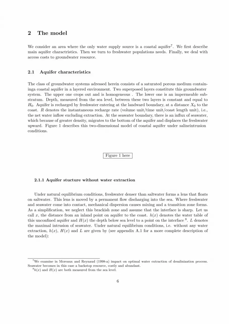
ing a coastal aquifer in a layered environment. Two superposed layers constitute this groundwatersystem. The upper one crops out and is homogeneous . The lower one is an impermeable sub-stratum. Depth, measured from the sea level, between these two layers is constant and equal toH0. Aquifer is recharged by freshwater entering at the landward boundary, at a distance X0 to thecoast. R denotes the instantaneous recharge rate (volume unit/time unit/coast length unit), i.e.,
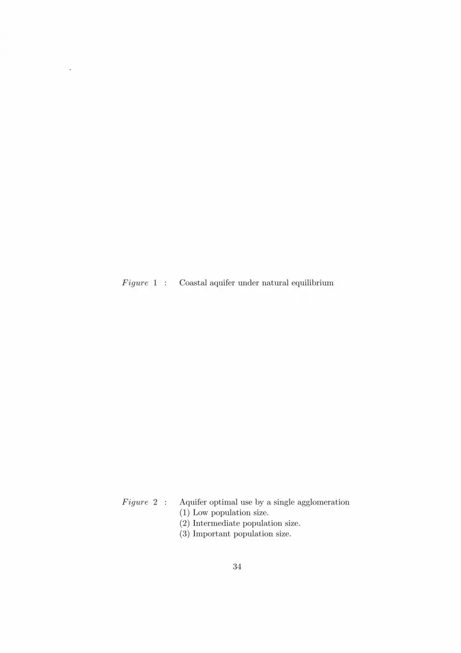
the net water inflow excluding extraction. At the seawater boundary, there is an influx of seawater,which because of greater density, migrates to the bottom of the aquifer and displaces the freshwaterupward. Figure 1 describes this two-dimensional model of coastal aquifer under saline intrusionconditions.
Figure 1 here
2.1.1 Aquifer stucture without water extraction
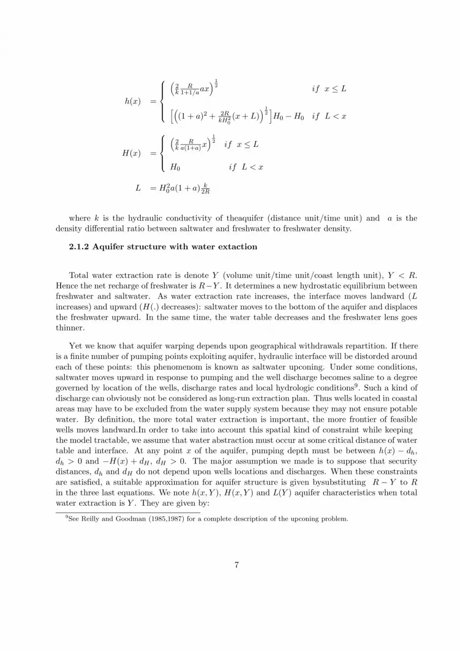
Under natural equilibrium conditions, freshwater denser than saltwater forms a lens that floatson saltwater. This lens is moved by a permanent flow discharging into the sea. Where freshwaterand seawater come into contact, mechanical dispersion causes mixing and a transition zone forms.
As a simplification, we neglect this brackish zone and assume that the interface is sharp. Let uscall x, the distance from an inland point on aquifer to the coast. h(x) denotes the water table ofthis unconfined aquifer and H(x) the depth below sea level to a point on the interface 8. L denotesthe maximal intrusion of seawater. Under natural equilibrium conditions, i.e. without any waterextraction, h(x), H(x) and L are given by (see appendix A.1 for a more complete description of
the model):
7We examine in Moreaux and Reynaud (1998-a) impact on optimal water extraction of desalinization process.Seawater becomes in this case a backstop resource, costly and abundant.
8h(x) and H(x) are both measured from the sea level.
6
h(x) =
(2k
R1+1/aax
) 12 if x ≤ L
[((1 + a)2 + 2R
kH20(x + L)
)12]H0 −H0 if L < x
H(x) =
(2k
Ra(1+a)x
)12
if x ≤ L
H0 if L < x
L = H20a(1 + a) k
2R
where k is the hydraulic conductivity of the aquifer (distance unit/time unit) and a is thedensity differential ratio between saltwater and freshwater to freshwater density.
2.1.2 Aquifer structure with water extaction
Total water extraction rate is denote Y (volume unit/time unit/coast length unit), Y < R.Hence the net recharge of freshwater is R−Y . It determines a new hydrostatic equilibrium betweenfreshwater and saltwater. As water extraction rate increases, the interface moves landward (L
increases) and upward (H(.) decreases): saltwater moves to the bottom of the aquifer and displacesthe freshwater upward. In the same time, the water table decreases and the freshwater lens goesthinner.
Yet we know that aquifer warping depends upon geographical withdrawals repartition. If thereis a finite number of pumping points exploiting aquifer, hydraulic interface will be distorded around
each of these points: this phenomenom is known as saltwater upconing. Under some conditions,saltwater moves upward in response to pumping and the well discharge becomes saline to a degreegoverned by location of the wells, discharge rates and local hydrologic conditions9. Such a kind ofdischarge can obviously not be considered as long-run extraction plan. Thus wells located in coastalareas may have to be excluded from the water supply system because they may not ensure potable
water. By definition, the more total water extraction is important, the more frontier of feasiblewells moves landward. In order to take into account this spatial kind of constraint while keepingthe model tractable, we assume that water abstraction must occur at some critical distance of watertable and interface. At any point x of the aquifer, pumping depth must be between h(x) − dh,dh > 0 and −H(x) + dH , dH > 0. The major assumption we made is to suppose that securitydistances, dh and dH do not depend upon wells locations and discharges. When these constraints
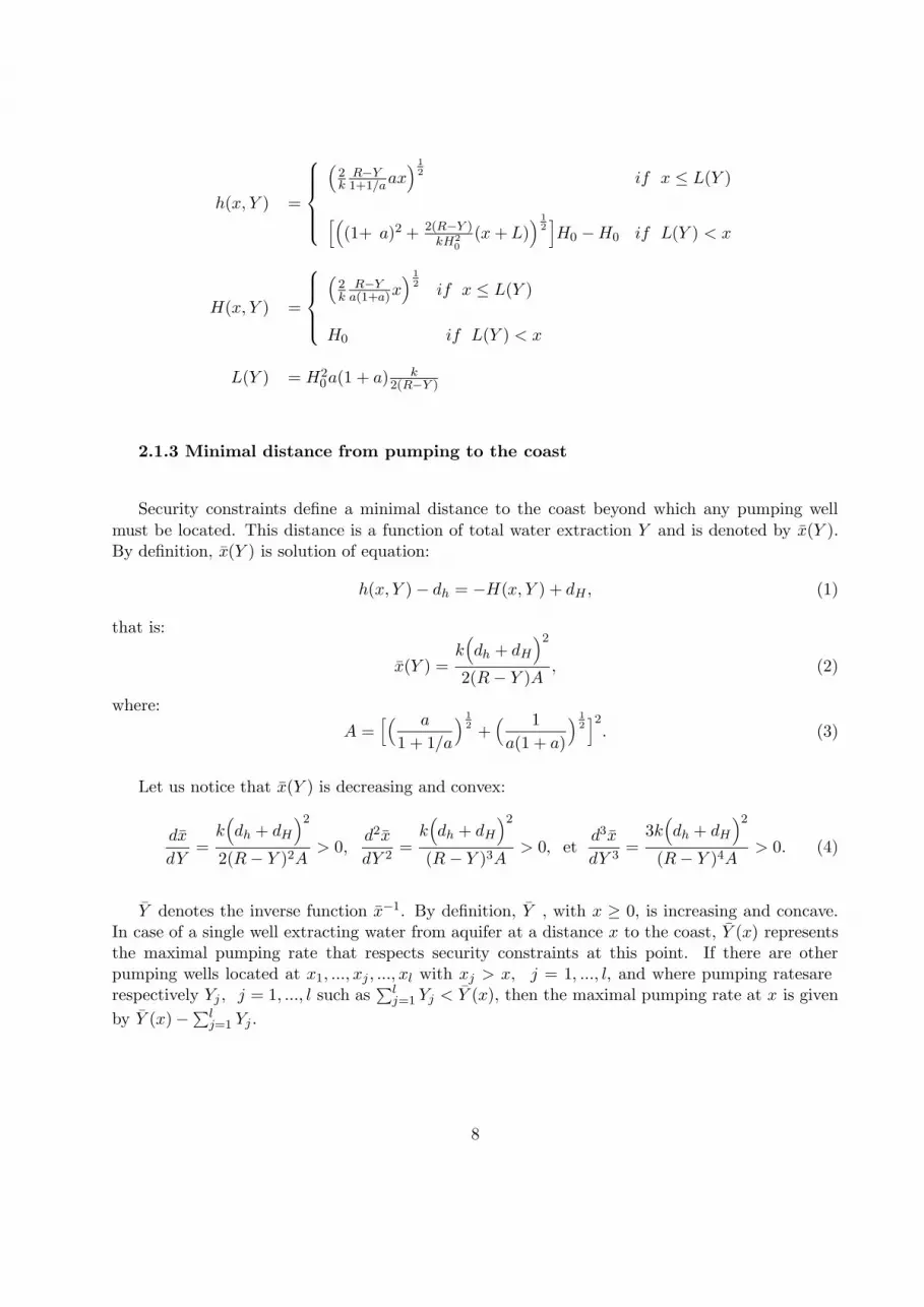
are satisfied, a suitable approximation for aquifer structure is given by substituting R − Y to Rin the three last equations. We note h(x, Y ), H(x, Y ) and L(Y ) aquifer characteristics when totalwater extraction is Y . They are given by:
9See Reilly and Goodman (1985,1987) for a complete description of the upconing problem.
7
h(x, Y ) =
(2k
R−Y1+1/aax
)12 if x ≤ L(Y )
[((1 + a)2 + 2(R−Y )
kH20
(x + L)) 1
2]H0 −H0 if L(Y ) < x
H(x, Y ) =
(2k
R−Ya(1+a)x
) 12
if x ≤ L(Y )
H0 if L(Y ) < x
L(Y ) = H20a(1 + a) k
2(R−Y )
2.1.3 Minimal distance from pumping to the coast
Security constraints define a minimal distance to the coast beyond which any pumping well
must be located. This distance is a function of total water extraction Y and is denoted by x(Y ).By definition, x(Y ) is solution of equation:
h(x, Y )− dh = −H(x, Y ) + dH , (1)
that is:
x(Y ) =k(dh + dH
)2
2(R− Y )A, (2)
where:
A =[( a
1 + 1/a
) 12
+( 1
a(1 + a)
) 12]2
. (3)
Let us notice that x(Y ) is decreasing and convex:
dx
dY=
k(dh + dH
)2
2(R− Y )2A> 0,
d2x
dY 2=
k(dh + dH
)2
(R − Y )3A> 0, et
d3x
dY 3=
3k(dh + dH
)2
(R− Y )4A> 0. (4)
Y denotes the inverse function x−1. By definition, Y , with x ≥ 0, is increasing and concave.In case of a single well extracting water from aquifer at a distance x to the coast, Y (x) representsthe maximal pumping rate that respects security constraints at this point. If there are otherpumping wells located at x1, ..., xj , ..., xl with xj > x, j = 1, ..., l, and where pumping rates arerespectively Yj , j = 1, ..., l such as
∑lj=1 Yj < Y (x), then the maximal pumping rate at x is given
by Y (x)−∑l
j=1 Yj .
8

2.2 Resource valorisation and costs
The coastal aquifer is exploited by I agglomerations indexed by i, i = 1, ..., I. x0i denotes the dis-
tance from agglomeration i to the coast. As a convention, agglomerations are indexed by increasing
distance to the coast: x01 < ... < x0
i < ... < x0I . We suppose that all agglomerations are composed
by identical individuals 10. ni denotes population size of agglomeration i. Thus consumption percapita is the same for all users living in the same agglomeration. We note yi, the instantaneouswater consumption per capita of agglomeration i, Yi = niyi, the total consumption of agglomera-tion i and Y =
∑i Yi the total water extraction of all agglomerations exploiting the coastal aquifer.
As a simplification, we will not distinguish between net and gross withdrawals: we assume thatall water abstraction if definitively lost for the groundwater system. The interested reader willfind in Moreaux and Reynaud (1998-b) a more complete study taking into account partial returnflows after use, networks leak and purification losses. Nevertheless, all these phenomenoms do notmodify qualitatively the results presented here.
The individual utility function depends solely on water consumption and is assumed to be the
same for all representative consumers. Utility fonction is denoted by U(.)11. We make the followingassumptions: utility function U is supposed as many times as necessary continuously differentiable,stricly increasing and concave and water is considered as an assential good:
dU
dy> 0,
d2U
dy2< 0, et lim
y→0
dU
dy= +∞. (5)
Because water consumption is identical for all individuals living in the same agglomeration, we candefine an aggregate utility function for any agglomeration. Vi denotes the aggregate utility functionof agglomeration i:
Vi(Yi) = niU(Yi/ni) (6)
Vi is stricly increasing and concave:
dVi
dYi=
dU
dyi
∣∣∣yi=Yi/ni
> 0,d2Vi
dY 2i
=1
ni
d2U
dy2i
∣∣∣yi=Yi/ni
< 0, et limYi→0
dVi
dYi= +∞. (7)
Total water supplying costs are constituted by pumping costs, surface conveyance costs anddistribution costs. Pumping costs depend both upon discharge of water and depth of pumping.
g(x) denotes the ground surface measured from the sea level so required water elevation at x isgiven by g(x)−h(x) where h(x) is the water table. For a stake of simplicity, we neglect this part ofpumping costs and assume that they just depend upon water discharge. We denote γ, γ > 0, theunit cost of pumping per unit of discharge. Total cost of pumping is: γY . Surface water conveyancefrom pumping point to agglomeration i is supposed proportional to the distance and the discharge.
We note β, β > 0 the unit conveyance cost per unit of distance and discharge. Thus the conveyancecost of agglomeration i pumping Yi from a well located in xi is: β | xi−x0
i | Yi. Finally, we assumethat distribution costs are proportional to water discharge. We note µ, µ > 0, the unit distribution
10Agglomerations are composed of identical representative individuals having the same activities, the same tastesand the same incomes.
11Utility is measured in monetary units.
9
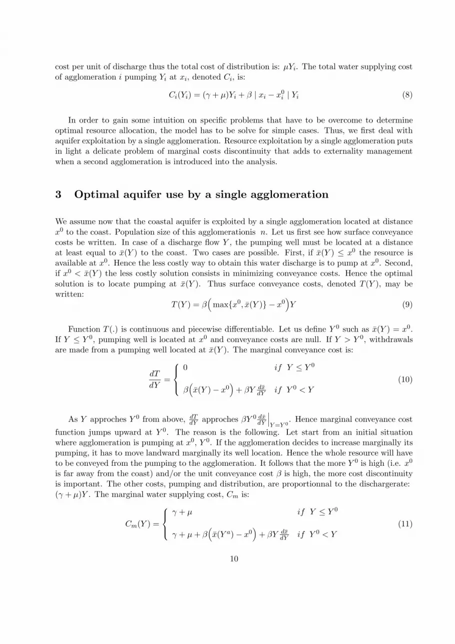
cost per unit of discharge thus the total cost of distribution is: µYi. The total water supplying costof agglomeration i pumping Yi at xi, denoted Ci, is:
Ci(Yi) = (γ + µ)Yi + β | xi − x0i | Yi (8)
In order to gain some intuition on specific problems that have to be overcome to determineoptimal resource allocation, the model has to be solve for simple cases. Thus, we first deal withaquifer exploitation by a single agglomeration. Resource exploitation by a single agglomeration putsin light a delicate problem of marginal costs discontinuity that adds to externality management
when a second agglomeration is introduced into the analysis.
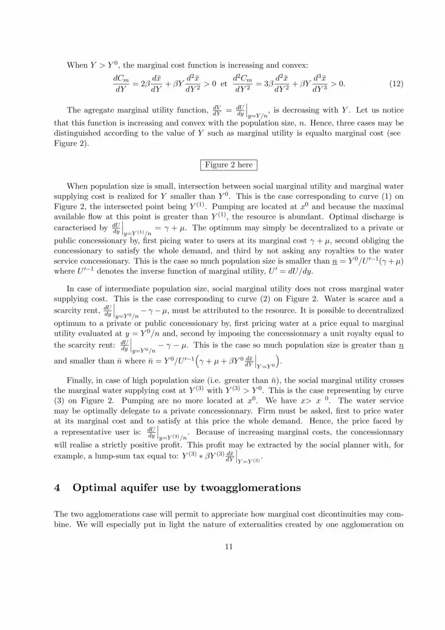
3 Optimal aquifer use by a single agglomeration
We assume now that the coastal aquifer is exploited by a single agglomeration located at distance
x0 to the coast. Population size of this agglomeration is n. Let us first see how surface conveyancecosts be written. In case of a discharge flow Y , the pumping well must be located at a distanceat least equal to x(Y ) to the coast. Two cases are possible. First, if x(Y ) ≤ x0 the resource isavailable at x0. Hence the less costly way to obtain this water discharge is to pump at x0. Second,if x0 < x(Y ) the less costly solution consists in minimizing conveyance costs. Hence the optimal
solution is to locate pumping at x(Y ). Thus surface conveyance costs, denoted T (Y ), may bewritten:
T (Y ) = β(
max{x0, x(Y )} − x0)Y (9)
Function T (.) is continuous and piecewise differentiable. Let us define Y 0 such as x(Y ) = x0.If Y ≤ Y 0, pumping well is located at x0 and conveyance costs are null. If Y > Y 0, withdrawalsare made from a pumping well located at x(Y ). The marginal conveyance cost is:
dT
dY=
0 if Y ≤ Y 0
β(x(Y )− x0
)+ βY dx
dY if Y 0 < Y(10)
As Y approches Y 0 from above, dTdY approches βY 0 dx
dY
∣∣∣Y =Y 0
. Hence marginal conveyance cost
function jumps upward at Y 0. The reason is the following. Let start from an initial situationwhere agglomeration is pumping at x0, Y 0. If the agglomeration decides to increase marginally itspumping, it has to move landward marginally its well location. Hence the whole resource will haveto be conveyed from the pumping to the agglomeration. It follows that the more Y 0 is high (i.e. x0
is far away from the coast) and/or the unit conveyance cost β is high, the more cost discontinuityis important. The other costs, pumping and distribution, are proportionnal to the discharge rate:
(γ + µ)Y . The marginal water supplying cost, Cm is:
Cm(Y ) =
γ + µ if Y ≤ Y 0
γ + µ + β(x(Y a)− x0
)+ βY dx
dY if Y 0 < Y
(11)
10
When Y > Y 0, the marginal cost function is increasing and convex:
dCm
dY= 2β
dx
dY+ βY
d2x
dY 2> 0 et
d2Cm
dY 2= 3β
d2x
dY 2+ βY
d3x
dY 3> 0. (12)
The agregate marginal utility function, dVdY = dU
dy
∣∣∣y=Y/n
, is decreasing with Y . Let us notice
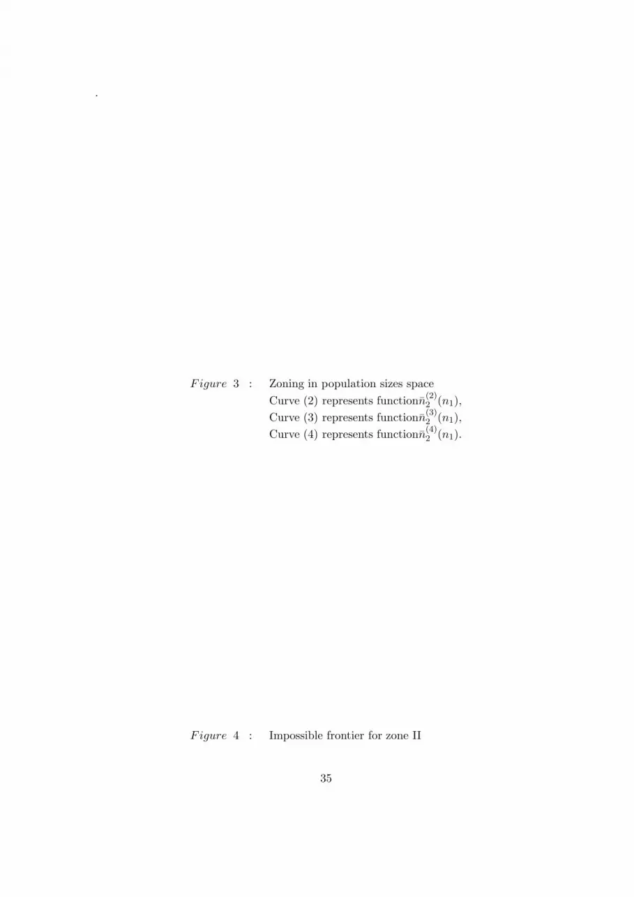
that this function is increasing and convex with the population size, n. Hence, three cases may bedistinguished according to the value of Y such as marginal utility is equal to marginal cost (see
Figure 2).
Figure 2 here
When population size is small, intersection between social marginal utility and marginal watersupplying cost is realized for Y smaller than Y 0. This is the case corresponding to curve (1) on
Figure 2, the intersected point being Y (1). Pumping are located at x0 and because the maximalavailable flow at this point is greater than Y (1), the resource is abundant. Optimal discharge is
caracterised by dUdy
∣∣∣y=Y (1)/n
= γ + µ. The optimum may simply be decentralized to a private or
public concessionary by, first picing water to users at its marginal cost γ + µ, second obliging theconcessionary to satisfy the whole demand, and third by not asking any royalties to the water
service concessionary. This is the case so much population size is smaller than n = Y 0/U ′−1(γ +µ)where U ′−1 denotes the inverse function of marginal utility, U ′ = dU/dy.
In case of intermediate population size, social marginal utility does not cross marginal watersupplying cost. This is the case corresponding to curve (2) on Figure 2. Water is scarce and a
scarcity rent, dUdy
∣∣∣y=Y 0/n
− γ −µ, must be attributed to the resource. It is possible to decentralized
optimum to a private or public concessionary by, first pricing water at a price equal to marginalutility evaluated at y = Y 0/n and, second by imposing the concessionnary a unit royalty equal to
the scarcity rent: dUdy
∣∣∣y=Y 0/n
− γ − µ. This is the case so much population size is greater than n
and smaller than n where n = Y 0/U ′−1(γ + µ + βY 0 dx
dY
∣∣∣Y =Y 0
).
Finally, in case of high population size (i.e. greater than n), the social marginal utility crossesthe marginal water supplying cost at Y (3) with Y (3) > Y 0. This is the case representing by curve(3) on Figure 2. Pumping are no more located at x0. We have x > x0. The water service
may be optimally delegate to a private concessionnary. Firm must be asked, first to price waterat its marginal cost and to satisfy at this price the whole demand. Hence, the price faced by
a representative user is: dUdy
∣∣∣y=Y (3)/n
. Because of increasing marginal costs, the concessionnary
will realise a strictly positive profit. This profit may be extracted by the social planner with, for
example, a lump-sum tax equal to: Y (3) ∗ βY (3) dxdY
∣∣∣Y =Y (3)
.
4 Optimal aquifer use by two agglomerations
The two agglomerations case will permit to appreciate how marginal cost dicontinuities may com-
bine. We will especially put in light the nature of externalities created by one agglomeration on
11
the other one. We suppose now that aquifer is exploited by two agglomerations indexed by 1 and2 and located at x0
1 and x02, x0
1 < x02. Population sizes are respectively n1 and n2. As a convention,
agglomeration 1 is called downstream whereas upstream denotes agglomeration 2. In the same
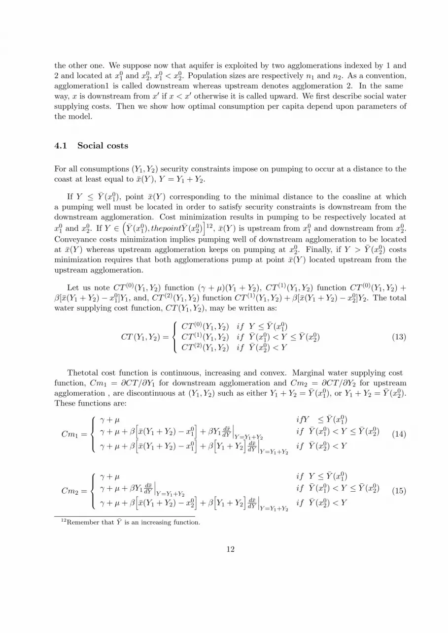
way, x is downstream from x′ if x < x′ otherwise it is called upward. We first describe social watersupplying costs. Then we show how optimal consumption per capita depend upon parameters ofthe model.
4.1 Social costs
For all consumptions (Y1, Y2) security constraints impose on pumping to occur at a distance to thecoast at least equal to x(Y ), Y = Y1 + Y2.
If Y ≤ Y (x01), point x(Y ) corresponding to the minimal distance to the coasline at which
a pumping well must be located in order to satisfy security constraints is downstream from thedownstream agglomeration. Cost minimization results in pumping to be respectively located at
x01 and x0
2. If Y ∈(Y (x0
1), thepointY (x02)
]12, x(Y ) is upstream from x0
1 and downstream from x02.
Conveyance costs minimization implies pumping well of downstream agglomeration to be locatedat x(Y ) whereas upstream agglomeration keeps on pumping at x0
2. Finally, if Y > Y (x02) costs
minimization requires that both agglomerations pump at point x(Y ) located upstream from the
upstream agglomeration.
Let us note CT (0)(Y1, Y2) function (γ + µ)(Y1 + Y2), CT (1)(Y1, Y2) function CT (0)(Y1, Y2) +β[x(Y1 + Y2)− x0
1]Y1, and, CT (2)(Y1, Y2) function CT (1)(Y1, Y2) + β[x(Y1 + Y2)− x02]Y2. The total
water supplying cost function, CT (Y1, Y2), may be written as:
CT (Y1, Y2) =
CT (0)(Y1, Y2) if Y ≤ Y (x01)
CT (1)(Y1, Y2) if Y (x01) < Y ≤ Y (x0
2)
CT (2)(Y1, Y2) if Y (x02) < Y
(13)
The total cost function is continuous, increasing and convex. Marginal water supplying costfunction, Cm1 = ∂CT/∂Y1 for downstream agglomeration and Cm2 = ∂CT/∂Y2 for upstreamagglomeration , are discontinuous at (Y1, Y2) such as either Y1 + Y2 = Y (x0
1), or Y1 + Y2 = Y (x02).
These functions are:
Cm1 =
γ + µ if Y ≤ Y (x01)
γ + µ + β[x(Y1 + Y2)− x0
1
]+ βY1
dxdY
∣∣∣Y =Y1+Y2
if Y (x01) < Y ≤ Y (x0
2)
γ + µ + β[x(Y1 + Y2)− x0
1
]+ β
[Y1 + Y2
]dxdY
∣∣∣Y =Y1+Y2
if Y (x02) < Y
(14)
Cm2 =
γ + µ if Y ≤ Y (x01)
γ + µ + βY1dxdY
∣∣∣Y =Y1+Y2
if Y (x01) < Y ≤ Y (x0
2)
γ + µ + β[x(Y1 + Y2)− x0
2
]+ β
[Y1 + Y2
]dxdY
∣∣∣Y =Y1+Y2
if Y (x02) < Y
(15)
12Remember that Y is an increasing function.
12
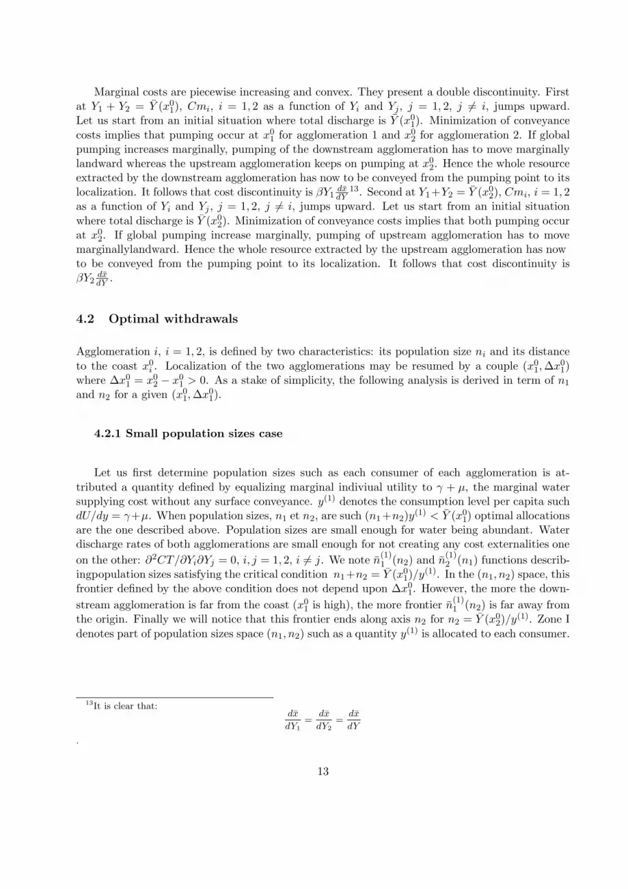
Marginal costs are piecewise increasing and convex. They present a double discontinuity. Firstat Y1 + Y2 = Y (x0
1), Cmi, i = 1, 2 as a function of Yi and Yj, j = 1, 2, j 6= i, jumps upward.Let us start from an initial situation where total discharge is Y (x0
1). Minimization of conveyance
costs implies that pumping occur at x01 for agglomeration 1 and x0
2 for agglomeration 2. If globalpumping increases marginally, pumping of the downstream agglomeration has to move marginallylandward whereas the upstream agglomeration keeps on pumping at x0
2. Hence the whole resourceextracted by the downstream agglomeration has now to be conveyed from the pumping point to itslocalization. It follows that cost discontinuity is βY1
dxdY
13. Second at Y1+Y2 = Y (x02), Cmi, i = 1, 2
as a function of Yi and Yj , j = 1, 2, j 6= i, jumps upward. Let us start from an initial situation
where total discharge is Y (x02). Minimization of conveyance costs implies that both pumping occur
at x02. If global pumping increase marginally, pumping of upstream agglomeration has to move
marginally landward. Hence the whole resource extracted by the upstream agglomeration has nowto be conveyed from the pumping point to its localization. It follows that cost discontinuity isβY2
dxdY .
4.2 Optimal withdrawals
Agglomeration i, i = 1, 2, is defined by two characteristics: its population size ni and its distance
to the coast x0i . Localization of the two agglomerations may be resumed by a couple (x0
1, ∆x01)
where ∆x01 = x0
2 − x01 > 0. As a stake of simplicity, the following analysis is derived in term of n1
and n2 for a given (x01, ∆x0
1).
4.2.1 Small population sizes case
Let us first determine population sizes such as each consumer of each agglomeration is at-
tributed a quantity defined by equalizing marginal indiviual utility to γ + µ, the marginal watersupplying cost without any surface conveyance. y(1) denotes the consumption level per capita suchdU/dy = γ+µ. When population sizes, n1 et n2, are such (n1+n2)y
(1) < Y (x01) optimal allocations
are the one described above. Population sizes are small enough for water being abundant. Waterdischarge rates of both agglomerations are small enough for not creating any cost externalities one
on the other: ∂2CT/∂Yi∂Yj = 0, i, j = 1, 2, i 6= j. We note n(1)1 (n2) and n
(1)2 (n1) functions describ-
ing population sizes satisfying the critical condition n1+n2 = Y (x01)/y(1). In the (n1, n2) space, this
frontier defined by the above condition does not depend upon ∆x01. However, the more the down-
stream agglomeration is far from the coast (x01 is high), the more frontier n
(1)1 (n2) is far away from
the origin. Finally we will notice that this frontier ends along axis n2 for n2 = Y (x02)/y(1). Zone I
denotes part of population sizes space (n1, n2) such as a quantity y(1) is allocated to each consumer.
13It is clear that:dx
dY1=
dx
dY2=
dx
dY
.
13

4.2.2 Relatively small population sizes case
Let us now consider population sizes ouside zone I. The first problem is to determine if it isefficient or not to increase global pumping. A total discharge rate increase will move the down-
stream agglomeration pumping point landward. Hence the downstream agglomeration has to bearconveyance costs. Intuition suggests in this case that it is not optimal to increase total with-drawals as much (n1, n2) is near from the geometrical locus n1 + n2 = Y (x0
1)/y(1). The optimalsolution would consist in restricting pumping at Y (x0
1) and, because total supplying costs do notdepend upon population repartition between the two agglomerations, in equalizing marginal util-
ities between consumers. Hence, the same discharge rate Y (x01)/(n1 + n2) has to be attributed
to all users14. y(2) denotes this water consumption per capita. A scarcity rent λ(2), equal todUdy
∣∣∣y=y(2)(n1,n2)
− (γ + µ) > 0, is associated to the resource. This solution prevails as much the
scarcity rent is smaller than marginal social coast discontinuity, i.e. while:
dU
dy
∣∣∣y=y(2)
− (γ + µ) ≤ βn1
n1 + n2Y (x0
1)dx
dY
∣∣∣Y =Y (x0
1)(16)
We will notice that for n1 fixed, the left handside term of this inequality is an increasingfunction of n2 going to infinity as n2 goes to infinity The right handside term is a decreasingfunction of n2 going to 0 as n2 goes to infinity. Hence given n1, there exists a single n2 denoted
n(2)2 (n1) < +∞, n
(2)2 (n1) > n
(1)2 (n1), verifying inequality (16) as an equality. Function n
(2)2 (n1) is
defined for n1 smaller than solution of dUdy
∣∣∣y=Y (x0
1)/n1
− (γ + µ) = βY (x01)
dxdY
∣∣∣Y =Y (x0
1)denoted by
n(2)1 , n
(2)1 > Y (x0
1)/y(1)15. We have n(2)2 (n
(2)1 ) = 0 and limn1→0 n
(2)2 (n1) = Y (x0
1)/y(1).
Given n2, the left handside term of inequality (16) is an increasing function of n1 going toinfinity as n1 goes to infinity. The right handside is an increasing function going to the finite value
βY (x01)
dxdY
∣∣∣Y =Y (x0
1)as n1 goes to infinity. Given n2, it is not possible to exclude that there exists
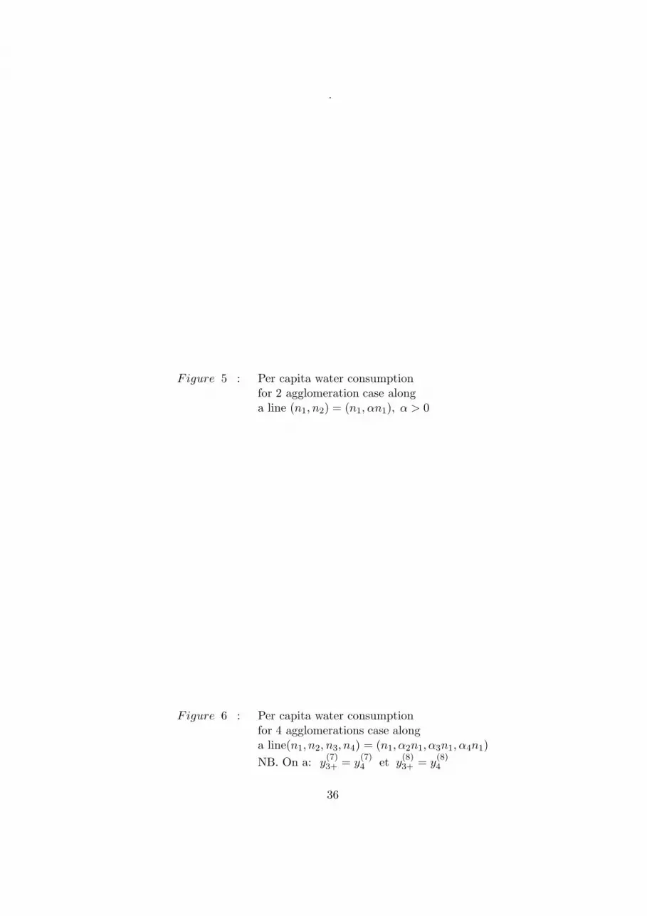
different n1, such as inequality (16) is verified as an equality. The North-East frontier of such azone would typically be the one described on Figure 316. On the other hand, the one discribed byFigure 4 is excluded.
Figure 3 ici
Figure 4 ici
Zone II denotes part of population sizes space (n1, n2) such optimal consumptions are the onewe have depicted above. In this zone, each user is attributed a quantity Y (x0
1)/(n1 + n2) andagglomeration 1 and 2 pumping occur respectively at x0
1 and x02. It is possible to delegate water
service to a private or public firm by making upstream agglomeration consumers internalize cost
14This result holds because all individuals have the same utility function.15Population size n
(2)1 corresponds to n defined in the one agglomeration case.
16See appendix A.2 for an other demonstration of this result.
14
externalities created by their withdrawals on downstream agglomeration consumers. Such wouldbe the case by imposing on firms a unit tax λ(2). If firms are asked, first to price water at theirmarginal cost including the unit royalty and, second to satisfy the whole demand at this price then
water discharges and pumping localizations will be optimal. This is the only case where, resourcebeing scarce, it is possible to decentralized water management with a single tax. Let us finallynotice that price faced by consumers is the same in both agglomeration, social marginal cost in-cluding tax being identical.
4.2.3 Relatively important population sizes case
Suppose now that population sizes are relatively important, that is (n1, n2) does not belong to
zone I and II but is not too far from the North-East frontier of zone II defined by curve n(2)2 (n1).
In such a case, the downstream agglomeration exploits the coastal aquifer from a point locatedupstream from x0
1 but downstream from x02. The upstream agglomeration keeps on exploiting
aquifer from x02. Marginal social costs are now different in both agglomerations. For the downstream
agglomeration, marginal social cost is equal to marginal “private” cost, i.e.:
Cm1(Y1, Y2) = γ + µ + β[x(Y1 + Y2)− x0
1
]+ βY1
dx
dY
∣∣∣Y =Y1+Y2
.
For the upstream agglomeration, marginal social cost is greater than marginal “private” cost, γ+µ:
Cm2(Y1, Y2) = γ + µ + βY1dx
dY
∣∣∣Y =Y1+Y2
> γ + µ.
Difference between marginal social cost and private social cost is due to cost externality created byupstream agglomeration on downstream one: by increasing its withdrawals, the upstream agglomer-
ation obliges the downstream agglomeration to move its pumping landward. Thus the downstreamagglomeration has to support greater conveyance costs.
Let us note y(3)1 and y
(3)2 optimal consumption per capita in agglomeration 1 and 2. These
consumptions are defined such as marginal utility is equal to the marginal social cost. Hence, the
couple (y(3)1 , y
(3)2 ) is solution of the following system in (y1, y2):
dU
dy
∣∣∣y=y1
= γ + µ + β[x(n1y1 + n2y2)− x0
1
]+ βn1y1
dx
dY
∣∣∣Y =n1y1+n2y2
(17)
dU
dy
∣∣∣y=y2
= γ + µ + βn1y1dx
dY
∣∣∣Y =n1y1+n2y2
(18)
Assumption of decreasing marginal utility implies that y(3)1 < y
(3)2 whatever are population sizes of
the two agglomerations.
Zone III denotes part of population sizes space (n1, n2) such as optimal consumption are theone we just have described above. What is the North-East frontier of this area? This frontier istouched when the downstream agglomeration has to exploit aquifer at x0
2. Hence this frontier isdefined by:
x(n1y
(3)1 + n2y
(3)2
)≤ x0
2, (19)
15
where y(3)1 et y
(3)2 solutions of (17)-(18) depend upon n1 et n2. We show in Appendix A.3 that
given n1, there exists a single n2, denoted n(3)2 (n1), such as equations (17)-(18) are satisfied and
the weak inequality (19) is verified as an equality. Therefore as in the case of zone II North-Eastfrontier, it is not possible to exlude that given n2, there exists different n1 verifying (17)-(18) and
inequality (19) as an equality. Typically, the shape of n(3)2 (n1) is the one described on Figure 3.
Let us finally notice some characteristics of curve n(3)2 (n1). First, when n1 approches 0 from above,
n(3)2 (n1) approches Y (x0
2)/y(1) from below. This is a consequence of the fact that if n1 approaches
O from above, because y(3)1 is bounded by y(1), social marginal cost of upstream agglomeration,
γ + µ + βn1y(3)1
dxdY , approches γ + µ from above. Remember that if marginal cost is γ + µ, then
consumption per capita is y(1). It follows that limn1→0 n(3)2 (n1) = Y (x0
2)/y(1). Second, for anycouple (n1, n2) such as n1 > 0, n2 > 0 and n1 + n2 = Y (x0
2)/y(1), the marginal water supplying
cost of both agglomerations is greater than γ + µ. In that case y(3)1 < y(1) and y
(3)2 < y(1). As a
consequence, n(3)2 (n1) > [Y (x0
2)/y(1)]− n1. The frontier n(3)2 (n1) is located above the straight line
defined by n1 + n2 = Y (x02)/y(1) for n1 > 0. Last, n
(3)2 (n1) is equal to zero for n1 greater than
Y (x02)/y(1). This is a consequence of the fact that if n2 = 0, the marginal cost of water supplying
of downstream agglomeration is γ +µ+β(x02−x1
2)+βY (x02)
dxdY
∣∣∣Y =Y (x0
2), strictly greater than γ +µ.
So, we have y(3)1 < y(1). n
(3)1 denotes the value of n1 such as n
(3)2 (n1) = 0.
How it is possible to decentralize aquifer management in zone III? The social marginal cost ofdownstream agglomeration is equal to its private cost. It is possible to delegate water service to aprivate or public firm by first, pricing water at its marginal social cost and second, obliging the con-cessionnaries to satisfy the whole demand. Because of increasing marginal costs, the firm will realizepositive profits that may be extracted by a lump-sum tax. The social marginal cost of downstream
agglomeration is greater than its private cost. The concessionnary of water service in the upstream
agglomeration will act optimally only if it has to pay a unit royalty λ(3) = βn1y(3)1
dxdY
∣∣∣Y =n1y
(3)1 +n2y
(3)2
.
This unit fee make consumers of upstream agglomeration internalized externalities created by theirwithdrawals. Let us finally notice that consumers of agglomeration 1 and 2 will face different pricesbecause marginal social costs are different over aquifer.
4.2.4 Important population sizes case
Let us now consider population sizes (n1, n2) outside zone I, II and III. If (n1, n2) is not too far
from frontier n(3)2 (n1) , the problem is now to determine if it is efficient or not to maintain total
water discharge at a level Y (x02), or if it is socially better to increase pumping. In such a case the
social marginal cost jumps upward.
If total withdrawals are limited at Y (x02) pumping occur at x0
2. Water allocation among thetwo agglomerations must be realized according to the following principle. A marginal transfertdY1 from downstream agglomeration users to upstream agglomeration users has the two following
welfare effects:
16
– reduction of net social welfare in downstream agglomeration that may be approximatedat first order by: {dU
dy
∣∣∣y=Y1/n1
− (γ + µ)− β[x02 − x0
1]}dY1,
– increase of net social welfare in upstream agglomeration that may be approximated atfirst order by: {dU
dy
∣∣∣y=Y2/n2
− (γ + µ)}dY1.
In case of an optimal allocation this transfert dY1 doesn’t increase net global social welfare. Sumof the two terms above must be null. From this tradeoff condition and using the fact that total
water consumption is Y (x02), optimal consumption per capita in the two agglomeration, denoted
y(4)1 and y
(4)2 solves the following system in y1 et y2:
dU
dy
∣∣∣y=y1
− β[x02 − x0
1] =dU
dy
∣∣∣y=y2
(20)
n1y1 + n2y2 = Y (x02). (21)
Because dU/dy is decreasing with y, optimal water consumption in downstream agglomeration, y(4)1
is smaller than consumption in upstream agglomeration, y(4)2 . Zone IV denotes part in population
space (n1, n2) for which total withdrawals are Y (x02) and consumptions per capita are those deter-
mined by (20) and (21). What is the North-East frontier of this zone? If an agglomeration wantsto increase its consumption, the social marginal cost will be:
– for downstream agglomeration:
(γ + µ) + β[x02 − x0
1] + βY (x02)
dx
dY
∣∣∣Y =Y (x0
2),
– for upstream agglomeration:
(γ + µ) + βY (x02)
dx
dY
∣∣∣Y =Y (x0
2),
Hence zone IV is defined by the condition:
dU
dy
∣∣∣y=y
(4)1
− (γ + µ)− β[x02 − x0
1] =dU
dy
∣∣∣y=y
(2)2
− (γ + µ) = βY (x02)
dx
dY
∣∣∣Y =Y (x0
2), (22)
where the first equality is a direct consequence of (20). As in the case of zone II and III, it
can be shown that given n1, there exists a single n2, denoted n(4)2 (n1), such as equations (20),
(21) and (19) are satified. We show in Appendix A.4 that function n(4)2 (n1) is not necessary
monotonous. Moreover, limn1→0 n(4)2 (n1) > Y (x0
2)/y(1). In fact, limn1→0 n(4)2 (n1) is equal to n
defined in the one agglomeration case. Otherwise, function n(4)2 (n1) is null for n1 = n
(3)1 . If
there is only one agglomeration located in x01, when Y1 = Y (x0
2), its marginal private cost is
γ + µ + β[x02 − x0
1] + βY (x02)
dxdY
∣∣∣Y =Y (x0
2).
17
When population sizes belong to zone IV, decentralization of the optimum may be organ-ised as follows. The social marginal cost of downstream agglomeration, (γ + µ) + β[x0
2 − x01] +
βY (x02)
dxdY
∣∣∣Y =Y (x0
2)is greater than its marginal “private” cost, (γ+µ)+β[x0
2−x01]+βn1y
(4)1
dxdY
∣∣∣Y =Y (x0
2).
Delegate firm of the downstream agglomeration must price water at its marginal cost including a
unit royalty λ(4)1 = n2y
(4)2
dxdY
∣∣∣Y =Y (x0
2), and must satisfy the whole demand. Upstream agglomeration
concessionary has to pay a unit royalty λ(4)2 = βY (x0
2)dxdY
∣∣∣Y =Y (x0
2), λ
(4)2 > λ
(4)1 corresponding to the
difference between its marginal social cost and its marginal private cost. Optimum decentralizationrequires a differenciate system of taxes.
4.2.5 Very important population sizes case
Finally we examine the case of very important population sizes that is populations that do notbelong to zone I to IV. Because pumping are now located at x(Y1 +Y2) > x0
2, marginal social costsare respectively:
– for the downstream agglomeration:
(γ + µ) + β[x(Y1 + Y2)− x01] + β[Y1 + Y2]
dx
dY
∣∣∣Y =Y1+Y2
,
– for the upstream agglomeration:
(γ + µ) + β[x(Y1 + Y2)− x02] + β[Y1 + Y2]
dx
dY
∣∣∣Y =Y1+Y2
.
Optimal consumption per capita in agglomerations 1 and 2, y(5)1 and y
(5)2 , are solution of the
following system in y1 et y2:
dU
dy
∣∣∣y=y1
= (γ + µ) + β[x(n1y1 + n2y2)− x01] + β[n1y1 + n2y2]
dx
dY
∣∣∣Y =n1y1+n2y2
, (23)
dU
dy
∣∣∣y=y2
= (γ + µ) + β[x(n1y1 + n2y2)− x02] + β[n1y1 + n2y2]
dx
dY
∣∣∣Y =n1y1+n2y2
. (24)
Consumption per capita in the downstream agglomeration, y(5)1 , is still smaller than consumption in
the upstream agglomeration y(5)2 where the marginal social cost is smaller, whatever are populations
in this area that will be denoted zone V.
Water must be sold at price dUdy
∣∣∣y=y
(5)1
in downstream agglomeration and at price dUdy
∣∣∣y=y
(5)2
in the upstream one. Hence, price in the downstream agglomeration is greater than price inthe upward agglomeration. The private marginal water supplying cost of agglomeration i is
γ + µ + β[x(niy(5)i + njy
(5)j ) − x0
i ] + β[niy(5)i ] dx
dY
∣∣∣Y =niy
(5)i +njy
(5)j
, i 6= j. Hence, difference between
social and private marginal cost for agglomeration i is βnjy(5)j
dxdY
∣∣∣Y =niy
(5)i +njy
(5)j
. The difference
depends upon population sizes of agglomerations. By imposing upon each concessionnary a royalty
18
corresponding to this difference and by asking him to maximize its profits, he will offer optimalquantities pumped at a optimal localization. Moreover, and it will be admitted with difficulty byusers17, the more population of one agglomeration is small in proportion to the total population,
the more the unit royalty will be high because its cost externality is the highest. Water servicedecentralisation still requires a differenciate tax system. Let us finally notice that private marginal
costs are greater than average costs, difference for agglomeration i being βniy(5)i
dxdY
∣∣∣Y =niy
(5)i +njy
(5)j
.
Concessionnaries of both agglomerations will realize positive prifits that may be extracted by thesocial planner with a lump-sum tax.
4.2.6 Per capita consumptions and population sizes
Figure 4 gives per capita optimal consumption depending upon population sizes of the two ag-glomeration, the ratio of population sizes keeping on constant along a line (n1, n2) = (n1, αn1), α >0. This consumption are identical while global population is not too important, consumption percapita in downstream agglomeration being smaller than in upstream agglomeration farther.
Figure 4 here
17Experience shows that margin analysis are in general not understood and that their consequences are acceptedwith difficulty.
19
5 Generalization to any number of agglomeration
The optimal water allocation method, as described in details for the two agglomerations case, canquite easily be generalized to any number, I , of agglomerations. Let’s keep the same presentation
as in previous section.
If population size is low, the resource is abundant and each agglomeration may pump whereit is located. Social and marginal costs are equal to γ + µ in this case. As population size raises,security constraints respect requires some of the agglomerations (the ones located near the coast)pump upstream from where they are located, while the other pump where they are located. In theone agglomeration case, there were three population sizes classes each one defining three different
optimal consumption systems. In the two agglomerations case, there were five population sizesvectors classes each one defining five different optimal consumption systems. It follows that in theI agglomerations case, 2I + 1 population size vectors classes will define 2I + 1 different optimalconsumption systems.
Let’s examine how optimal water uses are determined in the case of population sizes classes1, 2, ..., 2i, 2i + 1 et 2I + 1. In this section we assume that the Is population sizes are strictly
positive.
5.1 Population sizes class of rank 1
When the population sizes are very low, each agglomeration can exploit aquifer where it is located.Therefore, this zone is the same as the one noted zone I in the two agglomerations case.
Because agglomerations pump where they are located, each one faces a marginal social cost ofγ + µ. Per capita consumption is thus the same in each agglomeration. It is equal to y(1) definedby:
dU
dy= γ + µ.
This solution prevails while the condition∑
i ni < Y (x0i )/y(1) is satisfied. Water is abundant with
respect to population sizes and its management is not a real problem.
5.2 Population sizes class of rank 2
Total population size is higher than Y (x0i )/y(1), but not high enough to make the pumping minimal
distance to the coast be greater than x01. Each agglomeration pumps where is is located with
marginal cost equal to γ + µ. The total discharge rate is Y (x0i ), the aggregate water flow for
which safety the minimal distance is exactely x01. As access costs do not depend upon population
repartition among agglomeration, social welfare is maximized by allocating the same water dischargerate to each consumer. If N denotes the aggregate population size, we have N =
∑Ii=1 ni and per
capita consumption must be equal y(2) = Y (x01)/N in every agglomeration.
20
If agglomeration i wants to raise marginally its consumption by dYi beyon Y(2)i = niy
(2),
other agglomerations discharge rates still being Y(2)j = njy
(2), the marginal social cost increase
is[γ + µ + βY
(2)1
dxdY
∣∣∣Y =Y (x0
1)
]dYi as agglomeration 1 has to move landward upstream from x0
1 its
pumping point whereas other agglomerations keep on pumping where they are located. The limitcondition defining zone 2 frontier is thus:
dU
dy
∣∣∣y=Y (x0
1)/N− (γ + µ) = β
n1
NY (x0
1)dx
dY
∣∣∣Y =Y (x0
1). (25)
It follows that the maximal admissible population size depends upon n1. Let’s N(1) denote thewhole population size for agglomeration 2 to I. The frontier, studied in details in appendix 5, may
be described by a function N(2)(1) (n1) that determines maximal population size for agglomeration 2 to
I , as a function of n1. Given n1 small enough , if population sizes nh of agglomerations h = 2, ..., I
are such as∑
h 6=1 nh = N(2)(1) (n1) then (n1, ..., nI) belongs to zone 2 frontier. Function N
(2)(1) is not
necessary monotonous.
Inside zone 2, we have:
dU
dy> γ + µ.
Let λ(2) denote the difference dUdy −(γ+µ). λ(2) is the scarcity rent of resource. Its management can
be decentralized by single unit tax λ(2), for all agglomerations. Each water service concessionnaryhas to price water at its marginal cost including the unit fee and to satisfy the whole demand that
he faces.
5.3 Population sizes classes of rank 2i
In each population size of rank 2i, i = 1, ..., I , water discharge rate is Y (x0i ). Agglomerations
k = 1, ..., i − 1 withdraw from x0i > x0
k, and agglomerations k = i, ..., I pump where they arelocated. We remain in this population zone while population sizes aren’t high enough to moveupstream from x0
i pumping point of agglomeration 1, ..., i − 1. As total water discharge rate isY (x0
i ), optimality conditions may be expressed as follows. At optimum, social welfare may not be
improved:
– by transfering an amount dYk of consumption from agglomeration k < i− 1, to agglom-eration k′, k < k′ ≤ i− 1, so that for each agglomerations couple (k, k′):
dU
dy
∣∣∣y=yk
− β[x0i − x0
k] =dU
dy
∣∣∣y=yk′
− β[x0i − x0
k′ ],
– by transfering an amount dYk of consumption from agglomeration k < i−1, to k′, k′ ≥ i,so that so that for each agglomerations couple (k, k′):
dU
dy
∣∣∣y=yk
− β[x0i − x0
k] =dU
dy
∣∣∣y=yk′
,
21
– by transfering an amount dYk of consumption from agglomeration k ≥ i, to agglomera-tion k′, k′ ≥ i, k 6= k′, so that for each agglomerations couple (k, k′):
dU
dy
∣∣∣y=yk
=dU
dy
∣∣∣y=yk′
.
Per capita consumption must clearly by the same in each agglomeration k = i, ..., I. Let yi+ denoteper capita consumption in one of those agglomerations. In this zone, optimal consumption per
capita, y(2i)1 , ..., y
(2i)i−1 , y
(2i)i+ are the ones that solve the following equation system in y1, ..., yi, yi+:
dU
dy
∣∣∣y=yk
− β[x0i − x0
k] =dU
dy
∣∣∣y=yi+
, k = 1, ..., i− 1 (26)
i−1∑
k=1
nkyk + Ni+yi+ = Y (x0i ) (27)
where Ni+ is total population of agglomerations h = i, ..., I . Given assumptions about U , the moreagglomerations k = 1, ..., i are far away from the coast, the more optimal per capita consumption
y(2i)1 < ... < y
(2i)k < ... < y
(2i)i+ is high. Let Y
(2i)k denote optimal consumption of agglomeration k:
Y(2i)k =
nky(2i)k if k = 1, ..., i− 1
nky(2i)i+ if k = i, ..., I,
and W(2i)k− denote total consumption of agglomerations indexed by h ≤ k:
W 2ik− =
k∑
h=1
Y(2i)k
If an agglomeration wants to increase its consumption by dYk from(Y
(2i)1 , ..., Y
(2i)I
)solution of
(26) and (27), social marginal cost of such an increase is:
– if k = 1, ..., i− 1:
{γ + µ + β[x0
i − x0k] + βW
(2i)i−
dx
dY
∣∣∣Y =Y (x0
i )
}dYk
– if k = i, ..., I:
{γ + µ + βW
(2i)i−
dx
dY
∣∣∣Y =Y (x0
i )
}dYk.
It follows that population sizes frontier of rank 2i is defined by:
dU
dy
∣∣∣y=y
(2i)i+
− γ − µ =dU
dy
∣∣∣y=yi+
, k = 1, ..., i− 1 (28)
22
The highest admissible population size depends upon n1, ..., ni. Let N(i) denote total population ofagglomerations indexed h = i + 1, ..., I. Frontier of this type of zone, studied in appendix 6, may
be described by a function N(2i)(i) (n1, ..., ni) that defines the highest admissible population sizes of
agglomeration h = i, ..., I. Any vector (n1, ..., ni, ni+1, ..., nI) such as n1, ..., ni are low enough and∑I
h=i+1 ni = N(2i)(i) , belongs to this upper frontier of zone 2i. Last, we will notice that function
N(2i)(i) is not necessary monotonous.
What are, in this type of zone, characteristics of royalties that may allow to decentralized water
service of each agglomeration to a private or public firm? At (y(2i)1 , ..., y
(2i)I ) solving (26) and (27),
marginal private cost of agglomeration k is:
– if k = 1, ..., i− 1, a:
γ + µ + β[x0i − x0
k] + βY(2i)k
dx
dY
∣∣∣Y =Y (x0
i )
– if k = i, ..., I, a:
γ + µ + βY(2i)k
dx
dY
∣∣∣Y =Y (x0
i ).
Difference between agglomeration k marginal social cost and marginal private one, λ(2i)k , is:
– if k = 1, ..., i− 1, a:
β[W(2i)i− − Y
(2i)k ]
dx
dY
∣∣∣Y =Y (x0
i )
– if k = i, ..., I, a:
βW(2i)i−
dx
dY
∣∣∣Y =Y (x0
i ).
Concessionnaries of water services would act optimally by setting price equal to total social
marginal cost which is marginal private cost including a unit fee, λ(2i)k . First, let us consider ag-
glomeration located near the coast. Unit fees imposed on these agglomerations k = 1, ..., i aregenerally different. In the particular case where population sizes are the same in every agglomer-ation (or at least close), the more an agglomeration is located near the coast, the more the unitfee is high. This comes as a consequence of the fact that for each k and k′, such as k < k′ ≤ i,
y(2i)k < y
(2i)k′ implies that Wi− − Y
(2i)k > Wi− − Y
(2i)k′ . However, if agglomeration sizes are quite
different, there is no evident link between their location and fee they have to pay. In particular, asmall agglomeration may have to pay a higher unit fee than the one faced by a larger agglomeration,whatever are agglomerations locations. This is a similar effect as the one we pointed up in zoneIV. We turn now to agglomerations far away from the coast that is, indexed by k = i + 1, ..., I .
Whatever are populations of these agglomerations providing that they still remain in zone of rank2i, the unit fee is the same and is greater than any faced by agglomeration k′ with k′ ≤ i.
23

5.4 Population sizes classes of rank 2i + 1
In population sizes classes or rank 2i + 1, i = 1, ..., I − 1, total discharge rate Y is such as theminimal distance to the coast for safe pumping , x(Y ), is upstream from agglomeration i location
and downstream from agglomeration i+1 location: x0i < x(Y ) < x0
i+1. Cost minimization imposeson agglomerations k = i + 1, ..., I to pump where they are located. For such a total discharge rate,marginal social costs are:
– if k = 1, ..., i:
γ + µ + β[x(Y )− x0
k
]+ βWi−
dx
dY,
– if k = i + 1, ..., I:
γ + µ + βWi−dx
dY,
where W−i denotes total discharge rate of agglomerations indexed by h = 1, ..., i: Wi− =∑i
h=1 Yh.
Marginal utility equalization to marginal cost in any agglomeration implies that cunsumption
per capita is the same in all agglomerations indexed by k = i+ 1, ..., I. Let y(2i+1)i+ denotes optimal
per capita consumption in those agglomerations. For any vector of population sizes (n1, ..., ni, ..., nI)
belonging to zone 2i+1, optimal per capita consumptions(y
(2i+1)1 , ..., y
(2i+1)i , y
(2i+1)i+
)are solutions
of the following system in (y1, ..., yi, yi+):
– for each agglomeration k = 1, ..., i:
dU
dy
∣∣∣y=yk
= γ + µ + β[x( i∑
h=1
nhyh + N(i)yi+
)− x0
k
]+ β
[ i∑
h=1
nhyh
] dx
dY(29)
where, as in the previous paragraph, N(i) =∑I
h=1+1 nh is total population of agglomeration locatedupstream from x0
i , and dx/dY is evaluated, for the same value of Y that x;
– if k = i + 1, ..., I:
dU
dy
∣∣∣y=yi+
= γ + µ + β + β[ i∑
h=1
nhyh
].dx
dY(30)
Conditions (29) and (30) imply that: y(2i+1)1 < ... < y
(2i+1)i < y
(2i+1)i+1 = ... = y
(2i+1)I .
24
Zone 2i+1 is constituted by population sizes vectors (n1, ..., nI ) such as consumptions(y
(2i+1)1 , ..., y
(2i+1)i , y
(2ii+
satisfy the following inequality:
Y (x0i ) <
i∑
h=1
nhy(2i+1)h + N(i)y
(2i+1)i+ < Y (x0
i+1) (31)
It follows that population sizes frontier of rank 2i+1 is defined by: (31) where the second inequalityis taken as an equality. This frontier, studied in details in appendix 7, may be described by a
function N(2i+1)(i) (n1, ..., ni) that defines the highest admissible population sizes of agglomeration
h = i + 1, ..., I for any vector (n1, ..., ni, ni+1, ..., nI) where n1, ..., ni sont suffisammment petits et∑I
h=i+1 nh = N(2i+1)(i) belongs to frontier of zone 2i + 1. Last, we will notice that function N
(2i)(i) is
not necessary monotonous.
At the optimum, marginal private cost for agglomeration k may be written:
– if k = 1, ..., i:
γ + µ + β[x(W
(2i+1)−i )− x0
k
]+ βY
(2i+1)k
dx
dY
∣∣∣Y =Y (2i+1)
where Y(2i+1)k = nky
(2i+1)k , W
(2i+1)i− =
∑kh=1 Y
(2i+1)k et Y (2i+1) =
∑ik=1 nky
(2i+1)k + N(i)y
(2i+1)i+ ;
– if k = i + 1, ..., I:
γ + µ.
Difference between marginal social cost and marginal private cost of agglomeration k, denoted by
λ(2i+1)k , is equal to:
– if k = 1, ..., i:
β[W(2i+1)i− − Y
(2i+1)k ]
dx
dY
∣∣∣Y =Y (2i+1)
– if k = i + 1, ..., I:
βW(2i+1)i−
dx
dY
∣∣∣Y =Y (2i+1)
.
Hence it is possible to decentralized water management by imposing in concessionnaries unit fees
λ(2i+1)k . These fees possess the same proprieties as the ones (λ
(2i+1)k ) of zones 2i.
25

5.5 Population sizes classe of rank 2I + 1
In zone 2I +1, populations sizes are enough important for pumping to occur upstream from x0I . In
such cases, social marginal costs are:
β + µ + β[x(Y )− x0k] + βY
dx
dY, k = 1, ..., I.
It follows that optimal per capita consumptions, y(2I)k , k = 1, ..., I , are solution of the following
system of I equations in y1, ..., yI :
dU
dy
∣∣∣y=yk
= γ + µ + β[x( I∑
h=1
nhyh
)− x0
k
]+ β
[ I∑
h=1
nhyh
] dx
dY
∣∣∣Y =
∑I
h=1nhyh
. (32)
The more an agglomeration is far from the coast, the more its per capita consumtions are high.
A population sizes vector (n1, ..., nI) belongs to class 2I , if solution y(2I)k , k = 1, ..., I of system
(32) is such as∑I
k=1 nky(2I)k > Y (x0
I). There is obviously no upper boundary for this zone.
Let Y(2I)k = nky
(2I)k denotes optimal consumption of agglomeration k, and Y (2I) =
∑Ik=1 Y
(2I)k
the total consomption of all agglomerations. Difference between marginal social cost et marginal
private cost, denoted by λ(2I)k for agglomerationk, may be written:
λ(2I)k = β
[Y (2I) − Y
(2I)k
] dx
dY
∣∣∣Y =Y (2I)
, k = 1, ..., I.
Water management may be decentralised by imposing on agglomeration k, a unit fee equal to λ(2I)k .
These fees offer similar charcateristics to taxes λ(2i)k et λ
(2i+1)k required in zones 2i et 2i+1. Simply,
no agglomeration pumps water where it is located, unit fees are all different, except in particularcase non generic.
On a illustre a la Figure 6 comment evolue la consommation par tete lorsqu’il y a quatreagglomerations le long d’un rayon (n1, n2, n3, n4) = (n1, α2n1, α3n1, α4n1), α2 > 0, α3 > 0, α4 >0.
Figure 6 gives per capita optimal consumption in case of four agglomerations, the ratio of
population sizes along a line (n1, n2, n3, n4) = (n1, α2n1, α3n1, α4n1), α2 > 0, α3 > 0, α4 > 0.
Figure 6 here
26
6 Conclusion
The preceding analysis has shown that optimal management of coastal aquifers under saline intru-sion conditions may entail to a tax system. Although agglomeration exploit the same aquifer, a
spatially differenciate tax schedule in generally required. For a take of simplicity, we have assumethat resource valorization is the same for all consumers. It follows that optimal consumption percapita for an agglomeration is the more important as it is located near the coast. The reason is thatthe more an agglomeration is near the coast,the more water access costs are high in case of scarceresource. In a more realistic model taking into account heterogeneity of consumers, this result may
no more hold because agglomeration with high access costs may have high valuation for water.Nevetheless, the result of spatially differenciate taxes still remains: they result from externalitiescreated by agglomerations the ones on the others.
Generally, there is no simple relation between taxes asked to agglomerations and generic pa-rameters of the model. Yet, the tax system offers a particular characteristic that may set problemsunder some circumstances. Taxes aim at correcting differences between social marginal costs and
private marginal cost. Now, the more population size of an agglomeration is small with respect tothe total population, the more this difference is important. It follows that smaller agglomerationswill be asked higher taxes.
27
References
[1] Braithwaite, F. (1855), “On the infiltation of saltwater into the springs of wells under Londonand Liverpool”, Proc. Inst. Civ. Engrs., 14, 507-523.
[2] Bourgeois (1962), Programme des etudes a entreprendre en Gironde sur la nappes des sablesinferieurs (eocene moyen) en vue de prevenir une eventuelle intrusion d’eaux marines, Rapportdu B.R.G.M H 437-62-A-34, Agence de bassin Adour-Garonne.
[3] Cummings, R. (1971), “Optimal exploitation of groundwater reserves with saltwater intru-sion”, Water Resource Research, 7(6), 1415-1424.
[4] Cummings, R. and J.W. Mc Farland (1974) “Groundwater management and salinitycontrol”, Water Resources Research, 10(5), 909-915.
[5] Custodio, E. and M.R. Llamas (1976), “Hydrologia Subterranea”, Ed. Omega, Barcelone.
[6] FAO (1997), Seawater intrusion in Coastal Aquifers: guidelines for study monitoring andcontrol, Water Reports 11, Rome.
[7] Feth, J.H. et al (1965), Preliminary map of the conterminous United States showing depth to
and quality of shallowest ground water containing more than 1000 ppm dissolved solids, U.SGeol. Surv. Hydrol. Inv. Atlas, HA-199.
[8] Gardner Brown, Jr. and R. Deacon (1972), “Economic optimization of a single-cellaquifer”, Water Resources Research, 8(3), 557-564.
[9] Gardner, R.L. and R.A. Young (1988), “Assessing strategies for control of irrigation-induced salinity in the upper Colorado river basin”, American Journal of Agricultural Eco-nomics, (), 37-49.
[10] Gisser, M. and D.A. Sanchez (1980), “Competition versus optimal control in groundwaterpumping”, Water Resources Research, 31, 638-642.
[11] Hart, T. and D. Parker (1995), “Spatial modelling of a sea water intruded aquifer”, mimeo,University of California, Berkeley.
[12] Koundouri, P. (1997), “Competition versus optimal control in an aquifer with seawaterintrusion”, mimeo, Cambridge University.
[13] Mc Farland J.W. (1975) “Groundwater management and salinity control: a case study in
northwest Mexico”, American Journal of Agricultural Economics, aout, 456-462.
[14] Moreaux, M. et A. Reynaud (1998-a), “La gestion optimale des aquiferes cotiers vulner-ables aux intrusions salines”, in progress.
[15] Moreaux, M. et A. Reynaud (1998-b), “La signification des principes de gestion optimaledes aquiferes et les problemes poses par leur application. Guidage des choix optimaux etrepartition des charges”, in progress.
[16] Newport, R.D. (1977), Salt water intrusion in United States, US Environmental Protection
Agency Report 600/8-77-011.
28
[17] Reilly, T.E. and A.S. Goodman (1985) “Quantitative analysis of salwater-freshwater rela-tionships in groundwater system-A historical perspective”, Journal of Hydrology, 80, 125-160.
[18] Reilly, T.E. and A.S. Goodman (1987) “Analysis of saltwater upconing beneath a pumpingwell”, Journal of Hydrology, 89, 169-204.
[19] Todd, D.K., and L. Huisman (1959), “Groundwater flow in the Netherlands Coastal
dunes”, J. Hydraulics Divn, Am. Soc. Civ. Engrs, 83(75), 63-81.
[20] Tsur, Y. and A. Zemel (1995), “Uncertainty and irreversibility in groundwater resourcemanagement”, Journal of Environmental Economics and Management, 29, 149-161.
29
Appendix 1. The mathematical model
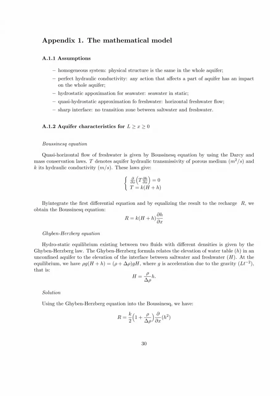
A.1.1 Assumptions
– homogeneous system: physical structure is the same in the whole aquifer;
– perfect hydraulic conductivity: any action that affects a part of aquifer has an impact
on the whole aquifer;
– hydrostatic appoximation for seawater: seawater in static;
– quasi-hydrostatic approximation fo freshwater: horizontal freshwater flow;
– sharp interface: no transition zone between saltwater and freshwater.
A.1.2 Aquifer characteristics for L ≥ x ≥ 0
Boussinesq equation
Quasi-horizontal flow of freshwater is given by Boussinesq equation by using the Darcy andmass conservation laws. T denotes aquifer hydraulic transmissivity of porous medium (m2/s) andk its hydraulic conductivity (m/s). These laws give:
{∂∂x
(T ∂h
∂x
)= 0
T = k(H + h)
By integrate the first differential equation and by equalizing the result to the recharge R, weobtain the Boussinesq equation:
R = k(H + h)∂h
∂x
Ghyben-Herzberg equation
Hydro-static equilibrium existing between two fluids with different densities is given by theGhyben-Herzberg law. The Ghyben-Herzberg formula relates the elevation of water table (h) in anunconfined aquifer to the elevation of the interface between saltwater and freshwater (H). At theequilibrium, we have ρg(H + h) = (ρ + ∆ρ)gH, where g is acceleration due to the gravity (Lt−2),that is:
H =ρ
∆ρh.
Solution
Using the Ghyben-Herzberg equation into the Boussinesq, we have:
R =k
2
(1 +
ρ
∆ρ
) ∂
∂x(h2)
30
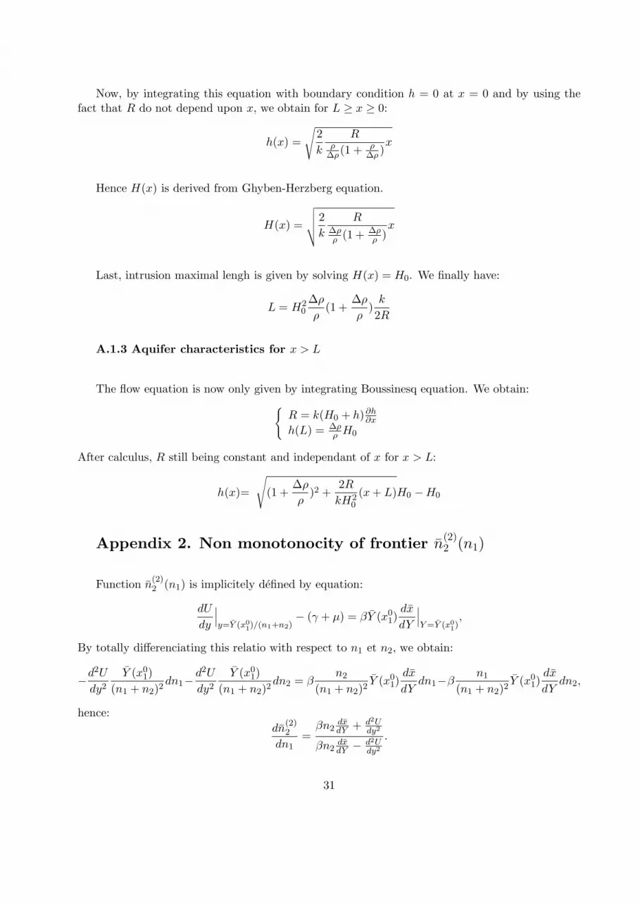
Now, by integrating this equation with boundary condition h = 0 at x = 0 and by using thefact that R do not depend upon x, we obtain for L ≥ x ≥ 0:
h(x) =
√2
k
Rρ
∆ρ(1 + ρ∆ρ )
x
Hence H(x) is derived from Ghyben-Herzberg equation.
H(x) =
√√√√2
k
R∆ρρ (1 + ∆ρ
ρ )x
Last, intrusion maximal lengh is given by solving H(x) = H0. We finally have:
L = H20∆ρ
ρ(1 +
∆ρ
ρ)
k
2R
A.1.3 Aquifer characteristics for x > L
The flow equation is now only given by integrating Boussinesq equation. We obtain:
{R = k(H0 + h)∂h
∂x
h(L) = ∆ρρ H0
After calculus, R still being constant and independant of x for x > L:
h(x) =
√(1 +
∆ρ
ρ)2 +
2R
kH20
(x + L)H0 −H0
Appendix 2. Non monotonocity of frontier n(2)2 (n1)
Function n(2)2 (n1) is implicitely defined by equation:
dU
dy
∣∣∣y=Y (x0
1)/(n1+n2)− (γ + µ) = βY (x0
1)dx
dY
∣∣∣Y =Y (x0
1),
By totally differenciating this relatio with respect to n1 et n2, we obtain:
−d2U
dy2
Y (x01)
(n1 + n2)2dn1−
d2U
dy2
Y (x01)
(n1 + n2)2dn2 = β
n2
(n1 + n2)2Y (x0
1)dx
dYdn1−β
n1
(n1 + n2)2Y (x0
1)dx
dYdn2,
hence:
dn(2)2
dn1=
βn2dxdY + d2U
dy2
βn2dxdY −
d2Udy2
.
31
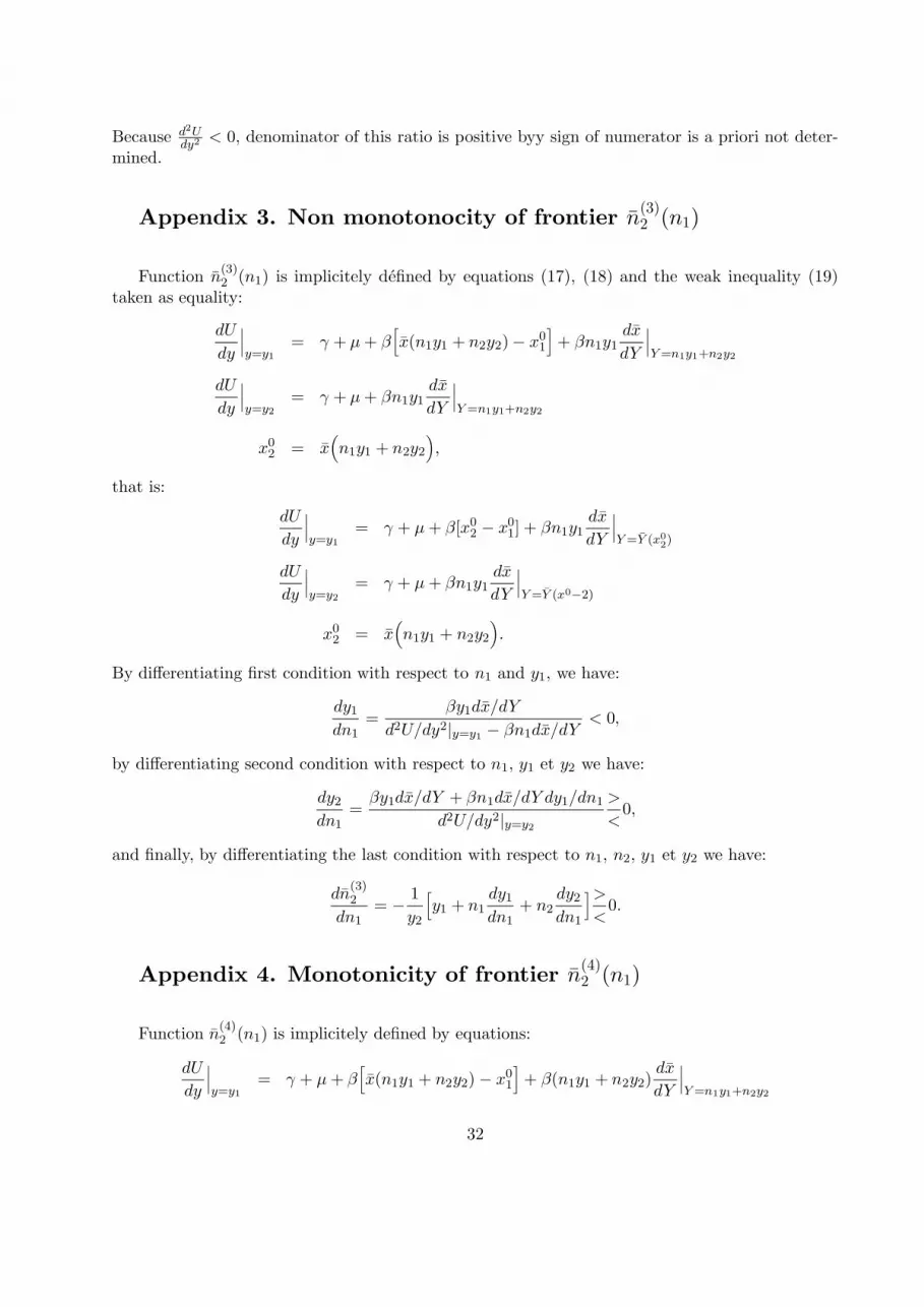
Because d2Udy2 < 0, denominator of this ratio is positive byy sign of numerator is a priori not deter-
mined.
Appendix 3. Non monotonocity of frontier n(3)2 (n1)
Function n(3)2 (n1) is implicitely defined by equations (17), (18) and the weak inequality (19)
taken as equality:
dU
dy
∣∣∣y=y1
= γ + µ + β[x(n1y1 + n2y2)− x0
1
]+ βn1y1
dx
dY
∣∣∣Y =n1y1+n2y2
dU
dy
∣∣∣y=y2
= γ + µ + βn1y1dx
dY
∣∣∣Y =n1y1+n2y2
x02 = x
(n1y1 + n2y2
),
that is:
dU
dy
∣∣∣y=y1
= γ + µ + β[x02 − x0
1] + βn1y1dx
dY
∣∣∣Y =Y (x0
2)
dU
dy
∣∣∣y=y2
= γ + µ + βn1y1dx
dY
∣∣∣Y =Y (x0−2)
x02 = x
(n1y1 + n2y2
).
By differentiating first condition with respect to n1 and y1, we have:
dy1
dn1=
βy1dx/dY
d2U/dy2|y=y1 − βn1dx/dY< 0,
by differentiating second condition with respect to n1, y1 et y2 we have:
dy2
dn1=
βy1dx/dY + βn1dx/dY dy1/dn1
d2U/dy2|y=y2
>
<0,
and finally, by differentiating the last condition with respect to n1, n2, y1 et y2 we have:
dn(3)2
dn1= −
1
y2
[y1 + n1
dy1
dn1+ n2
dy2
dn1
]>
<0.
Appendix 4. Monotonicity of frontier n(4)2 (n1)
Function n(4)2 (n1) is implicitely defined by equations:
dU
dy
∣∣∣y=y1
= γ + µ + β[x(n1y1 + n2y2)− x0
1
]+ β(n1y1 + n2y2)
dx
dY
∣∣∣Y =n1y1+n2y2
32
dU
dy
∣∣∣y=y2
= γ + µ + β(n1y1 + n2y2)dx
dY
∣∣∣Y =n1y1+n2y2
Y (x02) = n1y1 + n2y2,
that is:
dU
dy
∣∣∣y=y1
= γ + µ + β[x02 − x0
1] + βY (x02)
dx
dY
∣∣∣Y =Y (x0
2)
dU
dy
∣∣∣y=y2
= γ + µ + βY (x02)
dx
dY
∣∣∣Y =Y (x0−2)
Y (x02) = n1y1 + n2y2.
From the first equation we have:
y1 =dU
dy
−1[γ + µ + β[x0
2 − x01] + βY (x0
2)dx
dY
∣∣∣Y =Y (x0
2)
],
from the second, it follows:
y1 =dU
dy
−1[γ + µ + βY (x0
2)dx
dY
∣∣∣Y =Y (x0
2)
],
and by differentiating the last one with respect to n1, n2, y1 and y2 we finally obtain:
dn(4)2
dn1= −
y1
y2< −1
Appendix 5. Upper frontier of zone 2
Appendix 6. Upper frontier of zone 2i
Appendix 7. Upper frontier of zone 2i + 1
33
.
Figure 1 : Coastal aquifer under natural equilibrium
Figure 2 : Aquifer optimal use by a single agglomeration(1) Low population size.
(2) Intermediate population size.(3) Important population size.
34
.
F igure 3 : Zoning in population sizes space
Curve (2) represents functionn(2)2 (n1),
Curve (3) represents functionn(3)2 (n1),
Curve (4) represents functionn(4)2 (n1).
F igure 4 : Impossible frontier for zone II
35
.
Figure 5 : Per capita water consumptionfor 2 agglomeration case alonga line (n1, n2) = (n1, αn1), α > 0
Figure 6 : Per capita water consumptionfor 4 agglomerations case alonga line(n1, n2, n3, n4) = (n1, α2n1, α3n1, α4n1)
NB. On a: y(7)3+ = y
(7)4 et y
(8)3+ = y
(8)4
36

Figure1
R
x
z
L
MILIEU IMPERMEABLE
−H0
X 0
MILIEU POREUX
Sol
Mer
EauSalée
Aquifère
EauDouce
h x( )− H x( )
00
Figure 2
Y
γ µ+
Y ( )1 Y Y( )2 0= Y ( )3
( )1 ( )2 ( )3 ( )γ µ β β+ + − +x Y x Y dx dY( ) 0
0
′V Y
C Ym
( )
( )
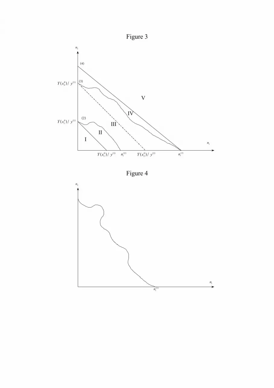
Figure 3
Y x y( )/ ( )10 1
Y x y( )/ ( )10 1
Y x y( )/ ( )20 1
Y x y( )/ ( )20 1n1
2( ) n13( )
n1
n2
III
III
IV
V
( )2
( )3
( )4
Figure 4
n12( )
n2
n1
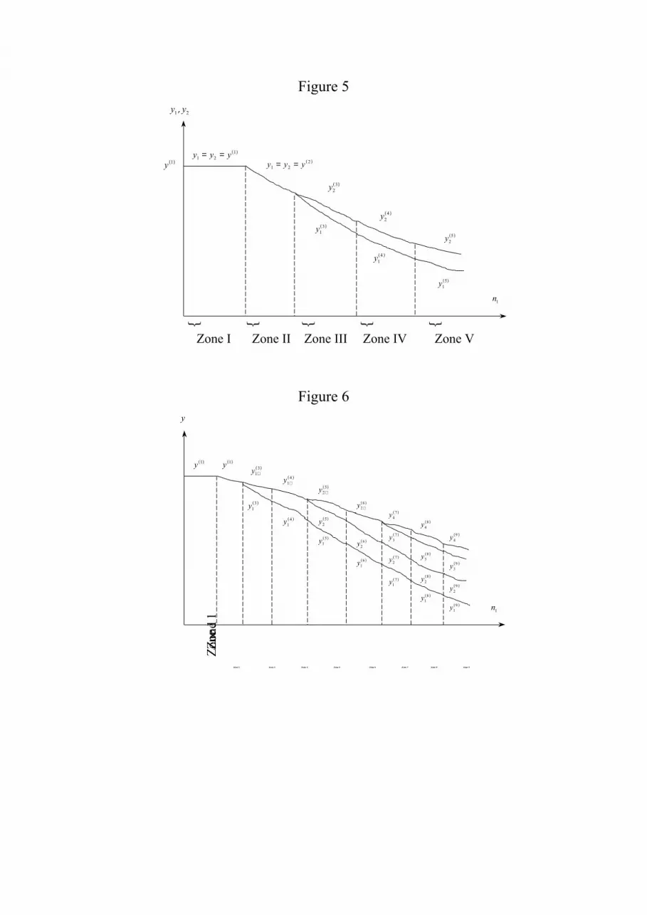
Figure 5
{ { { { n1
Zone I Zone II Zone III Zone IV Zone V
{
y y1 2,
y( )1y y y1 2
1= = ( )
y y y1 22= = ( )
y23( )
y13( )
y24( )
y14( )
y25( )
y15( )
Figure 6
n1
Zon
e 1
y
y ( )1
Zone 2 Zone 3 Zone 4 Zone 5 Zone 6 Zone 7 Zone 8 Zone 9
y ( )1
y13+
( )
y14+
( )
y25+
( )
y26+
( )
y47( )
y48( )
y49( )
y13( )
y14( )
y15( )
y16( )
y17( )
y18( )
y19( )
y25( )
y26( )
y27( )
y37( )
y28( )
y38( )
y29( )
y39( )