estimation of viral infection and replication in cells by using convolution models

Journal compilation © 2010 Royal Statistical Society 0035–9254/10/59423No claim to original US Government works

Appl. Statist. (2010)59, Part 3, pp. 423–435

Estimation of viral infection and replication in cellsby using convolution models

Dean Follmann, Jing Qin and Yo Hoshino

National Institute of Allergy and Infectious Diseases, Bethesda, USA

[Received February 2009. Revised September 2009]

Summary. In some assays, a diluted suspension of infected cells is plated onto multiple wells.In each well the number of genome copies of virus, Y , is recorded, but interest focuses on thenumber of infected cells, X , and the number of genome copies in the infected cells, W1; . . . ; WX .The statistical problem is to recover the distribution or at least moments of X and W on thebasis of the convolution Y. We evaluate various parametric statistical models for this ‘mixture’-type problem and settle on a flexible robust approach where X follows a two-component Poissonmixture model and W is a shifted negative binomial distribution. Data analysis and simulationsreveal that the means and occasionally variances of X and W can be reliably captured bythe model proposed. We also identify the importance of selecting an appropriate dilution for areliable assay.

Keywords: Assays; Deconvolution; Mixture model; Robust methods; Stopped sum

1. Introduction

Herpes simplex virus type 2 (HSV 2) causes a lifelong infection that is characterized by latencypunctuated by occasional reactivation events. The initial or primary infection, which is generallycaused by sexual contact with an infected partner, is characterized by rapid replication in themucosa and the development of genital lesions. Initial infections can be severe, but the immunesystem generally controls primary infection leading to a latent infection where some nerve cellscontain copies of the virus genome. Although the total latent viral load is known to be correlatedwith reactivation rates in animal models (Hoshino et al., 2007), the distribution of virus genomewithin and between nerve cells is incompletely understood. For example, O’Neil et al. (2004)showed that the latent viral load in ganglia is independent of the size of the infectious dose inrabbits, whereas others have shown the opposite.

The latent viral load is actually the sum over the number of infected cells of the number ofvirions in each cell. Thus a latent viral load may be large because many cells are infected eachwith a modest number of viruses, or because a few infected cells have a large number of viruses.Knowledge of the contribution of each is important to help to understand the virus’s life cycleand also may have consequences for drug development. For example, if only a few cells tendto become infected, but some fraction of those do have explosive replication, drugs that targetwithin-cell replication may be more promising than drugs that focus on preventing cell infection.

To help to understand latent HSV 2 infection, a novel experiment was performed. ChallengeHSV 2 was introduced into both eyes of experimental mice. Following establishment of a latent

Address for correspondence: Dean Follmann, Biostatistics Research Branch, National Institute of Allergy andInfectious Diseases, 6700A Rockledge Drive, Bethesda, MD 20892-7609, USA.E-mail: [email protected]

424 D. Follmann, J. Qin and Y. Hoshino

infection in the trigeminal ganglia (the mass of neural tissue that is connected to each eye),mice were sacrificed and the two trigeminal ganglia were dispersed into single-cell suspensionand placed into an 88-well plate. From each well, realtime polymerase chain reaction was usedto determine the number of HSV 2 genome copies, say Y. Letting X be the number of infectedcells and W1, . . . , WX the number of genome copies of virus in each infected cell, then Y =W1 + . . . +WX. The statistical problem is to establish the distributions of both X and Wi, or atleast some moments, on the basis of only Y. Thus Y is a convolution and our goal is to deconvolveor to estimate the constituent distributions when X , W1, . . . , WX and Y are all integers.

A related problem has been discussed by others including Kendall (1974) and Ninan et al.(2006). Under their formulation, the real number W = V + " where " has a mean 0 symmetricdistribution with continuous support and relatively small variance. Then a random number Xof these W s are summed to produce Y. Both Kendall (1974) and Ninan et al. (2006) applied anestimating equation approach to estimate E.W/=E.V/. Although appealingly non-parametric,their approach is not suited for our setting with integer W , possibly large variability and nodecomposition of W into V +". For parametric approaches to the W =V +" problem, see Ryanet al. (1997) and Aravanis et al. (2003).

This paper is organized as follows. We begin by introducing notation and giving an expandeddiscussion of the experimental assay. We then postulate parametric models for the data wherethe number of infected cells per well (X ) follows a Poisson or negative binomial distribution andthe number of genome copies per infected cell (W ) follows a shifted Poisson or shifted negativebinomial distribution. We also allow X to follow a discrete mixture of two Poisson distributionsas a way to address potential outliers, following an approach of Follmann and Lambert (1989).An important use of the models is to aid in the design of the assay, in particular the amountof dilution that should be used. We discuss how different choices impact the variance of themaximim likelihood estimators (MLEs) and show that dilution where about 25% of the wellshave Y =0 works well. The behaviour of the models is investigated by simulation and the modelsare applied to two mouse experiments that highlight practical issues that are involved in theiruse.

The data that are analysed in the paper can be obtained from

http://www.blackwellpublishing.com/rss

2. Background and models

We first describe the cell infection process and the assay. To start, assume that free virus existsin the host (e.g. humans). This free virus needs to infect host cells to complete a stage of itslife cycle. First a virion attaches onto a cell and then gains entry through the cell membrane bybinding of specific viral and cellular receptor molecules. Once in the cell, the virion eventuallyreplicates a number of times, producing multiple genome copies that lie within the cell. A cellmight be infected with multiple virions, called superinfection, where each virion initiates itsown sequence of replication events. A cell might stay thus infected for an indefinite period oftime. However, any successful virus will eventually burst forth from the cell, engaging in thenext stage of its life which ultimately entails movement to another host, completing the cycle.In deciphering the life cycle of any virus, different aspects are of interest including how manycells are typically infected and how much replication occurs within an infected cell.

A brief description of an experiment that was designed to address these issues for HSV 2follows. 9–10-week-old C57BlL/6 and DBA2 mice were challenged with HSV 2 on both oftheir corneas (Hoshino et al., 2008). This ensured infection of some nerve cells associated witheach eye. Different mice received different challenge doses (or inocula) of virus. 28 days after

Estimation of Viral Infection and Replication 425

challenge the mice were sacrificed and the trigeminal ganglia or collection of nerve cells thatare associated with each eye were harvested and suspended in solution. The solution was thendiluted and placed into the 88 wells of a single plate. Let X denote the number of infected cellsin a well, and let Y denote the number of genome copies of virus that are detected in a well.Finally, let Wi denote the number of genome copies in the ith infected cell in a well, i=1, . . . , X.Note that Y =0 if X=0. Thus Y and X can take values 0, 1, . . . , whereas Wi takes values 1, 2, . . . ,and

Y =W1 +W2 + . . . +WX:

Owing to superinfection, or the infection of a cell by multiple virions, X counts the numberof cells that have been infected by at least one virion and Wi is thus based on the replicationprocesses of at least one infecting virion. Note that the chance of superinfection is related to thesize of the inoculum, or natural virus in the host, rather than by the number of infected cells perwell, whose distribution is strongly influenced by dilution.

Probabilistically, one can think of a large urn (a soup of trigeminal ganglia) composed of anumber X of red (infected neurons) and black (uninfected neurons) balls. Each of the red ballshas a positive integer W written on it. On 88 occasions a scoop is used to extract a number ofballs from the urn, but only the sum of the red integers from each scoop (Y ) is recorded beforediscarding. We can represent the distribution of Y as

P.Y =0/=P.X=0/,

P.Y =y/=y∑

j=1P.W+j =y|X= j/P.X= j/

for y=1, 2, . . . where W+j =W1 +W2 + . . . +Wj. This type of distribution is known as a ‘stoppedsum’ distribution; the summing on j stops at X. See Johnson et al. (2005) for an extensivediscussion.

If W is point mass at 1 we have P.Y = y/ = P.X = y/. Thus we cannot estimate X and Wnon-parametrically on the basis of Y alone and restrictions need to be placed on the distribu-tions of X and W+X to ensure identifiability. From the physical description of the problem asballs in an urn, a natural initial model for X is Poisson with parameter λ. To aid in specifyingthe distribution of W+X recall that the viral replication process that unfolds in each infectedcell occurs before segregation into a well. Thus we shall assume that the distribution of the(future) wellmate counts W1, . . . , WX is independent and identically distributed. Since we workwith W+X it is very appealing to consider models for the Wis that are closed under convolutionsuch as the Poisson or negative binomial distributions. However, we need to address a slightcomplication first. By definition, Wi �1 since it is the number of virions in an infected cell. Weshall thus work with WÅ

i =Wi −1 where WÅi follows a Poisson or negative binomial distribution,

and we shall say that Wi follows a shifted Poisson or shifted negative binomial model. Usingthis representation we can write Y =X+WÅ+X and thus

P.Y =0/=P.X=0/, .1/

P.Y =y/=y∑

j=1P.WÅ

+j =y − j|X= j/ P.X= j/, .2/

for y =1, 2, . . . .If we assume that WÅ

i is Poisson distributed with parameter θ then WÅ+X is Poisson.Xθ/.Suppose that WÅ

i is negative binomial distributed with mean and variance {αβ, α.1 + β/};


then WÅ+X is negative binomial with parameters .Xαβ, Xα.1 + β//. This parameterization ofthe negative binomial distribution can be derived by postulating that, given a parameter ω,WÅ

i is Poisson(ω) but that ω follows a gamma distribution with mean and variance .αβ, αβ2/.Substituting these parametric models into equation (2) we obtain the Poisson–negative binomial(P–NB) model

P.Y =y/=y∑

j=1

Γ{.y − j/+ jα}Γ{.y − j/+1} Γ.jα/

(β

β +1

)y−j (1

β +1

)jα

P.X= j/, .3/

for y > 0 with P.Y = 0/ = P.X = 0/ = exp.−λ/ and where P.X = j/ is the Poisson probabilitymass function. The Poisson–Poisson (P–P) model is similar. The unshifted versions of the P–Pand P–NB models are discussed in Johnson et al. (2005) and are called respectively the Neymantype A and Poisson–Pascal distribution. The Poisson–shifted Poisson distribution is known asthe Thomas distribution.

In the preparation of the trigeminal ganglion mass into a suspension, collagenase is used tohelp to separate the mass into free-floating individual neurons. However, the collagenase maywork incompletely, resulting in a tangled collection of neurons that travel together into a well.Thus although the Poisson model for X makes sense on theoretical grounds for an ideal assay,in practice clumping may lead to greater variability in X than allowed for by a Poisson model.We might imagine that the number of clumps follow a Poisson distribution, but the number ofinfected cells per clump follow a different distribution F. If F follows a logarithmic distribution,then X follows a negative binomial distribution (Johnson et al., 2005). When this distributionfor X in equation (3) is coupled with a negative binomial distribution for W we obtain thenegative binomial–negative binomial (NB–NB) model.

Finally, a different model for X can be developed from robustness considerations. Follmannand Lambert (1989) demonstrated that a discrete mixture of logistic regression models hadsome robust properties, compared with an unmixed logistic regression model. Loosely, we mightimagine that, with probability p, X follows the ‘typical’ Poisson.λ1/ distribution; otherwise itfollows an ‘aberrant’ Poisson.λ2) distribution. We call this the mixed Poisson distribution. Inequation (3) we have P.X = j/ = P.X = j;λ1/p + P.X = j;λ2/.1 − p/, where P.X = j;λ/ is thePoisson probability mass function.

Thus in total we shall consider five different models for X–WÅ: the P–P, P–NB, mixed Poisson–Poisson (MP–P), mixed Poisson–negative binomial (MP–NB) and finally the NB–NB model.These have respectively, two, three, three, five and four parameters.

3. Estimation and model evaluation

Maximum likelihood estimation is used to estimate the parameters of the model. In constructingthe likelihood we need to address the interval censoring of realtime polymerase chain reaction.Whereas Y =0 is observed correctly, values of Y from 1 to 4 are unreliable. This induces intervalcensoring and associated log-likelihood

l.η/=n∑

i=1− log{P.Y =0;η/}I.yi =0/+ I.1�yi �4/ log{P.1�Y �4;η/}

+ I.yi > 4/ log{P.Y =yi;η/}where η is a vector of parameters for the model. To obtain confidence intervals for parameters ofinterest, we use the method of profile likelihood. Suppose that we decompose η= .θ, ω/, whereθ is the parameter of interest. We form the profile log-likelihood


h.θ/=2[l.η/− l{θ, ω.θ/}],

where η is the MLE of η and ω.θ/ the MLE of ω at a fixed value of θ. To construct an approximate95% confidence interval we find θL < θU so that h.θZ/ = 3:84 for Z = U, L (Cox and Hinkley,1974).

In practice, the different models may produce different inferences and we shall want to knowwhich model is best. Informally, Q–Q-plots and comparison of sample with theoretical momentscan be used. More formally, we can compare log-likelihoods. This is not straightforward in oursetting. Minus twice the difference in log-likelihood has an asymptotic null χ2-distribution fornested models with parameters on the interior of the parameter space (Cox and Hinkley, 1974).The comparison of MP–NB versus NB–NB models is not nested whereas all other comparisonsare on the boundary of the parameter space with either var.WÅ/ or var.X/ equal to 0. For theboundary problem setting it is generally true that the null distribution is an equal mixture ofpoint mass at 0 and a χ2-distribution with 1 degree of freedom (see for example Self and Liang(1987)). Thus a α<0:50 level procedure obtains by using a critical value c satisfying P.χ>c/=2αwhere χ is a χ2 random variable with 1 degree of freedom.

For the non-nested model problem, Cox (1961, 1962) suggested that comparing log-likelihoods can still be useful. We could set as the null hypothesis that the data follow a four-parameter NB–NB model, say HN

0 , and have as the alternative hypothesis the five-parameterMP–NB model, say HM

A . For such a formulation, Cox suggested the use of the difference inlog-likelihoods, shifted to have mean 0 on HN

0 :

T.N, M/= lN.ηN/− lM.ηM/−EN{lN.ηN/− lM.ηM/}

where N and ηN denote the NB–NB model and parameters, and M and ηM denote the MP–NB model and parameters. The notation EN.·/ denotes the expectation under the assumptionof the NB–NB model evaluated at the MLEs. If the MP–NB model is correct, then T (N ,M)should be negative. A simulated null distribution can be used to determine an approximate nulldistribution for T (N ,M) (see Williams (1970) and Hinde (1992)). Using the estimated ηN in theNB–NB model, generate B statistics T Å

1 .N, M/, . . . , T ÅB .N, M/. Then an approximate p-value is

[#{T Åi .N, B/�T.N, B/}+1]=.B+1/. If this p-value is small, it suggests that the MP–NB model

is superior to the NB–NB model. One can also switch the null and alternative hypotheses anduse the procedure that was described above using T (M, N) rather than T (N, M) to see whetherthe NB–NB model is superior to the MP–NB model.

4. Data analysis

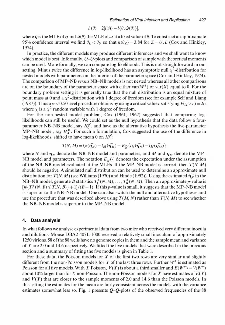
In what follows we analyse experimental data from two mice who received very different inoculaand dilutions. Mouse DBA2-407L-1000 received a relatively small inoculum of approximately1250 virions. 58 of the 88 wells have no genome copies in them and the sample mean and varianceof Y are 2.0 and 14.6 respectively. We fitted the five models that were described in the previoussection and a summary of fitting the five models is given in Table 1.

For these data, the Poisson models for X of the first two rows are very similar and slightlydifferent from the non-Poisson models for X of the last three rows. Further WÅ is estimated asPoisson for all five models. With X Poisson, V (X ) is about a third smaller and E.WÅ/=V.WÅ/

about 10% larger than for X non-Poisson. The non-Poisson models for X have estimates of E(Y )and V (Y ) that are closer to the sample moments of 2.0 and 14.6 than the Poisson models. Inthis setting the estimates for the mean are fairly consistent across the models with the varianceestimates somewhat less so. Fig. 1 presents Q–Q-plots of the observed frequencies of the 88


Table 1. Parameter estimates for fitted models based on the 88 wells from mouseDBA2-407L-1000†

X –W −l E(X) V (X) E(WÅ) V (WÅ) E(Y ) V (Y)

P–P 118.5 0.40 0.40 4.07 4.07 2.02 11.89(0.3,0.6) (0.3,0.6) (3.2,5.1) (3.2,5.1)

P–NB 118.5 0.40 0.40 4.07 4.07 2.02 11.89(0.3,0.6) (0.3,0.6) (3.2,5.6) (3.2,14.7)

MP–P 117.6 0.44 0.61 3.64 3.64 2.02 14.84(0.3,0.7) (0,1.8) (2.5,4.8) (2.5,4.8)

MP–NB 117.6 0.44 0.61 3.63 3.63 2.03 14.73(0.3,0.5) (0,1.6) (2.5,4.1) (2.6,10.4)

NB–NB 117.9 0.45 0.63 3.48 3.48 2.01 14.16(0.3,0.7) (0.3,1.8) (2.5,5.1) (2.5,10.7)

†The MLEs are reported along with 95% profile likelihood confidence intervals. Thesample mean and variance of Y are 2.0 and 14.6 respectively.

0 5 10 15 20

0

5

10

15

20

Well Counts(a)

(b)

0 5 10 15 20

0

5

10

15

20

Well Counts

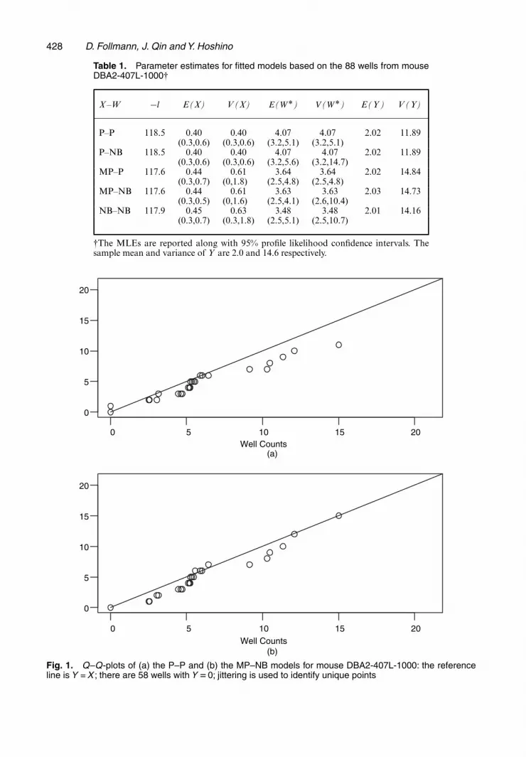
Fig. 1. Q–Q-plots of (a) the P–P and (b) the MP–NB models for mouse DBA2-407L-1000: the referenceline is Y = X ; there are 58 wells with Y D0; jittering is used to identify unique points


counts compared with the P–P and MP–P models, indicating a somewhat better fit for theMP–P model. The Q–Q-plot for the NB–P model is similar (the figure is not shown). In pickinga single model, either the NB–P or MP–P model seems reasonable.

The second mouse, DBA2-433L-1600, received an inoculum of 160000, which was over100-fold greater than for the first mouse, resulting in an enormously high latent viral load.In addition, the dilution of suspension is such that only one of the 88 wells has no genomecopies in it. The sample mean and variance of Y are respectively 137 and 21691. This massiveinoculum was selected as the assay was being developed and would not be used in future;nonetheless we report it here to illustrate the performance of the proposed models under anextreme condition.

A summary of the five model fits is given in Table 2. On the basis of the log-likelihood we seesubstantial improvement in all models relative to the simple P–P model, which underpredictsthe variance of Y by about a factor of 4. Going down the rows we see that both the P–NBand the MP–P models allow for greater heterogeneity, but the models respectively assume thatit comes either from extra-Poisson variability in the within-cell replication process, or fromextra-Poisson variability in the number of infected cells. The likelihood is indifferent betweenthese two models and they reach similar conclusions about E(X ) and E(W ) but substantiallydifferent conclusions about V (X ) and V (W ): (6.3, 1339.7) for the P–NB model and (24.6, 25.2)for the MP–P model. The MP–NB model (fourth row) has a much larger likelihood with esti-mates of E(X ) and E.WÅ/ similar to those from the P–NB and MP–P models, but dissimilarestimates of V (X ) and V.WÅ/. The NB–NB (fifth row) model has an appreciably worse likeli-hood than the MP–NB model and a substantially different conclusion from all other modelsabout E(X ) and E.WÅ/. For the NB–NB model the mean of E(X ) is about twice that of E.WÅ/

whereas for all other models E(X ) is a seventh to a quarter that of E.WÅ/. Additionally, theconfidence intervals for E(X ) and V (X ) with the NB–NB model are very wide.

Using Cox’s method to test HN0 versus HM

A obtains a simulated p-value of 0.028, based on1000 simulations of the null distribution, which also suggests the superiority of the MP–NBmodel. Testing the null hypothesis of an MP–NB model or HM

0 versus an alternative of anNB–NB model or HN

A obtains a simulated p-value of 0.11, providing not much evidence thatthe NB–NB model is superior to the MP–NB model.

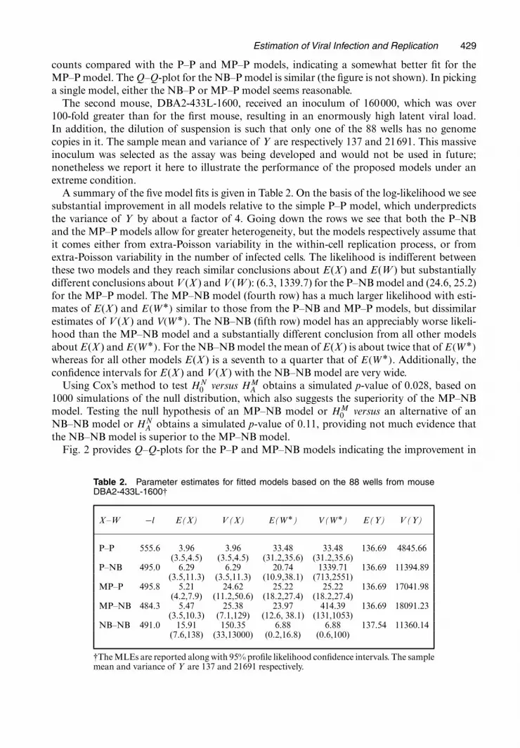
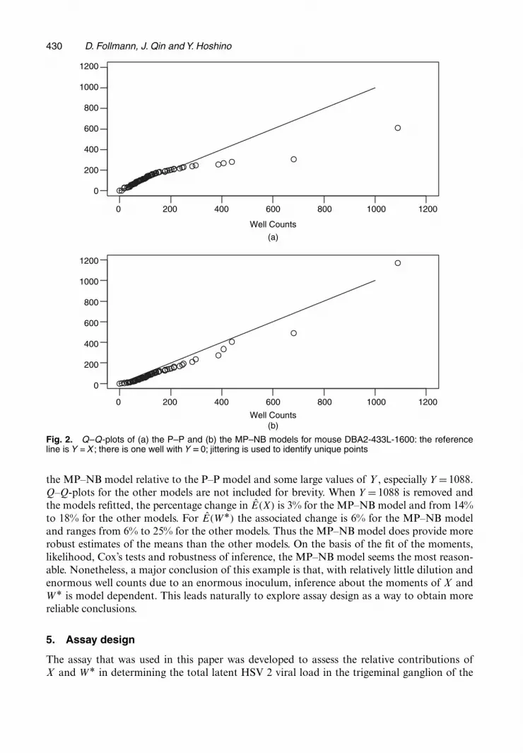
Fig. 2 provides Q–Q-plots for the P–P and MP–NB models indicating the improvement in

Table 2. Parameter estimates for fitted models based on the 88 wells from mouseDBA2-433L-1600†

X –W −l E(X) V (X) E(WÅ) V (WÅ) E(Y) V (Y)

P–P 555.6 3.96 3.96 33.48 33.48 136.69 4845.66(3.5,4.5) (3.5,4.5) (31.2,35.6) (31.2,35.6)

P–NB 495.0 6.29 6.29 20.74 1339.71 136.69 11394.89(3.5,11.3) (3.5,11.3) (10.9,38.1) (713,2551)

MP–P 495.8 5.21 24.62 25.22 25.22 136.69 17041.98(4.2,7.9) (11.2,50.6) (18.2,27.4) (18.2,27.4)

MP–NB 484.3 5.47 25.38 23.97 414.39 136.69 18091.23(3.5,10.3) (7.1,129) (12.6, 38.1) (131,1053)

NB–NB 491.0 15.91 150.35 6.88 6.88 137.54 11360.14(7.6,138) (33,13000) (0.2,16.8) (0.6,100)

†The MLEs are reported along with 95% profile likelihood confidence intervals. The samplemean and variance of Y are 137 and 21691 respectively.


0 200 400 600 800 1000 1200

0

200

400

600

800

1000

1200

Well Counts

(a)

(b)

0 200 400 600 800 1000 1200

0

200

400

600

800

1000

1200

Well Counts

Fig. 2. Q–Q-plots of (a) the P–P and (b) the MP–NB models for mouse DBA2-433L-1600: the referenceline is Y = X ; there is one well with Y D0; jittering is used to identify unique points

the MP–NB model relative to the P–P model and some large values of Y , especially Y =1088.Q–Q-plots for the other models are not included for brevity. When Y = 1088 is removed andthe models refitted, the percentage change in E.X/ is 3% for the MP–NB model and from 14%to 18% for the other models. For E.WÅ/ the associated change is 6% for the MP–NB modeland ranges from 6% to 25% for the other models. Thus the MP–NB model does provide morerobust estimates of the means than the other models. On the basis of the fit of the moments,likelihood, Cox’s tests and robustness of inference, the MP–NB model seems the most reason-able. Nonetheless, a major conclusion of this example is that, with relatively little dilution andenormous well counts due to an enormous inoculum, inference about the moments of X andWÅ is model dependent. This leads naturally to explore assay design as a way to obtain morereliable conclusions.

5. Assay design

The assay that was used in this paper was developed to assess the relative contributions ofX and WÅ in determining the total latent HSV 2 viral load in the trigeminal ganglion of the


mouse. In principle it could be applied more generally, using different viruses, different routes ofadminstration and different hosts. It could also be applied to study natural viral pathogenesis.In general, it is clear that the performance of the assay is affected by at least three factors: thenumber of replicates, dilution and, when relevant, the size of inoculum. Indeed in our selectedmouse experiments we saw consistent results with a small inoculum and substantial dilution butinconsistent results with a large inoculum, enormous well counts and little dilution.

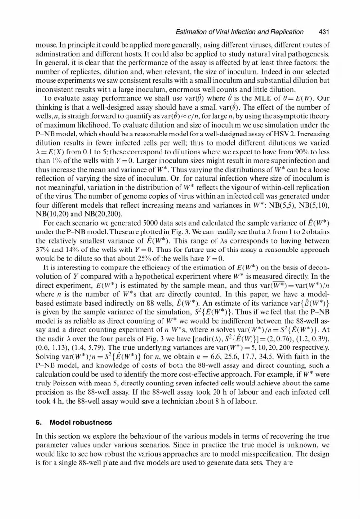
To evaluate assay performance we shall use var.θ/ where θ is the MLE of θ = E.W/. Ourthinking is that a well-designed assay should have a small var.θ/. The effect of the number ofwells, n, is straightforward to quantify as var.θ/≈c=n, for large n, by using the asymptotic theoryof maximum likelihood. To evaluate dilution and size of inoculum we use simulation under theP–NB model, which should be a reasonable model for a well-designed assay of HSV 2. Increasingdilution results in fewer infected cells per well; thus to model different dilutions we variedλ=E.X/ from 0.1 to 5; these correspond to dilutions where we expect to have from 90% to lessthan 1% of the wells with Y =0. Larger inoculum sizes might result in more superinfection andthus increase the mean and variance of WÅ. Thus varying the distributions of WÅ can be a loosereflection of varying the size of inoculum. Or, for natural infection where size of inoculum isnot meaningful, variation in the distribution of WÅ reflects the vigour of within-cell replicationof the virus. The number of genome copies of virus within an infected cell was generated underfour different models that reflect increasing means and variances in WÅ: NB(5,5), NB(5,10),NB(10,20) and NB(20,200).

For each scenario we generated 5000 data sets and calculated the sample variance of E.WÅ/

under the P–NB model. These are plotted in Fig. 3. We can readily see that a λ from 1 to 2 obtainsthe relatively smallest variance of E.WÅ/. This range of λs corresponds to having between37% and 14% of the wells with Y = 0. Thus for future use of this assay a reasonable approachwould be to dilute so that about 25% of the wells have Y =0.

It is interesting to compare the efficiency of the estimation of E.WÅ/ on the basis of decon-volution of Y compared with a hypothetical experiment where WÅ is measured directly. In thedirect experiment, E.WÅ/ is estimated by the sample mean, and thus var.WÅ/ = var.WÅ/=n

where n is the number of WÅs that are directly counted. In this paper, we have a model-based estimate based indirectly on 88 wells, E.WÅ/. An estimate of its variance var{E.WÅ/}is given by the sample variance of the simulation, S2{E.WÅ/}. Thus if we feel that the P–NBmodel is as reliable as direct counting of WÅ we would be indifferent between the 88-well as-say and a direct counting experiment of n WÅs, where n solves var.WÅ/=n = S2{E.WÅ/}. Atthe nadir λ over the four panels of Fig. 3 we have [nadir.λ/, S2{E.W/}] = .2, 0:76/, (1.2, 0.39),(0.6, 1.13), (1.4, 5.79). The true underlying variances are var.WÅ/ = 5, 10, 20, 200 respectively.Solving var.WÅ/=n = S2{E.WÅ/} for n, we obtain n = 6.6, 25.6, 17.7, 34.5. With faith in theP–NB model, and knowledge of costs of both the 88-well assay and direct counting, such acalculation could be used to identify the more cost-effective approach. For example, if WÅ weretruly Poisson with mean 5, directly counting seven infected cells would achieve about the sameprecision as the 88-well assay. If the 88-well assay took 20 h of labour and each infected celltook 4 h, the 88-well assay would save a technician about 8 h of labour.

6. Model robustness

In this section we explore the behaviour of the various models in terms of recovering the trueparameter values under various scenarios. Since in practice the true model is unknown, wewould like to see how robust the various approaches are to model misspecification. The designis for a single 88-well plate and five models are used to generate data sets. They are


1

2

3

4

5

6

lambda

S^2

of e

st. E

(W*)

0.5

1.0

1.5

2.0

lambda

S^2

of e

st. E

(W*)

2

4

6

8

lambda

S^2

of e

st. E

(W*)

1 2 3 4 5 1 2 3 4 5

1 2 3 4 5 1 2 3 4 5

10

20

30

40

lambda

(a) (b)

(c) (d)

S^2

of e

st. E

(W*)

Fig. 3. Plots of the sample variance of E .W / under the P–NB model from data generated under a P–NBmodel (the Poisson parameter λ reflects the dilution of the assay whereas the negative binomial W Å reflectsthe extent of within-cell viral replication; each dot is based on 5000 simulated assays; �, nadir—the optionaldilution for estimating E.W Å/): (a) W Å � NB(5, 5); (b) W Å � NB(5, 10); (c) W Å � NB(10, 20); (d) W Å � NB(20, 200)

(a) X∼ Poisson(1) and WÅ ∼ Poisson(5),(b) X∼ Poisson(1) and WÅ ∼NB.α=10, β =1/,(c) X∼0:8 Poisson(1) + 0:2 Poisson(10) and WÅ ∼ Poisson(5),(d) X∼0:8 Poisson(1) + 0:2 Poisson(10) and WÅ ∼NB.α=1, β =1/ and(e) X∼NB.α=1, β =1/ and WÅ ∼NB.α=10, β =1/.

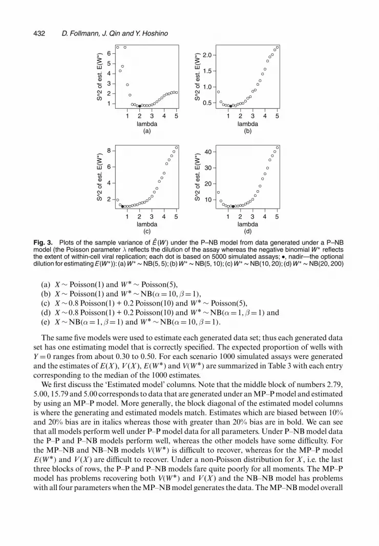
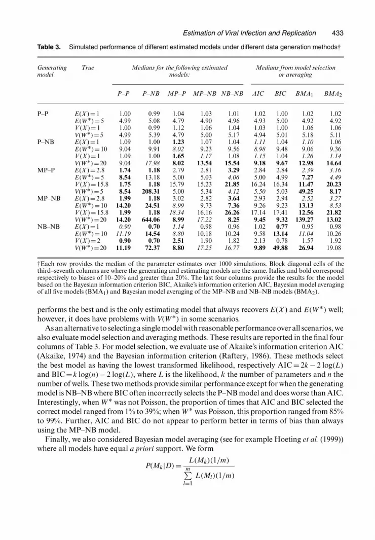
The same five models were used to estimate each generated data set; thus each generated dataset has one estimating model that is correctly specified. The expected proportion of wells withY =0 ranges from about 0.30 to 0.50. For each scenario 1000 simulated assays were generatedand the estimates of E(X ), V (X ), E.WÅ/ and V.WÅ/ are summarized in Table 3 with each entrycorresponding to the median of the 1000 estimates.

We first discuss the ‘Estimated model’ columns. Note that the middle block of numbers 2.79,5.00, 15.79 and 5.00 corresponds to data that are generated under an MP–P model and estimatedby using an MP–P model. More generally, the block diagonal of the estimated model columnsis where the generating and estimated models match. Estimates which are biased between 10%and 20% bias are in italics whereas those with greater than 20% bias are in bold. We can seethat all models perform well under P–P model data for all parameters. Under P–NB model datathe P–P and P–NB models perform well, whereas the other models have some difficulty. Forthe MP–NB and NB–NB models V.WÅ/ is difficult to recover, whereas for the MP–P modelE.WÅ/ and V (X ) are difficult to recover. Under a non-Poisson distribution for X , i.e. the lastthree blocks of rows, the P–P and P–NB models fare quite poorly for all moments. The MP–Pmodel has problems recovering both V.WÅ/ and V (X ) and the NB–NB model has problemswith all four parameters when the MP–NB model generates the data. The MP–NB model overall


Table 3. Simulated performance of different estimated models under different data generation methods†

Generating True Medians for the following estimated Medians from model selectionmodel models: or averaging

P–P P–NB MP–P MP–NB NB–NB AIC BIC BMA1 BMA2

P–P E(X ) = 1 1.00 0.99 1.04 1.03 1.01 1.02 1.00 1.02 1.02E.WÅ/=5 4.99 5.08 4.79 4.90 4.96 4.93 5.00 4.92 4.92V (X ) = 1 1.00 0.99 1.12 1.06 1.04 1.03 1.00 1.06 1.06V.WÅ/=5 4.99 5.39 4.79 5.00 5.17 4.94 5.01 5.18 5.11

P–NB E(X ) =1 1.09 1.00 1.23 1.07 1.04 1.11 1.04 1.10 1.06E.WÅ/=10 9.04 9.91 8.02 9.23 9.56 8.98 9.48 9.06 9.36V (X ) = 1 1.09 1.00 1.65 1.17 1.08 1.15 1.04 1.26 1.14V.WÅ/=20 9.04 17.98 8.02 13.54 15.54 9.18 9.67 12.98 14.64

MP–P E(X ) = 2.8 1.74 1.18 2.79 2.81 3.29 2.84 2.84 2.39 3.16E.WÅ/=5 8.54 13.18 5.00 5.03 4.06 5.00 4.99 7.27 4.49V (X ) = 15.8 1.75 1.18 15.79 15.23 21.85 16.24 16.34 11.47 20.23V.WÅ/=5 8.54 208.31 5.00 5.34 4.12 5.50 5.03 49.25 8.17

MP–NB E(X ) = 2.8 1.99 1.18 3.02 2.82 3.64 2.93 2.94 2.52 3.27E.WÅ/=10 14.20 24.51 8.99 9.73 7.36 9.26 9.23 13.13 8.53V (X ) = 15.8 1.99 1.18 18.34 16.16 26.26 17.14 17.41 12.56 21.82V.WÅ/=20 14.20 644.06 8.99 17.22 8.25 9.45 9.32 139.27 13.02

NB–NB E(X ) =1 0.90 0.70 1.14 0.98 0.96 1.02 0.77 0.95 0.98E.WÅ/=10 11.19 14.54 8.80 10.18 10.24 9.58 13.14 11.04 10.26V (X ) = 2 0.90 0.70 2.51 1.90 1.82 2.13 0.78 1.57 1.92V.WÅ/=20 11.19 72.37 8.80 17.25 16.77 9.89 49.88 26.94 19.08

†Each row provides the median of the parameter estimates over 1000 simulations. Block diagonal cells of thethird–seventh columns are where the generating and estimating models are the same. Italics and bold correspondrespectively to biases of 10–20% and greater than 20%. The last four columns provide the results for the modelbased on the Bayesian information criterion BIC, Akaike’s information criterion AIC, Bayesian model averagingof all five models (BMA1) and Bayesian model averaging of the MP–NB and NB–NB models (BMA2).

performs the best and is the only estimating model that always recovers E(X ) and E.WÅ/ well;however, it does have problems with V.WÅ/ in some scenarios.

As an alternative to selecting a single model with reasonable performance over all scenarios, wealso evaluate model selection and averaging methods. These results are reported in the final fourcolumns of Table 3. For model selection, we evaluate use of Akaike’s information criterion AIC(Akaike, 1974) and the Bayesian information criterion (Raftery, 1986). These methods selectthe best model as having the lowest transformed likelihood, respectively AIC = 2k − 2 log.L/

and BIC=k log.n/−2 log.L/, where L is the likelihood, k the number of parameters and n thenumber of wells. These two methods provide similar performance except for when the generatingmodel is NB–NB where BIC often incorrectly selects the P–NB model and does worse than AIC.Interestingly, when WÅ was not Poisson, the proportion of times that AIC and BIC selected thecorrect model ranged from 1% to 39%; when WÅ was Poisson, this proportion ranged from 85%to 99%. Further, AIC and BIC do not appear to perform better in terms of bias than alwaysusing the MP–NB model.

Finally, we also considered Bayesian model averaging (see for example Hoeting et al. (1999))where all models have equal a priori support. We form

P.Mk|D/= L.Mk/.1=m/m∑

l=1L.Ml/.1=m/


for models k =1, . . . , m and then we estimate a parameter of interest, e.g. θ=E.WÅ/, by calcu-lating a posterior weighted average:

θBMA =m∑

k=1θkP.Mk|D/:

We performed two kinds of averaging: averaging over the five models, and separately averagingover the MP–NB and NB–NB models. These last two models contain all the other models:NB–NB contains P–NB and P–P whereas MP–NB contains MP–P, P–NB and P–P. Overall,these methods do worse in terms of bias compared with AIC or BIC and compared with alwaysusing the MP–NB model.

On the basis of these limited simulations, it seems that the MP–NB model can reliably recoverE(X ) and E.WÅ/ and in some cases V (X ) and V.WÅ/. In general, inference about the secondmoments is more speculative. Use of model selection or Bayesian model averaging does notappear better in terms of bias than use of the MP–NB model.

7. Discussion

In this paper we have developed a flexible parametric statistical approach to recover the distri-bution or moments of X and WÅ when using an assay that convolves them. If virtually all wellshave large counts, dissecting out the contributions of X and WÅ can be model dependent. Onthe basis of data and simulations, we demonstrate the importance of dilution of the sample sothat roughly 25% of the wells have Y =0. For the scenarios that were considered in this paper,the means of X and WÅ can be reliably recovered by use of the robust MP–NB model. Inferenceabout V.WÅ/, however, can be more difficult.

Our (shifted) Poisson and negative binomial models for WÅ were based on pragmatic consid-erations and seemed reasonable for our HSV 2 data. We did evaluate use of a truncated Poissonand negative binomial distribution but, for the scenarios of this paper, their behaviour wasvery similar to that of the shifted Poisson and negative binomial distributions. Furthermore,these shifted models are not closed under convolution and thus are much more difficult to use.Choice of WÅ should be critically evaluated when applying these methods to other settingswhere viral replication within a cell might be very different from HSV 2.

Acknowledgements

The authors are indebted to the late Dr Stephen Straus, who served as mentor to Dr Hoshinoin the development of these experiments. We also thank Dr Jeff Cohen for thorough help in thisresearch and Michael Fay for useful comments. Finally, we are grateful to the Joint Editor andreferees, whose thoughtful suggestions improved this paper.

References

Akaike, H. (1974) A new look at the statistical model identification. IEEE Trans. Autom. Control, 19, 716–723.Aravanis, A. M., Pyle, J. L. and Tsien, R. W. (2003) Single Synaptic vesicles fusing transiently and successively

without loss of identity. Nature, 423, 643–645.Cox, D. R. (1961) Tests of separate families of hypotheses. In Proc. 4th Berkeley Symp. Mathematical Statistics

and Probability, vol. 1, pp. 105–123. Berkeley: University of California Press.Cox, D. R. (1962) Further results on tests of separate families of hypotheses. J. R. Statist. Soc. B, 24, 406–424.Cox, D. R. and Hinkley, D. V. (1974) Theoretical Statistics. London: Chapman and Hall.Follmann, D. A. and Lambert, D. (1989) Generalizing logistic regression by nonparametric mixing. J. Am. Statist.

Ass., 84, 295–300.


Hinde, J. (1992) Choosing between non-nested models: a simulation approach. Lect. Notes Statist., 78, 119–124.Hoeting, J. A., Madigan, D., Raftery, A. E. and Volinsky, C. T. (1999) Bayesian model averaging: a tutorial.

Statist. Sci., 14, 382–417.Hoshino, Y., Pesnicak, L., Cohen, J. I. and Straus, S. E. (2007) Rates of reactivation of latent herpes simplex virus

from mouse trigeminal ganglia ex vivo correlate directly with the viral load and inversely with the number ofinfiltrating CD8+ T cells. J. Virol., 81, 8157–8164.

Hoshino, Y., Qin, J., Follmann, D., Cohen, J. I. and Straus, S. E. (2008) The number of herpes simplex virus-infected neurons and the number of viral genome copies per neuron correlate with the latent viral load inganglia. Virology, 372, 56–63.

Johnson, N. L., Kemp, A. W. and Kotz, S. (2005) Univariate Discrete Distributions, 3rd edn. Hoboken: Wiley.Kendall, D. G. (1974) Hunting quanta. Phil. Trans. R. Soc. Lond. A, 26, 231–266.Ninan, I., Arancio, O. and Rabinowitz, D. (2006) Estimation of the mean from sums with unknown numbers of

summands. Biometrics, 62, 918–920.O’Neil, J. E., Loutsch, J. M., Aguilar, J. S., Hill, J. M., Wagner, E. K. and Bloom, D. C. (2004) Wide variations in

herpes simplex virus type I inoculum dose and latency-associated transcript expression phenotype do not alterthe establishment of latency in the rabbit eye model. J. Vir., 78, 5038–5044.

Raftery, A. (1986) Choosing models for cross-classifications. Am. Sociol. Rev., 51, 145–146.Ryan, T. A., Reuter, A. and Smith, S. J. (1997) Optical detection of a quantal presynaptic membrane turnover.

Nature, 388, 478–482.Self, S. G. and Liang, K.-L. (1987) Asymptotic properties of maximum likelihood estimators and likelihood ratio

tests under nonstandard conditions. J. Am. Statist. Ass., 82, 605–610.Williams, D. A. (1970) Discrimination between regression models to determine the pattern of enzyme synthesis

in sychronous cell cultures. Biometrics, 28, 23–32.

estimation of viral infection and replication in cells by using convolution models

Documents