6dcnn with roto-translational convolution filters - archive

HAL Id: hal-03298699https://hal.archives-ouvertes.fr/hal-03298699v1Preprint submitted on 26 Jul 2021 (v1), last revised 28 Jul 2021 (v2)

HAL is a multi-disciplinary open accessarchive for the deposit and dissemination of sci-entific research documents, whether they are pub-lished or not. The documents may come fromteaching and research institutions in France orabroad, or from public or private research centers.

L’archive ouverte pluridisciplinaire HAL, estdestinée au dépôt et à la diffusion de documentsscientifiques de niveau recherche, publiés ou non,émanant des établissements d’enseignement et derecherche français ou étrangers, des laboratoirespublics ou privés.

6DCNN with roto-translational convolution filters forvolumetric data processing

Dmitrii Zhemchuzhnikov, Ilia Igashov, Sergei Grudinin

To cite this version:Dmitrii Zhemchuzhnikov, Ilia Igashov, Sergei Grudinin. 6DCNN with roto-translational convolutionfilters for volumetric data processing. 2021. hal-03298699v1

https://hal.archives-ouvertes.fr/hal-03298699v1

https://hal.archives-ouvertes.fr

6DCNN WITH ROTO-TRANSLATIONAL CONVOLUTION FILTERSFOR VOLUMETRIC DATA PROCESSING

Dmitrii Zhemchuzhnikov, Ilia Igashov, and Sergei GrudininUniv. Grenoble Alpes, CNRS, Grenoble INP, LJK

38000 Grenoble, [email protected]

ABSTRACT

In this work, we introduce 6D Convolutional Neural Network (6DCNN) designed to tackle theproblem of detecting relative positions and orientations of local patterns when processing three-dimensional volumetric data. 6DCNN also includes SE(3)-equivariant message-passing and nonlinearactivation operations constructed in the Fourier space. Working in the Fourier space allows signif-icantly reducing the computational complexity of our operations. We demonstrate the propertiesof the 6D convolution and its efficiency in the recognition of spatial patterns. We also assess the6DCNN model on several datasets from the recent CASP protein structure prediction challenges.Here, 6DCNN improves over the baseline architecture and also outperforms the state of the art.

Keywords Equivariant convolutional networks · Roto-translational convolutions · Local equivariance · 6DCNN ·Protein structure prediction

1 Introduction

Methods of deep learning have recently made a great leap forward in the spatial data processing. This domain containsvarious tasks from different areas of industry and natural sciences, including three-dimensional (3D) data analysis. Fora long time, convolutional neural networks (CNNs) remained the main tool in this domain. CNNs helped to solvemany real-world challenges, especially in computer vision. However, these architectures have rather strict applicationrestrictions. Unfortunately, real-world raw data rarely have standard orientation and size, which limits the efficiencyof translational convolutions. This circumstance has created an increased interest in the topic of SE(3)-equivariantoperations in recent years.

Moreover, volumetric data may contain arbitrarily-positioned and -oriented sub-patterns. Their detection makes 3Dpattern recognition particularly challenging. Indeed, a volumetric sub-pattern in 3D has six degrees of freedom (DOFs),three to define a rotation, and three for a translation. Thus, a classical convolution technique would require scanningthrough all these six DOFs and scale as O(N3M6) if a brute-force computation is used, where N is the linear size ofthe volumetric data, and M is the linear size of the sub-pattern.

This work proposes a set of novel operations with the corresponding architecture based on six-dimensional (6D)roto-translational convolutional filters. For the first time, thanks to the polynomial expansions in the Fourier space,we demonstrate the feasibility of the 6D roto-translational-based convolutional network with the leading complexityof O(N2M4) operations. We tested our method on simulated data and also on protein structure prediction datasets,where the overall accuracy of our predictions is on par with the state-of-the-art methods. Proteins play a crucial role inmost biological processes. Despite their seeming complexity, structures of proteins attract more and more attentionfrom the data science community (Senior et al., 2020; Jumper et al., 2021; Laine et al., 2021). In particular, the task ofprotein structure prediction and analysis raises the challenge of constructing rotational and translational equivariantarchitectures.

6DCNN with roto-translational convolution filters for volumetric data processing

2 State of the art / Related work

Equivariant operations. The first attempt of learning rotation-equivariant representations was made in HarmonicNetworks (Worrall et al., 2017) in application to 2D images. Further, this idea was transferred to the 3D space withthe corresponding architecture known as 3D Steerable CNNs (Weiler et al., 2018). In Spherical CNNs (Cohen et al.,2018b), the authors introduced a correlation on the rotation group and proposed a concept of rotation-equivariant CNNson a sphere. Spherical harmonics kernels that provide rotational invariance have also been applied to point-cloud data(Poulenard et al., 2019). A further effort on leveraging compact group representations resulted in the range of methodsbased on Clebsh-Gordan coefficients (Kondor, 2018; Kondor et al., 2018; Anderson et al., 2019). This approach wasfinally generalized in Tensor field networks (Thomas et al., 2018), where rotation-equivariant operations were appliedto vector and tensor fields. Later, SE(3)-Transformers (Fuchs et al., 2020) were proposed to efficiently capture thedistant spatial relationships. More recently, Hutchinson et al. (2021) continued to develop the theory of equivariantconvolution operations for homogeneous spaces and proposed Lie group equivariant transformers, following works onthe general theory of group equivariant operations in SO(2) (Romero et al., 2020; Romero and Cordonnier, 2021) andSO(3) (Cohen et al., 2018a). We should mention that the most common data representation in this domain is a 3D pointcloud, however, several approaches operate on regular 3D grids (Weiler et al., 2018; Pagès et al., 2019). We should alsoadd that some of the above-mentioned methods (Cohen et al., 2018b; Weiler et al., 2018; Kondor, 2018; Anderson et al.,2019) employ Fourier transform in order to learn rotation-equivariant representations.

Geometric learning on molecules. As graphs and point clouds are natural structures for representing molecules, it isreasonable that geometric learning methods have been actively evolving especially in application to biology, chemistry,and physics. More classical graph-learning methods for molecules include MPNNs (Gilmer et al., 2017), SchNet (Schüttet al., 2017), and MEGNet (Chen et al., 2019). Ideas for efficient capturing of spatial relations in molecules resulted inrotation-invariant message-passing methods DimeNet (Klicpera et al., 2020b) and DimeNet++ (Klicpera et al., 2020a).Extending message-passing mechanism with rotationally equivariant representations, polarizable atom interaction neuralnetworks (Schütt et al., 2021) managed to efficiently predict tensorial properties of molecules. Satorras et al. (2021b)proposed E(n) equivariant GNNs for predicting molecular properties and later used them for developing generativemodels equivariant to Euclidean symmetries (Satorras et al., 2021a).

Proteins are much bigger and more complex systems than small molecules but are composed of repeating blocks.Therefore, more efficient and slightly different methods are required to operate on them. A very good example isthe two recent and very powerful methods AlphaFold2 (Jumper et al., 2021) and RoseTTAFold (Baek et al., 2021).Most recent geometric learning methods designed for proteins include deep convolutional networks processing eithervolumetric data in local coordinate frames (Pagès et al., 2019; Hiranuma et al., 2021), graph neural networks (Ingrahamet al., 2019; Sanyal et al., 2020; Baldassarre et al., 2021; Igashov et al., 2021a,b), deep learning methods on surfacesand point clouds (Gainza et al., 2020; Sverrisson et al., 2020), and geometric vector perceptrons (Jing et al., 2021b,a).In addition, several attempts were made to scale tensor-field-like SE(3)-equivariant methods to proteins (Derevyankoand Lamoureux, 2019; Eismann et al., 2020; Townshend et al., 2020; Baek et al., 2021).

3 Model/Method

3.1 Workflow

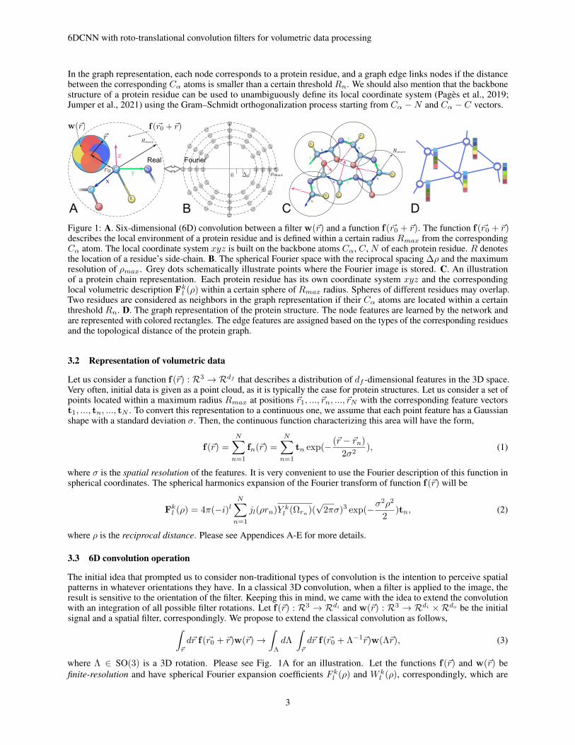
Here, we give a brief description of all steps of our method that are described in more detail below. Firstly, for eachresidue in the input protein molecule, we construct a function f(~r) that describes its local environment. More technically,this function is a set of 3D Gaussian-shaped features centered on the location of atoms within a certain distance Rmaxfrom the Cα atom of the corresponding residue (see Fig. 1A).

Then, for each function f(~r), we compute its spherical Fourier expansion coefficients Fkl (ρ). The angular resolution ofthe expansion is determined by the maximum order of spherical harmonics L. The radial resolution of the expansioncorresponds to the maximum reciprocal distance ρmax and is inversely proportional to the resolution σ of the real-spaceGaussian features as ρmax = π/σ (see Fig. 1B). Similarly, the radial spacing between the reciprocal points is inverselyproportional to the linear size of the data, ∆ρ = π/(2Rmax). Without loss of generality, we can set the number ofreciprocal radial points to be equal L, such that ρmax/∆ρ = L+ 1 = 2Rmax/σ.

Spherical Fourier coefficients Fkl (ρ) constitute the input for our network, along with the information about the transitionfrom the coordinate system of one residue to another. We start the network with the embedding block that reduces thedimensionality of the feature space. Then, we apply a series of 6D convolution blocks that consist of 6D convolution,normalization, and activation layers, followed by a message-passing layer. After a series of operations on continuousdata, we switch to the discrete representation and continue the network with graph convolutional layers (see Fig. 1C-D).

2


In the graph representation, each node corresponds to a protein residue, and a graph edge links nodes if the distancebetween the corresponding Cα atoms is smaller than a certain threshold Rn. We should also mention that the backbonestructure of a protein residue can be used to unambiguously define its local coordinate system (Pagès et al., 2019;Jumper et al., 2021) using the Gram–Schmidt orthogonalization process starting from Cα −N and Cα − C vectors.

<latexit sha1_base64="7VU86JVyhAUqfqZisyajkxfj/DI=">AAACDnicbVDLTgIxFO34RHyhLt00EhNXZAaNuiRx4xITeUSYkE65QEOnM2nvkJAJ/+DCrX6GO+PWX/Ar/AULzELAk7Q5Oefe3tsTxFIYdN1vZ219Y3NrO7eT393bPzgsHB3XTZRoDjUeyUg3A2ZACgU1FCihGWtgYSChEQzvpn5jBNqISD3iOAY/ZH0leoIztNITbY+Ap7rjTjqFoltyZ6CrxMtIkWSodgo/7W7EkxAUcsmMaXlujH7KNAouYZJvJwZixoesDy1LFQvB+Ols4wk9t0qX9iJtj0I6U/92pCw0ZhwGtjJkODDL3lT8z2sl2Lv1U6HiBEHx+aBeIilGdPp92hUaOMqxJYxrYXelfMA042hDWpgCRii0D9gb+ppJYxPylvNYJfVyybsuXT5cFSvlLKscOSVn5IJ45IZUyD2pkhrhRJEX8krenGfn3flwPuela07Wc0IW4Hz9AjPenNU=</latexit>

~r0

<latexit sha1_base64="CVW9z67XdOCHkpI44n6hzT0LCEk=">AAACDHicbVDLTgIxFL2DL8QX6tJNIzFxRWbQqEsSNy4xkUcCE9IpF2jodCZth4RM+AUXbvUz3Bm3/oNf4S9YYBYCnqTNyTn39t6eIBZcG9f9dnIbm1vbO/ndwt7+weFR8fikoaNEMayzSESqFVCNgkusG24EtmKFNAwENoPR/cxvjlFpHsknM4nRD+lA8j5n1FipRTpjZKmadoslt+zOQdaJl5ESZKh1iz+dXsSSEKVhgmrd9tzY+ClVhjOB00In0RhTNqIDbFsqaYjaT+f7TsmFVXqkHyl7pCFz9W9HSkOtJ2FgK0NqhnrVm4n/ee3E9O/8lMs4MSjZYlA/EcREZPZ50uMKmRETSyhT3O5K2JAqyoyNaGkKai6NfcDeOFBUaJuQt5rHOmlUyt5N+erxulStZFnl4QzO4RI8uIUqPEAN6sBAwAu8wpvz7Lw7H87nojTnZD2nsATn6xf6dZwy</latexit>

~r

z

xy

C

O

Cα

R

N<latexit sha1_base64="iBGB7b9cvkorwH+HK+StcPMPSGQ=">AAACDnicbVDLTgIxFO34RHyhLt00EhNXZAaNuiRx4xITeUSYkE65QEMfk7ZjJBP+wYVb/Qx3xq2/4Ff4CxaYhYAnaXNyzr29tyeKOTPW97+9ldW19Y3N3FZ+e2d3b79wcFg3KtEUalRxpZsRMcCZhJpllkMz1kBExKERDW8mfuMRtGFK3ttRDKEgfcl6jBLrpIe2HqhOKsjTuFMo+iV/CrxMgowUUYZqp/DT7iqaCJCWcmJMK/BjG6ZEW0Y5jPPtxEBM6JD0oeWoJAJMmE43HuNTp3RxT2l3pMVT9W9HSoQxIxG5SkHswCx6E/E/r5XY3nWYMhknFiSdDeolHFuFJ9/HXaaBWj5yhFDN3K6YDogm1LqQ5qaAYdK6B9wNfU24cQkFi3ksk3q5FFyWzu8uipVyllUOHaMTdIYCdIUq6BZVUQ1RJNELekVv3rP37n14n7PSFS/rOUJz8L5+AR+rnWQ=</latexit>max

<latexit sha1_base64="bQYRX303/hcUdQ9XDm7zpjUjqP4=">AAACD3icbVDLTgIxFO3gC/GFunTTSExckRk06pJEFy4xkUcChHTKBRo67aS9Y0IIH+HCrX6GO+PWT/Ar/AULzELAk7Q5Oefe3tsTxlJY9P1vL7O2vrG5ld3O7ezu7R/kD49qVieGQ5VrqU0jZBakUFBFgRIasQEWhRLq4fB26tefwFih1SOOYmhHrK9ET3CGTmq27kAioy0z0J18wS/6M9BVEqSkQFJUOvmfVlfzJAKFXDJrm4EfY3vMDAouYZJrJRZixoesD01HFYvAtsezlSf0zCld2tPGHYV0pv7tGLPI2lEUusqI4cAue1PxP6+ZYO+mPRYqThAUnw/qJZKiptP/064wwFGOHGHcCLcr5QNmGEeX0sIUsEKhe8Dd0DdMWpdQsJzHKqmVisFV8eLhslAupVllyQk5JeckINekTO5JhVQJJ5q8kFfy5j17796H9zkvzXhpzzFZgPf1C+wnnTc=</latexit>

<latexit sha1_base64="YWjRi2+zhDsbXwQW9g6uYjiXJFo=">AAACBXicbVDLTgIxFL2DL8QX6tJNIzFxRWbQqEsSNy4hkUcCE9IpF2jodCZtx4RMWLtwq5/hzrj1O/wKf8ECsxDwJG1Ozrm39/YEseDauO63k9vY3Nreye8W9vYPDo+KxydNHSWKYYNFIlLtgGoUXGLDcCOwHSukYSCwFYzvZ37rCZXmkXw0kxj9kA4lH3BGjZXqbq9YcsvuHGSdeBkpQYZar/jT7UcsCVEaJqjWHc+NjZ9SZTgTOC10E40xZWM6xI6lkoao/XS+6JRcWKVPBpGyRxoyV/92pDTUehIGtjKkZqRXvZn4n9dJzODOT7mME4OSLQYNEkFMRGa/Jn2ukBkxsYQyxe2uhI2ooszYbJamoObS2AfsjUNFhbYJeat5rJNmpezdlK/q16VqJcsqD2dwDpfgwS1U4QFq0AAGCC/wCm/Os/PufDifi9Kck/WcwhKcr18eCpj4</latexit>

0

Real Fourier

<latexit sha1_base64="3BdVab5okB/Kn0CtYAemrJZqKOE=">AAACC3icbVDLTgIxFL3jE/GFunTTSExckRk16pLoxiUaeSQwIZ1ygYZOZ9J2jGTCJ7hwq5/hzrj1I/wKf8ECsxDwJG1Ozrm39/YEseDauO63s7S8srq2ntvIb25t7+wW9vZrOkoUwyqLRKQaAdUouMSq4UZgI1ZIw0BgPRjcjP36IyrNI/lghjH6Ie1J3uWMGivV79tpSJ9G7ULRLbkTkEXiZaQIGSrtwk+rE7EkRGmYoFo3PTc2fkqV4UzgKN9KNMaUDWgPm5ZKGqL208m6I3JslQ7pRsoeachE/duR0lDrYRjYypCavp73xuJ/XjMx3Ss/5TJODEo2HdRNBDERGf+ddLhCZsTQEsoUt7sS1qeKMmMTmpmCmktjH7A39hQV2ibkzeexSGqnJe+idHZ3XixfZ1nl4BCO4AQ8uIQy3EIFqsBgAC/wCm/Os/PufDif09IlJ+s5gBk4X7+CnJwD</latexit>

Rmax

<latexit sha1_base64="FoU1OMfHsrpXKzUw479dKMM52t8=">AAACJnicbVDLSgMxFM3UV62vqks3wSJUhDKjoi6LblxWsA/olJJJ77ShmcyQZAplmK3f4sKtfoY7EXf+gb9g2s7Cth5IOJxzb+7N8SLOlLbtLyu3srq2vpHfLGxt7+zuFfcPGiqMJYU6DXkoWx5RwJmAumaaQyuSQAKPQ9Mb3k385gikYqF41OMIOgHpC+YzSrSRukWM3YDogecnflp2R0AT2bVTfIZnPD3tFkt2xZ4CLxMnIyWUodYt/ri9kMYBCE05Uart2JHuJERqRjmkBTdWEBE6JH1oGypIAKqTTH+S4hOj9LAfSnOExlP1b0dCAqXGgWcqJ2urRW8i/ue1Y+3fdBImoliDoLNBfsyxDvEkFtxjEqjmY0MIlczsiumASEK1CW9uCigmtHnA3NCXhCuTkLOYxzJpnFecq8rFw2WpeptllUdH6BiVkYOuURXdoxqqI4qe0At6RW/Ws/VufVifs9KclfUcojlY3792IKXe</latexit>

f(~r0 + ~r)<latexit sha1_base64="B6lpXtieKszQpTA7oMCCLfdj438=">AAACGnicbVDLTgIxFO3gC/E1PnZuGokJbsiMGnVJdOMSE0EShpBOuQMNnc6k7WBwwp+4cKuf4c64deNX+At2gIWAJ2lzcs595fgxZ0o7zreVW1peWV3Lrxc2Nre2d+zdvbqKEkmhRiMeyYZPFHAmoKaZ5tCIJZDQ5/Dg928y/2EAUrFI3OthDK2QdAULGCXaSG37wAuJ7vlB+jgqeQOgqRyd4LZddMrOGHiRuFNSRFNU2/aP14loEoLQlBOlmq4T61ZKpGaUw6jgJQpiQvukC01DBQlBtdLx9SN8bJQODiJpntB4rP7tSEmo1DD0TWV2q5r3MvE/r5no4KqVMhEnGgSdLAoSjnWEsyhwh0mgmg8NIVQycyumPSIJ1SawmS2gmNBmgPmhKwlXJiF3Po9FUj8tuxfls7vzYuV6mlUeHaIjVEIuukQVdIuqqIYoekIv6BW9Wc/Wu/VhfU5Kc9a0Zx/NwPr6BeeBoXk=</latexit>

w(~r)

N

Cα R

NC

O

Cα

R

N

C

O

Cα R

N

C

O

Cα

R

C

OCα

R

x

yzz

zz

z

x

x

x x

y

y

yy

<latexit sha1_base64="3BdVab5okB/Kn0CtYAemrJZqKOE=">AAACC3icbVDLTgIxFL3jE/GFunTTSExckRk16pLoxiUaeSQwIZ1ygYZOZ9J2jGTCJ7hwq5/hzrj1I/wKf8ECsxDwJG1Ozrm39/YEseDauO63s7S8srq2ntvIb25t7+wW9vZrOkoUwyqLRKQaAdUouMSq4UZgI1ZIw0BgPRjcjP36IyrNI/lghjH6Ie1J3uWMGivV79tpSJ9G7ULRLbkTkEXiZaQIGSrtwk+rE7EkRGmYoFo3PTc2fkqV4UzgKN9KNMaUDWgPm5ZKGqL208m6I3JslQ7pRsoeachE/duR0lDrYRjYypCavp73xuJ/XjMx3Ss/5TJODEo2HdRNBDERGf+ddLhCZsTQEsoUt7sS1qeKMmMTmpmCmktjH7A39hQV2ibkzeexSGqnJe+idHZ3XixfZ1nl4BCO4AQ8uIQy3EIFqsBgAC/wCm/Os/PufDif09IlJ+s5gBk4X7+CnJwD</latexit>

Rmax

A B C DFigure 1: A. Six-dimensional (6D) convolution between a filter w(~r) and a function f(~r0 + ~r). The function f(~r0 + ~r)describes the local environment of a protein residue and is defined within a certain radius Rmax from the correspondingCα atom. The local coordinate system xyz is built on the backbone atoms Cα, C, N of each protein residue. R denotesthe location of a residue’s side-chain. B. The spherical Fourier space with the reciprocal spacing ∆ρ and the maximumresolution of ρmax. Grey dots schematically illustrate points where the Fourier image is stored. C. An illustrationof a protein chain representation. Each protein residue has its own coordinate system xyz and the correspondinglocal volumetric description Fkl (ρ) within a certain sphere of Rmax radius. Spheres of different residues may overlap.Two residues are considered as neighbors in the graph representation if their Cα atoms are located within a certainthreshold Rn. D. The graph representation of the protein structure. The node features are learned by the network andare represented with colored rectangles. The edge features are assigned based on the types of the corresponding residuesand the topological distance of the protein graph.

3.2 Representation of volumetric data

Let us consider a function f(~r) : R3 → Rdf that describes a distribution of df -dimensional features in the 3D space.Very often, initial data is given as a point cloud, as it is typically the case for protein structures. Let us consider a set ofpoints located within a maximum radius Rmax at positions ~r1, ..., ~rn, ..., ~rN with the corresponding feature vectorst1, ..., tn, ..., tN . To convert this representation to a continuous one, we assume that each point feature has a Gaussianshape with a standard deviation σ. Then, the continuous function characterizing this area will have the form,

f(~r) =

N∑n=1

fn(~r) =

N∑n=1

tn exp(− (~r − ~rn)

2σ2), (1)

where σ is the spatial resolution of the features. It is very convenient to use the Fourier description of this function inspherical coordinates. The spherical harmonics expansion of the Fourier transform of function f(~r) will be

Fkl (ρ) = 4π(−i)lN∑n=1

jl(ρrn)Y kl (Ωrn)(√

2πσ)3 exp(−σ2ρ2

2)tn, (2)

where ρ is the reciprocal distance. Please see Appendices A-E for more details.

3.3 6D convolution operation

The initial idea that prompted us to consider non-traditional types of convolution is the intention to perceive spatialpatterns in whatever orientations they have. In a classical 3D convolution, when a filter is applied to the image, theresult is sensitive to the orientation of the filter. Keeping this in mind, we came with the idea to extend the convolutionwith an integration of all possible filter rotations. Let f(~r) : R3 → Rdi and w(~r) : R3 → Rdi ×Rdo be the initialsignal and a spatial filter, correspondingly. We propose to extend the classical convolution as follows,∫

~r

d~r f(~r0 + ~r)w(~r)→∫

Λ

dΛ

∫~r

d~r f(~r0 + Λ−1~r)w(Λ~r), (3)

where Λ ∈ SO(3) is a 3D rotation. Please see Fig. 1A for an illustration. Let the functions f(~r) and w(~r) befinite-resolution and have spherical Fourier expansion coefficients F kl (ρ) and W k

l (ρ), correspondingly, which are

3


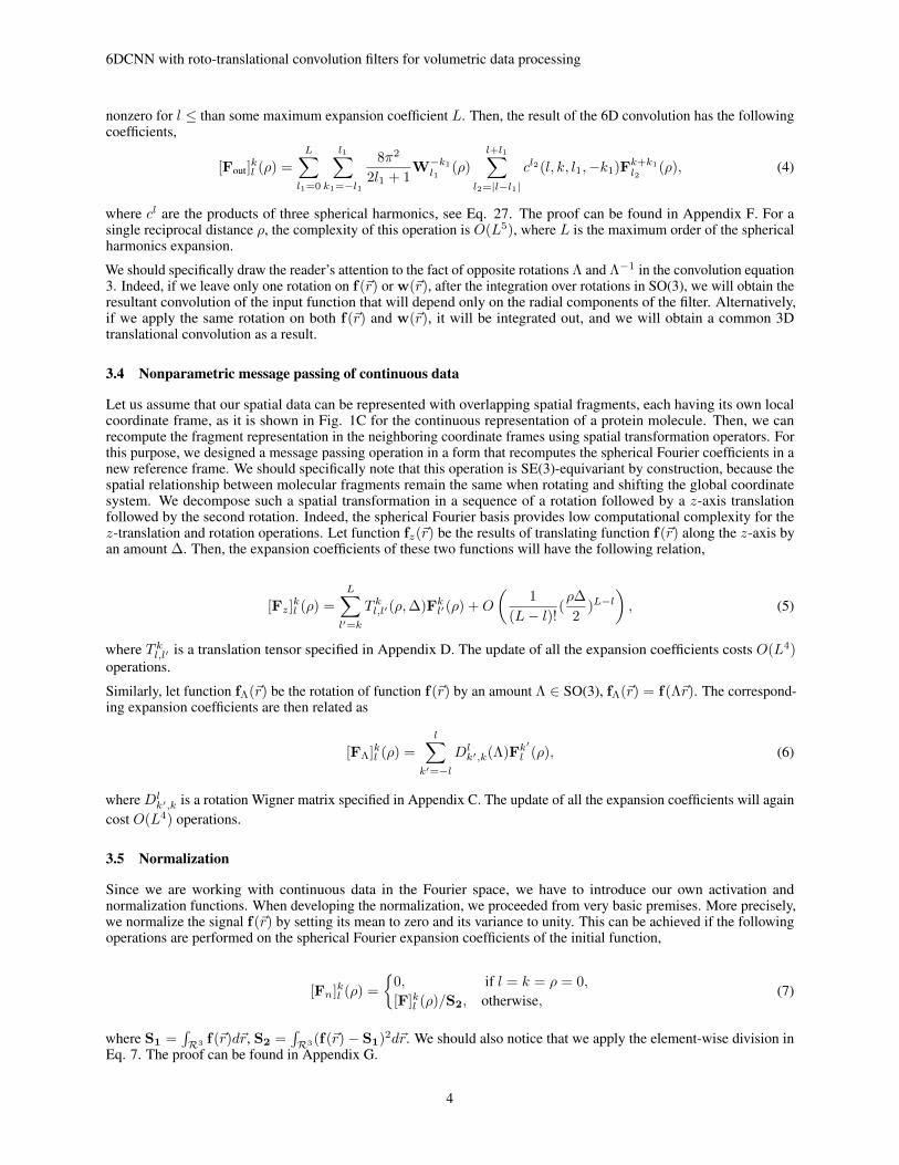
nonzero for l ≤ than some maximum expansion coefficient L. Then, the result of the 6D convolution has the followingcoefficients,

[Fout]kl (ρ) =

L∑l1=0

l1∑k1=−l1

8π2

2l1 + 1W−k1

l1(ρ)

l+l1∑l2=|l−l1|

cl2(l, k, l1,−k1)Fk+k1l2

(ρ), (4)

where cl are the products of three spherical harmonics, see Eq. 27. The proof can be found in Appendix F. For asingle reciprocal distance ρ, the complexity of this operation is O(L5), where L is the maximum order of the sphericalharmonics expansion.

We should specifically draw the reader’s attention to the fact of opposite rotations Λ and Λ−1 in the convolution equation3. Indeed, if we leave only one rotation on f(~r) or w(~r), after the integration over rotations in SO(3), we will obtain theresultant convolution of the input function that will depend only on the radial components of the filter. Alternatively,if we apply the same rotation on both f(~r) and w(~r), it will be integrated out, and we will obtain a common 3Dtranslational convolution as a result.

3.4 Nonparametric message passing of continuous data

Let us assume that our spatial data can be represented with overlapping spatial fragments, each having its own localcoordinate frame, as it is shown in Fig. 1C for the continuous representation of a protein molecule. Then, we canrecompute the fragment representation in the neighboring coordinate frames using spatial transformation operators. Forthis purpose, we designed a message passing operation in a form that recomputes the spherical Fourier coefficients in anew reference frame. We should specifically note that this operation is SE(3)-equivariant by construction, because thespatial relationship between molecular fragments remain the same when rotating and shifting the global coordinatesystem. We decompose such a spatial transformation in a sequence of a rotation followed by a z-axis translationfollowed by the second rotation. Indeed, the spherical Fourier basis provides low computational complexity for thez-translation and rotation operations. Let function fz(~r) be the results of translating function f(~r) along the z-axis byan amount ∆. Then, the expansion coefficients of these two functions will have the following relation,

[Fz]kl (ρ) =

L∑l′=k

T kl,l′(ρ,∆)Fkl′(ρ) +O

(1

(L− l)!(ρ∆

2)L−l

), (5)

where T kl,l′ is a translation tensor specified in Appendix D. The update of all the expansion coefficients costs O(L4)operations.

Similarly, let function fΛ(~r) be the rotation of function f(~r) by an amount Λ ∈ SO(3), fΛ(~r) = f(Λ~r). The correspond-ing expansion coefficients are then related as

[FΛ]kl (ρ) =

l∑k′=−l

Dlk′,k(Λ)Fk

′

l (ρ), (6)

where Dlk′,k is a rotation Wigner matrix specified in Appendix C. The update of all the expansion coefficients will again

cost O(L4) operations.

3.5 Normalization

Since we are working with continuous data in the Fourier space, we have to introduce our own activation andnormalization functions. When developing the normalization, we proceeded from very basic premises. More precisely,we normalize the signal f(~r) by setting its mean to zero and its variance to unity. This can be achieved if the followingoperations are performed on the spherical Fourier expansion coefficients of the initial function,

[Fn]kl (ρ) =

0, if l = k = ρ = 0,

[F]kl (ρ)/S2, otherwise,(7)

where S1 =∫R3 f(~r)d~r, S2 =

∫R3(f(~r)− S1)2d~r. We should also notice that we apply the element-wise division in

Eq. 7. The proof can be found in Appendix G.

4


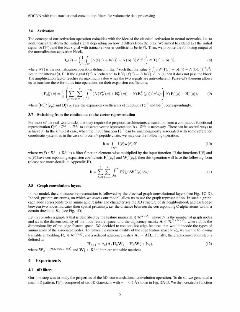
3.6 Activation

The concept of our activation operation coincides with the idea of the classical activation in neural networks, i.e. tononlinearly transform the initial signal depending on how it differs from the bias. We aimed to extend Let the initialsignal be f(~r), and the bias signal with trainable Fourier coefficients be b(~r). Then, we propose the following output ofthe normalization-activation block,

fa(~r) =

(1

4

∫R3

(N(f(~r) + b(~r))−N(b(~r)))2d3~r

)N(f(~r) + b(~r)), (8)

where N() is the normalization operation defined in Eq. 7 such that the value 14

∫R3(N(f(~r) + b(~r))−N(b(~r)))2d3~r

lies in the interval [0, 1]. If the signal f(~r) is ’coherent’ to b(~r) , f(~r) = Kb(~r),K > 0, then it does not pass the block.The amplification factor reaches its maximum value when the two signals are anti-coherent. Parseval’s theorem allowsus to translate these formulas into operations on their expansion coefficients,

[Fa]kl (ρ) =1

4

L∑l′=0

l′∑k′=−l′

∫ ∞0

(N(Fk′

l′ (ρ) + Bk′

l′ (ρ))−N(Bk′

l′ (ρ)))2ρ2dρ

N(Fkl (ρ) + Bkl (ρ)), (9)

where [Fa]kl (ρp) and Bkl (ρp) are the expansion coefficients of functions f(~r) and b(~r), correspondingly.

3.7 Switching from the continuous to the vector representation

For most of the real-world tasks that may require the proposed architecture, a transition from a continuous functionalrepresentation f(~r) : R3 → Rdf to a discrete vector representation h ∈ Rdf is necessary. There can be several ways toachieve it. In the simplest case, when the input function f(~r) can be unambiguously associated with some referencecoordinate system, as in the case of protein’s peptide chain, we may use the following operation,

h =

∫R3

f(~r)w(~r)d~r, (10)

where w(~r) : R3 → Rdf is a filter function element-wise multiplied by the input function. If the functions f(~r) andw(~r) have corresponding expansion coefficients Fkl (ρp) and Wk

l (ρp), then this operation will have the following form(please see more details in Appendix H),

h =

L∑l=0

l∑k=−l

∫ ∞0

Fkl (ρ)Wk

l (ρ)ρ2dρ. (11)

3.8 Graph convolutions layers

In our model, the continuous representation is followed by the classical graph convolutional layers (see Fig. 1C-D).Indeed, protein structures, on which we assess our model, allow us to use the graph representation. In such a graph,each node corresponds to an amino acid residue and characterizes the 3D structure of its neighborhood, and each edgebetween two nodes indicates their spatial proximity, i.e. the distance between the corresponding C-alpha atoms within acertain threshold Rn (see Fig. 1D).

Let us consider a graph G that is described by the feature matrix H ∈ RN×dv , where N is the number of graph nodesand dv is the dimensionality of the node feature space, and the adjacency matrix A ∈ RN×N×de , where de is thedimensionality of the edge feature space. We decided to use one-hot edge features that would encode the types ofamino acids of the associated nodes. To reduce the dimensionality of the edge feature space to d′e, we use the followingtrainable embedding Re ∈ Rde×d

′e , and a reduced adjacency matrix Ar = ARe. Finally, the graph convolution step is

defined asHk+1 = σa(ArHkWk + HkW

sk + bk), (12)

where Wk ∈ Rdk×dk+1×d′e and Wsk ∈ Rdk×dk+1 are trainable matrices.

4 Experiments

4.1 6D filters

Our first step was to study the properties of the 6D roto-translational convolution operation. To do so, we generated asmall 3D pattern, f(~r), composed of six 3D Gaussians with σ = 0.4 Å shown in Fig. 2A-B. We then created a function

5


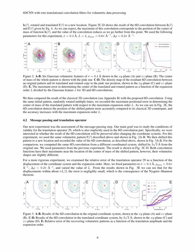
h(~r), rotated and translated f(~r) to a new location. Figure 2C-D shows the result of the 6D convolution between h(~r)and f(~r) given by Eq. 4. As we can expect, the maximum of this convolution corresponds to the position of the center ofmass of function h(~r), and the value of the convolution reduces as we go further from this point. We used the followingparameters for this experiment, σ = 0.4 Å, L = 4, ρmax = 0.6π Å−1, ∆ρ = 0.2π Å−1.

2.0

1.5

1.0

0.5

0.0

0.5

1.0

1.5

2.0

2.0

1.5

1.0

0.5

0.0

0.5

1.0

1.5

2.0

2 1 0 1 2X axis

Yax

is

0.2000.400

0.800

0.20

0

0.800

0.20

00.400

0.800

0.400

2 1 0 1 2X axis

Zax

is

0.200

0.400

0.800

0.400

0.400

0.800

Yax

is

Zax

is

A B

2 4 6 8 10 12Expansion order

10-1

100

Max

imum

erro

r

3D convolution6D convolution

E

4 2 0 2 4X axis

4

2

0

2

4

0.000

0.000

0.080

0.16

0

0.240

0.32

0

C

4 2 0 2 4X axis

4

2

0

2

4

0.000

0.000

0.080

0.16

0

0.2400

.320

D

Figure 2: A-B. Six Gaussian volumetric features of σ = 0.4 Å shown in the xy-plane (A) and xz-plane (B). The centerof mass of the whole pattern is shown with the pink star. C-D. The density map of the resultant 6D convolution betweenan original pattern and its translated and rotated copy to the pink star position, shown in the xy-plane (C) and xz-plane(D). E. The maximum error in determining the center of the translated and rotated pattern as a function of the expansionorder L divided by the Gaussian feature σ for 3D and 6D convolutions.

We then compared the result of the classical 3D convolution (see Appendix B) with the proposed 6D convolution. Usingthe same initial pattern, randomly rotated multiple times, we recorded the maximum positional error in determining thecenter of mass of the translated pattern with respect to the maximum expansion order L. As we can see in Fig. 2E, the6D convolution detects the position of the shifted pattern more accurately compared to its classical 3D counterpart, andthe accuracy increases with the maximum expansion order L.

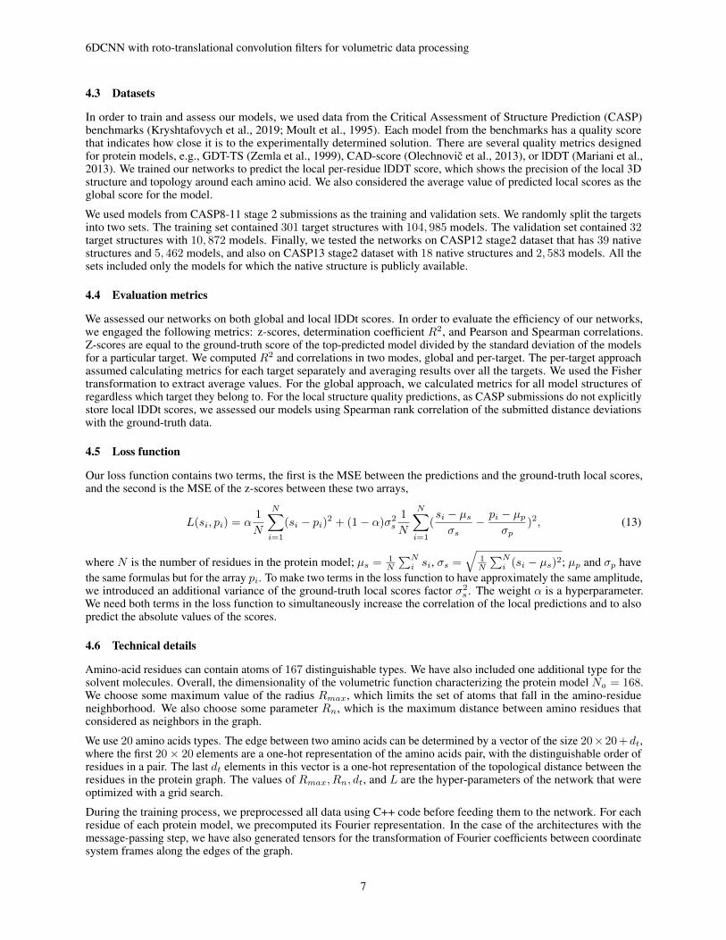
4.2 Message passing and translation operator

Our next experiment was the assessment of the message-passing step. Our main goal was to study the conditions ofvalidity for the translation operator 29, which is also implicitly used in the 6D convolution part. Specifically, we wereinterested in whether the result of the 6D convolution will be preserved after changing the coordinate systems. For thisexperiment, we used the same volumetric pattern f(~r) described above and shown in Fig. 2A-B. We then shifted thispattern to a new location and recorded the value of the 6D convolution, as described above, shown in Fig. 3A-B. For thecomparison, we computed the same 6D convolution from a different coordinated system, shifted by 3

√3 Å from the

original one. We used parameters from the previous experiment. The result is shown in Fig. 3C-D. Both convolutionfunctions have their maximums near the location of the center of mass of the shifted pattern, however, their volumetricshapes are slightly different.

For a more rigorous experiment, we examined the relative error of the translation operator 29 as a function of thedisplacement of the coordinate system and the expansion order. Here, we fixed parameters to σ = 0.4 Å, ρmax = 0.6πÅ−1, ∆ρ = 0.2π Å−1, and varied the value of L. From the results shown in Fig. 3E we can see that for thedisplacements within about σL/2, the error is negligibly small, which is the consequence of the Nyquist–Shannontheorem.

Yaxis

Zaxis

E

4 2 0 2 4X axis

4

2

0

2

4

0.000

0.000

0.080

0.160

0.240

0.320

A

4 2 0 2 4X axis

4

2

0

2

4

0.000

0.000

0.080

0.160

0.2400

.320

B

4 2 0 2 4X axis

4

2

0

2

4

Yaxis

0.000

0.000

0.080

0.160

0.240

0.320

X axis4 2 0 2 4

4

2

0

2

4

0.000

0.000

0.080

0.160

0.2400.3

20

Zaxis

C D

0 5 10 15

0.0

0.2

0.4

0.6

0.8

Relative

error

L = 5

L = 10

L = 15

L = 25

Displacement, Å

Figure 3: A-B. Results of the 6D convolution in the original coordinate system, shown in the xy-plane (A) and xz-plane(B). C-D. Results of the 6D convolution in the translated coordinate system, by 3

√3 Å, shown in the xy-plane (C) and

xz-plane (D). E. Relative error of the recovering volumetric patterns as a function of the translation amplitude and theexpansion order.

6


4.3 Datasets

In order to train and assess our models, we used data from the Critical Assessment of Structure Prediction (CASP)benchmarks (Kryshtafovych et al., 2019; Moult et al., 1995). Each model from the benchmarks has a quality scorethat indicates how close it is to the experimentally determined solution. There are several quality metrics designedfor protein models, e.g., GDT-TS (Zemla et al., 1999), CAD-score (Olechnovic et al., 2013), or lDDT (Mariani et al.,2013). We trained our networks to predict the local per-residue lDDT score, which shows the precision of the local 3Dstructure and topology around each amino acid. We also considered the average value of predicted local scores as theglobal score for the model.

We used models from CASP8-11 stage 2 submissions as the training and validation sets. We randomly split the targetsinto two sets. The training set contained 301 target structures with 104, 985 models. The validation set contained 32target structures with 10, 872 models. Finally, we tested the networks on CASP12 stage2 dataset that has 39 nativestructures and 5, 462 models, and also on CASP13 stage2 dataset with 18 native structures and 2, 583 models. All thesets included only the models for which the native structure is publicly available.

4.4 Evaluation metrics

We assessed our networks on both global and local lDDt scores. In order to evaluate the efficiency of our networks,we engaged the following metrics: z-scores, determination coefficient R2, and Pearson and Spearman correlations.Z-scores are equal to the ground-truth score of the top-predicted model divided by the standard deviation of the modelsfor a particular target. We computed R2 and correlations in two modes, global and per-target. The per-target approachassumed calculating metrics for each target separately and averaging results over all the targets. We used the Fishertransformation to extract average values. For the global approach, we calculated metrics for all model structures ofregardless which target they belong to. For the local structure quality predictions, as CASP submissions do not explicitlystore local lDDt scores, we assessed our models using Spearman rank correlation of the submitted distance deviationswith the ground-truth data.

4.5 Loss function

Our loss function contains two terms, the first is the MSE between the predictions and the ground-truth local scores,and the second is the MSE of the z-scores between these two arrays,

L(si, pi) = α1

N

N∑i=1

(si − pi)2 + (1− α)σ2s

1

N

N∑i=1

(si − µsσs

− pi − µpσp

)2, (13)

where N is the number of residues in the protein model; µs = 1N

∑Ni si, σs =

√1N

∑Ni (si − µs)2; µp and σp have

the same formulas but for the array pi. To make two terms in the loss function to have approximately the same amplitude,we introduced an additional variance of the ground-truth local scores factor σ2

s . The weight α is a hyperparameter.We need both terms in the loss function to simultaneously increase the correlation of the local predictions and to alsopredict the absolute values of the scores.

4.6 Technical details

Amino-acid residues can contain atoms of 167 distinguishable types. We have also included one additional type for thesolvent molecules. Overall, the dimensionality of the volumetric function characterizing the protein model Na = 168.We choose some maximum value of the radius Rmax, which limits the set of atoms that fall in the amino-residueneighborhood. We also choose some parameter Rn, which is the maximum distance between amino residues thatconsidered as neighbors in the graph.

We use 20 amino acids types. The edge between two amino acids can be determined by a vector of the size 20×20 +dt,where the first 20× 20 elements are a one-hot representation of the amino acids pair, with the distinguishable order ofresidues in a pair. The last dt elements in this vector is a one-hot representation of the topological distance between theresidues in the protein graph. The values of Rmax, Rn, dt, and L are the hyper-parameters of the network that wereoptimized with a grid search.

During the training process, we preprocessed all data using C++ code before feeding them to the network. For eachresidue of each protein model, we precomputed its Fourier representation. In the case of the architectures with themessage-passing step, we have also generated tensors for the transformation of Fourier coefficients between coordinatesystem frames along the edges of the graph.

7


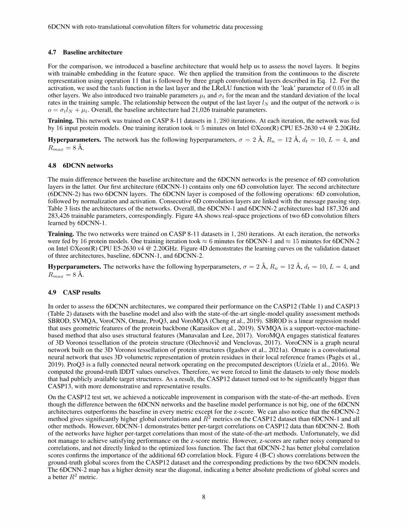
4.7 Baseline architecture

For the comparison, we introduced a baseline architecture that would help us to assess the novel layers. It beginswith trainable embedding in the feature space. We then applied the transition from the continuous to the discreterepresentation using operation 11 that is followed by three graph convolutional layers described in Eq. 12. For theactivation, we used the tanh function in the last layer and the LReLU function with the ’leak’ parameter of 0.05 in allother layers. We also introduced two trainable parameters µt and σt for the mean and the standard deviation of the localrates in the training sample. The relationship between the output of the last layer lN and the output of the network o iso = σtlN + µt. Overall, the baseline architecture had 21,026 trainable parameters.

Training. This network was trained on CASP 8-11 datasets in 1, 280 iterations. At each iteration, the network was fedby 16 input protein models. One training iteration took ≈ 5 minutes on Intel ©Xeon(R) CPU E5-2630 v4 @ 2.20GHz.

Hyperparameters. The network has the following hyperparameters, σ = 2 Å, Rn = 12 Å, dt = 10, L = 4, andRmax = 8 Å.

4.8 6DCNN networks

The main difference between the baseline architecture and the 6DCNN networks is the presence of 6D convolutionlayers in the latter. Our first architecture (6DCNN-1) contains only one 6D convolution layer. The second architecture(6DCNN-2) has two 6DCNN layers. The 6DCNN layer is composed of the following operations: 6D convolution,followed by normalization and activation. Consecutive 6D convolution layers are linked with the message passing step.Table 3 lists the architectures of the networks. Overall, the 6DCNN-1 and 6DCNN-2 architectures had 187,326 and283,426 trainable parameters, correspondingly. Figure 4A shows real-space projections of two 6D convolution filterslearned by 6DCNN-1.

Training. The two networks were trained on CASP 8-11 datasets in 1, 280 iterations. At each iteration, the networkswere fed by 16 protein models. One training iteration took ≈ 6 minutes for 6DCNN-1 and ≈ 15 minutes for 6DCNN-2on Intel ©Xeon(R) CPU E5-2630 v4 @ 2.20GHz. Figure 4D demonstrates the learning curves on the validation datasetof three architectures, baseline, 6DCNN-1, and 6DCNN-2.

Hyperparameters. The networks have the following hyperparameters, σ = 2 Å, Rn = 12 Å, dt = 10, L = 4, andRmax = 8 Å.

4.9 CASP results

In order to assess the 6DCNN architectures, we compared their performance on the CASP12 (Table 1) and CASP13(Table 2) datasets with the baseline model and also with the state-of-the-art single-model quality assessment methodsSBROD, SVMQA, VoroCNN, Ornate, ProQ3, and VoroMQA (Cheng et al., 2019). SBROD is a linear regression modelthat uses geometric features of the protein backbone (Karasikov et al., 2019). SVMQA is a support-vector-machine-based method that also uses structural features (Manavalan and Lee, 2017). VoroMQA engages statistical featuresof 3D Voronoi tessellation of the protein structure (Olechnovic and Venclovas, 2017). VoroCNN is a graph neuralnetwork built on the 3D Voronoi tessellation of protein structures (Igashov et al., 2021a). Ornate is a convolutionalneural network that uses 3D volumetric representation of protein residues in their local reference frames (Pagès et al.,2019). ProQ3 is a fully connected neural network operating on the precomputed descriptors (Uziela et al., 2016). Wecomputed the ground-truth lDDT values ourselves. Therefore, we were forced to limit the datasets to only those modelsthat had publicly available target structures. As a result, the CASP12 dataset turned out to be significantly bigger thanCASP13, with more demonstrative and representative results.

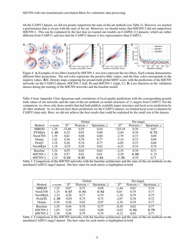
On the CASP12 test set, we achieved a noticeable improvement in comparison with the state-of-the-art methods. Eventhough the difference between the 6DCNN networks and the baseline model performance is not big, one of the 6DCNNarchitectures outperforms the baseline in every metric except for the z-score. We can also notice that the 6DCNN-2method gives significantly higher global correlations and R2 metrics on the CASP12 dataset than 6DCNN-1 and allother methods. However, 6DCNN-1 demonstrates better per-target correlations on CASP12 data than 6DCNN-2. Bothof the networks have higher per-target correlations than most of the state-of-the-art methods. Unfortunately, we didnot manage to achieve satisfying performance on the z-score metric. However, z-scores are rather noisy compared tocorrelations, and not directly linked to the optimized loss function. The fact that 6DCNN-2 has better global correlationscores confirms the importance of the additional 6D correlation block. Figure 4 (B-C) shows correlations between theground-truth global scores from the CASP12 dataset and the corresponding predictions by the two 6DCNN models.The 6DCNN-2 map has a higher density near the diagonal, indicating a better absolute predictions of global scores anda better R2 metric.

8


On the CASP13 dataset, we did not greatly outperform the state-of-the-art methods (see Table 2). However, we reacheda performance that is on par with the state of the art. Moreover, we should notice that 6DCNN-2 did not outperform6DCNN-1. This can be explained by the fact that we trained our models on CASP[8-11] datasets, which are ratherdifferent from CASP13, and also that the CASP13 dataset is less representative than CASP12.

<latexit sha1_base64="8D4QOd2n8PgERh3VUTqHeZ37gLI=">AAACBXicbVC7TsMwFL0pr1JeBUaWiAqJqUoAAWMlFsZWog+pDZXj3rRWHSeyHaQo6szACp/Bhlj5Dr6CX8BtM9CWI9k6Oude3+vjx5wp7TjfVmFtfWNzq7hd2tnd2z8oHx61VJRIik0a8Uh2fKKQM4FNzTTHTiyRhD7Htj++m/rtJ5SKReJBpzF6IRkKFjBKtJEaab9ccarODPYqcXNSgRz1fvmnN4hoEqLQlBOluq4Tay8jUjPKcVLqJQpjQsdkiF1DBQlRedls0Yl9ZpSBHUTSHKHtmfq3IyOhUmnom8qQ6JFa9qbif1430cGtlzERJxoFnQ8KEm7ryJ7+2h4wiVTz1BBCJTO72nREJKHaZLMwBRUT2jxgbhxKwpVJyF3OY5W0LqrudfWycVWpPeZZFeEETuEcXLiBGtxDHZpAAeEFXuHNerberQ/rc15asPKeY1iA9fULoi+ZbQ==</latexit>y

0.0 0.2 0.4 0.6 0.8 1.0

Ground-truth lDDT score0.0

0.2

0.4

0.6

0.8

1.0

PredictedlDDTscore

2.5

5.0

7.5

10.0

12.5

15.0

17.5

20.0

2.5

5.0

7.5

10.0

12.5

15.0

17.5

20.0

0.0 0.2 0.4 0.6 0.8 1.0

Ground-truth lDDT score0.0

0.2

0.4

0.6

0.8

1.0

PredictedlDDTscore

<latexit sha1_base64="5RJHMMKQ4G2VNlGJFDUZvjcNvPg=">AAACBXicbVDLTgIxFL2DL8QX6tJNIzFxRWbUqEsSNy4hkUcCI+mUO9DQ6UzajpEQ1i7c6me4M279Dr/CX7DALAQ9SZuTc+7tvT1BIrg2rvvl5FZW19Y38puFre2d3b3i/kFDx6liWGexiFUroBoFl1g33AhsJQppFAhsBsObqd98QKV5LO/MKEE/on3JQ86osVLtsVssuWV3BvKXeBkpQYZqt/jd6cUsjVAaJqjWbc9NjD+mynAmcFLopBoTyoa0j21LJY1Q++PZohNyYpUeCWNljzRkpv7uGNNI61EU2MqImoFe9qbif147NeG1P+YySQ1KNh8UpoKYmEx/TXpcITNiZAllittdCRtQRZmx2SxMQc2lsQ/YG/uKCm0T8pbz+EsaZ2XvsnxeuyhV7rOs8nAEx3AKHlxBBW6hCnVggPAML/DqPDlvzrvzMS/NOVnPISzA+fwBoI6ZbA==</latexit>x

<latexit sha1_base64="TBYTu25pkXPPT7+IwmLDkuXZwps=">AAACBXicbVDLTgIxFO3gC/GFunTTSExckRk16pLEjUtI5JHASDrlDjR0OpP2jgkS1i7c6me4M279Dr/CX7DALAQ9SZuTc+7tvT1BIoVB1/1yciura+sb+c3C1vbO7l5x/6Bh4lRzqPNYxroVMANSKKijQAmtRAOLAgnNYHgz9ZsPoI2I1R2OEvAj1lciFJyhlWqP3WLJLbsz0L/Ey0iJZKh2i9+dXszTCBRyyYxpe26C/phpFFzCpNBJDSSMD1kf2pYqFoHxx7NFJ/TEKj0axtoehXSm/u4Ys8iYURTYyojhwCx7U/E/r51ieO2PhUpSBMXng8JUUozp9Ne0JzRwlCNLGNfC7kr5gGnG0WazMAWMUGgfsDf0NZPGJuQt5/GXNM7K3mX5vHZRqtxnWeXJETkmp8QjV6RCbkmV1AknQJ7JC3l1npw35935mJfmnKznkCzA+fwBo9CZbg==</latexit>z<latexit sha1_base64="TBYTu25pkXPPT7+IwmLDkuXZwps=">AAACBXicbVDLTgIxFO3gC/GFunTTSExckRk16pLEjUtI5JHASDrlDjR0OpP2jgkS1i7c6me4M279Dr/CX7DALAQ9SZuTc+7tvT1BIoVB1/1yciura+sb+c3C1vbO7l5x/6Bh4lRzqPNYxroVMANSKKijQAmtRAOLAgnNYHgz9ZsPoI2I1R2OEvAj1lciFJyhlWqP3WLJLbsz0L/Ey0iJZKh2i9+dXszTCBRyyYxpe26C/phpFFzCpNBJDSSMD1kf2pYqFoHxx7NFJ/TEKj0axtoehXSm/u4Ys8iYURTYyojhwCx7U/E/r51ieO2PhUpSBMXng8JUUozp9Ne0JzRwlCNLGNfC7kr5gGnG0WazMAWMUGgfsDf0NZPGJuQt5/GXNM7K3mX5vHZRqtxnWeXJETkmp8QjV6RCbkmV1AknQJ7JC3l1npw35935mJfmnKznkCzA+fwBo9CZbg==</latexit>z

<latexit sha1_base64="TBYTu25pkXPPT7+IwmLDkuXZwps=">AAACBXicbVDLTgIxFO3gC/GFunTTSExckRk16pLEjUtI5JHASDrlDjR0OpP2jgkS1i7c6me4M279Dr/CX7DALAQ9SZuTc+7tvT1BIoVB1/1yciura+sb+c3C1vbO7l5x/6Bh4lRzqPNYxroVMANSKKijQAmtRAOLAgnNYHgz9ZsPoI2I1R2OEvAj1lciFJyhlWqP3WLJLbsz0L/Ey0iJZKh2i9+dXszTCBRyyYxpe26C/phpFFzCpNBJDSSMD1kf2pYqFoHxx7NFJ/TEKj0axtoehXSm/u4Ys8iYURTYyojhwCx7U/E/r51ieO2PhUpSBMXng8JUUozp9Ne0JzRwlCNLGNfC7kr5gGnG0WazMAWMUGgfsDf0NZPGJuQt5/GXNM7K3mX5vHZRqtxnWeXJETkmp8QjV6RCbkmV1AknQJ7JC3l1npw35935mJfmnKznkCzA+fwBo9CZbg==</latexit>z <latexit sha1_base64="TBYTu25pkXPPT7+IwmLDkuXZwps=">AAACBXicbVDLTgIxFO3gC/GFunTTSExckRk16pLEjUtI5JHASDrlDjR0OpP2jgkS1i7c6me4M279Dr/CX7DALAQ9SZuTc+7tvT1BIoVB1/1yciura+sb+c3C1vbO7l5x/6Bh4lRzqPNYxroVMANSKKijQAmtRAOLAgnNYHgz9ZsPoI2I1R2OEvAj1lciFJyhlWqP3WLJLbsz0L/Ey0iJZKh2i9+dXszTCBRyyYxpe26C/phpFFzCpNBJDSSMD1kf2pYqFoHxx7NFJ/TEKj0axtoehXSm/u4Ys8iYURTYyojhwCx7U/E/r51ieO2PhUpSBMXng8JUUozp9Ne0JzRwlCNLGNfC7kr5gGnG0WazMAWMUGgfsDf0NZPGJuQt5/GXNM7K3mX5vHZRqtxnWeXJETkmp8QjV6RCbkmV1AknQJ7JC3l1npw35935mJfmnKznkCzA+fwBo9CZbg==</latexit>z

<latexit sha1_base64="5RJHMMKQ4G2VNlGJFDUZvjcNvPg=">AAACBXicbVDLTgIxFL2DL8QX6tJNIzFxRWbUqEsSNy4hkUcCI+mUO9DQ6UzajpEQ1i7c6me4M279Dr/CX7DALAQ9SZuTc+7tvT1BIrg2rvvl5FZW19Y38puFre2d3b3i/kFDx6liWGexiFUroBoFl1g33AhsJQppFAhsBsObqd98QKV5LO/MKEE/on3JQ86osVLtsVssuWV3BvKXeBkpQYZqt/jd6cUsjVAaJqjWbc9NjD+mynAmcFLopBoTyoa0j21LJY1Q++PZohNyYpUeCWNljzRkpv7uGNNI61EU2MqImoFe9qbif147NeG1P+YySQ1KNh8UpoKYmEx/TXpcITNiZAllittdCRtQRZmx2SxMQc2lsQ/YG/uKCm0T8pbz+EsaZ2XvsnxeuyhV7rOs8nAEx3AKHlxBBW6hCnVggPAML/DqPDlvzrvzMS/NOVnPISzA+fwBoI6ZbA==</latexit>x <latexit sha1_base64="8D4QOd2n8PgERh3VUTqHeZ37gLI=">AAACBXicbVC7TsMwFL0pr1JeBUaWiAqJqUoAAWMlFsZWog+pDZXj3rRWHSeyHaQo6szACp/Bhlj5Dr6CX8BtM9CWI9k6Oude3+vjx5wp7TjfVmFtfWNzq7hd2tnd2z8oHx61VJRIik0a8Uh2fKKQM4FNzTTHTiyRhD7Htj++m/rtJ5SKReJBpzF6IRkKFjBKtJEaab9ccarODPYqcXNSgRz1fvmnN4hoEqLQlBOluq4Tay8jUjPKcVLqJQpjQsdkiF1DBQlRedls0Yl9ZpSBHUTSHKHtmfq3IyOhUmnom8qQ6JFa9qbif1430cGtlzERJxoFnQ8KEm7ryJ7+2h4wiVTz1BBCJTO72nREJKHaZLMwBRUT2jxgbhxKwpVJyF3OY5W0LqrudfWycVWpPeZZFeEETuEcXLiBGtxDHZpAAeEFXuHNerberQ/rc15asPKeY1iA9fULoi+ZbQ==</latexit>y





0 200

0.025

0.030

0.035

0.040

0.045

0.050

Lossvalue

Baseline6DCNN-16DCNN-2

Iteration number400 600 800 1000 1200

A B C D

Figure 4: A. Examples of two filters learned by 6DCNN-1, two rows represent the two filters. Each column demonstratesdifferent filter projections. The red color represents the positive filter values, and the blue color corresponds to thenegative values. B-C. Density maps comparing the ground-truth global lDDT scores with the predictions of the 6DCNNnetworks on the CASP12 dataset, 6DCNN-2 (left, B) and 6DCNN-1 (right, C). D. Loss function on the validationdataset during the training of the 6DCNN networks and the baseline model.

Table 4 from Appendix J lists Spearman rank correlations of local quality predictions with the corresponding ground-truth values of our networks and the state-of-the-art methods on model structures of 11 targets from CASP13. For thecomparison, we chose only those models that had both publicly available target structures and local score predictions byall other methods. As we did not have these predictions for the CASP12 dataset, we limited local score evaluation byCASP13 data only. Here, we did not achieve the best results that could be explained by the small size of the dataset.

Global Per-targetMethod z-score R2 Pearson, r Spearman, ρ R2 Pearson, r Spearman, ρSBROD 1,29 -33,66 0,55 0,54 -325,18 0,76 0,67SVMQA 1,48 0,32 0,82 0,80 -2,44 0,76 0,73VoroCNN 1,39 0,61 0,80 0,80 -2,79 0,73 0,69

Ornate 1,42 0,36 0,78 0,77 -5,14 0,73 0,69ProQ3 1,18 0,26 0,74 0,77 -4,85 0,73 0,68

VoroMQA 1,18 -0,25 0,59 0,62 -6,23 0,74 0,70Baseline 1,34 0,55 0,82 0,82 -2,35 0,78 0,71

6DCNN-1 1,26 0,57 0,81 0,81 -2,29 0,80 0, 736DCNN-2 1,19 0,63 0,85 0,84 −1,95 0,79 0,71

Table 1: Comparison of the 6DCNN networks with the baseline architecture and the state-of-the-art methods on theunrefined CASP12 stage2 dataset. The best value for each metric is highlighted in bold.

Global Per-targetMethod z-score R2 Pearson, r Spearman, ρ R2 Pearson, r Spearman, ρSBROD 1,23 0,07 0,72 0,69 -1,44 0,81 0,74

VoroCNN 1,15 0,67 0,84 0,82 0,03 0,79 0,77VoroMQA 1,32 0,20 0,77 0,79 -1,10 0,79 0,75ProQ3D 1,39 -0,03 0,75 0,75 -2,07 0,76 0,72Ornate 0.93 0,26 0.62 0.67 -2,10 0,78 0,77

Baseline 1,35 0,44 0,78 0,77 -0,30 0,82 0,776DCNN-1 1,03 0,59 0,82 0,80 -0,02 0,83 0,796DCNN-2 1,30 0,56 0,79 0,78 -0,12 0,82 0,77

Table 2: Comparison of the 6DCNN networks with the baseline architecture and the state-of-the-art methods on theunrefined CASP13 stage2 dataset. The best value for each metric is highlighted in bold.

9


5 Conclusion

This work presents a theoretical foundation for 6D roto-translational spatial patterns detection and the construction ofneural network architectures for learning on spatial continuous data in 3D. We built several networks that consisted of6DCNN blocks followed by GCNN layers specifically designed for 3D models of protein structures. We then testedthem on the CASP datasets from the community-wide protein structure prediction challenge. Our results demonstratethat 6DCNN blocks are able to accurately learn local spatial patterns and improve the quality prediction of proteinmodels. The current network architecture can be extended in multiple directions, for example, including the attentionmechanism.

ReferencesBrandon Anderson, Truong-Son Hy, and Risi Kondor. Cormorant: Covariant molecular neural networks. arXiv preprint

arXiv:1906.04015, 2019.

Natalie Baddour. Operational and convolution properties of three-dimensional fourier transforms in spherical polarcoordinates. J. Opt. Soc. Am. A, 27(10):2144–2155, Oct 2010.

Minkyung Baek, Frank DiMaio, Ivan Anishchenko, Justas Dauparas, Sergey Ovchinnikov, Gyu Rie Lee, Jue Wang,Qian Cong, Lisa N Kinch, R Dustin Schaeffer, et al. Accurate prediction of protein structures and interactions usinga three-track neural network. Science, 2021.

Federico Baldassarre, David Menéndez Hurtado, Arne Elofsson, and Hossein Azizpour. Graphqa: protein model qualityassessment using graph convolutional networks. Bioinformatics, 37(3):360–366, 2021.

Chi Chen, Weike Ye, Yunxing Zuo, Chen Zheng, and Shyue Ping Ong. Graph networks as a universal machine learningframework for molecules and crystals. Chemistry of Materials, 31(9):3564–3572, 2019.

Jianlin Cheng, Myong-Ho Choe, Arne Elofsson, Kun-Sop Han, Jie Hou, Ali H A Maghrabi, Liam J McGuffin, DavidMenéndez-Hurtado, Kliment Olechnovic, Torsten Schwede, Gabriel Studer, Karolis Uziela, Ceslovas Venclovas, andBjörn Wallner. Estimation of model accuracy in casp13. Proteins, 87(12):1361–1377, 12 2019. doi: 10.1002/prot.25767.

Taco Cohen, Mario Geiger, and Maurice Weiler. A general theory of equivariant CNNs on homogeneous spaces. CoRR,abs/1811.02017, 2018a. URL http://arxiv.org/abs/1811.02017.

Taco S Cohen, Mario Geiger, Jonas Köhler, and Max Welling. Spherical CNNs. arXiv preprint arXiv:1801.10130,2018b.

Georgy Derevyanko and Guillaume Lamoureux. Protein-protein docking using learned three-dimensional representa-tions. bioRxiv, page 738690, 2019.

Stephan Eismann, Patricia Suriana, Bowen Jing, Raphael JL Townshend, and Ron O Dror. Protein model qualityassessment using rotation-equivariant, hierarchical neural networks. arXiv preprint arXiv:2011.13557, 2020.

Fabian B Fuchs, Daniel E Worrall, Volker Fischer, and Max Welling. SE(3)-transformers: 3D roto-translation equivariantattention networks. arXiv preprint arXiv:2006.10503, 2020.

Pablo Gainza, Freyr Sverrisson, Frederico Monti, Emanuele Rodola, D Boscaini, MM Bronstein, and BE Correia.Deciphering interaction fingerprints from protein molecular surfaces using geometric deep learning. Nature Methods,17(2):184–192, 2020.

Justin Gilmer, Samuel S Schoenholz, Patrick F Riley, Oriol Vinyals, and George E Dahl. Neural message passing forquantum chemistry. In International Conference on Machine Learning, pages 1263–1272. PMLR, 2017.

Naozumi Hiranuma, Hahnbeom Park, Minkyung Baek, Ivan Anishchenko, Justas Dauparas, and David Baker. Improvedprotein structure refinement guided by deep learning based accuracy estimation. Nature communications, 12(1):1–11,2021.

Michael J Hutchinson, Charline Le Lan, Sheheryar Zaidi, Emilien Dupont, Yee Whye Teh, and Hyunjik Kim. Lietrans-former: Equivariant self-attention for lie groups. In Marina Meila and Tong Zhang, editors, Proceedings of the 38thInternational Conference on Machine Learning, volume 139 of Proceedings of Machine Learning Research, pages4533–4543. PMLR, 18–24 Jul 2021. URL http://proceedings.mlr.press/v139/hutchinson21a.html.

Ilia Igashov, Liment Olechnovic, Maria Kadukova, Ceslovas Venclovas, and Sergei Grudinin. VoroCNN: Deepconvolutional neural network built on 3D voronoi tessellation of protein structures. Bioinformatics, Feb 2021a. doi:10.1093/bioinformatics/btab118.

10

http://arxiv.org/abs/1811.02017

http://proceedings.mlr.press/v139/hutchinson21a.html


Ilia Igashov, Nikita Pavlichenko, and Sergei Grudinin. Spherical convolutions on molecular graphs for protein modelquality assessment. Machine Learning: Science and Technology, 2:045005, 2021b.

John Ingraham, Vikas K. Garg, Regina Barzilay, and Tommi S. Jaakkola. Generative models for graph-based proteindesign. In Deep Generative Models for Highly Structured Data, ICLR 2019 Workshop, New Orleans, Louisiana,United States, May 6, 2019. OpenReview.net, 2019. URL https://openreview.net/forum?id=SJgxrLLKOE.

Bowen Jing, Stephan Eismann, Pratham N. Soni, and Ron O. Dror. Equivariant graph neural networks for 3Dmacromolecular structure. CoRR, abs/2106.03843, 2021a. URL https://arxiv.org/abs/2106.03843.

Bowen Jing, Stephan Eismann, Patricia Suriana, Raphael John Lamarre Townshend, and Ron O. Dror. Learning fromprotein structure with geometric vector perceptrons. In 9th International Conference on Learning Representations,ICLR 2021, Virtual Event, Austria, May 3-7, 2021. OpenReview.net, 2021b. URL https://openreview.net/forum?id=1YLJDvSx6J4.

John Jumper, Richard Evans, Alexander Pritzel, Tim Green, Michael Figurnov, Olaf Ronneberger, Kathryn Tunya-suvunakool, Russ Bates, Augustin Žídek, Anna Potapenko, Alex Bridgland, Clemens Meyer, Simon A. A. Kohl,Andrew J. Ballard, Andrew Cowie, Bernardino Romera-Paredes, Stanislav Nikolov, Rishub Jain, Jonas Adler, TrevorBack, Stig Petersen, David Reiman, Ellen Clancy, Michal Zielinski, Martin Steinegger, Michalina Pacholska, TamasBerghammer, Sebastian Bodenstein, David Silver, Oriol Vinyals, Andrew W. Senior, Koray Kavukcuoglu, PushmeetKohli, and Demis Hassabis. Highly accurate protein structure prediction with AlphaFold. Nature, jul 2021. doi:10.1038/s41586-021-03819-2. URL https://doi.org/10.1038%2Fs41586-021-03819-2.

Mikhail Karasikov, Guillaume Pagès, and Sergei Grudinin. Smooth orientation-dependent scoring function for coarse-grained protein quality assessment. Bioinformatics, 35(16):2801–2808, 08 2019. doi: 10.1093/bioinformatics/bty1037.

Johannes Klicpera, Shankari Giri, Johannes T Margraf, and Stephan Günnemann. Fast and uncertainty-aware directionalmessage passing for non-equilibrium molecules. arXiv preprint arXiv:2011.14115, 2020a.

Johannes Klicpera, Janek Groß, and Stephan Günnemann. Directional message passing for molecular graphs. arXivpreprint arXiv:2003.03123, 2020b.

Risi Kondor. N-body networks: a covariant hierarchical neural network architecture for learning atomic potentials.arXiv preprint arXiv:1803.01588, 2018.

Risi Kondor, Zhen Lin, and Shubhendu Trivedi. Clebsch-gordan nets: a fully fourier space spherical convolutionalneural network. arXiv preprint arXiv:1806.09231, 2018.

Andriy Kryshtafovych, Torsten Schwede, Maya Topf, Krzysztof Fidelis, and John Moult. Critical assessment of methodsof protein structure prediction (casp)-round xiii. Proteins, 87(12):1011–1020, 12 2019. doi: 10.1002/prot.25823.

Elodie Laine, Stephan Eismann, Arne Elofsson, and Sergei Grudinin. Protein sequence-to-structure learning: Is this theend(-to-end revolution)? CoRR, abs/2105.07407, 2021. URL https://arxiv.org/abs/2105.07407.

Balachandran Manavalan and Jooyoung Lee. Svmqa: support-vector-machine-based protein single-model qualityassessment. Bioinformatics, 33(16):2496–2503, Aug 2017. doi: 10.1093/bioinformatics/btx222.

Valerio Mariani, Marco Biasini, Alessandro Barbato, and Torsten Schwede. lddt: a local superposition-free score forcomparing protein structures and models using distance difference tests. Bioinformatics, 29(21):2722–8, Nov 2013.doi: 10.1093/bioinformatics/btt473.

John Moult, Jan T Pedersen, Richard Judson, and Krzysztof Fidelis. A large-scale experiment to assess protein structureprediction methods. Proteins: Structure, Function, and Genetics, 23(3):ii–v, Nov 1995. doi: 10.1002/prot.340230303.

Kliment Olechnovic and Ceslovas Venclovas. Voromqa: Assessment of protein structure quality using interatomiccontact areas. Proteins, 85(6):1131–1145, 06 2017. doi: 10.1002/prot.25278.

Kliment Olechnovic, Eleonora Kulberkyte, and Ceslovas Venclovas. CAD-score: a new contact area difference-basedfunction for evaluation of protein structural models. Proteins, 81(1):149–62, Jan 2013. doi: 10.1002/prot.24172.

Guillaume Pagès, Benoit Charmettant, and Sergei Grudinin. Protein model quality assessment using 3D orientedconvolutional neural networks. Bioinformatics, 35(18):3313–3319, 2019.

Adrien Poulenard, Marie-Julie Rakotosaona, Yann Ponty, and Maks Ovsjanikov. Effective rotation-invariant point CNNwith spherical harmonics kernels. In 2019 International Conference on 3D Vision (3DV), pages 47–56. IEEE, 2019.

David Romero, Erik Bekkers, Jakub Tomczak, and Mark Hoogendoorn. Attentive group equivariant convolutionalnetworks. In Hal Daumé III and Aarti Singh, editors, Proceedings of the 37th International Conference on MachineLearning, volume 119 of Proceedings of Machine Learning Research, pages 8188–8199. PMLR, 13–18 Jul 2020.URL http://proceedings.mlr.press/v119/romero20a.html.

11

https://openreview.net/forum?id=SJgxrLLKOE

https://arxiv.org/abs/2106.03843

https://openreview.net/forum?id=1YLJDvSx6J4

https://openreview.net/forum?id=1YLJDvSx6J4

https://doi.org/10.1038%2Fs41586-021-03819-2

https://arxiv.org/abs/2105.07407

http://proceedings.mlr.press/v119/romero20a.html


David W. Romero and Jean-Baptiste Cordonnier. Group equivariant stand-alone self-attention for vision. In InternationalConference on Learning Representations, 2021. URL https://openreview.net/forum?id=JkfYjnOEo6M.

Soumya Sanyal, Ivan Anishchenko, Anirudh Dagar, David Baker, and Partha Talukdar. Proteingcn: Protein modelquality assessment using graph convolutional networks. BioRxiv, 2020.

Victor Garcia Satorras, Emiel Hoogeboom, Fabian B Fuchs, Ingmar Posner, and Max Welling. E (n) equivariantnormalizing flows for molecule generation in 3D. arXiv preprint arXiv:2105.09016, 2021a.

Victor Garcia Satorras, Emiel Hoogeboom, and Max Welling. E (n) equivariant graph neural networks. arXiv preprintarXiv:2102.09844, 2021b.

Kristof T Schütt, Pieter-Jan Kindermans, Huziel E Sauceda, Stefan Chmiela, Alexandre Tkatchenko, and Klaus-RobertMüller. Schnet: A continuous-filter convolutional neural network for modeling quantum interactions. arXiv preprintarXiv:1706.08566, 2017.

Kristof T Schütt, Oliver T Unke, and Michael Gastegger. Equivariant message passing for the prediction of tensorialproperties and molecular spectra. arXiv preprint arXiv:2102.03150, 2021.

Andrew W Senior, Richard Evans, John Jumper, James Kirkpatrick, Laurent Sifre, Tim Green, Chongli Qin, AugustinŽídek, Alexander WR Nelson, Alex Bridgland, et al. Improved protein structure prediction using potentials fromdeep learning. Nature, 577(7792):706–710, 2020.

Freyr Sverrisson, Jean Feydy, Bruno Correia, and Michael Bronstein. Fast end-to-end learning on protein surfaces.bioRxiv, 2020.

Nathaniel Thomas, Tess Smidt, Steven Kearnes, Lusann Yang, Li Li, Kai Kohlhoff, and Patrick Riley. Tensor fieldnetworks: Rotation-and translation-equivariant neural networks for 3D point clouds. arXiv preprint arXiv:1802.08219,2018.

Raphael JL Townshend, Brent Townshend, Stephan Eismann, and Ron O Dror. Geometric prediction: Moving beyondscalars. arXiv preprint arXiv:2006.14163, 2020.

Karolis Uziela, Nanjiang Shu, Björn Wallner, and Arne Elofsson. Proq3: Improved model quality assessments usingrosetta energy terms. Sci Rep, 6:33509, 10 2016. doi: 10.1038/srep33509.

Maurice Weiler, Mario Geiger, Max Welling, Wouter Boomsma, and Taco Cohen. 3D steerable CNNs: Learningrotationally equivariant features in volumetric data. arXiv preprint arXiv:1807.02547, 2018.

Daniel E Worrall, Stephan J Garbin, Daniyar Turmukhambetov, and Gabriel J Brostow. Harmonic networks: Deeptranslation and rotation equivariance. In Proceedings of the IEEE Conference on Computer Vision and PatternRecognition, pages 5028–5037, 2017.

Adam Zemla, Ceslovas Venclovas, John Moult, and Krzysztof Fidelis. Processing and analysis of CASP3 proteinstructure predictions. Proteins: Structure, Function, and Bioinformatics, 37(S3):22–29, 1999.

Appendix

A Mathematical prerequisites

A.1 Spherical harmonics and spherical Bessel transform

Spherical harmonics are complex functions defined on the surface of a sphere that constitute a complete set of orthogonalfunctions and thus an orthonormal basis. They are generally defined as

Y kl (Ω) =

√(2l + 1)(l − k)!

4π(l + k)!P kl (cos(ψΩ)) exp ikθΩ, (14)

where 0 ≤ ψΩ ≤ π is the colatitude of the point Ω, and 0 ≤ θΩ ≤ 2π is the longitude. As mentioned above, thesefunctions are orthonormal, ∫

4π

Y kl (Ω)Y k′

l′ (Ω)dΩ = δll′δkk′ , (15)

where the second function Y k′l′ (Ω) is complex-conjugated. An expansion of a function f(~r) in spherical harmonics hasthe following form,

fkl (r) =

∫4π

f(~r)Y kl (Ωr)dΩr. (16)

12

https://openreview.net/forum?id=JkfYjnOEo6M


Spherical Bessel transform (SBT, sometimes referred to as spherical Hankel transform) of order l computes Fouriercoefficients of spherically symmetric functions in 3D,

Fl(ρ) = SBTl(f(r)) =

∫f(r)jl(ρr)r

2dr, (17)

where jl(r) are spherical Bessel functions of order l. The inverse transform has the following form,

f(r) = SBT−1l (Fl(ρ)) =

2

π

∫Fl(ρ)jl(ρr)ρ

2dρ. (18)

Spherical Bessel functions of the same order are orthogonal with respect to the argument,∫ ∞0

jl(ρ1r)jl(ρ2r)r2dr =

π

2ρ1ρ2δ(ρ1 − ρ2). (19)

A.2 Plane wave expansion

The plane wave expansion is the decomposition of a plane wave to a linear combination of spherical waves. Accordingto the spherical harmonic addition theorem, a plane wave can be expressed through spherical harmonics and sphericalBessel functions,

exp i~ρ~r = 4π

∞∑l=0

l∑k=−l

iljl(ρr)Ykl (Ωρ)Y kl (Ωr). (20)

B 3D Fourier transforms in spherical coordinates

The 3D Fourier transform of a function f(~r) is defined as

F (~ρ) =

∫R3

f(~r) expi~r~ρ d~r. (21)

The spherical harmonics expansion of this transform has the following form,

F kl (ρ) =

∫4π

F (~ρ)Y kl (Ωρ)dΩρ. (22)

The Fourier spherical harmonics expansion coefficients relate to the real-space spherical harmonics coefficients thoughSBT,

F kl (ρ) = 4π(−i)lSBTl(fkl (r)). (23)This equation can be also rewritten as follows,

F kl (ρ) = 4π(−i)l∫R3

f(~r)jl(rρ)Y kl (Ωr)d~r. (24)

C Rotation of spherical harmonics and Wigner D-matrices

The Wigner D-matrices Dl are the irreducible representations of SO(3) that can be applied to spherical harmonicsfunctions to express the rotated functions with tensor operations on the original ones,

Y kl (ΛΩ) =

l∑k′=−l

Dlkk′(Λ)Y k

′

l (Ω), (25)

where Λ ∈ SO(3).

D Translation operator

Let us translate a 3D function f(~r) along the z-axis by an amount ∆. The expansion coefficients of a translated functionwill be

[Fz]kl (ρ) =

∫F (~ρ)e−i∆~ρ. ~ezY kl (Ω)dΩ. (26)

13


Using the plane-wave expansion and triple spherical harmonics integrals defined though Slater coefficientscl2(l, k, l1, k1),

cl2(l, k, l1, k1) =

∫4π

Y kl (Ω)Y k1l1 (Ω)Y k−k1l2(Ω)dΩ, (27)

we obtain

[Fz]kl (ρ) =

∞∑p=0

l+p∑l′=max(|l−p|,|k|)

ipjp(ρ∆)F kl′ (ρ)4π

√2p+ 1

4π

∫4π

Y kl (Ω)Y 0p (Ω)Y kl′ (Ω)dΩ

=

∞∑p=0



√2p+ 1

4πcp(l′, k, l, k).

(28)

Changing the summation order and introducing the maximum expansion order L, we arrive at

[Fz]kl (ρ) =

L∑l′=|k|

T kl,l′(ρ,∆)F kl′ (ρ) +O

(1

(L− l)!(ρ∆

2)L−l

), (29)

where

T kl,l′(ρ,∆) =∑p

ipjp(ρ∆)4π

√2p+ 1

4πcp(l′, k, l, k). (30)

The error estimation in Eq. 29 is based on the equivalence relation jp(x) ∼ 1√xp ( ex2p )p as p→∞ that allows us to find

the upper bound of the error,

∞∑p=L+1



√2p+ 1

4πcp(l′, k, l, k) ≤ C

( eρ∆2 )2

(L− l − 1)!, (31)

where C is a constant independent of L.

E Fourier coefficients for a 3D Gaussian function

Let us consider a function of the Gaussian type in 3D,

f(~r) = exp(− (~r − ~r0)2

2σ2). (32)

The Fourier transform of f(~r) will be

F (~ρ) =

∫R3

exp(− (~r − ~r0)2

2σ2) exp(−i~r~ρ)d3~r

= exp(− i2σ2~r0~ρ+ σ4ρ2

2σ2)

∫exp(−r

2 + 2~r(iσ2~ρ− ~r0) + r20 − 2iσ2~r0~ρ− σ4ρ2

2σ2)d3~r

= exp(−i~r0~ρ) exp(−σ2ρ2

2)(√

2πσ)3.

(33)

Using the plane wave expansion (20), we obtain

F (~ρ) = 4π exp(−σ2ρ2

2)(√

2πσ)3∞∑l=0

l∑k=−l

(−i)ljl(ρr0)Y kl (Ωr0)Y kl (Ωρ) =

∞∑l=0

l∑k=−l

F kl (ρ)Y kl (Ωρ). (34)

Consequently,

F kl (ρ) = 4π(−i)l exp(−σ2ρ2

2)(√

2πσ)3jl(ρr0)Y kl (Ωr0). (35)

14


F Proof of Eq. (4)

Proof. We start in the proof from the translation operator in 3D (Baddour, 2010),

f(~r − ~r0) =

∞∑l=0

l∑k=−l

8(i)lY kl (Ωr0)

∞∑l1=0

l1∑k1=−l1

(−i)l1Y k1l1 (Ωr)

l+l1∑l2=‖l−l1‖

(−i)l2cl2(l, k, l1, k1)

∫ ∞0

fk−k1l2(u)Sl,l1l2

(u, r0, r)u2du,

(36)

where cl2(l, k, l1, k1) are Slater coefficients defined in Eq. 27. They are nonzero only for ‖l − l1‖ ≤ l2 ≤ ‖l + l1‖.Sl,l1l2

(u, r, r0) is a triple Bessel product which is defined as

Sl,l1l2(u, r, r0) =

∫ ∞0

jl2(ρu)jl1(ρr0)jl(ρr)ρ2dρ (37)

Let us consider the function f(~r0 − Λ−1~r), where Λ ∈ SO(3),

f(~r0 − Λ−1~r) =

∞∑l1=0

l1∑k2=−l1

8(i)l1Y k2l1 (Ωr0)

∞∑l2=0

l2∑k3=−l2

l2∑k4=−l2

(−i)l2Y k3l2 (Ωr)Dl2k4k3

(Λ−1)

l1+l2∑l3=|l1−l2|

(−i)l3cl3(l1, k2, l2, k4)

∫ ∞0

fk2−k4l3(u)Sl1,l2l3

(u, r0, r)u2du.

(38)

Using the symmetry properties of Wigner D-matrices,

Dl2k4k3

(Λ−1) = (−1)(−k4+k3)Dl2−k3−k4(Λ), (39)

we can retrieve the following equation for the convolution operation in 6D,

h(~r0) =

∫~r

∫Λ

f(~r0 − Λ−1~r)g(Λ~r)d~rdΛ

=

∫~r

∫Λ

∞∑l=0

l∑k=−l

l∑k1=−l

gk1l (r)Dlk1k

(Λ)Y kl (Ωr)

∞∑l1=0

l1∑k2=−l1

8(i)l1Y k2l1 (Ωr0)

∞∑l2=0

l2∑k3=−l2

l2∑k4=−l2

(−i)l2Y k3l2 (Ωr)(−1)(−k3+k4)Dl2−k3−k4(Λ)

l1+l2∑l3=|l1−l2|

(−i)l3cl3(l1, k2, l2, k4)

∫ ∞0

fk2−k4l3(u)Sl1,l2l3

(u, r0, r)u2dud~rdΛ.

(40)

Using the orthogonality of Wigner D-matrices,∫SO(3)

Dlk1k

(Λ)Dl1k3k2

(Λ)dΛ =8π2

2l + 1δll1δkk2δk1k3 , (41)

and the orthogonality of spherical harmonics, we obtain

h(~r0) =

∫ ∞0

∫ ∞0

∞∑l=0

l∑k=−l

l∑k1=−l

∞∑l1=0

l1∑k2=−l1

∞∑l2=0

l2∑k3=−l2

l2∑k4=−l2

l1+l2∑l3=|l1−l2|

8(i)l1(−i)l2(−i)l3 8π2

2l + 1δll2δk1−k3δk−k4δkk3δll2

Y k2l1 (Ωr0)gk1l (r)cl3(l1, k2, l2, k4)(−1)(k3−k4)fk2−k4l3(u)Sl1,l2l3

(u, r0, r)u2dur2dr

=

∫ ∞0

∫ ∞0

∞∑l=0

l∑k=−l

∞∑l1=0

l1∑k2=−l1

l1+l2∑l3=|l1−l2|

8(−i)l(i)l1(−i)l3 8π2

2l + 1g−kl (r)

cl3(l1, k2, l,−k)Y k2l1 (Ωr0)fk2+kl3

(u)Sl1,ll3(u, r0, r)u

2dur2dr.

(42)

15


Let us change indices: l1 → l, l→ l1, k2 → k, k → k1 l3 → l2,

h(~r0) =

∞∑l=0

l∑k=−l

Y kl (Ωr0)8(i)l∫ ∞

0

∞∑l1=0

l1∑k1=−l1

8π2

2l1 + 1(−i)l1

(∫ ∞0

g−k1l1(r)jl(ρr)r

2dr

)l+l1∑

l2=|l−l1|

(−i)l2cl2(l, k, l1,−k)

(∫ ∞0

fk+k1l2

(u)jl2(ρu)u2du

)jl(ρr0)ρ2dρ =

∞∑l=0

l∑k=−l

Y kl (Ωr0)2

π2(i)l

∫ ∞0

∞∑l1=0

l1∑k1=−l1

8π2

2l1 + 1G−k1l1

(ρ)

l+l1∑l2=|l−l1|

cl2(l, k, l1,−k1)F k+k1l2

(ρ)

jl(ρr0)ρ2dρ.

(43)

Using the spherical harmonics expansion,

h(~r0) =

∞∑l=0

l∑k=−l

Y kl (Ωr0)1

2π2(i)l

∫ ∞0

Hkl (ρ)jl(ρr0)ρ2dρ, (44)

we obtain the final result,

Hkl (ρ) =

∞∑l1=0

l1∑k1=−l1

8π2

2l1 + 1G−k1l1

(ρ)

l+l1∑l2=|l−l1|

cl2(l, k, l1,−k1)F k+k1l2

(ρ). (45)

G Normalization

Let us consider a function f(~r) : R3 → R and its integral overR3,∫R3 f(~r)d3~r. Using the fact that ∀Ω, Y 0

0 (Ω) = 1√4π

and j0(0) = 1 and the properties of orthogonality for spherical harmonics and spherical Bessel functions we rewritethis expression as∫R3

f(~r)d3~r =

∫ ∞0

∫4π

∞∑l=0

∑k=−l

(i)l

4π

2

π

∫ ∞0

F kl (ρ)jl(rρ)ρ2dρ√

4πY kl (Ω)Y 00 (Ω)dΩj0(0r)r2dr =

1√4πF 0

0 (0).

(46)If we set F 0

0 (0) to zero, we obtain the Fourier expansion of a function fm(~r) that can be formulated as follows,

fm(~r) = f(~r)−∫R3

f(~r)d3~r. (47)

Below we also explain how to normalize the integral of a square of a function to unity using Parseval’s theorem.

H Overlap integrals in 3D

H.1 Parseval’s theorem

Let us consider two finite-resolution complex-valued functions g(~r) and f(~r), meaning that their spherical Fourierexpansion coefficients F kl (ρ) and Gkl (ρ) are nonzero only for l ≤ than some maximum expansion order L. Parseval’stheorem for these coefficients states the following (Baddour, 2010),

∫R3

g(~r)f(~r)d~r =1

(2π)3

∞∑l=0

l∑k=−l

∫ ∞0

Gkl (ρ)F kl (ρ)ρ2dρ =1

(2π)3

L∑l=0

l∑k=−l

∫ ∞0

Gkl (ρ)F kl (ρ)ρ2dρ, (48)

In the case g(~r) = f(~r), it reduces to∫R3

‖f(~r)‖2d~r =1

(2π)3

∞∑l=0

l∑k=−l

∫ ∞0

‖F kl (ρp)‖2ρ2pdρ =

1

(2π)3

L∑l=0

l∑k=−l

∫ ∞0

‖F kl (ρp)‖2ρ2pdρ. (49)

16


H.2 Switching from continuous to vector representation

Let f(~r) : R3 → Rdf and w(~r) : R3 → Rdf be functions with a finite resolution, i.e., their Fourier expansioncoefficients are zero for all l ≤ than some maximum expansion order L. In order to obtain a vector h ∈ Rdf , weintegrate element-wise product of two functions over the 3D space. We are using the following relation to compute ourvector representation,

h =

∫R3

f(~r)w(~r)d~r =1

(2π)3

L∑l=0

l∑k=−l

∫ ∞0

Fkl (ρ)Wk

l (ρ)ρ2dρ, (50)

where we approximate the last integral with a numerical integration.

I Network architectures

Table 3 lists three network architectures used in our experiments.

Layers Baseline 6DCNN-1 6DCNN-2Edgesfeaturesembedding

Filter (410, 10); Np =4,100

Filter (410, 10); Np =4,100

Filter (410, 10); Np =4,100

Nodesfeaturesembedding

Filter (168, 40); Np =6,720

Filter (168, 40); Np =6,720

Filter (168, 40); Np =6,720

6D convlayer - - Filter ∀l(l, 4, 40, 40);

Np = 131,200Message-passing - - No trainable parameters

6D convlayer - Filter ∀l(l, 4, 40, 40);

Np = 131,200Filter ∀l(l, 4, 40, 40);Np = 131,200

Continuousto discrete

Filter ∀l(l, 4, 40); Np =3,200

Filter ∀l(l, 4, 40); Np =3,200

Filter ∀l(l, 4, 40); Np =3,200

GC layer Filters (40, 14, 10) and(40, 14); Np = 6,174

Filters (40, 14, 10) and(40, 14); Np = 6,174

Filters (40, 14, 10) and(40, 14); Np = 6,174

GC layer Filters (14, 5, 10) and(14, 5); Np = 775

Filters (14, 5, 10) and(14, 5); Np = 775

Filters (14, 5, 10) and(14, 5); Np = 775

GC layer Filters (5, 1, 10) and(5, 1); Np = 55

Filters (5, 1, 10) and(5, 1); Np = 55

Filters (5, 1, 10) and(5, 1); Np = 55

The totalnumber ofparameters

21,026 187,326 283,426

Table 3: Comparison of the 6DCNN and the baseline network architectures with the number of trainable parameters Npon each layer.

J Local scores’ prediction results.

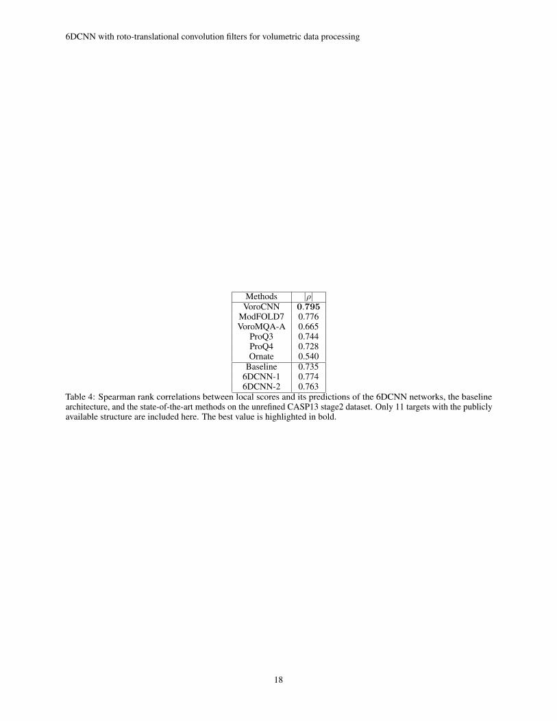
Table 4 lists Spearman rank correlations of local quality predictions with the corresponding ground-truth values of ourthree networks and the state-of-the-art methods on model structures of 11 targets from CASP13. For the comparison,we chose only model structures that had both publicly available target structures and predictions of local scores fromother methods.

17


Methods |ρ|VoroCNN 0.795

ModFOLD7 0.776VoroMQA-A 0.665

ProQ3 0.744ProQ4 0.728Ornate 0.540

Baseline 0.7356DCNN-1 0.7746DCNN-2 0.763

Table 4: Spearman rank correlations between local scores and its predictions of the 6DCNN networks, the baselinearchitecture, and the state-of-the-art methods on the unrefined CASP13 stage2 dataset. Only 11 targets with the publiclyavailable structure are included here. The best value is highlighted in bold.

18

6dcnn with roto-translational convolution filters - archive

Documents