SOME APPLICATIONS OF THE SOME APPLICATIONS OF THE CONVOLUTION AND KRONECKER CONVOLUTION AND KRONECKER

PRODUCTS OF MATRICES PRODUCTS OF MATRICES

ByBy

ZeyadZeyad Al Al ZhourZhour and and AdemAdem KilicmanKilicman

OBJECTIVESOBJECTIVES

To establish some properties of the CP and KCP that will To establish some properties of the CP and KCP that will be useful in our investigation of the solution of matrix and be useful in our investigation of the solution of matrix and matrix differential equations.matrix differential equations.

To present the general vectorTo present the general vector--operator solutions of coupledoperator solutions of coupledmatrix differential equationsmatrix differential equations

To present the general vectorTo present the general vector--operator solutions of generaloperator solutions of generalcoupled matrix convolution differential equations.coupled matrix convolution differential equations.

Some special cases of these systems are also Some special cases of these systems are also considereconsidereand solved. and solved.

INTRODUCTIONINTRODUCTIONMatrix and matrix differential equations have been widely used iMatrix and matrix differential equations have been widely used in stability n stability theory, control theory, system theory, communication systems andtheory, control theory, system theory, communication systems and other other fields of pure and applied mathematics.fields of pure and applied mathematics.

There are some papers devoted to the analysis, existence, uniqueThere are some papers devoted to the analysis, existence, uniqueness ness and representation of the solution and also to the numerical algand representation of the solution and also to the numerical algorithm to orithm to solve various types of matrix equations.solve various types of matrix equations.

For example:For example:

NikolaosNikolaos ((19971997) presented a new method to obtain closed form solutions ) presented a new method to obtain closed form solutions of transition probabilities and dependability measures and then of transition probabilities and dependability measures and then solved the solved the renewal matrix equation by using the convolution product of matrrenewal matrix equation by using the convolution product of matrices.ices.

SumitaSumita ((19841984) established the matrix ) established the matrix LaguerreLaguerre transform to calculatetransform to calculatematrix convolutions and evaluated a matrix renewal functionmatrix convolutions and evaluated a matrix renewal function..

Fulton and WuFulton and Wu ((19971997) presented the solution of the (full ) presented the solution of the (full rank) least square problem: by rank) least square problem: by QRQR, , LULU and and SVDSVDapproaches.approaches.

Ding and ChenDing and Chen (2005(2005) presented the new iterative methods ) presented the new iterative methods to solve coupled Sylvester matrix equations.to solve coupled Sylvester matrix equations.

bxBA ≈⊗ )(

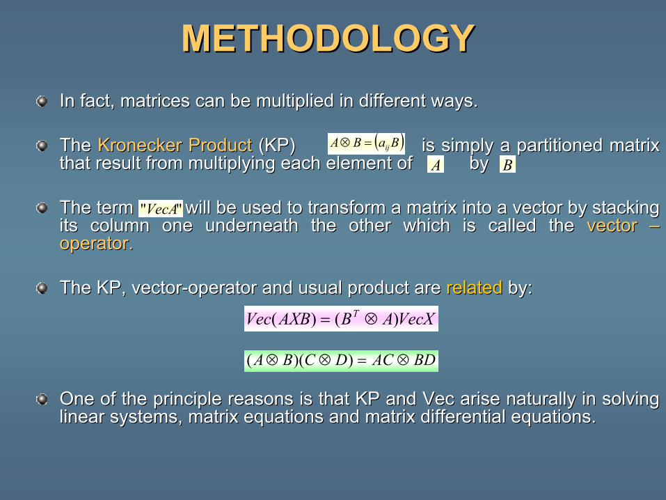
METHODOLOGYMETHODOLOGYIn fact, matrices can be multiplied in different ways. In fact, matrices can be multiplied in different ways.

The The KroneckerKronecker ProductProduct (KP) is simply a partitioned matrix (KP) is simply a partitioned matrix that result from multiplying each element of bythat result from multiplying each element of by

The term will be used to transform a matrix into a vectThe term will be used to transform a matrix into a vector by stacking or by stacking its column one underneath the other which is called the its column one underneath the other which is called the vector vector ––operator.operator.

The KP, vectorThe KP, vector--operator and usual product are operator and usual product are relatedrelated by:by:

One of the principle reasons is that KP and One of the principle reasons is that KP and VecVec arise naturally in solving arise naturally in solving linear systems, matrix equations and matrix differential equatiolinear systems, matrix equations and matrix differential equations.ns.

( )BaBA ij=⊗

A B

""VecA

VecXABAXBVec T )()( ⊗=

BDACDCBA ⊗=⊗⊗ ))((

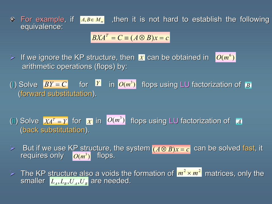
For exampleFor example, if ,then it is not hard to establish the following , if ,then it is not hard to establish the following equivalence:equivalence:

If we ignore the KP structure, then can be obtained inIf we ignore the KP structure, then can be obtained inarithmetic operations (flops) by:arithmetic operations (flops) by:

((II) Solve for in flops usi) Solve for in flops using ng LULU factorization of factorization of ((forward forward substitutationsubstitutation).).

((iiii) Solve for in flops using ) Solve for in flops using LULU factorization of factorization of ((back back substitutationsubstitutation).).

But if we use KP structure, the system can But if we use KP structure, the system can be solved be solved fastfast, it , it requires only flops.requires only flops.

The KP structure also a voids the formation of matThe KP structure also a voids the formation of matrices, only the rices, only the smaller are needed.smaller are needed.

cxBACBXAT =⊗≡= )(

X )( 6mO

CBY = )( 3mO

X )( 3mOYXAT =

Y B

A

cxBA =⊗ )()( 3mO

22 mm ×BABA UULL ,,,

mMBA ∈,

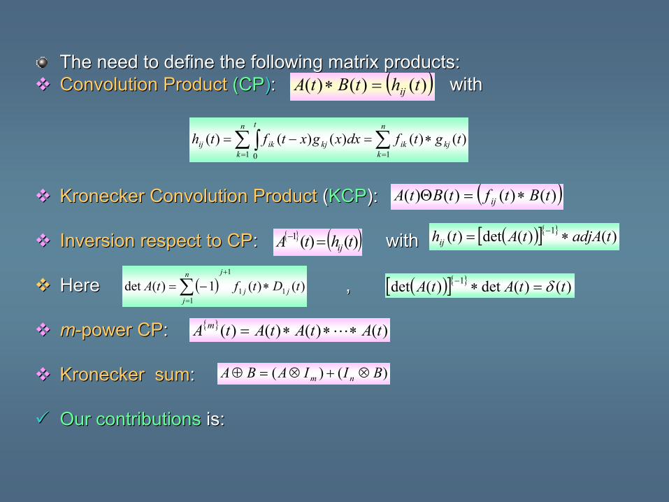
The need to define the following matrix products:The need to define the following matrix products:Convolution ProductConvolution Product (CP(CP)): with: with

KroneckerKronecker Convolution ProductConvolution Product ((KCPKCP):):

Inversion respect to CPInversion respect to CP: with: with

Here ,Here ,

mm--power CPpower CP: :

KroneckerKronecker sumsum: :

Our contributionsOur contributions is: is:

( ))()()( thtBtA ij=∗

)()()()()(11 0

tgtfdxxgxtfth kj

n

kik

n

k

t

kjikij ∗=−= ∑∑∫==

( ))()()()( tBtftBtA ij ∗=Θ

{ } ( ))()(1 thtA ij=− ( )[ ]{ } )()(det)( 1 tadjAtAthij ∗= −

( ) )()(1)(det 11

1

1tDtftA jj

jn

j∗−=

+

=∑ ( )[ ]{ } )()(det)(det 1 ttAtA δ=∗−

{ } )()()()( tAtAtAtA m ∗∗∗= L

)()( BIIABA nm ⊗+⊗=⊕

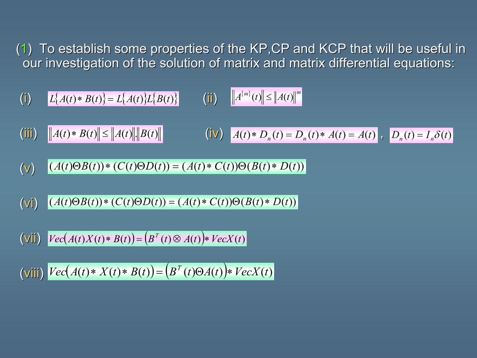
((11) To establish some properties of the KP,CP and KCP that will b) To establish some properties of the KP,CP and KCP that will be useful in e useful in our investigation of the solution of matrix and matrix differentour investigation of the solution of matrix and matrix differential equations:ial equations:

((ii) () (iiii) )

((iiiiii) () (iviv) , ) ,

((vv) )

((vivi) )

((viivii) )

((viiiviii))

{ } { } { })()()()( tBLtALtBtAL =∗

))()(())()(())()(())()(( tDtBtCtAtDtCtBtA ∗Θ∗=Θ∗Θ

))()(())()(())()(())()(( tDtBtCtAtDtCtBtA ∗Θ∗=Θ∗Θ

{ } mm tAtA )()( ≤

( ) ( ) )()()()()()( tVecXtAtBtBtXtAVec T ∗⊗=∗

( ) ( ) )()()()()()( tVecXtAtBtBtXtAVec T ∗Θ=∗∗

)(.)()()( tBtAtBtA ≤∗ )()()()()( tAtAtDtDtA nn =∗=∗ )()( tItD nn δ=

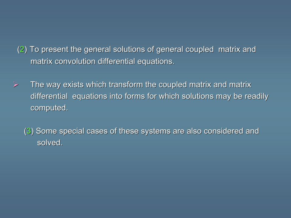
((22)) To present the general solutions of general coupled matrix and To present the general solutions of general coupled matrix and matrix convolution differential equations.matrix convolution differential equations.

The way exists which transform the coupled matrix and matrix The way exists which transform the coupled matrix and matrix differential equations into forms for which solutions mdifferential equations into forms for which solutions may be readilyay be readilycomputed. computed.

((33) Some special cases of these systems are also considered and) Some special cases of these systems are also considered andsolved. solved.

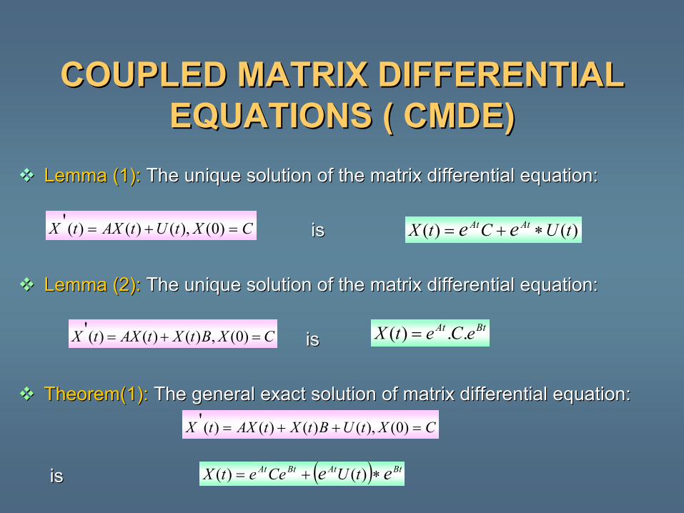
Lemma (1):Lemma (1): The unique solution of the matrix differential equation:The unique solution of the matrix differential equation:

isis

Lemma (2):Lemma (2): The unique solution of the matrix differential equation:The unique solution of the matrix differential equation:

isis

Theorem(1):Theorem(1): The general exact solution of matrix differential equation:The general exact solution of matrix differential equation:

is is

COUPLED MATRIX DIFFERENTIAL COUPLED MATRIX DIFFERENTIAL EQUATIONS ( CMDE)EQUATIONS ( CMDE)

CXBtXtAXtX =+= )0(,)()()(' BtAt eCetX ..)( =

CXtUtAXtX =+= )0(),()()(' )()( tUCtX AtAt ee ∗+=

CXtUBtXtAXtX =++= )0(),()()()('

( ) BtAtBtAt ee tUCeetX ∗+= )()(

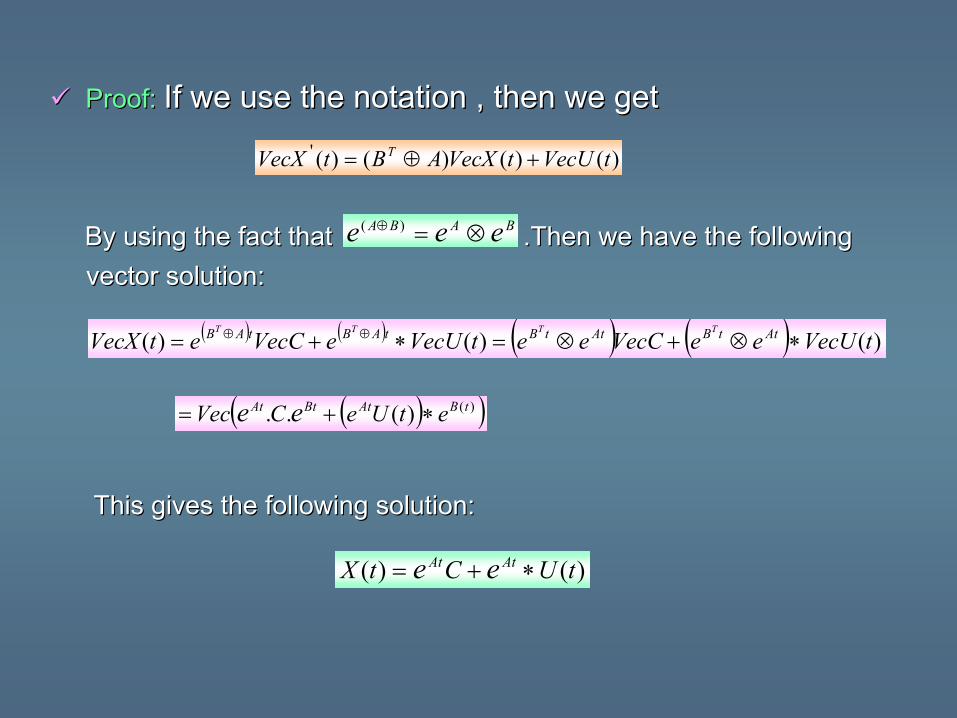
Proof:Proof: If we use the notation , then we getIf we use the notation , then we get

By using the fact that .Then we have thBy using the fact that .Then we have the following e following vector solution:vector solution:

This gives the following solution: This gives the following solution:

)()()()(' tVecUtVecXABtVecX T +⊕=

( ) ( ) ( ) ( ) )()()( tVecUeeVecCeetVecUeVecCetVecX AttBAttBtABtAB TTTT

∗⊗+⊗=∗+= ⊕⊕

BABA eee ⊗=⊕ )(

( )( ))()(.. tBAtBtAt etUeCVec ee ∗+=

)()( tUCtX AtAt ee ∗+=

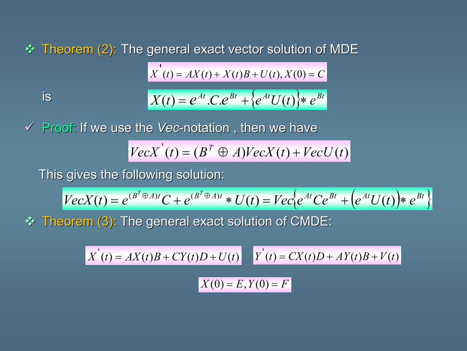
Theorem (2):Theorem (2): The general exact vector solution of MDEThe general exact vector solution of MDE

is is

Proof:Proof: If we use the If we use the VecVec--notation , then we have notation , then we have

This gives the following solution:This gives the following solution:

Theorem (3):Theorem (3): The general exact solution of CMDE:The general exact solution of CMDE:

CXtUBtXtAXtX =++= )0(),()()()('

{ } BtAtBtAt etUeCtX ee ∗+= )(..)(

)()()()(' tVecUtVecXABtVecX T +⊕=

( ){ }BtAtBtAttABtAB etUeCeeVectUeCetVecXTT

∗+=∗+= ⊕⊕ )()()( )()(

)()()()(' tUDtCYBtAXtX ++= )()()()(' tVBtAYDtCXtY ++=

FYEX == )0(,)0(

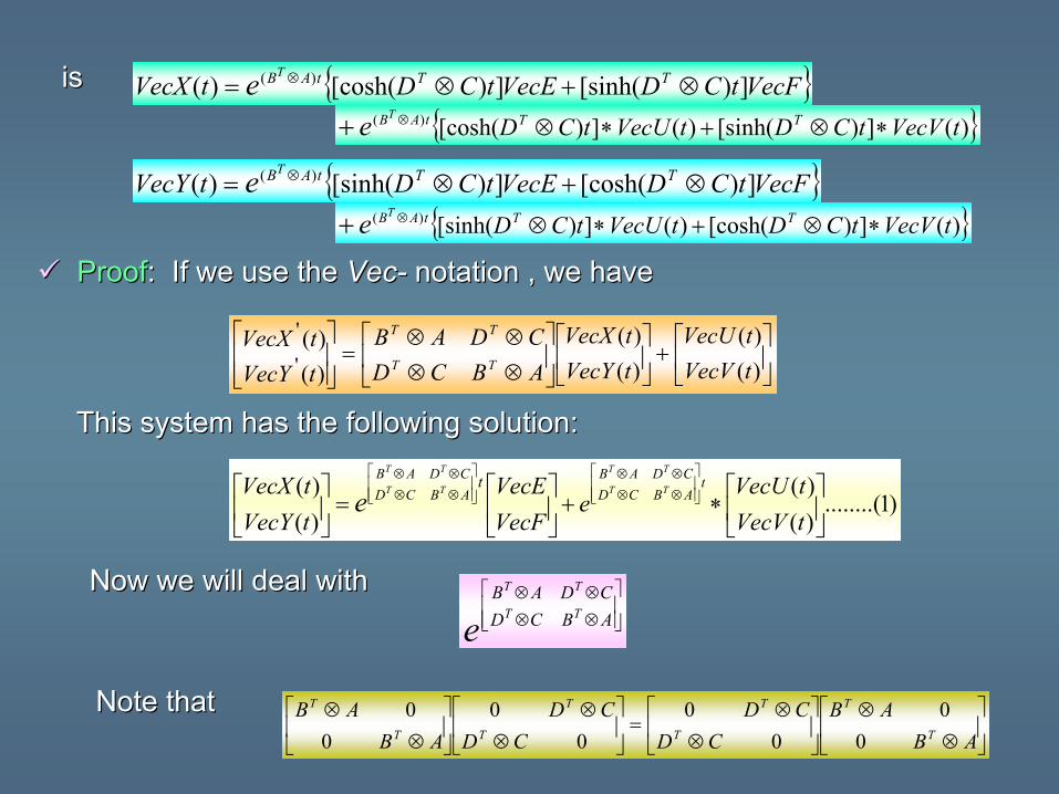
isis

ProofProof: If we use the : If we use the VecVec-- notation , we havenotation , we have

This system has the following solution:This system has the following solution:

Now we will deal withNow we will deal with

Note thatNote that

{ }VecFtCDVecEtCDtVecX TTtABTe ])[sinh(])[cosh()( )( ⊗+⊗= ⊗

{ })(])[sinh()(])[cosh()( tVecVtCDtVecUtCD TTtABTe ∗⊗+∗⊗⊗+

{ }VecFtCDVecEtCDtVecY TTtABTe ])[cosh(])[sinh()( )( ⊗+⊗= ⊗

{ })(])[cosh()(])[sinh()( tVecVtCDtVecUtCD TTtABTe ∗⊗+∗⊗⊗+

+

⊗⊗⊗⊗

=

)()(

)()(

)()(

'

'

tVecVtVecU

tVecYtVecX

ABCDCDAB

tVecYtVecX

TT

TT

)1........()()(

)()(

∗+

=

⊗⊗⊗⊗

⊗⊗⊗⊗

tVecVtVecU

eVecFVecE

tVecYtVecX t

ABCDCDAB

ABCDCDAB

TT

TT

TT

TTt

e

⊗⊗⊗⊗ABCDCDAB

TT

TT

e

⊗⊗

⊗⊗

=

⊗⊗

⊗⊗

ABAB

CDCD

CDCD

ABAB

T

T

T

T

T

T

T

T

00

00

00

00

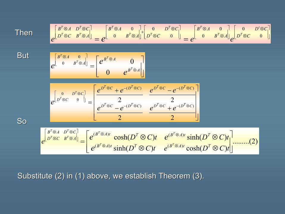
ThenThen

ButBut

SoSo

Substitute (2) in (1) above, we establish Theorem (3).Substitute (2) in (1) above, we establish Theorem (3).

⊗⊗

⊗⊗

⊗⊗

+

⊗⊗

⊗⊗⊗⊗

== 00

00

00

00

CDCD

ABAB

CDCD

ABAB

ABCDCDAB

T

t

T

T

T

T

T

T

TT

TT

eee e

=

⊗

⊗

⊗⊗

AB

ABAB

AB

T

TT

T

eee0

000

+−

−+

=⊗−⊗⊗−⊗

⊗−⊗⊗−⊗

⊗⊗

22

22)()(

)()(

00

CDCDCDCD

CDCDCDCD

CDCD

TTTT

TTTT

eeee

eeeeT

T

e

)2.........()cosh()sinh()sinh()cosh(

)()(

)()(

⊗⊗⊗⊗=

⊗⊗

⊗⊗

⊗⊗⊗⊗

tCDetCDtCDtCDe

TtABTtAB

TtABTtABABCDCDAB

TT

TTTT

TT

eee

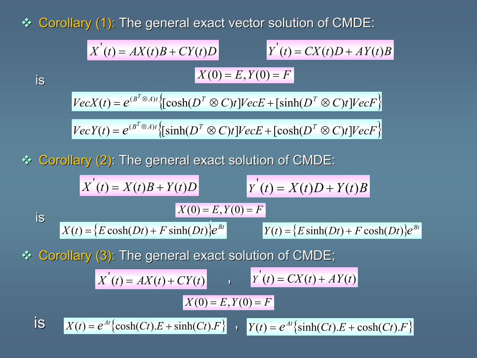
Corollary (1):Corollary (1): The general exact vector solution of CMDE: The general exact vector solution of CMDE: ,,

is is

Corollary (2)Corollary (2): The general exact solution of CMDE:: The general exact solution of CMDE:,,

is ,is ,

Corollary (3):Corollary (3): The general exact solution of CMDE;The general exact solution of CMDE;

,,

is ,is ,

DtCYBtAXtX )()()(' += BtAYDtCXtY )()()(' +=

FYEX == )0(,)0(

{ }VecFtCDVecEtCDtVecX TTtABTe ])[sinh(])[cosh()( )( ⊗+⊗= ⊗

{ }VecFtCDVecEtCDtVecY TTtABTe ])[cosh(])[sinh()( )( ⊗+⊗= ⊗

DtYBtXtX )()()(' += BtYDtXtY )()()(' +=

FYEX == )0(,)0(

{ } BteDtFDtEtX )sinh()cosh()( += { } BteDtFDtEtY )cosh()sinh()( +=

)()()(' tCYtAXtX += )()()(' tAYtCXtY +=

FYEX == )0(,)0(

{ }FCtECttX Ate ).sinh().cosh()( += { }FCtECttY Ate ).cosh().sinh()( +=

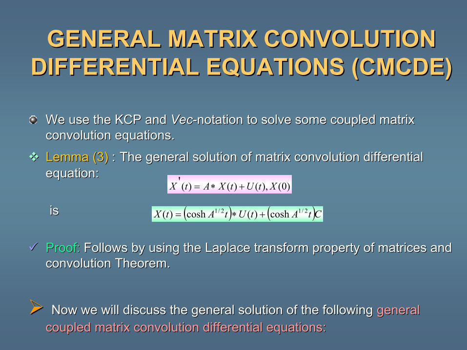
GENERAL MATRIX CONVOLUTION GENERAL MATRIX CONVOLUTION DIFFERENTIAL EQUATIONS (CMCDE)DIFFERENTIAL EQUATIONS (CMCDE)

We use the KCP and We use the KCP and VecVec--notation to solve some coupled matrix notation to solve some coupled matrix convolution equations.convolution equations.

Lemma (3)Lemma (3) :: The general solution of matrix convolution differential The general solution of matrix convolution differential equation: equation:

is is

Proof:Proof: Follows by using the Follows by using the LaplaceLaplace transform property of matrices and transform property of matrices and convolution Theorem.convolution Theorem.

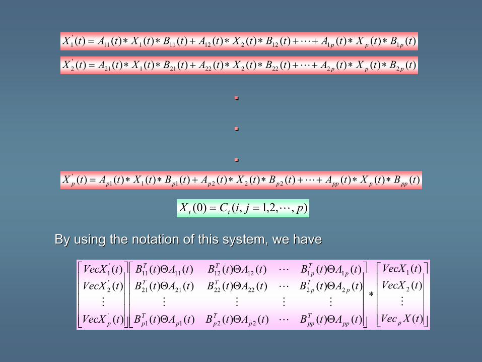
Now weNow we willwill discuss the general solution of the following discuss the general solution of the following general general coupled matrix convolution differential equations:coupled matrix convolution differential equations:

)0(),()()(' XtUtXAtX +∗=

( ) ( )CtAtUtAtX 2/12/1 cosh)(cosh)( +∗=

..

..

..

By using the notation of this system, we have By using the notation of this system, we have

)()()()()()()()()()( 111221211111'1 tBtXtAtBtXtAtBtXtAtX ppp ∗∗++∗∗+∗∗= L

)()()()()()()()()()( 222222221121'2 tBtXtAtBtXtAtBtXtAtX ppp ∗∗++∗∗+∗∗= L

)()()()()()()()()()( 222111' tBtXtAtBtXtAtBtXtAtX pppppppppp ∗∗++∗∗+∗∗= L

),,2,1,()0( pjiCX ii L==

∗

ΘΘΘ

ΘΘΘΘΘΘ

)(

)()(

)()()()()()(

)()()()()()()()()()()()(

)(

)()(

2

1

2211

2222222121

1112121111

'

'2

'1

tXVec

tVecXtVecX

tAtBtAtBtAtB

tAtBtAtBtAtBtAtBtAtBtAtB

tVecX

tVecXtVecX

pppTppp

Tpp

Tp

pTp

TTp

Tp

TT

p

M

L

MMMM

L

L

M

This system can rewrite as This system can rewrite as

If we use If we use LaplaceLaplace transform, we have transform, we have

Here,Here,

By taking By taking LaplaceLaplace inverse of both side of (1), we haveinverse of both side of (1), we have

Here, .Here, .

Now, can be obtained by two ways, eitheNow, can be obtained by two ways, either by truncated r by truncated series development or by explicit inversion within the above desseries development or by explicit inversion within the above described cribed convolution algebra. convolution algebra.

cxtxtHtx =∗= )0(),()()('

( ){ } )1..().........(,()( 1 sGsIcsGsIsY >−= −

{ } { })()(,)()( tHLsGtxLsY ==

{ }

( ){ } )2(....................)()(1)( 11

1 ctQIIcssGI

sLtx −

−− −∗=

−=

)()( tHItQ ∗=

( ){ }1)( −− tQI

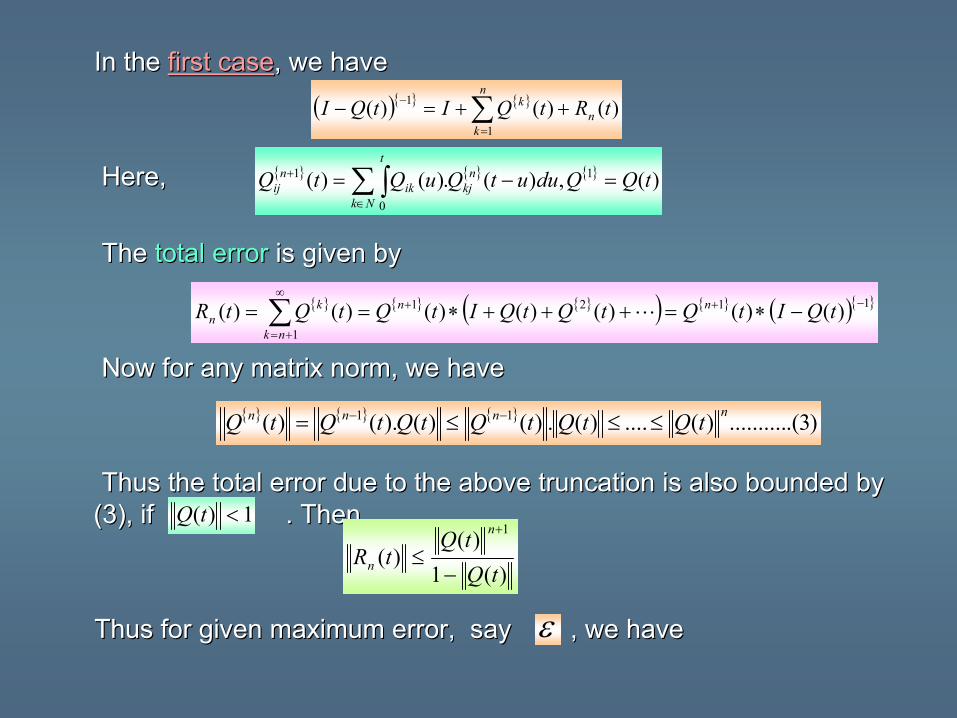
In the In the first casefirst case, we have , we have

Here, Here,

The The total errortotal error is given byis given by

Now for any matrix norm, we have Now for any matrix norm, we have

Thus the total error due to the above truncation is also bThus the total error due to the above truncation is also bounded by ounded by (3), if . Then(3), if . Then

Thus for given maximum error, say , we have Thus for given maximum error, say , we have

( ){ } { } )()()(1

1 tRtQItQI n

n

k

k ++=− ∑=

−

{ } { } { } )(,)(.)()( 1

0

1 tQQduutQuQtQ nkj

Nk

t

iknij =−= ∑∫

∈

+

{ } { } { }( ) { } ( ){ }11

1

21 )()()()()()()( −+∞

+=

+ −∗=+++∗== ∑ tQItQtQtQItQtQtR n

nk

nkn L

{ } { } { } )3.(..........)(....)(.)()().()( 11 nnnn tQtQtQtQtQtQ ≤≤≤= −−

1)( <tQ

)(1)(

)(1

tQtQ

tRn

n −≤

+

ε

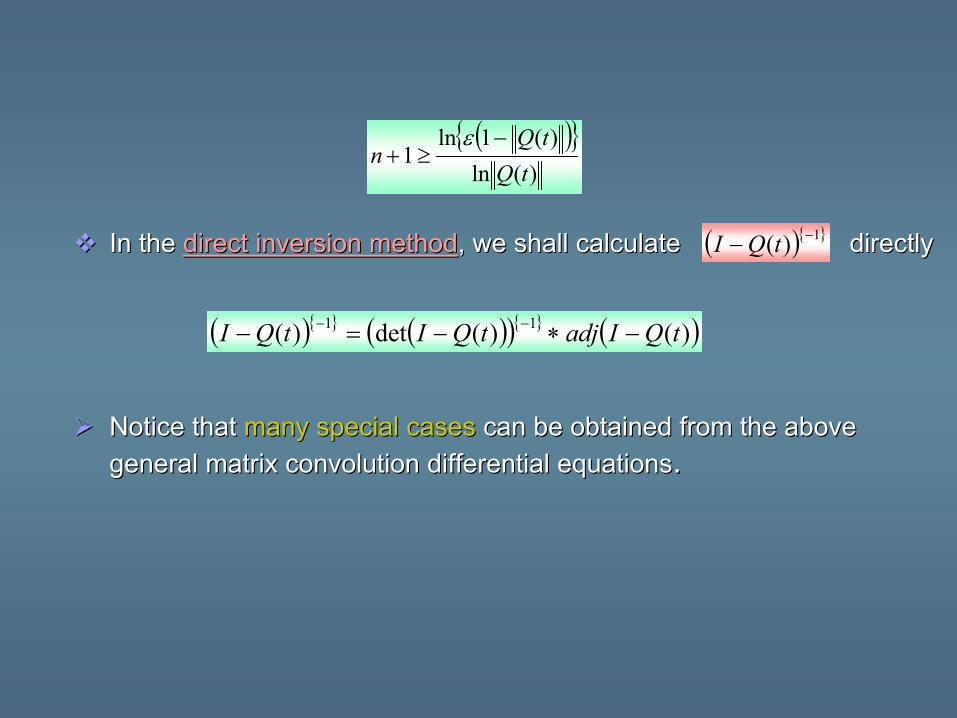
In the In the direct inversion methoddirect inversion method, we shall calculate directly, we shall calculate directly

Notice that Notice that many special casesmany special cases can be obtained from the above can be obtained from the above general matrix convolution differential equationsgeneral matrix convolution differential equations..

( ){ })(ln)(1ln

1tQtQ

n−

≥+ε

( ){ }1)( −− tQI

( ){ } ( )( ){ } ( ))()(det)( 11 tQIadjtQItQI −∗−=− −−

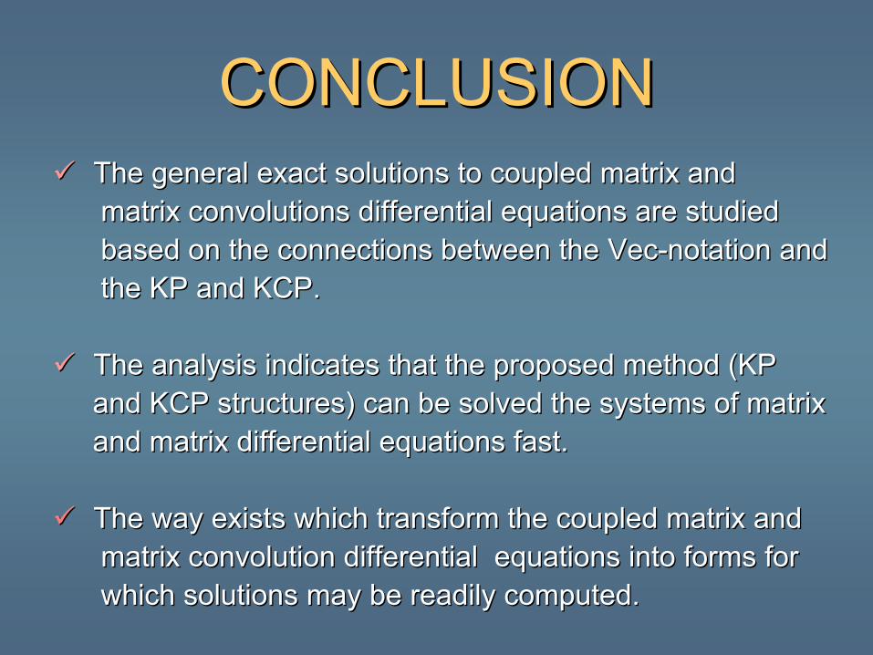
CONCLUSIONCONCLUSIONThe general exact solutions to coupled matrix andThe general exact solutions to coupled matrix andmatrix convolutions differential equations are studiedmatrix convolutions differential equations are studiedbased on the connections between the based on the connections between the VecVec--notation andnotation andthe KP and KCP.the KP and KCP.

The analysis indicates that the proposed method (KP The analysis indicates that the proposed method (KP and KCP structures) can be solved the systems of matrixand KCP structures) can be solved the systems of matrixand matrix differential equations fast. and matrix differential equations fast.

The way exists which transform the coupled matrix and The way exists which transform the coupled matrix and matrix convolution differential equations into forms formatrix convolution differential equations into forms forwhich solutions may be readily computed. which solutions may be readily computed.

The KP structure is easy to understand, simple to useThe KP structure is easy to understand, simple to useand accurate. and accurate.

How to use the KP and KCP structures to solve the nonHow to use the KP and KCP structures to solve the non--linear matrix and matrix convolution differential equations linear matrix and matrix convolution differential equations require research.require research.