time-domain impedance formulation based on recursive convolution
TRANSCRIPT
Time-Domain Impedance Formulation based on
Recursive Convolution
Yves Reymen∗, Martine Baelmans†, and Wim Desmet.†
Katholieke Universiteit Leuven, Department of Mechanical Engineering, Leuven, Belgium
In many aeroacoustic applications lining material plays an important role in controllingthe emitted noise levels. To be able to study the effect of different materials and tojudge their effectiveness, adequate numerical models are essential in the design process.They enable the optimization of noise reduction through sensitivity analyses of the variousmaterial and geometrical system parameters.
The acoustic characterization of lining material is commonly done in the frequency-domain, through the impedance that relates the pressure to the normal velocity. Theimpedance is typically provided as a list of complex values at some discrete frequencies.In order to incorporate lining material models in a time-domain calculation scheme, some‘translation’ of the impedance into the time domain is needed.
This contribution describes a new impedance boundary condition, suited for single fre-quency as well as for broadband simulations in the time-domain. First, a continuous fre-quency model is generated through curvefitting the sampled impedance values using pre-defined frequency templates having a priori known time domain counterparts. Secondly,the time domain formulation is obtained by recursive convolution, performed in a novelway using (complex-valued) accumulators.
The impedance formulation is suited for general broadband simulations because it em-beds sufficient freedom to make a good fit to the sampled impedance values. The recursiveconvolutions makes the formulation very efficient as it requires only a few additions andmultiplications. It doesn’t require solution data from previous time steps to be stored orhigh order time derivatives as did some previous formulations.
The formulation is implemented within the framework of a Quadrature-Free Discon-tinuous Galerkin Method for the Linearized Euler Equations. As a first validation, it isapplied to a semi-infinite two-dimensional duct with a hard upper and an acousticallytreated lower wall, for which an analytical solution exists. Further validation was done bycomparing numerical results with measurement data for the NASA Langley flow impedancetube (TP-2679), a well documented benchmark. For both single frequency and broadbandsimulations, with and without mean flow, some good agreement with experimental data isobtained.
I. Introduction
In many aeroacoustic applications lining material plays an important role in controlling the emitted noiselevels. To be able to study the effect of different materials and to judge their effectiveness, adequate numericalmodels are essential. Optimization of the noise reduction becomes possible by numericla sensitivity analysesof the various material parameters and the geometrical layout.
Most often, lining material is acoustically characterized in the frequency-domain. This is usually doneby setting up a test with a single harmonic wave excitation and identifying the impedance from the forcedresponse. The obtained complex value is the impedance at the frequency of the harmonic wave excitation.This procedure can only describe linear effects.
Time-domain computational methods have a clear advantage over frequency-domain methods for broad-band problems, non-linear interaction investigations and transient wave simulations. To be able to represent
∗PhD Student, [email protected], AIAA student member.†Professor, Dept. of Mechanical Engineering, Celestijnenlaan 300, B-3001 Heverlee, Belgium.
1 of 14
American Institute of Aeronautics and Astronautics
12th AIAA/CEAS Aeroacoustics Conference (27th AIAA Aeroacoustics Conference)8 - 10 May 2006, Cambridge, Massachusetts
AIAA 2006-2685
Copyright © 2006 by Y. Reymen, M. Baelmans and W. Desmet. Published by the American Institute of Aeronautics and Astronautics, Inc., with permission.
an impedance boundary in the time-domain, there is a need to ‘translate’ the frequency data to the time-domain.
At a given frequency ω, the pressure P (xb, ω) in the frequency-domain for a position xb on the liningmaterial, is proportional to the normal velocity V (xb, ω) by the impedance Z(ω). A capital indicates theFourier transform of a quantity. The equivalent expression in the time-domain involves the convolution ofthe inverse Fourier transform z(t) of the impedance with the velocity.1
P (xb, ω) = Z(ω) · V (xb, ω) (1)
p(xb, t) = z(t) ∗ v(xb, t) =∫ ∞−∞
z(τ) · v(xb, t− τ)dτ (2)
To be able to take the inverse Fourier transform of the impedance, equation (3), Z has to be known overthe entire frequency range. This extension to all possible frequencies poses a first difficulty and establishesthe need for an impedance model. Secondly the convolution has to be performed, which, in its full form, isa very costly operation (in terms of CPU time), and, in addition it requires the entire time history of thevelocity.
z(t) =∫ ∞−∞
Z(ω)eiωtdω (3)
For an impedance model to be physically feasible, it has to comply with 3 necessary conditions as indicatedby Rienstra.1 It has to be causal, real and passive. These conditions are not trivially satisfied by a generalpolynomial fit to the frequency data. Fortunately, the second difficulty, the full convolution, can be avoidedin many ways. These include, without going into further details, replacing iω by d/dt, the z-transform, andrecursive convolution.
Tam & Aurialt2 proposed a 3-parameter model, resembling a mass-spring-damper system, and replacediω by d/dt. This leads to a formulation with very low computational cost, but it is not applicable as a generalbroadband model. Ozyoruk3 proposed a broadband impedance model based on a rational polynomial fitin combination with the z-transform. This model is rather sensitive to instabilities, but can be used as ageneral broadband model. Rienstra1 proposed a model based on a Helmholtz-resonator and the z-transformthat satifies all conditions and can be exactly tuned to the impedance at a design frequency. Fung &Ju4 proposed a model for the reflection coefficient, relating incoming and outgoing velocities. This enablesto apply a space-time continuation that allows for a non-causal model. The convolution is dealt with byrecursion, an idea originally developed in the computational electromagnetics community.
The goal of this research is to develop a time-domain impedance formulation that is suited for generalbroadband simulations. This formulation is to be incorporated in a Quadrature-Free Discontinous GalerkinMethod for the Linearized Euler Equations.9 A single-frequency formulation, that can be tuned to any givenimpedance value at a design frequency, is also developed.
As a first validation case, a 2D duct is studied with a hard and a soft wall excited by a single frequencyand without mean flow. For this case an analytical reference solution is known.11 The formulation startsfrom a causal, real, and passive second-order admittance model in the frequency-domain and fits this to thecomplex valued impedance at the given frequency. The time-domain formulation is obtained by a novel wayto perform recursive convolution. This only needs to store some data in accumulators, it doesn’t need anytime derivatives or storage of the solution at previous timesteps.
Further validation of the formulation is done for the NASA Langley Flow Impedance Tube.6 This is awell-documented benchmark that includes cases with and without mean flow for 6 frequencies. It allowsto test the single frequency formulation by simulating only one frequency in each simulation as well as thebroadband formulation by exciting the tube with multiple frequencies. The broadband formulation modelsthe impedance/admittance in the frequency-domain as the sum of first- and/or second-order systems anduses the same efficient recursive convolution procedure.
II. Impedance Modelling
Although the time-domain allows the description of non-linear effects,5 models are limited here to linearinteractions as a frequency-domain impedance model is used as starting point.
Looking back to equation (2), z(t) can be viewed in terms of linear systems theory as the unit impulseresponse of the system Z(ω).5 If the system can be described by a rational function of which the order of
2 of 14
American Institute of Aeronautics and Astronautics
the polynomial in the numerator is smaller than that in the denominator, it can be written in the form of apartial fraction expansion with residues Ak and poles pk, equation (4), similar to the model of Fung & Jufor the reflection coefficient.4
Z(ω) =P∑
k=1
Ak
iω + pk(4)
If the order of the numerator is higher than that of the denominator, one can work with the admittance,the inverse of the impedance. The only thing that changes in the formulation is the switch of position ofpressure and velocity. If the order of the numerator and that of the denominator are equal, there is an extraconstant term in the general model, which is trivial to incorporate.
The poles have to be real λ or complex conjugated α ± iβ for z(t) to be real. Each real pole deter-mines a first-order system (5), each pair of complex conjugated poles determines a second-order system (7).Equations (6) and (8) give their corresponding unit impulse responses.
Zk(ω) =Ak
iω + λk(5)
zk(t) = Ake−λktH(t) λk ≥ 0 (6)
Zl(ω) =A2l−1
iω + p2l−1+
A2l
iω + p2l=
Cl(iω) +Dl
(iω + αl)2 + β2l
(7)
zl(t) = e−αlt
(Cl cos(βlt) +
Dl − αlCl
βlsin(βlt)
)H(t) αl ≥ 0 (8)
The condition λk ≥ 0 and αl ≥ 0 is to ensure causality of z(t). H(t) is the Heaviside function.
A. Broadband Model
A general impedance model can be written as the sum of S single pole systems and T complex conjugatepair systems. It can be easily shown that it is causal and real. For a good choice of the parameters it is alsopassive.
Z(ω) =S∑
k=1
Ak
iω + λk+
T∑l=1
Cl(iω) +Dl
(iω + αl)2 + β2l
λk ≥ 0 & αl ≥ 0 (9)
=S∑
k=1
Zk(ω) +T∑
l=1
Zl(ω) (10)
z(t) =S∑
k=1
zk(t) +T∑
l=1
zl(t) (11)
B. Time-Domain Formulation
The convolution of the impedance impulse response z(t) with the velocity v(t), equation (2), can be calculatedby recursive convolution thanks to the special form of zk(t) and zl(t) and the assumption that the velocityis piecewise constant or piecewise linear within a timestep ∆t. The derivation is inspired by the work ofLuebbers.7,8
1. Preliminary considerations
The expression of zl(t), equation (8), can be simplified by defining the constants K1l and K2l. Application ofEuler’s formula for complex numbers allows to write it in a more convenient form, similar to the expressionfor zk(t), equation (6).
zl(t) = e−αlt
(Cl cos(βlt) +
Dl − αlCl
βlsin(βlt)
)H(t) (12)
= e−αlt (K1l cos(βlt) +K2l sin(βlt))H(t) (13)
=(K1l ·Re{e(−α+iβ)t}+K2l · Im{e(−α+iβ)t}
)H(t) (14)
3 of 14
American Institute of Aeronautics and Astronautics
Re{·} and Im{·} are, respectively, the real and imaginary part.The normal velocity is approximated as piecewise linear within a timestep ∆t. For the recursive con-
volution, it is necessary to write that approximation as a function of the reverse time that is also shiftedby τ .
vn(t) = vin +
vi+1n − vi
n
∆t(t− i∆t) for t ∈ [i∆t, (i+ 1)∆t] (15)
vn(n∆t− τ) = vn−mn +
vn−m−1n − vn−m
n
∆t(τ −m∆t) for τ ∈ [m∆t, (m+ 1)∆t] (16)
2. Recursive Convolution
The derivation of the recursive convolution starts from equation (2) that gives the pressure as the convolutionof the impulse response of the impedance with the normal velocity. The first step is to write that in a discreteform and replace the integral over the past time as a sum of integrals over intervals, each the size of onetime step.
p(xb, t) = z(t) ∗ v(xb, t) =∫ ∞−∞
z(τ) · v(xb, t− τ)dτ (2)
p(n∆t) =∫ n∆t
0
z(τ) · v(n∆t− τ)dτ =n−1∑m=0
∫ (m+1)∆t
m∆t
z(τ) · v(n∆t− τ)dτ (17)
Substitution of the general impedance model (11) and the piecewise linear approximation of the normalvelocity (16) in equation (17) gives
p(n∆t) =n−1∑m=0
∫ (m+1)∆t
m∆t
(S∑
k=1
zk(τ) +T∑
l=1
zl(τ)
)·(vn−m
n +vn−m−1
n − vn−mn
∆t(τ −m∆t)
)dτ (18)
Using the definitions
χmk =
∫ (m+1)∆t
m∆t
e−λkτdτ, ξmk =
1∆t
∫ (m+1)∆t
m∆t
(τ −m∆t)e−λkτdτ, (19)
χ̂ml =
∫ (m+1)∆t
m∆t
e(−αl+iβl)τdτ and ξ̂ml =
1∆t
∫ (m+1)∆t
m∆t
(τ −m∆t)e(−αl+iβl)τdτ (20)
and changing the order of the summations, equation (18) becomes
p(n∆t) =S∑
k=1
Ak
n−1∑m=0
(vn−m
n χmk + (vn−m−1
n − vn−mn )ξm
k
)· · ·
+T∑
l=1
(K1lRe
{n−1∑m=0
(vn−m
n χ̂ml + (vn−m−1
n − vn−mn )ξ̂m
l
)}· · ·
+K2lIm
{n−1∑m=0
(vn−m
n χ̂ml + (vn−m−1
n − vn−mn )ξ̂m
l
)})(21)
Real-valued auxilary variable ψk is defined as the result of the first summation over m in (21). Sim-ilarly, a complex-valued ψ̂l is defined as the second or third summation over m, the two being identi-cal. These variables are accumulators, that can be recursively updated because χm+1
k = e−λk∆tχmk and
χ̂m+1l = e(−αl+iβl)∆tχ̂m
l and likewise for ξk and ξ̂l. A proof is given in the appendix.The resulting formulation of the time-domain impedance using recursive convolution and a piecewise
4 of 14
American Institute of Aeronautics and Astronautics

linear approximation of the normal velocity is given by
ψk(n∆t) =v(n∆t)1− e−λk∆t
λk+ (v((n− 1)∆t)− v(n∆t))
e−λkt(−λk∆t− 1) + 1λ2
k∆t+ ψk((n− 1)∆t)e−λk∆t
(22)
ψ̂l(n∆t) =v(n∆t)1− e(−αl+iβl)∆t
αl − iβl+ (v((n− 1)∆t)− v(n∆t))
e(−αl+iβl)t((−αl + iβl)∆t− 1) + 1(−αl + iβl)2∆t
+ ψ̂l((n− 1)∆t)e(−αl+iβl)∆t (23)
p(n∆t) =S∑
k=1
Akψk(n∆t) +T∑
l=1
Cl ·Re{ψ̂l(n∆t)}+Dl − αlCl
βl· Im{ψ̂l(n∆t)} (24)
If a piecewise constant velocity approximation is used, the update equations for ψk and ψ̂l are
ψk(n∆t) = v(n∆t)1− e−λk∆t
λk+ ψk((n− 1)∆t)e−λk∆t (25)
ψ̂l(n∆t) = v(n∆t)1− e(−αl+iβl)∆t
αl − iβl+ ψ̂l((n− 1)∆t)e(−αl+iβl)∆t (26)
3. Properties
The formulation exhibits following properties:
Efficiency The formulation requires just a few additions and multiplications per time step.
Low storage Storage is needed only for the accumulators in the boundary points. No time history ofsolution data is required.
Easy implementation There are no (high-order) time derivatives in the formulation, which allows it tobe incorporated in all discretization schemes.
True broadband formulation The model gives sufficient freedom to approximate any set of sampledimpedance values.
C. Single-Frequency Model
For the particular case of simulations containing only one single frequency, it is useful to have a specificmodel capable of matching any given impedance at that frequency. A suited frequency-domain model is the3 parameter model, equation (27), proposed by Botteldooren10 and Tam & Auriault2 and also used by Ju &Fung.13 It can be considered as a mass-spring-damper model; all parameters Zi have to be positive to fulfillthe 3 fundamental conditions.1 To be able to apply recursive convolution to this model, it is necessary towork with the admittance A, the inverse of the impedance. The model can then be written in the form ofZl,l+1. Equation (29) gives the relation between the parameter sets C,D,α, β and Z1, Z0, Z−1.
Z(ω) = Z−1/(iω) + Z0 + Z1(iω) =(iω)2Z1 + (iω)Z0 + Z−1
iω(27)
A(ω) =C(iω) +D
(iω + α)2 + β2(28)
C = 1/Z1 D = 0 α = Z0/(2Z1) β =√Z−1/Z1− α2 (29)
At a design frequency ω̄, the impedance Z is given by the complex number R+ iX. R is the resistance andX the reactance. Equation (30) gives the link between R,X and Z1, Z0, Z−1 from the 3-parameter model.The relation between R and Z0 is straightforward. X has to be somehow distributed over Z1 and Z−1, whilekeeping the last two positive for a physically possible model. Here the choice is made to attribute a factorg of the absolute value of the reactance to one of the two Z-parameters and a matching value to the otherdepending on the sign of the reactance, see equation (31). The factor g has to be positive to make sure Z1
5 of 14
American Institute of Aeronautics and Astronautics

and Z−1 are positive. An additional condition on g follows from the expression for β: g has to be big enoughfor β to be real. After some algebra the condition becomes g ≥ (R/(2X))2.
Z(ω̄) = R+ iX = Z0 + i (Z1ω̄ − Z−1/ω̄) (30)
Z0 = R, Z1 =(1 + g)|X|
ω̄and Z−1 = g|X|ω̄ if X > 0 or
Z1 =g|X|ω̄
and Z−1 = (1 + g)|X|ω̄ if X < 0(31)
III. Results
The formulation has been implemented in a Quadrature-Free Discontinuous Galerkin Method for theLinearized Euler Equations.9 This method is a mix between the finite-element and the finite-volume methods.Elements use fluxes to communicate with their neighbours; the field within an element is represented bypolynomials.
The implementation is capable of using unstructured grids of hexaedral elements; here strucured gridsconsisting of cubes are used. The base functions are a tensor product of Lagrange polynomials defined onthe Gauss-Labatto points. For the time integration, a explicit low-storage Runge-Kutta scheme17 is applied.
For all the results shown here, a piecewise constant approximation for the normal velocity has been used.Note that no noticable difference was seen in the results with a piecewise linear approximation, providedthat small time step are used in the simulations.
A. 2D duct case with analytical solution
A test case with known analytical reference solution11 is used to validate the formulation. It considers atwo-dimensional duct of which the upper wall is perfectly reflecting and the lower wall is acoustically treated.At the left hand side a wave enters the domain, at the right hand side a non-reflecting termination is appliedto simulate an infinitely long duct. The acoustically treated duct supports a number of modes with complexwavenumbers. The first decaying mode is applied on the left hand side as the incoming wave. The amplitudeof the incoming pressure is adjusted to obtain a Sound Pressure Level of 130dB. The height of the duct is2 in. and a length of 16 in. The wave entering the domain has a frequency of 2000Hz a wavenumber of(36.2− 1.94i, 9.13 + 7.67i)/m. There is no mean flow.
For the simulation a 54 × 7 mesh is used. From the figure below, it can be seen that the numericalsolution is very close to the analytical reference.
Figure 1. Impedance duct problem with analytical solution11(left). Comparison of Sound Pressure Level alongthe hard top wall (right).
6 of 14
American Institute of Aeronautics and Astronautics
B. NASA Flow Impedance Tube
1. Problem definition
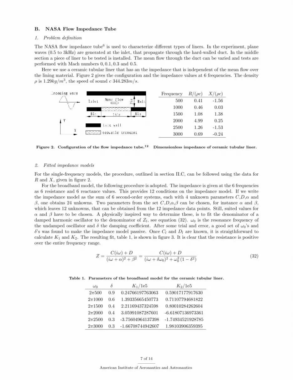
The NASA flow impedance tube6 is used to characterize different types of liners. In the experiment, planewaves (0.5 to 3kHz) are generated at the inlet, that propagate through the hard-walled duct. In the middlesection a piece of liner to be tested is installed. The mean flow through the duct can be varied and tests areperformed with Mach numbers 0, 0.1, 0.3 and 0.5.
Here we use a ceramic tubular liner that has an the impedance that is independent of the mean flow overthe lining material. Figure 2 gives the configuration and the impedance values at 6 frequencies. The densityρ is 1.29kg/m3, the speed of sound c 344.283m/s.
Frequency R/(ρc) X/(ρc)500 0.41 -1.56
1000 0.46 0.031500 1.08 1.382000 4.99 0.252500 1.26 -1.533000 0.69 -0.24
Figure 2. Configuration of the flow impedance tube.12 Dimensionless impedance of ceramic tubular liner.
2. Fitted impedance models
For the single-frequency models, the procedure, outlined in section II.C, can be followed using the data forR and X, given in figure 2.
For the broadband model, the following procedure is adopted. The impedance is given at the 6 frequenciesas 6 resistance and 6 reactance values. This provides 12 conditions on the impedance model. If we writethe impedance model as the sum of 6 second-order systems, each with 4 unknown parameters C,D,α andβ, one obtains 24 unkowns. Two parameters from the set C,D,α,β can be chosen, for instance α and β,which leaves 12 unknowns, that can be obtained from the 12 impedance data points. Still, suited values forα and β have to be chosen. A physically inspired way to determine these, is to fit the denominator of adamped harmonic oscillator to the denominator of Zl, see equation (32). ω0 is the resonance frequency ofthe undamped oscillator and δ the damping coefficient. After some trial and error, a good set of ω0’s andδ’s was found to make the impedance model passive. Once Cl and Dl are known, it is straigthforward tocalculate K1 and K2. The resulting fit, table 1, is shown in figure 3. It is clear that the resistance is positiveover the entire frequency range.
Z =C(iω) +D
(iω + α)2 + β2=
C(iω) +D
(iω + δω0)2 + ω20 (1− δ2)
(32)
Table 1. Parameters of the broadband model for the ceramic tubular liner.
ω0 δ K1/1e5 K2/1e52π500 0.9 0.24766197763063 0.590171779176302π1000 0.6 1.39335665450773 0.711077946818222π1500 0.4 2.21169437324598 0.800102842626042π2000 0.4 3.05991087287601 -6.618071369733612π2500 0.3 -3.75604964137398 -1.749345219287852π3000 0.3 -1.66708744942607 1.98103906359395
7 of 14
American Institute of Aeronautics and Astronautics

Figure 3. Real and imaginary part of fitted broadband impedance model.
3. Results
The duct is discretized by square elements of order 2 with a size of 1 inch. This leads to a very coarsemesh, for the domain only 32 × 2 elements are used, At the inlet and outlet the Perfectly Matched Layerformulation16 is used. The timestep is chosen as 4 · 10−6 seconds, the end time as 0.01 seconds.
The mean flow is modelled as a shear flow. The chosen shape is a parabole with maximum value equalto the Mach numbers given in the problem definition. As it is equal to zero at the walls, no modificationsare needed to the impedance condition: the same formulation as in the no-flow case applies. Previousresearch12,13 indicated the shear mean flow description to be superior to the effective plane-wave impedancecondition of Ingard14 and the convection-modified impedance condition of Myers.15 It was found to be moregeneral and stable.
For a single frequency simulation, a wave in the direction of the duct is imposed. For a broadbandsimulation, a sum of waves, one for each of the 6 frequencies, is imposed with a phase difference of π/6between each successive wave, as was done in reference.3 To compare the results, a Fast Fourier Transformis computed of the recorded pressure signal.
Figure 4 shows the results for the no-flow case. In general, the agreement is excellent, the amplitudes inthe single frequency simulation (+ signs) are almost everywhere identical to the amplitudes in the broadbandsimulation (solid line) for the same frequency. They are both very close to reference data. Only at 500Hzthe amplitudes are overestimated and differ a little. Other formulations12,13 have reached similar results forthe lowest frequency.
Figure 5 shows the results for a mean flow with Mach number 0.1. The three curves are virtually identicalfor each frequency and perfect agreement of the simulations and the experiment can be concluded.
Figure 6 shows the results for a mean flow with Mach number 0.3. The same conclusion can be reached asfor the case with Mach number 0.1: the numerical results are in very good agreement with the experimentalreference values. The curve of the single frequency simulation at 500Hz is missing as it showed oscillationsnear the inflow region. These are probably due to some instability in the Perfectly Matched Layer. Thebroadband simulation also shows some similar behaviour, albeit less severe.
Figure 7 shows the results for a mean flow with Mach number 0.5. The numerical results are still goodfor the middle frequencies, but the limitations of the assumed parabolic mean flow profile start to show.The predictions are none the less able to give a indication of the noise reduction. Also here the curve of thesingle frequency simulation for 500Hz is missing because of same reason as explained for the 0.3 case.
IV. Conclusions
To be physically feasible, a time-domain formulation has to comply with 3 necessary conditions. It hasto be causal, real and passive. The proposed general impedance/admittance model is causal and real. Aproper selection of parameters makes it also passive. Specifically for single-frequency simulations, a modelis proposed that can be matched to any given impedance at any given frequency.
The formulation is suited for broadband simulations by inclusion of multiple poles. An efficient imple-
8 of 14
American Institute of Aeronautics and Astronautics

Figure 4. Sound Pressure Level along upper wall for Mach number 0 (−: multifrequency simulation, +: singlefrequency simulation, o: reference data from measurements
9 of 14
American Institute of Aeronautics and Astronautics

Figure 5. Sound Pressure Level along upper wall for Mach number 0.1 (−: multifrequency simulation, +: singlefrequency simulation, o: reference data from measurements
10 of 14
American Institute of Aeronautics and Astronautics
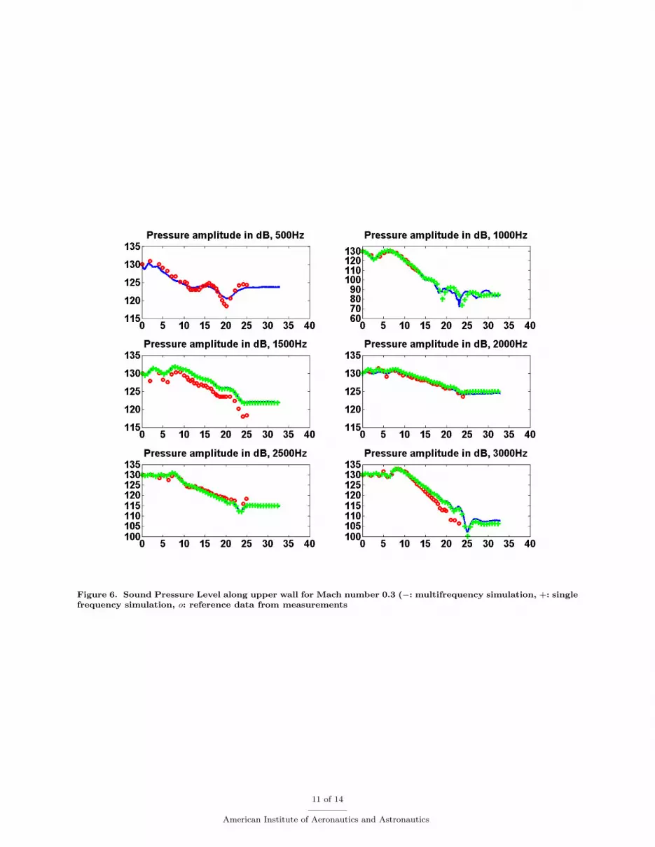
Figure 6. Sound Pressure Level along upper wall for Mach number 0.3 (−: multifrequency simulation, +: singlefrequency simulation, o: reference data from measurements
11 of 14
American Institute of Aeronautics and Astronautics

Figure 7. Sound Pressure Level along upper wall for Mach number 0.5 (−: multifrequency simulation, +: singlefrequency simulation, o: reference data from measurements
12 of 14
American Institute of Aeronautics and Astronautics

mentation is obtained by performing recursive convolution. This technique requires only some additions andmultiplications. The storage is limited to (complex-valued) accumulators in the boundary points. No timehistory of solution data is required, neither is there a need to compute time derivatives.
The single frequency and broadband formulations have been successfully validated for the NASA Langleyflow tube benchmark, with and without mean flow, for 6 frequencies. The use of a shear flow description ofthe mean flow proves to be an adequate choice.
Acknowledgments
The research of Yves Reymen is supported by a fellowship of the Institute for the Promotion of Innovationthrough Science and Technology in Flanders (IWT-Vlaanderen).
References
1Rienstra, S. W., “Impedance models in time domain”, Messiaen - Project AST3-CT-2003-502938, Deliverable 3.5.1 ofTask 3.5.
2Tam, CKW, Auriault, L., “Time-Domain Impedance Boundary Conditions for Computational Aeroacoustics”, AIAAJournal, Vol. 34, No. 5, 1996, pp. 917-923.
3Ozyoruk, Y., Long, L.N., Jones, M.G., “Time-Domain Numerical Simulation of a Flow-Impedance Tube”, Journal ofComputational Physics, Vol. 146, 1998, pp. 29-57.
4Fung, K.-Y., Ju, H., “Broadband Time-Domain Impedance Models”, AIAA Journal, Vol. 39, No. 8, 2001, pp. 1449-1454.5Keefe, L. R., Reisenthel, P. H., “Time-Domain Characterization of Acoustic Liner Response from Experimental Data
Part1: Linear Response”, 11th AIAA/CEAS Aeroacoustics Conference, AIAA paper 2005-3060.6Parrott, T.L., Watson, W.R., Jones, M.G., “Experimental Validation of a Two-Dimensional Shear-Flow Model for De-
termining Acoustic Impedance”, NASA TP-2679, May 1987.7Luebbers, R. J., “FDTD for Nth order Dispersive Media”, IEEE Transactions on antennas and propagation, Vol. 40,
No. 11, 1992, pp. 1297-1301.8Kelley, D. F., Luebbers, R. J., “Piecewise Linear Recursive Convolution for Dispersive Media using FDTD”, IEEE
Transactions on antennas and propagation, Vol. 44, No. 6, 1996, pp. 792-797.9Reymen, Y., et al., “A 3D Discontinuous Galerkin Method for Aeroacoustic Propagation”, Twelfth International Congress
on Sound and Vibration, 2005, paper 387.10Botteldooren, D., “Finite-diference time-domain simulation of low-frequency room acoustic problems”. Journal of the
Acoustical Society of America, Vol. 98, No. 6, 1995.11Zheng, S., Zhuang, M., “A Computational Aeroacoustics Prediction Tool for Duct Acoustics with Analytical and Exper-
imental Validations”, 9th AIAA/CEAS Aeroacoustics Conference, AIAA paper 2003-3248.12Li, X. L., Thiele, F., “Numerical Computation of Sound Propagation in Lined Ducts by Time-Domain Impedance
Boundary Conditions”, 10th AIAA/CEAS Aeroacoustics Conference, AIAA paper 2004-2902.13Ju, H., Fung, K.-Y., “Time-Domain Impedance Boundary Conditions with Mean Flow Effects”, Vol. 39, No. 9, 2001, pp.
1683-1690.14Ingard, U., “Influence of Fluid Motion Past a Plane Boundary on Sound Reflection, Absorption and Transmission”,
Journal of the Acoustical Society of America, Vol. 31, No. 7, 1959, pp. 1035-1036.15Myers, M. K., “On the Acoustic Boundary Condition in the Presence of Flow”, Journal of Sound and Vibration, Vol. 71,
No. 3. 1980. pp. 429-434.16Hu, F. Q., “Absorbing Boundary Conditions”, International Journal of Computational Fluid Dynamics, Vol. 18, No. 6,
2004, pp. 513-522.17Carpenter, M.H., Kennedy, C.A., “A fourth-order 2N-storage Runge-Kutta scheme”, NASA TM 109112, June, 1994.
Appendix
A proof for the recursive updating starts from the definition of the accumulator and proceeds withsplitting of the term containing the velocity of the last time step. The subsequent algebraic manipulationswrite the remaining sum as the definition of the accumulator at the previous time step. The most important
13 of 14
American Institute of Aeronautics and Astronautics

relationship used is χm+1k = e−λk∆tχm
k and likewise for ξk.
ψk(n∆t) =n−1∑m=0
(vn−m
n χmk + (vn−m−1
n − vn−mn )ξm
k
)(33)
=(vn
nχ0k + (vn−1
n − vnn)ξ0k
)+
n−1∑m=1
(vn−m
n χmk + (vn−m−1
n − vn−mn )ξm
k
)(34)
=(vn
nχ0k + (vn−1
n − vnn)ξ0k
)+
n−2∑m=0
(v(n−1)−m
n χm+1k + (v(n−1)−m−1
n − v(n−1)−mn )ξm+1
k
)(35)
=(vn
nχ0k + (vn−1
n − vnn)ξ0k
)+ e−λk∆t
n−2∑m=0
(v(n−1)−m
n χmk + (v(n−1)−m−1
n − v(n−1)−mn )ξm
k
)(36)
=(vn
nχ0k + (vn−1
n − vnn)ξ0k
)+ e−λk∆tψk((n− 1)∆t) (37)
The proof for ψ̂l follows exactly the same steps, using the relationship χ̂m+1 = e(−αl+iβl)∆tχ̂m and likewisefor ξ̂l.
χ0k, ξ
0k, χ̂
0l and ξ̂0l have been replaced in the formulation (22-24), through the definitions (19-20), with
expressions in terms of the poles λk, −α+ iβ and the timestep ∆t.
14 of 14
American Institute of Aeronautics and Astronautics