Pac-Learning Non-Recursive Prolog ClausesWilliam W. CohenAT&T Bell Laboratories600 Mountain Avenue Murray Hill, NJ 07974(908)-582-2092wcohen@research.att.comMay 31, 1995AbstractRecently there has been an increasing amount of research on learning concepts ex-pressed in subsets of Prolog; the term inductive logic programming (ILP) has beenused to describe this growing body of research. This paper seeks to expand the theo-retical foundations of ILP by investigating the pac-learnability of logic programs. Wefocus on programs consisting of a single function-free non-recursive clause, and focuson generalizations of a language known to be pac-learnable: namely, the language ofdeterminate function-free clauses of constant depth. We demonstrate that a number ofsyntactic generalizations of this language are hard to learn, but that the language canbe generalized to clauses of constant locality while still allowing pac-learnability. Morespeci�cally, we �rst show that determinate clauses of log depth are not pac-learnable,regardless of the language used to represent hypotheses. We then investigate the e�ectof allowing indeterminacy in a clause, and show that clauses with k indeterminate vari-ables are as hard to learn as DNF. We next show that a more restricted language ofclauses with bounded indeterminacy is learnable using k-CNF to represent hypotheses,and that restricting the \locality" of a clause to a constant allows pac-learnability evenif an arbitrary amount of indeterminacy is allowed. This last result is also shown tobe a strict generalization of the previous result for determinate function-free clauses ofconstant depth. Finally, we present some extensions of these results to logic programswith multiple clauses. To appear in Arti�cial Intelligence

1 IntroductionRecently there has been an increasing amount of research on learning concepts expressedin �rst-order logics. While some researchers have considered special-purpose logics such asdescription logics as a representation for concepts and examples [Vilain et al., 1990; Kietzand Morik, 1991; Cohen and Hirsh, 1992] most researchers have used standard �rst-orderlogic as a representation language; in particular, most have used restricted subsets of Prologto represent concepts [Cohen, 1992; Muggleton and Feng, 1992; Pazzani and Kibler, 1992;Quinlan, 1990; Muggleton, 1992c]. The term inductive logic programming (ILP) has beenused to describe this growing body of research.One advantage of basing learning systems on Prolog is that its semantics and complexityare mathematically well-understood. This o�ers some hope that learning systems based onit can also be rigorously analyzed. A number of formal results have in fact been obtained;in particular, a number of previous researchers have derived learnability results in Valiant's[1984] model of pac-learnability [Haussler, 1989; Frisch and Page, 1991; D�zeroski et al., 1992;Kietz, 1993]. This paper seeks to expand the theoretical foundations of ILP by furtherinvestigating the pac-learnability of logic programs. In particular, our goal is to investigatecarefully the degree to which the representational restrictions imposed by certain practicalsystems are necessary; in other words, we wish to determine the representational \boundariesof learnability" for logic programs, rather than to analyze existing learning systems.In this paper we will consider primarily logic programs consisting of a single function-free non-recursive clause. We focus on single clauses because the results that are obtainableon the learnability of multiple clause programs are straightforward extensions of results forsingle clauses [D�zeroski et al., 1992; Cohen, 1993c]. We consider only non-recursive clauseshere because analysis of recursive programs requires somewhat di�erent formal machinery[Cohen, 1993c; Cohen, 1993a]; we also note that recursion has not been important in severalapplications of ILP methods to real-world problems [Muggleton, 1992a; Feng, 1992; King etal., 1992; Muggleton et al., 1992]. A �nal restriction is that while background knowledge willbe allowed in our analysis, we will allow only background theories of ground unit clauses (akaa database or a model.) This restriction has also been made by several practical learningsystems [Quinlan, 1990; Pazzani and Kibler, 1992; Muggleton and Feng, 1992].In this paper, we will �rst de�ne pac-learnability and review previous learnability resultsfor logic programs: the most important of these (for the purpose of this paper) shows thata single determinate function-free clause of constant depth1 is pac-learnable [D�zeroski et al.,1992]. We then investigate a number of generalizations of this language, beginning withthe language of determinate clauses of logarithmic depth (rather than constant depth). Weshow that this language is not pac-learnable, regardless of the language used to representhypotheses.We then investigate the e�ect of allowing indeterminacy in a clause, and obtain a seriesof results for indeterminate clauses. We show that clauses with even a single \free" variableare as hard to learn as DNF, and that a slightly more restricted language of clauses with\bounded indeterminacy" is not pac-learnable, but is predictable, using k-CNF to representhypotheses. Both of these results are negative, as they demonstrate that apparently rea-1These restrictions are precisely de�ned in Section 2.5.1

sonable languages are surprisingly hard to learn. However, we next show that bounding the\locality" of a clause allows pac-learnability, even if an arbitrary amount of indeterminacyis allowed.Our last result on indeterminate clauses concerns the relative expressive power of ij-determinate clauses and clauses with bounded locality: we show that for �xed i and j,every ij-determinate clause can be rewritten as a clause with locality no greater than ji+1.Thus, the language of clauses of bounded locality is, in a very reasonable sense, a strictgeneralization of the language of ij-determinate clauses.To summarize these results, we show that although the obvious syntactic generalizationsof ij-determinacy all fail to produce pac-learnable languages, generalizing to the languageof clauses bounded locality does yield a pac-learnable language.Finally, we state some additional results on the learnability of multiple-clause nonrecur-sive programs, discuss related work, and conclude.A number of the results in this paper have been previously presented in a preliminary formelsewhere [Cohen, 1993a; Cohen, 1993b; Cohen, 1994a]. The pac-learnability of recursiveprograms, another interesting formal issue, is considered in depth in a companion paper[Cohen, 1994b].2 Preliminaries2.1 Logic programmingIn this section, we will give an overview of logic programming. As we are consideringvery simple logic programs, our overview has been simpli�ed accordingly; in particular, thede�nitions below only coincide with the usual ones for the case of non-recursive function-freesingle-clause Prolog programs. For a more complete description of logic programming thereader is referred to one of the standard texts (e.g., [Lloyd, 1987]).Logic programs are written over an alphabet of constant symbols, which we will usuallyrepresent with letters like t1; t2; : : :, an alphabet of predicate symbols, which we will usuallyrepresent with letters like p, q or r, and an alphabet of variables, which we will alwaysrepresent with upper case letters. A literal is written p(X1; : : : ;Xk) where p is a predicatesymbol and X1, : : : , Xk are variables. The number of arguments k in a literal is calledthe arity of the literal. A fact is written p(t1; : : : ; tk) where p is a predicate symbol andt1, : : : , tk are constant symbols; again, the arity of a fact is the number of arguments k.A substitution is a partial function mapping variables to constant symbols or variables; wewill represent substitutions with the Greek letters � and � and (when necessary) write themas sets � = fX1 = t1;X2 = t2; : : : ;Xn = tng where ti is the constant symbol onto whichXi is mapped. If � is a substitution and A is a literal, we will use A� to denote the resultof replacing each variable X in A with the constant symbol to which X is mapped by �;extending this notation slightly, if �1 and �2 are both substitutions, we will use A�1�2 todenote (A�1)�2.A fact f is an instance of a literal A if there is some substitution � such that A� = F . If�1 and �2 are substitutions such that �1 � �2, then we say that �1 is more general than �2.Notice that if �1 is more general than �2, then for any literal A, the set of instances of A�12

is a superset of the set of instances of A�2.Finally, a de�nite clause is written A B1 ^ : : :^Bl where A and B1; : : : ; Bl are literals.A is called the head of the clause, and the conjunction B1 ^ : : :^Bl is called the body of theclause. If DB is a set of facts|which we will also call a database|then the extension of aclause A B1 ^ : : : ^ Bl with respect to the database DB is the set of all facts f such thateither� f 2 DB, or� there exists a substitution � so that A� = f , and for every Bi from the body of theclause, Bi� 2 DB.In the latter case, we will say that the substitution � proves f to be in the extension of theclause. For brevity, we will let ext (C;DB) denote the extension of C with respect to thedatabase DB.For technical reasons, it will be convenient to assume that every database DB containsan equality predicate|that is, a predicate symbol equal such that equal (ti; ti) 2 DB for everyconstant ti appearing in DB, and equal (ti; tj) 62 DB for any ti 6= tj. This assumption can bemade without loss of generality, since such a predicate can be added to any database withonly a polynomial increase in size.Readers familiar with logic programming will notice that this de�nition of \extension"coincides with the usual �xpoint or minimal-model semantics of Prolog programs for the pro-grams considered in this paper (i.e., single clause function-free nonrecursive Prolog programsover a ground background theory). Hence one might more succinctly de�ne the extension ofa clause C with respect to DB as ff : C ^DB ` fg.Again for those familiar with �rst order logic, a clause A B1 ^ : : : ^ Bl can also bethought of as a logical statement8X1; : : : ;Xn (:B1 _ : : : _ :Bl _ A)where X1; : : : ;Xn are the variables that appear in the clause. Then the extension of a clausewith respect to DB is simply the set of facts e that follow from the logical statement aboveand the conjunction of the facts in DB.Example. If DB is the setDB = fmother(ann,bob),father(bob,julie),father(bob,chris)gthen the extension of the clausegrandmother(X,Y) mother(X,Z),father(Z,Y)with respect to DB is the setDB [ fgrandmother(ann,julie),grandmother(ann,chris)g3

(Notice that we have adopted the convention that a function f is representedby a predicate f(X;Y ) where f(X;Y ) is true i� Y = f(X).) The most generalsubstitutions that prove the additional factsf1 = grandmother(ann,julie)f2 = grandmother(ann,chris)are in the extension are�1 = fX = ann; Y = julie; Z = bobg�2 = fX = ann; Y = chris; Z = bobg2.2 Models of learnabilityOur goal is to determine by formal analysis which subsets of Prolog are e�ciently learnable;we focus in this paper on the case of function-free non-recursive Prolog. Any formal analysisof learnability, of course, requires an explicit model of what it means for a language to be\e�ciently learnable." In this section, we will describe our basic models of learnability; theseare slight modi�cations of the models of pac-learnability, introduced by Valiant [1984], andpolynomial predictability, introduced by Pitt and Warmuth [1990].Let X be a set, called the domain. De�ne a concept C over X to be a representationof some subset of X, and a language Lang to be a set of concepts. Associated with Xand Lang are two size complexity measures. We will write the size complexity of someconcept C 2 Lang or instance e 2 X as jjCjj or jjejj, and we will assume that this measure ispolynomially related to the number of bits needed to represent C or e. We use the notationXn (respectively Langn) to stand for the set of all elements of X (respectively Lang) of sizecomplexity no greater than n. In this paper, we will be rather casual about the distinctionbetween a concept and the set it represents; when there is a risk of confusion we will referto the set represented by a concept C as the extension of C.Example. For example, let X be the domain of binary vectors, interpretedas assignments to boolean variables, and let Dnf be the language of booleanformulae in disjunctive normal form. One might measure the complexity of avector e 2 X as the length of the vector, and measure the complexity of aformula C by the number of literals in C. Thus for the instance e = 00110 wehave jjejj = 5, and for the concept C = ((x1 ^ x5) _ (x1 ^ x5)) we have jjCjj = 4.An example of C is a pair (e; b) where b = 1 if e 2 C and b = 0 otherwise. If D is aprobability distribution function, a sample of C from X drawn according to D is a pair ofmultisets S+; S� drawn from the domain X according to D, S+ containing only positiveexamples of C, and S� containing only negative ones. We can now de�ne our basic learningmodels.De�nition 1 (Polynomially predictable) A language Lang is polynomially predictablei� there is an algorithm PacPredict and a polynomial function m(1� ; 1� ; ne; nt) so that forevery nt > 0, every ne > 0, every C 2 Langnt , every � : 0 < � < 1, every � : 0 < � < 1, andevery probability distribution function D, PacPredict has the following behavior:4

1. given a sample S+; S� of C from Xne drawn according to D and containing at leastm(1� ; 1� ; ne; nt) examples, PacPredict outputs a hypothesis H such thatProb(D(H � C) +D(C �H) > �) < �where the probability is taken over the possible samples S+ and S� and (if PacPredictis a randomized algorithm) over any coin ips made by PacPredict;2. PacPredict runs in time polynomial in 1� , 1� , ne, nt, and the number of examples;and3. H can be evaluated in polynomial time.The algorithm PacPredict is called a prediction algorithm for Lang, and the functionm(1� ; 1� ; ne; nt) is called the sample complexity of PacPredict.We will sometimes abbreviate \polynomial predictability" as \predictability".The �rst condition in the de�nition merely states that the error of the hypothesis must(usually) be low, as measured against the probability distribution D from which the trainingexamples were drawn. The second condition, together with the stipulation that the samplesize is polynomial, ensures that the total running time of the learner is polynomial. The �nalcondition simply requires that the hypothesis be usable in the very weak sense that it canbe used to make predictions in polynomial time. Notice that this is a worst case learningmodel, as the de�nition allows an adversarial choice of all the inputs of the learner.The model of polynomial predictability has been well-studied [Pitt and Warmuth, 1990],and is a weaker version of Valiant's [1984] criterion of pac-learnability:De�nition 2 (Pac-learnable) A language Lang is pac-learnable i� there is an algorithmPacLearn so that1. PacLearn satis�es all the requirements in the de�nition of polynomial predictability,and2. on inputs S+ and S�, PacLearn always outputs a hypothesis H 2 Lang.Thus if a language is pac-learnable it is predictable, but the converse need not be true.Predictability also has an important property not shared by pac-learnability: if a languageis not predictable, then no superset of that language is predictable. In other words, onecannot make a non-predictable language predictable by generalizing the language, only byadding additional restrictions. Showing a language is not predictable indicates that thelanguage is, in some sense, too expressive to learn e�ciently, and hence is a strong negativeresult.On the other hand, in ILP contexts, it is often considered desirable to output hypothesesthat are logic programs; hence a polynomial prediction algorithm, which may output hy-potheses in an arbitrary format, may be much less desirable than a pac-learning algorithm.Thus ideally one would like all positive results to be given in the pac-learning model, andall negative results to be given in the polynomial prediction model. In this paper we will(whenever possible) give positive results in the pac-learning model, and use predictabilityprimarily in negative results. 5

2.3 Background knowledge: extending the standard modelsSo far, our formalization is standard. However, in a typical ILP system, the user providesboth a set of examples and a \background theory" de�ning a set of predicates that may beuseful in constructing a hypothesis: the task of the learner is then to �nd a logic program Psuch that P , together with the background theory, is a good model of the data.To account for the background knowledge, it is necessary to extend the model of learn-ability. One way of doing this is to allow examples to be clauses that are entailed by thetarget concept [Plotkin, 1969; Shapiro, 1982; Frazier and Pitt, 1993]. However, in this paper,we will follow Haussler [1989] and D�zeroski et al. in using a closely related formalism whichmore directly models the typical use of background knowledge in ILP systems.If Lang is some set of de�nite clauses and DB is a database, then Lang[DB] denotesthe set of pairs of the form (C;DB) such that C 2 Lang. Each such pair represents theextension of C with respect to DB, as de�ned in Section 2.1|i.e., the set of all facts e suchthat C ^ DB ` e. If DB is some set of databases, then Lang[DB] denotes the set of alllanguages Lang[DB] where DB 2 DB. Such a set of languages will be called a languagefamily. The set of de�nite clauses Lang will be called a clause language.In this paper, we will consider primarily the learnability of language families, usinglearning algorithms that accept a database as input in addition to the usual set of trainingexamples. The following de�nitions extend the notions of pac-learnability and polynomialpredictability to this new setting.De�nition 3 A language family Lang[DB] is polynomially predictable i� for every DB 2DB there is a prediction algorithm PacPredictDB for Lang[DB].A language family Lang[DB] is uniformly polynomially predictable i� it is polynomiallypredictable and there is a algorithm PacPredict(DB; S+; S�), which runs in time polyno-mial in all of its inputs, such that PacPredict, with its �rst argument �xed to be DB, is aprediction algorithm for LangDB.The (uniform) pac-learnability of a language family is de�ned analogously.Intuitively, a language family is predictable if it can be predicted regardless of thedatabase DB, and a language family is uniformly predictable if there is a single predictionalgorithm that works for all databases.Notice that PacPredict(DB; S+; S�) must run in time polynomial in all of its inputs,including the size of the database DB. Thus uniform predictability (and pac-learnability)requires the prediction (or learning) algorithm to scale well with the size of the backgrounddatabase DB.Finally, let us de�ne a-DB to be the set of databases containing only facts of arity a orless. Most of the results in this paper will be in one of the following forms:� For any �xed constant a, Lang[a-DB] is uniformly pac-learnable.Such a result means that even if one allows an adversary choice of the database DB,clauses in Lang[DB] are pac-learnable, that there is a known learning algorithm thatworks for any database DB, and furthermore that the algorithm requires time onlypolynomial in the size of the database DB. (However, it may require time exponential6

in the maximum arity a of facts in the database.) This is a strong positive result aboutthe learnability of clauses in Lang.� For every a � a0 (where a0 is some small �xed constant, say a0 = 3) Lang[a-DB] isnot predictable.Such a result means that for at least some databases DB 2 a-DB, clauses in Lang[DB]are not predictable (and hence not pac-learnable regardless of the representation usedfor hypotheses). This is a negative result about the learnability of clauses in Lang.The notions of uniform pac-learnability and predictability extend the standard modelsto the ILP setting, where the database is an additional input to the learner. The standardmodels are worst-case over all distributions and all target concepts; we have simply made thelearning model worst-case also over all possible choices of a database. At �rst glance, it mayseem odd to allow an adversarial choice of the database. This is reasonable, however, becauseif the database DB is such that the target concept cannot be expressed using predicatesde�ned in DB, or is only expressible by an extremely large concept, then the learning systemis not required to �nd an accurate hypothesis quickly (since time and sample complexitymay grow with the the size of the target concept C 2 Lang[DB]). Thus the model isactually worst-case over all databases DB that are \appropriate" in the sense that a conciserepresentation of the target concept can be found using the predicates de�ned in DB.We will typically use nb to denote the size of a database DB. The parameters ne, nt andnb all measure, in some sense, the size of the learning problem, and we are requiring thelearner to be polynomial in all of these size measures; while there is some value in keepingthese di�erent measures separate, the casual reader may �nd it easier to consider the resultsin terms of a single size measure n = ne + nb + nt.Example. As an example of an ILP learning problem, to learn the predicatematernal grandmother, the user might provide the databaseDB = f father(charlie,william), mother(charlie,susan),father(susan,dan), mother(susan,ruth),father(william,maurice), mother(william,caroline),father(rachel,maurice), mother(rachel,caroline),father(elizabeth,warren), mother(elizabeth,rachel) gand the examplesS+ = f maternal grandmother(charlie,ruth), maternal grandmother(elizabeth,caroline) gS� = f maternal grandmother(charlie,dan), maternal grandmother(william,caroline),maternal grandmother(ruth,dan), maternal grandmother(maurice,susan) gIn this problem, the user's database DB is in 2-DB, the size of the database isnb = 10, and the size of the examples is ne = 2. An ILP learning system for theclause language 1-DepthDeterm (see below for de�nition) might produce thehypothesis 7

H = maternal grandmother(X,Y) mother(X,Z) ^ mother(Z,Y).If the learning system were a pac-learning system with a known sample complex-ity, then (if S+ and S� were su�ciently large, and drawn from a �xed distribu-tion) one could make some guarantees about the error rate � of the learner. Note,however, that the user provides only the inputs S+, S�, and the database DB.2.4 Sample complexity of learning logic programsIn typical ILP problems the examples will all have the same predicate symbol p and arityne; thus, in e�ect, the predicate and arity of the head of the target clause are given. Oneimportant fact to note is the following.Theorem 4 Let Datalogp=ne be the language of all function-free nonrecursive clauses thathave a head with predicate symbol p and arity ne. Then for any �xed constant a and any DB 2a-DB, the Vapnik-Chervonenkis dimension [Blumer et al., 1989] of Datalogp=maxint [DB] ispolynomial in ne, nt and nb (where nb is the size of DB).Proof: We will establish an upper bound on the number of semantically di�erent clauses.A Datalog clause of size nt can contain at most ne + ant distinct variables, as at most nevariables can appear in the head, and at most ant variables can appear in the body; thusthere are at most (ne + ant)ne possible clause heads. Since there are at most nb predicatesthat appear in the database, and each literal consists of one such predicate symbol and aor fewer variables, there are at most nb(ne + ant)a literals that can appear in the body ofa clause that succeeds with the database DB. Putting these two bounds together, the totalnumber of semantically di�erent clauses is(ne + ant)ne � (nb(ne + ant)a)ntThe VC dimension is bounded by the logarithm of this quantityne log2 (ne + ant) + nt log2 (nb(ne + ant)a)which is polynomial in nb, ne, and nt.Blumer et. al [1989] show that if a concept class has polynomial VC dimension, then for acertain polynomial sample size, any consistent hypothesis H of minimal or near-minimal sizewill with high con�dence have low error. More speci�cally, any algorithm A that outputsa consistent hypothesis that is within a polynomial of the size of the smallest consistenthypothesis will satisfy all the requirements of pac-learning|except, perhaps, the requirementthat the learner run in polynomial time.Thus, the following simple procedure will satisfy all of the requirements of uniform pac-learnability for Datalog, except the requirement that the learning program be polynomial-time: enumerate all non-vacuous Datalog clauses in increasing order of size, and return the�rst clause that is consistent with the sample. Since this paper considers only languages thatare restrictions of Datalog, this means that if computational complexity is ignored, all ofthe languages considered in this paper are pac-learnable. The central question we address,then, is when polynomial-time learning is possible.8

2.5 Constant-depth determinacy and previous resultsMuggleton and Feng [1992] have introduced several useful restrictions on de�nite clauses,which we will now describe. If A B1 ^ : : : ^ Br is an (ordered) de�nite clause, then theinput variables of the literal Bi are those variables appearing in Bi that also appear in theclause A B1 ^ : : : ^Bi�1; all other variables appearing in Bi are called output variables. Aliteral Bi is determinate (with respect to DB) if for every possible substitution � that uni�esA with some fact e such that B1� 2 DB, B2� 2 DB, : : : , Bi�1� 2 DB there is at mostone substitution � so that Bi�� 2 DB. Less formally, a literal is determinate if its outputvariables have only one possible binding, given DB and the binding of the input variables.A clause is determinate if all of its literals are determinate. Informally, determinateclauses are those that can be evaluated without backtracking by a Prolog interpreter.Next, de�ne the depth of a variable appearing in a clause A B1 ^ : : : ^ Br as follows.Variables appearing in the head of a clause have depth zero. Otherwise, let Bi be the �rstliteral containing the variable V , and let d be the maximal depth of the input variables ofBi; then the depth of V is d+1. The depth of a clause is the maximal depth of any variablein the clause.Example. The clausematernal grandmother(C,G) mother(C,M) ^ mother(M,G)is determinate (assuming successor is functional). The maximum depth of avariable is one, for the variableM, and hence the clause has depth one. Assumingthat the predicates enclosed paper and length are determinate, the clauseunwelcome mail(E) envelope(E) ^enclosed paper(E,P) ^ must review(P) ^length(P,L) ^ gt50(L).is determinate and of depth two. The variable P from this clause has depth one,and the variable L has depth two.An interesting class of logic programs is the following.De�nition 5 (ij-determinate) A determinate clause of depth bounded by a constant iover a database DB 2 j-DB is called ij-determinate.The learning program GOLEM, which has been applied to a number of practical problems[Muggleton and Feng, 1992; Muggleton, 1992b], learns ij-determinate programs. Closelyrelated restrictions also have been adopted by several other inductive logic programmingsystems, including FOIL [Quinlan, 1991] and LINUS [Lavra�c and D�zeroski, 1992].The learnability of non-recursive ij-determinate clauses has also been formally studied[D�zeroski et al., 1992]. For notation, let i-DepthDeterm be the language of determinateclauses of depth i or less; the language family of ij-determinate clauses is thus denotedi-DepthDeterm[j-DB]. One important result is the following.9

Theorem 6 (D�zeroski, Muggleton & Russell) For any �xed i and j, the language fam-ily i-DepthDeterm[j-DB] is uniformly pac-learnable.Other previous work has established that a single clause is not pac-learnable if the ij-determinacy condition does not hold; speci�cally, it has been shown that neither the languageof indeterminate clauses of �xed depth nor the language of determinate clauses of arbitrarydepth is pac-learnable [Kietz, 1993]. The proof of these facts is based on showing that thereare sets of examples such that �nding a single clause in the language consistent with theexamples is NP-hard (or worse).Unfortunately, these negative results are of limited practical importance, because theyonly show learning to be hard when the learner is required to output a single clause consistentwith all of the examples. Most ILP learning systems, however, learn a set of clauses, not asingle clause, and the results do not show that learning using this more expressive represen-tation is intractable. Such negative learnability results are sometimes called representation-dependent .2 One of the goals of this paper is to develop representation-independent learningresults that complement the positive result of Theorem 6. These results will be developedshortly; �rst, however we will describe the analytic tool used to obtain the results.2.6 Reducibility among prediction problemsPitt and Warmuth [1990] have introduced a notion of reducibility between prediction prob-lems, analogous to the notion of reducibility for decision problems that is commonly usedto prove a problem NP-hard. Prediction-preserving reducibility is essentially a method ofshowing that one language is no harder to predict than another.De�nition 7 (Prediction-preserving reducibility) Let Lang1 be a language over do-main X1 and Lang2 be a language over domain X2. We say that predicting Lang1 reducesto predicting Lang2, denoted Lang1 � Lang2, if there is a function fi : X1 ! X2, hence-forth called the instance mapping, and a function fc : Lang1 ! Lang2, henceforth calledthe concept mapping, so that the following all hold:1. x 2 C if and only if fi(x) 2 fc(C) | i.e., concept membership is preserved by themappings;2. the size complexity of fc(C) is polynomial in the size complexity of C | i.e. the sizeof concept representations is preserved within a polynomial factor;3. fi(x) can be computed in polynomial time.Note that fc need not be computable; also, since fi can be computed in polynomial time,fi(x) must also preserve size within a polynomial factor.2The prototypical example of a learning problem that is hard in a representation-dependent setting butnot in a broader setting is learning k-term DNF. Assuming that RP 6= NP , pac-learning k-term DNF isintractable if the hypotheses of the learning system must be k-term DNF, but tractable if hypotheses canbe expressed in the richer language of k-CNF [Pitt and Valiant, 1988].10

Intuitively, fc(C1) returns a concept C2 2 Lang2 that will \emulate" C1|i.e., make thesame decisions about concept membership|on examples that have been \preprocessed" withthe function fi. If predicting Lang1 reduces to predicting Lang2 and a learning algorithmfor Lang2 exists, then one possible scheme for learning concepts from Lang1 would be thefollowing. First, convert any examples of the unknown concept C1 from the domain X1to examples over the domain X2 using the instance mapping fi. If the conditions of thede�nition hold, then since C1 is consistent with the original examples, the concept fc(C1)will be consistent with their image under fi; thus running the learning algorithm for Lang2should produce some hypothesis H that is a good approximation of fc(C1). Of course, itmay not be possible to map H back into the original language Lang1, as computing fc�1may be di�cult or impossible. However, H can still be used to predict membership in C1:given an example x from the original domain X1, one can simply predict x 2 C1 to be truewhenever fi(x) 2 H.Pitt and Warmuth [1988] give a more rigorous argument that this approach leads to aprediction algorithm for Lang1, leading to the following theorem.Theorem 8 (Pitt and Warmuth) Assume that Lang1 � Lang2. Then the followinghold:� If Lang2 is polynomially predictable, then Lang1 is polynomially predictable.� If Lang1 is not polynomially predictable, then Lang2 is not polynomially predictable.The second case of the theorem allows one to transfer hardness results from one languageto another; this is useful because for a number of languages, it is known that prediction isas hard as breaking cryptographic schemes that are widely assumed to be secure. The �rstcase of the theorem gives a means of obtaining a prediction algorithm for Lang1, given aprediction algorithm for Lang2.If fc is one-to-one and fc�1 is computable, then the reduction is said to \invertible"; inthis case it can be shown that if Lang2 is pac-learnable then Lang1 is also pac-learnable.For example, the proof of Theorem 6 is based on an invertible prediction-preserving reductionbetween ij-determinate clauses and monotone monomials.3 Log-depth clauses are hard to learnIn the next two sections, we will investigate the learnability of de�nite clauses in the modelsdescribed above: pac-learnability and polynomial predictability. Our starting point will beTheorem 6|in particular, we will consider generalizing the result of Theorem 6 by gen-eralizing the de�nition of ij-determinacy in various ways, and seeing if the correspondinglanguages are learnable.We will �rst consider relaxing the restriction that clauses have constant depth. Muggletonand Feng [1992] argue that many practically useful programs are limited in depth; however,in the list of clauses they provide as examples to support their argument, it is frequently thecase that the more complex clauses have greater depth. It might be plausibly argued that it11

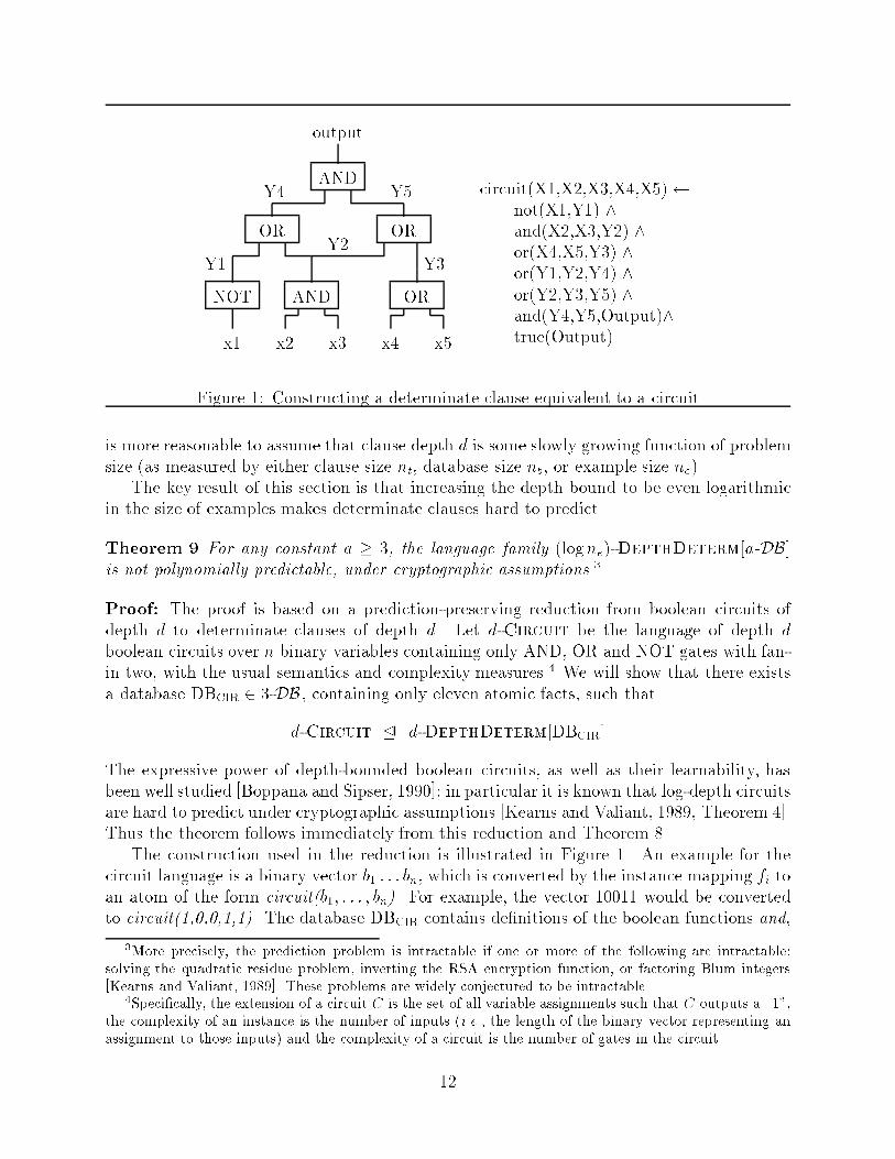
Y2Y4Y1 Y5 Y3outputx5x4x3x2x1NOT AND OROR ORAND circuit(X1,X2,X3,X4,X5) not(X1,Y1) ^and(X2,X3,Y2) ^or(X4,X5,Y3) ^or(Y1,Y2,Y4) ^or(Y2,Y3,Y5) ^and(Y4,Y5,Output)^true(Output)Figure 1: Constructing a determinate clause equivalent to a circuitis more reasonable to assume that clause depth d is some slowly growing function of problemsize (as measured by either clause size nt, database size nb, or example size ne).The key result of this section is that increasing the depth bound to be even logarithmicin the size of examples makes determinate clauses hard to predict.Theorem 9 For any constant a � 3, the language family (log ne)-DepthDeterm[a-DB]is not polynomially predictable, under cryptographic assumptions.3Proof: The proof is based on a prediction-preserving reduction from boolean circuits ofdepth d to determinate clauses of depth d. Let d-Circuit be the language of depth dboolean circuits over n binary variables containing only AND, OR and NOT gates with fan-in two, with the usual semantics and complexity measures.4 We will show that there existsa database DBCIR 2 3-DB, containing only eleven atomic facts, such thatd-Circuit � d-DepthDeterm[DBCIR]The expressive power of depth-bounded boolean circuits, as well as their learnability, hasbeen well studied [Boppana and Sipser, 1990]; in particular it is known that log-depth circuitsare hard to predict under cryptographic assumptions [Kearns and Valiant, 1989, Theorem 4].Thus the theorem follows immediately from this reduction and Theorem 8.The construction used in the reduction is illustrated in Figure 1. An example for thecircuit language is a binary vector b1 : : : bn, which is converted by the instance mapping fi toan atom of the form circuit(b1; : : : ; bn). For example, the vector 10011 would be convertedto circuit(1,0,0,1,1). The database DBCIR contains de�nitions of the boolean functions and,3More precisely, the prediction problem is intractable if one or more of the following are intractable:solving the quadratic residue problem, inverting the RSA encryption function, or factoring Blum integers[Kearns and Valiant, 1989]. These problems are widely conjectured to be intractable.4Speci�cally, the extension of a circuit C is the set of all variable assignments such that C outputs a \1",the complexity of an instance is the number of inputs (i.e., the length of the binary vector representing anassignment to those inputs) and the complexity of a circuit is the number of gates in the circuit.12

or, and not, as well as a de�nition of the unary predicate true, which succeeds whenever itsargument is a \1":DBCIR = f and(0,0,0), and(0,1,0), or(0,0,0), or(0,1,1), not(0,1),and(1,0,0), and(1,1,1), or(1,0,0), or(1,1,1), not(1,0), true(1) gFinally, the concept mapping fc is as indicated in the �gure. To be precise, for each gateGi in the circuit there is a single literal Li with a single output variable Yi, de�ned asLi � 8><>: and(Zi1; Zi2; Yi) if Gi is an AND gateor(Zi1; Zi2; Yi) if Gi is an OR gatenot(Zi1; Yi) if Gi is an NOT gatewhere in each case the Zij's are the variables that correspond to the input(s) to Gi. Assumewithout loss of generality that the numbering for the Gi's always puts all the inputs to agate Gj before Gj in the ordering; then the clause fc(C) is simplyfc(C) � circuit(X1; : : : ;Xn) ( ni=1Li) ^ true(Yn)Notice that the construction preserves depth.The algorithm presented by Muggleton and Feng for learning a single ij-determinateclause is doubly exponential in the depth of the clause. The result above shows that nolearning algorithm for determinate clauses exists that improves this bound much, e.g., thatis even singly exponential in depth. The result holds even for learning systems that use analternative representation for their hypotheses (e.g., systems that approximate one clausewith several.)Recent work has shown that log-depth circuits are hard to predict even if examples aredrawn from a uniform distribution [Kharitonov, 1992].5 Thus even making fairly strongassumptions about the distribution of examples will not make log-depth determinate clausespredictable.4 Hard-to-learn indeterminate clausesThe results of Section 3 indicate that one is not likely to be able to generalize the classof ij-determinate clauses by increasing the depth bound. We will now consider relaxingthe second key aspect of the ij-determinacy restriction: the condition that clauses be de-terminate. While for many problems determinacy is an appropriate restriction, there arereal-world problems for which some of the background knowledge cannot be accessed usingonly determinate literals [Cohen, 1993d]; thus for practical reasons, it would be useful to beable to relax this restriction.In this section, we will consider several plausible ways to relax the determinacy restriction,and show that these relaxations lead to languages that are hard to pac-learn and (in most5This case requires the additional cryptographic assumption that solving the n�n1+� subset sum is hard.13

cases) also hard to predict. In particular, we �rst consider bounding the depth of a clause,but not restricting it in any other way, and show that this leads to a language that is hardto predict. We then consider bounding the number of \free" variables in an indeterminateclause, and show that this language is exactly as hard to predict as DNF. We then consideran alternative set of restrictions in which the degree of indeterminacy is also bounded, andshow that that language is predictable, but not pac-learnable.4.1 Constant-depth indeterminate clausesThe most obvious way of relaxing ij-determinacy would be to consider constant-depth clausesthat are not determinate. Unfortunately, this leads to a language family that is hard to learn.Letting k-Depth denote the language of all clauses of depth k or less, we have the followingresult:Theorem 10 For a � 3 and k � 1, the language family k-Depth[a-DB] is not predictable,unless NP � P=Poly.Proof: Schapire [1990] shows that if a language Lang is polynomially predictable, thenevery C 2 Lang can be emulated by a polynomial-sized circuit. To prove the theorem,therefore, it is su�cient to construct a polynomial sized database DB 2 3-DB such that forsome C 2 1-Depth[DB] testing membership in C is NP-hard.Let DB contain the following predicates:� The predicate boolean(X) is true if X = 0 or X = 1.� For k = 1 through n, the predicate linkk(M,V,X) is true if M 2 f�n; : : : ;�1g orM 2 f1; : : : ; ng, V 2 f0; 1g, X 2 f0; 1g, and one of the following conditions also holds:{ M = k and X = V{ M = �k and X = :V{ M 6= k and M 6= �k (and X and V have any values).� Finally, the predicate sat(V1; V2; V3) is true if each Vi 2 f0; 1g and if one of V1; V2; V3 isequal to 1.Now, consider a 3-sat formula � = ^ni=1(li1 _ li2 _ li3) over the n variables x1; : : : ; xn. Wewill encode this formula as the following arity-3n atome� = sat(m11;m12;m13; : : : ;mn1;mn2;mn3)where mij = k if lij = xk and mij = �k if lij = xk. Now consider the clause CSAT below:sat(M11 ;M12;M13; : : : ;Mn1 ;Mn2 ;Mn3) Vnk=1 boolean(Xk) ^Vni=1 ^3j=1 boolean(Vij ) ^Vni=1 ^3j=1^nk=1 linkk(Mij ; Vij ;Xk) ^Vni=1 sat(Vi1 ; Vi2 ; Vik) 14

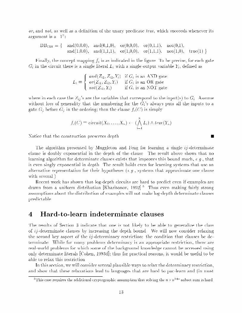
The �rst two sets of literals introduce two sets of depth-1 indeterminate variables: the Xk'scorrespond to possible values for the variables x1; : : : ; xn over which � is de�ned, and theVij 's correspond to values that can be assigned to the literals lij that appear in �. The thirdset of literals ensures that if lij = xk then Vij = Xk, and that if lij = xk then Vij and Xk arecomplements; this conjunction thus ensures that the Vij 's have values consistent with someassignment to the xi's. Finally, the last conjunction of literals ensures that the values givento the Vij 's are such that every clause in � succeeds: i.e., that � is satis�ed.Thus we conclude that � is satis�able i� the clause CSAT succeeds on the instance e�,and hence that determining whether CSAT succeeds must be NP-hard.Finally, notice that the boolean predicate requires two facts to de�ne; the sat predicaterequires seven facts to de�ne; and (since each linkk predicate requires at most 2n � 2 � 2 = 8nfacts to de�ne) the link predicates together require only 8n2 facts to de�ne. Hence jjDBjj isbounded by a polynomial in n. It is also clear that CSAT is of size polynomial in n. Thiscompletes the proof.Therefore, in the remainder of this section, we will consider the learnability of languagesstrictly more restrictive than k-Depth. We will �rst consider the learnability of clauses witha bounded number of \free variables".4.2 Clauses with k free variablesLet the free variables of a clause be those variables that appear in the body of the clausebut not in the head. One reasonable restriction to impose is to consider clauses with onlya small number of free variables. This restriction is analogous to that imposed by Haussler[1989].We will consider now the learnability of the language k-Free, de�ned to be all non-recursive clauses containing at most k free variables. Notice that clauses in k-Free arenecessarily of depth at most k; also restricting the number of free variables ensures thatclauses can be evaluated in polynomial time. While at �rst glance this language seems to bequite simple, notice that a clause p(X) q(X;Y ) classi�es an example p(a) as true exactlywhen q(a; b1) 2 DB _ : : : _ q(a; br) 2 DB, where b1; : : : ; br are the possible bindingsof the (indeterminate) variable Y . Thus, indeterminate variables allow some \disjunctive"concepts to be expressed by a single clause.As it turns out, we can exploit the expressive power of indeterminate free variables toencode any boolean expression in disjunctive normal form6 using a single k-free clause (overa suitable database). This leads to the following theorem.Theorem 11 For any constants a � 2 and k � 1, if the language family k-Free[a-DB] ispredictable, then Dnf is predictable.Proof: As in Theorem 9, the statement of the theorem follows directly from a single reduc-tion:6Recall that boolean formulae of the form WiVj lij are said to be in disjunctive normal form. We denotethis language as Dnf, with the size measure for examples being the number of variables (i.e., the lengthof a bit vector encoding an assignment) and the size measure for a formula being the number of literals itcontains. 15

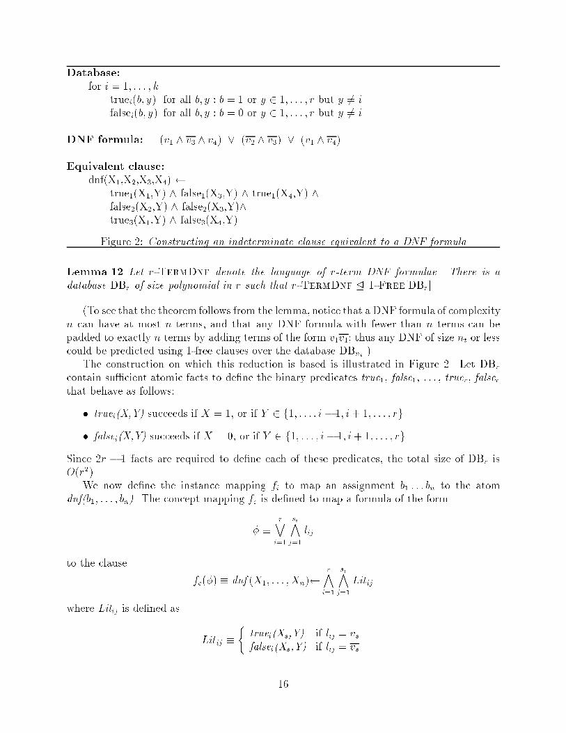
Database:for i = 1; : : : ; ktruei(b; y) for all b; y : b = 1 or y 2 1; : : : ; r but y 6= ifalsei(b; y) for all b; y : b = 0 or y 2 1; : : : ; r but y 6= iDNF formula: (v1 ^ v3 ^ v4) _ (v2 ^ v3) _ (v1 ^ v4)Equivalent clause:dnf(X1,X2,X3,X4) true1(X1,Y) ^ false1(X3,Y) ^ true1(X4,Y) ^false2(X2,Y) ^ false2(X3,Y)^true3(X1,Y) ^ false3(X4,Y).Figure 2: Constructing an indeterminate clause equivalent to a DNF formulaLemma 12 Let r-TermDnf denote the language of r-term DNF formulae. There is adatabase DBr of size polynomial in r such that r-TermDnf � 1-Free[DBr](To see that the theorem follows from the lemma, notice that a DNF formula of complexityn can have at most n terms, and that any DNF formula with fewer than n terms can bepadded to exactly n terms by adding terms of the form v1v1; thus any DNF of size nt or lesscould be predicted using 1-free clauses over the database DBnt.)The construction on which this reduction is based is illustrated in Figure 2. Let DBrcontain su�cient atomic facts to de�ne the binary predicates true1, false1, : : : , truer, falserthat behave as follows:� truei(X,Y) succeeds if X = 1, or if Y 2 f1; : : : ; i� 1; i+ 1; : : : ; rg.� falsei(X,Y) succeeds if X = 0, or if Y 2 f1; : : : ; i� 1; i+ 1; : : : ; rg.Since 2r � 1 facts are required to de�ne each of these predicates, the total size of DBr isO(r2).We now de�ne the instance mapping fi to map an assignment b1 : : : bn to the atomdnf(b1; : : : ; bn). The concept mapping fc is de�ned to map a formula of the form� � r_i=1 sij=1 lijto the clause fc(�) � dnf (X1; : : : ;Xn) ri=1 sij=1Lit ijwhere Litij is de�ned as Lit ij � ( truei(Xs,Y) if lij = vsfalsei(Xs,Y) if lij = vs16

Clearly finst(e) and fc(�) are of the size as e and � respectively; since DBr is also ofpolynomial size, this reduction is polynomial.Next, notice that in fc(�) there is only one variable Y not appearing in the head, and (ifthe clause fc(�) is to succeed) it can be bound to only the r values 1; : : : ; r. Thus if � is truefor an assignment b1 : : : bn, then some term Ti = Vsij=1 lij must be true; in this case Vsij=1 Lit ijsucceeds (with Y bound to the value i) and Vsi0j=1 Lit i0j for every i0 6= i also succeeds withY bound to i. On the other hand, if � is false for an assignment, then each Ti fails, andhence for every possible binding of Y some conjunction Vsij=1 Lit ij will fail. Thus conceptmembership is preserved by the mapping.It also should be noted that every clause in 1-Free[DBr] can be translated into an r-termDNF expression; thus Lemma 12, together with existing hardness results for pac-learningk-term DNF [Kearns et al., 1987], leads to the following result.Observation 13 For a � 2 the language family 1-Free[a-DB] is not pac-learnable.It is straightforward to obtain a number of other similar representation dependent hard-ness results for pac-learning clauses in k-Free, somewhat along the lines of Theorem 1 ofKietz [1993]. However, if one accepts the conjecture that learning DNF is hard, then theseare of limited interest, given Theorem 11; hence we will not develop such results here. Weturn instead to another question: whether there are languages in k-Free that are harder tolearn than DNF. The answer to this question is no:Theorem 14 If DNF is predictable then for all constants a and k, the language familyk-Free[a-DB] is uniformly predictable.Proof: It su�ces to show that for all constants a and k and every background theoryDB 2 a-DB k-Free[DB] � Dnfsince if this reduction holds, one could use the hypothesized prediction algorithm for Dnfto predict k-Free[DB]. Below we will give such a reduction for an arbitrary database DB.Let C be a clause in k-Free[DB]. The predicate symbol and arity of the head of C canbe determined from any of the positive examples, and because we assume that DB containsan equality predicate, one can also assume that all of the variables in the head of C aredistinct.7 Thus the head of C can be determined from the examples.Notice also that each clause has at most ne+k variables, and hence there are only (ne+k)aa-tuples of variables that could serve as arguments to a literal. Let the background databaseDB be of size nb. Since the database DB contains at most nb predicate symbols, there areat most nb � (ne + k)a possible literals B1; : : : ; Bnb�(ne+k)a that can appear in the body of ak-Free clause.7More precisely, for every target clause C in which the variables in the head are are not distinct, thereis an equivalent clause C 0 in which the variables in the head of C 0 are distinct, and the necessary equalityconstraints are represented by conditions in the body ofC 0. It is easy to see that C 0 need be only polynomiallylarger than C'. 17

Now, let C = A Bc1 ^ : : : ^ Bcl be a clause in k-Free[DB]. Recall that C covers anexample e i� there exists some substitution � such thatBc1��e 2 DB ^ : : : ^ Bcl��e 2 DB (1)where �e is the most general substitution such that A�e = e. However, since the backgroundtheory DB is of size nb and all predicates are of arity a or less, there are at most anb constantsin DB, and hence only (anb)k possible substitutions �1; : : : ; �(anb)k to the k free variables.Thus, let us introduce the boolean variables vij where i ranges from one to nb � (ne + k)aand represents a literal, and j ranges from one to (anb)k and represents a substitution. Noticethat the size of this set of variables is polynomial in ne and ne. We will de�ne the instancemapping fi(e) of an example e to return an assignment �e to these variables as follows: vijwill be true in �e if and only if Bi�j�e 2 DB. Finally, let the concept mapping fc(C) map aclause C = A Bc1 ^ : : : ^Bcl to the DNF formulafc(C) � (anb)k_j=1 li=1 vcijSince both (anb)k and l are polynomial (in ne, nb, and nt) the formula fc(C) is of polynomialsize. It also can be veri�ed that fc(C) is true exactly when Equation 1 is true, and hencethese mapping preserve concept membership. This completes the reduction and the proof.The predictability of DNF has been an open problem in computational learning theoryfor several years. Thus, while this result does not actually settle the question of whetherindeterminate clauses are predictable, it does show that answering the question will requirea substantial theoretical advance.4.3 Clauses with bounded indeterminacyIf one believes that DNF is hard to predict, then the result above is negative; however, it doessuggest some possible restrictions that might lead to learnable languages. The �rst restrictionsuggested by this result is based on the observation that the \degree of indeterminacy" of aclause is closely related to the number of terms in the DNF formula that is needed to emulateit, and that k-term DNF is predictable for any �xed k. Hence, it may be that boundingthe number of possible substitutions associated with a clause will lead to a predictablelanguage. Such a result would be useful: intuitively, this would show that predictability (ifnot learnability) decreases gradually as indeterminacy is introduced to a language.In this section, we will investigate such a restriction. It turns out that this intuitionis correct: in particular, the result of Theorem 6 can be extended to a certain languageof clauses with bounded indeterminacy. This gives us a positive learnability result in theweaker model of predictability. We will �rst present a fairly general version of this result,and then consider some concrete instantiations of the general result.18

4.3.1 Bounding the indeterminacy of a clauseWe will want to talk about clauses that are almost, but not quite, deterministic; hence thefollowing de�nition.De�nition 15 (E�ectively k-indeterminate) A language Lang[DB] is called e�ectivelyk-indeterminate (with respect toX) i� there is a polytime computable procedure SUBST(e;DB)that, given any e 2 X, computes a set of substitutions f�1; : : : ; �lg having these properties:� the number of substitutions l is bounded above by k,� for every C 2 Lang[DB], if e is in the extension of C, then every most generalsubstitution �0 that proves e to be in the extension of C is included in the set of �i'sgenerated by SUBST.Note that since duplications are allowed among the �i's (i.e., it might be that �i = �j forsome i 6= j) we can assume without loss of generality that l = k.Informally, a language is k-indeterminate if given an instance e, one can produce a smallset of candidate substitutions that su�ce for all the theorem-proving that might be necessary.As one example of such a language, ij-determinate clauses are e�ectively 1-indeterminate:here, SUBST can be implemented by using a Prolog-style theorem prover to generate thesingle substitution that proves e to be in the extension of C. Some additional examples aregiven in Section 4.3.2.The following property will also be important:De�nition 16 (Polynomial literal support) A language family Lang[DB] has polyno-mial literal support i� for every Xne and every DB 2 DB there is a set of literals LIT anda partial order � on LIT such that� the cardinality of LIT is polynomial in ne and jjDBjj;� Lang[DB] is exactly those clauses A B1 ^ : : :^Br, where A is �xed, all the Bi's aremembers of LIT, and the body of the clause satis�es the following restriction: if Bi�Bjand Bj is in body of the clause, then Bi also is in the body of the clause and appearsto the left of Bj.One example of a language with polynomial literal support is the language of ij-determinateclauses: in this case, the polynomial bound on the number of literals in a clause can be ob-tained by a simple counting argument [Muggleton and Feng, 1992], and the ordering functionis the relationship Bi�Bj i� the input variables of Bj are bound by BiThis de�nition in fact generalizes of a key property that, together with determinism, makesij-determinate clauses pac-learnable. The language of k-free clauses also has polynomialliteral support; in this case, the ordering function might be a constant function, or mightbe used to ensure that clauses are \linked" in such a way as to reduce indeterminacy. The19

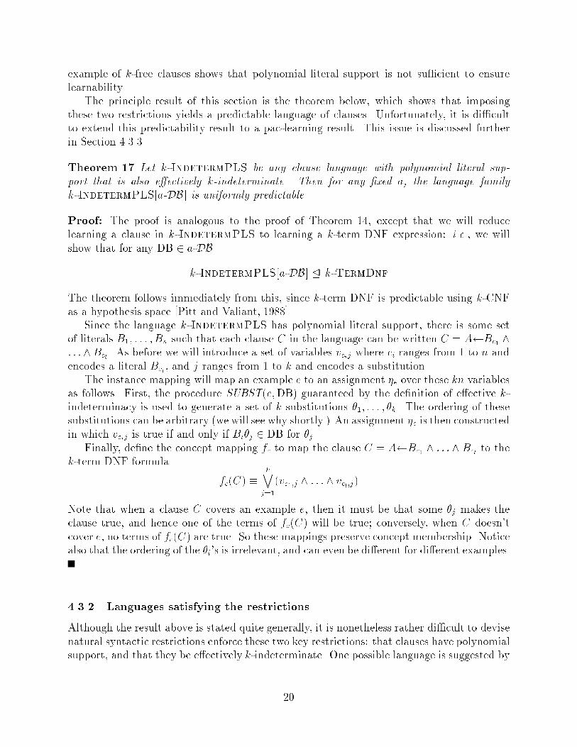
example of k-free clauses shows that polynomial literal support is not su�cient to ensurelearnability.The principle result of this section is the theorem below, which shows that imposingthese two restrictions yields a predictable language of clauses. Unfortunately, it is di�cultto extend this predictability result to a pac-learning result. This issue is discussed furtherin Section 4.3.3.Theorem 17 Let k-IndetermPLS be any clause language with polynomial literal sup-port that is also e�ectively k-indeterminate. Then for any �xed a, the language familyk-IndetermPLS[a-DB] is uniformly predictable.Proof: The proof is analogous to the proof of Theorem 14, except that we will reducelearning a clause in k-IndetermPLS to learning a k-term DNF expression: i.e., we willshow that for any DB 2 a-DBk-IndetermPLS[a-DB] � k-TermDnfThe theorem follows immediately from this, since k-term DNF is predictable using k-CNFas a hypothesis space [Pitt and Valiant, 1988].Since the language k-IndetermPLS has polynomial literal support, there is some setof literals B1; : : : ; Bn such that each clause C in the language can be written C = A Bc1 ^: : : ^Bcl . As before we will introduce a set of variables vcij where ci ranges from 1 to n andencodes a literal Bci , and j ranges from 1 to k and encodes a substitution.The instance mapping will map an example e to an assignment �e over these kn variablesas follows. First, the procedure SUBST(e;DB) guaranteed by the de�nition of e�ective k-indeterminacy is used to generate a set of k substitutions �1; : : : ; �k. The ordering of thesesubstitutions can be arbitrary (we will see why shortly.) An assignment �e is then constructedin which vcij is true if and only if Bi�j 2 DB for �j.Finally, de�ne the concept mapping fc to map the clause C = A Bc1 ^ : : : ^ Bcl to thek-term DNF formula fc(C) � k_j=1(vc1;j ^ : : : ^ vcl;j)Note that when a clause C covers an example e, then it must be that some �j makes theclause true, and hence one of the terms of fc(C) will be true; conversely, when C doesn'tcover e, no terms of fc(C) are true. So these mappings preserve concept membership. Noticealso that the ordering of the �i's is irrelevant, and can even be di�erent for di�erent examples.4.3.2 Languages satisfying the restrictionsAlthough the result above is stated quite generally, it is nonetheless rather di�cult to devisenatural syntactic restrictions enforce these two key restrictions: that clauses have polynomialsupport, and that they be e�ectively k-indeterminate. One possible language is suggested by20

the proof of Theorem 14, which shows that any language k-Free[DB] is e�ectively jjDBjjk-indeterminate. Thus the language family of k-free clauses over databases of constant size lis predictable. Thus letting DBl denote the set of databases of size less than or equal to l:Observation 18 For �xed k and l the language family k-Free[DBl] is uniformly pre-dictable.Note however that the time complexity of the most natural prediction algorithm (whereone predicts k-term DNF using k-CNF) is O(nelk), which seems rather high for a practicalalgorithm. Also, restricting the size of the background database is a rather severe restriction.Another possibly more useful way of de�ning a language meeting the restrictions aboveis as follows.� First, specify a tuple of ne variables. The head of every clause in the language willhave as its arguments the tuple T .For instance, in learning family relationships like grandfather or nephew, one might �xthe arguments to be the two variables X and Y , in that order.� Next, specify some small set of output literals S = fL1; : : : ; Lcg and an ordering func-tion �S such that each output literal can have at most d possible bindings, when usedin a clause in a manner consistent with �S.Continuing the example given above (in which X and Y are the arguments to the headof the clause), one might specify the following set of c = 6 output literalsS = f L1 = parent(X ;A); L2 = parent(Y ;B);L3 = parent(A;C ); L4 = parent(B ;D);L5 = spouse(X ;E ); L6 = spouse(Y ;F ) gtogether with the following ordering �S:L1 �S L3L2 �S L4Given this ordering constraint, literals L1, L2, L3 and L4 can have at most two bindings(assuming that a person has at most two parents) and literals L5 and L6 can have atmost one binding (assuming each person has only one spouse.) Thus, for this set S,we have d = 2.� Finally, de�ne the language S-Output to be the set of clauses that have heads withthe argument list T and bodies that contain output literals selected from the set S,and used in an order consistent with �S.It is easy to show that a clause in S-Output is e�ectively (jSj �d)-indeterminate: the proce-dure for generating substitutions is simply to backtrack to generate all possible substitutionsfor the free variables in the literal set S. Also, for databases with a �xed arity a the languageS-Output has polynomial literal support, since it has at most ajSj free variables. Hence:21

Observation 19 For every constants a, c, and d, and every literal set S, S-Output[a-DB]is uniformly predictable, provided that jSj < c, and every literal in S can have at most dbindings.The time complexity of the k-CNF based prediction algorithm is O(necd).It should be noted that there is no a priori way to choose the literal set S and orderingfunction �S. Thus in practice, specifying a language S-Output requires additional userinput. For example, in the family relationship learning problem given above, the user hadto specify (in addition to the examples and the background database DB)� the pair of variables X;Y that must appear in the head of the hypothesis clause;� the set of indeterminate literals S = fparent(A;X ); : : : ; g that can appear in a hypoth-esis clause;� the ordering function �S.In this respect the clause language S-Output di�ers from i-DepthDeterm and k-Free,which require little user input to specify.This result also can be generalized somewhat. One generalization is based on the fact thatij-determinate clauses also have polynomial literal support. It is thus possible to combine thelanguage of ij-determinate clauses with the language S-Output to obtain a new predictablelanguage, of clauses of the formA B1 ^ : : : ^Br ^D1 ^ : : : ^Dswhere A B1 ^ : : : ^ Br is ij-determinate and A D1 ^ : : : ^Ds is S-Output. This resultprovides one way of introducing a small amount of non-determinism into the language ofij-determinate clauses without making prediction intractable.4.3.3 Further discussionIt should be emphasized that although this is a positive result, there are a number of reasonswhy the result is rather weak. First, we have not shown the language to be pac-learnable, onlyto be predictable; thus there is no way of obtaining a clause that accurately approximates thetarget clause. This is a disadvantage if the ultimate goal is to integrate the result of learningwith a reasoning system based on logic programs. Furthermore, the result appears to bedi�cult to extend to pac-learnability, for two reasons: �rst, because k-term DNF is hard topac-learn, and second, because the concept mapping used to reduce clause learning to k-termDNF cannot be easily reversed. The latter fact means that even if the prediction algorithmused for k-term DNF yields hypotheses that can be easily converted to logic programs (see,for example, [Blum and Singh, 1990], which describes an algorithm that learns k-term DNFwith general DNF) or even for classes of distributions under which k-term DNF is directlylearnable (see, for example, [Li and Vitanyi, 1991]) it may still be impossible to pac-learnclauses from an e�ectively k-indeterminate language with polynomial literal support.A second problem is that all known algorithms for predicting k-term DNF require timeexponential in k. This suggests that only a small amount of indeterminism can be toleratedwithout imposing additional restrictions. For these reasons, we will consider in the nextsection a di�erent restriction on indeterminate clauses.22

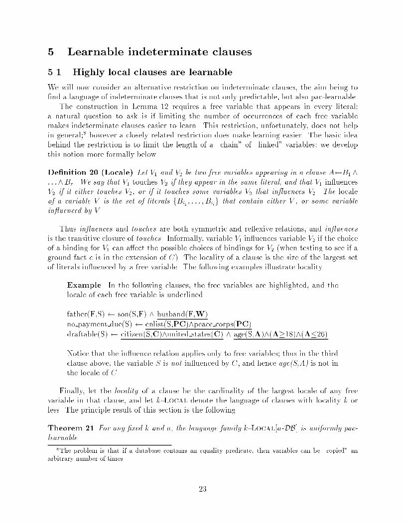
5 Learnable indeterminate clauses5.1 Highly local clauses are learnableWe will now consider an alternative restriction on indeterminate clauses, the aim being to�nd a language of indeterminate clauses that is not only predictable, but also pac-learnable.The construction in Lemma 12 requires a free variable that appears in every literal;a natural question to ask is if limiting the number of occurrences of each free variablemakes indeterminate clauses easier to learn. This restriction, unfortunately, does not helpin general;8 however a closely related restriction does make learning easier. The basic ideabehind the restriction is to limit the length of a \chain" of \linked" variables; we developthis notion more formally below.De�nition 20 (Locale) Let V1 and V2 be two free variables appearing in a clause A B1 ^: : :^Br. We say that V1 touches V2 if they appear in the same literal, and that V1 in uencesV2 if it either touches V2, or if it touches some variables V3 that in uences V2. The localeof a variable V is the set of literals fBi1 ; : : : ; Bilg that contain either V , or some variablein uenced by V .Thus in uences and touches are both symmetric and re exive relations, and in uencesis the transitive closure of touches. Informally, variable V1 in uences variable V2 if the choiceof a binding for V1 can a�ect the possible choices of bindings for V2 (when testing to see if aground fact e is in the extension of C). The locality of a clause is the size of the largest setof literals in uenced by a free variable. The following examples illustrate locality.Example. In the following clauses, the free variables are highlighted, and thelocale of each free variable is underlined.father(F,S) son(S,F) ^ husband(F,W).no payment due(S) enlist(S,PC)^peace corps(PC).draftable(S) citizen(S,C)^united states(C) ^ age(S,A)^(A�18)^(A�26).Notice that the in uence relation applies only to free variables; thus in the thirdclause above, the variable S is not in uenced by C, and hence age(S,A) is not inthe locale of C.Finally, let the locality of a clause be the cardinality of the largest locale of any freevariable in that clause, and let k-Local denote the language of clauses with locality k orless. The principle result of this section is the following.Theorem 21 For any �xed k and a, the language family k-Local[a-DB] is uniformly pac-learnable.8The problem is that if a database contains an equality predicate, then variables can be \copied" anarbitrary number of times. 23

Proof: Let S+; S� be a sample labeled by the k-local clause A B1 ^ : : : ^ Bl. As in theproof of Theorem 17, one can assume that predicate symbol and arity of A are known, andthat the arguments to A are ne distinct variables. As every new literal in the body canintroduce at most a new variables, any size k locale can contain at most ne + ak distinctvariables. Also note that there are at most nb distinct predicates in the database DB. Sinceeach literal in a locality has one predicate symbol and at most a arguments, each of which isone of the ne + ak variables, there are only nb(ne + ak)a di�erent literals that could appearin a locality, and hence at most p = (nb(ne + ak)a)k di�erent9 localities of length k. Let usdenote these localities as LOC 1; : : : ;LOC p. Note that for constant a and k, the number ofdistinct localities p is polynomial in ne and nb.Now, notice that every clause C of locality k can be written in the formA LOC i1 ; : : : ;LOC irwhere each LOC ij is one of the p possible locales, and no free variable appears in morethan one of the LOC ij 's. Since no free variables are shared between locales, the di�erentlocales do not interact, and hence e 2 ext (C;DB) exactly when e 2 ext(A LOC i1;DB) and: : : and e 2 ext(A LOC ir ;DB). In other words, C can be decomposed into a conjunctionof components of the form A LOC ij . One can thus use Valiant's [1984] technique formonomials to learn C.In a bit more detail, the following algorithm will pac-learn k-local clauses. The learnerinitially hypothesizes the most speci�c k-local clause, namelyA LOC 1; : : : ;LOC pThe learner then examines each positive example e in turn, and deletes from its hypothesisall LOC i such that e 62 ext (A LOC i;DB). (Note that e is in this extension exactly when9� : DB ` LOC i�e� where �e is the most general substitution such that A�e = e. To see thatthis condition can be checked in polynomial time, recall that � can contain at most ak freevariables, and DB can contain at most anb constants; hence at most (anb)ak substitutions �need be checked, which is polynomial.) Following the argument used for Valiant's procedure,this algorithm will pac-learn the target concept.Again, this result can be extended somewhat; for example, there is pac-learning algorithmfor the language of clauses of the formA B1 ^ : : : ^Br ^D1 ^ : : : ^Dswhere A B1 ^ : : : ^Br is ij-determinate and A D1 ^ : : : ^Ds is k-local.5.2 The expressive power of local clausesTheorem 21 is a positive result; it shows that k-local clauses can be e�ciently learned in areasonable formal model. The importance of this result, however, depends a great deal on9Up to renaming of variables. 24

the usefulness of k-local clauses as a representation language; we note that k-local clauses,unlike ij-determinate clauses, do not seem to correspond very well to the sorts of clausestypically used in logic programs for list manipulation and other programming tasks. In thissection, we will attempt to evaluate the usefulness of locality as a bias.5.2.1 Experimental resultsOne way is to evaluate a bias is empirically, by applying a learning system that uses that biasto benchmark problems. Some preliminary experiments of this sort are reported elsewhere[Cohen, 1993d]. In these experiments, several di�erent versions of the experimental ILPsystem Grendel were constructed, each of which learned programs made up of clauses froma di�erent clause language. Among the clause languages considered were ij-determinateand k-local clauses. These di�erent versions of Grendel were then compared on a set ofeight benchmark problems taken from the literature. These experiments con�rmed that ij-determinacy is useful on many problems, notably in learning simple recursive programs likeappend and list. However, on two of the eight benchmarks, signi�cantly better results wereobtained by relaxing the determinacy restriction and imposing instead a locality restriction.Thus, the results suggest that it is sometimes important to relax the determinacy restriction,and indicate that locality is, at least in some cases, a useful way of doing so.5.2.2 Locality generalizes ij-determinacyA second way to evaluate the usefulness of locality is to formally analyze the expressivepower of k-local clauses. The easiest way to do this is by comparing k-Local to otherlanguages. For instance, any clause with locality k clearly must have depth of k + 1 or less;thus k-Local is also a restriction of the language of clauses of constant depth. However,the language k-Local is incomparable to the language of clauses with a bounded numberof free variables. To see this, note that the construction used in Lemma 12 is a length nclause with a single free variable that has locality n, while similarly the clausep(X) q1(X;Y1) ^ : : : ^ qn(X;Yn)has locality one, but n free variables. To summarize, k-Local � (k + 1)-Depth, but forall k0, k-Local 6� k0-Free and k-Free 6� k0-Local.A more interesting question is the relationship of k-local clauses to ij-determinate clauses.Clearly, since k-local clauses can include indeterminate literals, some k-local clauses are notij-determinate. It is also the case that determinate clauses with bounded depth can haveunbounded locality. As an example, consider the clausep(X) successor(X;Y) ^ q1(Y) ^ : : : ^ qn(Y)However, there is a surprising relationship between the two languages: it turns out that everyij-determinate clause can be rewritten as a clause with bounded locality, where the boundon the locality is a function only of i and j. Thus, in a very reasonable sense, the language ofclauses of constant locality is a strict generalization of the language of determinate clausesof constant depth.More precisely, the following relationship holds between these languages.25

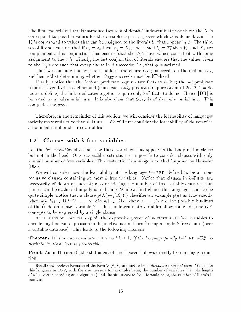
Theorem 22 For every DB 2 a-DB, every d, and every clause C 2 d-DepthDeterm[DB],there is clause C 0 2 k-Local[DB] such that C 0 is equivalent to C and jjC 0jj � kjjCjj, wherek = ad+1.Proof: Let C = A B1 ^ : : : ^ Br be a clause. We will say that literal Bi directly supportsliteralBj i� some output variable of Bi is an input variable ofBj , and that literalBi indirectlysupports Bj i� Bi directly supports Bj , or if Bi directly supports some Bk that indirectlysupports Bj. (Thus \indirectly supports" is the transitive closure of \directly supports".)Now, for each Bi in the body of C, let LOC i be the conjunctionLOC i = Bj1 ^ : : : ^Bjki ^Biwhere the Bj 's are all of the literals of C that support Bi, either directly or indirectly,appearing in the same order that they appeared in C. Next, let us introduce for i = 1; : : : ; ra substitution �i = fY = Yi : Y is a variable occurring LOC i but not in AgWe can then de�ne LOC 0i = LOC i�i; the e�ect of this last step is that LOC 01; : : : ;LOC 0r arecopies of LOC 1; : : : ;LOC r in which variables have been renamed so that the free variablesof LOC 0i1 are di�erent from the free variables of LOC 0i2 . Finally, let C 0 be the clauseA LOC 01 ^ : : :LOC 0rAn example of this construction is given in Figure 3. We suggest that the reader refer to theexample at this point.We claim that C 0 is k-local, for k = ad+1, that C 0 is at most k times the size of C, andfurthermore that if C is determinate, then C 0 has the same extension as C. In the remainderof the proof, we will establish these claims.To establish the �rst two claims (that C 0 is k-local and at most k times the size of C fork = ad+1) it is su�cient to show that the number of literals in every LOC 0i (or equivalently,every LOC i) is bounded by k. To establish this, let us de�ne N(d) to be the maximumnumber of literals in any LOC i corresponding to a Bi with input variables at depth d or less.Clearly for any DB 2 a-DB and C 2 d-DepthDeterm[DB], the function N(d) is an upperbound on k.The function N(d) is bounded by the following lemma.Lemma 23 For any DB 2 a-DB, N(d) �Pdi=0 ai (� ad+1).Proof of lemma: By induction on d. For d = 0, no literals will support Bi, and hence eachlocality LOC i will contain only the literal Bi, and N(0) = 1.Now assume that the lemma holds for d�1 and consider a literal Bi with inputs at depthd. Notice that LOC i can be no larger than the conjunction0@ ^j:Bj directly supports Bi LOC j1A ^ Bi26

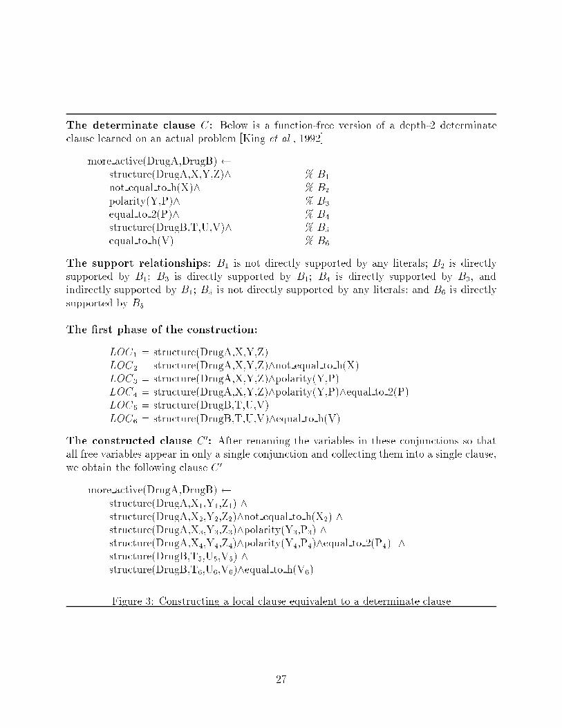
The determinate clause C: Below is a function-free version of a depth-2 determinateclause learned on an actual problem [King et al., 1992].more active(DrugA,DrugB) structure(DrugA,X,Y,Z)^ % B1not equal to h(X)^ % B2polarity(Y,P)^ % B3equal to 2(P)^ % B4structure(DrugB,T,U,V)^ % B5equal to h(V). % B6The support relationships: B1 is not directly supported by any literals; B2 is directlysupported by B1; B3 is directly supported by B1; B4 is directly supported by B3, andindirectly supported by B1; B5 is not directly supported by any literals; and B6 is directlysupported by B5.The �rst phase of the construction:LOC 1 = structure(DrugA,X,Y,Z)LOC 2 = structure(DrugA,X,Y,Z)^not equal to h(X)LOC 3 = structure(DrugA,X,Y,Z)^polarity(Y,P)LOC 4 = structure(DrugA,X,Y,Z)^polarity(Y,P)^equal to 2(P)LOC 5 = structure(DrugB,T,U,V)LOC 6 = structure(DrugB,T,U,V)^equal to h(V)The constructed clause C 0: After renaming the variables in these conjunctions so thatall free variables appear in only a single conjunction and collecting them into a single clause,we obtain the following clause C 0.more active(DrugA,DrugB) structure(DrugA,X1,Y1,Z1) ^structure(DrugA,X2,Y2,Z2)^not equal to h(X2) ^structure(DrugA,X3,Y3,Z3)^polarity(Y3,P3) ^structure(DrugA,X4,Y4,Z4)^polarity(Y4,P4)^equal to 2(P4) ^structure(DrugB,T5,U5,V5) ^structure(DrugB,T6,U6,V6)^equal to h(V6).Figure 3: Constructing a local clause equivalent to a determinate clause27

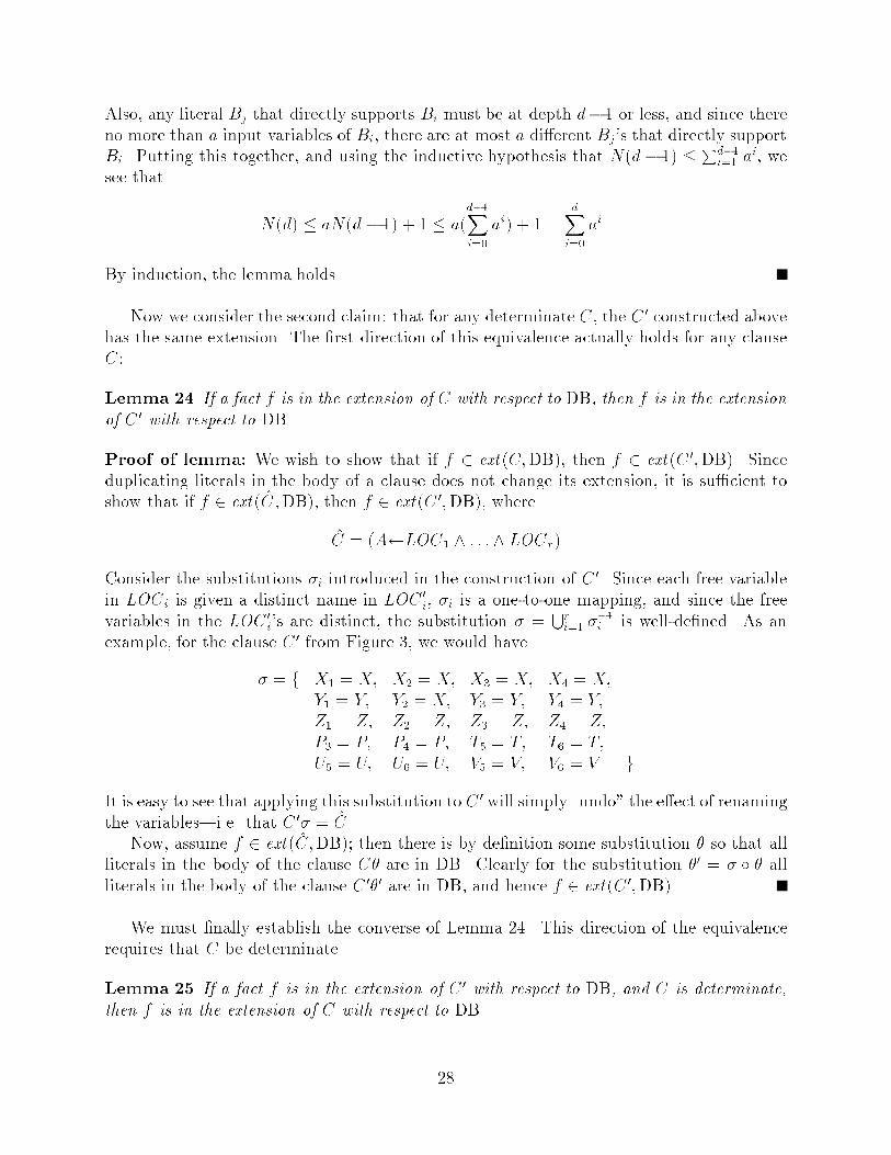
Also, any literal Bj that directly supports Bi must be at depth d� 1 or less, and since thereno more than a input variables of Bi, there are at most a di�erent Bj's that directly supportBi. Putting this together, and using the inductive hypothesis that N(d � 1) � Pd�1i=1 ai, wesee that N(d) � aN(d � 1) + 1 � a(d�1Xi=0 ai) + 1 = dXi=0 aiBy induction, the lemma holds.Now we consider the second claim: that for any determinate C, the C 0 constructed abovehas the same extension. The �rst direction of this equivalence actually holds for any clauseC:Lemma 24 If a fact f is in the extension of C with respect to DB, then f is in the extensionof C 0 with respect to DB.Proof of lemma: We wish to show that if f 2 ext (C;DB), then f 2 ext (C 0;DB). Sinceduplicating literals in the body of a clause does not change its extension, it is su�cient toshow that if f 2 ext (C;DB), then f 2 ext (C 0;DB), whereC = (A LOC 1 ^ : : : ^ LOC r)Consider the substitutions �i introduced in the construction of C 0. Since each free variablein LOC i is given a distinct name in LOC 0i, �i is a one-to-one mapping, and since the freevariables in the LOC 0i's are distinct, the substitution � = Sri=1 ��1i is well-de�ned. As anexample, for the clause C 0 from Figure 3, we would have� = f X1 = X; X2 = X; X3 = X; X4 = X;Y1 = Y; Y2 = X; Y3 = Y; Y4 = Y;Z1 = Z; Z2 = Z; Z3 = Z; Z4 = Z;P3 = P; P4 = P; T5 = T; T6 = T;U5 = U; U6 = U; V5 = V; V6 = V gIt is easy to see that applying this substitution to C 0 will simply \undo" the e�ect of renamingthe variables|i.e. that C 0� = C.Now, assume f 2 ext (C;DB); then there is by de�nition some substitution � so that allliterals in the body of the clause C� are in DB. Clearly for the substitution �0 = � � � allliterals in the body of the clause C 0�0 are in DB, and hence f 2 ext (C 0;DB).We must �nally establish the converse of Lemma 24. This direction of the equivalencerequires that C be determinate.Lemma 25 If a fact f is in the extension of C 0 with respect to DB, and C is determinate,then f is in the extension of C with respect to DB.28

Proof of lemma: If f 2 ext (C 0;DB), then there must be some �0 that proves this. Let usde�ne a variable Yi in C 0 to be a \copy" of Y 2 C if Yi is a renaming of Y (i.e., if Yi��1i = Yfor the �i de�ned in the lemma above). Certainly if C is determinate then C 0 is determinate,and it is easy to show that for a determinate C 0, �0 must map every copy of Y to the sameconstant tY . (This is most easily proved by picking two copies Yi and Yj of Y and then usinginduction over the depth of Y to show that they must be bound to the same constant. Forvariables of depth d = 0, the statement is vacuously true, since there are no copies of depthzero variables. For variables of depth d > 0, consider the literals Bi and Bj that containYi and Yj as output variables, and apply the inductive hypothesis to show that their inputvariables must have the same bindings; together with the determinism of C, this shows thatYi and Yj must be bound to the same constant.)Hence, let us de�ne the substitution� = fY = tY : copies of Y in C 0 are bound to tY by �0gClearly, for all i : 1 � i � r, LOC i� = LOC i�0; hence if �0 proves that f 2 ext (C 0;DB) then� proves that f 2 ext (C;DB).We have now established that C 0 is k-local, of bounded size, and is equivalent to C. Thisconcludes the proof of the theorem.We note that the proof technique used in Theorem 22 is similar to that used by D�zeroski,Muggleton and Russell [1992] to show that ij-determinate clauses are learnable; in particular,D�zeroski, Muggleton and Russell showed that a ij-determinate clause can be rewritten as aconjunction of boolean propositions, each of which corresponds closely to the conjunctionsLOC 01; : : : ;LOC 0r introduced in the proof above.Finally, although we have shown that ij-determinate clauses have locality bounded by aconstant, it should be observed that the constant is fairly large: for example, for i = j = 3,the bound on locality would be k = 34 = 81. Hence the algorithm of Theorem 21 need notbe the best algorithm for learning ij-determinate clauses.6 Extensions to multiple-clause programsSo far, all of our results have been for programs containing a single clause. We will nowconsider extending the results presented above to programs that contain more than oneclause. This is an important topic, because many practical systems learn programs containingmultiple clauses; further understanding of the limitations of such systems would clearly beuseful.Still considering non-recursive programs over a �xed database, an immediate result isthat even with severe restrictions, learning an arbitrary logic program is cryptographicallyhard. (We will use, in this proof, the usual semantics for logic programs [Lloyd, 1987].)Theorem 26 For a � 1, the language of nonrecursive multiple-clause programs containingclauses from the following language families are not polynomially predictable, under crypto-graphic assumptions: 29

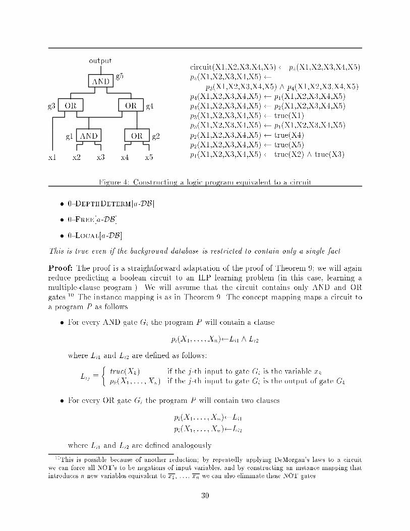
g3 g1 g5 g4g2outputx5x4x3x2x1 AND OROR ORAND circuit(X1,X2,X3,X4,X5) p5(X1,X2,X3,X4,X5).p5(X1,X2,X3,X4,X5) p3(X1,X2,X3,X4,X5) ^ p4(X1,X2,X3,X4,X5).p4(X1,X2,X3,X4,X5) p1(X1,X2,X3,X4,X5).p4(X1,X2,X3,X4,X5) p2(X1,X2,X3,X4,X5).p3(X1,X2,X3,X4,X5) true(X1).p3(X1,X2,X3,X4,X5) p1(X1,X2,X3,X4,X5).p2(X1,X2,X3,X4,X5) true(X4).p2(X1,X2,X3,X4,X5) true(X5).p1(X1,X2,X3,X4,X5) true(X2) ^ true(X3).Figure 4: Constructing a logic program equivalent to a circuit� 0-DepthDeterm[a-DB]� 0-Free[a-DB]� 0-Local[a-DB]This is true even if the background database is restricted to contain only a single fact.Proof: The proof is a straightforward adaptation of the proof of Theorem 9; we will againreduce predicting a boolean circuit to an ILP learning problem (in this case, learning amultiple-clause program.) We will assume that the circuit contains only AND and ORgates.10 The instance mapping is as in Theorem 9. The concept mapping maps a circuit toa program P as follows.� For every AND gate Gi the program P will contain a clausepi(X1; : : : ;Xn) Li1 ^ Li2where Li1 and Li2 are de�ned as follows:Lij � ( true(Xk) if the j-th input to gate Gi is the variable xkpk(X1; : : : ;Xn) if the j-th input to gate Gi is the output of gate Gk� For every OR gate Gi the program P will contain two clausespi(X1; : : : ;Xn) Li1pi(X1; : : : ;Xn) Li2where Li1 and Li2 are de�ned analogously.10This is possible because of another reduction; by repeatedly applying DeMorgan's laws to a circuitwe can force all NOT's to be negations of input variables, and by constructing an instance mapping thatintroduces n new variables equivalent to x1, : : : , xn we can also eliminate these NOT gates.30

� Finally, P contains a single clausecircuit(X1; : : : ;Xn) pn(X1; : : : ;Xn)where pn is the gate whose output is the output of the circuit.An example of this construction is shown in Figure 4.It is easy to verify that this construction reduces learning circuits to learning multiple-clause programs of any of the types named in the theorem over the database DB = ftrue(1 )g.Since arbitrary logic programs are hard to learn, we will henceforth restrict ourselves tocases in which the heads of all the clauses in the program have the same predicate symbol andarity; this restriction has been made by a number of practical learning systems [Quinlan,1990; Muggleton and Feng, 1992; Pazzani and Kibler, 1992; Cohen, 1991]. We will callsuch programs multiple-clause predicate de�nitions. For this case, the semantics of ourrepresentation remains simple: a multiple clause predicate de�nition is simply a set of clausesP = fC1; : : : ; Ckg, and the extension of P with respect to a database DB is the union ofthe extensions of the Ci's (again with respect to DB). Again, this coincides with the usualsemantics for non-recursive programs.Many of the preceding results extend immediately to multiple-clause predicate de�nitions;for completeness, we will state these extensions below.Observation 27 For a � 3, the language of multiple-clause predicate de�nitions containingclauses from (log ne)-DepthDeterm[a-DB] are not polynomially predictable, under crypto-graphic assumptions.This follows directly from the non-predictability of single clauses.Observation 28 For any a � 2 and any k � 1, the language of multiple-clause predicatede�nitions containing clauses from k-Free[a-DB] is uniformly predictable if and only if Dnfis predictable.This follows directly from Theorems 11 and 14, and from the fact that the disjunction ofa set of DNF formula is still in DNF.Observation 29 Let k-IndetermPLS be any clause language with polynomial literal sup-port containing only e�ectively k-indeterminate clauses. Then for any �xed a, k andl, the language of multiple-clause predicate de�nitions containing at most l clauses fromk-IndetermPLS[a-DB] is uniformly predictable.This follows directly from Theorem 17 and the fact that the union of l distinct k-termDNF formula, where l is constant, is a (k � l)-term DNF formula.It remains to consider extensions of Theorems 6 and 21, which show the pac-learnability ofij-determinate clauses and k-local clauses respectively. Again, these extensions are straight-forward, based on previous results. The proof of Theorem 6 is based on a invertible reduction31

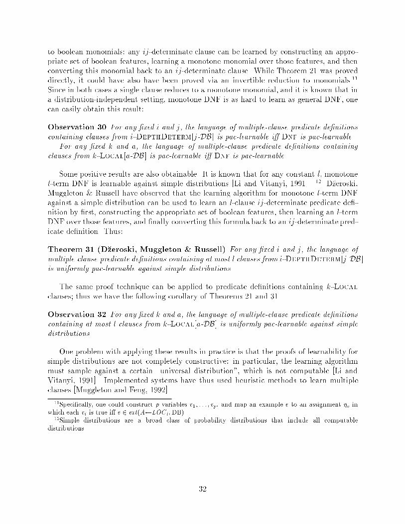
to boolean monomials: any ij-determinate clause can be learned by constructing an appro-priate set of boolean features, learning a monotone monomial over those features, and thenconverting this monomial back to an ij-determinate clause. While Theorem 21 was proveddirectly, it could have also have been proved via an invertible reduction to monomials.11Since in both cases a single clause reduces to a monotone monomial, and it is known that ina distribution-independent setting, monotone DNF is as hard to learn as general DNF, onecan easily obtain this result:Observation 30 For any �xed i and j, the language of multiple-clause predicate de�nitionscontaining clauses from i-DepthDeterm[j-DB] is pac-learnable i� Dnf is pac-learnable.For any �xed k and a, the language of multiple-clause predicate de�nitions containingclauses from k-Local[a-DB] is pac-learnable i� Dnf is pac-learnable.Some positive results are also obtainable. It is known that for any constant l, monotonel-term DNF is learnable against simple distributions [Li and Vitanyi, 1991]. 12 D�zeroski,Muggleton & Russell have observed that the learning algorithm for monotone l-term DNFagainst a simple distribution can be used to learn an l-clause ij-determinate predicate de�-nition by �rst, constructing the appropriate set of boolean features, then learning an l-termDNF over those features, and �nally converting this formula back to an ij-determinate pred-icate de�nition. Thus:Theorem 31 (D�zeroski, Muggleton & Russell) For any �xed i and j, the language ofmultiple-clause predicate de�nitions containing at most l clauses from i-DepthDeterm[j-DB]is uniformly pac-learnable against simple distributions.The same proof technique can be applied to predicate de�nitions containing k-Localclauses; thus we have the following corollary of Theorems 21 and 31.Observation 32 For any �xed k and a, the language of multiple-clause predicate de�nitionscontaining at most l clauses from k-Local[a-DB] is uniformly pac-learnable against simpledistributions.One problem with applying these results in practice is that the proofs of learnability forsimple distributions are not completely constructive: in particular, the learning algorithmmust sample against a certain \universal distribution", which is not computable [Li andVitanyi, 1991]. Implemented systems have thus used heuristic methods to learn multipleclauses [Muggleton and Feng, 1992].11Speci�cally, one could construct p variables v1; : : : ; vp, and map an example e to an assignment �e inwhich each vi is true i� e 2 ext(A LOC i;DB).12Simple distributions are a broad class of probability distributions that include all computabledistributions. 32

XXXXXXXXX """"""������ ��������PPPPPPPPPPPPPHHHHHHHH����������eeee k-Depthn-DepthDetermlog n-DepthDetermk-DepthDeterm S-Output k-Localk-Freek-IndetermPLSFigure 5: Summary of results for single clauses. Above the heavy line are languages that arehard to predict, and below the heavy line are languages that are predictable. All predictablelanguages except k-IndetermPLS are also pac-learnable. Predicting the boxed languagek-Free is equivalent to predicting DNF, an open problem.7 Concluding remarksMost implemented �rst-order learning systems use restricted logic programs to represent con-cepts. An obvious advantage of this representation is that its semantics and complexity aremathematically well-understood; this suggests that learning systems using such logics canalso be mathematically analyzed. This paper has sought to expand the theoretical founda-tions of this sub�eld, inductive logic programming, by formally investigating the learnabilityof restricted logic programs. Most of our analysis is using the model of polynomial pre-dictability introduced by Pitt and Warmuth [1990]. This model encourages analyzing thelearnability of a language by characterizing its expressive power.In this paper we have characterized several extensions of the language of determinateclauses of constant depth [Muggleton and Feng, 1992; D�zeroski et al., 1992]. These resultswill now be summarized.First, via a reduction from log-depth circuits, we showed that a single log-depth deter-minate clause is not pac-learnable.Next, we relaxed the condition of determinacy, and obtained a number of results. Sinceindeterminate clauses of constant depth can be very easily shown to be hard to predict, weconsidered several restrictions of this language. We showed that a clause with k free variablesis as hard to learn as DNF. We also showed that restricting the degree of indeterminacyof a clause leads to predictability (but not pac-learnability) for any clause language with\polynomial literal support".Finally, we showed that restricting the locality of a clause to a constant k leads to pac-learnability. This result is especially interesting because k-local clauses can be shown to be astrict generalization of ij-determinate clauses in the following sense: for �xed i and j, everyij-determinate clause can be rewritten as a clause with locality no greater than ji+1.These results are summarized in Figure 5, which shows the languages considered in this33

paper, partially ordered by their expressive power.13 The results associate with the parenthe-sized languages are from previous work [D�zeroski et al., 1992; Kietz, 1993]; note however thatthe previous results for arbitrary-depth determinate and constant-depth determinate clausesmake representational assumptions that we have relaxed. The analysis associated with theremaining languages is original. The languages below the heavy line are pac-learnable or (inthe case of k-IndetermPLS) polynomially predictable. The languages above the heavy lineare hard to predict, under cryptographic assumptions, as are all supersets of these languages.The language k-free, shown boxed in a dotted line, is predictable i� DNF is predictable; thisis an open question in computational learning theory.In obtaining these results, several previous results from the literature have been extended.Haussler [1989] raises the question of the learnability of existential conjunctive concepts withk variables in a representation-independent (i.e., predictability) setting. It is easy to shownthat every existential conjunctive concept can be expressed by a single indeterminate clause;thus an immediate result of Theorem 17 is that these concepts are in general as hard topredict as DNF.More recently, Kietz [1993] has shown that arbitrary depth determinate clauses are hardto pac-learn, and that constant depth indeterminate clauses are also hard to pac-learn. Theseresults have both been strengthened in a number of ways in this paper: in particular, wehave presented representation-independent hardness results for determinate clauses of onlylog depth, rather than arbitrary depth, and also for indeterminate constant depth clauses.We have also further investigated the learnability of various subclasses of indeterminateclauses. One result of this in-depth investigation has been isolation of an interesting subclassof indeterminate clauses (the class of k-local clauses) that is pac-learnable, and that is a strictgeneralization of the class of ij-determinate clauses.Kietz and D�zeroski [1994] have also investigated the complexity a closely related taskcalled the ILP problem. The \ILP problem" for (`;DB;LangE;LangH) is to �nd, given abackground theory DB 2 DB and a set of examples from LangE, a hypothesis in LangHthat is \consistent" with the examples with respect to the provability relationship `. Onecorollary of Theorem 21 is that the ILP problem for k-local clauses is tractable. The con-nection between our negative results and the ILP problem is somewhat more complex. Asformalized by Kietz and D�zeroski, it is possible to solve the ILP problem in polynomialtime using an algorithm that generates a hypothesis that grows quickly with the numberof examples|for example, if the hypothesis language LangH is su�ciently expressive, onemight hypothesize a lookup table containing all the positive examples. Thus it is possible inprinciple that the ILP problem for a language might be solvable, even if the language is hardto predict. However, by the results of Blumer et. al [1989] and Theorem 4, if a languageLang is not polynomially predictable and algorithm A solves the ILP problem for Lang,then either (i) A does not run in polynomial time, or (ii) the size of the hypotheses returnedby A grows nearly linearly in the number of examples.14 Thus the negative predictabilityresults of this paper imply that the corresponding ILP problems cannot not be tractably13Strictly speaking, k-IndetermPLS is a set of languages, not a single language, and languages in the setneed not be of depth k. However, every k-IndetermPLS language that we have considered are of boundeddepth.14More precisely, the hypothesis size for a sample of m examples is not always less than m� for any � < 1.34

solved in any way that yields a concise hypothesis.A number of further questions suggest themselves. The learnability of recursive logicprograms is a challenging problem; some results in this area appear in [Cohen, 1993c;Cohen, 1994b; Frazier and Page, 1993]. The learnability of multiple-clause predicate de�ni-tions is largely an open issue; although analysis is di�cult, continued progress on the learn-ability of fairly general classes of DNF is encouraging [Flammini et al., 1992; Hancock, 1993;Kushilevitz and Roth, 1993]. The learnability of restricted classes of general logic pro-grams, or general logic programs in more restricted settings (perhaps analogous to the set-tings considered by Angluin, Frazier and Pitt [1992]) is also an open area. Finally, muchwork remains to be done in relating the learnable languages of �rst-order clauses to eachother, as well as to other learnable �rst-order languages (e.g., [Cohen and Hirsh, 1992;Pitt and Frazier, 1994].)AcknowledgmentsThe author would like to thank Haym Hirsh and Rob Schapire for comments on the presen-tation; Mike Kearns, J�org-Uwe Kietz, and Rob Schapire for a number of helpful discussions;and the reviewers, for their many helpful comments on the presentation and technical con-tent.

35

References(Aho et al., 1974) Alfred V. Aho, John E. Hopcroft, and Je�rey D. Ullman. The Design andAnalysis of Computer Algorithms. Addison-Wesley, 1974.(Angluin et al., 1992) Dana Angluin, Michael Frazier, and Leonard Pitt. Learning conjunc-tions of horn clauses. Machine Learning, 9(2/3), 1992.(Blum and Singh, 1990) Avrim Blum and Mona Singh. Learning functions of k terms. InProceedings of the Third Annual Workshop on Computational Learning Theory, Rochester,New York, 1990. Morgan Kaufmann.(Blumer et al., 1989) Anselm Blumer, Andrezj Ehrenfeucht, David Haussler, and ManfredWarmuth. Classifying learnable concepts with the Vapnik-Chervonenkis dimension. Jour-nal of the Association for Computing Machinery, 36(4):929{965, 1989.(Boppana and Sipser, 1990) R. Boppana and M. Sipser. The complexity of �nite functions.In Handbook of Theoretical Computer Science, pages 758{804. Elsevier, 1990.(Cohen and Hirsh, 1992) William W. Cohen and Haym Hirsh. Learnability of descriptionlogics. In Proceedings of the Fourth Annual Workshop on Computational Learning Theory,Pittsburgh, Pennsylvania, 1992. ACM Press.(Cohen, 1991) William W. Cohen. Grammatically biased learning: learning logic programsusing an explicit antecedent description language. AT&T Bell Labs Technical Memoran-dum, available from the author on request. To appear in Arti�cial Intelligence, 1991.(Cohen, 1992) WilliamW. Cohen. Compiling knowledge into an explicit bias. In Proceedingsof the Ninth International Conference on Machine Learning, Aberdeen, Scotland, 1992.Morgan Kaufmann.(Cohen, 1993a) William W. Cohen. Cryptographic limitations on learning one-clause logicprograms. In Proceedings of the Tenth National Conference on Arti�cial Intelligence,Washington, D.C., 1993.(Cohen, 1993b) WilliamW. Cohen. Learnability of restricted logic programs. In Proceedingsof the Third International Workshop on Inductive Logic Programming, Bled, Slovenia,1993.(Cohen, 1993c) William W. Cohen. A pac-learning algorithm for a restricted class of re-cursive logic programs. In Proceedings of the Tenth National Conference on Arti�cialIntelligence, Washington, D.C., 1993.(Cohen, 1993d) William W. Cohen. Rapid prototyping of ILP systems using explicit bias.In Proceedings of the 1993 IJCAI Workshop on Inductive Logic Programming, Chambery,France, 1993.(Cohen, 1994a) WilliamW. Cohen. Pac-learning nondeterminate clauses. In Proceedings ofthe Eleventh National Conference on Arti�cial Intelligence, Seattle, WA, 1994.36

(Cohen, 1994b) WilliamW. Cohen. Pac-learning recursive prolog programs. In preparation,1994.(D�zeroski et al., 1992) Sa�so D�zeroski, Stephen Muggleton, and Stuart Russell. Pac-learnability of determinate logic programs. In Proceedings of the 1992 Workshop on Com-putational Learning Theory, Pittsburgh, Pennsylvania, 1992.(Feng, 1992) Cao Feng. Inducing temporal fault diagnosic rules from a qualitative model.In Inductive Logic Programming. Academic Press, 1992.(Flammini et al., 1992) Michele Flammini, Alberto Marchetti-Spaccamela, and Lud�ekKu�cera. Learning DNF formulae under classes of probability distributions. In Proceedingsof the Fourth Annual Workshop on Computational Learning Theory, Pittsburgh, Pennsyl-vania, 1992. ACM Press.(Frazier and Page, 1993) Michael Frazier and C. David Page. Learnability of recursive, non-determinate theories: Some basic results and techniques. In Proceedings of the ThirdInternational Workshop on Inductive Logic Programming, Bled, Slovenia, 1993.(Frazier and Pitt, 1993) Michael Frazier and Leonard Pitt. Learning from entailment: Anapplication to propositional horn sentences. In Proceedings of the Tenth InternationalConference on Machine Learning, Amherst, Massachusetts, 1993. Morgan Kaufmann.(Frisch and Page, 1991) A. Frisch and C. D. Page. Learning constrained atoms. In Proceed-ings of the Eighth International Workshop on Machine Learning, Ithaca, New York, 1991.Morgan Kaufmann.(Hancock, 1993) Thomas Hancock. Learning k� decision trees on the uniform distribution.In Proceedings of the Sixth Annual ACM Conference on Computational Learning Theory,Santa Cruz, CA, 1993. ACM Press.(Haussler, 1989) David Haussler. Learning conjunctive concepts in structural domains. Ma-chine Learning, 4(1), 1989.(Kearns and Valiant, 1989) Micheal Kearns and Les Valiant. Cryptographic limitations onlearning Boolean formulae and �nite automata. In 21th Annual Symposium on the Theoryof Computing. ACM Press, 1989.(Kearns et al., 1987) Micheal Kearns, Ming Li, Leonard Pitt, and Les Valiant. On thelearnability of boolean formulae. In 19th Annual Symposium on the Theory of Computing.ACM Press, 1987.(Kharitonov, 1992) Michael Kharitonov. Cryptographic lower bounds on the learnability ofboolean functions on the uniform distribution. In Proceedings of the Fourth Annual Work-shop on Computational Learning Theory, Pittsburgh, Pennsylvania, 1992. ACM Press.(Kietz and D�zeroski, 1994) J�ork-Uwe Kietz and D�zeroski. Inductive logic programming andlearnability. SIGART Bulletin, 5(1):22|31, 1994.37

(Kietz and Morik, 1991) J�org-Uwe Kietz and Katharina Morik. Constructive induction ofbackground knowledge. In Proceedings of the Workshop on Evaluating and Changing Rep-resentation in Machine Learning (at the 12th International Joint Conference on Arti�cialIntelligence), Sydney, Australia, 1991. Morgan Kaufmann.(Kietz, 1993) J�org-Uwe Kietz. Some computational lower bounds for the computationalcomplexity of inductive logic programming. In Proceedings of the 1993 European Confer-ence on Machine Learning, Vienna, Austria, 1993.(King et al., 1992) Ross D. King, Stephen Muggleton, Richard A. Lewis, and Michael J. E.Sternberg. Drug design by machine learning: the use of inductive logic programming tomodel the structure-activity relationships of trimethoprim analogues binding to dihydro-folate reductase. Proceedings of the National Academy of Science, 89, 1992.(Kushilevitz and Roth, 1993) Eyal Kushilevitz and Dan Roth. On learning visual conceptsand DNF formulae. In Proceedings of the Sixth Annual ACM Conference on ComputationalLearning Theory, Santa Cruz, CA, 1993. ACM Press.(Lavra�c and D�zeroski, 1992) Nada Lavra�c and Sa�so D�zeroski. Background knowledge anddeclarative bias in inductive concept learning. In K. P. Jantke, editor, Analogical andInductive Inference: International Workshop AII'92. Springer Verlag, Daghstuhl Castle,Germany, 1992. Lectures in Arti�cial Intelligence Series #642.(Li and Vitanyi, 1991) Ming Li and P Vitanyi. Learning simple concepts under simple dis-tributions. SIAM Journal of Computing, 20(5), 1991.(Lloyd, 1987) J. W. Lloyd. Foundations of Logic Programming: Second Edition. Springer-Verlag, 1987.(Muggleton and Feng, 1992) Stephen Muggleton and Cao Feng. E�cient induction of logicprograms. In Inductive Logic Programming. Academic Press, 1992.(Muggleton et al., 1992) Stephen Muggleton, Ross D. King, and Michael J. E. Sternberg.Protein secondary structure prediction using logic-based machine learning. Protein Engi-neering, 5(7):647{657, 1992.(Muggleton, 1992a) Bojan Dol�sak Stephen Muggleton. The application of inductive logicprogramming to �nite-element mesh design. In Inductive Logic Programming. AcademicPress, 1992.(Muggleton, 1992b) Stephen Muggleton. Inductive logic programming. In Inductive LogicProgramming. Academic Press, 1992.(Muggleton, 1992c) Stephen H. Muggleton, editor. Inductive Logic Programming. AcademicPress, 1992.(Pazzani and Kibler, 1992) Michael Pazzani and Dennis Kibler. The utility of knowledge ininductive learning. Machine Learning, 9(1), 1992.38

(Pitt and Frazier, 1994) L. Pitt and M. Frazier. Classic learning. In Proceedings of theSeventh Annual ACM Conference on Computational Learning Theory, Santa Cruz, CA,1994. ACM Press.(Pitt and Valiant, 1988) Leonard Pitt and Les Valiant. Computational limitations on learn-ing from examples. Journal of the ACM, 35(4):965{984, 1988.(Pitt and Warmuth, 1988) L. Pitt and M. K. Warmuth. Reductions among prediction prob-lems: On the di�culty of predicting automata. In Proceedings of the 3rd Annual IEEEConference on Structure in Complexity Theory, Washington, D.C., 1988. Computer Soci-ety Press of the IEEE.(Pitt and Warmuth, 1990) Leonard Pitt and Manfred Warmuth. Prediction-preserving re-ducibility. Journal of Computer and System Sciences, 41:430{467, 1990.(Plotkin, 1969) G. D. Plotkin. A note on inductive generalization. In Machine Intelligence5, pages 153{163. Edinburgh University Press, 1969.(Quinlan, 1990) J. Ross Quinlan. Learning logical de�nitions from relations. Machine Learn-ing, 5(3), 1990.(Quinlan, 1991) J. Ross Quinlan. Determinate literals in inductive logic programming. InProceedings of the Eighth International Workshop on Machine Learning, Ithaca, New York,1991. Morgan Kaufmann.(Schapire, 1990) Robert E. Schapire. The strength of weak learnability. Machine Learning,5(2), 1990.(Shapiro, 1982) Ehud Shapiro. Algorithmic Program Debugging. MIT Press, 1982.(Valiant, 1984) L. G. Valiant. A theory of the learnable. Communications of the ACM,27(11), November 1984.(Vilain et al., 1990) Marc Vilain, Phyllis Koton, and Melissa Chase. On analytical andsimilarity-based classi�cation. In Proceedings of the Eighth National Conference on Arti-�cial Intelligence, Boston, Massachusetts, 1990. MIT Press.39