construction and characterization of a single stage dual
TRANSCRIPT

Marquette Universitye-Publications@Marquette
Master's Theses (2009 -) Dissertations, Theses, and Professional Projects
Construction and Characterization of a SingleStage Dual Diaphragm Gas GunNathaniel Steven HelminiakMarquette University
Recommended CitationHelminiak, Nathaniel Steven, "Construction and Characterization of a Single Stage Dual Diaphragm Gas Gun" (2017). Master's Theses(2009 -). 441.http://epublications.marquette.edu/theses_open/441
- 1 -
CONSTRUCTION AND CHARACTERIZATION OF
A SINGLE STAGE DUAL DIAPHRAGM GAS GUN
by
Nathaniel Steven Helminiak, B.S., E.I.T.
A Thesis submitted to the Faculty of the Graduate School,
Marquette University,
in Partial Fulfillment of the Requirements for
the Degree of Master of Science
Milwaukee, Wisconsin
December 2017

ABSTRACT
CONSTRUCTION AND CHARACTERIZATION OF
A SINGLE STAGE DUAL DIAPHRAGM GAS GUN
Nathaniel Steven Helminiak, B.S., E.I.T.
Marquette University, 2017
In the interest of studying the propagation of shock waves, this work sets out to
design, construct, and characterize a pneumatic accelerator that performs high-velocity
flyer plate impact tests. A single stage gas gun with a dual diaphragm breach allows for a
non-volatile, reliable experimental testing platform for shock phenomena. This remotely
operated gas gun utilizes compressed nitrogen to launch projectiles down a 14 foot long,
2 inch diameter bore barrel, which subsequently impacts a target material of interest. A
dual diaphragm firing mechanism allows the 4.5 liter breech to reach a total pressure
differential of 10ksi before accelerating projectiles to velocities as high as 1,000 m/s
(1570-2240 mph). The projectile’s velocity is measured using a series of break pin
circuits. The target response can be measured with Photon Doppler Velocimetry (PDV)
and/or stress gauge system. A vacuum system eliminates the need for pressure relief in
front of the projectile, while additionally allowing the system to remain closed over the
entire firing cycle. Characterization of the system will allow for projectile speed to be
estimated prior to launching based on initial breach pressure.
i
ACKNOWLEDGMENTS
I submit this thesis to the public for review with the utmost thanks to God, my family,
mentors, friends, and sponsors for their help and support throughout the process of
generating this work. I am truly grateful for the unconditional love of my family, as there
is no way that I would have made it this far without their support. Further, Dr. John Borg,
my advisor for the majority of my higher academic career has provided an education that
extends beyond pure scholasticism and has informed some of the greatest choices in my
life to date. I can think of few thesis topics quite as extraordinary as the construction and
characterization of a gas gun. My thanks are also extended to the members of my
committee: Dr. Casey Allen, Dr. Anthony Bowman, Dr. Johnathan Fleischmann, and Dr.
Hyunjae Park, for their mentorship and commitment to my education since my arrival in
the undergraduate program at Marquette University. They, in addition to the other
professors and professionals, working within the Opus College of Engineering have each
provided innumerable opportunities to grow and develop. My gratitude goes out to the
members of the shock physics lab, especially Jeff Lajeunesse, Merit Schumaker, Peter
Sable, Chris Johnson, Logan Beaver, Ashley Hatzenbihler, and Emilie Teitz. Finally, I
thank the Defense Threat Reduction Agency and by extension the United States of
America for providing the means and freedoms to pursue my education. From Proverbs
25:2, “It is the glory of God to conceal a matter; to search out a matter is the glory of
kings.” My opportunity to pursue the glory of kings has been provided in hours of
expertise and patience on the part of many people. I continue to pray that I someday
might be able to provide to others the same gifts others have shared with myself.
-Nathaniel ϟteven Helminiak

ii
TABLE OF CONTENTS
1. INTRODUCTION......................................................................................................1
1.1 Motivation ........................................................................................................... 1
1.2 History and Review ............................................................................................ 2
1.2.1 Ballistics in History: A Path to Gas Gun Technology and Shock Physics ... 2
1.2.2 A Brief History of Shock Physics and Numerical Tools ............................. 15
1.2.3 The Gas Gun ............................................................................................... 18
1.2.4 Marquette’s History of Shock and Gas Guns ............................................. 32
2. CONSTRUCTION ...................................................................................................54
2.1 Static Gun Components ................................................................................... 55
2.1.1 Breach ......................................................................................................... 55
2.1.2 Barrel .......................................................................................................... 70
2.1.3 Sabot ........................................................................................................... 73
2.1.4 Target Tank ................................................................................................. 77
2.1.5 Catch Tank .................................................................................................. 87
2.2 Active Gun Components .................................................................................. 96
2.2.1 Control System ............................................................................................ 96
2.2.2 Pressurization System ............................................................................... 108
2.2.3 Distribution System ................................................................................... 113
2.2.4 Dual Diaphragm Launch System .............................................................. 117
2.2.5 Light Gate Assembly ................................................................................. 120
2.2.6 Photon Doppler Velocimetry and Dynasen Pin System ............................ 124
2.2.7 Vacuum System ......................................................................................... 136
2.2.8 Some Notes on Machining ........................................................................ 141
3. EXPERIMENTAL SETUP ...................................................................................147
3.1 Firing Procedure and Safety Protocol .......................................................... 148
4. THEORETICAL VS. EXPERIMENTAL GUN BEHAVIOR ..........................157
4.1 Breach Charging Time................................................................................... 157
4.2 Burst Disk Failure .......................................................................................... 160

iii
4.3 Taylor Testing ................................................................................................. 175
4.4 Catch Tank Pull Down ................................................................................... 178
4.5 Muzzle Velocity .............................................................................................. 186
4.6 Post Shot Pressure .......................................................................................... 212
4.7 Gun Recoil ....................................................................................................... 215
5. CONCLUSIONS ....................................................................................................216
5.1 Future Work ................................................................................................... 216
5.1.1 Gas Gun Improvements............................................................................. 216
5.1.2 Reinforcement of the Impact Plate and Target Tank ................................ 216
5.1.3 Target Alignment ...................................................................................... 217
5.1.4 Examination of Surface Finishes for use with PDV.................................. 222
5.1.5 Use of CTH and Shock Wave Theory for Experimental Design ............... 223
5.1.6 Experimental Testing ................................................................................ 224
5.2 Closing ............................................................................................................. 227
6. WORKS CITED.....................................................................................................229
Appendix A: Catch Tank Dimensions .........................................................................244
Appendix B: MATLAB Program for Anticipated Experimental Characteristics ..245
Appendix C: MATLAB Program for Non-dimensional Pressure Velocity Profiles 248
Appendix D: MATLAB Program for Agilent 602s Vacuum Curves ........................255
Appendix E: MATLAB Program for Light Gate Interpretation Single .csv file .....261
Appendix F: MATLAB Program for PDV Interpretation ........................................267
Appendix G: MATLAB Program for Burst Disk Selection .......................................271
Appendix H: CTH Flyer Plate Simulation ..................................................................275

iv
LIST OF TABLES
Table 2.1 Mechanical Properties of AISI 4135 Steel [142] ...................................... 57
Table 2.2 Properties of the Marquette Breach Relevant for its Shell. ...................... 59
Table 2.3 Computed Properties of the Marquette Breach Relevant for its Shell. ..... 61
Table 2.4 Computed Properties of the Marquette Breach Relevant for its Head. ..... 64
Table 2.5 Computed Properties of the Marquette Breach Relevant for the Smaller of
the Two Threaded Collars ......................................................................... 67
Table 2.6 Computed Properties of the Marquette Breach Relevant for the Larger of
the Two Threaded Collars. ........................................................................ 68
Table 2.7 Computed Properties for the Applied Torsion Given by the Breach Torque
Wrenches................................................................................................... 69
Table 2.8 Properties of the Marquette Unslotted Barrel ........................................... 72
Table 2.9 Pre-load and Torque Calculations for the Barrel Mating Flange .............. 81
Table 2.10 Sample Target Plate Alignment Calculation............................................. 86
Table 2.11 Pre-load and Torque Calculations for the Target/Catch Tank Interface ... 88
Table 2.12 National Instuments Modules ................................................................... 98
Table 2.13 Pressurization System Callout Table ...................................................... 112
Table 2.14 Distribution System Callout Table.......................................................... 116
Table 2.15 Vacuum System Callout Table ............................................................... 141
Table 2.16 A crude Feed Rate Table for Common Items (for more precise numbers,
please consult the Machinist’s Handbook [164]) .................................... 146
Table 4.1 Compiled List of Available Paired Disk Set Pressures ........................... 168
Table 4.2 Reverse Taylor Test for Impact Velocity................................................ 177
Table 4.3 Flow Regimes [176] ................................................................................ 181
Table 4.4 Conductance Values for Long Pipes [178] ............................................ 182
Table 4.5 Maximum Projectile Velocity of Various Gases .................................... 205
Table 4.6 Summary of Pressure Velocity Relations ............................................... 208
Table 4.7 Gun Recoil Force .................................................................................... 216

v
LIST OF FIGURES
Figure 1.1 Early ballistics technologies: spear [6], arrows [3], and slings [4]. ............ 3
Figure 1.2 Stele of Vultures [8] and quote from the translation [9]. ............................ 3
Figure 1.3 The “Architronito” drawn by Leonardo Da Vinci. ..................................... 6
Figure 1.4 The earliest pictogram found of a european cannon [22]. .......................... 7
Figure 1.5 1760 French Blunderbuss [29] and a 1803 British Baker Rifle [30]. ......... 9
Figure 1.6 Francis Bashforth’s Electro-ballistic ChronoGraph [35] .......................... 10
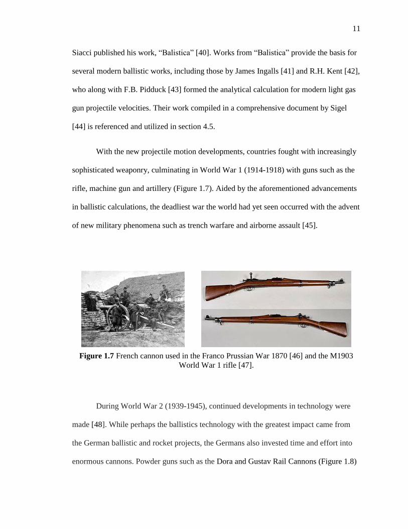
Figure 1.7 French cannon used in the Franco Prussian War 1870 [46] and the M1903
World War 1 rifle [47]. ............................................................................. 11
Figure 1.8 German rail cannons “Gustov” (top), “Dora” (left) [52] and V3 (right)
[53]. ........................................................................................................... 13
Figure 1.9 ENIAC and a pair of computer operators [55].......................................... 14
Figure 1.10 Progression of Hydrocodes [67]. .............................................................. 18
Figure 1.11 Rocket sled track at Sandia National Laboratories [68]. .......................... 19
Figure 1.12 Components of a typical single stage light gas gun [71]. ......................... 20
Figure 1.13 Typical components within a two stage light gas gun [73]. ..................... 21
Figure 1.14 Historical view of peak gas gun velocity over the years 1945-1995 [73]. 22
Figure 1.15 Nuclear stockpiles of the United States and Russia [74]. ......................... 23
Figure 1.16 Locations of a few academic and national gas gun facilities. ................... 25
Figure 1.17 Typical testing setups and testing methods [121]. .................................... 27
Figure 1.18 Projectile mass as a function of speed for three low mass accelerator types
[123]. ......................................................................................................... 28
Figure 1.19 Plot of mass vs. speed of some well-known gas guns [150]. .................... 29
Figure 1.20 Gas gun facilities visited by the author. .................................................... 31
Figure 1.21 The history of Marquette’s Shock Physics Laboratory, 2001-2017. ........ 34
Figure 1.22 Liquid filled steel cylinder fragmentation experiment [125]. ................... 35
Figure 1.23 Marquette’s original 1 inch single stage light gas gun. ............................ 36
Figure 1.24 P-v plot (above) of Hugoniot curves and P-t diagram (below) for a flyer
impacting a 0.1 g/cc silica sample at 405 m/s ........................................... 37
Figure 1.25 Stress, density, and Us Up relations for Al-MnO2-expoxy. ..................... 38
Figure 1.26 Lift in lbs experienced by a baseball traveling at 70 mph rotating at 50
rpm, red is indicative of behavior experienced by a knuckle ball. ........... 39
Figure 1.27 Pressure residuals taken from various equations of state for varying
specific volume. ........................................................................................ 40
Figure 1.28 Dynamically compacted aviation brake powder at 0.203 GPa. ................ 41
Figure 1.29 Comparison of shock pressure measured for 0.1g/cc porous silica at
1100 m/s. ................................................................................................... 42
Figure 1.30 Sensitivity analysis of water equation of state. ......................................... 43

vi
Figure 1.31 Progression of fracture within a single grain of sand. .............................. 44
Figure 1.32 Marquette’s 1/4 inch single stage light gas gun. ....................................... 45
Figure 1.33 Marquette Shock Physics Borg Collective.
(left to right): Emilie Teitz, Logan Beaver, Nathaniel Helminiak, Dr. John
Borg, Longhao Huang, Jeff LaJeunesse, Peter Sable and Janaka Kosgolla.
................................................................................................................... 45
Figure 1.34 Mysterious components within the Shock Physics Lab, and later
installation of completed design. .............................................................. 47
Figure 1.35 Two dimensional sections of temperature and stress paired with
distributions of temperature and stress experienced during the simulation
of airline break powder from an impact of 800m/s. .................................. 48
Figure 1.36 Particle velocity profiles and domain for 425-500 µm diameter sand
grains. ........................................................................................................ 49
Figure 1.37 Normalized view of experimental velocity data taken from PIV (data
clearly shows the shear effects near the projectile wall in addition to the
location of the compaction wave created by the projectile). A non-
dimensional plot of momentum diffusion with non-dimensional time
shows a linear relationship between momentum, diffusion and projectile
velocity. ..................................................................................................... 50
Figure 1.38 The kinetic energy output of an aluminum cylinder driven by an explosive
TNT charge as a function of outer radius and wall thickness. The materials
used were aluminum for the wall and TNT for the explosive. ................. 51
Figure 1.39 Experimental Setup and numerical simulations of shock waves through
water. ......................................................................................................... 52
Figure 1.40 Optical PDV setup with yellow collimators testing moving targets (spun
on the Dremel) and stationary targets such as the rectangular clamped
sample. ...................................................................................................... 53
Figure 2.1 Preliminary concept showcasing the gun system overview. ..................... 54
Figure 2.2 Discovery and removal of tailings. ........................................................... 56
Figure 2.3 Scanning electron microscope and sampled material composition. ......... 57
Figure 2.4 Fatigue strength of AISI 4135 steel [142]................................................. 58
Figure 2.5 Breach assembly and dimensions (taken by caliper). ............................... 58
Figure 2.6 Breach’s flat unstayed head configuration from ASME. .......................... 62
Figure 2.7 The breach assembly. ................................................................................ 65
Figure 2.8 5 ft. sections of the brass barrel cleaning brush. ....................................... 73
Figure 2.9 A sectioned sabot separating from a long rod penetrator [149]. ............... 74
Figure 2.10 Sabot dimensions. ..................................................................................... 75
Figure 2.11 Completed sabot design. ........................................................................... 76
Figure 2.12 Flange mating the barrel with the target tank. .......................................... 78
Figure 2.13 Target tank with external features and teardown of the bulkhead. ........... 82

vii
Figure 2.14 Vacuum re-pressurization valve. .............................................................. 83
Figure 2.15 Bulkhead, dimensions, and components. .................................................. 84
Figure 2.16 Dial indicator to align the target plate and a mounted sample. ................. 85
Figure 2.17 Sample mounted on the target plate. ......................................................... 86
Figure 2.18 Blast shield CAD model and completed design. ...................................... 87
Figure 2.19 The catch tank: attaching the vacuum mount plate. .................................. 89
Figure 2.20 Agilent vacuum pump mounting points. ................................................... 89
Figure 2.21 Impact plate. .............................................................................................. 90
Figure 2.22 Range of pressure loads experienced by the chains securing the catch tank
impact plate. .............................................................................................. 94
Figure 2.23 Early testing utilizing remote labview control station. ............................. 96
Figure 2.24 Main electrical control box. ...................................................................... 97
Figure 2.25 Single 10ksi distribution electrical system utilizing NI 9481 and 9205
modules. .................................................................................................... 99
Figure 2.26 Vacuum pump switch. ............................................................................ 100
Figure 2.27 Haskel power circuit operating the MAC solenoid. ................................ 101
Figure 2.28 National Instruments signal connection guide [153]. ............................. 102
Figure 2.29 Operator debug screen. ........................................................................... 103
Figure 2.30 Pictographic gun control display. ........................................................... 104
Figure 2.31 Pressure distribution control system. ...................................................... 105
Figure 2.32 Haskel, safety vacuum valve, and Agilent pump switch control. ........... 106
Figure 2.33 Signal data collection from the high and low pressure chambers as well as
vacuum pressure...................................................................................... 107
Figure 2.34 Legacy Haskel flow control diagram. ..................................................... 108
Figure 2.35 Conceptualized artistic rendition of the pressure booster’s interior
mechanism. ............................................................................................. 109
Figure 2.36 Pressurization system reference sheet. .................................................... 111
Figure 2.37 Completed pressurization system. .......................................................... 113
Figure 2.38 Distribution system reference sheet. ....................................................... 115
Figure 2.39 10ksi pressure distribution system for high and low side breach chambers.
................................................................................................................. 117
Figure 2.40 Three common types of firing mechanism. High pressure gas within the
breach can be seen in blue while evacuated volume is colored purple. .. 118
Figure 2.41 Dual diaphragm system firing sequence. ................................................ 120
Figure 2.42 Laser gate experimental setup. ................................................................ 121
Figure 2.43 Light gate dimensions. ............................................................................ 122
Figure 2.44 Light gate reading from a 390 psig, 0.4322 kg shot. .............................. 123
Figure 2.45 Photon Doppler Velocimetry and Dynasen pin system. ......................... 125
Figure 2.46 Red and blue shift in stars [158]. ............................................................ 126

viii
Figure 2.47 Sputter coating machines in Marquette’s Mechanical Engineering
Department (Technics Hummer 1) and Dental School (MTI GSL-1100x-
SPC-12) respectively. ............................................................................. 127
Figure 2.48 Sputtering rates for the Marquette Dental School sputter machine [159].
................................................................................................................. 128
Figure 2.49 Sputter coated acrylic sample. ................................................................ 129
Figure 2.50 Recommened surface profiles. ................................................................ 130
Figure 2.51 Down barrel PDV. .................................................................................. 131
Figure 2.52 Raw PDV output for the down barrel probe. .......................................... 131
Figure 2.53 Plots of identical datasets displaying FFT output. .................................. 132
Figure 2.54 Final data collected from the down barrel PDV. .................................... 134
Figure 2.55 Piezoelectric pin [160]. ........................................................................... 135
Figure 2.56 Conductive make-pin [160]. ................................................................... 135
Figure 2.57 The Marquette 2 inch gun vacuum system. ............................................ 136
Figure 2.58 Vacuum gauges: high pressure and low pressure. .................................. 138
Figure 2.59 Distribution system reference diagram. .................................................. 139
Figure 2.60 Marquette machine shop. ........................................................................ 142
Figure 2.61 Examples of available milling tools from left to right, chipped teeth,
clogged flutes, ideal tool. ........................................................................ 143
Figure 2.62 A myriad of tools are available to achieve higher precision machining.
gauge blocks (mill), dials (mill and lathe) and the wiggler (mill) are all
excellent tools to keep the dimensions of one’s part on point. ............... 144
Figure 2.63 Steel chips from left to right: blue, silver, and gold................................ 145
Figure 4.1 Performance curve for the AGT-62/152H Haskel Pressure Booster [165].
PS is the gas supply pressure (psig), Pa is the driving pressure (psig), Po is
the outlet pressure (psig), and QA is the gas flow of the outlet gas
(SCFM). .................................................................................................. 157
Figure 4.2 Pressurization curve of the combined small and large chamber volume
within the breach for different flow control valves to the Haskel drive air
supply. ..................................................................................................... 159
Figure 4.3 Burst disks in varying states of failure; note the bulging effect of the
bronze disk, which changes the internal volumes of both chambers. ..... 161
Figure 4.4 Examples of proper (left) and improper disk failure (right). .................. 162
Figure 4.5 Range of theoretical set pressures for a 0.125 Alum-Alum burst disk
configuration using nominal burst pressure. ........................................... 164
Figure 4.6 Plot for the effective working range of 0.125 inch Alum – 0.125 inch
Alum burst disk configuration including a 9 Ply Mylar – 0.125 inch Alum
burst disk configuration. ......................................................................... 167
Figure 4.7 Plot of burst pressure vs thickness ratio for various stainless steel 304 and
305 round burst disks. This where P is the burst pressure, E is the modulus

ix
of elasticity, t is the disk thickness, r is the diaphragm bend radius, a is the
radius of the unsupported disk area, d is the material left at the bottom of
the groove, 𝜎𝑢𝑙𝑡 is the ultimate strength of the diaphragm, 𝜎𝑎𝑢 is the
apparent strength of the diaphragm, 𝜖𝑢𝑙𝑡 is the ultimate strain, and 𝜖𝑎𝑢 is
the apparent ultimate strain. .................................................................... 170
Figure 4.8 Burst disk failure approximation. ........................................................... 171
Figure 4.9 Pressure vs. thickness for mylar with material characteristics. .............. 174
Figure 4.10 Post shot sabot profile, for a projectile shot at 600 psig. ........................ 176
Figure 4.11 Post shot sabot profile; sabot shot at 960 psig. ....................................... 178
Figure 4.12 Three vacuum flow regimes [175]. ......................................................... 181
Figure 4.13 Manufacturer pump curve with fitting [179]. ......................................... 184
Figure 4.14 Pressure and pumping speed within the system as a function of time. ... 185
Figure 4.15 Compressibility factors of nitrogen and helium [182]. ........................... 195
Figure 4.16 An x-t diagram of pressure waves emanating from the voids left by the
sabot [150]. ............................................................................................. 196
Figure 4.17 Approximate gas gun pressure velocity profile for a variety of models for
a 0.25 kg projectile. ................................................................................. 209
Figure 4.18 Non-dimensionalized pressure velocity curves with three observed tests.
................................................................................................................. 210
Figure 4.19 Estimation of sabot travel time (converged to 7.87 millisec) for a 0.25 kg
projectile with a breach pressure of 10,000 psig. .................................... 212
Figure 4.20 Final system pressures based on initial breach pressures. ...................... 214
Figure 5.1 Mating of two marble blocks [193]. ....................................................... 218
Figure 5.2 Diagram of the Harvard optical alignment method. ............................... 219
Figure 5.3 Optical alignment by use of the auto-collimating telescope [194]. ........ 220
Figure 5.4 Proposed method to employ the Brown method into the Marquette gas gun
design. ..................................................................................................... 221
Figure 5.5 A novel proposed method for the alignment of oblique impacts used in
pressure shear. ......................................................................................... 222
Figure 5.6 Samples cut by a metal cutting laser and triangular machining bit. ....... 222
Figure 5.7 Demonstration of the ROBONANO α-0iB, creating a retroreflective
surface. .................................................................................................... 223
Figure 5.8 Flyer plate impact of aluminum impacting copper at 600m/s. ............... 224
Figure 5.9 Three common types of shock physics experiments. .............................. 225
Figure 5.10 Transverse and longitudinal waves. ........................................................ 225
Figure 5.11 1-9-2017 test shot for the shock consolidation of powders. ................... 226
Figure 5.12 Completed 2 inch single stage dual diaphragm gas gun. ........................ 227

1
1. INTRODUCTION
1.1 Motivation
The objective of this work is three fold:
First, a usable platform is created from which to conduct shock experiments. The
current work platform includes 1D Planar Shock, Shock Compaction of Materials,
Pressure Shear, Granular Material Compaction and Conical Shots. However, the gun
capability could be adjusted to include work on penetration studies and damage
modeling.
Second, this work seeks to demonstrate the operational safety of the 2 inch gas
gun with a manual giving clear record of parts, their selection and operation. It is
expected that with time the gun will adapt and improve; however, the basics will likely
remain the same.
Third, it is desired to provide the new shock physics researcher with a suite of
tools with which to conduct research. By simplifying gun operation and optimizing
performance, more focus is placed on novel research. To this end, explicit scripts have
been included within this works’ appendices, which should allow the researcher to
quickly create operational parameters to suit experiments and ensure the 2 inch gas gun
will operate both correctly and consistently. Sections within this thesis should be
consulted as first reference for use of the Gas Gun, then if there are questions, feel free to
contact the author.

2
1.2 History and Review
1.2.1 Ballistics in History: A Path to Gas Gun Technology and Shock Physics
It is unknown when the human race first began experimenting with projectiles.
One would have to imagine it happened somewhat like this: Early humans through
observation or by happenstance did cause to effect or did witness a significant change in
the velocity of a local object apart from the effecter resulting in an impact a distance from
the point of origin. This use of projectiles was eventually utilized by an individual as a
tool/weapon and this tool was later passed to other individuals through history.
A selection of some of the projectile tools/weapons found earliest in human
history is compiled below in Figure 1.1. Though the exact use of some of the artifacts
complied is sometimes questioned as humans of that time left no clear messages or
recording of use [1], it is clear that developments in projectile technology were well
underway. Spears such the Schöningen spear [2] (378,000 and 398,000 BC) could be
utilized as both a short range and a long-range weapon. Bows and arrows found in
Kenya (9400 – 10500 BC) [3], improved mechanical advantage as well as creating an
ability to store potential energy in the form of string tension. Rock slings and stones
found in Turkey (7000 BC) [4] [5] increased the acceleration felt by projectiles through
use of longer moment arms.

3
Figure 1.1 Early ballistics technologies: spear [6], arrows [3], and slings [4].
From this point in history, others would improve upon the craft through various
methods of improving the peak velocity, accuracy and flight paths of these projectiles.
Continuing in time, one of the earliest known recording of projectile use is found on the
Stele of the Vultures (2500 – 2340 BC) found in modern day Iraq [7] where early man
recorded the usage of arrows in war (see Figure 1.2).
Figure 1.2 Stele of Vultures [8] and quote from the translation [9].

4
Stone and wooden tools became upgraded with stronger bronze enhancements.
The Bronze Age (3000 BC – 1000 BC) [10] tools were being used in more challenging
scenarios, hunting ever larger animals and using armor. With new challenges came a
continued demand for innovation and improvement. Metallurgical proficiency in the Iron
Age (1200 BC – 1200 AD) [11] would continue a trend searching for improvements
through material selection, which continues the present day. During the Iron Age, the
technologies of the spear sling and bow were enlarged. The Roman Mangonel (catapult)
is thought to have been developed around the same time 400 BC [12] in which the Greek
historian Diodorus Siculus documented the mechanical ballista as a weapon of war [13].
Just 100 years later in 300 BC the Chinese would develop the Trebuchet [13].
By this point, there was clear military and scholastic consideration undertaken by
people in history. Scientists such as Aristotle (364 – 322 BC) would begin to ponder the
nature of motion. Theories in his work, “Physics” [14], considered the natural motion of
materials to be governed by the amount of certain fundamental elements within an object:
earth, air, water, fire, and ether. Each object would attempt to move towards other
elements of certain types, which encircled the earth in layers: water surrounding earth, air
rising through water, and fire rising through air. When an object like a stone, which was
made of the earth element, was placed in water or flung through the air, it tended to seek
out its natural place falling through other elements attempting to reach its natural place on
the lowest plane of the elements. For projectile motion, an object would first use up
violent motion, traveling in a straight line and then follow natural motion, moving
directly to its natural place.

5
About this time, it is supposed that Archimedes of Syracuse (287 – 212 BC)
developed the first gas gun [15]. While the original work and perhaps publications of
Archimedes have not yet been found, his work on the “Architronito” [16] (see Figure
1.3), the first single stage light gas gun, was drawn by Leonardo da Vinci, who cited
Archimedes as its inventor. From notes, it appears that the system utilized steam to propel
targets at the enemy. It is likely that the cannon, while impressive for its time, took both a
long time to load as well as pressurize and was not yet practical for use on a moving
battlefield. Tests done by MIT showed that given optimal implementation of the design,
the “Architronito” was likely capable of firing a 0.5 kg projectile at a muzzle velocity of
280 m/s [17].

6
Figure 1.3 The “Architronito” drawn by Leonardo Da Vinci.
A solution to the problem of rapid power and quick loading would later be solved
by the Chinese between 948 and 951 AD [18]. An ancient Daoist text, the Zhenyuan
Miiaodao Yaolue, seems to refer to an ancient form of propellant. A military text
appearing a little later, Wujing Zongyao, gives careful instructions and recipe for gun

7
powder [19]. Historian Kenneth Chase points out evidence of primitive firearms in the
forms of fire lances, which could be loaded with small projectiles and expelled during
flaming. These are followed by cave temple painting in Sichuan dating from the 1100’s
AD, which include an early cannon and bomb. Hand canons, or early firearms, would
first appear in the Middle East battle of Ayn Jalut between the Egyptian Mamluks and the
Mongols, playing a part in stopping the Mongol goal of western expansion [20].
Firearm technology would be of great military importance as energy could be
stored in a form that was easy for the common man to apply, lowering the barriers of
strength and skill. From about 1100 AD onwards, the powdered gun would make its way
around the rest of Asia, Europe (see Figure 1.4), and Africa, where the firearm and
cannon would serve alongside the sword, spear, bow, horse, trebuchet, and catapult.
Indeed the historian Niccolo Machiavelli wrote in his 1519 The Art of War, “There is no
wall, whatever its thickness that artillery will not destroy in only a few days” [21].
Figure 1.4 The earliest pictogram found of a european cannon [22].

8
Eventually, the rifling of the barrel, invented by August Kotter in Germany during 1498,
would improve the accuracy of these projectiles [23]. Once projectiles could be propelled
in a manner that was repeatable, scholars returned to the problem of predicting projectile
motion. Most gun operators at this time would use Tartaglia’s 1537 mixed motion
projectile model, which presumed that objects would initially start with all violent motion
and decay in a mixed state to natural motion (explaining an object’s more curved
trajectory) [24]. Galileo’s theory of parabolic motion was first published in Speccio
Ustoria [25] by means of a former Jesuit student, Bonaventrua Cavaleri. Later, Galileo in
1636 would expound upon this theory in his own work, “Discourses Concerning Two
New Sciences” [26], stating that an object would fall with constant acceleration during its
travel to earth, meaning that a projectile’s motion was chiefly parabolic. Issac Newton in
1656 would add air resistance showing that drag at low velocities was proportional to the
density of the fluid through which the projectile travels, cross sectional area, and shot
weight [27]. Johann Bernoulli in 1695 would formulate, by assuming uniform density, a
relation between the pressure energy contributing to drag and the velocity of a projectile,
which is known today as the Bernoulli equation [28].
Manufacturers during this period also did a great deal to improve the firearms of
the day. Cannons that were scaled down in size could be carried in one’s hand; hence,
they were given the name “hand cannon”. These cannons were improved with the
addition of an ergonomic body and matchlock system, like the one seen in the French
Blunderbuss (handgun) shown in Figure 1.5. Finally, ball shot was replaced with a
conical bullet and spiral cut (rifled) barrel creating a rifle much akin to a modern weapon.

9
Figure 1.5 1760 French Blunderbuss [29] and a 1803 British Baker Rifle [30].
As manufacturing improved and guns reached a new plateau in terms of working
principle, scientists again began to make significant progress. Benjamin Robins invented
the ballistic pendulum, which allowed for the measurement of projectile and muzzle
velocities. In his 1805 book “New Principles of Gunnery” [31], Robins utilized the
principles of numerical integration by Euler [32] to determine projectile motion, which
Euler himself would later translate to German with added contributions.
Inspired by John Locke’s Electro-Chronograph created in 1848, with its ability to record
events in time [33], Francis Bashforth improved upon Robins’ method to measure
ballistic velocity with the creation of the Electro-ballistic ChronoGraph (Figure 1.6) [34].
With this electro-chronograph, Bashforth and others tested a variety of projectiles shapes,
angles, charge strength, and environmental conditions.

10
Figure 1.6 Francis Bashforth’s Electro-ballistic ChronoGraph [35].
Armed with increasingly accurate experimental data, numerical models of
calculating projectile motion also became quite accurate. Though these model methods
were very precise, calculations required a long time to work out and were only valid for
standard projectile shapes. Solutions needed to be quickly determined for a given set of
battlefield conditions, so ballistic tables were developed using both experimental and
analytical solutions to provide accuracy in hitting a target [36] [37]. Ballistic tables by
Bashforth were later adapted by Russian General Mayevski [38] with additional
experimental data collected by M. Krupp [39]. In 1880, Italian Colonel Francesco
11
Siacci published his work, “Balistica” [40]. Works from “Balistica” provide the basis for
several modern ballistic works, including those by James Ingalls [41] and R.H. Kent [42],
who along with F.B. Pidduck [43] formed the analytical calculation for modern light gas
gun projectile velocities. Their work compiled in a comprehensive document by Sigel
[44] is referenced and utilized in section 4.5.
With the new projectile motion developments, countries fought with increasingly
sophisticated weaponry, culminating in World War 1 (1914-1918) with guns such as the
rifle, machine gun and artillery (Figure 1.7). Aided by the aforementioned advancements
in ballistic calculations, the deadliest war the world had yet seen occurred with the advent
of new military phenomena such as trench warfare and airborne assault [45].
Figure 1.7 French cannon used in the Franco Prussian War 1870 [46] and the M1903
World War 1 rifle [47].
During World War 2 (1939-1945), continued developments in technology were
made [48]. While perhaps the ballistics technology with the greatest impact came from
the German ballistic and rocket projects, the Germans also invested time and effort into
enormous cannons. Powder guns such as the Dora and Gustav Rail Cannons (Figure 1.8)

12
launched projectiles of high mass, 4,800 kg-7,100 kg (10,600-15,700 pounds), up to 38-
48km (24-30 miles) away [49]. Multi-charge powder “accelerating-guns”, like the V3
(Figure 1.8) developed by Haskell, R. and Lyman, A.S. [50], attempted to increase the
range of the single stage powder gun. Experiments carried out at the Sandy Hook Proving
Ground by the U.S. Army Ordinance Department found a multistage 6-inch gun had the
ability to shoot a 69 kg (152 pounds) projectile a velocity of 548.9m/s (1801 feet/second),
which was comparable in ability to that of single barrel guns of this same period [51].

13
Figure 1.8 German rail cannons “Gustov” (top), “Dora” (left) [52] and V3 (right) [53].
In order to calculate the vast number of projectile path solutions during World
War 2, a number of men and predominantly women were employed as equivalent
computers to calculate ballistics trajectories. After the end of the second World War, the
United States would unveil their newest tool the ENIAC (Figure 1.9), the first turing-
complete programmable electronic computer used for ballistic calculations in 1945 [54].

14
Trajectories of the standard projectile, as well as projectile paths of non-standard types,
could be calculated in a fraction of the time.
Figure 1.9 ENIAC and a pair of computer operators [55].
From World War 2 onwards computers ran and still run the majority of ballistic
calculations as well as the design and simulation of projectile impacts. No longer would
designs for ballistics solely remain with guns. Modern designs for missiles, armor,
spacecraft, and satellites, speeding up to velocities of 73km/s (45 miles/second) [56], all
rely on shock physics and related fields for designs. To engineer projectiles suited for
operation at these speeds, numerical hydrocodes are the tool used for simulations and
shock guns (such as powder and gas) that provide valuable experimental data with which
to inform models.

15
The advent of German rockets and missiles traveling at 6.0 km/s and the new
capability of the computer marked a continuation of change in warfare and industry
towards faster capable vehicles carrying weapons, satellites and personnel [57]. From the
time the U.S. left World War 2 and entered the Cold War to the present day, tools for
testing the behavior of materials under these extreme conditions have been needed.
1.2.2 A Brief History of Shock Physics and Numerical Tools
While not the chief focus of this paper, a quick primer mention of shock physics
is required as light gas guns primarily function within the shock regime. Shock physics
and simulations of shock events are often informed by experimental data captured within
light gas gun experiments.
Shock Physics is the study of materials under explosive or impact loading
conditions. Typically, these materials interact at high speeds and strain rates that create a
shock through a material. Shocks are first proposed in a work by Euler, who suggested
the existence of a discontinuous function that changes value instantaneously without a
gradient [58]. Poisson would later take this idea and apply it to sound waves [59]. A
historical review of shock phenomenon becomes muddy at this point, but a good
summary of the enfolding events can be found within Manuel D Salas’ article, “The
curious events leading to the theory of shock waves” [60]; indeed, this work corroborated
much of the previous histories found. In short, Sir William Tomson, Lord Rayleigh, and
Sir George Stokes would then argue over the applicability of the derived equations of
mass and momentum, as they seemed in violation of the conservation of energy [61].

16
Though it was initially thought that these equations would violate conservation of energy,
Rankine would discover the adiabatic nature of shock waves, allowing for the
conservation of energy [62]. Hugoniot would then close the loop relating kinetic energy
to internal energy [63], leaving the shock physics community with three equations for the
conservation of: mass, momentum, and energy. These could be closed with a material
equation of state and, if applicable, a material strength model. Models predating
hydrocodes would use jump equations (1.1)-(1.4) [64] to model the interactions of wave
fronts moving through a given material:
ρ0Us = ρ(Us − Up) (1.1)
P − P0 = ρ0UsUp (1.2)
PUp =1
2ρ0UsUp
2 + ρ0Us(E − E0) (1.3)
Us = UpS + C0 (1.4)
where ρ is density, Us is the shock speed, Up is the particle speed, P is pressure, E is
internal energy, S is the Hugoniot slope and C0 is the material bulk sound speed. These
jump equations, while not able to capture the full behavior of the Navier-Stokes equation,
provide researchers a quick way to anticipate general wave behavior between material
interfaces, through a method known as impedance matching. For those interested in a

17
complete outline of hydrocode equations and computational methods the author
recommends M.L. Wilkins’ “Computer simulation of dynamic phenomena” [66].
Hydrocodes, which include the Navier-Stokes equation and closure models, give
engineers and scientists the tools needed to simulate shock physics events. Two major
methods of computing impacts and shock mechanics were methods based in Eularian
(named by Dirchlet) and Lagrangian (named by D’Alembert) grid based mechanics [65]
(see Figure 1.10). In Eularian mechanics, mass would move through a fixed set of cells,
which proved most useful for large deformation and mixed material mechanics, but
struggled with fracture and material boundaries. Lagrangian codes, while excellent for
defining material boundaries (as the cells were mapped to the material), required that
material be re-meshed. This was problematic in instances where material fractured into
small pieces computationally expensive to re-mesh each step. Both types of codes are still
available today with the most modern codes, such as CTH, using mixed Eularian-
Lagrangian models. Marquette University’s own KO 1D hydrocode is a formulation of
the Lagraingian HEMP Hydrocode [66].

18
Figure 1.10 Progression of Hydrocodes [67].
1.2.3 The Gas Gun
The development of the rocket engine traveling in the range of one to tens of
kilometers per second spurred the development of test platforms capable of reproducing
high velocity and high strain rate events within repeatable laboratory conditions. The
U.S. would become an international hub from which shock physics experimentation and

19
development stemmed. While experiments could be and were conducted using rocket
sled facilities like those shown in Figure 1.11, these experiments can be quite costly and
time-consuming to setup.
Figure 1.11 Rocket sled track at Sandia National Laboratories [68].
Conversely, gas guns are around the world are used for their consistency and ease
of use in testing penetrations and impacts, creating new material types and expanding our
knowledge of material properties at high strain rates. While a system level test like a
rocket sled impact might provide the behavior of an entire system, its accuracy is tied to
the many specific variables of the particular experiment. A gas gun provides a tool to
precisely measure the responses and material properties of individual components.
Compiling results of multiple gas gun shots enables simulation to better understand the
underlining phenomena of a full-scale test. In short, gas guns afford experimental studies
a platform providing relatively cheap, clean, reliable and repeatable studies, which can be
used as building blocks to understand more complex systems and behaviors. The first
fully operational, documented, single stage light gas gun was developed by Professor E.J.

20
Workman at New Mexico Institute of Mining and Technology in 1948. His proposal
outlines a method for launching projectiles above 2.75 km/s, the limit of powder gas guns
at the time [70]. In Figure 1.12 below, a generalized schematic of a single stage gas gun
is shown. During the development of light gas gun technology, several technological
discoveries were made, such as gas molecular size and temperature being found to have
an effect on peak projectile velocities in addition to the initial pressure of the gas and
mass of the projectile [69].
Figure 1.12 Components of a typical single stage light gas gun [71].
As is shown in the above figure, a single stage light gas gun consists of a breach
that contains pressurized gases, often nitrogen, helium or hydrogen. This use of “light”
gases (low molecular weight) provides an increase in gas gun performance. In general,
light gases, having higher sound speeds and lower molecular weight, boost projectiles to
higher speeds for a given breach pressurization. Once the breach pressure is released into
the barrel by means of a fast acting valve, wrap-around breach or diaphragm system, the

21
projectile (composed of a sabot and sample) is propelled down the barrel and collides
with a target or other experimental setup. Eventually, researchers would add a second
barrel [72], compressing the gas used as the propellant for another barrel and boosting
experimental velocities even higher.
Figure 1.13 Typical components within a two stage light gas gun [73].
In 1950, the initial work done by Professor Workman was classified and the gun
was lost to public research. Within the US government, work was continued at NASA
Ames and slowly spread to other branches of the government. Eventually light gas gun
development returned to public research institutions. Figure 1.14 below plots the progress
of velocities attained by light gas gun technology.

22
Figure 1.14 Historical view of peak gas gun velocity over the years 1945-1995 [73].
The 1970’s were a period of economic, and in turn research, struggle within the
United States. The period between 1970-1977, coined the gas gun “dark ages” by Hallock
Swift [73], saw reduction in research funding and a step backwards in progress. After the
recession, work was renewed in earnest. The shock community would receive renewed
initiative as the United States and Russia continued the Cold War, thus increasing the
importance of shock and nuclear physics as can be seen in Figure 1.15.

23
Figure 1.15 Nuclear stockpiles of the United States and Russia [74].
Support for the shock community would hit a new peak when the Reagan
administration began a new national program known as the Strategic Defense Initiative,
dubbed “Star Wars” by the public media of the time, which sought to intercept nuclear
warheads before impact with the United States [78]. Development of these light gas guns
was initially spearheaded by government, with scientific communities dedicated to the
field such as the Triservice Hypervelocity Impact Committee 1956 [73]. Others,
including the Aeroballistics Range Association (ARA) 1959 [75], HyperVelocity Impact
Society (HVIS) 1985 [76], and APS topical group, Shock Consolidation of Condensed
Matter (SCCM) [77], are still around today with vibrant communities.

24
From this point onward a variety of research institutions maintain over 50 gas
guns around the world, some of which are included and referenced in
Figure 1.16 below.
[80]
A: New Mexico Institute of Mining and Technology, New Mexico, USA, [79] [81]
B: Washington State University, Washington, USA, [82]
C: Ames Research Center, California, USA, [83]
D: Lawrence Livermore National Laboratory, California, USA, [84]
E: California Institute of Technology, California, USA, [85]
F: Los Alamos National Laboratory, New Mexico, USA, [86]
G: Shock Thermodynamics Applied Research (STAR) Facility, New Mexico, USA,
[87]
H: Oklahoma State University–Stillwater, Oklahoma, USA, [88]
I: Rice University, Texas, USA, [89]
J: Argonne National Lab, Illinois, USA, [90]
K: Marquette Shock Physics Laboritory, Wisconsin, USA, [71]
L: Arnold Engineering Development Complex, Tennesse, USA, [91]
M: University of Dayton, Ohio, USA, [92]
N: University of New Brunswick, New Brunswick, Canada, [93]
O: Harvard, Massachusetts USA Now University of California, Davis, California,
USA, [95]
P: Naval Ordnance Laboratory, Maryland, USA, [96]
Q: Naval Surface Weapons Center. Virginia, USA, [99]

25
R: Georgia Tech, Georgia, USA, [100]
S: Eglin Air Force Base, Florida, USA, [101]
T: Cavendish Laboratory, Cambridge, United Kingdom, [102], [103]
U: Imperial College, London, United Kingdom, [104]
V: University of Kent, Canterbury, United Kingdom, [105]
W: French-German Research Institute of Saint-Louis, Saint-Louis, France, [106]
X: Fraunhofer Institute for High-Speed Dynamics, Freiburg, Germany, [107]
Y: Zababakhin All-Russian Scientific Research Institute for Technical Physics,
Chelyabinck Oblast, Russia, [108]
Z: University of Tel-Aviv, Tel-Aviv, Israel, [109]
AA: Bhabha Atomic Research Center, Bombay, India, [110]
BB: China Academy of Space Technology (CAST), Beijing, China, [111]
CC: Japan Aerospace Exploration Agency (JAXA), Kanagawa, Japan, [112]
DD: Kyushu Institute of Technology, Kitakyushu, Japan, [113]
EE: Hypervelocity Impact Research Center, Mianyang, China, [114]
FF: Southwest Institute of Fluids Physics, Sichuan, China, [115]
GG: University of New South Wales, Sydney, Australia, [116]
HH: Materials Research Laboratory, DSTO Melbourne, Australia, [117]
II: DSTO Aeronautical and Maritime Research Laboratory, Salisbury South Australia,
Australia, [118]
Figure 1.16 Locations of a few academic and national gas gun facilities.
Within the shock physics community, there are generally three types of guns
utilized for projectiles of large mass (less than.1 kg), which are: powder guns, single
stage gas guns and two stage light gas guns. Velocities for these guns depend largely on
the mass of the projectile and the driving pressures; however, for the general scale
projectile (0.01 grams to 1000 grams), velocities and general uses are cited from Gun’s
Manufacturer Physics Applications Inc. [119].
Powder guns are most often the first facilities the uninitiated imagine when
thinking of shock physics gun research. In general, these facilities are harder to maintain
as the handling of explosives generally requires licensing. Residual powder and products
of the explosive reaction must also be cleaned after every experiment. Explosives, having

26
high energy concentration, are often the propellant of choice for the military, so these
guns serve to test behaviors of materials under similar loading conditions. Even though
explosives provide powder guns fast acceleration, they are not the fastest of the three
typical gun types, with powder guns typically operating between 0.3-2.7 km/s. Powder
guns are known for their use in armor penetration studies and testing of new projectile
shapes and materials. Single stage gas guns, like Marquette University’s, have a large
range of projectile velocities ranging from muzzle velocities less than 150 m/s to well
over 1000 km/s. These types of guns are used for equation of state research, high strain
rate testing of materials, creating new composite materials, testing the damage to air
planes from bird strikes and low velocity impact of space debris. Two stage gas guns test
in velocities in excess of powder or single stage gas guns. Space debris, ultra-high strain
rates, fusion reactions [120] and EOS testing as well as modern weaponry are all tested
with two stage gas guns. From this point, development may spread to even higher
velocities with three stage gas guns [92] or guns with multiple pressurized chamber
layers to overcome material strength limitations.
When thinking about gas guns it its useful to think in terms of strain rate. While
the civil engineers amongst the population work under the isothermal range of material
deformation, gas gun research moves far beyond the ranges of intermediate and high
strain rates. Gas guns approach ranges of material deformations where even solid
materials might instantaneously yield and flow in hydrodynamic fluid like flow.

27
Figure 1.17 Typical testing setups and testing methods [121].
Light gas guns are also used to test the largest of the small sized projectiles. For
small projectiles, light gas guns generally can produce experiments of meterorite and
micro meterorite impact. Perfromance at even lower mass is often completed by plasma
and electrostatic accelerators (Figure 1.18). With lower projectile mass projectile, speed
can be increased, with the smallest of projectiles on the order of atoms in size being
accelerated to over 99% the speed of light (296,794,533 m/s or 663,910,463 mph) at
CERN [122]

28
Figure 1.18 Projectile mass as a function of speed for three low mass accelerator types
[123].
A plot comparing the muzzle velocities of some well-known gas gun facilities
shooting projectiles at or above mesoscale is shown in Figure 1.19 below.

29
Figure 1.19 Plot of mass vs. speed of some well-known gas guns [150].
30
During the course of this research, this author had several opportunities to visit a
variety of shock physics facilities both in the United States and abroad as shown below in
Figure 1.20. While each facility functions using the same core principles guns are
customized to suit experiment: using slotted barrels to maintain the aliment of the sabot
with a target, manufacturing target tanks with additional hardware for using in cooling a
sample, or the addition of new diagnostic equipment such as a high speed pyrometer. The
author again wishes to thank the owners of these facilities, in which he was allowed to
absorb knowledge offered freely by these research groups. Facilities visited included
Harvard’s single stage gas gun facility, which is now moving to UC Davis. This research
group, headed by Sarah Stewart, researches geophysics and is well known for their
research into the phases of water. STAR is a US Department of Energy facility at Sandia
National Laboratories with several types of gas and powder guns. Their research covers a
wide variety of studies ranging from defense to research. Georgia Tech’s Facility does
similar work to Marquette with a single stage light gas gun research in flyer plate
experiments and granular material interactions. Finally, the University of Kent has a
small two stage gas and powder gun, with a shotgun cartridge providing the first stage
with power and compressed gas propelling the projectile. Kent utilizes their gas gun to
model astrophysics events including their most recent publication on the viability of
organisms reentering earth’s atmosphere.

31
Harvard [95]
Shock Thermodynamics Applied Research [87]
Georgia Tech [100]
University of Kent [105]
Figure 1.20 Gas gun facilities visited by the author.
This literature review is by no means comprehensive, though it does provide a
good overview of gas gun history and prehistory. For those seeking more detail, both
A.C. Charters “Development of the high-velocity gas-dynamics gun,” [124] as well as H.
F. Swifts “Light-Gas Gun Technology: A Historical Perspective” [73] are recommended.

32
After viewing other sources, these two articles admirably highlight historically relevant
events, from a perspective closer to the field in detail greater than in the text above.
1.2.4 Marquette’s History of Shock and Gas Guns
Marquette’s Shock facility has a long-standing pedigree stemming from its
inception with Dr. John Borg. By this time already, it seemed to the author that there was
a fair bit of history developed. While this history is partially outside of the scope of this
paper, it helps to both contextualize and provide reasoning for the newest gas gun’s
construction. It also provides a future historian with names, research developments and
reasons to include Marquette University as an institute of interest within the field of
shock research. The author apologizes in advanced for any missing or misinterpreted
information, specifically with regards to past researchers in the years before 2015, as the
researcher was involved in middle school to undergraduate academic teaching exercises
during this period. For those that wish to skip the brief summary of past Marquette Shock
Physics Research that follows a timeline is presented below in Figure 1.21.

33

34
Figure 1.21 The history of Marquette’s Shock Physics Laboratory, 2001-2017.
Marquette’s shock physics history begins with Dr. John Borg; a doctorate, full
professor and recent Mechanical Engineering Department Chair with initial academic
background in the areas of Fluids and Turbulence. From here Dr. Borg would become
lead engineer at the Naval Surface Warfare Center Computational Physics Group (1997-
2002) with shock physics related projects, including work involving the experimental
fracture of steel liquid filled cans (shown in Figure 1.22 below).
35
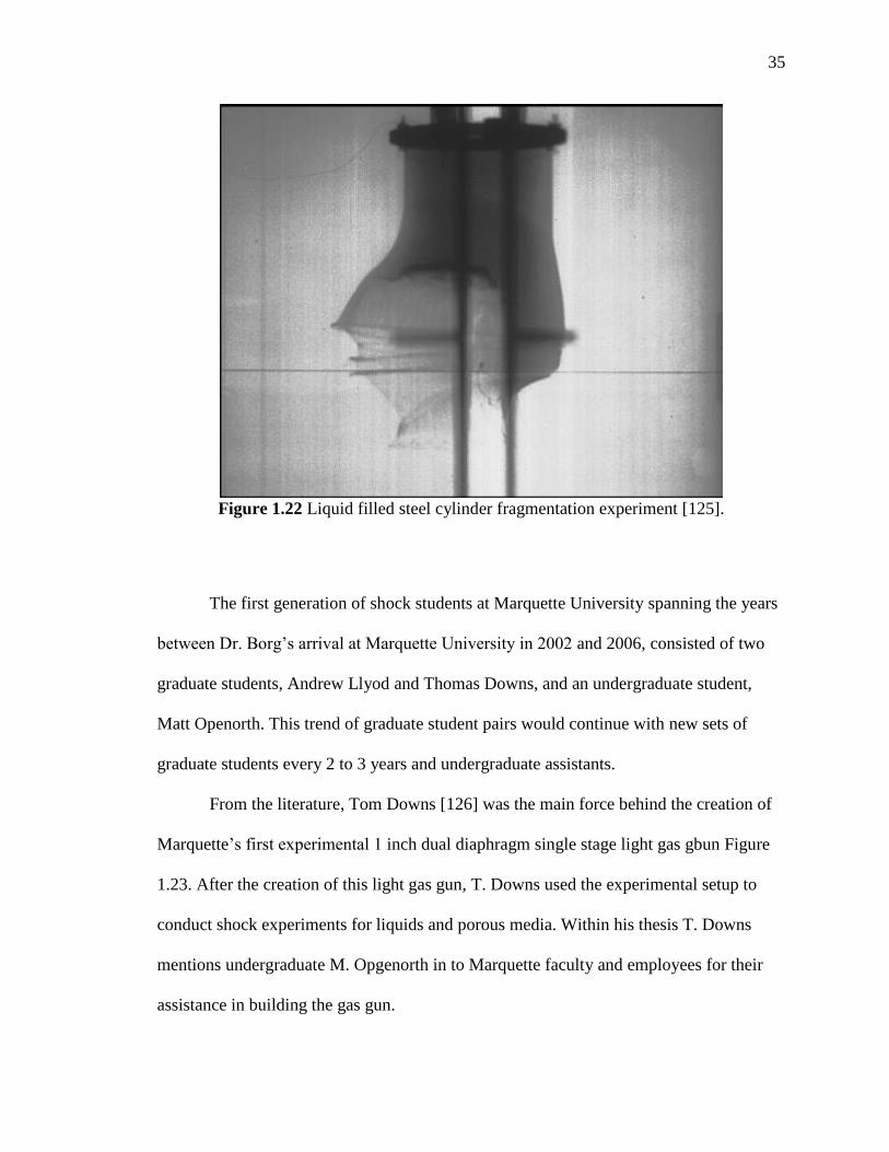
Figure 1.22 Liquid filled steel cylinder fragmentation experiment [125].
The first generation of shock students at Marquette University spanning the years
between Dr. Borg’s arrival at Marquette University in 2002 and 2006, consisted of two
graduate students, Andrew Llyod and Thomas Downs, and an undergraduate student,
Matt Openorth. This trend of graduate student pairs would continue with new sets of
graduate students every 2 to 3 years and undergraduate assistants.
From the literature, Tom Downs [126] was the main force behind the creation of
Marquette’s first experimental 1 inch dual diaphragm single stage light gas gbun Figure
1.23. After the creation of this light gas gun, T. Downs used the experimental setup to
conduct shock experiments for liquids and porous media. Within his thesis T. Downs
mentions undergraduate M. Opgenorth in to Marquette faculty and employees for their
assistance in building the gas gun.

36
Figure 1.23 Marquette’s original 1 inch single stage light gas gun.
During this same period, Andrew Llyod [127] would begin the use of CTH as
well KO hydro-codes, still in use by the Marquette physics lab, comparing the numerical
compaction of silica powder within CTH and KO against experimental data obtained at
Marquette Figure 1.24.
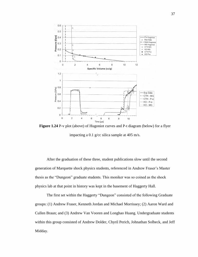
37
Figure 1.24 P-v plot (above) of Hugoniot curves and P-t diagram (below) for a flyer
impacting a 0.1 g/cc silica sample at 405 m/s.
After the graduation of these three, student publications slow until the second
generation of Marquette shock physics students, referenced in Andrew Fraser’s Master
thesis as the “Dungeon” graduate students. This moniker was so coined as the shock
physics lab at that point in history was kept in the basement of Haggerty Hall.
The first set within the Haggerty “Dungeon” consisted of the following Graduate
groups: (1) Andrew Fraser, Kenneth Jordan and Michael Morrissey; (2) Aaron Ward and
Cullen Braun; and (3) Andrew Van Vooren and Longhao Huang. Undergraduate students
within this group consisted of Andrew Dolder, Chyril Perich, Johnathan Solbeck, and Jeff
Midday.

38
Beginning with Andrew Fraser [128], research was conducted on shock
compaction of multiple component mixtures with numerical simulations of Al-MnO2-
Expoxy, shown in Figure 1.25, matching well with experiments conducted at the NSWC-
Indian Head 4in Gun Range. Amongst those mentioned in his thesis, A. Ward thanks Jeff
Midday and Michael Morrissey.
Figure 1.25 Stress, density, and Us Up relations for Al-MnO2-expoxy.
Michael Morrissey’s [129] thesis, not on shock, but rather the aerodynamics of
the knuckleball (Figure 1.26), showcased how the seams and initial throwing conditions
affect the evolution of ball trajectory and behavior, which brought much recognition to
the Mechanical Engineering Department. While not playing baseball, M. Morrissey also
conducted work on waveforms within Ottowa sand with graduate Andrew Fraser and
undergraduate Chyril Perich. Within his acknowledgements M. Morrissey thanks fellow
graduate student Aaron Ward as well as undergraduate Andrew Dolder.
39
`
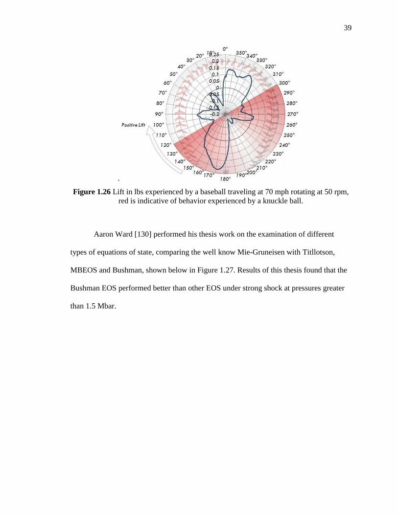
Figure 1.26 Lift in lbs experienced by a baseball traveling at 70 mph rotating at 50 rpm,
red is indicative of behavior experienced by a knuckle ball.
Aaron Ward [130] performed his thesis work on the examination of different
types of equations of state, comparing the well know Mie-Gruneisen with Titllotson,
MBEOS and Bushman, shown below in Figure 1.27. Results of this thesis found that the
Bushman EOS performed better than other EOS under strong shock at pressures greater
than 1.5 Mbar.

40
Figure 1.27 Pressure residuals taken from various equations of state for varying specific
volume.
Cullen Braun [131] researched the rapid compression of heterogeneous granular
mixtures for use in aviation brake pads (below in Figure 1.28). From his work with the 1
inch single stage gas gun, he was able to develop an equation of state and bulk sound
speeds for this specific material. Cullen Braun mentions Andrew Fraser and Ken Jordan
as helpful fellow graduate students.

41
Figure 1.28 Dynamically compacted aviation brake powder at 0.203 GPa.
Kenneth Jordan’s thesis [132] developed Marquette’s one dimensional hydrocode
KO based on Wilkins One Dimensional HEMP Formulation [66]. His work successfully
simulated shock wave with an irreversibility model, shown in Figure 1.29, rather than
artificial viscosity, reducing numerical error with the Mie-Gruneisen Equation of State.

42
Figure 1.29 Comparison of shock pressure measured for 0.1g/cc porous silica at
1100 m/s.
Longhao Huang’s research [134] focused on numerically simulating the
irreversibility of shock waves within gases and water focusing on the Mie-Gruneisen
Equation of State. In addition to parameter evaluation of water, his work also found that
the shock wave thickness did not seem to be a function of specific heat, heat
conductivity, viscosity nor length scale (see Figure 1.30). Longhao decided to continue
past his Masters and still continues towards his PhD.

43
Figure 1.30 Sensitivity analysis of water equation of state.
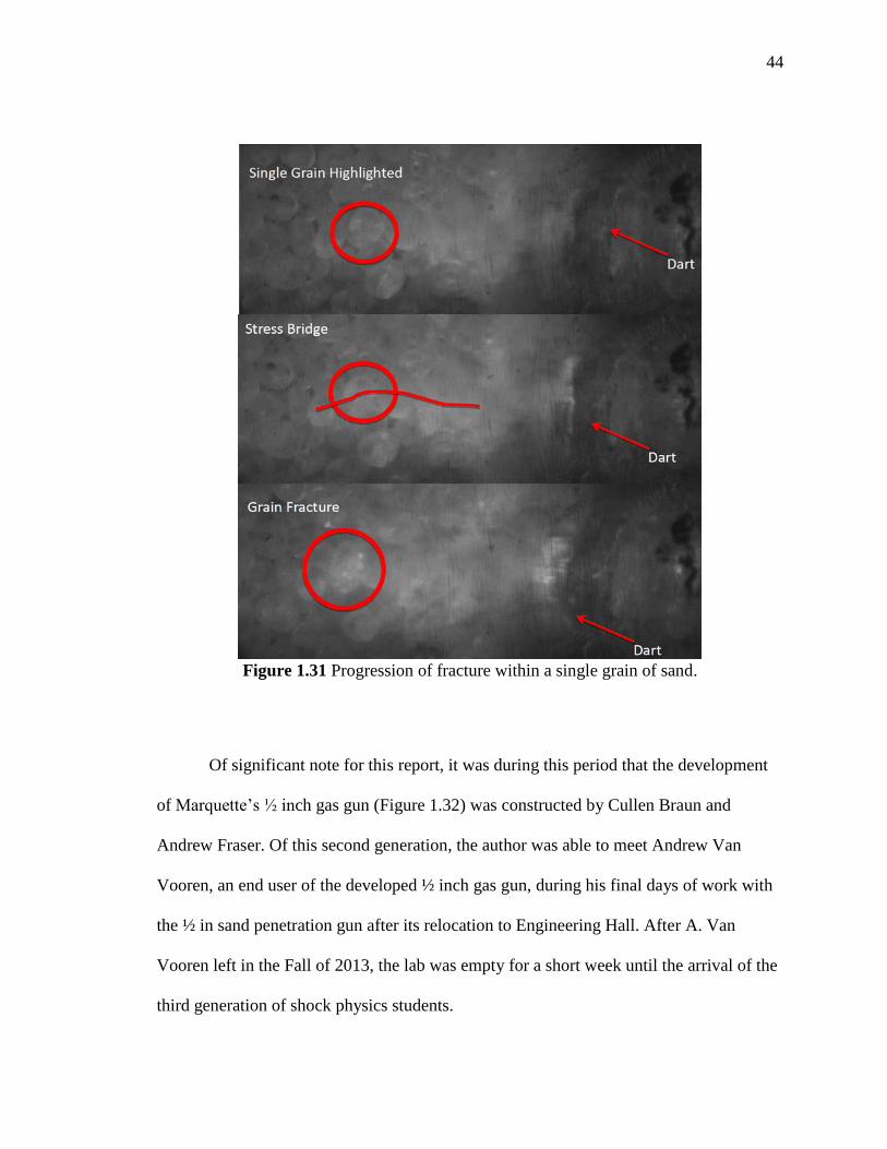
Finally Andrew Van Vooren [133] researched the behavior of heterogeneous
materials under dynamic loading, dart penetration into sand, both experimentally with
Marquette’s ½ in gas gun and numerically within EMU peridynamics. His results found
longitudinal and shear wave sound speeds as 263 m/s and 209 m/s respectively and
improved penetration with conical and hemispherical dart tips.
44
Figure 1.31 Progression of fracture within a single grain of sand.
Of significant note for this report, it was during this period that the development
of Marquette’s ½ inch gas gun (Figure 1.32) was constructed by Cullen Braun and
Andrew Fraser. Of this second generation, the author was able to meet Andrew Van
Vooren, an end user of the developed ½ inch gas gun, during his final days of work with
the ½ in sand penetration gun after its relocation to Engineering Hall. After A. Van
Vooren left in the Fall of 2013, the lab was empty for a short week until the arrival of the
third generation of shock physics students.

45
Figure 1.32 Marquette’s 1/4 inch single stage light gas gun.
This latest group, of which the author considers himself a part, consists of the
following individuals known as the Borg Collective (shown in Figure 1.33 below).
Figure 1.33 Marquette Shock Physics Borg Collective.
(left to right): Emilie Teitz, Logan Beaver, Nathaniel Helminiak, Dr. John Borg, Longhao
Huang, Jeff LaJeunesse, Peter Sable and Janaka Kosgolla.

46
The convention of naming labs seems to have grown either from the original
Haggerty Dungeon Dwellers or the ever-present Wede Lab run by Dr. Philip
Voglewede’s Dynamics Group (designated by a dandelion). On this brief tangent, the
Borg Collective has noticed other named laboratories appearing at Marquette: the Allen
Wrench Engine Research lab (also sometimes referred to as the tadpoles) run by Dr.
Casey Allen, and the Singer Nation run By Dr. Simcha Singer, which simulates particle
combustion. Perhaps this is a trend will continue…?
Returning to the current generation, new groups of graduate students (Jeffery
LaJeunesse, Merit Schumaker, Peter Sable, Nathaniel Helminiak, Logan Beaver, Emilie
Teitz and Christopher Johnson with undergraduates Trent Wolf and Ashley Hatzenbihler)
continue at present from prior group efforts. Janaka Kosgolla, shown in Figure 1.33, was
a post-doctoral student, who work closely with Dr. Borg and would frequently interact as
a coworker and friend.
Both Merit Schumaker and Jeffery LaJeunesse worked closely together on the
shock wave propagation within heterogeneous materials and together built the lab’s 64
core workstation “Thinkmate” presumably named after the company supplying the
hardware. The undergraduates, Trent Wolf and Nathaniel Helminiak, during the summer
of 2013, worked on parts of the ½ in gas gun and would observe and organize some
mysterious objects taking up space within the shock physics lab (Figure 1.34). The author
obviously decided to become a graduate student and continue work on those mysterious
objects.

47
Figure 1.34 Mysterious components within the Shock Physics Lab, and later installation
of completed design.
Merit Schumaker’s thesis [136] focused on the numerical simulation of
heterogeneous brake pad media undergoing dynamic compaction within CTH. By use of
this numeric technique, one could examine grain interaction (shown in Figure 1.35) in a
way which could not otherwise be seen with current experimental measurement methods.
Noted was CTH’s model of internal energy not directly capturing frictional heat and
irreversibility.

48
Figure 1.35 Two dimensional sections of temperature and stress paired with distributions
of temperature and stress experienced during the simulation of airline break powder from
an impact of 800m/s.
Jeffery LaJeunesse [135] in his thesis conducted similar work modeling velocity
profiles of shocks within sand of various grain diameters. Within his work, findings
indicated that a single simulation over a small sampling of experimental domain might
roughly capture the shock rise and steady state behavior on the rear of a sample. Of
importance, as shown in Figure 1.36, was a need to examine and average the behavior of
multiple tracers within the simulation for bulk behavior.

49
Figure 1.36 Particle velocity profiles and domain for 425-500 µm diameter sand grains.
Joining M. Schumaker and J. LaJeunesse one year later, Peter Sable [137]
finished work on sand penetration with Marquette’s ½ inch gas gun. His work, shown in
Figure 1.37 below, utilized a digital image correlation (DIC) technique to better
characterize sand interation with a kinetic pentrator. Through this, a better understanding
was of the mechanisms by which the kinetic energy of the projectile transferred
irreversibly into heat, grain motion, compaction and grain fracture. In addition, the
diffusion of momentum was found to have a positive relation with projectile velocity.

50
Figure 1.37 Normalized view of experimental velocity data taken from PIV (data clearly
shows the shear effects near the projectile wall in addition to the location of the
compaction wave created by the projectile). A non-dimensional plot of momentum
diffusion with non-dimensional time shows a linear relationship between momentum,
diffusion and projectile velocity.
Of these last three graduate students, both J. LaJeunesse and P. Sable decided to
continue their research at Marquette University as PhD students where they continued
work on shock compaction, pressure shear numerical simulations within CTH and
experimental data capture.
51
Logan Beaver [138] worked on two major projects. While his initial project
experimented with peridynamic simulation of granular mechanics, this study was
eventually shelved in favor of explosive simulations. His work utilized Marquette’s KO
model alongside CTH to model the effects of changing the ratio between explosive’s
radius and liner radius within exploding cylinders (see Figure 1.38). In addition, this
work compared the computational results of several parametric optimization studies
comparing genetic, gradient descent, and dividing rectangles algorithms.
Figure 1.38 The kinetic energy output of an aluminum cylinder driven by an explosive
TNT charge as a function of outer radius and wall thickness. The materials used were
aluminum for the wall and TNT for the explosive.
Emilie Teitz [139] worked as a one year master’s student and conducted shock
experiments within water shown in Figure 1.39. Her work continued to utilize the ½ inch

52
gas gun and tested some of the new remote firing systems added to the gas gun for
increased researcher safety.
Figure 1.39 Experimental Setup and numerical simulations of shock waves through
water.
Christopher Johnson, the most recent member of the Marquette Shock physics
community has continued development of the PDV System. His stationary work and that
using a rotating Dremel wheel has given the group added confidence that the PDV system
can accurately resolve the normal and transverse surface velocity components. The
experimental setup is presented in Figure 1.40 below. Developments from this work will
include the best material surface treatment and best practices to resolve velocity
components from pressure shear experiments.
53
Figure 1.40 Optical PDV setup with yellow collimators testing moving targets (spun on
the Dremel) and stationary targets such as the rectangular clamped sample.
The author would like to take this opportunity to thank the members of the Shock
Physics Group and other members of the community for laying a foundation upon which
this researcher could build and contribute. The review above is by no means
comprehensive but it is hoped that a concise history of the field might push readers to
explore more sections of history in depth. Thus ends the historical review of shock
physics research and gas gun history presented by this researcher. Topics appearing
within the text include references to other related fields relevant to the section in which
they reside.

54
2. CONSTRUCTION
This section comprises the design aspect behind Marquette’s new 2 inch dual
diaphragm single stage gas gun shown below in Figure 2.1. Designed to run on either a
cylinder of nitrogen or building supplied pressurized air, this system is meant to be a long
term experimental test bed for use by future shock researchers at Marquette University.
Care has been taken to ensure that safety of researchers is maintained through the
preparation and firing process in both construction, covered here, and policy, covered
later. This section attempts to both verify the safety of the gun from a design standpoint
as well as provide a complete listing of components necessary for replacement and day to
day operations. This will not cover specific diagnostic equipment such as particular
oscilloscope and only a brief overview of systems such as the PDV or Dynasen pin setup
which are out of the scope of this paper. Suggested resources for this information include
papers written by previous member of the Marquette shock physics community, which
are referenced in the previous historical section 1.2.4.
Figure 2.1 Preliminary concept showcasing the gun system overview.
55
2.1 Static Gun Components
2.1.1 Breach
The Marquette gas gun begins with an air source, supplied by either the 120 psig
building line or a 3,000 psig nitrogen tank from Airgas. Utilizing a Haskel pneumatic
piston compressor, the pressurization system can charge the breach and trigger cavity up
to the operational pressure of 10 ksi. Flow into and out of the breach and burst disk cavity
is remotely controlled by a set of four independently actuated valves, while a safety valve
ensures that the system remains at safe operating pressure. These will be covered in
greater depth in the active systems section.
The breach of the gas gun is the storage reservoir where the system’s future
kinetic energy reserves are stored as potential energy in the form of a pressurized gas.
While the breach can be thought of in loose terms as a gas tank, it is important to note
that it also serves as the structure of the dual diaphragm launch system, allowing for the
placement of burst disks within the breach assembly.
Upon receiving the breach and barrel assembly from Physics Applications Inc.
both the barrel and breach were rinsed in oil and tailings from the manufacturing process
were recovered in large quantity from both breach and barrel which were used to identify
the material utilized.

56
Figure 2.2 Discovery and removal of tailings.
While the tailings were too small to test in a hardness tester, the availability of
Marquette’s Scanning Electron Microscope allowed for an elemental breakdown of the
metal. The metal based on the presences of both Chromium and Molybdenum (shown in
Figure 2.3 below) in addition to Magnesium, Iron, and Carbon, fit the composition of the
41xx series of steel [140]. Reviewing the metal compositions, it is assumed that both the
barrel and breach were formed from 4135 or 4140 Steel commonly referred to as
ordnance or gun steel [141].

57
Figure 2.3 Scanning electron microscope and sampled material composition.
In order to verify the ability of the received breach and assess the pressurization
safety factor, CES Edupack’s data on AISI 4135 Steel (The lower carbon conservative
estimate) was utilized summarized below in Table 2.1 and Figure 2.4.
Table 2.1 Mechanical Properties of AISI 4135 Steel [142]
Mechanical Properties Value Units
Young’s Modulus 29-30.5 10^6 psi
Yield Strength 70.1-85 ksi
Tensile Strength 90.1-100 ksi
58
Figure 2.4 Fatigue strength of AISI 4135 steel [142].
Having identified the breach material, one can now verify the engineering and
safety of the delivered parts. In order to evaluate the safety of the breach it is necessary to
examine both the shell and cap head. Breach dimensions are given below in Figure 2.5.
Figure 2.5 Breach assembly and dimensions (taken by caliper).
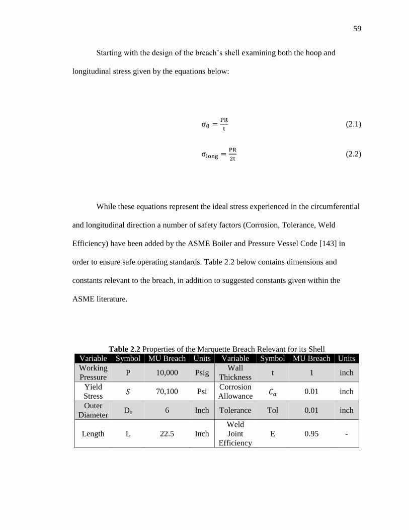
59
Starting with the design of the breach’s shell examining both the hoop and
longitudinal stress given by the equations below:
σθ =PR
t (2.1)
σlong =PR
2t (2.2)
While these equations represent the ideal stress experienced in the circumferential
and longitudinal direction a number of safety factors (Corrosion, Tolerance, Weld
Efficiency) have been added by the ASME Boiler and Pressure Vessel Code [143] in
order to ensure safe operating standards. Table 2.2 below contains dimensions and
constants relevant to the breach, in addition to suggested constants given within the
ASME literature.
Table 2.2 Properties of the Marquette Breach Relevant for its Shell
Variable Symbol MU Breach Units Variable Symbol MU Breach Units
Working
Pressure P 10,000 Psig
Wall
Thickness t 1 inch
Yield
Stress 𝑆 70,100 Psi
Corrosion
Allowance 𝐶𝑎 0.01 inch
Outer
Diameter Do 6 Inch Tolerance Tol 0.01 inch
Length L 22.5 Inch
Weld
Joint
Efficiency
E 0.95 -
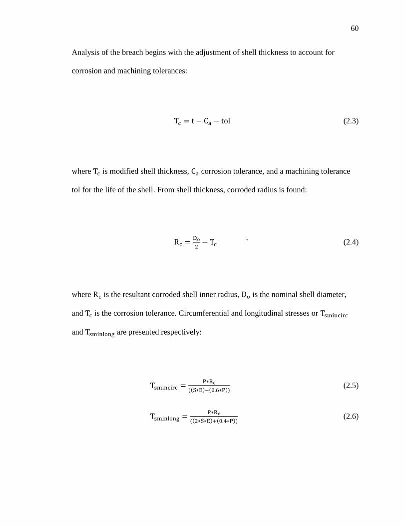
60
Analysis of the breach begins with the adjustment of shell thickness to account for
corrosion and machining tolerances:
Tc = t − Ca − tol (2.3)
where Tc is modified shell thickness, Ca corrosion tolerance, and a machining tolerance
tol for the life of the shell. From shell thickness, corroded radius is found:
Rc =Do
2− Tc ` (2.4)
where Rc is the resultant corroded shell inner radius, Do is the nominal shell diameter,
and Tc is the corrosion tolerance. Circumferential and longitudinal stresses or Tsmincirc
and Tsminlong are presented respectively:
Tsmincirc =P∗Rc
((S∗E)−(0.6∗P)) (2.5)
Tsminlong =P∗Rc
((2∗S∗E)+(0.4∗P)) (2.6)

61
which calculate minimum acceptable shell thicknesses based on the working pressure P,
corroded shell inner radius Rc, Material Strength S, and weld joint efficiency E. From
these stresses maximum internal pressures Pmaxcirc and Pmaxlong are found:
Pmaxcirc =S∗E∗Tc
(Rc+0.6∗Tc) (2.7)
Pmaxlong =2∗S∗E∗Tc
(Rc−0.4∗Tc) (2.8)
In calculating, it was found that the circumferential shear stress (hoop direction)
controlled the equation giving a maximum system pressure (before material deformation
or yield) of 25 ksi. This was 2.5 times greater (for a safety factor of 2.5) than the
maximum working pressure. Records of variables above and computed values are
summarized in Table 2.3 below.
Table 2.3 Computed Properties of the Marquette Breach Relevant for its Shell
Variable Symbol Value Units Variable Symbol Value Units
Corroded Shell
Thickness 𝑇𝑐 0.98 Inch
Yield Pressure
(Circumferential) 𝑃𝑠𝑚𝑎𝑥𝑐𝑖𝑟𝑐 25 ksi
Corroded Internal
Radius 𝑅𝑐 2.02 Inch
Yield Pressure
(Longitudinal) 𝑃𝑠𝑚𝑎𝑥𝑙𝑜𝑛𝑔 80 ksi
Minimum Shell
Thickness
(Circumferential) 𝑇𝑠𝑚𝑖𝑛𝑐𝑖𝑟𝑐 0.333 Inch
Approximated
Enclosed Volume V ~ 4.72 liters
Minimum Shell
Thickness
(Longitudinal)
𝑇𝑠𝑚𝑖𝑛𝑙𝑜𝑛𝑔 0.147 Inch Designed
Enclosed Volume V 4.5 liters

62
As an additional aside, the lifecycle graph (Figure 2.4) shows that at upwards of
1e8 cycles (Approximately 0.25 million years of firing, assuming a shot a day) the breach
should still be able to withstand 14,279 psig, well over the peak operating pressure. It is
with confidence that the breach will last longer than the lab given current designed usage.
Continuing, attention is turned to the breach’s single unstayed head (as the other
is capped by burst disks). “Unstayed” in this case refers to the idea that the head is
attached to the cylindrical shell on its own and resists internal pressures without the aid of
screws or braces attached on an external assembly. In this case, qualitative assessment,
while viewing the internals of the unwelded tank head, matched closest with the b-2
unstayed head type shown for reference in Figure 2.6.
Figure 2.6 Breach’s flat unstayed head configuration from ASME.
As before equations are taken from the ASME Pressure code. C below represents the
typical unstayed head connection factor:
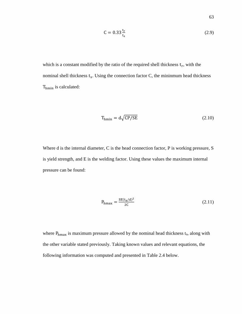
63
C = 0.33tr
ts (2.9)
which is a constant modified by the ratio of the required shell thickness tr, with the
nominal shell thickness ts. Using the connection factor C, the mininmum head thickness
Thmin is calculated:
Thmin = d√CP/SE (2.10)
Where d is the internal diameter, C is the head connection factor, P is working pressure, S
is yield strength, and E is the welding factor. Using these values the maximum internal
pressure can be found:
Phmax =SE(ta/d)2
2C (2.11)
where Phmax is maximum pressure allowed by the nominal head thickness ta, along with
the other variable stated previously. Taking known values and relevant equations, the
following information was computed and presented in Table 2.4 below.

64
Table 2.4 Computed Properties of the Marquette Breach Relevant for its Head
Variable Symbol MU
Breach Units Variable Symbol
MU
Breach Units
Nominal
Shell
Thickness 𝑡𝑠 1 inch
Design
Pressure P 10,000 psig
Required
Shell
Thickness 𝑡𝑟 0.353 inch
Actual
Head
Thickness 𝑡𝑎 2 inch
Internal
Diameter D 4 inch
Welding
Factor 𝐸 .95 -
Head
Connection
Factor
C
Unwelded
UG-34
Type b-2
-
Minimum
Head
Thickness 𝑇ℎ𝑚𝑖𝑛 0.529 inch
Allowable
Stress S 70,100 Psi
Maximum
Head
Pressure 𝑃ℎ𝑚𝑎𝑥 142,920 psig
Reviewing values, it is clear that the unstayed head is sufficient to the task of
holding back pressures well in excess of working pressures. While the breach will only
be pressurized to 10,000 psig, the breach head is capable of withstanding 142,920 psig, a
safety factor over 10.
Finally, the breach can be both open and closed via a collar assembly, which is
fastened via custom threading Figure 2.7. In the collar assembly there is a set of two
threaded sections. The smaller threaded section of the barrel is attached to an inner collar
piece, which is surrounded by a free sliding outer collar. The sliding outer collar is then
attached to the breach by a second set of threads. As the location of the inner collar can
be set independently to wide variety of distances along the barrel, knowing the minimum
allowable engaged thread length of both the inner and outer collar was of high
importance.
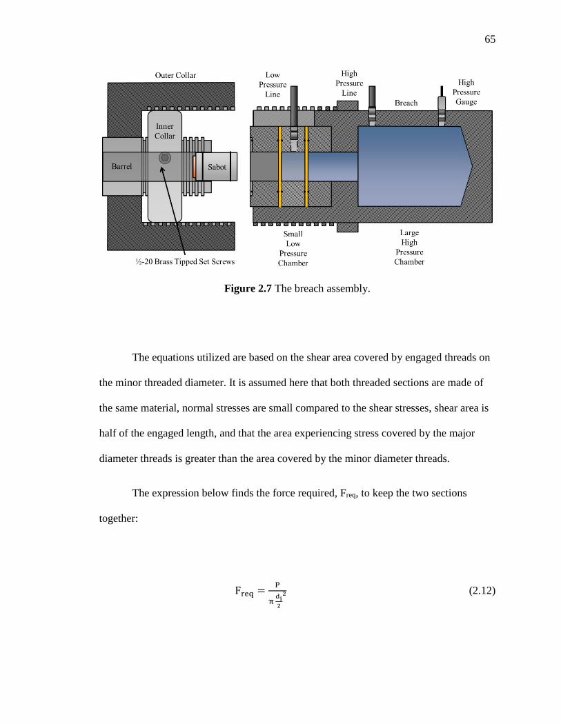
65
Figure 2.7 The breach assembly.
The equations utilized are based on the shear area covered by engaged threads on
the minor threaded diameter. It is assumed here that both threaded sections are made of
the same material, normal stresses are small compared to the shear stresses, shear area is
half of the engaged length, and that the area experiencing stress covered by the major
diameter threads is greater than the area covered by the minor diameter threads.
The expression below finds the force required, Freq, to keep the two sections
together:
Freq =P
π di2
2 (2.12)

66
where Freq is expressed by the maximum working pressure P, and the area characterized
by the diameter over which the pressure is exerted di [144].
Next the minimum length Lmin of engaged threads is found using:
Lmin =P (
di2)2
0.577 Di2 S
(2.13)
which requires the maximum working pressure Pmax, 𝑑𝑖 the diameter over which the
internal pressure is distributed, S the yield strength of the material and Di the minor
diameter of the threads surmounting the smaller of the two mating sections. Finally the
maximum pressure Pmax is found:
P =0.577 L
Di2 S
(di2)2 (2.14)
where the length of engaged thread is found using the same variables as before.
The first set of values calculated below in Table 2.5 is for the smaller of the two
collars shown in Figure 2.7. While its position was adjustable, it was assumed that during
any operation it remains fully affixed to the barrel with all thread area utilized. After
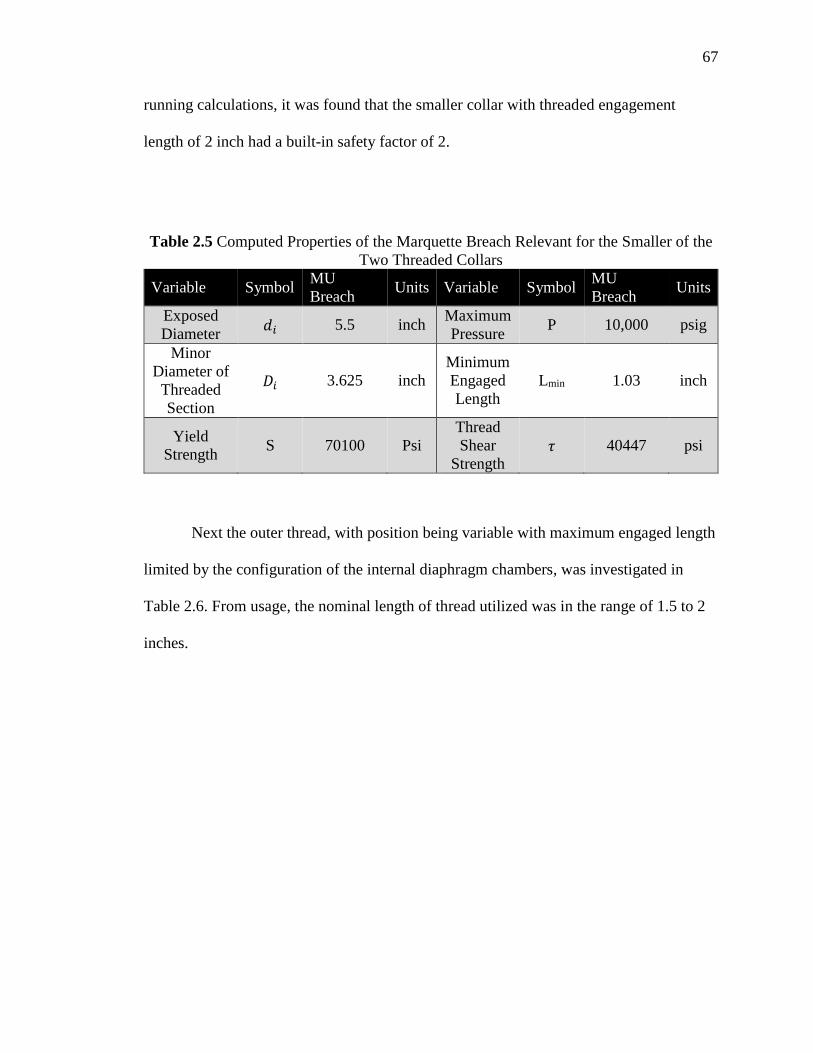
67
running calculations, it was found that the smaller collar with threaded engagement
length of 2 inch had a built-in safety factor of 2.
Table 2.5 Computed Properties of the Marquette Breach Relevant for the Smaller of the
Two Threaded Collars
Variable Symbol MU
Breach Units Variable Symbol
MU
Breach Units
Exposed
Diameter 𝑑𝑖 5.5 inch
Maximum
Pressure P 10,000 psig
Minor
Diameter of
Threaded
Section
𝐷𝑖 3.625 inch
Minimum
Engaged
Length
Lmin 1.03 inch
Yield
Strength S 70100 Psi
Thread
Shear
Strength 𝜏 40447 psi
Next the outer thread, with position being variable with maximum engaged length
limited by the configuration of the internal diaphragm chambers, was investigated in
Table 2.6. From usage, the nominal length of thread utilized was in the range of 1.5 to 2
inches.

68
Table 2.6 Computed Properties of the Marquette Breach Relevant for the Larger of the
Two Threaded Collars
Variable Symbol MU
Breach Units Variable Symbol
MU
Breach Units
Exposed
Diameter 𝑑𝑖 5.5 inch
Maximum
Working
Pressure
P 10,000 psig
Minor
Diameter of
Threaded
Section
𝐷𝑖 7.45 inch
Minimum
Engaged
Length
Lmin 0.5 inch
Yield
Strength S 70100 inch
Force
Applied 𝑭𝒓𝒆𝒒 237583 lbf
Given this information it is suggested that the minimum engaged thread be at least
1.25 inches in length. Reviewing all information, the maximum safety factor for the
breach section was 2 ft. based on adequate thread engagement of the small collar from
Table 2.5. This gave acceptable confidence for safe operation being especially given to
prevent the system from ever reaching pressures beyond the 10ksi working pressure.
To keep the breach sealed, the system was built with several internal sections to
allow for the placement of burst disks. These internal sections mate together through the
aid of O-rings, which are both slightly compliant and air-tight when compressed. To find
the forces applied on each of these O-rings, one can convert the torque applied to the
breach and collar by the torque wrenches into the compressive force felt by the internal
sections and O-rings:
𝐹𝑏𝑟𝑒𝑎𝑐ℎ =𝐹𝑎𝑝𝑝𝑙𝑖𝑒𝑑 𝐿
𝑐𝑓 𝐷𝑜 (2.15)

69
where compressive force between the internal sections and the barrel to the breach,
𝐹𝑏𝑟𝑒𝑎𝑐ℎ, is found via the shortest toque wrench length L, by the force applied 𝐹𝑎𝑝𝑝𝑙𝑖𝑒𝑑, the
outer threaded diameter 𝐷𝑜 and the coefficient of friction 𝑐𝑓 [144]. Back solving for the
force required 𝐹𝑎𝑝𝑝𝑙𝑖𝑒𝑑 to keep the breach sealed without the use of O-rings, the above
equation is manipulated to express 𝐹𝑛𝑒𝑒𝑑𝑒𝑑 in terms of 𝐹𝑟𝑒𝑞:
𝐹𝑛𝑒𝑒𝑑𝑒𝑑 =𝑐𝑓 𝐷𝑜 𝐹𝑟𝑒𝑞
𝐿 (2.16)
Based on these equations, the force required and maximum force achievable was
calculated and expressed in Table 2.7 below.
Table 2.7 Computed Properties for the Applied Torsion Given by the Breach Torque
Wrenches
Variable Symbol MU
Breach Units Variable Symbol
MU
Breach Units
Length of
Moment
Arm 𝐿 18 Inch
Maximum
Application
Force
𝑭𝒂𝒑𝒑𝒍𝒊𝒆𝒅 100 lbf
Coefficient
of Friction 𝒄𝒇 0.2 -
Resultant
Compressive
Force 𝑭𝒃𝒓𝒆𝒂𝒄𝒉 1152 lbf
Threaded
Diameter 𝑫𝒐 7.75 Inch
Engaging
Force
Required
𝑭𝒓𝒆𝒒 237583 lbf
Application
Force
Needed 𝑭𝒏𝒆𝒆𝒅 20624 lbf

70
From these calculations it is clear that the forces applied by the torque wrenches
available are insufficient to the complete sealing of the tank. Therefore, it is of high
importance that compliant O-rings are utilized in order for the breach and chamber to
“self-seal.” For this reason, O-rings before every shot should be clean of particulates and
re-lubricated with vacuum grease.
2.1.2 Barrel
The breach is directly attached to the barrel by means of a threaded collar
assembly. An unslotted 14 ft. barrel, and slotted 12 ft. barrel are interchangeable within
the assembly depending on experimental requirements. Before contacting Physics
Applications Inc. for both the slotted and unspotted barrel, a number of manufacturers
were contacted for the manufacture of both barrels. While a list of other gas gun
manufacturing companies exist, the next closest full service gun company was Thoit
Ingenierie in France [146]; therefore, many parts mentioned in later sections were
purchased from non-specialized manufacturers. While the unslotted barrel was generally
available in the 14 ft. barrel length, manufacturers, including Grand Valley Machining,
which seemed best equipped to handle the construction of our barrel, were was unwilling
to produce a single piece slotted barrel over 12 ft. in length due to boring bar machine
lengths and tolerances. This constraint seemed to be consistent in both the final size made
available through Physics Applications and in other slotted barrels at facilities such as
Sandia’s STAR lab.

71
While the barrel and rollers were purchased from Physics Applications, Inc., the
I-beam, on which the barrel and breach rest, was purchased during the construction of the
Engineering Hall.
Taking a sample from the barrel, it was found that both the breach and barrel were
made from the same material. Utilizing the same pressure vessel equations from before
and now including a much lower weld efficiency to account for the stress concentration
made by the broached (slotted) barrel, one finds that the barrel, given its smaller bore and
walls of equal thickness, is even better equipped to handle the high pressure experienced
during a shot.
Equations (2.1) through (2.8), the equations for shell thickness, are again used to
evaluate the pressures experienced by the barrel under operation. It is known here that the
barrel is made of the same material as the breach. Table 2.8 below summarizes both the
barrel’s known characteristics and resultant operational specifications.
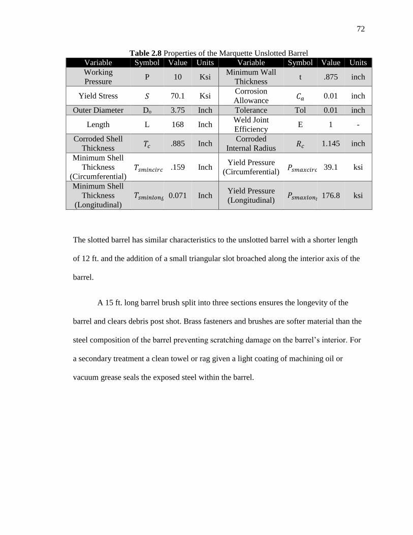
72
Table 2.8 Properties of the Marquette Unslotted Barrel
Variable Symbol Value Units Variable Symbol Value Units
Working
Pressure P 10 Ksi
Minimum Wall
Thickness t .875 inch
Yield Stress 𝑆 70.1 Ksi Corrosion
Allowance 𝐶𝑎 0.01 inch
Outer Diameter Do 3.75 Inch Tolerance Tol 0.01 inch
Length L 168 Inch Weld Joint
Efficiency E 1 -
Corroded Shell
Thickness 𝑇𝑐 .885 Inch
Corroded
Internal Radius 𝑅𝑐 1.145 inch
Minimum Shell
Thickness
(Circumferential) 𝑇𝑠𝑚𝑖𝑛𝑐𝑖𝑟𝑐 .159 Inch
Yield Pressure
(Circumferential) 𝑃𝑠𝑚𝑎𝑥𝑐𝑖𝑟𝑐 39.1 ksi
Minimum Shell
Thickness
(Longitudinal)
𝑇𝑠𝑚𝑖𝑛𝑙𝑜𝑛𝑔 0.071 Inch Yield Pressure
(Longitudinal) 𝑃𝑠𝑚𝑎𝑥𝑙𝑜𝑛𝑔 176.8 ksi
The slotted barrel has similar characteristics to the unslotted barrel with a shorter length
of 12 ft. and the addition of a small triangular slot broached along the interior axis of the
barrel.
A 15 ft. long barrel brush split into three sections ensures the longevity of the
barrel and clears debris post shot. Brass fasteners and brushes are softer material than the
steel composition of the barrel preventing scratching damage on the barrel’s interior. For
a secondary treatment a clean towel or rag given a light coating of machining oil or
vacuum grease seals the exposed steel within the barrel.

73
Figure 2.8 5 ft. sections of the brass barrel cleaning brush.
2.1.3 Sabot
Projectiles launched down the barrel consist of two parts, the sample and the
sabot. In general, there are two types of sabots, one which separates from the projectile
upon leaving the barrel and one which stays attached [147]. The sabot serves as a buffer
between the projectile and gun barrel, preventing damage as well as keeping an airtight
seal behind the projectile [44] [148]. In the case of a separating sabot once the sabot and
projectile have left the barrel, the sabot can be stripped from the projectile by a stripping
box, removed by gas, or fluids forcing the petals of a sabot apart. In cases where there is
a lack of air pushing the sabot apart, imparting a spin on the projectile can often remove
sabot sections with centrifugal force as shown in Figure 2.9.

74
Figure 2.9 A sectioned sabot separating from a long rod penetrator [149].
Marquette’s sabot is a lightweight full-bore plug fitting the interior of the barrel.
Upon releasing gas, the back surface becomes a piston forcing both the sabot and the
flyer it carries down the barrel and into the catch tank. A sabot is destroyed every shot so
the design must be both effective and easy to manufacture. Sabots are made to be
lightweight for optimum acceleration and strong, so as not to deform during travel down
the barrel. The design utilized in experiments thus far is presented below in Figure 2.10
with right to left orientation indicative of sabot travel direction when facing the gun as in
Figure 2.1.
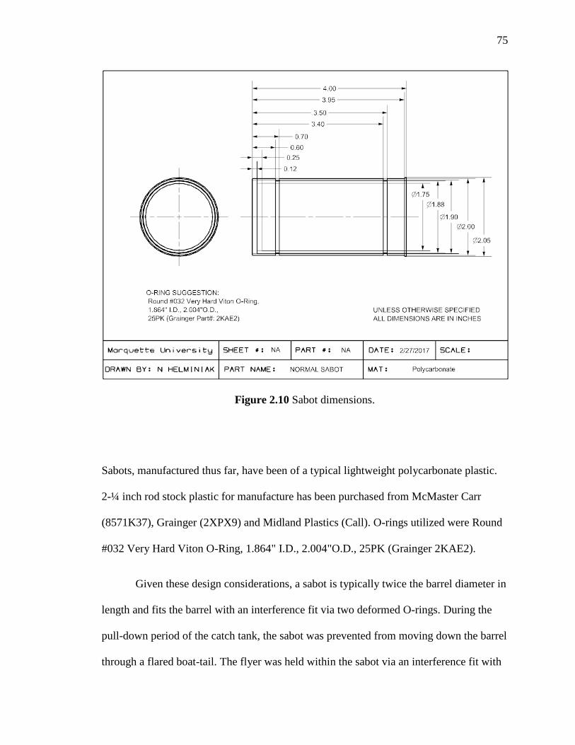
75
Figure 2.10 Sabot dimensions.
Sabots, manufactured thus far, have been of a typical lightweight polycarbonate plastic.
2-¼ inch rod stock plastic for manufacture has been purchased from McMaster Carr
(8571K37), Grainger (2XPX9) and Midland Plastics (Call). O-rings utilized were Round
#032 Very Hard Viton O-Ring, 1.864" I.D., 2.004"O.D., 25PK (Grainger 2KAE2).
Given these design considerations, a sabot is typically twice the barrel diameter in
length and fits the barrel with an interference fit via two deformed O-rings. During the
pull-down period of the catch tank, the sabot was prevented from moving down the barrel
through a flared boat-tail. The flyer was held within the sabot via an interference fit with
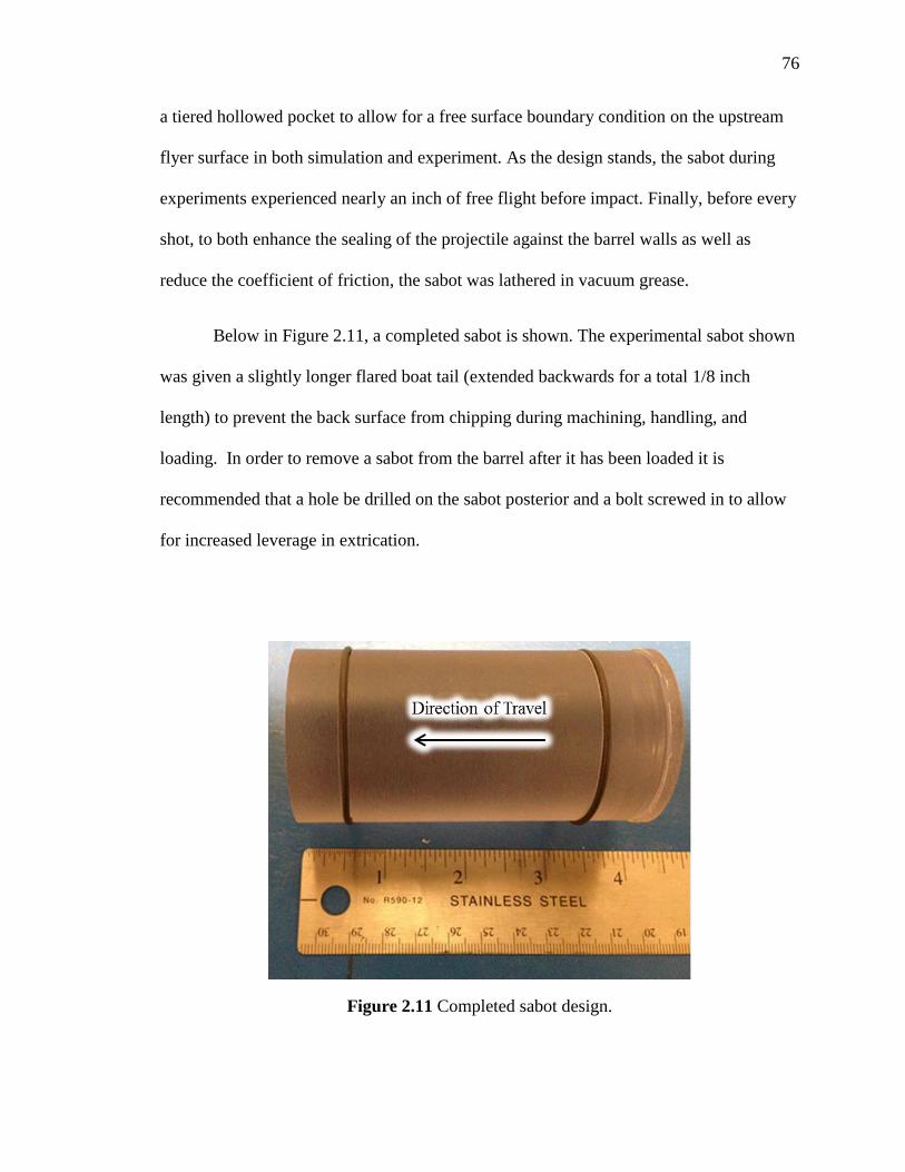
76
a tiered hollowed pocket to allow for a free surface boundary condition on the upstream
flyer surface in both simulation and experiment. As the design stands, the sabot during
experiments experienced nearly an inch of free flight before impact. Finally, before every
shot, to both enhance the sealing of the projectile against the barrel walls as well as
reduce the coefficient of friction, the sabot was lathered in vacuum grease.
Below in Figure 2.11, a completed sabot is shown. The experimental sabot shown
was given a slightly longer flared boat tail (extended backwards for a total 1/8 inch
length) to prevent the back surface from chipping during machining, handling, and
loading. In order to remove a sabot from the barrel after it has been loaded it is
recommended that a hole be drilled on the sabot posterior and a bolt screwed in to allow
for increased leverage in extrication.
Figure 2.11 Completed sabot design.

77
Later sabot designs may wish to incorporate an additional O-ring at the posterior
end in order that two O-rings remain within the barrel during impact for pressure shear.
In designs where velocity is of increasing importance, an internal cavity could also
theoretically be made within the sabot to reduce mass.
2.1.4 Target Tank
The target tank is limited in the peak pressure it can withstand, as the catch tank that
connects directly to the target tank is rated to withstand 125 psig.
The barrel ends within the target tank. A flange, shown in Figure 2.12, attached to
the target tank contains a recessed internal O-ring, which allows the airtight mating of the
barrel to the target tank (vacuum grease has been placed around this fitting to prevent
residual leaking). Each barrel has a unique flange, which must be replaced when
switching out barrels.

78
Figure 2.12 Flange mating the barrel with the target tank.
In order to find the theoretical torque needed with O-rings, one first needs to
know the gun recoil velocity. From “Ballistics: theory and design of guns and
ammunition” [150], one finds that the primary contributors to gun recoil force is the
projectile and gas mass accelerating down and leaving the gun barrel. This force is
calculated in section 4.7 and found for peak experimental parameters to be ~20 kips
(89.13kN).
Using Mechanical Engineering Design [144], one can find the pre-torque load
required by the mating flange. First the bolt stiffness is calculated:

79
kb =Ad At E
Adlt+Atld (2.17)
where kb, is the bolt stiffness, Ad is the nominal bolt diameter, At is the bolt tensile stress
area, E is the modulus of elasticity, lt is the bolt threaded length, and ld is the unthreaded
bolt length. Next the member stiffness is calculated using the method of Conical Frusta,
which breaks up the loading of a bolted material by location and material. Each section
stiffness is calculated using:
kn =0.5774 π E d
ln ((1.155t+D−d)(D+d)
(1.155t+D+d)(D−d)) (2.18)
where 𝑘𝑛 is the member stiffness of a section, E is the modulus of elasticity, d is the bolt
diameter, t is the section thickness, and D is the minor Frusta diameter. The method
chosen often requires the addition of multiple spring rates which are added in this way:
1
km=
1
k1+
1
k2+
1
k3+ ⋯ (2.19)
where the inverse of the total member stiffness is the sum of the inverse of each section
member’s stiffness. From these, one can characterize stiffness with a constant, C:

80
C =kb
kb+km (2.20)
The preload is then calculated:
Fi = 0.75 At Sp (2.21)
where Fi is the bolt preload, At is the tensile area of the bolt, and Sp is the proofing
strength of the bolt. This can be expressed as a torque:
T = K Fi d (2.22)
where T is torque, and K is the bolt surface constant. In addition, the minimum number of
bolts N can be found:
N =C nL Pi
Sp At−Fi (2.23)

81
With a resultant yielding factor of safety np:
np =Sp At
C (Pi
N⁄ )+Fi
(2.24)
The results of these calculations are included below in Table 2.9.
Table 2.9 Pre-load and Torque Calculations for the Barrel Mating Flange
Input
d, Bolt Diameter (in) 0.5 E, Young's Modulus
(Mpsi) 30
lt, Threaded Length (in) 1.35 K, Torque Factor (-) 0.2
ld, Unthreaded Length (in) 0.887 Sp, Proof Strength (kpsi) 85
Ar, Minor Area (in2) 0.126 Pi, Separating Force (kip) 20
At, Tensile Area (in2) 0.142 N, Bolts (-) 8
Frusta Layer Properties
Layer (#) d (in) D (in) t (in) E (Mpsi)
1 0.5 0.75 0.7855 30
2 0.5 1.342 0.15 30
3 0.5 0.892 0.5125 27.5
4 0.5 0.75 0.123 30
Output
km (Mlbf/in) 10.123 N Min (FOS 1) 2.313
kb (Mlbf/in) 2.138 Fi Preload (kips) 9.046
C Stiffness Constant (-) 0.174 T1 Pre-torque (lb*ft) 75.384
np Yielding FOS (-) 1.272 T2 Pre-torque (lb*ft) 80.404

82
The target tank, shown in context within Figure 2.1, contains the apparatus from
which to both set experiments and prepare diagnostics. It is where the actual experiments
take place. Around the circumference of the target tank are six diagnostic ports, two 2-
11½ NPT and four ½-14 NPT ports. Currently, two of the ports are utilized, one as a re-
pressurization valve and the second as a diagnostic port (shown in Figure 2.13).
Figure 2.13 Target tank with external features and teardown of the bulkhead.
The re-pressurization port shown in Figure 2.14, allows for both the target tank
and catch tank to be brought to atmospheric pressure without the need to fire or manually
disassemble components. For optimal performance, the ball within the ball valve should
be occasionally lubricated with a dab of vacuum grease to ensure a tight seal. The brass
muffler decreases noise when the chamber re-pressurizes and provides a much larger
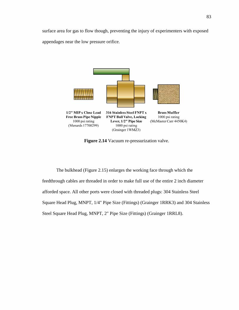
83
surface area for gas to flow though, preventing the injury of experimenters with exposed
appendages near the low pressure orifice.
Figure 2.14 Vacuum re-pressurization valve.
The bulkhead (Figure 2.15) enlarges the working face through which the
feedthrough cables are threaded in order to make full use of the entire 2 inch diameter
afforded space. All other ports were closed with threaded plugs: 304 Stainless Steel
Square Head Plug, MNPT, 1/4" Pipe Size (Fittings) (Grainger 1RRK3) and 304 Stainless
Steel Square Head Plug, MNPT, 2" Pipe Size (Fittings) (Grainger 1RRL8).

84
Figure 2.15 Bulkhead, dimensions, and components.
Within the target tank, there are four main assemblies utilized in every launch: the
target plate, velocity block, target gage plug, and blast shield. After the velocity block is
placed within the target tank, the target plate should be affixed and set in a configuration
parallel to the muzzle. A dial indicator cantilevered off of a plug sitting within the barrel,
as shown in Figure 2.16 accomplishes this task.

85
Figure 2.16 Dial indicator to align the target plate and a mounted sample.
To ensure that the target is seated properly the dial is spun around the diameter of the
target plate for a minimum of twelve sample points (four between each bolt). These
sample offsets are then input into the equation below:
𝑅𝐴𝑙𝑖𝑔𝑛 = tan−11
𝑁 ∑ (𝑥𝑖−𝜇)2𝑁
𝑖=1
𝐿𝑅𝑎𝑑𝑖𝑎𝑙 𝐴𝑟𝑚 (2.25)
where RAlign is the radial alignment, N is the number of samples, xi is the individual
sample, µ is the average value of the samples, and LRadial Arm is the length of the radial
arm from the center of the plug to the center of the dial. A sample table of calculations is
included below in Table 2.10.

86
Table 2.10 Sample Target Plate Alignment Calculation
Position Measurement (inch) Position Measurement (inch)
1 0.049 7 0.050
2 0.050 8 0.051
3 0.050 9 0.050
4 0.050 10 0.050
5 0.050 11 0.051
6 0.050 12 0.051 Measurements are taken ± 0.0005 inches
LRadial Arm (inch) Variance (inch2) Ralignment (mill radians)
3.225 0.001154 0.3580
This yields the radial alignment of the target plate. A sample mounted to this plate
(Figure 2.17) can then with careful affixation be made parallel with the gun barrel. It
should be mentioned here that mounted targets should be affixed with screws with stress
concentrations machined to allow the experiments to break away from the target mount
plate without damage.
Figure 2.17 Sample mounted on the target plate.

87
Once the sample is secured onto the target plate, a blast shield (Figure 2.18) is placed to
rest on the center track. This shield surmounts the target plate and extends down-range
into the catch tank, protecting exposed wires along the walls of the target tank and
directing debris to travel the length of the catch tank.
Figure 2.18 Blast shield CAD model and completed design.
2.1.5 Catch Tank
Affixed to the target tank, by means of eight steel bolts, is the catch tank
manufactured by International Product Specialists Inc. (dimensions included in Appendix
A). This tank is rated to a maximum pressure of 125 psig, well below the expected peak
end pressures of both nitrogen and helium 10,000 psig shots. As before using section 4.7,
one can calculate the pre-torque required on the bolts using equations (2.17) to (2.24).
The results of these equations are tabulated below in Table 2.11.

88
Table 2.11 Pre-load and Torque Calculations for the Target/Catch Tank Interface
Input
d, Bolt Diameter (in) 1 E, Young's Modulus (Mpsi) 30
lt, Threaded Length (in) 4 K, Torque Factor (-) 0.2
ld, Unthreaded Length (in) 2 Sp, Proof Strength (kpsi) 85
Ar, Minor Area (in2) 0.551 Pi, Separating Force (kip) 20
At, Tensile Area (in2) 0.606 N, Bolts (-) 8
Frusta Layer Properties
d (i) D (in) t (in) E (Mpsi)
1 1.5 2.7565 30
1 3.479 0.8575 30
1 3.693 0.185 0.0007
1 1.5 1.714 30
Output
km (Mlbf/in) 0.040 N Min (FOS 1) 3.069
kb (Mlbf/in) 3.280 Fi Preload (kips) 38.633
C Stiffness Constant (-) 0.988 T1 Pre-torque (lb*ft) 643.875
np Yielding FOS (-) 1.253 T2 Pre-torque (lb*ft) 624.450
The target tank has been modified both internally, to contain impacts, and
externally, to hold the vacuum system (Figure 2.19). The target tank sits atop four rollers
which allows access to the target tank or the catch tank man-way (80 foot-pounds pre-
load torque required). The rollers also keep the catch tank aligned to the target tank,
allowing the tanks to be quickly reconnected before a shot.

89
Figure 2.19 The catch tank: attaching the vacuum mount plate.
For future reference if needed, a drawing of the vacuum mount points is included in
Figure 2.20 below, as this information is not available in any reference manuals or
guides.
Figure 2.20 Agilent vacuum pump mounting points.

90
In order to slow the projectile and prevent penetration of the projectile out the rear
of the catch tank, a swinging impact plate has been installed with relevant dimensions
given in Figure 2.21 below.
Figure 2.21 Impact plate.
This system relies on the safe transfer of impact load into the plate, then, through
chains and into bolts mounted to the catch tank. An initial estimate of impact force is

91
difficult because while the initial momentum of the projectile is well characterized, the
duration of impact and the final impact momentum is not. In any case, peak impact
should occur if the projectile is launched using helium (as hydrogen is not advised)
without hitting a target.
For an initial conservative analysis, one may first assume that the impact time was
directly related to the sound speed and length of the polycarbonate sabot. Second, one
assumes that the projectile within this time span loses all momentum. With this in mind,
the following equation is generated:
timpact ≈Lsabot
ao (2.26)
where timpact is the time of impact, Lsabot is length of the sabot, and ao is the sound speed of
the projectile. Let us assume first assume a typical 4 inch (10.16 cm), 0.25 kg
polycarbonate projectile (with a sound speed of 2270 m/s) traveling at the maximum
expected velocity of 1.1km/s impacts the center of a steel plate. Using this information in
conjunction with equation (2.26) one finds an impact time of 47.78 µs and initial
momentum of 275 kg m/s. Observing Newton’s Second Law [145], one can see that force
is related to the change in momentum over a change in time:
F =d(mV )
dt (2.27)
92
where F is the force of impact, m is the mass of the impactor, V is the velocity of the
impactor and t is the time of impact. Since the impact above can be assumed to act in a
single direction, the vector form is reduced to a single scalar equation which yields an
impact force of 61411 kN. Over the 81 cm2 area of the impact, one finds a pressure of
760 MPa, which is over the typical yield of steel (~550 MPa). If this were the case,
impacts might succeed in deforming or penetrating the steel and complete perforation of
the plate would likely transfer negligible force onto the chains. In reality, the plate has
both compliance in its’ rubber layers and an ability to deform and swing with the impact.
These two factors amongst others raise the duration of impact and decrease the force of
impact felt by the catch plate.
To ensure that penetration is not a problem, one can use the Lambert and Zukas
model [152] for ballistic penetration into rolled homogenous armor (hardened steel). One
can ensure that the plates can handle impact using the ballistic limit equation below:
𝑉𝑙 = (𝑙
𝑑)0.15
(400,000)√𝑑3
𝑚[𝑡
𝑑(sec (𝜃))0.75 + exp (−
𝑡
𝑑(sec(𝜃))0.75) − 1] (2.28)
where 𝑉𝑙 is the velocity at which a long rod projectile will penetrate, l is the projectile
length, d is the projectile diameter, m is the mass of the projectile, t is the thickness of the
plate, and θ is the angle of impact [150]. Using this equation and assuming the projectile
is a typical sabot with length of 4 inches (10.16 cm) striking the full thickness of the

93
steel, the estimated ballistic limit is around 700 m/s. This is an overestimate as the
projectile has a yield strength much lower than that of the steel. Even when carrying a
sample of steel, the length of the sample is typically much lower than that of the sabot. In
addition the impact plate in made in a layered configuration as seen in Figure 2.21. By
layering the steel plates kinetic energy imparted by the projectile is greatly reduced.
Should experiments within Marquette ever investigate penetration mechanics of long rod
penetrators with length exceeding ¼ the length of the sabot, additional calculations
should be performed to ensure safety. For typical experiments, including normal impact,
pressure shear and shock consolidation, section 4.5 suggests that a projectile might reach
a peak velocity of 720 m/s for nitrogen (at 10,000 psig or 68,947.6 kPa charge) and 1,120
m/s for helium. To ensure that the impact can withstand these peak velocities, an
additional steel plate of thickness 0.5 inches (1.27 cm) should be affixed to the man-way
as an additional layer of protection. It is also suggested that for velocities greater than
half of the above ballistic limit additional calculations be performed using either ballistic
penetration formulations and/or CTH calculations.
Assuming the projectile does not penetrate into the impact plate, one could
assume that the momentum between the 0.25 kg projectile and 45 kg plate could transfer
perfectly. In order to calculate this, it is assumed that the impact is perfectly elastic,
functioning according to the below equation:
mprojvproj + mtargetvtarget = mtotalvtotal (2.29)

94
The momentum of the system of the system is the same as before, but the velocity of the
system is lowered from the 1.1 km/s velocity of the projectile to a total velocity of
6.1m/s. Time scale of impact also increases as the plate is allowed both to deform and
swing. Assuming the chains linearly decelerate the impact plate over the ~ 5 cm travel
distance of the plate, one finds a longer impact time of 8.33 m/s. Again solving for
impact force, one finds a much lower force of 33 kN acting on the plate. The linear
deceleration of the plate over estimates the time of impact, as chains will likely exert
much greater deceleration forces the further the plate swings back, rather than a constant
deceleration. However given the two time estimates it is likely that the lower limit will
more accurately represent the loading behavior of the set of four chains and eight bolts
given the compliance of the rubber on the plate and its ability to swing.
Figure 2.22 Range of pressure loads experienced by the chains securing the catch tank
impact plate.

95
Hanging the plates require a set of eight 0.5 inch grade 4 bolts, each with a
minimum tensile strength of 115 kpsi (792.9 MPa), that connect the plate to sets of chains
supporting the impact plate within the target tank. Using the below formulas assuming
the lower limit of imparted force [144]:
Shear Stress =F
π r2 (2.30)
τshear strength = 0.577 σmin tensile (2.31)
one finds that use of four bolts yields a safety factor of 2.64. (8MPa vs. 457.5MPa)
Between the bolts and plate are four chains (Menards 3/16 inch proof coil chain)
each able to support 3.6 kN (800 lbf) of static load. While these are appropriate for shots
up to 1500 psig, for greater pressures, these should be switched out for chains each
capable of supporting 13.3 kN (5,000 lbf) for operational safety. Additionally a second
steel plate should be installed on the inside of the man-way door located on the rear of the
target tank as a secondary stopping method.
Of the various analyses, penetration is difficult to characterize, especially for
multicomponent or asymmetric construct. Calculations above are a rough indication of
the target tank’s ability to stop an unimpeded projectile, which should never occur (as the
projectile should first impact a target, losing energy). With this in mind, care should be
taken in experiments near the upper limits of the Marquette 2-inch gas gun especially if
researchers ever choose to use helium to ensure the safety of equipment and personnel.
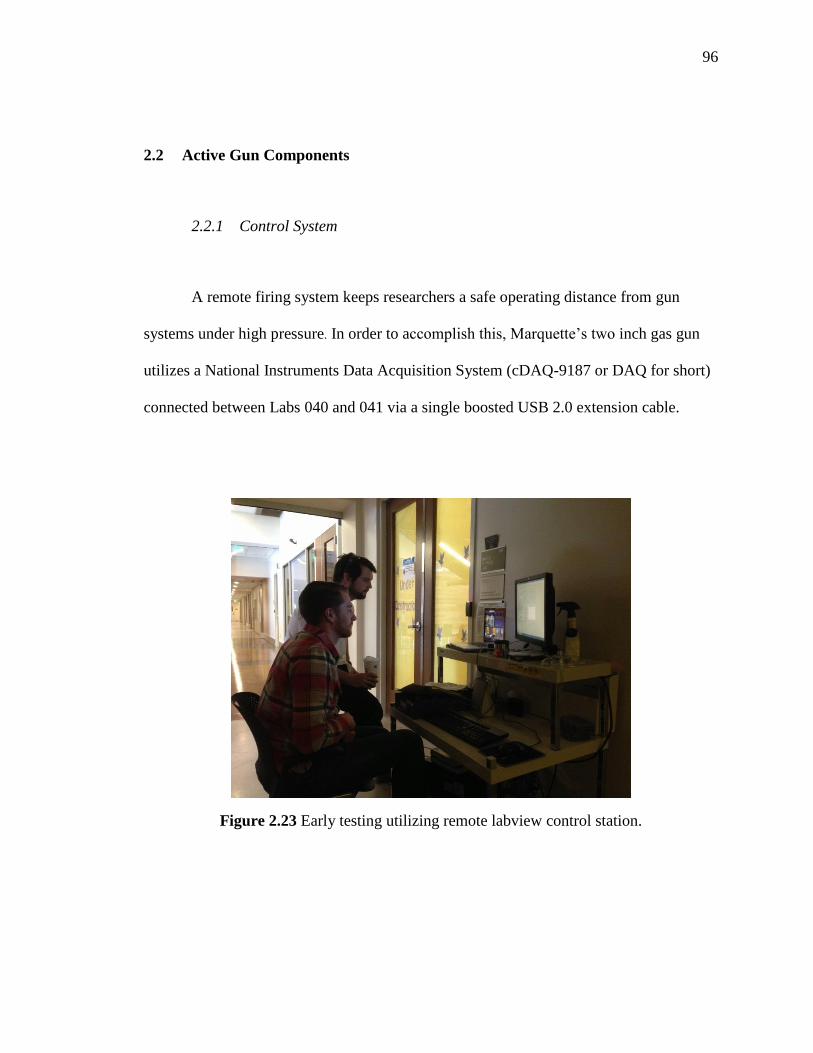
96
2.2 Active Gun Components
2.2.1 Control System
A remote firing system keeps researchers a safe operating distance from gun
systems under high pressure. In order to accomplish this, Marquette’s two inch gas gun
utilizes a National Instruments Data Acquisition System (cDAQ-9187 or DAQ for short)
connected between Labs 040 and 041 via a single boosted USB 2.0 extension cable.
Figure 2.23 Early testing utilizing remote labview control station.

97
The DAQ is housed within an electrical control box (Figure 2.24) mounted directly to the
I-Beam supporting the 2 inch gun. The internals of this system consist of the DAQ itself,
a power distribution board, relays controlling AC Voltage, a DC Power supply, and a
number of USB AC to DC converters for monitoring valve status.
Figure 2.24 Main electrical control box.

98
The DAQ can both send and receive data through up to eight custom function
cards. Currently the DAQ is equipped with four cards listed with name functionality and
purpose in Table 2.12.
Table 2.12 National Instuments Modules
Name Functionality Purpose
NI 9481 4 Channel Single Pole Single Throw
(SPST) Relay With support for:
30 VDC (2 A), 60 VDC (1 A), or 250 VAC
(2 A)
The first relay module is
used in switching the
primary Swagelok electric
valves utilized for change
system pressure
distribution.
NI 9482 4 Channel Electromagnetic Relay
(An updated NI 9481) With support for:
60 VDC (1 A), or 250 VAC (1.5 A)
A second relay module
controls valves for: running
the Haskel, sealing the catch
tank from the vacuum
system, and controlling the
vacuum pump
NI 9205 32 Channel (16 Diff) ±10 VDC Voltage
Module
With support for:
250 ksamples/sec and 16 bit resolution.
The first voltage module
monitors valve (Open,
Closed, Running) status 0 or
5V from the Swagelok
valve.
NI 9205 32 Channel (16 Diff) ±10 VDC Voltage
Module
With support for:
250 ksamples/sec and 16 bit resolution.
The second voltage module
takes measurements from 0-
5 volts down to the millivolt
range.
These switches and voltage monitors are displayed on the receiving computer through
LabVIEW software. From here, each of the minor electrical circuits will be discussed
with an electrical circuit diagram.
The first of the circuits is the electrical valve distribution system. The distribution
circuit (shown in Figure 2.25) is one of four circuits which takes AC voltage from the

99
wall outlet and uses it to power both a 12 VDC power supply and the electrical valves
themselves. This circuit is contained mainly within the electrical control box but does
extend into the electrical high pressure valves by PVC conduit. In order to control the
valves, signals from each terminal will relay power from the 12 VDC power supply.
When excited, the relay will either drive the electrical valve open or closed. While
powered, the valves will send out a 120V electrical signal from one of three lines,
“Open”, “Closed” or “Running” to indicate the status of the valve. In order to read this
signal, a number of USB power converters were utilized to transform the 120 VAC to 5V
DC. The resultant signal from the USB power converters do not send out a straight 0-5
VDC signal, but instead convert the input AC current to a DC square wave with a peak 5
VDC amplitude.
Figure 2.25 Single 10ksi distribution electrical system utilizing NI 9481 and 9205
modules.

100
In order to control the vacuum remotely (see Figure 2.26 circuit), a 12 VDC
signal (open or closed by the National Instruments DAQ) is sent from the electrical
control box to a breakout box containing a high amp electromagnetic relay. This relay
makes or breaks a high amperage 120 VAC current circuit (designated by a labeled
power outlet within the lab) controlling whether the Agilent Vacuum pump is on or off.
Figure 2.26 Vacuum pump switch.
Much like the vacuum pump, the Haskel is controlled via a breakout box, shown
in Figure 2.27 below, which sends a 12 VDC signal to a relay which switches 120 VAC
power on and off to the solenoid controlling the air pressure driving the Haskel pressure
booster.

101
Figure 2.27 Haskel power circuit operating the MAC solenoid.
Signals coming from the two high pressure transducers and KJL vacuum
transducer are sent directly into a second NI 9205 Module. Since the KJL vacuum
transducer is powered by an external power supply, a pair of resistors connecting the
signal to the ground of the NI module were added in accordance with recommendations
given in Figure 2.28 below.

102
Figure 2.28 National Instruments signal connection guide [153].
From the LabView terminal, control of the gun is managed through two main
graphical interfaces. The first is a diagnostics screen (Figure 2.29), which provides
oscilloscope readings, errors from various modules and some legacy controls from the
older flow control system to the Haskel.

103
Figure 2.29 Operator debug screen.
The second gun control is a panel with a graphical representation of the system
(Figure 2.30). It is intended that this screen be easier to understand than the previous
diagnostics screen with interactive valves and indicator lights, which map the flow of gas
into and out of the chambers, as well as graphical chambers which fill as a percentage of
set pressures. It is important that users use only the Debug or Pictographic display while
operating the gas gun (this includes pretests and experiments)!

104
Figure 2.30 Pictographic gun control display.
Behind the running graphical user interfaces (GUIs) are a number of logical systems for
each of the DAQ Modules. These systems use LabVIEW software to both send and
receive data from the NIDAQ housed in the electrical control box.
The pressure distribution controls shown in Figure 2.31 utilize two DAQ
Channels to both send and receive data from the four electrical high pressure valves.
DAQ Module 3 controls the signals sent out to the valves. Within this logical path, the
state of a valve controls a 5 VDC solenoid sending 120 VAC power to either close or
open a valve. When a valve enters a state of “Open” (Channels 0-4), “Running”
(Channels 8-12), or “Closed” (Channels 4-8), an electrical 120 VDC signal is sent back to
the DAQ through a 120 VAC to 5 VDC USB transformer. These signals are used as limit
thresholds to return the valve state to the user in the form of running lights.

105
Figure 2.31 Pressure distribution control system.

106
The control loop in Figure 2.32 controls the remainder of the switch state
components on the Marquette gas gun. As can be observed, the three channels in use
include the Aglient vacuum pump (Channel 1), the vacuum safety valve separating the
vacuum pressure transducer and Aglient pump from high pressures during shots (Channel
2), and finally the control switch for the Haskel pressure booster (Channel 3). As with the
pressure distribution controls, the status of these values are also returned to the user
display with running lights.
Figure 2.32 Haskel, safety vacuum valve, and Agilent pump switch control.
Signal data from each of the pressure transducers arrives to the DAQ in the form
of voltages ranging from 0-5 VDC. These signals are converted to pressure units through
the use of linear transformation equations (Figure 2.33). High side breach pressure
(Channel 0), low side breach pressure (Channel 1), and vacuum pressure (Channel 2) are
each fed into a data collection table, which collects data each second from the time the

107
control system is initialized until the system is stopped. Before stopping the Labview run,
it is important to save data for later analysis. Data is output in the form of three space
delimited files including time of collection and computed pressure.
Figure 2.33 Signal data collection from the high and low pressure chambers as well as
vacuum pressure.
Finally a legacy Haskel flow controller is included (Figure 2.34). While this
system is not presently utilized, it proves that our system has the ability to send and
receive additional serial signals through the USB extension from a RMA-LP2600A
Omega flow controller. This was not a straightforward procedure and required decreasing
the loop cycle time, a VISA Serial connection and multiple command selector loop. It is
intended that by inclusion of this legacy system if additional serial signals are required in
the future, researchers will have a guide upon which to look back.

108
Figure 2.34 Legacy Haskel flow control diagram.
The “Prolific” serial to USB connector no longer was supported by Windows 10,
but a reversion of device driver to version 3.3.2.102 within the device manager made the
device operable.
2.2.2 Pressurization System
The pressurization system takes gas provided through either the building’s
pressurized air supply or a nitrogen gas tank and increases the pressure through a
“Haskel” gas booster system. The system, as suggested, only requires air pressure to

109
operate, using differences in piston area (a 62/152 area ratio) and a network of check
valves to pressurize during both the forward and return stroke of the “dual stage” Haskel.
This pressurization system was convenient, as it was driven solely through gas pressure
without a need for electronics; a conceptualization of the internal views is shown below
in Figure 2.35.
Figure 2.35 Conceptualized artistic rendition of the pressure booster’s interior
mechanism.

110
In order to control the pressurization system, three main requirements needed to
be addressed. First, the Haskel required a driving gas. As Marquette had a built-in air
system, a line was installed directly to the Haskel’s air inlet. Marquette’s air supply has
been known in the past to contain water condensed out of the compressed air, especially
after muggy summer months. Marquette’s Shock Physics lab, situated in the basement of
Engineering Hall, is one of a few locations in which the water will collect. To mitigate
rust damage to the Haskel, both a release valve and water separator were added.
Secondly, to turn the Haskel on and off, a MAC solenoid valve was placed within the
Haskel’s air power supply line. The solenoid only allows air flow when electrically
charged and fails in a “fail close” configuration. This means that in the event of an
outage, or the requirement for an experiment to immediately end, interrupted power
prevents the experiment from proceeding out of the researcher’s control. Finally, gas can
be supplied to the Haskel by an alternative method to charging from shop air taken from
the same supply as the gas powering the Haskel. This secondary means uses pressurized
nitrogen or helium from a high-pressure tank, which allows for faster charging as well as
improved shot performance. The aforementioned design is shown below in Figure 2.36.

111
Figure 2.36 Pressurization system reference sheet.
In addition to the power and supply air to the Haskel, the system also includes a
line which extends back to the vacuum system. This extra gas line feeds the vacuum
safety valve (discussed later in section 2.2.7). Low-pressure connections consisting of
NPT wound in 2-3 turns of white PTFE pipe tape for a better air seal. While the NPT
galvanized fittings were inexpensive and relatively easy to assemble, their pressure rating
was too low to use for high-pressure applications. So in cases where necessary Swagelok
components were utilized. After components were assembled, connections were checked
for leaks using “Mega Bubble Leak Detector,” a blue solution which bubbled around
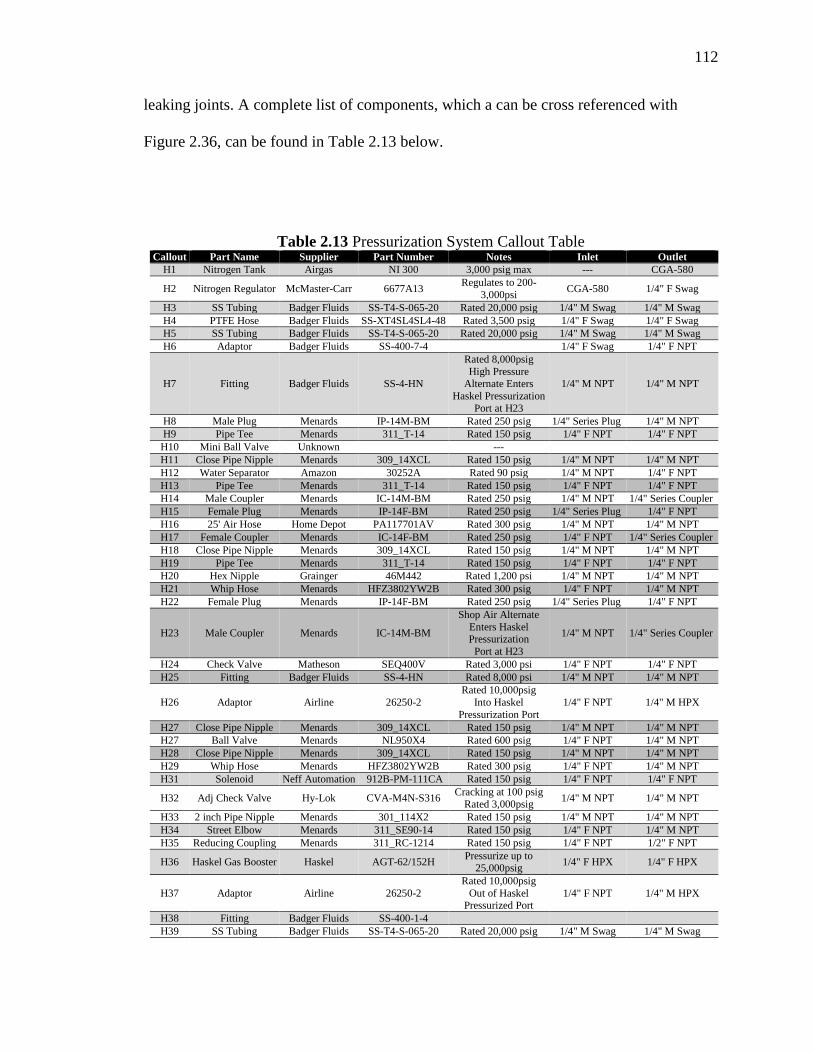
112
leaking joints. A complete list of components, which a can be cross referenced with
Figure 2.36, can be found in Table 2.13 below.
Table 2.13 Pressurization System Callout Table Callout Part Name Supplier Part Number Notes Inlet Outlet
H1 Nitrogen Tank Airgas NI 300 3,000 psig max --- CGA-580
H2 Nitrogen Regulator McMaster-Carr 6677A13 Regulates to 200-
3,000psi CGA-580 1/4" F Swag
H3 SS Tubing Badger Fluids SS-T4-S-065-20 Rated 20,000 psig 1/4" M Swag 1/4" M Swag
H4 PTFE Hose Badger Fluids SS-XT4SL4SL4-48 Rated 3,500 psig 1/4" F Swag 1/4" F Swag
H5 SS Tubing Badger Fluids SS-T4-S-065-20 Rated 20,000 psig 1/4" M Swag 1/4" M Swag
H6 Adaptor Badger Fluids SS-400-7-4 1/4" F Swag 1/4" F NPT
H7 Fitting Badger Fluids SS-4-HN
Rated 8,000psig
High Pressure Alternate Enters
Haskel Pressurization
Port at H23
1/4" M NPT 1/4" M NPT
H8 Male Plug Menards IP-14M-BM Rated 250 psig 1/4" Series Plug 1/4" M NPT
H9 Pipe Tee Menards 311_T-14 Rated 150 psig 1/4" F NPT 1/4" F NPT
H10 Mini Ball Valve Unknown ---
H11 Close Pipe Nipple Menards 309_14XCL Rated 150 psig 1/4" M NPT 1/4" M NPT
H12 Water Separator Amazon 30252A Rated 90 psig 1/4" M NPT 1/4" F NPT
H13 Pipe Tee Menards 311_T-14 Rated 150 psig 1/4" F NPT 1/4" F NPT
H14 Male Coupler Menards IC-14M-BM Rated 250 psig 1/4" M NPT 1/4" Series Coupler
H15 Female Plug Menards IP-14F-BM Rated 250 psig 1/4" Series Plug 1/4" F NPT
H16 25' Air Hose Home Depot PA117701AV Rated 300 psig 1/4" M NPT 1/4" M NPT
H17 Female Coupler Menards IC-14F-BM Rated 250 psig 1/4" F NPT 1/4" Series Coupler
H18 Close Pipe Nipple Menards 309_14XCL Rated 150 psig 1/4" M NPT 1/4" M NPT
H19 Pipe Tee Menards 311_T-14 Rated 150 psig 1/4" F NPT 1/4" F NPT
H20 Hex Nipple Grainger 46M442 Rated 1,200 psi 1/4" M NPT 1/4" M NPT
H21 Whip Hose Menards HFZ3802YW2B Rated 300 psig 1/4" F NPT 1/4" M NPT
H22 Female Plug Menards IP-14F-BM Rated 250 psig 1/4" Series Plug 1/4" F NPT
H23 Male Coupler Menards IC-14M-BM
Shop Air Alternate
Enters Haskel Pressurization
Port at H23
1/4" M NPT 1/4" Series Coupler
H24 Check Valve Matheson SEQ400V Rated 3,000 psi 1/4" F NPT 1/4" F NPT
H25 Fitting Badger Fluids SS-4-HN Rated 8,000 psi 1/4" M NPT 1/4" M NPT
H26 Adaptor Airline 26250-2
Rated 10,000psig
Into Haskel
Pressurization Port
1/4" F NPT 1/4" M HPX
H27 Close Pipe Nipple Menards 309_14XCL Rated 150 psig 1/4" M NPT 1/4" M NPT
H27 Ball Valve Menards NL950X4 Rated 600 psig 1/4" F NPT 1/4" M NPT
H28 Close Pipe Nipple Menards 309_14XCL Rated 150 psig 1/4" M NPT 1/4" M NPT
H29 Whip Hose Menards HFZ3802YW2B Rated 300 psig 1/4" F NPT 1/4" M NPT
H31 Solenoid Neff Automation 912B-PM-111CA Rated 150 psig 1/4" F NPT 1/4" F NPT
H32 Adj Check Valve Hy-Lok CVA-M4N-S316 Cracking at 100 psig
Rated 3,000psig 1/4" M NPT 1/4" M NPT
H33 2 inch Pipe Nipple Menards 301_114X2 Rated 150 psig 1/4" M NPT 1/4" M NPT
H34 Street Elbow Menards 311_SE90-14 Rated 150 psig 1/4" F NPT 1/4" M NPT
H35 Reducing Coupling Menards 311_RC-1214 Rated 150 psig 1/4" F NPT 1/2" F NPT
H36 Haskel Gas Booster Haskel AGT-62/152H Pressurize up to
25,000psig 1/4" F HPX 1/4" F HPX
H37 Adaptor Airline 26250-2
Rated 10,000psig
Out of Haskel Pressurized Port
1/4" F NPT 1/4" M HPX
H38 Fitting Badger Fluids SS-400-1-4
H39 SS Tubing Badger Fluids SS-T4-S-065-20 Rated 20,000 psig 1/4" M Swag 1/4" M Swag

113
The final system, sans nitrogen/helium pressure tank, can be seen in the below
Figure 2.37.
Figure 2.37 Completed pressurization system.
2.2.3 Distribution System
The distribution system received gases from pressurization, through a series of
valves and regulators, and allows gases both into and out of the breach’s dual diaphragm
system. Immediately upon entering this system, gases are split into three lines: the high
side breach, the low side breach and the pressure relief valve. This pressure relief valve is

114
placed so that system air can never exceed the design working pressure of components
and breach (~10,000 psig). Both high side and low side systems are very similar, each
containing a regulator surrounded both in front and behind by a pair of pressure gauges.
Both of these gauges have been set to allow the gun to be set manually if necessary to
limit the pressure supplied to high and low side. The high side contains a regulator, which
can be set up to 10,000 psig, while the low side is limited to a maximum regulated
pressure of 6,000 psig. Past the sets of gauges, motorized valves with manual override
allow for air to enter into both the high and low side breach cavities. A needle valve
serves to limit the flow, if necessary. Both sides then have pressure transducers, which
monitor the pressures within the chambers, as well as flexible hoses allowing for the
limited motion of both chamber components during disuse, loading, and firing. Each of
these flexible hoses is in fact a pin-pricked hydraulic line hose with the tiny holes placed
along its length to prevent pressure bubbles from forming and rupturing the outer hose
lining. A second set of valves allows for the bleeding of both chamber needle valves;
again, this allows for the reduction of air flow out of the chambers and can be tuned to
the experimenter’s needs. Electronic wiring is contained within PVC tubing and routed
directly to the main gun control box.

115
Figure 2.38 Distribution system reference sheet.
The distribution system, unlike the pressurization system, functioned exclusively
at high pressure. This meant that nearly all components sourced were from Swagelok, a
company specializing in high pressure tubing and fittings. Exceptions to this rule were
the high pressure hosing and omega pressure transducers both rated for the system’s
working pressure. Their fittings utilize a set of two interlocking ferrules with pressure fit
to the piping. These nuts and ferrules made it easy to create custom length piping sections
from component to component. After tightening each of the nuts, a go-no-go gauge,
included on the Swagelok wrench, verified that the nut had been tightened to the correct
torque.
To check the system for leaks, a blue solution of “Mega Bubble Leak Detector”
was utilized. The system was first pressurized to ~100 psig and the solution dabbed onto

116
the connecting sections. In the few areas where pressure leaked out of the system,
bubbles quickly formed and the connections were either tightened (Swagelok) or
removed and retaped (NPT). The complete listing of components within the distribution
system are shown in Figure 2.38 are listed on Table 2.14.
Table 2.14 Distribution System Callout Table Callout Part Name Supplier Part Number Notes Inlet Outlet
D1 SS Tubing Badger Fluids SS-T4-S-065-20 Rated 20,000
psig 1/4" M Swag 1/4" M Swag
D2 FS Tee Badger Fluids SS-400-3 1/4" F Swag 1/4" F Swag
D3 FS to FNPT
Fitting Badger Fluids SS-400-7-4 1/4" F Swag 1/4" F NPT
D4 10k Gauge Badger Fluids PG1-100B-
PG10k-LAOX 1/4" M NPT
D5 FS to MNPT
Fitting Badger Fluids SS-400-1-4 1/4" F Swag 1/4" M NPT
D6 10k Regulator Badger Fluids RS(H)2-02-6-
WP
Rated 10,000
psig
Regulates from 0-10150psig
1/4" FNPT 1/4" FNPT
D7 Automated Ball
Valve Badger Fluids
SS-H83PS4-
42AC
Rated 10,000
psig 1/4" F Swag 1/4" F Swag
D8 Needle Valve Badger Fluids SS-3HNRS4 Rated 10,000
psig 1/4" F Swag 1/4" F Swag
D9 Mounting
Bracket Badger Fluids 304-S1-PP-4T --- ---
D10 High Pressure
Transducer Omega
PX309-10KG5V
Rated 10,000 psig
1/4" M NPT
D11 High Pressure
Hose Badger Fluids 2380N-04V91
Rated 10,000
psig 1/4" M NPT 1/4" M NPT
D12 6k Regulator Badger Fluids KHP1WXB4C2
S200J0
Rated 6,000
psig Regulates from
50-6000psig
1/4" FNPT 1/4" FNPT
D13 6000 Gauge Badger Fluids PG1-100B-
PG6000-LAOX 1/4" M NPT
D14 FS Angle Badger Fluids SS-400-9 1/4" F Swag 1/4" F Swag
D15 10k Pressure
Relief Badger Fluids RV4NF4NF10
Rated 10,000 psig
1/4" F Swag
The finished distribution system, show in Figure 2.39, is shown bolted to the side
of Marquette’s 2 inch gun.

117
Figure 2.39 10ksi pressure distribution system for high and low side breach chambers.
2.2.4 Dual Diaphragm Launch System
In order to conduct experimental research, a gas gun must be able to store a gas
propellant charge up to the desired pressure and, when required, quickly release all
available gas into the barrel. In common practice, an initial thought might be to use a
valve. However, if the valve is opened too slowly, peak pressures kept within the breach
will not affect the sabot as the sabot will begin accelerate away from the breach even if
that pressure is much lower than the breach pressure.
In order to provide the control of a valve with the fast acting requirement of a gas
gun, four major designs, three of which are presented below in , are found in use by other
institutions: fast acting valves; wrap-around breaches; single diaphragm; and double
diaphragm. Fast acting valves [97] as named are quick acting valves, which can be

118
actuated with electricity, gas or explosives. Traditional “fast actuating” valves are low
cost and straightforward to operate; they are also generally the slowest of the four
designs.
Fast Acting Valve Wrap-Around Breach Dual Diaphragm
Figure 2.40 Three common types of firing mechanism. High pressure gas within the
breach can be seen in blue while evacuated volume is colored purple.
Wrap-around breaches use the sabot as the method for blocking gas pressure. A
sabot is typically held in place by a vacuum on the rear surface while a high pressure gas
pressurizes filling an area on the surface of the sabot. This high pressure gas is not
allowed to pass to the front or rear of the sabot by means of two O-rings. To fire the
vacuum on the rear of the sabot is removed and a low pressure gas moves the sabot
forward until the high pressure gas inlet passes the rear O-ring and the gun fires. This
limits design choices, as the material properties and geometry of the sabot must withstand
and seal the full firing pressure from fore and aft section of the sabot, while still being
able to carry the projectile down the barrel. The wrap-around breach is generally more
expensive than a fast acting valve and requires more control to operate correctly.
Diaphragms or burst disks are (often) made of round sheets of material such as
plastic or metal. These disks fail when the pressure differentials, existing across the two

119
surfaces, exceed the strength of the material [98] [151]. Often these disks are
manufactured with stress concentrations on their surfaces allowing them to petal upon
failure, preventing disk material from traveling down the barrel. While single disk
systems are effective, they fail at set pressures once a nominal pressure has been reached,
which leaves less control in the hands of researchers. In order to regain this control loss, a
dual diaphragm system, similar to the one used in this system, affords control at relatively
low cost and high reliability.
Several variations on the burst disk design exist with researchers seeking
increased control over burst disk failure. Burst disk strength can be reduced by heat,
which can be applied through the barrel or directly onto the disks themselves, until failure
without affecting the barrel or breach. Alternately, disks can be punctured with a firing
pin with a variety of punch shapes to initiate failure [94].
In short the dual diaphragm launch system combines the fast acting nature of a
single burst disk with the control of a fast acting valve and is less complex in geometry
than a wrap-around breach. In order to manage the flow of pressurized air in and out of
the dual chambers, a series of four valves and two regulators are utilized. Shots are
conducted through use of a dual diaphragm system with burst disks that fail for a given
pressure differential. Once the system fires, it propels a sabot down the barrel holding a
flyer whose impact is often the beginning of the shock experiment. The sequence of
events used to both prepare and fire a dual diaphragm system is included below in Figure
2.41.

120
Figure 2.41 Dual diaphragm system firing sequence.
2.2.5 Light Gate Assembly
The Light Gate Assembly shown in Figure 2.42, housed within the target tank,
measures flyer velocity upon exiting the barrel. A series of four laser diodes and
collimators, each spaced a nominal distance of 0.75 inches apart, throw by the laser
diodes and are received into light collimators before the signal is boosted giving a set
voltage. Once connected to an oscilloscope, a trigger can be set to record the fall and
subsequent rise in voltage as the flyer and sabot pass through the laser beams. The
velocity blocks are operated by means of a switch placed on the front of the target tank. A
second outlet remains always on to provide power for the oscilloscope.

121
Figure 2.42 Laser gate experimental setup.
The velocity gates are made of machined aluminum blocks with dimensions
shown in Figure 2.43 below. This setup fits laser diodes (ThorLabs F220SMA-B w=633
nm f=10.99mm NA=0.25 SMA Fiber Collimation) which shine visible red light (600
Nm) into laser collimators, which focus light onto detectors (ThorLabs PDA36A Si
Amplified Detector 350-1100mm) on the opposing light gate. Each of the velocity gates
is also fitted with acrylic windows, which helps to protect the collimators and detectors
during a shot.

122
Figure 2.43 Light gate dimensions.
In order to find the projectile velocity, the point is chosen at which the light first
falls below 90% of steady state, to detect the tip of the flyer.
The first four falls should then correspond to the temporal location of the flyer tip.
Knowing the length of the sabot and the distances between laser beams, combined with
the temporal data afforded by the oscilloscope, one can determine the average velocity
(assuming minimal acceleration) experienced by the flyer just prior to collision with the
target.

123
𝑉𝑝𝑟𝑜𝑗𝑒𝑐𝑡𝑖𝑙𝑒 =1
3(∆𝑥𝐺𝑎𝑝𝐴
∆𝑡𝐴+
∆𝑥𝐺𝑎𝑝𝐵
∆𝑡𝐵+
∆𝑥𝐺𝑎𝑝𝐶
∆𝑡𝐶) (2.32)
Figure 2.44 presents data taken from a shot that had a polycarbonate sabot and
conical shaped flyer (390 psig, 0.1187 m, 0.4322 kg). Using the method describe above,
the average projectile velocity was calculated to be 194.4 m/s. Only the first four drops
are used to measure arrival time, as the sabot impacts the material prior passing out of the
first laser’s line of sight. This matches well with an expected velocity of 190.19 m/s and
measured down barrel, Photon Doppler Velocimetry measurement of 197.25 m/s.
Figure 2.44 Light gate reading from a 390 psig, 0.4322 kg shot.

124
Using the time between the projectile’s arrival and exit, one can use the average
velocity to calculate the length of the projectile. Calculations here find a sabot length
between 0.123 m and 0.145 m; these lengths are longer than the length expected by
measurements of projectile length prior to launch. This is likely due to the fact that
compressed gases behind the sabot bend and distort light behind the sabot, making light
gate measurements once the sabot exits the barrel unreliable. With this in mind, light gate
measurements for projectile velocity should only use the arrival signals to determine
projectile velocity.
2.2.6 Photon Doppler Velocimetry and Dynasen Pin System
The Photon Doppler Velocimetry (PDV) and Dynasen pin system shown in
Figure 2.45 are the primary means of collecting experimental data during shock
experiments. These systems can measure velocities and location of projectiles and target
at single instants in time, which are states utilized in conjunction with hydrocode
simulations to determine pressure, stress and temperature states of materials within the
experiment [154].

125
Figure 2.45 Photon Doppler Velocimetry and Dynasen pin system.
The Photon Doppler Velocimetry System (PDV) utilizes lasers emitted at a set
wavelength to track velocities of exposed material surfaces [155] [156]. Light travels at a
constant velocity; this creates interesting phenomena when observers from reference
frames observe a light source traveling both toward and away from the observer. Since as
previously mentioned light remains constant in speed, a wavelength of light, emanating
from a moving source and that same source at rest within the observers reference frame,
will have a different wavelength. In physics, this phenomena is known as the Doppler
Effect, named after Christian Doppler, after he noted the red and blue shift seen in
astrophysical observations of stars [157]. Stars known to emit a certain wavelength of
light will be observed to have wavelength of light shifted depending on whether the star

126
is moving towards or away from the earth (see Figure 2.46). A common way of
experiencing the Doppler Effect is a traveling ambulance siren. Sound waves emanating
through the siren change based on how fast and in what direction the ambulance is
moving.
Figure 2.46 Red and blue shift in stars [158].
This relation between light wavelength and velocity is given by the following equation:
𝑧 =𝜆𝑜𝑏𝑠𝑣−𝜆𝑒𝑚𝑖𝑡
𝜆𝑒𝑚𝑖𝑡 (2.33)
where z is the dimensionless shift (z<0 approaching or blue shift, and z>0 moving away
or red shift), 𝜆𝑒𝑚𝑖𝑡 is the normal wavelength of the object without velocity and 𝜆𝑜𝑏𝑠𝑣 is
the observed wavelength of the object.

127
In the experiments, light is emitted by a collimator onto a target at a set
wavelength. That light travels through the air and hits a sample point. When that point is
in motion, the light reflected back will be shifted based on the velocity of the sample. The
difference between the two wavelengths allows researchers to determine sample velocity.
Light returning from each of the samples depends on two main factors, the angle
at which the light returns from the sample and the surface reflectively. While some
samples such as those made of gold have excellent reflectivity. Polycarbonate and
poly(methyl methacrylate) have near zero reflectivity allowing the majority of light to
pass straight through the sample. This can be solved with a sputter coating machine
(shown below in Figure 2.47).
Figure 2.47 Sputter coating machines in Marquette’s Mechanical Engineering
Department (Technics Hummer 1) and Dental School (MTI GSL-1100x-SPC-12)
respectively.

128
These sputter coaters can deposit a layer of metal such as gold or platinum, though gold
works best for the wavelengths of our lasers. Figure 2.48 displays a typical curve of
sputtering rates for various metals; samples generally were coated for 5-15 minutes for
adequate coverage, though breaks were taken every 2 minutes to ensure samples,
especially those made of plastic would not boil.
Figure 2.48 Sputtering rates for the Marquette Dental School sputter machine [159].
A smooth coated sample, like the acrylic shown in Figure 2.49, is not enough to
guarantee a signal as light must also be returned from the surface to the Fiber optic
collimators.

129
Figure 2.49 Sputter coated acrylic sample.
To ensure a light signal return, a retro reflective surface made by micro machining or
laser etching is recommended. There are two different types of machine-able retro-
reflectors, square and triangular. Other materials such as the retro-reflective beads on
roads were also tested with excellent experimental results. The method of affixing the
beads to the sample surface, however, interfered with readings of actual material
behavior.

130
Figure 2.50 Recommened surface profiles.
Retro-reflective surfaces like those shown in Figure 2.50 allow for return signals even if
the alignment of the emitting collimator is less than perfect.
While PDV in shock physics is used primarily for the measuring of material
surface velocities, a sample investigation is analyzed here for a down barrel velocity
reading taken during a 390 psig, 0.4322 kg shot. As shown below in Figure 2.51
collimators are typically placed on an adjustable bridge, which can orient the collimator
to a target (a traditional target is not included in the setup below). Once oriented, a fast
acting super glue should be used to keep the collimator in place followed by a
manufacturer recommended epoxy to retain orientation during tank pull-down and during
the impact, as superglue shatters at high pressures.
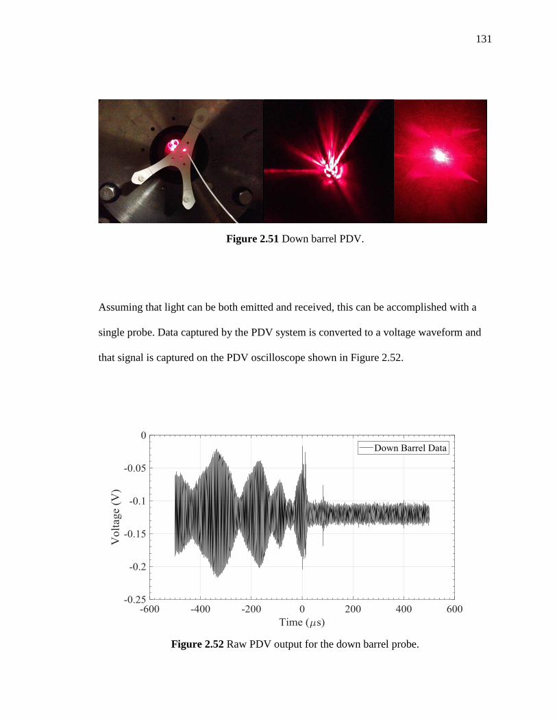
131
Figure 2.51 Down barrel PDV.
Assuming that light can be both emitted and received, this can be accomplished with a
single probe. Data captured by the PDV system is converted to a voltage waveform and
that signal is captured on the PDV oscilloscope shown in Figure 2.52.
Figure 2.52 Raw PDV output for the down barrel probe.

132
Data taken from the PDV may at first seem difficult to interpret; this is due to the
fact that the relevant reading lies within the frequency of the waveforms rather than the
voltage of the signal. To convert the data into more understandable graphs, a Fourier Fast
transform is utilized. This algorithm samples spans of time in data and sorts the
frequencies within that waveform. The output is shown below in Figure 2.53 for the first
1 microsecond of data (in most cases, one should sample in small time spans).
Figure 2.53 Plots of identical datasets displaying FFT output.
From each of these sampled data sets, there will be frequencies which are found
more often than others. Typically the peak data is the correct signal, but in some cases it
might be the second or even third highest peak. Since one must calculate the FFT to find
peak data and this calculation is time consuming, FFTs completed by this researcher save
a sorted ranking of each FFT per time step. Once the FFT has run its course, the
following equation is utilized, shown here for the highest per time sample:
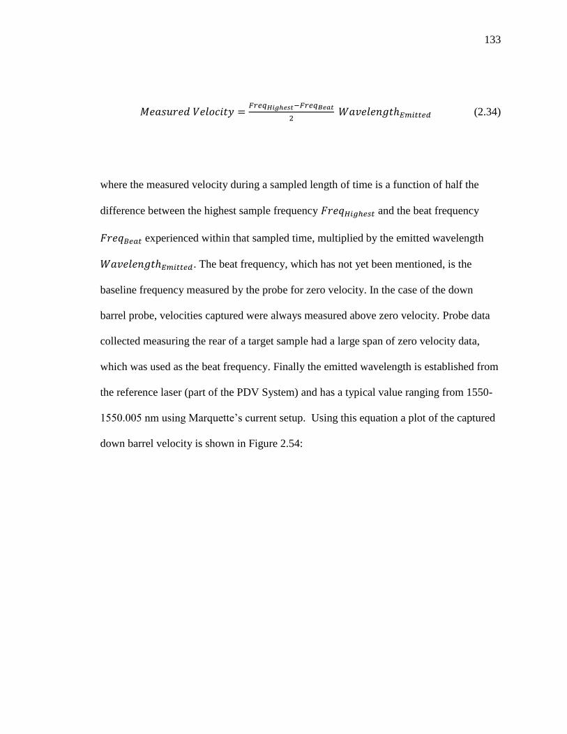
133
𝑀𝑒𝑎𝑠𝑢𝑟𝑒𝑑 𝑉𝑒𝑙𝑜𝑐𝑖𝑡𝑦 =𝐹𝑟𝑒𝑞𝐻𝑖𝑔ℎ𝑒𝑠𝑡−𝐹𝑟𝑒𝑞𝐵𝑒𝑎𝑡
2 𝑊𝑎𝑣𝑒𝑙𝑒𝑛𝑔𝑡ℎ𝐸𝑚𝑖𝑡𝑡𝑒𝑑 (2.34)
where the measured velocity during a sampled length of time is a function of half the
difference between the highest sample frequency 𝐹𝑟𝑒𝑞𝐻𝑖𝑔ℎ𝑒𝑠𝑡 and the beat frequency
𝐹𝑟𝑒𝑞𝐵𝑒𝑎𝑡 experienced within that sampled time, multiplied by the emitted wavelength
𝑊𝑎𝑣𝑒𝑙𝑒𝑛𝑔𝑡ℎ𝐸𝑚𝑖𝑡𝑡𝑒𝑑. The beat frequency, which has not yet been mentioned, is the
baseline frequency measured by the probe for zero velocity. In the case of the down
barrel probe, velocities captured were always measured above zero velocity. Probe data
collected measuring the rear of a target sample had a large span of zero velocity data,
which was used as the beat frequency. Finally the emitted wavelength is established from
the reference laser (part of the PDV System) and has a typical value ranging from 1550-
1550.005 nm using Marquette’s current setup. Using this equation a plot of the captured
down barrel velocity is shown in Figure 2.54:

134
Figure 2.54 Final data collected from the down barrel PDV.
Data between 0 and 500 microseconds captures the velocity of the projectile
traveling down the barrel peaking at a velocity of 197.25 m/s, which compares well with
anticipated light gate measurements mentioned in section 2.2.5. Data after 500
microseconds is no longer valid as the probe has been disrupted. By 550 microseconds,
the probe has been severed from the laser fiber optic line. As anticipated, only the top
0.5% of data seems to show the correct velocity. As more data is included to 2.5%, the
trend of the velocity is still captured, but the spread of velocities increases. By the time
100% of data is included the velocity trend can no longer be seen.
In addition to PDV probes, Dynasen pins can be used to find time of arrival at
direct set points on a target’s surface. This is useful for triggering data collection from the
PDV probes. Alternately, three pins when spaced out over target within the flyer impact
area can return the alignment of flyer and target at impact. Mounting the pins can be
difficult, but after drilling a hole an epoxy specific to the bonded materials plus a weight

135
or clamp keeps the pins from shifting during set time. Pins come in two main types:
piezoelectric pins that when crushed create a voltage spike and make-pins that when
impacted with a conductive material create a circuit.
Figure 2.55 Piezoelectric pin [160].
Figure 2.56 Conductive make-pin [160].
These pins as mentioned in the above figure can be connected to sensing equipment via
purpose built BNC cables also sold by Dynasen. Alternatively, though not recommended
by the manufacturer, once the cables have been used they can and have successfully been
reused by soldering the two wires onto the exposed probe pin end.

136
2.2.7 Vacuum System
Figure 2.57 The Marquette 2 inch gun vacuum system.
Downrange of the barrel, a target and catch tank can be rolled apart to access
specific experimental setups, or vacuum seal prior to firing. While the target tank is used
as the experimental hub for the collision, the vacuum system allows the entire gun
assembly to come to equilibrium pressure with a post firing pressure, below the range of
a single atmosphere. To enable this, both the target and catch tank are vacuumed down to
~60 millitorr pressure at the onset. This keeps the projectile free of any forward pressure
during the shot and allows the shot to be contained within the system. A series of two
137
vacuum gauges shown below in Figure 2.58, allows for monitoring of vacuum pressure
between 0 to -30 in Hg (Dial Gauge) and 2000 to 1 millitorr (KJL Thermocouple [161]).
The dial gauge functions using a bourdon tube, which contracts and expands based on the
pressure within the system actuating the dial. These gauges are the same types that are
often used in high-pressure applications. The thermocouple gauge measures the voltage
across a wire exposed to the pressure within a chamber, based on the pressure molecules
that are able to take more or less heat away from the wire affecting voltage readings. In
general, higher pressures take more heat away and correspond to lower voltages. In
practice, these gauges are often used as controllers, switching rough pumps (used for
viscous or Knudsen flow) like Marquette’s Agilent rotary vane vacuum to finer pumps
like a turbo molecular pump (used for molecular flows) [162].
Two gauges were chosen, as the useful ranges through which they measure
pressure are different. Even though a gauge might be advertised to read down to 0
absolute pressure readings with an error of ±0.5 in Hg (12.7 Torr), the guage would not
be able to resolve the range between 50-100 millitorr used in gas gun experiments. Thus,
a physical gauge allowed for experimenters to physically observe the rough status of
vacuum and pressurization in the tank without the use electrical equipment, in case of
fault. For fine measurements the electrical KJL gauge measured pressures with
manufacturer set points around 100 and 500 millitor, around the region of experimental
interest. An additional benefit of the KJL gauge was the ability to send an electrical
signal to the control system for remote observation of vacuum pressure in the Labview
terminal.

138
Before firing the vacuum safety valve should be closed to isolate the KJL gauge
from sudden pressure shocks occurring during experimentation. After firing is complete,
remaining particulates are scrubbed from the system by forcing air down the barrel and
opening the manual valve to Marquette’s rough vaccum pump, after passing through a
filter.
Figure 2.58 Vacuum gauges: high pressure and low pressure.
A complete assembly of the vacuum system is shown below in Figure 2.59.

139
Figure 2.59 Distribution system reference diagram.
Bringing the system pressure down to a complete vacuum is often difficult with
leaks being hard to both locate and seal. Leaks are to be expected wherever there is a
joint between two separate components, so care in the preparation of components before
mating saves time. Grease should be freshly applied to all separated O-ring seals exposed
to vacuum. Grease has also been applied to NPT threading after pipe tape as well as a
very light coating on KF40 couplings. For positive pressure, applied bubble solution
allows for visual identification of depressurization; however, bubble solution placed on
sections under vacuum also bubbles, but on the inside of the opaque apparatus, which is
not helpful.

140
There are two main methods for detecting vacuum leaks. In situations where the
pressure dwells between both the high and low pressure gauges for longer than
expectation (~1 hour), one should scan the suspect sections by simply listening for leaks.
At the time of this report, only DOW Corning vacuum grease was available for use
within the shock lab. Given a slight size mismatch on the pressure diagnostic, bulkhead
grease applied around the joining collar would slowly be pulled into the system.
When vacuum pressure falls below 2000 millitorr and reaches a steady state such
that the leak rate into the system counteracts the vacuum applied, helium can be utilized
to detect the leak. A wand expelling helium placed near the suspected leak will cause the
pressure to quickly rise because the smaller molecular diameter of helium flows more
quickly through exposed orifices raising the steady state pressure [163]. For a more
controlled application, a plastic bag can easily allow only desired regions of exposure and
conserve helium. In fact, hydrogen could be used with greater effect; however, as
mentioned throughout this and other sections, hydrogen flammability raises concern.
While vacuum grease can be used in all sealing cases, Apiezon Q is a less sticky
and cost effective method of sealing leaks. Apiezon Q has the consistency of a putty, with
an even greater viscosity as compared with grease. When observed on other systems, it
neither dried nor stuck to the hand of the researcher and also remained reusable. Apiezon
Q however is not recommended for sealing O-rings. Dow Corning Vacuum Grease and
Apiezon Q can be sourced from both vacuum suppliers as well as McMaster-Carr. The
complete list of parts that make up the Vacuum System are catalogued within Table 2.15
below.

141
Table 2.15 Vacuum System Callout Table
Callout Part Name Supplier Part Number Notes Inlet Outlet
V1 Gasket McMaster Carr 8516T238 ANSI 2”
V2 Pipe Flange McMaster Carr 44685K16 ANSI 2” pipe 2” FNPT
V3
V4 Schedule 80 Pipe McMaster Carr 46755K65 5” Length 2” MNPT 2” MNPT
V5 Vacuum Safety Valve DuraValve 2” DM340 Rated 1000psig 2” FNPT 2” FNPT
V6 2” Adaptor Ideal Vacuum P106111 2” MNPT KF-40
V7 KF 40 Centering Ring Ideal Vacuum P101962 KF40
V8 KF 40 Clamp Ideal Vacuum P106717 KF40
V9 Dust Filter Kurt J Lesker PFI843KF40B KF40
V10 6-Way Ideal Vacuum P102644 KF40 KF40
V11 Blank Ideal Vacuum P101204 KF40
V12 ¼” Adaptor Ideal Vacuum P101312 KF40 ¼” FNPT
V13 Vacuum Gauge Wika 4253397 ¼” MNPT
V14 1/8” Adaptor Ideal Vacuum P101311 KF 40 1/8” FNPT
V15 Thermocouple Gauge Kurt J Lesker KJL615TC-K 1/8” MNPT
V16 6’ Flex Hose Ideal Vacuum P103808 KF 40 KF 40
V17 Ball Valve Ideal Vacuum P103570 KF 40 KF 40
V18 1’ Flex Hose Ideal Vacuum P103803 KF 40 KF 40
V19 Vacuum Reducer Ideal Vacuum P101230 KF 40 KF 25
V20 KF 25 Centering Ring Ideal Vacuum P101962 KF 25
V21 KF 25 Clamp Ideal Vacuum P106717 KF 25
V22 Vacuum Pump Agilent DS 602 KF 25
V23 Oil Exhaust Filter Agilent 949-9392 KF 25 KF 25
2.2.8 Some Notes on Machining
In the experimental realm of shock physics, preparation work and machining will
take the lion share of work time. It is assumed here that the reader already has both the
knowledge and skills to design and draft, that is to say make-up the dimensions for
sculpting a part from a blank piece of material.

142
Figure 2.60 Marquette machine shop.
During this study all of the machines within Marquette’s machine shop, shown
above, were utilized. While not perfect for every task, each of the tools within the shop
were, when taken collectively, enough to perform experiments within an acceptable
tolerance (in most cases down to a few thousandths accuracy). There are always more
ways to complete a given machining task and the number of options increases with the
number or tools available.
A significant portion of time in the design and manufacture of experiments will be
spent in the design and machining of the targets and mounts to the highest degree of
accuracy possible, while also making sure to accomplish tasks in a timely fashion and
with care not to damage the machining equipment. In general, this can be accomplished
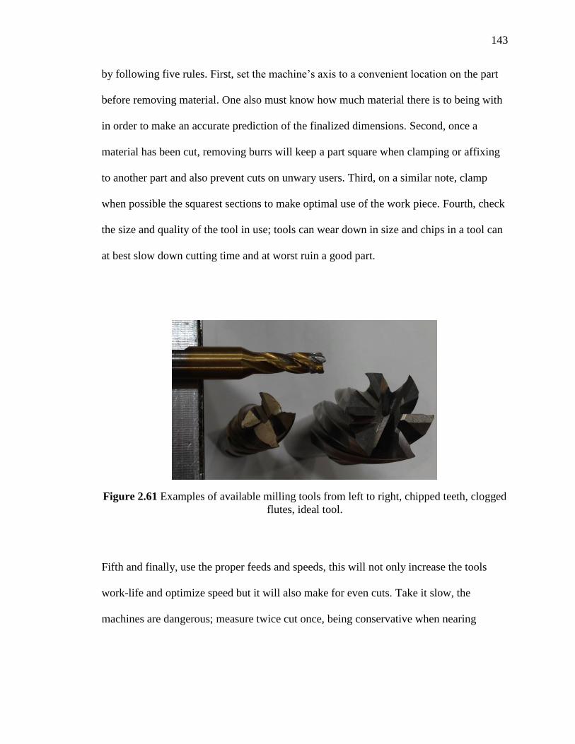
143
by following five rules. First, set the machine’s axis to a convenient location on the part
before removing material. One also must know how much material there is to being with
in order to make an accurate prediction of the finalized dimensions. Second, once a
material has been cut, removing burrs will keep a part square when clamping or affixing
to another part and also prevent cuts on unwary users. Third, on a similar note, clamp
when possible the squarest sections to make optimal use of the work piece. Fourth, check
the size and quality of the tool in use; tools can wear down in size and chips in a tool can
at best slow down cutting time and at worst ruin a good part.
Figure 2.61 Examples of available milling tools from left to right, chipped teeth, clogged
flutes, ideal tool.
Fifth and finally, use the proper feeds and speeds, this will not only increase the tools
work-life and optimize speed but it will also make for even cuts. Take it slow, the
machines are dangerous; measure twice cut once, being conservative when nearing
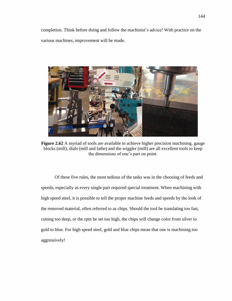
144
completion. Think before doing and follow the machinist’s advice! With practice on the
various machines, improvement will be made.
Figure 2.62 A myriad of tools are available to achieve higher precision machining. gauge
blocks (mill), dials (mill and lathe) and the wiggler (mill) are all excellent tools to keep
the dimensions of one’s part on point.
Of these five rules, the most tedious of the tasks was in the choosing of feeds and
speeds, especially as every single part required special treatment. When machining with
high speed steel, it is possible to tell the proper machine feeds and speeds by the look of
the removed material, often referred to as chips. Should the tool be translating too fast,
cutting too deep, or the rpm be set too high, the chips will change color from silver to
gold to blue. For high speed steel, gold and blue chips mean that one is machining too
aggressively!

145
Figure 2.63 Steel chips from left to right: blue, silver, and gold.
Unfortunately for other commonly machined materials, such as polycarbonate,
brass, wood and aluminum, and when using carbide tooling, the method for noticing the
proper machine settings are not as easily noticed. Choosing improper settings with other
tooling and material will often be heard or felt and, if not immediately stopped, will often
damage the cutting tool.
Therefore, before beginning any job in the shop one should have a rough idea of
the cutting speeds and feeds to use. To make it simple, the equation below is suggested to
be used for lathing, milling, and only in the hobbyist setting. This is meant to be a
simplified version for a quick calculation before turning on the machine. For large
material runs, where tool wear and time per part are more valuable, consult the
Machinists handbook [164] or textbook on machining! For the mill and drill press, one
should use the below equation where N is the Spindle rpm, V is the feed in ft/min, Ff and
Fd are the feed and depth factor (.8), and D tool diameter (or part diameter for the lathe)
in inches:

146
𝑁 =12 𝑉 𝐹f F𝑑
𝜋 𝐷≈
4 𝑉
𝐷 (2.35)
The equation above, when combined with the values in Table 2.16 below, and
typical lower feed rate utilized when hand machining, are generally good as ballpark
estimates for the speeds to run mill, drill press and lathe using high speed steel bits. For
carbide bits one can general increase rpm by 2-3 times. For hole diameters less than an
1/8 inch, it is recommended to add lubrication to the drill bit and pay extra close attention
to prevent chips from clogging up the flutes, which are the only path of exit during
drilling. On the mill finishing pass, one should take off a lesser amount of material,
decrease the feed rate and increase the rpm for the best possible finish (if looks or flatness
is important).
Table 2.16 A crude Feed Rate Table for Common Items (for more precise numbers,
please consult the Machinist’s Handbook [164])
Material Approximate Material Feed
Rate HHS (choose average or adjust
to lower for harder material variant) Recommendations
Titanium 70-110 ft/min Carbide Tooling
Ferritic and
Austenitic Stainless
Steel
25-75 ft/min Carbide Tooling
Low Carbon Steel 65-110 ft/min Carbide Tooling
Medium Carbon
Steel 25-100 ft/min Carbide Tooling
Copper Alloys 100-350 ft/min High Speed Steel
and Dull the Cutter
Aluminum 350-600 ft/min Two Flute High Speed Steel
Polycarbonate 350-1000 ft/min High Speed Steel Some resultant RPM will max out the mill lathe and drill press, use highest comfortable setting.

147
Identifying the difference between high speed steel and carbide is a simple matter.
In general, carbide bits are both heavier than their counterparts for a given size. For mill
bits, a gold coating is added while high speed steel bits remain silver. Lathing tools made
from carbide are often pre-shaped and mounted within steel, while high speed steel tools
are the same material throughout.
Other materials such as plastic, wood, and rubber within this study were cut
utilizing the epilog engraver, scroll saw, chop saw, and band saw. While all but the epilog
engraver were not great for precision cutting, these machines were all clearly labeled for
operation.
3. EXPERIMENTAL SETUP
Each experiment will be different, though it will use the same common elements
within each shot: the gun, diagnostic equipment and samples. Each of these elements has
the ability to cause harm to operators and to others: high pressure gases, high velocity
projectiles, laser light capable of harming optical tissue and pulmonological hazards such
as fine particulates, like silica. Each of these common items is addressed in the protocol
outlined below to provide a safe, repeatable standard operation procedure relevant to
most gas gun experiments and basic record of past experiments.

148
3.1 Firing Procedure and Safety Protocol
Standard Operating Procedure (SOP) – June 10, 2017 Edition
Marquette University
Setup Procedure for Two-Inch Gas Gun
The following is to be used in conjunction with the PDV Standard Operating Procedure.
Date: ______/ /________
Preliminary Information
1.__ Schedule shot with the MARVL visualization lab.
2.__ Record pre-shot data:
Sponsor/Grant: ____________________________
Experiment Designer(s): __________________________________
Please attach a CAD drawing or relevant simulation if applicable!
Type: Basic Schematic:
o Flyer Plate
o Reverse Ballistic
o Pressure Shear
o Conical
o Other: _____________
Brief Description:
______________________________________________________
______________________________________________________
______________________________________________________
______________________________________________________
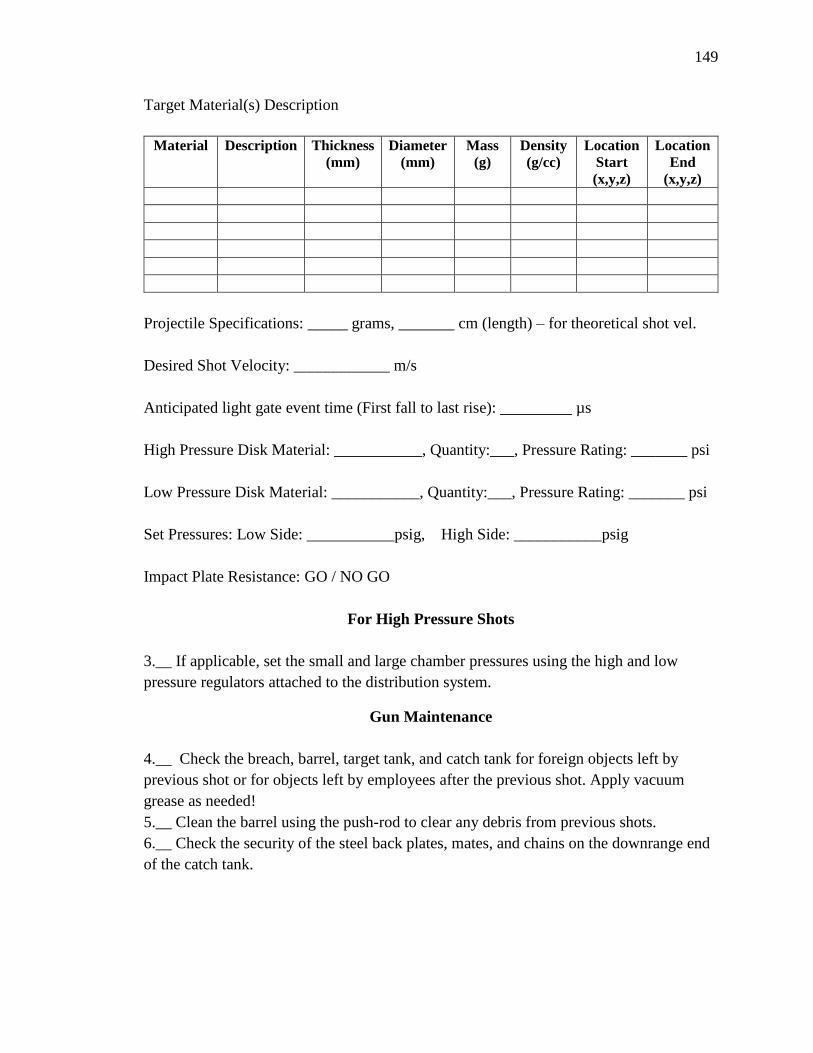
149
Target Material(s) Description
Material Description Thickness
(mm)
Diameter
(mm)
Mass
(g)
Density
(g/cc)
Location
Start
(x,y,z)
Location
End
(x,y,z)
Projectile Specifications: _____ grams, _______ cm (length) – for theoretical shot vel.
Desired Shot Velocity: ____________ m/s
Anticipated light gate event time (First fall to last rise): _________ µs
High Pressure Disk Material: ___________, Quantity:___, Pressure Rating: _______ psi
Low Pressure Disk Material: ___________, Quantity:___, Pressure Rating: _______ psi
Set Pressures: Low Side: ___________psig, High Side: ___________psig
Impact Plate Resistance: GO / NO GO
For High Pressure Shots
3.__ If applicable, set the small and large chamber pressures using the high and low
pressure regulators attached to the distribution system.
Gun Maintenance
4.__ Check the breach, barrel, target tank, and catch tank for foreign objects left by
previous shot or for objects left by employees after the previous shot. Apply vacuum
grease as needed!
5.__ Clean the barrel using the push-rod to clear any debris from previous shots.
6.__ Check the security of the steel back plates, mates, and chains on the downrange end
of the catch tank.

150
Target Setup: Velocity Laser Block
7.__ Orient the velocity blocks, lasers and collimators on the velocity plate, aligning the
collimators to pick up a ~5 Volt signal. Make sure that all screws are properly attached.
Place the velocity block setup into the target tank and recheck the four channels recording
peak velocity, the ability of the beams to be broken, and the relation between the
channels and their location within the velocity block path. (Velocity Pin 1 is closest to the
muzzle; pins increasing in number increase in distance away from the first pins by a
nominal distance of 0.75 inches for each subsequent pin,)
Final Velocity Recordings (Pre-Vacuum)
Velocity Pin 1 Voltage DC Offset _____
Velocity Pin 2 Voltage DC Offset _____
Velocity Pin 3 Voltage DC Offset _____
Velocity Pin 4 Voltage DC Offset ______
Trigger Level: ________, Trigger Time: ___________, Trigger Channel __________,
Time Divisions:_____________ microsec/div
Channel 1 2 3 4
mV/div
impedance
Target Setup: Target Plate Orientation
8.__ Attach the target plate to the three mounting bolts and use the radial surface dial to
check radial symmetry. The alignment should in general be less than a milli-radian in
offset. If target plate is already attached, recheck alignment.
Alignment: ___________________ milli-radians
Target Setup: PDV Settings
9.__ Ensure Laser/High Pressure warnings signs are on the door.
10.__ Ensure PDV probes and PZT/shorting pins are epoxied into the target ensure PDV
are within the acceptable range of light return (better than -30dBm).
11.__ Take a picture of the target prior to assembly onto the holder.
12.__ Place the target into the target holder. Wear protective mask and eyewear if
necessary.

151
13.__ In the case of pressure-shear/conical shots, align blank projectile, placed in the
muzzle of the barrel, to the target fixture ensuring angles mate. Afterwards, remove blank
projectile.
14.__ Take an additional picture of final assembled target and attach.
15.__ Measure the distance between the target and the end of the barrel. Record this
value. Try to minimize or eliminate free flight.
16.__ Check responsivity/light return of PDV probes again.
17.__ Feed PDV probes out of the hermetic bulkhead and connect to the patch cables
leading into the system. LABEL patch cables corresponding to probe placement.
a) Probe #1 – Placement___________________ - Channel #__________
b) Probe #2 – Placement___________________ -Channel #__________
c) Probe #3 – Placement___________________ - Channel #__________
d) Probe #4 – Placement___________________ - Channel #__________
18.__ Recheck the light return on the PDV and the functionality of the velocity block:
Target Laser Wavelength: ________ (nm)
Reference Laser Wavelength: ________ (nm)
Expected Base Beat Frequency: _____________ (GHz, theory)
Measured Sample Frequency: _______________ (GHz, experimental)
Booster Laser Power: ___________ mA
1 - Target Power: _____________ (dBm), Combined Power: __________ (dBm)
2 - Target Power: _____________ (dBm), Combined Power: __________ (dBm)
3 - Target Power: _____________ (dBm), Combined Power: __________ (dBm)
4 - Target Power: _____________ (dBm), Combined Power: __________ (dBm)
Trigger Source: _____________________ (1, 2, 3, 4, or external)
Trigger Level: _____________________, Trigger Time: ______________________
Time Divisions:_____________microsec/div
Channel 1 2 3 4
mV/div
impedance

152
19. Terminate emission of PDV until later checks.
Target Setup: PZT/Shorting Pins Settings
20. ___ Connect PZT/shorting pins. LABEL placement.
a) Pin #1 – Placement___________________ - Channel #__________ - Type:_____
b) Pin #2 – Placement___________________ - Channel #__________ - Type:_____
c) Pin #3 – Placement___________________ - Channel #__________ - Type:_____
d) Pin #4 – Placement___________________ - Channel #__________ - Type:_____
Trigger Source: _____________________ (Summation/Direct from Channel #)
Trigger Level: ______________________, Trigger Time: _________________________
(Recommended less than 500 mV trigger threshold for PZT pins)
Time Divisions:_____________microsec/div
Recommendations:
a) Set scope to 5 V/div, 500 ns/div.
b) Use the “EXT OUT” from the Dynessen to the external trigger “EXT TRIG IN” on
the PDV scope.
c) Impedance SHOULD BE 1 Mohm
d) DC Offset SHOULD BE THE SAME FOR ALL CHANNELS:
Channel 1 2 3 4
mV/div
impedance
External Trigger Sent to: ________________________
2. ___ Test Trigger setup between summation circuit, pin scope, and PDV scope.
a) Set the trigger.
b) Perform battery test of each BNC cable with a trigger at less than 150mV.
c) Set posttest triggers to <500 mV for actual PZT pins.
d) Place each signal at zero offset.
e) Trigger the delay 2 µs to the left of center.
3.__ Once satisfied with target alignment and in-target diagnostics, slide the blast shield
into place.
4.__ Recheck light return for PDV, and triggering once blast shield is in place.
Vacuum Process
5.__ Place the large O-ring between the catch tank and target tank, lubricate if needed.
6.__ Re-check that all non-essential items are taken out of the target tank and catch tank.

153
7.__ Close the vacuum tank and attach all eight bolts coupling the target tank and catch
tank.
8. ___Close the catch tank man-way and use all eight bolts to secure the hatch.
9.___Close the breach with burst disks making sure that all 6 O-rings are in place and
undamaged.
10.___Note the ideal reservoir tank burst disk pressure and trigger tank burst disk
pressure on the data sheet (should have been previously recorded).
11.__ Make sure that all ports and the barrel are locked down, especially PDV bulk-head
and Breach Tank.
12.__ Check that air hose is connected to the Haskel pump on the high pressure side of
the system.
13.__ Turn on Labview and the NI Daq Chassis before checking functionality and
beginning pull-down.
•__ Open the vacuum safety valve.
•__ Open the building vacuum valve.
•__ Once the system has reached a pressure of -20inHg close the building
vacuum valve.
•__ Turn on the Agilent pump.
•__ Open valves 1-4 on the pressure side.
•__ Run the Haskel.
•__ Stop Haskel.
•__ Close valves 1-4.
14.__Test the seals within the breach using low pressure air, before releasing this air
pressure.
15.__ Ensure that air within the large and small chambers is released and is not under
pressure during put down. In addition, make sure that all high pressure valves are closed.
16.__ Send out a warning to adjacent labs that a pressurization will commence within the
next two hours, corresponding with previously schedule time.
17.__ Run the Agilent to the desired millitorr range.
Prior to Pressurization
18.__ Perform a final recheck on all diagnostic systems, and record any changes:
a)__ PDV Light Return
b)__ PZT/Shorting Pin Triggering Circuit
c)__ Laser Velocity Setup
19.__ Record the final vacuum pressure on the data sheet.
20.__ Setup computers with Skype or FaceTime to record the pressure gauges and
oscilloscopes.
21.__ Evacuate non-essential personnel and alert nearby labs of impending test.

154
22.__ Ensure scope settings have been recorded.
23.__ Arm oscilloscopes to be triggered.
24.__ Engage lasers so that PDV probes are emitting light.
25.__ Capture preliminary data on PDV scope to establish pre-shot beat frequency, if any
measurements greater than 1 millisecond are being made.
26.__ Perform final checks – begin firing procedure only after PDV check and setup
check are complete.
27.__ Ensure that at least one pair of laser safety goggles has been placed outside of EH
040 for use after the shot.
28.__ Perform a personnel sweep of the room to ensure no persons are in the room.
29.__ Check Room EH 028 and EH 028a to insure no personnel are in the room.
30.__ Post personnel at either end of the hall to ensure that there will be no persons in the
hallway during the shot.
PROCEED TO NEXT PAGE FOR FIRING INSTRUCTIONS

155
Firing Procedure for Two Inch Gas Gun
To shoot the two-inch gun. The safety procedure includes the following checks:
1.__ Acquire final approval
Signatures for Shot Approval:
Lab Supervisor
Print:
_______________________________________________________________________
Sign:
________________________________________________________________________
Experiment Lead
Print:
_______________________________________________________________________
Sign:
________________________________________________________________________
Gun Personnel Information (Important):
Projectile Specifications: ______grams, ________cm (length) – for theoretical shot vel.
Anticipated Shot Velocity: ____________m/s
High Pressure Disk Material: ____________, Quantity:___, Pressure Rating: _______psi
Low Pressure Disk Material: ____________, Quantity:___, Pressure Rating: _______psi
Set Pressures: Low Side: ___________psig, High Side: ___________psig
2.__ Gun personnel execute the following steps remotely. Understand that during this
stage the gun may fire!!!
a.__ Open Haskel pump valve to pressurize both sections of the breach.
b.__ Once the low pressure is reached, close the low pressure chamber.
Final Low Pressure Pre Creep: _________psig,
c.__ Once the pressure within the breach exceeds low side set pressure, close the
vacuum safety valve!
Final Lowest Vacuum Pressure: _________psig,
d.__ Once high pressure chamber within the breech reaches target pressure, close
the high pressure breach.
Final Low Pressure: _________psig, High Pressure: _________psig
e.__ Signal experimenters that the gun is ready to fire. Give count and release the
small chamber.
f.__ Do Not! begin to ventilate and re-pressurize the vacuum system.
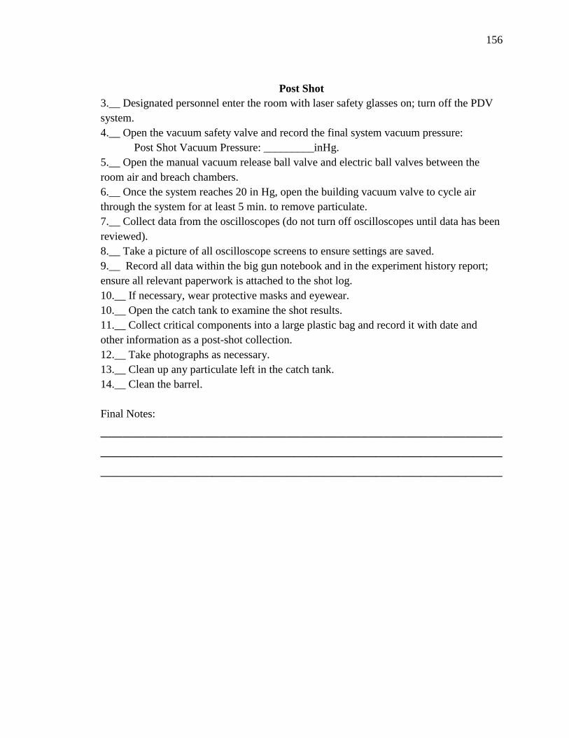
156
Post Shot
3.__ Designated personnel enter the room with laser safety glasses on; turn off the PDV
system.
4.__ Open the vacuum safety valve and record the final system vacuum pressure:
Post Shot Vacuum Pressure: _________inHg.
5.__ Open the manual vacuum release ball valve and electric ball valves between the
room air and breach chambers.
6.__ Once the system reaches 20 in Hg, open the building vacuum valve to cycle air
through the system for at least 5 min. to remove particulate.
7.__ Collect data from the oscilloscopes (do not turn off oscilloscopes until data has been
reviewed).
8.__ Take a picture of all oscilloscope screens to ensure settings are saved.
9.__ Record all data within the big gun notebook and in the experiment history report;
ensure all relevant paperwork is attached to the shot log.
10.__ If necessary, wear protective masks and eyewear.
10.__ Open the catch tank to examine the shot results.
11.__ Collect critical components into a large plastic bag and record it with date and
other information as a post-shot collection.
12.__ Take photographs as necessary.
13.__ Clean up any particulate left in the catch tank.
14.__ Clean the barrel.
Final Notes:
______________________________________________________
______________________________________________________
______________________________________________________

157
4. THEORETICAL VS. EXPERIMENTAL GUN BEHAVIOR
4.1 Breach Charging Time
In order to reach pressures above either shop air or the nitrogen supply tank, a
Haskel pressure booster is utilized. In practice, one could derive the pump curve with the
performance curve Figure 4.1, in additional to the inlet condition and losses from the
various components. This is beyond the scope of this paper, as all components leading
from the Haskel to the breach were chosen to meet safety requirements; finding
components that were both compatible and operated at high-pressure greatly limited
availability of choices.
Figure 4.1 Performance curve for the AGT-62/152H Haskel Pressure Booster [165]. PS
is the gas supply pressure (psig), Pa is the driving pressure (psig), Po is the outlet pressure
(psig), and QA is the gas flow of the outlet gas (SCFM).

158
Optimization of the pressurization system mainly focused on reducing numbers of
bends and choosing the largest possible flow area. Looking at the pump curve, one finds
the range of pressure supply, PS, to the system ranges from 500-2,500 psig, within these
ranges a final breach pressure of 10,000 psig is attainable. While testing it was noted that
the Haskel was able to operate with the shop air supplied by the building. By assuming a
linear relation between pressure supply and final outlet pressure, it also appears that the
Haskel would be capable of pressurizing the breach to ~14,000 psig simply with the shop
air supply pressure of 100 psig. Given the flattening of the curves in Figure 4.1 it was
anticipated that pressurized air to the breach using shop air supply while slow would have
a relatively constant flow rate and result in a linear increase in breach pressure over time.
Recalling the control section of this report (2.2.1), one might recall mention of a
needle valve regulating flow from the shop into the Haskel (Figure 2.34). While this
served as an interim control device, it was eventually swapped out in favor of solenoid
valve, which is less restrictive and effectively increases flow from the shop to the Haskel.
In Figure 4.2, the pressurization of the breach for various driving conditions, under shop
air supply and driving gas are shown.

159
Figure 4.2 Pressurization curve of the combined small and large chamber volume within
the breach for different flow control valves to the Haskel drive air supply.
As can clearly be seen, the flow of air to the Haskel is least impeded by the
solenoid valve. With this configuration, an extremely linear rise in pressure within the
breach is observed with respect to time. Reviewing Figure 4.1, one will note that a supply
pressure of 100 psig is not presented; the lowest supply pressure of 500 psig has a near
linear pump flow rate out to 3,000 psig. Comparing Figure 4.2 with the trend in Figure
4.1, one can anticipate that the effect of reduced flow rate would be less noticeable as
compared with higher supply pressures, though this may reduce pump performance at
higher outlet pressures (making the linear fit over estimate performance) and increase
pumping times.
A rough estimate of pressurization time using the shop air supply was conducted
to evaluate the need of a nitrogen tank for high-pressure shots. It is assumed that the
volume filled comprises the entire breach (both high and low side chambers), as the small

160
chamber comprises a volume significantly smaller volume than that of the high side
chamber. Assuming the pressure continues to increase linearly, one can conclude that the
time to reach a set pressure given supply pressure of 100 psig to is given by the equation:
𝑡 =𝑃𝑓
0.5 (4.1)
where t is the total pressurization time in (seconds), Pf is the final set pressure, within the
entire breach (in psig), and 0.4867 (psi/s) is the rate of pressurization found observed in
Figure 4.2 above. This assuming the pressurization does not slow, the total time to
pressurize to a 10,000 psig shot, using shop air, is ~5.56 hours. This is why for shots
above 1000 psig, which take just over a half-hour, researchers should seriously consider
use of the nitrogen tank!
4.2 Burst Disk Failure
In order to release the gases, within the breach, the dual diaphragm system relies
on the mechanical failure properties of materials such as: mylar, aluminum, bronze
copper and steel. These round plates of material, known as burst disks, fit between
pressure chambers within the breach assembly. When these disks are stressed beyond
yield strength, they fail, petaling open and releasing driving gases into the gun barrel.

161
While most burst disks are supplied by Physics Applications Inc. with burst
pressure ranges pre-labeled (determined by experimental pressure testing) they are
expensive, $50-$100 a shot, and had high failure pressure (1297 psi minimum). Lower
pressures were needed to fire at velocities for pressure shear and burst disks produced at
Marquette promised lower cost per shot. In this author’s experience developing new
firing methods for Marquette’s smaller ¼ gas gun, the fast acting valve was
supplemented with mylar disks cut from sheets, often used as the transparency sheets for
light projectors. Using this same material, larger unscored disks were created and
pressurized until failure, the results of which are shown later in Figure 4.9. Selections of
burst disks are shown below in Figure 4.3.
Figure 4.3 Burst disks in varying states of failure; note the bulging effect of the bronze
disk, which changes the internal volumes of both chambers.
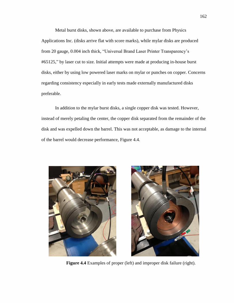
162
Metal burst disks, shown above, are available to purchase from Physics
Applications Inc. (disks arrive flat with score marks), while mylar disks are produced
from 20 gauge, 0.004 inch thick, “Universal Brand Laser Printer Transparency’s
#65125,” by laser cut to size. Initial attempts were made at producing in-house burst
disks, either by using low powered laser marks on mylar or punches on copper. Concerns
regarding consistency especially in early tests made externally manufactured disks
preferable.
In addition to the mylar burst disks, a single copper disk was tested. However,
instead of merely petaling the center, the copper disk separated from the remainder of the
disk and was expelled down the barrel. This was not acceptable, as damage to the internal
of the barrel would decrease performance, Figure 4.4.
Figure 4.4 Examples of proper (left) and improper disk failure (right).
163
Before each shot, it is of utmost importance to choose burst that will fail in a
controllable manner. In order to aid discussion, the disk between the small chamber and
gun barrel shall be referred to as the “low pressure disk” and the disk between the small
chamber and the large chamber as the “high pressure disk” (see Figure 2.7).
To create a method for choosing burst disks, one must make and follow rules. As
mentioned above burst disk come with a pre-labled range of burst pressure; therefore, this
section will assume that the nominal value or range of burst pressure values are known a-
priori. With this in mind, the most important rule is that the gun, if it fires, should always
fire in the correct direction and not backfire into the breach. To ensure this, the low
pressure disk must always be either of the same failure pressure, or lower than the high
pressure disk, else the gun would only be able to function properly as a typical single disk
system, or at worst backfire.
From here, one can begin with the investigation of a burst disk system utilizing a
pair of 0.125 inch thick (nominal) scored aluminum burst disks, with nominal burst
pressure of 1538 psi (this is an average of the minimum and maximum burst pressures
provided by Physics Applications Inc.). This system, with chosen burst disk, has two
degrees of freedom: the small and large chamber set pressure. In order to fire the gun,
pressures within the large chamber must exceed the failure pressure of the high-pressure
disk, while at the same time, the low-pressure disk must never exceed the burst pressure
of the high pressure disk. Remember that burst disks fail by an excess in differential
pressure. By pressuring the small chamber to a set value (up to the low-pressure burst

164
disk burst pressure), one can also raise the pressure within the large chamber to the same
value plus the burst pressure of the high-pressure disk (Note that Pabs ≈ 0 downstream of
the breach). In order to assist with the understanding of this, a diagram displaying the
range of stable operational pressure set points is included in Figure 4.5 below.
Figure 4.5 Range of theoretical set pressures for a 0.125 Alum-Alum burst disk
configuration using nominal burst pressure.
Unfortunately, burst disks do not fire at a set pressure, but rather a range of
pressures. Disks provided by Physics Applications Inc. are provided with both a high and
low pressure burst value. Additionally, effects such as creep, mentioned in section 2.2.4,
mean that factors of safety around all three bounds are needed, further limiting the stable
ranges of operation.

165
To prevent the first disk from firing, the pressure difference across the gun barrel
and small chamber must be less than the minimum burst pressure of the disk. To ensure
this, the chamber should be set at a pressure 85% of the minimum burst disk pressure, the
first of three boundary conditions. This safety factor underestimates the burst disk
strength at low pressures and allows for pressure creep as the high pressure burst disk,
under higher pressures, deforms into the small chamber cavity. This factor may need to
be lowered especially for low-pressure burst disks, as creep has a much larger effect
relative to the burst pressure of the disk. To calculate the small chamber set pressure, the
following equation is proposed:
SmChamber𝑃𝑟𝑒𝑠𝑚𝑎𝑥 = 0.85 (𝐷𝑖𝑠𝑘𝐿𝑃𝑚𝑖𝑛) (4.2)
where SmChamber𝑃𝑟𝑒𝑠𝑚𝑎𝑥 is the set pressure of the small chamber and 𝐷𝑖𝑠𝑘𝐿𝑃𝑚𝑖𝑛 is the
minimum know burst pressure of the low pressure disk.
To this point, it is has been expected that the minimum and maximum burst
pressures are well characterized; this cannot be assumed. Therefore, ranges restricting
maximum and minimum large chamber pressure are chosen to ensure the gun fires when
desired and does not fire under other circumstances. The large chamber is therefore
restricted to pressures between 80% and 20%, bounding the experimental use between
the extreme combinations of burst disk failure and non-failure. It should be noted that the
85%, 80%, and 20% values are arbitrarily chosen to afford extra allowance to the
manufacturer or laboratory quoted burst pressure range. These factors may need to be

166
adjusted as preloading loading disks to test the seal of the breach, temperature of the
breach or conditions in which the disks are kept will affect burst pressure. Based on these
considerations equations with initial safety factors are presented below:
LgChamber𝑚𝑖𝑛𝑃𝑟𝑒𝑠 = 𝐻𝑃𝐷𝑖𝑠𝑘𝑚𝑎𝑥𝑏𝑢𝑟𝑠𝑡 +
(0.2 (2 𝐻𝑃𝐷𝑖𝑠𝑘𝑚𝑖𝑛𝑏𝑢𝑟𝑠𝑡 − 𝐻𝑃𝐷𝑖𝑠𝑘𝑚𝑎𝑥𝑏𝑢𝑟𝑠𝑡)) (4.3)
LgChamber𝑚𝑎𝑥𝑃𝑟𝑒𝑠 = SmChamber𝑃𝑟𝑒𝑠𝑚𝑎𝑥 − 𝐻𝑃𝐷𝑖𝑠𝑘𝑚𝑎𝑥𝑏𝑢𝑟𝑠𝑡 + LgChamber𝑚𝑖𝑛𝑃𝑟𝑒𝑠
+(0.8 (2 𝐻𝑃𝐷𝑖𝑠𝑘𝑚𝑖𝑛𝑏𝑢𝑟𝑠𝑡 − LgChamber𝑚𝑖𝑛𝑃𝑟𝑒𝑠)) (4.4)
where LgChamber𝑚𝑖𝑛𝑃𝑟𝑒𝑠 and LgChamber𝑚𝑎𝑥𝑃𝑟𝑒𝑠 are the acceptable range of large
chamber pressure, 𝐻𝑃𝐷𝑖𝑠𝑘𝑚𝑖𝑛𝑏𝑢𝑟𝑠𝑡 and 𝐻𝑃𝐷𝑖𝑠𝑘𝑚𝑎𝑥𝑏𝑢𝑟𝑠𝑡 are the quoted range of
pressures at which the high pressure disk will burst and SmChamber𝑃𝑟𝑒𝑠𝑚𝑎𝑥 is the
maximum pressure within the small chamber.
The three equations, (4.2) (4.3) (4.4), bound our available pressure settings given
a set of burst disks. To better showcase the utility of these equations, a brief example is
given. For this example, a set of 0.125 inch thick scored aluminum disks with a burst
range of 1297-1779 psi, is considered. From this information, one computes the sample
space shown below in Figure 4.6.

167
Figure 4.6 Plot for the effective working range of 0.125 inch Alum – 0.125 inch Alum
burst disk configuration including a 9 Ply Mylar – 0.125 inch Alum burst disk
configuration.
In the figure, the outer triangle space shows the stated limits of the burst disk as a
function of small chamber pressure. Adding in safety afforded by the 20% and 80%
offsets, one arrives at the final range of high and low chamber pressure settings for the
aluminum disks. If running at a lower breach pressure, one could also use a system
consisting of a low pressure disk made of 9 bonded mylar disks and a high pressure disk
of 0.125 inch Aluminum to save in shot costs. Consideration of cost is unnecessary as the
sample space for the dual aluminum setup includes the same sample space. A list of
available burst disks with usable sample spaces is shown below in Table 4.1. Burst
pressure data for mylar was taken from in-house testing, while metal disk burst pressures
were taken from Physics Applications Inc. values quoted on disks. The author
recommends that for least likelihood of failure the minimum large chamber pressure is
used. Caution should be taken with mylar burst disks, especially at lower pressures as
burst values have been recovered from single tests with an unknown range of burst
pressure!

168
Table 4.1 Compiled List of Available Paired Disk Set Pressures
Setup
Minimum
Low Burst
Pressure
(psi)
Minimum
High
Burst
Pressure
(psi)
Maximum
High
Burst
Pressure
(psi)
Small
Chamber
Maximum
Set
Pressure
(psig)
Minimum
Percent
Above
Burst
Maximum
Percent
Above
Burst
Large
Chamber
Minimum
Pressure
(psig)
Large
Chamber
Maximum
Pressure
(psig)
Minimum
Over
Pressure
Maximum
Over
Pressure
1 Mylar 100 100 100 85 20% 80% 120 169 120.0% 169.0%
2 Mylar 300 300 300 255 20% 80% 360 507 120.0% 169.0%
3 Mylar 450 450 450 382.5 20% 80% 540 760.5 120.0% 169.0%
4 Mylar 525 525 525 446.25 20% 80% 630 887.25 120.0% 169.0%
5 Mylar 600 600 600 510 20% 80% 720 1014 120.0% 169.0%
7 Mylar 800 800 800 680 20% 80% 960 1352 120.0% 169.0%
9 Mylar 1000 1000 1000 850 20% 80% 1200 1690 120.0% 169.0%
9 Mylar
and 0.125
inch
Thick Alum
1000 1297 1779 850 20% 80% 1942 2016.6 109.2% 155.5%
0.125
inch Thick
Alum
1297 1297 1779 1102.45 20% 80% 1942 2269.05 109.2% 174.9%
0.05
inch
Brass
Low
2195 2195 3010 1865.75 20% 80% 3286 3839.95 109.2% 174.9%
0.05
inch
Brass High
3055 3055 4189 2596.75 20% 80% 4573.2 5344.39 109.2% 174.9%
0.063 inch
Brass
Low
3671 3671 5032 3120.35 20% 80% 5494 6421.75 109.2% 174.9%
0.063
inch Brass
High
5441 5441 7460 4624.85 20% 80% 8144.4 9518.33 109.2% 174.9%
.09 inch
Brass 7565 7565 10371 6430.25 20% 80% 11322.8 13233.81 109.2% 174.9%
It was mentioned above that the burst disks within the lab were either purchased
with a pre-labeled range of burst pressures or created and tested in lab. Investigating
further, it was found that most burst disks were created then tested or modeled within a
169
Finite Elements package such as ANSYS before manufacture. Analytically, the design
space for burst disks, both with and without grooves, was limited to one notable mention
within Henri Bernier’s work [167]:
𝑝 =𝐴
1+3.75(𝜀 𝑒⁄ )3𝑒
32⁄ (𝜀 𝑒⁄ )−
1
2 (4.5)
where 𝜀 is groove thickness, e is the burst disk thickness, and p is pressure. However, the
formula within this work is incomplete, as the variable A is left as an open variable
describing “diaphragm dimensions, the depth of the groove and material properties.”
Further investigation into the origins of this formula lead to a paper by JJ Rast [169].
In his paper, Rast includes a formulas for hemispherical disks:
𝑃𝑏𝑢𝑟𝑠𝑡 = 2𝜎𝑢𝑙𝑡 𝑑
𝑎 (4.6)
Where the burst pressure 𝑃𝑏𝑢𝑟𝑠𝑡, is a function of 𝜎𝑢𝑙𝑡the ultimate strength of the
diaphragm, d is the material left at the bottom of the groove, and a is the radius of the
unsupported disk area. Though equations expressing burst pressures in flat round disks
could not be found, though data for scored and unscored flat disks is included in Figure
4.7 below.
170
a) Burst Pressure vs. Thickness Ratio for Flat and Hemispherical disks without scores
b) Burst pressure vs. thickness ratio for flat scored disks
Figure 4.7 Plot of burst pressure vs thickness ratio for various stainless steel 304 and 305
round burst disks. This where P is the burst pressure, E is the modulus of elasticity, t is
the disk thickness, r is the diaphragm bend radius, a is the radius of the unsupported disk
area, d is the material left at the bottom of the groove, 𝝈𝒖𝒍𝒕 is the ultimate strength of the
diaphragm, 𝝈𝒂𝒖 is the apparent strength of the diaphragm, 𝝐𝒖𝒍𝒕 is the ultimate strain, and
𝝐𝒂𝒖 is the apparent ultimate strain.
171
While the above curves does account for some disk relevant dimensions and
Elastic Modulus, it does not apply to disks made of materials available to the lab. Aside
from these sources, references for burst disk pressure, both with and without cut grooves,
were not found. As mentioned before, forums recommend simulation packages, such as
ANSYS, or characterizing burst pressure through experiment. Therefore, a quick formula
for mylar has been proposed and derived below, assuming thin sheet disks with fixed
boundaries around their circumference.
First, the failure of the mylar disk will be assumed to be similar to a spherical
tank, with internal pressure shown in Figure 4.8. This was a valid assumption as
experimental results for mylar show that material deformation before failure was
approximately hemispherical in shape. This was not the case for metal disks which were
found to have much lesser deformation before burst.
Figure 4.8 Burst disk failure approximation.

172
Beginning with a force balance, it is assumed that the pressure applied over the projected
area of the internal sphere wall will balance with the materials strength exerted along the
diameter of the sphere.
𝑃𝑏𝑢𝑟𝑠𝑡(𝜋𝑟𝑖2) = 𝜎𝑢𝑙𝑡(𝜋𝑟0
2 − 𝜋𝑟𝑖2) (4.7)
It is understood that the outer radius is related to the inner radius by the thickness of the
material.
𝑟𝑜 = 𝑟𝑖 + 𝑡 (4.8)
Substituting in this relation and simplifying,
𝑃𝑏𝑢𝑟𝑠𝑡(𝜋𝑟𝑖2) = 𝜎𝑢𝑙𝑡(𝜋(𝑟𝑖 + 𝑡)2 − 𝜋𝑟𝑖
2) (4.9)
𝑃𝑏𝑢𝑟𝑠𝑡(𝜋𝑟𝑖2) = 𝜎𝑢𝑙𝑡(𝜋𝑟𝑖
2 + 2𝜋𝑟𝑖𝑡 + 𝜋𝑡2 − 𝜋𝑟𝑖2) (4.10)
𝑃𝑏𝑢𝑟𝑠𝑡 =𝜎𝑢𝑙𝑡(2𝜋𝑟𝑖𝑡+𝜋𝑡2)
𝜋𝑟𝑖2 (4.11)

173
one arrives at the base equation:
𝑃𝑏𝑢𝑟𝑠𝑡 =𝜎𝑢𝑙𝑡(2𝑟𝑖𝑡+𝑡2)
𝑟𝑖2 (4.12)
However, since the burst disk is originally flat, the hypothetical spherical thickness is half
that of the original thickness assuming homogenous deformation of the original material
(please see Figure 4.8). This means our final equation for the failure of thin disks is:
𝑃𝑏𝑢𝑟𝑠𝑡 =𝜎𝑢𝑙𝑡(2𝑟𝑖(
𝑡𝑜2)+(
𝑡𝑜2)2)
𝑟𝑖2 (4.13)
Where 𝑃𝑏𝑢𝑟𝑠𝑡 is the burst pressure, 𝜎𝑢𝑙𝑡 is the material ultimate strength, 𝑡𝑜 is the original
disk thickness, and 𝑟𝑖 is the outer radius minus the thickness. The resultant equation for
the range of Mylar’s strength is plotted below (shown as an upper and lower blue line in
Figure 4.9) against experimental data, with each data point representing a single test for a
thickness of disk(s) loaded at a rate of 0.4867 (psi/s). Measurement error, included in plot
below, stem from the pressure gauges used to measure the pressure within the tank at
burst, which measured in 200 psi increments.
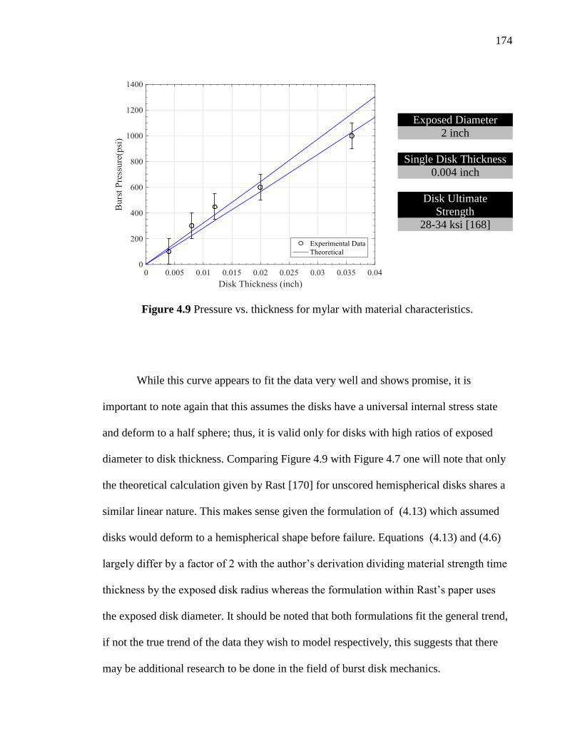
174
Exposed Diameter
2 inch
Single Disk Thickness
0.004 inch
Disk Ultimate
Strength
28-34 ksi [168]
Figure 4.9 Pressure vs. thickness for mylar with material characteristics.
While this curve appears to fit the data very well and shows promise, it is
important to note again that this assumes the disks have a universal internal stress state
and deform to a half sphere; thus, it is valid only for disks with high ratios of exposed
diameter to disk thickness. Comparing Figure 4.9 with Figure 4.7 one will note that only
the theoretical calculation given by Rast [170] for unscored hemispherical disks shares a
similar linear nature. This makes sense given the formulation of (4.13) which assumed
disks would deform to a hemispherical shape before failure. Equations (4.13) and (4.6)
largely differ by a factor of 2 with the author’s derivation dividing material strength time
thickness by the exposed disk radius whereas the formulation within Rast’s paper uses
the exposed disk diameter. It should be noted that both formulations fit the general trend,
if not the true trend of the data they wish to model respectively, this suggests that there
may be additional research to be done in the field of burst disk mechanics.

175
Upon closer review of literature, a formula, of similar nature to the author’s has
been derived by Peter Barlow [170] relating a cylindrical pipes (rather than a disk’s)
materials ultimate strength 𝜎𝑡, thickness t, and outer diameter do to burst pressure
Pburst(cyl):
𝑃𝑏𝑢𝑟𝑠𝑡(𝑐𝑦𝑙) =2 𝜎𝑢𝑙𝑡 𝑡
𝑑𝑜 (4.14)
In fact, as long as the radius of the disk is much greater (x50) than the thickness
the t2 term in Equation (4.13) is negligible and reduces to Equation (4.14).
4.3 Taylor Testing
An unintended but beneficial consequence of testing utilizing a polycarbonate
sabot during a normal impact between a steel flyer and large plate was a sabot with a
shorted length and an enlarged cross-section. This redistribution of sabot mass was a
result of both plastic and inelastic deformation occurring upon impact. The resultant
sabot shape was reminiscent of similar tests carried out by G.I. Taylor [171], which
related dynamic yield stress of materials to the velocity of impact for cylinders where the
ratio of end length to initial lengths are greater than 0.5. Reviewing his paper we find the
impact velocity V is expressed in the following formula:

176
𝑉 = ((𝐿𝑖−𝑋
2(𝐿𝑖−𝐿𝑓)
1
ln (𝐿𝑖/𝑋))
𝜌𝑝
𝜎𝑦)
−1
2
(4.15)
where 𝜎𝑦 is yield stress, 𝜌𝑝 is density, V is the impact velocity, Li is the initial
length, LF is the final length, and X is the length of the undeformed section.
This formula was then applied to the sabot shown in Figure 4.10 below.
Figure 4.10 Post shot sabot profile, for a projectile shot at 600 psig.
In the derivation of Taylor’s formula, cylinders are of uniform diameter over
the length. The Marquette cylindrical sabot, however, has a tiered hollow pocket
(see Figure 2.10), which modify the initial assumptions of Taylor’s equation.

177
In order to address this, the dimensions of the sabot have been taken
removing the lengths added by the lips. The initial length is easily found by
referencing the dimensions of the drafted sabot in Figure 2.10 and the final length
can also be measured by discounting the length added by the lighter shades of
polycarbonate captured in Figure 4.10.
Utilizing this above formula (4.15), one finds the sabot’s impact velocity within Table
4.2.
Table 4.2 Reverse Taylor Test for Impact Velocity
Variable Magnitude Variable Magnitude
𝜎𝑦 9000 psi Li 3.875 inch
𝜌𝑝 0.044 lb./inch3 Lf 3.379 inch
V 268 ft./s X 2 inch
The calculated velocity of 268 ft./s underestimates data taken from the
piezoelectric pins (280 ft./s) by approximately 5%, with error stemming from a non-
uniform sabot cross-section and interference from features such as the aforementioned
sabot lips and original mounted flyer (not shown). While the Taylor equation gave a good
estimate for velocity in this test, at higher pressures, it is thought that the Taylor test will
lose accuracy. This due to the clear plastic deformation, and fracture noticed, in other
sabots, like the one shown in Figure 4.11 below:

178
Figure 4.11 Post shot sabot profile; sabot shot at 960 psig.
4.4 Catch Tank Pull Down
In the muzzle velocity calculations, it was assumed that there was no forward
pressure on the sabot. To achieve this, the entire section forward of the sabot, comprising
a ~2.5m3 volume, was pulled down to pressures below ~200 mTorr for flyer plate studies.
For future pressure shear studies, a recommended pressure of ~50 mTorr was suggested
by Bill Reinhardt of the Aeroballistics Range Association. This was later noted to be the
pull down pressure utilized by the Georgia Tech Shock Physics team, upon visit to their
facility.
These low pressures are maintained not only to prevent forward pressure on the
sabot during flight, but also to prevent pillows of air from accumulating in front of the

179
flyer on its trajectory down the barrel, which can interfere with both experiment
orientation as well as data collection.
To reach these pressures, an Agilent DS602 pump was utilized in conjunction
with Marquette University’s shop vacuum system. While the building vacuum system
was able to both pull a vacuum quickly and later provide a path for post shot particulate
removal, the shop vacuum bottomed out at ~21 in Hg (533400 mTorr), well above both
target pressures. The Agilent pump, known in the industries as a “scroll” roughing pump,
works well between atmospheric pressure in the region of viscous flow.
In order to determine the region in which the pump operated, the Knudsen
number, a non-dimensional number charactering the mean free path of a particle and a
relevant length, D, often the diameter through which a flow is piped [173], was used.
Kn =λ
𝐷 (4.16)
For spherical particles, the mean free path 𝜆 can be expressed:
𝜆 =𝑘 𝑇
√2 𝜋 𝑑3 𝑃 (4.17)
where P is pressure, T is temperature, d is the molecular diameter, and k is the
Boltzmann’s constant. Typical temperature within the lab is 295 K, the piping diameter is
3.5 cm and the gas filling both the vacuum and target tanks is air (primarily nitrogen).

180
Looking at the CRC handbook [174] one finds the Boltzmann’s constant,
1.38064852×10⁻²³ m2kgs-2K-1 and the mean molecular diameter of a diatomic nitrogen
molecule, 364 picometers.
Before using these equations, a brief explanation of the three flow regimes, shown
in Figure 4.12, may be helpful. As a vacuum pump begins to evacuate a chamber, flow
initially is of a viscous nature, molecules have a relatively short mean free path, and
collisions between molecules are frequent. This means that initially particles will often
“flow” in the same direction as voids created by the moving of particles, Group A, in a
single direction will allow other particles behind the original moving front, Group B, to
fill the void space. A third group of particles, Group C, will also push Group B forward
as they collide between Group C and the group behind them, Group D, et cetera. In short,
there is a high potential pressure between high and low pressure areas. As flow begins to
transition to Knudsen flow, more and more space is free of particles and groups of
particles become increasing sparse. Particle groups quickly intermingle, increasingly less
likely to travel in the desired direction, as areas and the difference between the high and
low pressure sources becomes much lower, decreasing flow rate. Finally, as flow
transitions to the molecular range, particles have higher likelihood to collide with the
walls of the container holding them rather than colliding with another particle. This
means that decreasing pressure becomes more a question of a particle bouncing out of the
system and unable to return than a flow that can be influenced.
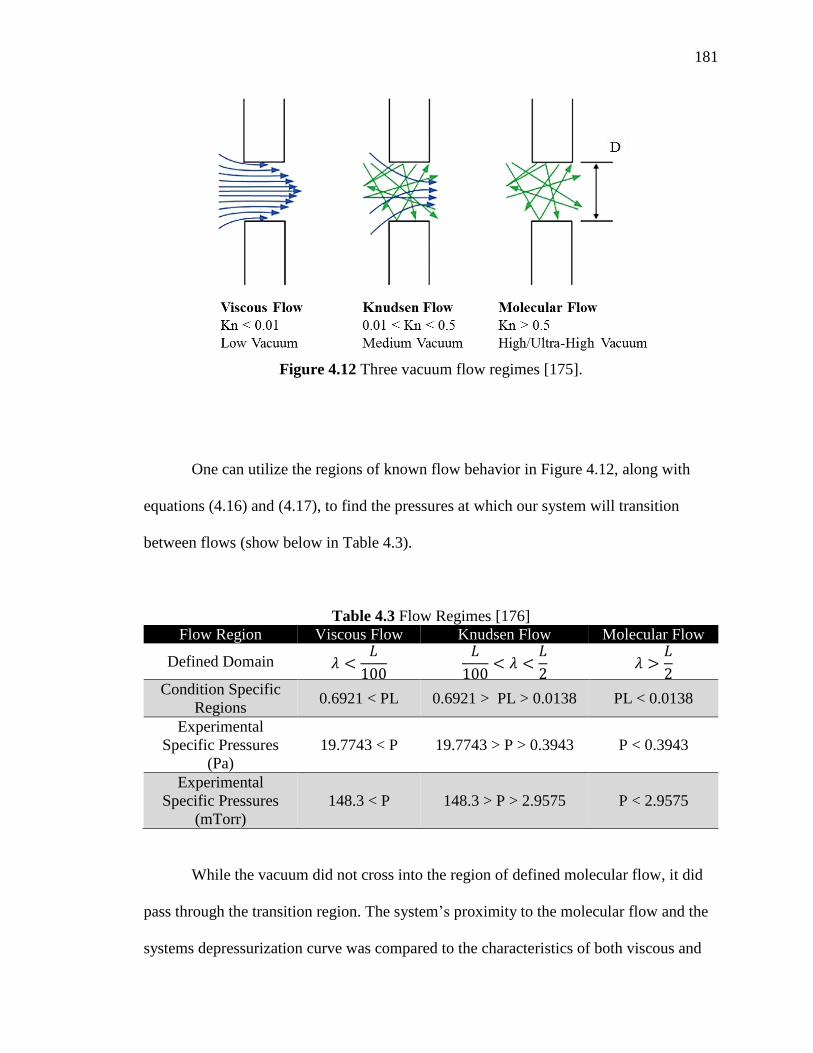
181
Figure 4.12 Three vacuum flow regimes [175].
One can utilize the regions of known flow behavior in Figure 4.12, along with
equations (4.16) and (4.17), to find the pressures at which our system will transition
between flows (show below in Table 4.3).
Table 4.3 Flow Regimes [176]
Flow Region Viscous Flow Knudsen Flow Molecular Flow
Defined Domain 𝜆 <𝐿
100
𝐿
100< 𝜆 <
𝐿
2 𝜆 >
𝐿
2
Condition Specific
Regions 0.6921 < PL 0.6921 > PL > 0.0138 PL < 0.0138
Experimental
Specific Pressures
(Pa)
19.7743 < P 19.7743 > P > 0.3943 P < 0.3943
Experimental
Specific Pressures
(mTorr)
148.3 < P 148.3 > P > 2.9575 P < 2.9575
While the vacuum did not cross into the region of defined molecular flow, it did
pass through the transition region. The system’s proximity to the molecular flow and the
systems depressurization curve was compared to the characteristics of both viscous and

182
molecular flow. According to Y. Senda [177], one can calculate the pump-down time by
examination of flow at both conditions. As mentioned within his paper, the flow rate of a
gas evacuated from a system is normally calculated by a flow rate equation shown below:
𝑄 = 𝐶 (𝑃1 − 𝑃0) (4.18)
where Q is the flow rate, C is conductance, P0 is the low pressure side and P1 is the high
pressure side. The conductance for the system varies based on the flow condition and
formulas are included below in Table 4.4.
Table 4.4 Conductance Values for Long Pipes [178]
Viscous Flow Molecular Flow
Conductance 1349 𝐷4 𝑃
𝐿
121 𝐷3
𝐿
D in the above table is smallest hose diameter in the vacuum pumping line, P is the current pressure and L
is the length of the hose line
To solve the problem of a transition region Y. Senda employs the use of a transferring
pressure which marks a transition between the regions of viscous and molecular flow
[177].
𝜋 =𝑆𝑜
𝐶𝑐 (4.19)

183
where 𝜋 is the transference pressure, So is the pumping speed and Cc is the conductance
coefficient for viscous flow (found in Table 4.4). From this, one can switch between two
equations:
one for viscous flow:
𝑃 ≈ 𝑃𝑜 𝑒𝑥𝑝(−𝑡 𝑆𝑜
𝑉) (4.20)
and one for molecular flow:
𝑃 ≈2 𝜋 𝑉
𝑡 𝑆𝑜 (4.21)
where P is the final pressure, Po is the initial system pressure, t is the elapsed time, So is
the pump speed, and V is the system volume.
In order to test our system, which did not have a constant pumping speed, the
pumping curve from the Agilent DS602 vacuum pump was fit with a piecewise 3rd order
polynomial curve as shown in Figure 4.13 below.

184
Figure 4.13 Manufacturer pump curve with fitting [179].
Based on literature from the manufacturer the black curved lines were generated by
placing a vacuum gauge on the top of the vacuum pump inlet and turning the pump on.
The lab’s Agilent DS602 pump curve is the upper most black line with other models
curves below.
This curve was employed, along with initial conditions, to solve for the estimated
time required to evacuate the chamber show in Figure 4.14 below. As can be seen, the
high pressure data taken from the vacuum gauge falls along the viscous flow curve.
Between the high pressure and low pressure data, there is a region where measurements
cannot be taken as the gauges do not overlap in measuring range. Around the start of the
low pressure data, taken with the digital KJL vacuum gauge, flow begins to transition
between molecular and viscous flow (Knudsen Flow). Before gas flow is reached
characteristics of a fully molecular flow, leaks and outgassing within the system begin to
take effect and reduce the speed at which the vacuum is pulled. This is until the system

185
reaches a state of equilibrium between the gases entering and the gases pulled from the
system.
Figure 4.14 Pressure and pumping speed within the system as a function of time.
As can be seen from Figure 4.14, the numerical fit matches well with experimental
data. Missing data between high and low pressure regions results from vacuum gauges
with operational regions that do not overlap (see section 2.2.7). System leaks noted here
were determined by first reaching a low pressure and monitoring the increase of pressure

186
over a period of 10 minutes. The lowest leak rate identified was around 1 millitorr per 30
seconds, though a more typical rate is around 0.5 millitorr per second, which is the rate
utilized in the figure above. This leak rate stems from both traditional leaks, as well as the
outgassing of various materials such as the rubber on the impact plate within the catch
tank. This outgassing phenomenon was especially noticeable when, in an effort to find a
method of slowing the sabot, a plethora of old lab cotton coats were added to the breach.
While the coats did a good job of slowing the projectile and lessening the impact against
the impact plate within the catch tank it also dramatically increased the amount of time to
pull down the system to well over 3 hours.
4.5 Muzzle Velocity
This section presents the derivation of the most common methods of estimating
maximum muzzle velocity and the travel time of the sabot down the barrel.
ISOBARIC
While the experimental behavior of the gun remains in progress, a need to
anticipate projectile velocity accurately was required. In order to anticipate behavior,
various models were tested and compared to ensure the best possible fit. Before
researching additional methods of determining projectile velocity, a series of ideal gas
relations were used, which assume that gas properties remain uniform both behind the
sabot and throughout the breach chamber.

187
Isobaric, the simplest of models, assumed that the pressure behind the projectile
was constant meaning that since the area aft of the projectile was also constant an
acceleration and velocity could be easily determined.
The force F, moving the projectile, is simply the pressure P acting on the sabot’s
aft area A:
Fsurface = Pprojectile surface A (4.22)
The force balance is simply the mass m, and acceleration a of the particle
influenced by the frictional force f, and pressure force.
Fsurface − f = ma (4.23)
As the pressure behind the projectile P is constant, a constant force is applied
meaning that the acceleration is also constant.
Pprojectile surface = Constant = Pi (4.24)
Pi A−f
m= a

188
(4.25)
One can integrate backwards, to solve for both velocity v, and position x, with
respect to time t:
v(t) = at + vo where vo = 0 and v(0) = 0 (4.26)
x(t) =a
2t2 + v0t + xo where xo = 0 and x(0) = 0 (4.27)
Since the known position at the final time is the barrel length L, one can find the
final time tf through the use of equations (4.25) and (4.27):
x(tf) = L =Pi A−f
2 mtf
2 + 0 + 0 (4.28)
√2 m L
Pi A−f= tf (4.29)
As the equation for final velocity is also known one can substitute the final time
from equation (4.29) to find the isobaric velocity in equation (4.26):
v =Pi A−f
m tf (4.30)
v =Pi A−f
m√
2 m L
Pi A−f= √
2 m L (Pi A−f)2
(Pi A−f) m2 (4.31)
v = √2 L (Pi A−f)
m (4.32)

189
This equation, however, was anticipated to be inaccurate, as the initial amount of
gas stored within the starting volume would have to expand to fill the increasing volume
behind the projectile, as it traveled along the barrel. An isothermal equation allowed for
the pressure behind the projectile to vary, as the chamber increased in volume.
ISOTHERMAL
Beginning with the work-energy method, the kinetic energy of the sabot
composed of the sabot’s the mass m, and velocity v, is balanced with the frictional force
f, exerted over the barrels length L, and pressure P, acting on the sabot for from the initial
Vi to final Vf volume:
KE = ∫ P dVVf
Vi− f L = 1
2 ⁄ m v2 (4.33)
The frictional force f, used here can either be assumed to be a constant characterized by
the coefficient of friction between the lubricated rubber orings and steel barrel and the
normal force of contact between the orings and the barrel or a function of velocity.
Typical hand mounting of the sabot into the breach is easy and requires little force. The
friction opposing motion is negligible with respect to the high pressures driving the sabot
during an experiment so while equations are formulated with friction this is omitted in
calculations.

190
The current pressure can be found by the ideal gas law through the use of volume
V, number of moles n, universal gas constant R, and temperature T:
P =n R T
V (4.34)
A substitution of equation (4.33) into equation (4.34) and factoring out the
constants allows for the integration of work done on the projectile by the compressed gas:
KE = ∫ n R T
V dV
Vf
Vi− fL (4.35)
KE = nRT∫dV
V
Vf
Vi− fL (4.36)
KE = nRT ln (Vf
Vi) − fL (4.37)
Since the initial pressure Pi and initial velocity Vi are equal to the constants
removed:
PiVi = nRT (4.38)
the substitution of equation (4.38) into equation (4.37) yields,

191
12⁄ mv2 = PiViln (
Vf
Vi) − fL (4.39)
The final volume is equivalent to the initial volume, plus the surface area of the
bore A, multiplied by the length of the barrel L:
Vf = Vi + AL (4.40)
So, substituting equation (4.40) into (4.39) and solving for v, one finds the
isothermal sabot velocity equation:
v = √2PiViln(
Vi+AL
Vi)
m−
2fL
m (4.41)
ADIABATIC
The isothermal formulation did not account for the molecules of gas to change
temperature. According to the Joule-Thompson effect as the gas chamber emptied, much
in the same way a spray can or air can empties, the gas would decrease in temperature,
removing some energy in the form of pressure. Therefore, a reversible adiabatic
condition, implying isentropic gas expansion was assumed. As the volume expansion of

192
the gases are quite fast, the system will certainly generate entropy (leading to
overestimates in sabot velocity), however the adiabatic assumption is certainly better than
the isobaric or isothermal assumptions. Again, a work-energy method was used with the
sabot’s mass m and velocity v, balanced against the frictional force f exerted over the
barrels length L and pressure P acting on the sabot from the initial Vi to final Vf volume:
∫ PdVvf
vi− fL = 1
2⁄ mv2 (4.42)
This time, the polytrophic relationship (with an exponent of γ, for an adiabatic
process) [180] relating pressure to volume V and the ratio of specific heats γ was used to
separate pressure into its variable and constant components:
ln(PVγ) = Constant = PVγ (4.43)
P =C
Vγ (4.44)
Substituting equation (4.42) into equation (4.44), one can remove the constant and
integrate with respect to volume:
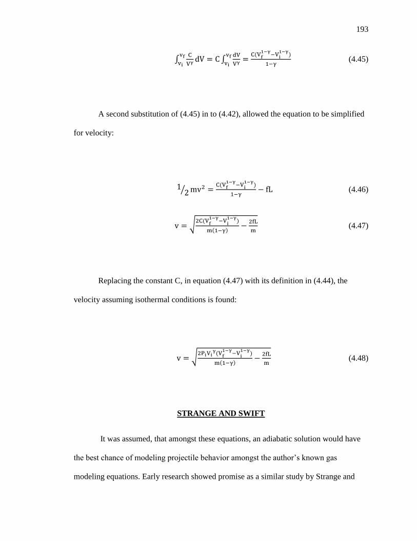
193
∫C
Vγ dVvf
vi= C∫
dV
Vγ
vf
vi=
C(Vf1−γ
−Vi1−γ
)
1−γ (4.45)
A second substitution of (4.45) in to (4.42), allowed the equation to be simplified
for velocity:
12⁄ mv2 =
C(Vf1−γ
−Vi1−γ
)
1−γ− fL (4.46)
v = √2C(V
f1−γ
−Vi1−γ
)
m(1−γ)−
2fL
m (4.47)
Replacing the constant C, in equation (4.47) with its definition in (4.44), the
velocity assuming isothermal conditions is found:
v = √2PiVi
γ(Vf1−γ
−Vi1−γ
)
m(1−γ)−
2fL
m (4.48)
STRANGE AND SWIFT
It was assumed, that amongst these equations, an adiabatic solution would have
the best chance of modeling projectile behavior amongst the author’s known gas
modeling equations. Early research showed promise as a similar study by Strange and

194
Swift [181] also utilized an adiabatic equation to model gas behavior with an able
equation of state. In the equation below, variables include initial pressure Po, initial
volume Vo, the specific heat ratio K, the area on the rear of the sabot A, mass m, moles of
ideal gas n, gas co-volume per mole b, and the sabot velocity v:
v =√
2Po(Vo−nb)(1−(Vo−nb
Vo−nb+Ax)K−1
)
m(K−1) (4.49)
It should be noted that both the nitrogen and helium behave as ideal gases and so
alternate equations of state such as Able and Van der Waals have only small effects on
the velocity profiles of the gas gun. Both helium and nitrogen are modeled as ideal gases
up to the pressures utilized in this experimental setup with compressibility factors close
to 1, as shown in Figure 4.15. It should be kept in mind that high pressures are only seen
at the very onset of breach depressurization and quickly fall back to ideal behavior. To
properly include more complex equations of state would increase computational time as
state would have to be found for each time step.

195
Figure 4.15: Compressibility factors of nitrogen and helium [182].
LAGRANGE
Until this point, it has been assumed that the gas within the system behaves in a
uniform fashion. However, state properties are non-uniform as the gas gun fires. In doing
so, the true energy of the gas has been neglected and, this requires correction with an
extended deviation, which mirrors that of one done by Ballistics Theory and Design
[150]. This equation approximates the gradient of information within the barrel and
breach as Lagrangian, utilizing Lagrange’s own method [183]. The equations within the
text assume that the breach pressure is created utilizing an explosive charge (i.e.
supersonic shock/pressure wave). In practice, this gives generally higher initial
acceleration, as the expanding gas creates a favorable pressure gradient at the onset and
through the initial flight of the projectile before decaying. This is opposed to a

196
compressed gas shot, which starts with a uniform pressure state and decays immediately
to an unfavorable gradient with pressure waves interacting and creating an expanding
series of problems.
Figure 4.16 An x-t diagram of pressure waves emanating from the voids left by the sabot
[150].
The derivation below has been completed following the aforementioned
derivation assuming no explosives charge. Assuming a 1D behavior is an acceptable
assumption, though the diameter differences between the breach and barrel make it an
imperfect one. Later calculations will assume that the breach is of the same diameter as
the barrel while the amount of gas as compared with the experimental setup remains
constant. As in profiles derived before, it is assumed that the gas density profile is a
function of time and is uniform in space. While this assumption might be valid for slow
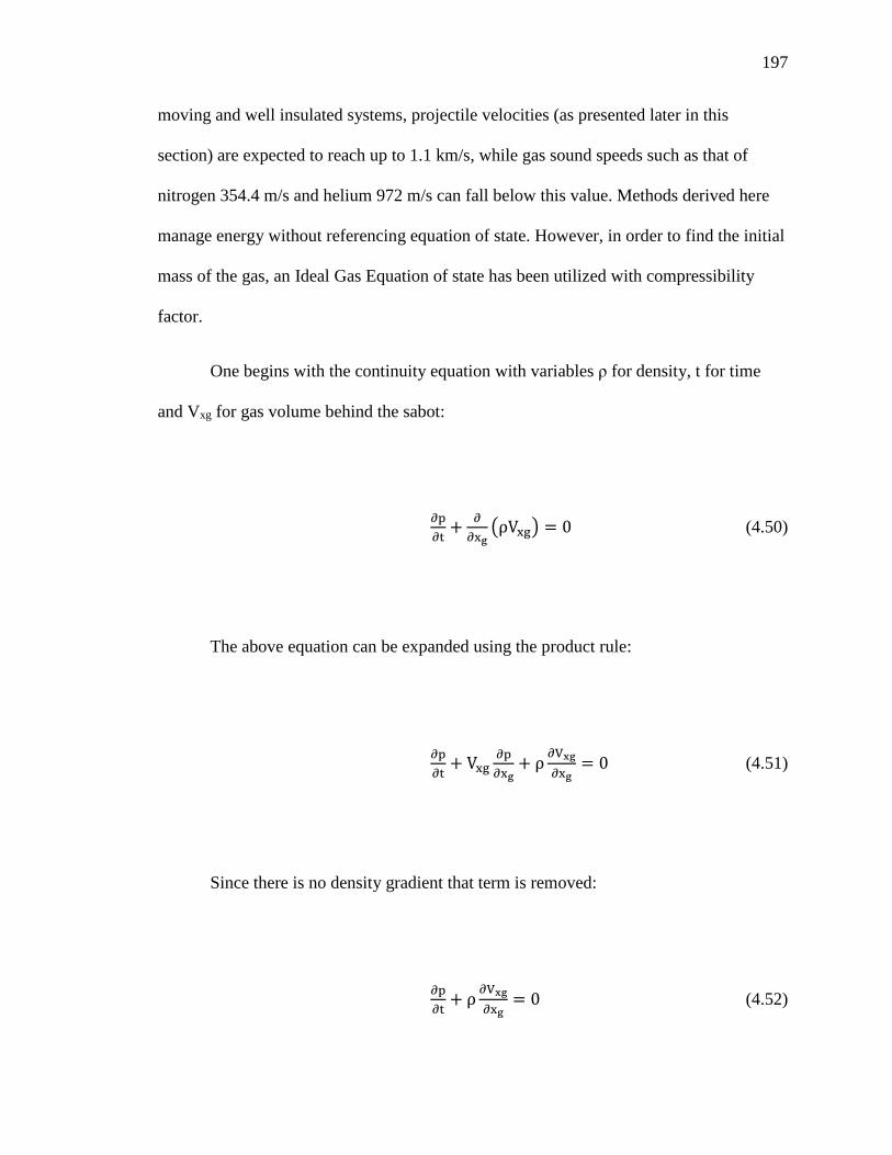
197
moving and well insulated systems, projectile velocities (as presented later in this
section) are expected to reach up to 1.1 km/s, while gas sound speeds such as that of
nitrogen 354.4 m/s and helium 972 m/s can fall below this value. Methods derived here
manage energy without referencing equation of state. However, in order to find the initial
mass of the gas, an Ideal Gas Equation of state has been utilized with compressibility
factor.
One begins with the continuity equation with variables ρ for density, t for time
and Vxg for gas volume behind the sabot:
∂p
∂t+
∂
∂xg(ρVxg) = 0 (4.50)
The above equation can be expanded using the product rule:
∂p
∂t+ Vxg
∂p
∂xg+ ρ
∂Vxg
∂xg= 0 (4.51)
Since there is no density gradient that term is removed:
∂p
∂t+ ρ
∂Vxg
∂xg= 0 (4.52)

198
1
ρ
∂p
∂t= −
∂Vxg
∂xg (4.53)
The density is simply the mass of the gas G, over the volume of the container V:
ρ(t) =G
V(t) (4.54)
The volume being a function of area A and barrel length L, can be inserted:
V(t) = AL(t) (4.55)
AL(t)ρ(t) = G (4.56)
Differentiating with respect to time:
1
L
dL
dt=
∂Vxg
∂xg (4.57)
Integrating with respect to xg, while utilizing the knowledge that xg = 0 when
Vxg = 0, one finds a relation with velocity v:

199
v
L=
Vxg
xg (4.58)
While this does not give a complete property gradient within the gas gun, it does
give a linear gas velocity gradient and allows for the derivation of the kinetic energy of
the gas:
KEg = ∫1
2mgVxg
2 dxgL
0=
1
6ρALv2 =
1
6Gv2 (4.59)
The book, Ballistics Theory and Design, continues with an adiabatic condition
utilizing the ratio of specific heats 𝛾, initial pressure Pi, final pressure Pf, initial volume
Vi, final volume Vf, and breach length LBr, assuming that the breach and bore are of the
same area A, underestimating the idealized profile:
Pf
Pi= (
Vf
Vi)−γ
= ((LBreach+L)A
(LBreach)A)−γ
(4.60)
With the adiabatic condition, the pressure work W, acting on the rear surface of
the projectile is expressed:
200
W = APi ∫ (LBreach+x
LBreach)−γdx
L
0 (4.61)
The resultant equation (4.61) was inserted into an energy balance, accounting for
the kinetic energy of the gas (4.59), and the resistance from friction and kinetic energy of
the sabot (4.42), where m is the sabot mass, and f is the force of friction:
1
6cv2 + 1
2⁄ mv2 + fL = APi(L+LBr)
1−γ−(LBr)1−γ
(1−γ)(LBr)−γ (4.62)
The initial pressure:
Pi =λG
ALBr
(4.63)
λ = RT (4.64)
(G
3+ m)v2 = 2A
λG
AL Br
(L+LBr)1−γ−(LBr)
1−γ
(1−γ)(LBr)−γ− 2fL (4.65)
v = √2AλG(LBr)1−γ
AL(1−γ)(LBr)−γ(m+G
3)[(LBr+L)1−γ
(LBr)1−γ − 1] −2fL
(m+G
3) (4.66)

201
Simplifying, one arrives at the Lagrangian definition for projectile velocity:
v = √2λG
(1−γ)(m+G
3)[(L𝐵𝑟+L)1−γ
(L𝐵𝑟)1−γ − 1] −2fL
(m+G
3) (4.67)
A new kinetic energy balance consists of this above gas energy along with the
projectile kinetic energy, drag, and adiabatic energy derived above. This equation does
not account for gun cambridge (the difference between the barrel diameter and breach
diameter) between the barrel and breach.
1
6Gv2 + 1
2⁄ mv2 + fL =G(Vf
1−γ−Vi
1−γ)
1−γ (4.68)
1
6Gv2 + 1
2⁄ mv2 =G(Vf
1−γ−Vi
1−γ)
1−γ− fL (4.69)
Gv2 + 3mv2 =6G(Vf
1−γ−Vi
1−γ)
1−γ− 6fL (4.70)
v2(G + 3m) =6G(Vf
1−γ−Vi
1−γ)
1−γ− 6fL (4.71)
v = √2PiVi
γ(Vf1−γ
−Vi1−γ
)
(1−γ)(G+3m)−
6fL
(G+3m) (4.72)

202
PIDDUCK AND KENT
Lagrange’s problem was later extended, as the forward moving projectile created
vacuum spaces behind itself as it traveled forward. Information of state takes time to
travel from the rear of the projectile to the back of the breach. From the Newton-Laplace
equation it can be seen that the sound speed of a gas is a function of density and pressure:
ao = √γ P
ρ (4.73)
where ao is the sound speed of the gas, γ the ratio of specific heats, P is the gas pressure,
and ρ is the gas density. However, if one assumes that these gases can be well
characterized by the kinetic theory of gases, one finds that:
P =1
3ρcrms
2 (4.74)
where crms is the root mean square of molecular sound speed. Substituting, it can be seen
that the sound speed of the gas can be characterized by the root mean squared of the gas
and the specific heat of the gas.

203
ao = √γ
3 crms
2 (4.75)
One can find the root mean squared speed of a molecule from the temperature and molar
mass of the gas:
crms = √3RT
M (4.76)
Where R is the ideal gas constant, T is temperature, and M is molar mass. Substituting
one final time, the common formulation for the sound speed of a gas is found:
ao = √γRT
M (4.77)
As can be seen, the sound speed of the gas varies from gas to gas with smaller
molecular compounds having a generally higher sound speed. In addition, raising gas
temperature also raises gas sound speed. Reviewing the literature, experimenters have
had great success in increasing gas gun performance through the use of smaller molecular
compounds. However Hallock Swift notes that while he and his team at NRL we able to
“demonstrate initial gas temperatures up to 3000 K... [with] sound speed increases up to a

204
factor of 2.5 above room temperature… expected. In every case, the light-gas gun could
be made to achieve launch velocities as great as those achieved when the gun was fired at
room temperature, but no performance increase could be achieved” [166].
Three gases are commonly utilized in gas gun as the driving gas. At standard
pressure and atmosphere, these include nitrogen, with a sound speed of 354.4 m/s, helium
at 972 m/s, and hydrogen at 1270 m/s. Nitrogen has the lowest of the three sound speeds,
but is readily available. Hydrogen is the fastest of the three, but gases has a tendency to
react with oxygen and is hazardous. Helium is the second fastest, but it is the most
expensive.
To understand the effects of sound speed on velocity, one can look to an equation
by Hernri Bernier [167], which utilizes the perfect gas equation, coupled with constant
specific heat:
P = Po [1 −γ−1
2∗aov]
2γ
γ−1 (4.78)
Where P is the final pressure, Po is the initial pressure, γ is gas specific heat, ao is
gas sounds speed, and v is velocity. Bernier mentions that for a complete release of gas,
that is to say the gas has the ability to expand behind the projectile infinitely, (p=0), one
can generate a theoretical peak projectile velocity given by the equation:

205
vlim =2ao
γ−1 (4.79)
Using this equation, Bernier proceeds to tabulate the relative effectiveness of each gas
(Table 4.5).
Table 4.5 Maximum Projectile Velocity of Various Gases
Gas Γ ao (m/s) vmax
Nitrogen 1.4 343 1715
Helium 1.663 970 2926
Hydrogen 1.406 1258 6197
As one can see gases of a lower molecular size tend to have a higher sound speed
and though the specific heat can negatively affect peak velocity, the sound speed is
generally hundreds of magnitudes higher in effect. The peak velocities shown in Table
4.5 do not take the projectile mass, breach to bore diameter, nor a reasonable length of
gun barrel into account.
It is for this major reason that by changing the gases, one can radically change the
gun’s peak velocity, a variable that the above equations fail to take into account. Notable
steps to the derivation of the Pidduck and Kent solution included work by Huguenot
[184], Love [43], Pidduck and Kent [42]. These all share a role in applying the pressure
wave theory caused by the expansion disturbances of the forward motion of the
projectile. The resultant equation is as follows, assuming that the breach and barrel are of
the same diameter. This solution accounts for non-uniform density and pressure:

206
v = ao√ao
γ−1
√1−(1+
γ(poA1L
mao2 )
G/m)
(1−γ)
γ−1 (4.80)
Where ao is related to G/m by:
G
m=
2γ
γ−1ao(1 − ao)
−γ
γ−1 ∫ (1 − a0μ2)dμ
1
0 (4.81)
which can be expanded by a mixed power binomial series or solved numerically.
This equation can also be corrected to account for differences in barrel and breach
diameter by adjusting the sound speed and driving pressure:
pc = po (1 + [(γ+1
2)1/2
− 1] (1 −A1
Ao))
2γ
(γ−1)
(4.82)
ac = ao [1 + [(γ+1
2)1/2
− 1] (1 −A1
Ao)] (4.83)

207
Additional information on the derivation and formulation of the Pidduck and Kent model,
which the author found useful, were found in the following sources: [186][187][188] and
further numerical formulations can be found in [189][190][191][192].
From Siegel, one could divide the operational parameter space of a gas gun into
three non-dimensional constants, which can and have been used to explore gas gun
performance space [44], shown in the three equations below and which can be seen
within the above equations:
m = p =G
m (4.84)
x =PAcL
mas2 (4.85)
u =u
as (4.86)
where m, x, and u are dimensionless mass (or pressure), length, and velocity respectively.
G is the mass of the gas within the breach, m is the mass of the projectile, P is the breach
pressure, Ac, is the barrel cross-sectional area, L is the position of the projectile along the
barrel, as is the sound speed of the driving gas, and u is the velocity of the projectile.

208
Table 4.6 Summary of Pressure Velocity Relations
Model Equation(s)
Isobaric v = √2L (PiA−f)
m (4.32)
Isothermal v = √2PiViln(
Vi+AL
Vi)
m−
2fL
m (4.41)
Adiabatic v = √2PiVi
γ(Vf1−γ
−Vi1−γ
)
m(1−γ)−
2fL
m (4.48)
Lagrange v = √2λG
(1−γ)(m+c
3)[(L𝐵𝑟+L)1−γ
(L𝐵𝑟)1−γ − 1] −2fL
(m+G
3) (4.72)
Pidduck and Kent
v = ao√ao
γ−1
√1−(1+
γ(poA1𝐿
mao2 )
G/m)
(1−γ)
γ−1 (4.80)
Utilizing the above models, the velocity profiles for pure nitrogen and a 0.25kg
sabot, traveling without friction effects are plotted in Figure 4.19 below. Initial testing
utilized building air, which is mostly comprised of nitrogen, and friction effects are also
considered negligible, but are not zero, so it is assumed that velocities shown here are
slightly above expected experimental observations. Other gases such as hydrogen or
helium (included in Figure 4.17 below), having higher sound speeds, increase peak
velocity attained by the projectile as expected from equation (4.79). Experimental data,
taken from: velocity blocks, dynasen pins, PDV, and reverse Taylor testing, within the
Figure 4.17, seem to have good agreement with initial analytical estimate of peak
projectile velocity.

209
Figure 4.17 Approximate gas gun pressure velocity profile for a variety of models for a
0.25 kg projectile.
From this, it can be seen that for a typical experiment one might expect peak
velocities around 720 m/s with nitrogen and 1120 m/s with helium. Only a single
experiment for a 0.25 kg sabot has been conducted thus far and the slight
underperformance is likely due to frictional forces between the sabot and the barrel. To
reduce this effect, vacuum grease should be used to coat the sabot prior to loading into
the barrel. Silicone greases such as the Dow Corning high vacuum grease are shear
thinning meaning that its viscosity decreases under shear stain. This also helps reduce
frictional effects. Experiments conducted up to 600 psig, (the peak pressurization tested),
and at other pressure and mass configurations have since shown good agreement with the
non-dimensionalized breach corrected Pidduck and Kent equation shown in Figure 4.18.

210
Figure 4.18 Non-dimensionalized pressure velocity curves with three observed tests.
The above graph is useful as it allows for the evaluation of pressure velocity
relations for multiple projectile masses rather than a single mass as presented in Figure
4.17. Unfortunately, while non-dimensionalization works well over a range of pressures
and projectile masses, it does not account for differences in the properties of the driving
gas. Helium, while known to achieve higher velocities than nitrogen, has a much higher
sound speed and lower molecular weight than Nitrogen and thus appears below the
Nitrogen curve in Figure 4.18.
From the Pidduck and Kent solution, instantaneous velocity is calculated as a
function of length along the barrel. From this estimation in velocity, one can also back
211
out the total time required for the sabot to travel the length of the barrel using the
following equation:
t = ∫1
vp(x)dx
L
0 (4.87)
where the time t for the projectile to fly the length of the barrel L is the length of the
barrel, and vp(x) is the velocity of the projectile at point x along the barrel. Using
calculated data, one can estimate time using the trapezoidal method as shown in Figure
4.17 below. Please note here that the number of trapezoids shown here are low so as to
demonstrate the principle, for better estimates of time one should decrease the distance
between each trapezoidal sample. The trapezoidal rule used in this calculation is included
alongside Simpson’s rule in Appendix B for increasing accuracy with larger distances
between samples and shorter calculation times.

212
Figure 4.19 Estimation of sabot travel time (converged to 7.87 millisec) for a 0.25 kg
projectile with a breach pressure of 10,000 psig.
4.6 Post Shot Pressure
By pulling a vacuum on the system a sub-atmospheric post shot pressure was
expected for most shots. This section quantifies the range of post shot pressures expected
for various breach pressures. To calculate the pressures, either the expected post shot
pressure free or Joule expansion [185] was assumed. One can assume free expansion, as
conduction of through the walls of the system, was known to operate at a much longer
time scale than the shot itself. As with the above equations, one could assume that the gas
within the chamber can be modeled as an ideal gas under adiabatic conditions, assuming
that the internal energy of the system does not change, that is to say that the effects of
213
heat transfer and work done on the system are negligible. The resultant equation , for
isentropic expansion, relates the pressure and volume of initial and final gas states:
Pf = Pi (Vi
Vf)γ
(4.88)
where Pf is the final pressure, Pi is the initial pressure, Vi is the initial volume, Vf
is the final volume, and γ is the gas specific heat. This equation, unlike the previous
section, simply jumps between states rather than iterating between time steps and
assumes no change in internal energy.
Utilizing the Engineering Equation Solver Package (EES), free expansion was
solved using state tables making use of known gas properties, initial pressure, initial
volume of the breach and the finial volume of the system to solve for free expansion.
Initial breach pressures are given in psig and final system pressures are given in in Hg to
ease comparison with existing dial gauge instrumentation within the shock physics lab
(Figure 4.20).
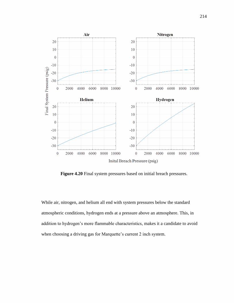
214
Figure 4.20 Final system pressures based on initial breach pressures.
While air, nitrogen, and helium all end with system pressures below the standard
atmospheric conditions, hydrogen ends at a pressure above an atmosphere. This, in
addition to hydrogen’s more flammable characteristics, makes it a candidate to avoid
when choosing a driving gas for Marquette’s current 2 inch system.

215
4.7 Gun Recoil
When designing the static gun components back in section 2.1, the peak recoil
force of the gun was required in order to find the preloading required by the various
threaded components.
From the definition of force [145], or using a momentum balance one finds that:
F =∆M
∆t (4.89)
Force F can be expressed as the relation between the change in momentum M over the
change in time t. From D.E. Carlucci and S. S. Johnson [150], one finds that the total
momentum of a gas gun can be expressed as:
∆M = (m +G
2) vMuzzle (4.90)
where M is the total momentum, 𝑚 is the mass of the projectile, G is the mass of the
propellant and vMuzzle is the muzzle velocity. From the previous section 4.5, all of these
variables are known, so the calculation of gun recoil force can be calculated for peak
operational pressure for both nitrogen and helium in Table 4.7.

216
Table 4.7 Gun Recoil Force
Variable Nitrogen Helium Units
Breach Pressure 68.95 (10,000) 68.95 (10,000) bar (psig)
Projectile Mass 0.25 0.25 Kg
Gas Mass 1.094 0.38 Kg
Travel Time 0.00787 0.00546 Sec
Projectile Velocity 718.33 1106 m/s
Total Momentum 572.51 486.64 kg m/s
Recoil Force 72.75 89.13 kN
5. CONCLUSIONS
5.1 Future Work
5.1.1 Gas Gun Improvements
While the work presented within this report has effectively designed a working
gas gun, which has been tested and utilized successfully in experimental testing, there
will always be ways to improve the system. Having reviewed the overall design through
the writing of this report, there are a few design modifications which should take
precedence.
5.1.2 Reinforcement of the Impact Plate and Target Tank
The first modification would be the bolstering of the impact plate. As mentioned
in section 2.1.5, the current steel chain used to restrain the impact plate is under spec for
breech pressures exceeding 1500 psig. While the chain should never be imparted with the
full force of gun recoil, a simple increase in chain diameter to one capable of

217
withstanding a dead load of 5,000 lbf. is inexpensive and easy to implement.
Additionally, it is proposed that a second steel plate be surmounted within the man-way
cover on the rear of the catch tank. Addition of this plate would not decrease performance
and would provide a second layer of defense within the catch tank. Finally, it was noted
that projectiles tended to fall to the floor of the catch tank after impact with the impact
plate. While this has not yet damaged the floor of the catch tank a rubber mat might
provide an additional cushion to pad the tank interior, reducing the chance of damage to
the tank interior.
5.1.3 Target Alignment
Through the build cycle much time was spent ensuring maximum work space
within the target tank, as space was at a premium. While experiments have successfully
taken place alignment of the flyer samples with the targets have been accomplished by
feel and line of sight. To this end a number of alignment techniques were discussed but
are yet to be fully implemented:
The Touch Method
The simplest of the three proposed alignment techniques the “Touch Method”,
aligns the projectile to the sample. In restoration of the Parthenon this method was used
to mate a blank piece of marble against an older sample of original material for a precise
fit matching all contours (Figure 5.1). When sample and target do not match, the target is
adjusted. While this method is simple and easy to understand, it has several flaws. The
most difficult part of alignment in this method is the need to move the sabot down and

218
back the entire length of the barrel, as the sabot will not fit between the target and barrel.
Shortening the sabot means the sabot will experience free flight where the sabot’s motion
is unconstrained. Removing the target plate after aligning the sabot is also a poor option,
as this voids the alignment. After the final placement of the projectile and target, the true
alignment of the projectile with the target plate cannot be quantified until readings from
break pins are collected post experiment.
Figure 5.1 Mating of two marble blocks [193].
The Harvard Method
For alignment of normal planar impact (as explained by Markos Hankin, Lab
Manager), Harvard utilizes a laser, optical flat and beam splitter to align the barrel sabot
and target to the same point (Figure 5.2). The laser is first aligned to the barrel by use of
an optical flat inserted facing the laser, first in the aft section of the barrel then in the
muzzle. Laser alignment is determined when the laser reflects back to the point of origin

219
from both locations. After the laser has been aligned to the barrel, the beam splitter is
affixed to the muzzle and the target is affixed with an optical flat. Since the beam splitter
is aligned with the length of the barrel, the first beam sent to the splitter should be
reflected back to the laser source. This is useful, as it provides one method of verifying
barrel alignment. The second portion of the laser beam is allowed through the splitter and
is reflected back from the optical flat affixed to the target. This system makes an
excellent alignment tool, as the laser light traveling the length of the barrel provides a
method of alignment that can be tuned by eye and by hand to within milli to micro radian
accuracy or higher (depending on the length the laser light travels).
Figure 5.2 Diagram of the Harvard optical alignment method.
This system was considered for use in alignment of Marquette’s samples but was
eventually discarded due to a need to machine specialty optical flats for the various
angles needed in pressure shear.

220
The Brown Method
Another method of target alignment published by Brown University [194]
(shown in Figure 5.3), utilizes an auto-collimating telescope along with a 90o prism with
mirrored surfaces on specific surfaces. Like the Harvard method, it uses laser light
emitted and bounced off mirrored surfaces on the muzzle and target surface. Unlike the
Harvard method, the brown method captures light between the target and flyer. Given the
shorter distance that the light travels, measurements need to be more precise. Older
autocollimators allow for this fine measurement of reflected light by eye for alignment
error of 2*10-5 radian, though many modern systems have dropped this functionality for
digital readouts (which often display a single peak received signal), which may hinder the
alignment of multiple signals on one collimator.
Figure 5.3 Optical alignment by use of the auto-collimating telescope [194].

221
A brief design, bouncing the light from an external auto collimator to the 90
degree prism using up to two penta-prisms, was initially considered as shown in Figure
5.4. While the Brown method promised the ability to align oblique pressure shear, flyer
plate alignment and the lack of space between the target and muzzle made placing and
aligning of equipment such as prisms, optical flats and the autocollimator itself both
tricky and time consuming.
Figure 5.4 Proposed method to employ the Brown method into the Marquette gas gun
design.
The Split Mirror Method
A final method proposed by the author is the use of an optical table placed
between the target and muzzle. Using a small rotatable table, mounting a laser beam
splitter and 2D optical receiver plate, it is thought that a significant range of oblique
angles could be aligned with relatively minimal difficulty during alignments.

222
Figure 5.5 A novel proposed method for the alignment of oblique impacts used in
pressure shear.
5.1.4 Examination of Surface Finishes for use with PDV
Within section 2.2.6, a brief examination of retroreflective surfaces for PDV was
discussed. These patterns, while manufactured at Marquette via laser cutting and
machining are recognizable (Figure 5.6) as the rectangular and triangular cuts desired, the
end results, while nominally accurate in shape are, at micrometer size, quite rough.
Figure 5.6 Samples cut by a metal cutting laser and triangular machining bit.

223
Since data arrives from the surface of samples shallower surface cuts and smaller,
accurate, features lower than the 50 – 200 µm (shown above) should provide better data.
To this end research into finer manufacturing techniques are underway with promising
work being performed at UW Madison (Figure 5.7) by Dr. Min and his Nano-Machining
Lab, which may be able to provide better surface definition for samples [195].
Figure 5.7 Demonstration of the ROBONANO α-0iB, creating a retroreflective surface.
5.1.5 Use of CTH and Shock Wave Theory for Experimental Design
Due to priorities and time constraints, this research was unable to conduct
extensive work within CTH ((𝐶ℎ𝑎𝑟𝑡𝐷2)3/2, ChartD squared to the Three Halves) with
simulations, such as like those shown below in Figure 5.8 or provide a complete section
within this work regarding wave propagation. After having read other works of past
graduate students within the Marquette University Shock Physics Lab Group, the author
is convinced that the enterprising reader will discover much information covering CTH,

224
KO, and Wave theory in a significant portion of past Marquette graduates work,
mentioned in section 1.2.3.
Figure 5.8 Flyer plate impact of aluminum impacting copper at 600m/s.
5.1.6 Experimental Testing
While some experimental testing is underway, initial testing has resolved a
number of minor details regarding optimal setup of PDV, laser gates and firing
procedure. It has only been within the most recent 2-3 shots that usable data has been
recorded and can be utilized for extensive research. Some of the future types of
experimental work are outlined in Figure 5.9 below.

225
Figure 5.9 Three common types of shock physics experiments.
Normal [196] and oblique impacts can be used to characterize wave speeds
through materials for use characterizing high stress material response, and shock sintering
allows for the development of new composite materials. Oblique impacts [197] allow for
the investigation of normal (longitudinal) as well as shear (transverse) waves (similar to
the two modes of vibration one might induce in a spring (Figure 5.10).
Figure 5.10 Transverse and longitudinal waves.

226
Shock sintering utilizes high pressure to shock bond granular materials together.
While traditional manufacturing techniques for composite materials often involve heating
materials for long time periods. This melts grain together, but comes at the cost of
annealing and loss of original grain structure. By shock sintering, the outer surfaces of
individual grains melt, welding grain to grain, then cool quickly maintaining grain
structure. A test shot for the shock sintering of a Sodium Dodecyl Sulfate with Sodium
Carbonate is shown below (Figure 5.11). Though materials in this shot did not likely
undergo sintering, the methods used in this shot provided researchers with a proof of
concept and confidence in the gas guns ability to perform such future experimental work.
Figure 5.11 1-9-2017 test shot for the shock consolidation of powders.

227
5.2 Closing
Figure 5.12 Completed 2 inch single stage dual diaphragm gas gun.
This concludes the master’s thesis, it is not by any means comprehensive, but it is
unlikely that it could ever be. After the construction of this system, it was intended to
provide a broad overview of the single stage gas gun setup and a brief introduction to the
major components on which the Marquette 2 inch single stage dual diaphragm gas gun
operates, this has been completed herein. It is my hope that some reader in the future
might use this as a foundation to produce an even more substantial work. To this reader
“take what you can and burn the rest”! If you need help or clarification, please contact
me, as it would be a pleasure to return the contact. Unfortunately, time spent within this
universe is finite, so there may eventually be complications with communications.

228
Questions then should be asked to a colleague or held until meeting with The Higher
Authority. The author’s family has a saying, amongst others, which the author has found
useful in research “man plans, God laughs.”
God Bless,
Nathaniel ϟteven Helminiak

229
6. WORKS CITED
[1] Ferrill, A., 1997. The origins of war: From the stone age to Alexander the Great.
Westview Press.
[2] Thieme, H., 2005. Die ältesten Speere der Welt-: Fundplätze der frühen Altsteinzeit
im Tagebau Schöningen. Archäologisches Nachrichtenblatt, 10(4), pp.409-417.
[3] Lahr, M.M., Rivera, F., Power, R.K., Mounier, A., Copsey, B., Crivellaro, F., Edung,
J.E., Fernandez, J.M., Kiarie, C., Lawrence, J. and Leakey, A., 2016. Inter-group violence
among early Holocene hunter-gatherers of West Turkana, Kenya. Nature, 529(7586),
pp.394-398.
[4] KUBÍKOVÁ, B., 2013. Re-assessment of Objects Referred to as Sling Missiles in the
Prehistoric Archaeology of the Near East (Doctoral dissertation, Masarykova univerzita,
Filozofická fakulta).
[5] Lukas, Dominik. 2016. "The Site." Çatalhöyük Research Project.
[6] Clark, Chip, and Hartmut Thieme. "What Does It Mean to Be Human?" Oldest
Wooden Spear | The Smithsonian Institution's Human Origins Program. Smithsonian's
National Museum of Natural HistoryClark, 01 Mar. 2010. Web. 21 May 2017.
[7] Sarzec Édouard de. Découvertes en Chaldée. Paris, Leroux, 1884-1912, pp. 36, 68,
94-103, 174-195.; Frayne, Douglas R. RIME 1.09.03.01, ex. 01.
[8] Patrick, Pouyssegur. "Work Stele of Vultures." Stele of Vultures | Louvre Museum |
Paris. Louvre Museum, Paris, France, n.d.
[9] Frayne, Douglas R. "CDLI P222400: Stele of Vultures." CDLI - Cuneiform Digital
Library Initiative. Louvre Museum, Paris, France, RIME 1.09.03.05, Ex. 01, 2007. Web
[10] The Editors of Encyclopædia Britannica. 2016. "Bronze Age." Encyclopædia
Britannica. Encyclopædia Britannica, Inc.
[11] The Editors of Encyclopædia Britannica. 2017. "Iron Age." Encyclopædia
Britannica. Encyclopædia Britannica, Inc.
[12] Ramsey, S., 2016. Tools of War: History of Weapons in Medieval Times. Vij Books
India Pvt Ltd.
[13] Siculus, Diodorus, and Russel M. Geer. The Library of History. Cambridge: Harvard
UP, 2006. Print.
[14] Ross, W.D., 1936. Aristotle's Physics a Revised Text.

230
[15] Toomer, Gerald J. "Archimedes." Encyclopædia Britannica. Encyclopædia
Britannica, Inc., 01 Feb. 2017. Web. 27 May 2017.
[16] da Vinci, Leonardo. 1956. Leonardo Da Vinci by Instituto Geografico De Agostini.
New York: Reynal in association with William Morrow, 1956. Print.
[17] 2.009. 2007."Archimedes's Steam Cannon." 2.009 Archimedes's Steam Cannon.
<http://web.mit.edu/2.009/www/experiments/steamCannon/ArchimedesSteamCannon.ht
ml>.
[18] Encyclopedia.com. 2001 "The Chinese Invention of Gunpowder, Explosives, and
Artillery and Their Impact on European Warfare." Science and Its Times: Understanding
the Social Significance of Scientific Discovery. <http://www.encyclopedia.com>.
[19] Chase, Kenneth Warren (2003). Firearms: A Global History to 1700. New York:
Cambridge University Press. ISBN 978-0-521-82274-9.
[20] Phillips, Charles. 2017. "Battle of 'Ayn Jalut." Encyclopædia Britannica.
Encyclopædia Britannica, Inc., <https://www.britannica.com/event/Battle-of-Ayn-Jalut>.
[21] Machiavelli, N., 2009. The Art of War. University of Chicago Press.
[22] De Milemete, Walter. 1326. “Early Cannon” De Nobilitatibus Sapientii Et Prudentiis
Regum Manuscript. Musee de l'Armee, Paris.
[23] Hooper, E. H., Chisholm, H. and Phillips, W. A. 1910-1911. “Rifle.” Encyclopaedia
Britannica. NY. Volume V23, Page 329
[24] Damerow, P., Freudenthal, G., McLaughlin, P. and Renn, J., 1992. Exploring the
Limits of Preclassical Mechanics: A Study of Conceptual Development in Early Modern
Science: Free Fall and Compound Motion in the Work of Descartes, Galileo, and
Beeckman. Berlin et at: Springer. pg 153.
[25] A. Favaro, Amici e corrispondenti di Galileo, 3 vols. ed. Paolo Galluzzi, (Firenze,
1983), 3, 1247-1315.
[26] Galilei, G., 1914. Dialogues concerning two new sciences. Dover.
[27] Newton, I. (1687). Philosophiae naturalis principia mathematica. Londini, Jussu
Societatis Regiæ ac Typis Josephi Streater. Prostat apud plures Bibliopolas.
[28] Bernoulli, J., 1695 Explicationes, annotationes, additiones ad ea, quae in actis sup.
anni de curva elastica, isochrona paracentrica, velaria, hinc inde memorata, paratim
controversa legundur; ubi de linea mediarum directionum, alliisque novis. Acta
Eruditorum, 1, pp.65-80.

231
[29] PHGCOM. 2006. “Blunderbuss, Espingole 1760 France”. Photographed at Musee de
l'Armee
[30] Da Veiga, J.P., Baker, E. 1804. Twenty-three Years Practice and Observations with
Rifle Guns. Nabu Press; Primary Source ed. Edition
[31] Robins, B. and Curtis, W.S., 1972. New principles of gunnery. Richmond Publishing
Company Limited.
[32] Euler, L. (2005). Foundations of differential calculus. 1st ed. New York: Springer.
[33] Locke, John: electro-chronograph picture and date of $10,000 award from Sky and
Ocean Joined: The U. S. Naval Observatory 1830-2000, Steven J. Dick, Cambridge Univ.
Press (2002), p. 91.
[34] Bashforth, Francis. 1866. Description of a Chronograph adapted for measuring the
varying velocity of a body in motion through the air and for other purposes, London: Bell
and Daldy
[35] Bashforth, F., 1873. Tables of Remaining Velocity, Time of Flight, and Energy of
Various Projectiles, Calculated from the Results of Experiments Made with the Bashforth
Chronograph, 1865-1870. London: Asher and Co.
[36] Bashforth, Francis; Reports on experiments made with the Bashforth chronograph...,
1878-1879; pg 4, H.M Majesty's Stationery Office, Harrison & Sons, London
[37] Bashforth, Francis, A revised account of the experiments made with the Bashforth
chronograph..., 1890; pg 135-136, Cambridge at the University Press
[38] Mayevski, N., 1872. Traité de balistique extérieure. Gauthier-Villars.
[39] Coast Artillery School. 1917. Reference Notes for Use in the Course in Gunnery and
Ammunition, Coast Artillery School Press, pg 12.
[40] Siacci, F., 1882. Balistica elementare: Per Francesco Siacci. Con tavola. Voghera
Carlo.
[41] Ingalls, J.M., 1886. Exterior ballistics in the plane of fire. D. Van Nostrand.
[42] Kent, R.H., 1936. Some Special Solutions for the Motion of the Powder Gas.
Physics, 7(9), pp.319-324.
[43] Love, A.E.H., and Pidduck, R.P. 1921, Philosophical Transactions of the Royal
Society, A222, pg 167.
232
[44] Seigel A.E. , 1965 Theory of High Speed Guns. ADARDograph 91, National
Technical Information Service, Advisory Group for Aerospace Research and
Development Neuilly-sur-seine (France).AD475 660
[45] Raudzens, George (October 1990), "War-Winning Weapons: The Measurement of
Technological Determinism in Military History", The Journal of Military History,
Society for Military History, 54 (4): 403–434, doi:10.2307/1986064, JSTOR 1986064
[46] Rlbberlin., DIREKTOR. 2008 “French soldiers by a cannon 23 July 1870 in the
Franco-Prussian War which lasted from 1870-1871.” Brown University Providence, RI
[47] Thomas,W. 2012. “M1903 Springfield rifle, USA. Caliber .30-06.” From the
collections of Armémuseum (Swedish Army Museum), Stockholm.
[48] Royde-Smith, R. G. 2017. "World War II." Encyclopædia Britannica. Encyclopædia
Britannica, Inc., <https://www.britannica.com/event/World-War-II>.
[49] Hogg, I.V., 2013. German Artillery of World War Two. Frontline Books.
[50] Haskell, J.R., 1881 “Accelerating-Gun” US Patent 241,978 (A) ― 1881-05-24
[51] Birnie, R., 1907. “The Multicharge Gun” Gun Making in the United States. US
Government Printing Office.
[52] "Оружие Второй Мировой: "Дора" и "Густав"." DMIRIX.RU // о том, чего я не
знал... N.p., 27 June 2014. Web. 04 June 2017. <http://dmirix.ru/ultra/oruzhie-vtoroj-
mirovoj-dora-i-gustav/>.
[53] BArchBot. 1942. “Hochdruckpumpe V-3, vermutlich auf dem Versuchsgelände auf
der Insel Wolin nahe Misdroy” German Federal Archives. Sammlung von Repro-
Negativen (Bild 146).
[54] Regan, G.O., 2008. A brief history of computing. Springer Science & Business
Media.
[55] ARL Technical Library "Courtesy of Michael John Muuss “U. S. Army Photo:
ENIAC and Computers” http://ftp.arl.army.mil/~mike/comphist/
[56] "NASA's Juno Probe Recognised by Guinness World Records as Fastest Ever
Spacecraft." Guinness World Records. N.p., 07 July 2016.
<http://www.guinnessworldrecords.com/news/2016/7/nasa%E2%80%99s-juno-probe-
recognised-by-guinness-world-records-as-fastest-ever-spacecraft>.
[57] Leonard, B. ed., 2010. History of Strategic and Ballistic Missile Defense: Volume I:
1944-1955. DIANE Publishing.

233
[58] Lutzen, J. (1983), Euler 's Vision of a General Partial Diferential Calculus for a
Generalized Kind of Function, Mathematics Magazine, 56, No. 5,299-306.
[59] Johnson, J. N. and Cheret (1998), Classic Papers in Shock Compression Science:
Me'moire sur la the'orie du son by Poisson, Springer, New York.
[60] Salas, M.D., 2007. The curious events leading to the theory of shock waves. Shock
Waves, 16(6), pp.477-487.
[61] Stokes, G. G. (1 848), On a Difficulty in the Theory of Sound, 33, [111], 349-356.
[62] Rankine, W. J. M. (1 870), On the thermodynamic theory of waves of finite
longitudinal disturbances, Phil. Trans. Roy. SOC. London, 160,277-286.
[63] Johnson, J. N. and Cheret (1998), Classic Papers in Shock Compression Science:
Me'moire sur la propagation du movement dans les corps et plus spe'cialement dans les
gaz parfaits by P.H. Hugoniot, Springer, New York.
[64] Meyers, M.A., 1994. Dynamic behavior of materials. John wiley & sons.
[65] Alder, B., 1967. Methods in computational physics (Vol. 7). Academic Press.
[66] Wilkins, M.L., 2013. Computer simulation of dynamic phenomena. Springer Science
& Business Media.
[67] Hertel Jr, E.S., SAND97-1015c Submitted to the 1997 International Workshop on
New Models and Numerical Codes for Shock Wave Processes in Condensed Media
September 15-19, 1997, Oxford, England.
[68] Bystrom. "Sled Track." Sandia National Laboratories, Web.
[69] Workman, E.J., Development of New Gun Using Helium Gas for Projectile
Acceleration (Vol. 70). Final Report NMSM/RDD.
[70] Charters, Alex C. "Development of the high-velocity gas-dynamics
gun." International Journal of Impact Engineering 5.1-4 (1987): 181-203.
[71] Downs, T.J., 2006. The development of a single stage light gas gun and velocity
measurement system. Marquette University Master’s Thesis
[72] Crozier, W.D. and Hume, W., 1957. High‐Velocity, Light‐Gas Gun. Journal of
Applied Physics, 28(8), pp.892-894.
[73] Swift, H.F., 2005. Light-gas gun technology: a historical perspective. In High-
Pressure Shock Compression of Solids VIII (pp. 1-35). Springer Berlin Heidelberg.

234
[74] Norris, R.S. and Kristensen, H.M., 2006. Global nuclear stockpiles, 1945-2006.
Bulletin of the Atomic Scientists, 62(4), pp.64-66.
[75] Fraunhofer EMI, "ARA Member-Site." ARA Member-Site,
<https://www.aeroballistics.org/>.
[76] Hypervelocity Impact Society (HVIS). "The Hypervelocity Impact Society."
<http://www.hvis.org/>.
[77] American Physical Society. "Topical Group on Shock Compression of Condensed
Matter." <https://www.aps.org/units/gsccm/>.
[78] Bundy, M., Kennan, G.F., McNamara, R.S. and Smith, G., 1984. The President's
Choice: Star Wars or Arms Control. Foreign Affairs, 63(2), pp.264-278.
[79] Charters, Alex C. "Development of the high-velocity gas-dynamics gun."
International Journal of Impact Engineering 5.1-4 (1987): 181-203.
[80] "Free Royalty Free World Map Projections Printable, Blank Maps." Printable, Blank
World Outline Maps • Royalty Free • Globe, Earth.
<http://www.freeusandworldmaps.com/html/World_Projections/WorldPrint.html>.
[81] Crozier, W.D. and Hume, W., 1957. High‐Velocity, Light‐Gas Gun. Journal of
Applied Physics, 28(8), pp.892-894.
[82] Fowles, G.R., Duvall, G.E., Asay, J., Bellamy, P., Feistmann, F., Grady, D.,
Michaels, T. and Mitchell, R., 1970. Gas gun for impact studies. Review of Scientific
Instruments, Vol 41(7), pp.984-996.
[83] Bogdanoff, D.W., 1997. Optimization study of the Ames 0.5 ″two-stage light gas
gun. International journal of impact engineering, 20(1-5), pp.131-142.
[84] Mitchell, A.C., Nellis, W.J. and Trainor, R.J., 1982, April. The Lawrence Livermore
National Laboratory two‐stage light‐gas gun. In W.J. Nellis, L. Seaman and R.A. Graham
eds. AIP Conference Proceedings (Vol. 78, No. 1, pp. 613-615). AIP.
[85] Ahrens, T.J., 1987. 6. Shock Wave Techniques for Geophysics and Planetary
Physics. Methods in Experimental Physics, 24, pp.185-235.
[86] Martinez, A.R., Sheffied, S.A., Whitehead, M.C., Olivas, H.D. and Dick, J.J., 1994,
July. New LANL gas driven two‐stage gun. In S.C. Schmidt, J.W. Shaner, G.A. Samara
and M. Ross eds.,, AIP Conference Proceedings (Vol. 309, No. 1, pp. 1643-1646). AIP.

235
[87] Asay, J.R., 1981. Sandia National Laboratories shock thermodynamics applied
research (STAR) facility (No. SAND-81-1901). Sandia National Labs., Albuquerque,
NM (USA).
[88] Hardage, B.A., 1965, February. Design and Construction of a Helium Gas Gun for
Hypervelocity Impact. In Proceedings of the Oklahoma Academy of Science Vol. 45, pp.
129-138.
[89] Ozden, S., Autreto, P.A., Tiwary, C.S., Khatiwada, S., Machado, L., Galvao, D.S.,
Vajtai, R., Barrera, E.V. and M. Ajayan, P., 2014. Unzipping carbon nanotubes at high
impact. Nano letters, 14(7), pp.4131-4137.
[90] Jensen, B.J., Cherne, F.J., Prime, M.B., Fezzaa, K., Iverson, A.J., Carlson, C.A.,
Yeager, J.D., Ramos, K.J., Hooks, D.E., Cooley, J.C. and Dimonte, G., 2015. Jet
formation in cerium metal to examine material strength. Journal of Applied Physics,
118(19), p.195903.
[91] Young, Jr, R. and Rushing, R., 1996, September. Expanded impact test capabilities
of the Arnold Engineering Development Center. In Space Programs and Technologies
Conference (p. 4241).
[92] Piekutowski, A.J. and Poormon, K.L., 2006. Development of a three-stage, light-gas
gun at the University of Dayton Research Institute. International journal of impact
engineering, 33(1), pp.615-624.
[93] Martis, C.J., Putatunda, S.K., Boileau, J. and Spray, J.G., 2014. The static and
dynamic mechanical properties of a new low-carbon, low-alloy austempered steel.
Materials Science and Engineering: A, 589, pp.280-287.
[94] Dannenberg, R.E. and Stewart, D.A., 1965. Techniques for improving the opening of
the main diaphragm in a large combustion driver.
[95] Stewart, S.T., 2004, March. The shock compression laboratory at Harvard: a new
facility for planetary impact processes. In Lunar and Planetary Science Conference (Vol.
35).
[96] Swisdak, M. and Peckham, P., 1985. Validation Tests in Building 327-50-Pound
Bombproof (No. NSWC/TR-85-384). NAVAL SURFACE WEAPONS CENTER
SILVER SPRING MD.
[97] Hutchings, I.M. and Winter, R.E., 1975. A simple small-bore laboratory gas-
gun. Journal of Physics E: Scientific Instruments, Vol 8(2), p.84.

236
[98] Rast, J.J., 1961. The design of Flat-Scored High-Pressure Diaphragms For use in
Shock Tunnels and Gas Guns (No. BALLISTICS RESEARCH-29). NAVAL
ORDNANCE LAB WHITE OAK MD.
[99] Mock, W., Holt, W.H., 1976. Report NSW/DL TR-3473, Naval Surface Weapons
Center, Dalgren, VA.
[100] Russell, R.T., Starks, K.S., Grote, D.L., Vandersall, K.S., Zhou, M. and Thadhani,
N.N., 1999, June. Design of New Muzzle for 80mm Diamter Single-Stage Gas Gun. In
APS Shock Compression of Condensed Matter Meeting Abstracts.
[101] Scully, C.N. and Cowan, D.L., 1960, April. Hypervelocity Gun for Micrometeorite
Impact Simulation Employing Capacitor Discharge in a Condensed Phase. In
Proceedings of Fourth Hypervelocity Impact Symposium. Wol. III, Eglin Air Force Base,
Florida
[102] Hutchings, I.M. and Winter, R.E., 1975. A simple small-bore laboratory gas-gun.
Journal of Physics E: Scientific Instruments, 8(2), p.84.
[103] Bourne, N.K., Rosenberg, Z., Johnson, D.J., Field, J.E., Timbs, A.E. and Flaxman,
R.P., 1995. Design and construction of the UK plate impact facility. Measurement
Science and Technology, 6(10), p.1462-1470.
[104] Jones, D.R., Eakins, D.E., Hazell, P., Chapman, D.J. and Appleby-Thomas, G.J.,
2012, March. Development of the gas gun driven expanding cylinder technique. In M.L.
Elert, W.T. Buttler, J.P. Borg, J.L. Jordan and T.J. Vogler eds.,, AIP Conference
Proceedings (Vol. 1426, No. 1, pp. 1141-1144). AIP.
[105] Burchell, M.J., Cole, M.J., McDonnell, J.A.M. and Zarnecki, J.C., 1999.
Hypervelocity impact studies using the 2 MV Van de Graaff accelerator and two-stage
light gas gun of the University of Kent at Canterbury. Measurement Science and
Technology, 10(1), p.41.
[106] Igra, O. ed., 2016. Hypervelocity Launchers (Vol. 10). Springer.
[107] Lexow, B., Wickert, M., Thoma, K., Schäfer, F., Poelchau, M.H. and Kenkmann,
T., 2013. The extra‐large light‐gas gun of the Fraunhofer EMI: Applications for impact
cratering research. Meteoritics & Planetary Science, 48(1), pp.3-7.
[108] Pavlenko, A.V., Balabin, S.I., Kozelkov, O.E. and Kazakov, D.N., 2013. A one-
stage light-gas gun for studying dynamic properties of structural materials in a range up
to 40 GPa. Instruments and Experimental Techniques, 56(4), pp.482-484.
[109] Porat, Y. and Gvishi, M., 1980. The performance of a short-barrelled gas gun.
Journal of Physics E: Scientific Instruments, 13(5), p.504.

237
[110] Gupta, S.C. and Sikka, S.K., 1996. Some investigations on shock wave induced
phase transitions. Shock Waves, 6(6), pp.345-359.
[111] Ming-Qiang, H., Zi-Zheng, G., Kun-Bo, X., Jian-Dong, Z., Yan, C. and Jin-Chao,
N., 2014. Experimental study on hypervelocity impact characteristics of density-grade
thin-plate.
[112] Kawai, N., Tsurui, K., Hasegawa, S. and Sato, E., 2010. Single microparticle
launching method using two-stage light-gas gun for simulating hypervelocity impacts of
micrometeoroids and space debris. Review of Scientific Instruments, 81(11), p.115105.
[113] Akahoshi, Y, Furukawa, K, Matsuda, E & Hata, H 2004, New test range for Two-
Stage Light Gas Gun in Kyushu Institute of Technology. in PM Bainum, L Furong & T
Nakajima (eds), Advances in the Astronautical Sciences. vol. 117, pp. 919-926, 10th
International Conference of Pacific Basin Societies, ISCOPS, Tokyo, Japan, 10-12
December.
[114] Zhao-xia, M., Jie, H., An-hua, S., Hua-yu, H., Yi, L. and Sen, L., 2015. The
Analysis Technique for Ejecta Cloud Temperature Based on Atomic Spectrum. Procedia
Engineering, 103, pp.357-364.
[115] Zheng, Zhijia, Enzhi Wang, Xiaoli Liu, et al. 2017. The Dynamic Response of
Brittle Materials under Impact Loading. International Journal of Nonlinear Sciences and
Numerical Simulation. 18(2): 115-127
[116] Grieshaber, M.J., 2015. Design of a Single Stage Gas Gun. The UNSW Canberra at
ADFA Journal of Undergraduate Engineering Research, 7(1).
[117] Brown, J.R., Chappell, P.J.C., Egglestone, G.T. and Gellert, E.P., 1989. A gas-gun
facility for material impact studies using low-velocity, low-mass projectiles. Journal of
Physics E: Scientific Instruments, Vol 22(9), p.771-774.
[118] Doolan, C., 2001. A two-stage light gas gun for the study of high speed impact in
propellants (No. DSTO-TR-1092). AERONAUTICAL AND MARITIME RESEARCH
LAB SALISBURY (AUSTRALIA) WEAPONS SYSTEMS DIV.
[119] Strange, Dave. 1982, "Research Launchers." General Info. Physics Applications
Inc., http://physicsapp.com/general_info.htm
[120] Gouge, M.J., Baylor, L.R., Combs, S.K., Fisher, P.W., Foster, C.A., Foust, C.R.,
Milora, S.L. and Qualls, A.L., 1993. Ballistics considerations for small-caliber, low-
density projectiles (No. CONF-9309263--2). Oak Ridge National Lab., TN (United
States).

238
[121] H. Kuhn. Mechanical Testing and Evaluation, volume 8, pages 943{983. ASM
Handbook, September 2000. URL http://www.asminternational.org.
[122] Pettersson, T.S., Lefevre, P. and LHC Study Group, 1995. The large hadron
collider: conceptual design. CERN, Geneva, Tech. Rep. CERN-AC-95-05 LHC.
[123] Mocker, A., Bugiel, S., Li, Y., Hiller, J., Hornung, K., Simolka, J., Strack, H., and
Srama R. 2017. Hypervelocity impact experiments with a small 100kV electrostatical
accelerator. Proceedings of the 14th Hypervelocity Impact Symposium. University of
Kent, Canterbury, UK
[124] Charters, A.C., 1987. Development of the high-velocity gas-dynamics gun.
International Journal of Impact Engineering, 5(1-4), pp.181-203.
[125] Ference, S.L., Borg, J.P. and Cogar, J.R., 1999. Source term investigation of TBM
bulk chemical target intercepts: phase I test report. NSWC-DD TR99-82.
[126] Downs, T.J., 2006. The development of a single stage light gas gun and velocity
measurement system. Marquette University. Master’s Thesis.
[127] Lloyd, A.N., 2006. The static and dynamic compaction characteristics of porous
silica powder : an experimental and numerical approach. Marquette University. Master’s
Thesis.
[128] Fraser, A., 2009. Mesoscale behavior of an aluminum-manganese dioxide-epoxy
mixture under shock loading: from milli to nano-sized aluminum particles. Marquette
University. Master’s Thesis.
[129] Morrissey, M.P., 2009. The Aerodynamics of the knuckleball pitch: An
experimental investigation into the effects that the seam and slow rotation have on a
baseball. Marquette University. Master’s Thesis.
[130] Ward, A., 2011. Investigation of Aluminum Equation of State Generation.
Marquette University. Master’s Thesis.
[131] Braun, C. and Borg, J., 2011, June. One-Dimensional Strain Initiated by Rapid
Compaction of a Heterogenous Mixture. In APS Shock Compression of Condensed
Matter Meeting Abstracts. Marquette University. Master’s Thesis.
[132] Jordan, K.B., 2011. Direct numeric simulation of shock wave structures without the
use of artificial viscosity. Marquette University. Doctoral Dissertation.
[133] Van Vooren, A.J., 2013. A multi-scale approach to a greater understanding of the
behavior of heterogeneous materials under dynamic loading. Marquette University.
Master’s Thesis.

239
[134] Huang, L., 2013. Numerical Simulation Model on Irreversibility of Shock-Wave
Process.
[135] LaJeunesse, J.W., 2015. Implications of heterogeneity in the shock wave
propagation of dynamically shocked materials. Marquette University. Master’s Thesis.
[136] Schumaker, M.G., 2015. A study of mesoscale simulations for planar shock
experiments on heterogeneous granular materials Marquette University. Master’s Thesis.
[137] Sable, P.A., 2016. Ramifications of projectile velocity on the ballistic dart
penetration of sand. Marquette University. Master’s Thesis.
[138] Beaver L. Marquette University. Master’s Thesis.
[139] Teitz, E.M., 2017 Characterization of the Shock Wave Structure in Water.
Marquette University. Master’s Thesis.
[140] Central Steel and Wire Company. "Product Guide Form 1254." (n.d.): n. pag.
Resources/ProductGuide. Central Steel and Wire Company, 13 Mar. 2015. Web.
[141] Morrison, J.L.M., 1948. The Criterion of ‘Yield’of Gun Steels. Proceedings of the
Institution of Mechanical Engineers, 159(1), pp.81-94.
[142] Edupack, C.E.S., 2005. Granta design limited. Cambridge, England, UK.
[143] Boiler, A.S.M.E., 1998. ASME Boiler and Pressure Vessel Code: An International
Code. American Society of Mechanical Engineers.
[144] Shigley, J.E., Mischke, C.R. and Budynas, R.G., 2004. Mechanical engineering
design Ninth Edition. McGraw-Hill, pg 410-451
[145] Yunus, A.C. and Cimbala, J.M., 2006. Fluid mechanics fundamentals and
applications Third Edition. International Edition, McGraw Hill Publication, 185201. Pg
244.
[146] Plassard, F., Mespoulet, J. and Hereil, P., 2011. Analysis of a single stage
compressed gas launcher behaviour: from breech opening to sabot separation. In 8th
European LS-DYNA Users Conference (pp. 1-11).
[147] Stilp, Alois J. 2005. "Sabot Designs for Launching Penetrators and
Projectiles." High-Pressure Shock Compression of Solids VIII. Springer Berlin
Heidelberg, 201-225.
[148] Swift, H.F., Hohler, V., Sabot and Launch Techniques for Hypervelocity Impact
Studies. Proceedings of the 45th ARA Meeeting.

240
[149] MAG Klan, 2016, APFSDS long rod penetrator animation and slow motion
impacts https://www.youtube.com/watch?v=v48578CkNEo
[150] Carlucci, D.E. and Jacobson, S.S., 2013. Ballistics: theory and design of guns and
ammunition. CRC Press.
[151] Andrews, D.R., 1983. The bursting diaphragm as a fast-acting valve. Journal of
Physics E: Scientific Instruments, 16(3), p.192.
[152] Zukas, J.A., Nicholas, T., Swift, H.F., Greszczuk, L.B., Curran, R.D. and Malvern,
L.E., 1983. Impact dynamics. Journal of Applied Mechanics, 50, p.702.
[153] National Instruments. 2016. "Field Wiring and Noise Considerations for Analog
Signals." Field Wiring and Noise Considerations for Analog Signals - National
Instruments. National Instruments, <http://www.ni.com/white-paper/3344/en/>.
[154] klopp, K.W. & Clifton R. J. & ShawkitT. G. 1985. Pressure-Shear Impact and the
Dynamic Viscoelastic Response of Metals Mechanics of Materials 4. 387-393.
[155] Bowden, M.D. and M.P. Maisey. The development of a heterodyne velocimeter for
use in sub-microsecond time regimes. Optical Technologies for Arming, Safing, Fuzing
and Firing III. 2007: SPIE.
[156] Strand, O.T., Velocimetry Using Heterodyne Techniques. 26th International
Congress on High-Speed Photography and Photonics. 2005: SPIE.
[157] Doppler, C., 1842. Ueber das farbige Licht der Doppelsterne und einiger anderer
Gestirne des Himmels: Versuch einer das Bradley'sche Aberrations-Theorem als
integrirenden Theil in sich schliessenden allgemeineren Theorie. In Commission bei
Borrosch & André.
[158] 2002, “Doppler Effect” Brooks Cole Publishing, Thomson Learning.
[159] Technilogies, Q.U.O.R.O.M., 2002. Sputter Coating Technical Brief. Document
No. TB-SPUTTER, (2).
[160] Charest, Jacques A. "The Ultimate Source for Shock Sensors." Dynasen. N.p.,
2014. Web. 12 Apr. 2017.
[161] Lesker, K.J. "Controller 615 Series Kurt J Lesker Company." KJLC® 615 Series
Thermocouple Gauge Controller. Kurt J Lesker, n.d. Web. 11 May 2017.
[162] Lesker, K.J. 2001. “Pressure Measurement Technical Notes.” Kurt J. Lesker
company. Web. <http://www.lesker.com/newweb/gauges/gauges_technicalnotes_1.cfm>

241
[163] O'Hanlon, J.F., 2005. A user's guide to vacuum technology. John Wiley & Sons. Pg
86-87
[164] Oberg, E., Jones, F.D., Horton, H.L., Ryffel, H.H. and Geronimo, J.H., 2004.
Machinery's handbook (Vol. 200). New York: Industrial Press.
[165] "Haskel International: Gas Booster Catalog." High Pressure Pumps, Gas Boosters
and Valves. Haskel International, n.d. Web
[166] Swift, H., 2005. Light-gas gun technology: a historical perspective. High-Pressure
Shock Compression of Solids VIII, pp.1-35.
[167] Bernier, H., 2005. Scaling and Designing Large-Bore Two-Stage High Velocity
Guns. In High-Pressure Shock Compression of Solids VIII (pp. 37-83). Springer Berlin
Heidelberg.
[168] "Mylar® Film and Sheet Properties." Grafix® Plastics, 2007. Web.
[169] Rast, J.J., 1961. The design of Flat-Scored High-Pressure Diaphragms For use in
Shock Tunnels and Gas Guns (No. BALLISTICS RESEARCH-29). NAVAL
ORDNANCE LAB WHITE OAK MD.
[170] Stewart, M., 2015. Surface Production Operations: Volume III: Facility Piping and
Pipeline Systems. Gulf Professional Publishing.
[171] Taylor, G., 1948, September. The use of flat-ended projectiles for determining
dynamic yield stress. I. Theoretical considerations. In Proceedings of the Royal Society
of London A: Mathematical, Physical and Engineering Sciences (Vol. 194, No. 1038, pp.
289-299). The Royal Society.
[172] "Haskel International: Gas Booster Catalog." High Pressure Pumps, Gas Boosters
and Valves. Haskel International, n.d. Web
[173] Bird, R.B., Stewart, W.E. and Lightfoot, E.N., 2007. Transport phenomena. John
Wiley & Sons.
[174] Haynes, W.M., 2014. CRC handbook of chemistry and physics. Haynes, WM, ed.
2014, CRC Handbook of Chemistry and Physics, 95th edn.(Boca Raton, FL: CRC Press),
ISBN 9781482208689.
[175] Pfeiffer Vacuum. "1.2.6 Types of Flow." Types of Flow. <https://www.pfeiffer-
vacuum.com/en/know-how/introduction-to-vacuum-technology/fundamentals/types-of-
flow/>.
[176] Adam, H., Bolz, A., Boy, H., Dohmen, H. and Umrath, D.W., 1998. Fundamentals
of Vacuum Technology. Cologne, 198p.

242
[177] Senda, Y., Theoretical Analysis of Vacuum Evacuation in Viscous Flow and Its
Applications. Atmosphere, 100(100), pp.0-1.
[178] ‘Vacuum handbook (rev. ed.),’ 1982 pp39-41, Nippon-Shinku-Gijutsu Co., Ltd.
(1982)
[179] "Varian DS602 Rotary Vane Vacuum Pump User`s Installation Manual." Agilent
Vacuum Technologies. Ideal Vacuum Products, July 2009. Web. 11 May 2017.
[180] Cengel, Y. A. and Boles, M. A., 2015. Thermodynamics: An Engineering
Approach. New York: McGraw-Hill,. Print.
[181] Strange, D.E. and Swift, H.F., Approximate methods for evaluating light gas gun
performance, 43rd Meeting of the Aeroballistic Range Associating, Oct., 1992.
[182] Klein S.A. 2016. EES: Engineering Equation Solver. F-Chart Software.
[183] Lagrange, J.L., 1853. Mécanique analytique (Vol. 1). Mallet-Bachelier.
[184] Hugoniot, H., 1889. Propagation du mouvement dans les corps. Chapitre V. Sur les
discontinuités qui se manifestent dans la propagation du mouvement. Journal de l’École
Polytechnique, 58, pp.68-125.
[185] Prescott Joule, J., 2011. Joint Scientific Papers of James Prescott Joule. Joint
Scientific Papers of James Prescott Joule, by James Prescott Joule, Cambridge, UK:
Cambridge University Press, 2011.
[186] Vinti, J.P. and Kravitz, S., Tables for the Pidduck-Kent Special Solution for the
Motion of the Powder Gas in a Gun. Aberdeen Proving Ground: BRL R-693,. Jan 1949.
7· Love, AEH, and Pidduck, FB The Lagrange Ballistic Problem. Phil. Trans. Roy. Soc,
222, p.167.
[187] Corner, J., 1950. Theory of the interior ballistics of guns.
[188] Morrison, W.F., Wren, G.P., Oberle, W.F. and Richardson, S.L., 1993. The
Application of Lagrange and Pidduck-Kent Gradient Models to Guns Using Low
Molecular Weight Gases (No. ARL-TR-48). ARMY RESEARCH LAB ABERDEEN
PROVING GROUND MD.
[189] Baer, P.G. and Frankle, J.M., 1962. The simulation of interior ballistic performance
of guns by digital computer program (No. BRL-1183). ARMY BALLISTIC RESEARCH
LAB ABERDEEN PROVING GROUND MD.

243
[190] Bogdanoff, D.W. and Miller, R.J., 1995. New higher-order Godunov code for
modelling performance of two-stage light gas guns. NASA Technical Memorandum
110363.
[191] Baer, P.G., 1970. Prediction of High Velocity Solid Propellant Gun Performance
by Gas Dynamic Computer Program. ARMY BALLISTIC RESEARCH LAB
ABERDEEN PROVING GROUND MD.
[192] Holst, T.L., 1983. Numerical computation of transonic flow governed by the full-
potential equation. NASA Technical Memorandum 84310.
[193] PBS 2008. "Secrets of the Parthenon.". Public Broadcasting Service, n.d.
<http://www.pbs.org/wgbh/nova/ancient/secrets-parthenon.html>.
[194] Kumar, P. and Clifton, R.J., 1977. Optical alignment of impact faces for plate
impact experiments. Journal of Applied Physics, 48(3), pp.1366-1367.
[195] Inada, A., Min, S., Ohmori, H., “Micro Cutting of Ferrous Materials Using
Diamond Tool under Ionized Coolant with Carbon Particles,” Annals of the CIRP, Vol.
60, No. 1, pp. 97-100, 2011.
[196] Williams, B., Higdon, D., Gattiker, J., Moore, L., McKay, M. and Keller-McNulty,
S., 2006. Combining experimental data and computer simulations, with an application to
flyer plate experiments. Bayesian Analysis, 1(4), pp.765-792.
[197] Prakash, V. and Clifton, R.J., 1993. Time resolved dynamic friction measurememts
in pressure-shear. ASME Applied Mechanics Division-publications-AMD, 165, pp.33-
33.

244
Appendix A: Catch Tank Dimensions

245
Appendix B: MATLAB Program for Anticipated Experimental Characteristics
The following code estimates projectile velocity, sabot travel time and light gate
settings based on initial breach pressure, sabot mass, and initial pressure. It should be
noted that this script is only accurate up to 10,000 psig as the ideal gas formulation with
Z tables for nitrogen and helium included up to this pressure used to reference gas
properties.
%% Calculating Travel Time and Peak Velocity % Uses Trap Stepping Integration Method % Powered by Corrected Pidduck and Kent % Created by Nathaniel Helminiak (2015-2017) % Forward Complaints to ---> [email protected] % Should works for simple gases % Uses Ideal Gas Assumption ^ Typically Overestimates % Single Stage Gas Gun Variables can be changed.... (Be careful...)
%% The Setup clc, clear all, close all
%% Inputs / Variables % psi is the Inital Breach Pressure in PSI psi=400;%400;%507; % m is the projectile mass (kg) m=0.6538; % l is the sabot length (m) l=0.1524; % P_o is Initial Pressure within the Breach (Pa) P_o=psi*6.89476e+3; % A is the Interior Barrel Area (m) A = 0.002025802; % x_p is Distance Along the Barrel Length (m) % IMPORTANT THIS MATRIX GIVES THE RESOLUTION FOR THE TIME APPROX!!!! % SEE FIGURE THAT PLOTS FOR A VISUAL AID (REC 0.00001) x_p=0:0.00001:4.2672; % Volume 0.0045 m^3 V_o=0.0045; %Find the Compressibility Factor %Z=1; To Disregard Compressibility Factor ZP=linspace(0,10015,51); ZHelium=[1,1.007,1.013,1.02,1.026,1.032,1.039,1.045,1.052,1.058,1.064,1
.071,1.077,1.083,1.09,1.096,1.102,1.108,1.115,1.121,1.127,1.133,1.139,1
.145,1.152,1.158,1.164,1.17,1.176,1.182,1.188,1.194,1.2,1.206,1.212,1.2
18,1.224,1.23,1.235,1.241,1.247,1.253,1.259,1.265,1.271,1.276,1.282,1.2
88,1.294,1.3,1.305]; ZNitrogen=[1,0.9979,0.9967,0.9964,0.9969,0.9984,1.001,1.004,1.008,1.014
,1.02,1.027,1.034,1.043,1.052,1.062,1.072,1.083,1.095,1.107,1.12,1.133,
1.146,1.16,1.174,1.189,1.203,1.218,1.233,1.248,1.264,1.28,1.295,1.311,1
246
.327,1.343,1.36,1.376,1.392,1.409,1.425,1.442,1.458,1.475,1.492,1.508,1
.525,1.542,1.558,1.575,1.592]; Z = interp1(ZP,ZNitrogen,psi); % n= PV/RT <-- An Ideal Gas EOS with compressiblity factor n=(P_o.*V_o)./(Z*8.3144598.*300); % G is mass gas (kg) --> I use Nitrogen 14 gram / mole %G=(4.*n)/1000; %Helium G=(14.*n)/1000; %Nitrogen % SS is the Sound Speed of the Gas (m/s) %SS=972; %Helium SS=349; %Nitrogen % y is Specific Heat Ratio (-) %y = 1.66; %Helium y = 1.4; %Nitrogen
%% PnK Velocity With Breach Correction % PnK Specific Calculations (Essentially a Lookup Table...) asquiwga=0:0.001:0.99; for i=1:length(asquiwga) fun = @(mu) (1-asquiwga(i).*mu.^2).^(1/(y-1)); GM(i)= (2.*y./(y-1)).*asquiwga(i).*((1-asquiwga(i)).^(-y./(y-
1))).*integral(fun,0,1); end %plot(GM,(asquiwga./(y-1)).^.5) asquiwg = interp1(GM,asquiwga,G/m); a_oc=SS*(1+((((y+1)/2)^.5)-1)*(1-(1/2))); P_oc=P_o.*(1+(sqrt((y+1)./2)-1).*(1-(1/2))).^((2.*y)./(y-1));
% PnK Solution With Breach Correction for i=1:length(x_p) v(i) = 2*a_oc*((asquiwg./(y-1)).^.5)*((1-
((1+((y*(((P_oc.*A.*x_p(i))/(m.*a_oc.^2))))./(G./m)))^(1-y)))./(y-
1)).^.5; end vel=v; v=v.^-1;
%% Plots the Time Approximation from the PnK Solution with Breach
Correction! z1=plot(x_p,v,'color',[0.625, 0.125, 0.9375]); xverts = [x_p(1:end-1);x_p(1:end-1);x_p(2:end);x_p(2:end)]; yverts = [zeros(1,length(v)-1);v(1:end-1);v(2:end);zeros(1,length(v)-
1)]; hold on p = patch(xverts,yverts,'b','LineWidth',1.5);
% The Trapezoidal Rule Inital_Pressure=psi; Peak_Velocity=max(vel); Travel_Time = trapz(x_p(2:end),v(2:end));
% Simpson's Rule if mod(length(v),2) == 0 n_length=length(v)-1; else n_length=length(v);

247
end
yfirst=v(2); yevens=0; for i=1:(n_length/2)-1 yevens=v((i*2)+1)+yevens; end yevens=yevens*4; yodds=0; for i=1:(n_length/2) yodds=v((i*2))+yodds; end yodds=yodds*2; ylast=v(n_length); Travel_Time_2= ((((x_p(end)-
x_p(1))/n_length))/3)*(yfirst+yevens+yodds+ylast);
% For Velocity Blocks % 0.75 in ShortDistBtwPins=0.0195; % m TwoPinOscopeTime=(1/Peak_Velocity)*ShortDistBtwPins; % 0.75 in x4 LongDistBtwPins=0.0762; % m FourPinOscopeTime=(1/Peak_Velocity)*LongDistBtwPins; % Sabot Length SabotLength=l; % m SabotOscopeTime=(1/Peak_Velocity)*SabotLength;
% Add Some Labels and Personal Preferances xlabel('Distance (m)') ylabel('Inv-Velocity (m/s)^-1') box on grid on set(gca,'FontSize',18,'FontName','Times'); set(gca,'XMinorTick','on','YMinorTick','on')
%% Output Results To User
fprintf('\nThe Breach Nitrogen Pressure was %4.2f psi\n',psi); fprintf('The Sabot Mass was %4.4f kg\n',m); fprintf('The Gas Mass was %4.4f kg\n',G); fprintf('The Sabot Length was %4.4f m\n',l); fprintf('From this one can find:\n'); fprintf(' Trapezoidal Rule Sabot Travel Time: %4.2f millisec \n',
Travel_Time*10^3); fprintf(' Simpsons Rule Sabot Travel Time: %4.2f
millisec\n',Travel_Time_2*10^3); fprintf(' Estimated Peak Velocity: %4.2f m/s\n',Peak_Velocity); fprintf(' Light Gate Drop or Rise Event Time: %4.2f
microsec\n',FourPinOscopeTime*10^6) fprintf(' Sabot Passage Event Time: %4.2f
microsec\n',SabotOscopeTime*10^6) fprintf(' Total Light Gate Oscope Event Time: %4.2f
microsec\n',(SabotOscopeTime*10^6)+(2*FourPinOscopeTime*10^6))

248
Appendix C: MATLAB Program for Non-dimensional Pressure Velocity Profiles
In this appendix the code for the direct creation of non-dimensional pressure
velocity curves (Figure 4.18) and can be easily modified to create dimensional curves
(Figure 4.17). As noted before in Appendix B the Z table included for nitrogen and
helium are included up to 10,015 psig. This script could be easily updated to include even
greater pressures.
%% Gas Gun Velocity Calculator
% Created by Nathaniel Helminiak (2015-2017)
% Forward Complaints to ---> [email protected]
% Should works for simple gases
% Uses Ideal Gas Assumption ^
% Single Stage Gas Gun Variables can be changed.... (Be careful...)
%% The Setup
clc, clear all, close all
hold on
%% Inputs / Variables
% P_o is Initial Pressure within the Breach (Pa)
P_o=0:10000:6.8948e+7;
% A is the Interior Barrel Area (m)
A = 0.002025802;
% x is the Barrel Length (m)
x= 4.2672;
% m is the projectile mass (kg)
m=.247;
% Volume 0.0045 m^3
V_o=0.0045;
%Find the Compressibility Factor
%Z=1; To Disregard Compressibility Factor
ZP=linspace(0,10015,51);
ZNitrogen=[1,0.9979,0.9967,0.9964,0.9969,0.9984,1.001,1.004,1.008,1.014,1.02,1.027,1.034,1.043,1.052,
1.062,1.072,1.083,1.095,1.107,1.12,1.133,1.146,1.16,1.174,1.189,1.203,1.218,1.233,1.248,1.264,1.28,1.29
5,1.311,1.327,1.343,1.36,1.376,1.392,1.409,1.425,1.442,1.458,1.475,1.492,1.508,1.525,1.542,1.558,1.575,
1.592];
Z = interp1(ZP,ZNitrogen,P_o/(6.89476e+3));
% n= PV/RT <-- An Ideal Gas EOS
n=(P_o.*V_o)./(Z*8.3144598.*300);
% G is mass gas (kg) --> I use Nitrogen 14 gram / mole
G=(14.*n)/1000;
% SS is the Sound Speed of the Gas (m/s)
SS=349;
% y is Specific Heat Ratio (-)
y = 1.4;
% R is the Specific Gas Constant
R=287.058;

249
% T_0 is the Inital Gas Temp (K)
T_0=300;
% l is the Breach length (m)
l=0.5715;
% Govm is Non-Dim Pressure
Govm=G./m;
%% The Isobaric Simulation
% Pressure behind the projectile is constant (Overestimate)
v=(2.*P_o.*A.*x./m).^.5;
% Plots the Isobaric Solution
z1=plot(Govm,v./SS,'color',[1 0 0])
z1(1).LineWidth = 1;
%% Add Some Labels and Personal Preferances
box on
grid on
set(gca,'FontSize',18,'FontName','Times');
set(gca,'XMinorTick','on','YMinorTick','on')
xlabel('Non-dimensional Pressure (G/m)')
ylabel('Non-dimensional Velocity (v_p_r_o_j/a_o)')
%axis([0 10000 0 2000])
%% Isothermal
% Tempurature of the gas behind the projectile remains constant (Overestimate)
v=((2.*P_o.*V_o.*log((V_o+A.*x)./V_o))/m).^.5;
% Plots the Isothermal Solution
z1=plot(Govm,v./SS,'color',[0.996078 0.537255 0]);
z1(1).LineWidth = 1;
%% Adiabatic Simulation
% No change in entropy (Overestimate)
v=((((((P_o.*V_o.^y)./(1-y)).*((V_o+A.*x).^(1-y)))-((P_o*V_o)/(1-y)))*2/m).^.5);
% Plots the Adiabatic Solution
z1=plot(Govm,v./SS,'y');%'Color',[0.73333 .5333333 0])
z1(1).LineWidth = 4;
%% Strange and Swift Simulation
% b is the gas co-volume per mole
b=(4.*3.64e-10)*6.022140857*10^-23;
% Adiabatic solution with Able Gas Equation of State
v=((2.*P_o.*(V_o-n.*b).*(1-(((V_o-n.*b)./(V_o-n.*b+A.*x)).^(y-1))))/((y-1).*m)).^.5;
% Plots the Strange and Swift Solution
z1=plot(Govm,v./SS,'color',[0 0.392157 0.003922])
z1(1).LineWidth = 1;
%% Lagrange From Analytical and Computational Balistics

250
% Lagrange Specific Calculations
lamda=R.*T_0; % Lamda
phi=(2./(1-y)).*((((x+l)./(l)).^(1-y))-1); % units (-)
% Lagrange Solution
v=(((lamda.*G)./(m+(G./3))).*phi).^.5; %units of m/s
% Plots the Larange Solution
z1=plot(Govm,v./SS,'Color',[0 0.490196 0.709804])
z1(1).LineWidth = 1;
%% Pidduck and Kent
% PnK Specific Calculations (Essentially a Lookup Table...)
asquiwga=0:0.001:0.4;
for i=1:length(asquiwga)
fun = @(mu) (1-asquiwga(i).*mu.^2).^(1/(y-1));
GM(i)= (2.*y./(y-1)).*asquiwga(i).*((1-asquiwga(i)).^(-y./(y-1))).*integral(fun,0,1);
end
for i=1:length(G)
asquiwg(i) = interp1(GM,asquiwga,G(i)./m);
end
% PnK Solution Without Breach Correction
for i=1:length(P_o)
P_oc(i)=P_o(i);
a_oc=SS;
v(i) = 2*a_oc*((asquiwg(i)./(y-1)).^.5)*((1-((1+((y*(((P_oc(i).*A.*x)/(m.*a_oc.^2))))./(G(i)./m)))^(1-
y)))./(y-1)).^.5;
end
% Plots the PnK Solution
z1=plot(Govm,v./a_oc,'color',[0.054902 0.298039 0.631373])
z1(1).LineWidth = 1;
%% Pidduck and Kent with Breach Corrected (The Best)
% PnK Specific Calculations (Essentially a Lookup Table...)
asquiwga=0:0.001:0.99;
for i=1:length(asquiwga)
fun = @(mu) (1-asquiwga(i).*mu.^2).^(1/(y-1));
GM(i)= (2.*y./(y-1)).*asquiwga(i).*((1-asquiwga(i)).^(-y./(y-1))).*integral(fun,0,1);
end
for i=1:length(G)
asquiwg(i) = interp1(GM,asquiwga,G(i)./m);
end
% PnK Solution With Breach Correction
for i=1:length(P_o)
P_oc(i)=P_o(i).*(1+(sqrt((y+1)/2)-1)*(1-(1/2)))^((2*y)/(y-1));
a_oc=SS*(1+((((y+1)/2)^.5)-1)*(1-(1/2)));
v(i) = 2*a_oc*((asquiwg(i)./(y-1)).^.5)*((1-((1+((y*(((P_oc(i).*A.*x)/(m.*a_oc.^2))))./(G(i)./m)))^(1-
y)))./(y-1)).^.5;
end
% Plots the PnK Solution with Breach Correction!
z1=plot(Govm,v./a_oc,'color',[0.625, 0.125, 0.9375])

251
z1(1).LineWidth = 1;
%% Pidduck and Kent Corrected Helium (The Best Again but Different)
% must clear old variables
clc, clear all,
hold on
% P_o is Initial Pressure within the Breach (Pa)
P_o=0:1000:6.8948e+7;
% A is the Interior Barrel Area (m)
A = 0.002025802;
% x is the Barrel Length (m)
x= 4.2672;
% m is the projectile mass (kg)
m=.247;
% Volume 0.0045 m^3
V_o=0.0045;
%Find the Compressibility Factor
%Z=1; To Disregard Compressibility Factor
ZP=linspace(0,10015,51);
ZHelium=[1,1.007,1.013,1.02,1.026,1.032,1.039,1.045,1.052,1.058,1.064,1.071,1.077,1.083,1.09,1.096,1.1
02,1.108,1.115,1.121,1.127,1.133,1.139,1.145,1.152,1.158,1.164,1.17,1.176,1.182,1.188,1.194,1.2,1.206,1.
212,1.218,1.224,1.23,1.235,1.241,1.247,1.253,1.259,1.265,1.271,1.276,1.282,1.288,1.294,1.3,1.305];
Z = interp1(ZP,ZHelium,P_o/(6.89476e+3));
% n= PV/RT <-- An Ideal Gas EOS
n=(P_o.*V_o)./(Z*8.3144598.*300);
% G is mass gas (kg) --> I use Helium 4 gram / mole
G=(4.*n)/1000;
% SS is the sound speed of the gas <-pretty important
SS=972;
% y is specific heat ratio
y = 1.66;
% Govm is Non-Dim Pressure
Govm=G./m;
% PnK Specific Calculations (Essentially a Lookup Table...)
asquiwga=0:0.001:0.99;
for i=1:length(asquiwga)
fun = @(mu) (1-asquiwga(i).*mu.^2).^(1/(y-1));
GM(i)= (2.*y./(y-1)).*asquiwga(i).*((1-asquiwga(i)).^(-y./(y-1))).*integral(fun,0,1);
end
%plot(GM,(asquiwga./(y-1)).^.5)
for i=1:length(G)
asquiwg(i) = interp1(GM,asquiwga,G(i)./m);
end
% PnK Solution With Breach Correction
for i=1:length(P_o)
P_oc(i)=P_o(i).*(1+(sqrt((y+1)/2)-1)*(1-(1/2)))^((2*y)/(y-1));
a_oc=SS*(1+((((y+1)/2)^.5)-1)*(1-(1/2)));
v(i) = 2*a_oc*((asquiwg(i)./(y-1)).^.5)*((1-((1+((y*(((P_oc(i).*A.*x)/(m.*a_oc.^2))))./(G(i)./m)))^(1-
y)))./(y-1)).^.5;
end
% Plots the PnK Solution with Breach Correction!
z1=plot(Govm,(v./a_oc),'color',[0.466667 0.30961 0])

252
%approx 1.3
z1(1).LineWidth = 1;
%% Experimental Data
%Data Point 1 Early Polycarb Shot?
clear Govm P_o n G
% P_o is Initial Pressure within the Breach (Pa)
P_o=[600].*6.89476e+3;
% A is the Interior Barrel Area (m)
A = 0.002025802;
% x is the Barrel Length (m)
x= 4.2672;
% m is the projectile mass (kg)
m=.247;
% Volume 0.0045 m^3
V_o=0.0045;
%Find the Compressibility Factor
%Z=1; To Disregard Compressibility Factor
ZP=linspace(0,10015,51);
ZNitrogen=[1,0.9979,0.9967,0.9964,0.9969,0.9984,1.001,1.004,1.008,1.014,1.02,1.027,1.034,1.043,1.052,
1.062,1.072,1.083,1.095,1.107,1.12,1.133,1.146,1.16,1.174,1.189,1.203,1.218,1.233,1.248,1.264,1.28,1.29
5,1.311,1.327,1.343,1.36,1.376,1.392,1.409,1.425,1.442,1.458,1.475,1.492,1.508,1.525,1.542,1.558,1.575,
1.592];
Z = interp1(ZP,ZNitrogen,P_o/(6.89476e+3));
% n= PV/RT <-- An Ideal Gas EOS
n=(P_o.*V_o)./(Z*8.3144598.*300);
% G is mass gas (kg) --> I use Nitrogen 14 gram / mole
G=(14.*n)/1000;
% SS is the Sound Speed of the Gas (m/s)
SS=349;
% y is Specific Heat Ratio (-)
y = 1.4;
% R is the Specific Gas Constant
R=287.058;
% T_0 is the Inital Gas Temp (K)
T_0=300;
% l is the Breach length (m)
l=0.5715;
% Govm is Non-Dim Pressure
Govm(1)=G./m;
%Data Point 2 5_3_2017
clear P_o n G
% P_o is Initial Pressure within the Breach (Pa)
P_o=[400].*6.89476e+3;
% A is the Interior Barrel Area (m)
A = 0.002025802;
% x is the Barrel Length (m)
x= 4.2672;
% m is the projectile mass (kg)
m=.4322;
% Volume 0.0045 m^3
V_o=0.0045;
%Find the Compressibility Factor

253
%Z=1; To Disregard Compressibility Factor
ZP=linspace(0,10015,51);
ZNitrogen=[1,0.9979,0.9967,0.9964,0.9969,0.9984,1.001,1.004,1.008,1.014,1.02,1.027,1.034,1.043,1.052,
1.062,1.072,1.083,1.095,1.107,1.12,1.133,1.146,1.16,1.174,1.189,1.203,1.218,1.233,1.248,1.264,1.28,1.29
5,1.311,1.327,1.343,1.36,1.376,1.392,1.409,1.425,1.442,1.458,1.475,1.492,1.508,1.525,1.542,1.558,1.575,
1.592];
Z = interp1(ZP,ZNitrogen,P_o/(6.89476e+3));
% n= PV/RT <-- An Ideal Gas EOS
n=(P_o.*V_o)./(Z*8.3144598.*300);
% G is mass gas (kg) --> I use Nitrogen 14 gram / mole
G=(14.*n)/1000;
% SS is the Sound Speed of the Gas (m/s)
SS=349;
% y is Specific Heat Ratio (-)
y = 1.4;
% R is the Specific Gas Constant
R=287.058;
% T_0 is the Inital Gas Temp (K)
T_0=300;
% l is the Breach length (m)
l=0.5715;
% Govm is Non-Dim Pressure
Govm(2)=G./m;
%Data Point 3 5_10_2017
clear P_o n G
% P_o is Initial Pressure within the Breach (Pa)
P_o=[400].*6.89476e+3;
% A is the Interior Barrel Area (m)
A = 0.002025802;
% x is the Barrel Length (m)
x= 4.2672;
% m is the projectile mass (kg)
m=.6538;
% Volume 0.0045 m^3
V_o=0.0045;
%Find the Compressibility Factor
%Z=1; To Disregard Compressibility Factor
ZP=linspace(0,10015,51);
ZNitrogen=[1,0.9979,0.9967,0.9964,0.9969,0.9984,1.001,1.004,1.008,1.014,1.02,1.027,1.034,1.043,1.052,
1.062,1.072,1.083,1.095,1.107,1.12,1.133,1.146,1.16,1.174,1.189,1.203,1.218,1.233,1.248,1.264,1.28,1.29
5,1.311,1.327,1.343,1.36,1.376,1.392,1.409,1.425,1.442,1.458,1.475,1.492,1.508,1.525,1.542,1.558,1.575,
1.592];
Z = interp1(ZP,ZNitrogen,P_o/(6.89476e+3));
% n= PV/RT <-- An Ideal Gas EOS
n=(P_o.*V_o)./(Z*8.3144598.*300);
% G is mass gas (kg) --> I use Nitrogen 14 gram / mole
G=(14.*n)/1000;
% SS is the Sound Speed of the Gas (m/s)
SS=349;
% y is Specific Heat Ratio (-)
y = 1.4;
% R is the Specific Gas Constant
R=287.058;

254
% T_0 is the Inital Gas Temp (K)
T_0=300;
% l is the Breach length (m)
l=0.5715;
% Govm is Non-Dim Pressure
Govm(3)=G./m;
%hold on
ExperiemtnalBreachPressure=[Govm(1),Govm(2),Govm(3)];
ExperimentalPeakVelocity=[280./SS, 193.78./SS ,152./SS];
plot(ExperiemtnalBreachPressure,ExperimentalPeakVelocity,'k.','MarkerSize',15);
%% Legend
legend('Isobaric','Isothermal','Adiabatic','Strange and Swift','Lagrange','Pidduck and Kent','P&K with
Breach Correction','P&Kw/B-C For Helium','Data')

255
Appendix D: MATLAB Program for Agilent 602s Vacuum Curves
Matlab code within this section recreates vacuum pull down curves seen in Figure
4.14. This is useful for anticipating total pull down time to a desired final pressure,
determining the behavior of vacuum pumps and a tool with which to diagnose the
severity of leaks. Users should be able to modify the input section to match systems other
than Marquette’s vacuum system for pressures below atmospheric pressure though the
Aglient 602s pump curve would need to be replaced with the desired vacuum pump.
%% Combined Vaccum Model Calculator
% Created by Nathaniel Helminiak (2015-2017)
% Forward Complaints to ---> [email protected]
% Based of the vacuum operation theory of Yasuhiko Senda
% Assumes vacuum to operate in the viscous flow regime
% until a transfering pressure is reached
% after which the flow moves toward molecular operation.
% Uses a pump curve fit from an Agilent DS602 Vacuum pump
%% The Setup
clc, clear all, close all
%% Inputs / Variables
% Inital Pressure
PresPai=101300; %Pa
%Leak Rate
LeakRate=0.005; %Pa/Sec Note Time Step!!!
% Simulation Run Time
TotalTime=100000; % Sec
% Length from the pump to the end of the pressure vessel
L=7; %m
% Smallest Hose Diameter to Vacuum Pump
D=0.028; %0.0381; % m
% Volume of the System
V=2500; % L
%% Constants (Not Variable Yet)
% Time Step
TimeStep=1; % Sec
%PFinalA=10

256
%P_trans=1
%% Calculates Viscous Flow No Leaks (SavePres)
PresPa=PresPai; %Pa
for i=1:TimeStep:TotalTime
SavePres1(i)=PresPa;
Pres=PresPa.*0.01; %mbar
if Pres>=100
pumpspeed=27;
elseif Pres>=0.012
pumpspeed=1761.*exp(-0.015.*((-
0.0000003).*(86.73.*log(Pres)+733.24).^3+0.0008.*(86.73.*log(Pres)+733.24).^2-
0.7406.*(86.73.*log(Pres)+733.24)+520.09));
elseif Pres<0
pumpspeed=0;
else
pumpspeed=1761.*exp(-0.015.*(0.0079.*(86.73.*log(Pres)+733.24).^2-
6.264.*(86.73.*log(Pres)+733.24)+1565.5));
end
if pumpspeed>25
pumpspeed=25;
end
savepumpspeed1(i)=pumpspeed; %pumpspeed m^3/hr
Po=PresPa; % Pa
So=(1000./60).*pumpspeed*1.25; %*.14;% L/min
Cc=((1349.*(D.^4))./L); % m^3
Pi=((So)./Cc); %
Tau=(V./So); %min
Po2=Po; %Pa
L2=L; %m
D2=D; %m
V2=V.*0.001; %m^3
So2=So.*0.001./60; %
Cc2=(1349.*(D2.^4))./L2; %
P_trans=So2/Cc2; %
Pi2=((So2)./Cc2); %
Tau2=(V2./So2); %
PFinalA=Po.*exp(-TimeStep./(Tau2)); %exponential
PFinalB=(2.*Pi2.*Tau2)./i; %inverseproportinal
if PFinalA>P_trans
PresPa=PFinalA;
else
PresPa=PFinalA;
end
PresPa=PresPa; %+0.01; %0.0188;
end
%% Calculates Real Flow No Leaks (SavePres 2)
PresPa=PresPai;
for i=1:TimeStep:TotalTime
SavePres2(i)=PresPa;
Pres=PresPa.*0.01; %mbar
if Pres>=100
257
pumpspeed=27;
elseif Pres>=0.012
pumpspeed=1761.*exp(-0.015.*((-
0.0000003).*(86.73.*log(Pres)+733.24).^3+0.0008.*(86.73.*log(Pres)+733.24).^2-
0.7406.*(86.73.*log(Pres)+733.24)+520.09));
elseif Pres<0
pumpspeed=0;
else
pumpspeed=1761.*exp(-0.015.*(0.0079.*(86.73.*log(Pres)+733.24).^2-
6.264.*(86.73.*log(Pres)+733.24)+1565.5));
end
if pumpspeed>25
pumpspeed=25;
end
savepumpspeed2(i)=pumpspeed; %pumpspeed m^3/hr
Po=PresPa; % Pa
So=(1000./60).*pumpspeed*1.25; %*.14;% L/min
Cc=((1349.*(D.^4))./L); % m^3
Pi=((So)./Cc); %
Tau=(V./So); %min
Po2=Po; %Pa
L2=L; %m
D2=D; %m
V2=V.*0.001; %m^3
So2=So.*0.001./60; %
Cc2=(1349.*(D2.^4))./L2; %
P_trans=So2/Cc2;
Pi2=((So2)./Cc2); %
Tau2=(V2./So2); %
PFinalA=Po.*exp(-TimeStep./(Tau2)); %exponential
PFinalB=(2.*Pi2.*Tau2)./i;
if PFinalA>P_trans
PresPa=PFinalA; %exponential
else
PresPa=PFinalB; %inverseproportinal
end
PresPa=PresPa; %+0.01; %0.0188;
end
%% Calculates Real Flow With Leaks (SavePres4)
PresPa=PresPai;
for i=1:TimeStep:TotalTime
SavePres3(i)=PresPa;
Pres=PresPa.*0.01; %mbar
if Pres>=100
pumpspeed=27;
elseif Pres>=0.012
pumpspeed=1761.*exp(-0.015.*((-
0.0000003).*(86.73.*log(Pres)+733.24).^3+0.0008.*(86.73.*log(Pres)+733.24).^2-
0.7406.*(86.73.*log(Pres)+733.24)+520.09));
elseif Pres<0
pumpspeed=0;
else

258
pumpspeed=1761.*exp(-0.015.*(0.0079.*(86.73.*log(Pres)+733.24).^2-
6.264.*(86.73.*log(Pres)+733.24)+1565.5));
end
if pumpspeed>25
pumpspeed=25;
end
savepumpspeed3(i)=pumpspeed; %pumpspeed m^3/hr
Po=PresPa; % Pa
So=(1000./60).*pumpspeed*1.25; %*.14;% L/min
Cc=((1349.*(D.^4))./L); % m^3
Pi=((So)./Cc); %
Tau=(V./So); %min
Po2=Po; %Pa
L2=L; %m
D2=D; %m
V2=V.*0.001; %m^3
So2=So.*0.001./60; %
Cc2=(1349.*(D2.^4))./L2; %
P_trans=So2/Cc2;
Pi2=((So2)./Cc2); %
Tau2=(V2./So2); %
PFinalA=Po.*exp(-TimeStep./(Tau2)); %exponential
PresPa=PFinalA; %exponential
PresPa=PresPa+LeakRate;
end
%% Imports Data
% Rough Low Pressure
RTime=[1,27.285,39.085,48.552,60.819,72.819,87.552,101.485,117.119,132.485,149.066,166.019,186.585
,206.819,228.865,252.419,280.22,304.819,341.757,395.985,434.02,478.219,552.998,639.753,793.119,104
5.659];
RPres=[101300,84368.05,80981.66,77595.27,74208.88,70822.49,67436.1,64049.71,60663.32,57276.93,53
890.54,50504.15,47117.76,43731.37,40344.98,36958.59,33572.2,30185.81,26799.42,23413.03,20026.64,1
6640.25,13253.86,9867.47,6481.08,3094.69];
% Medium Low Pressure
RPreslow=[266.510678,259.977900,246.645700,239.979600,226.647400,219.981300,213.315200,207.982
320,199.983000,191.983680,183.984360,175.985040,173.318600,162.652840,155.986740,151.987080,14
7.987420,142.654540,137.321660,133.322000];
RTimelow=1800:10:(1790+10*(length(RPreslow)));
MRPreslowdata=tdfread('morevacdata.txt');
MRPreslow=MRPreslowdata.x1320x2E917042(:)';
MRTimelow=[1990.05:0.5:(1990.5+0.5*(length(MRPreslow)-1))];
%% Sorting Data Into Plottable Sections
% Defining Time
Time=1:TimeStep:TotalTime;
% Clipping The Molecular Flow Data
for i=1:length(SavePres2)
if SavePres2(i)<P_trans
SavePres2num(i)=1;
else
SavePres2num(i)=0;
end

259
end
count=1;
for i=1:length(SavePres2num)
if SavePres2num(i) == 1
Timenew2(count)=Time(i);
SavePres2new(count)=SavePres2(i);
count=count+1;
else
end
end
% Clipping The Leak Limit Data
for i=1:length(SavePres2)
if SavePres3(i)>SavePres2(i)
if Time(i)>10^4
SavePres3num(i)=1;
end
else
SavePres3num(i)=0;
end
end
count=1;
for i=1:length(SavePres3num)
if SavePres3num(i) == 1
Timenew3(count)=Time(i);
SavePres3new(count)=SavePres3(i);
count=count+1;
else
end
end
%% Plot Data for the System Pressure
fig=figure;
left_color = [0 0 0];
right_color = [0 0 0];
set(fig,'defaultAxesColorOrder',[left_color; right_color]);
subplot(2,1,1);
% This is the viscous flow solution
loglog(Time,SavePres1,'r','LineWidth',2);
hold on
% This is the molecular flow solution
loglog(Timenew2,SavePres2new,'g','LineWidth',2);
% This is just real flow solution
loglog(Timenew3,SavePres3new,'b','LineWidth',2);
% This is the transferring pressure
loglog([min(Time) max(Time)],[P_trans, P_trans],'Color',[0.5 0.5 0.5],'LineWidth',1);
% This is the experimental data
loglog(RTime,RPres,'sk','MarkerSize',6,'MarkerFaceColor','k');
loglog(RTimelow,RPreslow,'k.','MarkerSize',12);

260
loglog(MRTimelow,MRPreslow,'k.','MarkerSize',12);
% Formating
axis([1 10^5 10^-1 10^6])
grid on
set(gca,'FontSize',12,'FontName','Times');
set(gca,'XMinorTick','on','YMinorTick','on')
xlabel('Pumping Time (Sec)')
ylabel('Pressure (Pa)')
legend('Viscous Flow','Molecular Flow','Leak Limit','Transferring Pressure','High Pressure Data','Low
Pressure Data')
set(gca, 'YTick', [10.^0 10.^1 10.^2 10.^3 10.^4 10.^5 10.^6 10.^7 10.^8 10.^9 10.^10])
%Secondary Axis
yyaxis right
loglog(-1:-10,-1:-10)
yyaxis right
axis([1 10^5 (10^-1)*(0.00750062)*1000 (10^6)*(0.00750062)*1000])
set(gca, 'YScale', 'log')
ylabel('mTorr')
%% Plot Data for the Pumping Speed
subplot(2,1,2);
% This is the viscous flow solution
z4=loglog(Time,savepumpspeed1,'r','LineWidth',2);
hold on
% This is the molecular flow solution
z5=loglog(Time,savepumpspeed2,'g','LineWidth',2);
% This is just real flow solution
z6=loglog(Time,savepumpspeed3,'b','LineWidth',2);
% Formating
axis([1 10^5 0 30])
legend([z4 z5 z6],'Viscous Pump Speed','Molecular Pump Speed','Real Pump Speed','location','SouthWest')
box on
grid on
set(gca,'FontSize',12,'FontName','Times');
set(gca,'XMinorTick','on','YMinorTick','on')
xlabel('Pumping Time (Sec)')
ylabel('Effective Pumping Speed (m^3/hr)')

261
Appendix E: MATLAB Program for Light Gate Interpretation Single .csv file
Using the script included below users should be able to use light gate output data
from a single oscilloscope .csv file to find projectile velocity and create a plot similar to
Figure 2.44. It has been noted by the author that on some occasions oscilloscopes will
output multiple csv files, one for each channel. Users will need to modify the script in
this case.
%% Light Gate Velocity Calculator
% Created by Nathaniel Helminiak (2015-2017)
% Forward Complaints to ---> [email protected]
%% The Setup
clc, clear all, close all
hold on
%% Input User Variables.
filename = '5_3_lg.csv';
delimiter = ',';
GapADist = 0.75; %inches
GapBDist = 0.75; %inches
GapCDist = 0.75; %inches
%% Read columns of data as strings:
% For more information, see the TEXTSCAN documentation.
formatSpec = '%q%q%q%q%q%[^\n\r]';
%% Open the text file.
fileID = fopen(filename,'r');
%% Read columns of data according to format string.
% This call is based on the structure of the file used to generate this
% code. If an error occurs for a different file, try regenerating the code
% from the Import Tool.
dataArray = textscan(fileID, formatSpec, 'Delimiter', delimiter, 'ReturnOnError', false);
%% Close the text file.
fclose(fileID);
%% Convert the contents of columns containing numeric strings to numbers.
% Replace non-numeric strings with NaN.
raw = repmat({''},length(dataArray{1}),length(dataArray)-1);
for col=1:length(dataArray)-1
raw(1:length(dataArray{col}),col) = dataArray{col};
end
numericData = NaN(size(dataArray{1},1),size(dataArray,2));
% Converts strings in the input cell array to numbers. Replaced non-numeric

262
% strings with NaN.
rawData = dataArray{1};
for row=1:size(rawData, 1);
% Create a regular expression to detect and remove non-numeric prefixes and
% suffixes.
regexstr = '(?<prefix>.*?)(?<numbers>([-]*(\d+[\,]*)+[\.]{0,1}\d*[eEdD]{0,1}[-+]*\d*[i]{0,1})|([-
]*(\d+[\,]*)*[\.]{1,1}\d+[eEdD]{0,1}[-+]*\d*[i]{0,1}))(?<suffix>.*)';
try
result = regexp(rawData{row}, regexstr, 'names');
numbers = result.numbers;
% Detected commas in non-thousand locations.
invalidThousandsSeparator = false;
if any(numbers==',');
thousandsRegExp = '^\d+?(\,\d{3})*\.{0,1}\d*$';
if isempty(regexp(numbers, thousandsRegExp, 'once'));
numbers = NaN;
invalidThousandsSeparator = true;
end
end
% Convert numeric strings to numbers.
if ~invalidThousandsSeparator;
numbers = textscan(strrep(numbers, ',', ''), '%f');
numericData(row, 1) = numbers{1};
raw{row, 1} = numbers{1};
end
catch me
end
end
%% Split data into numeric and cell columns.
rawNumericColumns = raw(:, 1);
rawCellColumns = raw(:, [2,3,4,5]);
%% Replace non-numeric cells with NaN
R = cellfun(@(x) ~isnumeric(x) && ~islogical(x),rawNumericColumns); % Find non-numeric cells
rawNumericColumns(R) = {NaN}; % Replace non-numeric cells
%% Allocate imported array to column variable names
second1 = cell2mat(rawNumericColumns(:, 1));
Volt = rawCellColumns(:, 1);
Volt1 = rawCellColumns(:, 2);
Volt2 = rawCellColumns(:, 3);
Volt3 = rawCellColumns(:, 4);
%% Clear temporary variables
clearvars filename delimiter formatSpec fileID dataArray ans raw col numericData rawData row regexstr
result numbers invalidThousandsSeparator thousandsRegExp me rawNumericColumns rawCellColumns R;
%% Convert Data To Doubles
Volt(1,1)={''};
Volt(2,1)={''};
Volt1(1,1)={''};

263
Volt1(2,1)={''};
Volt2(1,1)={''};
Volt2(2,1)={''};
Volt3(1,1)={''};
Volt3(2,1)={''};
Time = second1;
Volt1data = str2double(Volt);
Volt2data = str2double(Volt1);
Volt3data = str2double(Volt2);
Volt4data = str2double(Volt3);
%% Find when the Tip of the Projectile Arrives and Leaves
Thresholda=.9
Thresholdb=.1
Volt1Peak=max(Volt1data(1:2000));
Volt2Peak=max(Volt2data(1:2000));
Volt3Peak=max(Volt3data(1:2000));
Volt4Peak=max(Volt4data(1:2000));
SearchVolt1a=Volt1Peak*Thresholda;
SearchVolt2a=Volt2Peak*Thresholda;
SearchVolt3a=Volt3Peak*Thresholda;
SearchVolt4a=Volt4Peak*Thresholda;
SearchVolt1b=Volt1Peak*Thresholdb;
SearchVolt2b=Volt2Peak*Thresholdb;
SearchVolt3b=Volt3Peak*Thresholdb;
SearchVolt4b=Volt4Peak*Thresholdb;
% Voltage Drops
for i= 1:length(Volt1data)
if Volt1data(i)<SearchVolt1a
ArrivalTime1=Time(i);
SaveDrop1=i;
break
end
end
for i= 1:length(Volt2data)
if Volt2data(i)<SearchVolt2a
ArrivalTime2=Time(i);
SaveDrop2=i;
break
end
end
for i= 1:length(Volt3data)
if Volt3data(i)<SearchVolt3a
ArrivalTime3=Time(i);
SaveDrop3=i;
break
end
end
264
for i= 1:length(Volt4data)
if Volt4data(i)<SearchVolt4a
ArrivalTime4=Time(i);
SaveDrop4=i;
break
end
end
% Voltage Rises
V1Zero=SaveDrop1+(SaveDrop2-SaveDrop1);
for i= V1Zero:length(Volt1data)
if Volt1data(i)>SearchVolt1b
ExitTime1=Time(i);
break
end
end
V2Zero=SaveDrop2+(SaveDrop2-SaveDrop1);
for i= V2Zero:length(Volt2data)
if Volt2data(i)>SearchVolt2b
ExitTime2=Time(i);
break
end
end
V3Zero=SaveDrop3+(SaveDrop2-SaveDrop1);
for i= V3Zero:length(Volt3data)
if Volt3data(i)>SearchVolt3b
ExitTime3=Time(i);
break
end
end
V4Zero=SaveDrop4+(SaveDrop2-SaveDrop1);
for i= V4Zero:length(Volt4data)
if Volt4data(i)>SearchVolt4b
ExitTime4=Time(i);
break
end
end
%% Find the Start and End of Data
for i= 1:length(Volt1data)
if Volt1data(i)>0
StartTime1=Time(i);
break
end
end
for i= 1:length(Volt1data)
j=length(Volt1data)-i;
if Volt1data(j)>0
EndTime1=Time(j);
265
break
end
end
%% Creates Plot Markers for Arrival Time
maxvoltage=int16(max([Volt1Peak,Volt2Peak,Volt3Peak,Volt4Peak]))+.99;
minvoltage=-int16(abs(min([Volt1Peak,Volt2Peak,Volt3Peak,Volt4Peak])))+.01;
%% Plots Data
plot(Time*10^6,Volt1data/Volt1Peak,'color',[1 0 0]);
hold on
plot(Time*10^6,Volt2data/Volt2Peak,'color',[0.996078 0.537255 0]);
plot(Time*10^6,Volt3data/Volt3Peak,'color',[0 0.392157 0.003922])
plot(Time*10^6,Volt4data/Volt4Peak,'b')
plot([ArrivalTime1*10^6,ArrivalTime1*10^6],[-.2,1.2],'k-');
plot([ExitTime1*10^6,ExitTime1*10^6],[-.2,1.2],'k--');
plot([ArrivalTime2*10^6,ArrivalTime2*10^6],[-.2,1.2],'k-');
plot([ExitTime2*10^6,ExitTime2*10^6],[-.2,1.2],'k--');
plot([ArrivalTime3*10^6,ArrivalTime3*10^6],[-.2,1.2],'k-');
plot([ExitTime3*10^6,ExitTime3*10^6],[-.2,1.2],'k--');
plot([ArrivalTime4*10^6,ArrivalTime4*10^6],[-.2,1.2],'k-');
plot([ExitTime4*10^6,ExitTime4*10^6],[-.2,1.2],'k--');
%% Add Some Labels and Personal Preferances
box on
grid on
set(gca,'FontSize',18,'FontName','Times');
set(gca,'XMinorTick','on','YMinorTick','on');
xlabel('Time (\mus)');
ylabel('Normalized Voltage (V/V_m_a_x)');
xmin=StartTime1*10^6;
xmax=double((int16(EndTime1*10^6)/(10^(numel(num2str(int16(EndTime1*10^6)))-
1)))*(10^(numel(num2str(int16(EndTime1*10^6)))-1)));
ymin=-.2;
ymax=1.2;
stuff=[xmin,xmax,ymin,ymax];
axis(stuff);
legend('Pin 1','Pin 2','Pin 3','Pin 4','Arrival','Exit');
%% Calculates the Velocity
GapATime=ArrivalTime2-ArrivalTime1; % sec
GapBTime=ArrivalTime3-ArrivalTime2; % sec
GapCTime=ArrivalTime4-ArrivalTime3; % sec
GapADistm = (GapADist*2.54)/100; %m
GapBDistm = (GapBDist*2.54)/100; %m
GapCDistm = (GapCDist*2.54)/100; %m
VelocityA = GapADistm/GapATime; %m/s
VelocityB = GapBDistm/GapBTime; %m/s
VelocityC = GapCDistm/GapCTime; %m/s
TimeLength1=ExitTime1-ArrivalTime1;
TimeLength2=ExitTime2-ArrivalTime2;
TimeLength3=ExitTime3-ArrivalTime3;
TimeLength4=ExitTime4-ArrivalTime4;

266
VeloAvg = (VelocityA+VelocityB+VelocityC)/3, %m/s
SabotLength1=VeloAvg*TimeLength1, %m
SabotLength2=VeloAvg*TimeLength2, %m
SabotLength3=VeloAvg*TimeLength3, %m
SabotLength4=VeloAvg*TimeLength4, %m
267
Appendix F: MATLAB Program for PDV Interpretation
The following is a simple sliding FFT PDV script which takes a beat frequency
and sample frequency to create a graph similar to Figure 2.54. This is a raw output
showcasing user selected percentages of data where the author has selected the top 0.5,
2.5, and 100 percent of sampled velocity data. While this script should allow users a
quick method with which to process PDV data sets of filters and post processors will
likely be needed to extract the desired velocity profiles from noise in the data set.
%% Sliding FFT PDV Calculator
% Created by Nathaniel Helminiak (2015-2017)
% Forward Complaints to ---> [email protected]
% Calculates the velocity based on the known beat frequency of a signal.
% Will find the measured velocity as a function of time for PDV Data.
% This Function chooses the highest likely velocity measurement.
% A future update would be to include the range of likely velocities,
% though this would take a longer calculation time.
%% The Setup
clc, close all
% This can save time when reanaylsing
clearvars -except PDV_Data
%% Inputs / Variables
% Imports the Shot Data
fprintf('Loading Data');
%May wish to comment the line below after first run
%PDV_Data = csvread('ConicalPDV_050317.csv');
% Beat Frequency
% Note the input "beat" frequency be time dependant
% over long duration experiments
Target_Wavelength = 1550.001*10^-9;
% Split the domain into x samples in time
Split_into_n_samples=2000;
% Choose the channel to anaylize
ChannelNumber=3;
% Sorts Data
Time = PDV_Data(:,1);
Channel1 = PDV_Data(:,ChannelNumber);

268
% Choose a beat channel to sample
BeatChannelNumber=4;
% Split the beat domain into x samples in time
BeatSplit_into_n_samples=2000;
% Stop after the first x samples
StopBeat=10;
% Sorts Data
BeatChannel1 = PDV_Data(:,BeatChannelNumber);
% Plotting Selectiviness (High, Medium Low) Percent
HSelect=0.5;
MSelect=2.5;
LSelect=100;
%FFT Controls
% Number of Bins
n = 15;
% Sampling Frequency
Fs = (((Time(length(Time))-Time(1))/length(Time))^-1); %/ChannelsUsed
%Fs = 2.5*10^9;
%% Calculate the Beat Reprocusions from Choices
BeatNum=BeatSplit_into_n_samples;
BeatData = BeatChannel1;
BeatSectionedData=round(length(BeatChannel1)/BeatNum);
%% Beat FFT Stuff
for i=0:StopBeat
i,
%PercentComplete=((i/(Num-1))*100),
Tempsamples=BeatSectionedData*(i)+1:1:BeatSectionedData*(i+1)-1;
TempData=BeatData(Tempsamples,1);
% Bin Size Creator (Must be a power of 2)
N=2^n;
% Finds the residual of a linear fit
Y = detrend(TempData);
% Performs the FFT
Y_1 = fft(Y,N);
% Perform Data For Plots
P2 = abs(Y_1/N); % Take absolute values to get rid of imaginary
P1 = P2(1:(N/2+1));
P1 = P1*2;
% Find Length/Set Frequency Vector
f = Fs*(0:(length(Y_1))/2)/length(Y_1);
[OrderedFreq ListHightoLow] = sort(P1,'descend');
SAVEHIGHESTBEAT(i+1)=f(ListHightoLow(1));
end
%% Calculate the Reprocusions from Choices
Num=Split_into_n_samples;
Data = Channel1;

269
SectionedData=round(length(Channel1)/Num);
Timeperstep=((Time(length(Time))-Time(1))/length(Time))*SectionedData;
%% FFT Stuff
for i=0:Num-1
i,
%PercentComplete=((i/(Num-1))*100),
Tempsamples=SectionedData*(i)+1:1:SectionedData*(i+1)-1;
TempData=Data(Tempsamples,1);
% Bin Size Creator (Must be a power of 2)
N=2^n;
% Finds the residual of a linear fit
Y = detrend(TempData);
% Performs the FFT
Y_1 = fft(Y,N);
% Perform Data For Plots
P2 = abs(Y_1/N); % Take absolute values to get rid of imaginary
P1 = P2(1:(N/2+1));
P1 = P1*2;
% Find Length/Set Frequency Vector
f = Fs*(0:(length(Y_1))/2)/length(Y_1);
[OrderedFreq ListHightoLow] = sort(P1,'descend');
for j=1:length(OrderedFreq)
SAVEHIGHEST(i+1,j)=f(ListHightoLow(j));
end
end
%% Plotting The Histogram Found
%Show Frequencies found
%plot(f,P1),
TimeTotal=Timeperstep*10^6:Timeperstep*10^6:(Num)*Timeperstep*10^6;
%Plot velocites found with respect to time
for i=1:int16(Split_into_n_samples*LSelect*0.01)
PDV_vel = (SAVEHIGHEST(:,i)-mean(SAVEHIGHESTBEAT)).*(Target_Wavelength./2);
z3=plot(TimeTotal,PDV_vel,'k.','MarkerSize',10);%,TimeTotal,PDV_vel2)
hold on
end
for i=1:int16(Split_into_n_samples*MSelect*0.01)
PDV_vel = (SAVEHIGHEST(:,i)-mean(SAVEHIGHESTBEAT)).*(Target_Wavelength./2);
z2=plot(TimeTotal,PDV_vel,'b.','MarkerSize',10);%,TimeTotal,PDV_vel2)
end
for i=1:int16(Split_into_n_samples*HSelect*0.01)
PDV_vel = (SAVEHIGHEST(:,i)-mean(SAVEHIGHESTBEAT)).*(Target_Wavelength./2);
z1=plot(TimeTotal,PDV_vel,'r.','MarkerSize',10);%,TimeTotal,PDV_vel2)
end
%PDV_vel = (SAVEHIGHEST-Input_Frequency).*(Input_Frequency./2);
%PDV_vel2 = (SAVE2ndHIGHEST-mean(SAVEHIGHESTBEAT)).*(Input_Frequency./2);
%% Add Some Labels and Personal Preferances
box on

270
grid on
set(gca,'FontSize',18,'FontName','Times');
set(gca,'XMinorTick','on','YMinorTick','on')
xlabel('Time ({\mu}s)');
ylabel('Velocity (m/s)');
legend([z1,z2,z3],sprintf('Top %2.2f Percent of Data',HSelect),sprintf('Top %2.2f Percent of
Data',MSelect),sprintf('Top %2.2f Percent of Data',LSelect),'location','NorthWest')
%% Output Results To User
fprintf('\nYou Analyzed Channel %4.0f\n',ChannelNumber);
fprintf('With a Beat Frequency of %4.2f nm\n',Target_Wavelength*10^9);
fprintf('Detected Steady Frequency of %4.2f nm \n',mean(SAVEHIGHESTBEAT)*10^-9);
fprintf('and a Sampling Frequency of %4.2f ns^-1 \n',Fs*10^-9);

271
Appendix G: MATLAB Program for Burst Disk Selection
The following script requires knowledge of upper and lower burst pressures for
high and low pressure disks within a dual diaphragm system as well as a set of safety
factors with which to treat these apparent burst pressures (three have been suggested by
the author). With these parameters Figure 4.6 is created giving experiment designers a
range of pressures at which a pair of burst disks can safely be controlled.
%% Burst Disk Calculator % Created by Nathaniel Helminiak (2015-2017)
% Forward Complaints to ---> [email protected]
% Gives the safe operational use for given burst disk configurations
%% The Setup
clc, clear all, close all
hold on
%% Inputs / Variables
% Over Pressure FOS
O=0.2;
% Under Pressure FOS
U=0.8;
% Small Chamber FOS
SC=0.85;
% Low Pressure Burst Disk
% Minimum Burst Pressure
LPresBurstmin = 1297;
% Maximum Burst Pressure
LPresBurstmax = 1779;
% Average Burst Pressure
LPresBurstavg = (LPresBurstmin+LPresBurstmax)/2;
% Alternate Low Pressure Burst Disk
% Minimum Burst Pressure
APresBurstmin = 1000;
% Maximum Burst Pressure
APresBurstmax = 1000;
% Average Burst Pressure
APresBurstavg = (APresBurstmin+APresBurstmax)/2;
% High Pressure Burst Disk
% Minimum Burst Pressure
HPresBurstmin = 1297;
% Maximum Burst Pressure
HPresBurstmax = 1779;
% Average Burst Pressure
HPresBurstavg = (HPresBurstmin+HPresBurstmax)/2;

272
%% Calculate the Small Chamber Set Pressure
% Caclulates the upper bound small chamber pressure
SmallChamberPresmax=SC*LPresBurstmin;
% Caclulates the upper bound alternate small chamber pressure
ASmallChamberPresmax=SC*APresBurstmin;
%% Calculate the Large Chamber Set Pressure
% Calculates the Lower Bound of the Large Chamber
LargeChamberPresmin=HPresBurstmax+O*(HPresBurstmin+HPresBurstmin-HPresBurstmax);
% Calculates the Upper Bound of the Large Chamber
LargeChamberPresmax=SmallChamberPresmax-
HPresBurstmin+LargeChamberPresmin+U*(HPresBurstmin+HPresBurstmin-LargeChamberPresmin);
%plot([0,1500],[LargeChamberPresmax,LargeChamberPresmax],'b')
%hold on
% Calculates the Alternate Upper Bound of the Large Chamber
ALargeChamberPresmax=ASmallChamberPresmax-
HPresBurstmin+LargeChamberPresmin+U*(LPresBurstmin+HPresBurstmin-LargeChamberPresmin);
%plot([0,1500],[ALargeChamberPresmax,ALargeChamberPresmax],'b')
%% Plot Disk Use Space
% The Maximum Theoretical Bounds
Maxminimumx=[0,LPresBurstmax];
Maxminimumy=[HPresBurstmax,HPresBurstmax];
plot(Maxminimumx,Maxminimumy,'r')
Maxmaximumx=0:1:LPresBurstmax;
Maxmaximumy=Maxmaximumx+HPresBurstmax;
z1=plot(Maxmaximumx,Maxmaximumy,'r')
plot([LPresBurstmax,LPresBurstmax],[HPresBurstmax,LPresBurstmax+HPresBurstmax],'r')
% The Nominal Theoretical Bounds
Avgminimumx=[0,LPresBurstavg];
Avgminimumy=[HPresBurstavg,HPresBurstavg];
Avgmaximumx=0:1:LPresBurstavg;
Avgmaximumy=Avgmaximumx+HPresBurstavg;
% The Minimum Theoretical Bounds
Minminimumx=[0,LPresBurstmin];
Minminimumy=[HPresBurstmin,HPresBurstmin];
plot(Minminimumx,Minminimumy,'r')
Minmaximumx=0:1:LPresBurstmin;
Minmaximumy=Minmaximumx+HPresBurstmin;
plot(Minmaximumx,Minmaximumy,'r')
plot([LPresBurstmin,LPresBurstmin],[HPresBurstmin,LPresBurstmin+HPresBurstmin],'r')
% Acceptable Bounds for Experimental Use
Expminimumx=[0,SmallChamberPresmax];
Expminimumy=[LargeChamberPresmin,LargeChamberPresmin];
Expmaximumx=0:1:SmallChamberPresmax;

273
Expmaximumy=Expmaximumx-
HPresBurstmin+LargeChamberPresmin+U*(LPresBurstmin+HPresBurstmin-LargeChamberPresmin);
%fit linear polynomial
p1 = polyfit(Expminimumx,Expminimumy,1);
p2 = polyfit(Expmaximumx,Expmaximumy,1);
r1=roots(p1);
r2=roots(p2);
%calculate intersection
x_intersect = fzero(@(u) polyval(p1-p2,u),3);
y_intersect = polyval(p1,x_intersect);
Expminimumx=[x_intersect,SmallChamberPresmax];
Expminimumy=[LargeChamberPresmin,LargeChamberPresmin];
Expmaximumx=x_intersect:1:SmallChamberPresmax;
Expmaximumy=Expmaximumx-
HPresBurstmin+LargeChamberPresmin+U*(LPresBurstmin+HPresBurstmin-LargeChamberPresmin);
z2=plot(Expminimumx,Expminimumy,'k')
plot(Expmaximumx,Expmaximumy,'k')
plot([SmallChamberPresmax,SmallChamberPresmax],[LargeChamberPresmin, max(Expmaximumy)], 'k')
% Alternate Acceptable Bounds for Experimental Use
Expminimumx=[0,ASmallChamberPresmax];
Expminimumy=[LargeChamberPresmin,LargeChamberPresmin];
Expmaximumx=0:1:ASmallChamberPresmax;
Expmaximumy=Expmaximumx-
HPresBurstmin+LargeChamberPresmin+U*(LPresBurstmin+HPresBurstmin-LargeChamberPresmin);
%fit linear polynomial
p1 = polyfit(Expminimumx,Expminimumy,1);
p2 = polyfit(Expmaximumx,Expmaximumy,1);
r1=roots(p1);
r2=roots(p2);
%calculate intersection
x_intersect = fzero(@(u) polyval(p1-p2,u),3);
y_intersect = polyval(p1,x_intersect);
Expminimumx=[x_intersect,ASmallChamberPresmax];
Expminimumy=[LargeChamberPresmin,LargeChamberPresmin];
Expmaximumx=x_intersect:1:ASmallChamberPresmax;
Expmaximumy=Expmaximumx-
HPresBurstmin+LargeChamberPresmin+U*(LPresBurstmin+HPresBurstmin-LargeChamberPresmin);
z3=plot(Expminimumx,Expminimumy,'g')
plot(Expmaximumx,Expmaximumy,'g')
plot([ASmallChamberPresmax,ASmallChamberPresmax],[LargeChamberPresmin,
max(Expmaximumy)],'g')
%% Add Some Labels and Personal Preferances
box on
grid on
set(gca,'FontSize',18,'FontName','Times');
set(gca,'XMinorTick','on','YMinorTick','on')
ymin=double((int16(HPresBurstmin)/(10^(numel(num2str(int16(HPresBurstmin)))-
1)))*(10^(numel(num2str(int16(HPresBurstmin)))-1)));
ymax=double((int16(max(LPresBurstmax+HPresBurstmax))/(10^(numel(num2str(int16(max(LPresBurstm
ax+HPresBurstmax))))-1)))*(10^(numel(num2str(int16(max(LPresBurstmax+HPresBurstmax))))-1)));
axis([0 HPresBurstmax ymin ymax])
xlabel('Small Chamber Set Pressure (psi)')
ylabel('Large Chamber Set Pressure (psi)')

274
legend([z1,z2,z3],'Alum-Alum System Limits', 'Alum-Alum Disk', '9Mylar-Alum
Disk','location','northwest')
%% Nominal Figure
%Avgminimumx=[0,LPresBurstavg];
%Avgminimumy=[HPresBurstavg,HPresBurstavg]; %plot(Avgminimumx,Avgminimumy,'k')
%hold on
%Avgmaximumx=0:1:LPresBurstavg;
%Avgmaximumy=Avgmaximumx+HPresBurstavg;
%plot(Avgmaximumx,Avgmaximumy,'k')
%plot([LPresBurstavg,LPresBurstavg],[HPresBurstavg,LPresBurstavg+HPresBurstavg],'k')
%
%ymin=double((int16(HPresBurstmin)/(10^(numel(num2str(int16(HPresBurstmin)))-
1)))*(10^(numel(num2str(int16(HPresBurstmin)))-1)));
%ymax=double((int16(max(LPresBurstmax+HPresBurstmax))/(10^(numel(num2str(int16(max(LPresBurst
max+HPresBurstmax))))-1)))*(10^(numel(num2str(int16(max(LPresBurstmax+HPresBurstmax))))-1)));
%box on
%set(gca,'FontSize',18,'FontName','Times');
%set(gca,'XMinorTick','on','YMinorTick','on')
%axis([0 HPresBurstavg ymin ymax])
%xlabel('Small Chamber Set Pressure (psi)')
%ylabel('Large Chamber Set Pressure (psi)')

275
Appendix H: CTH Flyer Plate Simulation
The following is a sample annotated input deck for the impact of a copper flyer
traveling at 600 m/s impacting an aluminum plate as shown in Figure 5.8. Including
annotations highlights each of the relevant of a CTH input deck which are commonly
included and gives early as well as experienced users a template with which to organize
and verify input information.
**********************************************************************
*
*NATHANIEL HELMINIAK FLYER PLATE SIMULATION
*
*Created 4/5/2016
*
*set ff=unix <-- in vim if the file does not run right "^M" or sim
*
* CTH units cm, dynes, ev, sec <---- CGSeV units
*
*eor* cthin
*
* Title REQUIRED! (Do not add another non-comment line before control)
Aluminum-Copper Flyer Plate
*
**********************************************************************
*
* Control REQUIRED!
*
* Basic Rules for the Simulation
*
control
mmp * multiple material temp and pressure simulation
tstop 100e-6 * specifies the simulated run time
tbad 1e50 * acceptable number of temp discards (set high)
endc
*
**********************************************************************
*
* discard Not Required (but often are...)
* Remove Problem Data, but does not replace with anything...
*

276
*
*discard
*
*mat -1 dens=1e99 densl=0 teml=100 temp=1000
*
*endd
*
*
**********************************************************************
*
* mindt REQUIRED!
* if the time step fall lower than this end the sim!
*
mindt
time = 0 dt = 1.e-20
endm
*
*
**********************************************************************
*
* edit REQUIRED!
* shortest step, longest step, restart file dump time!
*
edit
*
shortt
time=0.0 dt=5.0e-6
ends
*
longt
time=0.0 dt=25e-6
endl
*
restt
time=0.0 dt=2.0e-5
endr
endedit
*
*
**********************************************************************
*
* mesh REQUIRED!
* Creates the cells for the code to run
*
* NOTE!: Just grade out area around the domain do not trust
* boundries, they often lead to heartache and pain!

277
*
* NOTE!: Good to have at least 12 cells through smallest
* length scale to start with... Then rez up and check!
*
* Recommended Format (Others Avalible)
*
* x0 0
* ^ Start
* V Width V First V Last (units: cells/cm)
* x1 w=12 dxf= dxl=
* ^ Grade into Area of Intrest
* x2 w=12 dxf= dxl=
* ^ Area of Intrest
* x3 w=12 dxf= dxl=
* ^ Grade out of Area of Intrest
* endx
* ^ end
*
* OPTIONS:
*
* 1dr: 1D Rectilinear
* 1dc: 1D Cylindrical
* 1ds: 1D Spherical
* 2dr: 2D Rectangular
* 2dc: 2D Cylindrical
* 3dr: 3D Rectangular
*
*
*
mesh
*
block 1 geom=2dc type=e
*
*
x0 0.
x1 n=128 dxf=.05 w=3.0
endx
*
y0 -2.25
y1 n=256 dyf=.05 w=10.0
endy
*
xact = 0.0, 3.0
yact = -4.0, 6.0
*
endb

278
endm
*
*
**********************************************************************
*
* edit REQUIRED!
* Boundry conditions on the domain
*
* OPTIONS:
*
* 0: Symmetry BC - Reflecting Boundary
* 1: Transmitting BC - Infinite Medium
* 2: Outflow BC - Mass can leave the Domain
* 3: Inflow BC - Mass at boundry always to appears
* 4: Outflow with Pressure BC - Mass out with pressure maintained
* 5: Symmetry w/ void inflow BC - "Non-Sticky?"
* 6: Periodic BC - Parrallel with Explicit Structure
*
* NOTE!: 2dc bxbot becomes 0!
*
* y <-symmetry
* ^
* l
* ---l---
* l l l
* <-----l-----> x radial
*
*
boundary
bhydro
bxbot = 0 , bxtop = 2
bybot = 0 , bytop = 0
endh
endb
*
*
**********************************************************************
*
* eos REQUIRED! (If you want to simulate something...)
* Equations of State
*
* jwl lx-14-0 <-- for explosive and heburn
*
eos
mat1 mgr copper
mat2 mgr 6061-T6_AL*UMINUM

279
endeos
*
*
**********************************************************************
*
* epdata Highly Recommended!
* Material Strength Information
*
epdata
matep=1 ST copper
matep=2 ST 6061-T6_ALUMINUM
* matep1 eppvm user yield 3e8
* matep3 SLIDE
mix 3
endep
*
*
**********************************************************************
*
* pfract/fracts Recommended
* Material Faliure/Spall Information
*
* Note!: Use the ultimate material strength if no published data!
* convert to dynes/cm2 and slap a (-) sign in front
*
* Note!: Super high for fluids (-1e30 ok)
*
fracts
pressure
pfrac1 -2.6e10 *copper
pfrac2 -4.0e10 *aluminum
pfvoid -5.0e20
endf
*
*
**********************************************************************
*
* diatom REQUIRED! (If you want to simulate something...)
* Places your materials with Initial Conditions
*
* NOTE!: In addition to adding material can be replaced
* can be of some use for tricky BCs
* SAMPLE v
* replace_package 'name'
* on 0
* off 1e99
280
* mat 2
* insert box
* p1 0 1
* p2 3 9
* end i
* endrep
*
*
diatoms
package 'Copper Flyer'
material 1
yvel 0.6e5
iter 3
insert box
p1 = 0.0, 0.0
p2 = 3.0, -2.0
endinsert
endpackage
package 'Alum Target'
material 2
iter 3
insert box
p1 = 0.0, 0.0
p2 = 3.0, 2.0
endinsert
endpackage
enddiatom
*
*
**********************************************************************
*
* tracer Not Required
* Tracks cell information (can follow material or remain fixed)
*
*SAMPLE
*tracer
* add 0.0 10.0 to 0.0 20.0 n=50 fix xy
*endtracer
*
tracer
add 0 1.98
endtracer
*
*
**********************************************************************
*

281
* convct REQUIRED!
* How does material move through the domain
*
convct
convection = 1
interface = high_resolution
endc
*
*
**********************************************************************
*
* heat Not Required
* Does heat conduction...
*
*heat
* mat 5 K0=5e11
*endh
*
*
**********************************************************************
*
* vadd Not Required
* Adds velocity to materials within the sim
* Useful for keeping some simulations within the domain
*
*vadd
* mat 3
* mat 7
* tadd 2e-5
* yvel -2e5
*endv
*
*
**********************************************************************
*
* heburn Not Required
* Adds velocity to materials within the sim
* Useful for keeping some simulations within the domain
*
*heburn *v detonation veolcity
* mat 1 d 6.93e5
* dp 0.0 10.0 r 1.0 time 0.0 *< -- at time = #
* *^ burn radius
*endh
*
*

282
**********************************************************************
*
* SpyMaster <-- This plots the stuff Run by diff rules too
*
* % <- Comments
* must end all lines in ";" else errors!
*
*
spy
SaveTime(0, 0.5e-6);
PlotTime(0, 0.5e-6);
Save("M,T,VOLM,VX,VY,P,TM+1,TK,Q1,Q2");
ImageFormat(3500,4000);
% UserVariable("postveladd", Y velocity (km/s))
% define postveladd()
% {
% variable base_vel;
% base_vel=Get("VY");
% return (base_vel+210000)/100000;
% }
%
% DataOut("Temp_DATA","TM+1","TK");
%
define main()
{
pprintf(" PLOT: Cycle=%d, Time=%e\n",CYCLE,TIME);
XLimits(-8,8);
YLimits(-4,6);
% Image("Mats");
% Window(0,0,0.75,1);
% MatColors(GRAY,LIGHT_BLUE,RED,ORANGE);
% Draw2DMesh;
% Draw2DTracers;
% Label(sprintf("Materials at %0.2e s.",TIME));
% Plot2DMats;
% %DrawBlockEdges;
% MatNames("Steel","Air","Sabot","Flyer");
% DrawMatLegend("",0.75,0.2,0.99,0.9);
% EndImage;
Image("Pressure",WHITE);
Window(0.05,0.05,0.9,0.9);
MatColors(ORANGE,LIGHT_GRAY);

283
XBMirror(ON);
Plot2DMats;
ColorMapRange(1,5e11,LOG_MAP);
ColorMapClipping(ON,OFF);
Label(sprintf("Time=%5.1f ~m~s",1E6*TIME));
Plot2D("P");
Draw2DTracers(3);
DrawColorMap("P (dyn/cm^2^)",0.85,0.4,1,0.8);
EndImage;
UPlot("Plastic1","range:0,4","2d:Q1,int,leg");
UPlot("Velocity","range:1,60000","2d:VMAG,int,leg");
* Image("Vmag");
* Window(0,0,0.75,1);
* ColorMapRange(1e2,1e6,LOG_MAP);
* Label(sprintf("Velocity Magnitude at %0.2e s.",TIME));
* Plot2D("VMAG");
* Draw2DMatContour;
* Draw2DTracers(3);
* DrawColorMap("(cm/s)",0.75,0.4,0.9,0.9);
* EndImage;
% Image("Velo-Temp",WHITE,BLACK);
% Window(0,0,0.75,1);
% MatColors(GRAY,LIGHT_BLUE,RED,ORANGE);
% Plot2DMats;
% ColorMapRange(0.01,4000000);
% ColorMapClippling(ON,OFF);
% DrawColorMap("(cm/s)",0.85,0.4,0.99,0.8);
% Label(sprintf("Velocity Temp Magnitude at %0.2f |c03BC|cs",TIME*1.E6"));
%
% Right2D;
% Plot2D("VMAG");
% ColorMapRange(0,2000);
% ColorMapClippling(ON,OFF);
% DrawColorMap("(K)",0.005,0.4,0.19,0.8);
% Left2D;
% Plot2D("TK");
% Draw2DMatContour;
% ResetMirrors;
% XBMirror(ON);
% EndImage;
% Image("1D Axial Velocity");
% Fix1D(0.1,-20,0.1,60);

284
% VLimits(0,350000);
% Label(sprintf("Velocity Magnitude at %0.2f sec |c03BC|cs",TIME*1.E6"));
% Plot1D("VY",ON);
% EndImage;
% if (TIME> 500e-6)
% {
% Image("radiob");
% XBMirror(ON);
% ReverseGrayMap;
% ColorMapRange(1e-2,100,LOG_MAP);
% ColorMapClipping(ON,OFF);
% DrawColorMap("Area Density",0.2,0.2,0.4,0.8);
% Label(sprintf("Synthetic Radiograph at %0.2f sec |c03BC|cs",TIME*1.E6"));
% Radiographic2dc(0,0,12,-20,60,500,100,1);
% EndImage;
% }
}
HisTime(0,1e-6);
SaveTracer(ALL);
SaveHis("GLOBAL,POSITION,P,VX,VY,VY.1,Q1,PSR,YLD,DTIME");
define spyhis_main()
{
HisLoad(1,"hscth");
HisImageName("Target_Velocity_History")
Label("Velocity at Tracer 1");
TPlot("VY.1",1,AUTOSCALE);
}
endspy