cash flow based bankruptcy risk and stock returns in the
TRANSCRIPT

Page | 1
CASH FLOW BASED BANKRUPTCY RISK
AND STOCK RETURNS IN THE
US COMPUTER AND ELECTRONICS
INDUSTRY
A THESIS SUBMITTED TO
THE UNIVERSITY OF MANCHESTER
FOR THE DEGREE OF
DOCTOR OF BUSINESS ADMINISTRATION
IN THE FACULTY OF HUMANITIES
2011
MICHAEL KREGAR
MANCHESTER BUSINESS SCHOOL
Page | 2
TABLE OF CONTENTS
LIST OF TABLES………………………………………………………………… 6
LIST OF FIGURES………………...…………………………...….…….……….. 8
ABSTRACT…………………………………………………………………….....10
DECLARATION………………………………………………………………….11
COPYRIGHT STATEMENT…………………………………………………....11
ACKNOWLEDGMENTS……………………………………………………….. 12
CHAPTER 1: INTRODUCTION……………………………………………. .13
CHAPTER 2: LITERATURE REVIEW ……………………………………. 18
2.1 Past Research on Bankruptcy Prediction Models………..…………........ 18
2.1.1 Introduction……………………………………………………….. 18
2.1.2 Definition of “Firm’s Bankruptcy or Failure”…………………….. 19
2.1.3 Statistical Methods Used in Bankruptcy Prediction Studies..…….. 20
2.1.3.1 Univariate Analysis……………………….………………. 20
2.1.3.2 Multiple Discriminant Analysis (MDA)….………………. 21
2.1.3.3 Logit Analysis (LA)…………………….………...………..25
2.1.3.4 Hazard Model - Cox Proportional Model…………...…….. 26
2.1.4 Common Statistical and Methodological Issues………………….. 30
2.1.4.1 Selection of Independent Variables …….………………… 30
2.1.4.2 Lawson-Identity…………………………………………… 30
2.1.4.3 Sampling Method………………………....………………. 32
2.1.4.4 Dichotomous/Discrete Dependent Variable……...……….. 33
2.1.4.5 Non-Stationarity and Data Instability.…………………..… 34
Page | 3
2.2 Past Research on the Pricing of Relative Distress Risk………................ 34
2.2.1 Capital Asset Pricing Model (CAPM)……………………………. 35
2.2.2 Arbitrage Pricing Theory (APT)………………………………….. 37
2.2.3 Fama and French Three-Factor Model (1992, 1993)..……………. 38
2.2.3.1 Fama-French Factor Model (1992) …....………………..... 38
2.2.3.2 Fama-MacBeth Methodology (1973)………….………….. 39
2.2.3.3 Fama-French Three-Factor Model (1993) …….….……… 41
2.2.3.4 Criticism on Fama-French Three-Factor Model………….. 43
2.2.4 Bankruptcy Risk / Relative Distress Risk and Stock Returns ..….. 45
2.3 Profitability and Return Relationship…………………………………… 49
CHAPTER 3: RESEARCH QUESTION AND HYPOTHESES…………… 52
3.1 Research Question…………………………………….………………… 52
3.2 Hypotheses Set 1 – Bankruptcy Prediction Model……………..……….. 53
3.3 Hypotheses Set 2 – Asset Pricing of Profitability and Relative Distress
Risk……………………………………………………………………… 54
CHAPTER 4: CASH FLOW BASED BANKRUPTCY PREDICTION MODEL
4.1 Choice of Dependent Variable…………………………………………...57
4.2 Choice and Computation of Independent Variables……………………. 57
4.3 Source of Data ………………………………………………………….. 63
4.4 Sample Selection – Bankrupt Companies………………………………. 63
4.5 Sample Selection – Non-Bankrupt Companies………………………… 65
4.6 Hazard Model – Cox Proportional Regression Modelling……………… 67
4.7 Robustness Checks……………………………………………………… 68
4.7.1 Testing the Proportional Hazards Assumption……………………. 68
Page | 4
4.7.2 Testing for Multicollinearity……………………………………… 69
4.8 External Validation by Hold-Out Sample and Benchmark……………... 70
4.8.1 Hold-Out Sample………………………………………………….. 70
4.8.2 Receiver Operating Characteristic Benchmark with Z-Score…….. 70
4.8.3 Distress Risk a Continuous Probability of Default Measure……… 72
4.9 Results…………………………………………………………………... 73
4.9.1 Results on Selection and Data Obtained (Descriptive)…………… 73
4.9.2 Results on Hazard Model and Coefficients……………………….. 82
4.9.3 Results on Robustness Checks……………………………………. 84
4.9.3.1 Test Results on Proportional Hazards Assumption……….. 84
4.9.3.2 Test Results on Multicollinearity…………………………. 87
4.9.4 Results on Within-Sample Classification………………………… 87
4.9.5 Results on Hold-Out Sample Classification………………………. 91
4.9.6 Results on ROC Analysis - Benchmark with Z-Score……………. 95
4.9.7 Results on Continuous Distress Risk Tabulation…………………. 97
4.10 Bankruptcy Prediction Model: Summary Result and Conclusion...……. 98
CHAPTER 5: ASSET PRICING OF PROFITABILITY AND RELATIVE
DISTRESS RISK…………………………………………..... 101
5.1 Overview……………………..…………………………………………101
5.2 Hypotheses………………………………….…………………………..101
5.3 Data Source………………………………………………………...….. 102
5.4 Sample Selection……………………………………….……………… 102
5.5 Methodology, Design and Models……….……………………………..103
5.5.1 Portfolio Formation Method and Calculations………………….. 103
5.5.2 Descriptive Statistics…………………………………………….. 106
Page | 5
5.5.3 Multicollinearity Tests…………………………….…………….. 107
5.5.4 Cross-Sectional Regression Tests……………….………………. 108
5.6 Results: Empirical Analysis………………………..………………….. 111
5.6.1 Results Descriptive Statistics……………………………………. 111
5.6.2 Results Multicollinearity Tests…….…………………………….. 119
5.6.3 Results Cross-Sectional Regression Tests……………………….. 120
5.6.4 Asset Pricing Tests: Summary Result and Conclusion………….. 129
CHAPTER 6: CONCLUSION………………………………………………. 132
6.1 Conclusion…………………………………………………………….. 132
6.1.1 Contribution to Knowledge……………………………………… 132
6.1.2 Limitations.…………………………………………………..….. 134
APPENDIX A: DESCRIPTIVE STATISTICS OF PORTFOLIOS……….. 137
APPENDIX B: PEARSON PRODUCT-MOMENT CORRELATIONS….. 145
APPENDIX C: PORTFOLIO REGRESSIONS……………………..……… 146
REFERENCES..................................................................................................... 150
Word Count:44,840
Page | 6
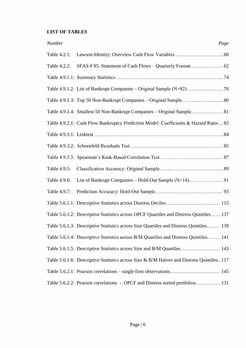
LIST OF TABLES
Number Page
Table 4.2.1: Lawson-Identity: Overview Cash Flow Variables ……………………….. 60
Table 4.2.2: SFAS # 95: Statement of Cash Flows – Quarterly Format……………….. 62
Table 4.9.1.1: Summary Statistics………………………………………………………... 74
Table 4.9.1.2: List of Bankrupt Companies – Original Sample (N=82)…………………. 76
Table 4.9.1.3: Top 50 Non-Bankrupt Companies – Original Sample………………......... 80
Table 4.9.1.4: Smallest 50 Non-Bankrupt Companies – Original Sample………………. 81
Table 4.9.2.1: Cash Flow Bankruptcy Prediction Model: Coefficients & Hazard Rates… 82
Table 4.9.3.1: Linktest …………………………………………………………………… 84
Table 4.9.3.2: Schoenfeld Residuals Test………………………………………………... 85
Table 4.9.3.3: Spearman’s Rank-Based Correlation Test……………………………….. 87
Table 4.9.5: Classification Accuracy: Original Sample..…...………………..……........ 89
Table 4.9.6: List of Bankrupt Companies – Hold-Out Sample (N=14)..………………. 91
Table 4.9.7: Prediction Accuracy: Hold-Out Sample………………………………….. 93
Table 5.6.1.1: Descriptive Statistics across Distress Deciles…………………………… 115
Table 5.6.1.2: Descriptive Statistics across OPCF Quartiles and Distress Quintiles…… 137
Table 5.6.1.3: Descriptive Statistics across Size Quartiles and Distress Quintiles…….. 139
Table 5.6.1.4: Descriptive Statistics across B/M Quartiles and Distress Quintiles…….. 141
Table 5.6.1.5: Descriptive Statistics across Size and B/M Quartiles…………………… 143
Table 5.6.1.6: Descriptive Statistics across Size & B/M Halves and Distress Quintiles.. 117
Table 5.6.2.1: Pearson correlations – single firm observations………………………… 145
Table 5.6.2.2: Pearson correlations - OPCF and Distress sorted portfolios…………… 131
Page | 7
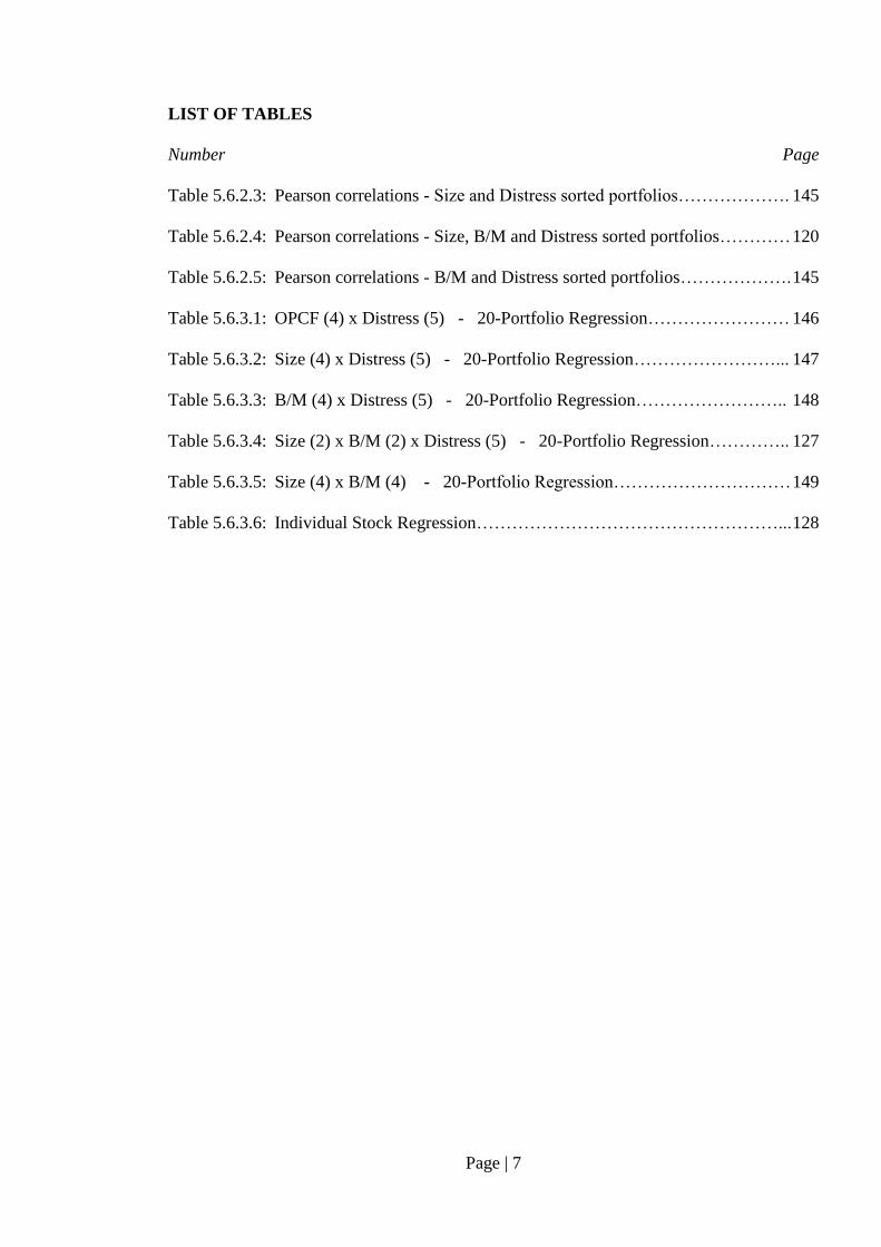
LIST OF TABLES
Number Page
Table 5.6.2.3: Pearson correlations - Size and Distress sorted portfolios………………. 145
Table 5.6.2.4: Pearson correlations - Size, B/M and Distress sorted portfolios………… 120
Table 5.6.2.5: Pearson correlations - B/M and Distress sorted portfolios………………. 145
Table 5.6.3.1: OPCF (4) x Distress (5) - 20-Portfolio Regression…………………… 146
Table 5.6.3.2: Size (4) x Distress (5) - 20-Portfolio Regression……………………... 147
Table 5.6.3.3: B/M (4) x Distress (5) - 20-Portfolio Regression…………………….. 148
Table 5.6.3.4: Size (2) x B/M (2) x Distress (5) - 20-Portfolio Regression………….. 127
Table 5.6.3.5: Size (4) x B/M (4) - 20-Portfolio Regression………………………… 149
Table 5.6.3.6: Individual Stock Regression……………………………………………... 128
Page | 8
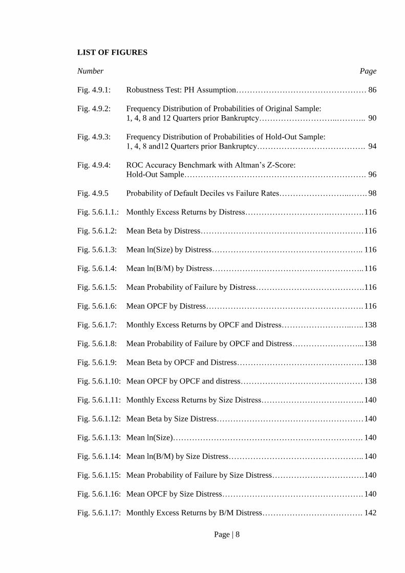
LIST OF FIGURES
Number Page
Fig. 4.9.1: Robustness Test: PH Assumption………………………………………… 86
Fig. 4.9.2: Frequency Distribution of Probabilities of Original Sample:
1, 4, 8 and 12 Quarters prior Bankruptcy………………………..……….. 90
Fig. 4.9.3: Frequency Distribution of Probabilities of Hold-Out Sample:
1, 4, 8 and12 Quarters prior Bankruptcy…………………………………. 94
Fig. 4.9.4: ROC Accuracy Benchmark with Altman’s Z-Score:
Hold-Out Sample…………………………………………………………. 96
Fig. 4.9.5 Probability of Default Deciles vs Failure Rates……………………..……. 98
Fig. 5.6.1.1.: Monthly Excess Returns by Distress………………………….…………. 116
Fig. 5.6.1.2: Mean Beta by Distress…………………………………………………… 116
Fig. 5.6.1.3: Mean ln(Size) by Distress……………………………………………….. 116
Fig. 5.6.1.4: Mean ln(B/M) by Distress……………………………………………….. 116
Fig. 5.6.1.5: Mean Probability of Failure by Distress…………………………………. 116
Fig. 5.6.1.6: Mean OPCF by Distress…………………………………………………. 116
Fig. 5.6.1.7: Monthly Excess Returns by OPCF and Distress……………………..….. 138
Fig. 5.6.1.8: Mean Probability of Failure by OPCF and Distress……………………... 138
Fig. 5.6.1.9: Mean Beta by OPCF and Distress……………………………………….. 138
Fig. 5.6.1.10: Mean OPCF by OPCF and distress……………………………………… 138
Fig. 5.6.1.11: Monthly Excess Returns by Size Distress……………………………….. 140
Fig. 5.6.1.12: Mean Beta by Size Distress……………………………………………… 140
Fig. 5.6.1.13: Mean ln(Size)……………………………………………………………. 140
Fig. 5.6.1.14: Mean ln(B/M) by Size Distress………………………………………….. 140
Fig. 5.6.1.15: Mean Probability of Failure by Size Distress……………………………. 140
Fig. 5.6.1.16: Mean OPCF by Size Distress……………………………………………. 140
Fig. 5.6.1.17: Monthly Excess Returns by B/M Distress………………………………. 142

Page | 9
LIST OF FIGURES
Number Page
Fig. 5.6.1.18: Mean Beta by B/M Distress…………………………………...………… 142
Fig. 5.6.1.19: Mean ln(Size) by B/M Distress………………………………………….. 142
Fig. 5.6.1.20: Mean ln(B/M)…………………………………………………………… 142
Fig. 5.6.1.21: Mean Probability of Failure by B/M Distress…………………………… 142
Fig. 5.6.1.22: Mean OPCF by B/M Distress…………………………………………… 142
Fig. 5.6.1.23: Monthly Excess Returns by Size………………………………………… 144
Fig. 5.6.1.24: Mean Beta by Size B/M………………………………………………….. 144
Fig. 5.6.1.25: Monthly Excess Returns by B/M………………………………………… 144
Fig. 5.6.1.26: Mean OPCF by Size B/M……………………………………………….. 144
Fig. 5.6.1.27: Mean Probability of Failure by B/M…………………………………….. 144
Fig. 5.6.1.28: Mean Probability of Failure by Size……………………………………. 144
Fig. 5.6.1.29. Monthly Excess Returns by Size, B/M and Distress…………………….. 118
Fig. 5.6.1.30. Mean Probability of Failure by Size, B/M and Distress…………………. 118
Fig. 5.6.1.31. Mean Beta by Size, B/M and Distress…………………………………… 118
Fig. 5.6.1.32. Mean OPCF by Size, B/M and Distress…………………………………. 118
Fig. 5.6.1.33. Monthly Excess Returns of Positive and Negative OPCF by Distress….. 119
Page | 10
The University of Manchester
Michael Kregar
Doctor of Business Administration
July 2011
Cash Flow Based Bankruptcy Risk and Stock Returns in the
US Computer and Electronics Industry
ABSTRACT
This thesis investigates the anomalous underperformance of distressed stocks in the US
computer and electronics industry. It shows that such anomaly can be explained by a
parallel analysis of risk based rational pricing and profitability (earnings) levels to returns
relationship propositions. For the 1990 to 2006 period, distressed stocks have on average
underperformed their non-distressed counterparts. However, once the conditional
relationship with profitability is taken into account, the distress risk is rewarded by a
continuous positive return hence priced appropriately.
In the computer and electronics industry growth stocks (low B/M) outperform on average
value stocks (high B/M). The size factor has not been confirmed to be significant in
explaining stock returns for this specific industry over the 1990 to 2006 period.
The study also reveals that B/M and size factors do not proxy for distress risk. The B/M
factor follows an inverted u-shape along the distress risk deciles axis. As result, stocks in
low and high distress portfolios share similarly low B/M values.
Cash flow based bankruptcy predictors estimated on a quarterly basis from a Cox
proportional hazard model, that are used as proxy for a continuous distress risk factor in
asset pricing tests, are able to predict bankruptcies at higher accuracy rates than the Z-
Score as alternative measure.

Page | 11
DECLARATION
I declare that no portion of the work referred to in the thesis has been submitted in support
of an application for another degree or qualification of this or any other university or other
institute of learning.
Michael Kregar
COPYRIGHT STATEMENT
i. The author of this thesis (including any appendices and/or schedules to this thesis)
owns certain copyright or related rights in it (the “Copyright”) and he has given
The University of Manchester certain rights to use such Copyright, including for
administrative purposes.
ii. Copies of this thesis, either in full or in extracts and whether in hard or electronic
copy, may be made only in accordance with the Copyright, Designs and Patents
Act 1988 (as amended) and regulations issued under it or, where appropriate, in
accordance with licensing agreements which the University has from time to time.
This page must form part of any such copies made.
iii. The ownership of certain Copyright, patents, designs, trademarks and other
intellectual property (the “Intellectual Property”) and any reproductions of
copyright works in the thesis, for example graphs and tables (“Reproductions”),
which may be described in this thesis, may not be owned by the author and may be
owned by third parties. Such Intellectual Property and Reproductions cannot and
must not be made available for use without the prior written permission of the
owner(s) of the relevant Intellectual Property and/or Reproductions.
iv. Further information on the conditions under which disclosure, publication and
commercialisation of this thesis, the Copyright and any Intellectual Property and/or
Reproductions described in it may take place is available in the University IP
Policy (see http://www.campus.manchester.ac.uk/medialibrary/policies/intellectual-
property.pdf) , in any relevant Thesis restriction declarations deposited in the
University Library, The University Library’s regulations (see
http://www.manchester.ac.uk/library/aboutus/regulations) and in The University’s
policy on presentation of Theses.

Page | 12
ACKNOWLEDGMENTS
First and foremost, I wish to thank my supervisor Dr Jens Hölscher for his academic
and professional guidance, his great support and endless patience throughout the long DBA
process. I am grateful to all academic and administrative staff at the University of
Manchester who guided me through the coursework and research process.
Thanks also to Professor Dean Paxson, Professor Richard Taffler and Dr Vineet
Agarwal for their critical comments that also improved this dissertation.
I also want to thank Professor Karthik Ramanna and Professor Suraj Srinivasan who
were giving me the opportunity to work as a research associate at the Harvard Business
School. This has been a very rewarding and unforgettable experience.
I would like to thank in no particular order Marjan Kregar, Peter Ramseyer, all my
relatives of the Hümmerich and Kregar families, my colleagues of Neurotune AG where I
have been working during my studies and any person who has been involved in a positive
way before and during my doctoral studies.
However, most of all, I thank my one and only wife Simone for her love, extraordinary
patience, understanding and encouragement over this very long period of study – she
deserves my deepest gratitude. I am also particularly proud of our son Elliott, who was
born in the period of doctoral coursework. He gives me some other perspective of life and
a lot of joy. While the journey of DBA studies is about to end, I am also very much
looking forward to spending some wonderful time with the youngest, our beautiful
daughter Goldie.
This piece of work is dedicated to my wife Simone, my son Elliott and my daughter Goldie.
God bless you.
Page | 13
CHAPTER 1: INTRODUCTION
The pricing of distress risk has become a frequently researched topic in recent years.
Dichev (1998), Campbell, Hilscher and Szilagyi (2008), Agarwal and Taffler (2008) and
others find contrary to the distress factor hypothesis (Fama and French, 1992, 1993; Chan
and Chen, 1991) that high distress risk is not rewarded by higher but substantially lower
than average stock returns. They conclude that it is very unlikely that a risk based rational
pricing proposition could explain the anomalous underperformance of distressed stocks.
Instead, they rather believe in a market underreaction hypothesis with respect to the pricing
of distress risk and find potential answers in the field of behavioural finance.
In this study, I will be able to show that a parallel analysis of two propositions, the risk
based rational pricing and the profitability/earnings levels to returns relationship can
explain the average underperformance of such distressed stocks. When the conditional
relationship with profitability is taken into account, the distress risk is rewarded by a
continuous positive return and is found to be priced appropriately.
There is an extensive body of accounting literature that discusses the theory and empirical
research on the relation between profitability reflected by earnings or cash flow
information and stock returns (Ball and Brown, 1968; Easton and Zmijewski, 1988; Easton
and Harris, 1991; Dechow, 1994, Beaver, 1998; and others). Several studies have
documented that it is not only the changes in earnings but also the level of earnings that
significantly and positively relate to stock prices (Easton and Harris, 1991; Penman, 1991,
Ohlson and Shroff, 1992). Therefore, firms generating higher earnings or cash flow levels
are also expected to earn higher average returns. In parallel, following a classical risk
based rational pricing model like CAPM or its derivatives such as a Fama and French
(1992) three-factor model, investors would expect a positive distress risk premium reward
hence higher average stock returns for riskier investments.
Given the two propositions above, investors would expect higher average returns when
investing in highly profitable but distressed stocks. However, for less profitable or even
loss making companies that are highly distressed, the same investors may still expect to
earn a distress risk premium but with a downward adjustment due to the lack of value
prospects as proxied by low or negative earnings or operating cash flows. In other words,
Page | 14
an investor or analyst may not only want to know the future payoff but also the risk as well
as the conditionality between the two factors involved.
The approach of this study is twofold from a risk of failure and pricing point of view. The
study focuses on and is limited to the industry “US Computer and Electronic Product
Manufacturing”, which is one with the highest number of companies operating under
permanent distress in the United States. In 2004, there were about 300 firms, which on
average represent approximately 35% of this industry, operating under distress and facing
a potential bankruptcy (PricewaterhouseCoopers, 2006). In 2005, there were 80 public
companies filing Chapter 11, whereof 29 of these bankruptcies were related to the
computer equipment and machinery manufacturing industry with assets at filing of $ 23.9b.
As shown in previous research (Campbell, Hilscher and Szilagyi, 2008; Agarwal and
Taffler, 2008), distress risk values used in asset pricing tests are often proxied by
bankruptcy risks obtained from a bankruptcy prediction model. Therefore, the first part of
this study deals with the development of an industry specific cash flow based bankruptcy
prediction model, which is able to classify and predict the event of bankruptcy at a
relatively high level of accuracy. Most of the MDA or conditional probability models
(Altman, 1968; Ohlson, 1980; Taffler, 1983, 1984; Zavgren, 1983; Aziz, Emanuel, Lawson,
1988; Shumway, 2001; Campbell, Hilscher, Szilagyi, 2008 and others) found in previous
literature used publicly available financial statement and stock market data as well as other
non-financial information to segregate into failure and non-failure firms. A variety of
statistical methods and sets of accounting, market and non-accounting variables were
tested. Bankruptcy prediction models are widely used in the banking sector as well as in
other industries and provide some reasonable assessment on a firm’s risk of failure. A
detailed literature review on bankruptcy prediction models is provided in section 2.1.
The second group of research, which is found to a lesser extent in literature has become an
increasingly researched topic in recent years. It tests for the relationship between the
bankruptcy models’ derived distress risk and related stock returns. The risk factor used in
asset pricing tests is often proxied by the scores or probabilities derived from bankruptcy
prediction models such as from Altman’s (1968) Z-score, Ohlson’s (1980) O-Score or
more recently from a fitted probability model by Campbell, Hilscher and Szilagyi (2008).
Page | 15
The arguments for this relationship studies are that capital market agents in the aggregate
would use multivariate information from financial statements and market data condensed
in a bankruptcy prediction model and invest based on their given risk-return preferences.
The studies found in the accounting and finance literature include the testing of the
relationship between stock returns and bankruptcy risk, but also the market reaction from
an information efficiency point of view and do range from short-term event to long-term
association type of studies. Dichev (1998), Campbell, Hilscher and Szilagyi (2008),
Agarwal and Taffler (2008) and others find contrary to the distress factor hypothesis of
Fama and French (1992, 1993) or Chan and Chen (1991) that high bankruptcy risk is not
rewarded by higher but substantially lower than average stock returns. They conclude that
it is very unlikely that a risk based rational pricing proposition could explain the
anomalous underperformance of distressed stocks. Instead, they rather believe in a market
underreaction hypothesis with respect to the pricing of distress risk and find potential
answers in the behavioural field of finance. A literature review on the pricing of distress
risk is provided in section 2.2.
The study consists of two main parts. In the first part (Chapter 4), I have constructed a
dynamic cash flow based bankruptcy prediction model in order to obtain probabilities of
failure on a firm by firm basis. The predictors estimated on a quarterly basis using four-
quarter accumulated financial statement data have the distinct advantage of pre-empting
the information content provided by annual models. This industry specific model uses in
contrast to many other studies non-arbitrarily selected cash flow variables that are
calculated based on Lawson’s Cash Flow Identity (Lawson, 1971) using financial data
from the statement of cash flows as required by the Statement of Financial Accounting
Standards (SFAS) No. 95. The model therefore relies on publicly available financial
statement data only and does not incorporate any equity market data as predictors in
contrast to most of other models. This econometric model is constructed on the grounds of
one of the more recent developments in this field by employing a hazard model (Shumway,
2001; Beaver, McNichols and Rhie, 2004; Campbell, Hilscher and Szilagyi, 2008). Since
bankruptcy probabilities vary over time, a hazard model may produce more efficient and
time-varying out-of-sample forecasts and as such may result in stronger association with
stock returns (Shumway, 2001). Therefore, the cash flow predictors are estimated on a
quarterly basis using the Cox proportional hazard model (Cox, 1972). The model’s
Page | 16
prediction outcomes are validated by confirmative out-of-sample and favourable
benchmark test results over Altman’s Z-score using the receiver operating characteristic
measure and can be considered to be robust. This Cox proportional hazard model not only
predicts corporate failure, but also produces the probabilities of failure for each firm on
quarterly basis which serve as a proxy for the continuous relative distress risk factor to be
included in asset pricing tests.
The second part (Chapter 5) is dedicated to the pricing of the relative distress risk factor
derived from the bankruptcy prediction model’s probability of failure and the profitability
levels proxied by an operating cash flow variable. The study has foreseen several tests to
be conducted in order to accept or reject various hypotheses set in section 3.3, particularly
related to the parallel analysis of the risk based rational pricing and the
profitability/earnings levels to return relationship propositions.
The results of the hypotheses testing ought to provide answers with regards to the main
research question if the anomalous market underperformance to distressed stock can be
explained by the above mentioned parallel analysis and if a potential conditionality
between the distress risk and profitability factors exists. The descriptive statistics show that
on average, highly distressed stocks do underperform non-distressed firms. This finding is
consistent with Dichev (1998), Campbell, Hilscher and Szilagyi (2008) and Agarwal and
Taffler (2008). However, once the conditional relationship with profitability is taken into
account, the distress risk is rewarded by a continuous positive return. Two-thirds of highly
distressed companies in the computer and electronics industry have low or negative excess
returns and low or negative profitability levels. The other third of distressed companies is
profitable and earn superior returns compared to a) their non-distressed counterparts and b)
to distressed but non-profitable companies. I also provide Fama-MacBeth (1973) t-
statistics resulting from cross-sectional regressions run on several two-way and three-way
intersecting and independently sorted portfolios. The t-statistics confirm in a joint setting
the significance of the relative distress risk factor and current profitability levels, both
derived from the cash flow based bankruptcy prediction model. In addition, I separately
test for the potential conditionality of these two factors. Next, I conduct Pearson
correlation tests and also run Fama-MacBeth (1973) cross-sectional regressions for both
the distress risk and current profitability strength factors to see if they are independent
Page | 17
from the Fama-French (1992) factors. The tests confirm that both new factors are
independent from the Size and B/M factors. The descriptive statistics also reveal that the
B/M factor follows an inverted u-shape along the distress deciles axis, which means that
low and high distress risk deciles share similarly low B/M values. Furthermore, cross-
sectional regression results confirm that adding both the distress risk and profitability
strength factor improve the explanatory power over an initial Fama-French three-factor
model and also that both factors are not subsumed by Size or B/M. Given the correlation,
descriptive and inferential statistics’ test results I can prove that the Fama-French (1992,
1993) distress factor proposition does not hold.
What is the main contribution of this study? Overall, I can show that the anomalous
underperformance of distressed stocks in the US computer and electronics industry can be
explained by the parallel analysis of two propositions; the risk based rational pricing and
the positive relationship between profitability levels and stock returns. There is evidence
that distressed stocks are rewarded with a positive continuous distress risk premium and
appropriately priced once the conditionality with profitability is taken into account.
In addition, I present a dynamic cash flow based hazard model which predicts bankruptcies
at higher accuracy rates than Altman’s Z-score model as shown by a ROC model
benchmark test. This model not only predicts corporate failure, but also produces
probabilities of failure for each firm on quarterly basis which in turn serve as a proxy for
the continuous relative distress risk factor to be included in asset pricing tests.
The study also shows that the distress factor hypothesis as proposed by Fama and French
(1992) does not hold. Last but not least, growth stocks earn a higher premium than value
stocks in the computer and electronics industry hence it reflects the opposite of what Fama
and French (1992, 1993) have found for the market as a whole. This reversed effect of the
B/M anomaly may be explained by the fact that the computer and electronics industry was
growth oriented over this period of rapid technological advancement. Investors may have
awarded high multiples relative to the book equity for these industry-specific companies by
anticipating substantially higher future sales and earnings compared to the prevalent
fundamentals given at the time of investment.
Page | 18
CHAPTER 2: LITERATURE REVIEW
2.1 Past Research on Bankruptcy Prediction Models
2.1.1 Introduction
The bankruptcy rates have risen remarkably in an environment of increased globalization
and competition and as result causing very large direct (e.g. legal and accounting fees) and
even much larger indirect costs to the economy as a whole. Therefore, it is not a surprise
that the area of corporate failure prediction has become an important and popular area of
research over the last four decades. Although, the majority of bankruptcy filings are made
by private companies, most of the bankruptcy prediction studies predominantly focus on
publicly traded companies for the simple reason of mandatory disclosure requirements of
financial statement data (in the United States, 224,472 companies filed for Chapter 11 from
1980 to 1991 of which about 1200 public ones were involved (Altman, 1993). In the years
from 1992 to 2005, another 1700 public firms have filed for Chapter 11, which is on
average about 120 filings per year (PricewaterhouseCoopers, 2006). The
PricewaterhouseCoopers’ Phoenix Report from 2005/2006 also shows the materiality of
bankruptcy with respect to total assets at the time of filing, which was $ 101.3 billion in
2005. The event or the risk of business failure may affect many parties (debtor,
government, creditors, auditors, investors, turnaround specialists etc), either directly or
indirectly.
Many researchers have constructed models with the aim to predict the failure or non-
failure of distressed companies using all kind of variables such as financial ratios from
financial statements, market-derived indicators, cash flow ratios, economic and industry
specific indicators and many more in an endless number of combinations. One of the first
bankruptcy prediction models, if not the first, was developed by Beaver (1966) which
included a full set of financial ratios deriving from publicly available financial statements.
Beaver (1968) used the univariate analysis (section 2.1.3.1), a single-period statistical
method, which then was followed by some other multivariate models. The most popular
statistical methods appear to be the cross-sectional ones such as the multivariate
discriminant model (MDA). It was introduced by Altman (1968) and has been used for
many years and in the 1980, it was followed by logit models (LA) (Ohlson, 1980). Another
conditional probability model, the probit analysis (PA) has been introduced by Zmijewski
(1984), but has not become as popular as the logit analysis in the application of bankruptcy
Page | 19
prediction models (Balcaen and Ooghe, 2006). More recent, Shumway (2001) has
introduced a simple hazard model which in contrast to static models mirrors the dynamic
event of company failure much closer than any of the previous models.
Further below, I will first discuss some issues on failure and bankruptcy definitions, then
describe some of the most popular statistical methods which were applied in past studies
and I will also cover some methodological related issues or pitfalls.
2.1.2 Definition of “Firm’s Bankruptcy or Failure”
The failure of firms can be understood in many different ways such as from an economical
and legal or from a static and dynamic point of view. Expressions like failure, bankruptcy,
corporate distress, insolvency, default and others are found in the literature and are very
often used interchangeably in the same context without a clear distinction of meaning.
Altman (1993), Balcaen and Ooghe (2006), Karels and Prakash (1987) and others provide
some overview of corporate distress definitions. The first expression “economic failure”
can be identified by net losses incurred or by lower average return on investments
compared to alternative investments, which however do not ultimately lead to a
discontinuation of a firm’s operation (Laitinen, 1994). As such there is no single or specific
event of failure from an economical point of view, but it is rather an occurrence over time.
The second expression, an “insolvency issue” is found when a company cannot meet their
financial obligations. However, insolvency also does not have to lead to a liquidation or
discontinuation of a firm either and as such is also not considered to be a good indicator of
distinction between failed or non-failed companies from a shareholders’ total loss
perspective. The next definition used, “defaults” as explained by Altman (1993), is also not
a clear-cut event of bankruptcy and may not lead to a significant loss of shareholder’s
investment by liquidation. Defaults such as violation of covenants can be an indication of
shortfall in cash generation and lack of liquidity, but are very often restructured with bank
syndicates and therefore may continue their operations (Altman, 1993). Last but not least,
the term bankruptcy, which is understood to be a legal act such as the filing under Chapter
11 in the United States is probably the best indicator of a company facing potential
liquidation, but varies from country-to-country depending on their national bankruptcy
codes. The bankruptcy term viewed as a legal act such as in the United States is the most
often used criteria and common choice in the bankruptcy prediction literature. It is

Page | 20
considered to be the “real” event when selecting bankrupt and non-bankrupt firms for
modelling and testing purpose (Karels and Prakash, 1987).
This so-called “real” event has also some serious pitfalls to consider. One is that a chapter
11 filing may be done on a voluntary basis in order to prevent a firm’s liquidation by a
successful reorganization which in turn may not result in the discontinuation of a company
at all. Therefore, it may not be classified as a genuine company failure in any model.
It is quite essential that the event of failure or bankruptcy is precisely defined and
adequately incorporated in the design of a research project, which has not always been the
case in past studies (Karels and Prakash, 1987). The omission of such a definition weakens
the models’ design and validation. Moreover, it may result in an arbitrary selection process
of non-failure and failure companies (more about the arbitrary separation of populations;
see dichotomous dependent variable section 2.1.4.4)
2.1.3 Statistical Methods Used in Bankruptcy Prediction Studies
2.1.3.1 Univariate Analysis
The univariate (discriminant) analysis has been used to create a bankruptcy prediction
model based on financial ratios. It has been introduced in the 1960 by Beaver (1966, 1968),
the pioneer in the studies of bankruptcy prediction models. He found that a number of
ratios or indicators of a paired sample of failed and non-failed companies could predict
company failure for a period of up to five years before such negative event actually occurs.
Basically, he has been identifying the ratios by applying a dichotomous classification test
and as result obtained the final set of six ratios of which of each had the best ability to
predict the companies’ failure. In his test, firms from a paired sample of 79 distressed and
79 non-distressed firms have been matched by asset size and industry (issues on sample
selection, see section 2.1.4.3). Each ratio in the model was measured and analysed on a
one-by-one basis against an “optimal cut-off point” – this is the value to be set in order to
reach the lowest percentage of misclassifications. If a company’s ratio value was below
this so-called “cut-off point” it was considered to be a failing company, if its ratio value
was found above the point, it was classified as non-failing. The model with its cut-off point
has also been tested against a hold-out sample, a sample not been part of the model itself
Page | 21
(validation; ex ante). The classification accuracy was measured by a total misclassification
rate, which itself was split into type I and type II errors. Type I error was found when a
company was classified as non-failed, but in reality failed and the type II error was found
when a company was classified as failed, but did not fail.
Since the cost of type I and type II errors are not considered to be the same, the optimal
cut-off point can be modified in order to achieve lowest error rates (Zavgren, 1983). In
brief, the obvious advantage of Beaver’s univariate analysis based model as concluded by a
majority of researchers in this field is that it does not require any special statistical
knowledge, but still provides a remarkably high predictive ability. It is a simple manual
process of comparing ratio values with the cut-off point which in turn classifies firms into
failed or non-failed.
However, the univariate analysis also has some serious constraints. The method works
under the assumption of linear relationship between ratios and the outcome such as failure
or non-failure. Studies have shown that most of the financial ratios relate in a non-linear
manner. Second, the ratios are measured on a one-by-one basis (univariate) and may create
some inconsistent result among the ratios. Third, most variables or ratios are highly
correlated (Zavgren 1983) and therefore, it is also very difficult to assess the significance
of ratios on an individual basis. Fourth, it is also quite obvious that a firm’s financial
condition is more likely to be assessed on the combination of multiple ratios rather than on
a single ratio’s outcome, which has led Altman (1968) to use the multiple discriminant
analysis in order to overcome this deficiency (section 2.1.3.2). Last but not least, the
optimal cut-off points for each variable are sample specific and trial-and-error based and as
such may result in higher errors rates when conducting ex ante out-of-sample tests (Platt
and Platt, 1990). Overall, the univariate analysis is no longer of relevance when
considering the advantages of the models discussed in the next sections.
2.1.3.2 Multiple Discriminant Analysis (MDA)
Altman (1968) used the multiple discriminant analysis as statistical method, which allows
classifying firms into two or more a priori groups such as failure or non-failure companies.
His failure prediction model is called “Z-score model” and has been adjusted by the
ZETA-analysis (Altman, Haldeman, Narayan 1977) in order to reflect the changes in
Page | 22
accounting and reporting standards (ZETA-Model will not be discussed in further details).
In contrast to the univariate analysis, it combines the ratios and “it attempts to derive a
linear combination of these characteristics, which “best” discriminates between the groups”
(Altman, 1968). In the 1970, it has been the most frequently applied method in the
literature (Deakin, 1972; Edmister, 1972; Taffler and Tisshaw, 1977) and is still widely
used and accepted.
The MDA is based on Lachenbach’s (1975) linear discriminant function:
Di = D0 + D1Xi1 + D2Xi2 + …. + DnXin
with Di = discriminant score for firm i
Xij = value of the attribute Xj (with j = 1, , n) for firm i
Dj = linear discriminant coefficients with j = 0, 1, , n
The researcher’s inputs are variables or ratios which he believes will discriminate best
between the two a priori groups, failure and non-failure. In contrast to the univariate
analysis, variables may be included in a MDA model, which would not have been
considered to be a best predictor when evaluating them individually for statistical
significance. For this reason, Beaver’s (1966) set was not identical with Altman’s (1968)
five variables. The MDA model brings the multi-dimensional input of selected ratios into a
one-dimensional measure by forming a linear combination of the variables along some axis.
The MDA determines the linear combination n attributes (financial ratios) with the widest
separation of means and as such is providing the best discriminator between groups in the
form of a score (Di). I will not go into more details regarding the complex computations of
an MDA model (further discussion see Zavgren (1984)).
As found when using the univariate analysis, Altman (1968) determined an optimal cut-off
point or score in order to obtain the lowest error rates (type I and type II errors as discussed
in the previous section). The Altman (1968) test included thirty-three manufacturers that
filed bankruptcy and another equal number of non-bankrupt manufacturing firms, which
were matched by asset size and industry for one year prior bankruptcy. The classification
accuracy of the model has also been assessed on an overall as well as on a type I and type
Page | 23
II error basis. The result shows that Altman’s (1968) model achieved a higher accuracy on
year one prior bankruptcy (95%) than Beaver’s (1966) univariate model. However,
Beaver’s model was more accurate in the years three to five prior bankruptcy. Nevertheless,
the multivariate analysis is still intuitively more convincing than the univariate analysis.
All researchers would most likely doubt that one single ratio was able to capture more
complete information than a set of ratios reflected in a single Z-score (Zavgren, 1983).
Altman’s discriminant function was validated by using the same firms, but with ratios
drawn from years two to five prior bankruptcy. Moreover, another sample with twenty-five
distressed firms was tested based on the initially obtained coefficients in order to validate
the predictive power of the model (ex ante). The test results of the out-of sample test
showed some significant increase in type I error rate though.
Although, the multiple discriminant analysis has brought some improvements over the
univariate analysis, there are quite some restrictions and issues to be considered when
using the MDA as statistical method. The MDA requires that (Karels and Prakash, 1987):
a) the groups (dependent variables) are dichotomous (discussion see section 2.1.4.4)
b) the independent variables are multivariate normally distributed
c) variance-covariance matrices are equal across both groups of classification
d) the prior probability of failure and misclassification costs are specified
In practice, the requirements above are very often violated (Eisenbeis, 1977; Richardson
and Davidson, 1984; Zavgren 1983). Almost none of the studies including the ones I have
reviewed ever analyse whether or not they meet the above requirements (Balcaen and
Ooghe, 2006). Therefore, the generalizations and conclusions in these studies may be
somewhat questionable.
Financial ratios, also the ones used as independent variables in MDA models, are not
normally distributed (Barnes, 1982) and therefore require some correction such as log
transformation (Altman, Haldeman, Narayan 1977), quadratic transformation of variables
(Joy and Tollefson, 1975) or other types of transformation. Some researchers may have
chosen to eliminate outliers by deletion (Frecka and Hopwood, 1983) or windsorising as a
Page | 24
widely used alternative. In general, I conclude that the multivariate normality assumption
should be satisfied by one of the available remedies as suggested in the literature.
Another issue is the selection of an optimal cut-off score based on the assumption of
minimized cost function. Type I and Type II errors are not equal from a cost point of view.
From an investment banker’s point of view, a type I error is significantly more costly than
a type II error (loss of loans etc). However, from a mistakenly classified non-failed firm,
the cost of type II error would be higher because of wrong signalling to creditors,
customers, stockholders and other stakeholders (Zavgren, 1983). This can lead to
significant opportunity costs, which however are almost immeasurable. For practical
reasons, most, if not all, of the studies assume cost equality for both, type I and II error,
with the result of an incorrect and biased setting of the “optimal” cut-off point. (Zavgren
1983). One solution is to specify lower and upper cut-off scores by achieving a zero per
cent type I at the upper as well as a zero per cent type II error rate at the lower cut-off score
point – the so-called “black-grey-white”-method (Edmister, 1972).
Another disadvantage is the fact that the MDA works on the assumption of linear
relationship between the dependent dichotomous and the independent variables. Balcaen
and Ooghe’s (2006) point out that most of the variables such as financial ratios do not
relate linearly to the financial condition of a company. The logit analysis, with a non-linear
maximum likelihood estimator is a more appropriate method and can overcome this quite
serious deficiency (see section 2.1.3.3).
Financial ratios among themselves are very often correlated by sharing the same
denominator or nominator. Therefore, one would have to expect some issues regarding
multicollinearity. However, Altman and Eisenbeis (1978) concluded that there is no such
problem in the use of an MDA model, which definitely would pose an advantage over the
logit analysis (see section 2.1.3.3.).
The introduction of the MDA model was an important milestone in the history of
development of bankruptcy prediction models. Nevertheless, the disadvantages compared
to the logit analysis and the following discussion will show why the MDA has frequently
become a second choice of method in the literature.
Page | 25
2.1.3.3 Logit Analysis (LA)
In the 1980, the logit analysis (LA), a conditional probability model, which was introduced
by Ohlson (1980), became one of the most popular statistical methods in the failure
prediction literature. The LA is a non-linear maximum likelihood estimation procedure:
P1(Xi) = 1 / [1 + exp –(B0 + B1Xi1 + B2Xi2 + … + BnXin)] = 1 / [1 + exp –(D1)]
with P1(Xi) = probability of failure given the vector of attributes Xi
Bj = coefficient of attribute j with j = 1, , n and B0 = intercept
Xij = value of the attribute j (with j=1, ,n) for firm i
Di = the “logit” for firm i
When a failed company is coded with 1 and the logit score results in a high P that means
that there is a high probability of failure and vice versa. The logit analysis works based on
“resemblance principle” as the MDA method does (Balcaen and Ooghe, 2006). The
optimal cut-off point of the logit score (P1Xi) has been assessed in Ohlson’s (1980) study
based on the same assumption as in Altman’s (1968) study; to minimize the total cost of
error assuming cost equality for type I and type II errors.
The result of Ohlson’s (1980) and also Zavgren’s (1982) studies did not show any
improvement in the accuracy of classification compared to Altman’s (1968) and other
authors’ MDA based models. However, there are still some distinct advantages over the
MDA methods to be taken into account when selecting the appropriate statistical method.
The logit analysis does not require normally distributed variables or equal dispersion
matrices or prior probabilities of failure as MDA does (Ohlson, 1980; Zavgren, 1983). The
logit analysis provides direct information on probabilities of failure as reflected by its logit
score (P1Xi), and as such is viewed as “the main contribution of this [LA] technique”
(Zavgren, 1983). In addition, the estimated coefficients derived from a LA model can be
evaluated for each independent variable separately regarding its statistical significance and
its contribution to the model as a whole (Zavgren, 1983; Ohlson, 1980). This feature is not
available with the MDA model (see section 2.1.3.2). Last but not least, the logit analysis
works based on a non-linear maximum likelihood procedure, which overcomes the
Page | 26
problem of non-linear relationship among variables as discussed with the MDA method
(section 2.1.3.2).
Although, the LA model appears to be less restrictive and also less complicated than a
MDA model, there are also some serious limitations discussed in the literature. One
problem, which potentially could arise, is multicollinearity among independent variables
since financial ratios have quite often the same numerator or denominator, a serious
drawback of which the MDA is not subject to (section 2.1.3.2). Although, the LA model
does not require normally distributed variables, it is still sensitive to extreme non-
normality and to outliers as well as missing values (McLeay and Omar, 2000). Therefore,
transformation including outlier deletion is recommended in order to obtain close to
normality distribution (Balcaen and Ooghe, 2006) and may also be advisable when using
the LA method (see discussion in section 2.1.3.2).
Overall, I conclude that for simple dichotomous classification into failing or non-failing
group, the MDA model may still be the most appropriate method. The logit analysis has
some clear advantage over the MDA model when it comes to the assessment of likelihood
of failure (probabilities). In addition, the non-linear shape of LA method in contrast to
MDA’s linear functionality is quite appealing and avoids the transformation of variables
(logs and quadratic terms).
2.1.3.4 Hazard Model – Cox Proportional Model
One of the more recent developments in this field is the application of a hazard model,
which has been introduced by Shumway (2001) and which has been used by other
researchers recently such as Beaver, McNichols and Rhie (2004) or Campbell, Hilscher
and Szilagyi (2008). All previous models as discussed above are single-period or static
models, which do not account for changes of a firm’s characteristics over time. The static
models typically are created by using financial data from one year prior to bankruptcy. In a
second step, the researchers run their models for years two to five prior bankruptcy with
coefficients obtained from year one and as result ignore any time varying characteristics of
failing firms. In other studies, researchers create year specific models from t-1 to t-5
(multiperiod logit models) and use them as separate observations not linked to each other
over time. Therefore, Shumway (2001) claims that all static models (MDA and LA) are
Page | 27
inappropriate for forecasting bankruptcy. He suggests the use of a hazard model in
connection with a logistic model, also known as survival or duration analysis, as the most
adequate statistical method in this field. Although, Shumway (2001) has proven that logit
and hazard models are closely related to each other, he provided some distinct advantages
of a hazard model from an econometric point of view:
a) it accounts for time unlike static models as discussed earlier. The dependent variable in
a hazard model is the time spent by a firm in a healthy group
b) bankruptcy probability varies over time. Circumstances may change that influence the
probability of an individual firm facing bankruptcy. In effect, Kiefer (1988) says the
conditional probability of exiting a state is not constant over time, a factor which by
definition is not considered in a single-period model at all.
c) automatic adjustment for period at risk; some firms file bankruptcy while being at risk
in the first year and others maybe after five or more years. Other companies may file
bankruptcy without being at risk at all (voluntary filing)
d) it incorporates time-varying explanatory variables
e) it produces more efficient out-of-sample forecasts by utilizing more data than static
ones.
Shumway (2001) also admits that hazard models are difficult to estimate due to their non-
linear likelihood functions and time-varying covariates and basically refers to computer
programs estimating hazard rates based on logistic estimation models. His work revealed
that more than half of previously used accounting ratios were statistically not significant
and as such he proposed a model that uses a very limited number of both accounting ratios
and market-driven variables combined. The fact that a hazard model does account for time-
series behaviour of variables is very much appealing since company failure may most
likely occur over multiple periods and as such cannot be captured just by a snap-shot of a
single annual financial statement. Nevertheless, hazard models are also sensitive to
extreme outliers as well as missing values, an issue which can be solved as discussed under
2.1.3.3. The hazard model offers the probability of failure directly, which is not given by
the MDA method (2.1.3.2) and also incorporates time-varying variables (aspect of panel
data analysis), which is not given by the logit analysis (2.1.3.3). Therefore, I consider it as
Page | 28
the most appropriate method to be used for developing the cash flow based bankruptcy
prediction model as described in Chapter 4.
One of the most popular and widely-used hazard model is the Cox proportional hazards
regression method (Cox 1972), a relative risk model. It is a semi-parametric model, which
means that it does no more than analyzing the combined individual binary-outcome at each
time of potential failure. The binary outcome in this study is either bankrupt = 1 or non-
bankrupt = 0. The Cox proportional hazards regression model (Cox 1972) asserts that the
hazard rate h at time (t) for the jth subject in the data x is
h(t|xj) = h0(t) exp(xj x)
The h0(t) is the baseline hazard, which has no parameterization and as such will not be
estimated. Hence, this model does not make any assumption about the shape of the hazard
over time and does not rely on distributional assumptions in contrast to other methods as
discussed above (parametric part of the model). This is an important feature since the
distribution cannot be specified. As result, the Cox model overcomes the violation of non-
normality distribution and produces more efficient and robust results. The x regression
coefficients are to be estimated from the data xj. The Cox model assumes a parametric
form for the effect of the predictors on the hazard (non-parametric part of the model) and
since this study is rather interested in the parameter estimates than the shape, the Cox
model is considered to be the most appropriate choice of method. If the functional form of
h0(t) was known, parametric models such as Weibull or Exponential regression could have
been chosen depending on the data’s shape . Nevertheless, a wrong assumption about the
distribution could then produce misleading results.
To obtain a bankruptcy prediction model by the application of the Cox proportional hazard
model one needs to, besides structuring the data properly, consider the following:
a) The Cox model has no intercept since it is equal to the baseline h0(t) and as discussed
does not built on the distribution shape of the data used.
Page | 29
b) The interpretation of the hazard rate which results from the exponentiated individual
coefficient is relatively easy. Nevertheless, a hazard rate is not a probability p and
therefore, needs to be calculated as follows:
Since, I would like to obtain the probability of failure for a single company with multiple
covariates at a given quarter; I use the STATA “predict hr” function after running the Cox
regression. This function will provide the overall hazard rate (hr) on an observation by
observation basis within-sample, but also allows to be re-run out-of-sample for validation
purpose. The probability of failure derived from a hazard model can be viewed as an
equivalent to a discrete time multi-period logit model as shown by equation below:
where pi,t stands for the probability that firm i will be bankrupt at time t , e for Euler’s
constant at 2.7183 and –z for 1x
1 +
2x
2 + …..+
px
p.
c) The Cox proportional hazard model is sensitive to the problem of multicollinearity.
Therefore, the variables used for modelling will need to be evaluated by a correlation
test. Strong correlations among independent variables should be avoided (Lane,
Looney, Wansley 1986).
d) As with any other regression method, the Cox model’s result needs to be checked for
eventual misspecifications, outliers etc (Cleves, Gould, Gutierrez 2003).

Page | 30
2.1.4 Common Statistical and Methodological Issues
2.1.4.1 Selection of Independent Variables
No theoretical framework has been identified in existing bankruptcy literature, which could
provide knowledge about the variables to be selected when building or testing a
bankruptcy prediction model (Zavgren 1983). Therefore, many different set of variables
can be found in the literature such as accounting, market-related or non-financial ratios
based models in all kind of combinations. Most of the researchers in this area run empirical
tests based on a number of different statistical methods and chose the variables of
significance. Others take an existing model with a given set of variables obtained by
previous research work and studies. In the past four decades, dozens of ratios have been
tested and used in numerous bankruptcy prediction models without any underlying theory
by some of the most prominent researchers in that field.
2.1.4.2 Lawson-Identity
Nevertheless, one study on bankruptcy prediction was conducted by using a framework for
the selection of independent variables. Aziz, Emanuel and Lawson (1988) have obtained a
set of cash flow related variables based on Lawson’s cash flow identity (Lawson, 1971),
which in sum can be described as follows:
Entity Cash Flows = Lender Cash Flows + Shareholder Cash Flows
The entity cash flow is the sum of the following:
Entity Cash Flows = Operating Cash Flow
./. Net Investment in Fixed Assets
./. Liquidity Changes – Taxes paid
Thus, the cash flow information derived from this identity includes operating cash flow,
net capital investment, liquidity change, taxes paid on the left side and lender as well as
shareholder cash flows on the right side of the equation as shown below (Aziz, Emanuel,
Lawson 1988):
(kj – hj) - (Aj + Rj – Yj) – Hj – tj = (Fj – Nj – Mj) + (Dj – Bj)
Page | 31
where,
kj – hj is operating cash flow in year j (customer cash payments, kj, less
operating cash flow, hj
Aj + Rj – Yj represents net capital investments as result of replacement investment, Aj,
plus growth investment, Rj, less the proceeds from asset disposals, Yj, in
year j
Hj reflects the change in liquidity in year j
Tj for taxes assessed and paid in year j
Fj represents interest payments in year j
Nj is medium and/or long term debt raised or retired in year j
Mj is short-term debt raised or repaid in year j
Dj is dividends paid to shareholders in year j
Bj represents equity capital raised or repaid in year j
Aziz, Emanuel and Lawson (1988) have tried to compare their cash flow based prediction
model (CFB) with widely and most accepted models such as Altman’s Z-Score and ZETA.
The overall accuracy of the CFB model was in year one, three, four and five prior
bankruptcy higher than the well known Z-Score, but lower in all years than the ZETA
model. However, the CFB model had some better accuracy rates in identifying bankrupt
firms than both ZETA and Z-Score in years three, four and five prior bankruptcy.
There are several pitfalls to consider when comparing different models as done by Aziz,
Emanuel and Lawson (1988). First, it is unclear whether these accuracy differences relate
to the selection of variables or the choice of statistical method. On one hand we have the Z-
Score which stems from the multiple discriminant analysis method and on the other hand a
cash flow based model using logit analysis. Second, the results from all these prediction
models derive from different periods and samples and as such produce rather non-meaning
comparisons. Third, Aziz’, Emanuel’s and Lawson’s (1988) model consists of annual
Page | 32
specific logit models, which means that for each year prior bankruptcy there is a specific
model with variables having different coefficients. This CFB model cannot be used for
hold-out sample tests since it is unclear which annual logit model’s coefficient one would
have to use. Last but not least, comparisons with other models can only hold if the same
hold-out sample at the same period is run by each model’s coefficients, which has not been
done by this CFB study. Nevertheless, Aziz, Emanuel and Lawson (1988) rightly argue
that corporate bankruptcy is closely related to a company’s valuation and as such the
Lawson’s cash flow identity variables are expected to be stronger predictors. Others such
as Ross, Westerfield and Jaffe (2002) also refer to flow-based insolvency, which occurs
when a company’s cash flow is insufficient to meet its financial obligation. Overall, it is
intuitively appealing to estimate identity based cash flow failure predictors from a hazard
proportional model using panel instead of cross-section data. That is the justification why I
will apply Lawson’s identity when developing a new bankruptcy prediction model. It is the
only non-arbitrary type of selection of variables using an identity, which I have found so
far in previous studies.
2.1.4.3 Sampling Method
In a perfect world, the sample drawn from a population should be representative for the
population of all firms. However, most of bankruptcy prediction studies including the ones
mentioned in this study are based on non-random sampling and therefore may be subject to
biased parameter estimates and probabilities (Zmijewski, 1984). As result, most if not all,
achieve remarkable results in within-sample classifications (ex post), but clearly fail when
it comes to their predictive ability by validating the models with out-of-sample
classification tests (ex ante). Platt and Platt (1990) analysed this issue and concluded that
so-called well predicting models typically experienced a disappointing shortfall of ten or
more percentage points from within-sample compared to out-of-sample classification test
results. A few studies such as from Platt and Platt (1990), Platt and Platt (1991) and Pompe
and Bilderbeek (2000) suggest the inclusion of industry-relative, size class specific or age
specific variables in order to improve the predictive power of failure models.
Another issue to be considered when assessing the classification accuracy of tests is the
“over-sampling” problem (Zmijewski, 1984). Bankrupt companies are selected based on
their known status of failure and represent a much higher proportion of the population than
Page | 33
in the real world, especially when using matched pairs of failing and non-failing companies
(fifty per cent failed; fifty per cent non-failed matched by asset size and industry). This
problem of choice-based sample bias (Zmijewski, 1984) leads to an overstatement of the
ex-post accuracy of classification results and to misleading conclusions (Platt and Platt,
2002). In contrast, when failure companies are excluded from sampling due to their
incomplete data, as it often occurs, an understatement of the classification accuracy may
result (Zmijewski, 1984). Other reasons for classification misstatements are the violence of
the stationarity assumption and data instability.
I conclude that a majority of bankruptcy prediction models are sample specific and choice-
based (Zmijewski, 1984) and definitely have some weaknesses when it comes to the
validation of their ex post results. Although, there are not that many remedies to overcome
these deficiencies, the inclusion of industry-relative adjusted variables should definitely be
considered.
Overall, some of the impressive classification results in past studies have to be critically
appraised in respect to these methodological issues above. Furthermore, failure prediction
models and their ex post results should always be validated by out-of-sample predictive
tests (ex ante) in order to evaluate the model’s robustness over time. As a result of the
above, the sample in this study will be industry specific (section 4.4) and not use the
matched pair method. In addition, out-of-sample tests will be run using a second sample
from the same industry, but from a later period (see section 4.8.1).
2.1.4.4 Dichotomous/Discrete Dependent Variable
The multiple discriminant analysis, logit analysis as well as the hazard model require the
dependent variable to be dichotomous. Therefore, the two populations of failing and non-
failing firms need to be clearly identifiable and separable from each other. As previously
discussed (definition of bankruptcy, section 2.1.2), the process of economic failure is not a
dichotomous but rather a continuous process. Nevertheless, the legal bankruptcy is the
most preferred type of event when it comes to the sample selection of failed companies. It
provides a date of filing to the researcher, which she or he can consider to be objective and
dichotomous. Since, I will work with dichotomous dependent variables (section 4.1) the
Page | 34
appropriate method is either logit analysis, MDA or the hazard model but definitely not a
least square regression analysis which is used for continuous dependent variables.
2.1.4.5 Non-Stationarity and Data Instability
The MDA and the logit model work under the assumption of stationarity (Mensah, 1984)
and data stability over time (Zavgren, 1983). First, stationarity assumes that the
relationship among dependent and independent are stable over time in order to achieve a
strong forecasting power in ex ante tests. Second, data stability assumes that correlations
among independent variables to be stable over time (Edmister, 1972).
Barnes (1987), Richardson and Davidson (1984), Mensah (1984) and others have shown in
their studies that both assumptions were strongly violated in the studies of failure
prediction literature. Both have shown evidence and concluded that financial ratios are
unstable over time. As potential remedy, Balcaen and Ooghe (2006) suggest re-estimating
the model’s coefficient and optimal cut-off point where needed (basically applicable for
aged models. Although, Begley, Ming and Watts (1996) find that re-estimating the
coefficients does not improve a model’s performance. Other researchers such as Platt and
Platt (1990) found that industry-relative adjusted variables may help to overcome the
instability over time problem.
Overall, there is not much offered in the literature to overcome these drawbacks connected
with the use of financial ratios. However, a hazard model (section 2.1.3.4) may be more
appropriate for the use of a multi-period bankruptcy prediction model and account for such
instability patterns of ratios over time.
2.2 Past Research on the Pricing of Relative Distress Risk
The literature review on bankruptcy prediction models above has shown that financial
ratios provide information with some predictive elements on the financial health of a firm.
The pricing of such bankruptcy risk has become an increasingly researched topic in recent
years.
First, the literature review on pricing of relative distress risk provides a brief overview of
asset pricing models. There is no intention to present all of the manifold types of models
Page | 35
and theories since it would not add any novelty and also not serve as linkage to the primary
focus of my study. Hence, the outline comprises of and is limited to the capital-asset-
pricing model (2.2.1) or CAPM (Sharpe, 1964; Lintner, 1965a, 1965b; Mossin, 1966), the
Arbitrage Pricing Theory (2.2.2) or APT (Ross, 1976) and the three-factor model (Fama
and French, 1992, 1993) which can be viewed to be both, an application of the APT or an
extension of the CAPM.
Second, a review of past work on the pricing of relative distress risk is provided in section
2.2.4. This risk factor embedded in asset pricing tests is very often proxied by the scores or
probabilities derived from bankruptcy prediction models such as from Altman’s (1968) Z-
score, Ohlson’s (1980) O-Score or most recently from a fitted probability model by
Campbell, Hilscher and Szilagyi (2008). The studies found in the accounting and finance
literature include the testing of the relationship between stock returns and bankruptcy risk,
but also the market reaction from an information efficiency point of view and do range
from short-term event to long-term association type of studies.
2.2.1 Capital Asset Pricing Model (CAPM)
The capital-asset-pricing model or CAPM was originated by Sharpe (1964), Lintner (1965a,
1965b) and Mossin (1966) and is based on Markowitz’s (1952) modern portfolio theory of
mean-variance efficiency and optimal portfolio selection. The CAPM is probably the best
known and still most widely used model in the world of finance. The CAPM seeks to
explain linearly the relationship between risk and return in a rational equilibrium market by
measuring the risk exposure in terms of the covariance between the return for an asset i and
the returns of highly diversified market as a whole. This nondiversifiable or systematic risk
factor is called beta . It is the systematic risk only which is priced at equilibrium in the
market. Assets which exhibit a large and positive beta measured by the covariance as
mentioned above are considered to be more risky and hence demand a premium compared
to low risk investments.
Page | 36
The CAPM assumes to arrive at equilibrium that
- there is a single identical period investment plan by all investors
- investors are without any restrictions able to lend and borrow at risk-free rate
- investors maximize the expected utility of terminal wealth
- there is a homogenous expectation by all investors
- Information is costless and available to all investors
- there are no transactions costs
- there are no taxes
The CAPM is reflected by the risk-reward equation (SML) as shown below:
E(Ri) = rf + i (E(rm) -rf)
Where: E(Ri) denotes the expected return of asseti
rf is the return on the risk-free asset
rm denotes the return on the market portfolio
i is the beta of asseti
and i defined as follows:
i = (cov(ri, rm) / var(rm)
Where: (cov(ri, rm) is the covariance for the ith asset with the market
portfolio
var(rm) is the variance of the market portfolio
The Security Market Line (SML) equation above can be applied to any security, asset or
portfolio. In a perfect CAPM world every asset lies on the SML. In the real world though,
one can compare realized returns of an asset to expected returns based on CAPM.
Obviously, there are differences categorized into underpriced assets (above SML) or
overpriced assets (below SML) relative to the expected return of CAPM.
Page | 37
However, the CAPM is not free of criticism. Many empirical studies have shown that the
CAPM model is poor in explaining and predicting stock returns. One problem often cited
is that expectation is proxied by the use of historical return under the assumption that
expected returns may be the same as realized returns hence following a historical pattern.
Roll (1977) argued that the true market portfolio cannot get measured and thus it cannot be
tested by the CAPM. The true market portfolio is unobservable as it would have to include
all assets which comprises not only listed equity stock, but all other alternative asset
classes one could think of. However, since CAPM tests do not use the market portfolio as
described above, tests performed answer only if an index portfolio chosen was ex-post
efficient or not. If an ex-post inefficient portfolio is chosen the CAPM may be wrongly
rejected. If an ex-post efficient portfolio is chosen, one may wrongly accept the CAPM,
even if the market portfolio was inefficient (Roll, 1977).
In addition, different beta estimation convention used lead to different outcome. All in all,
these may be some of the reasons why the theoretical CAPM may not hold in practice.
The CAPM as a model has also experienced some extensions since the assumptions listed
above are quite deviant from reality. Some of the most prominent and widely researched
extensions are the zero-beta CAPM (Black, 1972), ICAPM (Merton, 1971, 1972, 1973)
and CCAPM (Breeden, 1979). These models will not be discussed in further details as they
are not of relevance for this study’s research question.
2.2.2 Arbitrage Pricing Theory (APT)
An alternative view of asset pricing is provided by the Arbitrage Pricing Theory (APT). It
has been developed by Ross (1976) and it distinguishes itself from the CAPM by its
theoretical roots. The APT model follows the law of one price whereas the CAPM relies on
mean-variance efficiency as mentioned under section 2.2.1. The law of one price implies
that two identical assets sell for the same price. In particular, APT assumes a factor model
of asset returns and is derived using portfolios, rather than individual securities. Common
factors driving asset returns may include macroeconomic factors such as change in GDP,
interest rates, inflation, oil prices etc., but also statistically explored factors of systematic
risks. The absence of arbitrage over one-period portfolios of assets leads to a linear relation
Page | 38
between the expected return and the covariance with the factors. Since the APT as theory
does not specify the factors of systematic risks, one is left to find them themselves. This
can be done by the use of macroeconomic variables as mentioned above or by exploring
different portfolios for characteristics that can be used as factors such as the Fama and
French (1992) three-factor model often considered to be an artifact of data mining (Black,
1993a, 1993b; MacKinlay, 1995). However, one of the main advantages of APT over
CAPM is that it does not require an identification of the market portfolio and that APT can
include multiple factors while CAPM relies on one factor, the beta, only. A multifactor
model mirrors the reality probably better than CAPM does.
The APT equation below shows the linear relationship between the expected return on an
asseti and the k-factor risks:
E(ri) = r + 1,i 1 + 2,i 2 + …. + k,i k
Where: E(ri) denotes the expected return of asseti
r is the risk-free rate
k,i is the sensitivity of asseti to risk factor k (factor loading)
k is the risk premium factor required by investors
The CAPM is not testable as result of the unobservability of the market portfolio. In
contrast, the APT has been proposed as an empirically testable theory that applies to even
subsets of assets contained in the market portfolio.
2.2.3 Fama and French Three-Factor Model (1992, 1993)
2.2.3.1 Fama-French Factor Model (1992)
Increasing empirical evidence (Ball, 1978; Basu, 1983; Stattman, 1980; Banz, 1981 and
others) has shown that factors other than beta such as Earnings/Price (E/P), size or Book-
to-Market (B/M) were stronger in explaining stock returns than the market model itself.
Fama and French (1992) tested the univariate and multivariate roles of market beta, size,
E/P, leverage and B/M ratios in the cross-section of average returns for NYSE, AMEX and
NASDAQ non-financial stocks over the period 1963-1990. First, in their study they find
Page | 39
that beta has almost no explanatory power, but that leverage, E/P, size and B/M are all
significant in explaining cross-section average stock returns when measured on a
univariate basis. Second, Fama and French (1992) also conclude that size and B/M are
significant in explaining the returns and that both factors in a multivariate setup subsume
the effects of leverage and E/P. The results of the multivariate tests show a negative
relation between size and the average stock returns while the one between B/M and the
returns is found to be positive. Overall, they argued that if securities are priced rationally,
stocks’ risks must be multidimensional.
2.2.3.2 Fama-MacBeth Methodology (1973)
The Fama and French (1992) coefficients were estimated using the Fama and MacBeth
(1973) two-stage regression methodology also known as three-step approach. It is a
landmark contribution towards the empirical testing of the CAPM and has become one of
the widely used standard approaches in this field. The procedure was suggested to obtain
standard errors that correct for cross-sectional correlation of the residuals.
First step is to estimate time-varying betas using a 5-year rolling window for time-series
regression or alternatively applying the approach of full-sample betas (Cochrane, 2005)
which assumes betas being constant. The literature review shows endless ways of
calculating the “right” beta which deviate from the pre- and post-ranking method applied
by Fama and MacBeth (1973). I will not cover the topic in further details but briefly
describe the approach used in my study. In section 5.6, a time-varying beta is calculated
using a rolling 24-month time-series regression (Agarwal and Taffler, 2008) prior the
portfolio formation date on each portfolio against the monthly excess returns of the equal-
weighted S&P 500 index. There is a trade off between the use of a longer versus a shorter
window whereas using longer windows may result in more stable betas but become less
time-varying and misestimated due the drift in beta over time. In addition, my study deals
with the electronics and computer industry, a rather young industry with many distressed
companies being listed less than five years. Given both, the nature of industry and the
time-varying aspect of beta, I have found the Agarwal and Taffler’s (2008) approach using
a rolling 24-month window to be the most appropriate one for this study. The definition of
beta is as follows:
Page | 40
Where: is the estimated beta; in my study as result of time-series
regression over 24-month window prior portfolio
formation date
is the covariance between the return on asset i and the return
on the market portfolio M
is the variance of the market M; S&P 500 index in this study
In a second step, OLS cross-sectional regressions are run at each time period instead of a
single regression over the entire time span of the panel data.
Where: denotes the expected return of asseti at time t
is the estimate for period t where is the regressor of asset i
This step which uses as regressor(s) results in a error-in-variables problem as betas are
estimated and measured with an error. Fama and MacBeth (1973) offer one remedy to
minimize this problem which is to let assets be portfolios consisting of such assets. The
individual noise is expected to average out and thus to make the measurement error in beta
smaller in the first-step regression. Hence, the above notation can be extended that there
are N assets (i = 1 …..N) and T observed periods (t = 1…T), which results in running T
regressions, each one consisting of N observations.
In a third step, the time-series averages of estimated coefficients allows to test whether the
market beta and/or the additional size and B/M variables are significantly different from
zero by the use of standard t-tests. In an excess return format, the resulting intercept (not
noted in equation above) will basically undergo the same t-tests as the coefficient
estimates. An efficient model would require its intercept to be economically and
statistically indifferent from zero. To form the Fama and MacBeth (1973) t-statistics the
following calculations need to be performed.
Page | 41
a) Time-series average of coefficient estimates
b) Standard error
c) T-statistics
The Fama and MacBeth (1973) methodology with a modified beta estimation approach as
described above has been applied in my study as per section 5.6.
2.2.3.3 Fama-French Three-Factor Model (1993)
As an extension of the 1992 study, Fama and French (1993) study the size and B/M factors
using a time-series regression approach of Black, Jensen and Scholes (1972). I will not
describe this regression approach as it is not applied in my study. 25 intersecting size and
B/M quintile portfolios are formed. Monthly excess returns of the portfolios are regressed
on both stocks and bonds using five factors. The regressions on stocks reveal that the three
factors market, size and Book-to-market are significant in explaining stock returns whereas
the other two factors term to maturity and default risk are considered to be significant for
bonds. As result, Fama and French (1993) constructed the following three-factor asset
pricing model:
Page | 42
Where: is the monthly return of portfolio i less the risk free rate f;
thus the monthly excess return
is the risk premium on the market portfolio over
the risk free rate
is the return on a portfolio of small minus big stocks thus
the mimicking portfolio for the size factor
is the return on a portfolio of high minus low B/M stocks thus
the mimicking portfolio for the B/M factor
is a mean-zero stochastic error term
is the intercept alpha; expected to be indifferent from zero in
this excess return form.
are the sensitivities of the factors described above
In Fama and French’s (1993) study, size and B/M factors are the only independent
variables in the stock portfolio regressions that are significantly different from zero.
Furthermore, in their three-factor setup the intercepts are, although not in all cases, close
to zero and the beta is close to one. In addition, when portfolios are formed using other
firm characteristics such as E/P, D/P and sales growth, the three-factor model is still able
to explain the stock returns earned by such portfolios (Fama and French, 1995, 1996).
Overall, the three-factor model suggested by Fama and French (1993) provides an
alternative to the CAPM for estimation of expected returns. In this model two factors are
added to the market model; size and the book-to-market ratio as expressed in the study of
1992 or SML (Small minus Large) and HML (High minus Low) as finally constructed in
Fama and French’s 1993 three-factor model study. In short, they report a negative effect
for size and a positive effect for B/M related to stock returns or in other words small firms
earn on average higher stock returns than large companies and value stocks (high B/M)
perform better than growth stocks (low B/M). However, there is also some contrary
evidence that the size effect has become weak or even nonexistent starting in the 1980s
(Dichev, 1998). Horowitz, Loughran and Savin (2000) find that the size effect was
negative in the period 1982 – 1997, but on average insignificant for NYSE, AMEX and

Page | 43
NASDAQ stocks. The stability of the B/M premium over time has also been studied by
Loughran (1997) who shows that the B/M factor was significantly positive over the 1974-
1984 period, but turned to be negative thus growth stocks earning higher returns in the
years from 1963 to 1973 as well as again from 1985 to 1995.
Fama and French (1992, 1993) developed a three-factor model attempting to overcome the
weakness and inability of the CAPM to explain realized stock returns. The three-factor
model has been often viewed as an extension of the CAPM 1-factor model such as the
application of the APT or ICAPM model (Fama and French, 1996). Fama and French
(1996) claim that many of the CAPM average-return anomalies are captured by their three-
factor model. In this study, I will test the CAPM and the three-factor 1992 model also
augmented by the relative distress and current profitability strength factors. I will run
regressions using the Fama and MacBeth (1973) methodology only.
2.2.3.4 Criticism on Fama-French Three-Factor Model
The three-factor model has been questioned and challenged by several researchers even
more as CAPM anomalies such as B/M and size emerged from empirical tests rather than
groundbreaking theories. Some researchers claim that the CAPM holds and that the
premium identified by Fama and French (1992, 1993) is the spurious result of the
following three main accusations made:
1. Survivor Bias
Kothari, Shanken and Sloan (1995) argue that the Fama and French (1992) B/M anomaly
story is subject to the survivorship bias. The survivorship bias has a tendency of failed
companies being excluded from performance studies. As companies were added to the
COMPUSTAT database retroactively with several years of historical data, distressed
companies that failed may have never been entered the database while distressed
companies that survived with high B/M may have been captured and therefore led to an
overstatement of H. As result, Kothari, Shanken and Sloan (1995) claim that the B/M
factor may be an artefact due to the survivor bias and if omitted failure companies were
included the explanatory power and the anomaly of B/M possibly would have disappeared.
However, subsequent studies have also shown that the survivorship bias has been minimal
when testing value-weighted returns (Fama and French, 1996) and that this COMPUSTAT
Page | 44
specific bias mainly affects pre-1977 observations (Chan, Jegadeesh and Lakonishok,
1995). Since I use COMPUSTAT data post-1977 the survivorship bias is not expected to
be a major issue.
2. Data Mining
Lo and MacKinlay (1990), Black (1993) and MacKinlay (1995) argue that the CAPM
anomalies could be the result of data dredging. The research on asset pricing anomalies
has become very popular and many participants in this profession have dredged the same
data again and again until they have or will have found anomalies such as B/M, size and
other new factors. Obviously, models that are successful in explaining stock returns are
targeted for publications whereas unsuccessful ones will disappear in the researchers’
drawer or bin. In addition, researchers also argue that the three-factor model is sample
specific and if it was tested out-of-sample thus in another period or in markets outside the
US the anomalies would have disappeared and the three-factor model collapsed into the
CAPM model. However, international studies which are considered to be out-of-sample
tests have shown and confirmed the significance of previously identified CAPM anomalies
in explaining stock returns (Chan, Hamao, and Lakonishok, 1991). In my study, the use of
individual security non-portfolio regressions (Chan, Hamao, Lakonishok, 1991) is aimed to
disprove the claim of the data snooping bias (sections 5.5.4 and 5.6.3). However, given the
fact that I do not run out-of-sample regressions for validation purpose, the suspicion of a
data snooping bias cannot be erased completely and remains a legitimate criticism.
3. Beta estimation
The third criticism is related to the estimation of the market beta. Kothari, Shanken and
Sloan (1995) argue that the use of annual betas is more appropriate than monthly ones as
the investment horizon of a typical investor is closer to one year than one month. Given the
different approaches in beta estimation, I agree that results may vary from study to study
depending on the beta estimation convention used and yes, if the true beta was found that
the CAPM anomalies would eventually collapse. However, since the true market beta is
unobservable and thus needs to be estimated, I can only share Fama and French’s (1996)
argument that multifactor models with observable variables may do a better job in
estimating expected returns than an unobservable market beta does.
Page | 45
2.2.4 Bankruptcy Risk / Relative Distress Risk and Stock Returns
The studies found in the accounting and finance literature include the testing of the
relationship between stock returns and bankruptcy risk, but also the market reaction from
an information efficiency point of view and do range from short-term event to long-term
association studies. In this entire document bankruptcy risk, failure risk or relative distress
risk are used interchangeably.
As with bankruptcy prediction models, Beaver (1968) was also one of the first researchers,
who tested the relationship between univariate bankruptcy predictors and stock returns. He
concluded that the market already anticipated a firm’s failure in advance and as such was
superior to accounting information derived by a univariate bankruptcy prediction model
(Beaver, 1966). However, this type of model cannot offer an appropriate answer to this
specific question due to its limitations as discussed under 2.1.3.1.
Altman and Brenner (1981) tested the market responsiveness (timeliness) to information
derived by a multivariate bankruptcy prediction model. The sample consisted of firms
switching from a predicted non-failure to failure status signalled by Altman’s Z-Score
Model (1968). The study based on a CAPM 2-factor model revealed some negative
abnormal returns for a period of up to twelve months after the release of financial
statements. It indicated some market inefficiency especially related to distressed firms.
Nevertheless, the bankruptcy prediction model’s specifications have some limitations and
therefore may result in some wrong classifications of failure and non-failure. The z-score
model as applied in this study does not provide a probabilistic view of failure versus non-
failure status, but only a dichotomous classification of either of these two states (section
2.1.3.2). A company which is considered to be a non-failure in one period and a failure in
the subsequent period could be the result of a slight shift in Z-score crossing the cut-off
point, which in turn is arbitrarily set by the researcher (discussion regarding cut-off point,
see 2.1.3.2). First, the study did not include the magnitude of such classification shifts and
second, the cut-off point arbitrarily set by the researcher could have been differently
anticipated by the market. Therefore, it may not be a question of market inefficiency but
rather of model misspecification or most likely of a combination of both.
Page | 46
Zavgren, Dugan and Reeve (1988) in contrast to Altman (1981) tested the relation between
the probability of failure obtained by a logit model and the market reaction. The study
mainly focused on unanticipated failures and non-failures, which basically limits the
sample to type I and type II erroneous predictions produced by the logit model. Zavgren,
Dugan and Reeve (1988) worked under the assumption that their bankruptcy prediction
model’s information content and predictive power was efficiently anticipated by the stock
market regardless of type I or II errors. As a consequence, the study tested whether
unexpected survivals or failures from a model perspective did result in significant
abnormal returns once the misclassification became apparent to market participants.
Assuming a semi-strong market efficiency and the predictive power as well as the validity
of a bankruptcy model, investors could have expected abnormal positive returns for
unexpected survival (firms initially predicted to fail – type II error) and the opposite
outcome for unexpected failure (firms initially predicted to survive – type I error).
However, the result revealed that firms surviving the subsequent twelve months after a
one-year-ahead prediction of failure (type II error) experienced significant positive returns
whereas firms failing with the twelve-month-period subsequent the prediction of survival
showed no significant negative market reaction.
Fama and French (1992, 1993, 1995) conclude in their studies that both, size and level of
book-to-market (B/M) ratio significantly explain stock returns on an aggregate level and
that on average higher returns are earned by high B/M – small firms. They suggest that
financial distress is proxied by the two variables above and consider such risk to be a
systematic risk which cannot get diversified away. Their distress factor hypothesis
incorporates the assertion that high returns for high B/M-small firms are the compensation
for investors taking higher risk when investing in such distressed stocks. Thus, they argue
that their three-factor model is consistent with rational pricing (section 2.2.3.1). Other
studies use bankruptcy risk estimates from widely accepted bankruptcy prediction models
as a proxy for a distress risk factor embedded in asset pricing tests. In contrast to Fama and
French (1993, 1995, 1996) and Chan and Chen (1991), Dichev’s (1998) test results
demonstrates that bankruptcy risk is not rewarded by higher but substantially lower than
average stock returns. He also finds that a distress risk factor derived from existing
bankruptcy risk models’ coefficient or probability of failure such as Z-score or O-score
does not relate to size and/or B/M and argues that a risk-based explanation as provided by
Page | 47
Fama and French (1993) or Chan and Chen (1991) may not explain the anomalous
underperformance of distressed stocks. In a very recent study, Campbell, Hilscher and
Szilagyi (2008) have analyzed the distress risks and related average returns on portfolios
sorted by fitted probabilities derived from their reduced-form econometric bankruptcy
prediction model. Their study reveals that distressed firms have high market betas and high
loadings on HML and SMB factors, but these firms do not earn a risk premium as
proponents of a rational equilibrium explanation for distress risk would expect. The
contrary has been found that distressed stocks earn lower average returns compared to
those with a low distress risk profile - a finding that is consistent with Dichev (1998),
Griffin and Lemmon (2002), Ferguson and Shockley (2003) as well as Agarwal and
Taffler (2008). Campbell, Hilscher and Szilagyi (2008) consider and discuss three
potential explanations for the anomalous low returns of distressed stocks as shown below.
The first explanation may be related to unexpected developments within their sample
which may not replicate in future periods. A main impact has been identified by
Kovtunenko and Sosner (2003) who find that institutions show strong preference for
profitable over non-profitable stocks. In the 1980s and 1990s profitable stocks beat the
market potentially triggered by institutional investors’ increased demand for profitable
stocks. Also, Cambpell, Hilscher and Szilagyi (2008) confirm that distressed stocks with
low or declining ownership by institutional investors underperform significantly.
A second potential explanation that irrational or uninformed investors could have
overpriced highly distressed stocks by not anticipating the low or negative future
profitability prospects or by just being overly optimistic about future earnings has not been
supported by the test results of Campbell, Hilscher and Szilagyi (2008). Downward
adjustments in pricing of overvalued distressed stocks have not emerged when earnings
announcements were made by such companies. Agarwal and Taffler (2008) tested whether
momentum proxies for distress risk in the UK market. They argue that a low or negative
risk premium would result from investors not reacting to the risk of failure which may
result in distressed stocks not being adequately discounted and thus remain overpriced.
Consequently, distressed companies are expected to earn low prior-year returns, a trend
which may last to some time into the future. This again would produce a negative or low
distress risk premium which is expected to be reflected by a momentum anomaly. It is
Page | 48
consistent with Campbell, Hilscher and Szilagyi (2008) finding that prior-year returns are
significant in predicting bankruptcy. Agarwal and Taffler (2008) though provide evidence
that a negative distress risk premium appears to be present due to the market’s
underreaction and that the momentum effect is serving as a proxy for such distress risk. In
addition, Agarwal and Taffler (2008) also find no evidential support of Fama and French’s
(1992, 1993) distress factor hypothesis where both size and B/M factors would proxy
bankruptcy risk. This finding is consistent with Dichev (1998) and Campbell, Hilscher and
Szilagyi (2008).
A third possible explanation that Campbell, Hilscher and Szilagyi (2008) have identified is
that some of the distressed stocks may have attracted investors to eventually realize private
benefits of control or positive skewness of returns (Barberis and Huang, 2007; Zhang,
2006). The first proposition could not get confirmed, but Campbell, Hilscher and Szilagyi
(2008) show in their study that these stocks offered positively skewed returns.
The explanations for differentials in stock returns can be divided into two groups as
summarized by Haugen and Baker (1996).
The first group (Fama and French, 1992, 1993, 1996; Ball, Kothari and Shanken, 1995;
and others) considers the differentials in returns to be risk premiums, e.g. bankruptcy risk,
which are expected and required by investors for bearing such risks when making
investments. They basically support a risk adjusted rational pricing hypothesis.
The second group of researchers view these differentials in predicted returns as surprise to
investors resulting from market over- and underreaction related factors (Chopra,
Lakonishok and Ritter, 1992; Lakonishok, Shleifer, Vishny, 1994; Haugen, 1995; and
others). Campbell, Hilscher and Szilgayi (2008) come to the conclusion that the distress
anomaly influenced by behavioural factors such as low share price and low turnover,
limited institutional ownership and analyst coverage make it too expensive to arbitrage.
Agarwal and Taffler (2008) also provide evidence to support the market underreaction
hypothesis related to pricing of distress risk which aims to explain the underperformance
of distressed stocks. They find it rather difficult to link such underperformance to a rational
asset pricing as distressed stocks show conflicting but expected characteristics of higher
Page | 49
beta, higher B/M and smaller size as proposed by Fama and French (1992, 1993). This
second group rather believes in a pricing bias hypothesis.
2.3 Profitability and Return Relationship
There is an extensive body of accounting literature that discusses the theory and empirical
research on the relation between profitability reflected by earnings or cash flow
information and stock returns. Ball and Brown (1968), the pioneers in the field of market-
based accounting research, found that there is a significant relationship between the sign of
unexpected earnings and the sign of related stock price changes. Further empirical research
by Easton and Zmijewski (1988), Easton and Harris (1991) have confirmed that earnings
are relevant for equity investors in their decision making process. Dechow (1994) and
Charitou and Clubb (1999) also found evidence of value relevance in particular for
earnings but also for cash flows over longer return intervals. Beaver (1998) provides a
theoretical framework of three links between earnings and share prices as shown below:
1. The current period earnings provide information that predicts future period’s
earnings, which then
2. gives the base of information to form expectations about dividends in future periods,
which then finally
3. has the information flow to determine the share value, or the present value of
expected future dividends respectively.
In addition, several studies have also documented not only the relationship between
changes in earnings but also the level of earnings and stock prices (Easton and Harris,
1991; Penman, 1991, Ohlson and Shroff, 1992). They concluded that both, changes and
levels of earnings, are significantly related to stock returns and that the latter explains such
returns no worse. Strong (1993) illustrates this by the following proposition:
Returns and Earnings Changes
The stock price is a multiple of earnings rather than the book value figure (Black, 1980).
(1)
Page | 50
where
is the market value of company j at time t
is the p/e ratio or multiple for company j
is the reported earnings of company j in period t
From equation (1) and by dividing by , the equation for the relationship between
earnings changes and stock returns can be derived as follows:
(2)
Returns and Earnings Levels
Strong (1992) also outlines the alternative approach of earnings levels being a measure of
value under the assumption that shares of companies are traded at a given market-to-book-
value ratio as follows:
(3)
where
is the ratio of a firm’s j’s market value to its book value of equity
is the book value of equity of company j at time t
In a next step, the clean surplus condition in a simplified form, , is
adopted to equation (3) which results in the following returns-earnings level equation:
(4)
As with Ohlson’s theoretical framework, this clean surplus equation above assumes risk
neutral valuation and the absence of arbitrage opportunities. In general, profitability is

Page | 51
found to be positively related to higher stock returns not only by Fama and French (2006),
but also by Haugen and Baker (1996) and Cohen, Gompers and Vuolteenaho (2002). In
this study I will test for the earnings levels proxied by a scaled operating cash flow variable
(OPCF).
Page | 52
CHAPTER 3: RESEARCH QUESTION AND HYPOTHESES
The research question below will be answered by testing the two sets of hypotheses as
outlined in sections 3.2 and 3.3. All of them are shown in alternative form.
3.1 Research Question
Recent research (Dichev, 1998; Campbell, Hilscher and Szilagyi, 2008; Agarwal and
Taffler, 2008) have found that high bankruptcy risk is not rewarded by higher but
significantly lower than average stock returns. Contrary to Fama and French’s (1992, 1993)
distress factor hypothesis following a risk based rational pricing proposition, they conclude
that it is rather a market underreaction hypothesis with answers to be found in the field of
behavioural finance.
In this study, I tackle the question of market underperformance of distressed stocks from a
different angle. As discussed in section 2.3, profitability as reflected by earnings or cash
flows is positively associated with stock returns which means that firms generating higher
earnings or cash flows are also expected to earn higher average returns. In parallel, if we
follow the classical risk based rational pricing model like CAPM or its derivatives as
discussed in section 2.2.1, positive distress risk premium rewards hence higher average
stock returns are expected for highly distressed stock, too.
Given the premium expectancy based on the distress risk factor hypothesis and the positive
profitability/earnings levels to returns relationship proposition as discussed above, an
investor would ask for higher average returns when investing in highly profitable but
distressed stocks as result of both propositions. However, for less profitable or even loss
making companies that are highly distressed, the same investor would still expect to earn a
distress risk premium but with a downward adjustment due to the lack of value prospects
as proxied by low or negative earnings or operating cash flows. In other words, the
investor or analyst does not only want to know the future payoff but also the risk as well as
the interaction between the two involved. Hence, it is also of interest to know if
conditionality between the two factors profitability and distress risk exist.

Page | 53
The earnings levels - returns equation (4) in section 2.3 consists of a market-to-book
variable and a scaled earnings (profitability) variable (
). As mentioned in section
2.3, the earnings levels –returns equation is risk neutral (Strong, 1992). Since the market-
to-book variable from equation (4) is already part of the Fama-French 3-factor model, but
in its inverse form as book-to-market variable, I will use this model and add a profitability
level (OPCF) and a distress risk variable to test their explanatory power in explaining stock
returns and the conditionality between the two factors. The distress risk factor derived from
my cash flow based bankruptcy prediction model needs to be included, as B/M and Size
may not relate to distress risk (Dichev, 1998). However, this assumption needs to be tested
and confirmed, too (see hypotheses testing under 3.3).
Hence, testing the two propositions, the earnings levels to returns relationship and the
distress risk factor hypothesis, combined in a modified Fama-French 3-factor model, I
expect a theoretical model consisting of the following factors
book-to-market + profitability + distress risk
that would explain the underperformance anomaly of distressed stock. The variable size is
expected to be insignificant as it does not play a role in any of these two propositions.
Given beta’s strong theoretical foundation, I will also include this factor when testing the
models including the one above.
Overall, the main research question of this study is to find out if the anomalous market
underperformance of distressed stock can be explained by a parallel analysis of risk based
rational pricing and profitability/earnings levels to return propositions and if there is
conditionality between distress risk and profitability levels. Also, I develop a cash flow
based bankruptcy prediction model based on a theoretical framework (Lawson, 1971) that
provides probabilities of bankruptcy risk serving as proxy for the pricing of relative
distress risk. Therefore, the two sets of hypotheses below need to be tested.
3.2 Hypotheses Set 1 – Bankruptcy Prediction Model
The first set is subject to tests related to the validity and strength of predictive power of the
cash flow based bankruptcy prediction model. If am not able to reject the hypothesis H1Aa)
Page | 54
and H1Ab) (shown in alternative form), then I will have evidence that a dynamic cash flow
based bankruptcy prediction model can predict the failure and non-failure of firms at low
error rates and that the model is validated by out-of-sample and ROC benchmark tests. In
addition, the asset pricing tests assume the incorporation of a continuous distress risk
variable. This assumption needs to be tested by the third hypothesis within this first set. As
result, the probabilities of bankruptcy risk then could serve as proxy for relative distress
risk embedded in asset pricing tests.
H1Aa) A dynamic cash flow based bankruptcy prediction model can predict the failure or
non-failure of firms at low type I and II error rates based on within-sample
classification (section 4.9.4).
H1Ab) A dynamic cash flow based bankruptcy prediction model can predict the failure or
non-failure of firms from out-of-sample tests (section 4.9.5) at the same or higher
accuracy rate compared to the existing and widely accepted Z-Score Model (section 4.9.6)
by using a ROC-model, and as such be used for further asset pricing tests (chapter 5).
H1Ac) A dynamic cash flow based bankruptcy prediction model produces continuous
probabilities of default measure (sections 4.8.3 / 4.9.7).
3.3 Hypotheses Set 2 – Asset Pricing of Profitability and Relative Distress Risk
In order to test the hypotheses outlined below and to answer the research question as
discussed in section 3.1, I will have to add two variables to the Fama-French (1992) 3-
factor model.
First, earlier studies that have been testing the pricing of distress risk, often proxied such
risk factor by the risk of failure derived from a bankruptcy prediction model (Campell,
Hilscher and Szilagyi, 2008; Taffler and Agarwal, 2008 and others). The continuous
distress risk variable used in this study will be taken from the cash flow based bankruptcy
prediction model. Second, the variable OPCF is a scaled financial ratio which is made of a
rolling four quarter accumulated operating cash flow before interest and taxes paid. Hence,
it is understood to be used as proxy for profitability levels.
Page | 55
In order to test the final hypothesis, H2Ac), and to answer the main research question
whether the anomalous market underperformance of distressed stock can be explained by a
parallel analysis based on risk based rational pricing and profitability/earnings levels to
return relationship propositions and if there is a conditionality, two pre-conditions need to
be fulfilled first.
The first hypothesis below, H2Aa), should display the fact that there is a anomalous
average underperformance of distressed stock as indicated by prior research (Dichev, 1998;
Campbell, Hilscher and Szilagyi, 2008; Agarwal and Taffler, 2008).
The second hypothesis, H2Ab), should give certainty that Fama and French’s distress
factor hypothesis does not hold, hence that the distress risk factor derived from the cash
flow based bankruptcy prediction model is not subsumed by Size or book-to-market factors
and that it is of incremental independent explanatory power. Dichev (1998), Agarwal and
Taffler (2008) and Campbell, Hilscher and Szilagyi (2008) find no evidential support of Fama
and French’s (1992, 1993) distress factor hypothesis where both size and B/M factors would
proxy such distress risk.
The third hypothesis, H2Ac) , should be confirmed by descriptive and inferential statistics.
The descriptive statistics should show that, on average, highly distressed stocks with
positive or high profitability earn a premium while those with low or negative profitability
produce a reduced or even negative stock return. The cross-sectional regressions’ result of
a modified Fama-French 3-factor model that includes beta, B/M, distress risk and
profitability (as discussed under 3.1) is expected to confirm the descriptive statistics and to
dominate the initial 3-factor model (Fama and French, 1992) in describing excess returns
by a) an increase in explanatory power of the B/M factor evidenced by improved t-
statistics, by b) distress risk and profitability (OPCF) showing both a significant positive
premium following the two propositions of risk based rational pricing and positive
earnings levels-return relationship and by c) a higher explanatory power of the model as a
whole measured by adjusted R2
while intercepts being indifferent from zero. In addition, a
separate model consisting of the two variables profitability and distress risk only should
Page | 56
confirm whether there is a conditionality between distress risk and profitability evidenced
by their interaction term’s significance level.
H2Aa) Distressed stocks underperform on average non-distressed stocks. (descriptive
statistics 5.6.1, Table 5.6.1.1 and 5.6.4)
H2Ab): The Fama-French (1992, 1993) distress factor hypothesis where both size and
B/M factors proxy distress risk does not hold. (Descriptive Statistics 5.6.1, figure 5.6.1.4 /
Pearson’s rank correlation: test outline 5.5.3 and test results 5.6.2 / Cross-sectional
regression: test outline 5.5.4 and test results 5.6.3)
H2Ac): The anomalous market underperformance of distressed stock can be explained
by a parallel analysis of risk based rational pricing and profitability/earnings levels to
returns propositions. (Descriptive statistics 5.6.1, Table 5.6.1.1,5.6.1.6, Figure 5.6.1.1,
5.6.1.6, 5.6.1.33) / Cross-sectional regression: test outline 5.5.4 and test results 5.6.3)
Page | 57
CHAPTER 4: CASH FLOW BASED BANKRUPTCY PREDICION MODEL
The first phase of this research project is to construct a dynamic cash flow based
bankruptcy prediction model. A highly predictive model with low type I and II error rates
is obviously an important objective to be achieved in order to obtain valid empirical results.
Therefore, I will first outline the details around the construction of the model as shown in
this chapter. In a second phase (Chapter 5), I will run regression tests on various factor
models which incorporate the relative distress risk and profitability strength factors derived
from the cash flow based bankruptcy prediction model.
4.1 Choice of Dependent Variable
A precise definition of the dependent variable is crucial as discussed under 2.1.4.4. The
majority of bankruptcy prediction models include companies filing Chapter 11. Beside
those going into liquidation some either went through a successful reorganization or a
merger & acquisition process. However, the companies of the latter group were not ceasing
but continuing to exist from an operational point of view and eventually not experiencing a
full loss from a creditor’s perspective. Therefore, they will not be viewed as failure in this
study. I suggest considering clear-cut failures such as liquidations emerging from Chapter
11 or 7 filings only. I will construct a model, which allows a radical division into healthy
and unhealthy or rather dying firms (4.4).
4.2 Choice and Computation of Independent Variables
As discussed in section 2.1.4.1., the vast majority of bankruptcy prediction models use a
set of independent variables based on previous studies and rather on a trial-and-error basis
than theoretical framework. Therefore, I will apply an identity based cash flow model
known as Lawson’s Identity (section 2.1.4.2.) in developing and computing the
independent variables.
The financial data to be used for the calculation of Lawson’s Identity (Table 4.2.1) will be
drawn from a statement of cash flows as required by Statement of Financial Accounting
Standards (SFAS) No. 95 (Table 4.2.2). This Statement has been effective for firms
reporting annual financial statements for fiscal years ending after July 15, 1988. The
Financial Accounting Standards Board (FASB) has stated that SFAS No. 95 main purpose
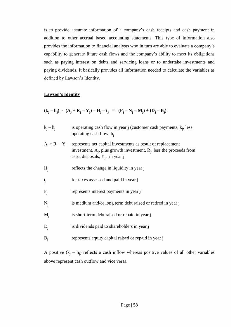
Page | 58
is to provide accurate information of a company’s cash receipts and cash payment in
addition to other accrual based accounting statements. This type of information also
provides the information to financial analysts who in turn are able to evaluate a company’s
capability to generate future cash flows and the company’s ability to meet its obligations
such as paying interest on debts and servicing loans or to undertake investments and
paying dividends. It basically provides all information needed to calculate the variables as
defined by Lawson’s Identity.
Lawson’s Identity
(kj – hj) - (Aj + Rj – Yj) – Hj – tj = (Fj – Nj – Mj) + (Dj – Bj)
kj – hj is operating cash flow in year j (customer cash payments, kj, less
operating cash flow, hj
Aj + Rj – Yj represents net capital investments as result of replacement
investment, Aj, plus growth investment, Rj, less the proceeds from
asset disposals, Yj, in year j
Hj reflects the change in liquidity in year j
tj for taxes assessed and paid in year j
Fj represents interest payments in year j
Nj is medium and/or long term debt raised or retired in year j
Mj is short-term debt raised or repaid in year j
Dj is dividends paid to shareholders in year j
Bj represents equity capital raised or repaid in year j
A positive (kj – hj) reflects a cash inflow whereas positive values of all other variables
above represent cash outflow and vice versa.
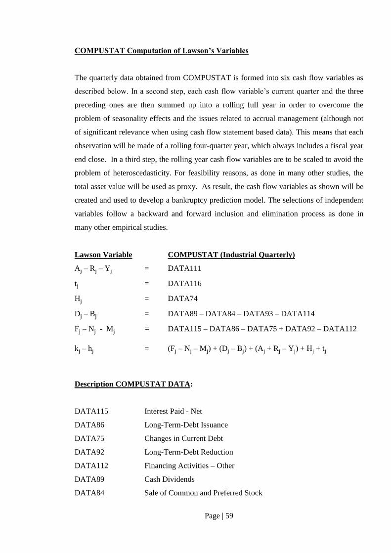
Page | 59
COMPUSTAT Computation of Lawson’s Variables
The quarterly data obtained from COMPUSTAT is formed into six cash flow variables as
described below. In a second step, each cash flow variable’s current quarter and the three
preceding ones are then summed up into a rolling full year in order to overcome the
problem of seasonality effects and the issues related to accrual management (although not
of significant relevance when using cash flow statement based data). This means that each
observation will be made of a rolling four-quarter year, which always includes a fiscal year
end close. In a third step, the rolling year cash flow variables are to be scaled to avoid the
problem of heteroscedasticity. For feasibility reasons, as done in many other studies, the
total asset value will be used as proxy. As result, the cash flow variables as shown will be
created and used to develop a bankruptcy prediction model. The selections of independent
variables follow a backward and forward inclusion and elimination process as done in
many other empirical studies.
Lawson Variable COMPUSTAT (Industrial Quarterly)
Aj – Rj – Yj = DATA111
tj = DATA116
Hj = DATA74
Dj – Bj = DATA89 – DATA84 – DATA93 – DATA114
Fj – Nj - Mj = DATA115 – DATA86 – DATA75 + DATA92 – DATA112
kj – hj = (Fj – Nj – Mj) + (Dj – Bj) + (Aj + Rj – Yj) + Hj + tj
Description COMPUSTAT DATA:
DATA115 Interest Paid - Net
DATA86 Long-Term-Debt Issuance
DATA75 Changes in Current Debt
DATA92 Long-Term-Debt Reduction
DATA112 Financing Activities – Other
DATA89 Cash Dividends
DATA84 Sale of Common and Preferred Stock
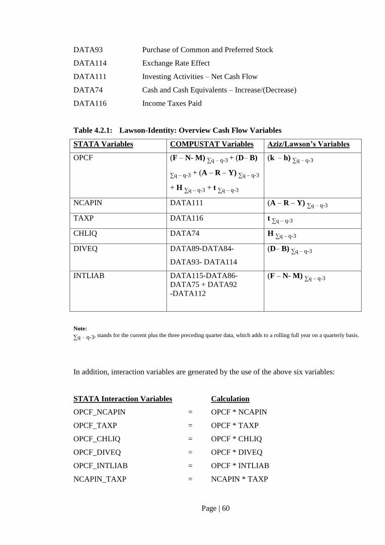
Page | 60
DATA93 Purchase of Common and Preferred Stock
DATA114 Exchange Rate Effect
DATA111 Investing Activities – Net Cash Flow
DATA74 Cash and Cash Equivalents – Increase/(Decrease)
DATA116 Income Taxes Paid
Table 4.2.1: Lawson-Identity: Overview Cash Flow Variables
STATA Variables COMPUSTAT Variables Aziz/Lawson’s Variables
OPCF (F – N- M) ∑q – q-3 + (D– B)
∑q – q-3 + (A – R – Y) ∑q – q-3
+ H ∑q – q-3 + t ∑q – q-3
(k – h) ∑q – q-3
NCAPIN DATA111 (A – R – Y) ∑q – q-3
TAXP DATA116 t ∑q – q-3
CHLIQ DATA74 H ∑q – q-3
DIVEQ DATA89-DATA84-
DATA93- DATA114
(D– B) ∑q – q-3
INTLIAB DATA115-DATA86-
DATA75 + DATA92
-DATA112
(F – N- M) ∑q – q-3
Note:
∑q – q-3, stands for the current plus the three preceding quarter data, which adds to a rolling full year on a quarterly basis.
In addition, interaction variables are generated by the use of the above six variables:
STATA Interaction Variables Calculation
OPCF_NCAPIN = OPCF * NCAPIN
OPCF_TAXP = OPCF * TAXP
OPCF_CHLIQ = OPCF * CHLIQ
OPCF_DIVEQ = OPCF * DIVEQ
OPCF_INTLIAB = OPCF * INTLIAB
NCAPIN_TAXP = NCAPIN * TAXP

Page | 61
NCAPIN_CHLIQ = NCAPIN * CHLIQ
NCAPIN_DIVEQ = NCAPIN * DIVEQ
NCAPIN_INTLIAB = NCAPIN * INTLIAB
TAXP_CHLIQ = TAXP * CHLIQ
TAXP_DIVEQ = TAXP * DIVEQ
TAXP_INTLIAB = TAXP * INTLIAB
CHLIQ_DIVEQ = CHLIQ * DIVEQ
CHLIQ_INTLIAB = CHLIQ * INTLIAB
DIVEQ_INTLIAB = DIVEQ * INTLIAB

Page | 62
Table 4.2.2: SFAS # 95: Statement of Cash Flows – Quarterly Format
STATEMENT OF CASH FLOWS
COMPUSTAT
Indirect Operating Activities
+ Income Before Extraordinary Items DATA76
+ Depreciation and Amortization DATA77
+ Extraordinary items and Discontinued Operations DATA78
+ Deferred Taxes DATA79
+ Equity in Net Loss (Earnings) DATA80
+ Sale of Property, Plant and Equipment and Sale of Investments – Loss / (Gain) DATA102
+ Funds from Operations – Other DATA81
+ Accounts Receivable – Decrease / (Increase) DATA103
+ Inventory – Decrease / (Increase) DATA104
+ Accounts Payable and Accrued Liabilities – Increase/ (Decrease) DATA105
+ Income Taxes – Accrued – Increase / (Decrease) DATA106
+ Assets and Liabilities – Other (Net Change) DATA107
= Operating Activities – Net Cash Flow DATA108
Investing Activities
- Increase in Investments DATA91
+ Sale of Investments DATA85
+ Short-Term Investments – Change DATA109
- Capital Expenditures DATA90
+ Sale of Property, Plant and Equipment DATA83
- Acquisitions DATA94
+ Investing Activities – Other DATA110
= Investing Activities – Net Cash Flow DATA111
Financing Activities
+ Sale of Common and Preferred Stock DATA84
- Purchase of Common and Preferred Stock DATA93
- Cash Dividends DATA89
+ Long-Term Debt – Issuance DATA86
- Long-Term Debt – Reduction DATA92
+ Changes in Current Debt DATA75
+ Financing Activities – Other DATA112
= Financing Activities – Net Cash Flow DATA113
+ Exchange Rate Effect DATA114
= Cash and Cash Equivalents – Increase / (Decrease)
(DATA108 + DATA111 + DATA113 + DATA114) DATA74
Add’l
Data
Income Taxes Paid DATA116
Interest Paid – Net DATA115
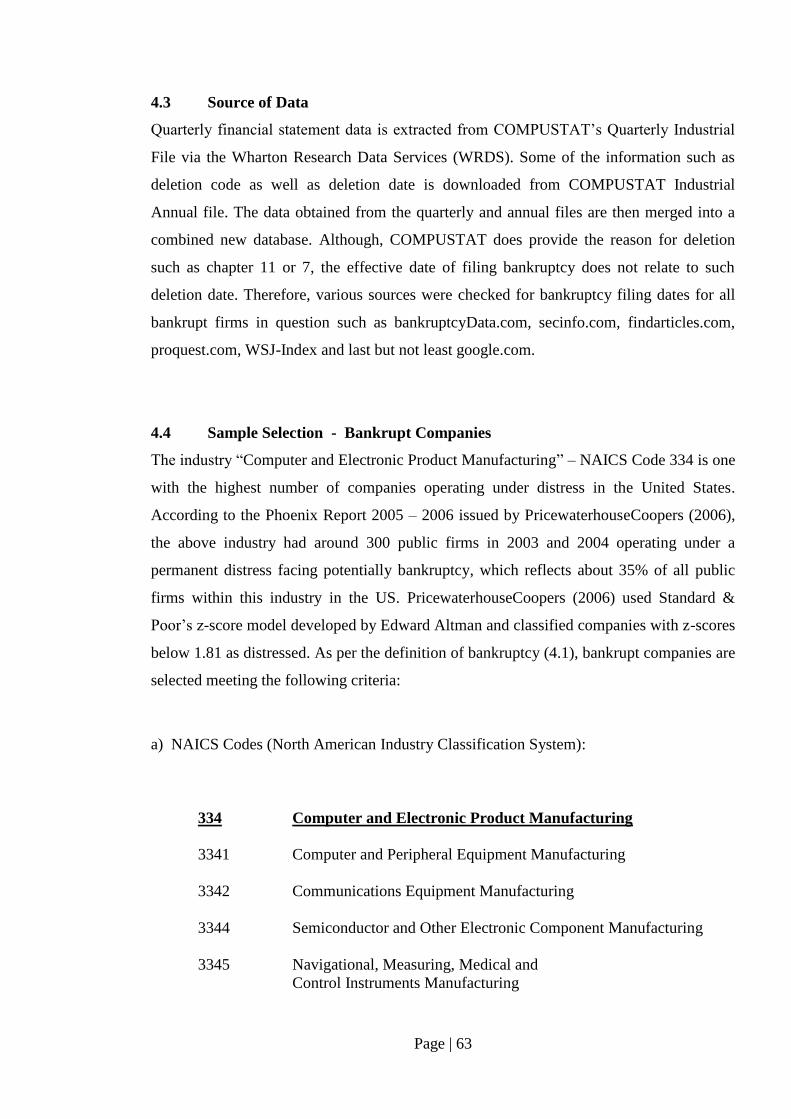
Page | 63
4.3 Source of Data
Quarterly financial statement data is extracted from COMPUSTAT’s Quarterly Industrial
File via the Wharton Research Data Services (WRDS). Some of the information such as
deletion code as well as deletion date is downloaded from COMPUSTAT Industrial
Annual file. The data obtained from the quarterly and annual files are then merged into a
combined new database. Although, COMPUSTAT does provide the reason for deletion
such as chapter 11 or 7, the effective date of filing bankruptcy does not relate to such
deletion date. Therefore, various sources were checked for bankruptcy filing dates for all
bankrupt firms in question such as bankruptcyData.com, secinfo.com, findarticles.com,
proquest.com, WSJ-Index and last but not least google.com.
4.4 Sample Selection - Bankrupt Companies
The industry “Computer and Electronic Product Manufacturing” – NAICS Code 334 is one
with the highest number of companies operating under distress in the United States.
According to the Phoenix Report 2005 – 2006 issued by PricewaterhouseCoopers (2006),
the above industry had around 300 public firms in 2003 and 2004 operating under a
permanent distress facing potentially bankruptcy, which reflects about 35% of all public
firms within this industry in the US. PricewaterhouseCoopers (2006) used Standard &
Poor’s z-score model developed by Edward Altman and classified companies with z-scores
below 1.81 as distressed. As per the definition of bankruptcy (4.1), bankrupt companies are
selected meeting the following criteria:
a) NAICS Codes (North American Industry Classification System):
334 Computer and Electronic Product Manufacturing
3341 Computer and Peripheral Equipment Manufacturing
3342 Communications Equipment Manufacturing
3344 Semiconductor and Other Electronic Component Manufacturing
3345 Navigational, Measuring, Medical and
Control Instruments Manufacturing
Page | 64
b) COMPUSTAT annual slot #35 explains the reason for deletion from the
“Industrial Annual Research File” by the footnote codes below:
01 Acquisition or merger
02 Bankruptcy – Chapter 11
03 Liquidation – Chapter 7
09 Now a private company
10 Other
The quarterly data is taken from the COMPUSTAT Industrial File. The group of
bankrupt companies consists of companies which went bankrupt under chapter 11 or
chapter 7 and which were deleted from the “Industrial Annual Research File” by code
02 and 03. In addition, several companies reported under the code 10 were deleted not
only because of voluntary delisting from stock exchange, but because of filing
bankruptcy under chapter 11 or 7. Therefore, companies filing bankruptcy, but under
footnote code 10 were also added to the group of bankrupt companies. Companies
under code 01, 09 and even companies of active status (at discretion of respective stock
exchange) may have filed for bankruptcy chapter 11, but are considered to be non-
bankrupt in the sample for modelling purpose. The assignment of these companies to
the non-bankrupt group goes under the assumption that filing for bankruptcy with
subsequent successful restructuring by merger & acquisition, going private or remaining
listed on the stock exchange does not constitute a bankruptcy resulting in full
shareholder loss as defined under point 4.1..
c) For modelling purposes all companies listed on NYSE, NASDAQ, AMEX as well as
OTCBB are included, provided that quarterly financial data has been reported as
required by the SEC (US Securities and Exchange Commission). However, OTCBB
companies will be dropped in chapter 5 where the pricing of bankruptcy risk is tested.
This exclusion is due to the issue of thin trading. Nevertheless, these companies should
not get missed for the modelling and for the purpose of validating this bankruptcy
prediction model as long as SEC compliant data is available.
Page | 65
d) As previously mentioned, cash flow reporting under SFAS No. 95 (Table 4.2.2)
became effective for firms reporting annual financial statements for fiscal years ending
after July 15, 1988. Therefore, companies’ quarterly data from the years 1988 to 2002
were included in the sample for modelling purpose.
e) The term of bankruptcy in this study follows the definition of legal act, which as
discussed (2.1.2) is very much country specific. In order to obtain an acceptable
dichotomous dependent variable, which follows the law of one national jurisdiction,
companies listed in the United States but with headquarters abroad will be dropped from
this sample (deletion of location code 99 in COMPUSTAT’s Industrial File). Foreign
(non-US) companies may have to comply with very different national laws and
procedures and as such may distort the dichotomy of the dependent variable in question.
Although, the timing difference between entering an acute state of failure and the act of
filing bankruptcy may still vary from company to company within the United States, it
is probably still the best indicator of companies facing potential liquidation and a full or
near full shareholders’ loss.
4.5 Sample Selection – Non-bankrupt Companies
The group of non-bankrupt firms is formed as follows:
a) Taken from same industries as bankrupt firms’ definition under 4.4 a)
b) Companies which have not been deleted from the COMPUSTAT Industrial File in the
years before 1988 until 2006, which also includes the 4-year-period after the 15 year
window are considered to be non-bankrupt. This means that companies that may have
filed for Chapter 11, but either
i) remained listed at discretion of the board of stock exchange, which
were not deleted on the COMPUSTAT Industrial File and finally
survived as per end of 2006 or
ii) “survived” as merger & acquisition candidate and finally have been
deleted with code “01 Acquisition or merger” (COMPUSTAT annual
slot #35) or
iii) Went private under code “09 Now a private company”
(COMPUSTAT annual slot #35)

Page | 66
are considered to be non-bankrupt companies. None of these companies’ deletion on the
COMPUSTAT Industrial File has been coded either “02 Bankruptcy – Chapter 11” or
“03 Liquidation – Chapter 7”, but with the codes as mentioned above. As per definition
of bankruptcy and the related dichotomous variable, it is also justified to classify these
companies as non-bankrupt since they survived in one way or the other until 2006 (after
the sample period) and as such most likely have not resulted in a nearly full or full
shareholders’ loss. Also, the information for delisted companies other than bankruptcy
are restricted and in most of the cases not accessible. Hence, any classification attempt
for these companies may be subjective as the economic and legal outcome or
development is unknown. As result, companies as described under ii) to iii) have been
exiting the spell (code 0), but not as failure companies (code 1).
c) All other criteria for inclusion or exclusion of non-bankrupt companies are the same as
described for the bankrupt ones above in section 4.4.
As per section 2.1.4.3, the sample should represent the population of all firms. Therefore, I
will not use the quite often chosen method of matched pair (50 per cent of each group
matched by asset size and industry etc). This would simply result in oversampling of
bankrupt firms. Although, Aziz, Emanuel and Lawson (1988) state that an oversampling
does benefit the overproportionally high cost of predicting a bankrupt firm. I argue that the
cost of prediction is not of relevance for this study to be conducted, it is rather a question
of feasibility. In addition, I also plan to measure the relationship between an industry
specific portfolio’s stock returns and the risk of failure proxied by this bankruptcy
prediction model. Therefore, I will only choose one industry and construct a sample
specific model in order to make this study feasible for the stated reasons below. All data,
both accounting and market data will be drawn from and empirically tested for one specific
industry only, but validated with out-of-sample tests (section 4.8) covering the period 2003
to 2006. For the within- and out-of-sample tests I will limit my work to the industry as
defined in section 4.4 for the following reasons:
1. I do not expect to gain any additional knowledge by testing the market as a whole,
which would be an enormous amount of data to be dealt with
Page | 67
2. Some studies found that bankruptcy predictors may vary from industry to industry.
Therefore, I would have to include either additional dummies for specific industries
when modelling or simply construct one industry specific model. The latter has
been chosen for feasibility reasons and believing that a highly predictive model
based on sufficient amount of data can be obtained and be used for relationship
testing with equity returns.
4.6 Hazard Model – Cox Proportional Regression Modelling
The data set for bankrupt companies will include quarterly data which is formed into
quarterly rolling years. This means that for each company’s rolling quarter year there is
one observation which includes the information such as ticker name, the cash flow
variables as outlined under 4.2.1, the number of period of an observation (used as
equivalent to trading age) as well as a binary variable indicating whether the firm has left
the spell due to bankruptcy (Code = 1) or because of other reasons like merger &
acquisition, delisting, going private or simply because the observations stopped with the 4th
quarter in 2002. Unless it is the last observation prior filing bankruptcy, observations are
coded with “0”. For example, when a bankrupt company has reported 10 quarters of
financial statement data prior bankruptcy filing, the 10th
observation being the one prior
bankruptcy is coded with “1” and all previous quarter observations are coded “0”. For non-
bankrupt companies all observations up to 60 quarter data (1988 to 2002) are coded “0”
regardless when and why they have left the spell during the observation period. All values
being lower than the 1st percentile or higher than the 99
th percentile, will be replaced with
the 1st or 99
th percentile in order to remove outliers (section 2.1.3.4). Missing values (very
few cases) are replaced by the prior quarter data. This is considered to be conservative
since the model will have to deal with data which is more distant to the date of event.
A model with the highest predictive power will be obtained by the test of variables (section
4.2) using a Cox Proportional Hazard model. The stepwise approach is followed to select
significant covariates and interactions, but also manually obtained combinations of
covariates are examined. The variables selected are then tested for multicollinearity
(section 4.7.2). The bankruptcy prediction model will be run for each bankrupt company
and for each of the 12 quarters prior the unfortunate event in order to obtain an accuracy of
classification matrix.
Page | 68
4.7 Robustness Checks
As with any other model such as ordinary least squares, there are also some checks to be
done with the model obtained by the Cox regression. These checks include the testing of
the proportional hazards assumption as suggested by Cleves, Gould and Gutierrez (2003)
as well as some tests related to multicollinearity, a problem very often found in studies
using accounting ratios.
4.7.1 Testing the Proportional Hazards Assumption
The tests based on re-estimation as well as based on Schoenfeld residuals are to be
performed in order to obtain certainty that the model has been adequately parameterized
and that a good specification for xx has been selected.
The first test based on re-estimation is called a “linktest”, which is a STATA function and
translates into the following equation (Cleves, Gould and Gutierrez 2003):
+
The linktest above provides the certainty that the coefficient on the squared linear predictor
is significant and that if the hazard model is properly specified, one should not be able to
find additional independent variables that are significant. First, x needs to be estimated
from the standard Cox model and than 1 and 2 from a second round model. If we expect
xx to be the correct model specification, 1 has to equal 1 and 2 has to equal 0. In order
to facilitate this above test, the linktest creates two new variables called _hat and _hatsq,
which then gets refitted using these two variables as predictors. If the model is correctly
specified one should expect variable _hat to be significant since it is the predicted value
. The second variable _hatsq is expected to be insignificant because
the squared predictions should not result in much explanatory power. Therefore, _hat
should yield in a p-value lower or equal 0.05 and _hatsq should as result of insignificance
have a p-value higher than 0.05. If the model detects the presence of omitted variables by
_hatsq being significant, a partially new model needs to be reconfigured again. This test is
performed under 4.9.3.1.
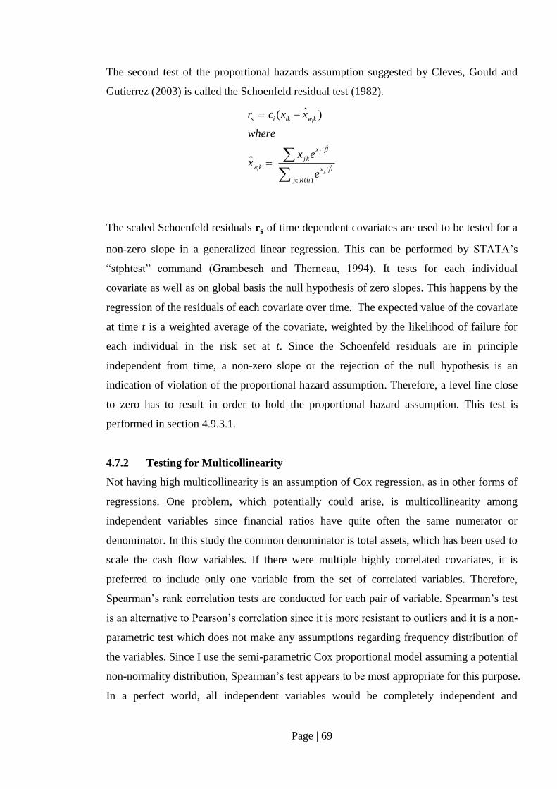
Page | 69
The second test of the proportional hazards assumption suggested by Cleves, Gould and
Gutierrez (2003) is called the Schoenfeld residual test (1982).
The scaled Schoenfeld residuals rs of time dependent covariates are used to be tested for a
non-zero slope in a generalized linear regression. This can be performed by STATA’s
“stphtest” command (Grambesch and Therneau, 1994). It tests for each individual
covariate as well as on global basis the null hypothesis of zero slopes. This happens by the
regression of the residuals of each covariate over time. The expected value of the covariate
at time t is a weighted average of the covariate, weighted by the likelihood of failure for
each individual in the risk set at t. Since the Schoenfeld residuals are in principle
independent from time, a non-zero slope or the rejection of the null hypothesis is an
indication of violation of the proportional hazard assumption. Therefore, a level line close
to zero has to result in order to hold the proportional hazard assumption. This test is
performed in section 4.9.3.1.
4.7.2 Testing for Multicollinearity
Not having high multicollinearity is an assumption of Cox regression, as in other forms of
regressions. One problem, which potentially could arise, is multicollinearity among
independent variables since financial ratios have quite often the same numerator or
denominator. In this study the common denominator is total assets, which has been used to
scale the cash flow variables. If there were multiple highly correlated covariates, it is
preferred to include only one variable from the set of correlated variables. Therefore,
Spearman’s rank correlation tests are conducted for each pair of variable. Spearman’s test
is an alternative to Pearson’s correlation since it is more resistant to outliers and it is a non-
parametric test which does not make any assumptions regarding frequency distribution of
the variables. Since I use the semi-parametric Cox proportional model assuming a potential
non-normality distribution, Spearman’s test appears to be most appropriate for this purpose.
In a perfect world, all independent variables would be completely independent and
ˆ'
ˆ'
( )
ˆ( )
ˆ
i
j
i j
s i ik w k
x
j k
w k x
j R ti
r c x x
where
x ex
e
Page | 70
unrelated to each other, but reality shows though that virtually every multiple regression
has some collinearity between the independent covariates. There are no clear-cut rules
about the level of collinearity to be excluded from a model, but if it exceeds 0.75 it would
probably make sense to drop one of the highly correlated variables and to rework the
model specification again. This test is performed in section 4.9.3.2.
4.8 External Validation by Hold-Out Sample and Benchmark
In addition to the robustness checks as described in section 4.7, it is well documented that
empirically derived bankruptcy models very often lose their predictive power or
forecasting ability when applied ex ante (Grice and Ingram 2001; Begley, Ming and Watts
1996). One method for the model validation is the use of a hold-out sample. The idea is
that the model obtained from the primary data set covering the years 1988 to 2002 will be
run thru a new unrelated data set and tested for its accuracy rates of bankruptcy prediction
classifications (section 4.8.1). In addition, the result of the hold-out sample will be
benchmarked with Altman’s Z-Score model by using a Receiver Operating Characteristics
curve as discussed under section 4.8.2 below.
4.8.1 Hold-Out Sample
The selection of bankrupt and non-bankrupt companies follows the same procedures as
described in sections 4.3 to 4.5. Also, the sample includes the companies from the same
industries as outlined in section 4.4 and covers the period 2003 - 2006. The classification
results are to be compared to the model sample (1988 to 2002) for both categories, the
bankrupt and the non-bankrupt firms.
4.8.2 Receiver Operating Characteristic (ROC) Benchmark with Z-Score
The Receiver Operating Characteristics (ROC) curve, as discussed in all details by
Sobehart et al. (2000), is a widely accepted method to measure the overall prediction
accuracy across multiple models (Chava and Jarrow (2004); Agarwal and Taffler, 2008).
The benchmark with Altman’s Z-Score Model, as briefly discussed further below, is based
on the application of the ROC model by using the hold-out sample for the years 2003 to
2006. This allows comparing both models with data not being used for modelling purposes.
Following Agarwal and Taffler (2008), the areas under the curve are estimated by the use
of the Wilcoxon statistic (Hanley and McNeil, 1982) and evaluated by the Hanley and
Page | 71
McNeil (1983) test statistics that adjust for the correlation resulting from the application of
the two models on the same sample. The ROC curves are constructed by ranking a model’s
risk of failure from high to low and are linked with a firm’s effective status of failure or
non-failure for each quarter in the period from 2003 to 2006. The model measures to what
extent firms failed are actually found within the first percentage of firms being predicted
high risk failure candidates. This analysis (result see figure 4.9.4) will provide both the
area under the curve (AUC) and, as a simple linear transformation (Engelmann et al., 2003;
see below), the accuracy ratio (AR) for each of the models tested.
Accuracy Ratio = 2 * (area under ROC curve – 0.50)
An AUC value of 0.5 which is an AR of 0.00 is considered to be a random model which
has no predictive ability. A perfect model would result in an AUC value of 1.0
corresponding to an AR of 1.00. The results of this benchmark are discussed under section
4.9.6 and depicted in figure 4.9.4.
The benchmark model as previously mentioned is the Z-Score model (Altman, 1968). This
model derived from an MDA analysis as described in section 2.1.3.2 still enjoys popularity
in the industry and is shown below:
Z = 1.2X1 + 1.4X2 + 3.3X3 + 0.6X4 + 1.0X5
where:
X1 = working capital/total assets
X2 = retained earnings/total assets
X3 = earnings before interest and taxes/total assets
X4 = market value equity/book value of total liabilities
X5 = sales/total assets
Z = overall index
The first difference between the cash flow based prediction model of this study and the Z-
Score is obviously given by the fact the Altman’s variables above are accrual based
Page | 72
accounting ratios with the exception of market value equity. In this study cash flow based
accounting variables are used only. The second difference is that the Z-Score model has
not been developed using panel data company information, but it has been constructed
using cross-section data only. Other differences of the Z-Score compared to the cash flow
based prediction model is provided by the facts that a) it is a multiple non-industry specific
model which primarily includes manufacturing firms, b) it has been based on a matched
pair sample selection process of an initial 66 firms consisting of 33 healthy and 33
bankrupt firms only. As result, the Z-Score relies on much fewer observations than this
study’s cash flow derived model which is expected to be built on more than 1,000 firms
consisting of almost 40,000 firm quarter observations. Although, it is not the ultimate goal
to achieve better results by the use of this new cash flow based bankruptcy prediction
model, it is of importance to obtain validation by the ROC benchmark and to provide
probabilities of going bankrupt as well as cash flow coefficients for either type of
companies. Overall, I expect to obtain a highly predictive model with an accuracy ratio of
at least the same level as achieved by Altman’s Z-Score, which can be used for the tests to
be conducted as described in chapter 5. Both data sets, within- and out-of-sample are
expected to provide the probabilities of failure as well as related cash flow coefficients
which can be used for asset pricing and portfolio testing as outlined in section 5.1.
4.8.3 Distress Risk a Continuous Probability of Default Measure
As previously mentioned, the probabilities of bankruptcy risk derived from the cash flow
based bankruptcy prediction model are used as a proxy for the asset pricing tests related to
distress risk. Although, the predictive power of such model may be superior in an out-of-
sample benchmark test, it still needs to be tested for its measure characteristic to see if it is
a continuous or binary default risk measure. Depending on its outcome, the distress risk
factor to be used for subsequent assets pricing tests would be either the probabilities of
going bankrupt when continuous or simply binary with 0 or 1.
In section 4.9.7, the distress risk measure is tested by tabulating the probability of default
deciles against the failure rates to evaluate first, if it is a continuous measure and second if
there is an appropriate degree of association.
Page | 73
4.9 Results
4.9.1 Results on Selection and Data Obtained (Descriptive)
Following the selection process as outlined in sections 4.4 and 4.5, the summary statistics
is reported as shown in Table 4.9.1.1. The statistics is limited to the four variables of the
model obtained in section 4.9.2. The dataset consists of 39’164 quarterly calculated full
years on quarterly rolling basis. This total number of observations stems from 1’183 firms.
2’309 observations are derived from 82 bankrupt firms as per Table 4.9.1.2 and another
36’855 observations from 1’101 non-bankrupt firms. The top 50 companies of the non-
bankrupt firms are listed in Table 4.9.1.3 and the smallest 50 non-bankrupt ones are shown
in Table 4.9.1.4. The summary statistics (table 4.9.1.1) reveals expected differences
between the two groups. The overall operating cash flow variable (OPCF) which is scaled
by total assets shows that the mean of all firm observations is negative 0.007. This means
that this industry produces on average negative cash flows from operating activities. This is
not surprising, since the PricewaterhouseCoopers study (2006) has indicated that more than
35% do operate in a near bankruptcy mode. I will not go into further discussion why under
normal circumstances negative cash flows from operating activities may result in
bankruptcy one day. Also, the scaled OPCF mean of -0.162 for the bankrupt group reflects
higher cash drains compared to positive 0.003 for non-bankrupt companies, which supports
the fact that positive cash flows from operating activities are vital. The next variable TAXP
which reflects the cash flow component “tax paid” does also meet expectations, at least
from an intuitive point of view. A negative TAXP in this study means that taxes were paid,
which is normally the case when profits were produced as well as in most cases cash was
generated and where potential losses from previous periods did not offset all taxes due
from the current reporting period. Therefore, the mean of TAXP with -0.018 for the non-
bankrupt group is more negative than the one for the bankrupt group. The third variable
INTLIAB basically reflects the cash flow from debt financing activities including interest
being paid. The mean of INTLIAB with -0.001 for non-bankrupt firms is less negative
than the one for bankrupt firms with a mean of -0.017. The interpretation of negative mean
for this variable is that there is a net cash outflow from long-term debt retirement over debt
financing. Bankrupt companies may be forced to repay their debts at faster rate their non-
bankrupt counterparts, which in turn may leverage their company given their healthy status

Page | 74
even further. Debt financing may secure the company’s financial position to a certain
extent but it appears that it is more difficult to obtain for bankruptcy candidates, which in
turn may lead to liquidity issues. Overall, the ability to repay debt and pay interests is
considered to be obviously a stronger factor of survivability than increasing a company’s
debt position. The last interaction variable OPCF_TAXP is the product of OPCF and
TAXP. The interaction term shows a conditionality between operating cash flow and taxes
paid. This is obvious since a unit increase / (decrease) in operating cash flows (assuming
the same impact on taxable profits) will increase / (decrease) the taxes to be paid
accordingly.
Table 4.9.1.1 : Summary Statistics
Table 4.9.1.2 shows the list of 82 bankrupt companies. It clearly demonstrates that
companies of all kind of size measured by total assets prior bankruptcy have filed for
bankruptcy and therefore are included in this sample. The largest three in the years 1988 to
Variable Obs Mean Std. Dev.
OPCF 39'164 -0.007 0.632
INTLIAB 39'164 -0.002 0.159
TAXP 39'164 -0.017 0.028
OPCF_TAXP 39'164 -0.003 0.007
Bankrupt Firms
Variable Obs Mean Std. Dev.
OPCF 2'309 -0.162 0.493
INTLIAB 2'309 -0.017 0.222
TAXP 2'309 -0.006 0.020
OPCF_TAXP 2'309 -0.001 0.005
Non-Bankrupt Firms
Variable Obs Mean Std. Dev.
OPCF 36'855 0.003 0.638
INTLIAB 36'855 -0.001 0.154
TAXP 36'855 -0.018 0.028
OPCF_TAXP 36'855 -0.003 0.007
Page | 75
2002 were Memorex Telex with assets exceeding $ 1bn, Commodore International with
total assets of $ 266m or Everex Systems with $ 255m prior filing bankruptcy. Obviously
the value of assets was significantly higher in the years prior failure. The smallest bankrupt
firms measured by total assets prior bankruptcy filing were Solopoint with $ 212k, Zonic
with $ 625k or Scientific Measurement System with $ 642k. The list also reveals that the
majority of companies were delisted as result of filing bankruptcy under Chapter 11 and
only a few went straight into liquidation thru Chapter 7.
For the non-bankrupt firms table 4.9.1.3 shows the largest 50 companies of this industry as
per Q1 in 2000 consisting of reputable firms such as Intel Corp. with total assets of $ 48bn,
Motorola Inc with $ 43bn, Hewlett Packard Corp with $ 34bn, Xerox Corp with $30bn or
Compaq (before merger with HP) with $28bn to name a few. However, also in this group,
small companies were included in the sample for modelling purpose. Table 4.9.1.4 shows
the 50 smallest non-bankrupt firms of this industry as per Q1 in 2000 with total assets in
the range of $ 1 to 4m only.
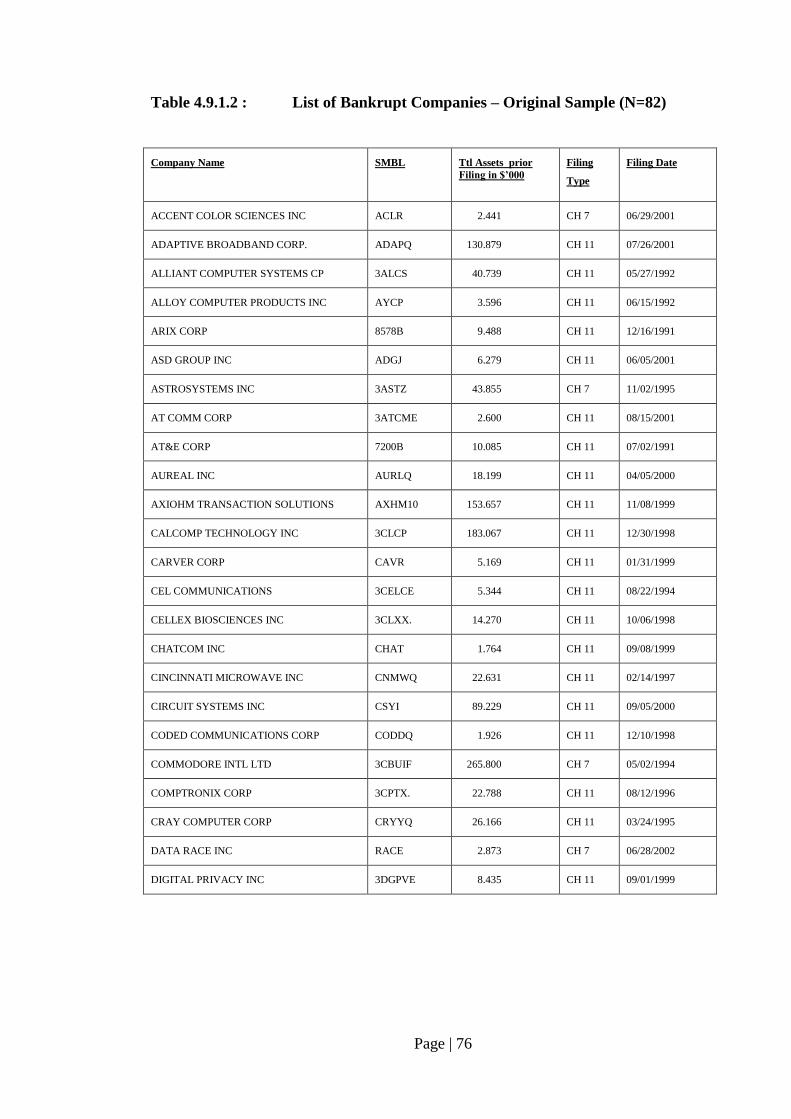
Page | 76
Table 4.9.1.2 : List of Bankrupt Companies – Original Sample (N=82)
Company Name SMBL Ttl Assets prior
Filing in $’000
Filing
Type
Filing Date
ACCENT COLOR SCIENCES INC ACLR 2.441 CH 7 06/29/2001
ADAPTIVE BROADBAND CORP. ADAPQ 130.879 CH 11 07/26/2001
ALLIANT COMPUTER SYSTEMS CP 3ALCS 40.739 CH 11 05/27/1992
ALLOY COMPUTER PRODUCTS INC AYCP 3.596 CH 11 06/15/1992
ARIX CORP 8578B 9.488 CH 11 12/16/1991
ASD GROUP INC ADGJ 6.279 CH 11 06/05/2001
ASTROSYSTEMS INC 3ASTZ 43.855 CH 7 11/02/1995
AT COMM CORP 3ATCME 2.600 CH 11 08/15/2001
AT&E CORP 7200B 10.085 CH 11 07/02/1991
AUREAL INC AURLQ 18.199 CH 11 04/05/2000
AXIOHM TRANSACTION SOLUTIONS AXHM10 153.657 CH 11 11/08/1999
CALCOMP TECHNOLOGY INC 3CLCP 183.067 CH 11 12/30/1998
CARVER CORP CAVR 5.169 CH 11 01/31/1999
CEL COMMUNICATIONS 3CELCE 5.344 CH 11 08/22/1994
CELLEX BIOSCIENCES INC 3CLXX. 14.270 CH 11 10/06/1998
CHATCOM INC CHAT 1.764 CH 11 09/08/1999
CINCINNATI MICROWAVE INC CNMWQ 22.631 CH 11 02/14/1997
CIRCUIT SYSTEMS INC CSYI 89.229 CH 11 09/05/2000
CODED COMMUNICATIONS CORP CODDQ 1.926 CH 11 12/10/1998
COMMODORE INTL LTD 3CBUIF 265.800 CH 7 05/02/1994
COMPTRONIX CORP 3CPTX. 22.788 CH 11 08/12/1996
CRAY COMPUTER CORP CRYYQ 26.166 CH 11 03/24/1995
DATA RACE INC RACE 2.873 CH 7 06/28/2002
DIGITAL PRIVACY INC 3DGPVE 8.435 CH 11 09/01/1999
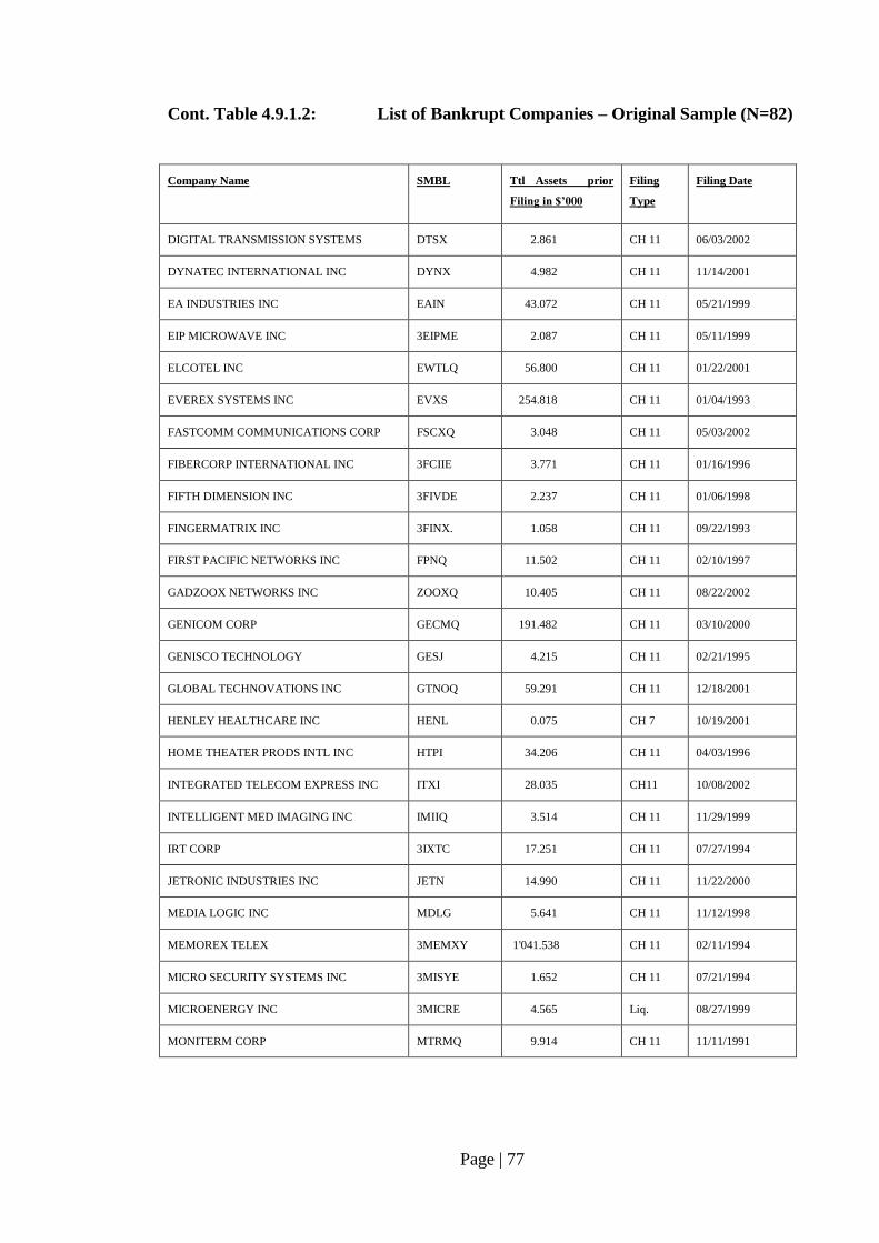
Page | 77
Cont. Table 4.9.1.2: List of Bankrupt Companies – Original Sample (N=82)
Company Name SMBL Ttl Assets prior
Filing in $’000
Filing
Type
Filing Date
DIGITAL TRANSMISSION SYSTEMS DTSX 2.861 CH 11 06/03/2002
DYNATEC INTERNATIONAL INC DYNX 4.982 CH 11 11/14/2001
EA INDUSTRIES INC EAIN 43.072 CH 11 05/21/1999
EIP MICROWAVE INC 3EIPME 2.087 CH 11 05/11/1999
ELCOTEL INC EWTLQ 56.800 CH 11 01/22/2001
EVEREX SYSTEMS INC EVXS 254.818 CH 11 01/04/1993
FASTCOMM COMMUNICATIONS CORP FSCXQ 3.048 CH 11 05/03/2002
FIBERCORP INTERNATIONAL INC 3FCIIE 3.771 CH 11 01/16/1996
FIFTH DIMENSION INC 3FIVDE 2.237 CH 11 01/06/1998
FINGERMATRIX INC 3FINX. 1.058 CH 11 09/22/1993
FIRST PACIFIC NETWORKS INC FPNQ 11.502 CH 11 02/10/1997
GADZOOX NETWORKS INC ZOOXQ 10.405 CH 11 08/22/2002
GENICOM CORP GECMQ 191.482 CH 11 03/10/2000
GENISCO TECHNOLOGY GESJ 4.215 CH 11 02/21/1995
GLOBAL TECHNOVATIONS INC GTNOQ 59.291 CH 11 12/18/2001
HENLEY HEALTHCARE INC HENL 0.075 CH 7 10/19/2001
HOME THEATER PRODS INTL INC HTPI 34.206 CH 11 04/03/1996
INTEGRATED TELECOM EXPRESS INC ITXI 28.035 CH11 10/08/2002
INTELLIGENT MED IMAGING INC IMIIQ 3.514 CH 11 11/29/1999
IRT CORP 3IXTC 17.251 CH 11 07/27/1994
JETRONIC INDUSTRIES INC JETN 14.990 CH 11 11/22/2000
MEDIA LOGIC INC MDLG 5.641 CH 11 11/12/1998
MEMOREX TELEX 3MEMXY 1'041.538 CH 11 02/11/1994
MICRO SECURITY SYSTEMS INC 3MISYE 1.652 CH 11 07/21/1994
MICROENERGY INC 3MICRE 4.565 Liq. 08/27/1999
MONITERM CORP MTRMQ 9.914 CH 11 11/11/1991
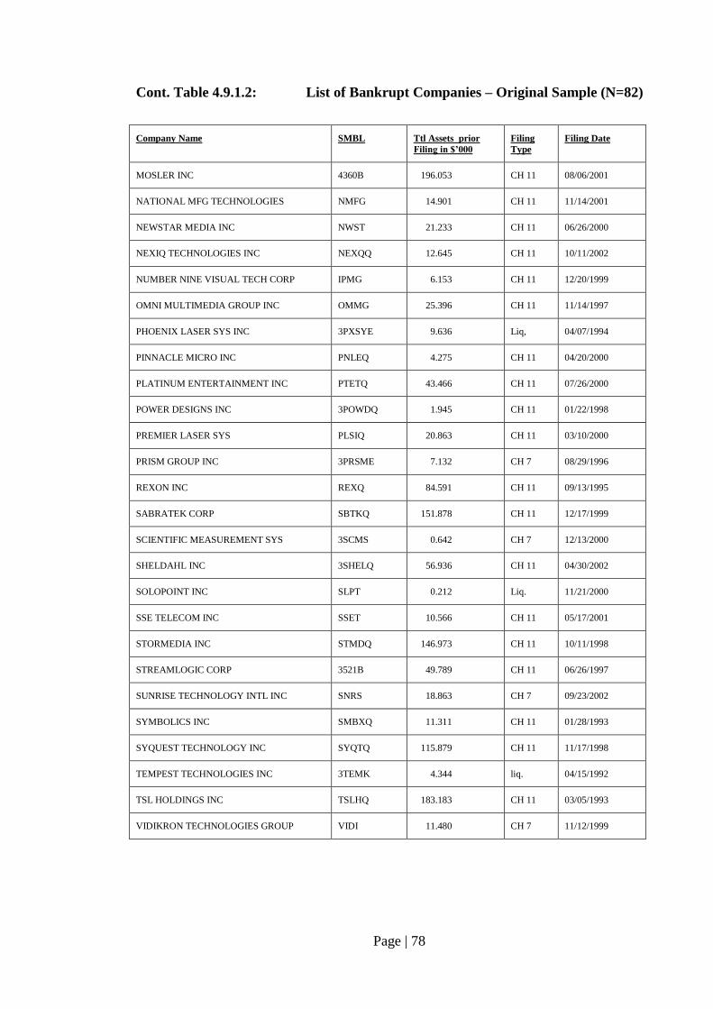
Page | 78
Cont. Table 4.9.1.2: List of Bankrupt Companies – Original Sample (N=82)
Company Name SMBL Ttl Assets prior
Filing in $’000
Filing
Type
Filing Date
MOSLER INC 4360B 196.053 CH 11 08/06/2001
NATIONAL MFG TECHNOLOGIES NMFG 14.901 CH 11 11/14/2001
NEWSTAR MEDIA INC NWST 21.233 CH 11 06/26/2000
NEXIQ TECHNOLOGIES INC NEXQQ 12.645 CH 11 10/11/2002
NUMBER NINE VISUAL TECH CORP IPMG 6.153 CH 11 12/20/1999
OMNI MULTIMEDIA GROUP INC OMMG 25.396 CH 11 11/14/1997
PHOENIX LASER SYS INC 3PXSYE 9.636 Liq, 04/07/1994
PINNACLE MICRO INC PNLEQ 4.275 CH 11 04/20/2000
PLATINUM ENTERTAINMENT INC PTETQ 43.466 CH 11 07/26/2000
POWER DESIGNS INC 3POWDQ 1.945 CH 11 01/22/1998
PREMIER LASER SYS PLSIQ 20.863 CH 11 03/10/2000
PRISM GROUP INC 3PRSME 7.132 CH 7 08/29/1996
REXON INC REXQ 84.591 CH 11 09/13/1995
SABRATEK CORP SBTKQ 151.878 CH 11 12/17/1999
SCIENTIFIC MEASUREMENT SYS 3SCMS 0.642 CH 7 12/13/2000
SHELDAHL INC 3SHELQ 56.936 CH 11 04/30/2002
SOLOPOINT INC SLPT 0.212 Liq. 11/21/2000
SSE TELECOM INC SSET 10.566 CH 11 05/17/2001
STORMEDIA INC STMDQ 146.973 CH 11 10/11/1998
STREAMLOGIC CORP 3521B 49.789 CH 11 06/26/1997
SUNRISE TECHNOLOGY INTL INC SNRS 18.863 CH 7 09/23/2002
SYMBOLICS INC SMBXQ 11.311 CH 11 01/28/1993
SYQUEST TECHNOLOGY INC SYQTQ 115.879 CH 11 11/17/1998
TEMPEST TECHNOLOGIES INC 3TEMK 4.344 liq. 04/15/1992
TSL HOLDINGS INC TSLHQ 183.183 CH 11 03/05/1993
VIDIKRON TECHNOLOGIES GROUP VIDI 11.480 CH 7 11/12/1999
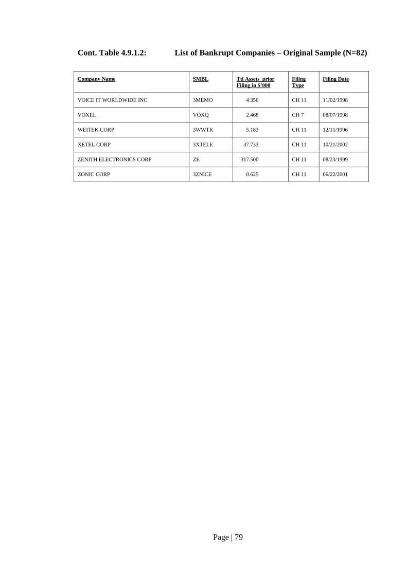
Page | 79
Cont. Table 4.9.1.2: List of Bankrupt Companies – Original Sample (N=82)
Company Name SMBL Ttl Assets prior
Filing in $’000
Filing
Type
Filing Date
VOICE IT WORLDWIDE INC 3MEMO 4.356 CH 11 11/02/1998
VOXEL VOXQ 2.468 CH 7 08/07/1998
WEITEK CORP 3WWTK 5.183 CH 11 12/11/1996
XETEL CORP 3XTELE 37.733 CH 11 10/21/2002
ZENITH ELECTRONICS CORP ZE 317.500 CH 11 08/23/1999
ZONIC CORP 3ZNICE 0.625 CH 11 06/22/2001
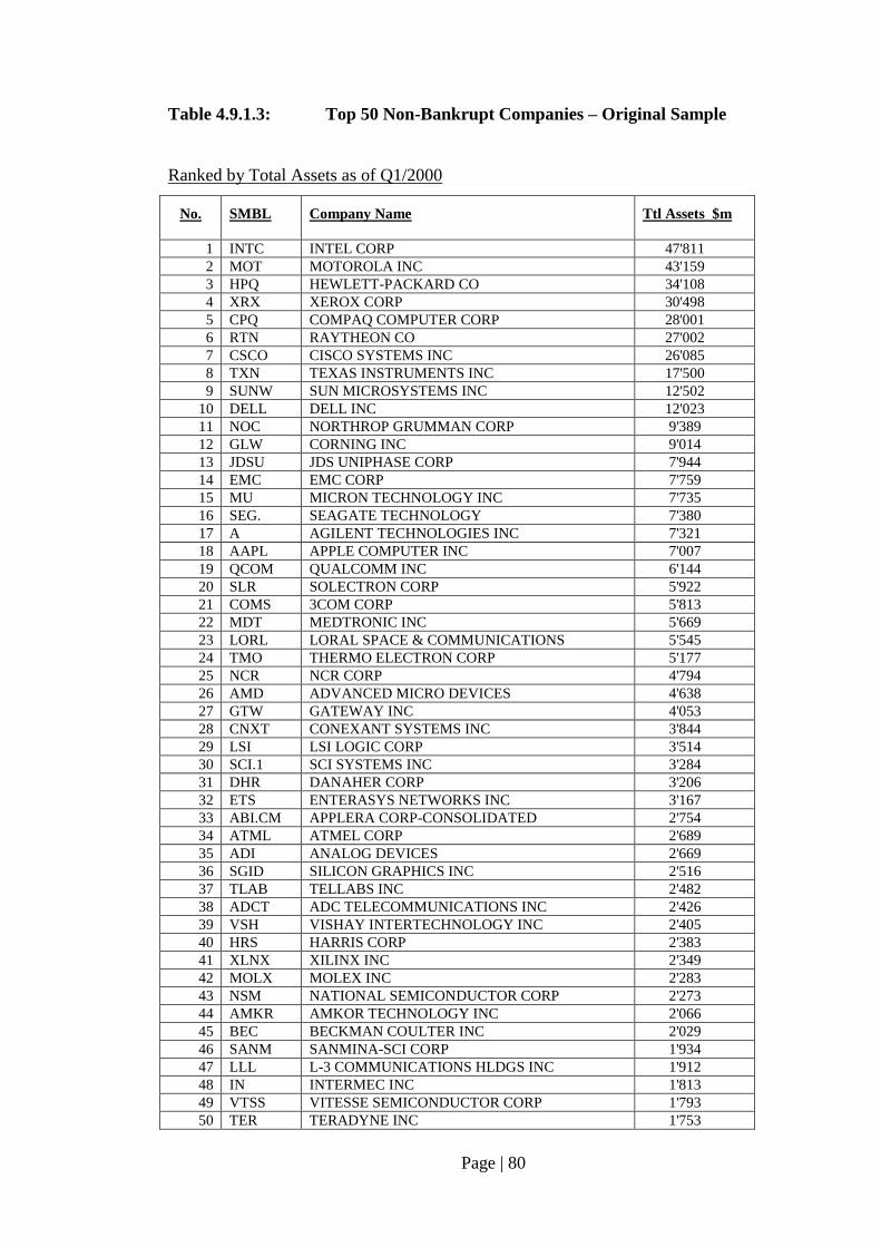
Page | 80
Table 4.9.1.3: Top 50 Non-Bankrupt Companies – Original Sample
Ranked by Total Assets as of Q1/2000
No. SMBL Company Name Ttl Assets $m
1 INTC INTEL CORP 47'811
2 MOT MOTOROLA INC 43'159
3 HPQ HEWLETT-PACKARD CO 34'108
4 XRX XEROX CORP 30'498
5 CPQ COMPAQ COMPUTER CORP 28'001
6 RTN RAYTHEON CO 27'002
7 CSCO CISCO SYSTEMS INC 26'085
8 TXN TEXAS INSTRUMENTS INC 17'500
9 SUNW SUN MICROSYSTEMS INC 12'502
10 DELL DELL INC 12'023
11 NOC NORTHROP GRUMMAN CORP 9'389
12 GLW CORNING INC 9'014
13 JDSU JDS UNIPHASE CORP 7'944
14 EMC EMC CORP 7'759
15 MU MICRON TECHNOLOGY INC 7'735
16 SEG. SEAGATE TECHNOLOGY 7'380
17 A AGILENT TECHNOLOGIES INC 7'321
18 AAPL APPLE COMPUTER INC 7'007
19 QCOM QUALCOMM INC 6'144
20 SLR SOLECTRON CORP 5'922
21 COMS 3COM CORP 5'813
22 MDT MEDTRONIC INC 5'669
23 LORL LORAL SPACE & COMMUNICATIONS 5'545
24 TMO THERMO ELECTRON CORP 5'177
25 NCR NCR CORP 4'794
26 AMD ADVANCED MICRO DEVICES 4'638
27 GTW GATEWAY INC 4'053
28 CNXT CONEXANT SYSTEMS INC 3'844
29 LSI LSI LOGIC CORP 3'514
30 SCI.1 SCI SYSTEMS INC 3'284
31 DHR DANAHER CORP 3'206
32 ETS ENTERASYS NETWORKS INC 3'167
33 ABI.CM APPLERA CORP-CONSOLIDATED 2'754
34 ATML ATMEL CORP 2'689
35 ADI ANALOG DEVICES 2'669
36 SGID SILICON GRAPHICS INC 2'516
37 TLAB TELLABS INC 2'482
38 ADCT ADC TELECOMMUNICATIONS INC 2'426
39 VSH VISHAY INTERTECHNOLOGY INC 2'405
40 HRS HARRIS CORP 2'383
41 XLNX XILINX INC 2'349
42 MOLX MOLEX INC 2'283
43 NSM NATIONAL SEMICONDUCTOR CORP 2'273
44 AMKR AMKOR TECHNOLOGY INC 2'066
45 BEC BECKMAN COULTER INC 2'029
46 SANM SANMINA-SCI CORP 1'934
47 LLL L-3 COMMUNICATIONS HLDGS INC 1'912
48 IN INTERMEC INC 1'813
49 VTSS VITESSE SEMICONDUCTOR CORP 1'793
50 TER TERADYNE INC 1'753

Page | 81
Table 4.9.1.4: Smallest 50 Non-Bankrupt Companies – Original Sample
Ranked by Total Assets as of Q1/2000
No. SMBL Company Name Ttl Assets $m
1 3HSYN HOMELAND SECURITY NETWRK INC 1
2 MGTC MEGATECH CORP 1
3 CDOC PANDA PROJECT INC 1
4 3DYTM DYNATEM INC 1
5 NVEC NVE CORP 1
6 3DIAC DIAPULSE CORP OF AMERICA 1
7 3IAUS INTL AUTOMATED SYSTEMS INC 1
8 3MMTC MICRO IMAGING TECHNOLOGY INC 1
9 3ISEC ISECURETRAC CORP 1
10 TTLO TOROTEL INC 2
11 CLSI CLANCY SYSTEMS INTL INC 2
12 DION DIONICS INC 2
13 3CRLI CIRCUIT RESEARCH LABS INC 2
14 SPHG SP HOLDING CORP 2
15 3SPHG SP HOLDING CORP 2
16 VRTC VERITEC INC 2
17 3MDTA MEGADATA CORP 2
18 3DLNKQ DECISIONLINK INC 2
19 3CBEX CAMBEX CORP 2
20 3VSNI VISEON INC 2
21 3PKPT PACKETPORT.COM INC 2
22 3BLFS BIOLIFE SOLUTIONS INC 2
23 3DYXC DIASYS CORP 2
24 3ADOT ADVANCED OPTICS ELECTRONICS 2
25 3ELST ELECTRONIC SYSTEM TECH INC 2
26 BSM BSD MEDICAL CORP/DE 2
27 TLDT TELIDENT INC 3
28 3CYBD CYBER DIGITAL INC 3
29 PMDL PACE MEDICAL INC 3
30 DLFG DIGITAL LIFESTYLES GROUP INC 3
31 LGMTA LOGIMETRICS INC 3
32 CRII CELL ROBOTICS INTL INC 3
33 ISWI INTERACTIVE SYSTEMS WORLDWDE 3
34 3IGTI IMAGE GUIDED TECHNLGIES INC 3
35 3WTRO WI-TRON INC 3
36 3IEHC IEH CORP 3
37 3SNSGE SENSE TECHNOLOGIES INC 3
38 CYDI CYBRDI INC 3
39 DDVS DISTINCTIVE DEVICES INC 3
40 3IDCP NATIONAL DATACOMPUTER INC 3
41 SMTS SOMANETICS CORP 3
42 ECI ENCISION INC 3
43 3IZZI INTEGRATED SECURITY SYS INC 3
44 USXX US TECHNOLOGIES INC 4
45 TLTN TELTONE CORP 4
46 3EDIG E DIGITAL CORP 4
47 3SRMC SIERRA MONITOR CORP 4
48 VLFG VALLEY FORGE SCIENTIFIC CORP 4
49 3VYTC VYTA CORP 4
50 3GVIS GVI SECURITIES SOLUTIONS INC 4
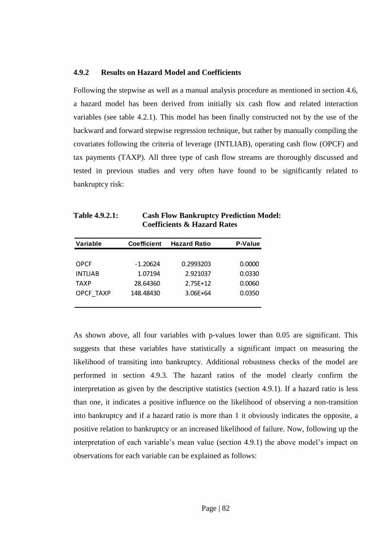
Page | 82
4.9.2 Results on Hazard Model and Coefficients
Following the stepwise as well as a manual analysis procedure as mentioned in section 4.6,
a hazard model has been derived from initially six cash flow and related interaction
variables (see table 4.2.1). This model has been finally constructed not by the use of the
backward and forward stepwise regression technique, but rather by manually compiling the
covariates following the criteria of leverage (INTLIAB), operating cash flow (OPCF) and
tax payments (TAXP). All three type of cash flow streams are thoroughly discussed and
tested in previous studies and very often have found to be significantly related to
bankruptcy risk:
Table 4.9.2.1: Cash Flow Bankruptcy Prediction Model:
Coefficients & Hazard Rates
As shown above, all four variables with p-values lower than 0.05 are significant. This
suggests that these variables have statistically a significant impact on measuring the
likelihood of transiting into bankruptcy. Additional robustness checks of the model are
performed in section 4.9.3. The hazard ratios of the model clearly confirm the
interpretation as given by the descriptive statistics (section 4.9.1). If a hazard ratio is less
than one, it indicates a positive influence on the likelihood of observing a non-transition
into bankruptcy and if a hazard ratio is more than 1 it obviously indicates the opposite, a
positive relation to bankruptcy or an increased likelihood of failure. Now, following up the
interpretation of each variable’s mean value (section 4.9.1) the above model’s impact on
observations for each variable can be explained as follows:
Variable Coefficient Hazard Ratio P-Value
OPCF -1.20624 0.2993203 0.0000
INTLIAB 1.07194 2.921037 0.0330
TAXP 28.64360 2.75E+12 0.0060
OPCF_TAXP 148.48430 3.06E+64 0.0350
Page | 83
OPCF which represents cash flows from operating activities is linked to a hazard ratio of
0.299. For each additional unit of positive cash flow, it is less likely to make the transition
into bankruptcy, which makes perfectly sense also from a valuation point of view. TAXP is
the cash flow component which indicates “Taxes paid”. In this model, observations for
taxes paid are negative numbers. Unless it is a matured start-up company with tax losses to
be carry forward, profitable and cash generating companies pay taxes. This fact should by
intuition result in a negative relation to bankruptcy and therefore in a lowered risk of going
bankrupt. TAXP’s hazard ratio is 2.75e+12 and above 1. The large coefficients on TAXP
and OPCF_TAXP are the function of scale. Therefore, if a company pays high taxes it will
produce a negative TAXP and as such reduce the likelihood of failure. In addition, TAXP
has some incremental explanatory power to OPCF or vice versa. One could argue that
TAXP and OPCF strongly correlate and as such lead to model misspecifications. However,
TAXP gives also some information about a company’s taxable income and related
operating cash flows over time. Start-up companies with significant tax credits to be offset
with future taxable income or restructured companies, which have incurred recurring hefty
losses and negative cash flows followed by profitability are most likely at higher risk than
stable long-lasting cash generating companies. The coefficient may provide this additional
risk content and explanatory power to the model as a whole. Aziz, Emanuel and Lawson
(1988) also found that TAXP was the most important contributor to the model followed by
OPCF, but for all other four variables, ranks were considered to be unstable over time
(Aziz, Emanuel, Lawson 1988). In this study however, another two variables were found to
be significant over the entire time span. INTLIAB which basically reflects the lender’s
cash flow (short-term and long-term debt financing and repayment plus interest payments)
also shows a hazard ratio of more than 1. The excess amount of repayments of debts over
long-term and short-term debts raised is represented by a negative number, which means
that if a company repays its loans on a net basis and if it pays its interest due there is an
increased likelihood to survive. However, if a company raises additional debt, it may help
to stabilize its financial condition on a short-term basis or finance future investments and
anticipated dividend growth. Nevertheless, a company increasing its financial leverage
reflected by a positive INTLIAB is more likely to transition into bankruptcy given the
hazard ratio of 2.92 and its uncertainty of anticipated future dividend growth. It is a
balancing act between leveraging a company and generating sufficient operating cash
flows as reflected by the model’s coefficients. These findings also confirm the results of
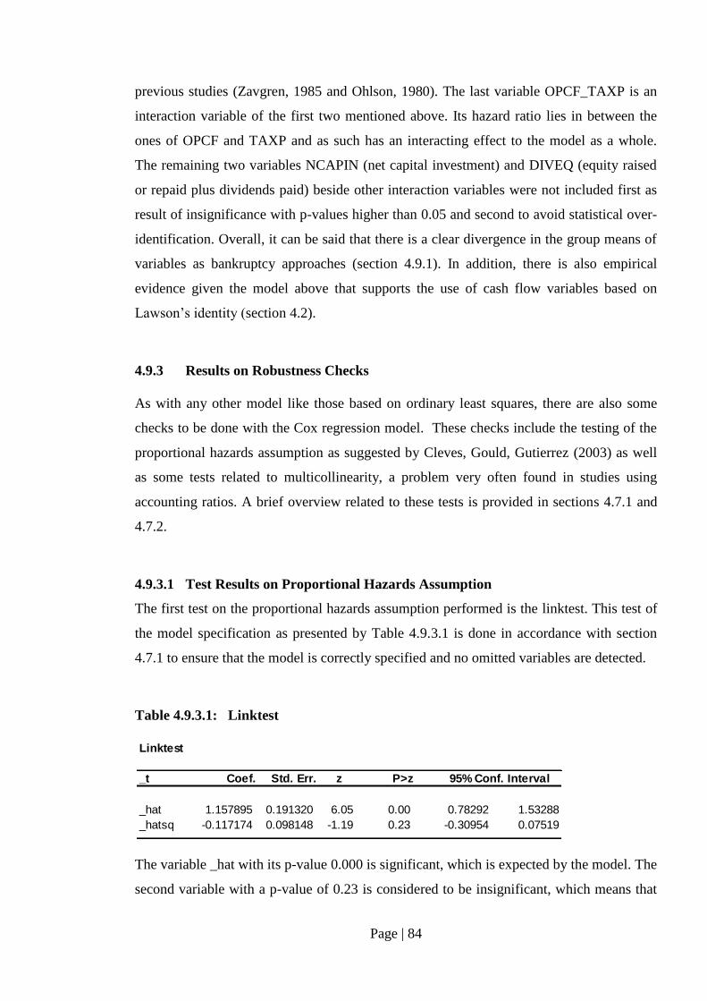
Page | 84
previous studies (Zavgren, 1985 and Ohlson, 1980). The last variable OPCF_TAXP is an
interaction variable of the first two mentioned above. Its hazard ratio lies in between the
ones of OPCF and TAXP and as such has an interacting effect to the model as a whole.
The remaining two variables NCAPIN (net capital investment) and DIVEQ (equity raised
or repaid plus dividends paid) beside other interaction variables were not included first as
result of insignificance with p-values higher than 0.05 and second to avoid statistical over-
identification. Overall, it can be said that there is a clear divergence in the group means of
variables as bankruptcy approaches (section 4.9.1). In addition, there is also empirical
evidence given the model above that supports the use of cash flow variables based on
Lawson’s identity (section 4.2).
4.9.3 Results on Robustness Checks
As with any other model like those based on ordinary least squares, there are also some
checks to be done with the Cox regression model. These checks include the testing of the
proportional hazards assumption as suggested by Cleves, Gould, Gutierrez (2003) as well
as some tests related to multicollinearity, a problem very often found in studies using
accounting ratios. A brief overview related to these tests is provided in sections 4.7.1 and
4.7.2.
4.9.3.1 Test Results on Proportional Hazards Assumption
The first test on the proportional hazards assumption performed is the linktest. This test of
the model specification as presented by Table 4.9.3.1 is done in accordance with section
4.7.1 to ensure that the model is correctly specified and no omitted variables are detected.
Table 4.9.3.1: Linktest
The variable _hat with its p-value 0.000 is significant, which is expected by the model. The
second variable with a p-value of 0.23 is considered to be insignificant, which means that
Linktest
_t Coef. Std. Err. z P>z
_hat 1.157895 0.191320 6.05 0.00 0.78292 1.53288
_hatsq -0.117174 0.098148 -1.19 0.23 -0.30954 0.07519
95% Conf. Interval
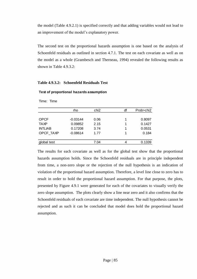
Page | 85
the model (Table 4.9.2.1) is specified correctly and that adding variables would not lead to
an improvement of the model’s explanatory power.
The second test on the proportional hazards assumption is one based on the analysis of
Schoenfeld residuals as outlined in section 4.7.1. The test on each covariate as well as on
the model as a whole (Grambesch and Therneau, 1994) revealed the following results as
shown in Table 4.9.3.2:
Table 4.9.3.2: Schoenfeld Residuals Test
The results for each covariate as well as for the global test show that the proportional
hazards assumption holds. Since the Schoenfeld residuals are in principle independent
from time, a non-zero slope or the rejection of the null hypothesis is an indication of
violation of the proportional hazard assumption. Therefore, a level line close to zero has to
result in order to hold the proportional hazard assumption. For that purpose, the plots,
presented by Figure 4.9.1 were generated for each of the covariates to visually verify the
zero slope assumption. The plots clearly show a line near zero and it also confirms that the
Schoenfeld residuals of each covariate are time independent. The null hypothesis cannot be
rejected and as such it can be concluded that model does hold the proportional hazard
assumption.
Test of proportional hazards assumption
Time: Time
rho chi2 df Prob>chi2
OPCF -0.03144 0.06 1 0.8097
TAXP 0.09852 2.15 1 0.1427
INTLIAB 0.17208 3.74 1 0.0531
OPCF_TAXP -0.08614 1.77 1 0.184
global test 7.04 4 0.1339
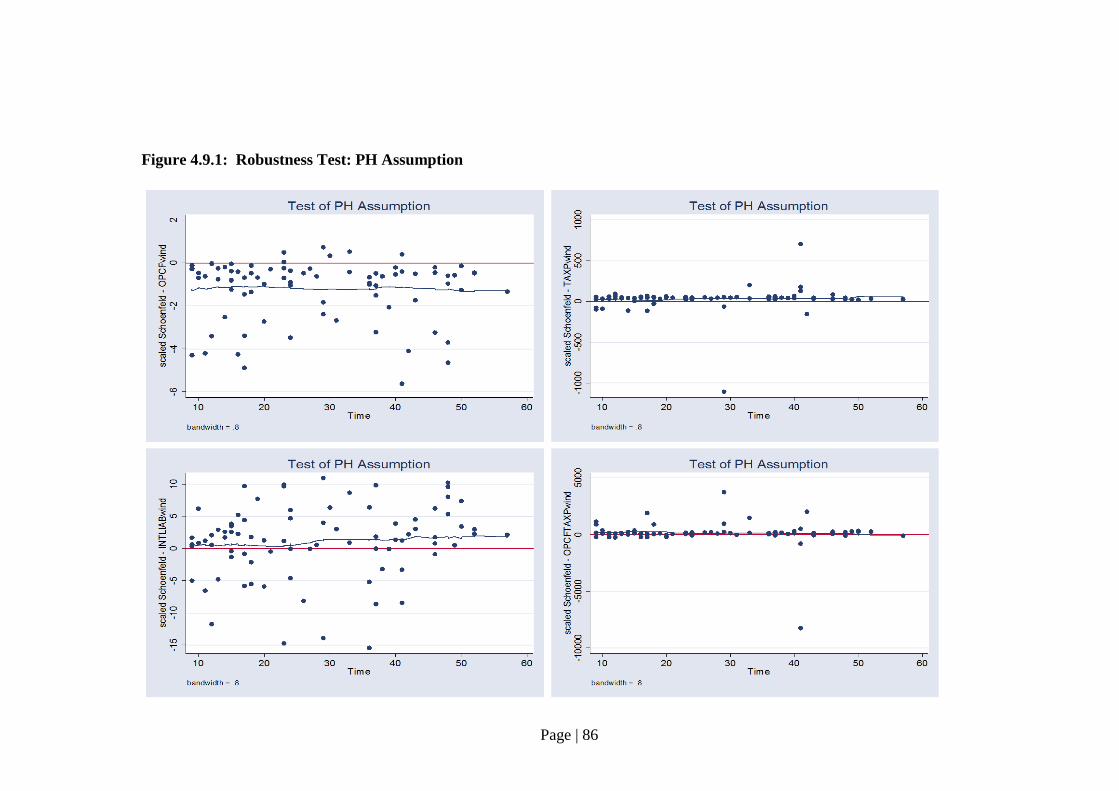
Page | 86
Figure 4.9.1: Robustness Test: PH Assumption
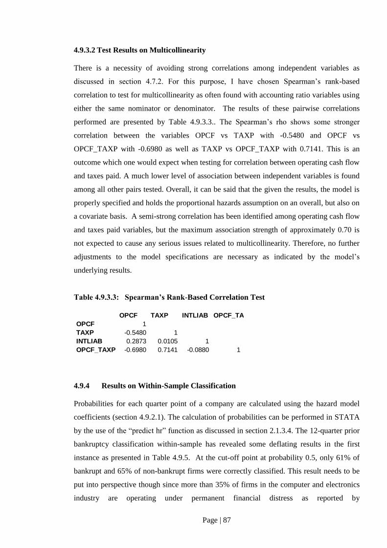
Page | 87
4.9.3.2 Test Results on Multicollinearity
There is a necessity of avoiding strong correlations among independent variables as
discussed in section 4.7.2. For this purpose, I have chosen Spearman’s rank-based
correlation to test for multicollinearity as often found with accounting ratio variables using
either the same nominator or denominator. The results of these pairwise correlations
performed are presented by Table 4.9.3.3.. The Spearman’s rho shows some stronger
correlation between the variables OPCF vs TAXP with -0.5480 and OPCF vs
OPCF_TAXP with -0.6980 as well as TAXP vs OPCF_TAXP with 0.7141. This is an
outcome which one would expect when testing for correlation between operating cash flow
and taxes paid. A much lower level of association between independent variables is found
among all other pairs tested. Overall, it can be said that the given the results, the model is
properly specified and holds the proportional hazards assumption on an overall, but also on
a covariate basis. A semi-strong correlation has been identified among operating cash flow
and taxes paid variables, but the maximum association strength of approximately 0.70 is
not expected to cause any serious issues related to multicollinearity. Therefore, no further
adjustments to the model specifications are necessary as indicated by the model’s
underlying results.
Table 4.9.3.3: Spearman’s Rank-Based Correlation Test
4.9.4 Results on Within-Sample Classification
Probabilities for each quarter point of a company are calculated using the hazard model
coefficients (section 4.9.2.1). The calculation of probabilities can be performed in STATA
by the use of the “predict hr” function as discussed in section 2.1.3.4. The 12-quarter prior
bankruptcy classification within-sample has revealed some deflating results in the first
instance as presented in Table 4.9.5. At the cut-off point at probability 0.5, only 61% of
bankrupt and 65% of non-bankrupt firms were correctly classified. This result needs to be
put into perspective though since more than 35% of firms in the computer and electronics
industry are operating under permanent financial distress as reported by
OPCF TAXP INTLIAB OPCF_TAXP
OPCF 1
TAXP -0.5480 1
INTLIAB 0.2873 0.0105 1
OPCF_TAXP -0.6980 0.7141 -0.0880 1
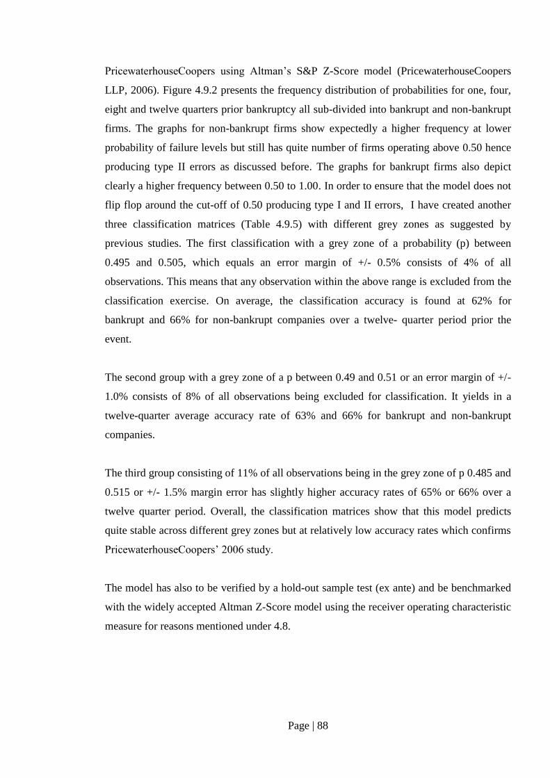
Page | 88
PricewaterhouseCoopers using Altman’s S&P Z-Score model (PricewaterhouseCoopers
LLP, 2006). Figure 4.9.2 presents the frequency distribution of probabilities for one, four,
eight and twelve quarters prior bankruptcy all sub-divided into bankrupt and non-bankrupt
firms. The graphs for non-bankrupt firms show expectedly a higher frequency at lower
probability of failure levels but still has quite number of firms operating above 0.50 hence
producing type II errors as discussed before. The graphs for bankrupt firms also depict
clearly a higher frequency between 0.50 to 1.00. In order to ensure that the model does not
flip flop around the cut-off of 0.50 producing type I and II errors, I have created another
three classification matrices (Table 4.9.5) with different grey zones as suggested by
previous studies. The first classification with a grey zone of a probability (p) between
0.495 and 0.505, which equals an error margin of +/- 0.5% consists of 4% of all
observations. This means that any observation within the above range is excluded from the
classification exercise. On average, the classification accuracy is found at 62% for
bankrupt and 66% for non-bankrupt companies over a twelve- quarter period prior the
event.
The second group with a grey zone of a p between 0.49 and 0.51 or an error margin of +/-
1.0% consists of 8% of all observations being excluded for classification. It yields in a
twelve-quarter average accuracy rate of 63% and 66% for bankrupt and non-bankrupt
companies.
The third group consisting of 11% of all observations being in the grey zone of p 0.485 and
0.515 or +/- 1.5% margin error has slightly higher accuracy rates of 65% or 66% over a
twelve quarter period. Overall, the classification matrices show that this model predicts
quite stable across different grey zones but at relatively low accuracy rates which confirms
PricewaterhouseCoopers’ 2006 study.
The model has also to be verified by a hold-out sample test (ex ante) and be benchmarked
with the widely accepted Altman Z-Score model using the receiver operating characteristic
measure for reasons mentioned under 4.8.
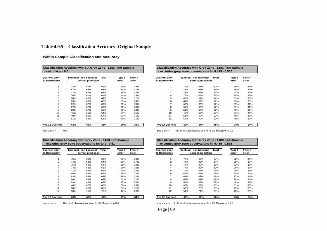
Page | 89
Table 4.9.5: Classification Accuracy: Original Sample
Within-Sample-Classification and Accuracy
Classification Accuracy without Grey Zone - 1183 Firm-Sample Classification Accuracy with Grey Zone - 1183 Firm-Sample
- cut of at p = 0.5 - excludes grey zone observations fm 0.495 - 0.505
Quarters prior bankrupt non-bankrupt Total Type I Type II Quarters prior bankrupt non-bankrupt Total Type I Type II
to Bankruptcy error error to Bankruptcy error error
1 74% 61% 62% 26% 39% 1 74% 61% 62% 26% 39%
2 67% 63% 63% 33% 37% 2 71% 63% 63% 29% 37%
3 72% 62% 63% 28% 38% 3 73% 63% 63% 27% 37%
4 70% 61% 62% 30% 39% 4 72% 62% 62% 28% 38%
5 68% 63% 64% 32% 37% 5 68% 64% 64% 32% 36%
6 65% 66% 66% 35% 34% 6 64% 67% 67% 36% 33%
7 62% 67% 67% 38% 33% 7 63% 68% 67% 37% 32%
8 57% 67% 67% 43% 33% 8 59% 68% 67% 41% 32%
9 50% 67% 65% 50% 33% 9 51% 67% 66% 49% 33%
10 46% 65% 64% 54% 35% 10 49% 66% 65% 51% 34%
11 49% 69% 67% 51% 31% 11 51% 69% 67% 49% 31%
12 51% 69% 68% 49% 31% 12 52% 70% 69% 48% 30%
Avg 12 Quarters 61% 65% 65% 39% 35% Avg 12 Quarters 62% 66% 65% 38% 34%
grey zone = 0% grey zone = 4% of all observations in a +/- 0.5% Margin vs p 0.5
Classification Accuracy with Grey Zone - 1183 Firm-Sample Classification Accuracy with Grey Zone - 1183 Firm-Sample
- excludes grey zone observations fm 0.49 - 0.51 - excludes grey zone observations fm 0.485 - 0.515
Quarters prior bankrupt non-bankrupt Total Type I Type II Quarters prior bankrupt non-bankrupt Total Type I Type II
to Bankruptcy error error to Bankruptcy error error
1 75% 62% 63% 25% 38% 1 78% 62% 63% 22% 38%
2 74% 63% 64% 26% 37% 2 75% 63% 64% 25% 37%
3 75% 62% 63% 25% 38% 3 77% 62% 63% 23% 38%
4 74% 62% 63% 26% 38% 4 74% 63% 63% 26% 37%
5 71% 64% 65% 29% 36% 5 72% 65% 65% 28% 35%
6 65% 68% 68% 35% 32% 6 66% 68% 68% 34% 32%
7 63% 68% 68% 38% 32% 7 63% 69% 68% 37% 31%
8 60% 68% 68% 40% 32% 8 61% 69% 68% 39% 31%
9 53% 68% 67% 47% 33% 9 54% 68% 67% 46% 32%
10 48% 67% 65% 52% 33% 10 49% 67% 66% 51% 33%
11 50% 69% 68% 50% 31% 11 53% 70% 68% 47% 30%
12 53% 71% 70% 47% 29% 12 54% 71% 70% 46% 29%
Avg 12 Quarters 63% 66% 66% 37% 34% Avg 12 Quarters 65% 66% 66% 35% 34%
grey zone = 8% of all observations in a +/- 1% Margin vs p 0.5 grey zone = 11% of all observations in a +/- 1.5% Margin vs p 0.5
correct prediction correct prediction
correct prediction correct prediction
Page | 90
Figure 4.9.2: Frequency Distribution of Probabilities of Original Sample: 1, 4, 8 and
12 Quarters prior Bankruptcy
05
10
15
20
0 .5 1 0 .5 1
bankrupt non-bankrupt
Pe
rcen
t
ProbabilityGraphs by type
1 Quarter prior Bankruptcy - Distribution of Probabilities
05
10
15
20
0 .5 1 0 .5 1
bankrupt non-bankrupt
Pe
rcen
t
ProbabilityGraphs by type
4 Quarter prior Bankruptcy - Distribution of Probabilities0
51
01
5
0 .5 1 0 .5 1
bankrupt non-bankrupt
Pe
rcen
t
ProbabilityGraphs by type
8 Quarter prior Bankruptcy - Distribution of Probabilities
05
10
15
20
0 .5 1 0 .5 1
bankrupt non-bankruptP
erc
en
t
ProbabilityGraphs by type
12 Quarter prior Bankruptcy - Distribution of Probabilities
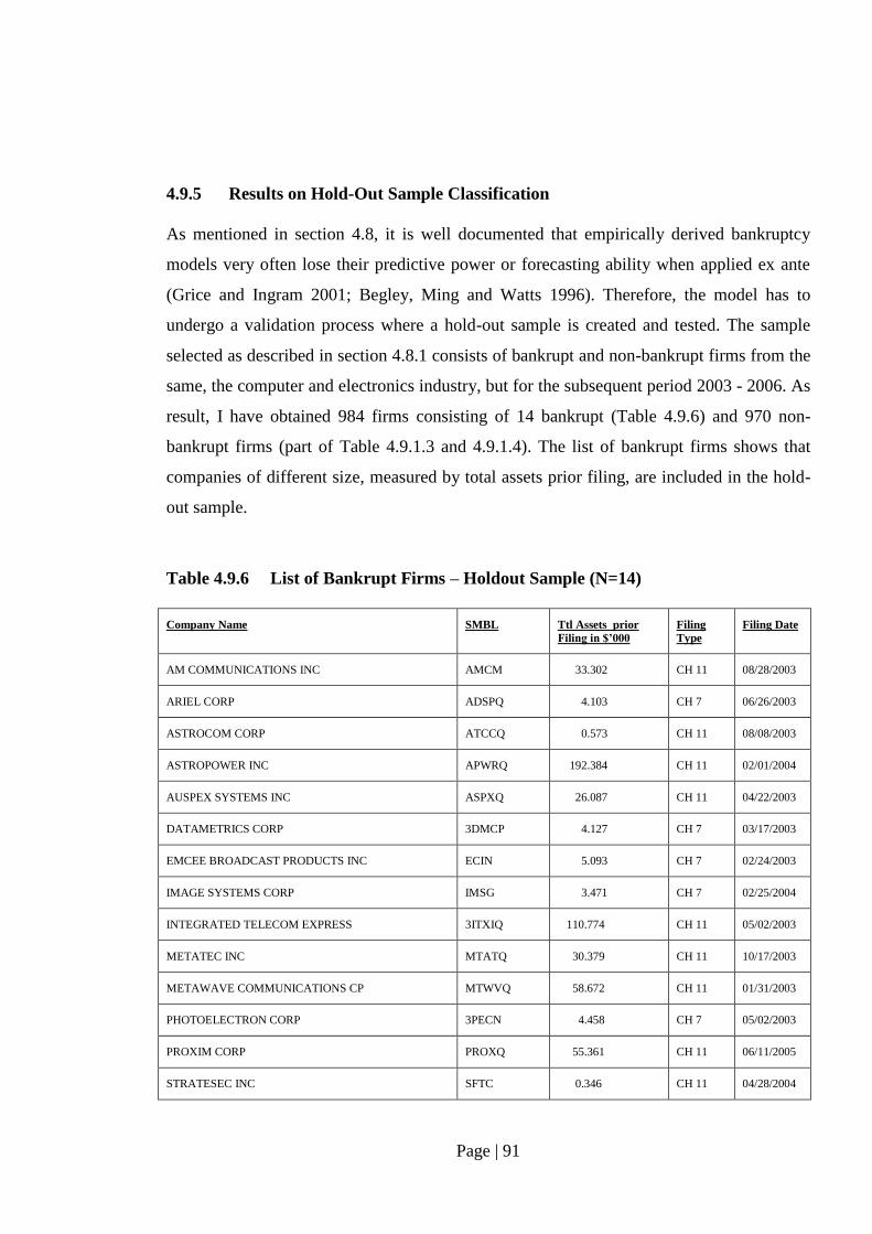
Page | 91
4.9.5 Results on Hold-Out Sample Classification
As mentioned in section 4.8, it is well documented that empirically derived bankruptcy
models very often lose their predictive power or forecasting ability when applied ex ante
(Grice and Ingram 2001; Begley, Ming and Watts 1996). Therefore, the model has to
undergo a validation process where a hold-out sample is created and tested. The sample
selected as described in section 4.8.1 consists of bankrupt and non-bankrupt firms from the
same, the computer and electronics industry, but for the subsequent period 2003 - 2006. As
result, I have obtained 984 firms consisting of 14 bankrupt (Table 4.9.6) and 970 non-
bankrupt firms (part of Table 4.9.1.3 and 4.9.1.4). The list of bankrupt firms shows that
companies of different size, measured by total assets prior filing, are included in the hold-
out sample.
Table 4.9.6 List of Bankrupt Firms – Holdout Sample (N=14)
Company Name SMBL Ttl Assets prior
Filing in $’000
Filing
Type
Filing Date
AM COMMUNICATIONS INC AMCM 33.302 CH 11 08/28/2003
ARIEL CORP ADSPQ 4.103 CH 7 06/26/2003
ASTROCOM CORP ATCCQ 0.573 CH 11 08/08/2003
ASTROPOWER INC APWRQ 192.384 CH 11 02/01/2004
AUSPEX SYSTEMS INC ASPXQ 26.087 CH 11 04/22/2003
DATAMETRICS CORP 3DMCP 4.127 CH 7 03/17/2003
EMCEE BROADCAST PRODUCTS INC ECIN 5.093 CH 7 02/24/2003
IMAGE SYSTEMS CORP IMSG 3.471 CH 7 02/25/2004
INTEGRATED TELECOM EXPRESS 3ITXIQ 110.774 CH 11 05/02/2003
METATEC INC MTATQ 30.379 CH 11 10/17/2003
METAWAVE COMMUNICATIONS CP MTWVQ 58.672 CH 11 01/31/2003
PHOTOELECTRON CORP 3PECN 4.458 CH 7 05/02/2003
PROXIM CORP PROXQ 55.361 CH 11 06/11/2005
STRATESEC INC SFTC 0.346 CH 11 04/28/2004
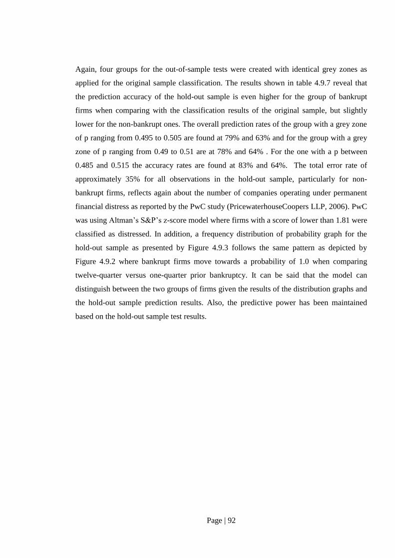
Page | 92
Again, four groups for the out-of-sample tests were created with identical grey zones as
applied for the original sample classification. The results shown in table 4.9.7 reveal that
the prediction accuracy of the hold-out sample is even higher for the group of bankrupt
firms when comparing with the classification results of the original sample, but slightly
lower for the non-bankrupt ones. The overall prediction rates of the group with a grey zone
of p ranging from 0.495 to 0.505 are found at 79% and 63% and for the group with a grey
zone of p ranging from 0.49 to 0.51 are at 78% and 64% . For the one with a p between
0.485 and 0.515 the accuracy rates are found at 83% and 64%. The total error rate of
approximately 35% for all observations in the hold-out sample, particularly for non-
bankrupt firms, reflects again about the number of companies operating under permanent
financial distress as reported by the PwC study (PricewaterhouseCoopers LLP, 2006). PwC
was using Altman’s S&P’s z-score model where firms with a score of lower than 1.81 were
classified as distressed. In addition, a frequency distribution of probability graph for the
hold-out sample as presented by Figure 4.9.3 follows the same pattern as depicted by
Figure 4.9.2 where bankrupt firms move towards a probability of 1.0 when comparing
twelve-quarter versus one-quarter prior bankruptcy. It can be said that the model can
distinguish between the two groups of firms given the results of the distribution graphs and
the hold-out sample prediction results. Also, the predictive power has been maintained
based on the hold-out sample test results.
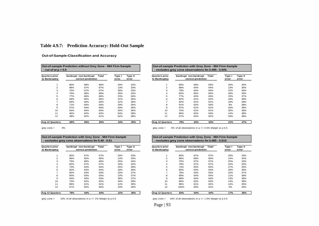
Page | 93
Table 4.9.7: Prediction Accuracy: Hold-Out Sample
Out-of-Sample-Classification and Accuracy
Out-of-sample Prediction without Grey Zone - 984 Firm-Sample Out-of-sample Prediction with Grey Zone - 984 Firm-Sample
- cut of at p = 0.5 - excludes grey zone observations fm 0.495 - 0.505
Quarters prior bankrupt non-bankrupt Total Type I Type II Quarters prior bankrupt non-bankrupt Total Type I Type II
to Bankruptcy error error to Bankruptcy error error
1 80% 68% 68% 20% 32% 1 80% 65% 65% 20% 35%
2 88% 67% 67% 13% 33% 2 88% 64% 64% 13% 36%
3 70% 67% 67% 30% 33% 3 78% 64% 64% 22% 36%
4 75% 68% 68% 25% 32% 4 82% 65% 65% 18% 35%
5 77% 66% 66% 23% 34% 5 77% 63% 63% 23% 37%
6 69% 65% 65% 31% 35% 6 82% 61% 62% 18% 39%
7 69% 64% 64% 31% 36% 7 82% 61% 61% 18% 39%
8 71% 65% 65% 29% 35% 8 91% 62% 63% 9% 38%
9 57% 64% 64% 43% 36% 9 67% 61% 61% 33% 39%
10 50% 64% 63% 50% 36% 10 70% 61% 61% 30% 39%
11 46% 62% 62% 54% 38% 11 86% 62% 63% 14% 38%
12 38% 62% 61% 62% 38% 12 67% 62% 62% 33% 38%
Avg 12 Quarters 66% 65% 65% 34% 35% Avg 12 Quarters 79% 63% 63% 21% 37%
grey zone = 0% grey zone = 5% of all observations in a +/- 0.5% Margin vs p 0.5
Out-of-sample Prediction with Grey Zone - 984 Firm-Sample Out-of-sample Prediction with Grey Zone - 984 Firm-Sample
- excludes grey zone observations fm 0.49 - 0.51 - excludes grey zone observations fm 0.485 - 0.515
Quarters prior bankrupt non-bankrupt Total Type I Type II Quarters prior bankrupt non-bankrupt Total Type I Type II
to Bankruptcy error error to Bankruptcy error error
1 80% 67% 67% 20% 33% 1 80% 67% 67% 20% 33%
2 86% 65% 66% 14% 35% 2 86% 66% 66% 14% 34%
3 75% 66% 66% 25% 34% 3 75% 67% 67% 25% 33%
4 82% 67% 67% 18% 33% 4 78% 67% 67% 22% 33%
5 75% 64% 64% 25% 36% 5 73% 65% 65% 27% 35%
6 82% 64% 64% 18% 36% 6 80% 64% 64% 20% 36%
7 80% 63% 63% 20% 37% 7 78% 63% 63% 22% 37%
8 90% 63% 63% 10% 37% 8 89% 64% 64% 11% 36%
9 64% 63% 63% 36% 37% 9 88% 64% 64% 13% 36%
10 70% 62% 62% 30% 38% 10 86% 62% 63% 14% 38%
11 86% 61% 61% 14% 39% 11 86% 61% 62% 14% 39%
12 67% 60% 60% 33% 40% 12 100% 60% 61% 0% 40%
Avg 12 Quarters 78% 64% 64% 22% 36% Avg 12 Quarters 83% 64% 64% 17% 36%
grey zone = 10% of all observations in a +/- 1% Margin vs p 0.5 grey zone = 14% of all observations in a +/- 1.5% Margin vs p 0.5
correct prediction correct prediction
correct prediction correct prediction
Page | 94
Figure 4.9.3: Frequency Distribution of Probabilities of Hold-Out Sample: 1, 4, 8 and
12 Quarters prior Bankruptcy
01
02
03
04
0
0 .5 1 0 .5 1
bankrupt non-bankrupt
Pe
rcen
t
ProbabilityGraphs by type
1 Quarter prior Bankruptcy - Distribution of Probabilities
01
02
03
0
0 .5 1 0 .5 1
bankrupt non-bankrupt
Pe
rcen
t
ProbabilityGraphs by type
4 Quarter prior Bankruptcy - Distribution of Probabilities0
10
20
30
40
0 .5 1 0 .5 1
bankrupt non-bankrupt
Pe
rcen
t
ProbabilityGraphs by type
8 Quarter prior Bankruptcy - Distribution of Probabilities
02
04
06
08
0
0 .5 1 0 .5 1
bankrupt non-bankruptP
erc
en
t
ProbabilityGraphs by type
12 Quarter prior Bankruptcy - Distribution of Probabilities
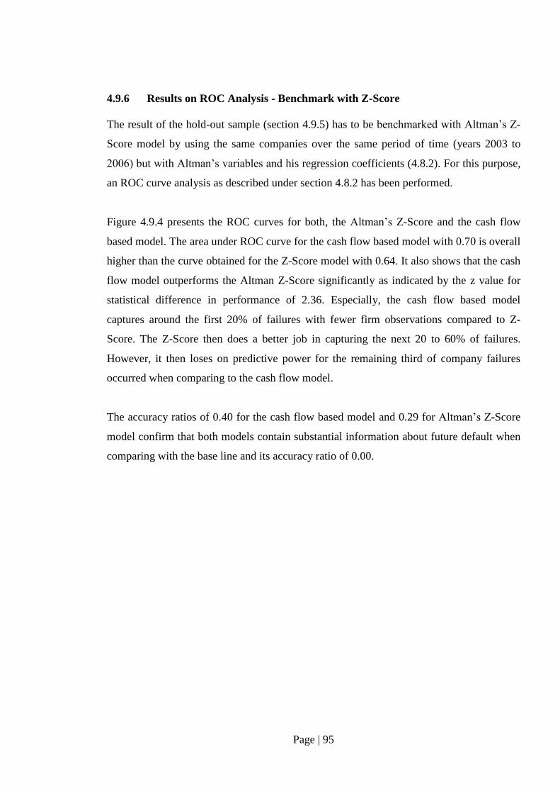
Page | 95
4.9.6 Results on ROC Analysis - Benchmark with Z-Score
The result of the hold-out sample (section 4.9.5) has to be benchmarked with Altman’s Z-
Score model by using the same companies over the same period of time (years 2003 to
2006) but with Altman’s variables and his regression coefficients (4.8.2). For this purpose,
an ROC curve analysis as described under section 4.8.2 has been performed.
Figure 4.9.4 presents the ROC curves for both, the Altman’s Z-Score and the cash flow
based model. The area under ROC curve for the cash flow based model with 0.70 is overall
higher than the curve obtained for the Z-Score model with 0.64. It also shows that the cash
flow model outperforms the Altman Z-Score significantly as indicated by the z value for
statistical difference in performance of 2.36. Especially, the cash flow based model
captures around the first 20% of failures with fewer firm observations compared to Z-
Score. The Z-Score then does a better job in capturing the next 20 to 60% of failures.
However, it then loses on predictive power for the remaining third of company failures
occurred when comparing to the cash flow model.
The accuracy ratios of 0.40 for the cash flow based model and 0.29 for Altman’s Z-Score
model confirm that both models contain substantial information about future default when
comparing with the base line and its accuracy ratio of 0.00.
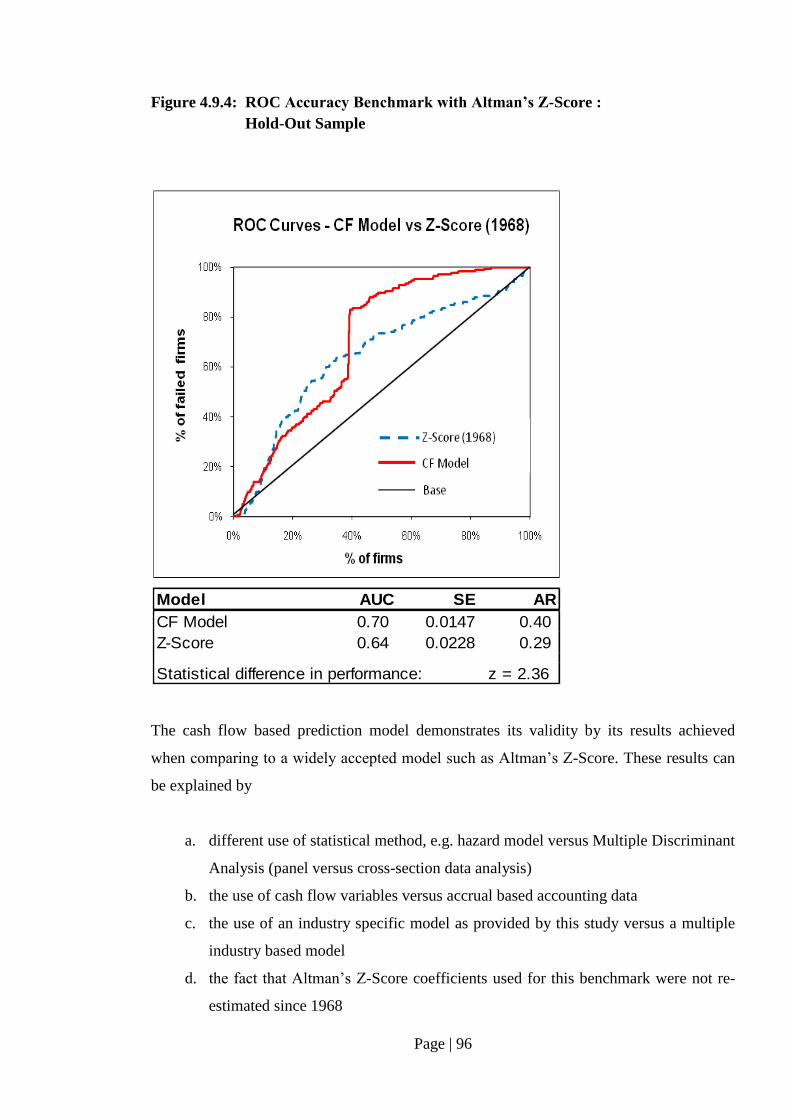
Page | 96
Figure 4.9.4: ROC Accuracy Benchmark with Altman’s Z-Score :
Hold-Out Sample
The cash flow based prediction model demonstrates its validity by its results achieved
when comparing to a widely accepted model such as Altman’s Z-Score. These results can
be explained by
a. different use of statistical method, e.g. hazard model versus Multiple Discriminant
Analysis (panel versus cross-section data analysis)
b. the use of cash flow variables versus accrual based accounting data
c. the use of an industry specific model as provided by this study versus a multiple
industry based model
d. the fact that Altman’s Z-Score coefficients used for this benchmark were not re-
estimated since 1968
Model AUC SE AR
CF Model 0.70 0.0147 0.40
Z-Score 0.64 0.0228 0.29
Statistical difference in performance: z = 2.36
Page | 97
e. the fact that Altman’s model was based on much fewer companies and related
observations
f. the development of a quarterly moving average full year model in this study
versus a year-end annual model as used by Altman and others
g. the fact that the dichotomy of bankrupt versus non-bankrupt may slightly differ
between the two models, e.g. new bankruptcy code of 1978. Altman’s model was
created with data prior this new code in contrast to this study.
Since it is not the ultimate goal to find the most influential factor in improving accuracies
of bankruptcy predictions, I will not analyze this subject any further. The use of a multi-
period hazard model appears to be a more appropriate statistical method though than a
single-period static MDA model as used by Altman.
4.9.7 Results on Continuous Distress Risk Tabulation
The characteristic of the distress risk measure has been evaluated by tabulating the
probability of default deciles against the failure rates as described under 4.8.3. As per
figure 4.9.5 and the strong correlation of 0.9168 between the probability of failure and the
number of failures it is evident that the cash flow based bankruptcy prediction model
produces a continuous distress factor. Therefore, the probabilities of failure obtained from
the cash flow prediction model can be included as a continuous pricing factor into the asset
pricing models as shown in chapter 5.
Page | 98
Figure 4.9.5: Probability of Default Deciles vs Failure Rates
4.10 Bankruptcy Prediction Model: Summary Result and Conclusion
The bankruptcy prediction model using cash flow variables based on Lawson’s Identity has
brought up four variables of significance. Also, it is not of surprise that cash flows related
to operating activities (OPCF), taxes (TAXP) as well as leverage and interest paid
(INTLIAB) offer the most significant predictors from a bankruptcy risk point of view as
these factors are very much related to a firm’s valuation. The model has also shown that
cash flows related to net capital investment (NCAPIN), the equity (DIVEQ) and change in
liquidity (CHLIQ) do not contribute significantly to the model as a whole. The new cash
flow based prediction model has been validated by robustness checks, hold-out sample
tests and by a ROC benchmark with Altman’s Z-Score model. The twelve-quarter average
overall accuracy rates from within-sample classifications are in the range of 65% to 66%
and confirm a) the stability of the model and b) the PricewaterhouseCoopers (2006) study.
Figure 4.9.2 depicts the fact that the model is able to segregate between the groups of
bankrupt and non-bankrupt firms. Although the test results are rather modest (section 4.9.4)
it can be concluded that hypothesis H1Aa) (see section 3.2 and paragraph below) shown in
0
10
20
30
40
50
60
70
80
90
0
5
10
15
20
25
30
35
40
45
50
1 2 3 4 5 6 7 8 9 10
# o
f Fa
ilure
s b
y D
eci
le
Probability of Default Deciles
Number of Failures by Probability of Default Deciles
Failure Rate
Accumulated Failure Rate
# o
f ac
cum
.Fa
ilure
s
Correlation Maxtrix:
Probability # of Failure
Probability 1.0000
# of Failure 0.9168 1.0000
Page | 99
alternative form below cannot be rejected, which means that the model as stated under
H1Aa) below can predict the failure or non-failure of firms at relatively low type I and II
error rates. It has to be put in perspective with the situation of this specific industry as
reported by PricewaterhouseCoopers (2006) where 35% of firms are found to be operating
under permanent distress. The benchmark test with Altman’s Z-score will reveal the
model’s underlying value.
H1Aa) A dynamic cash flow based bankruptcy prediction model can predict the
failure or non-failure of firms at low type I and II error rates based on within-
sample classification (section 4.9.4)
The test results (section 4.9.3) from the model’s robustness checks confirm that the model
holds the proportional hazards assumption and also that it is not subject to the issue of
multicollinearity. In addition, the out-of-sample tests as performed in section 4.9.5 show
that the new cash flow based model is able to maintain its predictive power given its
accuracy rates over the twelve-quarter period prior bankruptcy. The overall rate is found to
be between 63% and 65% depending on the grey zone definition. Figure 4.9.3 again
depicts the fact that the model can categorize into the two groups bankrupt and non-
bankrupt. The ROC benchmark test results with Altman’s Z-Score (section 4.9.6) also
confirm the model’s validity. The area under ROC curve for the cash flow based model is
overall higher than the curve obtained for the Z-Score model. In addition, the cash flow
model outperforms the Altman Z-Score significantly as indicated by the z value for
statistical difference in performance. Given the fact that the cash flow based prediction
model is robust and more accurate in comparison to Altman’s Z-Score it can be concluded
that hypothesis H1Ab) (see section 3.2 and paragraph below) cannot be rejected, which
means that the model maintains its predictive power in hold-out sample tests and that it
performs better than the Z-Score model, at least for bankruptcy predictions in the computer
and electronics equipment industry. The probabilities obtained from this model can be used
for further asset pricing tests (5.1).
H1Ab) A dynamic cash flow based bankruptcy prediction model can predict the
failure or non-failure of firms from out-of-sample tests (section 4.9.5) at the same
or higher accuracy rate compared to the existing and widely accepted Z-Score
Model (section 4.9.6) by using a ROC-model, and as such be used for further
asset pricing tests (chapter 5).
Page | 100
The characteristic of the distress risk measure has been evaluated by tabulating the
probability of default deciles against the failure rates. Figure 4.9.5 and the strong
correlation of 0.9168 between the probability of failure and the number of failures show
that it is evident that the cash flow based bankruptcy prediction model produces a
continuous distress factor. Hence, H1Ac) cannot be rejected and the probabilities obtained
from the bankruptcy prediction model can be used as continuous distress risk factor for
further asset pricing tests (5.1).
H1Ac) A dynamic cash flow based bankruptcy prediction model produces
continuous probabilities of default measure (sections 4.8.3 / 4.9.7)
Page | 101
CHAPTER 5: ASSET PRICING OF PROFITABILITY AND
RELATIVE DISTRESS RISK
5.1 Overview
In order to test for the hypotheses set in section 5.2 (or 3.3). several tasks will need to be
performed. First, various portfolios as described in section 5.5.1 are formed and factors
calculated on an equal-weighted basis. The portfolios are rebalanced on a quarterly basis
using only publicly available data at the formation date. Therefore, a three-month reporting
lag is assumed to avoid any look-ahead bias (Banz and Breen, 1996). The descriptive
statistics emerged from the portfolio formation and factor calculations based on time-series
averages over 204 months (1990 – 2006) and are provided for distress deciles sorted as
well as for size-B/M-distress sorted portfolios in section 5.6.1 and for additional portfolio
sorts in Appendix A. The descriptive statistics are reported in raw numbers (tables) and
supplemented by graphs (figures) with corresponding comments and analyses. In section
5.6.2, Pearson correlation tests are conducted to check if all explaining variables are
independent from each other and to obtain results in connection with the Fama-French
(1992, 1993) distress factor hypothesis. Last but not least, Fama-MacBeth (1973) cross-
sectional regressions are run on various sets of portfolios (section 5.6.3) to obtain t-
statistics and adj. R2 for different types of models such as CAPM, Fama-French (1992)
three-factor model and augmentations of it including the relative distress risk and current
profitability strength (OPCF) factors and related interaction term.
5.2 Hypotheses
The reasoning for the hypotheses below is provided in section 3.3.
H2Aa) Distressed stocks underperform on average non-distressed stocks. (descriptive
statistics 5.6.1, Table 5.6.1.1 and 5.6.4)
H2Ab): The Fama-French (1992, 1993) distress factor hypothesis where both size and
B/M factors proxy distress risk does not hold. (Descriptive Statistics 5.6.1, figure 5.6.1.4 /
Pearson’s rank correlation: test outline 5.5.3 and test results 5.6.2 / Cross-sectional
regression: test outline 5.5.4 and test results 5.6.3)
Page | 102
H2Ac): The anomalous market underperformance of distressed stock can be explained
by a parallel analysis of risk based rational pricing and profitability/earnings levels to
returns propositions. (Descriptive statistics 5.6.1, Table 5.6.1.1,5.6.1.6, Figure 5.6.1.1,
5.6.1.6, 5.6.1.33) / Cross-sectional regression: test outline 5.5.4 and test results 5.6.3)
5.3 Data Source
Data for monthly stock returns are downloaded from the Wharton Research Data Service –
Center for Research in Security Prices (CRSP) database. The monthly distress factors
derived from the quarterly cash flow based bankruptcy prediction model are obtained from
the calculations as described in chapter 4. The probabilities of bankruptcy are calculated on
a quarterly basis. The same probability is assigned to each month within a quarter, e.g.
January, February and March will have the same distress factor and will then be adjusted
for the next three months and so forth.
5.4 Sample Selection
The sample will include all bankrupt and non-bankrupt companies as selected for the
bankruptcy prediction model. Companies with the following NAICS Codes (North
American Industry Classification System) are included:
334 Computer and Electronic Product Manufacturing
3341 Computer and Peripheral Equipment Manufacturing
3342 Communications Equipment Manufacturing
3344 Semiconductor and Other Electronic Component Manufacturing
3345 Navigational, Measuring, Medical and Control Instruments Manufacturing
The disclosure of Statement of Cash Flows was optional until SFAS No. 95 became a
mandatory requirement in 1988. Therefore, the sample for the asset pricing tests will
include monthly data for the period when distress factors became available, starting in year
1990 and ending in 2006. In addition, the sample size used to develop and test the
bankruptcy prediction model is reduced by the fact that for asset pricing tests firms listed
on the NYSE, AMEX and NASDAQ stock exchanges are included only. Although
OTCBB stocks have to the meet the same SEC reporting standards and requirements they
very often are the ones which were delisted from NYSE, AMEX or NASDAQ stock
Page | 103
exchanges due to undercapitalization, small share price and other reasons. Subsequently,
OTCBB stocks often file for bankruptcy Chapter 11 or 7 and as such have rightly been
used for the development of the cash flow based bankruptcy prediction model in chapter 4.
Nevertheless, OTCBB stocks are dropped due to unavailability of data (CRSP) and
because of being subject to a potential thin trading problem.
The inclusion of stocks has to meet further criteria similar to the ones defined by Agarwal
and Taffler (2008) and Campell, Hilscher and Szilagyi (2008). Stocks with a negative
book-to-market ratio are excluded as its interpretation is rather difficult. The thin trading
issue has been also considered for NYSE, AMEX and NASDAQ listed companies. In
contrast to other studies (Agarwal and Taffler, 2008; Campbell, Hilscher, Szilagyi, 2008),
portfolios are formed and rebalanced on a quarterly basis at the beginning of each quarter.
Therefore, stocks which have not been traded in all three months of a quarter are excluded
unless they were delisted before quarter end. However, almost no thin trading has been
noted and thus it does not pose any serious problem for this study. As result, a total of
1’236 firms which corresponds to 112’631 firm months over the entire period or 520 firms
on average per month are included in the sample to be tested.
Delisted returns provided by CRSP are used whenever available for companies being
delisted. There are only a few instances where the latest available full month return is used
instead.
5.5 Methodology, Design and Models
5.5.1 Portfolio Formation and Calculations
Different sets of portfolios are formed to test the hypotheses (section 5.2) and to validate
the outcome. All characteristics used for portfolio formation as well as the calculations of
returns and factors are equally weighted. The portfolios’ characteristics are shown in form
of descriptive statistics (section 5.5.2) and have to undergo correlations tests as shown in
section 5.5.3. Cross-sectional regression tests (section 5.5.3) are run and t-statistics are
provided by applying the Fama-MacBeth (1973) two-stage regression methodology. This
study is limited to one industry and as consequence it deals with a fewer number of stocks
compared to many other studies covering the market as a whole. Four- or three-way
intersecting portfolios are preferred over two-way intersecting ones given the number of
characteristics used in this study. However, the implementation of four-way intersecting
Page | 104
portfolios is not feasible as it would drive down the number of stocks per portfolio too
often below ten. Therefore, one set of three-way intersecting portfolios is formed to
control for two characteristics at a given time. The characteristics used for these portfolios
are distress risk, B/M and Size but not OPCF. As compromise, the OPCF characteristic is
used in a two-way independent sort together with distress risk. Since I also test the Fama-
French (1992) factors for their level of significance, I have also chosen to test two-way
intersecting portfolios by the inclusion of a finer grid of B/M and size characteristics which
are compromised when using three-way intersecting portfolios. I have chosen B/M and
Size quartiles sorts for two-way intersecting portfolios and for both characteristics a
breakpoint at the median for three-way intersecting portfolios. This allows maintaining a
minimum number of stocks per portfolio and per period for the sets of portfolios to be
formed. The independent sorting of stocks into distress risk deciles and quintiles instead of
quartiles has some analytical reasons. From the 8th
to the 9th
decile or from the 4th
to the 5th
quintile the average probability of failure is switching from a lesser to a more likelihood of
going bankrupt. This switching point would not have been visible with distress risk sorted
by quartiles instead.
1. Distress deciles sorted portfolio
The distress deciles sorted portfolios are calculated and rebalanced on a quarterly
basis. This set of portfolios (Table 5.6.1.1) is formed for descriptive statistics
purpose only. Most important, it provides the monthly excess returns across the
distress risk levels on an equal-weighted basis. In addition, this one-way sort of
relative distress risk provides a finer grid of this characteristic compared to all other
portfolios formed in this study. This analysis also provides the average stock
returns across distress deciles and the information needed in connection with
hypothesis H2Aa).
2. Two-way intersecting portfolios (Appendix A)
Four sets of two-way intersecting portfolios are formed to control the distress factor
by each of the other characteristics on an individual basis. Distress risk quintiles
instead of deciles are used in order to ensure a minimum number of stocks per
portfolio per period. The first set of 20 portfolios (Table 5.6.1.2, Appendix A)
consists of Distress risk quintiles and OPCF quartiles constructed at their
Page | 105
intersections (Distress (5) * OPCF (4)). This is the only portfolio formation that is
not based on stock price transformation and the only set consisting of OPCF sorted
portfolios. It reveals that distress risk controlled by profitability (OPCF) tends to be
positive nearly linear in relation to monthly excess returns. The second set of 20
portfolios (Table 5.6.1.3, Appendix A) consists of Distress risk quintiles and Size
quartiles (Distress (5) * Size (4)). The third set (Table 5.6.1.4, Appendix A)
consists of Distress risk quintiles and B/M quartiles (Distress (5) * B/M (4)). The
fourth set of 16 portfolios (Table 5.6.1.5, Appendix A) consists of Size and B/M
quartiles (Size (4) * B/M (4)). All two-way intersecting portfolios are formed,
calculated and rebalanced on a quarterly basis and equal-weighted.
3. Three-way intersecting portfolios
There is one set of three-way intersecting portfolios constructed (Table 5.6.1.6).
Here, the distress portfolios are controlled by Size and B/M characteristics. In
order to maintain a minimum number of stocks in each portfolio and period, I use
Size and B/M halves with breakpoints at their median. This independent portfolio
sorting and formation method results in 20 portfolios (Distress (5) * Size (2) * B/M
(2)). The three-way intersecting portfolios are formed, calculated and rebalanced on
a quarterly basis and equal-weighted.
4. Distress Decile Portfolio by Positive / Negative OPCF
OPCF reflects a company’s scaled operating cash flow before interest and taxes
paid. The Distress risk deciles will be segregated into positive and negative OPCF
stocks (Figure 5.6.1.33), which reveals additional descriptive information on the
interaction between Distress risk and OPCF as well as their relationship with
returns, especially at highest distress risk levels.
5. Calculation of Returns and Factors
The stocks of the entire sample as defined and selected in section 5.4 will be
grouped into various sets of portfolios of independent sorts (see 1. – 4. above). The
descriptive statistics (section 5.5.2) and the cross-sectional regression analysis
(section 5.5.3) are based on the Fama and MacBeth (1973) methodology. The
Page | 106
calculation of factors and returns are the same for all portfolios and equally-
weighted.
Rit – RFt = it + 1tit-1 + 2t ln(sizeit-1) + 3t ln(B/Mit-1) + 4t (distressit-1) + 5t (OPCFit-1) + it
where:
Rit is the equal-weighted return on portfolio i during month t
RFt is the one month t-bill rate at the beginning of each month t
it-1 is the beta of portfolio i estimated at the portfolio formation
date using a rolling 24-month window prior to formation date
(further details see section 2.2.3.2)
ln(sizeit-1) is the natural logarithm of the average market capitalization of
equity stocks in portfolio i at the portfolio formation date t-1
ln(B/Mit-1) is the natural logarithm of the average B/M ratios of stocks in
portfolio i at the portfolio formation date t-1 1
(distressit-1) is the distress risk factor proxied by the probability of bankruptcy
risk (Chapter 4) of portfolio i at portfolio formation date 1
(OPCFit-1) is a scaled accumulated four-quarter profitability coefficient
derived from the bankruptcy prediction model for portfolio i at
the portfolio formation date 1
it is a mean-zero stochastic error term
Book Equity (B/) is the book value of common stock plus balance-sheet deferred taxes.
Values being lower than the 1st percentile and higher than the 99
th percentile will be set to
the values of 1st or 99
th percentile of observations in order to eliminate extreme outliers.
Rebalancing of portfolios occurs at the beginning of each quarter.
1 There is a 3-month reporting lag assumed to avoid any look-ahead bias (Banz and Breen, 1996). 92% of companies
filed annual reports within 3 months (Penman, 1987) and 98% with 5 months (Alford, Jones, Zmijewski, 1994).
Tests on 4- and 5-month lag models have shown a diminishing level of statistical significance. 6-month lag led to an
overall insignificance of factors and models involved.
5.5.2 Descriptive Statistics
Descriptive statistics and related figures including comments are provided for all sets of
portfolios (5.5.1) as listed below:
Portfolio Set Table Figures
Distress Risk Probability Decile Portfolios 5.6.1.1 5.6.1.1 to 5.6.1.6

Page | 107
Size Median * B/M Median * Distress Quintiles 5.6.1.6 5.6.1.29 to 5.6.1.32
Portfolio Sets in APPENDIX A:
OPCF Quartiles * Distress Quintiles 5.6.1.2 5.6.1.7 to 5.6.1.10
Size Quartiles * Distress Quintiles 5.6.1.3 5.6.1.11 to 5.6.1.16
B/M Quartiles * Distress Quintiles 5.6.1.4 5.6.1.17 to 5.6.1.22
Size Quartiles * B/M Quartiles 5.6.1.5 5.6.1.23 to 5.6.1.28
For each portfolio of the above sets of portfolios the following descriptive statistics are
provided:
Panel A.: Monthly Mean Excess Return
Panel B: Mean Beta
Panel C: Mean ln(Size)
Panel D: Mean ln(B/M)
Panel E: Mean Distress Probability
Panel F: Mean OPCF
Panel G: Average Size – Market Cap in $m
Panel H: Average Number of Stocks (per month)
Besides providing a descriptive overview of the mean statistics for differently formed
portfolios based on various characteristics, it also is used for testing the hypothesis H2Aa)
as described in sections 3.3.
5.5.3 Multicollinearity Tests
One problem, which potentially could arise, is multicollinearity among independent
variables since financial ratios have quite often the same numerator or denominator. If
there were multiple highly correlated covariates, it is preferred to include only one variable
from the set of correlated variables. Therefore, Pearson’s rank correlation tests are
conducted for each pair of variable. In a perfect world, all independent variables would be
completely independent and unrelated to each other, but reality shows though that virtually
every multiple regression has some collinearity between the independent covariates. There
are no clear-cut rules about the level of collinearity to be excluded from a model, but if it
Page | 108
exceeds 0.80 it would probably make sense to drop one of the highly correlated variables.
In addition, these correlation tests are also used to evaluate the distress factor proposition
made by Fama and French (1992) and Chan and Chen (1991). In their studies they argue
that size and B/M factors in a multi-factor asset pricing framework proxy for bankruptcy
risk (further details see 2.2.4). Assuming that the distress risk factor derived from the
bankruptcy prediction model is valid and the Fama-French distress factor hypothesis is
considered to be true, the correlation particularly between B/M and the distress risk factor
is expected to be very strong. For this specific purpose (hypothesis H2Ab), sections 3.3 or
5.2) the correlations among these variables for individual stocks (Table 5.6.2.1, Appendix
B) but also for the following portfolios are tested:
Portfolio Set Table
Size Median * B/M Median * Distress Quintiles 5.6.2.4
Portfolio Sets in APPENDIX B:
OPCF Quartiles * Distress Quintiles 5.6.2.2
Size Quartiles * Distress Quintiles 5.6.2.3
B/M Quartiles * Distress Quintiles 5.6.2.5
The tests are performed on a monthly basis. The correlation coefficients
reported in the tables above are the time-series average of 204 months.
5.5.4 Cross-Sectional Regression Tests
The descriptive statistics provided in section 5.5.2 describes specifically the mean statistics
of all characteristics involved in forming the various sets of portfolios and eventually
explaining monthly average stock returns. Besides the first findings from the descriptive
statistics I also test for the factors’ and the models’ significance levels in explaining the
monthly excess stock returns related to hypotheses H2Aa) and H2Ac) (see details in sections
5.2 and/or 3.3). For that purpose I apply the Fama and MacBeth (1973) cross-sectional
regression methodology which is discussed in more details in section 2.2.3.2. The
following sets of portfolios’ monthly excess stock returns will be tested:
Page | 109
Portfolio Set Descriptive
Table No.
Regression
Table No.
Size Median * B/M Median * Distress Quintiles 5.6.1.6 5.6.3.4
Portfolio Sets in APPENDIX C:
OPCF Quartiles * Distress Quintiles 5.6.1.2 5.6.3.1
Size Quartiles * Distress Quintiles 5.6.1.3 5.6.3.2
B/M Quartiles * Distress Quintiles 5.6.1.4 5.6.3.3
Size Quartiles * B/M Quartiles 5.6.1.5 5.6.3.5
As a robustness check, all asset pricing tests are also conducted with individual securities’
regressions. The use of individual securities (Chan, Hamao, Lakonishok, 1991) is aimed to
disprove the claim of the data snooping bias (Lo and MacKinlay, 1990; Black, 1993,
MacKinlay, 1995) (see section 2.2.3.4).
Portfolio Set – Robustness Checks Regression Table No.
Individual Stock Regression 5.6.3.6
Most of the empirical validations of the CAPM are conducted based on studies related to
Fama and French’s (1992, 1993) three-factor model. Several modified versions of the
three-factor model are tested on a univariate as well as multivariate basis. Beta, the market
factor, remains a factor for all models to be included in this study because of its strong
theoretical framework except for the testing of the interaction term (model 12).
The following models are tested:
CAPM
1. Rit – RFt = it + 1tit-1 + it
Fama & French 3-Factor (1992)
2. Rit – RFt = it + 1tit-1 + 2t ln(sizeit-1) + 3t ln(B/Mit-1) + it
Multi-Factor
3. Rit – RFt = it + 1tit-1 + 2t ln(sizeit-1) + 3t ln(B/Mit-1) + 4t (distressit-1) + it
4. Rit – RFt = it + 1tit-1 + 2t ln(sizeit-1) + 3t ln(B/Mit-1) + 5t (OPCFit-1)+ it
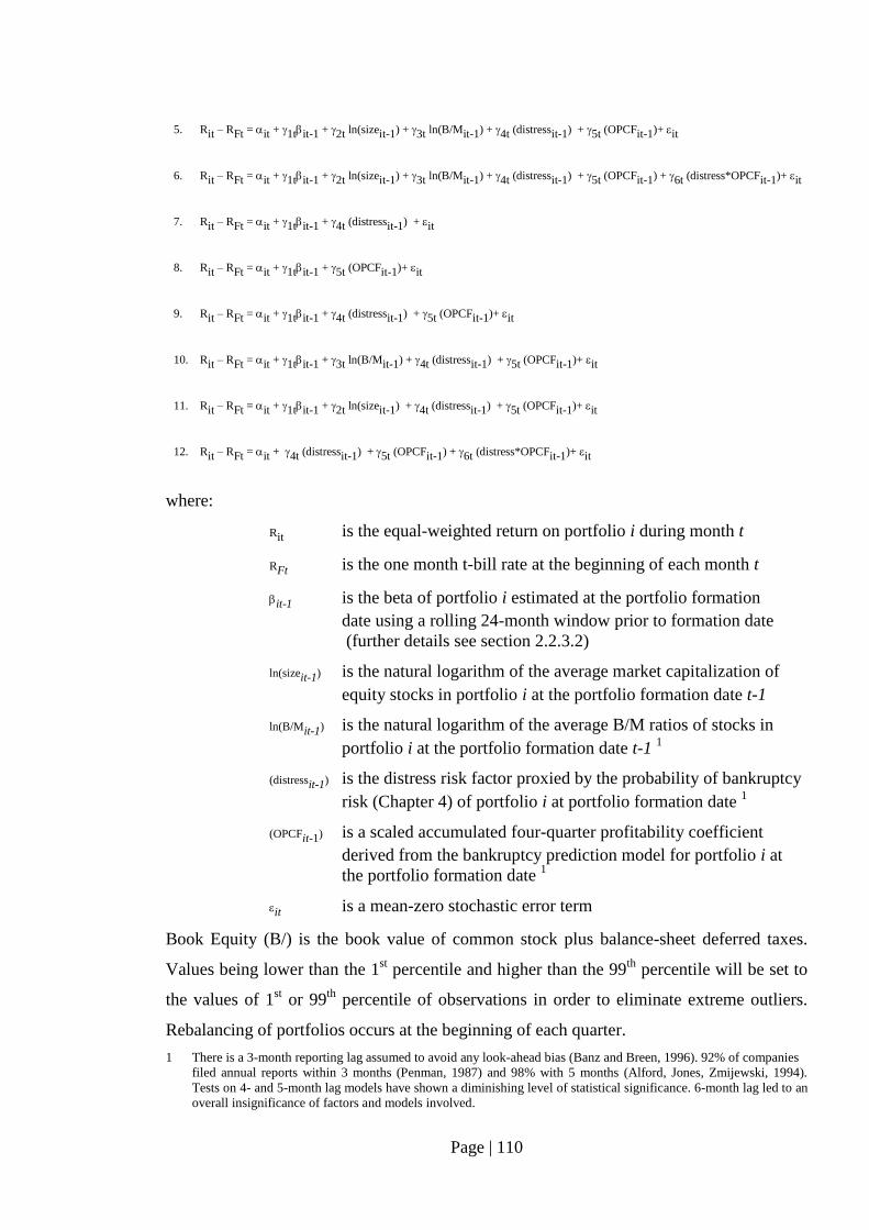
Page | 110
5. Rit – RFt = it + 1tit-1 + 2t ln(sizeit-1) + 3t ln(B/Mit-1) + 4t (distressit-1) + 5t (OPCFit-1)+ it
6. Rit – RFt = it + 1tit-1 + 2t ln(sizeit-1) + 3t ln(B/Mit-1) + 4t (distressit-1) + 5t (OPCFit-1) + 6t (distress*OPCFit-1)+ it
7. Rit – RFt = it + 1tit-1 + 4t (distressit-1) + it
8. Rit – RFt = it + 1tit-1 + 5t (OPCFit-1)+ it
9. Rit – RFt = it + 1tit-1 + 4t (distressit-1) + 5t (OPCFit-1)+ it
10. Rit – RFt = it + 1tit-1 + 3t ln(B/Mit-1) + 4t (distressit-1) + 5t (OPCFit-1)+ it
11. Rit – RFt = it + 1tit-1 + 2t ln(sizeit-1) + 4t (distressit-1) + 5t (OPCFit-1)+ it
12. Rit – RFt = it + 4t (distressit-1) + 5t (OPCFit-1) + 6t (distress*OPCFit-1)+ it
where:
Rit is the equal-weighted return on portfolio i during month t
RFt is the one month t-bill rate at the beginning of each month t
it-1 is the beta of portfolio i estimated at the portfolio formation
date using a rolling 24-month window prior to formation date
(further details see section 2.2.3.2)
ln(sizeit-1) is the natural logarithm of the average market capitalization of
equity stocks in portfolio i at the portfolio formation date t-1
ln(B/Mit-1) is the natural logarithm of the average B/M ratios of stocks in
portfolio i at the portfolio formation date t-1 1
(distressit-1) is the distress risk factor proxied by the probability of bankruptcy
risk (Chapter 4) of portfolio i at portfolio formation date 1
(OPCFit-1) is a scaled accumulated four-quarter profitability coefficient
derived from the bankruptcy prediction model for portfolio i at
the portfolio formation date 1
it is a mean-zero stochastic error term
Book Equity (B/) is the book value of common stock plus balance-sheet deferred taxes.
Values being lower than the 1st percentile and higher than the 99
th percentile will be set to
the values of 1st or 99
th percentile of observations in order to eliminate extreme outliers.
Rebalancing of portfolios occurs at the beginning of each quarter.
1 There is a 3-month reporting lag assumed to avoid any look-ahead bias (Banz and Breen, 1996). 92% of companies
filed annual reports within 3 months (Penman, 1987) and 98% with 5 months (Alford, Jones, Zmijewski, 1994).
Tests on 4- and 5-month lag models have shown a diminishing level of statistical significance. 6-month lag led to an
overall insignificance of factors and models involved.
Page | 111
5.6 Results: Empirical Analysis
5.6.1 Results Descriptive Statistics
The main objective of the descriptive statistics is to test the hypotheses in full and/or in
part especially related to H2Aa), H2Ab) and H2Ac) as outlined in section 3.3. In addition, it
describes the mean values of different characteristics related to stock returns by various
portfolio sorts as outlined in section 5.5.2. The statistical significance of factors describing
these returns is documented by the Fama and MacBeth (1973) t-statistics and is covered in
sections 5.5.4 and 5.6.3.
A first overview is provided by a distress risk deciles sorted portfolio (Table 5.6.1.1 and
Figures 5.6.1.1 to 5.6.1.6). The monthly average excess returns slightly decrease from 1.4%
to 1.3% over the first five distress risk deciles but then increase up to 1.7% at 8th
decile.
The 8th
distress decile has a mean distress risk probability p of 0.50 as shown in panel E. A
bankrupt stock is by definition rather found with a probability of failure larger than p 0.50
hence at the 9th
and 10th
deciles. These two deciles show a strong shortfall in mean excess
returns with 1.1% and 0.9% respectively when comparing to the group of non-bankrupt
securities in the 8th
distress risk decile, but also when benchmarking with the lowest
distress risk portfolios. The excess return analysis as illustrated by figure 5.6.1.1 indicates
that distressed stocks underperform on average the non-distressed ones.
The apparent average underperformance of highly distressed stocks may eventually be
described by other characteristics than by the distress risk factor itself. Figure 5.6.1.6
shows that on average, companies having a distress risk factor of equal or less p 0.50 (up to
the 8th
decile) have a positive OPCF (scaled operating cash flow before interest and taxes
paid) while distressed companies at the 9th
and 10th
deciles generate a negative OPCF. It
appears that the current profitability strength measured by OPCF could be an important
factor in describing stock returns not only for highly distressed, but stocks in general. In
short, firms with a relative distress risk higher than p 0.50 generate on average negative
operating cash flows. Figure 5.6.133 shows that stocks generating positive operating cash
flows (OPCF) maintain a positive risk-return relationship also at highest distress level
whereas the group of negative OPCF earn low average returns at comparable distress risk
levels. This suggests that the underperformance of highly distressed stocks may be
Page | 112
explained by the conditionality between the continuous distress risk and the current
profitability strength factor proxied by OPCF.
In a two-way intersecting OPCF-Distress set of portfolios (Table 5.6.1.2, Figures 5.6.1.7 to
5.6.1.10 – all in Appendix A), the descriptive statistics indicate that distressed companies
of the 5th
distress risk quintile earn lower returns than those in the 4th
quintile unless they
are highly profitable as shown by Figure 5.6.1.7 (Appendix A). This is also confirmed
when distress risk deciles sorted by positive and negative OPCF portfolios (Figure
5.6.1.33).
Figure 5.6.1.29 of three-way sorted Size - B/M - Distress portfolios reveal that only big
companies with high B/M maintain the positive distress risk premium up to the 5th
quintile
of distress risk as these companies generate on average still positive operating cash flows
throughout all distress risk levels. (Table 5.6.1.6, Figure 5.6.1.32). Two-way sorted B/M -
Distress risk portfolios (Table 5.6.1.4, Appendix A) confirm the above findings where
distress risk is positively priced up to the 4th
distress risk quintile with an average p of 0.49,
but it then diminishes once stocks are distressed and unprofitable. Figure 5.6.1.29 sums it
up. Big Size – high B/M companies in the computer and electronics industry earn lower
returns compared to other portfolios, but appear to maintain a positive continuous distress
risk premium up to the highest distress risk quintile as result of still producing positive
cash flows or current profitability strength.
So, if the financial distress factor hypothesis of Fama and French (1992) holds and my
distress risk factor as used in this study is valid I then should expect to see the average B/M
factor increasing and the average Size factor decreasing along the low to high distress risk
quintiles or deciles axes. The distress deciles sorted portfolios, however, give a different
picture. Table 5.6.1.1, Panel D, and Figure 5.6.1.4 show that low and high distressed stocks
share a similar level of mean ln(B/M) values. The ln(B/M) values increase from the lowest
to the 5th
distress decile but then drop again rather than analogously increase with distress
risk levels. It depicts an inverted u-shape and confirms Dichev’s (1998) finding. As a
consequence, portfolios ranked by B/M quartiles would cause low and high distressed
stocks to be combined in the first B/M quartile since they share similarly low ln(B/M)
values. Dichev (1998) concludes that highly distressed stocks have a low rather than high
Page | 113
B/M and earn low returns which is consistent with my finding as reflected by Figures
5.6.1.1 and 5.6.1.4. Table 5.6.1.5 in Appendix A illustrates the descriptive statistics of 16
independently sorted Size - B/M portfolios and confirm Dichev’s (1998) finding in so far
that the distress risk probability for low B/M stocks is found at p 0.42, going down to p
0.34 and then upwards again to p 0.35 and p 0.39 for the high B/M portfolio. This u-shape
of probability of failure risk distribution along the B/M quartiles axis (Figure 5.6.1.27,
Appendix A) seems to confirm that both stocks with high and low distress risks are
averaged in the low B/M portfolio. However, there is also a different result for the Size
factor which does expectedly decrease along the axis of distress risk deciles (Figure 5.6.1.3)
thus eventually mirrors distress risk. Further tests on these two factors will be conducted in
sections 5.5.3 and 5.5.4.
Other results
Besides the results above, the descriptive statistics also provides monthly average excess
return information on a portfolio by portfolio basis. The highest excess returns are
achieved by a high OPCF – High Distress portfolio with a monthly average of 2.8% (Table
5.6.1.2, Appendix A). This is also in line with the above findings. The first is that firms
with a higher profitability achieve higher returns while loss making companies which are
proxied by negative operating cash flows before interest and taxes paid earn on average
lower returns (earnings levels – returns relationship proposition, section 2.3). The second
in parallel is that it appears that distress risk is positively priced thus highly distressed
stocks earn a higher premium than non-distressed stocks following a risk based rational
pricing proposition. As result, the cross-sectional regressions tests of these two factors may
occur jointly given the potential conditionality between these two factors. Both factors,
distress and OPCF are tested for statistical significance in a number of multivariate settings
(section 5.6.3).
Figure 5.6.1.25 indicates that growth stocks may actually earn higher returns than value
stocks which is specific to this industry and eventually to the period tested. On average,
low B/M stock earned a monthly excess return of 2% whereas high B/M only 0.8% for the
1990 – 2006 period (see comments regarding periodically changing signs of B/M and size
factors in section 2.2.3.3).
Page | 114
Another interesting finding is that the average beta is quite linearly increasing along the
Distress risk deciles and quintiles axes (Figures 5.6.1.2 and other figures in Appendix A).
This somewhat confirms that the distress risk probabilities derived from the bankruptcy
prediction model appear to measure the underlying risk of failure with a right tendency.
However both, the market factor and the distress risk factor as univariates may not be able
to explain the distressed stocks’ average underperformance in a linear fashion.
Given the results above it appears that H2Aa) cannot be rejected. Additional cross-sectional
regressions need to be performed to confirm the statistical significance of the above results
(sections 5.5.4 and 5.6.3). The additional finding that the B/M factor is following an
inverted u-shape along the low to high distress risk axis is in contrast with the distress
factor proposition made by Fama and French (1992). It indicates that H2Ab) cannot be
rejected. However, the Size factor appears to mirror somewhat the distress risk factor, but
it needs to be confirmed by correlation and cross-sectional regression tests. A final
conclusion for this hypothesis related to the Fama-French distress factor proposition has to
be made in connection with the test results in sections 5.6.2 and 5.6.3.
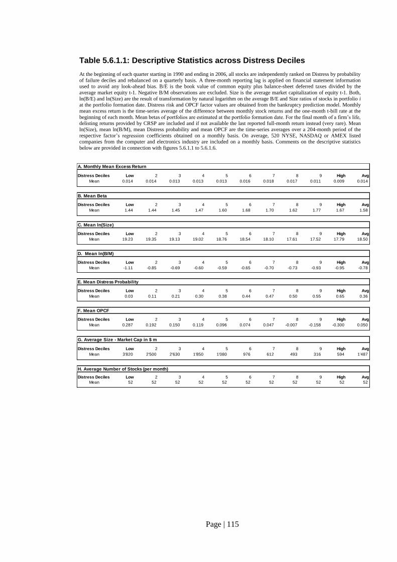
Page | 115
Table 5.6.1.1: Descriptive Statistics across Distress Deciles At the beginning of each quarter starting in 1990 and ending in 2006, all stocks are independently ranked on Distress by probability
of failure deciles and rebalanced on a quarterly basis. A three-month reporting lag is applied on financial statement information used to avoid any look-ahead bias. B/E is the book value of common equity plus balance-sheet deferred taxes divided by the
average market equity t-1. Negative B/M observations are excluded. Size is the average market capitalization of equity t-1. Both,
ln(B/E) and ln(Size) are the result of transformation by natural logarithm on the average B/E and Size ratios of stocks in portfolio i at the portfolio formation date. Distress risk and OPCF factor values are obtained from the bankruptcy prediction model. Monthly
mean excess return is the time-series average of the difference between monthly stock returns and the one-month t-bill rate at the
beginning of each month. Mean betas of portfolios are estimated at the portfolio formation date. For the final month of a firm’s life, delisting returns provided by CRSP are included and if not available the last reported full-month return instead (very rare). Mean
ln(Size), mean ln(B/M), mean Distress probability and mean OPCF are the time-series averages over a 204-month period of the
respective factor’s regression coefficients obtained on a monthly basis. On average, 520 NYSE, NASDAQ or AMEX listed companies from the computer and electronics industry are included on a monthly basis. Comments on the descriptive statistics
below are provided in connection with figures 5.6.1.1 to 5.6.1.6.
A. Monthly Mean Excess Return
Distress Deciles Low 2 3 4 5 6 7 8 9 High Avg
Mean 0.014 0.014 0.013 0.013 0.013 0.016 0.018 0.017 0.011 0.009 0.014
B. Mean Beta
Distress Deciles Low 2 3 4 5 6 7 8 9 High Avg
Mean 1.44 1.44 1.45 1.47 1.60 1.68 1.70 1.62 1.77 1.67 1.58
C. Mean ln(Size)
Distress Deciles Low 2 3 4 5 6 7 8 9 High Avg
Mean 19.23 19.35 19.13 19.02 18.76 18.54 18.10 17.61 17.52 17.79 18.50
D. Mean ln(B/M)
Distress Deciles Low 2 3 4 5 6 7 8 9 High Avg
Mean -1.11 -0.85 -0.69 -0.60 -0.59 -0.65 -0.70 -0.73 -0.93 -0.95 -0.78
E. Mean Distress Probability
Distress Deciles Low 2 3 4 5 6 7 8 9 High Avg
Mean 0.03 0.11 0.21 0.30 0.38 0.44 0.47 0.50 0.55 0.65 0.36
F. Mean OPCF
Distress Deciles Low 2 3 4 5 6 7 8 9 High Avg
Mean 0.287 0.192 0.150 0.119 0.096 0.074 0.047 -0.007 -0.158 -0.300 0.050
G. Average Size - Market Cap in $ m
Distress Deciles Low 2 3 4 5 6 7 8 9 High Avg
Mean 3'820 2'500 2'630 1'850 1'080 976 612 493 316 594 1'487
H. Average Number of Stocks (per month)
Distress Deciles Low 2 3 4 5 6 7 8 9 High Avg
Mean 52 52 52 52 52 52 52 52 52 52 52
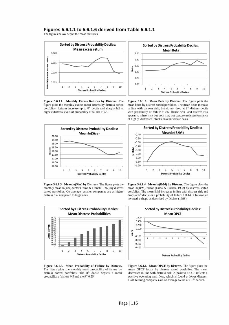
Page | 116
Figures 5.6.1.1 to 5.6.1.6 derived from Table 5.6.1.1 The figures below depict the mean statistics
Figure 5.6.1.1. Monthly Excess Returns by Distress. The
figure plots the monthly excess mean returns by distress sorted portfolios. Returns increase up to 8th decile and sharply fall at
highest distress levels of probability of failure > 0.5.
Figure 5.6.1.2. Mean Beta by Distress. The figure plots the
mean betas by distress sorted portfolios. The mean betas increase in line with distress risk, but do not drop at 9th distress decile
with probability of failure > 0.5. Hence beta and distress risk
appear to mirror risk but both may not capture underperformance of highly distressed stocks on a univariate basis.
Figure 5.6.1.3. Mean ln(Size) by Distress. The figure plots the
monthly mean ln(size) factor (Fama & French, 1992) by distress
sorted portfolios. On average, smaller companies are at higher distress risk compared to large ones.
Figure 5.6.1.4. Mean ln(B/M) by Distress. The figure plots the
mean ln(B/M) factor (Fama & French, 1992) by distress sorted
portfolios. The mean B/M increases in line with distress risk and drops at 6th decile or a probability of failure > 0.44. It follows an
inverted u-shape as described by Dichev (1998).
Figure 5.6.1.5. Mean Probability of Failure by Distress.
The figure plots the monthly mean probability of failure by
distress sorted portfolios. The 8th decile depicts a mean
probability of failure 0.5 and the 9th 0.55.
Figure 5.6.1.6. Mean OPCF by Distress. The figure plots the
mean OPCF factor by distress sorted portfolios. The mean
decreases in line with distress risk. A positive OPCF reflects a
positive operating cash flow, which is found at lower distress. Cash burning companies are on average found at > 8th deciles.
0.005
0.010
0.015
0.020
1 2 3 4 5 6 7 8 9 10Mo
nth
ly m
ea
n e
xce
ss r
etu
rn
Distress Probability Deciles
Sorted by Distress Probability Deciles: Mean excess return
1.00
1.20
1.40
1.60
1.80
2.00
1 2 3 4 5 6 7 8 9 10
Be
ta
Distress Probability Deciles
Sorted by Distress Probability Deciles: Mean Beta
16.00
16.50
17.00
17.50
18.00
18.50
19.00
19.50
20.00
1 2 3 4 5 6 7 8 9 10
ln(S
ize
)
Distress Probability Deciles
Sorted by Distress Probability Deciles: Mean ln(Size)
-1.20
-1.10
-1.00
-0.90
-0.80
-0.70
-0.60
-0.50
-0.40
1 2 3 4 5 6 7 8 9 10
ln(B
/M)
Distress Probability Deciles
Sorted by Distress Probability Deciles: Mean ln(B/M)
-0.05 0.10 0.15 0.20 0.25 0.30 0.35 0.40 0.45 0.50 0.55 0.60 0.65 0.70
1 2 3 4 5 6 7 8 9 10
Dis
tre
ss P
rob
Distress Probability Deciles
Sorted by Distress Probability Deciles: Mean Distress Probabilities
-0.400
-0.300
-0.200
-0.100
-
0.100
0.200
0.300
0.400
1 2 3 4 5 6 7 8 9 10
OP
CF
Distress Probability Deciles
Sorted by Distress Probability Deciles: Mean OPCF
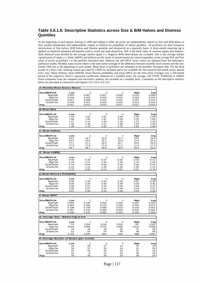
Page | 117
Table 5.6.1.6: Descriptive Statistics across Size & B/M Halves and Distress Quintiles At the beginning of each quarter starting in 1990 and ending in 2006, all stocks are independently ranked on Size and B/M halves at
their median breakpoints and independently ranked on Distress by probability of failure quintiles. 20 portfolios are then formed at intersections of Size halves, B/M halves and Distress quintiles and rebalanced on a quarterly basis. A three-month reporting lag is
applied on financial statement information used to avoid any look-ahead bias. B/E is the book value of common equity plus balance-
sheet deferred taxes divided by the average market equity t-1. Negative B/M observations are excluded. Size is the average market capitalization of equity t-1. Both, ln(B/E) and ln(Size) are the result of transformation by natural logarithm on the average B/E and Size
ratios of stocks in portfolio i at the portfolio formation date. Distress risk and OPCF factor values are obtained from the bankruptcy
prediction model. Monthly mean excess return is the time-series average of the difference between monthly stock returns and the one-month t-bill rate at the beginning of each month. Mean betas of portfolios are estimated at the portfolio formation date. For the final
month of a firm’s life, delisting returns provided by CRSP are included and if not available the last reported full-month return instead
(very rare). Mean ln(Size), mean ln(B/M), mean Distress probability and mean OPCF are the time-series averages over a 204-month period of the respective factor’s regression coefficients obtained on a monthly basis. On average, 520 NYSE, NASDAQ or AMEX
listed companies from the computer and electronics industry are included on a monthly basis. Comments on the descriptive statistics
below are provided in connection with figures 5.6.1.29 to 5.6.1.32.
A. Monthly Mean Excess Return
Size/BM/Prob Low 2 3 4 High Avg
Big/High 0.005 0.007 0.007 0.009 0.013 0.008
Big/Low 0.018 0.019 0.020 0.022 0.015 0.019
Small/High 0.007 0.008 0.012 0.016 0.007 0.010
Small/Low 0.019 0.021 0.018 0.022 0.011 0.018
Avg 0.012 0.014 0.014 0.017 0.012 0.014
B. Mean Beta
Size/BM/Prob Low 2 3 4 High Avg
Big/High 1.55 1.61 1.87 2.08 2.04 1.83
Big/Low 1.56 1.65 1.91 2.09 2.02 1.85
Small/High 1.17 1.14 1.33 1.42 1.57 1.33
Small/Low 1.16 1.30 1.37 1.46 1.64 1.39
Avg 1.36 1.43 1.62 1.76 1.82 1.60
C. Mean ln(Size)
Size/BM/Prob Low 2 3 4 High Avg
Big/High 19.5 19.7 19.8 19.7 19.5 19.6
Big/Low 20.5 20.6 20.1 19.6 19.5 20.1
Small/High 17.1 17.1 16.9 16.7 16.6 16.9
Small/Low 17.5 17.6 17.3 17.1 17.2 17.3
Avg 18.7 18.7 18.6 18.3 18.2 18.5
D. Mean ln(B/M)
Size/BM/Prob Low 2 3 4 High Avg
Big/High -0.40 -0.33 -0.27 -0.28 -0.29 -0.31
Big/Low -1.43 -1.27 -1.33 -1.53 -1.76 -1.46
Small/High -0.19 -0.04 -0.00 0.00 0.00 -0.04
Small/Low -1.13 -1.12 -1.28 -1.42 -1.60 -1.31
Avg -0.79 -0.69 -0.72 -0.81 -0.91 -0.78
E. Mean Distress Probability
Size/BM/Prob Low 2 3 4 High Avg
Big/High 0.09 0.26 0.40 0.48 0.57 0.36
Big/Low 0.06 0.24 0.40 0.48 0.59 0.35
Small/High 0.08 0.27 0.42 0.49 0.58 0.37
Small/Low 0.05 0.27 0.42 0.49 0.63 0.37
Avg 0.07 0.26 0.41 0.48 0.59 0.36
F. Mean OPCF
Size/BM/Prob Low 2 3 4 High Avg
Big/High 0.200 0.130 0.091 0.046 -0.001 0.093
Big/Low 0.263 0.164 0.110 0.035 -0.202 0.074
Small/High 0.198 0.109 0.068 0.019 -0.135 0.052
Small/Low 0.257 0.122 0.059 -0.009 -0.432 -0.001
Avg 0.230 0.131 0.082 0.023 -0.193 0.055
G. Average Size - Market Cap in $ m
Size/BM/Prob Low 2 3 4 High Avg
Big/High 779 1'320 1'240 1'020 767 1'025
Big/Low 6'010 5'090 2'270 1'460 1'510 3'268
Small/High 43 45 39 35 31 39
Small/Low 61 64 54 48 46 55
Avg 1'723 1'630 901 641 588 1'097
H. Average Number of Stocks (per month)
Size/BM/Prob Low 2 3 4 High Avg
Big/High 16 28 27 14 10 19
Big/Low 55 37 30 24 21 33
Small/High 22 31 35 43 37 34
Small/Low 12 8 13 24 36 19
Avg 26 26 26 26 26 26
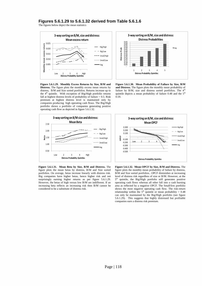
Page | 118
Figures 5.6.1.29 to 5.6.1.32 derived from Table 5.6.1.6 The figures below depict the mean statistics
Figure 5.6.1.29. Monthly Excess Returns by Size, B/M and
Distress. The figure plots the monthly excess mean returns by distress, B/M and Size sorted portfolios. Returns increase up to
the 4th quintile. With exception of Big/High portfolio returns
fall at highest distress levels of probability of failure > 0.5. Risk premium at highest distress level is maintained only by
companies producing high operating cash flows. The Big/High
portfolio shows a portfolio of companies generating positive operating cash flow as depicted in figure 5.6.1.32.
Figure 5.6.1.30. Mean Probability of Failure by Size, B/M
and Distress. The figure plots the monthly mean probability of failure by B/M, size and distress sorted portfolios. The 4th
quintile depicts a mean probability of failure 0.48 and the 5th
0.59.
Figure 5.6.1.31. Mean Beta by Size, B/M and Distress. The figure plots the mean betas by distress, B/M and Size sorted
portfolios. On average, betas increase linearly with distress risk.
Big companies have higher betas, hence higher risk and not surprisingly earning higher returns as per figure 5.6.1.29.
However, the betas of high versus low B/M are indifferent. If an
increasing beta reflects an increasing risk then B/M cannot be considered to be a substitute of distress risk.
Figure 5.6.1.32. Mean OPCF by Size, B/M and Distress. The figure plots the monthly mean probability of failure by distress,
B/M and Size sorted portfolios.. OPCF diminishes at increasing
level of distress risk regardless of size or B/M. However, at the 5th quintile, the Big/High portfolio still generates positive
operating cash flows whereas all other fall into a cash burning
area as reflected by a negative OPCF. The Small/low portfolio shows the most negative operating cash flow. The risk-return
relationship within the 5th quintile or mean probability > 0.48
can only be maintained by the Big/High portfolio (see figure 5.6.1.29). This suggests that highly distressed but profitable
companies earn a distress risk premium.
-
0.005
0.010
0.015
0.020
0.025
Low 2 3 4 High
Mo
nth
ly m
ea
n e
xce
ss r
etu
rn
Distress Probability Quintiles
3-way sorting on B/M, size and distress: Mean excess return
Big/High
Big/Low
Small/High
Small/Low
Avg-
0.05 0.10 0.15 0.20 0.25 0.30 0.35 0.40 0.45 0.50 0.55 0.60 0.65
1 2 3 4 5
Dis
tre
ss P
rob
Distress Probability Quintiles
3-way sorting on B/M, size and distress: Distress Probabilities
Avg
0.50
1.00
1.50
2.00
2.50
Low 2 3 4 High
Be
ta
Distress Probability Quintiles
3-way sorting on B/M size and distress: Mean Beta
Big/High
Big/Low
Small/High
Small/Low
Avg
-0.500
-0.400
-0.300
-0.200
-0.100
-
0.100
0.200
0.300
Low 2 3 4 High
OP
CF
Distress Probability Quintiles
3-way sorting on B/M, size and distress: Mean OPCF
Big/High
Big/Low
Small/High
Small/Low
Avg
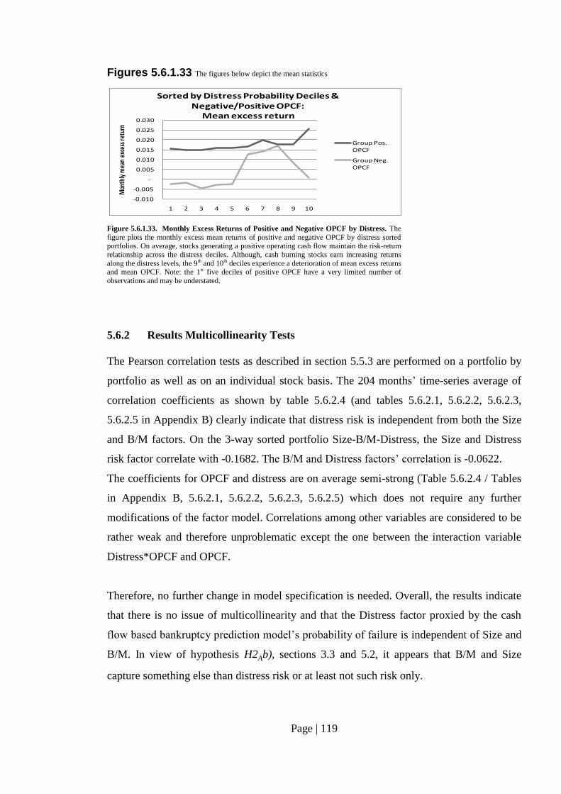
Page | 119
Figures 5.6.1.33 The figures below depict the mean statistics
Figure 5.6.1.33. Monthly Excess Returns of Positive and Negative OPCF by Distress. The
figure plots the monthly excess mean returns of positive and negative OPCF by distress sorted portfolios. On average, stocks generating a positive operating cash flow maintain the risk-return
relationship across the distress deciles. Although, cash burning stocks earn increasing returns
along the distress levels, the 9th and 10th deciles experience a deterioration of mean excess returns and mean OPCF. Note: the 1st five deciles of positive OPCF have a very limited number of
observations and may be understated.
5.6.2 Results Multicollinearity Tests
The Pearson correlation tests as described in section 5.5.3 are performed on a portfolio by
portfolio as well as on an individual stock basis. The 204 months’ time-series average of
correlation coefficients as shown by table 5.6.2.4 (and tables 5.6.2.1, 5.6.2.2, 5.6.2.3,
5.6.2.5 in Appendix B) clearly indicate that distress risk is independent from both the Size
and B/M factors. On the 3-way sorted portfolio Size-B/M-Distress, the Size and Distress
risk factor correlate with -0.1682. The B/M and Distress factors’ correlation is -0.0622.
The coefficients for OPCF and distress are on average semi-strong (Table 5.6.2.4 / Tables
in Appendix B, 5.6.2.1, 5.6.2.2, 5.6.2.3, 5.6.2.5) which does not require any further
modifications of the factor model. Correlations among other variables are considered to be
rather weak and therefore unproblematic except the one between the interaction variable
Distress*OPCF and OPCF.
Therefore, no further change in model specification is needed. Overall, the results indicate
that there is no issue of multicollinearity and that the Distress factor proxied by the cash
flow based bankruptcy prediction model’s probability of failure is independent of Size and
B/M. In view of hypothesis H2Ab), sections 3.3 and 5.2, it appears that B/M and Size
capture something else than distress risk or at least not such risk only.
-0.010
-0.005
-
0.005
0.010
0.015
0.020
0.025
0.030
1 2 3 4 5 6 7 8 9 10
Mon
thly
mea
n ex
cess
retu
rn
Sorted by Distress Probability Deciles & Negative/Positive OPCF:
Mean excess return
Group Pos. OPCF
Group Neg. OPCF
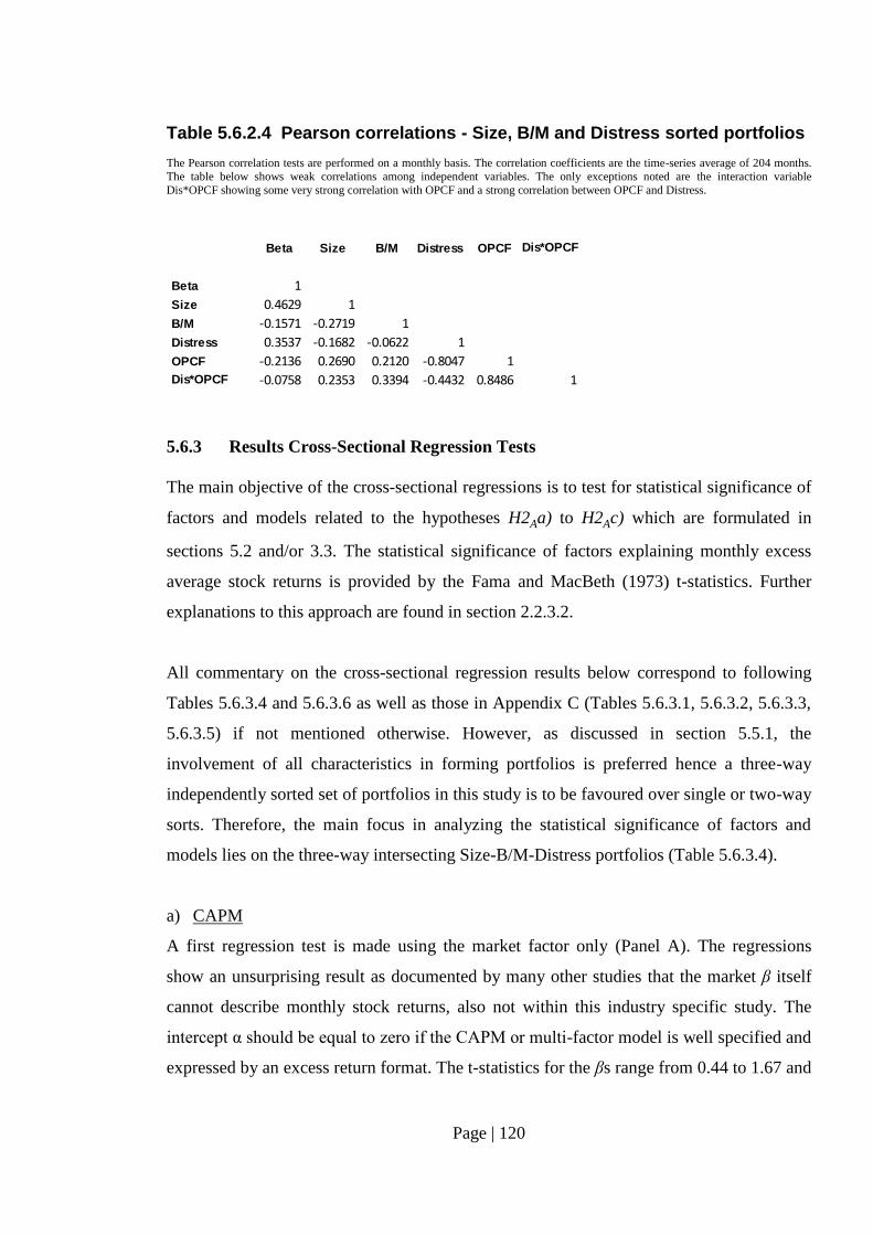
Page | 120
Table 5.6.2.4 Pearson correlations - Size, B/M and Distress sorted portfolios The Pearson correlation tests are performed on a monthly basis. The correlation coefficients are the time-series average of 204 months.
The table below shows weak correlations among independent variables. The only exceptions noted are the interaction variable
Dis*OPCF showing some very strong correlation with OPCF and a strong correlation between OPCF and Distress.
5.6.3 Results Cross-Sectional Regression Tests
The main objective of the cross-sectional regressions is to test for statistical significance of
factors and models related to the hypotheses H2Aa) to H2Ac) which are formulated in
sections 5.2 and/or 3.3. The statistical significance of factors explaining monthly excess
average stock returns is provided by the Fama and MacBeth (1973) t-statistics. Further
explanations to this approach are found in section 2.2.3.2.
All commentary on the cross-sectional regression results below correspond to following
Tables 5.6.3.4 and 5.6.3.6 as well as those in Appendix C (Tables 5.6.3.1, 5.6.3.2, 5.6.3.3,
5.6.3.5) if not mentioned otherwise. However, as discussed in section 5.5.1, the
involvement of all characteristics in forming portfolios is preferred hence a three-way
independently sorted set of portfolios in this study is to be favoured over single or two-way
sorts. Therefore, the main focus in analyzing the statistical significance of factors and
models lies on the three-way intersecting Size-B/M-Distress portfolios (Table 5.6.3.4).
a) CAPM
A first regression test is made using the market factor only (Panel A). The regressions
show an unsurprising result as documented by many other studies that the market β itself
cannot describe monthly stock returns, also not within this industry specific study. The
intercept α should be equal to zero if the CAPM or multi-factor model is well specified and
expressed by an excess return format. The t-statistics for the βs range from 0.44 to 1.67 and
Beta Size B/M Distress OPCF Dis*OPCF
Beta 1
Size 0.4629 1
B/M -0.1571 -0.2719 1
Distress 0.3537 -0.1682 -0.0622 1
OPCF -0.2136 0.2690 0.2120 -0.8047 1
Dis*OPCF -0.0758 0.2353 0.3394 -0.4432 0.8486 1
Page | 121
thus they are not significantly different from zero. The αs, which are expected to be
economically and statistically indifferent from zero, are higher than the βs and in most
cases significantly different from zero with t-statistics found in the range of 1.14 to 2.39.
Given the above result, it looks like β is dead or at least flat.
b) 3-Factor Fama-French (1992)
The second specification tested is the Fama and French (1992) model which includes
factors for Size and B/M (Panel B). This model also provides the basis for measuring the
incremental impact of added factors such as relative distress risk and current profitability
strength (OPCF). The three-factor model regression reveals that B/M has some strong
explanatory power in almost all sets of portfolios and models with the exception of
portfolios sorted without the B/M characteristics (Table 5.6.3.1, 5.6.3.2 in Appendix C).
However, the average slope of B/M is negative, a contrary outcome to other studies (see
section 5.6.1), but consistent with the descriptive statistics’ results reported by Figure
5.6.1.25 in Appendix A. In a set of three-way intersecting portfolios with Size (2), B/M (2)
and Distress (5) characteristics (Table 5.6.3.4) the slope for B/M is -0.0065 with a highly
significant t-statistics of -3.90. Similar values are found with other portfolio formations as
long as the B/M characteristics sort is included. Hence, growth stocks earn a higher
premium than value stocks in the US computer and electronics industry. Loughran (1997)
shows in his study that the B/M factor had changing signs over several periods and that it
was negative for the years 1985 to 1995. This anomaly could be explained by the fact that
the computer and electronics industry was growth oriented over this period of rapid
technological advancement. Investors may have awarded high multiples relative to the
book equity for these industry-specific companies by anticipating substantially higher
future sales and earnings compared to the prevalent fundamentals given at the time of
investment.
The other two factors, Size and β are both insignificant in describing stock returns (see
section 2.2.3.3). The βs show in some portfolios (Table 5.6.3.2, Appendix C) even a
negative slope. This finding is consistent with Fama and French (1992), Lakonishok and
Shapiro (1986) and others. The Size factor is insignificant in both univariate and
multivariate regression tests. This finding is not of surprise as the size effect has been
found to be weak or even nonexistent starting in the 1980s (Dichev, 1998).
Page | 122
The third group of specifications (Panel C) includes various multi-factor model
combinations. The focus lies on the Distress risk and current profitability strength (OPCF)
factors which are tested in different settings as discussed below.
c) Distress Risk Factor
Model 3) reflects the Fama and French (1992) three-factor model augmented by the
Distress factor only. In all set of portfolios except Table 6.5.3.5 (Appendix C), the distress
factor premium without the profitability factor cannot explain stock returns significantly.
The same is true when the CAPM is extended by the distress factor as shown with model
7). The distress risk factor cannot grasp monthly excess stock returns linearly as concluded
in section 5.6.1 (descriptive statistics) as it appears that non-distressed stocks are rewarded
on average with a positive distress risk premium depending on profitability strength, but
that distressed stocks as a separate group on average underperform. Nevertheless despite
its insignificance as a univariate, the positive slope of distress can be interpreted to be a
premium reward as expected by a risk based rational pricing proposition (section 3.1).
d) OPCF Factor as proxy for Profitability Levels
The current profitability strength factor which is proxied by the OPCF coefficient shows
some stronger explanatory power when used as augmentation of the Fama-French three-
factor model or the CAPM. Model 4) shows again the Fama and French (1992)
specification augmented by the OPCF factor is significant at 0.10 level in a three-way-
sorted portfolio (Table 5.6.3.4). In particular, this factor is highly significant in OPCF
sorted portfolios (Table 5.6.3.1, Appendix C) with t-statistics of – 3.89. The positive slope
of OPCF can be interpreted to be a premium reward as expected by the earnings levels to
return relationship proposition (section 3.1). Model 8) is the market model extended by the
OPCF factor only confirming the above results.
e) Distress and OPCF in a Joint Setting and Conditionality between the two Factors
As discussed under c) a stand-alone relative distress risk factor cannot describe stock
returns which is also not a surprise when looking into the descriptive statistics (Figure
5.6.1.1, 5.6.1.29). However, the descriptive statistics (Figure 5.6.1.33) also reveal that the
Page | 123
distress risk factor conditional on profitability (OPCF) may price a positive distress risk
premium.
Based on the research question and the hypotheses set in section 3.3, various models that
include distress risk and profitability (OPCF) factors are tested jointly in a multivariate
setting. The focus lies on model 10) derived from two theoretical propositions discussed in
section 3.1 as well as model 12) which should provide evidence of the conditionality
between distress risk and profitability levels (OPCF).
Nevertheless, the first specification discussed is model 5) which is a five-factor model
made of Fama-French’s (1992) three-factor plus distress risk and profitability (OPCF). In
all sets of portfolios the five-factor model has significantly improved the explanatory
power (adj R2) over the Fama-French’s three-factor model. In addition, the Distress risk
and OPCF factors are in most of the cases highly significant at 0.01 level and do help
increasing the t-statistics of the B/M and Size factors too. An increased distress risk
provides a positive distress risk premium on a continuous basis in a joint setting with
profitability (OPCF) hence it follows a risk based rational pricing proposition as discussed
in section 3.1. The profitability (OPCF) factor also shows a positive slope in a joint setting
with distress risk and confirms the positive profitability (earnings) levels to return
relationship also discussed in section 3.1. Comparing model 5) and 10) with model 2) also
indicates that the inclusion of the distress risk and profitability (OPCF) factors improves
the t-statistics of both the B/M and size factors. Hence, the Distress risk and OPCF factors
are not subsumed by the size or B/M factors. The improvement of t-statistics of B/M and
Size by adding the distress risk and OPCF factors confirm the findings of section 5.6.2
where B/M and Size is found to capture something other than distress risk. If such risk was
proxied by B/M or Size, one should have expected that either of these variables to become
less significant or even insignificant in explaining returns. This also confirms the findings
as described in section 5.6.1 where B/M illustrates an inverted u-shape along the distress
risk deciles axis.
Overall, the B/M factor is highly significant at 0.01 level in any of the model specifications
tested whereas Size and β are insignificant with less than one standard error from zero. In
the Fama-French (1992) three-factor model 3), the B/M factor shows a negative slope of -
0.0065 with a t-statistics of -3.90 which means that growth stocks earned on average a
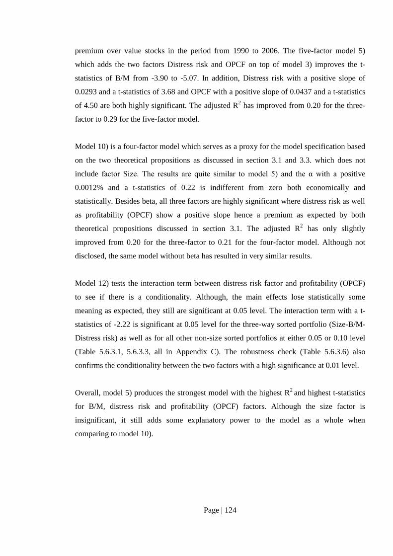
Page | 124
premium over value stocks in the period from 1990 to 2006. The five-factor model 5)
which adds the two factors Distress risk and OPCF on top of model 3) improves the t-
statistics of B/M from -3.90 to -5.07. In addition, Distress risk with a positive slope of
0.0293 and a t-statistics of 3.68 and OPCF with a positive slope of 0.0437 and a t-statistics
of 4.50 are both highly significant. The adjusted R2 has improved from 0.20 for the three-
factor to 0.29 for the five-factor model.
Model 10) is a four-factor model which serves as a proxy for the model specification based
on the two theoretical propositions as discussed in section 3.1 and 3.3. which does not
include factor Size. The results are quite similar to model 5) and the α with a positive
0.0012% and a t-statistics of 0.22 is indifferent from zero both economically and
statistically. Besides beta, all three factors are highly significant where distress risk as well
as profitability (OPCF) show a positive slope hence a premium as expected by both
theoretical propositions discussed in section 3.1. The adjusted R2 has only slightly
improved from 0.20 for the three-factor to 0.21 for the four-factor model. Although not
disclosed, the same model without beta has resulted in very similar results.
Model 12) tests the interaction term between distress risk factor and profitability (OPCF)
to see if there is a conditionality. Although, the main effects lose statistically some
meaning as expected, they still are significant at 0.05 level. The interaction term with a t-
statistics of -2.22 is significant at 0.05 level for the three-way sorted portfolio (Size-B/M-
Distress risk) as well as for all other non-size sorted portfolios at either 0.05 or 0.10 level
(Table 5.6.3.1, 5.6.3.3, all in Appendix C). The robustness check (Table 5.6.3.6) also
confirms the conditionality between the two factors with a high significance at 0.01 level.
Overall, model 5) produces the strongest model with the highest R2
and highest t-statistics
for B/M, distress risk and profitability (OPCF) factors. Although the size factor is
insignificant, it still adds some explanatory power to the model as a whole when
comparing to model 10).
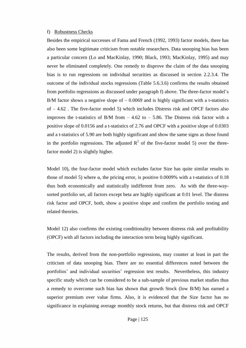
Page | 125
f) Robustness Checks
Besides the empirical successes of Fama and French (1992, 1993) factor models, there has
also been some legitimate criticism from notable researchers. Data snooping bias has been
a particular concern (Lo and MacKinlay, 1990; Black, 1993; MacKinlay, 1995) and may
never be eliminated completely. One remedy to disprove the claim of the data snooping
bias is to run regressions on individual securities as discussed in section 2.2.3.4. The
outcome of the individual stocks regressions (Table 5.6.3.6) confirms the results obtained
from portfolio regressions as discussed under paragraph f) above. The three-factor model’s
B/M factor shows a negative slope of – 0.0069 and is highly significant with a t-statistics
of – 4.62 . The five-factor model 5) which includes Distress risk and OPCF factors also
improves the t-statistics of B/M from – 4.62 to – 5.86. The Distress risk factor with a
positive slope of 0.0156 and a t-statistics of 2.76 and OPCF with a positive slope of 0.0303
and a t-statistics of 5.90 are both highly significant and show the same signs as those found
in the portfolio regressions. The adjusted R2 of the five-factor model 5) over the three-
factor model 2) is slightly higher.
Model 10), the four-factor model which excludes factor Size has quite similar results to
those of model 5) where α, the pricing error, is positive 0.0009% with a t-statistics of 0.18
thus both economically and statistically indifferent from zero. As with the three-way-
sorted portfolio set, all factors except beta are highly significant at 0.01 level. The distress
risk factor and OPCF, both, show a positive slope and confirm the portfolio testing and
related theories.
Model 12) also confirms the existing conditionality between distress risk and profitability
(OPCF) with all factors including the interaction term being highly significant.
The results, derived from the non-portfolio regressions, may counter at least in part the
criticism of data snooping bias. There are no essential differences noted between the
portfolios’ and individual securities’ regression test results. Nevertheless, this industry
specific study which can be considered to be a sub-sample of previous market studies thus
a remedy to overcome such bias has shown that growth Stock (low B/M) has earned a
superior premium over value firms. Also, it is evidenced that the Size factor has no
significance in explaining average monthly stock returns, but that distress risk and OPCF

Page | 126
factors when measured jointly are highly significant in doing so and that in a separate
setting both factors interact.
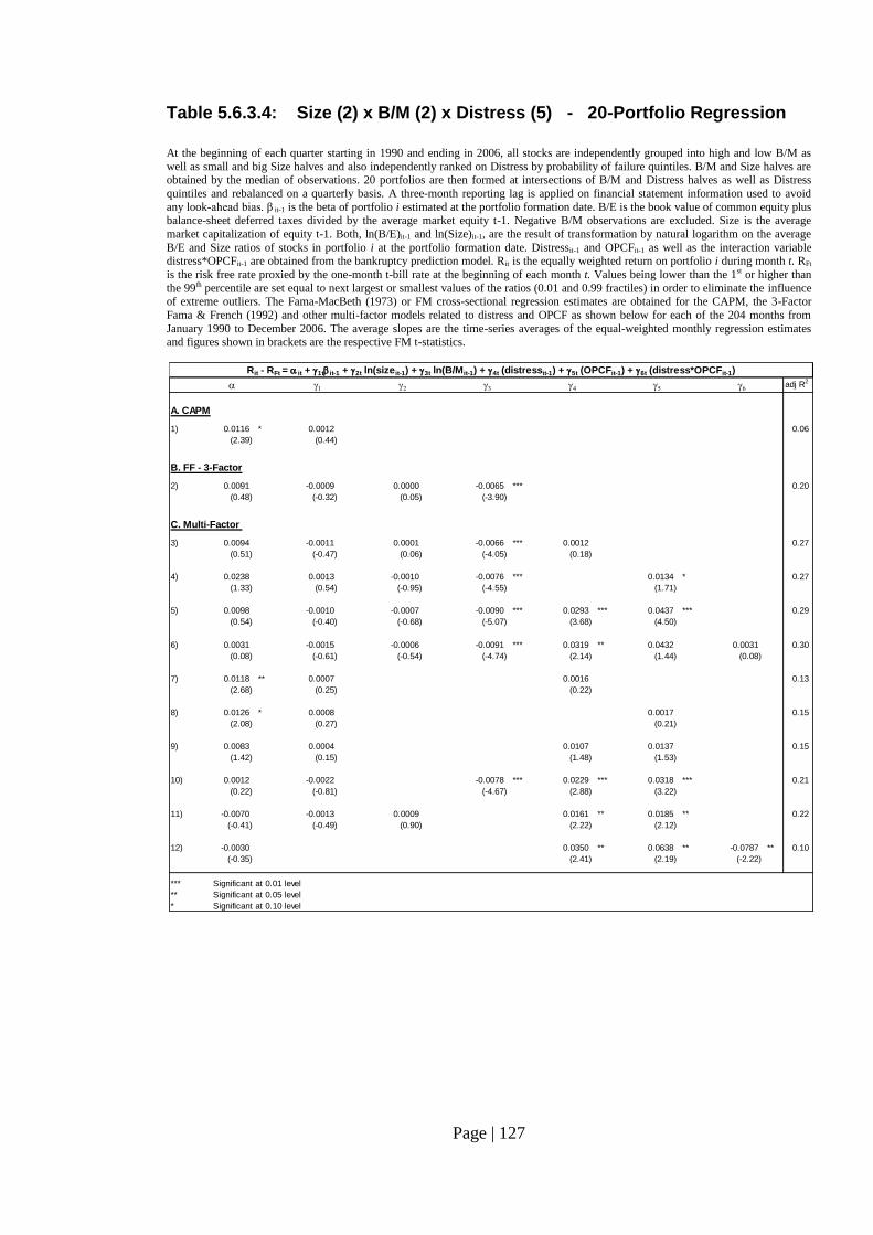
Page | 127
Table 5.6.3.4: Size (2) x B/M (2) x Distress (5) - 20-Portfolio Regression
At the beginning of each quarter starting in 1990 and ending in 2006, all stocks are independently grouped into high and low B/M as
well as small and big Size halves and also independently ranked on Distress by probability of failure quintiles. B/M and Size halves are obtained by the median of observations. 20 portfolios are then formed at intersections of B/M and Distress halves as well as Distress
quintiles and rebalanced on a quarterly basis. A three-month reporting lag is applied on financial statement information used to avoid
any look-ahead bias. β it-1 is the beta of portfolio i estimated at the portfolio formation date. B/E is the book value of common equity plus balance-sheet deferred taxes divided by the average market equity t-1. Negative B/M observations are excluded. Size is the average
market capitalization of equity t-1. Both, ln(B/E)it-1 and ln(Size)it-1, are the result of transformation by natural logarithm on the average
B/E and Size ratios of stocks in portfolio i at the portfolio formation date. Distressit-1 and OPCFit-1 as well as the interaction variable distress*OPCFit-1 are obtained from the bankruptcy prediction model. Rit is the equally weighted return on portfolio i during month t. RFt
is the risk free rate proxied by the one-month t-bill rate at the beginning of each month t. Values being lower than the 1st or higher than
the 99th percentile are set equal to next largest or smallest values of the ratios (0.01 and 0.99 fractiles) in order to eliminate the influence of extreme outliers. The Fama-MacBeth (1973) or FM cross-sectional regression estimates are obtained for the CAPM, the 3-Factor
Fama & French (1992) and other multi-factor models related to distress and OPCF as shown below for each of the 204 months from
January 1990 to December 2006. The average slopes are the time-series averages of the equal-weighted monthly regression estimates
and figures shown in brackets are the respective FM t-statistics.
1 2 3 4 5 6 adj R2
A. CAPM
1) 0.0116 * 0.0012 0.06
(2.39) (0.44)
B. FF - 3-Factor
2) 0.0091 -0.0009 0.0000 -0.0065 *** 0.20
(0.48) (-0.32) (0.05) (-3.90)
C. Multi-Factor
3) 0.0094 -0.0011 0.0001 -0.0066 *** 0.0012 0.27
(0.51) (-0.47) (0.06) (-4.05) (0.18)
4) 0.0238 0.0013 -0.0010 -0.0076 *** 0.0134 * 0.27
(1.33) (0.54) (-0.95) (-4.55) (1.71)
5) 0.0098 -0.0010 -0.0007 -0.0090 *** 0.0293 *** 0.0437 *** 0.29
(0.54) (-0.40) (-0.68) (-5.07) (3.68) (4.50)
6) 0.0031 -0.0015 -0.0006 -0.0091 *** 0.0319 ** 0.0432 0.0031 0.30
(0.08) (-0.61) (-0.54) (-4.74) (2.14) (1.44) (0.08)
7) 0.0118 ** 0.0007 0.0016 0.13
(2.68) (0.25) (0.22)
8) 0.0126 * 0.0008 0.0017 0.15
(2.08) (0.27) (0.21)
9) 0.0083 0.0004 0.0107 0.0137 0.15
(1.42) (0.15) (1.48) (1.53)
10) 0.0012 -0.0022 -0.0078 *** 0.0229 *** 0.0318 *** 0.21
(0.22) (-0.81) (-4.67) (2.88) (3.22)
11) -0.0070 -0.0013 0.0009 0.0161 ** 0.0185 ** 0.22
(-0.41) (-0.49) (0.90) (2.22) (2.12)
12) -0.0030 0.0350 ** 0.0638 ** -0.0787 ** 0.10
(-0.35) (2.41) (2.19) (-2.22)
*** Significant at 0.01 level
** Significant at 0.05 level
* Significant at 0.10 level
Rit - RFt = it + 1tit-1 + 2t ln(sizeit-1) + 3t ln(B/Mit-1) + 4t (distressit-1) + 5t (OPCFit-1) + 6t (distress*OPCFit-1)
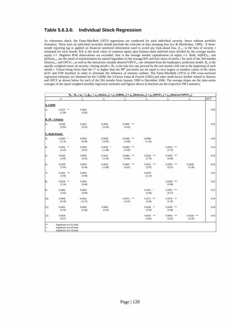
Page | 128
Table 5.6.3.6: Individual Stock Regression
As robustness check, the Fama-MacBeth (1973) regressions are conducted for each individual security, hence without portfolio
formation. These tests on individual securities should preclude the criticism of data snooping bias (Lo & MacKinlay, 1990). A three-month reporting lag is applied on financial statement information used to avoid any look-ahead bias. β it-1 is the beta of security i
estimated for each month. B/E is the book value of common equity plus balance-sheet deferred taxes divided by the average market
equity t-1. Negative B/M observations are excluded. Size is the average market capitalization of equity t-1. Both, ln(B/E)it-1 and ln(Size)it-1, are the result of transformation by natural logarithm on the average B/E and Size ratios of stocks i for each of the 204 months.
Distressit-1 and OPCFit-1 as well as the interaction variable distress*OPCFit-1 are obtained from the bankruptcy prediction model. Rit is the
equally weighted return on security i during month t. RFt is the risk free rate proxied by the one-month t-bill rate at the beginning of each month t. Values being lower than the 1st or higher than the 99th percentile are set equal to next largest or smallest values of the ratios
(0.01 and 0.99 fractiles) in order to eliminate the influence of extreme outliers. The Fama-MacBeth (1973) or FM cross-sectional
regression estimates are obtained for the CAPM, the 3-Factor Fama & French (1992) and other multi-factor models related to distress and OPCF as shown below for each of the 204 months from January 1990 to December 2006. The average slopes are the time-series
averages of the equal-weighted monthly regression estimates and figures shown in brackets are the respective FM t-statistics.
1 2 3 4 5 6 adj R2
A. CAPM
1) 0.0137 ** 0.0003 0.00
(2.39) (0.55)
B. FF - 3-Factor
2) 0.0165 0.0001 -0.0004 -0.0069 *** 0.02
(0.94) (0.15) (-0.45) (-4.62)
C. Multi-Factor
3) 0.0263 * 0.0002 -0.0008 -0.0066 *** -0.0086 0.03
(1.74) (0.49) (-0.92) (-4.80) (-1.41)
4) 0.0351 ** 0.0003 -0.0016 * -0.0082 *** 0.0231 *** 0.03
(2.25) (0.67) (-1.88) (-5.80) (4.75)
5) 0.0240 0.0002 -0.0013 -0.0083 *** 0.0156 *** 0.0303 *** 0.03
(1.59) (0.32) (-1.55) (-5.86) (2.76) (5.90)
6) 0.0239 0.0002 -0.0013 -0.0083 *** 0.0161 *** 0.0320 *** -0.0036 0.03
(1.54) (0.36) (-1.58) (-5.61) (2.67) (3.21) (-0.26)
7) 0.0161 *** 0.0003 -0.0078 0.01
(3.56) (0.69) (-1.13)
8) 0.0126 ** 0.0003 0.0168 *** 0.01
(2.14) (0.66) (3.08)
9) 0.0083 0.0003 0.0107 * 0.0222 *** 0.01
(1.62) (0.50) (1.83) (4.17)
10) 0.0009 -0.0001 -0.0071 *** 0.0171 *** 0.0279 *** 0.02
(0.18) (-0.12) (-5.02) (2.89) (5.10)
11) 0.0022 0.0002 0.0003 0.0128 ** 0.0229 *** 0.03
(0.15) (0.36) (0.42) (2.29) (4.49)
12) 0.0026 0.0224 *** 0.0453 *** -0.0318 *** 0.02
(0.47) (3.81) (4.51) (-2.55)
*** Significant at 0.01 level
** Significant at 0.05 level
* Significant at 0.10 level
Rit - RFt = it + 1tit-1 + 2t ln(sizeit-1) + 3t ln(B/Mit-1) + 4t (distressit-1) + 5t (OPCFit-1) + 6t (distress*OPCFit-1)
Page | 129
5.6.4 Asset Pricing Tests: Summary Result and Conclusion
The descriptive statistics (5.6.1), the correlation tests (5.6.2) and the Fama-MacBeth (1973)
cross-sectional regression tests (5.6.3) lead to the following results:
The descriptive statistics of table 5.6.1.1 show that on average, highly distressed stocks do
underperform non-distressed stocks. Distress deciles with probability of failure larger than
0.50 show a strong shortfall in mean excess returns when comparing to the group of non-
bankrupt firms at 8th
distress decile but also when benchmarking with the lowest distress
risk portfolios (Figure 5.6.1.1) This finding is consistent with Dichev (1998), Campbell,
Hilscher and Szilagyi (2008) as well as Agarwal and Taffler (2008). Given the descriptive
test results I conclude that hypothesis H2Aa) as shown in alternative form below cannot be
rejected.
H2Aa) Distressed stocks underperform on average non-distressed stocks.
The results (section 5.6.2) of the Pearson correlation tests performed on a portfolio by
portfolio as well as on an individual stock basis clearly indicate that bankruptcy risk is
independent from both the Size and B/M factors. Also, this study reveals that the B/M
factor follows an inverted u-shape along the distress risk deciles axis (section 5.6.1, figure
5.6.1.4) which means that highly distressed stocks are found in the low B/M quartile in
contrast to Fama and French’s (1992) distress factor proposition which would expect to
have high distressed stocks to be linked to high B/M values. This non-linear relationship
with the distress risk factor derived from a bankruptcy prediction model supports the
results of the Pearson correlation tests. The Fama-MacBeth (1973) cross-sectional
regressions show that a five-factor analysis consisting of Fama and French (1992) three-
factors plus Distress risk and profitability (OPCF) improve the B/M and Size factors’
significance level as reflected by related t-statistics. If B/M or Size were capturing the
distress factor, the inclusion of this study’s distress factor should have weakened either the
B/M and Size factors’ explanatory power or rejected the distress risk factor by its low t-
statistics. Furthermore, the addition of these two highly significant variables improved the
models’ overall explanatory power (higher adjusted R2). The intercepts of this excess
return model remained economically and statistically indifferent from zero. Assuming that
the bankruptcy prediction model’s probability of failure serves as a valid proxy for the
Page | 130
relative distress risk I can conclude that both Fama and French factors (1992) do not
capture bankruptcy risk. Given the descriptive (5.6.1, 5.6.2) and inferential statistics’ (5.6.3)
test results I conclude that hypothesis H2Ab) as shown in alternative form below cannot be
rejected.
H2Ab): The Fama-French (1992, 1993) distress factor hypothesis where both size
and B/M factors proxy distress risk does not hold.
The descriptive statistics (5.6.1) of Tables 5.6.1.1, 5.6.1.6 and in particular Figure 5.6.1.33
show that on average only highly distressed stock that is profitable may overperform non-
distressed stocks. Highly distressed but non-profitable portfolios as reflected by negative
OPCF earn on average lower stock returns.
The cross-sectional regressions as shown by Table 5.6.3.4 show that model 10) with proxy
factors for the risk based rational pricing proposition (distress factor) and the earnings
levels to returns proposition (OPCF) dominates the Fama-French (1992) three factor model
in describing excess returns as reflected by its slightly higher adjusted R2. The B/M factor
shows an improved t-statistics by the inclusion of the statistically significant distress risk
and profitability factors. Both, distress risk and profitability (OPCF) have positive slopes
and are in joint settings statistically significant as shown by Fama-MacBeth t-statistics,
hence confirming the two theoretical propositions of risk based rational pricing and the
positive relationship between earnings levels and stock returns as well as the result of
descriptive statistics. The separate testing of the interaction variable distress risk and
profitability confirms the conditional relationship between the two factors. Given the
descriptive (5.6.1) and inferential statistics’ (5.6.3) test results above and the non-rejection
of H2Aa), H2Ab) I conclude that hypothesis H2Ac) as shown in alternative form below
cannot be rejected.
H2Ac): The anomalous market underperformance of distressed stock can be
explained by a parallel analysis of risk based rational pricing and
profitability/earnings levels to returns propositions.
Overall, I conclude that an anomalous underperformance of distressed stocks can be
explained by the parallel application of risk based rational pricing and profitability levels
to return propositions .

Page | 131
On average, distressed stocks earn lower returns than non-distressed ones, a finding which
is consistent with Dichev (1998), Campbell, Hilscher, Szilagyi (2006) and Agarwal and
Taffler (2008). However, once the conditional relationship with profitability is taken into
account, the distress risk is rewarded by a continuous positive return hence priced
appropriately. Two-thirds of the highly distressed companies have low or negative excess
returns associated with negative profitability strength. The other third of distressed
companies is profitable and earn on average superior returns compared to a) their non-
distressed counterparts and b) distressed but non-profitable companies. Profitability (OPCF)
is also found to be positively associated with stock returns hence in line with the earnings
levels to returns relationship proposition.
Besides the joint pricing of relative distress risk and profitability levels (OPCF), the study
makes clear that the distress factor hypothesis as proposed by Fama and French (1992)
does not hold. Highly distressed companies have a similar low B/M profile as low distress
firms do hence it cannot support a linear relationship to relative distress risk derived from a
bankruptcy prediction model. However, the B/M factor’s inverted u-shape actually mirrors
the excess stock returns along the distress deciles quite well. That is why it is technically
speaking highly significant in explaining stock returns.
Page | 132
CHAPTER 6: CONCLUSION
6.1 Conclusion
The main purpose of this study is to find out if the anomalous market underperformance of
distressed stock can be explained by a parallel analysis of risk based pricing and
profitability/(earnings) levels to returns relationship propositions. When the conditional
relationship with profitability is taken into account, the distress risk is rewarded by a
continuous positive return hence priced appropriately. In addition, the distress risk factor
is derived from a cash flow based bankruptcy prediction model. In this study I aim to show
that a cash flow based hazard model predicts bankruptcies at higher accuracy rates than its
benchmark, the Altman’s Z-score model.
6.1.1 Contribution to Knowledge
Two main contributions are made to the literature of prediction and pricing of relative
distress risk.
First, for the pricing of the distress risk and profitability factors various portfolios have
been formed and factors calculated on an equal-weighted basis. The portfolios are
rebalanced on a quarterly basis using only publicly available data at the formation date
assuming a three-month reporting lag. The descriptive statistics emerged from the portfolio
formation and factor calculations based on time-series averages over 204 months (1990 –
2006) have been provided on a portfolio by portfolio basis. In addition, Pearson
correlation tests have been conducted to check for multicollinearity and to obtain results in
connection with the distress factor hypothesis. Last but not least, Fama-MacBeth (1973)
cross-sectional regressions have been run on various sets of portfolios to obtain t-statistics
and adj. R2 for different types of models such as CAPM, Fama-French (1992) three-factor
model and augmentations. This also included the four-factor model with beta, B/M, the
relative distress risk and profitability strength (OPCF) factors to perform the parallel
analysis of the two propositions as mentioned above. In addition, I have also tested for a
potential conditionality between the two factors.
Page | 133
First, I can show that the anomalous underperformance of distressed stocks in the US
computer and electronics industry can be explained by the parallel analysis of the risk
based rational pricing and the profitability levels to returns relationship propositions.
There is evidence that distressed stocks earn a positive continuous distress risk premium
and that they are appropriately priced once the conditionality with profitability is taken into
account.
Second, a cash flow based hazard model which predicts bankruptcies at higher accuracy
rates than Altman’s (1968) Z-score, as evidenced by a ROC benchmark model, has been
developed. This industry specific model uses in contrast to many other studies non-
arbitrarily selected cash flow variables derived from Lawson’ cash flow identity (1971).
This econometric model is constructed on the grounds of one of the more recent
developments in this field by employing a hazard model (Shumway, 2001; Beaver,
McNichols and Rhie, 2004; Campbell, Hilscher and Szilagyi, 2008). The model’s
prediction outcomes are validated by confirmative out-of-sample and favourable
benchmark test results and can be considered to be robust. This model, a Cox proportional
hazard model, not only predicts corporate failure, but also produces the probabilities of
failure for each firm on quarterly basis which serve as a proxy for the continuous relative
distress risk factor to be included in asset pricing tests as mentioned before.
Besides the joint pricing of relative distress risk and current profitability levels the study
shows that the distress factor hypothesis as proposed by Fama and French (1992) does not
hold. Highly distressed companies have a similarly low B/M profile as low distress firms.
The inverted u-shape of B/M values along the distress risk deciles axis is in line with
Dichev’s (1998) finding. As result, it cannot support a linear relationship to the relative
distress risk derived from a bankruptcy prediction model. The B/M and/or Size factors may
capture something else with or without an involvement of relative distress risk.
Page | 134
6.1.2 Limitations
Bankruptcy prediction models are widely used in practice and in the literature but they lack
a coherent theoretical basis. Jones (1987) argues that the prediction of firms’ bankruptcies
in temporal and economic settings different from then when the models are developed
makes it rather difficult to ascertain whether such procedure is appropriate. Like other
models, the one in this study measures bankruptcy risks with errors.
Although, there is a lack of bankruptcy theory, these empirical findings may contribute to
the knowledge of better understanding the phenomenon of bankruptcy by providing
economic interpretations.
There are also limitations given from a time and industry perspective. The data used for
the asset pricing tests cover the period from 1990 to 2006. The financial data to be used for
the calculation of the probabilities of failure is drawn from a statement of cash flows as
required by Statement of Financial Accounting Standards (SFAS) No. 95. This Statement
has been effective for firms reporting annual financial statements for fiscal years ending
after July 15, 1988. The bankruptcy prediction model requires four quarters’ rolling cash
flow data so that the first probability of failure is obtained for the second quarter in 1989.
In order to avoid a look-ahead bias in asset pricing tests a three-month lag between quarter
or year end and reporting of financial statements is assumed. The earliest availability of
historical data would have been at beginning of the 4th
quarter in 1989. For simplicity and
completeness reasons the first month used for asset pricing tests in this study is January
1990. An expansion of prior periods would require a different approach in calculating the
needed cash flow variables. The bankruptcy prediction model as well as the asset pricing
models’ test results are limited to the computer and electronics industry (NAICS code 334).
Therefore, drawing statistical inferences from these models outside this specific industry is
rather prohibitive but it could be an area for future research.
The cross-sectional regression results of the asset pricing tests are subject to several known
limitations. First, the market return used for the calculation of market beta is the S&P 500
Page | 135
index which itself cannot be considered to be the entire “true” market portfolio. Therefore,
CAPM’s inability to describe returns in this study cannot automatically lead to a rejection
of the model (Roll, 1977). Kothari, Shanken and Sloan (1995) argue that annual betas are
more appropriate than monthly ones since the investment horizon for a typical investor is
probably closer to a year. The beta could be estimated using a different convention than
applied in this study and consequently could have produced higher significance in
explaining stock returns. Multi-factor models such as Fama and French (1992, 1993) which
are able to describe monthly stock returns successfully may be the result of data snooping
(Black, 1993; MacKinlay, 1995). The study has been designed to counter this accusation.
The asset pricing models are tested for an association measurement between financial
statements’ derived factors and stock returns. Investors have access to many more
information sources about a company’s distress risk and cash flow generating ability. The
Statement of Financial Accounting Standards (SFAS) No. 95 has been used to calculate
distress risk and operating cash flow strengths for companies in the US computer and
electronics industry and can be considered to be a proxy or substitute for investors’
available information at hand when making their investment decisions. Nevertheless, as
Kothari (2001) points out, there is no causal connection between such accounting
information and stock prices and their movements to be inferred.
Haugen and Baker (1996) see two different groups of explaining differentials in stock
returns. The first one supports a risk based rational pricing hypothesis (Fama and French,
1992, 1993, 1996; Ball, Kothari and Shanken, 1995) and the second group view these
differentials in predicted returns as surprise to investors as result of market over- and
underreactions related factors (Chopra, Lakonishok and Ritter, 1992; Lakonishok, Shleifer,
Vishny, 1994; Haugen, 1995; and others). They find it rather difficult to link an
underperformance of distressed stock to a rational asset pricing explanation as in their
studies distressed stocks showing conflicting but expected characteristics of higher beta,
higher B/M and smaller size. So, this group rather believes in a pricing bias hypothesis.
I provide a parallel analysis of two propositions, the risk based rational pricing and the
positive relationship between profitability/earnings levels and returns, which can explain
the underperformance of highly distressed stocks once the conditional relationship with

Page | 136
profitability levels is taken into account. The study shows that distressed stocks are
appropriately priced. However, the question remains why and under what rational or
irrational assumptions investors would get involved in highly distressed and loss making
investments. This is a topic for further research.
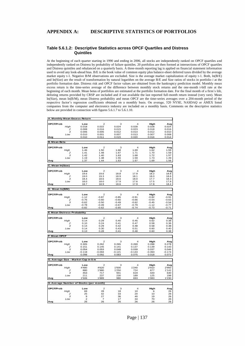
Page | 137
APPENDIX A: DESCRIPTIVE STATISTICS OF PORTFOLIOS
Table 5.6.1.2: Descriptive Statistics across OPCF Quartiles and Distress Quintiles At the beginning of each quarter starting in 1990 and ending in 2006, all stocks are independently ranked on OPCF quartiles and
independently ranked on Distress by probability of failure quintiles. 20 portfolios are then formed at intersections of OPCF quartiles and Distress quintiles and rebalanced on a quarterly basis. A three-month reporting lag is applied on financial statement information
used to avoid any look-ahead bias. B/E is the book value of common equity plus balance-sheet deferred taxes divided by the average
market equity t-1. Negative B/M observations are excluded. Size is the average market capitalization of equity t-1. Both, ln(B/E) and ln(Size) are the result of transformation by natural logarithm on the average B/E and Size ratios of stocks in portfolio i at the
portfolio formation date. Distress risk and OPCF factor values are obtained from the bankruptcy prediction model. Monthly mean
excess return is the time-series average of the difference between monthly stock returns and the one-month t-bill rate at the beginning of each month. Mean betas of portfolios are estimated at the portfolio formation date. For the final month of a firm’s life,
delisting returns provided by CRSP are included and if not available the last reported full-month return instead (very rare). Mean
ln(Size), mean ln(B/M), mean Distress probability and mean OPCF are the time-series averages over a 204-month period of the respective factor’s regression coefficients obtained on a monthly basis. On average, 520 NYSE, NASDAQ or AMEX listed
companies from the computer and electronics industry are included on a monthly basis. Comments on the descriptive statistics
below are provided in connection with figures 5.6.1.7 to 5.6.1.10.
A. Monthly Mean Excess Return
OPCF/Prob Low 2 3 4 High Avg
High 0.018 0.022 0.024 0.028 0.028 0.024
2 0.008 0.016 0.015 0.023 0.018 0.016
3 0.006 0.005 0.012 0.014 0.012 0.010
Low 0.010 0.001 0.007 0.013 0.007 0.008
Avg 0.010 0.011 0.015 0.020 0.016 0.014
B. Mean Beta
OPCF/Prob Low 2 3 4 High Avg
High 1.46 1.50 1.68 1.69 1.62 1.59
2 1.41 1.48 1.67 1.71 1.70 1.59
3 1.42 1.40 1.63 1.68 1.72 1.57
Low 1.19 1.38 1.55 1.59 1.73 1.49
Avg 1.37 1.44 1.63 1.67 1.69 1.56
C. Mean ln(Size)
OPCF/Prob Low 2 3 4 High Avg
High 19.6 19.6 18.8 17.9 18.2 18.8
2 19.0 19.3 18.9 18.1 18.0 18.6
3 18.4 18.6 18.6 18.0 17.7 18.3
Low 18.0 18.0 17.9 17.6 17.5 17.8
Avg 18.7 18.9 18.6 17.9 17.8 18.4
D. Mean ln(B/M)
OPCF/Prob Low 2 3 4 High Avg
High -1.12 -0.87 -0.85 -0.91 -0.82 -0.91
2 -0.76 -0.60 -0.60 -0.66 -0.54 -0.63
3 -0.62 -0.50 -0.49 -0.62 -0.45 -0.54
Low -0.78 -0.49 -0.67 -0.79 -1.12 -0.77
Avg -0.82 -0.62 -0.65 -0.74 -0.73 -0.71
E. Mean Distress Probability
OPCF/Prob Low 2 3 4 High Avg
High 0.14 0.29 0.40 0.45 0.62 0.38
2 0.10 0.24 0.41 0.47 0.58 0.36
3 0.14 0.29 0.42 0.48 0.58 0.38
Low 0.14 0.30 0.43 0.51 0.60 0.40
Avg 0.13 0.28 0.41 0.48 0.60 0.38
F. Mean OPCF
OPCF/Prob Low 2 3 4 High Avg
High 0.305 0.262 0.265 0.269 0.288 0.278
2 0.151 0.145 0.141 0.137 0.139 0.143
3 0.054 0.053 0.048 0.039 0.037 0.046
Low -0.118 -0.094 -0.121 -0.143 -0.393 -0.174
Avg 0.098 0.092 0.083 0.075 0.018 0.073
G. Average Size - Market Cap in $ m
OPCF/Prob Low 2 3 4 High Avg
High 4'480 4'620 1'500 1'240 2'910 2'950
2 880 1'980 1'250 724 877 1'142
3 453 717 941 619 420 630
Low 211 237 230 189 125 198
Avg 1'506 1'889 980 693 1'083 1'230
H. Average Number of Stocks (per month)
OPCF/Prob Low 2 3 4 High Avg
High 69 28 18 10 6 26
2 25 42 33 20 10 26
3 9 27 36 40 19 26
Low 2 7 17 34 70 26
Avg 26 26 26 26 26 26
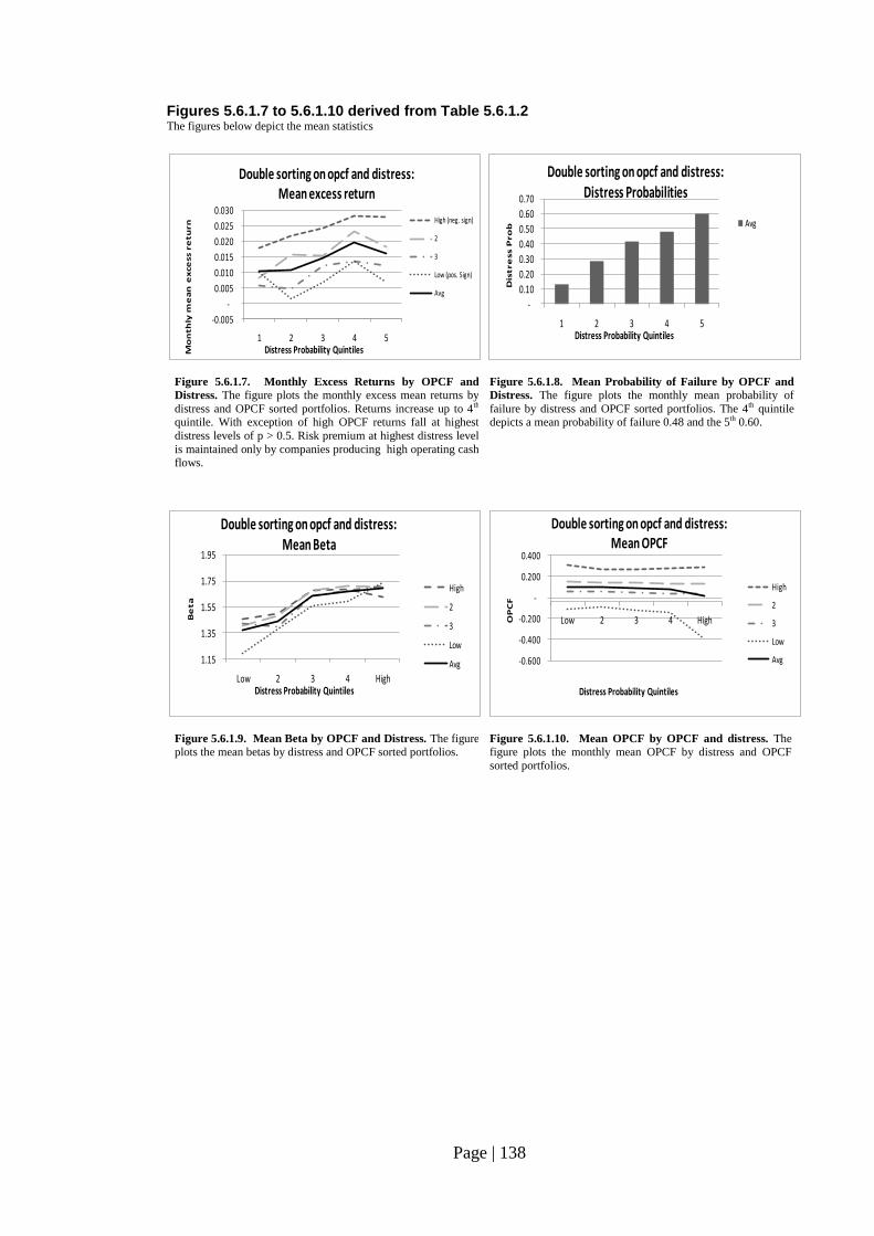
Page | 138
Figures 5.6.1.7 to 5.6.1.10 derived from Table 5.6.1.2 The figures below depict the mean statistics
Figure 5.6.1.7. Monthly Excess Returns by OPCF and
Distress. The figure plots the monthly excess mean returns by
distress and OPCF sorted portfolios. Returns increase up to 4th quintile. With exception of high OPCF returns fall at highest
distress levels of p > 0.5. Risk premium at highest distress level
is maintained only by companies producing high operating cash flows.
Figure 5.6.1.8. Mean Probability of Failure by OPCF and
Distress. The figure plots the monthly mean probability of
failure by distress and OPCF sorted portfolios. The 4th quintile depicts a mean probability of failure 0.48 and the 5th 0.60.
Figure 5.6.1.9. Mean Beta by OPCF and Distress. The figure plots the mean betas by distress and OPCF sorted portfolios.
Figure 5.6.1.10. Mean OPCF by OPCF and distress. The figure plots the monthly mean OPCF by distress and OPCF
sorted portfolios.
-0.005
-
0.005
0.010
0.015
0.020
0.025
0.030
1 2 3 4 5
Mo
nth
ly m
ea
n e
xce
ss r
etu
rn
Distress Probability Quintiles
Double sorting on opcf and distress: Mean excess return
High (neg. sign)
2
3
Low (pos. Sign)
Avg
-
0.10
0.20
0.30
0.40
0.50
0.60
0.70
1 2 3 4 5
Dis
tre
ss P
ro
b
Distress Probability Quintiles
Double sorting on opcf and distress: Distress Probabilities
Avg
1.15
1.35
1.55
1.75
1.95
Low 2 3 4 High
Be
ta
Distress Probability Quintiles
Double sorting on opcf and distress: Mean Beta
High
2
3
Low
Avg -0.600
-0.400
-0.200
-
0.200
0.400
Low 2 3 4 HighOP
CF
Distress Probability Quintiles
Double sorting on opcf and distress: Mean OPCF
High
2
3
Low
Avg
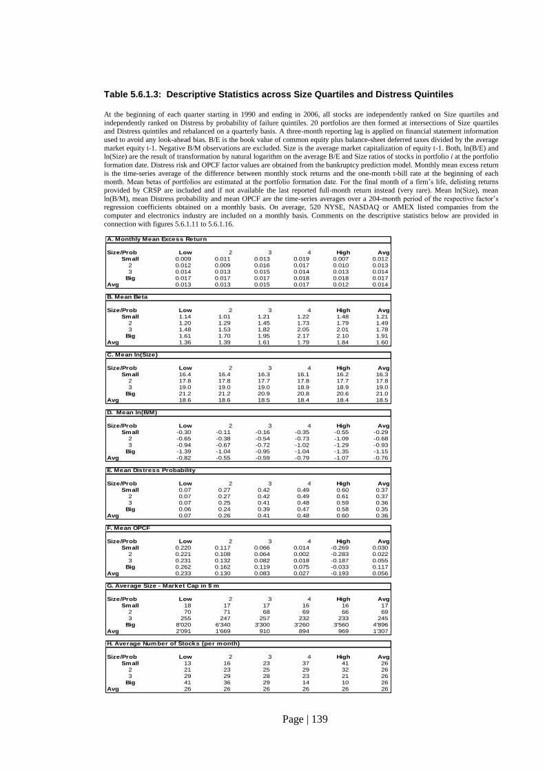
Page | 139
Table 5.6.1.3: Descriptive Statistics across Size Quartiles and Distress Quintiles At the beginning of each quarter starting in 1990 and ending in 2006, all stocks are independently ranked on Size quartiles and
independently ranked on Distress by probability of failure quintiles. 20 portfolios are then formed at intersections of Size quartiles and Distress quintiles and rebalanced on a quarterly basis. A three-month reporting lag is applied on financial statement information
used to avoid any look-ahead bias. B/E is the book value of common equity plus balance-sheet deferred taxes divided by the average
market equity t-1. Negative B/M observations are excluded. Size is the average market capitalization of equity t-1. Both, ln(B/E) and ln(Size) are the result of transformation by natural logarithm on the average B/E and Size ratios of stocks in portfolio i at the portfolio
formation date. Distress risk and OPCF factor values are obtained from the bankruptcy prediction model. Monthly mean excess return
is the time-series average of the difference between monthly stock returns and the one-month t-bill rate at the beginning of each month. Mean betas of portfolios are estimated at the portfolio formation date. For the final month of a firm’s life, delisting returns
provided by CRSP are included and if not available the last reported full-month return instead (very rare). Mean ln(Size), mean
ln(B/M), mean Distress probability and mean OPCF are the time-series averages over a 204-month period of the respective factor’s regression coefficients obtained on a monthly basis. On average, 520 NYSE, NASDAQ or AMEX listed companies from the
computer and electronics industry are included on a monthly basis. Comments on the descriptive statistics below are provided in
connection with figures 5.6.1.11 to 5.6.1.16.
A. Monthly Mean Excess Return
Size/Prob Low 2 3 4 High Avg
Small 0.009 0.011 0.013 0.019 0.007 0.012
2 0.012 0.009 0.016 0.017 0.010 0.013
3 0.014 0.013 0.015 0.014 0.013 0.014
Big 0.017 0.017 0.017 0.018 0.018 0.017
Avg 0.013 0.013 0.015 0.017 0.012 0.014
B. Mean Beta
Size/Prob Low 2 3 4 High Avg
Small 1.14 1.01 1.21 1.22 1.48 1.21
2 1.20 1.29 1.45 1.73 1.79 1.49
3 1.48 1.53 1.82 2.05 2.01 1.78
Big 1.61 1.70 1.95 2.17 2.10 1.91
Avg 1.36 1.39 1.61 1.79 1.84 1.60
C. Mean ln(Size)
Size/Prob Low 2 3 4 High Avg
Small 16.4 16.4 16.3 16.1 16.2 16.3
2 17.8 17.8 17.7 17.8 17.7 17.8
3 19.0 19.0 19.0 18.9 18.9 19.0
Big 21.2 21.2 20.9 20.8 20.6 21.0
Avg 18.6 18.6 18.5 18.4 18.4 18.5
D. Mean ln(B/M)
Size/Prob Low 2 3 4 High Avg
Small -0.30 -0.11 -0.16 -0.35 -0.55 -0.29
2 -0.65 -0.38 -0.54 -0.73 -1.09 -0.68
3 -0.94 -0.67 -0.72 -1.02 -1.29 -0.93
Big -1.39 -1.04 -0.95 -1.04 -1.35 -1.15
Avg -0.82 -0.55 -0.59 -0.79 -1.07 -0.76
E. Mean Distress Probability
Size/Prob Low 2 3 4 High Avg
Small 0.07 0.27 0.42 0.49 0.60 0.37
2 0.07 0.27 0.42 0.49 0.61 0.37
3 0.07 0.25 0.41 0.48 0.59 0.36
Big 0.06 0.24 0.39 0.47 0.58 0.35
Avg 0.07 0.26 0.41 0.48 0.60 0.36
F. Mean OPCF
Size/Prob Low 2 3 4 High Avg
Small 0.220 0.117 0.066 0.014 -0.269 0.030
2 0.221 0.108 0.064 0.002 -0.283 0.022
3 0.231 0.132 0.082 0.018 -0.187 0.055
Big 0.262 0.162 0.119 0.075 -0.033 0.117
Avg 0.233 0.130 0.083 0.027 -0.193 0.056
G. Average Size - Market Cap in $ m
Size/Prob Low 2 3 4 High Avg
Small 18 17 17 16 16 17
2 70 71 68 69 66 69
3 255 247 257 232 233 245
Big 8'020 6'340 3'300 3'260 3'560 4'896
Avg 2'091 1'669 910 894 969 1'307
H. Average Number of Stocks (per month)
Size/Prob Low 2 3 4 High Avg
Small 13 16 23 37 41 26
2 21 23 25 29 32 26
3 29 29 28 23 21 26
Big 41 36 29 14 10 26
Avg 26 26 26 26 26 26
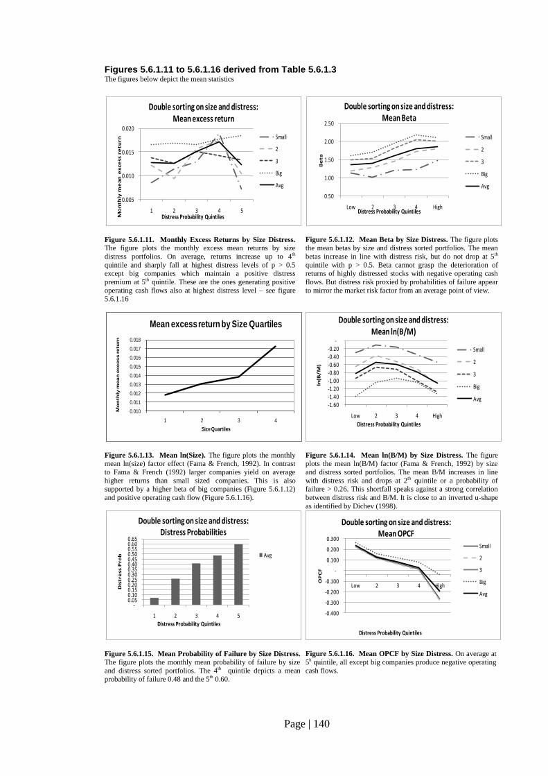
Page | 140
Figures 5.6.1.11 to 5.6.1.16 derived from Table 5.6.1.3 The figures below depict the mean statistics
Figure 5.6.1.11. Monthly Excess Returns by Size Distress.
The figure plots the monthly excess mean returns by size
distress portfolios. On average, returns increase up to 4th
quintile and sharply fall at highest distress levels of p > 0.5 except big companies which maintain a positive distress
premium at 5th quintile. These are the ones generating positive
operating cash flows also at highest distress level – see figure 5.6.1.16
Figure 5.6.1.12. Mean Beta by Size Distress. The figure plots the mean betas by size and distress sorted portfolios. The mean
betas increase in line with distress risk, but do not drop at 5th
quintile with p > 0.5. Beta cannot grasp the deterioration of returns of highly distressed stocks with negative operating cash
flows. But distress risk proxied by probabilities of failure appear
to mirror the market risk factor from an average point of view.
Figure 5.6.1.13. Mean ln(Size). The figure plots the monthly mean ln(size) factor effect (Fama & French, 1992). In contrast
to Fama & French (1992) larger companies yield on average
higher returns than small sized companies. This is also supported by a higher beta of big companies (Figure 5.6.1.12)
and positive operating cash flow (Figure 5.6.1.16).
Figure 5.6.1.14. Mean ln(B/M) by Size Distress. The figure plots the mean ln(B/M) factor (Fama & French, 1992) by size
and distress sorted portfolios. The mean B/M increases in line
with distress risk and drops at 2th quintile or a probability of failure > 0.26. This shortfall speaks against a strong correlation
between distress risk and B/M. It is close to an inverted u-shape
as identified by Dichev (1998).
Figure 5.6.1.15. Mean Probability of Failure by Size Distress.
The figure plots the monthly mean probability of failure by size
and distress sorted portfolios. The 4th quintile depicts a mean probability of failure 0.48 and the 5th 0.60.
Figure 5.6.1.16. Mean OPCF by Size Distress. On average at
5h quintile, all except big companies produce negative operating
cash flows.
0.005
0.010
0.015
0.020
1 2 3 4 5
Mo
nth
ly m
ea
n e
xce
ss r
etu
rn
Distress Probability Quintiles
Double sorting on size and distress: Mean excess return
Small
2
3
Big
Avg
0.50
1.00
1.50
2.00
2.50
Low 2 3 4 High
Be
ta
Distress Probability Quintiles
Double sorting on size and distress: Mean Beta
Small
2
3
Big
Avg
0.010
0.011
0.012
0.013
0.014
0.015
0.016
0.017
0.018
1 2 3 4
Mo
nth
ly m
ean
excess retu
rn
Size Quartiles
Mean excess return by Size Quartiles
-1.60 -1.40 -1.20 -1.00 -0.80 -0.60 -0.40 -0.20
-
Low 2 3 4 High
ln(B
/M
)
Distress Probability Quintiles
Double sorting on size and distress: Mean ln(B/M)
Small
2
3
Big
Avg
-0.05 0.10 0.15 0.20 0.25 0.30 0.35 0.40 0.45 0.50 0.55 0.60 0.65
1 2 3 4 5
Dis
tre
ss P
rob
Distress Probability Quintiles
Double sorting on size and distress: Distress Probabilities
Avg
-0.400
-0.300
-0.200
-0.100
-
0.100
0.200
0.300
Low 2 3 4 High
OP
CF
Distress Probability Quintiles
Double sorting on size and distress: Mean OPCF
Small
2
3
Big
Avg
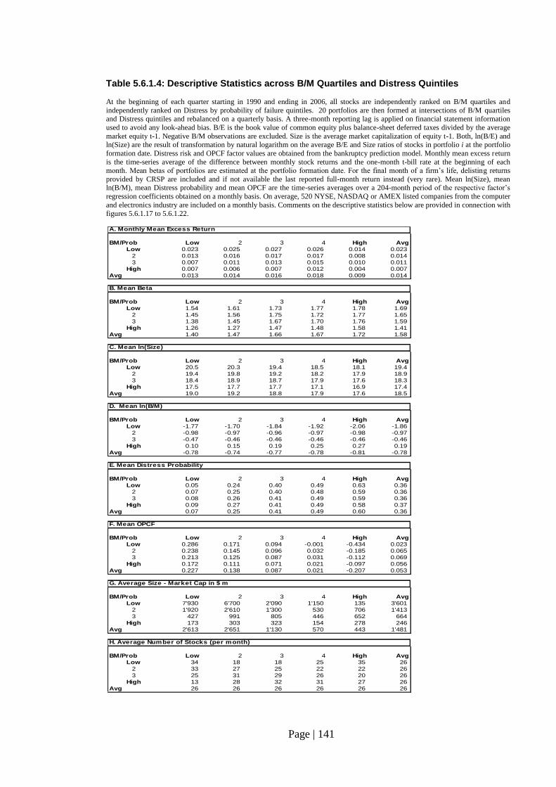
Page | 141
Table 5.6.1.4: Descriptive Statistics across B/M Quartiles and Distress Quintiles At the beginning of each quarter starting in 1990 and ending in 2006, all stocks are independently ranked on B/M quartiles and
independently ranked on Distress by probability of failure quintiles. 20 portfolios are then formed at intersections of B/M quartiles and Distress quintiles and rebalanced on a quarterly basis. A three-month reporting lag is applied on financial statement information
used to avoid any look-ahead bias. B/E is the book value of common equity plus balance-sheet deferred taxes divided by the average
market equity t-1. Negative B/M observations are excluded. Size is the average market capitalization of equity t-1. Both, ln(B/E) and ln(Size) are the result of transformation by natural logarithm on the average B/E and Size ratios of stocks in portfolio i at the portfolio
formation date. Distress risk and OPCF factor values are obtained from the bankruptcy prediction model. Monthly mean excess return
is the time-series average of the difference between monthly stock returns and the one-month t-bill rate at the beginning of each month. Mean betas of portfolios are estimated at the portfolio formation date. For the final month of a firm’s life, delisting returns
provided by CRSP are included and if not available the last reported full-month return instead (very rare). Mean ln(Size), mean ln(B/M), mean Distress probability and mean OPCF are the time-series averages over a 204-month period of the respective factor’s
regression coefficients obtained on a monthly basis. On average, 520 NYSE, NASDAQ or AMEX listed companies from the computer
and electronics industry are included on a monthly basis. Comments on the descriptive statistics below are provided in connection with
figures 5.6.1.17 to 5.6.1.22.
A. Monthly Mean Excess Return
BM/Prob Low 2 3 4 High Avg
Low 0.023 0.025 0.027 0.026 0.014 0.023
2 0.013 0.016 0.017 0.017 0.008 0.014
3 0.007 0.011 0.013 0.015 0.010 0.011
High 0.007 0.006 0.007 0.012 0.004 0.007
Avg 0.013 0.014 0.016 0.018 0.009 0.014
B. Mean Beta
BM/Prob Low 2 3 4 High Avg
Low 1.54 1.61 1.73 1.77 1.78 1.69
2 1.45 1.56 1.75 1.72 1.77 1.65
3 1.38 1.45 1.67 1.70 1.76 1.59
High 1.26 1.27 1.47 1.48 1.58 1.41
Avg 1.40 1.47 1.66 1.67 1.72 1.58
C. Mean ln(Size)
BM/Prob Low 2 3 4 High Avg
Low 20.5 20.3 19.4 18.5 18.1 19.4
2 19.4 19.8 19.2 18.2 17.9 18.9
3 18.4 18.9 18.7 17.9 17.6 18.3
High 17.5 17.7 17.7 17.1 16.9 17.4
Avg 19.0 19.2 18.8 17.9 17.6 18.5
D. Mean ln(B/M)
BM/Prob Low 2 3 4 High Avg
Low -1.77 -1.70 -1.84 -1.92 -2.06 -1.86
2 -0.98 -0.97 -0.96 -0.97 -0.98 -0.97
3 -0.47 -0.46 -0.46 -0.46 -0.46 -0.46
High 0.10 0.15 0.19 0.25 0.27 0.19
Avg -0.78 -0.74 -0.77 -0.78 -0.81 -0.78
E. Mean Distress Probability
BM/Prob Low 2 3 4 High Avg
Low 0.05 0.24 0.40 0.49 0.63 0.36
2 0.07 0.25 0.40 0.48 0.59 0.36
3 0.08 0.26 0.41 0.49 0.59 0.36
High 0.09 0.27 0.41 0.49 0.58 0.37
Avg 0.07 0.25 0.41 0.49 0.60 0.36
F. Mean OPCF
BM/Prob Low 2 3 4 High Avg
Low 0.286 0.171 0.094 -0.001 -0.434 0.023
2 0.238 0.145 0.096 0.032 -0.185 0.065
3 0.213 0.125 0.087 0.031 -0.112 0.069
High 0.172 0.111 0.071 0.021 -0.097 0.056
Avg 0.227 0.138 0.087 0.021 -0.207 0.053
G. Average Size - Market Cap in $ m
BM/Prob Low 2 3 4 High Avg
Low 7'930 6'700 2'090 1'150 135 3'601
2 1'920 2'610 1'300 530 706 1'413
3 427 991 805 446 652 664
High 173 303 323 154 278 246
Avg 2'613 2'651 1'130 570 443 1'481
H. Average Number of Stocks (per month)
BM/Prob Low 2 3 4 High Avg
Low 34 18 18 25 35 26
2 33 27 25 22 22 26
3 25 31 29 26 20 26
High 13 28 32 31 27 26
Avg 26 26 26 26 26 26
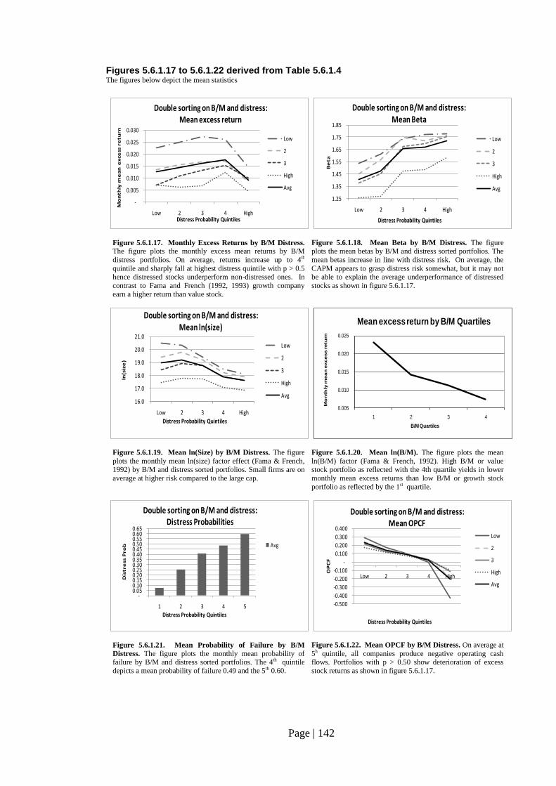
Page | 142
Figures 5.6.1.17 to 5.6.1.22 derived from Table 5.6.1.4 The figures below depict the mean statistics
Figure 5.6.1.17. Monthly Excess Returns by B/M Distress.
The figure plots the monthly excess mean returns by B/M
distress portfolios. On average, returns increase up to 4th
quintile and sharply fall at highest distress quintile with p > 0.5 hence distressed stocks underperform non-distressed ones. In
contrast to Fama and French (1992, 1993) growth company
earn a higher return than value stock.
Figure 5.6.1.18. Mean Beta by B/M Distress. The figure plots the mean betas by B/M and distress sorted portfolios. The
mean betas increase in line with distress risk. On average, the
CAPM appears to grasp distress risk somewhat, but it may not be able to explain the average underperformance of distressed
stocks as shown in figure 5.6.1.17.
Figure 5.6.1.19. Mean ln(Size) by B/M Distress. The figure
plots the monthly mean ln(size) factor effect (Fama & French, 1992) by B/M and distress sorted portfolios. Small firms are on
average at higher risk compared to the large cap.
Figure 5.6.1.20. Mean ln(B/M). The figure plots the mean
ln(B/M) factor (Fama & French, 1992). High B/M or value stock portfolio as reflected with the 4th quartile yields in lower
monthly mean excess returns than low B/M or growth stock
portfolio as reflected by the 1st quartile.
Figure 5.6.1.21. Mean Probability of Failure by B/M
Distress. The figure plots the monthly mean probability of failure by B/M and distress sorted portfolios. The 4th quintile
depicts a mean probability of failure 0.49 and the 5th 0.60.
Figure 5.6.1.22. Mean OPCF by B/M Distress. On average at
5h quintile, all companies produce negative operating cash flows. Portfolios with p > 0.50 show deterioration of excess
stock returns as shown in figure 5.6.1.17.
-
0.005
0.010
0.015
0.020
0.025
0.030
Low 2 3 4 High
Mo
nth
ly m
ea
n e
xce
ss r
etu
rn
Distress Probability Quintiles
Double sorting on B/M and distress: Mean excess return
Low
2
3
High
Avg
1.25
1.35
1.45
1.55
1.65
1.75
1.85
Low 2 3 4 High
Be
ta
Distress Probability Quintiles
Double sorting on B/M and distress: Mean Beta
Low
2
3
High
Avg
16.0
17.0
18.0
19.0
20.0
21.0
Low 2 3 4 High
ln(s
ize
)
Distress Probability Quintiles
Double sorting on B/M and distress: Mean ln(size)
Low
2
3
High
Avg
0.005
0.010
0.015
0.020
0.025
1 2 3 4
Mo
nth
ly m
ean
excess retu
rn
B/M Quartiles
Mean excess return by B/M Quartiles
-0.05 0.10 0.15 0.20 0.25 0.30 0.35 0.40 0.45 0.50 0.55 0.60 0.65
1 2 3 4 5
Dis
tre
ss P
rob
Distress Probability Quintiles
Double sorting on B/M and distress: Distress Probabilities
Avg
-0.500
-0.400
-0.300
-0.200
-0.100
-
0.100
0.200
0.300
0.400
Low 2 3 4 High
OP
CF
Distress Probability Quintiles
Double sorting on B/M and distress: Mean OPCF
Low
2
3
High
Avg
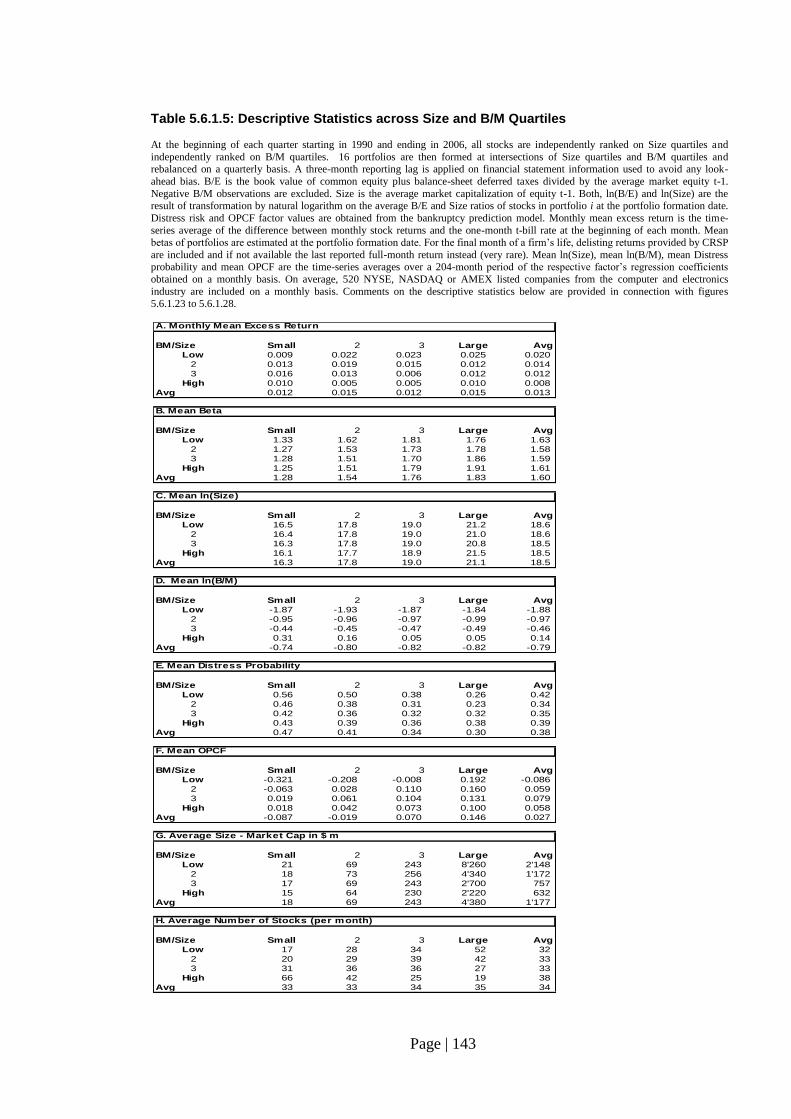
Page | 143
Table 5.6.1.5: Descriptive Statistics across Size and B/M Quartiles At the beginning of each quarter starting in 1990 and ending in 2006, all stocks are independently ranked on Size quartiles and
independently ranked on B/M quartiles. 16 portfolios are then formed at intersections of Size quartiles and B/M quartiles and rebalanced on a quarterly basis. A three-month reporting lag is applied on financial statement information used to avoid any look-
ahead bias. B/E is the book value of common equity plus balance-sheet deferred taxes divided by the average market equity t-1.
Negative B/M observations are excluded. Size is the average market capitalization of equity t-1. Both, ln(B/E) and ln(Size) are the result of transformation by natural logarithm on the average B/E and Size ratios of stocks in portfolio i at the portfolio formation date.
Distress risk and OPCF factor values are obtained from the bankruptcy prediction model. Monthly mean excess return is the time-
series average of the difference between monthly stock returns and the one-month t-bill rate at the beginning of each month. Mean betas of portfolios are estimated at the portfolio formation date. For the final month of a firm’s life, delisting returns provided by CRSP
are included and if not available the last reported full-month return instead (very rare). Mean ln(Size), mean ln(B/M), mean Distress probability and mean OPCF are the time-series averages over a 204-month period of the respective factor’s regression coefficients
obtained on a monthly basis. On average, 520 NYSE, NASDAQ or AMEX listed companies from the computer and electronics
industry are included on a monthly basis. Comments on the descriptive statistics below are provided in connection with figures
5.6.1.23 to 5.6.1.28.
A. Monthly Mean Excess Return
BM/Size Small 2 3 Large Avg
Low 0.009 0.022 0.023 0.025 0.020
2 0.013 0.019 0.015 0.012 0.014
3 0.016 0.013 0.006 0.012 0.012
High 0.010 0.005 0.005 0.010 0.008
Avg 0.012 0.015 0.012 0.015 0.013
B. Mean Beta
BM/Size Small 2 3 Large Avg
Low 1.33 1.62 1.81 1.76 1.63
2 1.27 1.53 1.73 1.78 1.58
3 1.28 1.51 1.70 1.86 1.59
High 1.25 1.51 1.79 1.91 1.61
Avg 1.28 1.54 1.76 1.83 1.60
C. Mean ln(Size)
BM/Size Small 2 3 Large Avg
Low 16.5 17.8 19.0 21.2 18.6
2 16.4 17.8 19.0 21.0 18.6
3 16.3 17.8 19.0 20.8 18.5
High 16.1 17.7 18.9 21.5 18.5
Avg 16.3 17.8 19.0 21.1 18.5
D. Mean ln(B/M)
BM/Size Small 2 3 Large Avg
Low -1.87 -1.93 -1.87 -1.84 -1.88
2 -0.95 -0.96 -0.97 -0.99 -0.97
3 -0.44 -0.45 -0.47 -0.49 -0.46
High 0.31 0.16 0.05 0.05 0.14
Avg -0.74 -0.80 -0.82 -0.82 -0.79
E. Mean Distress Probability
BM/Size Small 2 3 Large Avg
Low 0.56 0.50 0.38 0.26 0.42
2 0.46 0.38 0.31 0.23 0.34
3 0.42 0.36 0.32 0.32 0.35
High 0.43 0.39 0.36 0.38 0.39
Avg 0.47 0.41 0.34 0.30 0.38
F. Mean OPCF
BM/Size Small 2 3 Large Avg
Low -0.321 -0.208 -0.008 0.192 -0.086
2 -0.063 0.028 0.110 0.160 0.059
3 0.019 0.061 0.104 0.131 0.079
High 0.018 0.042 0.073 0.100 0.058
Avg -0.087 -0.019 0.070 0.146 0.027
G. Average Size - Market Cap in $ m
BM/Size Small 2 3 Large Avg
Low 21 69 243 8'260 2'148
2 18 73 256 4'340 1'172
3 17 69 243 2'700 757
High 15 64 230 2'220 632
Avg 18 69 243 4'380 1'177
H. Average Number of Stocks (per month)
BM/Size Small 2 3 Large Avg
Low 17 28 34 52 32
2 20 29 39 42 33
3 31 36 36 27 33
High 66 42 25 19 38
Avg 33 33 34 35 34
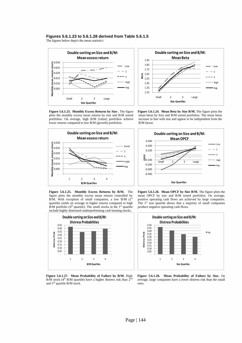
Page | 144
Figures 5.6.1.23 to 5.6.1.28 derived from Table 5.6.1.5 The figures below depict the mean statistics
Figure 5.6.1.23. Monthly Excess Returns by Size . The figure plots the monthly excess mean returns by size and B/M sorted
portfolios. On average, high B/M (value) portfolios achieve
lower returns compared to low B/M (growth) portfolios.
Figure 5.6.1.24. Mean Beta by Size B/M. The figure plots the mean betas by Size and B/M sorted portfolios. The mean betas
increase in line with size and appear to be independent from the
B/M factor.
Figure 5.6.1.25. Monthly Excess Returns by B/M. The
figure plots the monthly excess mean returns controlled by B/M. With exception of small companies, a low B/M (1st
quartile) yields on average in higher returns compared to high
B/M portfolio (4th quartile). The small stocks in the 1st quartile include highly distressed underperforming cash burning stocks.
Figure 5.6.1.26. Mean OPCF by Size B/M. The figure plots the
mean OPCF by size and B/M sorted portfolios. On average, positive operating cash flows are achieved by large companies.
The 1st size quartile shows that a majority of small companies
produce negative operating cash flows.
Figure 5.6.1.27. Mean Probability of Failure by B/M. High B/M stock (4th B/M quartile) have a higher distress risk than 2nd
and 3rd quartile B/M stock.
Figure 5.6.1.28. Mean Probability of Failure by Size. On average, large companies have a lower distress risk than the small
ones.
-
0.005
0.010
0.015
0.020
0.025
0.030
Small 2 3 Large
Mo
nth
ly m
ea
n e
xce
ss r
etu
rn
Size Quartiles
Double sorting on Size and B/M: Mean excess return
Low
2
3
High
Avg
1.25
1.35
1.45
1.55
1.65
1.75
1.85
1.95
Small 2 3 Large
Be
ta
Size Quartiles
Double sorting on Size and B/M: Mean Beta
Low
2
3
High
Avg
-
0.005
0.010
0.015
0.020
0.025
0.030
1 2 3 4
Mo
nth
ly m
ea
n e
xce
ss r
etu
rn
B/M Quartiles
Double sorting on Size and B/M: Mean excess return
Small
2
3
Large
Avg
-0.400
-0.300
-0.200
-0.100
-
0.100
0.200
0.300
Small 2 3 Large
OP
CF
Size Quartiles
Double sorting on Size and B/M: Mean OPCF
Low
2
3
High
Avg
-0.05 0.10 0.15 0.20 0.25 0.30 0.35 0.40 0.45
1 2 3 4
Dis
tre
ss P
rob
B/M Quartiles
Double sorting on Size and B/M: Distress Probabilities
-0.05 0.10 0.15 0.20 0.25 0.30 0.35 0.40 0.45 0.50
1 2 3 4
Dis
tre
ss P
rob
Size Quartiles
Double sorting on Size and B/M: Distress Probabilities
Avg
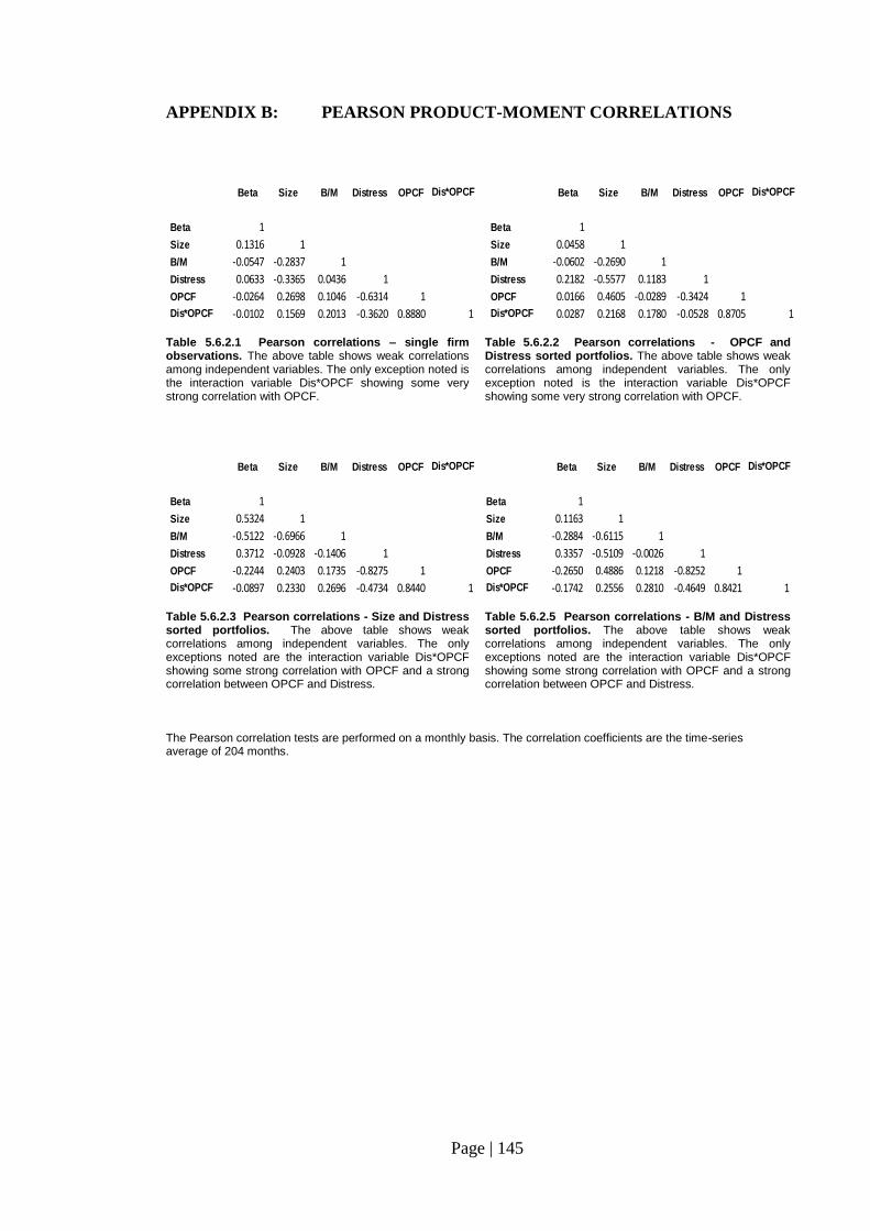
Page | 145
APPENDIX B: PEARSON PRODUCT-MOMENT CORRELATIONS
Table 5.6.2.1 Pearson correlations – single firm observations. The above table shows weak correlations among independent variables. The only exception noted is the interaction variable Dis*OPCF showing some very strong correlation with OPCF.
Table 5.6.2.2 Pearson correlations - OPCF and Distress sorted portfolios. The above table shows weak correlations among independent variables. The only exception noted is the interaction variable Dis*OPCF showing some very strong correlation with OPCF.
Table 5.6.2.3 Pearson correlations - Size and Distress sorted portfolios. The above table shows weak correlations among independent variables. The only exceptions noted are the interaction variable Dis*OPCF showing some strong correlation with OPCF and a strong correlation between OPCF and Distress.
Table 5.6.2.5 Pearson correlations - B/M and Distress sorted portfolios. The above table shows weak correlations among independent variables. The only exceptions noted are the interaction variable Dis*OPCF showing some strong correlation with OPCF and a strong correlation between OPCF and Distress.
The Pearson correlation tests are performed on a monthly basis. The correlation coefficients are the time-series average of 204 months.
Beta Size B/M Distress OPCF Dis*OPCF
Beta 1
Size 0.1316 1
B/M -0.0547 -0.2837 1
Distress 0.0633 -0.3365 0.0436 1
OPCF -0.0264 0.2698 0.1046 -0.6314 1
Dis*OPCF -0.0102 0.1569 0.2013 -0.3620 0.8880 1
Beta Size B/M Distress OPCF Dis*OPCF
Beta 1
Size 0.0458 1
B/M -0.0602 -0.2690 1
Distress 0.2182 -0.5577 0.1183 1
OPCF 0.0166 0.4605 -0.0289 -0.3424 1
Dis*OPCF 0.0287 0.2168 0.1780 -0.0528 0.8705 1
Beta Size B/M Distress OPCF Dis*OPCF
Beta 1
Size 0.5324 1
B/M -0.5122 -0.6966 1
Distress 0.3712 -0.0928 -0.1406 1
OPCF -0.2244 0.2403 0.1735 -0.8275 1
Dis*OPCF -0.0897 0.2330 0.2696 -0.4734 0.8440 1
Beta Size B/M Distress OPCF Dis*OPCF
Beta 1
Size 0.1163 1
B/M -0.2884 -0.6115 1
Distress 0.3357 -0.5109 -0.0026 1
OPCF -0.2650 0.4886 0.1218 -0.8252 1
Dis*OPCF -0.1742 0.2556 0.2810 -0.4649 0.8421 1
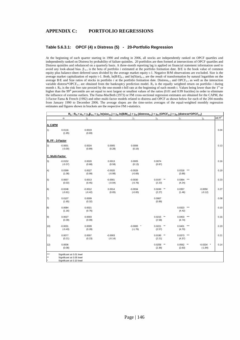
Page | 146
APPENDIX C: PORTFOLIO REGRESSIONS
Table 5.6.3.1: OPCF (4) x Distress (5) - 20-Portfolio Regression
At the beginning of each quarter starting in 1990 and ending in 2006, all stocks are independently ranked on OPCF quartiles and
independently ranked on Distress by probability of failure quintiles. 20 portfolios are then formed at intersections of OPCF quartiles and
Distress quintiles and rebalanced on a quarterly basis. A three-month reporting lag is applied on financial statement information used to avoid any look-ahead bias. β it-1 is the beta of portfolio i estimated at the portfolio formation date. B/E is the book value of common
equity plus balance-sheet deferred taxes divided by the average market equity t-1. Negative B/M observations are excluded. Size is the
average market capitalization of equity t-1. Both, ln(B/E)it-1 and ln(Size)it-1, are the result of transformation by natural logarithm on the average B/E and Size ratios of stocks in portfolio i at the portfolio formation date. Distressit-1 and OPCFit-1 as well as the interaction
variable distress*OPCFit-1 are obtained from the bankruptcy prediction model. Rit is the equally weighted return on portfolio i during
month t. RFt is the risk free rate proxied by the one-month t-bill rate at the beginning of each month t. Values being lower than the 1st or higher than the 99th percentile are set equal to next largest or smallest values of the ratios (0.01 and 0.99 fractiles) in order to eliminate
the influence of extreme outliers. The Fama-MacBeth (1973) or FM cross-sectional regression estimates are obtained for the CAPM, the
3-Factor Fama & French (1992) and other multi-factor models related to distress and OPCF as shown below for each of the 204 months from January 1990 to December 2006. The average slopes are the time-series averages of the equal-weighted monthly regression
estimates and figures shown in brackets are the respective FM t-statistics.
1 2 3 4 5 6 adj R2
A. CAPM
1) 0.0116 0.0019 0.04
(1.65) (0.69)
B. FF - 3-Factor
2) -0.0001 0.0024 0.0005 0.0006 0.13
(-0.00) (0.89) (0.28) (0.16)
C. Multi-Factor
3) -0.0152 0.0020 0.0013 0.0005 0.0074 0.16
(-0.37) (0.68) (0.59) (0.13) (0.87)
4) 0.0399 0.0027 -0.0020 -0.0026 0.0318 *** 0.19
(1.08) (0.99) (-0.99) (-0.69) (3.89)
5) 0.0007 0.0013 -0.0001 -0.0030 0.0197 ** 0.0364 *** 0.23
(0.02) (0.45) (-0.04) (-0.76) (2.22) (4.24)
6) -0.0248 -0.0012 0.0014 -0.0034 0.0249 ** 0.0357 -0.0050 0.27
(-0.61) (-0.42) (0.65) (-0.65) (2.27) (1.46) (-0.12)
7) 0.0107 0.0009 0.0067 0.08
(1.65) (0.32) (0.89)
8) 0.0084 0.0021 0.0323 *** 0.10
(1.16) (0.76) (4.42)
9) 0.0027 0.0003 0.0215 ** 0.0403 *** 0.16
(0.39) (0.09) (2.58) (4.74)
10) -0.0031 0.0009 -0.0065 * 0.0221 ** 0.0401 *** 0.19
(-0.43) (0.28) (-1.76) (2.57) (4.70)
11) 0.0077 0.0007 -0.0003 0.0190 ** 0.0373 *** 0.21
(0.21) (0.23) (-0.14) (2.21) (4.37)
12) 0.0006 0.0258 ** 0.0562 ** -0.0334 * 0.14
(0.08) (2.36) (2.63) (-1.84)
*** Significant at 0.01 level
** Significant at 0.05 level
* Significant at 0.10 level
Rit - RFt = it + 1tit-1 + 2t ln(sizeit-1) + 3t ln(B/Mit-1) + 4t (distressit-1) + 5t (OPCFit-1) + 6t (distress*OPCFit-1)
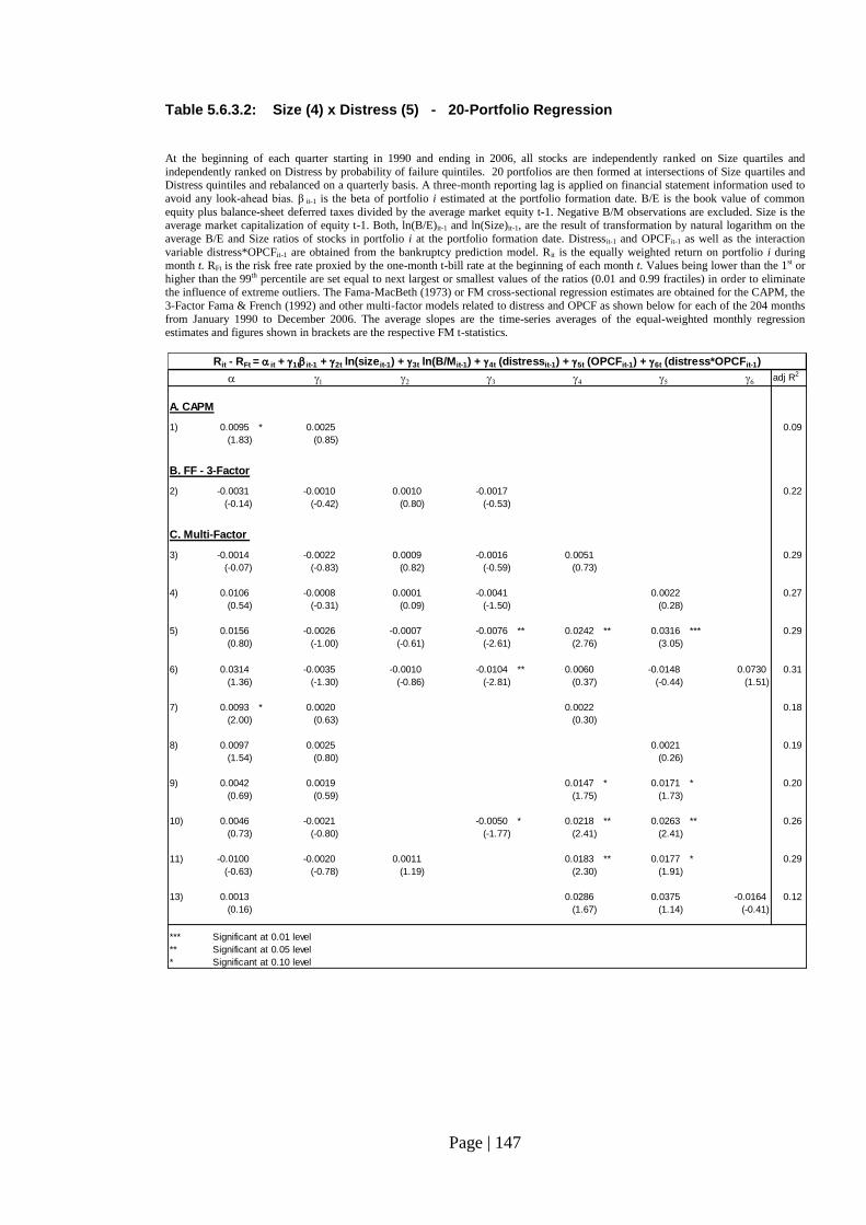
Page | 147
Table 5.6.3.2: Size (4) x Distress (5) - 20-Portfolio Regression At the beginning of each quarter starting in 1990 and ending in 2006, all stocks are independently ranked on Size quartiles and
independently ranked on Distress by probability of failure quintiles. 20 portfolios are then formed at intersections of Size quartiles and Distress quintiles and rebalanced on a quarterly basis. A three-month reporting lag is applied on financial statement information used to
avoid any look-ahead bias. β it-1 is the beta of portfolio i estimated at the portfolio formation date. B/E is the book value of common
equity plus balance-sheet deferred taxes divided by the average market equity t-1. Negative B/M observations are excluded. Size is the average market capitalization of equity t-1. Both, ln(B/E)it-1 and ln(Size)it-1, are the result of transformation by natural logarithm on the
average B/E and Size ratios of stocks in portfolio i at the portfolio formation date. Distressit-1 and OPCFit-1 as well as the interaction
variable distress*OPCFit-1 are obtained from the bankruptcy prediction model. Rit is the equally weighted return on portfolio i during month t. RFt is the risk free rate proxied by the one-month t-bill rate at the beginning of each month t. Values being lower than the 1st or
higher than the 99th percentile are set equal to next largest or smallest values of the ratios (0.01 and 0.99 fractiles) in order to eliminate the influence of extreme outliers. The Fama-MacBeth (1973) or FM cross-sectional regression estimates are obtained for the CAPM, the
3-Factor Fama & French (1992) and other multi-factor models related to distress and OPCF as shown below for each of the 204 months
from January 1990 to December 2006. The average slopes are the time-series averages of the equal-weighted monthly regression
estimates and figures shown in brackets are the respective FM t-statistics.
1 2 3 4 5 6 adj R2
A. CAPM
1) 0.0095 * 0.0025 0.09
(1.83) (0.85)
B. FF - 3-Factor
2) -0.0031 -0.0010 0.0010 -0.0017 0.22
(-0.14) (-0.42) (0.80) (-0.53)
C. Multi-Factor
3) -0.0014 -0.0022 0.0009 -0.0016 0.0051 0.29
(-0.07) (-0.83) (0.82) (-0.59) (0.73)
4) 0.0106 -0.0008 0.0001 -0.0041 0.0022 0.27
(0.54) (-0.31) (0.09) (-1.50) (0.28)
5) 0.0156 -0.0026 -0.0007 -0.0076 ** 0.0242 ** 0.0316 *** 0.29
(0.80) (-1.00) (-0.61) (-2.61) (2.76) (3.05)
6) 0.0314 -0.0035 -0.0010 -0.0104 ** 0.0060 -0.0148 0.0730 0.31
(1.36) (-1.30) (-0.86) (-2.81) (0.37) (-0.44) (1.51)
7) 0.0093 * 0.0020 0.0022 0.18
(2.00) (0.63) (0.30)
8) 0.0097 0.0025 0.0021 0.19
(1.54) (0.80) (0.26)
9) 0.0042 0.0019 0.0147 * 0.0171 * 0.20
(0.69) (0.59) (1.75) (1.73)
10) 0.0046 -0.0021 -0.0050 * 0.0218 ** 0.0263 ** 0.26
(0.73) (-0.80) (-1.77) (2.41) (2.41)
11) -0.0100 -0.0020 0.0011 0.0183 ** 0.0177 * 0.29
(-0.63) (-0.78) (1.19) (2.30) (1.91)
13) 0.0013 0.0286 0.0375 -0.0164 0.12
(0.16) (1.67) (1.14) (-0.41)
*** Significant at 0.01 level
** Significant at 0.05 level
* Significant at 0.10 level
Rit - RFt = it + 1tit-1 + 2t ln(sizeit-1) + 3t ln(B/Mit-1) + 4t (distressit-1) + 5t (OPCFit-1) + 6t (distress*OPCFit-1)
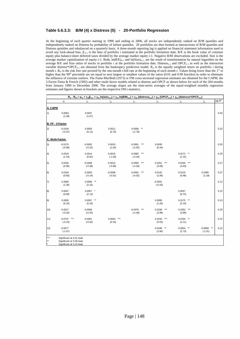
Page | 148
Table 5.6.3.3: B/M (4) x Distress (5) - 20-Portfolio Regression
At the beginning of each quarter starting in 1990 and ending in 2006, all stocks are independently ranked on B/M quartiles and
independently ranked on Distress by probability of failure quintiles. 20 portfolios are then formed at intersections of B/M quartiles and
Distress quintiles and rebalanced on a quarterly basis. A three-month reporting lag is applied on financial statement information used to avoid any look-ahead bias. β it-1 is the beta of portfolio i estimated at the portfolio formation date. B/E is the book value of common
equity plus balance-sheet deferred taxes divided by the average market equity t-1. Negative B/M observations are excluded. Size is the
average market capitalization of equity t-1. Both, ln(B/E)it-1 and ln(Size)it-1, are the result of transformation by natural logarithm on the average B/E and Size ratios of stocks in portfolio i at the portfolio formation date. Distressit-1 and OPCFit-1 as well as the interaction
variable distress*OPCFit-1 are obtained from the bankruptcy prediction model. Rit is the equally weighted return on portfolio i during
month t. RFt is the risk free rate proxied by the one-month t-bill rate at the beginning of each month t. Values being lower than the 1st or higher than the 99th percentile are set equal to next largest or smallest values of the ratios (0.01 and 0.99 fractiles) in order to eliminate
the influence of extreme outliers. The Fama-MacBeth (1973) or FM cross-sectional regression estimates are obtained for the CAPM, the
3-Factor Fama & French (1992) and other multi-factor models related to distress and OPCF as shown below for each of the 204 months from January 1990 to December 2006. The average slopes are the time-series averages of the equal-weighted monthly regression
estimates and figures shown in brackets are the respective FM t-statistics.
1 2 3 4 5 6 adj R2
A. CAPM
1) 0.0063 0.0047 0.03
(1.28) (1.67)
B. FF - 3-Factor
2) -0.0104 0.0003 0.0011 -0.0056 ** 0.22
(-0.37) (0.12) (0.70) (-2.78)
C. Multi-Factor
3) -0.0175 -0.0002 0.0015 -0.0051 *** 0.0030 0.25
(-0.68) (-0.10) (1.04) (-2.92) (0.44)
4) 0.0316 0.0014 -0.0015 -0.0082 *** 0.0172 ** 0.25
(1.24) (0.62) (-1.00) (-4.04) (2.15)
5) 0.0235 -0.0009 -0.0014 -0.0093 *** 0.0251 *** 0.0434 *** 0.27
(0.90) (-0.38) (-0.96) (-4.26) (3.09) (4.63)
6) 0.0164 -0.0003 -0.0008 -0.0091 *** 0.0142 0.0119 0.0380 0.27
(0.60) (-0.14) (-0.51) (-4.02) (1.06) (0.48) (1.18)
7) 0.0060 0.0056 ** -0.0031 0.12
(1.35) (2.15) (-0.43)
8) 0.0047 0.0057 * 0.0057 0.12
(0.80) (2.13) (0.72)
9) 0.0005 0.0057 ** 0.0090 0.0175 ** 0.13
(0.10) (2.16) (1.20) (2.10)
10) -0.0017 -0.0006 -0.0076 *** 0.0236 *** 0.0352 *** 0.25
(-0.32) (-0.25) (-4.48) (2.89) (3.99)
11) -0.0737 *** -0.0001 0.0043 *** 0.0233 *** 0.0164 ** 0.22
(-3.23) (-0.02) (3.32) (3.02) (2.11)
12) -0.0077 0.0436 ** 0.0824 ** -0.0858 ** 0.12
(-1.07) (2.66) (2.73) (-2.31)
*** Significant at 0.01 level
** Significant at 0.05 level
* Significant at 0.10 level
Rit - RFt = it + 1tit-1 + 2t ln(sizeit-1) + 3t ln(B/Mit-1) + 4t (distressit-1) + 5t (OPCFit-1) + 6t (distress*OPCFit-1)
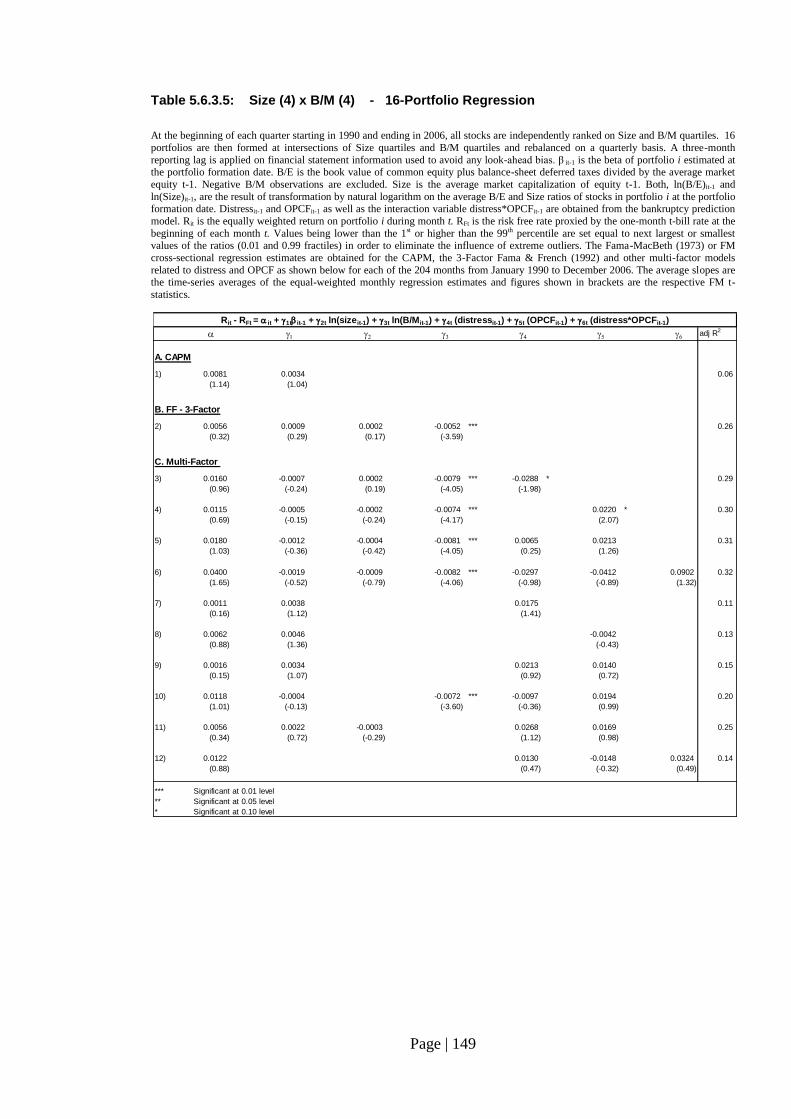
Page | 149
Table 5.6.3.5: Size (4) x B/M (4) - 16-Portfolio Regression
At the beginning of each quarter starting in 1990 and ending in 2006, all stocks are independently ranked on Size and B/M quartiles. 16
portfolios are then formed at intersections of Size quartiles and B/M quartiles and rebalanced on a quarterly basis. A three-month
reporting lag is applied on financial statement information used to avoid any look-ahead bias. β it-1 is the beta of portfolio i estimated at the portfolio formation date. B/E is the book value of common equity plus balance-sheet deferred taxes divided by the average market
equity t-1. Negative B/M observations are excluded. Size is the average market capitalization of equity t-1. Both, ln(B/E)it-1 and
ln(Size)it-1, are the result of transformation by natural logarithm on the average B/E and Size ratios of stocks in portfolio i at the portfolio formation date. Distressit-1 and OPCFit-1 as well as the interaction variable distress*OPCFit-1 are obtained from the bankruptcy prediction
model. Rit is the equally weighted return on portfolio i during month t. RFt is the risk free rate proxied by the one-month t-bill rate at the
beginning of each month t. Values being lower than the 1st or higher than the 99th percentile are set equal to next largest or smallest values of the ratios (0.01 and 0.99 fractiles) in order to eliminate the influence of extreme outliers. The Fama-MacBeth (1973) or FM
cross-sectional regression estimates are obtained for the CAPM, the 3-Factor Fama & French (1992) and other multi-factor models
related to distress and OPCF as shown below for each of the 204 months from January 1990 to December 2006. The average slopes are the time-series averages of the equal-weighted monthly regression estimates and figures shown in brackets are the respective FM t-
statistics.
1 2 3 4 5 6 adj R2
A. CAPM
1) 0.0081 0.0034 0.06
(1.14) (1.04)
B. FF - 3-Factor
2) 0.0056 0.0009 0.0002 -0.0052 *** 0.26
(0.32) (0.29) (0.17) (-3.59)
C. Multi-Factor
3) 0.0160 -0.0007 0.0002 -0.0079 *** -0.0288 * 0.29
(0.96) (-0.24) (0.19) (-4.05) (-1.98)
4) 0.0115 -0.0005 -0.0002 -0.0074 *** 0.0220 * 0.30
(0.69) (-0.15) (-0.24) (-4.17) (2.07)
5) 0.0180 -0.0012 -0.0004 -0.0081 *** 0.0065 0.0213 0.31
(1.03) (-0.36) (-0.42) (-4.05) (0.25) (1.26)
6) 0.0400 -0.0019 -0.0009 -0.0082 *** -0.0297 -0.0412 0.0902 0.32
(1.65) (-0.52) (-0.79) (-4.06) (-0.98) (-0.89) (1.32)
7) 0.0011 0.0038 0.0175 0.11
(0.16) (1.12) (1.41)
8) 0.0062 0.0046 -0.0042 0.13
(0.88) (1.36) (-0.43)
9) 0.0016 0.0034 0.0213 0.0140 0.15
(0.15) (1.07) (0.92) (0.72)
10) 0.0118 -0.0004 -0.0072 *** -0.0097 0.0194 0.20
(1.01) (-0.13) (-3.60) (-0.36) (0.99)
11) 0.0056 0.0022 -0.0003 0.0268 0.0169 0.25
(0.34) (0.72) (-0.29) (1.12) (0.98)
12) 0.0122 0.0130 -0.0148 0.0324 0.14
(0.88) (0.47) (-0.32) (0.49)
*** Significant at 0.01 level
** Significant at 0.05 level
* Significant at 0.10 level
Rit - RFt = it + 1tit-1 + 2t ln(sizeit-1) + 3t ln(B/Mit-1) + 4t (distressit-1) + 5t (OPCFit-1) + 6t (distress*OPCFit-1)
Page | 150
REFERENCES
AGARWAL, V., TAFFLER, R., 2008, Does Financial Distress Risk Drive the Momentum Anomaly? Financial
Management, Autumn 2008, 461 – 484
AGARWAL, V., TAFFLER, R., 2008, Comparing the Performance of Market-Based and Accounting-Based Bankruptcy
Prediction Models”. Journal of Banking & Finance, 32, 1541 – 1551
ALFORD, A.W., JONES, J.J., ZMIJEWSKI, M., 1994, Extensions and Violations of the Statutory 10-K Filing
Requirements. Journal of Accounting and Economics, 17, 229 – 254
ALTMAN, E.I., 1968, Financial Ratios, Discriminant Analysis and the Prediction of Corporate Bankruptcy. The
Journal of Finance, September, 589 – 609
ALTMAN, E.I., BRENNER, M., 1981, Information Effects and Stock Market Response to Signs of Firm Deterioration.
Journal of Financial and Quantitative Analysis, March, 35 – 51
ALTMAN, E.I., EISENBEIS, R.A., 1978, Financial Applications of Discriminant Analysis: A Clarification. Journal of
Financial and Quantitative Analysis, March, 185 – 195
ALTMAN, E.I., HALDEMAN, R.G., NARAYAN, P., 1977, Zeta Analysis: A New Model to Identify Bankruptcy Risk of
Corporation. Journal of Banking and Finance, Vol. 1, Nr. 1, 29 - 51
ALTMAN, E.I., 1993, Corporate Financial Distress and Bankruptcy. New York: John Wiley & Sons, Inc.
AMRHEIN D.G., KATZ, J.A., 1998, Cash Flow as a Factor in the Mortality Risk of Business. International Council for
Small Business, Singapore Conference Proceedings, No. 18
AZIZ, A., EMANUEL, D., LAWSON, G.H., 1988, Bankruptcy Prediction – An Investigation of Cash Flow Based
Models. Journal of Management Studies, 25:5, 419 – 437
BALCAEN, S., OOGHE, H., 2006, 35 Years of Studies on Business Failure: An Overview of the Classical Statistical
Methodologies and their Related Problems. The British Accounting Review 38, 63–93
BALL, R., BROWN, P. 1968, An Empirical Evaluation of Accounting Income Numbers. Journal of Accounting Research,
Autumn, 159 – 178
BALL, R., 1978, Anomalies in Relationships between Securities' Yields and Yield-surrogates. Journal of Financial
Economics 6, 103 – 126
BANZ, R.W., 1981, The Relationship between Return and Market Value of Common Stocks. Journal of Financial
Economics 9, 3 – 18
BANZ, R.W., BREEN, W.J., 1986, Sample-Dependent Results using Accounting and Market Data: Some Evidence.
Journal of Finance 41, 779 – 793
BASU, S., 1983, The Relationship between Earnings Yield, Market Value, and Return for NYSE Common Stocks:
Further evidence. Journal of Financial Economics 12, 129 – 156
BARBERIS, N., HUANG M., 2008, Stock as Lotteries: The Implications of Probability Weighting for Security Prices.
American Economic Review 98, 2066 – 2100
BARNES, P., 1982, Methodological Implications of Non-normality Distributed Financial Ratios. Journal of Business
Finance and Accounting, Vol. 9, No. 1, Spring, 51 – 62
BEGLEY, J., MING J., WATTS, S., 1996, Bankruptcy Classification Errors in the 1980s: An Empirical Analysis of
Altman’s and Ohlson’s Models, Review of Accounting Studies 1, 267 – 284
BEAVER, W., 1966, Financial Ratios as Predictors of Failure, Empirical Research in Accounting: Selected Studies.
supplement to vol. 5, Journal of Accounting Research, 71 – 111
BEAVER, W., 1968, Market Prices, Financial Ratios and the Prediction of Failure. Journal of Accounting Research,
Autumn, 179 – 199
BEAVER, W., 1998, Financial Reporting: An Accounting Revolution. Third edition. Upper Saddle, NJ: Prentice
Hall.
Page | 151
BEAVER, W., MCNICHOLS, M. F., RHIE, J-W., 2004, Have Financial Statements Become Less Informative? Evidence
from the Ability of Financial Ratios to Predict Bankruptcy. Working Paper, Stanford University
BLACK, F., 1972, Capital Market Equilibrium with Restricted Borrowing. Journal of Business, 45, 444 – 455
BLACK F., JENSEN, M.C., SCHOLES, M., 1971. The Capital Asset Pricing Model: Some
Empirical Tests. in: M. Jensen. ed.. Studies In the theory of capital markets (Praeger, New York, NY)
BLACK, F., 1993, Beta and Return. Journal of Portfolio Management, 20, 8 – 18
BLUM, M., 1974, Failing Company Discriminant Analysis. Journal of Accounting Research, Spring 1974, 1-25
CAMPELL, J.Y., HILSCHER J., SZILAGYI, J., 2008, In Search of Distress Risk. The Journal of Finance, 6, 2899 –
2939
CLEVES, M.A., GOULD, W.W., GUTIERREZ R.G., 2003, An Introduction to Survival Analysis using STATA. STATA
Press
CHAN, K.C., HAMAO Y., LAKONISHOK J., 1991, Fundamentals and Stock Returns in Japan. Journal of Finance 46,
1739 – 1789
CHAN, K.C., CHEN, N., 1991, Structural and Return Characteristics of Small and Large Firms. Journal of Finance, 46,
1467 -1484
CHAN, K.C., JEGADEESH, N., LAKONISHOK, J., 1995, Evaluating the Performance of Value versus Glamour Stocks:
The Impact of Selection Bias. Journal of Financial Economics 38, 269 – 296
CHARITOU, A., CLUBB, C., 1999., Earnings, Cash Flow and Security Returns over Long Return Intervals: Analysis
and UK Evidence. Journal of Business Finance and Accounting, 26 (3)(4), 283 – 312
CHAVA, S., JARROW, R., 2004, Bankruptcy Prediction with Industry Effects. Review of Finance, 8, 537 – 569
CHOPRA, N., LAKONISHOK, J., RITTER, JL, 1992, Measuring Abnormal Performance: Do Stocks Overreact?
Journal of Financial Economics 31, 235 – 268
COCHRANE, J.H., 2005, Asset Pricing. Revised Edition. Princeton and Oxford. Princeton University Press
COHEN, R.B., GOMPERS, P.A., VUOLTEENAHO, T., 2002, Who underreacts to Cash-Flow News? Evidence from
Trading between Individuals and Institutions. Journal of Financial Economics 66, 409 – 462
COX, D.Rl, 1972, Regression Models and Life-Tables (with Discussion). Journal of the Royal Statistical Society, Series
B 34, 187 – 220
DEAKIN, E., 1972, A Discriminant Analysis of Predictors of Business Failure. Journal of Accounting Research, Spring,
167 – 179
DECHOW, P.M., 1994, Accounting Earnings and Cash Flows as Measures of Firm Performance. The Role of
Accounting Accruals. Journal of Accounting and Economics, 18, 3 – 42
DIAMOND, H. JR., 1976, Pattern Recognition and the Detection of Corporate Failure. Ph.D. dissertation, New York
University
DICHEV, I., 1998, Is the Risk of Bankruptcy a Systematic Risk?. The Journal of Finance, Vol III, No 3, 1131 - 1147
DIETRICH, J.R., 1984, Discussion of Methodological Issues Related to the Estimation of Financial Distress Prediction
Models. Journal of Accounting Research, Vol. 22 Supplement, 83 – 86
EASTON, P.D., ZMIJEWSKI, M.E., 1989, Cross-sectional Variation in the Stock Market Response to Accounting
Earnings Announcements. Journal of Accounting and Economics, Vol. 11, 117 – 141
EASTON, P.D., HARRIS, T.S., 1991, Earnings as an Explanatory Variable for Returns. Journal of Accounting Research,
Spring, 19 – 36
EDMISTER, R., 1972, An Empirical Test of Financial Ratio Analysis for Small Business Failure Prediction. Journal of
Financial and Quantitative Analysis, 1477 – 1493
ENGELMANN, B., HAYDEN, E., TASCHE, D., Testing Rating Accuracy. Risk 16, 82 – 86
Page | 152
EISENBEIS, R.A., 1977, Pitfalls in the Application of Discriminant Analysis in Business. Journal of Finance, Vol. 32,
No. 3, 875 – 900
FAMA, E.F.., FRENCH, K.R., 1992, The Cross-Section of Expected Stock Returns. Journal of Finance, 2, 427 - 465
FAMA, E.F., FRENCH, K.R., 1993, Common Risk Factors in the Returns on Stocks and Bonds. Journal of Financial
Economics, 33, 3 – 56
FAMA, E.F., FRENCH, K.R., 1995, Size and Book-to-Market Factors in Earnings and Returns. Journal of Finance, 50,
131 – 155
FAMA, E.F., FRENCH, K.R., 1996, Multifactor Explanations of Asset Pricing Anomalies. Journal of Finance, 51, 55 –
84
FAMA, E.F., FRENCH, K.R., 1997, Industry Costs of Equity. Journal of Financial Economics 43, 153 – 193
FAMA, E.F., FRENCH, K.R., 2006, Profitability, Investment and Average Returns. Journal of Financial Economics, 82,
491 – 518
FAMA, E.F., MACBETH J.D., 1973, Risk, Return and Equilibrium: Empirical Tests. Journal of Political Economy, 81,
607 – 636
FERGUSON, M.F., SHOCKLEY, R.L., 2003, Equilibrium Anomalies. Journal of Finance 58, 2549 – 2580
FRECKA, T.J., HOPWOOD, W.S., 1983, The Effects of Outliers on the Cross-Sectional Distributional Properties of
Financial Ratios, The Accounting Review 58, 115 – 128
GRAMBESCH, P.M., THERNEAU, T.M., 1994, Proportional Hazard Tests and Diagnostics based on Weighted
Residuals. Biometrika 81, 515 – 526
GRICE J.S., INGRAM R.W.., 2001, Tests of the generalizability of Altman’s bankruptcy prediction model, Journal of
Business Research 54, 53 – 61
GRIFFIN, J., LEMMON, L., 2002, Book-to-Market Equity, Distress Risk and Stock Returns. Journal of Finance 57, 2317
– 2336
HANLEY, J., MCNEIL, B., 1982, The Meaning and Use of the Area Under a Receiver Operating Characteristic (ROC)
Curve. Radiology 143 (1), 29 – 36
HANLEY, J., MCNEIL, B., 1983, A Method of Comparing the Areas Under Receiver Operating Characteristic Curves
Derived from the Same Cases. Radiology 148 (3), 839 – 843
HAUGEN, R.A., 1995, The New Finance – The Case against Efficient Markets. (Prentice-Hall, Englewood Cliffs, NJ).
HAUGEN, R.A., BAKER, N.L., 1996, Commonality in the Determinants of Expected Stock Returns. Journal of Financial
Economics 41, 401 – 439
HILLMER, S.C., YU, P.L., 1979, The Market Speed of Adjustment to New Information. Journal of Financial Economics
7, December, 321 – 345
HOROWITZ, J.L., LOUGHRAN, T., SAVIN, N.E., 2000, The Disappearing Size Effect. Research in Economics 54,
2143 – 2184
KARELS, G.V., PRAKASH, A.J., 1987, Multivariate Normality and Forecasting of Business Bankruptcy. Journal of
Business and Accounting, 14(4) Winter, 573 – 593
KIEFER, N.M., 1988, Economic Duration Data and Hazard Functions. Journal of Economic Literature 26, 646 - 679
KOTHARI, S.P., 2001, Capital Markets Research in Accounting. Journal of Accounting and Economics 31, 105 – 231
KOTHARI, S.P., SHANKEN J., SLOAN R.G., 1995, Another Look at the Cross-Section of Expected Returns. Journal of
Finance 50, 185 – 224
KOVTUNENKO, B. SOSNER, N., 2003, Sources of Institutional Performance. Working Paper, Harvard University
LACHENBRUCH, P.A., 1975, Discriminant Analysis. New York: Hafner Press
Page | 153
LAKONISHOK, J. SHAPIRO, A.C., 1986, Systematic Risk, Total Risk and Size as Determinants of Stock Market
Returns. Journal of Banking and Finance 10, 115 – 132
LAKONISHOK, J., SHLEIFER, A., VISHNY, R., 1994, Contrarian Investment, Extrapolation and Risk. Journal of
Finance 49, 1541 – 1578
LANE, W.R., LOONEY, S.W., WANSLEY, J.W., 1986. An application of the Cox proportional hazards model to bank
failure. Journal of Banking and Finance 10, 511–531.
LAWSON, G.H., 1971. Accounting for Financial Management: some Tentative Proposals for a new Blueprint. In Shone,
R. (Ed.), Problems of Investment. Oxford: Blackwell
LINTNER, J., 1965a,. Security Prices, Risk and Maximal Gains from Diversification. Journal of Finance, 20, 587 – 615
LINTNER, J., 1965b,. The valuation of Risky Investments in Stock Portfolios and Capital Budgets. Review of
Economics and Statistics, 47, 13 – 37
LO, A.W., MACKINLAY, A.C., 1990,. Data Snooping in Tests of Financial Asset Pricing Models. Review of Financial
Studies, 10, 431 – 467
LOUGHRAN, T., 1997, Book-to-Market across Firms Size and Seasonality: Is there an Effect? Journal of Financial and
Quantitative Analysis 32, 249 – 268
JONES F.L., 1987,. Current Techniques in Bankruptcy Prediction. Journal of Accounting Literature, 6, 131 – 164
JOY, M.O., TOLLEFSON, J.O., 1975, On the Financial Applications of Discriminant Analysis. Journal of Financial and
Quantitative Analysis, 723 – 739
MACKINLAY, A.C., 1995,. Multifactor Models do not explain Deviations from the CAPM. Journal of Financial
Economics, 38, 3 – 28
MCLEAY, S., OMAR, A., 2000, The Sensitivity of Prediction Models to the Non-Normality of Bounded and unbounded
Financial Ratios. British Accounting Review, Vol 32, 213 – 230
MENSAH, Y.M., 1984, An Examination of the Stationarity of Multivariate Bankruptcy Prediction Models: A
Methodological Study. Journal of Accounting Research, Vol. 22, No 1, 380 – 395
MERTON, R.C., 1971, Optimal Consumption and Portfolio Rules in a Continuous-Time Model. Journal of Economic
Theory, 3, 373 – 413
MERTON, R.C., 1972, An Analytic Derivation of the Efficient Frontier. Journal of Financial and Quantitative Analysis, 7,
1851 – 1872
MERTON, R.C., 1973, An Intertemporal Capital Asset Pricing Model. Econometrica, 41, 867 – 887
MOSSIN, J., 1966, Equilibrium in a Capital Asset Market. Econometrica, 34, 768 – 783
OHLSON, J., 1980, Financial Ratios and the Probabilistic Prediction of Bankruptcy. Journal of Accounting Research,
Spring, 109 – 131
OHLSON, J.A., SHROFF, P.K., 1992. Changes versus Levels in Earnings as Explanatory Variables for Returns: Some
Theoretical Considerations. Journal of Accounting Research, Vol. 30 No. 2, 210 – 226
PENMAN, S.H., 1987, The Distribution of Earnings News over Time and Seasonalities in Aggregate Stock Returns.
Journal of Financial Economics 18, 199 – 228
PENMAN, S.H., 1992, Return to Fundamentals. Journal of Accounting, Auditing & Finance, Vol. 7, 465 – 483
PLATT, H.D., PLATT, M.B., 1990, Development of a Class of Stable Predictive Variables: The Case of Bankruptcy
Prediction. Journal of Business Finance & Accounting, 17(1) Spring, 33- 51
PLATT, H.D., PLATT, M.B., 1991, A Note on the Use of Industry-relative Ratios in Bankruptcy Prediction. Journal of
Banking and Finance, 15, 1183 – 1194
PLATT, H.D., PLATT, M.B., 2002, Predicting Corporate Financial Distress: Reflections on Choice-based sample bias.
Journal of Economics and Finance, Vol. 26, 184 – 199
Page | 154
POMPE, P., BILDERBEEK, J., 2000, Faillissementspredictie: Een Vergelijiking tussen Lineaire Discriminant Analyse
en Neurale Netwerken. Economisch Sociaal Tijdschrift, Vol.2, 215 – 242
PRICEWATERHOUSECOOPERS LLP., 2006, The Phoenix Report: A Study of Bankruptcies 2005-2006.
PricewaterhouseCoopers LLP, PwC Advisory and Crisis Management
RICHARDSON, F.M., DAVIDSON, L.F., 1984, On Linear Discrimination with Accounting Ratios. Journal of Business
Finance & Accounting, 11(4) Winter, 511 – 525
ROLL, R., 1977, A Critique of the Asset Pricing Theory's Tests Part I: On Past and Potential Testability of the Theory.
Journal of Financial Economics 4 (2), 129 – 176
ROSS S.., 1976, The Arbitrage Theory of Capital Asset Pricing. Journal of Economic Theory, 13, 341 – 360
ROSS ST., WESTERFIELD R.W., JAFFE J.F., 2002, Corporate Finance International Edition. McGraw Hill, 6th
Edition
SCHOENFELD, D., 1982, Partial Residuals for the Proportional Hazards Regression Model. Biometrika 69, 239 – 241
SHARPE, W.F., 1964, Capital Asset Prices: A theory of market equilibrium under conditions of risk. Journal of Finance,
19, 425-442
SHUMWAY, T., 2001, Forecasting Bankruptcy More Accurately: A simple Hazard Model. Journal of Business, 74,
101-124
SOBEHART, J., KEENAN, S., STEIN, R., 2000, Benchmarking Quantitative Default Risk Models: A Validation
Methodology. Moody’s Rating Methodology
STRONG, N., 1993, The Relation between Returns and Earnings: Evidence for the UK. Journal of Accounting and
Business Research, Vol. 24, No. 93, 69 – 77
TAFFLER, R.J., TISSHAW, H., 1977, Going, Going, Gone – Four Factors Which Predict. Accountancy, Vol. 88, March,
50 - 54
TAFFLER, R.J., 1983, The Assessment of Company Solvency and Performance using a Statistical Model. Accounting
and Business Research 15(52), 295 – 308
TAFFLER, R.J., 1984, Empirical Models for the Monitoring of UK Corporations. Journal of Banking and Finance 8, 199
– 227
ZAVGREN, C.V., 1983, The Prediction of Corporate Failure: The State of The Art. Journal of Accounting Literature,
Vol. 2., 1 – 37
ZAVGREN, C.V., DUGAN, M.T., REEVE J.M., 1988, The Association between Probabilities of Bankruptcy and Market
Responses – A Test of Market Anticipation. Journal of Business Finance & Accounting, 15(1) Spring, 27 – 45
ZHANG, Y., 2006, Individual Skewness and the Cross-Section of Average Stock Returns, Working Paper, Yale
University
ZMIJEWSKI, M.E., 1984, Methodological Issues Related to the Estimation of Financial Distress Prediction Models.
Journal of Accounting Research, Vol. 22 Supplement, 59 - 82