carlota andrés - cern indico

Carlota Andrés

Fully resummed medium-induced emissions in

dynamic media

CPhT, École Polytechnique QM2022, Krakow, Poland

In collaboration with: L. Apolinario, F. Dominguez, M.G. Martinez, C.A. Salgado

2

Energy loss

• Jet quenching: high energy partons interact with the QGP losing energy

• How does a parton lose energy in a QCD medium?

• Collisions - Important for heavy particles

• Radiation - Extra gluon radiation induced by multiple scatterings with the medium Dominant for light quarks and gluons (this talk)

Carlota Andrés

ω, k

E, p0ω, k

QM2022

E, p0ω, k

• The in-medium spectrum is given by :(ω ≪ E)

The building block

• It has been traditionally evaluated in many approximations (GLV, AMY, HO…)

Caron-Huot and Gale, 1006.2379

Carlota Andrés 3 QM2022

BDMPS-Z

• Several new approaches go beyond the usual approximations

• It’s numerical evaluation is difficult

Finite length rates:

IOE (expansion around the HO):

Fully resummed spectrum: CA, Apolinario, Martinez, Dominguez, 2002.01517, 2011.06522

Mehtar-Tani, Barata, Soto-Ontoso, Tywoniuk, 1903.00506, 2106.07402

Finite length rates + non-perturbative potential: Schlichting, Soudi, 2111.13731

https://arxiv.org/abs/1006.2379






4Carlota Andrés

CA, Martinez, Dominguez, 2011.06522

QM2022

• Numerics done in the brick!

The building block: in the brick

Emission spectrum

Emission rates

10°3 10°2 0.1 1 10 50!/!̄c

0

2

4

6

8

10

12

!dI

med/d

!

n0L = 12.2

Full

HO + NLO

GLV N = 1

Low-! limit

Brick(IOE)

ωdIdω

= ∫L

0dt ω

dΓdωdt

dΓ/d

ωdt


Brick T = 200 MeV

t

ω̄c =μ2L

2



How do we move to a realistic medium?


Carlota Andrés 6

• The goal is to compute the energy lost by a hard parton along its trajectory within an evolving media

Beyond the brick

• Then, obtain the medium parameters entering the spectrum: n(T(t)) , μ(T(t)) . . .

• One should read the medium properties (for instance, the temperature T) from the hydro at each point of the path

• And feed them to the code and compute the spectrum along the trajectory

*with multiple scatterings

t (fm)

Glauber

fKLN

PbPb 2.76 TeV b=2.0 fm

T(M

eV)

The spectrum depends on the full trajectory, there is no “per-point spectrum”

QM2022

Carlota Andrés 7

Beyond the brick II• We can compute the spectrum with time-dependent variables along a path

*with multiple scatterings

• But this is computationally demanding. Currently, it seems too costly to do it for every trajectory on the fly

ω̄c =μ2L

2

nhydro(t) = kT3(t)

• Pre-tabulate it? How do we know a priori how the medium parameters will behave along all possible paths?

QM2022

10°3 10°2 10°1 100 101

!/!̄c

0

2

4

6

!dI

med/d

!

n0L = 5

fKLN x < 1 y < 1

Glauber x < 1 y < 1

Full


t (fm)

Glauber

fKLN


T(M

eV)

nhydro = kT3(t)

8Carlota Andrés

• Using average values

Use a static spectrum whose parameters are given by their average along the path

• Let’s say that along the path:

n(t) =n′ 0

(t + t0)α

• Obtain the full dynamic solution for n(t)

• Compare to the static case where n0L is given by the average of n(t) along the path:

n0L = ∫L

0dt n(t)

Using average values does not work well!** And this is something we know since 2003

ω̄c =μ2L

2

10°2 10°1 100 101

0

1

2

3

4

!dI

med/d

!

n0L = 5

Æ = 1

static

10°2 10°1 100 101

!/!̄c

1.0

1.2

1.4

1.6

rati

o

t0 = 0.1

Full

QM2022

Average values?

constantμ


• The idea is to find an equivalent static scenario

Find the values of the parameters that best approximate the dynamic spectrum along the path

• Example:

- Compute the spectrum for a dynamic media where

- Compare to the static scenario given by

n(t) =n′ 0

(t + t0)α

n0L = ∫L′

0dt n(t)

n0L2

2= ∫

L′

0dt t n(t)

10°2 10°1 100 101

0

1

2

3

4

!dI

med/d

!

n0L = 5

Æ = 1

static

10°2 10°1 100 101

!/!̄c

0.96

1.00

1.04

rati

o

Full

t0 = 0.1

ω̄c =μ2L

2

Scaling laws

Scaling laws similar to these ones have been used in the HO. Salgado, Wiedemann, 0302184

constantμ

Scaling laws?

https://arxiv.org/abs/hep-ph/0302184

Carlota Andrés

n(t) =n′ 0

(t + t0)α

n0L = ∫L′

0dt n(t)

n0μ2L2

2= ∫

L′

0dt t n(t) μ2(t)

• Compute the full dynamic solution using

• Find the values of the parameters of the static scenario we want to compare to:

μ2(t) =μ′

2

(t + t0)2α

10°2 10°1 100 1010

1

2

3

4

5

!dI

med/d

!

Æ = 1

static

10°2 10°1 100 101

!/!̄c

0.8

0.9

1.0ra

tio

n0L = 5t0 = 0.1

Scaling laws?

• It works better than using average values, but the errors go up to ~20%

Full

10

ω̄c =μ2L

2

QM2022

μ2(t)

Carlota Andrés

nhydro(t) = k1T(t)

n0L = ∫L′

0dt nhydro(t)

n0μ2L2

2= ∫

L′

0dt t nhydro(t) μ2

hydro(t)

• Compute the full solution along a path thorough a hydro

• Find the values of the parameters of the static scenario we want to compare to:

μ2hydro(t) = k2T2(t)

Scaling laws? Hydro

• It works better than using average values, but the errors go up to ~20%

11

ω̄c =μ2L

2

QM2022

Hydro: Luzum and Romatschke, 0901.4588

10°2 10°1 100 1010

1

2

3

4

!dI

med/d

!

(n0L)st = 5

PbPb 2.76 TeV b = 2 fm

static

10°2 10°1 100 101

!/!̄c

0.8

0.9

1.0

Full

μ2(t)

t0 = 0.1


Carlota Andrés

Scaling laws w.r.t. a power-law case?

12 QM2022

Goal: find matching relations between the spectrum in the real world (along a path throughout a hydro) and a pre-tabulated power-law spectrum

• Why the pre-tabulated spectrum needs to be the static one?

n(t) =n′ 0

(t + t0)α μ2(t) =μ′

2

(t + t0)2α

• For instance: Compute the spectrum along a path throughout a hydro:

Compare to a power-law spectrum for a profile given by:

• The idea is to find an equivalent scenario given by a power-law

with a scaling law given by

∫L1

0dt n(t) = ∫

L2

0dt nhydro(t)

nhydro(t) = k1T(t) μ2hydro(t) = k2T2(t)

∫L1

0dt t n(t) μ2(t) = ∫

L2

0dt t nhydro(t) μ2

hydro(t)

Carlota Andrés

Scaling laws w.r.t. a power-law case

13

ω̄c =μ2L

2

QM2022

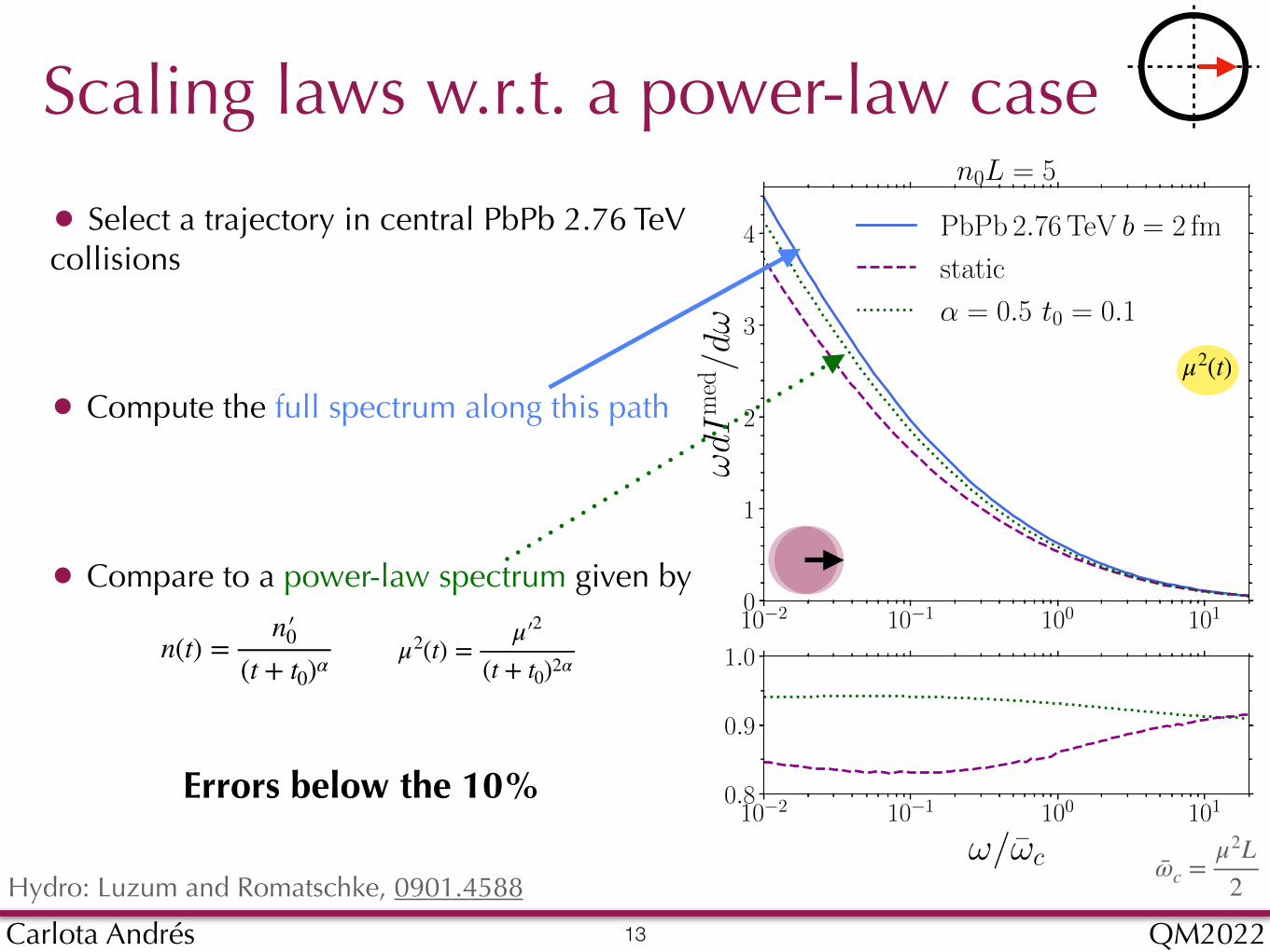
Errors below the 10%

• Select a trajectory in central PbPb 2.76 TeV collisions

• Compute the full spectrum along this path

• Compare to a power-law spectrum given by

n(t) =n′ 0

(t + t0)α μ2(t) =μ′

2

(t + t0)2α


10°2 10°1 100 1010

1

2

3

4

!dI

med/d

!

n0L = 5


static

Æ = 0.5 t0 = 0.1

10°2 10°1 100 101

!/!̄c

0.8

0.9

1.0

μ2(t)


Carlota Andrés


13

ω̄c =μ2L

2

QM2022

Errors below the 10%

• Select a trajectory in central PbPb 2.76 TeV collisions

• Compute the full spectrum along this path


10°2 10°1 100 1010

1

2

3

4

!dI

med/d

!

n0L = 5


static

Æ = 0.5 t0 = 0.1

10°2 10°1 100 101

!/!̄c

0.8

0.9

1.0

μ2(t)

10°2 10°1 100 1010

1

2

3

4

!dI

med/d

!

n0L = 5


static

Æ = 0.5 t0 = 0.1

Æ = 1 t0 = 0.1

10°2 10°1 100 101

!/!̄c

0.8

0.9

1.0

μ2(t)

• Compare to a power-law with α = 0.5

• Compare to a power-law with α = 1


Carlota Andrés


14

ω̄c =μ2L

2QM2022

• PbPb 2.76 TeV 30-40%


• PbPb 2.76 TeV 0-5%

10°2 10°1 100 1010

1

2

3

4

!dI

med/d

!

n0L = 5

PbPb 2.76 TeV b = 2.0 fm µ = 225

static

Æ = 0.5 t0 = 0.1

10°2 10°1 100 101

!/!̄c

0.8

0.9

1.0

μ2(t)

10°2 10°1 100 1010

1

2

3

4

!dI

med/d

!

n0L = 5

PbPb 2.76 TeV b = 8.5 fm µ = 45

static

Æ = 0.5 t0 = 0.1

10°2 10°1 100 101

!/!̄c

0.8

0.9

1.0

μ2(t)μ2(t) μ2(t)


Carlota Andrés


14

ω̄c =μ2L

2QM2022

• PbPb 2.76 TeV 30-40%


• PbPb 2.76 TeV 0-5%

10°2 10°1 100 1010

1

2

3

4

!dI

med/d

!

n0L = 5

PbPb 2.76 TeV b = 2.0 fm µ = 225

static

Æ = 0.5 t0 = 0.1

10°2 10°1 100 101

!/!̄c

0.8

0.9

1.0

μ2(t)

10°2 10°1 100 1010

1

2

3

4

!dI

med/d

!

n0L = 5

PbPb 2.76 TeV b = 8.5 fm µ = 45

static

Æ = 0.5 t0 = 0.1

10°2 10°1 100 101

!/!̄c

0.8

0.9

1.0

μ2(t)

10°2 10°1 100 1010

1

2

3

4

!dI

med/d

!

n0L = 5

PbPb 2.76 TeV b = 2.0 fm µ = 225

static

Æ = 0.5 t0 = 0.1

Æ = 1 t0 = 0.1

10°2 10°1 100 101

!/!̄c

0.8

0.9

1.0

μ2(t)

10°2 10°1 100 1010

1

2

3

4

!dI

med/d

!

n0L = 5

PbPb 2.76 TeV b = 8.5 fm µ = 45

static

Æ = 0.5 t0 = 0.1

Æ = 1 t0 = 0.1

10°2 10°1 100 101

!/!̄c

0.8

0.9

1.0

μ2(t)


Carlota Andrés 15

Conclusions• Many new developments in the computation of the medium-induced radiation

spectrum (in the brick)

• These numerical approaches allow to compute the spectrum along a path in realistic media (given by a hydro)

• So we want to use pre-compute the spectra for a set of given profiles approximating realistic conditions (scaling laws)

• Using power-law profiles reduces the errors substantially

• But it is computationally demanding

Whatever the approach/approximation used, we can quantify the errors!

• We can think of other approachesFor instance, MC approach to mimic the Caron-Huot rates Park et al. HP2016 proceedings 1612.06754


Thanks


10°3 10°2 10°1 100 101

!/!̄c

2

4

6

8

10

12

!dI

med/d

!

µ variable

(n0L)st = 10 µ2(t) = T 2(t) n(t) = T (t)

static

fKLNb2.0 x < 1 y < 1

Æ = 0.5 t0 = 0.1

10°3 10°2 10°1 100 101

!/!̄c

2

4

6

!dI

med/d

!

µ variable

(n0L)st = 5 µ2(t) = T 2(t) n(t) = T (t)

static

fKLNb2.0 x < 1 y < 1

Æ = 0.5 t0 = 0.1

T(t) =T0

(t + t0)α

10°2 100 102

0

1

2

3

4

5

6

7

!dI d!

n0L = 5 t0 = 0.1

staticmu constmu var

10°2 100 102

0

1

2

3

4

5

6

7

n0L = 5 t0 = 0.2


10°3 10°2 10°1 100 101 102

!/!̄c

0.0

0.5

1.0

1.5

2.0

2.5

3.0

3.5

!dI d!

n0L = 2.4 t0 = 0.1


10°2 100 102

!/!̄c

0

2

4

6

8

10

12

n0L = 10 t0 = 0.1


n(t) =n′ 0

(t + t0)α

μ′ 2(t) =μ′ 0

2

(t + t0)2α

α = 1

Carlota Andrés


19

ω̄c =μ2L

2QM2022

• PbPb 2.76 TeV 30-40%


• PbPb 2.76 TeV 20-30%

10°2 10°1 100 1010

1

2

3

4

!dI

med/d

!

µ variable

(n0L)st = 5

hydro Glauber b = 5.5 fm

static

Æ = 0.5 t0 = 0.1

10°2 10°1 100 101

!/!̄c

0.7

0.8

0.9

1.0

10°2 10°1 100 1010

1

2

3

4

!dI

med/d

!

µ variable

(n0L)st = 5

hydro Glauber b = 8.5 fm

static

Æ = 0.5 t0 = 0.1

10°2 10°1 100 101

!/!̄c

0.7

0.8

0.9

1.0


Why don’t we use the rates?

Carlota Andrés 20

Finite length (full) rates

dΓ/d

ωdt

They depend on the time

Brick T = 200 MeV

E = 16 GeV

ω = 3 GeV

limt→∞

dΓdωdt

Asymptotic rates


t


Carlota Andrés 21

• If the formation time is small, computing the rates for a brick is a good approximation (i.e. we can assume a constant temperature during the emission)

• So, one can pre-compute the static rates for all medium temperatures and at each point of the path just read the rate corresponding to the temperature at that point

• The spectrum is the integral of the rates over the trajectory

• The rates are only sensitive to a region of the medium of the size of the formation time

ωdIdω

= ∫L

0dt ω

dΓdωdt

This is how MARTINI implements the AMY (infinite length) rates

Using rates

Carlota Andrés 22

Use of asymptotic rates

Dynamic spectrum: spectrum along the path for n(t) =

n′ 0

(t + t0)α

Asymptotic rates: spectrum obtained from integrating the asymptotic (static) rates

Static spectrum: static spectrum where the values of the parameters are set by the scaling laws

tf ∝ωk2

• Asymptotic rates do not work well, especially at large energies

10°2 10°1 100 1010

1

2

3

4

!dI

med/d

!

Æ = 1

static spectrum

dynamic spectrum

asymptotic rates

10°2 10°1 100 101

!/!̄c

1.0

1.5

2.0

rati

o

t0 = 0.1n0L = 5

Carlota Andrés 23

Use of full rates• For each point of the trajectory read the value of n(t) and find the equivalent

full static rate

The static rate must be evaluated at an effective time

n0τ(t) = ∫t

0dt′ n(t′ )

• How fast the rates reach the asymptote depends on how dense the medium is

ωdΓ

/dω

dt

• But the full rates depend on the time

At each point of the trajectory we need to know which time to look at

Scaling laws at the level of the rates (at each point of the path)ω

dΓ/d

ωdt

′

Carlota Andrés 24

Full Rates n(t) =n′ 0

(t + t0)α μ2(t) =μ′

2

(t + t0)2α

Debye mass constant

10°2 10°1 100 1010

1

2

3

4

5

!dI

med/d

!

dynamic spectrum

static spectrum

full rates

10°2 10°1 100 101

!/!̄c

0.8

0.9

1.0

1.1ra

tio

n0L = 5t0 = 0.1

• It works similar to the scaling laws for the spectrum: errors go up to ~15%

10°2 10°1 100 1010

1

2

3

4

!dI

med/d

!

Æ = 1

static spectrum

dynamic spectrum

full rates

10°2 10°1 100 101

!/!̄c

0.9

1.0

1.1

1.2

rati

o

n0L = 5t0 = 0.1

25

• Emission Kernel

• Broadening

• Full one (soft) gluon emission in-medium calculation

BDMPS-Z

Carlota Andrés

V(q) =8π μ2(t)

(q2 + μ2(t))2

Lmed

(Vacuum subtracted)

CA, L. Apolinário, F. Dominguez, 2002.01517

L

The full solution as an example

σ(q) ≡ − V(q) + (2π)2δ2(q)∫lV(l)

Screening mass

tf

ω, k

QM2022


25

• Emission Kernel

• Broadening

Medium information

• Full one (soft) gluon emission in-medium calculation

BDMPS-Z

Carlota Andrés

V(q) =8π μ2(t)

(q2 + μ2(t))2

Lmed

(Vacuum subtracted)

CA, L. Apolinário, F. Dominguez, 2002.01517

L

The full solution as an example

σ(q) ≡ − V(q) + (2π)2δ2(q)∫lV(l)

Screening mass

tf

ω, k

QM2022


carlota andrés - cern indico

Documents