barc/2009/e/013 government of india atomic

BARC/2009/E/013

GOVERNMENT OF INDIAATOMIC ENERGY COMMISSION

BHABHA ATOMIC RESEARCH CENTREMUMBAI, INDIA

2009

BARC

/200

9/E/

013

DEVELOPMENT OF A DIAGNOSTIC SYSTEM FOR IDENTIFYING ACCIDENT CONDITIONS IN A REACTOR

Summary Report

bySanthosh, B. Gera, Mithilesh Kumar, I. Thangamani, Hari Prasad, A. Srivastava, Anu Dutta,Pavan K. Sharma, P. Majumdar, V. Verma, D. Mukhopadhyay, Sunil Ganju, B. Chatterjee,

V.V.S. Sanyasi Rao, H.G. Lele and A.K. Ghosh

BARC/2009/E/013

2009

DEVELOPMENT OF A DIAGNOSTIC SYSTEM FOR IDENTIFYING

ACCIDENT CONDITIONS IN A REACTOR

Summary Report

by

Santhosh, B. Gera, Mithilesh Kumar, I. Thangamani, Hari Prasad, A. Srivastava,Anu Dutta, Pavan K. Sharma, P. Majumdar, V. Verma, D. Mukhopadhyay, Sunil Ganju,

B. Chatterjee, V.V.S. Sanyasi Rao, H.G. Lele and A.K. Ghosh

BARC/2009/E/013

BIBLIOGRAPHIC DESCRIPTION SHEET FOR TECHNICAL REPORT(as per IS : 9400 - 1980)

01 Security classification : Unclassified

02 Distribution : External

03 Report status : New

04 Series : BARC External

05 Report type : Technical Report

06 Report No. : BARC/2009/E/013

07 Part No. or Volume No. :

08 Contract No. :

10 Title and subtitle : Development of a diagnostic system for identifying accidentconditions in a reactor

11 Collation : 80 p., 2 figs., 2 tabs., 2 ills.

13 Project No. :

20 Personal author(s) : Santhosh; B. Gera; Mithilesh Kumar; I. Thangamani; Hari Prasad;A. Srivastava; Anu Dutta; Pavan K. Sharma; P. Majundar; V. Verma;D. Mukhopadhyay; Sunil Ganju; B. Chatterjee; V.V.S. Sanyasi Rao;H.G. Lele; A.K. Ghosh

21 Affiliation of author(s) : Reactor Safety Division, Bhabha Atomic Research Centre, Mumbai

22 Corporate author(s) : Bhabha Atomic Research Centre,Mumbai-400 085

23 Originating unit : Reactor Safety Division,BARC, Mumbai

24 Sponsor(s) Name : Department of Atomic Energy

Type : Government

Contd...

BARC/2009/E/013

BARC/2009/E/013

30 Date of submission : June 2009

31 Publication/Issue date : July 2009

40 Publisher/Distributor : Associate Director, Knowledge Management Group andHead, Scientific Information Resource Division,Bhabha Atomic Research Centre, Mumbai

42 Form of distribution : Hard copy

50 Language of text : English

51 Language of summary : English, Hindi

52 No. of references : 6 refs.

53 Gives data on :

60

70 Keywords/Descriptors : KAIGA-1 REACTOR; REACTOR COOLING SYSTEMS;LOSS OF COOLANT; REACTOR ACCIDENT SIMULATION; NEUTRAL NETWORKS;ARTIFICIAL INTELLIGENCE; ATWS

71 INIS Subject Category : S21

99 Supplementary elements :

Abstract : This report describes a methodology for identification of accident conditions in a nuclearreactor from the signals available to the operator. A large database of such signals is generated throughanalyses - for core, containment, environmental dispersion and radiological dose to train a computer codebased on an Artificial Neural Networks (ANNs). At present, in the prediction mode, information on LOCA(location and size of break), status of availability of ECCS, and expected doses can be predicted well for a220 MWe PHWR.

ÃÖÖ¸ü ‡ÃÖ ×¸ü¯ÖÖê™Ôü ´Öë †Öò¯Ö¸êü™ü¸ü úÖê ÃÖÓ êúŸÖ «üÖ¸üÖ −ÖÖ×³Ö úßμÖ ×¸ü‹Œ™ü¸ü êú ¤ãü‘ÖÔ™ü−ÖÖ ÖÏÃŸÖ ÛÃ£Ö×ŸÖ úÖ ¯ÖŸÖÖ »Ö ÖÖ−Öê êú ×»Ö‹ ‹ ú ¯Ö¨ü×ŸÖ úÖ ¾Ö ÖÔ−Ö × úμÖÖ ÖμÖÖ Æîü … −ÖÖ×³Ö úßμÖ ×¸ü‹Œ™ü¸ü úÖê¸ü, úÖò−™êü−Ö´Öë™ü, ¯ÖμÖÖÔ¾Ö¸ü Ö ×›üÃ¯Ö¸ü¿Ö−Ö †Öî¸ü ×¾Ö× ú¸ü Ö Öã¸üÖ ú êú ×»Ö‹ ²Ö›Íêü ›üÖ™üÖ ²ÖêÃÖ ×¾Ö¿»ÖêÂÖ Ö êú «üÖ¸üÖ ²Ö−ÖÖμÖÖ ÖμÖÖ •ÖÖê éú×¡Ö´Ö ŸÖÓ×¡Ö úßμÖ −Öê™ü¾Ö Ôú êú †Ö¬ÖÖ¸ü ¯Ö¸ü Óú¯μÖæ™ü¸ü úÖê›ü úÖê ¯ÖÏ×¿Ö× ÖŸÖ ú¸üŸÖÖ Æîü … ‡ÃÖ ÃÖ´ÖμÖ μÖÆü 220 MWe PHWR êú ×¿ÖŸÖ»Ö ú ÈüÖÃÖ ¤ãü‘ÖÔ™ü−ÖÖ LOCA (•Ö ÖÆü, ²ÖÎê ú úÖ †Ö úÖ¸ü) úÖ ÃÖã“Ö−ÖÖ, ECCS êú ÛÃ£Ö×ŸÖ úß ˆ¯Ö»Ö²¬ÖŸÖÖ †Öî¸ü ×¾Ö× ú¸ü Ö Öã¸üÖ ú êú ²ÖÖ¸êü ´Öë †“”ûß ŸÖ¸üÆü ÃÖê ²ÖŸÖÖŸÖÖ Æîü …

1

Development of a Diagnostic System for Identifying Accident Conditions in a Reactor

Abstract This report describes a methodology for identification of accident conditions in a nuclear reactor from the signals available to the operator. A large database of such signals is generated through analyses -for core, containment, environmental dispersion and radiological dose to train a computer code based on an Artificial Neural Networks (ANNs). At present, in the prediction mode, information on LOCA (location and size of break), status of availability of ECCS, and expected doses can be predicted well for a 220 MWe PHWR.

2

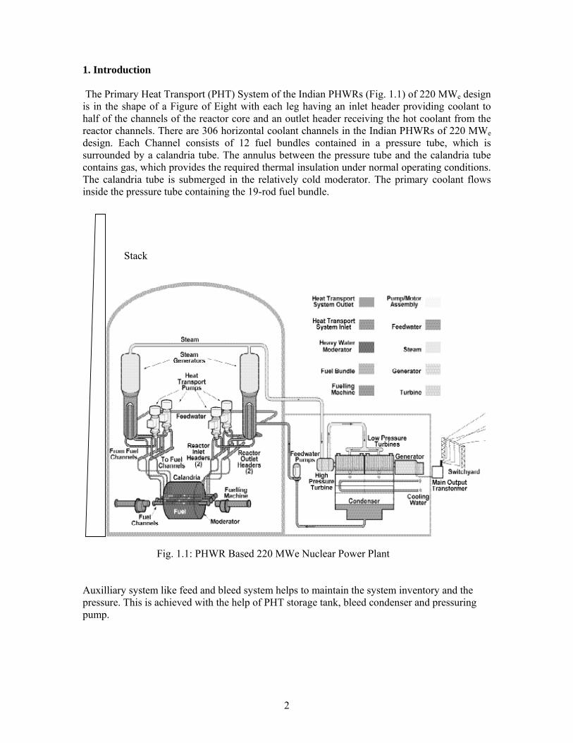
1. Introduction The Primary Heat Transport (PHT) System of the Indian PHWRs (Fig. 1.1) of 220 MWe design is in the shape of a Figure of Eight with each leg having an inlet header providing coolant to half of the channels of the reactor core and an outlet header receiving the hot coolant from the reactor channels. There are 306 horizontal coolant channels in the Indian PHWRs of 220 MWe design. Each Channel consists of 12 fuel bundles contained in a pressure tube, which is surrounded by a calandria tube. The annulus between the pressure tube and the calandria tube contains gas, which provides the required thermal insulation under normal operating conditions. The calandria tube is submerged in the relatively cold moderator. The primary coolant flows inside the pressure tube containing the 19-rod fuel bundle.

Fig. 1.1: PHWR Based 220 MWe Nuclear Power Plant Auxilliary system like feed and bleed system helps to maintain the system inventory and the pressure. This is achieved with the help of PHT storage tank, bleed condenser and pressuring pump.

Stack

3

The reactor is equipped with Emergency Core Cooling System (ECCS) with heavy water and light water hydro accumulators along with long term pumped recirculation system. This system is designed to limit the consequences of event like Loss of Coolant Accident (LOCA).

The PHWR uses a double containment envelope viz, a primary and a secondary containment along with a number of Engineering Safety Features. The primary containment is completely surrounded by the secondary containment.

The primary containment is constructed of prestressed concrete and the secondary containment is of reinforced concrete. Both buildings are cylindrical structures topped by domes. The annular space between the primary and seondary containment envelops is provided with a purging arrangement to maintain negative pressure.The primary containment is divided into two volumes called V1 (drywell) and V2 (wetwell) for efficient accident management. These two volumes are interconnected by a vent system via the suppression pool. The volume V1 houses all the high enthalpy systems like the reactor core, fuelling machine vaults, pump room vaults etc to name a few and is inaccessible during normal operation due to high radiation fields. The volume V2 contains low enthalpy systems like suppression pool and is generally accessible during operation. These two volumes are sealed from each other under normal conditions by the vent pipes submerged in suppresion pool. In the context of design requirements from radioactivity release point of view, the accident scenario considered is a LOCA involving a double ended guillotine rupture of the reactor inlet header. The resulting flashing of high enthalpy liquid into the volume V1 will lead to its pressurization. The pressure differential between volumes V1 and V2 causes the water column in the vents to receed (vent clearing). Once the vents are cleared, it establishes the steam-air mixture flow from V1 to V2. The steam-air mixture bubbles through the pool, where the steam gets condensed completely and the hot air is cooled before passing to volume V2. The suppression pool performs the important function of energy as well as radionuclide managenment. As an energy management feature it limits the peak pressure and temperature in the containment following a LOCA by completely condensing the incomming steam. By limiting the peak pressure, the driving force for leakage of fission products to environment is reduced. Radionuclide management which is a secondary function, involves effective fission product removal by dissolving, trapping, entraining or scrubbing away part of the fission products that reach the pool.

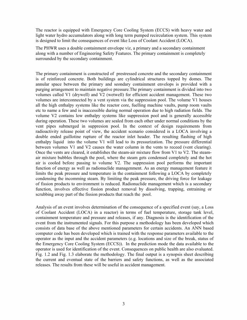
Analysis of an event involves determination of the consequence of a specified event (say, a Loss of Coolant Accident (LOCA) in a reactor) in terms of fuel temperature, storage tank level, containment temperature and pressure and releases, if any. Diagnosis is the identification of the event from the instrumented signals. For this purpose a methodology has been developed which consists of data base of the above mentioned parameters for certain accidents. An ANN based computer code has been developed which is trained with the response parameters available to the operator as the input and the accident parameters (e.g. locations and size of the break, status of the Emergency Core Cooling System (ECCS)). In the prediction mode the data available to the operator is used for identification of the event. Consequences on public health are also evaluated. Fig. 1.2 and Fig. 1.3 elaborate the methodology. The final output is a synopsis sheet describing the current and eventual state of the barriers and safety functions, as well as the associated releases. The results from these will be useful in accident management.

4

Fig. 1.2: Methodology for Identification of Accident Conditions

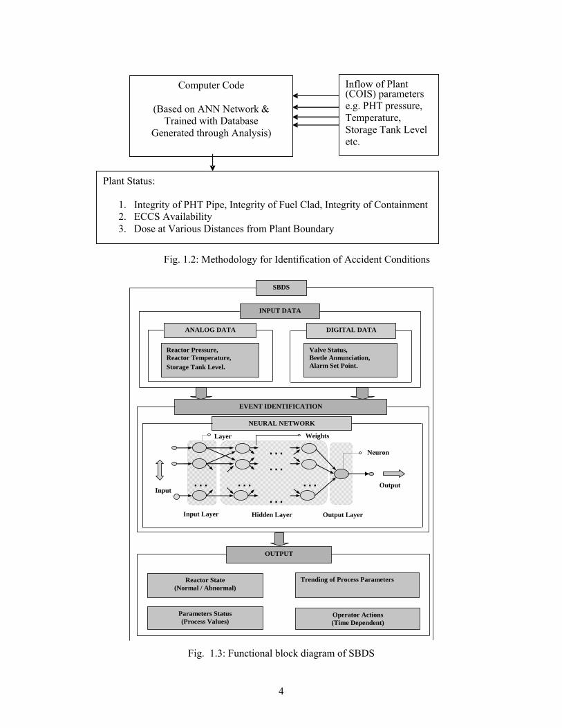
Fig. 1.3: Functional block diagram of SBDS

Computer Code

(Based on ANN Network & Trained with Database

Generated through Analysis)

Inflow of Plant (COIS) parameters e.g. PHT pressure, Temperature, Storage Tank Level etc.

Plant Status:

1. Integrity of PHT Pipe, Integrity of Fuel Clad, Integrity of Containment 2. ECCS Availability 3. Dose at Various Distances from Plant Boundary

SBDS

INPUT DATA

ANALOG DATA DIGITAL DATA

Reactor Pressure, Reactor Temperature, Storage Tank Level.

Valve Status, Beetle Annunciation, Alarm Set Point.

EVENT IDENTIFICATION

NEURAL NETWORK

OUTPUT

Reactor State (Normal / Abnormal)

Operator Actions (Time Dependent)

Trending of Process Parameters

… … ………

…

Weights Layer

Input

Neuron

Parameters Status (Process Values)

Input Layer Output Layer Hidden Layer

Output

5

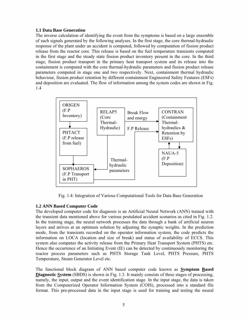
1.1 Data Base Generation The inverse calculation of identifying the event from the symptoms is based on a large ensemble of such signals generated by the following analyses. In the first stage, the core thermal-hydraulic response of the plant under an accident is computed, followed by computation of fission product release from the reactor core. This release is based on the fuel temperature transients computed in the first stage and the steady state fission product inventory present in the core. In the third stage, fission product transport in the primary heat transport system and its release into the containment is computed with the core thermal-hydraulic parameters and fission product release parameters computed in stage one and two respectively. Next, containment thermal hydraulic behaviour, fission product retention by different containment Engineered Safety Features (ESFs) and deposition are evaluated. The flow of information among the system codes are shown in Fig. 1.4 Fig. 1.4: Integration of Various Computational Tools for Data Base Generation 1.2 ANN Based Computer Code The developed computer code for diagnosis is an Artificial Neural Network (ANN) trained with the transient data mentioned above for various postulated accident scenarios as cited in Fig. 1.2. In the training stage, the neural network processes the data through a bank of artificial neuron layers and arrives at an optimum solution by adjusting the synaptic weights. In the prediction mode, from the transients recorded on the operator information system, the code predicts the information on LOCA (location and size of break) and status of availability of ECCS. This system also computes the activity release from the Primary Heat Transport System (PHTS) etc. Hence the occurrence of an Initiating Event (IE) can be detected by continuously monitoring the reactor process parameters such as PHTS Storage Tank Level, PHTS Pressure, PHTS Temperature, Steam Generator Level etc. The functional block diagram of ANN based computer code known as Symptom Based Diagnostic System (SBDS) is shown in Fig. 1.3. It mainly consists of three stages of processing, namely, the input, output and the event identification stage. In the input stage, the data is taken from the Computerized Operator Information System (COIS), processed into a standard file format. This pre-processed data in the input stage is used for training and testing the neural

Thermal-hydraulic parameters

Break Flow and energy F.P Release

ORIGEN (F.P Inventory)

PHTACT (F.P release from fuel)

RELAP5 (Core Thermal-Hydraulic)

CONTRAN (Containment Thermal-hydraulics & Retention by ESFs)

NAUA-5 (F.P Deposition)

SOPHAEROS (F.P Transport in PHT)

6

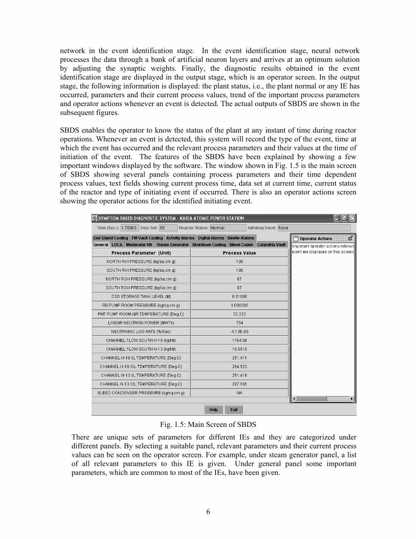
network in the event identification stage. In the event identification stage, neural network processes the data through a bank of artificial neuron layers and arrives at an optimum solution by adjusting the synaptic weights. Finally, the diagnostic results obtained in the event identification stage are displayed in the output stage, which is an operator screen. In the output stage, the following information is displayed: the plant status, i.e., the plant normal or any IE has occurred, parameters and their current process values, trend of the important process parameters and operator actions whenever an event is detected. The actual outputs of SBDS are shown in the subsequent figures. SBDS enables the operator to know the status of the plant at any instant of time during reactor operations. Whenever an event is detected, this system will record the type of the event, time at which the event has occurred and the relevant process parameters and their values at the time of initiation of the event. The features of the SBDS have been explained by showing a few important windows displayed by the software. The window shown in Fig. 1.5 is the main screen of SBDS showing several panels containing process parameters and their time dependent process values, text fields showing current process time, data set at current time, current status of the reactor and type of initiating event if occurred. There is also an operator actions screen showing the operator actions for the identified initiating event.

Fig. 1.5: Main Screen of SBDS

There are unique sets of parameters for different IEs and they are categorized under different panels. By selecting a suitable panel, relevant parameters and their current process values can be seen on the operator screen. For example, under steam generator panel, a list of all relevant parameters to this IE is given. Under general panel some important parameters, which are common to most of the IEs, have been given.

7

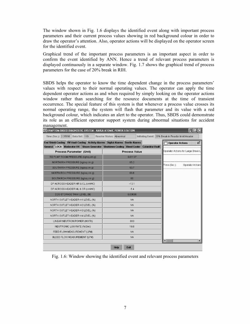
The window shown in Fig. 1.6 displays the identified event along with important process parameters and their current process values showing in red background colour in order to draw the operator’s attention. Also, operator actions will be displayed on the operator screen for the identified event.

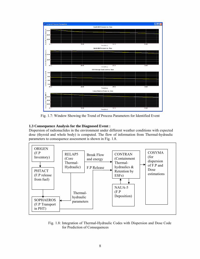
Graphical trend of the important process parameters is an important aspect in order to confirm the event identified by ANN. Hence a trend of relevant process parameters is displayed continuously in a separate window. Fig. 1.7 shows the graphical trend of process parameters for the case of 20% break in RIH.

SBDS helps the operator to know the time dependent change in the process parameters’ values with respect to their normal operating values. The operator can apply the time dependent operator actions as and when required by simply looking on the operator actions window rather than searching for the resource documents at the time of transient occurrence. The special feature of this system is that whenever a process value crosses its normal operating range, the system will flash that parameter and its value with a red background colour, which indicates an alert to the operator. Thus, SBDS could demonstrate its role as an efficient operator support system during abnormal situations for accident management.

Fig. 1.6: Window showing the identified event and relevant process parameters

8

Fig. 1.7: Window Showing the Trend of Process Parameters for Identified Event

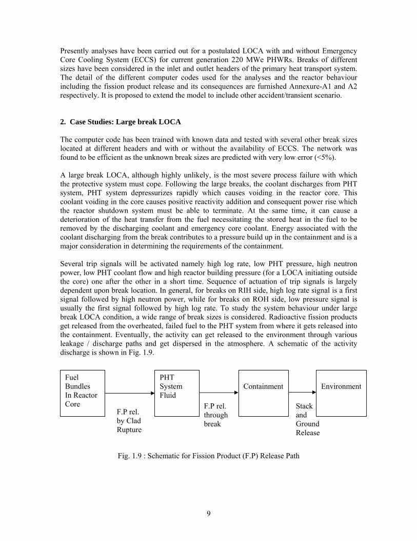
1.3 Consequence Analysis for the Diagnosed Event : Dispersion of radionuclides in the environment under different weather conditions with expected dose (thyroid and whole body) is computed. The flow of information from Thermal-hydraulic parameters to consequence assessment is shown in Fig. 1.8.

Fig. 1.8: Integration of Thermal-Hydraulic Codes with Dispersion and Dose Code

for Prediction of Consequences

Thermal-hydraulic parameters

Break Flow and energy F.P Release

ORIGEN (F.P Inventory)

PHTACT (F.P release from fuel)

RELAP5 (Core Thermal-Hydraulic)

CONTRAN (Containment Thermal-hydraulics & Retention by ESFs)

NAUA-5 (F.P Deposition)

SOPHAEROS (F.P Transport in PHT)

COSYMA (for dispersion of F.P and Dose estimations

9

Presently analyses have been carried out for a postulated LOCA with and without Emergency Core Cooling System (ECCS) for current generation 220 MWe PHWRs. Breaks of different sizes have been considered in the inlet and outlet headers of the primary heat transport system. The detail of the different computer codes used for the analyses and the reactor behaviour including the fission product release and its consequences are furnished Annexure-A1 and A2 respectively. It is proposed to extend the model to include other accident/transient scenario. 2. Case Studies: Large break LOCA The computer code has been trained with known data and tested with several other break sizes located at different headers and with or without the availability of ECCS. The network was found to be efficient as the unknown break sizes are predicted with very low error (<5%). A large break LOCA, although highly unlikely, is the most severe process failure with which the protective system must cope. Following the large breaks, the coolant discharges from PHT system, PHT system depressurizes rapidly which causes voiding in the reactor core. This coolant voiding in the core causes positive reactivity addition and consequent power rise which the reactor shutdown system must be able to terminate. At the same time, it can cause a deterioration of the heat transfer from the fuel necessitating the stored heat in the fuel to be removed by the discharging coolant and emergency core coolant. Energy associated with the coolant discharging from the break contributes to a pressure build up in the containment and is a major consideration in determining the requirements of the containment. Several trip signals will be activated namely high log rate, low PHT pressure, high neutron power, low PHT coolant flow and high reactor building pressure (for a LOCA initiating outside the core) one after the other in a short time. Sequence of actuation of trip signals is largely dependent upon break location. In general, for breaks on RIH side, high log rate signal is a first signal followed by high neutron power, while for breaks on ROH side, low pressure signal is usually the first signal followed by high log rate. To study the system behaviour under large break LOCA condition, a wide range of break sizes is considered. Radioactive fission products get released from the overheated, failed fuel to the PHT system from where it gets released into the containment. Eventually, the activity can get released to the environment through various leakage / discharge paths and get dispersed in the atmosphere. A schematic of the activity discharge is shown in Fig. 1.9.

Fig. 1.9 : Schematic for Fission Product (F.P) Release Path

Fuel Bundles In Reactor Core

F.P rel. by Clad Rupture

Containment

F.P rel. through break

Stack and Ground Release

Environment

PHT System Fluid

10

2.1 Identification of transients using artificial neural networks

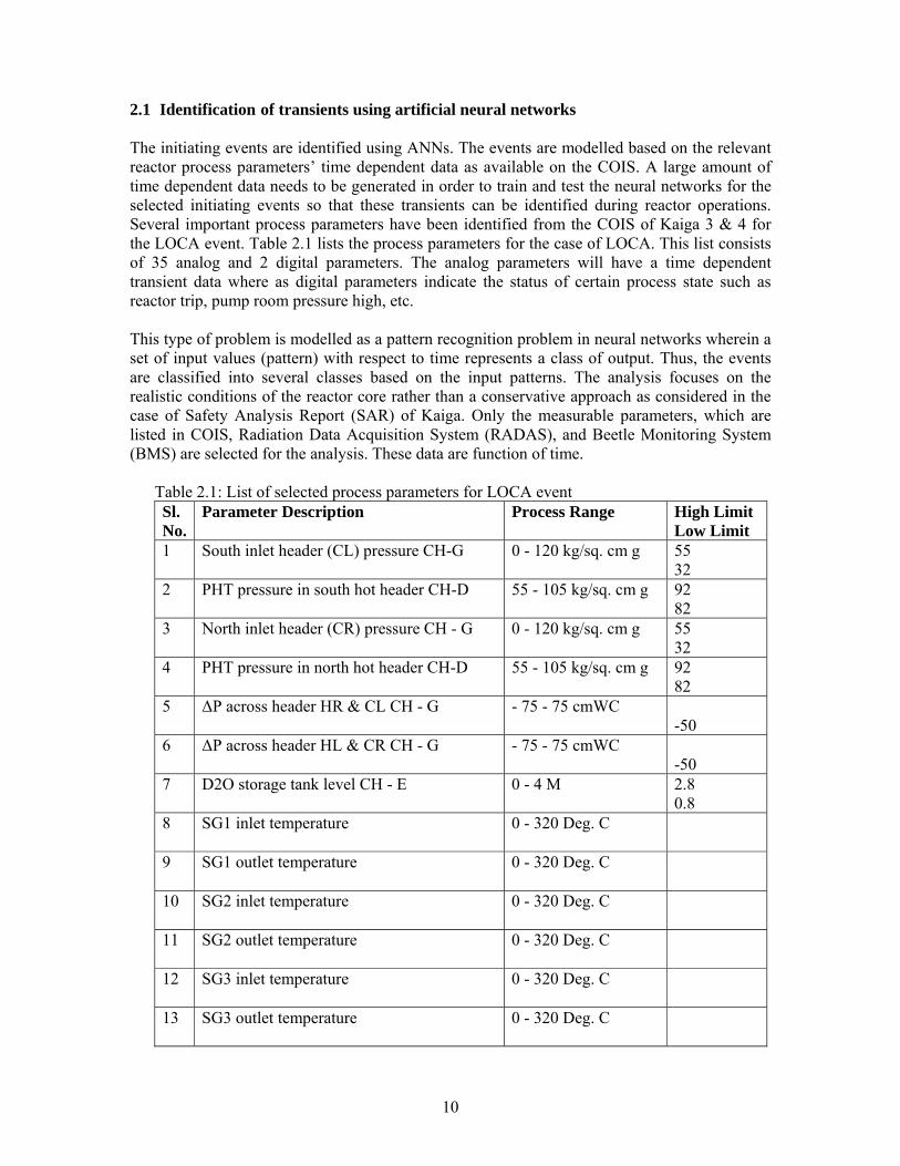
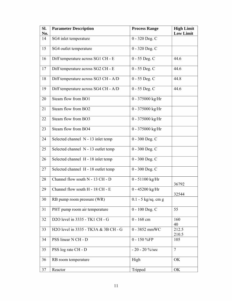
The initiating events are identified using ANNs. The events are modelled based on the relevant reactor process parameters’ time dependent data as available on the COIS. A large amount of time dependent data needs to be generated in order to train and test the neural networks for the selected initiating events so that these transients can be identified during reactor operations. Several important process parameters have been identified from the COIS of Kaiga 3 & 4 for the LOCA event. Table 2.1 lists the process parameters for the case of LOCA. This list consists of 35 analog and 2 digital parameters. The analog parameters will have a time dependent transient data where as digital parameters indicate the status of certain process state such as reactor trip, pump room pressure high, etc.

This type of problem is modelled as a pattern recognition problem in neural networks wherein a set of input values (pattern) with respect to time represents a class of output. Thus, the events are classified into several classes based on the input patterns. The analysis focuses on the realistic conditions of the reactor core rather than a conservative approach as considered in the case of Safety Analysis Report (SAR) of Kaiga. Only the measurable parameters, which are listed in COIS, Radiation Data Acquisition System (RADAS), and Beetle Monitoring System (BMS) are selected for the analysis. These data are function of time.

Table 2.1: List of selected process parameters for LOCA event Sl. No.

Parameter Description Process Range High Limit Low Limit

1 South inlet header (CL) pressure CH-G 0 - 120 kg/sq. cm g 55 32

2 PHT pressure in south hot header CH-D 55 - 105 kg/sq. cm g 92 82

3 North inlet header (CR) pressure CH - G 0 - 120 kg/sq. cm g 55 32

4 PHT pressure in north hot header CH-D 55 - 105 kg/sq. cm g 92 82

5 ΔP across header HR & CL CH - G - 75 - 75 cmWC -50

6 ΔP across header HL & CR CH - G - 75 - 75 cmWC -50

7 D2O storage tank level CH - E 0 - 4 M 2.8 0.8

8 SG1 inlet temperature

0 - 320 Deg. C

9 SG1 outlet temperature

0 - 320 Deg. C


0 - 320 Deg. C


0 - 320 Deg. C


0 - 320 Deg. C


0 - 320 Deg. C

11

Sl. No.

Parameter Description Process Range High Limit Low Limit


0 - 320 Deg. C


0 - 320 Deg. C

16 Diff temperature across SG1 CH - E 0 - 55 Deg. C 44.6

17 Diff temperature across SG2 CH - E 0 - 55 Deg. C 44.6

18 Diff temperature across SG3 CH - A/D

0 - 55 Deg. C 44.8

19 Diff temperature across SG4 CH - A/D 0 - 55 Deg. C 44.6

20 Steam flow from BO1

0 - 375000 kg/Hr


0 - 375000 kg/Hr


0 - 375000 kg/Hr


0 - 375000 kg/Hr

24 Selected channel N - 13 inlet temp

0 - 300 Deg. C

25 Selected channel N - 13 outlet temp

0 - 300 Deg. C

26 Selected channel H - 18 inlet temp

0 - 300 Deg. C

27 Selected channel H - 18 outlet temp

0 - 300 Deg. C

28 Channel flow south N - 13 CH - D

0 - 51100 kg/Hr 36792

29 Channel flow south H - 18 CH - E

0 - 45200 kg/Hr 32544

30 RB pump room pressure (WR) 0.1 - 5 kg/sq. cm g

31 PHT pump room air temperature 0 - 100 Deg. C 55

32 D2O level in 3335 - TK1 CH - G 0 - 168 cm 160 40

33 H2O level in 3335 - TK3A & 3B CH - G 0 - 3852 mmWC 212.5 210.5

34 PSS linear N CH - D 0 - 150 %FP 105

35 PSS log rate CH - D - 20 - 20 %/sec 7

36 RB room temperature High OK

37 Reactor Tripped OK

12

In the first phase of this study, LOCA with and without ECCS events have been considered. The transient data for this case is being generated as described earlier. This transient data base is used to train and test the neural networks for future transient prediction. The breaks considered under Large Break (LB) LOCA are ranging from 20% to 200% break in reactor headers. Small break LOCA with break sizes ranging from 1% to 20% will be analysed. Initially the attempt has been to predict the break size only breaks at specified locations and for a known status of the ECCS. These are described in the Sections 2.1.1 to 2.1.5. Subsequently an ANN has been developed to identify the location and size of the break with the status of the ECCS in a single network. This is described in Section 2.2. 2.1.1 Preliminary ANN study on large break LOCA in RIH with ECCS In order to choose a better network architecture and efficient training scheme, a preliminary study on ANN is conducted. The training and testing of ANN is carried out on different ANN architectures and two training schemes. The break sizes considered for this study are 20%, 60%, 75%, 100%, 120%, 160% and 200% in RIH with ECCS. In addition to these break cases, normal operating condition of the reactor is simulated. A 60 seconds transient duration is chosen in this case under the assumption that this time duration is sufficient to identify the large break LOCA event.

2.1.1.1 Transient data generation In order for training the neural networks, a continuous and consistent data is needed. For this purpose, the time scale of the transient duration is divided into different intervals such that the transient can be identified as quickly as possible in the earlier phase of its development. At the same time, the time scale is chosen such that the number of data points at later period of transient is limited to avoid a long training of ANN. The time scale for a transient period of 60 seconds is as follows:

Δt = 0.01 for t = 0 to 2 secs Δt = 0.1 for t = 2.1 to 30 secs Δt = 0.5 for t = 30.5 to 60 secs

where t is the transient time and Δt is the time increment. The data for analog parameters listed in Table 4.1 with the above time scale is generated from the RELAP 5 thermal-hydraulic code for the transient duration of 60 seconds.

2.1.1.2 Training and Testing Data Preparation The data for training and testing of ANN is selected such that it is uniformly distributed over the transient period. A few break sizes are selected for prediction such that the training and testing data is adequate and consistent with the prediction data. Here, two types of ANN generalization schemes are considered in order to find a best suitable generalization scheme.

All IEs: For the case of all IEs, the alternate data sets of each of the break size data is taken as the training / testing data for that break size. Such data sets of different break sizes are combined into a single file to form the final training / testing file for ANN. In other words,

13

training and testing files should not contain the common data set of the same break size. The training and testing files referred in this case as AllIEsTrg and AllIEsTst respectively. Selected IEs: For the case of selected IEs, the entire data of each break size is taken as the training / testing data for that break size. All the individual break size data considered for training / testing are combined into a single file to form the final training / testing file. In other words, the training and testing data files should not contain the same break size data. The training and testing files referred in this case as SelIEsTrg and SelIEsTst respectively. Table 2.2 illustrates the two above mentioned schemes for training / testing of ANN. The break size 0% corresponds to the normal reactor operating condition.

Table 2.2: Training/testing schemes for ANN Selected IEs

(Entire data of selected break is used for training/testing)

All IEs (Alternate pattern of all breaks is

used for training/testing)

Training (SelIEsTrg)

Testing / Prediction (SelIEsTst)

Training (AllIEsTrg)

Testing (AllIEsTst)

0% 75% 0% 0% 20% 120% 20% 20% 60% 200% 60% 60% 100% 75% 75% 160% 100% 100% 120% 120% 160% 160% 200% 200%

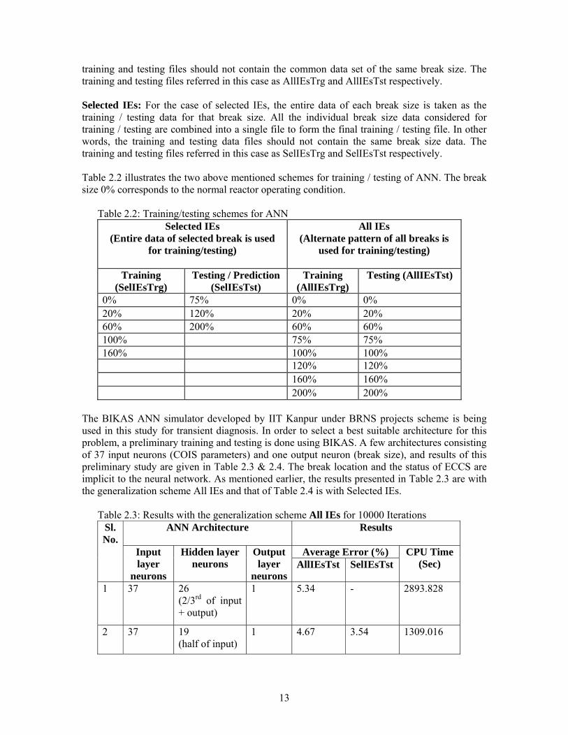
The BIKAS ANN simulator developed by IIT Kanpur under BRNS projects scheme is being used in this study for transient diagnosis. In order to select a best suitable architecture for this problem, a preliminary training and testing is done using BIKAS. A few architectures consisting of 37 input neurons (COIS parameters) and one output neuron (break size), and results of this preliminary study are given in Table 2.3 & 2.4. The break location and the status of ECCS are implicit to the neural network. As mentioned earlier, the results presented in Table 2.3 are with the generalization scheme All IEs and that of Table 2.4 is with Selected IEs.

Table 2.3: Results with the generalization scheme All IEs for 10000 Iterations Sl. No.

ANN Architecture Results

Input layer

neurons

Hidden layer neurons

Output layer

neurons

Average Error (%) CPU Time (Sec)

AllIEsTst SelIEsTst

1 37 26 (2/3rd of input + output)

1 5.34 - 2893.828

2 37 19 (half of input)

1 4.67 3.54 1309.016

14

3 37 26 19 1 37.22 44.75 8919.157 (Iterations: 3580)

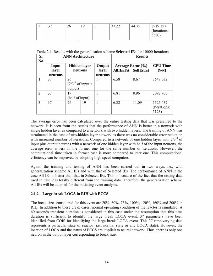
Table 2.4: Results with the generalization scheme Selected IEs for 10000 Iterations Sl. No.

ANN Architecture Results

Input layer

neurons

Hidden layer neurons

Output layer

neurons

Average Error (%) CPU Time (Sec)

AllIEsTst SelIEsTst

1 37 26 (2/3rd of input + output)

1 6.58 8.67 3648.032

2 37 19 (half of input)

1 6.81 8.96 3097.906

3 37 26 19 1 6.82 11.09 5526.437 (Iterations: 5123)

The average error has been calculated over the entire testing data that was presented to the network. It is seen from the results that the performance of ANN is better in a network with single hidden layer as compared to a network with two hidden layers. The training of ANN was terminated in the case of two-hidden layer network as there was no considerable error reduction with increased number of iterations. Compared to a network of one hidden layer with 2/3rd of input plus output neurons with a network of one hidden layer with half of the input neurons, the average error is less in the former one for the same number of iterations. However, the computational time taken in former case is more compared to later one. This computational efficiency can be improved by adopting high speed computers.

Again, the training and testing of ANN has been carried out in two ways, i.e., with generalization scheme All IEs and with that of Selected IEs. The performance of ANN in the case All IEs is better than that in Selected IEs. This is because of the fact that the testing data used in case 2 is totally different from the training data. Therefore, the generalization scheme All IEs will be adopted for the initiating event analysis.

2.1.2 Large break LOCA in RIH with ECCS The break sizes considered for this event are 20%, 60%, 75%, 100%, 120%, 160% and 200% in RIH. In addition to these break cases, normal operating condition of the reactor is simulated. A 60 seconds transient duration is considered in this case under the assumption that this time duration is sufficient to identify the large break LOCA event. 37 parameters have been identified from COIS for identifying the large break LOCA event. This 37 time-varying data represents a particular state of reactor (i.e., normal state or any LOCA state). However, the location of LOCA and the status of ECCS are implicit to neural network. Thus, there is only one neuron in the output layer corresponding to break size.

15

2.1.2.1 Network parameters for ANN training for large break LOCA in RIH with ECCS

Network Architecture

Input Neurons : Hidden Neurons: Output Neurons

37 × 26 × 1

Training Algorithm: First Order Resilient Back Propagation Activation Function: Unipolar Sigmoid Error Function: Sum Squared Error Learning Rate: 0.7 Weights: ±0.5 Target Error:1.0E-6

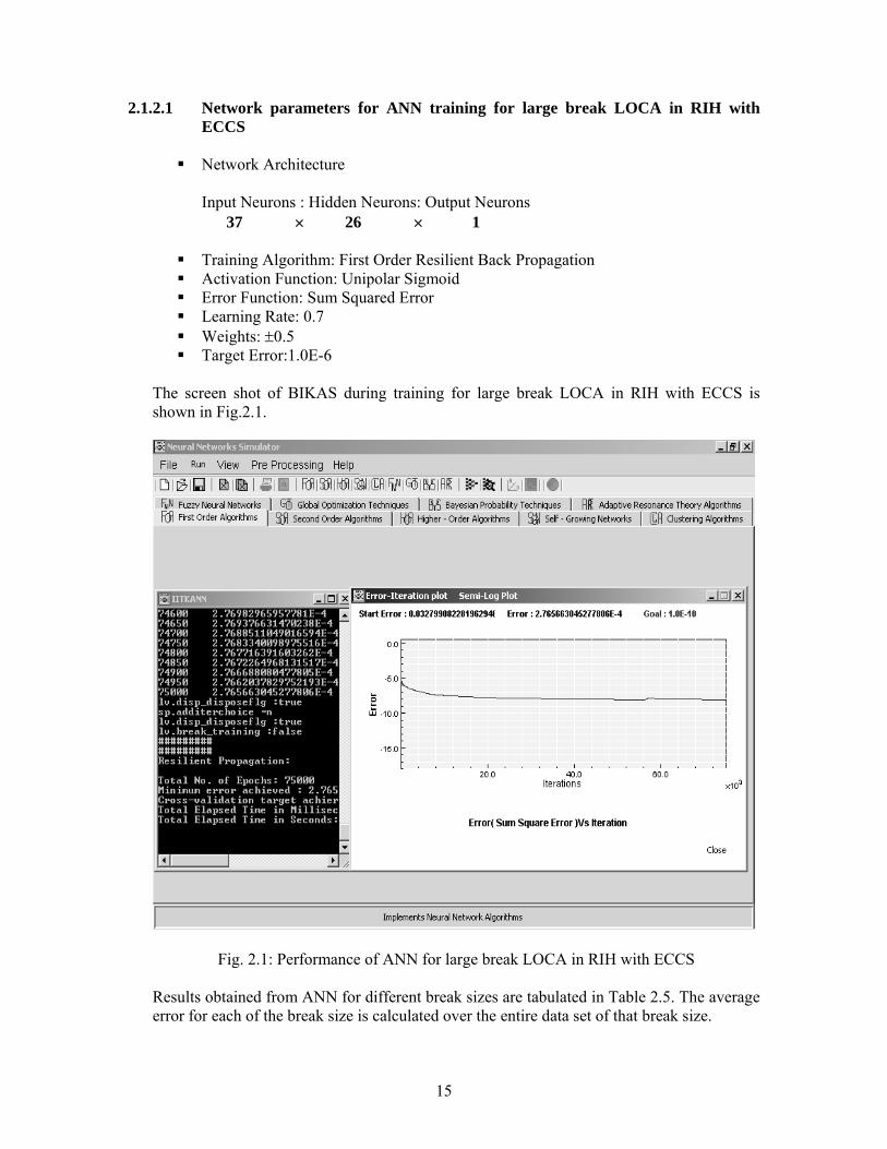
The screen shot of BIKAS during training for large break LOCA in RIH with ECCS is shown in Fig.2.1.

Fig. 2.1: Performance of ANN for large break LOCA in RIH with ECCS

Results obtained from ANN for different break sizes are tabulated in Table 2.5. The average error for each of the break size is calculated over the entire data set of that break size.

16

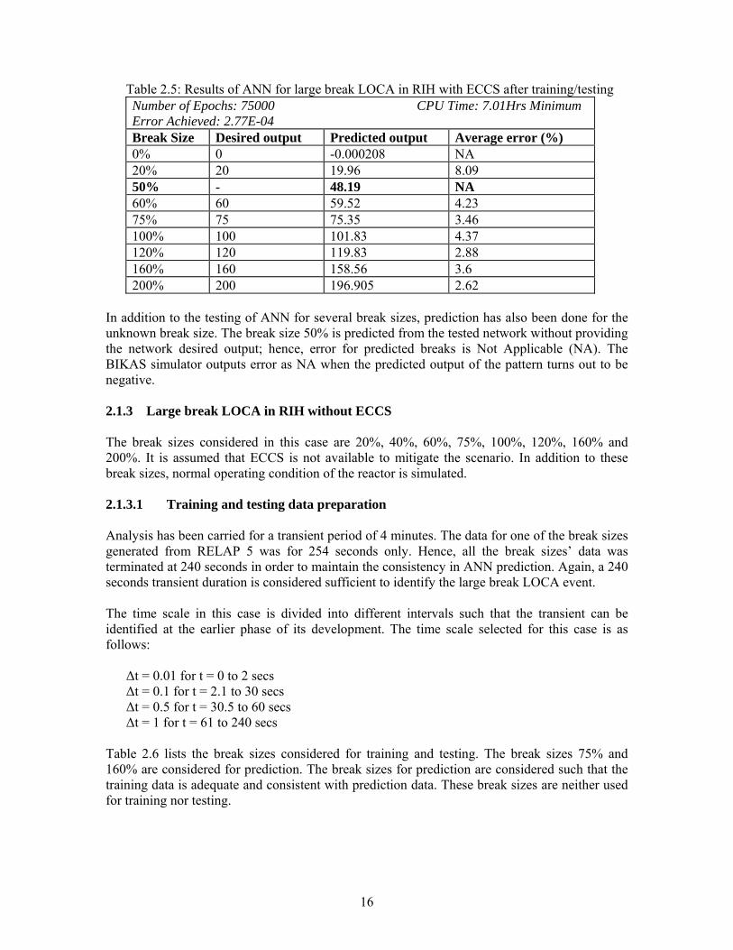
Table 2.5: Results of ANN for large break LOCA in RIH with ECCS after training/testing Number of Epochs: 75000 CPU Time: 7.01Hrs Minimum Error Achieved: 2.77E-04 Break Size Desired output Predicted output Average error (%) 0% 0 -0.000208 NA 20% 20 19.96 8.09 50% - 48.19 NA 60% 60 59.52 4.23 75% 75 75.35 3.46 100% 100 101.83 4.37 120% 120 119.83 2.88 160% 160 158.56 3.6 200% 200 196.905 2.62

In addition to the testing of ANN for several break sizes, prediction has also been done for the unknown break size. The break size 50% is predicted from the tested network without providing the network desired output; hence, error for predicted breaks is Not Applicable (NA). The BIKAS simulator outputs error as NA when the predicted output of the pattern turns out to be negative. 2.1.3 Large break LOCA in RIH without ECCS The break sizes considered in this case are 20%, 40%, 60%, 75%, 100%, 120%, 160% and 200%. It is assumed that ECCS is not available to mitigate the scenario. In addition to these break sizes, normal operating condition of the reactor is simulated. 2.1.3.1 Training and testing data preparation Analysis has been carried for a transient period of 4 minutes. The data for one of the break sizes generated from RELAP 5 was for 254 seconds only. Hence, all the break sizes’ data was terminated at 240 seconds in order to maintain the consistency in ANN prediction. Again, a 240 seconds transient duration is considered sufficient to identify the large break LOCA event.

The time scale in this case is divided into different intervals such that the transient can be identified at the earlier phase of its development. The time scale selected for this case is as follows:

Δt = 0.01 for t = 0 to 2 secs Δt = 0.1 for t = 2.1 to 30 secs Δt = 0.5 for t = 30.5 to 60 secs Δt = 1 for t = 61 to 240 secs

Table 2.6 lists the break sizes considered for training and testing. The break sizes 75% and 160% are considered for prediction. The break sizes for prediction are considered such that the training data is adequate and consistent with prediction data. These break sizes are neither used for training nor testing.

17

Table 2.6: Break sizes for training and testing of ANN Training Testing Prediction 0% 0% 75% 20% 20% 160% 40% 40% 60% 60% 100% 100% 120% 120% 150% 150% 200% 200%

2.1.3.2 The parameters for ANN for large break LOCA in RIH without ECCS

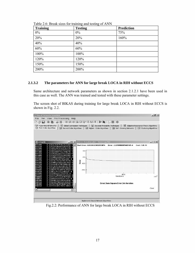
Same architecture and network parameters as shown in section 2.1.2.1 have been used in this case as well. The ANN was trained and tested with these parameter settings. The screen shot of BIKAS during training for large break LOCA in RIH without ECCS is shown in Fig. 2.2.

Fig.2.2: Performance of ANN for large break LOCA in RIH without ECCS

18

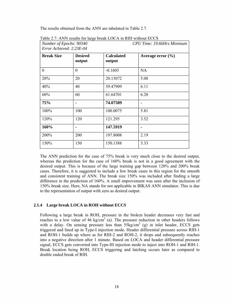
The results obtained from the ANN are tabulated in Table 2.7. Table 2.7: ANN results for large break LOCA in RIH without ECCS Number of Epochs: 90340 CPU Time: 19.66Hrs Minimum Error Achieved: 2.23E-04

Break Size Desired output

Calculated output

Average error (%)

0 0 -0.1603 NA

20% 20 20.13072 5.08

40% 40 39.47909 6.11

60% 60 61.64701 6.20

75% - 74.07589 -

100% 100 100.0075 5.81

120% 120 121.295 3.52

160% - 147.5919 -

200% 200 197.8008 2.19

150% 150 150.1388 3.33

The ANN prediction for the case of 75% break is very much close to the desired output, whereas the prediction for the case of 160% break is not in a good agreement with the desired output. This is because of the large training gap between 120% and 200% break cases. Therefore, it is suggested to include a few break cases in this region for the smooth and consistent training of ANN. The break size 150% was included after finding a large difference in the prediction of 160%. A small improvement was seen after the inclusion of 150% break size. Here, NA stands for not applicable in BIKAS ANN simulator. This is due to the representation of output with zero as desired output.

2.1.4 Large break LOCA in ROH without ECCS Following a large break in ROH, pressure in the broken header decreases very fast and reaches to a low value of 46 kg/cm2 (a). The pressure reduction in other headers follows with a delay. On sensing pressure less than 55kg/cm2 (g) in inlet header, ECCS gets triggered and lined up in Type-I injection mode. Header differential pressure across RIH-1 and ROH-1 builds up where as for RIH-2 and ROH-2, it drops and subsequently reaches into a negative direction after 1 minute. Based on LOCA and header differential pressure signal, ECCS gets converted into Type-III injection mode to inject into ROH-1 and RIH-1. Break location being ROH, ECCS triggering and latching occurs later as compared to double ended break of RIH.

19

The break sizes considered in this case are 20%, 40%, 60%, 75%, 100%, 120%, 160% and 200%. In addition to these break sizes, normal operating condition of the reactor is simulated.

2.1.4.1 Transient data generation

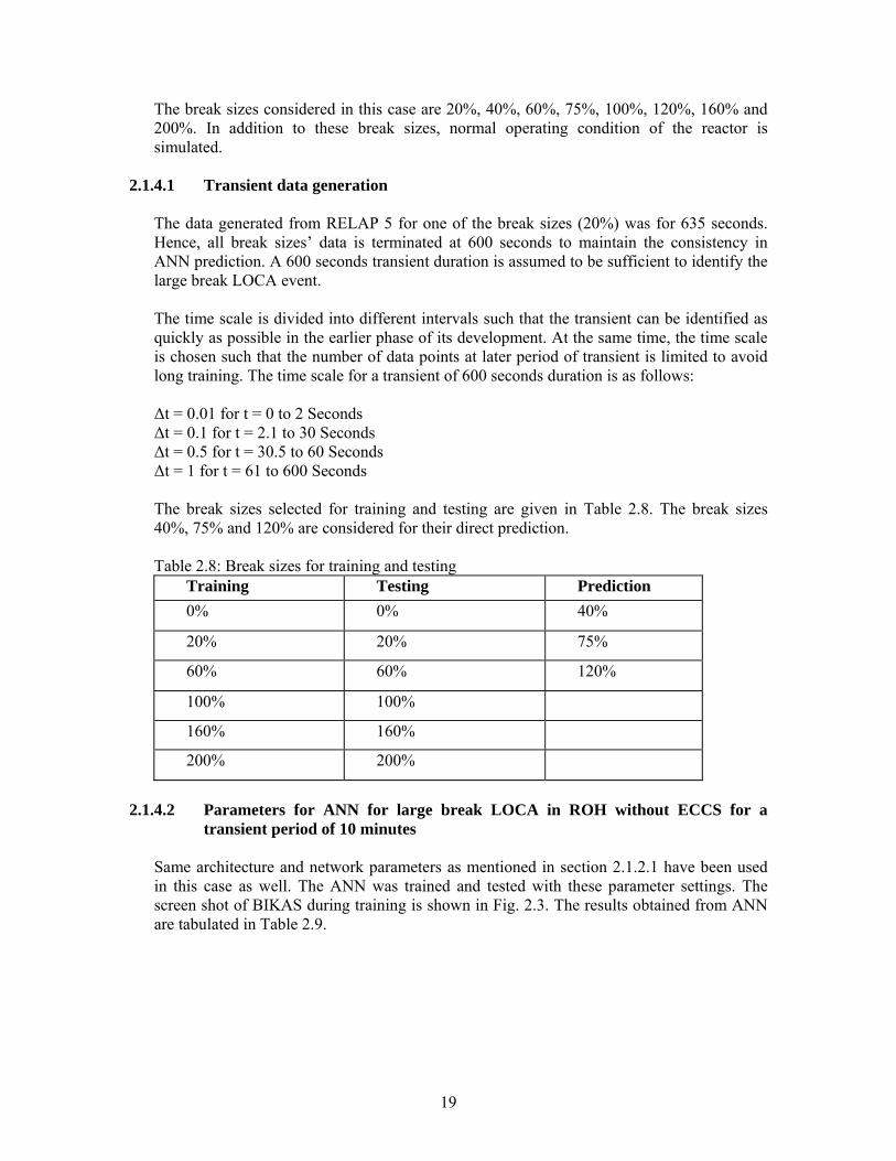
The data generated from RELAP 5 for one of the break sizes (20%) was for 635 seconds. Hence, all break sizes’ data is terminated at 600 seconds to maintain the consistency in ANN prediction. A 600 seconds transient duration is assumed to be sufficient to identify the large break LOCA event. The time scale is divided into different intervals such that the transient can be identified as quickly as possible in the earlier phase of its development. At the same time, the time scale is chosen such that the number of data points at later period of transient is limited to avoid long training. The time scale for a transient of 600 seconds duration is as follows: Δt = 0.01 for t = 0 to 2 Seconds Δt = 0.1 for t = 2.1 to 30 Seconds Δt = 0.5 for t = 30.5 to 60 Seconds Δt = 1 for t = 61 to 600 Seconds The break sizes selected for training and testing are given in Table 2.8. The break sizes 40%, 75% and 120% are considered for their direct prediction. Table 2.8: Break sizes for training and testing

Training Testing Prediction 0% 0% 40%

20% 20% 75%

60% 60% 120%

100% 100%

160% 160%

200% 200%

2.1.4.2 Parameters for ANN for large break LOCA in ROH without ECCS for a

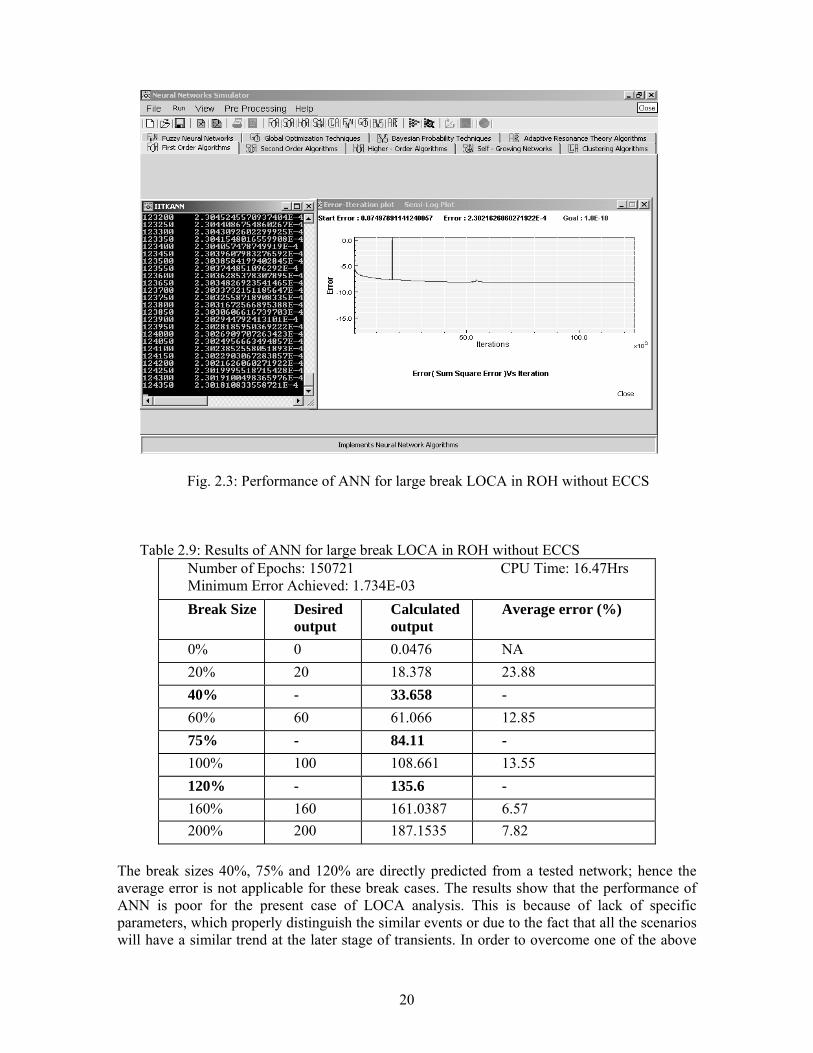
transient period of 10 minutes Same architecture and network parameters as mentioned in section 2.1.2.1 have been used in this case as well. The ANN was trained and tested with these parameter settings. The screen shot of BIKAS during training is shown in Fig. 2.3. The results obtained from ANN are tabulated in Table 2.9.

20

Fig. 2.3: Performance of ANN for large break LOCA in ROH without ECCS Table 2.9: Results of ANN for large break LOCA in ROH without ECCS

Number of Epochs: 150721 CPU Time: 16.47Hrs Minimum Error Achieved: 1.734E-03 Break Size Desired

output Calculated output

Average error (%)

0% 0 0.0476 NA 20% 20 18.378 23.88 40% - 33.658 - 60% 60 61.066 12.85 75% - 84.11 - 100% 100 108.661 13.55 120% - 135.6 - 160% 160 161.0387 6.57 200% 200 187.1535 7.82

The break sizes 40%, 75% and 120% are directly predicted from a tested network; hence the average error is not applicable for these break cases. The results show that the performance of ANN is poor for the present case of LOCA analysis. This is because of lack of specific parameters, which properly distinguish the similar events or due to the fact that all the scenarios will have a similar trend at the later stage of transients. In order to overcome one of the above

21

mentioned aspects, the transient duration is considered for initial 4 minutes for further analysis. This 4 minutes data is used for training and testing of ANN for large break LOCA in ROH without ECCS.

2.1.4.3 Network parameters for ANN for large break LOCA in ROH without ECCS

for a transient period of 4 minutes

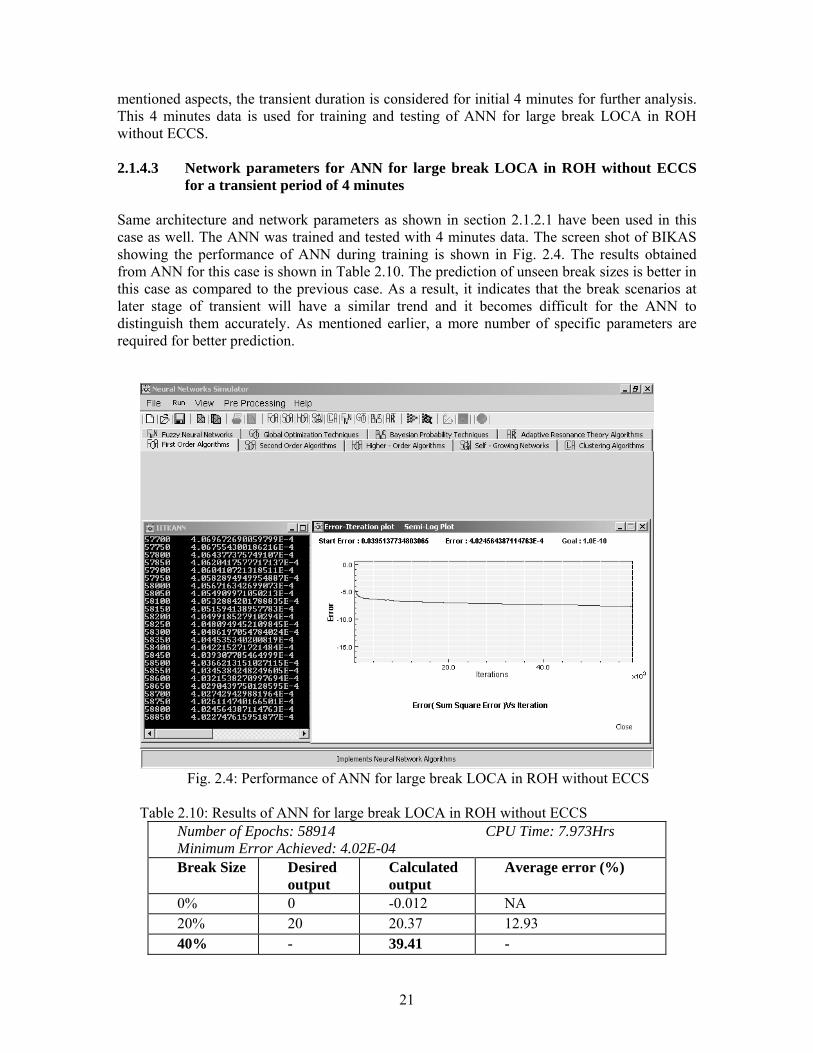
Same architecture and network parameters as shown in section 2.1.2.1 have been used in this case as well. The ANN was trained and tested with 4 minutes data. The screen shot of BIKAS showing the performance of ANN during training is shown in Fig. 2.4. The results obtained from ANN for this case is shown in Table 2.10. The prediction of unseen break sizes is better in this case as compared to the previous case. As a result, it indicates that the break scenarios at later stage of transient will have a similar trend and it becomes difficult for the ANN to distinguish them accurately. As mentioned earlier, a more number of specific parameters are required for better prediction.

Fig. 2.4: Performance of ANN for large break LOCA in ROH without ECCS

Table 2.10: Results of ANN for large break LOCA in ROH without ECCS



Average error (%)

0% 0 -0.012 NA 20% 20 20.37 12.93 40% - 39.41 -

22

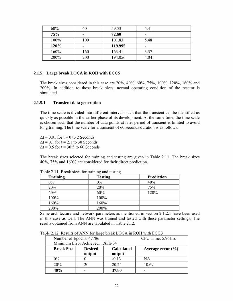
60% 60 59.53 5.41 75% - 72.60 - 100% 100 101.83 5.48 120% - 119.995 - 160% 160 163.41 3.37 200% 200 194.056 4.04

2.1.5 Large break LOCA in ROH with ECCS

The break sizes considered in this case are 20%, 40%, 60%, 75%, 100%, 120%, 160% and 200%. In addition to these break sizes, normal operating condition of the reactor is simulated.

2.1.5.1 Transient data generation

The time scale is divided into different intervals such that the transient can be identified as quickly as possible in the earlier phase of its development. At the same time, the time scale is chosen such that the number of data points at later period of transient is limited to avoid long training. The time scale for a transient of 60 seconds duration is as follows: Δt = 0.01 for t = 0 to 2 Seconds Δt = 0.1 for t = 2.1 to 30 Seconds Δt = 0.5 for t = 30.5 to 60 Seconds The break sizes selected for training and testing are given in Table 2.11. The break sizes 40%, 75% and 160% are considered for their direct prediction. Table 2.11: Break sizes for training and testing

Training Testing Prediction 0% 0% 40% 20% 20% 75% 60% 60% 120% 100% 100% 160% 160% 200% 200%

Same architecture and network parameters as mentioned in section 2.1.2.1 have been used in this case as well. The ANN was trained and tested with these parameter settings. The results obtained from ANN are tabulated in Table 2.12. Table 2.12: Results of ANN for large break LOCA in ROH with ECCS



Average error (%)

0% 0 -0.13 NA 20% 20 20.24 10.69 40% - 37.80 -

23

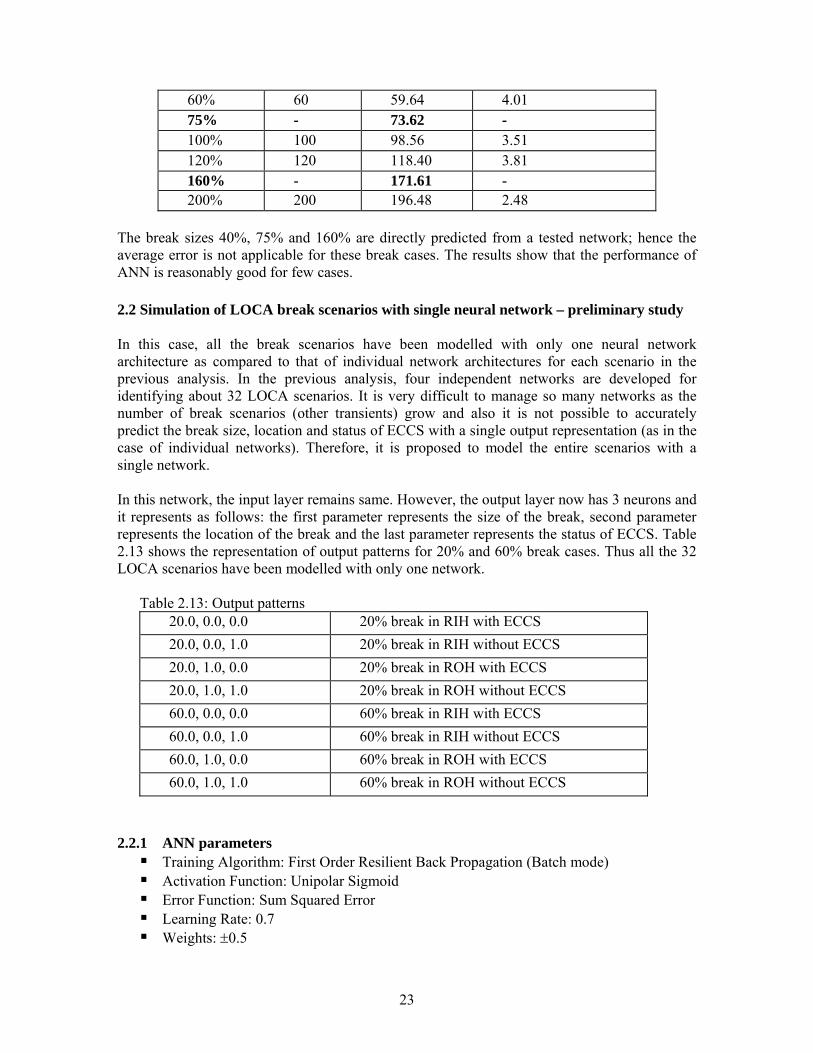
60% 60 59.64 4.01 75% - 73.62 - 100% 100 98.56 3.51 120% 120 118.40 3.81 160% - 171.61 - 200% 200 196.48 2.48

The break sizes 40%, 75% and 160% are directly predicted from a tested network; hence the average error is not applicable for these break cases. The results show that the performance of ANN is reasonably good for few cases. 2.2 Simulation of LOCA break scenarios with single neural network – preliminary study In this case, all the break scenarios have been modelled with only one neural network architecture as compared to that of individual network architectures for each scenario in the previous analysis. In the previous analysis, four independent networks are developed for identifying about 32 LOCA scenarios. It is very difficult to manage so many networks as the number of break scenarios (other transients) grow and also it is not possible to accurately predict the break size, location and status of ECCS with a single output representation (as in the case of individual networks). Therefore, it is proposed to model the entire scenarios with a single network. In this network, the input layer remains same. However, the output layer now has 3 neurons and it represents as follows: the first parameter represents the size of the break, second parameter represents the location of the break and the last parameter represents the status of ECCS. Table 2.13 shows the representation of output patterns for 20% and 60% break cases. Thus all the 32 LOCA scenarios have been modelled with only one network.

Table 2.13: Output patterns 20.0, 0.0, 0.0 20% break in RIH with ECCS 20.0, 0.0, 1.0 20% break in RIH without ECCS 20.0, 1.0, 0.0 20% break in ROH with ECCS 20.0, 1.0, 1.0 20% break in ROH without ECCS 60.0, 0.0, 0.0 60% break in RIH with ECCS 60.0, 0.0, 1.0 60% break in RIH without ECCS 60.0, 1.0, 0.0 60% break in ROH with ECCS 60.0, 1.0, 1.0 60% break in ROH without ECCS

2.2.1 ANN parameters

Training Algorithm: First Order Resilient Back Propagation (Batch mode) Activation Function: Unipolar Sigmoid Error Function: Sum Squared Error Learning Rate: 0.7 Weights: ±0.5

24

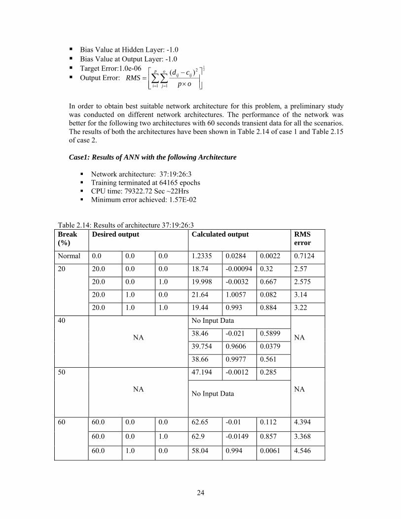
Bias Value at Hidden Layer: -1.0 Bias Value at Output Layer: -1.0 Target Error:1.0e-06 Output Error:

In order to obtain best suitable network architecture for this problem, a preliminary study was conducted on different network architectures. The performance of the network was better for the following two architectures with 60 seconds transient data for all the scenarios. The results of both the architectures have been shown in Table 2.14 of case 1 and Table 2.15 of case 2.

Case1: Results of ANN with the following Architecture

Network architecture: 37:19:26:3 Training terminated at 64165 epochs CPU time: 79322.72 Sec ~22Hrs Minimum error achieved: 1.57E-02

Table 2.14: Results of architecture 37:19:26:3 Break (%)

Desired output Calculated output RMS error

Normal 0.0 0.0 0.0 1.2335 0.0284 0.0022 0.7124

20 20.0 0.0 0.0 18.74 -0.00094 0.32 2.57

20.0 0.0 1.0 19.998 -0.0032 0.667 2.575

20.0 1.0 0.0 21.64 1.0057 0.082 3.14

20.0 1.0 1.0 19.44 0.993 0.884 3.22

40

NA

No Input Data NA 38.46 -0.021 0.5899

39.754 0.9606 0.0379

38.66 0.9977 0.561

50

NA

47.194 -0.0012 0.285 NA

No Input Data

60 60.0 0.0 0.0 62.65 -0.01 0.112 4.394

60.0 0.0 1.0 62.9 -0.0149 0.857 3.368

60.0 1.0 0.0 58.04 0.994 0.0061 4.546

21

1 1

2)(

⎥⎥⎦

⎤

⎢⎢⎣

⎡

×

−= ∑∑

= =

p

i

o

j

ijij

opcd

RMS

25

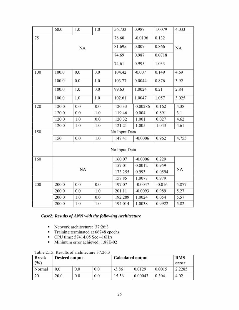
60.0 1.0 1.0 56.733 0.987 1.0079 4.033

75

NA

78.60 -0.0196 0.132 NA 81.695 0.007 0.866

74.69 0.987 0.0718

74.61 0.995 1.033

100 100.0 0.0 0.0 104.42 -0.007 0.149 4.69

100.0 0.0 1.0 103.77 0.0044 0.876 3.92

100.0 1.0 0.0 99.63 1.0024 0.21 2.84

100.0 1.0 1.0 102.61 1.0047 1.057 3.025

120 120.0 0.0 0.0 120.33 0.00286 0.162 4.38 120.0 0.0 1.0 119.46 0.004 0.891 3.1 120.0 1.0 0.0 120.32 1.001 0.027 4.62 120.0 1.0 1.0 121.21 1.005 1.043 4.61

150 No Input Data 150 0.0 1.0 147.41 -0.0006 0.962 4.755

No Input Data

160

NA

160.07 -0.0006 0.229 NA

157.01 0.0012 0.959 173.255 0.993 0.0594 157.85 1.0077 0.979

200 200.0 0.0 0.0 197.07 -0.0047 -0.016 5.877 200.0 0.0 1.0 201.11 -0.0093 0.989 5.27 200.0 1.0 0.0 192.289 1.0024 0.054 5.57 200.0 1.0 1.0 194.014 1.0038 0.9922 5.82

Case2: Results of ANN with the following Architecture

Network architecture: 37:26:3 Training terminated at 66748 epochs CPU time: 57414.05 Sec ~16Hrs Minimum error achieved: 1.88E-02

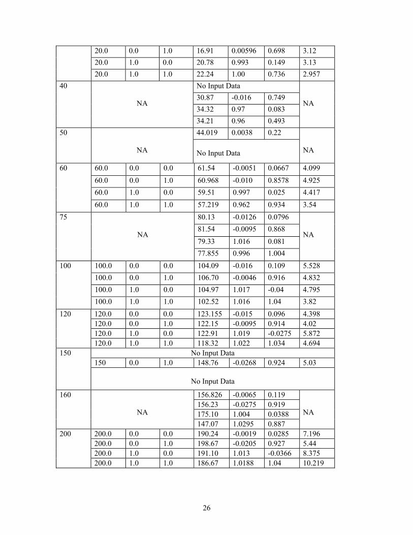
Table 2.15: Results of architecture 37:26:3 Break (%)


Normal 0.0 0.0 0.0 -3.86 0.0129 0.0015 2.2285 20 20.0 0.0 0.0 15.56 0.00043 0.304 4.02

26

20.0 0.0 1.0 16.91 0.00596 0.698 3.12 20.0 1.0 0.0 20.78 0.993 0.149 3.13 20.0 1.0 1.0 22.24 1.00 0.736 2.957

40

NA

No Input Data NA

30.87 -0.016 0.749 34.32 0.97 0.083 34.21 0.96 0.493

50

NA

44.019 0.0038 0.22 NA

No Input Data

60 60.0 0.0 0.0 61.54 -0.0051 0.0667 4.099 60.0 0.0 1.0 60.968 -0.010 0.8578 4.925 60.0 1.0 0.0 59.51 0.997 0.025 4.417 60.0 1.0 1.0 57.219 0.962 0.934 3.54

75

NA

80.13 -0.0126 0.0796 NA

81.54 -0.0095 0.868 79.33 1.016 0.081 77.855 0.996 1.004

100 100.0 0.0 0.0 104.09 -0.016 0.109 5.528 100.0 0.0 1.0 106.70 -0.0046 0.916 4.832 100.0 1.0 0.0 104.97 1.017 -0.04 4.795 100.0 1.0 1.0 102.52 1.016 1.04 3.82

120 120.0 0.0 0.0 123.155 -0.015 0.096 4.398 120.0 0.0 1.0 122.15 -0.0095 0.914 4.02 120.0 1.0 0.0 122.91 1.019 -0.0275 5.872 120.0 1.0 1.0 118.32 1.022 1.034 4.694

150 No Input Data 150 0.0 1.0 148.76 -0.0268 0.924 5.03

No Input Data

160

NA

156.826 -0.0065 0.119 NA

156.23 -0.0275 0.919 175.10 1.004 0.0388 147.07 1.0295 0.887

200 200.0 0.0 0.0 190.24 -0.0019 0.0285 7.196 200.0 0.0 1.0 198.67 -0.0205 0.927 5.44 200.0 1.0 0.0 191.10 1.013 -0.0366 8.375 200.0 1.0 1.0 186.67 1.0188 1.04 10.219

27

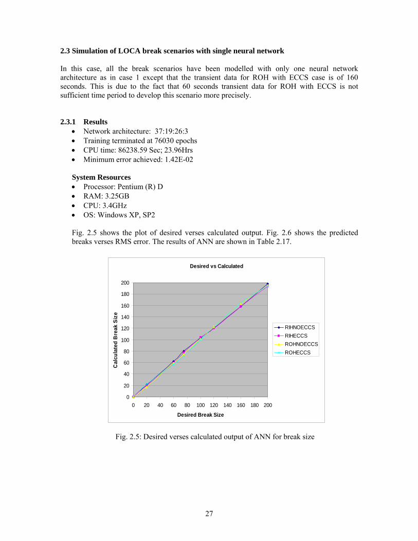
2.3 Simulation of LOCA break scenarios with single neural network In this case, all the break scenarios have been modelled with only one neural network architecture as in case 1 except that the transient data for ROH with ECCS case is of 160 seconds. This is due to the fact that 60 seconds transient data for ROH with ECCS is not sufficient time period to develop this scenario more precisely.

2.3.1 Results • Network architecture: 37:19:26:3 • Training terminated at 76030 epochs • CPU time: 86238.59 Sec; 23.96Hrs • Minimum error achieved: 1.42E-02

System Resources • Processor: Pentium (R) D • RAM: 3.25GB • CPU: 3.4GHz • OS: Windows XP, SP2 Fig. 2.5 shows the plot of desired verses calculated output. Fig. 2.6 shows the predicted breaks verses RMS error. The results of ANN are shown in Table 2.17.

Fig. 2.5: Desired verses calculated output of ANN for break size

Desired vs Calculated

0

20

40

60

80

100

120

140

160

180

200

0 20 40 60 80 100 120 140 160 180 200

Desired Break Size

Cal

cula

ted

Bre

ak S

ize

RIHNOECCSRIHECCSROHNOECCSROHECCS

28

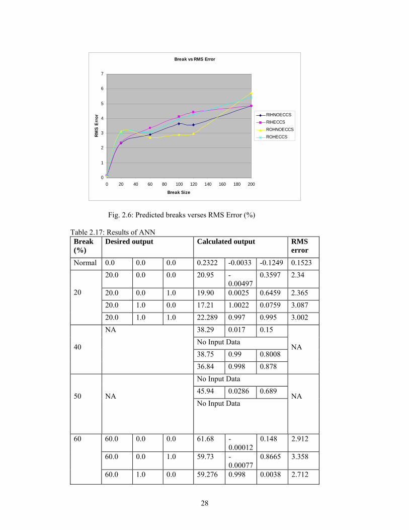
Fig. 2.6: Predicted breaks verses RMS Error (%) Table 2.17: Results of ANN Break (%)


Normal 0.0 0.0 0.0 0.2322 -0.0033 -0.1249 0.1523 20

20.0 0.0 0.0 20.95 -0.00497

0.3597 2.34

20.0 0.0 1.0 19.90 0.0025 0.6459 2.365 20.0 1.0 0.0 17.21 1.0022 0.0759 3.087 20.0 1.0 1.0 22.289 0.997 0.995 3.002

40

NA 38.29 0.017 0.15 NA

No Input Data 38.75 0.99 0.8008 36.84 0.998 0.878

50

NA

No Input Data NA

45.94 0.0286 0.689 No Input Data

60 60.0 0.0 0.0 61.68 -0.00012

0.148 2.912

60.0 0.0 1.0 59.73 -0.00077

0.8665 3.358

60.0 1.0 0.0 59.276 0.998 0.0038 2.712

Break vs RMS Error

0

1

2

3

4

5

6

7

0 20 40 60 80 100 120 140 160 180 200

Break Size

RM

S E

rror RIHNOECCS

RIHECCSROHNOECCSROHECCS

29

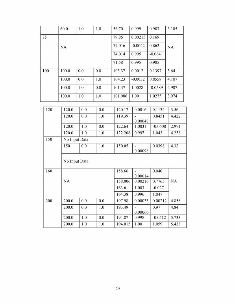
60.0 1.0 1.0 56.70 0.999 0.983 3.105

75 NA

79.85 0.00215 0.169 NA 77.016 -0.0042 0.862

74.014 0.995 -0.064

71.58 0.995 0.985

100 100.0 0.0 0.0 103.37 0.0012 0.1397 3.64

100.0 0.0 1.0 104.23 -0.0032 0.8558 4.107

100.0 1.0 0.0 101.37 1.0028 -0.0589 2.907

100.0 1.0 1.0 101.086 1.00 1.0275 3.974

120 120.0 0.0 0.0 120.17 0.0016 0.1134 3.56

120.0 0.0 1.0 119.39 -0.00048

0.8451 4.422

120.0 1.0 0.0 122.64 1.0031 -0.0608 2.971 120.0 1.0 1.0 122.208 0.997 1.043 4.258

150 No Input Data 150 0.0 1.0 150.05 -

0.000980.0398 4.32

No Input Data

160 NA

158.66 -0.00014

0.040 NA 158.006 0.00216 0.7765

163.6 1.003 -0.027 164.38 0.996 1.047

200 200.0 0.0 0.0 197.98 0.00033 0.00212 4.856 200.0 0.0 1.0 193.49 -

0.000660.97 4.84

200.0 1.0 0.0 194.87 0.998 -0.0512 5.733 200.0 1.0 1.0 194.015 1.00 1.059 5.438

30

3. Conclusions: In this pilot study, several scenarios of large break LOCA with and without ECCS have been modeled using artificial neural networks. The LOCA in RIH with ECCS, RIH without ECCS, and ROH with and without ECCS scenarios have been modeled with individual neural networks. The break sizes ranging from 20% to 200% in reactor headers are considered. A few break sizes were predicted without being trained earlier. The test results obtained from ANN are within the acceptable range. However, it is seen from this pilot study that, artificial neural networks can efficiently predict the unknown break sizes with considerable error. Further, all these previous break scenarios have been modelled with single neural network with three parameters in the output pattern. This study was conducted on different network architectures. The results of two architectures for which the performance was better are presented. The performance of network with two hidden layers is better compared to that of a single layer network. Therefore, this network architecture is adopted for future transient analysis. In future the code will be tested against more number of events and different events with close thermal hydraulic trends will be tested.

References :

1. Safety Analysis Report, Kaiga 3 & 4, NPCIL 2. Computerized Operator Information System (COIS), Kaiga 3 & 4, NPCIL 3. Radiation Data Acquisition System (RADAS), Kaiga 3 & 4, NPCIL. 4. Beetle Monitoring System (BMS), Kaiga 3 & 4, NPCIL 5. Symptom Based Diagnostic System (SBDS) for Kaiga 3 & 4, BARC 6. BIKAS Neural Networks Simulator, Version 7.0.5, 2005, BARC

ANNEXURE – A1 : Description of Computer Codes and Analytical Models of Various Reactor Systems

Various computer codes are used for generating the database for the ANN based computer code as shown in Fig. 1.6. Simulation model has been developed using safety analysis computer code RELAP5/mod3.2 [A1.1] for core thermal-hydraulics, PHTACT [A1.2] for fission product release from core, SOPHAEROS [A1.3, A1.4] module of code ASTEC for fission product retention in PHT piping, CONTRAN [A1.5] for containment thermal-hydraulics and fission product retention by filters, NAUA Mod 5-M [A1.6] for fission product dispersion in the containment and COSYMA [A1.7] for fission product dispersion to atmosphere and dose evaluation. Following are the brief description of the codes and simulation models. A-1.1 : Computational model for Primary Heat Transport (PHT) System, Secondary System and ECC System (ECCS): 754 MW thermal power produced in the Primary Heat Transport System of 220 MWe, is transferred to the secondary side of the steam generator to generate steam. Simulation model for PHTS, Secondary System and ECC System of 220 MWe PHWR has been developed with safety analysis computer code RELAP5/Mod3.2. to Following section briefs the code and the simulation models. Description of RELAP5/MOD3.2 : The basic field equations for the two-fluid non equilibrium model consist of the two phasic continuity equations, two phasic momentum equations and two phasic energy equations. These equations are formulated in differential stream tube form with time and one space dimension as independent variables and in terms of time and volume-average dependent variables. The heat structure is represented by one-dimensional heat conduction in rectangular, cylindrical, or spherical geometry. This acts as boundary conditions/sink/source. This is used to simulate heat generating sources like nuclear fuel rods, sink like steam generator tubes and boundary conditions like PHT system pipe walls. Finite difference formulation is used to advance the heat conduction solutions. The heat transfer correlation package is being used for heat structure surface connected to hydrodynamic volumes and contains correlations for convective, nucleate boiling, transition boiling and film boiling heat transfer from the wall to water and reverse transfer from water to wall, including condensation. Equilibrium and non-equilibrium models are used to evaluate critical (chocked) flow rates for fluid flow paths. Accumulators, different kinds of valves, centrifugal pumps, turbine can be modelled with the component models which solves different governing equations. Parameters evaluated by the computational tools are fluid pressure, temperature (vapor and liquid), thermodynamic and mass qualities, void fraction (vapor and liquid), phasic flow rates and velocity, sonic velocity, carry over and carry under surface temperatures, heat, pump speed, accumulator levels, flux etc. RELAP5/Mod3.2 Specific PHT and ECC System Model The discretisation of the reactor PHT system is shown in Fig. A1-1. Out of the 153 channels in a pass, 152 channels are clubbed to form an average powered channel and a

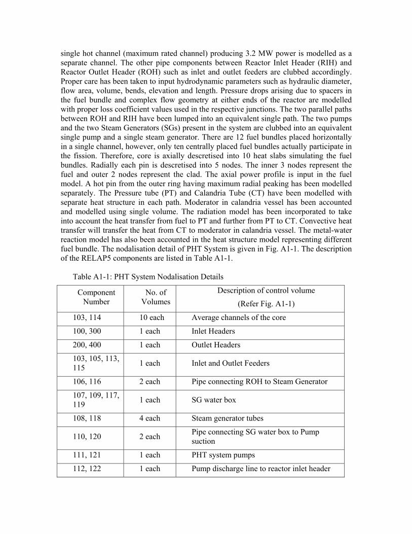
single hot channel (maximum rated channel) producing 3.2 MW power is modelled as a separate channel. The other pipe components between Reactor Inlet Header (RIH) and Reactor Outlet Header (ROH) such as inlet and outlet feeders are clubbed accordingly. Proper care has been taken to input hydrodynamic parameters such as hydraulic diameter, flow area, volume, bends, elevation and length. Pressure drops arising due to spacers in the fuel bundle and complex flow geometry at either ends of the reactor are modelled with proper loss coefficient values used in the respective junctions. The two parallel paths between ROH and RIH have been lumped into an equivalent single path. The two pumps and the two Steam Generators (SGs) present in the system are clubbed into an equivalent single pump and a single steam generator. There are 12 fuel bundles placed horizontally in a single channel, however, only ten centrally placed fuel bundles actually participate in the fission. Therefore, core is axially descretised into 10 heat slabs simulating the fuel bundles. Radially each pin is descretised into 5 nodes. The inner 3 nodes represent the fuel and outer 2 nodes represent the clad. The axial power profile is input in the fuel model. A hot pin from the outer ring having maximum radial peaking has been modelled separately. The Pressure tube (PT) and Calandria Tube (CT) have been modelled with separate heat structure in each path. Moderator in calandria vessel has been accounted and modelled using single volume. The radiation model has been incorporated to take into account the heat transfer from fuel to PT and further from PT to CT. Convective heat transfer will transfer the heat from CT to moderator in calandria vessel. The metal-water reaction model has also been accounted in the heat structure model representing different fuel bundle. The nodalisation detail of PHT System is given in Fig. A1-1. The description of the RELAP5 components are listed in Table A1-1.

Table A1-1: PHT System Nodalisation Details

Component Number

No. of Volumes

Description of control volume

(Refer Fig. A1-1)

103, 114 10 each Average channels of the core

100, 300 1 each Inlet Headers

200, 400 1 each Outlet Headers

103, 105, 113, 115 1 each Inlet and Outlet Feeders

106, 116 2 each Pipe connecting ROH to Steam Generator

107, 109, 117, 119 1 each SG water box

108, 118 4 each Steam generator tubes

110, 120 2 each Pipe connecting SG water box to Pump suction

111, 121 1 each PHT system pumps

112, 122 1 each Pump discharge line to reactor inlet header

100(1)

103(10)

200(1)

107(1) 109(1)

300(1)

117(1) 119(1)

114(10)

400(1)

102(1) 104(1)

106(2)

108(

4)

110(2)

111(1)

112(1)

113(1)115(1)

116(2)

118(

4)

120(2)

121(1)

122(1)

301

302 303

304

305

306

307308

309

312

313

314315

316

317

318

319320

321

322

907

124

957

958

905

123

955

956

906

904

908

959

214(10)

203(10)215(1) 213(1)

202(1)

204(1)327

328329

330

324 325

326323

600Containment

Volume

201Break Junction

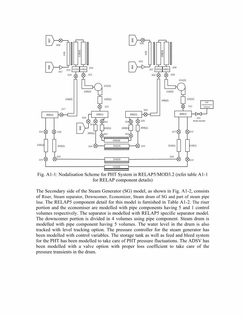
Fig. A1-1: Nodalisation Scheme for PHT System in RELAP5/MOD3.2 (refer table A1-1

for RELAP component details) The Secondary side of the Steam Generator (SG) model, as shown in Fig. A1-2, consists of Riser, Steam separator, Downcomer, Economizer, Steam drum of SG and part of steam pipe line. The RELAP5 component detail for this model is furnished in Table A1-2. The riser portion and the economiser are modelled with pipe components having 5 and 1 control volumes respectively. The separator is modelled with RELAP5 specific separator model. The downcomer portion is divided in 4 volumes using pipe component. Steam drum is modelled with pipe component having 5 volumes. The water level in the drum is also tracked with level tracking option. The pressure controller for the steam generator has been modelled with control variables. The storage tank as well as feed and bleed system for the PHT has been modelled to take care of PHT pressure fluctuations. The ADSV has been modelled with a valve option with proper loss coefficient to take care of the pressure transients in the drum.

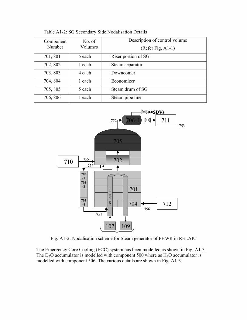
Table A1-2: SG Secondary Side Nodalisation Details

Component Number

No. of Volumes

Description of control volume

(Refer Fig. A1-1)

701, 801 5 each Riser portion of SG

702, 802 1 each Steam separator

703, 803 4 each Downcomer

704, 804 1 each Economizer

705, 805 5 each Steam drum of SG

706, 806 1 each Steam pipe line

701

704 712

703-1

703-2

703-4

108

705

702710

706-1 711

107 109

SDVs

756751

754

755

752753

701

704 712

703-1

703-2

703-4

108

705

702710

706-1 711

107 109

SDVs

756751

754

755

752753

Fig. A1-2: Nodalisation scheme for Steam generator of PHWR in RELAP5

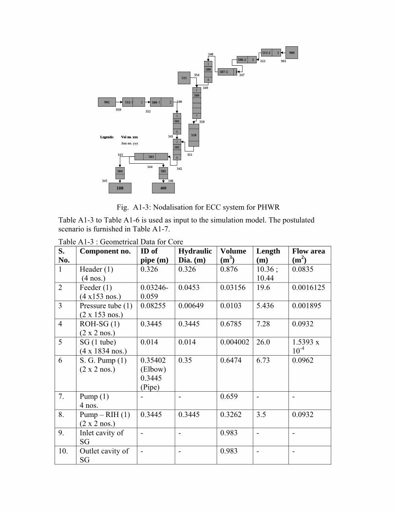
The Emergency Core Cooling (ECC) system has been modelled as shown in Fig. A1-3. The D2O accumulator is modelled with component 500 where as H2O accumulator is modelled with component 506. The various details are shown in Fig. A1-3.

902 512-1 2 500-1 2

900513-2 1

507-5 1

511

100 400

504 505

503

510

1502

4

1501

6

1508

4

1509

7

506-2 1

345 346

344

343

342

341

959 352

340

351

350

354

349

348

347

353 901

Legends: Vol no. xxx

Jun no. yyy

902 512-1 2 500-1 2

900513-2 1

507-5 1

511

100 400

504 505

503

510

1502

4

1501

6

1508

4

1509

7

506-2 1

345 346

344

343

342

341

959 352

340

351

350

354

349

348

347

353 901

Legends: Vol no. xxx

Jun no. yyy

Fig. A1-3: Nodalisation for ECC system for PHWR

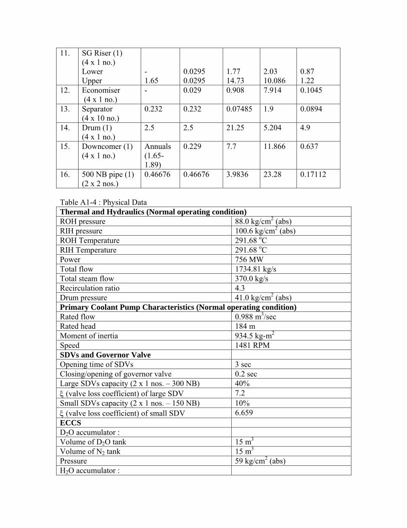
Table A1-3 to Table A1-6 is used as input to the simulation model. The postulated scenario is furnished in Table A1-7.

Table A1-3 : Geometrical Data for Core S. No.

Component no. ID of pipe (m)

Hydraulic Dia. (m)

Volume (m3)

Length (m)

Flow area (m2)

1 Header (1) (4 nos.)

0.326 0.326 0.876 10.36 ; 10.44

0.0835

2 Feeder (1) (4 x153 nos.)

0.03246-0.059

0.0453 0.03156 19.6 0.0016125

3 Pressure tube (1) (2 x 153 nos.)

0.08255 0.00649 0.0103 5.436 0.001895

4 ROH-SG (1) (2 x 2 nos.)

0.3445 0.3445 0.6785 7.28 0.0932

5 SG (1 tube) (4 x 1834 nos.)

0.014 0.014 0.004002 26.0 1.5393 x 10-4

6 S. G. Pump (1) (2 x 2 nos.)

0.35402 (Elbow) 0.3445 (Pipe)

0.35 0.6474 6.73 0.0962

7. Pump (1) 4 nos.

- - 0.659 - -

8. Pump – RIH (1) (2 x 2 nos.)

0.3445 0.3445 0.3262 3.5 0.0932

9. Inlet cavity of SG

- - 0.983 - -

10. Outlet cavity of SG

- - 0.983 - -

11. SG Riser (1) (4 x 1 no.) Lower Upper

- 1.65

0.0295 0.0295

1.77 14.73

2.03 10.086

0.87 1.22

12. Economiser (4 x 1 no.)

- 0.029 0.908 7.914 0.1045

13. Separator (4 x 10 no.)

0.232 0.232 0.07485 1.9 0.0894

14. Drum (1) (4 x 1 no.)

2.5 2.5 21.25 5.204 4.9

15. Downcomer (1) (4 x 1 no.)

Annuals (1.65-1.89)

0.229 7.7 11.866 0.637

16. 500 NB pipe (1) (2 x 2 nos.)

0.46676 0.46676 3.9836 23.28 0.17112

Table A1-4 : Physical Data Thermal and Hydraulics (Normal operating condition)ROH pressure 88.0 kg/cm2 (abs) RIH pressure 100.6 kg/cm2 (abs) ROH Temperature 291.68 oC RIH Temperature 291.68 oC Power 756 MW Total flow 1734.81 kg/s Total steam flow 370.0 kg/s Recirculation ratio 4.3 Drum pressure 41.0 kg/cm2 (abs) Primary Coolant Pump Characteristics (Normal operating condition) Rated flow 0.988 m3/sec Rated head 184 m Moment of inertia 934.5 kg-m2 Speed 1481 RPM SDVs and Governor Valve Opening time of SDVs 3 sec Closing/opening of governor valve 0.2 sec Large SDVs capacity (2 x 1 nos. – 300 NB) 40% ξ (valve loss coefficient) of large SDV 7.2 Small SDVs capacity (2 x 1 nos. – 150 NB) 10% ξ (valve loss coefficient) of small SDV 6.659 ECCS D2O accumulator : Volume of D2O tank 15 m3 Volume of N2 tank 15 m3 Pressure 59 kg/cm2 (abs) H2O accumulator :

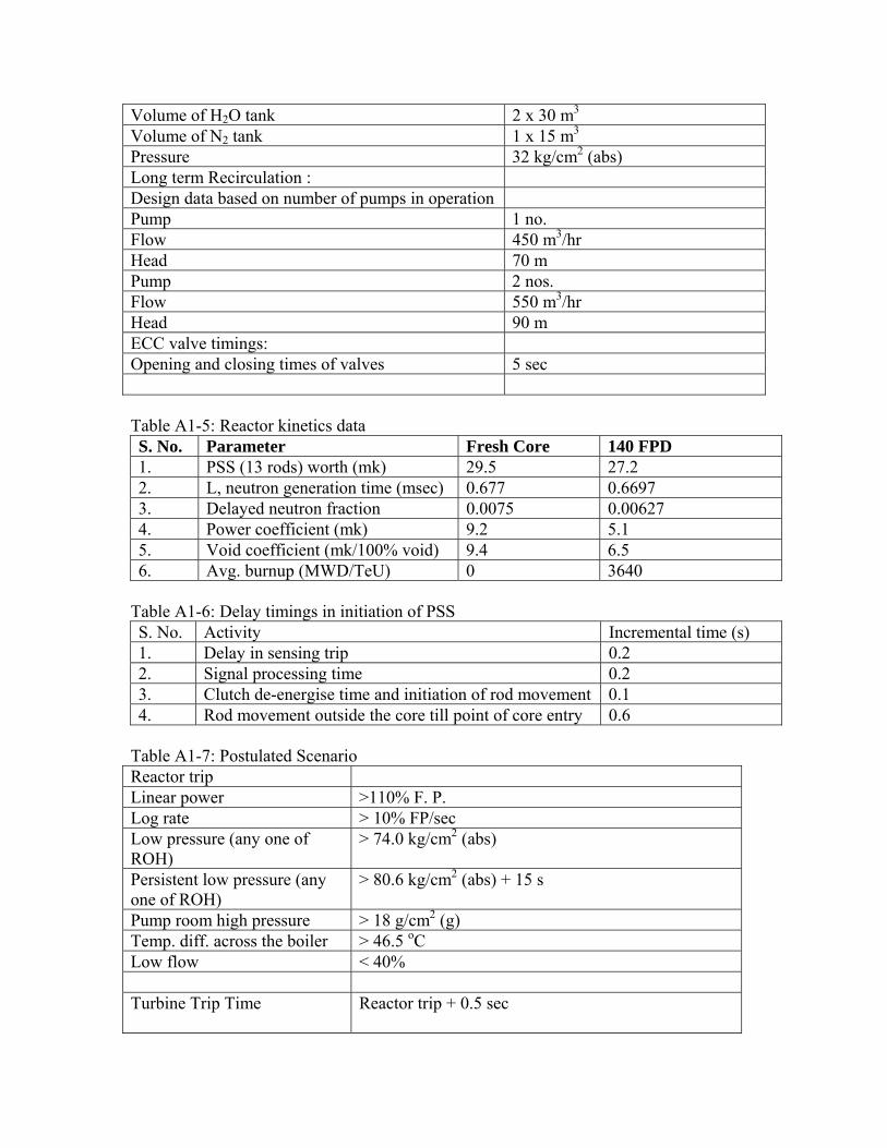
Volume of H2O tank 2 x 30 m3 Volume of N2 tank 1 x 15 m3 Pressure 32 kg/cm2 (abs) Long term Recirculation : Design data based on number of pumps in operation Pump 1 no. Flow 450 m3/hr Head 70 m Pump 2 nos. Flow 550 m3/hr Head 90 m ECC valve timings: Opening and closing times of valves 5 sec

Table A1-5: Reactor kinetics data S. No. Parameter Fresh Core 140 FPD 1. PSS (13 rods) worth (mk) 29.5 27.2 2. L, neutron generation time (msec) 0.677 0.6697 3. Delayed neutron fraction 0.0075 0.00627 4. Power coefficient (mk) 9.2 5.1 5. Void coefficient (mk/100% void) 9.4 6.5 6. Avg. burnup (MWD/TeU) 0 3640

Table A1-6: Delay timings in initiation of PSS S. No. Activity Incremental time (s)1. Delay in sensing trip 0.2 2. Signal processing time 0.2 3. Clutch de-energise time and initiation of rod movement 0.1 4. Rod movement outside the core till point of core entry 0.6

Table A1-7: Postulated Scenario Reactor trip Linear power >110% F. P. Log rate > 10% FP/sec Low pressure (any one of ROH)

> 74.0 kg/cm2 (abs)

Persistent low pressure (any one of ROH)

> 80.6 kg/cm2 (abs) + 15 s

Pump room high pressure > 18 g/cm2 (g) Temp. diff. across the boiler > 46.5 oC Low flow < 40% Turbine Trip Time Reactor trip + 0.5 sec

SDVs opening Opens on pump room high pressure Main coolant pump trip time Pressurising Pump trip + 15 secs Trips with Class IV power failure Pressurising pump trip Storage Tank level low (20 cms, i.e. 0.5 tonnes hold

up) ECCS injection logics D2O injection initiation at RIH pressure

< 56.0 kg/cm2 (abs)

Injection Isolation on D2O accumulator volume and Pressure in D2O accumulator

< 2.75 m3 < 33 kg/cm2 (a)

H2O injection initiation at RIH pressure

< 33 kg/cm2 (a)

A-1.2: Computational model for Containment System (Thermal Hydraulic and Fission Product Transport) The transient pressure and temperature in the containment following the discharge of coolant due to a LOCA have been evaluated using the in-house computer code CONTRAN (CONtainment TRansient ANalysis). Following is a brief description of the code: (1) It is a multicompartment containment transient analysis code which solves the mass

and energy conservation equations within each of the compartments to predict the thermal hydraulic transients.

(2) The code can accomodate any number of compartment and at present each compartment can have six junctions which may act as inlet or outlet depending on the pressure gradient.

(3) Each compartment can have upto three heat slabs of different materials which act as heat sink.

(4) A number of condensation heat transfer coefficient models are available to evalaute heat transfer to containment structures.

(5) 1-D conduction heat transfer model with option of using uniform as well as non-uniform grid sizes is available.

(6) It contains a model to evaluate vent clearing transients in the suppression pool [A1.8].

(7) It has an option of using variable time step for computation. (8) Containment Engineered safety systems such as PCFPB, SCFRP and PCCD can be

modelled.

(9) The blowdown mass and energy discharge rates for any given break size are given as inputs to the code and the post accident containment pressure and temperature transients are the outputs of the code.

(10) Time dependent activity release into the containment can be given as input and ground and stack level release from the containment can be evaluated.

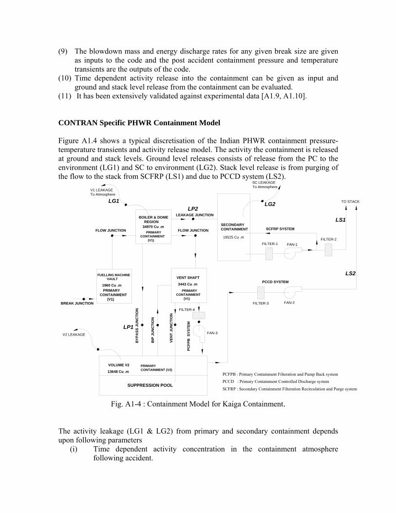
(11) It has been extensively validated against experimental data [A1.9, A1.10]. CONTRAN Specific PHWR Containment Model Figure A1.4 shows a typical discretisation of the Indian PHWR containment pressure-temperature transients and activity release model. The activity the containment is released at ground and stack levels. Ground level releases consists of release from the PC to the environment (LG1) and SC to environment (LG2). Stack level release is from purging of the flow to the stack from SCFRP (LS1) and due to PCCD system (LS2).

FLOW JUNCTIONFLOW JUNCTIONSECONDARY CONTAINMENT SCFRP SYSTEM

BIP

JU

NC

TIO

N

BYP

ASS

JU

NC

TIO

N

VEN

T JU

NC

TIO

N

PCFP

B S

YSTE

M

PCCD SYSTEM

SUPPRESSION POOL

13648 Cu .m

VOLUME V2

V2 LEAKAGE

PRIMARY CONTAINMENT (V2)

FAN-3

FILTER-3 FAN-2

VENT SHAFTFUELLING MACHINE VAULT


BREAK JUNCTION

1960 Cu .m

FILTER-4


3443 Cu .m

PRIMARY CONTAINMENT (V1) FILTER-2

FILTER-1

19525 Cu .m

FAN-1

V1 LEAKAGETo Atmosphere

BOILER & DOME REGION

34970 Cu .m

LEAKAGE JUNCTION

SC LEAKAGETo Atmosphere

TO STACK

PCFPB : Primary Containment Filteration and Pump Back system

PCCD : Primary Containment Controlled Discharge system

SCFRP : Secondary Containment Filteration Recirculation and Purge system

LG1 LG2

LS1

LS2

LP2

LP1

Fig. A1-4 : Containment Model for Kaiga Containment.

The activity leakage (LG1 & LG2) from primary and secondary containment depends upon following parameters

(i) Time dependent activity concentration in the containment atmosphere following accident.

(ii) Time dependent pressure in the containment because leakage rate depends upon the differential pressure between the containment and the atmosphere.

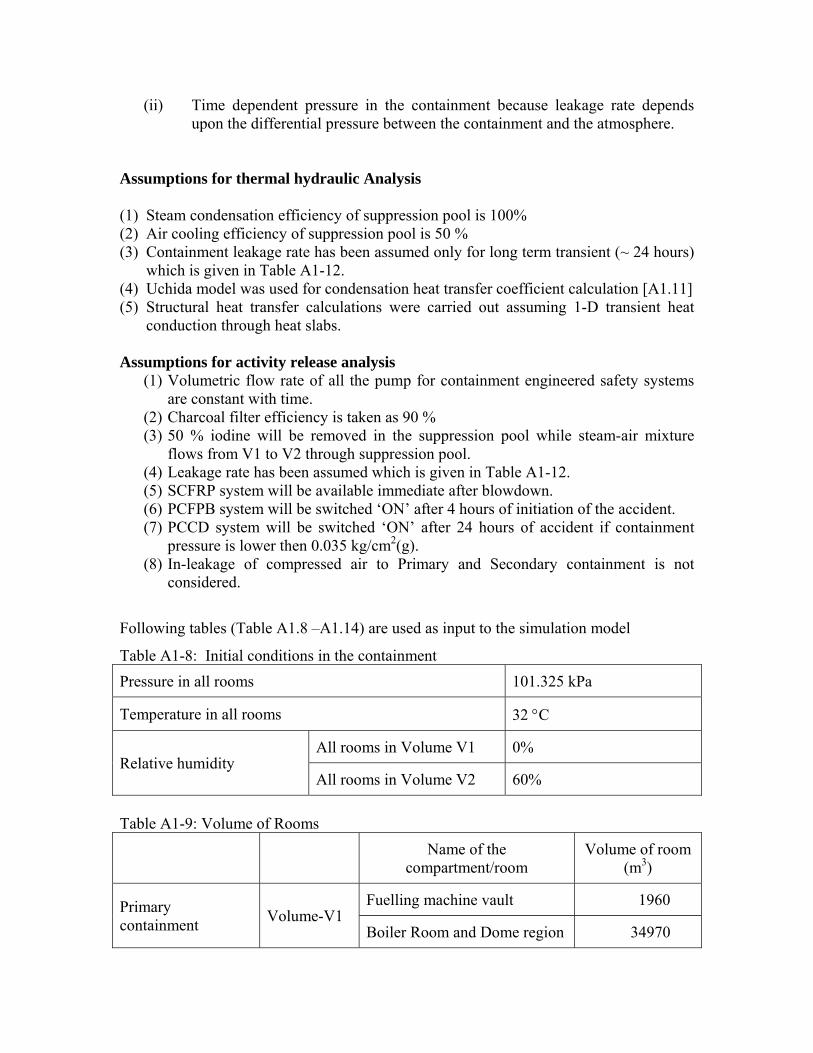
Assumptions for thermal hydraulic Analysis (1) Steam condensation efficiency of suppression pool is 100% (2) Air cooling efficiency of suppression pool is 50 % (3) Containment leakage rate has been assumed only for long term transient (~ 24 hours)

which is given in Table A1-12. (4) Uchida model was used for condensation heat transfer coefficient calculation [A1.11] (5) Structural heat transfer calculations were carried out assuming 1-D transient heat

conduction through heat slabs. Assumptions for activity release analysis

(1) Volumetric flow rate of all the pump for containment engineered safety systems are constant with time.

(2) Charcoal filter efficiency is taken as 90 % (3) 50 % iodine will be removed in the suppression pool while steam-air mixture

flows from V1 to V2 through suppression pool. (4) Leakage rate has been assumed which is given in Table A1-12. (5) SCFRP system will be available immediate after blowdown. (6) PCFPB system will be switched ‘ON’ after 4 hours of initiation of the accident. (7) PCCD system will be switched ‘ON’ after 24 hours of accident if containment

pressure is lower then 0.035 kg/cm2(g). (8) In-leakage of compressed air to Primary and Secondary containment is not

considered.

Following tables (Table A1.8 –A1.14) are used as input to the simulation model

Table A1-8: Initial conditions in the containment Pressure in all rooms 101.325 kPa

Temperature in all rooms 32 °C

Relative humidity All rooms in Volume V1 0%

All rooms in Volume V2 60% Table A1-9: Volume of Rooms

Name of the compartment/room

Volume of room (m3)

Primary containment Volume-V1

Fuelling machine vault 1960

Boiler Room and Dome region 34970

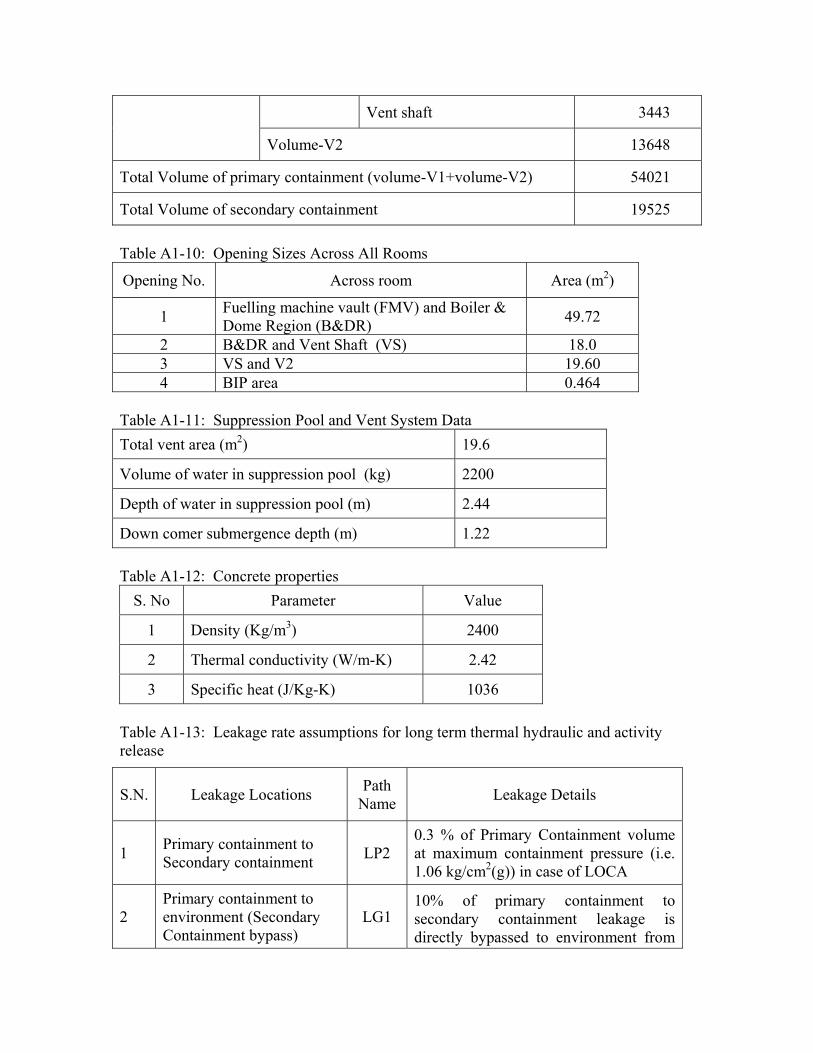
Vent shaft 3443

Volume-V2 13648

Total Volume of primary containment (volume-V1+volume-V2) 54021

Total Volume of secondary containment 19525 Table A1-10: Opening Sizes Across All Rooms

Opening No. Across room Area (m2)

1 Fuelling machine vault (FMV) and Boiler & Dome Region (B&DR) 49.72

2 B&DR and Vent Shaft (VS) 18.0 3 VS and V2 19.60 4 BIP area 0.464

Table A1-11: Suppression Pool and Vent System Data Total vent area (m2) 19.6

Volume of water in suppression pool (kg) 2200

Depth of water in suppression pool (m) 2.44

Down comer submergence depth (m) 1.22 Table A1-12: Concrete properties

S. No Parameter Value

1 Density (Kg/m3) 2400

2 Thermal conductivity (W/m-K) 2.42

3 Specific heat (J/Kg-K) 1036 Table A1-13: Leakage rate assumptions for long term thermal hydraulic and activity release

S.N. Leakage Locations Path Name Leakage Details

1 Primary containment to Secondary containment LP2

0.3 % of Primary Containment volume at maximum containment pressure (i.e. 1.06 kg/cm2(g)) in case of LOCA

2 Primary containment to environment (Secondary Containment bypass)

LG1 10% of primary containment to secondary containment leakage is directly bypassed to environment from

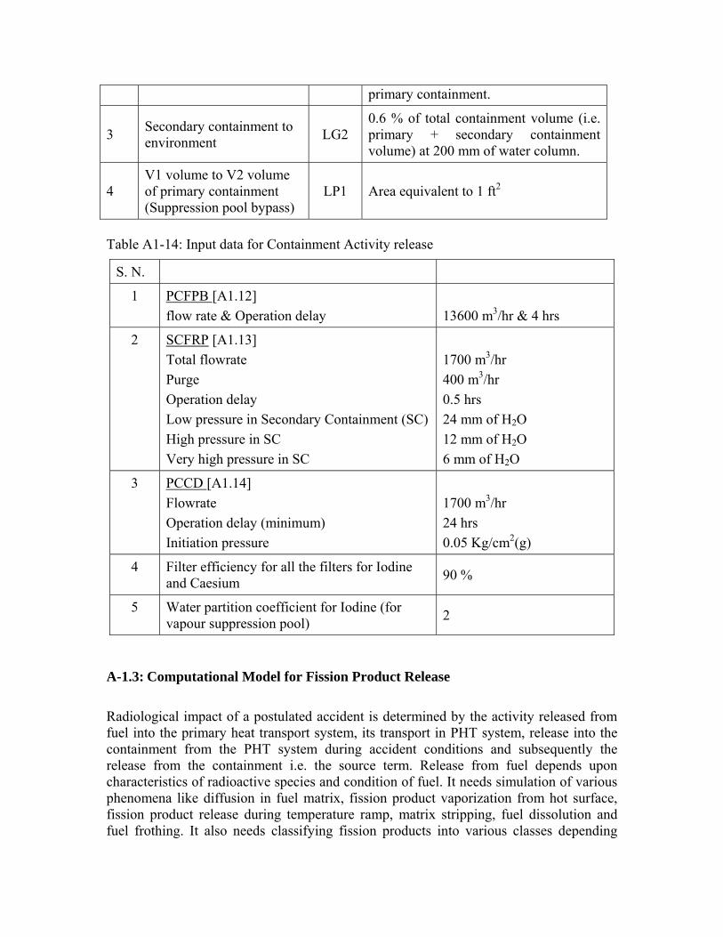
primary containment.

3 Secondary containment to environment LG2

0.6 % of total containment volume (i.e. primary + secondary containment volume) at 200 mm of water column.

4 V1 volume to V2 volume of primary containment (Suppression pool bypass)

LP1 Area equivalent to 1 ft2

Table A1-14: Input data for Containment Activity release

S. N.

1 PCFPB [A1.12] flow rate & Operation delay

13600 m3/hr & 4 hrs

2 SCFRP [A1.13] Total flowrate Purge Operation delay Low pressure in Secondary Containment (SC) High pressure in SC Very high pressure in SC

1700 m3/hr 400 m3/hr 0.5 hrs 24 mm of H2O 12 mm of H2O 6 mm of H2O

3 PCCD [A1.14] Flowrate Operation delay (minimum) Initiation pressure

1700 m3/hr 24 hrs 0.05 Kg/cm2(g)

4 Filter efficiency for all the filters for Iodine and Caesium 90 %

5 Water partition coefficient for Iodine (for vapour suppression pool) 2

A-1.3: Computational Model for Fission Product Release

Radiological impact of a postulated accident is determined by the activity released from fuel into the primary heat transport system, its transport in PHT system, release into the containment from the PHT system during accident conditions and subsequently the release from the containment i.e. the source term. Release from fuel depends upon characteristics of radioactive species and condition of fuel. It needs simulation of various phenomena like diffusion in fuel matrix, fission product vaporization from hot surface, fission product release during temperature ramp, matrix stripping, fuel dissolution and fuel frothing. It also needs classifying fission products into various classes depending

upon chemical and physical characteristics, volatility, and affinity to zirconium. Based on these phenomena and species characteristics large numbers of mechanistic models are developed. There are also empirical model based on experimental data. Pioneering work among these is NUREG – 0772 [A1.15] fission release model, which is also referred as bounding model by many researchers. Based on both mechanistic and non-mechanistic models large numbers of code are developed for light water reactors [A1.16, A1.17, A1.18]. However, these codes do not take into account PHWR geometry. A computer code PHTACT is developed that take into account variation of different power in different fuel rods, flow stratification in channel, sagging and ballooning of channels. Fission products release is calculated based on correlation used in NUREG – 0772 which is still used by many researchers as a bounding model. The code PHTACT is developed in such a way that it can be used to different accident scenario in PHWR. The fission product release model takes into account 14 major fission products. ELOCA.Mk6 is one such computer code used for CANDU analysis [A1.19, A1.20]

The code needs plant specific information like initial species inventory and their distribution in different channels at different nodes. It also needs accident specific information like time history of fuel average temperature at various nodes, time profiles for fluid mass inventories and fluid flow rates in different control volumes and junctions and inter connection of different control volumes. The code computes release rates as a function of time for different species groups in different core volumes, distribution of each species in PHT system and release into the containment.

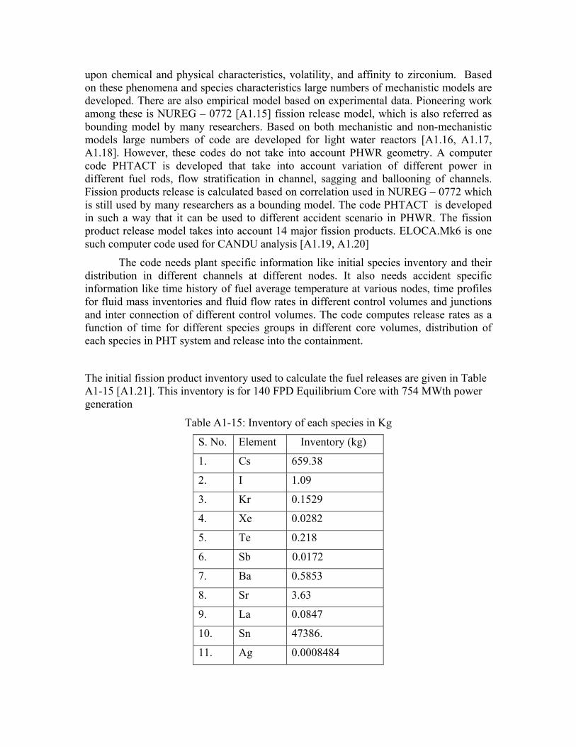
The initial fission product inventory used to calculate the fuel releases are given in Table A1-15 [A1.21]. This inventory is for 140 FPD Equilibrium Core with 754 MWth power generation

Table A1-15: Inventory of each species in Kg

S. No. Element Inventory (kg)

1. Cs 659.38

2. I 1.09

3. Kr 0.1529

4. Xe 0.0282

5. Te 0.218

6. Sb 0.0172

7. Ba 0.5853

8. Sr 3.63

9. La 0.0847

10. Sn 47386.

11. Ag 0.0008484

12. Zr 0.1029

13. Mo 0.0856

14. Ru 1.215

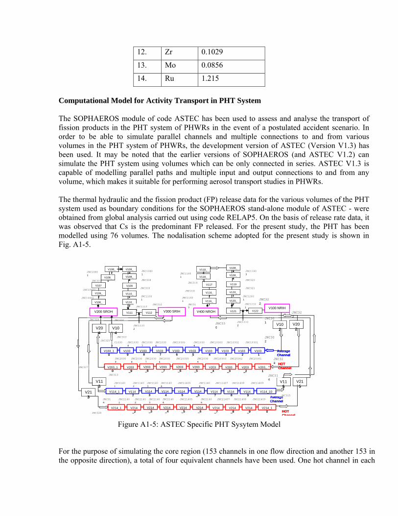
Computational Model for Activity Transport in PHT System The SOPHAEROS module of code ASTEC has been used to assess and analyse the transport of fission products in the PHT system of PHWRs in the event of a postulated accident scenario. In order to be able to simulate parallel channels and multiple connections to and from various volumes in the PHT system of PHWRs, the development version of ASTEC (Version V1.3) has been used. It may be noted that the earlier versions of SOPHAEROS (and ASTEC V1.2) can simulate the PHT system using volumes which can be only connected in series. ASTEC V1.3 is capable of modelling parallel paths and multiple input and output connections to and from any volume, which makes it suitable for performing aerosol transport studies in PHWRs.

The thermal hydraulic and the fission product (FP) release data for the various volumes of the PHT system used as boundary conditions for the SOPHAEROS stand-alone module of ASTEC - were obtained from global analysis carried out using code RELAP5. On the basis of release rate data, it was observed that Cs is the predominant FP released. For the present study, the PHT has been modelled using 76 volumes. The nodalisation scheme adopted for the present study is shown in Fig. A1-5.

Figure A1-5: ASTEC Specific PHT Sysytem Model For the purpose of simulating the core region (153 channels in one flow direction and another 153 in the opposite direction), a total of four equivalent channels have been used. One hot channel in each

JNC305

JNC327

JNC302

V103_1

V103_2

V103_3

V103_4

V103_5

V103_6

V103_7

V103_8

V103_9

V103_10

JNC10301JNC10302JNC10303JNC10304

JNC10305JNC10306

JNC10307

JNC10308

JNC10309

V104

JNC303

V200 SROH

JNC304

V203_1

V203_2

V203_3

V203_4

V203_5

V203_6

V203_7

V203_8

V203_9

V203_10

JNC20301JNC20302JNC20303JNC20304

JNC20305JNC20306

JNC20307

JNC20308

JNC20309

JNC324

V204

JNC325

JNC326

JNC10602

JNC307

JNC10601

V106_1

V106_2

V107

V108_1

V108_2

V112

V108_3

V108_4

V109

V110_1

V110_2

V111 V300 SRIHV100 NRIH

V102

JNC301

JNC323

V202

JNC330

V108_3

V108_4

V119

V120_1

V120_2

V121 V122V400 NROH

V116_1

V116_2

V117

V118_1

V118_2

V114_10V114_9

V114_8

V114_7

V114_6

V114_5

V114_4

V114_3

V114_2

V114_1

JNC11409JNC11408JNC11407JNC11406

JNC11405JNC11404

JNC11403

JNC11402

JNC11401

V214_10

V214_9

V214_8

V214_7

V214_6

V214_5

V214_4

V214_3

V214_2

V214_1

JNC21409JNC21408JNC21407JNC21406

JNC21405JNC21404

JNC21403

JNC21402

JNC21401

JNC313

V113

V213

JNC314

JNC328

V115

JNC316 V21

5

JNC315

JNC320

JNC12001

JNC12102

JNC11601

JNC317

JNC11801

JNC318

JNC11803

JNC321

JNC319

JNC12101

JNC322

JNC10801

JNC10801

JNC308

JNC309

JNC11001

JNC11101

JNC11102

JNC312

HOT Channel

Average Channel

HOT Channel

Average Channel

JNC305

JNC327

JNC302

V103_1

V103_2

V103_3

V103_4

V103_5

V103_6

V103_7

V103_8

V103_9

V103_10

JNC10301JNC10302JNC10303JNC10304

JNC10305JNC10306

JNC10307

JNC10308

JNC10309

V104

JNC303

V200 SROH

JNC304

V203_1

V203_2

V203_3

V203_4

V203_5

V203_6

V203_7

V203_8

V203_9

V203_10

JNC20301JNC20302JNC20303JNC20304

JNC20305JNC20306

JNC20307

JNC20308

JNC20309

JNC324

V204

JNC325

JNC326

JNC10602

JNC307

JNC10601

V106_1

V106_2

V107

V108_1

V108_2

V106_1

V106_2

V107

V108_1

V108_2

V112

V108_3

V108_4

V109

V110_1

V110_2

V111

V108_3

V108_4

V109

V110_1

V110_2

V111 V300 SRIHV100 NRIH

V102

JNC301

JNC323

V202

JNC330

V108_3

V108_4

V119

V120_1

V120_2

V121

V108_3

V108_4

V119

V120_1

V120_2

V121 V122V400 NROH

V116_1

V116_2

V117

V118_1

V118_2

V114_10V114_9

V114_8

V114_7

V114_6

V114_5

V114_4

V114_3

V114_2

V114_1

JNC11409JNC11408JNC11407JNC11406

JNC11405JNC11404

JNC11403

JNC11402

JNC11401

V214_10

V214_9

V214_8

V214_7

V214_6

V214_5

V214_4

V214_3

V214_2

V214_1

JNC21409JNC21408JNC21407JNC21406

JNC21405JNC21404

JNC21403

JNC21402

JNC21401

JNC313

V113

V213

JNC314

JNC328

V115

JNC316 V21

5

JNC315

JNC320

JNC12001

JNC12102

JNC11601

JNC317

JNC11801

JNC318

JNC11803

JNC321

JNC319

JNC12101

JNC322

JNC10801

JNC10801

JNC308

JNC309

JNC11001

JNC11101

JNC11102

JNC312

HOT Channel

Average Channel

HOT Channel

Average Channel

pass represents 23 maximum rated power channel of the core and the other channel (average rated channel) represents a channel with average power corresponding to the remaining 130 pairs of channels. Each of these four channels is divided into ten volumes of equal length. The four headers are modelled as one volume each. The actual number of steam generators in the PHT loop is four (two on each pass). For ASTEC, the two steam generators in one pass have been modelled as a single steam generator with geometrical and thermal hydraulic data corresponding to two steam generators. Each such steam generator is modelled by using four volumes. The injection of fission products is assumed in the central volume of the maximum rated channel corresponding to V214_5 and V203_5. A-1.4 : Description of Code NAUA and Containment Aerosol Dispersion Model : The NAUA code [A1.22] simulates coagulation, sedimentation, diffusional deposition and steam condensation on particles. The code uses a numerical representation of the particle size distribution. Thermal hydraulic data must be supplied as input to the code. An extension of the original version is NAUA Mod 5-M for multiple compartment geometries, where the NAUA aerosol simulations are performed for several control volumes. In addition, advective flows between different control volumes are taken into account. Thermal hydraulic conditions and inter compartment flow rates have to be specified as input data. Thus, NAUA requires the operation of an extra code for containment thermal hydraulics, and does not take into account possible feedback effects which aerosols may cause in the thermal hydraulic conditions. The following simplifying assumptions are made in the code NAUA (i) Particles are homogeneously distributed in a control volume except for the boundary layer at the walls (ii) Within one particle size class, no difference in particle composition is allowed (iii) Particle properties like density may change due to varying moisture content of the particle (iv) Shape factor and boundary layer thickness are assumed to be independent of particle size. Internal mixing of species within a size class is assumed to be quickly achieved by coagulation. The spatial homogeneity in the control volume is generally considered to be accomplished by natural convection within the control volume.

The code models gravitational deposition and diffusional plate-out as the removal mechanisms. The removal of aerosol by inertial, electrostatic and thermophoretic processes is not considered. Among the aerosol interaction processes, the code considers Brownian coagulation, gravitational agglomeration, and aerosol growth by steam condensation. The code uses a constant diffusional boundary layer thickness of 0.01 cm. The particle dimension used is the volume equivalent radius, which for normal applications is equivalent to Stokes' radius [A1.6]. Although the code has provision for arbitrary shape factor values, the shape factors for condensation, mobility and agglomeration are normally set at unity, which is approximately true for accidents in water-cooled reactors. The porosity of the water-logged spherical agglomerates is accounted for by using an effective density equal to 50% of the actual value. As the code

is not integrated with the containment thermal hydraulics, the condensation rates for condensation on particles and the internal wall surfaces are required to be specified as input quantities. NAUA can follow the build up of up to 50 nuclide species on a size independent basis. The minimum particle size normally handled is 0.01 μm and the maximum size is 100 μm. This range can be accommodated in up to 101 size classes. Particle concentrations up to 10-14 cc -1 can be considered. It is a discrete code, in which although the input may be in any form (tabular or log-normal distribution), the particles are subsequently tracked using only the total number of size classes and the upper and lower size limit values. This is unlike the log-normal codes, where it is assumed .that the size distribution at the end of a time step remains log-normal. Aerosol and steam rates, containment dimensions and containment thermodynamics, and the leak rate are inputs to the code. The code output includes time-dependent air-borne mass concentration, cumulative amounts removed by diffusion, sedimentation, leakage, and the information on particle size and size distribution. The code NAUA is a well validated code, both at the level of separate effect experiments in the small NAUA vessel at KfK as also in the integral tests in the Battelle-Frankfurt's DEMONA (Demonstration of Behavior of Nuclear Aerosols) facility. NAUA is regarded as one of the most tested and used mechanistic containment codes for aerosol behavior analysis. A NAUA-specific PHWR containment model has been developed. The model consists of Volume V1 and V2 connected by VENT junction. The Volume connectivity and geometric parameters used in the calculation are shown in Fig. A-1.6. For the PHWR containment the aerosol source available from PHTACT was injected in volume V1. The aerosol injection period was divided into 22 release phases each phase being characterized by uniform values of release rate, effective density, particle size characteristics, and nuclide compositions. The effective density was the mass-averaged density for each release phase. Two radionuclide species Cs-137 and I-131 were considered. Though the source of iodine is small but it is enough from radiation point of view. The Mass median diameter of particle log normal distribution was 4 μm and geometric standard deviation was 1.9. The particle density was assumed as 1.1 gm/cc. Thermodynamic parameters like containment gas temperature, partial pressure of steam and air in all the volumes obtained by CONTRAN as an input to code NAUA5-M. Volumetric flow rate through junction between volumes and volume connectivity was also provided to NAUA5-M.

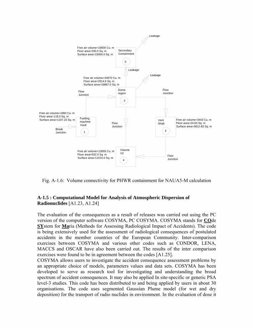
Fuelling machine Vault

1Break Junction

Vent Shaft

3

2

Dome region

Secondary Containment

5

Volume V2

4

Flow Junction

Flow Junction

Flow Junction

Flow Junction

Leakage

Leakage

Leakage

Free air volume=3443 Cu. mFloor area=24.63 Sq. mSurface area=5812.83 Sq. m





Fig. A-1.6: Volume connectivity for PHWR containment for NAUA5-M calculation A-1.5 : Computational Model for Analysis of Atmospheric Dispersion of Radionuclides [A1.23, A1.24] The evaluation of the consequences as a result of releases was carried out using the PC version of the computer software COSYMA, PC COSYMA. COSYMA stands for COde SYstem for Maria (Methods for Assessing Radiological Impact of Accidents). The code is being extensively used for the assessment of radiological consequences of postulated accidents in the member countries of the European Community. Inter-comparison exercises between COSYMA and various other codes such as CONDOR, LENA, MACCS and OSCAR have also been carried out. The results of the inter comparison exercises were found to be in agreement between the codes [A1.25]. COSYMA allows users to investigate the accident consequence assessment problems by an appropriate choice of models, parameters values and data sets. COSYMA has been developed to serve as research tool for investigating and understanding the broad spectrum of accident consequences. It may also be applied In site-specific or generic PSA level-3 studies. This code has been distributed to and being applied by users in about 30 organisations. The code uses segmented Gaussian Plume model (for wet and dry deposition) for the transport of radio nuclides in environment. In the evaluation of dose it

considers contribution of inhalation, skin deposition, ingestion and ground contamination. Doses to various organs such as bone marrow, thyroid, eye lenses are the outputs the code provides. Like any other Probabilistic Consequence Assessment (PCA) code, COSYMA also has models for atmospheric dispersion and deposition, meteorological sampling, dose assessment through exposure pathways, countermeasures, health effects and economic consequences. It needs as input description of radionuclide release data (fission product transient release from ground and stack), meteorological data (wind velocity, stability category, precipitation rate, inversion layer thickness), dose conversion factors, risk conversion factors, economic data if economic consequences are to be evaluated and population and agricultural data in case risk to the public is needed. The pathways considered in COSYMA are: i) external irradiation from radioactive material in the passing plume or cloud of

radioactive material, referred to as cloud shine; ii) external irradiation from radioactive material deposited on the ground, referred to

as ground shine; iii) external irradiation from radioactive material deposited on the skin and clothing,

generally called contamination; iv) internal irradiation from radioactive material inhaled directly from the passing

plume; v) internal irradiation from radioactive material inhaled following resuspension of

ground deposit; vi) internal irradiation from radioactive material ingested following the direct or

indirect contamination of foodstuffs or drinking water by radioactive material deposited from the plume.

The early fatal health effects are considered from irradiation of the bone marrow (haematopoietic syndrome), the lung (pulmonary syndrome), the GI-tract (gastrointestinal syndrome) and skin (skin burns). In addition, the mortality of pre and neonates after exposure in utero is normally quantified. The occurrences of wide variety of radiation induced injuries like prodromal vomiting, diarrhoea, hypothyroidism, temporary sterility, mental retardation is also investigated by COSYMA. The meteorological data used for the evaluations corresponds to that of KAPS site. Radioactive source term for the evaluations was obtained from the results of multiple code approach as described in Fig. 1.6.

References : [A1.1] Allison, C. M., RELAP/MOD3.2 Code Manual, NUREG/CR-5535, INEL -95/0174, 1995

[A1.2] Lele H.G., Mukhopadhyaya D., Behera, G. , Gupta S.K., “PHTACT – A Computer Code For Estimation Of Fission Product Release And Transport For Pressurised Heavy Water Reactor During Accident Conditions” RSD/CSSS/SKG/2069/2001, Divisional Report, April 2001 [A1.3] J-P Van Dorsselaere, S.Pignet, C.Seropian, T.Montanelli, P.Giordano, F.Jacq, B.Scwhinges, "Development and assessment of ASTEC code for severe Accident simulation", NURETH-11, Avignon, France, October 2-6, 2005 [A1.4] J.P. Van Dorsselaere, J.C. Micaelli, H.J. Allelein, "ASTEC and SARNET - Integrating severe accident research in Europe", ICAPP ’05, Seoul, Korea, May 15-19, 2005 [A1.5] Haware, S. K., Markandeya, S. G., Ghosh, A. K., and Venkat Raj,V., January 1994, “Assessment of multi-compartment containment analysis computer code CONTRAN with the experiments on containment response during LOCA conditions”, First ISHMT-ASME Heat and Mass Transfer Conference and 12th National Heat and Mass Transfer Conference, BARC, Bombay, India.

[A1.6] Bunz, H., Kyoro, M. and Schoeck, W. (1987) NAUA Mod 5 and Mod 5-M, Zwei Computerprogramme zur Berechung des Aerosolverhaltens im Containmentsystem eines LWR nach einem Kernschmelzunfall. KfK-4278, Kernforschungszentrum, Karlsruhe. [A1.7] PC COSYMA Version 2.0 Users Guide, EUR 16240 EN (NRPB-SR280), National Radiological Protection Board, Forschungszentrum Karlsruhe GmbH, November 1995.

[A1.8] Ghosh, A.K., and Grover, R.B, 1984, “Analysis of vent clearing transient in a pressure suppression type containment system”, BARC Report No. BARC/I-814, BARC, Bombay.

[A1.9] Haware, S. K., Ghosh, A. K., Venkat Raj,V., and Kakodkar, A., Oct 1994, “Analysis of CSNI Benchmark test on containment using the code CONTRAN” Third International Conference on Containment Design and Operation, Vol-2, Toronto, Ontario.

[A1.10] S. K. Haware and V. Venkat Raj, August 1989, “Experiments on one-tenth scale model of vapour suppression pool containment of 235MWe Indian PHWRs - Results of one of the tests simulating MAPS condition”, 10th National Heat and Mass Transfer Conference, Aug 23-25, 1989, Srinagar, India.

[A1.11] Almenas, K., July 1982, “Heat transfer from saturated and superheated atmospheres for containment analysis”, Nucl. Eng. Des. 71 (1), 1-14

[A1.12] Nuclear Power Corporation of India Limited, Mumbai, India, “Design Manual on Reactor Building Primary Containment Filtration and Pump Back system”, Kaiga-1&2-73150.

[A1.13] Nuclear Power Corporation of India Limited, Mumbai, India, “Design Manual on Reactor Building Secondary Containment Ventilation, Filtration and Purge system”, Kaiga-1&2-73160.

[A1.14] Nuclear Power Corporation of India Limited, Mumbai, India, “Design Manual on Reactor Building Primary Containment Controlled Depressurisation System”, RAPP-3&4-73140-2.

[A1.15] US NRC, Technical Basis for Estimation of Fission Product Behaviour for LWR accidents, NUREG-0772, June 1981. [A1.16] H. Manenc, M. P. Kissane, P. Giordano, ESCARDE mos1.2, ELSA Code Version1.1 rev1 : Fission Product Release from the Reactor Core, Technical Note IPSN/DRS/SEMAR 98/97 [A1.17] Rest, J., Zawadzki, S.A. FASTGRASS, A Mechanistic Model for the Prediction of Xe, I, Cs, Te, Ba and Sr release from Nuclear Fuel under Normal and Severe-Accident Conditions, NUREG/CR-5840 TI92 040783, 1994. [A1.18] Heames et al., T.J. VICTORIA: A Mechanistic Model of Radionuclide Behavior in the Reactor Coolant System Under Severe Accident Conditions, NUREG/CR-5545 SAND90-0756 Rev 1R3, R4, 1992. [A1.19] H.E. Sills, “ELOCA Fuel Element Behaviour during LOCA,” AECL Report, AECL-6357, 1980. [A1.20] L.D. MacDonald, D.B. Duncan, B.J. Lewis and F.C. Iglesias, “FREEDOM: A Transient Fission-Product Release Model for Radioactive and Stable Species”, AECL Report AECL-98 10, 1988. [A1.21] Safety Analysis Report for Kaiga, Volume –II [A1.22] Bunz, H., Kyoro, M. And Schoeck, W. (1983) NAUA-4: ACode for calculating Aerosol Behaviour in LWR Core Melt Accidents, Kfk-3554, Kernforschungszentrum, Karlsruhe [A1.23] Manual of Dose Evaluation from Atmospheric Releases, R.K. Hukkoo, V.N. Bapat and V.V. Shirvaikar, BARC-1412, 1988 [A1.24] 10th BARC – NPCIL Wrokshop on Planning Preparedness and Response to Radiological Emergencies for DAE Officials at RAPS, Kota, February 05-09, 2001,

Lecture notes compiled and edited by P.S. Sivasubramanian, R.K. Verma and Anil A. Shanbag [A1.25] Probabilistic Accident Consequence Assessment Codes, Second International Comparison, Technical Report, EUR 15109 EN, 1994.

ANNEXURE – A2 : Accident Analysis and Generation of Data Base

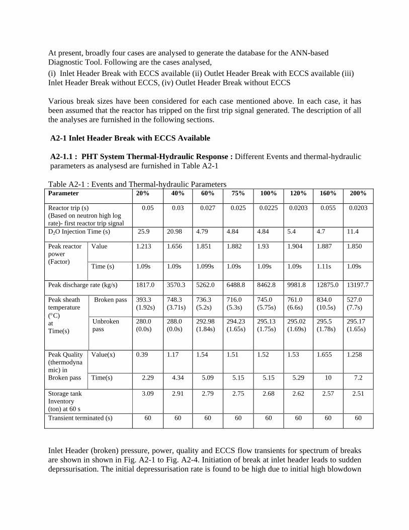
At present, broadly four cases are analysed to generate the database for the ANN-based Diagnostic Tool. Following are the cases analysed, (i) Inlet Header Break with ECCS available (ii) Outlet Header Break with ECCS available (iii) Inlet Header Break without ECCS, (iv) Outlet Header Break without ECCS Various break sizes have been considered for each case mentioned above. In each case, it has been assumed that the reactor has tripped on the first trip signal generated. The description of all the analyses are furnished in the following sections. A2-1 Inlet Header Break with ECCS Available A2-1.1 : PHT System Thermal-Hydraulic Response : Different Events and thermal-hydraulic parameters as analysesd are furnished in Table A2-1 Table A2-1 : Events and Thermal-hydraulic Parameters Parameter 20% 40% 60% 75% 100% 120% 160% 200%

Reactor trip (s) (Based on neutron high log rate)- first reactor trip signal

0.05 0.03 0.027 0.025 0.0225 0.0203 0.055 0.0203

D2O Injection Time (s) 25.9 20.98 4.79 4.84 4.84 5.4 4.7 11.4

Peak reactor power (Factor)

Value 1.213 1.656 1.851 1.882 1.93 1.904 1.887

1.850

Time (s) 1.09s 1.09s 1.099s 1.09s 1.09s 1.09s 1.11s 1.09s

Peak discharge rate (kg/s) 1817.0 3570.3 5262.0 6488.8 8462.8 9981.8 12875.0 13197.7

Peak sheath temperature (°C) at Time(s)

Broken pass

393.3 (1.92s)

748.3 (3.71s)

736.3 (5.2s)

716.0 (5.3s)

745.0 (5.75s)

761.0 (6.6s)

834.0 (10.5s)

527.0 (7.7s)

Unbroken pass

280.0 (0.0s)

288.0 (0.0s)

292.98 (1.84s)

294.23 (1.65s)

295.13 (1.75s)

295.02 (1.69s)

295.5 (1.78s)

295.17 (1.65s)

Peak Quality (thermodynamic) in Broken pass

Value(x) 0.39 1.17 1.54 1.51 1.52 1.53 1.655 1.258

Time(s) 2.29 4.34 5.09 5.15 5.15 5.29 10 7.2

Storage tank Inventory (ton) at 60 s

3.09 2.91 2.79 2.75 2.68 2.62 2.57 2.51

Transient terminated (s) 60 60 60 60 60 60 60 60

Inlet Header (broken) pressure, power, quality and ECCS flow transients for spectrum of breaks are shown in shown in Fig. A2-1 to Fig. A2-4. Initiation of break at inlet header leads to sudden deprssurisation. The initial depressurisation rate is found to be high due to initial high blowdown

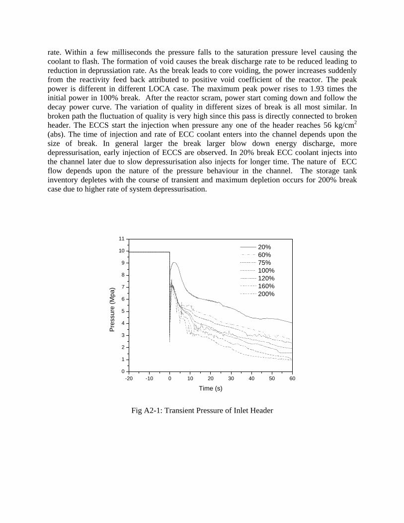
rate. Within a few milliseconds the pressure falls to the saturation pressure level causing the coolant to flash. The formation of void causes the break discharge rate to be reduced leading to reduction in deprussiation rate. As the break leads to core voiding, the power increases suddenly from the reactivity feed back attributed to positive void coefficient of the reactor. The peak power is different in different LOCA case. The maximum peak power rises to 1.93 times the initial power in 100% break. After the reactor scram, power start coming down and follow the decay power curve. The variation of quality in different sizes of break is all most similar. In broken path the fluctuation of quality is very high since this pass is directly connected to broken header. The ECCS start the injection when pressure any one of the header reaches 56 kg/cm2 (abs). The time of injection and rate of ECC coolant enters into the channel depends upon the size of break. In general larger the break larger blow down energy discharge, more depressurisation, early injection of ECCS are observed. In 20% break ECC coolant injects into the channel later due to slow depressurisation also injects for longer time. The nature of ECC flow depends upon the nature of the pressure behaviour in the channel. The storage tank inventory depletes with the course of transient and maximum depletion occurs for 200% break case due to higher rate of system depressurisation.

-20 -10 0 10 20 30 40 50 600

1

2

3

4

5

6

7

8

9

10

11

20% 60% 75% 100% 120% 160% 200%

Pre

ssur

e (M

pa)

Time (s)

Fig A2-1: Transient Pressure of Inlet Header

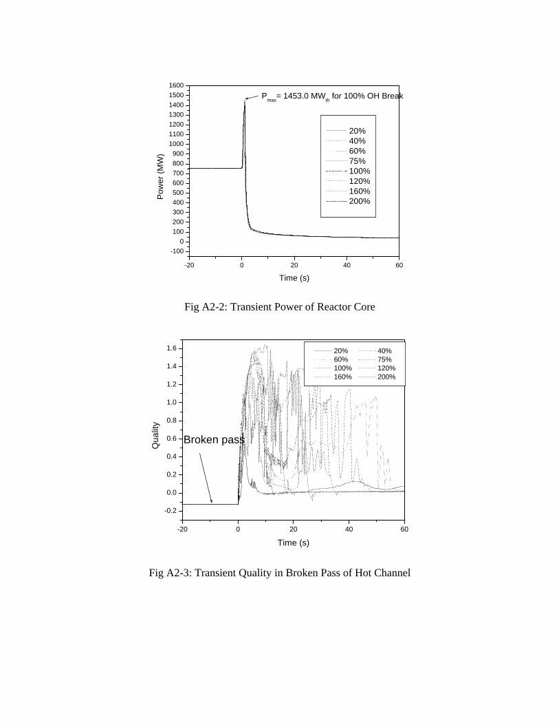
-20 0 20 40 60

-1000

100200300400500600700800900

1000110012001300140015001600

Pmax= 1453.0 MWth for 100% OH Break

Pow

er (M

W)

Time (s)

20% 40% 60% 75% 100% 120% 160% 200%

Fig A2-2: Transient Power of Reactor Core

-20 0 20 40 60

-0.2

0.0

0.2

0.4

0.6

0.8

1.0

1.2

1.4

1.6 20% 40% 60% 75% 100% 120% 160% 200%

Broken pass

Qua

lity

Time (s)

Fig A2-3: Transient Quality in Broken Pass of Hot Channel

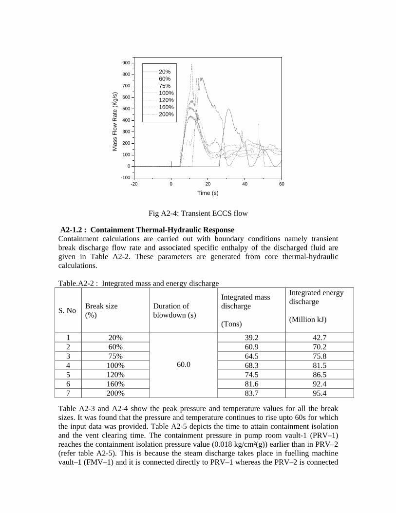
-20 0 20 40 60-100

0

100

200

300

400

500

600

700

800

900

Mas

s Fl

ow R

ate

(Kg/

s)

Time (s)

20% 60% 75% 100% 120% 160% 200%

Fig A2-4: Transient ECCS flow

A2-1.2 : Containment Thermal-Hydraulic Response Containment calculations are carried out with boundary conditions namely transient break discharge flow rate and associated specific enthalpy of the discharged fluid are given in Table A2-2. These parameters are generated from core thermal-hydraulic calculations. Table.A2-2 : Integrated mass and energy discharge

S. No Break size (%)

Duration of blowdown (s)

Integrated mass discharge (Tons)

Integrated energy discharge (Million kJ)

1 20%

60.0

39.2 42.7 2 60% 60.9 70.2 3 75% 64.5 75.8 4 100% 68.3 81.5 5 120% 74.5 86.5 6 160% 81.6 92.4 7 200% 83.7 95.4

Table A2-3 and A2-4 show the peak pressure and temperature values for all the break sizes. It was found that the pressure and temperature continues to rise upto 60s for which the input data was provided. Table A2-5 depicts the time to attain containment isolation and the vent clearing time. The containment pressure in pump room vault-1 (PRV–1) reaches the containment isolation pressure value (0.018 kg/cm²(g)) earlier than in PRV–2 (refer table A2-5). This is because the steam discharge takes place in fuelling machine vault–1 (FMV–1) and it is connected directly to PRV–1 whereas the PRV–2 is connected

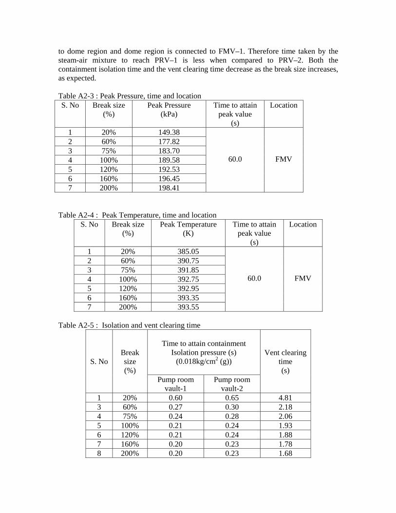
to dome region and dome region is connected to FMV–1. Therefore time taken by the steam-air mixture to reach PRV–1 is less when compared to PRV–2. Both the containment isolation time and the vent clearing time decrease as the break size increases, as expected. Table A2-3 : Peak Pressure, time and location S. No Break size

(%) Peak Pressure

(kPa) Time to attain

peak value (s)

Location

1 20% 149.38

60.0

FMV

2 60% 177.82 3 75% 183.70 4 100% 189.58 5 120% 192.53 6 160% 196.45 7 200% 198.41

Table A2-4 : Peak Temperature, time and location


Peak Temperature (K)

Time to attain peak value

(s)

Location

1 20% 385.05

60.0

FMV

2 60% 390.75 3 75% 391.85 4 100% 392.75 5 120% 392.95 6 160% 393.35 7 200% 393.55

Table A2-5 : Isolation and vent clearing time


Time to attain containment

Isolation pressure (s) (0.018kg/cm2 (g))

Vent clearing time (s)

Pump room vault-1

Pump room vault-2

1 20% 0.60 0.65 4.81 3 60% 0.27 0.30 2.18 4 75% 0.24 0.28 2.06 5 100% 0.21 0.24 1.93 6 120% 0.21 0.24 1.88 7 160% 0.20 0.23 1.78 8 200% 0.20 0.23 1.68

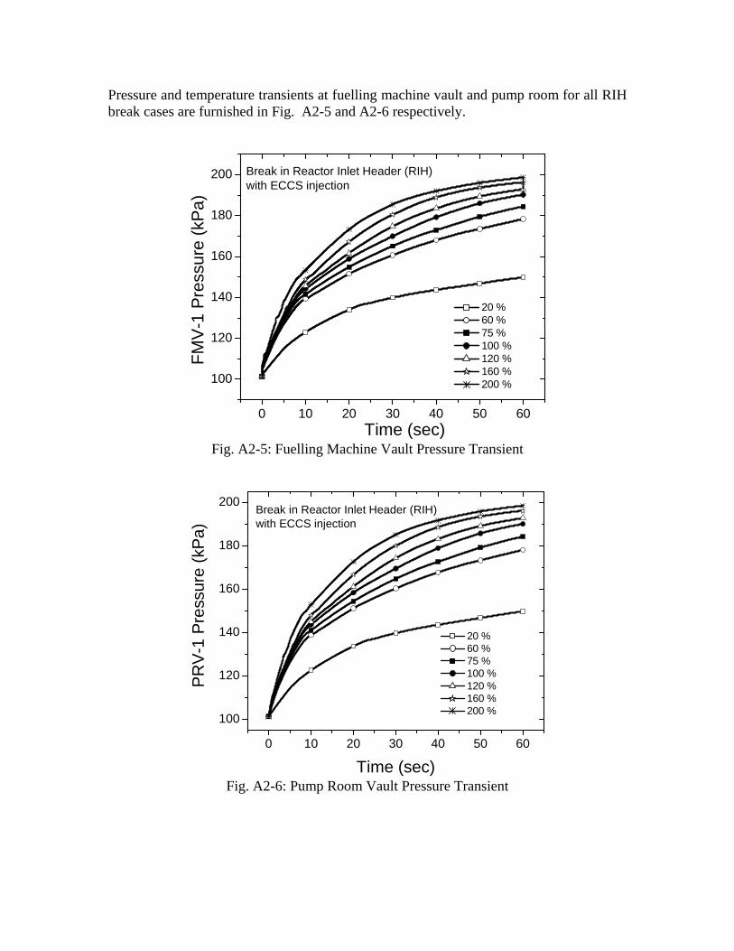
Pressure and temperature transients at fuelling machine vault and pump room for all RIH break cases are furnished in Fig. A2-5 and A2-6 respectively.

0 10 20 30 40 50 60

100

120

140

160

180

200 Break in Reactor Inlet Header (RIH)with ECCS injection

20 % 60 % 75 % 100 % 120 % 160 % 200 %

FMV-

1 Pr

essu

re (k

Pa)

Time (sec) Fig. A2-5: Fuelling Machine Vault Pressure Transient

0 10 20 30 40 50 60

100

120

140

160

180

200Break in Reactor Inlet Header (RIH)with ECCS injection

20 % 60 % 75 % 100 % 120 % 160 % 200 %

PRV-

1 Pr

essu

re (k

Pa)

Time (sec) Fig. A2-6: Pump Room Vault Pressure Transient

A2-2 Outlet Header Break with ECCS Available A2-2.1 : PHT System Thermal-Hydraulic Response Different Events and thermal-hydraulic parameters as analyzed are furnished in Table A2-6 Table A2-6 : Events and Thermal-hydraulic Parameters Parameter 20% 40% 60% 75% 100% 120% 160% 200%


0.08 0.07 0.06 0.08 0.08 0.08 0.07 0.07

D2O accumulator triggered(s)

82.0 37.0 19.79 17.4 15.0 13.7 11.7 10.79

Type-II/III latch(s) 95.5 46.5 26.9 23.79 21.5 66.0 42.0 36.5

Peak reactor power (normalised)

Value 1.011 1.029 1.042 1.04 1.071 1.08 1.09

1.12

Time(s) 0.84s 1.0s 1.05s 0.94s 1.07s 1.05s 1.06s 1.07s

Peak discharge rate (kg/sec) 744.0 1773.0 2839 3633.0 4903.0 5807.0 7376.0 8178.0

Peak sheath temperature (Deg. C) And at Time(s)

Broken pass

288.0C (0.0s)

288.0 (0.0s)

288.0 (0.0s)

288.0 (0.0s)

288.0 (0.0s)

288.0 (0.0s)

288.0 (0.0s)

288.0 (0.0s)

Unbroken pass

290.46 (1.5s)

291.0 (1.7s)

297.19 (73.0s)

297.0 (60.0s)

353.9 (4.8s)

408.1 (4.6s)

521.0 (3.79s)

558.2 (3.70s)

Broken Header Pressure (kg/sq. cm2 ) At 60s

49.60 43.44 39.0 25.3 18.47 17.4 13.92

8.0


Value(x) 0.16 0.71 0.60 0.68 0.48 0.45 0.087 0.28

Time(s) 160.0 108.0 85 65 106 98 31 15.59

Storage tank Inventory (ton) at the end of the transient

3.09

3.01 2.90 2.85 2.73 2.68 2.59 2.5

Transient terminated (s) 160 160 160 160 160 160 160 160

Outlet Header (broken) pressure, power, quality and ECCS flow transients for spectrum of breaks are shown in shown in Fig. A2-7 to Fig. A2-10. The rate of decrease of the pressure of break volume depends on the size the break. The larger the break size greater the fall of pressure and vice-versa. In all the case energy discharge from the break volume is higher than the energy generation in the core results decrease the pressure in the PHT continuous in the transients. The power increases suddenly after the break. The break leads to voided conditions in the core. The positive void reactivity feedback gives rise to increase in the reactivity leading to high power rise. The peak power is different in different LOCA cases. The maximum pick power rises to 1.12 times the initial power in

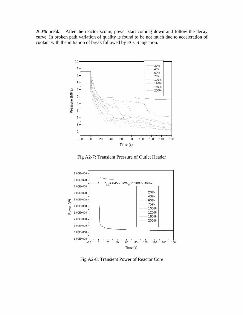
200% break. After the reactor scram, power start coming down and follow the decay curve. In broken path variation of quality is found to be not much due to acceleration of coolant with the initiation of break followed by ECCS injection.

-20 0 20 40 60 80 100 120 140 160

0

1

2

3

4

5

6

7

8

9

10 20% 40% 60% 75% 100% 120% 160% 200%

Pre

ssur

e (M

Pa)

Time (s)

Fig A2-7: Transient Pressure of Outlet Header

-20 0 20 40 60 80 100 120 140 160-1.00E+008

0.00E+000

1.00E+008

2.00E+008

3.00E+008

4.00E+008

5.00E+008

6.00E+008

7.00E+008

8.00E+008

9.00E+008

Pmax= 845.75MWth in 200% Break

Pow

er (W

)

Time (s)

20% 40% 60% 75% 100% 120% 160% 200%

Fig A2-8: Transient Power of Reactor Core

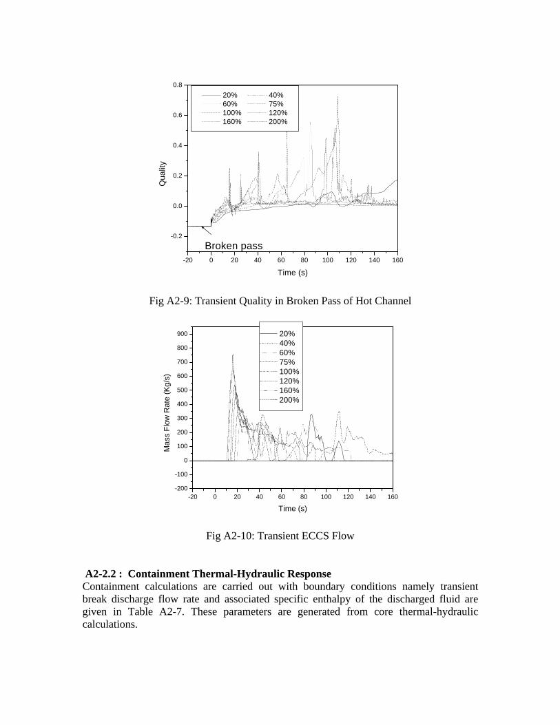
-20 0 20 40 60 80 100 120 140 160

-0.2

0.0

0.2

0.4

0.6

0.8 20% 40% 60% 75% 100% 120% 160% 200%

Broken pass

Qua

lity

Time (s)

Fig A2-9: Transient Quality in Broken Pass of Hot Channel

-20 0 20 40 60 80 100 120 140 160-200

-100

0

100

200

300

400

500

600

700

800

900

Mas

s Fl

ow R

ate

(Kg/

s)

Time (s)

20% 40% 60% 75% 100% 120% 160% 200%

Fig A2-10: Transient ECCS Flow

A2-2.2 : Containment Thermal-Hydraulic Response Containment calculations are carried out with boundary conditions namely transient break discharge flow rate and associated specific enthalpy of the discharged fluid are given in Table A2-7. These parameters are generated from core thermal-hydraulic calculations.

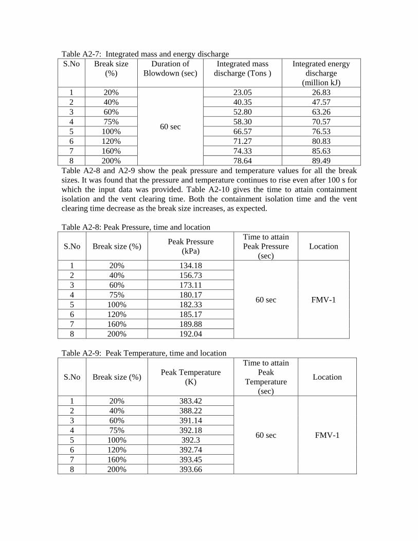
Table A2-7: Integrated mass and energy discharge S.No Break size

(%) Duration of

Blowdown (sec) Integrated mass

discharge (Tons ) Integrated energy

discharge (million kJ)

1 20%

60 sec

23.05 26.83 2 40% 40.35 47.57 3 60% 52.80 63.26 4 75% 58.30 70.57 5 100% 66.57 76.53 6 120% 71.27 80.83 7 160% 74.33 85.63 8 200% 78.64 89.49

Table A2-8 and A2-9 show the peak pressure and temperature values for all the break sizes. It was found that the pressure and temperature continues to rise even after 100 s for which the input data was provided. Table A2-10 gives the time to attain containment isolation and the vent clearing time. Both the containment isolation time and the vent clearing time decrease as the break size increases, as expected. Table A2-8: Peak Pressure, time and location

S.No Break size (%) Peak Pressure (kPa)

Time to attain Peak Pressure

(sec) Location

1 20% 134.18

60 sec FMV-1

2 40% 156.73 3 60% 173.11 4 75% 180.175 100% 182.33 6 120% 185.17 7 160% 189.88 8 200% 192.04

Table A2-9: Peak Temperature, time and location

S.No Break size (%) Peak Temperature (K)

Time to attain Peak

Temperature (sec)

Location

1 20% 383.42

60 sec FMV-1

2 40% 388.22 3 60% 391.14 4 75% 392.18 5 100% 392.3 6 120% 392.74 7 160% 393.458 200% 393.66

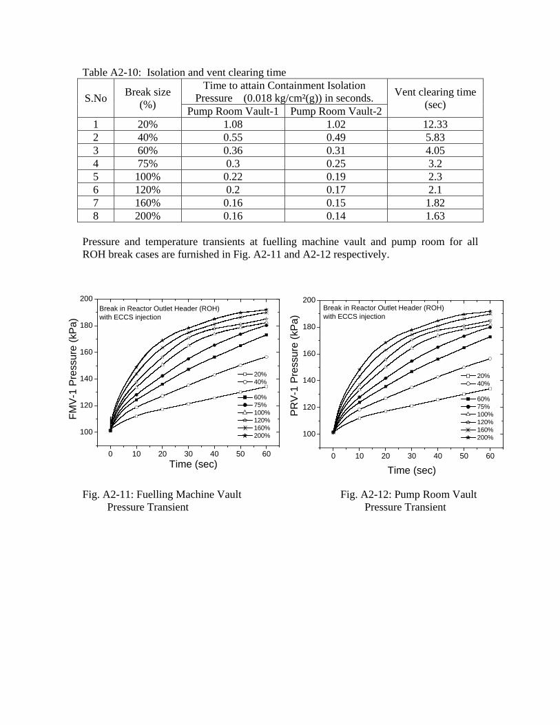
0 10 20 30 40 50 60

100

120

140

160

180

200Break in Reactor Outlet Header (ROH)with ECCS injection

20% 40%

60% 75% 100% 120% 160% 200%

FMV-

1 Pr

essu

re (k

Pa)

Time (sec)0 10 20 30 40 50 60

100

120

140

160

180

200Break in Reactor Outlet Header (ROH)with ECCS injection

20% 40%

60% 75% 100% 120% 160% 200%

PRV-

1 Pr

essu

re (k

Pa)

Time (sec)

Table A2-10: Isolation and vent clearing time

S.No Break size (%)

Time to attain Containment Isolation Pressure (0.018 kg/cm²(g)) in seconds. Vent clearing time

(sec) Pump Room Vault-1 Pump Room Vault-21 20% 1.08 1.02 12.33 2 40% 0.55 0.49 5.83 3 60% 0.36 0.31 4.05 4 75% 0.3 0.25 3.2 5 100% 0.22 0.19 2.3 6 120% 0.2 0.17 2.1 7 160% 0.16 0.15 1.82 8 200% 0.16 0.14 1.63

Pressure and temperature transients at fuelling machine vault and pump room for all ROH break cases are furnished in Fig. A2-11 and A2-12 respectively.

Fig. A2-11: Fuelling Machine Vault Fig. A2-12: Pump Room Vault

Pressure Transient Pressure Transient

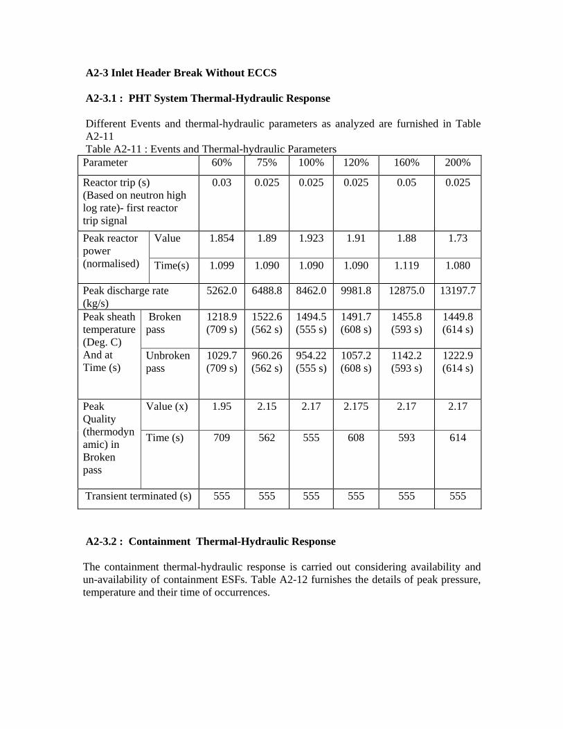
A2-3 Inlet Header Break Without ECCS A2-3.1 : PHT System Thermal-Hydraulic Response Different Events and thermal-hydraulic parameters as analyzed are furnished in Table A2-11 Table A2-11 : Events and Thermal-hydraulic Parameters Parameter 60% 75% 100% 120% 160% 200%


0.03 0.025 0.025 0.025 0.05 0.025

Peak reactor power (normalised)

Value 1.854 1.89 1.923 1.91 1.88

1.73

Time(s) 1.099 1.090 1.090 1.090 1.119 1.080

Peak discharge rate (kg/s)

5262.0 6488.8 8462.0 9981.8 12875.0 13197.7

Peak sheath temperature (Deg. C) And at Time (s)

Broken pass

1218.9 (709 s)

1522.6 (562 s)

1494.5 (555 s)

1491.7 (608 s)

1455.8 (593 s)

1449.8 (614 s)

Unbroken pass

1029.7 (709 s)

960.26 (562 s)

954.22 (555 s)

1057.2 (608 s)

1142.2 (593 s)

1222.9 (614 s)


Value (x) 1.95 2.15 2.17 2.175 2.17 2.17

Time (s) 709 562 555 608 593 614

Transient terminated (s) 555 555 555 555 555 555

A2-3.2 : Containment Thermal-Hydraulic Response The containment thermal-hydraulic response is carried out considering availability and un-availability of containment ESFs. Table A2-12 furnishes the details of peak pressure, temperature and their time of occurrences.

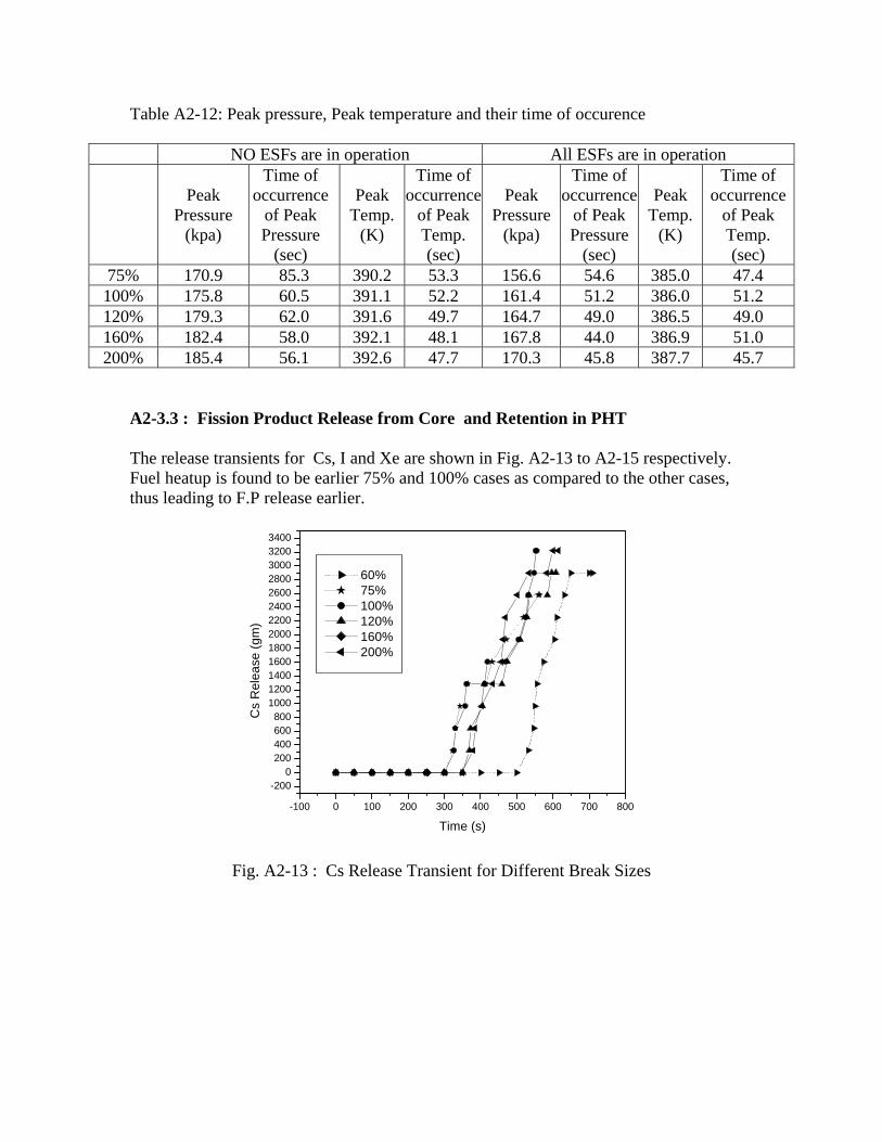
Table A2-12: Peak pressure, Peak temperature and their time of occurence

NO ESFs are in operation All ESFs are in operation

Peak

Pressure (kpa)

Time of occurrence

of Peak Pressure

(sec)

Peak Temp.

(K)

Time of occurrence

of Peak Temp. (sec)

Peak Pressure

(kpa)

Time of occurrence

of Peak Pressure

(sec)

Peak Temp.

(K)

Time of occurrence

of Peak Temp. (sec)

75% 170.9 85.3 390.2 53.3 156.6 54.6 385.0 47.4 100% 175.8 60.5 391.1 52.2 161.4 51.2 386.0 51.2 120% 179.3 62.0 391.6 49.7 164.7 49.0 386.5 49.0 160% 182.4 58.0 392.1 48.1 167.8 44.0 386.9 51.0 200% 185.4 56.1 392.6 47.7 170.3 45.8 387.7 45.7

A2-3.3 : Fission Product Release from Core and Retention in PHT The release transients for Cs, I and Xe are shown in Fig. A2-13 to A2-15 respectively. Fuel heatup is found to be earlier 75% and 100% cases as compared to the other cases, thus leading to F.P release earlier.

-100 0 100 200 300 400 500 600 700 800

-2000

200400600800

1000120014001600180020002200240026002800300032003400

Cs

Rel

ease

(gm

)

Time (s)

60% 75% 100% 120% 160% 200%

Fig. A2-13 : Cs Release Transient for Different Break Sizes

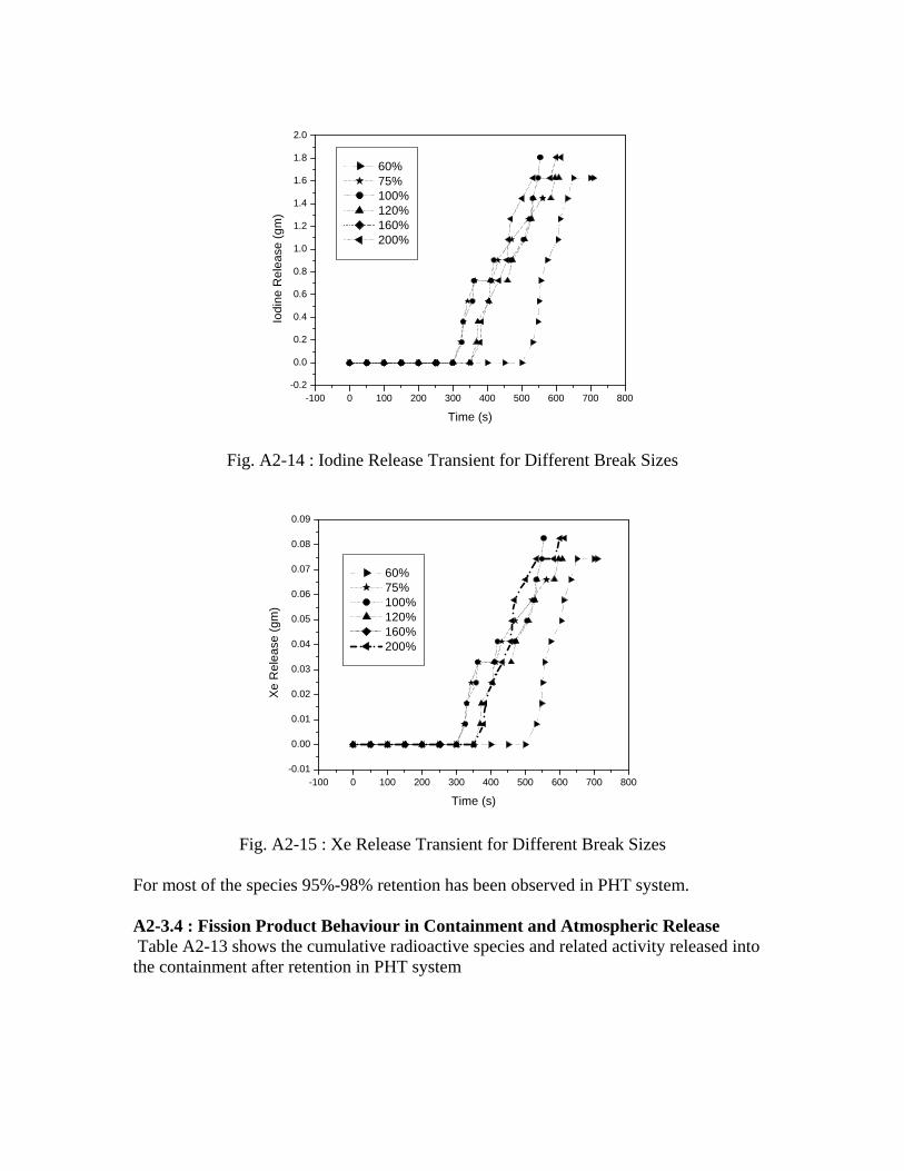
-100 0 100 200 300 400 500 600 700 800-0.2

0.0

0.2

0.4

0.6

0.8

1.0

1.2

1.4

1.6

1.8

2.0

Iodi

ne R

elea

se (g

m)

Time (s)

60% 75% 100% 120% 160% 200%

Fig. A2-14 : Iodine Release Transient for Different Break Sizes

-100 0 100 200 300 400 500 600 700 800-0.01

0.00

0.01

0.02

0.03

0.04

0.05

0.06

0.07

0.08

0.09

Xe R

elea

se (g

m)

Time (s)

60% 75% 100% 120% 160% 200%

Fig. A2-15 : Xe Release Transient for Different Break Sizes

For most of the species 95%-98% retention has been observed in PHT system. A2-3.4 : Fission Product Behaviour in Containment and Atmospheric Release Table A2-13 shows the cumulative radioactive species and related activity released into the containment after retention in PHT system

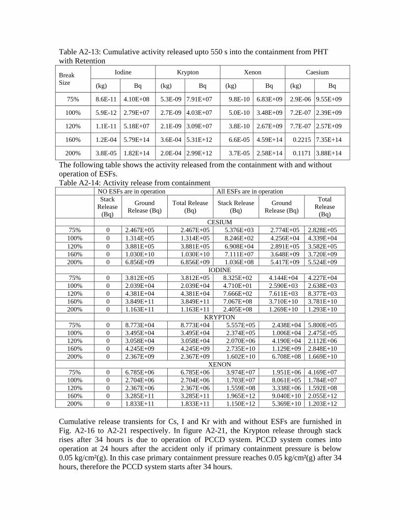
Table A2-13: Cumulative activity released upto 550 s into the containment from PHT with Retention

Break Size

Iodine Krypton Xenon Caesium

(kg) Bq (kg) Bq (kg) Bq (kg) Bq

75% 8.6E-11 4.10E+08 5.3E-09 7.91E+07 9.8E-10 6.83E+09 2.9E-06 9.55E+09

100% 5.9E-12 2.79E+07 2.7E-09 4.03E+07 5.0E-10 3.48E+09 7.2E-07 2.39E+09

120% 1.1E-11 5.18E+07 2.1E-09 3.09E+07 3.8E-10 2.67E+09 7.7E-07 2.57E+09

160% 1.2E-04 5.79E+14 3.6E-04 5.31E+12 6.6E-05 4.59E+14 0.2215 7.35E+14

200% 3.8E-05 1.82E+14 2.0E-04 2.99E+12 3.7E-05 2.58E+14 0.1171 3.88E+14

The following table shows the activity released from the containment with and without operation of ESFs. Table A2-14: Activity release from containment NO ESFs are in operation All ESFs are in operation Stack

Release (Bq)

Ground Release (Bq)

Total Release (Bq)

Stack Release (Bq)

Ground Release (Bq)

Total Release

(Bq) CESIUM

75% 0 2.467E+05 2.467E+05 5.376E+03 2.774E+05 2.828E+05 100% 0 1.314E+05 1.314E+05 8.246E+02 4.256E+04 4.339E+04 120% 0 3.881E+05 3.881E+05 6.908E+04 2.891E+05 3.582E+05 160% 0 1.030E+10 1.030E+10 7.111E+07 3.648E+09 3.720E+09 200% 0 6.856E+09 6.856E+09 1.036E+08 5.417E+09 5.524E+09

IODINE 75% 0 3.812E+05 3.812E+05 8.325E+02 4.144E+04 4.227E+04

100% 0 2.039E+04 2.039E+04 4.710E+01 2.590E+03 2.638E+03 120% 0 4.381E+04 4.381E+04 7.666E+02 7.611E+03 8.377E+03 160% 0 3.849E+11 3.849E+11 7.067E+08 3.710E+10 3.781E+10 200% 0 1.163E+11 1.163E+11 2.405E+08 1.269E+10 1.293E+10

KRYPTON 75% 0 8.773E+04 8.773E+04 5.557E+05 2.438E+04 5.800E+05


XENON 75% 0 6.785E+06 6.785E+06 3.974E+07 1.951E+06 4.169E+07


Cumulative release transients for Cs, I and Kr with and without ESFs are furnished in Fig. A2-16 to A2-21 respectively. In figure A2-21, the Krypton release through stack rises after 34 hours is due to operation of PCCD system. PCCD system comes into operation at 24 hours after the accident only if primary containment pressure is below 0.05 kg/cm²(g). In this case primary containment pressure reaches 0.05 kg/cm²(g) after 34 hours, therefore the PCCD system starts after 34 hours.

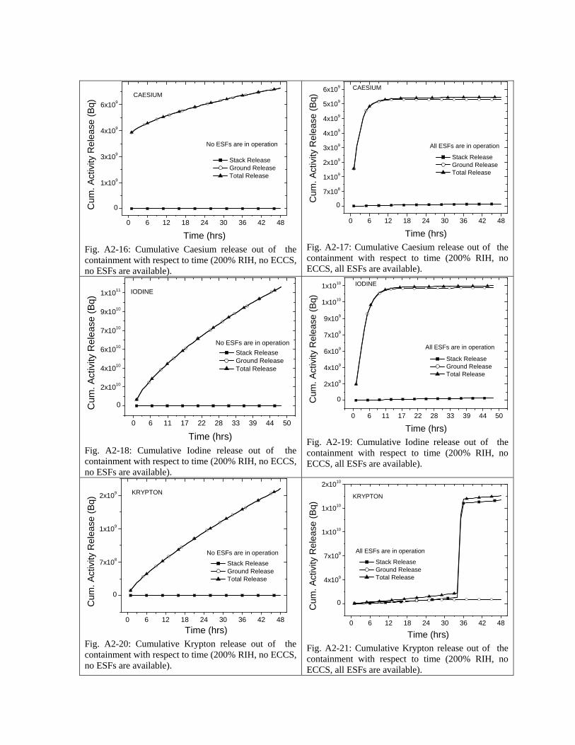
0 6 12 18 24 30 36 42 48

0

1x109

3x109

4x109

6x109

No ESFs are in operation

Stack Release Ground Release Total Release

CAESIUMC

um. A

ctiv

ity R

elea

se (B

q)

Time (hrs) Fig. A2-16: Cumulative Caesium release out of the containment with respect to time (200% RIH, no ECCS, no ESFs are available).

0 6 12 18 24 30 36 42 48

0

7x108

1x109

2x109

3x109

4x109

4x109

5x109

6x109 CAESIUM

All ESFs are in operation


Cum

. Act

ivity

Rel

ease

(Bq)

Time (hrs)Fig. A2-17: Cumulative Caesium release out of the containment with respect to time (200% RIH, no ECCS, all ESFs are available).

0 6 11 17 22 28 33 39 44 50

0

2x1010

4x1010

6x1010

7x1010

9x1010

1x1011 IODINE

No ESFs are in operation Stack Release Ground Release Total Release

Cum

. Act

ivity

Rel

ease

(Bq)

Time (hrs)Fig. A2-18: Cumulative Iodine release out of the containment with respect to time (200% RIH, no ECCS, no ESFs are available).

0 6 11 17 22 28 33 39 44 50

0

2x109

4x109

6x109

7x109

9x109

1x1010

1x1010 IODINE



Cum

. Act

ivity

Rel

ease

(Bq)

Time (hrs) Fig. A2-19: Cumulative Iodine release out of the containment with respect to time (200% RIH, no ECCS, all ESFs are available).

0 6 12 18 24 30 36 42 48

0

7x108

1x109

2x109 KRYPTON

No ESFs are in operation Stack Release Ground Release Total Release

Cum

. Act

ivity

Rel

ease

(Bq)

Time (hrs) Fig. A2-20: Cumulative Krypton release out of the containment with respect to time (200% RIH, no ECCS, no ESFs are available).

0 6 12 18 24 30 36 42 48

0

4x109

7x109

1x1010

1x1010

2x1010

KRYPTON



Cum

. Act

ivity

Rel

ease

(Bq)

Time (hrs) Fig. A2-21: Cumulative Krypton release out of the containment with respect to time (200% RIH, no ECCS, all ESFs are available).

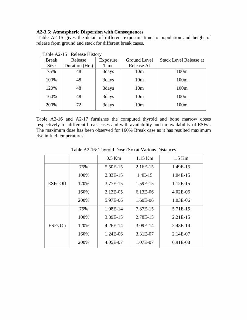
A2-3.5: Atmospheric Dispersion with Consequences Table A2-15 gives the detail of different exposure time to population and height of release from ground and stack for different break cases. Table A2-15 : Release History

Break Size

Release Duration (Hrs)

Exposure Time

Ground Level Release At

Stack Level Release at

75%

100%

120%

160%

200%

48

48

48

48

72

3days

3days

3days

3days

3days

10m

10m

10m

10m

10m

100m

100m

100m

100m

100m

Table A2-16 and A2-17 furnishes the computed thyroid and bone marrow doses respectively for different break cases and with availability and un-availability of ESFs . The maximum dose has been observed for 160% Break case as it has resulted maximum rise in fuel temperatures

Table A2-16: Thyroid Dose (Sv) at Various Distances

0.5 Km 1.15 Km 1.5 Km

ESFs Off

75%

100%

120%

160%

200%

5.50E-15

2.83E-15

3.77E-15

2.13E-05

5.97E-06

2.16E-15

1.4E-15

1.59E-15

6.13E-06

1.60E-06

1.49E-15

1.04E-15

1.12E-15

4.02E-06

1.03E-06

ESFs On

75%

100%

120%

160%

200%

1.08E-14

3.39E-15

4.26E-14

1.24E-06

4.05E-07

7.37E-15

2.78E-15

3.09E-14

3.31E-07

1.07E-07

5.71E-15

2.21E-15

2.43E-14

2.14E-07

6.91E-08

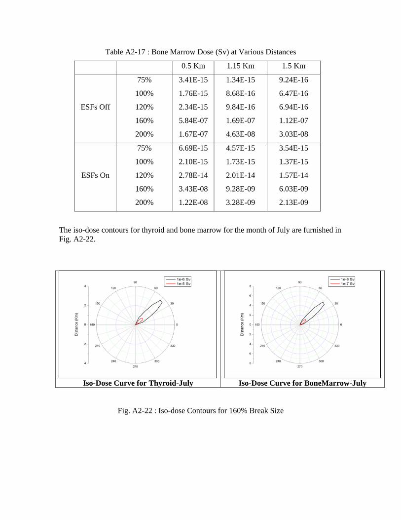
Table A2-17 : Bone Marrow Dose (Sv) at Various Distances

0.5 Km 1.15 Km 1.5 Km

ESFs Off

75%

100%

120%

160%

200%

3.41E-15

1.76E-15

2.34E-15

5.84E-07

1.67E-07

1.34E-15

8.68E-16

9.84E-16

1.69E-07

4.63E-08

9.24E-16

6.47E-16

6.94E-16

1.12E-07

3.03E-08

ESFs On

75%

100%

120%

160%

200%

6.69E-15

2.10E-15

2.78E-14

3.43E-08

1.22E-08

4.57E-15

1.73E-15

2.01E-14

9.28E-09

3.28E-09

3.54E-15

1.37E-15

1.57E-14

6.03E-09

2.13E-09

The iso-dose contours for thyroid and bone marrow for the month of July are furnished in Fig. A2-22.

Iso-Dose Curve for Thyroid-July Iso-Dose Curve for BoneMarrow-July

Fig. A2-22 : Iso-dose Contours for 160% Break Size

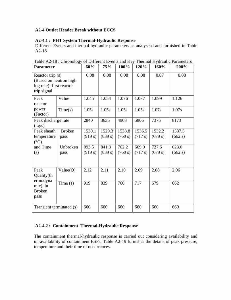
A2-4 Outlet Header Break without ECCS A2-4.1 : PHT System Thermal-Hydraulic Response Different Events and thermal-hydraulic parameters as analysesd and furnished in Table A2-18 Table A2-18 : Chronology of Different Events and Key Thermal Hydraulic Parameters Parameter 60% 75% 100% 120% 160% 200%


0.08 0.08 0.08 0.08 0.07 0.08

Peak reactor power (Factor)

Value 1.045 1.054 1.076 1.087 1.099

1.126

Time(s) 1.05s 1.05s 1.05s 1.05s 1.07s 1.07s

Peak discharge rate (kg/s)

2840 3635 4903 5806 7375 8173

Peak sheath temperature (°C) and Time (s)

Broken pass

1530.1 (919 s)

1529.3 (839 s)

1533.8 (760 s)

1536.5 (717 s)

1532.2 (679 s)

1537.5 (662 s)

Unbroken pass

893.5 (919 s)

841.3 (839 s)

762.2 (760 s)

669.0 (717 s)

727.6 (679 s)

623.0 (662 s)

Peak Quality(thermodynamic) in Broken pass

Value(Q) 2.12 2.11 2.10 2.09 2.08 2.06

Time (s) 919 839 760 717 679 662

Transient terminated (s) 660 660 660 660 660 660

A2-4.2 : Containment Thermal-Hydraulic Response The containment thermal-hydraulic response is carried out considering availability and un-availability of containment ESFs. Table A2-19 furnishes the details of peak pressure, temperature and their time of occurrences.

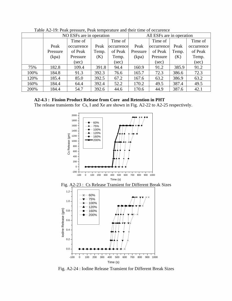
Table A2-19: Peak pressure, Peak temperature and their time of occurence NO ESFs are in operation All ESFs are in operation

Peak

Pressure (kpa)

Time of occurrence

of Peak Pressure

(sec)

Peak Temp.

(K)

Time of occurrence

of Peak Temp. (sec)

Peak Pressure

(kpa)

Time of occurrence

of Peak Pressure

(sec)

Peak Temp.

(K)

Time of occurrence

of Peak Temp. (sec)

75% 182.8 109.4 391.8 94.4 160.9 91.2 385.9 91.2 100% 184.8 91.3 392.3 76.6 165.7 72.3 386.6 72.3 120% 185.4 85.0 392.5 67.2 167.6 63.2 386.9 63.2 160% 184.4 64.4 392.4 52.2 170.2 49.5 387.4 49.5 200% 184.4 54.7 392.6 44.6 170.6 44.9 387.6 42.1

A2-4.3 : Fission Product Release from Core and Retention in PHT The release transients for Cs, I and Xe are shown in Fig. A2-22 to A2-25 respectively.

Fig. A2-23 : Cs Release Transient for Different Break Sizes

Fig. A2-24 : Iodine Release Transient for Different Break Sizes

-100 0 100 200 300 400 500 600 700 800 900 1000-200

0

200

400

600

800

1000

1200

1400

1600

1800

2000

Cs

Rel

ease

(gm

)

Time (s)

60% 75% 100% 120% 160% 200%

-100 0 100 200 300 400 500 600 700 800 900 1000

0.0

0.2

0.4

0.6

0.8

1.0

1.2

Iodi

ne R

elea

se (g

m)

Time (s)

60% 75% 100% 120% 160% 200%

Fig. A2-25 : Xe Release Transient for Different Break Sizes For most of the species 95%-98% retention has been observed in PHT system. A2-4.4 : Fission Product Behavior in Containment and Atmospheric Release Table A2-20 shows the cumulative radioactive species and related activity released into the containment after retention in PHT system Table A2-20: Cumulative activity released into the containment with PHT Retention

Break size

Iodine Krypton Xenon Cesium

(kg) (Bq) (kg) (Bq) (kg) (Bq) (kg) (Bq)

75% 6.6E-05 3.15E+14 2.4E-04 3.50E+12 4.3E-05 3.03E+14 0.11772 3.91E+14

100% 1.2E-07 5.65E+11 5.5E-05 8.23E+11 1.0E-05 7.12E+13 9.2E-05 3.05E+11

120% 4.1E-07 1.93E+12 1.0E-04 1.49E+12 1.8E-05 1.29E+14 7.7E-04 2.56E+12

160% 1.8E-08 8.33E+10 5.1E-05 7.59E+11 9.4E-06 6.56E+13 5.8E-06 1.94E+10

200% 2.3E-06 1.10E+13 2.2E-04 3.34E+12 4.1E-05 2.88E+14 6.2E-03 2.07E+13

-100 0 100 200 300 400 500 600 700 800 900 1000

0.00

0.01

0.02

0.03

0.04

0.05

Xen

on R

elea

se (g

m)

Time (s)

60% 75% 100% 120% 160% 200%

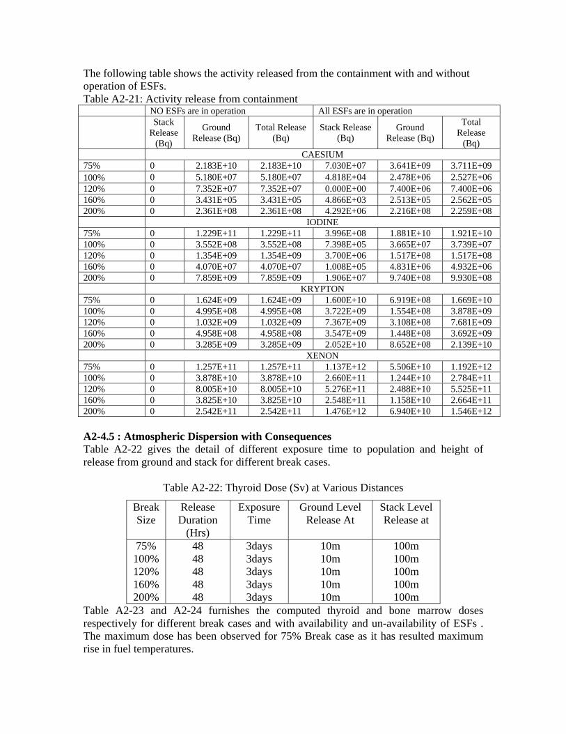
The following table shows the activity released from the containment with and without operation of ESFs. Table A2-21: Activity release from containment NO ESFs are in operation All ESFs are in operation Stack

Release (Bq)

Ground Release (Bq)

Total Release (Bq)

Stack Release (Bq)

Ground Release (Bq)

Total Release

(Bq) CAESIUM 75% 0 2.183E+10 2.183E+10 7.030E+07 3.641E+09 3.711E+09 100% 0 5.180E+07 5.180E+07 4.818E+04 2.478E+06 2.527E+06 120% 0 7.352E+07 7.352E+07 0.000E+00 7.400E+06 7.400E+06 160% 0 3.431E+05 3.431E+05 4.866E+03 2.513E+05 2.562E+05 200% 0 2.361E+08 2.361E+08 4.292E+06 2.216E+08 2.259E+08 IODINE 75% 0 1.229E+11 1.229E+11 3.996E+08 1.881E+10 1.921E+10 100% 0 3.552E+08 3.552E+08 7.398E+05 3.665E+07 3.739E+07 120% 0 1.354E+09 1.354E+09 3.700E+06 1.517E+08 1.517E+08 160% 0 4.070E+07 4.070E+07 1.008E+05 4.831E+06 4.932E+06 200% 0 7.859E+09 7.859E+09 1.906E+07 9.740E+08 9.930E+08 KRYPTON 75% 0 1.624E+09 1.624E+09 1.600E+10 6.919E+08 1.669E+10 100% 0 4.995E+08 4.995E+08 3.722E+09 1.554E+08 3.878E+09 120% 0 1.032E+09 1.032E+09 7.367E+09 3.108E+08 7.681E+09 160% 0 4.958E+08 4.958E+08 3.547E+09 1.448E+08 3.692E+09 200% 0 3.285E+09 3.285E+09 2.052E+10 8.652E+08 2.139E+10 XENON 75% 0 1.257E+11 1.257E+11 1.137E+12 5.506E+10 1.192E+12 100% 0 3.878E+10 3.878E+10 2.660E+11 1.244E+10 2.784E+11 120% 0 8.005E+10 8.005E+10 5.276E+11 2.488E+10 5.525E+11 160% 0 3.825E+10 3.825E+10 2.548E+11 1.158E+10 2.664E+11 200% 0 2.542E+11 2.542E+11 1.476E+12 6.940E+10 1.546E+12 A2-4.5 : Atmospheric Dispersion with Consequences Table A2-22 gives the detail of different exposure time to population and height of release from ground and stack for different break cases.

Table A2-22: Thyroid Dose (Sv) at Various Distances

Break Size

Release Duration

(Hrs)

Exposure Time

Ground Level Release At

Stack Level Release at

75% 100% 120% 160% 200%

48 48 48 48 48

3days 3days 3days 3days 3days

10m 10m 10m 10m 10m

100m 100m 100m 100m 100m

Table A2-23 and A2-24 furnishes the computed thyroid and bone marrow doses respectively for different break cases and with availability and un-availability of ESFs . The maximum dose has been observed for 75% Break case as it has resulted maximum rise in fuel temperatures.

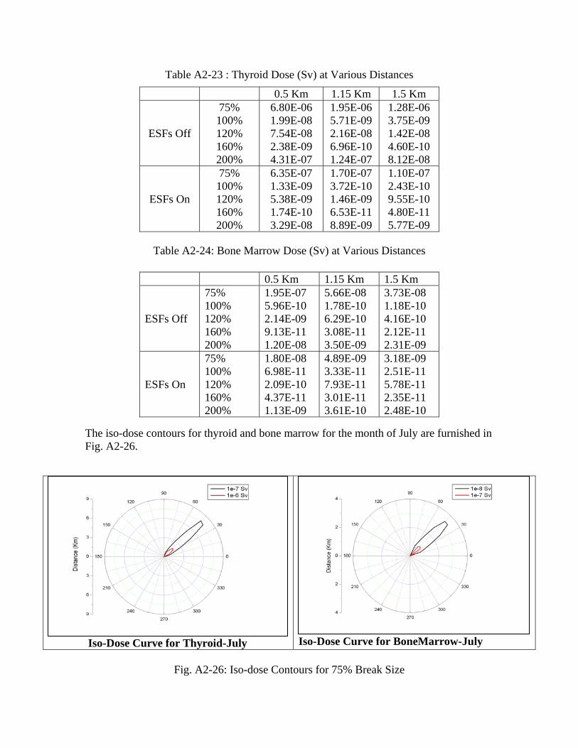
Table A2-23 : Thyroid Dose (Sv) at Various Distances

Table A2-24: Bone Marrow Dose (Sv) at Various Distances

The iso-dose contours for thyroid and bone marrow for the month of July are furnished in Fig. A2-26.

Fig. A2-26: Iso-dose Contours for 75% Break Size

0.5 Km 1.15 Km 1.5 Km

ESFs Off

75% 100% 120% 160% 200%

6.80E-06 1.99E-08 7.54E-08 2.38E-09 4.31E-07

1.95E-06 5.71E-09 2.16E-08 6.96E-10 1.24E-07

1.28E-06 3.75E-09 1.42E-08 4.60E-10 8.12E-08

ESFs On

75% 100% 120% 160% 200%

6.35E-07 1.33E-09 5.38E-09 1.74E-10 3.29E-08

1.70E-07 3.72E-10 1.46E-09 6.53E-11 8.89E-09

1.10E-07 2.43E-10 9.55E-10 4.80E-11 5.77E-09

0.5 Km 1.15 Km 1.5 Km ESFs Off

75% 100% 120% 160% 200%

1.95E-07 5.96E-10 2.14E-09 9.13E-11 1.20E-08

5.66E-08 1.78E-10 6.29E-10 3.08E-11 3.50E-09

3.73E-08 1.18E-10 4.16E-10 2.12E-11 2.31E-09

ESFs On

75% 100% 120% 160% 200%

1.80E-08 6.98E-11 2.09E-10 4.37E-11 1.13E-09

4.89E-09 3.33E-11 7.93E-11 3.01E-11 3.61E-10

3.18E-09 2.51E-11 5.78E-11 2.35E-11 2.48E-10

Iso-Dose Curve for Thyroid-July Iso-Dose Curve for BoneMarrow-July

barc/2009/e/013 government of india atomic

Documents