Anderson Localization, Non-linearityand

Stable Genetic Diversity

Charles L. Epstein∗

Department of Mathematicsand

Laboratory for Structural NMR ImagingUniversity of Pennsylvania

February 28, 2006

Abstract

In many models of genotypic evolution, the vector of genotype populations satis-fies a system of linear ordinary differential equations. This system of equations mod-els a competition between differential replication rates (fitness) and mutation. Muta-tion operates as a generalized diffusion process on genotype space. In the large timeasymptotics, the replication term tends to produce a single dominant quasispecies,unless the mutation rate is too high, in which case the populations of different geno-types becomes de-localized. We introduce a more macroscopic picture of genotypicevolution wherein a random replication term in the linear model displays featuresanalogous to Anderson localization. When coupled with non-linearities that limit thepopulation of any given genotype, we obtain a model whose large time asymptoticsdisplay stable genotypic diversity.

IntroductionThis paper contains a proposal for a class of theories of genotypic evolutionthat display stable, arbitrarily complex genetic diversity. Our models are builtout of pieces that have been on the shelves for quite a while, but perhaps havenot before been placed together.

∗Research partially supported by DARPA under the FUNBIO program.Keywords: quasispecies, spin glass models, non-linearity, Anderson localization, genotypic diversity,paramuse model, Eigen model.

1

We start out with linear “spin glass” models, which cast genotypic evolu-tion as competing processes of replication and mutation. We posit the exis-tence of sequences, {Rn}, of replication (or fitness) matrices so that the com-bined replication-mutation system exhibits properties, in the thermodynamiclimit of large genome length, analogous to Anderson localization. Such amodel already exhibits a weak form of genetic diversity, having a large num-ber of well defined, well separated, “long-lived” quasi-species. In a linearmodel it is more or less inevitable that, in the long run, either a single speciescomes to dominate, or localization breaks down and there are no well de-fined quasispecies. Our additional step is to add a quadratic term that limitsthe growth of any given genotype. This step is suggested by a paper of Nel-son and Shnerb, where they show, in a continuum population biology model,that such a term, when coupled to Anderson localization does in fact lead toan asymptotic state with stable diversity, see [8].

The main contribution of this paper is to put these two pieces togetherin the context of genotypic evolution and suggest potentially fruitful direc-tions for further research in both evolution and spectral theory. In small nu-merical examples we show that our localization hypothesis is not unreason-able. The rigorously established results showing that localization occurs forSchrodinger operators with sufficiently weak diffusion, and that, when it oc-curs, is generic, gives support for the idea that such models should exist andthat the localization property should be insensitive to the details of the model.Finally, there is a certain sublime beauty to a world in which the randomnessof the mapping from genotype to fitness conspires with environmental limi-tations on population size to produce stable genetic diversity.

AcknowledgmentsI would like to thank Ben Mann for insisting that I participate in the FUNBIO

program and securing the funding to make it happen. I am very thankful to all par-ticipants in the DARPA FUNBIO workshops and most especially to Richard Lenski,Sally Otto, Michael Deem, Jeong-Man Park, Chris Adami, and Jack Morava for shar-ing their ideas on biology and evolution with me. I would also like to thank MichaelDeem for several useful suggestions for improvement of an earlier drafts. Finally Iam very grateful to Harvey Rubin for telling me the biochemical facts of life and toJohn Schotland for his considerable help with statistical mechanics and many usefulsuggestions related to this work.

1 Linear modelsRecently there has been a great deal of interest in the connections betweenvarious models that arise in statistical mechanics and models of genetic evo-lution. Early models were defined by Eigen and Crow-Kimura, see [5, 4]. Fora good survey of this subject with many references to the literature see [7].Genotypes are described as sequences (s1, . . . , sn),where the entries {s j } aredrawn from a finite alphabet. For example, if one wishes to model chromoso-

2

mal evolution the alphabet is that of nucleotides {A,C,G, T } (or, for RNA,{A,C,G,U}). If one wishes to studies protein evolution, then one mightuse the list of the 20 amino acids. In the interest of simplicity, most investi-gators simply use a two letter alphabet, which can be thought of as purinesand pyrimidines. We let Gn,l denote the set of possible genotypes of lengthn expressed in the given fixed alphabet with l members. If all genotypes arepossible, then |Gn,l| = ln . In the sequel we let N = ln . The different geno-types can therefore be labeled by the set of integers Jn,l = {1, 2, . . . , N},though this labeling scheme conveys no further information.

We specify a model for mutation from one genotype to another by as-signing probabilities {m i j : i 6= j ∈ Jn,l} that, in a given unit of time, thegenotype Si mutates to the genotype S j . If we think of Gn,l as the vertices ofa directed graph, then we add a directed edge from Si to S j if mi j > 0. LetP(t) = (P1(t), . . . , PN (t)), where Pj (t) is the population of the genotypeS j at time t . In addition to mutation, each genotype has a replication rate,ri so that, in the absence of mutation we would have the simple differentialequation describing the change of the population of genotype S j . :

d Pi

dt= ri Pi (t). (1)

Hence ri is the difference of the birth and death rates for the genotype Si .

The replication matrix, R, is defined to be

Ri j =

{

0 if i 6= jri if i = j.

(2)

This matrix is often called the “fitness” matrix, but following a suggestion ofMichael Deem, we use the more precise term “replication” matrix.

The mutational process is described by the mutation matrix, M, givenby:

Mi j ={

m j i if i 6= j−

∑

k 6=i mik if i = j.(3)

The negative diagonal term is required so that the total mutational flux outof a given genotype, is balanced by an equal decrease in its population. Thestandard linear model for the time course of the genotype populations is then

d Pdt

= R P + M P . (4)

In many prior papers on this subject, the model is described as a model forpopulation densities, rather than the populations themselves. These modelsare equivalent, under a simple change of variables, to a linear model, andit is the linear model that is amenable to analysis. For many choices of Rand M, these models have convenient representations in terms of Pauli spin

3

matrices, which in turn allows the application of techniques developed tostudy spin glass models in statistical mechanics.

In most of the previous analyses of these models, the alphabet has 2 let-ters. If Si = (s1, . . . , sn), S j = (s ′

1, . . . , s′n) are two genotypes, then the

Hamming distance between them equals the number of entries where theydiffer. If we represent the genotypes as sequences of plus and minus ones,then

dH (Si , S j ) =12

[

n −n

∑

k=1

sks′k

]

. (5)

If our alphabet has l-letters, then more generally we can define a metric byfirst defining a metric on the alphabet: let A = {a1, . . . , al} then dA : A ×A → [0,∞) is a function that satisfies:

dA(ai , a j ) ≥ 0 and equals 0 only if i = j.

dA(ai , a j ) = dA(a j , ai) for all pairs i, j.

dA(ai , a j ) ≤ dA(ai , ak)+ dA(ak, a j ) for all triples i, j, k.(6)

The Hamming metric on Gn,l is then defined by

dH,A(Si , S j ) =n

∑

k=1

dA(sk , s′k). (7)

In earlier papers, which consider an alphabet with two letters, the muta-tion probabilities are often taken to be functions of the Hamming distance.In the paramuse model the mutation matrix is specified by

Mi j =

µ if dH (i, j) = 1−nµ if i = j0 otherwise.

(8)

The probability-per-unit-time of changing one letter is µ and the probabilityof changing more than one letter is zero. In the Eigen model, m i j is a functionof the Hamming distance between i, j of the form

mi j = µdH (Si ,S j )(1 − µ)n−dH (Si ,S j ). (9)

The assumption here is that probability-per-unit-time of mutation at each siteon the genome is equal to that of every other, and that they are also indepen-dent of one another. In this case the division between mutation and replica-tion is not as simple. In our subsequent analysis we stick to the representationgiven in (4). The precise nature of M is less important than the assumptionthat the semi-group et M should have the qualitative properties of a diffusionprocess:

1. It should be positivity improving, i.e. if P0 is a vector with non-negative coefficients, then et M P0 has positive coefficients.

4

2. It should decay very rapidly as we depart from the diagonal.

These conditions amount to the requirements that the off-diagonal entries ofM are non-negative and rapidly decaying as we depart from the diagonal.

The population vector P defines a function on the vertices of the geno-type graph Gn,l . In these models, a quasi-species is represented by a popula-tion vector that is highly concentrated around a single vertex or small clusterof vertices. A population vector with several such clusters, which are wellseparated on the graph, would represent a collection of quasi-species. Themutational process is a diffusion on this graph. The eigenvectors of the ma-trix M are not localized. The Perron-Frobenius Theorem implies that thelargest eigenvalue of M, λP, corresponds to an eigenvector vP all of whoseentries are positive. Indeed, usually vP = (1, . . . , 1). Under the effects ofmutation alone, any initially non-negative population, P0, behaves asymp-totically as

P(t) ∼ 〈P0, vP 〉vPeλP t . (10)

So the effect of the mutational process is to smear out the population and de-stroy any localized populations that might be present in the initial distributionof genotypes.

On the other hand, the replication matrix R is diagonal and if it has dis-tinct entries, then each basis vector e j = (0, . . . , 0, 1, 0, . . . , 0) (1 in the j thplace) defines a quasi-species. In the absence of mutation, the population ofthis quasi-species evolves as er j t Pj (0). Indeed the matrices {et(R+M) : t >0} are also positivity improving and hence have a positive Perron-Frobeniuseigenvector, vP, corresponding to the largest eigenvalue, λP . From our per-spective, the problem here is that, in the long time limit, the population willagain satisfy (10) and be dominated by the population distribution (quasi-species or not) with this highest replication rate. For most of the analysesof these models this was not really viewed a difficulty, as the problem underanalysis was the stability of a single quasi-species under various levels ofmutation, and for various choices of smooth replication landscape.

By smooth we mean that the replication rate is smooth as function of thegenotype with respect to the distance function defined on Gn,l . This sort ofanalysis can be regarded as focusing on a small neighborhood of a vertex inGn,l . If we assume that m << n sites participate in the evolutionary process,then the analysis proceeds on Gm,l viewed as a subgraph of Gn,l . On this sub-graph (length scale), even a macroscopically random replication landscapecould well appear quite smooth. Hence, thermodynamic analyses, like thatin [11], can be viewed as genotypically localized, short time analyses thattake place within the larger macroscopic framework of genetic evolution.

In this paper we consider questions related to the long time macroscopicstructure of genotypic evolution. We focus on aspects of linear models thatare connected to the randomness of the replication rate matrix, and beyondthat on the consequences of non-linear corrections that are needed to accountfor the finiteness of resources. Our ideas related to randomness and localiza-

5

tion are inspired by the seminal work of P.W. Anderson [2], and the effectsof non-linear corrections, by the work of D.R. Nelson and N.M. Shnerb inpopulation biology, see [8].

2 Anderson LocalizationThe combined linear model given in (4) represents a competition betweenthe replication term, which, if the diagonal entries are random, tends to pre-serve quasi-species, and the mutation term, which tends to destroy them. Assuch, these models have a great deal in common with the models for conduc-tion in semiconductors studied by Anderson. In his seminal work and manysubsequent analyses, it has become clear that there is a very fundamentaland generic localization property shared by systems with a random “poten-tial.” Before proceeding with out discussion, we briefly discuss the analysisof continuum models of the form:

ut(x, t) = (L + E)u(x, t) whereLu(x, t) = µ1u(x, t)+ q(x)u(x, t),

(11)

with x ∈ Rp, t ∈ [0,∞), and E a positive constant. It is well known

that these equations are positivity improving: if u(x, 0) ≥ 0 for all x, thenu(x, t) > 0 for all x and t > 0, see [10]. We are therefore free to interpretu(x, t) as the density of the population located at position x at time t .

While it is very difficult to see how an evolutionary model, with underly-ing space a graph like Gn,l, can be approximated by a continuum model likethat in equation (11), there are strong structural analogies between this typeof evolution equation and (4). Under time evolution, the first term, µ1u,generates a spatially homogeneous diffusion process. As time goes to infin-ity, this term will lead to a spatially uniform population. The multiplicationoperator q(x) is analogous to the replication matrix. We include E to have abackground environmental energy or temperature in the problem.

Formally, the solution to (11) is given by

u(x, t) = et Eet Lu(x, 0). (12)

The qualitative behavior of the solution is determined by the spectral theoryof L . There are three simple possibilities (and many cases where the answeris not known). If q decays, sufficiently rapidly, as ‖x‖ tends to infinity, thenusually the spectrum of L consists of purely absolutely continuous spectrumin (−∞, 0], along with some L2-eigenstates with positive eigenvalues. Thereare, at most, finitely many L2-eigenstates with eigenvalues in an interval ofthe form [ε,M], where ε > 0, though the positive spectrum can accumulateat 0. If there are no L2-eigenstates then a localized initial condition spreadsout as t → ∞. If there are L2–eigenstates, then the corresponding eigen-vectors usually have large overlaps in their supports. If there is a maximum

6

positive eigenvalue λ0, with a positive eigenvector, ψ0, (a vacuum state),then asymptotically the solution behaves like 〈ψ0, u(·, 0)〉ψ0e(E+λ0)t .

Another simple possibility is that q(x) tends to infinity as ‖x‖ tends toinfinity. In this case the spectrum is pure point spectrum,

{λ0 > λ1 ≥ λ2 ≥ . . . },

with each eigenvalue of finite multiplicity, and lim j→∞ λ j = −∞. Let {ψ j }be the eigenstates. These are localized functions, but typically their sup-ports have considerable overlap. An important special case is given by theq(x) = ‖x‖2, the harmonic oscillator. The eigenfunctions are of the formp j(x)e− 1

2 ‖x‖2, where p j(x) are polynomials. In the large time limit, the

solution again behaves like 〈ψ0, u(·, 0)〉ψ0e(E+λ0)t . Since q is unbounded,this case would not appear to have much to do with the evolutionary modelsabove. These two cases are extensively described in [10].

The third case is that q remains bounded but has no asymptotic or peri-odic behavior as ‖x‖ → ∞. These are what are often referred to as “randompotentials” in the mathematics literature. A simple example would be an al-most periodic function like cos x + cos

√2x . In this case the spectrum of L

can behave in a very remarkable way. In his seminal 1958 paper, [2, 13],Anderson argued that, when µ is not too large, the operator L has densepoint spectrum lying in intervals, and the corresponding eigenfunction areexponentially localized. Though it required the development of consider-able analytic technique, the substance of these assertions has been verified inmany special cases. In one and two dimensions (i.e. x ∈ R or R

2) it has beenshown that, with probability one (with respect to the choice of potential), thespectrum of L is dense pure point spectrum on a half line {λ j } ⊂ (−∞, λ0]and the corresponding eigenfunctions {ψ j } fall off exponentially. That is, theclosure of the set {λ j } is the half line (−∞, 30], and

Lψ j = λ jψ j

|ψ j (x)| ≤ C j e−|x−x j |ξ j .

(13)

In higher dimensions, more complicated things can happen. For example,one could have dense point spectrum in an interval [31, 30], and then aninterval of continuous spectrum [33, 32]. Nonetheless the appearance of in-tervals of dense point spectrum is a generic property for many classes ofpotentials. Discrete models, analogous to (11), defined for functions on thelattices have also been extensively studied. For sufficiently weak diffusion,Anderson localization has also been shown to be a generic property. See[6, 9, 3] for mathematical results in this field and further references.

The third case seems to be closest to what is expected of a realistic repli-cation landscape: the replication rate is constantly varying throughout geno-type space and is neither periodic nor has any asymptotic behavior. This doesnot preclude the replication landscape from being locally smooth or having

7

large regions where it is approximately constant. We let {Ln = Rn + Mn}denote a sequence of operators acting on functions on Gn,l . In our subsequentanalysis we use the following localization ansatz:

As n tends to infinity, the spectrum of the operators Ln becomesdense in some interval with right end point sup spec(Ln). Thecorresponding normalized eigenvectors become exponentiallylocalized, with the overlaps in support uncorrelated to the dif-ferences in energy.

One might want to suppose that the matrices {Rn} converge to a infinite diag-onal matrix R∞ and the sequence of discrete diffusion operators {Mn} con-verge, in some sense, to an operator acting on `2. It is by no means obvioushow to normalize the sequence {Mn} so that the limit produces a non-trivialdiffusion process. At realistic mutation rates, genotype space seems to be ex-plored very slowly, so there is not much practical difference between a verylarge, but finite length genome, and an infinite length genome.

In the random case, the degree of overlap of eigenvectors should not becorrelated to the difference in energies, i.e. if λi and λ j are nearby eigenval-ues it is highly unlikely that the supports of the corresponding eigenvectorsψi and ψ j have a substantial overlap. If the diagonal matrix Rn has distinctand say strictly monotonically increasing entries, then it is again the casethat, for small enough µ, the eigenvectors of Ln are highly localized. Whatdistinguishes this case from the random case is that now the overlap in theeigenvectors is highly correlated with the difference in energy: if |λi − λ j | issmall then is very likely that the supports of ψi and ψ j have a large overlap.This becomes quite important when we consider the effects of the non-linearcorrections.

To the best of my knowledge, this precise situation has not yet been an-alyzed, though considerable effort has been devoted to studying analogousquestions on the lattices Z

d, and Anderson localization has been rigorouslyestablished in many representative cases, see [9]. In the physics literature ithas been shown that Anderson Localization occurs for a system based on theBethe lattice, see [1]. This is of interest for us, as the Bethe lattice embedsisometrically into the hyperbolic plane. Hence this indicates that the moreefficient diffusion that occurs in negatively curved spaces does not destroyAnderson Localization. In the final section we give some numerical exam-ples suggesting that this sort of localization does occur on the graphs Gn,l .

Anderson localization is a phenomenon that exhibits phase transitions:for sufficiently small diffusion or at sufficiently low energies it can be ex-pected to occur, but as the diffusion rate or energy become too large it mayabruptly disappear, with the pure point spectrum being replaced by continu-ous spectrum. Such a transition would have interesting consequences for theunderlying genetic system.

8

Remark 1. There is a somewhat different infinite n limit of genotype spacethat may be more appropriate than simply taking the genome length to infin-ity. We could also consider the space

Gs∞,l =

∞⊔

n=1

Gn,l . (14)

The space Gs∞,l contains genotypes of all different lengths, and provides a

framework for studying interactions, i.e. recombination and splicing, amongthe genetic material of very different types of organisms, e.g. viruses andeukaryotes. It would seem an important question to understand under whatmutational structures, generic random replication landscapes exhibit local-ization on Gs

∞,l . It may also provide a framework where it is easier to takethe thermodynamic limit of the mutation process.

3 Weak genetic diversityBefore considering the role of non-linearities, we consider what a linearmodel satisfying the localization ansatz would predict. Let us fix a large valueof n so that Ln has many exponentially localized, well separated eigenstatesnear the supremum of the spectrum. Indeed we normalize so that

sup spec(Ln) = 0. (15)

We follow the continuum model and explicitly include an energy, whichcould represent an environmental temperature, in our system:

d Pdt

= (Ln + E)P . (16)

In a linear model the addition of E has no qualititative effect on the solution,it simply scales the result by et E . As we shall see, this is no longer the caseonce we include non-linear corrections.

The localization ansatz is that, near to 0, there is a large number of eigen-values {0 = λ0 ≥ λ1 ≥ . . . }, such that the corresponding normalized eigen-vectors {ψα} are highly localized, and the overlaps in their supports are un-correlated with their energy differences. Quantitatively we take this to meanthat for each α, there is a jα ∈ Gn,l and positive numbers ξα,Cα, so that

ψα( j) < Cαe− dH ( j, jα)ξα , (17)

and for α 6= β∑

j∈Gn,l

|ψα( j)ψβ( j)| << 1, (18)

9

with high probability, especially if |λα − λβ | is small. Moreover, we assumethat {ψα( j)} is positive for most values of j. Because of exponential local-ization, this assumption does not contradict the fact that the eigenvectors arean orthonormal set.

If P0 is an initial population distribution, then evolving under equa-tion (16), the population satisfies:

P(t) =∑

α

〈P0, ψα〉ψαe(E+λα)t . (19)

For long times only the terms with E + λα > 0 make a significant contribu-tion to P(t). The λ0-term is still the dominant term, but there may be manyterms with λ0 − λα quite small, which therefore make significant contribu-tions for a long time. Because the eigenstates are well localized and wellseparated, there can well be different dominant terms at different locationsin genotype space. Thus, even without non-linear corrections, a model sat-isfying the localization ansatz would exhibit some sort of genetic diversity,which we call weak genetic diversity.

4 Non-linear effectsNelson and Shnerb modify the model in (11) by adding a non-linear term:

ut(x, t) = (L + E)u(x, t)− bu2(x, t), (20)

where b > 0. The effect of this term is to limit u(x, t) to remain less thanE/b. More generally if b is replaced by any positive L + E-super-harmonicfunction, B(x), so that, for all x,

(L + E)B(x)− B3(x) < 0, (21)

then the maximum principle shows that if initial data u(x, 0) < B(x) for allx, then u(x, t) < B(x) for all x and t > 0.

The remarkable observation made by Nelson and Shnerb is that, if Lexhibits Anderson localization, then the large time asymptotics of the non-linear equation actually depend on all the eigenvalues of L with λα + E > 0.If we let

cα(t) = 〈u(·, t), ψα 〉, (22)

then, under (20), they evolve according to:

cα(t)dt

' (E + λα)cα(t)−wαc2α(t), (23)

wherewα = b

∫

ψ3α(x)dx . (24)

10

Because the eigenstates are highly localized, the coefficients for the crossterms

b∫

ψα(x)ψβ(x)ψγ (x)dx (25)

are very small, and that is why they can be ignored. We can solve (23) toobtain:

cα(t) =cα(0)e(E+λα)t

1 + cα(0) wαE+λα (e

(E+λα)t − 1). (26)

Hence as t → ∞, all species such that E + λα > 0 and cα(0) > 0 have afinite, non-zero asymptotic value given by

limt→∞

cα(t) =E + λα

wα. (27)

Here we see the importance of the “E-term” in a non-linear model.We can apply similar considerations to a somewhat larger class of mod-

els, in which we include a second non-linearity to limit the total population

ut(x, t) = (L + E)u(x, t)− B(x)u2(x, t)− pu(x, t)∫

u(x, t)dx . (28)

The second, non-local term, can be shown to impose a limit on the totalpopulation

∫

u(x, t)dx, which the first term does not do. One can also showthat, so long as B(x) > c > 0, the asymptotic behavior of a non-negativesolution of (28) is similar to that for (20). If B ≡ 0, then the model in (28)has many critical points, none stable and none with a large number of non-zero coefficients.

The analogue of the model in (20) is an equation of the form:

d P(t)dt

= (L + E)P(t)− b P(t). ∗ P(t). (29)

Here we use the MATLAB notation for component-wise vector multiplica-tion: if v = (v1, . . . , vm) and w = (w1, . . . , wm), then

v. ∗ w = (v1w1, v2w2, . . . , vmwm). (30)

For this discussion we take M given by (3), though much of what we sayshould remain true with any reasonable choice of M. Let B be a positivesuper-harmonic vector (L + E)B − B. ∗ B. ∗ B < 0. If we replace (29) with

d P(t)dt

= (L + E)P(t)− B. ∗ P(t). ∗ P(t), (31)

and 0 ≤ Pj (0) < B j for all j, then 0 ≤ Pj (t) < B j for all j and t > 0. Amodel similar to (28) is given by

d P(t)dt

= (L + E)P(t)− B. ∗ P(t). ∗ P(t)− p〈P, 1〉P, (32)

11

where p > 0 and 1 = (1, . . . , 1). These models are all positivity preserving.Their basic mathematical properties are established in the Appendix. Forsimplicity we proceed with the model given in (29).

As noted, the solution operator for equation (29) is positivity preserving.If

c =sup{E + r j }

b, (33)

then a simple maximum principle argument shows that, if 0 ≤ P j (0) < c, forall j, then 0 < Pj (t) < c for all t > 0. If L satisfies the localization ansatz,then the analysis used to derive (23)–(27) applies, mutatis mutandis to (29).The spectrum, {λα}, of L is quite dense near to zero, and the correspondingeigenvectors, {ψα} are highly localized. As before we express the initial dataas

P(0) =∑

α

〈P(0), ψα〉ψα =∑

α

cα(0)ψα. (34)

We need to express the non-linear term in the eigenbasis:

wαβ,γ = 〈B. ∗ P(t). ∗ P(t), ψγ 〉 = b∑

j

∑

α,β

cα(t)cβ(t)ψα( j)ψβ( j)ψγ ( j).

(35)The localization ansatz implies that in general, unless α = β = γ, wαβ,γis very small, especially if |λα − λβ | is small. We set wα = wαα,α. Hence,the coefficients again satisfy (23) and therefore the solution is again givenby (26), with long time asymptotics given by (27),

limt→∞

cα(t) =E + λα

wα. (36)

Thus we see that coupling localization in genotype space with a simple non-linearity produces a model exhibiting long time genetic diversity. We get alarge collection of distinct quasi-species occupying different parts of geno-type space.

What distinguishes a random replication matrix from one with mono-tonely increasing diagonal entries is that, in the latter case, the eigenvec-tors with large overlaps in their supports tend to have nearby energies. Thismeans that, when the non-linear terms are included, paths exist in the energylandscape defined by the spectral theory of L that give the population the op-portunity to cascade toward states with lower energy. This claim is born outby the numerical simulations of the non-linear equation in the next section.In the random case no such paths exist and this further supports our claimthat these models will display stable genetic diversity. It also suggests a con-nection between these models and an interesting percolation problem on anenergy landscape defined by the spectral theory of L .

There are a variety of other interesting phenomena that could be obtainedwith models satisfying the localization ansatz. For example, if L has a band,

12

lying below the localized states, of eigenvalues with non-localized eigen-states, then an increase in E to E ′, would require re-expressing the data interms of the new eigenstates with λα + E ′ > 0, which would include somestates with non-localized eigenvectors. Evolution at this higher energy couldresult in significant shuffling of the genotype populations. If the energy sub-sequently dropped back to a range where the relevant eigenstates are againlocalized, then the system would eventually settle into a steady state withconsiderable genetic diversity, possibly quite different from the state we hadprior to the temporary increase in energy.

5 Numerical examplesIn this section we present some numerical evidence for the localization ansatz.In a variety of papers, notably in [11], it is shown that, in order for quasi-species to exist in the large n limit, it is necessary that nµ be less than themaximal diagonal term in the replication matrix. For our numerical simula-tions we divide by n so that µ is fixed and

Mi j =

−µ if i = jµn if dH (i, j) = 10 otherwise.

(37)

We then compute the eigenvalues and eigenvectors of matrices of the formL = R + M, where R is a diagonal matrix with (pseudo)random, uni-formly distributed entries, scaled to lie in [0, 1]. Physically this amountsto replacing the time parameter t by t/n. For purposes of comparison, wealso consider diagonal matrices with distinct but smoothly growing entries,e.g. Rii = tanh(2−ni), and replication matrices arising in single peak fitnesslandscapes, Rii = 1/(1 + dH (Si , S0)). Our numerical experiments displayseveral striking phenomena.

For a given matrix L, let {λα} denote the spectrum and {ψα(k)}, the cor-responding normalized eigenvectors. The eigenvalues are indexed in increas-ing order. In our experiments we see that, with a random replication matrix,the spectrum is distributed fairly uniformly over an interval, with decreasingdensity near the upper endpoint. This is in agreement with known results onthe spectral density function in the continuum case, see [2, 13]. The matriceswe consider are symmetric, so the eigenvectors are real and orthonormal:

2n∑

k=1

ψα(k)ψβ(k) = δαβ . (38)

To measure the extent of the overlap in the support of the eigenvectors we

13

compute the following sums

Cαβ =2n∑

k=1

|ψα(k)ψβ(k)|. (39)

If the eigenvectors were perfectly localized then the matrix, Cαβ−δαβ,would

be zero. If the eigenvectors were completely de-localized, like (2− n2 e

2π i jk2n :

k = 0, . . . , 2n − 1), then Cαβ = 1 for all α, β. A more compact measure ofmean localization is provided by the averages along rows:

Cα =12n

∑

β 6=αCαβ . (40)

Figures 1–2 show the results of simulations for n = 7 and 11. The upperrow of each figure is a surface plot of log10 Cαβ (suitably cutoff from below)for a random replication matrix (on the left) and for Rii = tanh(2−ni) (onthe right). As noted above, the random model has a uniformly distributeddiagonal scaled to lie in the interval [0, 1]. We use the tanh-function, whichhas well defined asymptotics, to avoid harmonic oscillator-like behavior. Forthese examples µ = 10−5.

The lower rows of these figures are plots of log10(2−n ∑

β Cαβ). We seethat, as n grows, the models with random replication matrices tend stronglytoward localization. Moreover, the overlaps tend to be quite random and un-correlated with energy differences. If Rii = tanh(2−ni), then the eigenvec-tors also tend to be rather localized, though not as strongly as in the randomcase. However the pattern of overlap is highly correlated with the energydifference, and entirely different from the random case. In Figure 3 we showthe same data, with n = 11 and µ = 10−5, but this time using a single peakreplication matrix: Rii = 1/(1 + dH (Si , S0)), with S0 = (1, . . . , 1), as the“smooth” model. In this case the spectrum of the smooth model is highly de-generate. We again show both plots as the random model is computed with adifferent realization of R. In this case the eigenvectors of the smooth modelare highly correlated.

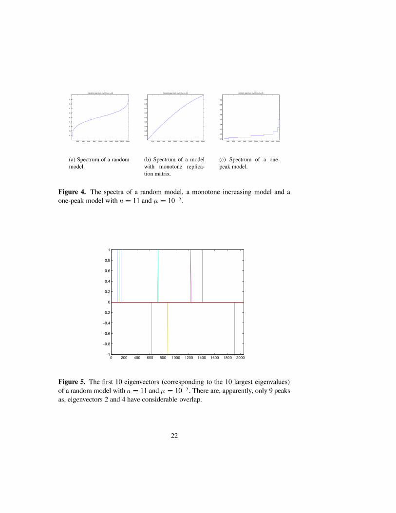
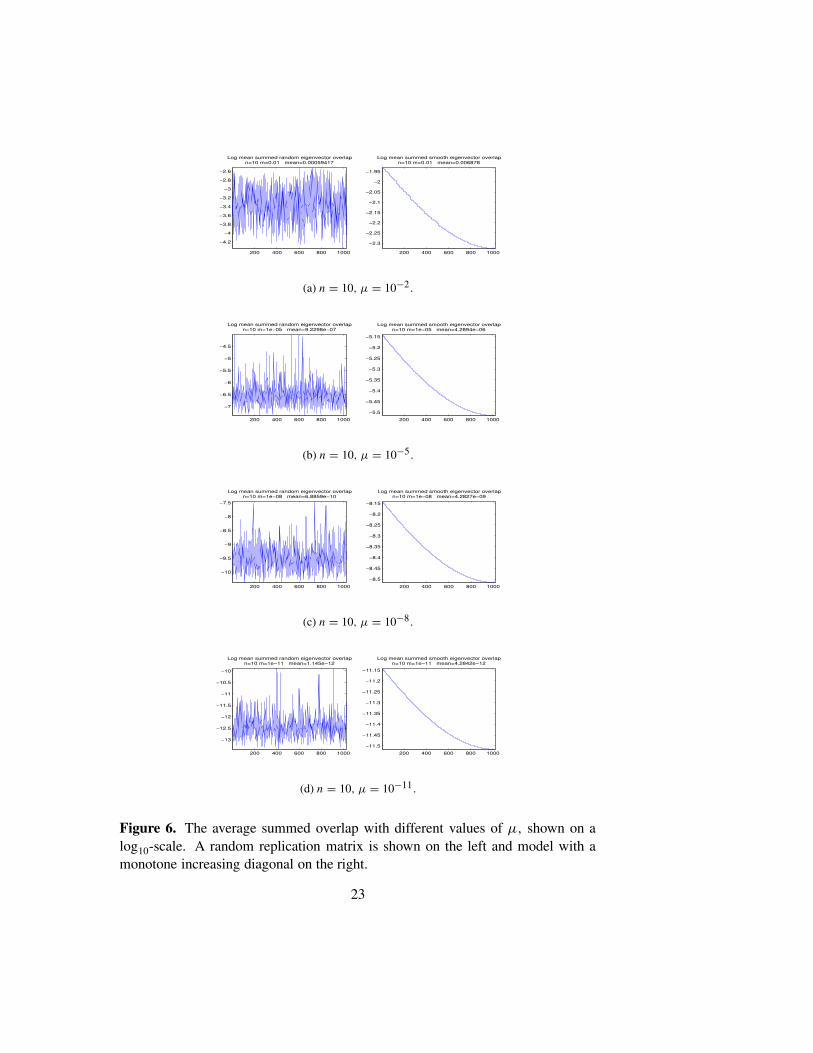
In Figure 4 we show the spectra of L for the examples considered in Fig-ures 2 and 3. For the random model, the spectrum is dense in an interval,and thins out toward the endpoints. The monotone model also has a densespectrum, whereas the one-peak model has a highly degenerate spectrum.Figure 5 shows the first ten eigenvectors of a random model with n = 11and µ = 10−5. This largely bears out our claim that the overlap in the eigen-vectors is uncorrelated with the energy difference, though, in this example,eigenvectors 2 and 4 have considerable overlap. In a similar plot (not shown)using the monotone model, all 10 eigenvectors are located at the extreme leftedge and cannot be visually distinguished. Figure 6, shows the effect on themean overlap in the eigenvalues as µ is decreased, while n is kept fixed. Wesee that the mean overlap is roughly proportional to µ. In Figures 1–2(c) we

14

see that the mean overlaps for n = 7, 9, 11 are 3 × 10−6, 1 × 10−6, 3 × 10−7

respectively, indicating that as the genome length increases the degree of lo-calization of the eigenvectors is monotone increasing.

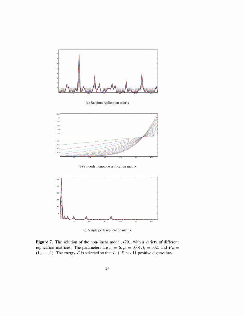
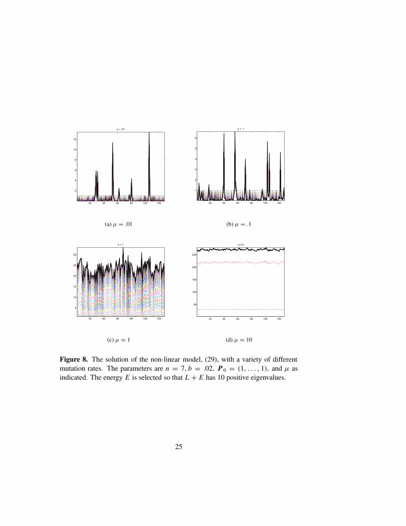
Figure 7 shows the results of solving (29) numerically, with three dif-ferent types of replication matrices. Several time steps are shown, with theasymptotic state clearly indicated as the outer envelope. As above the diag-onal entries of R are scaled to lie in [0, 1], we use n = 6, µ = .001, andb = .02.The equation is solved using Strang’s splitting method applied to thenon-linear Kato-Trotter product formula. The parameter E is selected so thatL + E has 11 positive eigenvalues. The initial data is P0 = (1, . . . , 1). Fig-ure 7(a) shows the results with a random replication matrix. There appear tobe only 10 distinct asymptotic quasispecies, though in fact the two left-mostpeaks have merged to form a plateau. The analysis presented in Section 4 isentirely born out in this numerical experiment. Figure 7(b) shows the resultswith a smooth monotone replication matrix. As predicted, the population hascascaded to form a single poorly localized quasispecies. In the final exam-ple, we use the single peak matrix, Rii = 1/(1 + dH (Si , S0)). As expected,this replication matrix produces one dominant quasispecies. Several smaller,but well localized quasispecies are also in evidence. The final set of figuresshows the phase transition that occurs as the mutation rate is increased. ForFigure 8, we solved (29) with n = 7, b = .02, and µ = .01, .1, 1, 10. Thetransition from localized populations to delocalized populations is quite ap-parent. For each figure we use a different random replication matrix.

A Mathematical AppendixWe consider models of the following general type:

d Pdt

= L P − P. ∗ P . ∗ B − β〈P, 1〉P (41)

where B is a pointwise positive super-harmonic vector andβ is a non-negativenumber. Here L = R + M, where R is a diagonal matrix and M is a matrixwith zeroes on the diagonal and non-negative entries off the diagonal.

In order for such an equation to define a reasonable population model, itis necessary that it be positivity preserving. That is, if the initial data P(0)has non-negative entries, then P(t) is non-negative for all t > 0. The modelsof the type given in (41) have this property. This is established in two stepsand uses the Kato-Trotter product formula and its non-linear generalization.

We first treat the linear part. The solution to the linear equation ∂t P =L P is given by

P(t) = et L P(0) = et(R+M)P(0), (42)

where, for a finite dimensional system, the matrix exponential is given by the

15

usual formula, e.g.

et L =∞∑

j=0

(t L) j

j !. (43)

From this expression it is immediate that et M has non-negative entries forevery t > 0. Indeed for the models considered above et M has positive en-tries for all t > 0. Because R and M do not commute, it does not followimmediately that et(R+M) also has positive entries. To prove this we use theKato-Trotter product formula, which states that

et(R+M) = limn→∞

[

etn Re

tn M

]n. (44)

As the right hand side expresses et(R+M) as a limit of products of matriceswith non-negative entries, it follows that et L also has non-negative entries.With a little more care we can show that, in fact, et L has positive entries.Hence the linear model is positivity preserving. For a thorough discussion ofpositivity preserving operators see section XII.12 of [10].

In [12] a non-linear generalization of the Kato-Trotter formula is givenfor non-linearities including the type in (41). We first observe that the vectorfield defined on R

2nby

X (P) = −P. ∗ P . ∗ B − β〈P, 1〉P (45)

is tangent to the coordinate hyperplanes {P : P j = 0}, and therefore thepositive orthant, {P : Pj > 0 for all j}, is invariant under the flow generatedby this vector field. From this and the fact that the right hand side in (45) isnegative in the positive orthant, it follows that if we start with non-negativeinitial data, then the equation

d Pdt

= X (P), (46)

has a unique solution for all t > 0. Let Xt P(0) denote the solution to (46)with initial data P(0). In [12] it is shown that the solution to (41) can beobtained as the following limit:

P(t) = limn→∞

[etn L X

tn ]n P(0). (47)

As Xt is positivity preserving and et L is positivity improving, it follows thatthe equation in (41) is also positivity preserving. A small modification of thisformula, useful for numerical simulations is called “Strang’s splitting:”

P(t) = limn→∞

[Xt

2n etn L X

t2n ]n P(0). (48)

We now consider the constraints imposed on the solution by the non-linearities. Assuming that P(t) is non-negative, it follows that there is aconstant M such that

〈L P, 1〉 ≤ M〈P, 1〉. (49)

16

Thus, a non-negative solution to (41) satisfies the differential inequality:

d〈P, 1〉dt

≤ M〈P, 1〉 − β〈P, 1〉2. (50)

This easily implies that if the initial population 〈P(0), 1〉 < β−1M, thenthe total population never exceeds β−1M. Moreover, if the population ini-tially exceeds this value, then it decreases at time goes by. Combining thisobservation with the positivity preserving property, we deduce that, with non-negative initial data, the solution to (41) exists for all t > 0.

For the other non-linearity we use the hypothesis that M has non-negativeentries off the main diagonal. We suppose that P j (0) < B j (0) for all j .Suppose that there were a j0 and a first t0 > 0, where Pj0(t0) = B j0(t0).In this case it would still be true that Pj (t0) ≤ B j (t0), for all j. Hence, ourassumption on M and the fact that the remaining terms in L are diagonal,would imply that

(L P(t0)) j0 ≤ (L B) j0 . (51)

As the solution is non-negative this would imply the differential inequality(

d Pj0(t0)dt

)

≤ (L B) j0 − (B. ∗ B. ∗ B) j0 < 0 (52)

The last inequality is because B is assumed to be super-harmonic. But thiscontradicts the assumption that Pj0(t) < Pj0(t0), for t < t0.

To sum up we have proved the following theorem:

Theorem 1. If P(0) is non-negative, then the solution, P(t), to (41) existsfor all time and remains non-negative. If 〈P(0), 1〉 < β−1M, then this re-mains true for all time, and in any case remains bounded. If B is a positivesuper-harmonic vector, L B − B. ∗ B. ∗ B < 0, and P j (0) < B j , for all j,then this inequality remains true for all t > 0.

It is likely that by treating the two non-linearities together, rather thanseparately as done above, more precise constraints could be obtained.

References[1] R. ABOU-CHACRA, P. W. ANDERSON, AND D. J. THOULESS, A self

consistent theory of localization, J. Phys.C: Solid St. Phys., 6 (1973),pp. 1734–1752.

[2] P. W. ANDERSON, Absence of diffusion in certain random lattices,Phys. Rev., 109 (1958), pp. 1492–1505.

[3] R. CARMONA AND J. LASCOUX, Spectral Theory of RandomSchrodinger Operators, Birkhauser, Boston-Basel-Berlin, 1990.

17

[4] J. F. CROW AND M. KIMURA, An Introduction to Population GeneticsTheory, Harper and Row, New York, 1970.

[5] M. EIGEN, Molekulare Selbstorganisation und Evolution (Self orga-nization of matter and the evolution of biological macro molecules.),Naturwissenshaften, 58 (1971), pp. 465–523.

[6] M. GOLDSTEIN AND W. SCHLAG, Holder continuity of the integrateddensity of states for quasi-periodic Schrodinger equations and aver-ages of shifts of sub-harmonic functions, Ann. of Math., 154 (2001),pp. 155–203.

[7] K. JAIN AND J. KRUG, Adaptation in simple and complex fitness land-scapes, arXiv:q-bio, PE/0508008 v1 (2005), pp. 1–42.

[8] D. R. NELSON AND N. M. SHNERB, Non-Hermitian localization andpopulation biology, Phys. Rev. E, 58 (1998), p. 1383.

[9] L. A. PASTUR AND A. FIGOT, Spectra of Random and Almost PeriodicOperators, Springer Verlag, Berlin-Heidelberg-New York, 1992.

[10] M. REED AND B. SIMON, Methods of Modern Mathematical PhysicsVI: Analysis of Operators, Academic Press, New York-San Francisco-London, 1978.

[11] D. B. SAAKIAN, E. MUNOZ, C.-K. HU, AND M. W. DEEM, Qua-sispecies theory for multiple-peak fitness landscapes, preprint, (2006),pp. 1–10.

[12] M. E. TAYLOR, Partial Differential Equations, Vol. 3, vol. 117 of Ap-plied Mathematical Sciences, Springer, New York, 1996.

[13] D. J. THOULESS, Anderson’s theory of localized states, J. Phys.C:Solid St. Phys., 3 (1970), pp. 1559–1566.

18

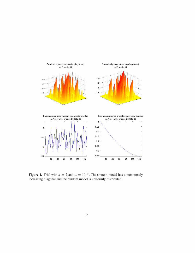
Figure 1. Trial with n = 7 and µ = 10−5. The smooth model has a monotonelyincreasing diagonal and the random model is uniformly distributed.

19

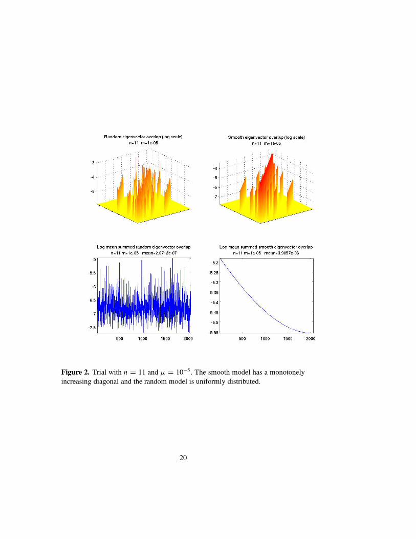
Figure 2. Trial with n = 11 and µ = 10−5. The smooth model has a monotonelyincreasing diagonal and the random model is uniformly distributed.

20

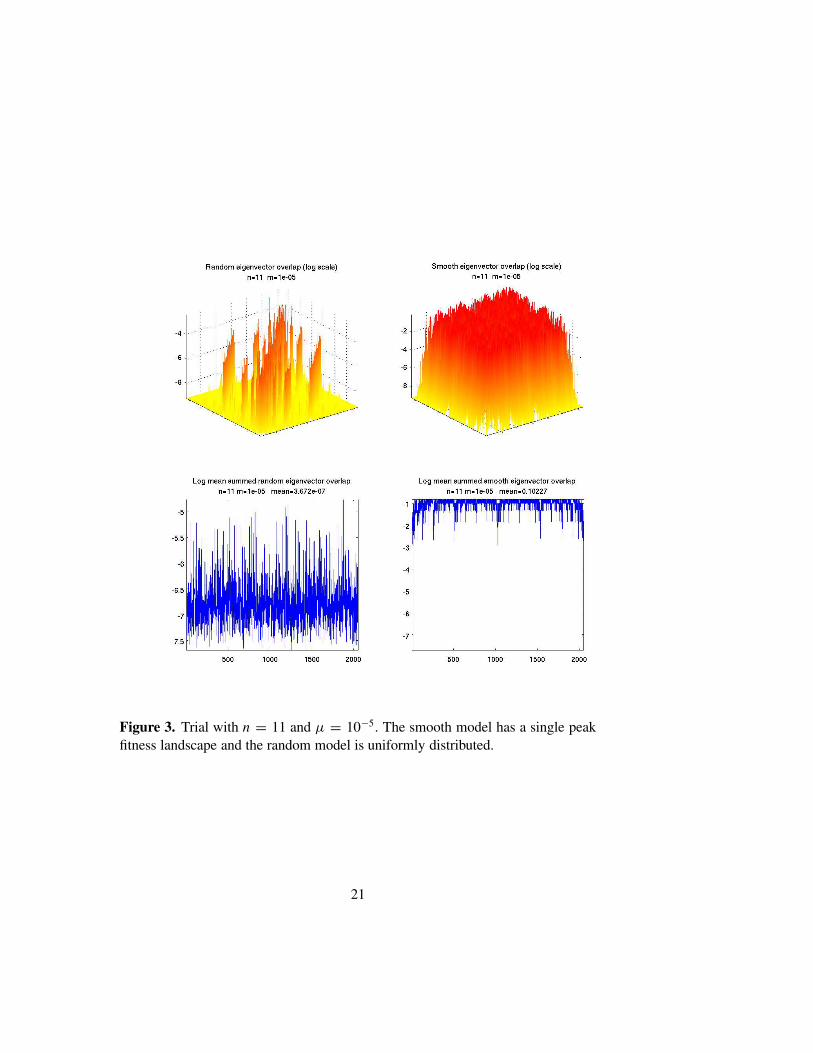
Figure 3. Trial with n = 11 and µ = 10−5. The smooth model has a single peakfitness landscape and the random model is uniformly distributed.

21

200 400 600 800 1000 1200 1400 1600 1800 2000

0.1

0.2

0.3

0.4

0.5

0.6

0.7

0.8

0.9

1Random spectrum, n=11 m=1e−05

(a) Spectrum of a randommodel.

200 400 600 800 1000 1200 1400 1600 1800 2000

0.1

0.2

0.3

0.4

0.5

0.6

0.7

0.8

0.9

Smooth spectrum, n=11 m=1e−05

(b) Spectrum of a modelwith monotone replica-tion matrix.

200 400 600 800 1000 1200 1400 1600 1800 20000.1

0.2

0.3

0.4

0.5

0.6

0.7

0.8

0.9

Smooth spectrum, n=11 m=1e−05

(c) Spectrum of a one-peak model.

Figure 4. The spectra of a random model, a monotone increasing model and aone-peak model with n = 11 and µ = 10−5.

0 200 400 600 800 1000 1200 1400 1600 1800 2000−1

−0.8

−0.6

−0.4

−0.2

0

0.2

0.4

0.6

0.8

1

Figure 5. The first 10 eigenvectors (corresponding to the 10 largest eigenvalues)of a random model with n = 11 and µ = 10−5. There are, apparently, only 9 peaksas, eigenvectors 2 and 4 have considerable overlap.

22

200 400 600 800 1000

−4.2

−4

−3.8

−3.6

−3.4

−3.2

−3

−2.8

−2.6

Log mean summed random eigenvector overlapn=10 m=0.01 mean=0.00059417

200 400 600 800 1000

−2.3

−2.25

−2.2

−2.15

−2.1

−2.05

−2

−1.95

Log mean summed smooth eigenvector overlapn=10 m=0.01 mean=0.006878

(a) n = 10, µ = 10−2.

200 400 600 800 1000

−7

−6.5

−6

−5.5

−5

−4.5

Log mean summed random eigenvector overlapn=10 m=1e−05 mean=9.2298e−07

200 400 600 800 1000

−5.5

−5.45

−5.4

−5.35

−5.3

−5.25

−5.2

−5.15

Log mean summed smooth eigenvector overlapn=10 m=1e−05 mean=4.2894e−06

(b) n = 10, µ = 10−5.

200 400 600 800 1000

−10

−9.5

−9

−8.5

−8

−7.5

Log mean summed random eigenvector overlapn=10 m=1e−08 mean=6.8859e−10

200 400 600 800 1000

−8.5

−8.45

−8.4

−8.35

−8.3

−8.25

−8.2

−8.15

Log mean summed smooth eigenvector overlapn=10 m=1e−08 mean=4.2827e−09

(c) n = 10, µ = 10−8.

200 400 600 800 1000

−13

−12.5

−12

−11.5

−11

−10.5

−10

Log mean summed random eigenvector overlapn=10 m=1e−11 mean=1.145e−12

200 400 600 800 1000

−11.5

−11.45

−11.4

−11.35

−11.3

−11.25

−11.2

−11.15

Log mean summed smooth eigenvector overlapn=10 m=1e−11 mean=4.2842e−12

(d) n = 10, µ = 10−11.

Figure 6. The average summed overlap with different values of µ, shown on alog10-scale. A random replication matrix is shown on the left and model with amonotone increasing diagonal on the right.

23

10 20 30 40 50 60

1

2

3

4

5

6

7

8

(a) Random replication matrix

10 20 30 40 50 60

0.2

0.4

0.6

0.8

1

1.2

1.4

1.6

1.8

2

2.2

(b) Smooth monotone replication matrix

10 20 30 40 50 60

5

10

15

20

25

30

(c) Single peak replication matrix

Figure 7. The solution of the non-linear model, (29), with a variety of differentreplication matrices. The parameters are n = 6, µ = .001, b = .02, and P 0 =(1, . . . , 1). The energy E is selected so that L + E has 11 positive eigenvalues.

24

20 40 60 80 100 120

2

4

6

8

10

12

µ = .01

(a) µ = .01

20 40 60 80 100 120

1

2

3

4

5

6

µ = .1

(b) µ = .1

20 40 60 80 100 120

5

10

15

20

25

30

µ = 1

(c) µ = 1

20 40 60 80 100 120

50

100

150

200

250

µ=10

(d) µ = 10

Figure 8. The solution of the non-linear model, (29), with a variety of differentmutation rates. The parameters are n = 7, b = .02, P 0 = (1, . . . , 1), and µ asindicated. The energy E is selected so that L + E has 10 positive eigenvalues.

25