The Effect of Ownership Structure on Prices in Geographically Differentiated Industries1

Raphael Thomadsen

Graduate School of Business Columbia University

August 30, 2004

Abstract This paper analyzes the joint empirical relationship between ownership structure and market geography on prices in the fast food industry. I estimate a model of demand and supply that accounts for the market geography, and use the estimated model to run counterfactual experiments that demonstrate how mergers between franchisees affects prices. I find that the impact of mergers can be large, that this impact decreases as the merging outlets are farther apart, that mergers among market leaders tend to increase prices more than mergers among weaker firms, and that mergers can still lead to higher prices even if the outlets are so far apart that, prior to the merger, each outlet’s presence does not affect prices at the other.

1. INTRODUCTION

This paper examines how the price impact of mergers among franchisees in the Santa

Clara County, California fast food industry varies according to the outlets’ proximity to each

other and to competitors. The price impacts from these mergers are similar to the ones that the

FTC examines when they are deciding whether to require merging retail companies, such as

grocery stores or movie theaters, to divest themselves of key outlets. I first present regression

estimates that demonstrate links between ownership structure, market geography, and prices. I

then measure the impact that joint ownership has on price under different market conditions by

estimating a model of demand and supply that is consistent with economic theory and accounts

for the geographic locations of all firms in the market, and then using the fitted model to conduct

counterfactual experiments that demonstrate how geographic differentiation affects the pricing

incentives of firms under different ownership structures.

The data I use consist of the prices, locations and outlet attributes of every Burger King

and McDonald’s outlet in Santa Clara County, California. As is common in many industries, it is

difficult to obtain quantity data because the firms keep this information as proprietary data, while

price data is easy to obtain because the econometrician can pose as a consumer.2 Building on the

work of Feenstra and Levinsohn (1995), I accommodate the fact that this quantity data was not

available by using the assumption of utility maximization by consumers to get a relationship

between price and quantity, and then substituting this relationship into the firms’ first-order

conditions from static Bertrand competition to jointly estimate the parameters of the indirect

utility functions of consumers and the marginal costs of firms.

The results show that mergers between McDonald’s franchisees can significantly increase

prices. For example, a McDonald’s in my sample set is shown to have a price that is 70¢ higher

than it would have been if the outlet had been independently operated. While mergers have a

greater effect on prices when the co-owned outlets are closer together rather than far apart, I also

1

find that prices increase from mergers among outlets that are far enough apart that each outlet’s

presence would have no impact on the other outlet’s prices under separate ownership. This

suggests that examining whether existing outlets impact the prices in other nearby outlets is an

insufficient test of a merger’s impact. I also find that mergers between Burger King outlets have

smaller effects on prices than mergers between McDonald’s outlets have, suggesting that anti-

trust authorities should focus mainly on mergers among dominant firms.

The rest of the paper proceeds as follows. Section 2 describes the industry, data and

results of descriptive regressions. Section 3 presents the model and the estimation procedure.

Section 4 reports the estimation results and analysis through the counterfactual experiments.

Finally, section 5 concludes.

2. DATA AND DESCRIPTIVE ANALYSIS

2.1 THE FAST FOOD INDUSTRY

McDonald’s and Burger King are the two largest fast food chains (in terms of annual

revenue) in the United States; together, they sell $30 billion of food in the US and $50 billion

worldwide each year. Almost 6 percent of the people in my study area consume a meal from

McDonald’s each day,3 and each year over 80 percent of Americans eat at a McDonald’s.

While both McDonald’s and Burger King Corporations own and operate many of their

own outlets, most of the outlets in the US are operated by franchisees.4 These franchisees operate

largely as independent businesses within a framework of a national brand, for which they pay a

fixed franchise fee plus a percentage of revenues to the franchisor. Lafontaine (1992) and

Lafontaine and Slade (1997) note that a given franchisor tends to offer the same contract terms to

each of the potential franchisees at a given point in time. In general, franchisees for these chains

are initially only allowed to own a single outlet. However, the fast food chains award additional

outlets to franchisees who perform well and maintain the standards that the chain specifies.5

2

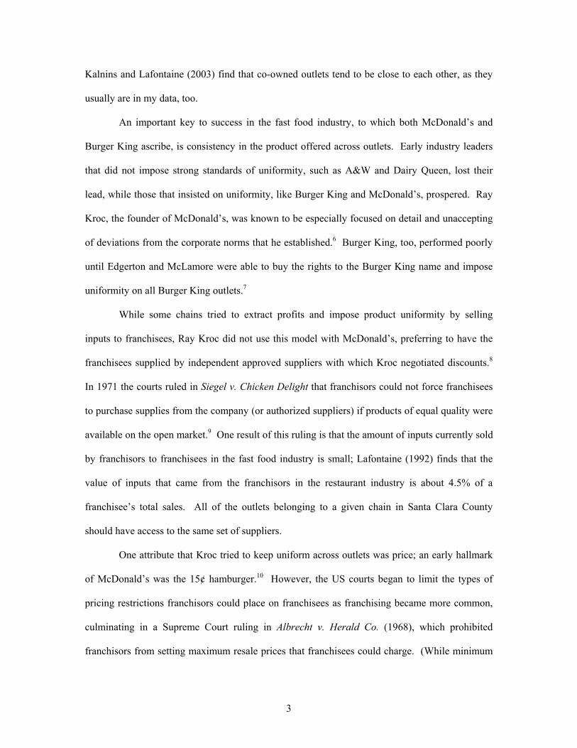
Kalnins and Lafontaine (2003) find that co-owned outlets tend to be close to each other, as they

usually are in my data, too.

An important key to success in the fast food industry, to which both McDonald’s and

Burger King ascribe, is consistency in the product offered across outlets. Early industry leaders

that did not impose strong standards of uniformity, such as A&W and Dairy Queen, lost their

lead, while those that insisted on uniformity, like Burger King and McDonald’s, prospered. Ray

Kroc, the founder of McDonald’s, was known to be especially focused on detail and unaccepting

of deviations from the corporate norms that he established.6 Burger King, too, performed poorly

until Edgerton and McLamore were able to buy the rights to the Burger King name and impose

uniformity on all Burger King outlets.7

While some chains tried to extract profits and impose product uniformity by selling

inputs to franchisees, Ray Kroc did not use this model with McDonald’s, preferring to have the

franchisees supplied by independent approved suppliers with which Kroc negotiated discounts.8

In 1971 the courts ruled in Siegel v. Chicken Delight that franchisors could not force franchisees

to purchase supplies from the company (or authorized suppliers) if products of equal quality were

available on the open market.9 One result of this ruling is that the amount of inputs currently sold

by franchisors to franchisees in the fast food industry is small; Lafontaine (1992) finds that the

value of inputs that came from the franchisors in the restaurant industry is about 4.5% of a

franchisee’s total sales. All of the outlets belonging to a given chain in Santa Clara County

should have access to the same set of suppliers.

One attribute that Kroc tried to keep uniform across outlets was price; an early hallmark

of McDonald’s was the 15¢ hamburger.10 However, the US courts began to limit the types of

pricing restrictions franchisors could place on franchisees as franchising became more common,

culminating in a Supreme Court ruling in Albrecht v. Herald Co. (1968), which prohibited

franchisors from setting maximum resale prices that franchisees could charge. (While minimum

3

resale price restrictions are also illegal, these constraints have generally not been the focus of the

industry.11) The Supreme Court relaxed the Albrecht decision in its 1997 State Oil Company v.

Khan decision, ruling that maximal resale price maintenance agreements should be tested by the

rule of reason rather than be illegal per se. While this decision occurred before I collected prices

in 1999, it appears that Burger King and McDonald’s did not try to re-impose setting prices,

likely because this would have entailed renegotiating all of the franchise agreements.12 This is

consistent with Lafontaine and Shaw’s (1999) finding that franchise contract terms are rarely

renegotiated within the contract period (typically 20 years).

2.2 THE DATA

This study uses an original dataset, collected over the summer of 1999,13 of the locations,

menu prices, presence of drive-thrus and playlands, and ownership of all fast food restaurants

belonging to chains in Santa Clara County, California, including all 64 McDonald’s and 39

Burger Kings in the county.14 I focus on competition between Burger King and McDonald’s, but

use the full dataset to confirm the validity of limiting the market to these two chains.

I focus on the pricing decisions of the franchised McDonald’s and Burger Kings, and not

those of the 21 outlets owned by McDonald’s corporation,15 because corporate outlets face

different incentives than franchised outlets, largely because the parent chain profits from sales at

every McDonald's outlet, giving them weaker incentives to steal business from franchisees and

stronger incentives to keep prices low to add an image of value to the McDonald’s brand as a

whole. The hypothesis that McDonald’s corporation’s incentives are different than those of their

franchisees is consistent with the results found in Lafontaine and Slade (1997), which finds that

corporate outlets tend to have lower prices than franchisee-owned outlets in their summary of the

findings of many academic studies on the topic. This result is also found in my data: 18 of the 21

McDonald’s-owned outlets in my dataset charge $2.99 for their Big Mac meal, the minimum

4

price observed in the market, while only 2 of the 43 franchised outlets charge this price.

I also completely omit from the market the outlets located in the San Jose airport,16 and

the McDonald’s located on the Moffett Air Force Base, because I believe that these outlets do not

compete with other fast food firms in the same manner as the other firms in my market. The

estimates in this paper are based on the pricing conditions of the 79 outlets (38 Burger Kings and

41 McDonald’s) remaining after accounting for these special cases.

The prices used for this study are the prices of the value meals with the signature

sandwich for each chain: the Whopper for Burger King and the Big Mac for McDonald’s. I use

these prices because these items are the most purchased items, and I was not able to obtain data

about the distribution of sales across all of the menu items.17,18 Table 1 presents summary

statistics of the price variation within these two chains (and of the other variables used in this

paper). Prices for Whopper meals range from $3.19 to $3.69, with a mean of $3.26 and a

standard deviation of 11¢. Big Mac meals vary in price from $2.99 to $4.09, with a mean of

$3.46 and a standard deviation of 27¢.

I supplement the firm data with demographic data, including the population density, age

distribution, racial distribution, gender distribution and median income of each census block-

group. I also have the locations where people work by traffic analysis zones (or TAZs), which

are areas defined locally and used by the US Department of Transportation. On average, the

TAZs are about three times the size of a block-group, although some TAZs are smaller than

block-groups. Finally, I have the locations of the 8 major malls in Santa Clara County.

2.3 DESCRIPTIVE ANALYSIS

The descriptive regressions reported in Table 2 show that geography and ownership

structure affects prices. The regressions demonstrate that prices decrease as the number of

competing McDonald’s or Burger King outlets in the area increase, and that outlets held by

5

franchisees that own other nearby franchises charge higher prices than independent franchisees.

The regressions also show that outlets belonging to hamburger chains other than McDonald’s or

Burger King do not affect the prices charged by McDonald’s or Burger King.

Column 1 in Table 2 gives the result from the regression of log-price on the number of

competing outlets (McDonald’s and Burger Kings owned by different parties) and number of co-

owned outlets located within 2 miles of the outlet,19 along with variables describing whether the

outlet is in a mall or has a drive-thru or playland. I also control for local demographics, including

the density of residents and workers within two miles of the outlet, the fraction of the residential

population within 2 miles that is made up of children, the fraction aged 30 – 64, the fraction older

than 64 years old, the fraction that is black, and the fraction that is male. The signs of most of the

coefficients on the variables are as expected: the presence of competitors within two miles of the

outlet reduces prices, while the presence of an outlet under the same ownership leads to higher

prices. The coefficient on the mall dummy variable is not significant, reflecting the fact that

about half of the outlets in malls have prices that are above the average price for the chain while

the other half have prices below the average for the chain. The coefficients on the drive-thru and

playland variables are insignificant and slightly negative, reflecting that the average prices in

outlets with a drive-thru or a playland are the same or somewhat below, respectively, the average

prices of the chain. However, since the coefficients on the drive-thru and playland variables are

always insignificant, and the signs of these variables change across different models,20 I interpret

these results as suggesting that these variables do not have a significant impact on price.

While the signs on the competition variables match economic intuition, the t-statistic on

the coefficient for competing McDonald’s and Burger Kings within 2 miles of the outlet is only

1.3. However, counting the number of outlets within a given distance of an outlet is not the only

way to measure an outlet’s competitive environment. Column 2 gives the regression results from

a similar model, except the level of competition is now measured by including the distance to the

6

nearest competing outlet, a dummy variable indicating whether the owner of the outlet owns any

other outlets, the distance to the closest such outlet if one exists, and the number of directions in

which other outlets within 2 miles are located.21 As in column 1, the signs of these coefficients

generally match expectations: prices increase as competitors are further away, decrease as outlets

are located in more directions, and co-ownership increases prices, but less and less as the co-

owned outlets are further apart.

The regressions reported in columns 3 and 4 are the same as the regressions in columns 1

and 2, respectively, except they include some additional demographic variables about the

population located within 2 miles of the outlet: their median income, the fraction that are Asian,

and the fraction that are Hispanic. All of these coefficients are insignificant (with t-statistics at or

below 0.82). This justifies omitting income or race variables other than black in the structural

model I present and estimate later in this paper.

The regressions in columns 5 and 6 support designating McDonald’s and Burger King as

the relevant market. These regressions include the number of outlets belonging to other

hamburger chains within 2 miles of the outlet in column 5, and the distance to the closest outlet

belonging to other hamburger chains in column 6. In column 5, the coefficient on the number of

other hamburger outlets variable is small – about half the size of the coefficient on other

McDonald’s or other Burger Kings – and insignificant, with a t-statistic is just below 0.5. A

similar result is obtained in regression 6; the coefficient on the other hamburger variable is again

statistically insignificant, and the sign of the coefficient is the opposite of that which would be

expected from a competitor.22 These results are consistent with Kalnins (2003), which finds that

the relevant sets of competitors in the hamburger segment are smaller subsets of competitors, and

that other franchisees belonging to the same chain are often an outlet’s strongest competitor.

3. THE MODEL

7

While the descriptive regressions reported in Section 2.3 demonstrate a correlation

between the ownership structure of firms and prices, they have two flaws. First, the measures of

competitors used above are ad hoc, and it is impossible to account for the full richness of the

layout of firms in the market in such a regression. For example, an outlet’s equilibrium prices

will be different if there are two competitors located one-half mile away from the outlet but

located adjacent to each other than if the two competitors were located one-half a mile away but

on opposite sides of the outlet. One could add a dummy variable to the regression to differentiate

these two cases, but there are numerous potential market layouts and generally it will be

impossible to account for every layout using a real dataset. Also, in a large market such as Santa

Clara County it is not clear which outlets are close enough to be relevant competitors. Rather

than imposing an ex ante restriction on the set of competitors, it would be preferable to use

economic foundations to allow the data to determine who the relevant set of competitors are.

The second flaw is that while regression results can establish that prices are higher at

outlets owned by franchisees that own other proximate franchises and at those outlets that are

further away from competing outlets, they cannot be used to calculate what prices would be for

these outlets under different ownership structures because they do not establish a causal

relationship between prices and market structure. It is possible that this conditional correlation is

instead a result of common factors that affect both variables. Thus, the econometrician cannot

know whether the conditional correlations will remain after the economic environment is

changed. This problem is larger for cross-sectional analysis than for panel analysis because a

panel allows the econometrician to control for persistent common factors. However,

counterfactual prediction with panel regressions is still problematic if there are common factors

that vary over time or omitted common factors that affect the choice of which outlets have

changes in ownership.23

I address both of these concerns by estimating a model of supply and demand that is

8

consistent with economic theory, accounts for the true locations and ownership structure of firms,

and allows the data to reveal which firms are de facto competitors. I then conduct counterfactual

experiments with the fitted model to demonstrate how geography and ownership patterns jointly

affect prices. This approach of measuring merger impact by examining the differences in pricing

incentives of merged vs. independent firms has become common practice. (E.g., see Nevo’s

(2000) analysis of cereal mergers, or Dube’s (2004)’s study of soft drink mergers.)

This section outlines the model and estimation procedure, and Section 4 presents the

estimates and analysis. The approach used in this paper follows work by Bresnahan (1987),

Berry (1994) and Berry, Levinsohn and Pakes (1995) (hereafter BLP) that demonstrates how to

estimate utilities and costs in differentiated industries from aggregate data. Demand is modeled

as being derived from consumers making a discrete choice of where to purchase their meal.24

Consumers each choose to consume a representative meal at the outlet that delivers the maximum

utility. Geography is incorporated into the demand-side of the model following Davis (2001),

who added geography to the BLP framework in his study on the welfare effects of movie theater

locations. The supply of fast food meals is modeled by assuming that each franchisee faces a

constant marginal cost of producing meals and maximizes their profits by setting prices at each of

their outlets, which compete through static Bertrand competition. As in Bresnahan (1987) and

BLP, firm marginal costs are estimated as parameters rather than derived from cost data.

Similar to Feenstra and Levinsohn (1995), I estimate the model using only price data and

not quantity data. This is possible because both the parameterized utility functions from the

demand side of the model and the first order conditions for each franchisee on the supply side

provide relationships between observed prices and implied quantities that jointly identify the

parameters of the model. This approach gives estimates that are less efficient than one could

obtain if accurate quantity data were available.25 However, quantity data is often not available

because the firm keeps it a secret, which is the case for my dataset. On the other hand, price data

9

can be easier to collect because the econometrician can often pose as a customer.26

3.1 DEMAND

Demand for fast food meals at each of the outlets is modeled using a discrete-choice

framework.27 Consumers choose either to purchase their meal from one of the J fast food outlets

or to consume an outside good. Consumers are spread across the county, but have the same

utility function except for differences from different demographic attributes and from different

unobserved tastes for each location/chain combination. Note that although consumers can choose

to eat at any outlet in the county, they de facto choose between those close to their location

because of their disutility for travel. Thus, proximate restaurants are closer substitutes than

outlets that are further away.

Formally, the conditional indirect utility of consumer i from fast food outlet j is

(1A) jijjijji PDXV ,,, ηγδβ +−−′=

where Xj is a vector of dummies indicating (i) the chain to which outlet j belongs, (ii) whether

there is a drive-thru or a playland in the outlet, and (iii) whether the outlet is located in a mall, Di,j

is the distance between consumer i and outlet j,28 Pj is the price of a meal at outlet j, β, δ, γ are

parameters to be estimated, and ηi,j is the unobserved portion of utility for individual i at outlet j.

If the consumer instead consumes only the outside good, their indirect utility is then:

(1B) 0,00, iii MV ηπβ ++= ,

where Mi is a vector of the consumer’s age, gender and race. β0 is normalized to be 0.

I account for the different physical product characteristics of the food at the different

chains through the chain dummies that appear in the indirect utility function. Product

differentiation papers have traditionally accommodated physical differences by defining utilities

over each of the product attributes. However, these papers also note that equilibrium prices

10

depend both on the observable product attributes and on the product attributes that are

unobserved by the econometrician but observed by the firms and consumers.

I can circumvent this problem because a chain’s food is nearly identical at each of its

restaurants, allowing me to get multiple observations of the same item in a variety of competitive

environments. Note that not only is the food identical, but the chains also try to make the

experiences at each of their outlets identical. For example, their outlets have a uniform

appearance, their menu boards look very similar, and their workers wear similar uniforms.29

Also, both the descriptive analysis and my estimated demand model show that even significant

product attributes such as the presence of a playland or drive-thru, or whether an outlet is located

in a mall, have minimal impacts on prices, reinforcing the idea that small unobservable

differences are probably not driving differences in prices.

I exploit this homogeneity by estimating a fixed effect for each chain’s food in a similar

manner as Nevo (2001), who also observes identical products in a variety of competitive

environments. This fixed effect captures the total utility for the food at each chain, including

utility from unobservable attributes, including advertising, brand image, and Pokemon toys.

The consumer will purchase one meal from the restaurant that delivers the highest utility

unless the outside good provides an even greater utility. Given this utility function and ( )if η ,

the probability density of the (J+1)-dimensional vector ηi, the share of consumers located in a

particular location, b, and demographic type, M, who consume from outlet j is:

(2) ( ) ( ) iA

ibj dfMXPSj

ηηπγδβ ∫=,,,|,,,

where P is the J-dimensional vector of prices for every outlet in the market, and

)()(| 0,,,, ijitijiij VVjtVVA >∩≠∀>= η

is the set of match values, ηi, between consumers and outlets such that the consumer derives a

higher utility by consuming from outlet j than from any other outlet t or from the outside good. I

assume that ηi has an i.i.d. type I extreme-value distribution. Thus, the fraction of consumers of

11

demographic type M located in location b who choose to purchase a meal from outlet j is:

(3)

∑=

′

′

+= J

t

P-D-XM

P-D-X

bj,ttb,t

jjb,j

ee

e),,,|MX,,P(S

1

γδβπ

γδβ

πγδβ .

I discretize the consumers' locations and sum over the decisions of consumers at each

location.30 I consider two types of consumers: residential consumers and workers at their work

locations. Residential consumers live in one of 1020 census block-groups. These block-groups

are relatively small areas, and I place all of residents at the block-group’s centroid. My worker

data places workers in one of 479 areas called traffic analysis zones, or TAZs. As noted in

Section 2.2, these are generally, but not always, larger than census block-groups. For TAZs that

are smaller than census block-groups, I place the workers at the centroid of that TAZ. For TAZs

that are larger then block-groups, I place the workers at the centroids of the internal block-groups,

assigning each location a fraction of the workers in the TAZ that is proportionate to the areas of

the different block-groups. This yields 1093 different worker locations.

Total demand for each outlet is then calculated by summing the product of the fraction of

consumers of demographic M and location b who patronize the outlet and the mass of consumers

of that demographic at that location, h(b,M) across all demographic-location pairs:

(4) . ∑∑=b M

bjj ,,,|MX,,PSMbh,,,|X,PQ )(),()( , πγδβπγδβ

The derivative of demand with respect to price is computed in a similar manner:

(5) ∑∑ ∂

∂=

∂

∂

b M k

bj

k

j

P,,,|MX,,PS

MbhP

,,,|X,PQ )(),(

)( , πγδβπγδβ

3.2 SUPPLY

I model the supply of fast food by assuming that franchisees set prices at each of their

outlets in a way that maximizes the joint profits of all of their outlets according to a static

Bertrand game. This assumption is reasonable because the firms offer to sell as many units as are

12

demanded at the posted prices, and because the firms can change their prices quickly and easily.

The major costs for these firms include rent, equipment and other capital, labor, food,

paper (and other materials for food containers) and payments to the franchisor. Payments to the

franchisor consist of a combination of a fixed component and a percentage of revenues. The

equipment and capital are fixed costs, while labor, food and paper costs vary according to the

number of meals sold. Labor is adjusted not just for the expected demand, such as having more

workers during lunch hours compared to the late afternoon times, but firms also attempt to adjust

labor according to the realized demand by calling in more workers on unexpectedly busy days

and sending workers home early on unexpectedly low volume days.31

Formally, there are F firms (franchisees), each owning a subset Ff of the j = 1,…, J

outlets. I assume that each firm’s costs consist of fixed costs plus a constant marginal cost for

each unit. The profits to firm f are then

(6) ∑∈

−−=∏fFj

jjjjjkf FCPQcPQPr ))()((

where FCj is the fixed cost of operating outlet j, cj is the marginal cost of a meal at outlet j, rk is

the fraction of revenue that the franchisees belonging to chain k retain after paying their franchise

royalties, and P is the J-dimensional vector of prices for every outlet.32 Note that maximizing (6)

is the same as maximizing

(7) ∑∈

−⎟⎟⎠

⎞⎜⎜⎝

⎛−=∏

fFj k

jj

k

jjjf r

FCPQ

rc

PQP ))()(( .

I refer to k

jj r

cC = as the marginal cost, since the firms will be acting as if they are maximizing

profits with marginal costs of Cj.

I assume that each outlet’s marginal cost is equal to a chain-specific marginal cost plus a

zero-mean unobservable component. Thus, outlet j’s marginal cost is

(8) Cj = (Ck + ε j)

13

where Ck represents the mean marginal cost for all outlets belonging to chain k, and ε j represents

the zero-mean, outlet-specific, portion of marginal costs.33 The different chains will have

different marginal costs because they serve different food. I attribute the outlet-specific

component of marginal cost to be due to the labor efficiency of the workers and the management

of the outlet because the other sources of variable costs, food and materials, are very standard

across all of the outlets.34 The efficiency of the workers, on the other hand, varies with the

experience and ability of different individuals.35 I assume that the franchisee knows their true

marginal cost, including ε j, when they set their prices, but that this marginal cost is unobservable

to the econometrician.

Each firm maximizes the profit function in equation (7), yielding the following first-order

conditions for the price at each outlet:

(9) 0)(

)()( =∂

∂−−+ ∑

∈ j

r

Frrkrj P

PQCPPQ

f

ε

These J equations can be solved for each εj. To do this, define a matrix Ω as

(10) ⎪⎩

⎪⎨⎧

∂∂

=Ω.otherwise0,

ownersamethehaveandif,,

jrPQ

j

r

rj

This implies that the first-order conditions can be rewritten as

(11) 0)()( =−−Ω+ εCPPQ

where Q(P), C and ε are the vectors of quantities of each of the outlets, the chain-specific

marginal costs, and outlet-specific marginal costs, respectively.

While I do not have data on quantity and the derivative of quantity with respect to price,

these variables were solved as a function of the utility parameters in section 3.1. Substituting

these quantities and derivatives into equation (11) yields

(12) 0)()()( =−−Ω+ εθθ CP|X,P|X,PQ

where ),,,( πδγβθ ′′′′=′ . This can be rearranged to solve for the vector of residuals for

14

Generalized Method of Moments (hereafter GMM) estimation:

(13) ( ) ( )θθε |,|, 1 XPQXPCP −Ω+−= ,

3.3 ESTIMATION

Appropriate instruments, Z, will be uncorrelated with ε j, but correlated with the cost or

demand terms. A sufficient condition for the latter requirement is that

(14) E[ε j(θ*)|Zj] = 0,

where θ* is the true value of θ.

The first instruments I use are chain dummies, which shift the costs of the outlet.36 The

unobserved components of costs are, by assumption, independent of the chain affiliation of the

outlet, but the chain dummies will be correlated with the marginal costs of the outlet.

The remaining instruments are demand shifters. The first demand shifters are the

distance to the nearest outlet and the number of directions from the outlet in which there are other

outlets within 2 miles.37 I assume that these instruments are uncorrelated with the unobserved

components of cost.38 BLP suggest one way that this can be justified: assume that the ε’s evolve

as a first-order Markov process, where the innovation in that process is independent of the

outlet’s proximity to competitors. This assumption is reasonable in the fast food industry due to

the high rate of employee and managerial turnover, which is often over 100%.39 In this case, the

level of ε observed at the time that the data was collected would be independent of the level of ε

that existed when the firm entered the market.

The next set of instruments are dummy variables indicating the presence of observable

traits of the outlets – whether the outlet is located in a mall or has a drive-thru or a playland –

which are included in consumers’ utility functions in case they have an impact on the outlets’

demand. The final set of instruments consists of demographic data for each of the outlets. These

are the population density in the nearest census block-group and the density of workers in the

15

closest TAZ. These factors shift demand because, all else equal, sales increase when firms are

located near a cluster of potential customers.40

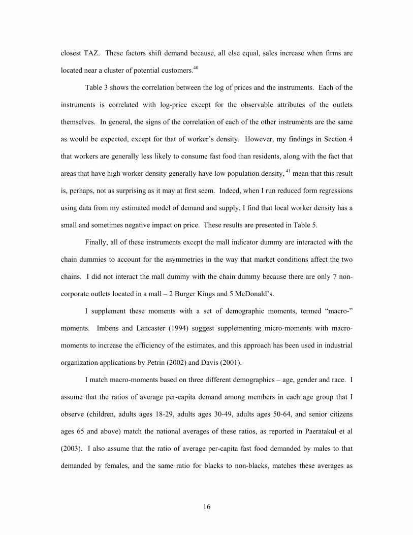
Table 3 shows the correlation between the log of prices and the instruments. Each of the

instruments is correlated with log-price except for the observable attributes of the outlets

themselves. In general, the signs of the correlation of each of the other instruments are the same

as would be expected, except for that of worker’s density. However, my findings in Section 4

that workers are generally less likely to consume fast food than residents, along with the fact that

areas that have high worker density generally have low population density, 41 mean that this result

is, perhaps, not as surprising as it may at first seem. Indeed, when I run reduced form regressions

using data from my estimated model of demand and supply, I find that local worker density has a

small and sometimes negative impact on price. These results are presented in Table 5.

Finally, all of these instruments except the mall indicator dummy are interacted with the

chain dummies to account for the asymmetries in the way that market conditions affect the two

chains. I did not interact the mall dummy with the chain dummy because there are only 7 non-

corporate outlets located in a mall – 2 Burger Kings and 5 McDonald’s.

I supplement these moments with a set of demographic moments, termed “macro-”

moments. Imbens and Lancaster (1994) suggest supplementing micro-moments with macro-

moments to increase the efficiency of the estimates, and this approach has been used in industrial

organization applications by Petrin (2002) and Davis (2001).

I match macro-moments based on three different demographics – age, gender and race. I

assume that the ratios of average per-capita demand among members in each age group that I

observe (children, adults ages 18-29, adults ages 30-49, adults ages 50-64, and senior citizens

ages 65 and above) match the national averages of these ratios, as reported in Paeratakul et al

(2003). I also assume that the ratio of average per-capita fast food demanded by males to that

demanded by females, and the same ratio for blacks to non-blacks, matches these averages as

16

reported in the same article.

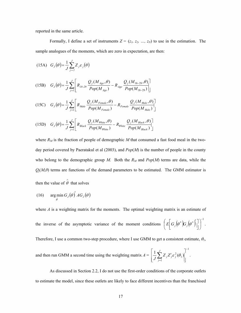
Formally, I define a set of instruments Z = (z1, z2, …, zN) to use in the estimation. The

sample analogues of the moments, which are zero in expectation, are then:

(15A) ( ) ( )∑=

=J

1 j jjJ θZ

JG εθ 1

(15B) ( ) ∑= −

−

⎥⎥⎦

⎤

⎢⎢⎣

⎡−=

J

j

jAge

Age

Agej29-18J MPop

MQR

MPopMQ

RJ

G1 2918

2918

)(),(

)(),(1 θθ

θ

(15C) ( ) ∑=

⎥⎦

⎤⎢⎣

⎡−=

J

j Male

MalejFemale

Female

FemalejMaleJ MPop

MQR

MPopMQ

RJ

G1 )(

),()(),(1 θθ

θ

(15D) ( ) ∑=

⎥⎦

⎤⎢⎣

⎡−=

J

j Black

BlackjWhite

White

WhitejBlackJ MPop

MQR

MPopMQ

RJ

G1 )(

),()(),(1 θθ

θ

where RM is the fraction of people of demographic M that consumed a fast food meal in the two-

day period covered by Paeratakul et al (2003), and Pop(M) is the number of people in the county

who belong to the demographic group M. Both the RM and Pop(M) terms are data, while the

Qj(M,θ) terms are functions of the demand parameters to be estimated. The GMM estimator is

then the value of that solves ∧θ

(16) ( ) ( )θθθ

JJ AGG ′ˆminarg

where A is a weighting matrix for the moments. The optimal weighting matrix is an estimate of

the inverse of the asymptotic variance of the moment conditions .

Therefore, I use a common two-step procedure, where I use GMM to get a consistent estimate, θ

( ) ( )1

**−

⎟⎠

⎞⎜⎝

⎛⎥⎦⎤

⎢⎣⎡ ′

θθ jj GGE

1,

and then run GMM a second time using the weighting matrix A = 1

11

2 )(1−

= ⎥⎥⎦

⎤

⎢⎢⎣

⎡′∑

J

jjjj ZZ

Jθε .

As discussed in Section 2.2, I do not use the first-order conditions of the corporate outlets

to estimate the model, since these outlets are likely to face different incentives than the franchised

17

outlets. Including the pricing decisions of firms whose objective functions are incorrectly

specified would introduce error that would destroy the consistency of the estimates. However, I

account for the effects that their prices and presence have on the demand for every other outlet in

the market because consumers typically do not distinguish between those outlets that are

corporate-owned or franchised (or even know which outlets are which).

Note that using only the first-order conditions of outlets owned by franchisees, and not

those of the parent corporation, does not introduce any sample selection bias into the estimates

because I am conditioning on firms that have similar incentives, rather than on the endogenous

variable, price (or ε ). The only potential loss from omitting pricing decisions of the corporate-

owned outlets is efficiency, because the ε j’s still retain their properties of being mean zero and

orthogonal to the instruments,42 while the instruments are still correlated with each outlet’s

demand and chain-specific marginal cost. However, since I am only using the pricing decisions

of franchised outlets, I can only claim to have estimated the marginal costs and behavior of

franchised outlets, and am unable to say anything about the costs or behavior of corporate outlets,

or run counterfactuals predicting how pricing would change if an outlet went from being

franchisee-operated to being corporate-operated.

3.4 IDENTIFICATION

The intuition behind the identification of the utility and cost functions comes from the

idea that while there may be more than one combination of parameter values that are consistent

with the observed equilibrium prices under some market structures, different sets of parameters

will lead to different equilibrium prices in other market conditions. For example, increasing both

the parameter for consumers’ base utility for a good and the parameter for price sensitivity could

keep the profit-maximizing price of the good in a monopoly market unchanged. However, the

changed price sensitivity would lead to an equilibrium where the firms would charge different

18

prices in a duopoly market than they would have charged if both of these parameters had been

smaller. The market structures used in this paper, where firms are closer and further away from

different sets of competitors, have a much richer set of substitution patterns than can be achieved

under the traditional market structures of monopoly, duopoly, etc ….

To see how both supply and demand effects are identified through the observed prices,

note that equation 13 can be solved for price:

(17) . ( ) ( ) εθθ +Ω−= − |,|, 1 XPQXPCP

Thus, price can be divided into two components. The first component, the cost component, will

not vary in different competitive environments, while the second term, the markup, which comes

from the demand for the product, will. Of course, it is also necessary that the rate of change in

the markup term as a function of market structure (in this case, geography) be unique in the

demand parameters in order for all of the parameters to be identified. The demand model

introduced in section 3.1 has this property.43,44

4. ANALYSIS

4.1 THE ESTIMATES

The estimates of the model are reported in Table 4. The first column reports the

estimates for the model described in Section 3, where consumers are located either at home or at

work and get different utilities for consumption at outlets in malls than from consumption at

stand-alone outlets. The second column reports the results for a similar model, with the only

difference being that, in the model reported in column 2, consumers are indifferent between

whether an outlet is located inside or outside of a mall, holding all other attributes of the outlet

constant. The model estimated in column 3 is the same as the one in column 2, except that some

consumers are located at each mall.45 Note that while the estimates vary somewhat across these

specifications, the important characteristics of the estimates remain the same, adding confidence

19

that the results are not dependent upon the exact specification of the model. Also, the p-values

for χ2 tests of over-identifying restrictions are 0.34 or less in each specification, so I conclude that

over-identification is not a problem.

Since all of the specifications give similar estimates, I focus on the estimates in column 1.

I assume that the model and assumptions presented in Section 3 are correct for the rest of the

analysis, and I use this fitted model in the counterfactual experiments.

Due to the covariance between the McDonald’s and Burger King baseline utility

estimates, the standard error of the difference between these variables is 0.96, implying that

McDonald’s gives a statistically significantly higher utility to consumers than Burger King.

Travel costs, which are equal to the coefficient of distance divided by the coefficient of price, are

estimated to be close to $3.00/mile. This travel cost estimate implies that consumers have an

average opportunity cost of their time of almost $27/hour.46

The estimated marginal costs indicate that the firms hold significant market power.47 The

estimates of marginal costs in column 1 imply that the average markups are $1.23 for Burger

King and $2.01 for McDonalds. These markups are even larger after accounting for the rate at

which the firms keep their revenues.48 The marginal cost estimates in Table 4 imply that the real

economic marginal costs for the outlets are $1.27 for McDonald’s and $1.86 for Burger King.

The estimated marginal costs seem to be consistent with other information I have on what

marginal costs should be: Emerson (1990) estimates that, on average, food and paper costs are

about 34% and 32% of sales for McDonald’s and Burger King, respectively, with this number

falling at about 15% over 10 years, and that labor costs are approximately 22% and 28% of sales

for these two firms. Discussions with other people familiar with the costs of running a fast food

outlet have given me similar numbers. Paper and food clearly belong as part of marginal costs. It

is more difficult to determine the fraction of labor costs that should be classified as marginal costs

because some labor costs are fixed costs. If the national averages apply to the market I study then

20

the real marginal costs would be in the range of $1.00 - $1.76 for McDonald’s, and $0.89 - $1.80

for Burger King, depending on the amount of labor costs that are allocated to marginal costs. My

estimate of $1.27 for McDonald’s falls within this range, while my estimate of $1.86 for Burger

King is just above it. However, the fact that retail prices and wages were higher in Silicon Valley

than in the rest of the country49 suggests that Emerson’s cost guide will not hold exactly in this

market.

To add confidence in the estimated model, Table 5 reports regression results where the

log of the predicted prices implied by the fitted model50 are regressed on the same regressors as in

columns 1 and 2 of Table 2. The estimates of the key competitive variables – the number of

competing and co-owned outlets within 2 miles, the distance to the closest competing and co-

owned outlets, and the number of directions in which nearby outlets are located – are of the same

order of magnitude as the estimates from the actual data. Also, the R-squareds of these

regressions are similar to the R-squareds in the regressions using the actual data.

Table 6 presents reports the own and cross-price elasticities for outlets surrounding the

Burger King located at 5154 Moorpark. A map of this area is presented in Figure 1. The cross-

price elasticities are larger for outlets located close together than for those located further apart.

Also, changes in prices at McDonald’s have much larger effects on the percent changes in

quantities at either McDonald’s or Burger King than changes in prices at Burger Kings have.51

4.2 EXPERIMENTS

I use the estimates from the model reported in column 1 of Table 4 to run counterfactual

experiments that demonstrate how ownership structure and location jointly affect prices. These

experiments demonstrate both that co-ownership can increase prices significantly, especially if

the co-owned outlets are close together, and that mergers can lead to increased prices even when

the merging outlets are far enough apart that the presence of the other outlet would have no

21

impact on price under separate ownership. The experiments also demonstrate that mergers

among McDonald’s outlets increase prices more than mergers among Burger Kings.

To see how the magnitude of a merger’s impact on prices is affected by the proximity of

the merging outlets, I contrast how two different mergers would change prices. The first merger I

consider is a merger between the McDonald’s located at 1935 Tully and the McDonald’s located

in the Eastridge Mall. These outlets are about ⅓ mile apart, and both are independently owned.

A merger between these outlets would increase prices at 1935 Tully by 29¢ (with a 95%

confidence interval of 5¢ to $1.04), from $3.19 to $3.48. This is larger than the price impact that

would result from a merger between the McDonald’s located at 5925 Almanden and the

McDonald’s located in the Oakridge Mall, which is located 1.25 miles away. The additional

distance between the outlets implies that the merger would increase prices at 5925 Almaden by

12¢ (2¢ to 35¢), from $3.39 to $3.51.52 While this price effect is smaller than the effect of the

merger between the outlets at 1935 Tully and Eastridge Mall, it is worth noting that the merger

between these owners would lead to the 12¢ increase in prices even though these outlets are far

enough apart that, given the presence of other competitors in the area, the presence of the outlet in

the Oakridge Mall53 has only a minimal effect on the price charged at 5925 Almaden under the

separate ownership structure that actually exists. That is, if the McDonald’s outlet located in the

Oakridge Mall (and all of the other outlets owned by the same owner) exited from the market, the

price of the Big Mac meal at 5925 Almaden would only increase by 1¢, from $3.39 to $3.40.

To understand how this can occur, consider the effects that a merger and an exit by a

competitor each have on an outlet’s pricing incentives. A merger creates an incentive to increase

prices as long as some of the outlet’s consumers will instead choose to patronize the other store,

allowing the owner to recapture some of the profits from these marginal consumers. On the other

hand, the exit of a competitor has two effects on an outlet’s pricing incentives. First, consumers

have one less alternative in their choice set, decreasing their price sensitivity. However, some of

22

the exiting outlet’s customers will switch to the remaining outlet. These customers tend to find

patronizing the remaining outlet to be less attractive relative to consuming the outside good than

the outlet’s original customers rate this relative attractiveness. If the outlets are far enough apart

then this last effect can offset the effect on price sensitivity from the decrease in choices. Thus,

the exit of a competitor has an ambiguous effect on an outlet’s demand elasticity,54 while a

merger can only cause prices to increase.

While the above experiments demonstrate the link between outlet proximity and the

magnitude of the price-impact of a merger, it is worth noting that mergers between outlets can

have even larger effects depending on the exact combination of market geography and ownership

structure involved. For example, the price at the outlet located at 952 El Monte, whose owner

owns several outlets in the vicinity, is 70¢ (31¢ to $1.46) higher than the price would be if it

outlet were instead operated under independent ownership.

I further demonstrate these findings – that mergers can have a large effect on price, that

the effect of mergers is larger among outlets that are closer together, and that a merger can lead to

increases in prices even when outlets are located far enough apart that the presence of the other

outlet would not decrease the outlet’s price under separate ownership – by running an experiment

in an artificial market. In this experiment, I place two McDonald’s into a 10x10 mile market with

a uniform distribution of consumers. I place one McDonald’s outlet at the center of the market. I

then place the other McDonald’s outlet at different distances away from the McDonald’s at the

center of the market and calculate the equilibrium prices for the McDonald’s at located at the

center of the market under joint and independent ownership structures. As a benchmark, if there

were only one McDonald’s in the market, and if it were located at the center of this market, then

this outlet would charge a monopoly price of $3.71.

Figure 2 graphs the equilibrium prices for the McDonald’s located at the center of such a

market as a function of the distance between it and the other outlet. Under separate ownership,

23

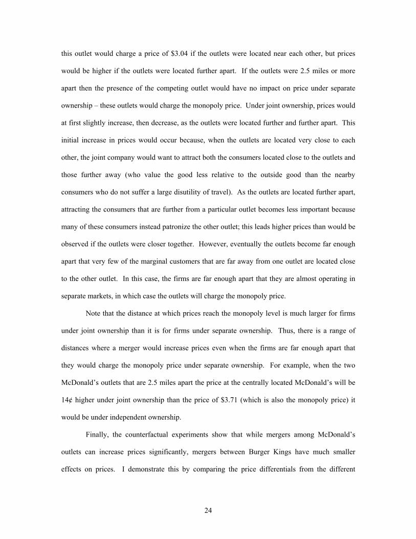
this outlet would charge a price of $3.04 if the outlets were located near each other, but prices

would be higher if the outlets were located further apart. If the outlets were 2.5 miles or more

apart then the presence of the competing outlet would have no impact on price under separate

ownership – these outlets would charge the monopoly price. Under joint ownership, prices would

at first slightly increase, then decrease, as the outlets were located further and further apart. This

initial increase in prices would occur because, when the outlets are located very close to each

other, the joint company would want to attract both the consumers located close to the outlets and

those further away (who value the good less relative to the outside good than the nearby

consumers who do not suffer a large disutility of travel). As the outlets are located further apart,

attracting the consumers that are further from a particular outlet becomes less important because

many of these consumers instead patronize the other outlet; this leads higher prices than would be

observed if the outlets were closer together. However, eventually the outlets become far enough

apart that very few of the marginal customers that are far away from one outlet are located close

to the other outlet. In this case, the firms are far enough apart that they are almost operating in

separate markets, in which case the outlets will charge the monopoly price.

Note that the distance at which prices reach the monopoly level is much larger for firms

under joint ownership than it is for firms under separate ownership. Thus, there is a range of

distances where a merger would increase prices even when the firms are far enough apart that

they would charge the monopoly price under separate ownership. For example, when the two

McDonald’s outlets that are 2.5 miles apart the price at the centrally located McDonald’s will be

14¢ higher under joint ownership than the price of $3.71 (which is also the monopoly price) it

would be under independent ownership.

Finally, the counterfactual experiments show that while mergers among McDonald’s

outlets can increase prices significantly, mergers between Burger Kings have much smaller

effects on prices. I demonstrate this by comparing the price differentials from the different

24

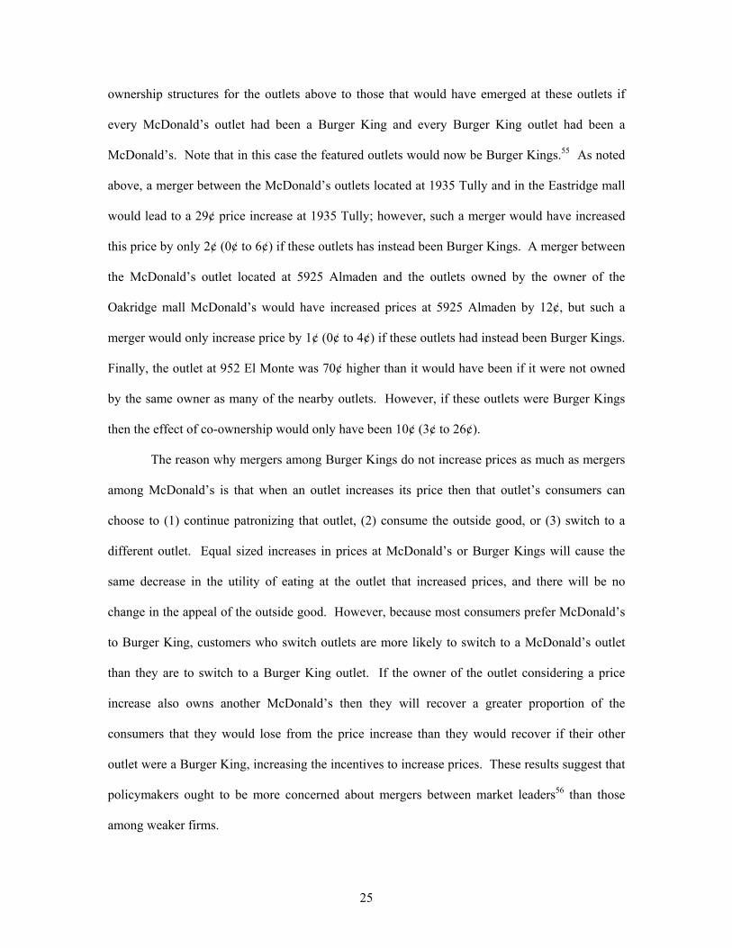
ownership structures for the outlets above to those that would have emerged at these outlets if

every McDonald’s outlet had been a Burger King and every Burger King outlet had been a

McDonald’s. Note that in this case the featured outlets would now be Burger Kings.55 As noted

above, a merger between the McDonald’s outlets located at 1935 Tully and in the Eastridge mall

would lead to a 29¢ price increase at 1935 Tully; however, such a merger would have increased

this price by only 2¢ (0¢ to 6¢) if these outlets has instead been Burger Kings. A merger between

the McDonald’s outlet located at 5925 Almaden and the outlets owned by the owner of the

Oakridge mall McDonald’s would have increased prices at 5925 Almaden by 12¢, but such a

merger would only increase price by 1¢ (0¢ to 4¢) if these outlets had instead been Burger Kings.

Finally, the outlet at 952 El Monte was 70¢ higher than it would have been if it were not owned

by the same owner as many of the nearby outlets. However, if these outlets were Burger Kings

then the effect of co-ownership would only have been 10¢ (3¢ to 26¢).

The reason why mergers among Burger Kings do not increase prices as much as mergers

among McDonald’s is that when an outlet increases its price then that outlet’s consumers can

choose to (1) continue patronizing that outlet, (2) consume the outside good, or (3) switch to a

different outlet. Equal sized increases in prices at McDonald’s or Burger Kings will cause the

same decrease in the utility of eating at the outlet that increased prices, and there will be no

change in the appeal of the outside good. However, because most consumers prefer McDonald’s

to Burger King, customers who switch outlets are more likely to switch to a McDonald’s outlet

than they are to switch to a Burger King outlet. If the owner of the outlet considering a price

increase also owns another McDonald’s then they will recover a greater proportion of the

consumers that they would lose from the price increase than they would recover if their other

outlet were a Burger King, increasing the incentives to increase prices. These results suggest that

policymakers ought to be more concerned about mergers between market leaders56 than those

among weaker firms.

25

5. CONCLUSION

This paper demonstrates how ownership structure and market geography jointly affect

prices that firms charge by examining pricing patterns in the fast food market of Santa Clara

County, California. First, descriptive regressions on the data demonstrate that there is a link

between ownership, location, and prices. Then, I estimate a model of supply and demand that

accounts for the actual layout of the firms. This fitted model is used to conduct counterfactual

experiments that illustrate how price changes from mergers depend on the proximity and identity

of the outlets.

I find four general results. First, mergers can lead to significant price increases; for

example, I demonstrate that co-ownership at one outlet leads to prices that are 23% higher than

they would have been if the outlet were instead owned by a separate franchisee. Second, I find

that mergers increase prices more for outlets that are located close to each other than for outlets

that are located further apart. Third, I find that mergers can increase prices at outlets that are

located far enough apart that the presence of each outlet has no effect on the other outlet’s prices

under separate ownership. Finally, I find that mergers between outlets belonging to the market

leader, here McDonald’s, lead to greater price increases than mergers between weaker firms.

These results suggest that policymakers should keep a careful watch over mergers, but

focus mostly on mergers among the dominant firms in a market. The results also demonstrate

that finding that one firm’s presence does not affect another firm’s prices is not sufficient to rule

out that a merger between the two firms will increase prices. Thus, policy makers should

determine the impact of a merger between two grocery stores by estimating a flexible model of

demand and supply and simulating how prices would change if the merger were allowed rather

than testing whether the outlets are far enough apart that the presence of one of the stores keeps

the prices at the other lower than their monopoly level.

26

REFERENCES Ashenfelter, O., D. Ashmore, J. Baker, S. Geason and D. Hosken (2004): “Econometric Methods in Staples,” Princeton Law and Public Affairs Working Paper Series, Working Paper No. 04-008. Berry, Steve (1994): “Estimating Discrete-Choice Models of Product Differentiation,” RAND Journal of Economics, 25, 242-262. Berry, S., J. Levinsohn and A. Pakes (1995): “Automobile Prices in Market Equilibrium,” Econometrica, 63, 841-890. Blair, R. and A. Esquibel (1996): “Perspecives on Franchising: Maximum Resale Price Restraints in Franchising,” Antitrust Law Journal, 65, 157-180. Bresnahan, Timothy (1982): “The Oligopoly Solution Concept is Identified,” Economics Letters, 10, 87-92. Bresnahan, Timothy (1987): “Competition and Collusion in the American Automobile Oligopoly: The 1955 Price War,” Journal of Industrial Economics, 35, 457-482. Davis, Peter (2001): “Spatial Competition in Retail Markets: Movie Theaters,” Mimeo, LSE. Directory of Major Malls, Inc. (2000): Directory of Major Malls, Nyack, NY. Dube, Jean-Pierre (2004): “Product Differentiation and Mergers in the Carbonated Soft Drink Industry,” Journal of Economics and Management Strategy, forthcoming. Emerson, Robert (1990): The New Economics of Fast Food, Van Nostrand Reinhold, New York. Feenstra, R. and J. Levinsohn (1995): “Estimating Markups and Market Conduct with Multidimensional Product Attributes,” Review of Economic Studies, 62, 19-52. Imbens, G. and T. Lancaster (1994): “Combining Micro and Macro Data in Microeconometric Models,” Review of Economic Studies, 61, 655-680. Kalnins, Arturs (2003): “Hamburger Prices and Spatial Econometrics,” Journal of Economics and Management Strategy, 12, 591-616. Kalnins, A. and F. Lafontaine (2003): “Multi-Unit Ownership in Franchising: Evidence from the Fast-food Industry in Texas,” RAND Journal of Economics, forthcoming. Lafontaine, Francine (1992): “Agency Theory and Franchising: Some Empirical Results,” RAND Journal of Economics, 23, 263-283. Lafontaine, Francine (1999): “Retail Pricing, Organizational Form, and the New Rule of Reason Approach to Maximum Resale Prices,” Mimeo, University of Michigan. Lafontaine, F. and K. Shaw (1999): “The Dynamics of Franchise Contracting: Evidence from Panel Data,” Journal of Political Economy, 107, 1041-1079.

27

Lafontaine, F. and M. Slade (1997): “Retail Contracting: Theory and Practice,” Journal of Industrial Economics, 45, 1-25. Love, John F. (1995), McDonald’s: Behind the Arches, Bantam Books, New York. Manuszak, Mark (2000): “Firm Conduct and Product Differentiation in the Hawaiian Retail Gasoline Industry,” Mimeo, Carnegie Mellon. McLamore, James W. (1997): The Burger King, McGraw Hill, New York. Nevo, Aviv (2000): “Mergers with Differentiated Products: The Case of the Ready-to-Eat Cereal Industry,” RAND Journal of Economics, 31, 395-421. Nevo, Aviv (2001): “Measuring Market Power in the Ready-to-Eat Cereal Industry,” Econometrica, 69, 307-342. Paeraakul, S., D. P. Ferdinand, C. M. Champagne, D. H. Ryan, and G. A. Bray (2003): “Fast-food Consumption among US Adults and Children: Dietary and Nutrient Intake Profile,” Journal of the American Dietetic Association, 103, 1332-1338. Perloff, J.M., V.Y. Suslow, and P.J. Seguin (1996): “Higher Prices from Entry: Pricing of Brand-Name Drugs,” Mimeo, University of California, Berkeley. Petrin, Amil (2002): “Quantifying the Benefits of New Products: The Case of the Minivan,” Journal of Political Economy, 110, 705-729. Reiss, P. and F. Wolak (2004): “Structural Econometric Modeling: Rationales and Examples from Industrial Organization,” Mimeo, Stanford University. Prepared for the Handbook of Econometrics, Volume 6. Reiter, Ester (1991): Making Fast Food: From the Frying Pan into the Fryer, McGill-Queen’s University Press, Montreal & Kingston. Sault, J., O. Toivanen and M. Waterson (2002): “Fast Food – the Early Years: Geography and the Growth of a Chain-Store in the UK,” Warwick Economic Research Papers, No. 655. Schlosser, Eric (2001): Fast Food Nation: The Dark Side of the All-American Meal, Houghton Mifflin, Boston. Shook, C. and R. L. Shook (1993): Franchising: The Business Strategy that Changed the World, Prentice Hall, Englewood Cliffs, NJ. Thomadsen, Raphael (2001): Empirical Studies of Differentiation in the Fast-Food Industry, PhD Dissertation, Stanford University. Thomadsen, Raphael (2004): “The Impact of Location on Prices: An Analysis in the Fast Food Industry,” Mimeo, Columbia University. Toivanen, O. and M. Waterson (2001): “Market Structure and Entry: Where’s the Beef,” RAND Journal of Economics, forthcoming.

28

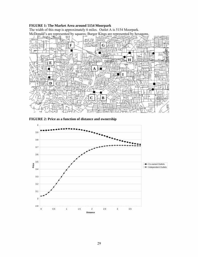
FIGURE 1: The Market Area around 5154 Moorpark The width of this map is approximately 6 miles. Outlet A is 5154 Moorpark. McDonald’s are represented by squares; Burger Kings are represented by hexagons.

F G

HE

AI

D

C B

FIGURE 2: Price as a function of distance and ownership

2.9

3

3.1

3.2

3.3

3.4

3.5

3.6

3.7

3.8

3.9

4

0 0.5 1 1.5 2 2.5 3 3.5

Distance

Pric

e Co-owned OutletsIndependent Outlets

29

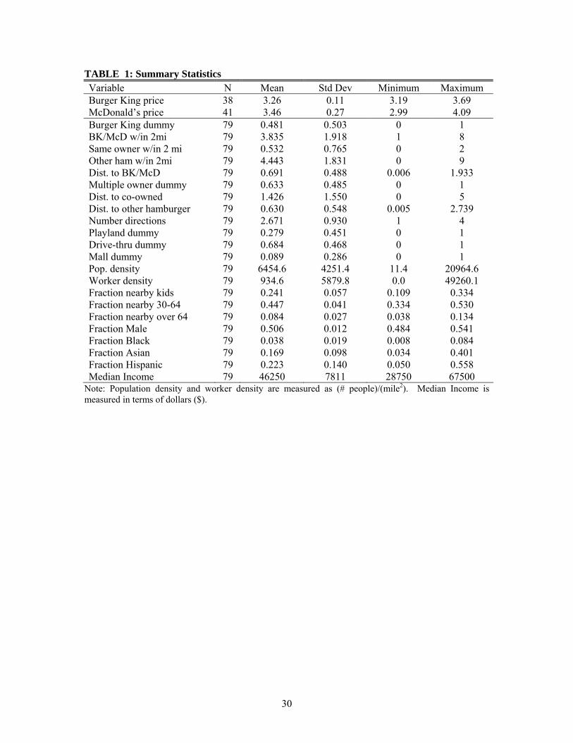
TABLE 1: Summary Statistics Variable N Mean Std Dev Minimum Maximum Burger King price 38 3.26 0.11 3.19 3.69 McDonald’s price 41 3.46 0.27 2.99 4.09 Burger King dummy 79 0.481 0.503 0 1 BK/McD w/in 2mi 79 3.835 1.918 1 8 Same owner w/in 2 mi 79 0.532 0.765 0 2 Other ham w/in 2mi 79 4.443 1.831 0 9 Dist. to BK/McD 79 0.691 0.488 0.006 1.933 Multiple owner dummy 79 0.633 0.485 0 1 Dist. to co-owned 79 1.426 1.550 0 5 Dist. to other hamburger 79 0.630 0.548 0.005 2.739 Number directions 79 2.671 0.930 1 4 Playland dummy 79 0.279 0.451 0 1 Drive-thru dummy 79 0.684 0.468 0 1 Mall dummy 79 0.089 0.286 0 1 Pop. density 79 6454.6 4251.4 11.4 20964.6 Worker density 79 934.6 5879.8 0.0 49260.1 Fraction nearby kids 79 0.241 0.057 0.109 0.334 Fraction nearby 30-64 79 0.447 0.041 0.334 0.530 Fraction nearby over 64 79 0.084 0.027 0.038 0.134 Fraction Male 79 0.506 0.012 0.484 0.541 Fraction Black 79 0.038 0.019 0.008 0.084 Fraction Asian 79 0.169 0.098 0.034 0.401 Fraction Hispanic 79 0.223 0.140 0.050 0.558 Median Income 79 46250 7811 28750 67500

Note: Population density and worker density are measured as (# people)/(mile2). Median Income is measured in terms of dollars ($).

30

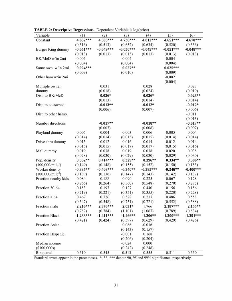
TABLE 2: Descriptive Regressions. Dependent Variable is log(price) Variable (1) (2) (3) (4) (5) (6) Constant 4.632*** 4.503*** 4.736*** 4.812*** 4.651*** 4.670*** (0.516) (0.513) (0.652) (0.634) (0.520) (0.556) Burger King dummy -0.051*** -0.049*** -0.050*** -0.049*** -0.051*** -0.048*** (0.013) (0.013) (0.013) (0.013) (0.013) (0.013) BK/McD w/in 2mi -0.005 -0.004 -0.004 (0.004) (0.004) (0.004) Same own. w/in 2mi 0.024*** 0.027** 0.025*** (0.009) (0.010) (0.009) Other ham w/in 2mi -0.002 (0.004) Multiple owner 0.031 0.028 0.027 dummy (0.018) (0.024) (0.019) Dist. to BK/McD 0.026* 0.026* 0.028** (0.013) (0.014) (0.014) Dist. to co-owned -0.013** -0.012* -0.012* (0.006) (0.007) (0.006) Dist. to other hamb. -0.011 (0.013) Number directions -0.017** -0.018** -0.017** (0.007) (0.008) (0.007) Playland dummy -0.005 0.004 -0.003 0.006 -0.005 0.004 (0.014) (0.014) (0.015) (0.015) (0.014) (0.014) Drive-thru dummy -0.013 -0.012 -0.016 -0.014 -0.012 -0.014 (0.015) (0.015) (0.017) (0.017) (0.015) (0.016) Mall dummy 0.019 0.038 0.019 0.038 0.020 0.038 (0.028) (0.030) (0.029) (0.030) (0.029) (0.030) Pop. density 0.332** 0.414*** 0.329** 0.396** 0.334** 0.386** (100,000/mile2) (0.149) (0.148) (0.155) (0.152) (0.150) (0.153) Worker density -0.335** -0.408*** -0.340** -0.385*** -0.346** -0.400*** (100,000/mile2) (0.139) (0.136) (0.147) (0.143) (0.142) (0.137) Fraction nearby kids 0.084 0.188 0.090 -0.225 0.067 0.128 (0.266) (0.264) (0.560) (0.548) (0.270) (0.275) Fraction 30-64 0.153 0.197 0.127 0.440 0.156 0.156 (0.219) (0.221) (0.351) (0.355) (0.220) (0.228) Fraction > 64 0.467 0.726 0.528 0.217 0.486 0.558 (0.547) (0.548) (0.751) (0.721) (0.552) (0.588) Fraction male 2.216*** 2.376*** 2.031* 1.766 2.187*** 2.155** (0.782) (0.784) (1.101) (1.067) (0.789) (0.834) Fraction Black -1.233*** -1.411*** -1.466** -1.306** -1.200*** -1.391*** (0.421) (0.424) (0.597) (0.629) (0.429) (0.426) Fraction Asian 0.086 -0.016 (0.143) (0.157) Fraction Hispanic -0.001 0.168 (0.206) (0.204) Median income -0.024 0.000 ($100,000s) (0.242) (0.248) R-squared 0.510 0.545 0.513 0.555 0.511 0.550

Standard errors appear in the parentheses. *, **, *** denote 90, 95 and 99% significance, respectively.

31

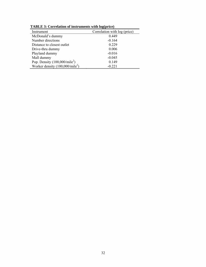
TABLE 3: Correlation of instruments with log(price) Instrument Correlation with log (price) McDonald’s dummy 0.449 Number directions -0.164 Distance to closest outlet 0.229 Drive-thru dummy 0.006 Playland dummy -0.016 Mall dummy -0.045 Pop. Density (100,000/mile2) 0.149 Worker density (100,000/mile2) -0.221

32

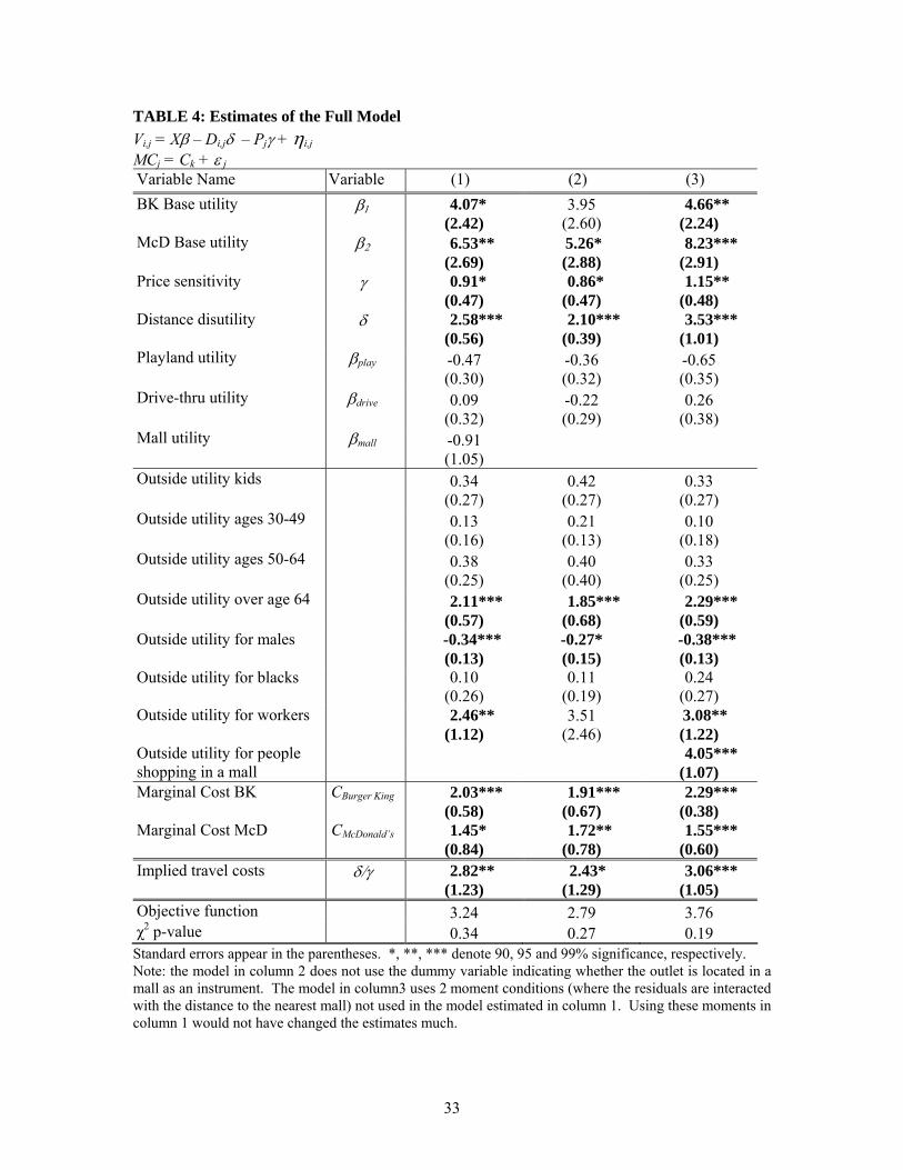
TABLE 4: Estimates of the Full Model Vi,j = Xβ – Di,jδ – Pjγ + ηi,j

MCj = Ck + ε j

Variable Name Variable (1) (2) (3) BK Base utility β1 4.07*

(2.42) 3.95

(2.60) 4.66**

(2.24) McD Base utility β2 6.53**

(2.69) 5.26* (2.88)

8.23*** (2.91)

Price sensitivity γ 0.91* (0.47)

0.86* (0.47)

1.15** (0.48)

Distance disutility δ 2.58*** (0.56)

2.10*** (0.39)

3.53*** (1.01)

Playland utility βplay -0.47 (0.30)

-0.36 (0.32)

-0.65 (0.35)

Drive-thru utility βdrive 0.09 (0.32)

-0.22 (0.29)

0.26 (0.38)

Mall utility βmall -0.91 (1.05)

Outside utility kids 0.34 (0.27)

0.42 (0.27)

0.33 (0.27)

Outside utility ages 30-49 0.13 (0.16)

0.21 (0.13)

0.10 (0.18)

Outside utility ages 50-64 0.38 (0.25)

0.40 (0.40)

0.33 (0.25)

Outside utility over age 64 2.11*** (0.57)

1.85*** (0.68)

2.29*** (0.59)

Outside utility for males -0.34*** (0.13)

-0.27* (0.15)

-0.38*** (0.13)

Outside utility for blacks 0.10 (0.26)

0.11 (0.19)

0.24 (0.27)

Outside utility for workers 2.46** (1.12)

3.51 (2.46)

3.08** (1.22)

Outside utility for people shopping in a mall

4.05*** (1.07)

Marginal Cost BK CBurger King 2.03*** (0.58)

1.91*** (0.67)

2.29*** (0.38)

Marginal Cost McD CMcDonald’s 1.45* (0.84)

1.72** (0.78)

1.55*** (0.60)

Implied travel costs δ/γ 2.82** (1.23)

2.43* (1.29)

3.06*** (1.05)

Objective function 3.24 2.79 3.76 χ2 p-value 0.34 0.27 0.19

Standard errors appear in the parentheses. *, **, *** denote 90, 95 and 99% significance, respectively. Note: the model in column 2 does not use the dummy variable indicating whether the outlet is located in a mall as an instrument. The model in column3 uses 2 moment conditions (where the residuals are interacted with the distance to the nearest mall) not used in the model estimated in column 1. Using these moments in column 1 would not have changed the estimates much.

33

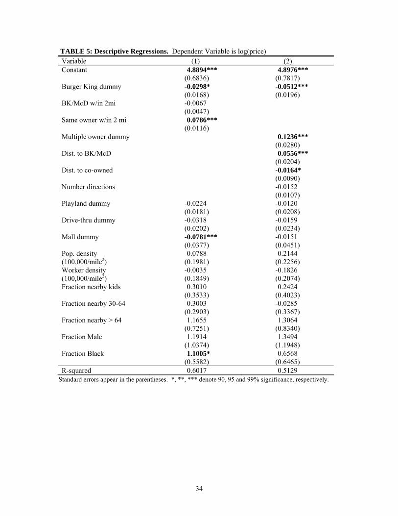
TABLE 5: Descriptive Regressions. Dependent Variable is log(price) Variable (1) (2) Constant 4.8894*** 4.8976*** (0.6836) (0.7817) Burger King dummy -0.0298* -0.0512*** (0.0168) (0.0196) BK/McD w/in 2mi -0.0067 (0.0047) Same owner w/in 2 mi 0.0786*** (0.0116) Multiple owner dummy 0.1236*** (0.0280) Dist. to BK/McD 0.0556*** (0.0204) Dist. to co-owned -0.0164* (0.0090) Number directions -0.0152 (0.0107) Playland dummy -0.0224 -0.0120 (0.0181) (0.0208) Drive-thru dummy -0.0318 -0.0159 (0.0202) (0.0234) Mall dummy -0.0781*** -0.0151 (0.0377) (0.0451) Pop. density 0.0788 0.2144 (100,000/mile2) (0.1981) (0.2256) Worker density -0.0035 -0.1826 (100,000/mile2) (0.1849) (0.2074) Fraction nearby kids 0.3010 0.2424 (0.3533) (0.4023) Fraction nearby 30-64 0.3003 -0.0285 (0.2903) (0.3367) Fraction nearby > 64 1.1655 1.3064 (0.7251) (0.8340) Fraction Male 1.1914 1.3494 (1.0374) (1.1948) Fraction Black 1.1005* 0.6568 (0.5582) (0.6465) R-squared 0.6017 0.5129

Standard errors appear in the parentheses. *, **, *** denote 90, 95 and 99% significance, respectively.

34

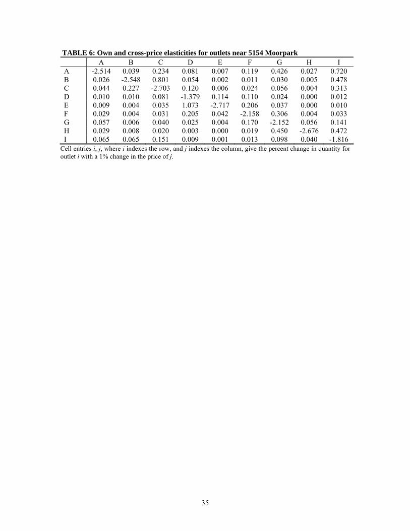
TABLE 6: Own and cross-price elasticities for outlets near 5154 Moorpark A B C D E F G H I A -2.514 0.039 0.234 0.081 0.007 0.119 0.426 0.027 0.720 B 0.026 -2.548 0.801 0.054 0.002 0.011 0.030 0.005 0.478 C 0.044 0.227 -2.703 0.120 0.006 0.024 0.056 0.004 0.313 D 0.010 0.010 0.081 -1.379 0.114 0.110 0.024 0.000 0.012 E 0.009 0.004 0.035 1.073 -2.717 0.206 0.037 0.000 0.010 F 0.029 0.004 0.031 0.205 0.042 -2.158 0.306 0.004 0.033 G 0.057 0.006 0.040 0.025 0.004 0.170 -2.152 0.056 0.141 H 0.029 0.008 0.020 0.003 0.000 0.019 0.450 -2.676 0.472 I 0.065 0.065 0.151 0.009 0.001 0.013 0.098 0.040 -1.816

Cell entries i, j, where i indexes the row, and j indexes the column, give the percent change in quantity for outlet i with a 1% change in the price of j.

35

Endnotes: 1 I wish to thank my advisors Frank Wolak, B. Douglas Bernheim and Peter Reiss for their guidance and support, Aviv Nevo who gave me extensive comments on this paper, and Ariel Pakes and two anonymous referees. Chonira Aturupane, Pat Bayer, Stan Black, Dina and Ron Borzekowski, Kevin Davis, Tracy Falba, Elizabeth Goldstein, Ali Hortacsu, Philippe Leupin, Kristin Madison, Dina Older-Aguilar, Jon Rork, Akila Weerapana and Pai Yin helped collect the data and gave many useful comments. I also benefited from discussions with Pat Bajari, Steve Berry, Peter Davis, Tom Hubbard, Jun Ishii, Francine Lafontaine, Koshy Mathai, Cristian Santestaban and seminar participants at several seminars. Email: rct27@columbia.edu. 2 While many companies keep the data as proprietary information, more and more individual-choice data including the outlet from which goods are purchased is available from sources such as AC Nielsen. However, this data can be very expensive, tends to be oriented towards home consumable products, and does not exist for many industries, especially service industries such as hair salons, ice cream parlors, ATMs, legal or medical services, and recreational activities (such as golf courses), for example. 3 This figure is the national daily average number of customers who eat in each McDonald’s (1540 per day according to McDonald’s corporation), times the number of McDonald’s in Santa Clara County, divided by the population of the county. Another 3.5% go to a Burger King on any given day. 4 About 65% of McDonald’s and 92% of Burger Kings in the US are franchised. (2002 McDonald’s Annual Report, Burger King Corporate facts at http://www.burgerking.com/ on December 19, 2003.) Note the figure for McDonald’s contrasts with their figure of 85% as cited in footnote 12. 5 See Love (1995), for example. 6 See Love (1995) and Shook and Shook (1993). 7 See McLamore (1997). 8 See Shook and Shook (1993) and Schlosser (2002). The only exception was that Kroc had franchisees buy Multimixers from him. It was Kroc’s job as a Multimixer salesman that led him to the McDonald brothers’ store and got him involved in fast food. Multimixers are no longer used at McDonald’s outlets. 9 See Dicke (1992) and Love (1995). 10 See Love (1995). 11 See Blair and Esquibel (1996) and Lafontaine (1999). 12 The evidence of this includes the price variation I find at these outlets, the lack of academic or rumored trade discussion that price maintenance was re-imposed in the fast food industry, a conversation I had with a Burger King franchisee in 2000 who stated that Burger King did not try to set prices at the franchised outlets, and a statement on McDonald’s website stating that the franchisees could set their own prices. This last statement appears as an FAQ at http://www.mcdonalds.com/corporate/info/faq/index.html, September 6, 1999: “Why do your prices vary from one restaurant to another and why do some restaurants charge for extra condiments?” The answer: “Approximately 85 percent of McDonald's restaurants are locally owned and operated. As independent businesspeople, each individual determines his or her own prices taking their operating costs and the company's recommendations into consideration. Therefore, prices do vary from one McDonald's restaurant to another. Also, for this same reason, charges for condiments may vary from McDonald's restaurant to another.” 13 With only 4 exceptions, all Burger King and McDonald’s prices were collected between June 22 and July 29, 1999. There were no observed price changes during the period I collected prices except for specials, and these were not on items I use for the prices. 14 I obtained the locations of the outlets from the Santa Clara Department of Environmental Health, online yellow pages, and each chain’s website. I confirmed the accuracy of the locations and collected data indicating whether a drive-thru or playland was present and the full menu of prices by physically visiting the restaurants. The menu was collected through photography where possible; complete menus were written down by hand where photographs could not be taken. 15 There are no Burger King outlets in this market that are not franchised. 16 One McDonald’s and one Burger King – each in different terminals. 17 Numerous references state that these sandwiches are the chains’ best sellers, but I could not find the exact sales figures. Burger King’s website (April 5, 2001) states that Burger King sells 4-4.6 million whoppers a day to 15 million customers, implying that over ¼ of Burger King customers eat a whopper. Love (1995) reports that by 1969 the Big Mac accounted for 19% of all McDonald’s sales. McDonald’s says that their best seller is the Big Mac at http://www.mcdonalds.com/countries/usa/corporate/info/studentkit/index.html.

36

18 The unweighted average correlation between the Whopper Meal price and the other value meals is 0.54; the average correlation between the Big Mac Meal and the other extra value meals is 0.74. The unweighted average correlation across all menu items is 0.51 and 0.55, respectively. 19 Using a cutoff of 1.5 miles gives similar results, with larger standard errors on the competitive variables. 20 The coefficient on playland is positive in other regressions in Table 2, the coefficient on drive-thru is positive when I estimate the model in Section 3 21 = I(1 or more firms within 2 miles NW of the outlet) + I(1 or more firms within 2 miles SW of the outlet) + I(1 or more firms within 2 miles SE of the outlet) + I(1 or more firms within 2 miles NE of the outlet). 22 If other hamburger outlets were competitors then prices should increase as these competitors are further away. Instead the coefficient is negative. 23 See Ashenfelter, et al. (2004) and Reiss and Wolak (2004) for more discussion of these issues. 24 I assume that consumers are perfectly informed about the prices, locations and food quality at all outlets. 25 Quantity data can come in a micro format or an aggregate format, where BLP-style methods are used. 26 An exception is the automobile industry, the focus of BLP, where obtaining transaction prices is difficult. 27 Davis (2001) and Manuszak (2000) both use similar frameworks. 28 Distances are measured as the shortest route along existing streets, except for distances to malls which are calculated using Euclidean distances due to inaccuracies in the official road patterns that exist around malls. 29 While there could theoretically be some unobserved heterogeneity in the quality of different outlets – for example, some restaurants could be cleaner than others – I did not observe many differences in my personal visits to these outlets in my study area. In contrast with many other urban markets, I found that all but one of the McDonald’s and Burger King restaurants that I visited in the county appeared to be very clean. 30 Because the county is largely surrounded by mountains or a bay, only two of the outlets whose price-setting behavior I use are located within one mile of the county border. I ignore the demand and competition effects from neighboring counties. However, the market conditions are similar on both sides of the border. 31 See pp. 118-122 of Reiter (1991) or pp. 73-74 of Schlosser (2001). 32 Including fixed costs for the total joint operation of several outlets would not affect my estimation. 33 I assume that these unobserved costs are uncorrelated across outlets among owners. To support this, I calculated the correlation between the fitted residual for each outlet and the mean of these fitted residuals across all of the other outlets owned by the same owner. The correlation is -0.15. All but two owners have at least one outlet with negative and one outlet with positive unobservable components of marginal costs, and the two exceptions only own two and three outlets, respectively. 34 Part of the residual may also come from different franchise rates that the different franchisees have to pay. This will not prove to be problematic, since, as described in Section 2.1, the franchise rate varies only with the date that the contract was signed, and not with the location of the outlet. 35 Reiter (1991), pp. 103-104, 116-126; Schlosser (2001), pp. 74-75, 82-83; Emerson (1990), pp. 102-104. 36 These shift demand, too, but the other instruments I use are demand shifters. 37 A firm that is further from its nearest competitor has higher demand, all else equal, and is able to charge a higher price. A similar argument applies to the number of directions of competing outlets, which is described in section 2.3. Changing the 2 mile cutoff to 1.5 miles does not change the estimates much. 38 Note that this is similar to the assumption in BLP that the non-price attributes of outlets and those of their competitors are uncorrelated with the outlet’s unobserved component of marginal cost. This assumption is consistent with the findings of Toivanen and Waterson (2001), who use panel data to conclude that unobservable location attributes do not play an important role in fast food decisions. See, too, Sault, Toivanen and Waterson (2002) for more on entry in the fast food industry. 39 See p. 104 Emerson (1990), p. 104 of Reiter (1991) and p. 74 of Schlosser (2001). 40 While absolute population densities of consumers are unimportant, relative densities are important. Higher absolute densities of the nearest block-group are correlated with higher probabilities that the density of consumers near the firm is higher than the density a little further away. 41 The correlation between worker density and population density is -0.14. 42 That is, E[Zjε j(θ*)] = 0 still holds. 43 See Chapter 3 of Thomadsen (2001) for more on this. 44 Note that there is a parallel between (i) the requirement that the rate of change in the markup term as a function of market geography be unique in the demand parameters and (ii) the result in Bresnahan (1982)

37

that it is important that the markup term be unique in the level of market power variable in order to identify the oligopoly solution concept. 45 In this final model, the number of consumers that are located at each mall is determined by regressing the number of daily shoppers at the three malls in the county that report the number of people who come to the mall on a constant and the number of square feet in the mall, and then using these estimates and the size of each mall to get the fitted number of customers. For daily customers, I take the number of weekly shoppers (as reported by the Directory of Major Malls (2000)) and divide by seven. The three malls are Oakridge, Valley Fair and the Great Mall of Milpitas. The regression yields that the number of customers = – 20461 + 0.0458 x area of mall. The standard errors of the point estimates are 5238 and 0.0048, respectively. 46 Note that a person going to an outlet 1 mile away travels 2 miles round trip. It takes approximately 3 minutes to travel 1 mile in my study area. Subtracting the 1999 US GSA’s 31-cent per mile deduction as true costs (see http://www.gsa.gov/Portal/gsa/ep/contentView.do?contentId=9646&contentType=GSA_BASIC) yields an hourly cost of the time of $27/hour. (Greg Rosston pointed this out.) Wages in Silicon Valley were high at the time: median income was $59,639 (http://quickfacts.census.gov/qfd/states/06/06085.html). Note that two opposing effects make it difficult to compare travel costs to annual income. On one hand, money spent on fast food comes from post-tax income, implying that travel costs should be lower than the median salary. However, the opportunity cost of time away from work is higher than that of time at work since the marginal opportunity cost of leisure grows as there are fewer and fewer of these hours left. This intuition is codified in the requirement that US employers pay employees time and a half for overtime hours. 47 Defined as price above marginal cost. See Tirole (1995), p.284 for different definitions of market power. 48 The estimates reported in Table 4 are for the true marginal cost divided by the fraction of the revenue that the franchisee keeps, as shown in equation (7). I use the current effective franchise rates as reported on each chain’s website on July 21, 2004. BK franchisees keep 91.5% of their revenues according to http://www.burgerking.com/CompanyInfo/FranchiseOpps/us/franchisee_facts.aspx. McD’s franchisees keep 87.5% of their revenues (http://www.mcdonalds.com/corp/franchise/mrktspecific/usa/fact_sheet.html). 49 Fast food firms often posted ads/signs with starting wages above $8/hour – well above minimum wage. 50 Equals actual prices minus the residual from each outlet’s idiosyncratic cost variation. 51 Compare columns B and C for an illustration of this. 52 The owner of 5925 Almaden owns two other outlets, both of which are so far away that their existence does not affect the price at 5925 Almaden. The owner of the Oakridge mall outlet owns 2 other outlets. 53 And all of the other outlets owned by this outlet’s owner. 54 Perloff et al (1996) demonstrate that entry can cause prices to increase in differentiated industries. Thomadsen (2004) demonstrates that this can happen with this estimated model, although the price increases are pretty minimal in the few cases where entry actually increases prices. 55 Practically, this involves swapping both the base utility of the chain and the mean marginal cost of the chain, so now McDonald’s base utility is 4.07 and Burger King’s base utility is 6.53. Similarly, McDonald’s mean marginal cost is now $2.03 and Burger King’s mean marginal cost is now $1.45. 56 For the purposes of this statement, the firm that is the market leader is the firm with the highest value of Xjβ – Cjγ, where Cj is the marginal cost of the product.

38