trend and linearity analysis of meteorological parameters in

Sustainability 2020, 12, 9533; doi:10.3390/su12229533 www.mdpi.com/journal/sustainability

Article

Trend and Linearity Analysis of Meteorological

Parameters in Peninsular Malaysia

Farahani Mohd Saimi 1, Firdaus Mohamad Hamzah 1,*, Mohd Ekhwan Toriman 2,*, Othman Jaafar 1

and Hazrina Tajudin 1

1 Faculty of Engineering and Build Environment, National University of Malaysia, Bangi 43600, Malaysia;

[email protected] (F.M.S.); [email protected] (O.J.); [email protected] (H.T.) 2 Faculty of Social Sciences and Humanities, National University of Malaysia, Bangi 43600, Malaysia

* Correspondence: [email protected] (F.M.H.); [email protected] (M.E.T.); Tel.: +603−93488786 (F.M.H.);

Tel.: +603-89213648 (M.E.T.)

Received: 9 August 2020; Accepted: 25 October 2020; Published: 16 November 2020

Abstract: Climate change has often led to severe impact on the environment. This study aimed to

investigate the monthly trends and linearity of meteorological parameters at four locations during

the period from 1970 to 2016. These locations represent the south, north, east, and west of Peninsular

Malaysia. The meteorological parameters used were monthly total precipitation (mm) and monthly

average temperature (°C). To illustrate the methodology, the Mann–Kendall (MK) trend test and a

non-parametric regression model were used. The MK trend test did not indicate significant trends in

precipitation, but indicated a trend in temperature for all locations. The Sen value gives the amount

of fluctuation of precipitation and temperature for every year. The results of the linearity test

exhibited a linear trend for precipitation and temperature for most of the months throughout the

study period. Thus, this study gives insights into the monthly trends of meteorological parameters,

especially in Peninsular Malaysia.

Keywords: Mann–Kendall trend test; non-parametric regression; Sen slope; linearity test;

meteorological parameter

1. Introduction

Hydrological patterns may be unpredictable due to their responses to changes in precipitation,

temperature, and other meteorological parameters [1]. Previous studies reported that extreme

weather events can cause loss of life and tremendous economic losses [2,3]. An increasing number of

hydrological studies in Malaysia have been carried out over the past several decades in order to

provide better knowledge about our climate. The climate in Peninsular Malaysia is affected by two

monsoons and two inter-monsoon seasons. The Southwest Monsoon (SWM) lasts from May until

September and the Northeast Monsoon (NEM) lasts from November until March, while the

inter-monsoon (IM) seasons are in April and October [4]. The SWM is the driest season in all states in

Malaysia, with the exception of Sabah in East Malaysia. Most states receive the lowest amount of

rainfall during this season. In contrast, the NEM is the wettest season for most states in Malaysia.

This monsoon season is characterized by severe flooding events, especially in the east coast states of

Kelantan, Terengganu, Pahang, and east Johor in Peninsular Malaysia, as well as in Sarawak [5]. In

light of this, analysis of meteorological parameters has become one of the most important

assessment tools in studying and understanding the patterns of climate change in this country.

The change in meteorological patterns experienced by each country is unique; for instance,

precipitation is influenced by several factors, including topography, temperature, and wind [6]. As a

result, climate change projections related to high temperature events are becoming increasingly

Sustainability 2020, 12, 9533 2 of 19

important due to their impact on the well-being of populations and ecosystems [7]. A previous study

in Mozambique showed that renewable energy, such as hydropower and biomass, is the most

affected by climate change. The fluctuation of hydrological parameters, such as temperature and

precipitation, can affect the energy generated from these renewable resources [8]. According to the

Malaysian Meteorological Department [9], among the apparent effects of climate change is the

increase in annual temperature by 0.02 °C in Peninsular Malaysia, which is equivalent to 2 °C per 100

years. In their study, Hansen [9] stated that the global surface temperature has increased by 0.2 °C

per decade in the last 30 years, similar to the warming rate predicted in the 1980s in initial global

climate model simulations. Temperature has a considerable influence on climate change, and

increases in temperature will increase the risk of occurrence of several diseases [10,11]. The National

Hydraulic Research Institute of Malaysia (NAHRIM) reported a 17% increase in the amount of

rainfall since 2000 compared with the amount recorded in 1970 [12].

The observed temperature and precipitation trends in the twentieth century suggest that the

country’s climate is changing, and these changes include a long-term warming trend interspersed

with more frequent high temperature events and an increase in the volume of precipitation [13].

Akhtar [14] showed that a trend of increasing annual temperature will lead to a decrease in average

annual rainfall. The findings of previous studies have provided some important insights into the

effects of climate change in Malaysia.

Many scientific works have explored the trends in hydrometeorological time series [15], and trend

identification has become an important factor in hydrological time series analysis [16]. Malaysia has

experienced warming and rainfall irregularities, particularly in the last two decades. Thus, it is garnering

much attention in the study of climate trends and their implications [17]. Therefore, investigating the

mean monthly trends and linearity of meteorological parameters in Peninsular Malaysia will be the main

objective of this study. Following that, the results obtained from each station are compared.

2. Study Area and Data

2.1. Data

The meteorological data used were a monthly time series spanning 47 years from 1970 to 2016

for all parameters. The parameters involved were monthly average precipitation (mm) and

temperature (°C). These meteorological parameters were available for all meteorological stations,

and the data were provided by the Malaysian Meteorological Department (MMD). The data were

sorted by month, and the time series data were recorded as a homogenized time series dataset.

Homogenizing a dataset is a process that assembles all the data collected at specific sites and

times with particular instruments under a set of standard procedures [18] to ensure consistency of

data, integrity of analysis, and validity of results [19]. The factors that frequently influence the

non-homogenous datasets are monitoring station relocation, changes in instrumentation, changes in

the surroundings, instrumental inaccuracies, and changes in observational and calculation

procedures [20]. In order to avoid having non-homogenized datasets, meteorological stations have

developed their own procedures to identify and remove all of the factors that influence

non-homogenized datasets. Using a non-homogenized dataset, especially for climate data, will

potentially bias the result. Meteorological stations (airports) have their own measurement standards

for data collection to meet their desired standards.

2.2. Study Area

The four (4) meteorological stations in Peninsular Malaysia chosen for this study are Senai

International Airport (South, 37.8 m above sea level, 01°38′ N,03°40′ E: Senai), Alor Setar Airport

(North, 3.9 m above sea level, 06°12′ N,100°24′ E: Alor Setar), Sultan Ahmad Shah Airport (East,

15.23 m above sea level, 03°47′ N, 103°13′ E: Kuantan), and Sultan Abdul Aziz Shah Airport (West,

16.64 m above sea level, 03°06′ N,101°39′ E: Subang). All four selected stations were chosen due to

their location, where the Alor Setar Airport, Senai International Airport, Sultan Ahmad Shah Airport


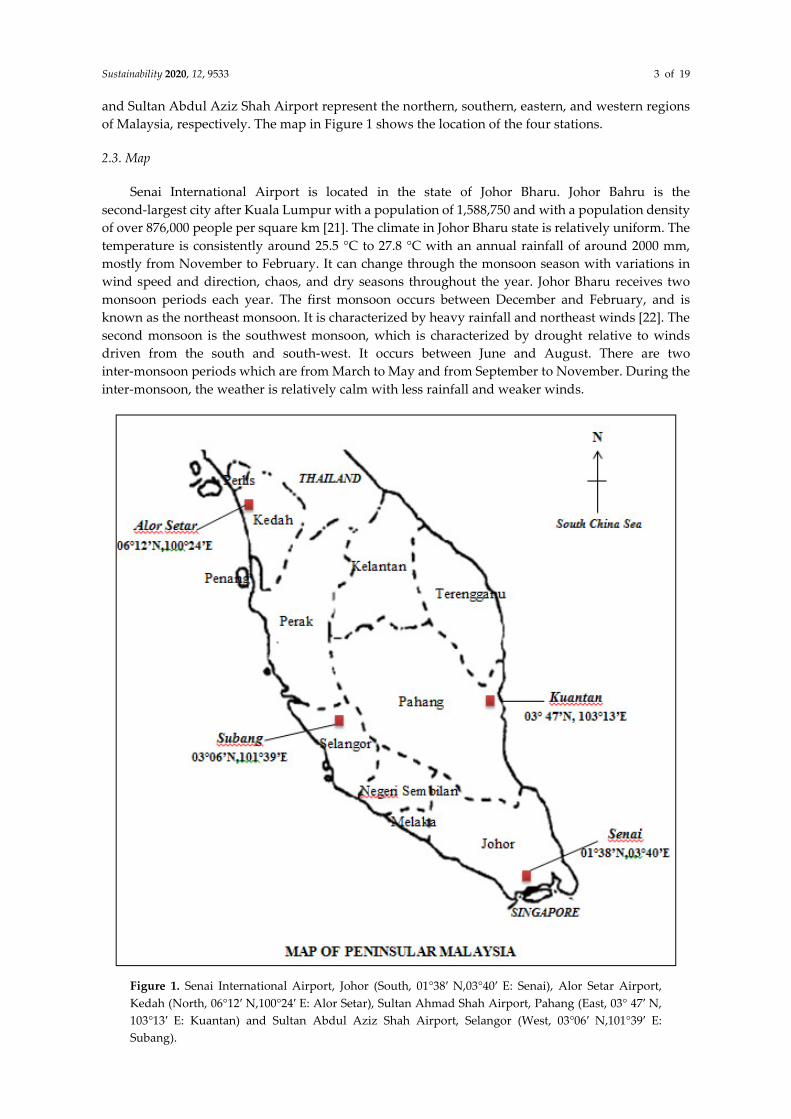
and Sultan Abdul Aziz Shah Airport represent the northern, southern, eastern, and western regions

of Malaysia, respectively. The map in Figure 1 shows the location of the four stations.

2.3. Map

Senai International Airport is located in the state of Johor Bharu. Johor Bahru is the

second-largest city after Kuala Lumpur with a population of 1,588,750 and with a population density

of over 876,000 people per square km [21]. The climate in Johor Bharu state is relatively uniform. The

temperature is consistently around 25.5 °C to 27.8 °C with an annual rainfall of around 2000 mm,

mostly from November to February. It can change through the monsoon season with variations in

wind speed and direction, chaos, and dry seasons throughout the year. Johor Bharu receives two

monsoon periods each year. The first monsoon occurs between December and February, and is

known as the northeast monsoon. It is characterized by heavy rainfall and northeast winds [22]. The

second monsoon is the southwest monsoon, which is characterized by drought relative to winds

driven from the south and south-west. It occurs between June and August. There are two

inter-monsoon periods which are from March to May and from September to November. During the

inter-monsoon, the weather is relatively calm with less rainfall and weaker winds.

Figure 1. Senai International Airport, Johor (South, 01°38′ N,03°40′ E: Senai), Alor Setar Airport,

Kedah (North, 06°12′ N,100°24′ E: Alor Setar), Sultan Ahmad Shah Airport, Pahang (East, 03° 47′ N,

103°13′ E: Kuantan) and Sultan Abdul Aziz Shah Airport, Selangor (West, 03°06′ N,101°39′ E:

Subang).


Alor Setar Airport is located in the state of Kedah, which is located in the district of Kota Setar.

Kedah is bordered by three states and one country, namely Perlis (Northwest), Penang (Southwest),

Perak (South), and Thailand (North). The climate in Alor Setar is hot and overcast. Over the year, the

temperature typically varies from 23 °C to 33 °C, and rarely below 21 °C or above 35 °C. Alor Setar

experiences seasonal variation in monthly rainfall. The amount of rainfall in Alor Setar is according to

season and time. The least rainfall is expected in January and February with an average of 80 mm. This

condition is due to the very dry weather conditions. The high density of rainfall starts from March to

October ranging between around 110 mm and 160 mm. November records the highest amount of

rainfall ranging between 150 mm and 250 mm. Currently, thunderstorms accompanied by heavy

rainfall occur frequently in the afternoon, and the amount of rainfall began to decrease to less than 150

mm starting in December.

Kuantan Airport, also known as The Sultan Ahmad Shah Airport, is located in the state of

Kuantan, Pahang. The climate features a tropical rainforest climate where it experiences a dry and hot

season and a rainy season. The dry and hot season occurs when seasonal winds from southwest

Sumatra, Indonesia, blow and move towards the west coast of Peninsular Malaysia, and are blocked

by the Titiwangsa Mountain Range. The temperature can reach 40 °C. However, the temperature

mostly varies from 23 °C to 32 °C. Kuantan is a city with significant rainfall. The heavy rain season is

between October and March, and is caused by winds from the north. Even during the driest month,

Kuantan still receives a large amount of rainfall, with the annual amount reported to be around 2800

mm.

Sultan Abdul Aziz Shah Airport, also known as Subang Airport, is located in the state of

Selangor. Subang is located at a high altitude, 28 m above sea level and has a high temperature with a

minimum annual temperature of 27.7 °C [23]. The temperature is rarely below 23 °C or above 34 °C.

The rainfall here is around 2360 mm per year [24]. Subang has the highest number of days with

lightning. It was recorded as 362 days in 1987. The climate in Subang is a tropical climate and has a

significant amount of rainfall during the year. A lot of rain falls in the months of January, March, April,

May, September, and from October to December. April is the wettest month in Subang Jaya, where

rainfall can last from around 10 to 14 days, whereas June is the driest, with precipitation occurring

from around seven to nine days.

3. Methods

Non-parametric statistical methods have been employed to analyze the linearity and temporal

trends of meteorological parameters. R programming is used as a tool to carry out and run the

analysis for both methods [25–27].

3.1. Mann–Kendall Trend Test

The Mann–Kendall (MK) trend test was used to identify the presence of a monotonic trend in

each meteorological parameter. The primary reason for using the non-parametric statistical tests is

that they are more appropriate for abnormal data distribution. Additionally, the Mann–Kendall

trend test is a frequently employed statistical test for analyzing climate trend variables [28,29] and

also in the analysis of time series [30,31]. The non-parametric Mann–Kendall statistical method is the

primary method utilized in the present study since it is very useful in hydro-meteorological studies

as it is not affected by outliers [32]. The MK statistical test is based on the test proposed by Mann [33]

and was further improved by Kendall [34].

A positive Z value indicates an increasing trend while a negative value indicates a decreasing

trend [35]. The confidence level of 95% represents a significance level of 0.5 . The null hypothesis

(no trend) is rejected for confidence above 95%.

3.2. Sen Slope Estimator Test

In addition to the MK trend test, the Sen slope estimator has also been used as an improved

method from the MK trend to identify the magnitude of change for all the climate change


parameters involved. The Sen slope estimator has been widely used in hydro-meteorological time

series [36]. Sen [37] developed the non-parametric procedure for estimating the slope of the trend

(magnitude of change) in the sample of N pairs of data. A positive value indicates an upward or

increasing trend, while a negative value indicates a downward or decreasing trend.

3.3. Non-Parametric Regression Model

The regression model is the most frequently employed statistical tool [38]. Linear modeling is

one of the most developed techniques for verifying the assumptions between predictor

(independent) variables and response (dependent) variables [39]. However, there are cases where

such models cannot be utilized due to the intrinsic nonlinearity of the data. The non-parametric

regression model is not restricted by any functional equation, which allows it to omit the linearity

assumption, thereby allowing for greater flexibility when necessary [40].

The equation for the non-parametric regression model is written as follows:

; 1,2,3....i i iy f x i n (1)

where the error i is assumed to be independently and normally distributed with mean zero and

constant variance 2 (0, )i NID . In order to omit the assumption of linearity, 0 1 ix in the

parametric trend function is replaced with a smoothing function, if x , to allow for greater

flexibility. Thus, non-parametric regression was used as it provides scatterplot smoothing to

summarize between the response variable, iy (year) and single predictor ix (precipitation or

temperature). High fluctuations in monthly precipitation data and temperature because of the strong

influence of the monsoons make it difficult to interpret the overall pattern. Smoothing the data will

help to remove the outliers and give a smooth curve, enabling the important patterns to stand out.

3.3.1. Linearity Test

Local linear regression is a non-parametric approach proposed by Cleveland [41], and is

employed to estimate the smoothing function. It is easy to use, provides benefits in certain situations

[42], and is able to reduce the bias f

in local averaging [43]. It can be adjusted to capture unusual

or unexpected features of the data. Precipitation and temperature data will probably contain

outliers, leading to difficulties in interpreting the graphical result even with a small dataset. The

result can be evaluated using a graphical approach, which is then supported by the statistical

approach.

3.3.2. Smoothing Parameter

A smoothing parameter is required to illustrate the results of the estimated smoothing. Smoothing

the data will remove the noise and help to predict different trends and patterns [44]. The smoothing of a

dataset , 1( )

n

i i ix y

involves the approximation of a mean response curve f in a regression

relationship.

; 1,2,3....i i iy f x i n

(2)

A smoothing parameter is sometimes referred to as bandwidth [45]. The degree of smoothing is

influenced by the selected smoothing parameter. The selected smoothing number is assumed to be

large to reduce the variability in a smooth point without jeopardizing the trend in the data [45]. It is

important to choose the correct smoothing parameter. Higher smoothing values produce curves that

are almost a straight line while smaller values produce a curve with greater flexibility [46].

Several methods can be used to select a smoothing parameter, such as Cross Validation (CV)

[47], Generalized Cross Validation (GCV) [48], Akaike’s Information Criterion (AIC) [49], and

Improved AIC Criterion (AICc) [50]. CV is an appropriate technique for constructing a density

estimate or regression of non-parametric curves in one or two dimensions. The basic idea of CV is to

leave the data points out one at a time and to choose the value of s that minimizes the CV score

[51]. The method of CV for choosing the smoothing parameter s from the data has been suggested


and developed by Craven [52]. The CV function is among the most popular used in local linear

regression [53]. CV is expressed as follows:

2

1

1( )

n

i si

CV s y f x in

(3)

where, n is the number of data points, iy is the i th response, and if

is the fitted value at ( )x i .

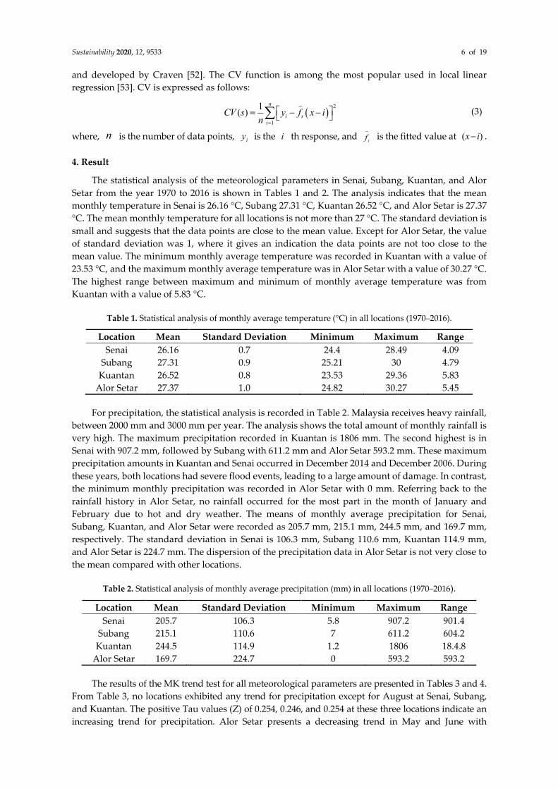
4. Result

The statistical analysis of the meteorological parameters in Senai, Subang, Kuantan, and Alor

Setar from the year 1970 to 2016 is shown in Tables 1 and 2. The analysis indicates that the mean

monthly temperature in Senai is 26.16 °C, Subang 27.31 °C, Kuantan 26.52 °C, and Alor Setar is 27.37

°C. The mean monthly temperature for all locations is not more than 27 °C. The standard deviation is

small and suggests that the data points are close to the mean value. Except for Alor Setar, the value

of standard deviation was 1, where it gives an indication the data points are not too close to the

mean value. The minimum monthly average temperature was recorded in Kuantan with a value of

23.53 °C, and the maximum monthly average temperature was in Alor Setar with a value of 30.27 °C.

The highest range between maximum and minimum of monthly average temperature was from

Kuantan with a value of 5.83 °C.

Table 1. Statistical analysis of monthly average temperature (°C) in all locations (1970–2016).

Location Mean Standard Deviation Minimum Maximum Range

Senai 26.16 0.7 24.4 28.49 4.09

Subang 27.31 0.9 25.21 30 4.79

Kuantan 26.52 0.8 23.53 29.36 5.83

Alor Setar 27.37 1.0 24.82 30.27 5.45

For precipitation, the statistical analysis is recorded in Table 2. Malaysia receives heavy rainfall,

between 2000 mm and 3000 mm per year. The analysis shows the total amount of monthly rainfall is

very high. The maximum precipitation recorded in Kuantan is 1806 mm. The second highest is in

Senai with 907.2 mm, followed by Subang with 611.2 mm and Alor Setar 593.2 mm. These maximum

precipitation amounts in Kuantan and Senai occurred in December 2014 and December 2006. During

these years, both locations had severe flood events, leading to a large amount of damage. In contrast,

the minimum monthly precipitation was recorded in Alor Setar with 0 mm. Referring back to the

rainfall history in Alor Setar, no rainfall occurred for the most part in the month of January and

February due to hot and dry weather. The means of monthly average precipitation for Senai,

Subang, Kuantan, and Alor Setar were recorded as 205.7 mm, 215.1 mm, 244.5 mm, and 169.7 mm,

respectively. The standard deviation in Senai is 106.3 mm, Subang 110.6 mm, Kuantan 114.9 mm,

and Alor Setar is 224.7 mm. The dispersion of the precipitation data in Alor Setar is not very close to

the mean compared with other locations.

Table 2. Statistical analysis of monthly average precipitation (mm) in all locations (1970–2016).

Location Mean Standard Deviation Minimum Maximum Range

Senai 205.7 106.3 5.8 907.2 901.4

Subang 215.1 110.6 7 611.2 604.2

Kuantan 244.5 114.9 1.2 1806 18.4.8

Alor Setar 169.7 224.7 0 593.2 593.2

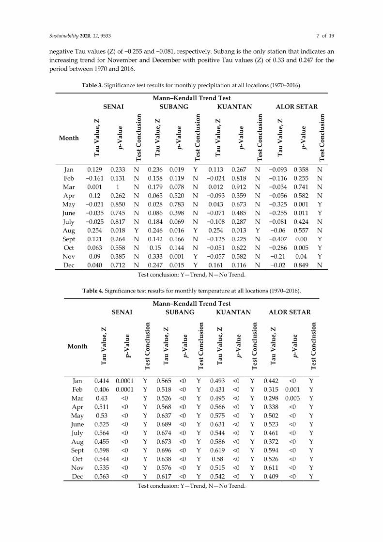
The results of the MK trend test for all meteorological parameters are presented in Tables 3 and 4.

From Table 3, no locations exhibited any trend for precipitation except for August at Senai, Subang,

and Kuantan. The positive Tau values (Z) of 0.254, 0.246, and 0.254 at these three locations indicate an

increasing trend for precipitation. Alor Setar presents a decreasing trend in May and June with


negative Tau values (Z) of −0.255 and −0.081, respectively. Subang is the only station that indicates an

increasing trend for November and December with positive Tau values (Z) of 0.33 and 0.247 for the

period between 1970 and 2016.

Table 3. Significance test results for monthly precipitation at all locations (1970–2016).

Mann–Kendall Trend Test

SENAI SUBANG KUANTAN ALOR SETAR

Month

Tau

Va

lue

, Z

p-V

alu

e

Tes

t C

on

clu

sio

n

Tau

Va

lue

, Z

p-V

alu

e

Tes

t C

on

clu

sio

n

Tau

Va

lue

, Z

p-V

alu

e

Tes

t C

on

clu

sio

n

Tau

Va

lue

, Z

p-V

alu

e

Tes

t C

on

clu

sio

n

Jan 0.129 0.233 N 0.236 0.019 Y 0.113 0.267 N −0.093 0.358 N

Feb −0.161 0.131 N 0.158 0.119 N −0.024 0.818 N −0.116 0.255 N

Mar 0.001 1 N 0.179 0.078 N 0.012 0.912 N −0.034 0.741 N

Apr 0.12 0.262 N 0.065 0.520 N −0.093 0.359 N −0.056 0.582 N

May −0.021 0.850 N 0.028 0.783 N 0.043 0.673 N −0.325 0.001 Y

June −0.035 0.745 N 0.086 0.398 N −0.071 0.485 N −0.255 0.011 Y

July −0.025 0.817 N 0.184 0.069 N −0.108 0.287 N −0.081 0.424 N

Aug 0.254 0.018 Y 0.246 0.016 Y 0.254 0.013 Y −0.06 0.557 N

Sept 0.121 0.264 N 0.142 0.166 N −0.125 0.225 N −0.407 0.00 Y

Oct 0.063 0.558 N 0.15 0.144 N −0.051 0.622 N −0.286 0.005 Y

Nov 0.09 0.385 N 0.333 0.001 Y −0.057 0.582 N −0.21 0.04 Y

Dec 0.040 0.712 N 0.247 0.015 Y 0.161 0.116 N −0.02 0.849 N

Test conclusion: Y—Trend, N—No Trend.

Table 4. Significance test results for monthly temperature at all locations (1970–2016).

Mann–Kendall Trend Test


Month

Ta

u V

alu

e, Z

p-V

alu

e

Tes

t C

on

clu

sio

n

Ta

u V

alu

e, Z

p-V

alu

e

Tes

t C

on

clu

sio

n

Ta

u V

alu

e, Z

p-V

alu

e

Tes

t C

on

clu

sio

n

Ta

u V

alu

e, Z

p-V

alu

e

Tes

t C

on

clu

sio

n

Jan 0.414 0.0001 Y 0.565 <0 Y 0.493 <0 Y 0.442 <0 Y

Feb 0.406 0.0001 Y 0.518 <0 Y 0.431 <0 Y 0.315 0.001 Y

Mar 0.43 <0 Y 0.526 <0 Y 0.495 <0 Y 0.298 0.003 Y

Apr 0.511 <0 Y 0.568 <0 Y 0.566 <0 Y 0.338 <0 Y

May 0.53 <0 Y 0.637 <0 Y 0.575 <0 Y 0.502 <0 Y

June 0.525 <0 Y 0.689 <0 Y 0.631 <0 Y 0.523 <0 Y

July 0.564 <0 Y 0.674 <0 Y 0.544 <0 Y 0.461 <0 Y

Aug 0.455 <0 Y 0.673 <0 Y 0.586 <0 Y 0.372 <0 Y

Sept 0.598 <0 Y 0.696 <0 Y 0.619 <0 Y 0.594 <0 Y

Oct 0.544 <0 Y 0.638 <0 Y 0.58 <0 Y 0.526 <0 Y

Nov 0.535 <0 Y 0.576 <0 Y 0.515 <0 Y 0.611 <0 Y

Dec 0.563 <0 Y 0.617 <0 Y 0.542 <0 Y 0.409 <0 Y

Test conclusion: Y—Trend, N—No Trend.


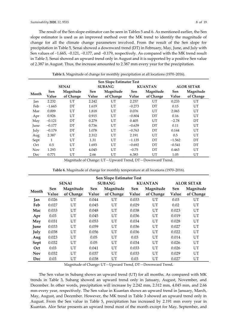
The result of the Sen slope estimator can be seen in Tables 5 and 6. As mentioned earlier, the Sen

slope estimator is used as an improved method over the MK trend to identify the magnitude of

change for all the climate change parameters involved. From the result of the Sen slope for

precipitation in Table 5, Senai showed a downward trend (DT) in February, May, June, and July with

Sen values of −1.665, −0.121, −0.177, and −0.179, respectively. As compared with the MK trend result

in Table 3, Senai showed an upward trend only in August and it is supported by a positive Sen value

of 2.387 in August. Thus, the increase amounted to 2.387 mm every year for the precipitation.

Table 5. Magnitude of change for monthly precipitation at all locations (1970–2016).

Sen Slope Estimator Test


Month Sen

Value

Magnitude

of Change

Sen

Value

Magnitude

of Change

Sen

Value

Magnitude

of Change

Sen

Value

Magnitude

of Change

Jan 2.232 UT 2.242 UT 2.257 UT 0.233 UT

Feb −1.665 DT 1.619 UT −0.273 DT 0.15 UT

Mar 0.009 UT 1.818 UT 0.076 UT 2.065 UT

Apr 0.926 UT 0.915 UT −0.804 DT 0.16 UT

May −0.121 DT 0.279 UT 0.405 UT −2.78 DT

June −0.177 DT 0.736 UT −0.639 DT 0.11 UT

July −0.179 DT 1.078 UT −0.763 DT 0.144 UT

Aug 2.387 UT 2.312 UT 2.191 UT 0.5 UT

Sept 1 UT 1.31 UT −1.135 DT −1.562 DT

Oct 0.5 UT 1.693 UT −0.692 DT −0.541 DT

Nov 1.293 UT 4.045 UT −0.75 DT 0.463 UT

Dec 0.771 UT 2.66 UT 6.383 UT 1.05 UT

Magnitude of Change: UT—Upward Trend, DT—Downward Trend.

Table 6. Magnitude of change for monthly temperature at all locations (1970–2016).

Sen Slope Estimator Test


Month Sen

Value

Magnitude

of Change

Sen

Value

Magnitude

of Change

Sen

Value

Magnitude

of Change

Sen

Value

Magnitude

of Change

Jan 0.026 UT 0.044 UT 0.033 UT 0.03 UT

Feb 0.027 UT 0.045 UT 0.029 UT 0.02 UT

Mac 0.033 UT 0.048 UT 0.038 UT 0.023 UT

Apr 0.03 UT 0.045 UT 0.036 UT 0.019 UT

May 0.031 UT 0.053 UT 0.034 UT 0.028 UT

June 0.033 UT 0.059 UT 0.036 UT 0.027 UT

July 0.038 UT 0.056 UT 0.036 UT 0.022 UT

Aug 0.023 UT 0.05 UT 0.03 UT 0.014 UT

Sept 0.032 UT 0.05 UT 0.034 UT 0.026 UT

Oct 0.03 UT 0.041 UT 0.033 UT 0.026 UT

Nov 0.032 UT 0.037 UT 0.033 UT 0.029 UT

Dec 0.03 UT 0.038 UT 0.03 UT 0.027 UT

Magnitude of Change: UT—Upward Trend, DT—Downward Trend.

The Sen value in Subang shows an upward trend (UT) for all months. As compared with MK

trends in Table 3, Subang showed an upward trend only in January, August, November, and

December. In other words, precipitation will increase by 2.242 mm, 2.312 mm, 4.045 mm, and 2.66

mm every year, respectively. The Sen value in Kuantan shows an upward trend in January, March,

May, August, and December. However, the MK trend in Table 3 showed an upward trend only in

August. From the Sen value in Table 5, precipitation has increased by 2.191 mm every year in

Kuantan. Alor Setar presents an upward trend most of the month except for May, September, and


October. The MK trend in Table 3 indicates the addition of the downward trend in June and

November. As compared with the Sen value in Table 5, precipitation decreased by −2.78 mm every

year in May, −1.562 mm in September, and −0.541 in October. Subsequently, it will increase by 0.11

mm and 0.463 every year in June and November.

Table 4 presents the result of the MK trend test of temperature at all locations. It shows a

significant value at a 95% confidence level. Temperature indicates an increasing trend during the

entire study period from 1970 to 2016. The result of the Sen slope estimator test for temperature can

be seen in Table 6, and it shows an increasing trend for all locations. The temperature increases every

year between 0.014 °C and 0.059 °C. According to the Intergovernmental Panel on Climate Change,

IPCC [54], the increasing trend was due to the 0.6 °C increase in the Earth’s average temperature in

the latter part of the 20th century. There was also a dramatic change in temperature from a minimum

of 1.4 °C to a maximum of 5.4 °C as projected by various climate prediction models.

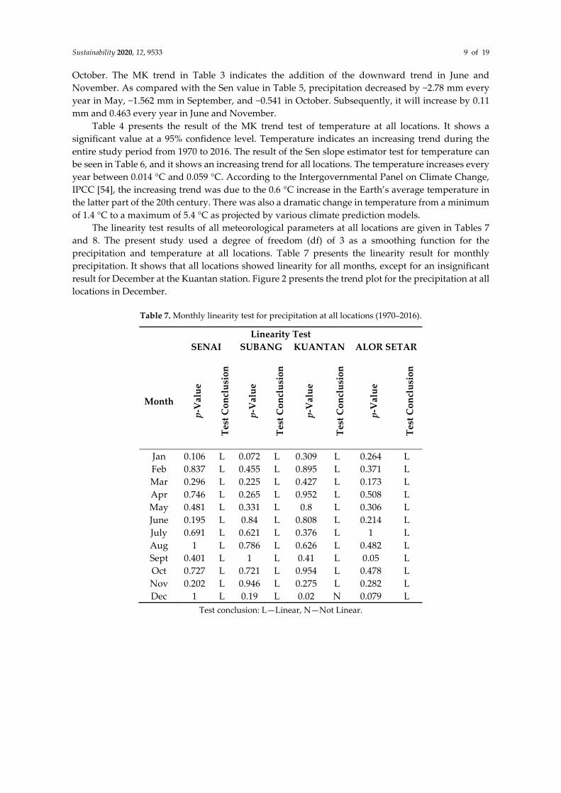
The linearity test results of all meteorological parameters at all locations are given in Tables 7

and 8. The present study used a degree of freedom (df) of 3 as a smoothing function for the

precipitation and temperature at all locations. Table 7 presents the linearity result for monthly

precipitation. It shows that all locations showed linearity for all months, except for an insignificant

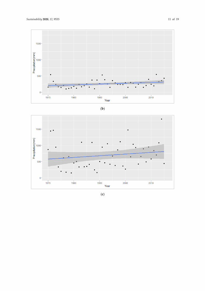
result for December at the Kuantan station. Figure 2 presents the trend plot for the precipitation at all

locations in December.

Table 7. Monthly linearity test for precipitation at all locations (1970–2016).

Linearity Test


Month

p-V

alu

e

Tes

t C

on

clu

sio

n

p-V

alu

e

Tes

t C

on

clu

sio

n

p-V

alu

e

Tes

t C

on

clu

sio

n

p-V

alu

e

Tes

t C

on

clu

sio

n

Jan 0.106 L 0.072 L 0.309 L 0.264 L

Feb 0.837 L 0.455 L 0.895 L 0.371 L

Mar 0.296 L 0.225 L 0.427 L 0.173 L

Apr 0.746 L 0.265 L 0.952 L 0.508 L

May 0.481 L 0.331 L 0.8 L 0.306 L

June 0.195 L 0.84 L 0.808 L 0.214 L

July 0.691 L 0.621 L 0.376 L 1 L

Aug 1 L 0.786 L 0.626 L 0.482 L

Sept 0.401 L 1 L 0.41 L 0.05 L

Oct 0.727 L 0.721 L 0.954 L 0.478 L

Nov 0.202 L 0.946 L 0.275 L 0.282 L

Dec 1 L 0.19 L 0.02 N 0.079 L

Test conclusion: L—Linear, N—Not Linear.


Table 8. Monthly linearity test for temperature at all locations (1970–2016).

Linearity Test


Month

p-v

alu

e

Tes

t C

on

clu

sio

n

p-v

alu

e

Tes

t C

on

clu

sio

n

p-v

alu

e

Tes

t C

on

clu

sio

n

p-v

alu

e

Tes

t C

on

clu

sio

n

Jan 0.096 L 0.216 L 0.66 L 0.082 L

Feb 0.079 L 0.6 L 0.474 L 0.648 L

Mar 0.501 L 0.451 L 0.823 L 0.559 L

Apr 0.113 L 0.607 L 0.788 L 0.68 L

May 0.349 L 0.158 L 0.315 L 0.765 L

June 0.0 N 0.598 L 0.49 L 0.497 L

July 0.014 N 0.481 L 0.464 L 0.14 L

Aug 0.297 L 0.62 L 0.296 L 0.135 L

Sept 0.048 N 0.268 L 0.399 L 0.101 L

Oct 0.115 L 0.549 L 0.913 L 0.18 L

Nov 0.068 L 0.139 L 0.477 L 1 L

Dec 0.368 L 0.031 N 0.431 L 1 L

Test conclusion: L—Linear, N—Not Linear.

(a)


(b)

(c)


(d)

Figure 2. Plot for precipitation in December for Senai (a), Subang (b), Kuantan (c), and Alor Setar (d).

Figure 2 indicates that there is a pattern in the precipitation at Kuantan in comparison with

other locations. The p-values for Senai, Subang, and Alor Setar are significant at 1, 0.19, and 0.079,

respectively, while Kuantan has a p-value of 0.02. Kuantan indicates a large amount of rainfall with

more than 1500 mm rainfall for a particular month as compared with other locations. The

precipitation patterns in Senai, Subang, and Alor Setar are almost alike. The divergence of the

monthly distribution precipitation pattern in Kuantan is presented by a scattered plot for the month.

Table 8 presents the result of the linearity test for temperature. Kuantan and Alor Setar

exhibited linearity in temperature for all months. Subang indicated the same pattern except for the

amount of precipitation in December. Senai indicated a nonlinear temperature pattern for the

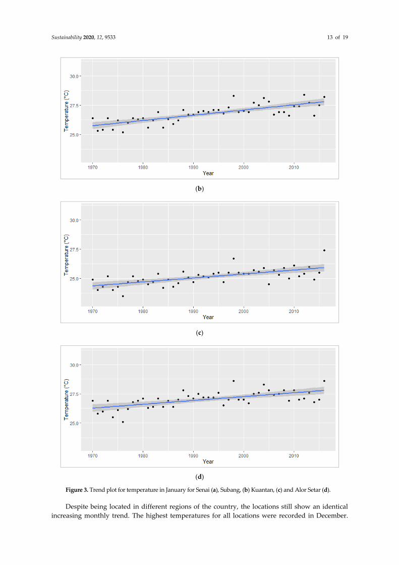
months of June, July, and September. Figure 3 presents the trend plot for temperature at all locations

in January. The p-values for Senai, Subang, Kuantan, and Alor Setar are 0.096, 0.216, 0.66, and 0.082,

respectively. The plot shows that the temperatures at all locations have a linear pattern and the

pattern has increased every year since 1970.

(a)


(b)

(c)

(d)

Figure 3. Trend plot for temperature in January for Senai (a), Subang, (b) Kuantan, (c) and Alor Setar (d).

Despite being located in different regions of the country, the locations still show an identical

increasing monthly trend. The highest temperatures for all locations were recorded in December.


Figure 2 shows that Kuantan received the highest amount of rainfall in December. However, the

highest temperature was still recorded for January.

5. Discussion

The MK trend test gives an interesting insight into monthly temperature and monthly

precipitation trends for the selected locations. From the precipitation of the MK test result, it

indicates that most of the months showed no trend for all locations. Table 3 displays trend results for

monthly precipitation. Senai indicates an increasing trend with a Z value 0.254 in August, while, for

other months, no trend was depicted. Subang indicates an increasing trend only in January, August,

November, and December with Z values 0.236, 0.246, 0.333, and 0.247, respectively. Kuantan

depicted an increasing trend only in August, the same as Senai with a Z value 0.254 and no trend

shown for other months. Alor Setar indicates a decreasing trend in May, June, September, October,

and November with Z values of −0.325, −0.255, −0.407, −0.286 and −0.21. However, other months did

not show any trend. Table 4 displays the trend result of monthly temperature and shows an upward

trend in all months for all locations.

Table 5 presents the result of the Sen slope for monthly precipitation. Senai indicates an upward

trend in January, March, April, and August to December. Subang indicates an upward trend in all

months. Kuantan indicates an upward trend in January, March, May, August, and December. Alor

Setar depicted a downward trend in May, September and October. Table 7 presents a linearity test

for monthly precipitation and all months exhibit linearity for all locations. Despite the fact that the

number of months with no trend is more than the number of months with a trend, Malaysia climate

change phenomena should not be ignored. It is important to consider the previous flood history in

Malaysia such as in Senai and Kuantan as a result of the heavy rainfall events in December 2014 and

December 2006. Increased rainfall causes serious flooding in Malaysia almost every year due to

climate change [55].

Although floods are natural phenomena, uncontrolled development, indiscriminate land

clearing, and other human activities increase the severity of floods [56]. Climate change is currently

debated as an anthropological phenomenon related to environmental systems [57]. Kuantan

experienced flooding in the past due to anthropogenic influence causing alterations in temperature

and torrential rain [58].

Table 4 and Table 6 present the results of the MK trend test and the Sen slope test for monthly

temperature. Both results show an increasing trend in all months for all locations. All locations

showed a clear increasing temperature trend for all months. This is quite worrying as many studies

have shown that the Earth is experiencing serious global warming. Brown [59] contended that the

change in temperatures indicates a significant positive trend throughout the globe since 1950. Wong

et al. [60] shows that the annual mean temperature trend has significantly increased at the 95%

confidence level at about 0.32 °C per decade in Peninsular Malaysia. Senai, Subang, Kuantan, and

Alor Setar are rapidly developing, causing the increasing temperature. Increasing temperature will

have an immediate impact on rainfall distribution, where it will lead to flooding.

The result of the present study shows a similar outcome to other researchers. Mayowa [61]

showed there was a substantial increase in annual rainfall during the monsoon season, especially on

the east coast of Peninsular Malaysia. Kuantan indicates an increasing trend during this monsoon,

while Huang [6] discovered that an increasing rainfall trend occurred for most months at a few

stations in the west region of Peninsular Malaysia, and the Sen slope indicates an upward trend in all

months for Subang. During the Northeast Monsoon, the northern region of Peninsular Malaysia

experiences drought due to less precipitation [62]. Alor Setar confirms this, indicating a downward

trend and no trend for most of the month as a result of the monsoon [63]. Wong [60] reported that

the rainfall trend during Northeast Monsoon significantly increased at the 95% confidence level in

all regions of Peninsular Malaysia, and Senai indicated a similar outcome during this monsoon.

Apart from that, temperature trends show a significant increasing trend, especially in the western

region of Peninsular Malaysia [64]. This corresponds to the results of the present study. Hashim [65]

showed that there is an increasing trend for temperature from 1970 to 2005 in the urban areas of


Kuantan and the western regions of Peninsular Malaysia. The Director of the Malaysian

Meteorological Department confirmed in the local newspaper Sinar Harian [66] that the increase in

temperature might be due to the Southwest Monsoon, which usually brings hot and dry weather

conditions.

Understanding meteorological trends is important for planning and management, especially

with respect to sustainability issues such as water resources, construction projects, and agriculture.

An increase in temperature year on year will lead to multiple adverse effects on the earth and put it

at risk. Adnan found that increases in flooding are likely due to changes in precipitation resulting

from land use changes. According to Rahman [67], raising awareness is key to ensuring the

sustainability of land use and sustaining the environment.

As reported by the IPCC [68], climate change leads to many adverse impacts. Flooding will

harm agriculture. Additionally, it will impair economic growth. At the same time, increasing

temperature will cause sea-level rise, melting snow, and glaciers. In addition to understanding the

meteorological parameters, some actions can be taken to reduce the increasing number of

precipitation events and temperature increases each year to sustain the normal environment.

According to Denchak [69], healing our earth can be started in our own home. Everyone can

contribute to sustaining the environment. Malaysia as a developed country can make a good effort to

achieve sustainable development. Cooperation among the government, private sector, and

Malaysian citizens will have a positive impact on the environment and climate planning [70].

6. Conclusions

As the pattern of precipitation and temperature varies from one region to another due to the

strong influence of the monsoons, an investigation of monthly trend meteorological parameters was

conducted. Four locations in Peninsular Malaysia, representing the northern, southern, eastern, and

western regions of Malaysia over a period of 47 years, were selected. Thus, a whole vision of a

monthly monotonic trend was developed for these two main meteorological parameters. Statistical

analysis was conducted as an initial step to understand the data. The MK trend test, the Sen slope

estimator, and linearity test are techniques widely used for environmental and climate studies. The

MK trend test for precipitation did not exhibit any trend except for the month of August at Senai,

Subang, and Kuantan, whereas temperature shows an increasing monthly trend during the entire

study period of 47 years. The Sen slope results also demonstrate an increasing trend for all locations.

The linearity test for precipitation indicates linearity for all months, except for the month of

December in Kuantan. For temperature, only Kuantan and Alor Setar showed linearity for all

months. All the methods provide a result explaining the trend for all the meteorological parameters.

The MK trend test and the Sen slope estimator give a clear view of the precipitation and temperature

trend in some of the regions of Peninsular Malaysia. The Sen value indicates how precipitation and

temperature increase and decrease every year.

The substantial economic activities in most of the study areas may have environmental

implications. In conclusion, the findings from this study may give useful information regarding the

monthly trend of meteorological parameters in Senai, Subang, Kuantan, and Alor Setar. In addition,

they can contribute to governmental and institutional planning. Therefore, investigating trends in

meteorological parameters gives an insight into climate conditions, especially in Peninsular Malaysia.

Author Contributions: In this article, five (5) authors contributed their ideas and works throughout the process

to complete the article. The first author (F.M.S.) is the main provider for this article. She contributed the idea of

the article, followed by writing the original draft, formal analysis and submitting the article. The second author

(F.M.H.) acted as corresponding author and was responsible for supervision, proposing suitable methods and

software to be used in the article, and he received a grant that provided funding for the research. The third

author (M.E.T.) acted as a second corresponding author responsible for suggesting additions to the original

draft, visualization structure, investigation, proposing suitable software and helping in reviewing and editing,

and he received a grant that also provided funding for the research. The fourth author (O.J.) provided the

resources of raw data and provided the main idea in the conceptualization of the project. The fifth author (H.T.)


was responsible for the review, editing and checking of the whole article. All authors have read and agreed to

the published version of the manuscript.

Funding: This research was funded by the National University of Malaysia via research grant number

(GUP-2020-013) and (KRA-2017-035).

Acknowledgments: The authors would like to acknowledge the Earth Observation Centre, National University

of Malaysia for providing the data for this research.

Conflicts of Interest: The authors declare no conflict of interest.

References

1. Olcese, L.E.; Toselli, B.M. Meteorology, and Atmospheric Physics Effects of Meteorology and Land use on

Ambient Measurements of Primary Pollutants in C6rdoba City Argentina. Meteorol. Atmos. Phys. 1997, 248,

241–242.

2. Qian, W.; Lin, X. Regional trends in recent precipitation indices in China. Meteorol. Atmos. Phys. 2005, 207,

193–194, doi:10.1007/s00703-004-0101-z.

3. Funatsu, B.M.; Dubreuil, V.; Racapé, A. Perceptions of climate and climate change by Amazonian

communities. Glob. Environ. Chang. 2019, 57, doi:10.1016/j.gloenvcha.2019.05.007.

4. Malaysian Meteorological Department. Available online: http://www.met.gov.my/ (accessed on 6 May

2014).

5. Chew, T. The Monsoon Seasons in Malaysia. Available online:

http://www.expatgo.com/my/2013/06/28/the-monsoon-seasons-in-malaysia/ (accessed on 18 May 2017).

6. Huang, Y.F.; Puah, Y.J.; Chua, K.C.; Lee, T.S. Analysis of monthly and seasonal rainfall trends using the

Holt’s test. Int. J. Climatol. 2014, doi:10.1002/joc.4071.

7. Fonseca, D.; Carvalho, M.J.; Rocha, A. Recent trends of extreme temperature indices for the Iberian

Peninsula. Phys. Chem. Earth 2016, 94, 66–76, doi:10.1016/j.pce.2015.12.005.

8. Miguel, M.; Nilsson, E.; Uamusse, M.M. Climate Change observations into Hydropower in Mozambique.

Energy Procedia 2017, 138, 592–597, doi:10.1016/j.egypro.2017.10.165.

9. Hansen, J.; Sato, M.; Ruedy, R.; Lo, K.; Lea, D.W.; Medina-elizade, M. Global Temperature Change. Proc.

Natl. Acad. Sci. USA 2006, doi:10.1073/pnas.0606291103.

10. Li, Y.; Li, G.; Zeng, Q.; Liang, F.; Pan, X. Projecting temperature-related years of life lost under different

climate change scenarios in one temperate megacity, China. Environ. Pollut. 2018, 233, 1068–1075,

doi:10.1016/j.envpol.2017.10.008.

11. Tzanis, C.G.; Koutsogiannis, I.; Philippopoulos, K.; Deligiorgi, D. Recent climate trends over Greece.

Atmos. Res. 2019, 230, doi:10.1016/j.atmosres.2019.104623.

12. Shaaban, A.J. Impact of Climate Change on Malaysia; NAHRIM: Bangi, Malaysia, 2013.

13. Nam, W.H.; Baigorria, G.A. How climate change has affected the spatio- temporal patterns of

precipitation and temperature at various time scales in North Korea. Int. J. Climatol. 2015, 493,

doi:10.1002/joc.4378.

14. Akhtar, M.P. Non Parametric Trend Analysis of Climate Change in Lower Bagmati River Basin in

Northern India. Int. J. Sci. Eng. Technol. 2015, 4, 461–465.

15. Rosmann, T.; Domínguez, E.; Chavarro, J. Journal of Hydrology: Regional Studies Comparing trends in

hydrometeorological average and extreme data sets around the world at different time scales. Biochem.

Pharmacol. 2016, 5, 200–212, doi:10.1016/j.ejrh.2015.12.061.

16. Sang, Y.; Wang, Z.; Liu, C. Comparison of the MK test and EMD method for trend identification in

hydrological time series. J. Hydrol. 2014, 510, 293–298, doi:10.1016/j.jhydrol.2013.12.039.

17. Ho, K.; Tang, D. Science of the Total Environment Climate change in Malaysia: Trends, contributors,

impacts, mitigation and adaptations. Sci. Total Environ. 2019, 650, 1858–1871,

doi:10.1016/j.scitotenv.2018.09.316.

18. World Meteorologizal Organizational. Climate Data Homogenization. Available online:

https://www.wmo.int/pages/prog/wcp/wcdmp/CA_4.php (accessed on 30 August 2020).

19. Damen, M. Data Homogenization. Available online: http://www.charim.net/datamanagement/63#

(accessed on 1 September 2020).


20. Cristina, A.; Amílcar, C. Homogenization of Climate Data: Review and New Perspectives Using

Geostatistics. Math. Geosci. 2009, 41, doi:10.1007/s11004-008-9203-3.

21. Iskandar Malaysia. Available online: http://iskandarmalaysia.com.my/ (accessed on 25 May 2020).

22. Wolanski, E. The Environment in Asia Pacific Harbours; Springer Science & Business Media: Townsville,

Australia, 2006; p. 349.

23. Annisa, U. Faktor- faktor yang Mempengaruhi Cuaca dan Iklim di Malaysia. Available online:

https://www.slideshare.net/annisaulhusna18/faktor-yang-mempengaruhi-cuaca-iklim-malaysia/

(accessed on 20 July 2020).

24. Weather and Climate. Climate in Subang Jaya. Available online:

https://weather-and-climate.com/average-monthly-Rainfall-Temperature-Sunshine,subang-jaya-selangor-

my,Malaysia (accessed on 18 May 2020).

25. Pohlert, T. Package Trend 2020, 1–37. Available online:

https://cran.r-project.org/web/packages/trend/trend.pdf (accessed on 20 July 2020).

26. Bowman, A.; Azzalini, A. Package ‘sm’ 2019, 1–74. Available online:

https://cran.r-project.org/web/packages/sm/sm.pdf (accessed on 17 September 2020).

27. Mavromatis, T.; Stathis, D. Response of the water balance in Greece to temperature and precipitation

trends. Theor. Appl. Climatol. 2010, 104, 13–24, doi:10.1007/s00704-010-0320-9.

28. Hefzul, S.; Ur, M.T.; Azizul, M.; Hussain, M. Analysis of seasonal and annual rainfall trends in the

northern region of Bangladesh. Atmos. Res. 2016, 176–177, 148–158, doi:10.1016/j.atmosres.2016.02.008.

29. Yue, S.; Wang, C. The Mann-Kendall Test Modified by Effective Sample Size to Detect Trend in Serially

Correlated Hydrological Series. Water Resour. Manag. 2004, 18, 201–218,

doi:10.1023/B:WARM.0000043140.61082.60.

30. Goenster, S.; Wiehle, M.; Gebauer, J.; Mohamed, A.; Stern, R.D.; Buerkert, A. Daily rainfall data to identify

trends in rainfall amount and rainfall-induced agricultural events in the Nuba Mountains of Sudan. J.

Arid. Environ. 2015, 122, 16–26, doi:10.1016/j.jaridenv.2015.06.003.

31. Altin, T.B.; Barak, B. Changes and trend in total yearly precipitation of the Antalya district, Turkey.

Procedia Soc. Behav. Sci. 2014, 120, 586–599, doi:10.1016/j.sbspro.2014.02.139.

32. Araghi, A.; Adamowski, J.; Rajabi, M. Detection of trends in days with thunderstorms in Iran over the

past five decades. Atmos. Res. 2016, 172–173, 174–185, doi:10.1016/j.atmosres.2015.12.022.

33. Mann, H.B. Nonparametric Tests Against Trend. Econometrica 1945, 13, 245–259.

34. Kendall, M. Rank Correlation Methods; Griffin: London, UK, 1975.

35. Mozejko, J. Detecting and Estimating Trends of Water Quality Parameters. In Water Quality Monitoring

and Assessment; InTech: Rijeka, Croatia, 2012; pp. 95–120.

36. Tabari, H.; Marofi, S.; Aeini, A.; Talaee, P.H.; Mohammadi, K. Trend analysis of reference

evapotranspiration in the western half of Iran. Agric. For. Meteorol. 2011, 151, 128–136,

doi:10.1016/j.agrformet.2010.09.009.

37. Sen, P.K. Estimates of the Regression Coefficient Based on Kendall’ s Tau. J. Am. Stat. Assoc. 1968, 63,

1379–1389.

38. Bowman, A.W.; Azzalini, A. Applied Smoothing Techniques for Data Anlysis; Oxford University Press:

Oxford, UK, 1997.

39. Brownlee, J. Linear Regression for Machine Learning. Available online:

https://machinelearningmastery.com/linear-regression-for-machine-learning/ (accessed on 1 September

2020).

40. Motiee, H.; McBean, E. An assessment of long-term trends in hydrologic components and implications for

water levels in Lake Superior. Hydrol. Res. 2009, 40, 564, doi:10.2166/nh.2009.061.

41. Cleveland, W.S. Robust Locally Weighted Regression and Smoothing Scatterplots. J. Am. Stat. Assoc. 1979,

74, 829–836.

42. Dhir, R. Data Smoothing Definition. Investopedia. Available online:

https://www.investopedia.com/terms/d/data-smoothing.asp (accessed on 30 August 2020).

43. Fan, J.; Gijbels, I. Variable Bandwidth and Local Linear Regression Smoothers. Ann. Stat. 1992, 20, 2008–

2036.


44. Chandler, R.; Scott, M. Statistical Methods for Trend Detection and Analysis in the Environmental Sciences;

John Wiley & Sons, Ltd.: West Sussex, UK, 2011. doi:10.1002/9781119991571.

45. Kothyari, U.; Singh, V.P. Rainfall and Temperature Trends in India. Hydrol. Process. 1996, 10, 357–372,

doi:10.1002/(SICI)1099-1085(199603)10:3<357::AID-HYP305>3.0.CO;2-Y.

46. Keele, L. Semiparametric Regression for the Social Sciences; John Wiley & Sons, Ltd.: Hoboken, NJ, USA,

2008.

47. Stone, M. Cross-Validatory Choice and Assessment of Statistical Predictions. J. R. Stat. Soc. 1974, 36, 111–

147, doi:10.2307/2984809.

48. Craven, P.; Wahba, G. Numerische Mathematik. Numer. Math. 1979, 31, 377–403.

49. Akaike, H. Information Theory and an Extension of the Maximum Likelihood Principle. In 2nd

International Symposium on Information Theory; Springer: New York, NY, USA, 1973; pp. 610–624.

50. Hurvich, C.M.; Simonoff, J.S.; Tsai, C.L. Smoothing Parameter Selection in Nonparametric Regression

Using an Improved Akaike Information Criterion. J. R. Stat. Soc. 1998, 60, 271–293.

51. Silverman, B.W. A Fast and Efficient Method for Smoothing Parameter Choice in Spline Regression. J. Am.

Stat. Assoc. 2014, 79, 584–589.

52. Craven, P.; Wahba, G. Smoothing Noisy Data with Spline Functions. Numer. Math. 1979, 403, 377–403.

53. Mohamad Hamzah, F. Statistical Analysis of Freshwater Parameters Monitored at Different Temporal

Resolutions. Ph.D. Thesis, University of Glasgow, Glasgow, Scotland, 2012.

54. IPCC. IPCC, 2013: Summary for Policymakers. In Climate Change 2013: The Physical Science Basis.

Contribution of Working Group I to the Fifth Assessment Report of the Intergovernmental Panel on Climate

Change; Cambridge University Press: Cambridge, UK; New York, NY, USA, 2013.

55. Mohammed, N.; Edwards, R.; Gale, A.; Mohammed, N. ScienceDirect ScienceDirect ScienceDirect

Optimisation of Flooding Recovery for Malaysian Universities Optimisation of Flooding Recovery for

Malaysian Universities. Procedia Eng. 2018, 212, 356–362.

56. Chan, N.W. Sustainable management of rivers in Malaysia : Involving all stakeholders Sustainable

Management of Rivers in Malaysia: Involving All Stakeholders. Int. J. River Manag. 2005,

doi:10.1080/15715124.2005.9635254.

57. Loo, Y.Y.; Billa, L.; Singh, A. Effect of climate change on seasonal monsoon in Asia and its impact on the

variability of monsoon rainfall in Southeast Asia. Geosci. Front. 2014, 1–7, doi:10.1016/j.gsf.2014.02.009.

58. Zaidi, S.M.; Akbari, A.; Ishak, W.M.F. A Critical review of Floods History in Kuantan River Basin:

Challenges and Potential Solutions. Int. J. Civ. Eng. Geo-Environ. 2014, 5, 3–5.

59. Brown, S.J.; Caesar, J.; Ferro, C.A.T. Global changes in extreme daily temperature since 1950. J. Geophys.

Res. 2008, 113, doi:10.1029/2006JD008091.

60. Wong, C.; Yusop, Z.; Ismail, T. Trend of Daily Rainfall and Temperature In Peninsular Malaysia Based on

Gridded Data Set. Int. J. Geomate 2018, 14, 65–72.

61. Mayowa, O.O.; Pour, S.H.; Shahid, S. Trends in rainfall and rainfall-related extremes in the east coast of

peninsular Malaysia. J. Earth Syst. Sci. 2015, 124, 1609–1622.

62. Jamaludin, S.; Mohd Deni, W.Z.; Zin, W.; Jemain, A.A. Trends in Peninsular Malaysia Rainfall Data

During the Southwest Monsoon and Northeast Monsoon Seasons. Sains Malays. 2010, 39, 1975–2004.

63. Chooi, T.K. Trends of rainfall regime in Peninsular Malaysia during northeast and southwest monsoons. J.

Phys. Conf. Ser. 2018, 995, 2–5.

64. Valley, K.; Shahrul, M.; Nadzir, M.; Juneng, L. Observed Trends in Extreme Temperature over the. Adv.

Atmos. Sci. 2019, 36, 1355–1370.

65. Hashim, N.M. The impact of global warming trends on urban livability in Malaysia: An analysis. Malays.

J. Soc. Space 2010, 2, 72–88.

66. Sinar, H. Malaysia Dilandacuaca Panas. Available online:

http://www.sinarharian.com.my/malaysia-dilanda-cuaca-panas-1.17279 (accessed on 13 July 2015).

67. Rahman, H.A. Brief Review An Overview of Environmental Disaster in Malaysia and Preparedness

Strategies. Iran. J. Public Health 2015, 43, 17–24.

68. IPCC. Impacts of Climate Change. Available online:

https://www.activesustainability.com/climate-change/impacts-climate-change/ (accessed on 25 June

2020).


69. Denchak, M. How You Can Stop Global Warming. Available online:

https://www.nrdc.org/stories/how-you-can-stop-global-warming (accessed on 13 April 2020).

70. Mokthsim, N.; Salleh, K.O. Malaysia’s Efforts Towards Achieving a Sustainable Developmnet: Issues,

Challenges and Prospects. Procedia Soc. Behav. Sci. 2014, 120, 299–307, doi:10.1016/j.sbspro.2014.02.107.

Publisher’s Note: MDPI stays neutral with regard to jurisdictional claims in published maps and institutional

affiliations.

© 2020 by the authors. Licensee MDPI, Basel, Switzerland. This article is an open access

article distributed under the terms and conditions of the Creative Commons Attribution

(CC BY) license (http://creativecommons.org/licenses/by/4.0/).

trend and linearity analysis of meteorological parameters in

Documents