LED PWM Dimming Linearity Investigation L. Svilainis Signal Processing Department, Kaunas University o f Technology, Studentu str. 50, LT-51368 Kaunas, Lithuania, phone +370 37 300532; fax. +370-37-352998; e-mail: svilnis@ktu.lt Abstract LED PWM dimming application for large scale LED video displays is analyzed. The

need for short light pulse duration is outlined. PWM dimming with short driving pulses is investigated experimentally. The LED response time skew introduces the nonlinearity for PWM dimming. For LED response time skew estimation, a method is suggested that has been successfully applied to measure some of today�s market representative LEDs. PWM dimming nonlinearity can be forecasted using the estimated skew. For a particular driving configuration, it is indicated that LED PWM dimming fails to satisfy the required 14 bit output coding together with the image refresh frequency of 400 Hz. A rough investigation demonstrates that the skew is quite stable. Therefore, the nonlinearity correction for the PWM pulse durations shorter than the skew value should be possible.

Keywords LED dimming, PWM linearity, LED response time 1. Introduction Light Emitting Diode (LED) is about to hit its 50 years anniversary. Due to increasing

efficiency of LEDs compared to incandescent and even luminescent lamps, more and more often they are accepted as a light source for many applications. This technology also presents an option for information display on a flat screen offering a wide viewing angle and a bright, clear image suitable for outdoor application [1]. On large scale LED video displays, LED application imposes certain requirements for screen pixel gray scale creation.

The ease of dimming by PWM makes it attractive for large scale LED video screens. This type of control can be readily implemented in a digital form. Thanks to inexpensive and stable frequency sources, a steady driving over a wide range of intensities can be ensured. But is the LED response stable?

The aim of this paper is to analyze the LED PWM dimming application on LED video displays outlining the need for short driving pulse durations and investigating the dimming linearity and stability.

2. Need for a Short Driving Pulse LED luminance can be controlled by the diode forward current [2]. Modern LED video

screens are demanded to be in color. But the forward current affects the LED emission wavelength. If LED could be operated at a constant current, this would ensure the screen color gamut stability. The most convenient method for LED dimming without altering the current is the pulse-width-modulation (PWM) [3]. Average power, thereby the expected light output, of PWM should be linearly proportional to pulse duration:

TYY on

n

, (1)

id205822187 pdfMachine by Broadgun Software - a great PDF writer! - a great PDF creator! - http://www.pdfmachine.com http://www.broadgun.com

here T is PWM period, Yn is the maximum luminance (100% duty), on is PWM pulse duration when LED is on and Y is the resulting luminance. PWM period usually is divided into 2N levels (discrete time intervals). Then N bits are required to code the pixel intensity with PWM. Then time step interval min is the following:

N

T

2min , (2)

The smallest reachable time interval min defines the lowest PWM dimming intensity attained. The nonlinearity of the human sense of light [4] requires specific approach to light

coding. The image camera capturing mimics the human visual system. This nonlinearly coded (gamma-corrected) signal is transformed back to linear intensity at the display (inverse gamma), using a nonlinear voltage-to-intensity response inherent for the CRT. Coding the video image intensity into a gamma-corrected signal makes the maximum perceptual use of the channel. When an image has to be displayed on the linear response display (the LED video screen driven with PWM), an inverse gamma correction is a must. The imaging system requires an inverse gamma correction to mimic the nonlinear CRT display response. This means that the higher number of LED brightness levels is needed for output since some of the codes shall be thrown away for the sake of linearization in human perception. Mathematically, the conventional 24 bit coded pixel color 8 bit input code Cin conversion to the gamma-corrected (CRT mimicking) code CGamma with resolution of N bits can be expressed as follows:

12

255Nin

GammaC

roundC

. (3)

Such gamma correction will exhibit some rounding approximation error:

%1001

12255

%100

12255

12255

Nin

Gamma

Nin

NinGamma

approxC

C

C

CC

. (4)

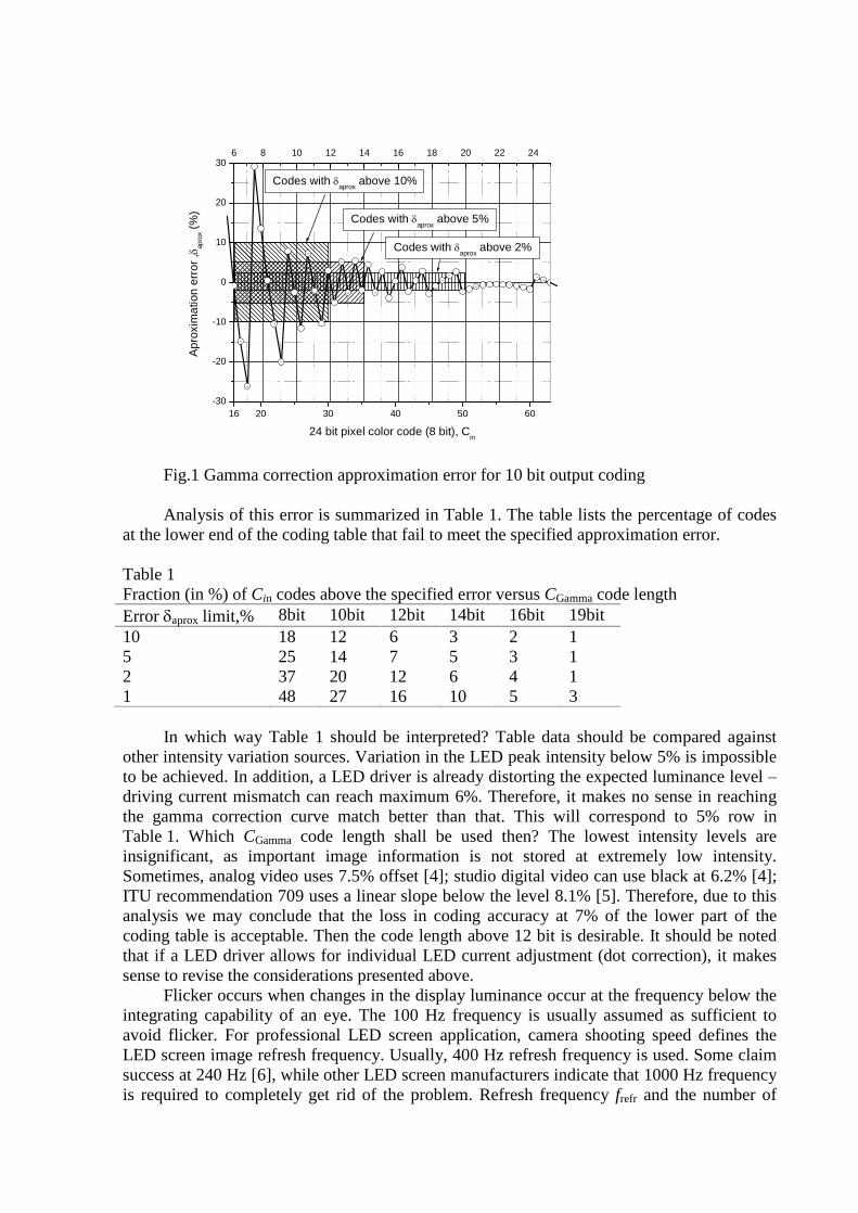
For example, when applying a 2.4 gamma correction only a code using 19 bit resolution is capable of monotonic variance � every change in an input code (8 bits) causes change in an output code within the same direction. An approximation error will be large at the lower end of the coding table � this is clearly demonstrated by an error graph for 10 bit output coding presented in Fig. 1.

16 20 30 40 50 60-30

-20

-10

0

10

20

306 8 10 12 14 16 18 20 22 24

Codes with aprox

above 2%

Codes with aprox

above 5%

Codes with aprox

above 10%A

prox

imat

ion

erro

r ,

apro

x (%

)

24 bit pixel color code (8 bit), Cin

Fig.1 Gamma correction approximation error for 10 bit output coding Analysis of this error is summarized in Table 1. The table lists the percentage of codes

at the lower end of the coding table that fail to meet the specified approximation error.

Table 1 Fraction (in %) of Cin codes above the specified error versus CGamma code length Error aprox limit,% 8bit 10bit 12bit 14bit 16bit 19bit 10 18 12 6 3 2 1 5 25 14 7 5 3 1 2 37 20 12 6 4 1 1 48 27 16 10 5 3

In which way Table 1 should be interpreted? Table data should be compared against

other intensity variation sources. Variation in the LED peak intensity below 5% is impossible to be achieved. In addition, a LED driver is already distorting the expected luminance level � driving current mismatch can reach maximum 6%. Therefore, it makes no sense in reaching the gamma correction curve match better than that. This will correspond to 5% row in Table 1. Which CGamma code length shall be used then? The lowest intensity levels are insignificant, as important image information is not stored at extremely low intensity. Sometimes, analog video uses 7.5% offset [4]; studio digital video can use black at 6.2% [4]; ITU recommendation 709 uses a linear slope below the level 8.1% [5]. Therefore, due to this analysis we may conclude that the loss in coding accuracy at 7% of the lower part of the coding table is acceptable. Then the code length above 12 bit is desirable. It should be noted that if a LED driver allows for individual LED current adjustment (dot correction), it makes sense to revise the considerations presented above.

Flicker occurs when changes in the display luminance occur at the frequency below the integrating capability of an eye. The 100 Hz frequency is usually assumed as sufficient to avoid flicker. For professional LED screen application, camera shooting speed defines the LED screen image refresh frequency. Usually, 400 Hz refresh frequency is used. Some claim success at 240 Hz [6], while other LED screen manufacturers indicate that 1000 Hz frequency is required to completely get rid of the problem. Refresh frequency frefr and the number of

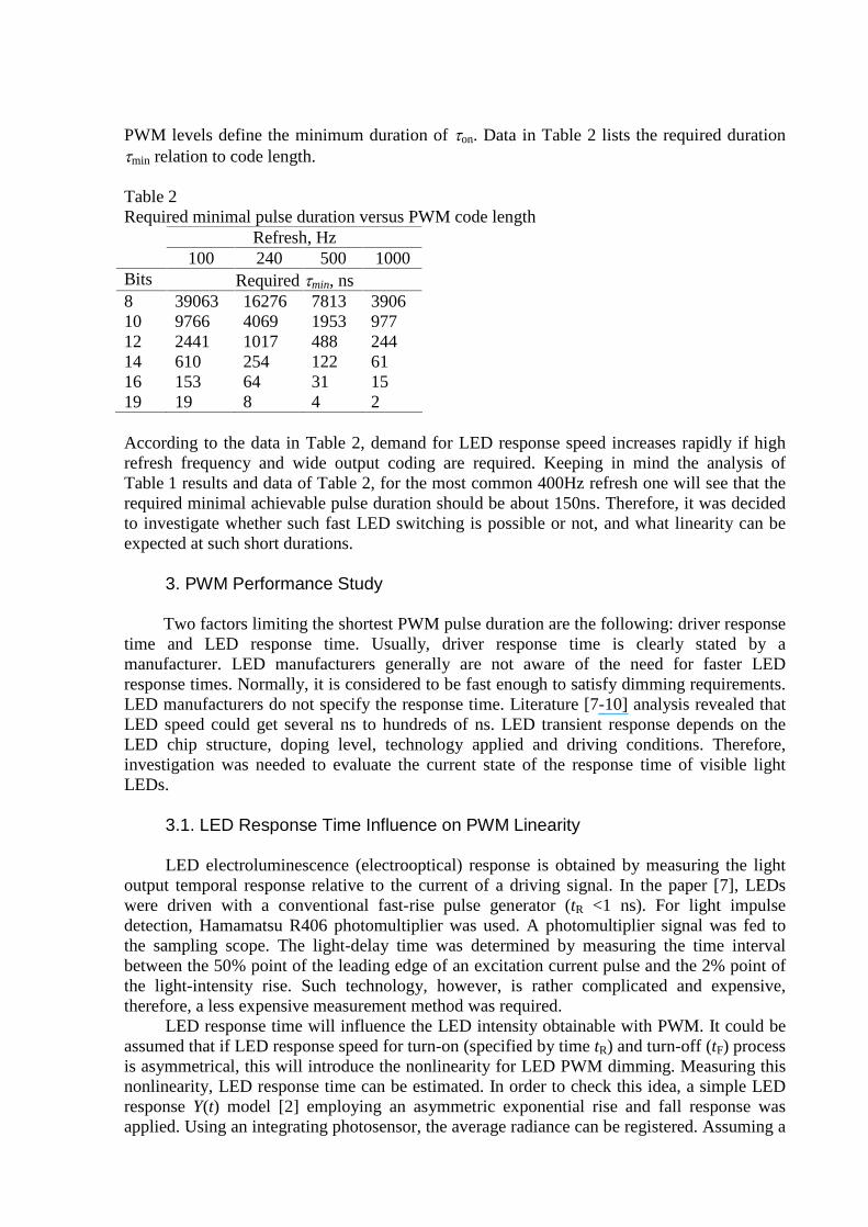
PWM levels define the minimum duration of on. Data in Table 2 lists the required duration min relation to code length.

Table 2 Required minimal pulse duration versus PWM code length Refresh, Hz 100 240 500 1000 Bits Required min, ns 8 39063 16276 7813 3906 10 9766 4069 1953 977 12 2441 1017 488 244 14 610 254 122 61 16 153 64 31 15 19 19 8 4 2

According to the data in Table 2, demand for LED response speed increases rapidly if high refresh frequency and wide output coding are required. Keeping in mind the analysis of Table 1 results and data of Table 2, for the most common 400Hz refresh one will see that the required minimal achievable pulse duration should be about 150ns. Therefore, it was decided to investigate whether such fast LED switching is possible or not, and what linearity can be expected at such short durations.

3. PWM Performance Study Two factors limiting the shortest PWM pulse duration are the following: driver response

time and LED response time. Usually, driver response time is clearly stated by a manufacturer. LED manufacturers generally are not aware of the need for faster LED response times. Normally, it is considered to be fast enough to satisfy dimming requirements. LED manufacturers do not specify the response time. Literature [7-10] analysis revealed that LED speed could get several ns to hundreds of ns. LED transient response depends on the LED chip structure, doping level, technology applied and driving conditions. Therefore, investigation was needed to evaluate the current state of the response time of visible light LEDs.

3.1. LED Response Time Influence on PWM Linearity LED electroluminescence (electrooptical) response is obtained by measuring the light

output temporal response relative to the current of a driving signal. In the paper [7], LEDs were driven with a conventional fast-rise pulse generator (tR <1 ns). For light impulse detection, Hamamatsu R406 photomultiplier was used. A photomultiplier signal was fed to the sampling scope. The light-delay time was determined by measuring the time interval between the 50% point of the leading edge of an excitation current pulse and the 2% point of the light-intensity rise. Such technology, however, is rather complicated and expensive, therefore, a less expensive measurement method was required.

LED response time will influence the LED intensity obtainable with PWM. It could be assumed that if LED response speed for turn-on (specified by time tR) and turn-off (tF) process is asymmetrical, this will introduce the nonlinearity for LED PWM dimming. Measuring this nonlinearity, LED response time can be estimated. In order to check this idea, a simple LED response Y(t) model [2] employing an asymmetric exponential rise and fall response was applied. Using an integrating photosensor, the average radiance can be registered. Assuming a

monochromatic LED emission, this can be assigned to an average luminance. Fig. 2 may be referred to for the most informative modeling results. Pulse repetition period T was 400 ns. Various tR and tF time combinations were evaluated. The light pulse energy is calculated by integrating the electrooptical response Y(t) over the PWM period. The ideal light pulse energy is assumed to be equal to the full-scale light output value Yn multiplied by duty on/T. The nonlinearity error is a difference of the two, normalized by full-scale light output value Yn and expressed in percents:

%100

1

0

n

onn

T

onskewed Y

TYdttY

T

. (5)

This is the expression of average luminance supposed to be sensed by a human eye or averaging photosensor (radiance).

0 20 40 60 80 100-10

-8

-6

-4

-2

0

2

tR=82ns, t

F=2ns

tR=120ns, t

F=40ns

tR=100ns, t

F=20ns

tR=80ns, t

F=20ns

tR=60ns, t

F=20ns

tR=40ns, t

F=20ns

tR= t

F=20ns

tR=20ns, t

F=40ns

Non

linea

rity

erro

r,

skew

ed (

%)

Duty,ON

/T (%)

Fig.2. Modeled nonlinearity error for PWM as a pulse asymmetry result As Fig. 2 demonstrated, a full-scale normalized nonlinearity error is in direct proportion

of the time skew. For instance, with tr=120 ns, tf=40 ns, time skew is 80 ns, which is 20% of 400 ns full-scale value. However, the maximum nonlinearity error seen in Fig. 2 is twice lower, i.e 10%. The same result is for tr=50 ns, tf=10 ns and tr=41 ns, tf=1 ns. This relation can be easier arrived at using a simplified response model (refer to the drawing at Fig. 3). The transient response exponent is replaced by linear approximation. Actually, the area S under the curve is the light pulse energy, if some proportion of radiance to radiometric flux can be established.

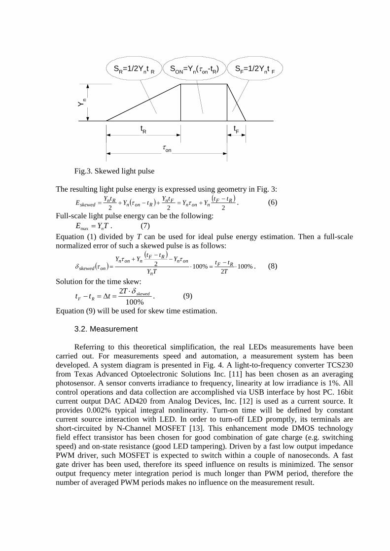
tR

on

tF

SR=1/2Ynt R SF=1/2Ynt FSON=Yn(on-tR)

Yn

Fig.3. Skewed light pulse

The resulting light pulse energy is expressed using geometry in Fig. 3:

222RF

nonnFn

RonnRn

skewedtt

YYtY

tYtY

E

. (6)

Full-scale light pulse energy can be the following: TYE nmax . (7)

Equation (1) divided by T can be used for ideal pulse energy estimation. Then a full-scale normalized error of such a skewed pulse is as follows:

%1002

%1002

T

tt

TY

Ytt

YYRF

n

onnRF

nonn

onskewed

. (8)

Solution for the time skew:

%100

2 skewedRF

Tttt

. (9)

Equation (9) will be used for skew time estimation. 3.2. Measurement Referring to this theoretical simplification, the real LEDs measurements have been

carried out. For measurements speed and automation, a measurement system has been developed. A system diagram is presented in Fig. 4. A light-to-frequency converter TCS230 from Texas Advanced Optoelectronic Solutions Inc. [11] has been chosen as an averaging photosensor. A sensor converts irradiance to frequency, linearity at low irradiance is 1%. All control operations and data collection are accomplished via USB interface by host PC. 16bit current output DAC AD420 from Analog Devices, Inc. [12] is used as a current source. It provides 0.002% typical integral nonlinearity. Turn-on time will be defined by constant current source interaction with LED. In order to turn-off LED promptly, its terminals are short-circuited by N-Channel MOSFET [13]. This enhancement mode DMOS technology field effect transistor has been chosen for good combination of gate charge (e.g. switching speed) and on-state resistance (good LED tampering). Driven by a fast low output impedance PWM driver, such MOSFET is expected to switch within a couple of nanoseconds. A fast gate driver has been used, therefore its speed influence on results is minimized. The sensor output frequency meter integration period is much longer than PWM period, therefore the number of averaged PWM periods makes no influence on the measurement result.

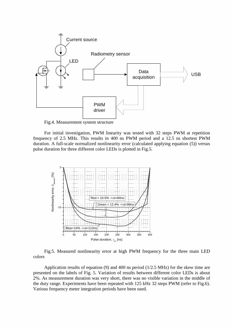
PWMdriver

Dataacquisition

LED

Radiometry sensor

Current source

USB

Fig.4. Measurement system structure

For initial investigation, PWM linearity was tested with 32 steps PWM at repetition

frequency of 2.5 MHz. This results in 400 ns PWM period and a 12.5 ns shortest PWM duration. A full-scale normalized nonlinearity error (calculated applying equation (5)) versus pulse duration for three different color LEDs is plotted in Fig.5.

0 50 100 150 200 250 300 350 400

-10

0

Blue=14% ->t=112ns

Green = 12.4% ->t=99ns

Red = 10.5% ->t=84ns

Non

linea

rity

erro

r,

skew

ed (

%)

Pulse duration, on

(ns)

Fig.5. Measured nonlinearity error at high PWM frequency for the three main LED

colors Application results of equation (9) and 400 ns period (1/2.5 MHz) for the skew time are

presented on the labels of Fig. 5. Variation of results between different color LEDs is about 2%. As measurement duration was very short, there was no visible variation in the middle of the duty range. Experiments have been repeated with 125 kHz 32 steps PWM (refer to Fig.6). Various frequency meter integration periods have been used.

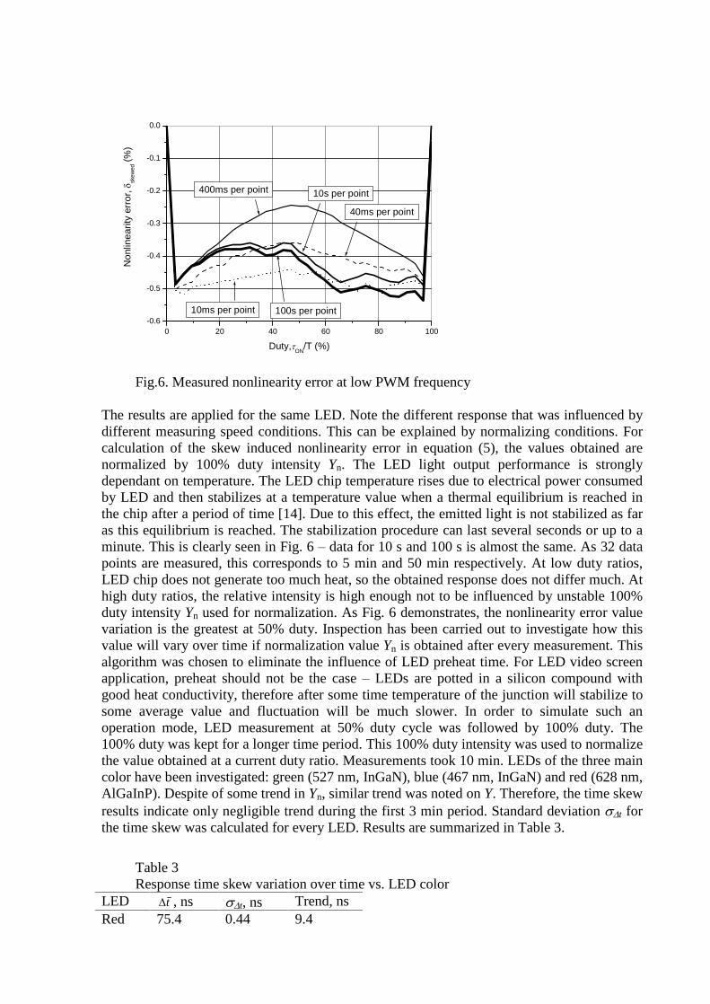
0 20 40 60 80 100-0.6

-0.5

-0.4

-0.3

-0.2

-0.1

0.0

100s per point10ms per point

400ms per point 10s per point

40ms per point

Non

linea

rity

erro

r,

skew

ed (

%)

Duty,ON

/T (%)

Fig.6. Measured nonlinearity error at low PWM frequency

The results are applied for the same LED. Note the different response that was influenced by different measuring speed conditions. This can be explained by normalizing conditions. For calculation of the skew induced nonlinearity error in equation (5), the values obtained are normalized by 100% duty intensity Yn. The LED light output performance is strongly dependant on temperature. The LED chip temperature rises due to electrical power consumed by LED and then stabilizes at a temperature value when a thermal equilibrium is reached in the chip after a period of time [14]. Due to this effect, the emitted light is not stabilized as far as this equilibrium is reached. The stabilization procedure can last several seconds or up to a minute. This is clearly seen in Fig. 6 � data for 10 s and 100 s is almost the same. As 32 data points are measured, this corresponds to 5 min and 50 min respectively. At low duty ratios, LED chip does not generate too much heat, so the obtained response does not differ much. At high duty ratios, the relative intensity is high enough not to be influenced by unstable 100% duty intensity Yn used for normalization. As Fig. 6 demonstrates, the nonlinearity error value variation is the greatest at 50% duty. Inspection has been carried out to investigate how this value will vary over time if normalization value Yn is obtained after every measurement. This algorithm was chosen to eliminate the influence of LED preheat time. For LED video screen application, preheat should not be the case � LEDs are potted in a silicon compound with good heat conductivity, therefore after some time temperature of the junction will stabilize to some average value and fluctuation will be much slower. In order to simulate such an operation mode, LED measurement at 50% duty cycle was followed by 100% duty. The 100% duty was kept for a longer time period. This 100% duty intensity was used to normalize the value obtained at a current duty ratio. Measurements took 10 min. LEDs of the three main color have been investigated: green (527 nm, InGaN), blue (467 nm, InGaN) and red (628 nm, AlGaInP). Despite of some trend in Yn, similar trend was noted on Y. Therefore, the time skew results indicate only negligible trend during the first 3 min period. Standard deviation t for the time skew was calculated for every LED. Results are summarized in Table 3.

Table 3 Response time skew variation over time vs. LED color

LED t , ns t, ns Trend, ns Red 75.4 0.44 9.4

Green 86.7 0.29 7.9 Blue 75.7 0.14 1.1

It should be noted that experiments indicate the stability of the error introduced by the skew. The next series of experiments carried out were using different LEDs from the same manufacturing lot. The results for blue LED are presented in Fig.7. In order to reduce preheat influence, same compensation was used. At every duty cycle, LED measurement was followed by 100% duty for normalization purposes. Note how flat the response (Fig.7) is now. In order to check for PWM duty change directionality influence (increasing or decreasing duty), an experiment has been carried out with increasing pulse duration (dashed line) and decreasing pulse duration (dotted line). No distinct difference between these two responses was observed.

0 200 400 600 800 1000 1200 1400 1600-110

-100

-90

-80

-70

Ske

w,

t (ns

)

Pulse duration, on

(ns)

Fig.7. Calculated skew time within one manufacturing lot for blue LED

In order to investigate how the experiment results for the skew time were distributed among three colors, Fig. 8 was generated. This figure indicates the count frequency for skew time t. The skew time was measured in the middle range of the duty cycle (400 ns to 1200 ns, refer to Fig. 7).

-110 -105 -100 -95 -90 -85 -80 -75 -70

Cou

nt (

a.u.

)

Skew, t (ns)

Red

-110 -100 -90 -80 -70

Cou

nt (

a.u.

) Green

-110 -105 -100 -95 -90 -85 -80 -75 -70

Cou

nt (

a.u.

) Blue

Fig.8. Skew time count frequency distribution for the main LED colors

It can be clearly seen that red color (AlGaInP) skew time t has smaller deviation. The averaging for one manufacturing lot has been performed in order to obtain some evaluation. The obtained results are summarized in Table 4. The time skew average is noted as t , whereas standard deviation as t.

Table 4 LED response time skew estimation within one manufacturing lot LED t , ns t, ns Red 74.7 1.1 Green 91.7 8.7 Blue 86.2 7.6

4. Results Application Usage of the estimated time skew value allows calculating PWM performance of any

period. Nonlinearity nonl due to light pulse skew can be calculated as a measured average intensity Ymeas error from expected intensity predicted by a current duty ratio, normalized by expected intensity:

%100

TY

TYY

onn

onnmeas

onnonl

. (10)

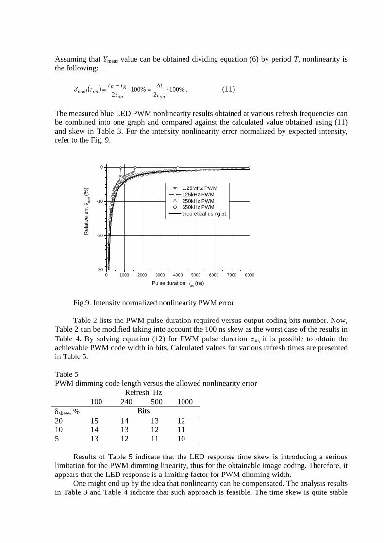
Assuming that Ymeas value can be obtained dividing equation (6) by period T, nonlinearity is the following:

%1002

%1002

onon

RFonnonl

ttt

. (11)

The measured blue LED PWM nonlinearity results obtained at various refresh frequencies can be combined into one graph and compared against the calculated value obtained using (11) and skew in Table 3. For the intensity nonlinearity error normalized by expected intensity, refer to the Fig. 9.

0 1000 2000 3000 4000 5000 6000 7000 8000-30

-20

-10

0

Rel

ativ

e er

r,

nonl (

%)

Pulse duration, on

(ns)

1.25MHz PWM 125kHz PWM 250kHz PWM 650kHz PWM theoretical using t

Fig.9. Intensity normalized nonlinearity PWM error Table 2 lists the PWM pulse duration required versus output coding bits number. Now,

Table 2 can be modified taking into account the 100 ns skew as the worst case of the results in Table 4. By solving equation (12) for PWM pulse duration on, it is possible to obtain the achievable PWM code width in bits. Calculated values for various refresh times are presented in Table 5.

Table 5 PWM dimming code length versus the allowed nonlinearity error Refresh, Hz 100 240 500 1000 skew, % Bits 20 15 14 13 12 10 14 13 12 11 5 13 12 11 10

Results of Table 5 indicate that the LED response time skew is introducing a serious

limitation for the PWM dimming linearity, thus for the obtainable image coding. Therefore, it appears that the LED response is a limiting factor for PWM dimming width.

One might end up by the idea that nonlinearity can be compensated. The analysis results in Table 3 and Table 4 indicate that such approach is feasible. The time skew is quite stable

both in time and within a manufacturing lot. Compensation can be carried out in the two following ways.

The simplest solution is to use driving pulse skew pre-compensation. For widening of analyzed LEDs, every PWM duty cycle by 100 ns will allow reducing nonlinearity, thus the number of available codes, almost for 10 times. Certainly, this will reduce the code availability at PWM cycle edges � close to 100% and close to 0%.

Applying a more complicated solution, the calibrated LED response may be used for codes selection. In this case, the codes may be applied more efficiently. However, usually more complicated PWM modulation algorithms are used [3, 15]. Such PWM modulation nonlinearity will have more complex response, therefore it should be studied for the artifacts indicated in this paper.

5. Conclusions A simple method for LED response time skew estimation was suggested. Using the

estimated skew, PWM dimming nonlinearity may be forecasted for various refresh frequency and code length combinations. It has been estimated, that the LED response time features the skew of approximately 100ns. This fact introduces nonlinearity for PWM dimming, when applied for LED video applications.

It has been indicated that 14 bits coding is a reasonable coding length, if 5% variation in image intensity is acceptable. An investigation, however, indicates that 14 bit PWM dimming is achievable only at refresh rates below 100 Hz. At desired refresh of 400 Hz, PWM dimming linearity within 5% is satisfied only by 11 bits code. This means that approximately 10% of input codes are above 5% accuracy if 2.4 gamma correction is used.

An experimental investigation demonstrates that the LED response time skew induced error is sufficiently stable and should allow the nonlinearity correction in order to apply the PWM pulse durations shorter than the indicated skew. In this case, code length can be increased. However, in order to evaluate this correction performance, a further study is needed.

Acknowledgement The author would like to thank Dr V.Dumbrava for a range of helpful discussions and

critical notes. References

[1] P.H. Putman, When Old is New Again, Videosystems (2002) pp.37-43 [2] E. F. Schubert, Light-Emitting Diodes, Cambridge University Press, 2003, p.313 [3] P.Narra, D.S. Zinger, An effective LED dimming approach, 39th IAS Annual Meeting, IEEE, 2004, pp.1671-1676 [4] C.A. Poynton, Gamma and Its Disguises, Journal of the Society of Motion Picture and Television Engineers, vol. 102, no. 12 (1993) 1099�1108. [5] Recommendation ITU-R BT.709, Basic Parameter Values for the HDTV Standard for the Studio and for International Programme Exchange, Geneva, ITU, 1990 [6] B.Wendler, Refresh rate, Technical note 42, Daktronics Inc., USA, 2002, p.1 [7] A.Descombres, W.Guggenbuhl, Large Signal Circuit Model for LED�s Used in Optical Communication, IEEE Trans. Electron Devices, vol. ED-28, no. 4, IEEE, (1981) 395-404 [8] I.Hino, K.Iwamoto, LED pulse response analysis considering the distributed CR constant in the peripheral junction, IEEE Trans. Electron Devices, vol.ED-26, no.8, (1979) 1238-1242

[9] M.Uhle, The influence of source impedance on the electrooptical switching behavior of LED�s, IEEE Trans. Electron Devices, vol.ED-23, no.4, (1976) 438-441 [10] R.Germer, Color LED flashes for stroboscopic videography, 25th International Congress on High-Speed Photography and Photonics, Beaune, France, 2002, pp.45-52 [11] TCS230 Programmable color light-to-frequency converter, datasheet TAOS046A, Texas Advanced Optoelectronic Solutions Inc., 2004, p.10 [12] AD420 Serial Input 16-Bit 4mA�20mA, 0mA�20mA DAC, datasheet rev.F, Analog Devices, Inc., 1999, p.11 [13] FDV301N Digital FET, N-Channel, datasheet FDV301N rev.F, Fairchild Semiconductor Corporation, 1999, p.5 [14] LED Metrology, Handbook of LED Metrology, Instrument Systems GmbH, 2000, p.40 [15] W D Howell, An overview of the electronic drive techniques for intensity control and colour mixing of low voltage light sources such as LEDs and LEPs. Application note 011 Artistic Licence Ltd, London, UK, 2002, p.9

Figure Legends Tables