a geotechnical, geochemical and human health risk
TRANSCRIPT

A Geotechnical, Geochemical and Human Health
Risk Assessment of a Dry Oil Lake Site in Kuwait
Humoud Melfi Zayed Aldaihani
A thesis submitted in partial fulfilment of the requirements for the
award of the degree of Doctor of Philosophy of the University of
Portsmouth
School of Civil Engineering and Surveying
University of Portsmouth
United Kingdom
January 2017

I
ABSTRACT
The main contribution of this study is to evaluate the effects of hydrocarbon contamination of
soil with respect to geotechnical and geochemical properties and their impact on human health
resulting from the Iraqi invasion of Kuwait in 1990. To fulfil this goal, the geotechnical and
geochemical characteristics of soil at a dry oil lake have been investigated.
The Human Health Risk Assessment (HHRA) was investigated utilising Risk Integrated
Software for Soil Clean-up Version-5 (RISC-5) to evaluate the effects of hydrocarbon
contamination on human health via ingestion of soil, dermal contact with soil, ingestion of
vegetables, inhalation of outdoor air and inhalation of particulates pathways.
In order to study these variations, two neighbouring sites at Al-Magwa area on the Greater
Burgan Oil Field were selected. The first was chosen for a dry oil lake scenario, and the other
adjacent site as an uncontaminated baseline control. Geotechnical tests were implemented on
samples taken at different depths from both sites. These included Atterberg Limit, Particle Size
Distribution (PSD), permeability and shear strength. Electronic micrographs were also taken
for the upper layer (0.0 m depth). The geochemical investigations included Hydrogen Ion
Concentration (pH), water soluble Chloride and Sulphate content, Vario Macro Elemental
Analysis (EA) and Gas Chromatograph Mass Spectrometry (GC-MS). GC-MS was carried out
to determine the specific hydrocarbon compounds and their concentrations within the soil.
These values formed the basis of a HHRA.
The geotechnical results show that hydrocarbon contamination modifies the PSD together with
a decrease in the angle of internal friction (φ). The geochemical results confirm that the
hydrocarbon contamination causes a change in the pH, with the Chloride and Sulphate contents
and hydrocarbon concentrations decreasing with depth. The HHRA demonstrated that certain
hydrocarbon compositions at elevated levels encountered in the dry oil lake site had potential
effects with regard to non-carcinogenic risks. The geotechnical and geochemical
characterisation data used in this study are also analysed quantitatively using IBM SPSS
Statistics in order to support robust results. The statistical analysis confirms that all the results
are solid and compatible.
Key words: Oil lakes; hydrocarbon contamination, geotechnical properties of hydrocarbon
contaminated soil; geochemical properties of hydrocarbon contaminated soil; human health
risk assessment.

II
TABLE OF CONTENTS
ABSTRACT…………………………...................................................................................I
TABLE OF CONTENTS……........................................................................................…II
DECLARATION..………………………………………………………………………..VI
LIST OF TABLES……………………………………………………………………...VII
LIST OF FIGURES…………………………………………………………………...…XI
LIST OF PLATES…………………….………………………………………….……XIX
GLOSSARY OF TERMS……………………………………………………………....XX
ACKNOWLEDGEMENTS………………………………………………………......XXII
DEDICATION………………………………………………………………….……XXIII
PUBLICATION............................................................................................................XXIV
1. INTRODUCTION……………………………..…………....…...…....1 1.1 Aim of the Study………………………………………..……………….…1
1.2 Background……………………………………………….……….……….2
1.3 Significance of the Study……………………………...……….…………..9
1.4 Scope of this Work………………………...……………………….…..…11
1.5 Structure of the Study…………………...…………………………….…12
2. CONTEXT OF THE STUDY: KUWAIT.…………………………14 2.1 Introduction……………………………………..……………………..…14
2.2 Kuwait Location………………………………………………..………...14
2.3 Kuwait Climate…………………………………………………………...16
2.4 Kuwait Solid Geology……………………..……………………………...17
2.4.1 Geology of Kuwait………..……………………….………….....17
2.4.2 Stratigraphy…..…………………...………..……..………….....22
2.4.3 Hydrogeology……………….……………..……...……….……29
2.5 Kuwait Superficial Geology………………...……………………………33
2.6 Degradation of Oil Lake Contamination in Kuwait….………..……….35
2.7 Kuwaiti Soil and Environmental Pollution…………………………..…36
2.8 Urban Expansion in the Contaminated Zone.….….…………………...45
2.9 Potential Human Health Risks from Hydrocarbon Contamination…..47
2.10 Summary…..…...……………………………………………………..….48
3. LITERATURE REVIEW………..………………………….….…...50 3.1 Introduction………………………………………………………….…...50
3.2 Overview of Hydrocarbon Contaminants………………………………52
3.3 Geotechnical Review of Soil Contaminated with Hydrocarbon.............58
3.3.1 Plasticity……….…………………………………………..........59
3.3.2 Particle Size Distribution (PSD)…………………………..........62
3.3.3 Scanning Electron Microscope (SEM)………………………...63
3.3.4 Permeability (Hydraulic Conductivity)…………...……………64
3.3.5 Shear Strength…………………………..……………….......…66
3.4 Geochemical Review of Soil Contaminated with Hydrocarbon.............68
3.4.1 Hydrogen Ion Concentration (pH)………………………..……69
3.4.2 Water Soluble Chloride (Cl-) and Sulphate (SO3 & SO4)
Contents…………………………………………………………72
3.4.3 Vario Macro Elemental Analysis (EA)…………………...……72

III
3.4.4 Gas Chromatograph Mass Spectrometry (GC-MS)…………....74
3.5 Human Health Risk Assessment (HHRA) of Hydrocarbon
Contaminated Soils…………………………………………...………..…79
3.5.1 Human Health Risk Assessment (HHRA) Scenarios…….……80
3.5.2 Human Health Risk Assessment (HHRA) Models……….........87
3.5.3 Risk Integrated Software for Soil Clean up (RISC) for
HHRA…………………………………………………………...93
3.5.4 Oil Contamination Risks on Human Health…………………..95
3.6 Summary……………………………………………………..…………...96
4. GREATER BURGAN OIL FIELD INVESTIGATION………….98 4.1 Introduction……………………………………………………………....98
4.2 Investigation Design………….…………………………………….…….99
4.3 Preliminarily Site Selection…………………………………..................104
4.3.1 Location of Greater Burgan Field (Al-Magwa Area)……..…106
4.3.2 Preliminary Assessment…………...………………...…...……108
4.3.3 Preliminary Soil Sampling…..…………...………………...…108
4.4 Final Selected Location (Greater Burgan Field-Al Magwa Area)…...109
4.4.1 Site Hazards and Restrictions........………………..........…….110
4.4.2 Site Safety Requirements……….…..……………...………….112
4.4.3 Site Walkover Survey………..…………………………..….…113
4.4.4 Site Description of Dry Oil Lake………...…………….……...114
4.5 Soil Sampling Plan and Strategy…….……………………...….............114
4.6 Sampling Methods for Potential Contaminated and Non-contaminated
Sites………………………………………………………………………119
4.6.1 Disturbed Sampling………………………………...…………122
4.6.2 Undisturbed Sampling……………………………...…………123
4.7 Soil Characterisation………………………………..…………..………128
4.7.1 Geotechnical Characterisation……………………………......129
4.7.1.1 Plasticity……………………........................................130
4.7.1.2 Particle Size Distribution (PSD)……………………...130
4.7.1.3 Scanning Electron Microscope (SEM)…………........130
4.7.1.4 Permeability (Hydraulic Conductivity)…….………...130
4.7.1.5 Shear Strength……...………………………..….………131
4.7.2 Geochemical Characterisation…………...…………….……..131
4.7.2.1 Hydrogen Ion Concentration (pH)…………………....132
4.7.2.2 Water Soluble Chloride (Cl-) and Sulphate (SO3 & SO4)
Content..………..……….………………………………..132
4.7.2.3 Vario Macro Elemental Analysis (EA)...……………..132
4.7.3 Hydrocarbon Characterisation……………………………..…133
4.7.3.1 Hydrocarbon Extraction……………………………..…133
4.7.3.2 Gas Chromatograph Mass Spectrometry (GC-MS)...137
4.7.3.3 Unresolved Complex Mixture (UCM)……….…….…139
4.8 Statistics Data Analysis…………..……………………………………...…141
4.8.1 Data Classification……………………………….................…141
4.8.2 Outlier Labelling Rule and Normality Tests……………….…143
4.8.3 Parametric and Non-Parametric Method……….……………144
4.8.3.1 T-Test……..…………………………………..…………..145
4.8.3.2 Mann-Whitney U Test……………………….…..……...145
4.8.3.3 Wilcoxon Signed Rank Test…………………..………..146
4.8.3.4 Regression Analysis …………………………………….146
4.8.4 Analysis Framework……………………………………..……147
4.9 Summary…………………………………………………………….…...148

IV
5. GEOTECHNICAL CHARACTERISATION…………………....149 5.1 Introduction…………………………………………….………….……149
5.2 Plasticity……..………………………………………………………..…149
5.3 Particle Size Distribution (PSD)……….…...……………………..……150
5.3.1 Laboratory Results of PSD……………………………………150
5.3.2 Statistical Summary of PSD…..…………...…………….……160
5.4 Scanning Electron Microscope (SEM)…..………………………..........173
5.5 Permeability (Hydraulic Conductivity)…..……..…………..…………177
5.5.1 Laboratory Results of Permeability………………….………..177
5.5.2 Statistical Summary of Permeability………………….………181
5.6 Shear Strength………..…………………….…………………….……..184
5.6.1 Laboratory Results of Shear Strength……………………...…184
5.6.2 Statistical Summary of Shear Strength…………………….…187
5.7 Summary……………………………………………………………..….192
6. GEOCHEMICAL CHARACTERISATION………...…….…..…194 6.1 Introduction…………….…………….…………………………………194
6.2 Hydrogen Ion Concentration (pH)…………...………………………...194
6.2.1 Laboratory Results of pH….……………………………..……194
6.2.2 Statistical Summary of pH……..………………………..…….199
6.3 Water Soluble Chloride (Cl-) and Sulphate (SO3 & SO4) Content….202
6.3.1 Laboratory Results of Cl-, SO3 and SO4 Content………….…202
6.3.2 Statistical Summary of Cl-, SO3 and SO4 Content……………207
6.4 Vario Macro Elemental Analysis (EA)………………………...............216
6.4.1 Laboratory Results of EA………………………..……………216
6.4.2 Statistical Summary of EA…..……………………...........……219
6.5 Gas Chromatograph Mass Spectrometry (GC-MS)…………...……...227
6.5.1 Laboratory Results of GC-MS…….…………………….…….227
6.5.2 Statistical Summary of GC-MS……………….………………237
6.5.3 Spatial Modelling of GC-MS Results (Contour Map)………..240
6.6 Summary……………………...…………………………………………247
7. HUMAN HEALTH RISK ASSESSMENT (HHRA) of
HYDROCARBON CONTAMINATED SOILS…………….……250 7.1 Introduction…………..…………………………………………………250
7.2 Human Health Risk Assessment (HHRA)…………………..…………251
7.3 Petroleum Hydrocarbon Standards for Soil Clean-up………….……252
7.4 Risk Assessment Stages (RAS)…………………..…………..…………259
7.4.1 Hazard Identification (phase 1a)..……………………….……260
7.4.2 Hazard Assessment (phase 1b)….…………………………….266 7.4.3 Risk Estimation (phase 2a)……………………………………268 7.4.4 Risk Evaluation (phase 2b)……………………………………271
7.5 Risk Assessment Stages Implementation on the Dry Oil Lake Site (Al-
Magwa Area)……………………...……………………………………..272
7.5.1 Hazard Identification (phase 1a)………………..…………….272
7.5.1.1 Site Definition and Description……………………………...272
7.5.1.2 Previous and Current Site Uses……………………………..273
7.5.1.3 Conceptual Site Model (CSM)……………………………….275
7.5.1.4 Initial Conceptual Site Model (CSM)……………………….275
7.5.2 Hazard Assessment (phase 1b)………….……………….……280
7.5.2.1 Hydrocarbon Contamination Detected in the Site……..…280
7.5.2.2 Hydrocarbon Contamination Exceed Screening
Value…………………………………………………………….286

V
7.5.2.3 Final Conceptual Site Model (CSM)………………………..286
7.5.3 Risk Estimation (phase 2a)……………………………………290
7.5.3.1 Routes Assessed Based on Final CSM and Parameters of the
Site Specific and Contaminants of Concern…..……..........290
7.5.3.2 Future Resident Receptor Parameters (Child and Adult)..295
7.5.4 Risk Evaluation (phase 2b)……………………………………298
7.5.4.1 Human Health Carcinogenic Risks…………………………298
7.5.4.2 Human Health Non-Carcinogenic Risks….………………..298
7.5.4.3 Site Specific Clean-up Level…………………………………298
7.6 Summary………………………………………………………………...307
8. DISCUSSION OF DEVELOPED SITE MODEL……………..…308 8.1 Introduction……………………………..………………………………308
8.2 Geotechnical Properties…..……..……………….……………………..309
8.2.1 Effect on Grain Size Distribution…………...………………...309
8.2.2 Effect on Permeability……………………………………...…310
8.2.3 Reduction in Angle of Internal Friction………………….…..310
8.3 Geochemical Properties…...……..……………………………….…….311
8.3.1 Change in the Acidity………………………………………….311
8.3.2 Effect on Chloride and Sulphate Content…………………….311
8.3.3 Changes in the Hydrocarbon Contamination with Depth…....312
8.4 Correlations in the Changes between Geotechnical and Geochemical
Properties………………………………………………………………..313
8.5 Human Health Risk Assessment (HHRA)…………….……………….315
8.5.1 Non-Carcinogenic Risks through Assumed Pathways….........315
8.5.2 Estimation of Clean-up Levels for the Dry Oil Lake…………316
9. FINAL CONCLUSIONS…………………………………………..317 9.1 General Overview…………………………………………………….…317
9.2 Geotechnical Properties……………..………………………………….317
9.3 Geochemical Properties………………………………………….……..318
9.4 Human Health Risk Assessment (HHRA)……………………………..319
10. FINAL RECOMMENDATIONS FOR FURTHER WORK…....320
REFERENCES……………………………………………..….………….322
APPENDICES (A, B, C & D) Attached in Enclosed Envelope (CD file).
APPENDIX A: 4. GREATER BURGAN OIL FIELD
INVESTIGATION……………………………………...350
APPENDIX B: 5. GEOTECHNICAL CHARACTERISATION……..392
APPENDIX C: 6. GEOCHEMICAL CHARACTERISATION………478
APPENDIX D: 7. HUMAN HEALTH RISK ASSESSMENT (HHRA) of
HYDROCARBON CONTAMINATED SOILS...........648

VI
DECLARATION
“Whilst registered as a candidate for the above degree, I have not been registered for any
other research award. The results and conclusion embodied in this thesis are the work of
the named candidate and have not been submitted for any other academic award”
Humoud Melfi Zayed Aldaihani.
Words Count: 63625 words (exclude references).
VII
LIST OF TABLES
Tables Titles Pages
Table 2.1. Surface stratigraphic classification and near-surface deposits in
Kuwait (Source: Al-Sulaimi & Mukhopadhyay, 2000)……………... 25
Table 2.2. Formations of the main oil producing reservoirs based on oil fields
locations in Kuwait……………………………………………………. 28
Table 2.3. The estimates of oil-polluted land areas and soil volumes in Kuwait
(Source: PEC, 1999)………………………………………………….. 43
Table 2.4. Some of the Mega Projects that are Under Construction (Source:
Almarshad, 2014, p. 49)………………………………………………. 46
Table 3.1. Classification of the Hydrocarbons…………………………………... 53
Table 3.2. Hydrocarbon fractions obtained from the distillation of crude oil
(TPH) (Source: Tomlinson et al., 2014)……………………………… 55
Table 3.3. Kuwait crude oil composition (Source: IARC, 1989)……………….. 56
Table 3.4. The pH classification in the soil (Source: Horneck et al., 2011)……. 70
Table 3.5. Summaries results of studies made by different researchers about
the changes in soil pH values due to crude oil contamination……… 70
Table 3.6. Examples of uncertainty factors utilised in chemical risk
assessment (Source: Hosford, 2009)………………………………….. 86
Table 3.7. Comparison between different model applications in the risk
assessment………………………………………………………...…… 89
Table 3.8. Limitations and suitability of various models in relation to Kuwait
conditions…………………………………………….………………… 90
Table 4.1. The Conditions utilised in ASE………………………………………. 135
Table 4.2. The method used in GC-MS instrument…………………………….. 137
Table 4.3. Number of soil samples utilised for the geotechnical tests………….. 142
Table 4.4. Number of soil samples utilised for the geochemical tests………….. 142
Table 4.5. Number of soil samples utilised for hydrocarbon pollutants
analysis test…………………………………………………………….. 142
Table 4.6. The tests used for parametric and non-parametric statistics
(Source: Pallant, 2005; Kasule, 2001)………………………………... 144
Table 5.1. Comparing mean values of soil classification constituents between
contaminated and non-contaminated samples at six different
depths of 0.0 m, 0.25 m, 0.5 m, 1.0 m, 1.5 m and 2.0 m……………... 156
Table 5.2. Mean value of the sieve analysis result for contaminated and non-
contaminated samples at six different of 0.0 m, 0.25 m, 0.5 m, 1.0
m, 1.5 m & 2.0 m)……………………………………………………...
157
VIII
Table 5.3. Indicates the significant differences of soil classification
constituents at six different depths between contaminated and non-
contaminated sites. (Note: outlier values were deleted in this
table)………………………………………………………………….... 164
Table 5.4. The significant differences of the Cu and Cc variables in the soil at
six different depths between contaminated and non-contaminated
sites. (Note: outlier vales were deleted in this table)………………… 171
Table 5.5. Mean value of the permeability coefficient (m/s) for contaminated
and non-contaminated samples at depths (0.0 m, 0.25 m, 0.5 m, 1.0
m, 1.5 m, 2.0 m) and its results via Hazen rule approximation….… 179
Table 5.6. The significant differences of the permeability coefficient (m/s)
variable in the soil at six different depths between contaminated
and non-contaminated sites…………………………………………... 182
Table 5.7. Comparing the mean values of the angle of internal friction (φ) for
contaminated and non-contaminated soil samples at six different
depths of 0.0 m, 0.25 m, 0.5 m, 1.0 m, 1.5 m and 2.0 m……………... 185
Table 5.8. The significant differences of the angle of internal friction (φ)
variable in the soil at six different depths between contaminated
and non-contaminated sites…………………………………………... 188
Table 6.1. pH coefficient values for the contaminated soil samples at six
different depths of 0.0 m, 0.25 m, 0.5 m, 1.0 m, 1.5 m and 2.0 m…... 196
Table 6.2. pH coefficient values for the non-contaminated soil samples at six
different depths of 0.0 m, 0.25 m, 0.5 m, 1.0 m, 1.5 m and 2.0 m….. 197
Table 6.3. Minimum, maximum and range of pH values in the soil at six
different depths for contaminated and non-contaminated sites……. 197
Table 6.4. The significant differences in the pH range variable in the soil at
six different depths between contaminated and non-contaminated
sites……………………………………………………………………... 200
Table 6.5. Mean values of water soluble chloride (Cl-) and sulphate (SO3 &
SO4) content (mg/kg) at different depths for the contaminated and
non-contaminated sites………………………………………………... 203
Table 6.6. The significant differences of the variables of Cl-, SO3 and SO4
concentration (mg/kg) in the soil at six different depths between
contaminated and non-contaminated sites. (Note: outlier values
were deleted in this table)……………………………………………..
210
IX
Table 6.7. Mean percentages values of Nitrogen, Carbon, Sulphur and
Hydrogen in soil samples at six different depths in contaminated
site……………………………………………………………………… 217
Table 6.8. Mean percentages values percentages of Nitrogen, Carbon,
Sulphur and Hydrogen in soil samples at two different depths (0.0
m, 0.25 m) in non-contaminated site…………………………………. 217
Table 6.9. The significant differences of the variables of elemental analysis (N
%, C %, H % & S %) at two different depths (0.0 m & 0.25 m)
between contaminated and non-contaminated sites (Note: outlier
values were deleted in this table)……………………………………... 222
Table 6.10. Number of detected and not detected samples with TPH tested by
GC-MS test at contaminated site…………………………………….. 230
Table 6.11. An example shows the results for one of the detected sample with
TPH which tested by GC-MS instrument for T.P.C (0 m, 25 m) at
depth (0.0 m) of contaminated site…………………………………… 231
Table 6.12. Mean values of the TPH concentration (mg/kg) in the soil samples
at contaminated and non-contaminated site at different depths…… 235
Table 6.13. The significant differences of the TPH variable in the soil between
different depths (0.0 m, 0.25 m & 0.5 m) at contaminated site…….. 238
Table 7.1. The 13 aromatic and aliphatic fractions with their leaching and
volatilisation (boiling point) that differ by approximately one order
(magnitude) (Source: TPHCWG, 1999)……………………………... 255
Table 7.2. The TPHCWG Petroleum Fractions (Source: Environment
Agency, 2003)………………………………………………………….. 256
Table 7.3. The main steps and their activities for phase 1a (Hazard
Identification) (Source: Nathanail et al., 2007)……………………… 261
Table 7.4. The main steps and their activities for phase 2a (Risk Estimation)
(Source: Nathanail et al., 2007)………………………………………. 269
Table 7.5. The Potential sources, pathways, intake route and receptors in the
contamination dry oil lake site (Al-Magwa area)…………..……..…
278
Table 7.6. The TPH fraction (aliphatic & aromatic), non-volatile chemical
substances (anthracene & phenanthrene related to PAH) and
unknown substances concentrations for the detected soil samples
found at dry oil lake in Greater Burgan Oil Field at depths (0.0 m,
0.25 m & 0.5 m)……………….……………………………………….. 282
Table 7.7. The 95 % Upper Confident Limit (UCL) of the mean value of
aliphatic & aromatic fractions and chemicals related to PAH
detected in Greater Burgan Oil Field (Al-Magwa area)……….…… 285
X
Table 7.8. Comparison between the mean value of 95 % UCL of the of TPH
concentration (mg/kg) in the site and the approved Screening
Value in the soil by U.S. EPA………………………………………… 286
Table 7.9. Final potential sources, pathways, intake route and receptors in
the contamination dry oil lake site (Al-Magwa area)…………...…... 288
Table 7.10. The selected exposure routes for HHRA in RISC-5 model based on
the hydrocarbon contamination located in the site…………………. 291
Table 7.11. Site specific parameters data measured and information of the
assumed pathway……………………………………………………… 292
Table 7.12. The properties of the chemical substances of concern as assumed
in RISC-5 software for contaminated located at unsaturated zone
soil pathway……………………………………………………………. 293
Table 7.13. Assumed specify exposure parameters of the future resident such
as Child and Adult receptors…………………………………………. 293
Table 7.14. Summaries the non-carcinogenic risk (HQ) results for child
resident from the contamination site (dry oil lake) based on
pathways assumed in the study site………………………………….. 302
Table 7.15. Summaries of non-carcinogenic risk (HQ) results for adult
resident from the contamination site (dry oil lake) based on
pathways assumed in the study site………………………………….. 303
Table 7.16. Comparing between the SSTLs (i.e. clean up levels) values and the
concentrations for the chemicals of concern detected in the site
(Greater Burgan Oil Field- Al Magwa area)………………………... 306
Table 8.1. Multiple regression (Backward elimination technique) predicting
TPH concentration (mg/kg) from fine sand %, curvature
coefficient (Cc), angle of internal friction (φ), SO4 (mg/kg) at
T.P.C. (50 m, 50 m)……………………………………………………. 314
XI
LIST OF FIGURES
Figures Titles Pages
Figure 2.1. Kuwait borders with adjacent countries (Source: Ezilon, 2015)….... 15
Figure 2.2. Major tectonic units of the Arabian Gulf region (Source: Al-
Sulaimi & Al-Ruwaih, 2004)………………………………………….. 18
Figure 2.3. The physiographic provinces of Kuwait (Source: Al-Sulaimi &
Mukhopadhyay, 2000)………………………………………………… 19
Figure 2.4. The geological map at the northern part of the Arabian Gulf region
(Source: Al- Sulaimi & Al-Ruwaih, 2004)…………………………… 21
Figure 2.5. The chronostratigraphy and lithology of Kuwait (Source: Carman,
1996)…………………………………………………………………… 23
Figure 2.6. Kuwaiti surface geological map (Source: Al-Sulaimi & Al-Ruwaih,
2004)……………………………………………………………………. 26
Figure 2.7. Hydrogeological and stratigraphy subdivision of the aquifer system
in Kuwait (Source: Mukhopadhyay et al., 1996)……………………. 30
Figure 2.8. Schematic representation of the hydrogeological system and
ground water flow in Kuwait (Source: Al-Rashed & Sherif, 2001, p.
779)……………………………………………………………………... 31
Figure 2.9. Groundwater fields location in Kuwait (Source: Bretzler, n.d., p.
3)………………………………………………………………………... 32
Figure 2.10. The mapping main indicators of land degradation in Kuwait
(Source: Al-Awadhi et al., 2005)……………………………………… 35
Figure 2.11. An oil well in flames in Kuwait during the Gulf war of 1991
(Source: Gay et al., 2010)……………………………………………... 37
Figure 2.12. A satellite captured this aerial view of the burning oil wells in
Burgan Field in Kuwait (A). Also, raging oil well fire burning
unrestrainedly in the Kuwait desert (B) and the environmental
damage caused by the fires and oil lakes which have had a lasting
impact on Kuwait’s ecosystem (C) (Source: KOC, n.d.)……………. 39
Figure 2.13. Oil trench in the north part of Kuwait (1999) showing different
levels and depths of oil contamination (Source: Al-Awadhi et al.,
2005)……………………………………………………………………. 41
Figure 2.14. An aerial view of the oil lakes formed as a result of the vandalism
inflicted by retreating forces (Source: KOC, n.d.)…………………... 42
Figure 2.15. Location of the Kuwait Oil Fields (Source: KMO, n.d.)……………. 43
Figure 3.1. Graphic clarification of the non-threshold and threshold toxicity
(Source: Hosford, 2009)……………………………………………….. 83

XII
Figure 4.1. Investigation design followed in this study…………………………... 101
Figure 4.2. Distance of the Greater Burgan Oil Field and the main residential
areas (Source: GM, n.d.)……………………………………………… 105
Figure 4.3. Oil lakes in Burgan Field (Source: Kaufman et al., 2000)…………... 106
Figure 4.4. The Greater Burgan sectors (Burgan, Al-Magwa & Al-Ahmadi
Fields) in Kuwait (Source: Kaufman et al., 2000)…………………… 107
Figure 4.5. Top view plan of Trial Pits (T.Ps) locations for soil samples at
potentially contaminated site in Greater Burgan Oil Field (Al-
Magwa area)…………………………………………………………… 116
Figure 4.6. Top view plan of Trial Pits (T.Ps) locations for soil samples at
potentially non-contaminated site in Greater Burgan Oil Field (Al-
Magwa area)…………………………………………………………… 117
Figure 4.7. Location of the potentially contaminated (dry oil lake) and non-
contaminated sites in Greater Burgan Oil Field (Al-Magwa
area)……………………………………………………………………. 118
Figure 4.8. Coordinates from GIS software for potentially contaminated
locations (dry oil lake site) at Al-Magwa area (A), dry oil lake
location that near to the GC-09 at Al-Magwa area (B) and the dry
oil contamination in soil at the site location (C)…………………...… 120
Figure 4.9. Coordinates from GIS software for potentially non-contaminated
site location at Al-Magwa area (A) Plus the non-contaminated Site
location that out of the Greater Burgan Oil Field fence (B) and one
of the trial pit located and desert plants in the site (C)……………... 121
Figure 4.10. Location of the sampling site and chemical laboratory at KISR
Ahmadi branch clarifying the distance between the two locations… 125
Figure 4.11. An example of an area under the peak of DRO……………………... 140
Figure 5.1. PSD curves for contaminated samples at depths (0.0 m, 0.5 m & 2.0
m)……………………………………………………………………….. 154
Figure 5.2. PSD curves for non-contaminated samples at depth (0.0 m, 0.5 m &
2.0 m)…………………………………………………………………… 155
Figure 5.3. Mean values of PSD for contaminated (brown colour) and non-
contaminated (green colour) samples at six different depths of 0.0
m, 0.25 m, 0.5 m, 1.0 m, 1.5 m and 2.0 m…………………………….. 158
Figure 5.4. Cu values of PSD in the soil for contaminated (brown colour) and
non-contaminated (green colour) samples at six different depths of
0.0 m, 0.25 m, 0.5 m, 1.0 m, 1.5 m and 2.0 m…………………………
159

XIII
Figure 5.5. Cc values of PSD in the soil for contaminated (brown colour) and
non-contaminated (green colour) samples at six different depths of
0.0 m, 0.25 m, 0.5 m, 1.0 m, 1.5 m and 2.0 m………………………… 159
Figure 5.6. Boxplots of silty/clay % (A), fine sand % (B) and medium sand %
(C) percentages values at six different depths for both
contaminated site and non-contaminated site. (Note: the symbol of
“*” and “°” in the graph denotes outlier)............................................... 162
Figure 5.7. Boxplots of coarse sand % (A), grave % (B) and exact soil-passing
No. #230 % (C) percentages values at six different depths for both
contaminated site and non-contaminated site. (Note: the symbol of
“*” and “°” in the graph denotes outlier)……………………………... 163
Figure 5.8. Comparing mean percentage values of exact soil passing sieve No.
#230 (A), fine sand (B), medium sand (C) and Coarse Sand (D) at
six different depths (in metres) between contaminated and non-
contaminated sites. (Note: Error bars denote standard deviation)…... 166
Figure 5.9. Comparing median percentage values of gravel at six different
depths (in metres) between contaminated and non-contaminated
sites. (Note: Error bars denote 95 % lower and upper confidence
intervals)………………………………………………………………... 167
Figure 5.10. Scatterplot of relationship between six different depths and
medium sand % values of T.P.C. (50 m, 50 m) at contaminated site
(A), and non-contaminated site (B)…………………………………... 168
Figure 5.11. Boxplots of uniformity coefficient (Cu) (A) and curvature
coefficient (Cc) (B) values at six different depths for contaminated
site and non-contaminated site. (Note: the symbol of “*” and “°” in
the graph denotes outlier)……………………………………………… 170
Figure 5.12. Comparing mean values of uniformity curvature (Cc) in the soil at
six different depths between contaminated and non-contaminated
site. (Note: Error bars denote standard deviation)……………………. 172
Figure 5.13. Comparing median values of uniformity coefficient (Cu) in the soil
at six different depths between contaminated and non-
contaminated site. (Note: Errors bars denote 95 % confidence
interval)………………………………………………………………… 172
Figure 5.14. A photograph enlarged by 20 times for soil sample taken from the
top soil of dry oil lake site at T.P.C (0 m, 100 m)…………..………... 174
Figure 5.15. A photograph enlarged by 20 times for soil sample taken from the
top soil of non-contaminated Site at T.P.C (0 m, 100 m)…………….
175

XIV
Figure 5.16. A photograph enlarged by 200 times for soil particles sample taken
from the top soil of contaminated (A) and non-contaminated site
(B) at T.P.C (0 m, 100 m) so that show the difference between these
sites……………………………………………………………………... 176
Figure 5.17. Comparison of the mean values of the permeability coefficient for
contaminated and non-contaminated samples at depths (0.0 m, 0.25
m, 0.5 m, 1.0 m, 1.5 m & 2.0 m) and the permeability coefficient
mean values via Hazen rule approximation…………………………. 180
Figure 5.18 Boxplots of permeability coefficient (m/s) values in the soil at six
different depths for contaminated site and non-contaminated site… 182
Figure 5.19. Comparing mean values of permeability coefficient (m/s) in the soil
at six different depths between contaminated and non-
contaminated site. (Note: Error bars denote standard deviation)......... 183
Figure 5.20. Comparing the mean values of the angle of internal friction (φ) for
contaminated (brown colour) and non-contaminated (green colour)
soil samples at six different depths of 0.0 m, 0.25 m, 0.5 m, 1.0 m,
1.5 m & 2.0 m…………………………………………………………... 186
Figure 5.21. Boxplots of angle of internal friction (φ) values in the soil at six
different depths for contaminated site and non-contaminated site… 188
Figure 5.22. Comparing mean values of the angle of internal friction (φ) in the
soil at six different depths between contaminated and non-
contaminated site. (Note: Error bars denote standard deviation)……. 189
Figure 5.23. Scatterplot showing relationship between six different depth
categories and angle of internal friction (φ) at T.P.C (50 m, 50 m),
at contaminated site (A) and non-contaminated site (B)……………. 191
Figure 6.1. Comparing range values of pH coefficient in the soil at six different
depths between contaminated and non-contaminated sites………… 198
Figure 6.2. Boxplots of pH values at six different depths for both contaminated
site and non-contaminated site. (Note: the symbol of “*” and “°” in
the graph denotes outlier)……………………………………………… 200
Figure 6.3. Comparing pH minimum and maximum values in the soil at six
different depths (in metres) between contaminated and non-
contaminated sites. (Note: the C and NC indicate to the
contaminated and non-contaminated site, respectively.)……………… 201
Figure 6.4. Comparing the mean values of the water soluble Chloride (Cl-)
content (mg/kg) in the soil at six different depths between
contaminated and non-contaminated sites…………………………...
204

XV
Figure 6.5. Comparing the mean values of the water soluble sulphate (SO3)
content (mg/kg) in the soil at six different depths between
contaminated and non-contaminated sites…………………………...
205
Figure 6.6. Comparing the mean values of the water soluble sulphate (SO4)
content (mg/kg) in the soil at six different depths between
contaminated and non-contaminated sites…………………………... 206
Figure 6.7. Boxplots of Cl- (A), SO3 (B) and SO4 (C) values in the soil at six
different depths for both contaminated and non-contaminated
sites. (Note: the symbol of “°” and “*” in the graph denotes outlier)... 209
Figure 6.8. Comparing median values of Cl- concentration (mg/kg) in the soil
at six different depths between contaminated and non-
contaminated site. (Note: Error bars denote 95 % lower and upper
confidence intervals)…………………………………………………… 211
Figure 6.9. Comparing mean values of SO3 concentration (mg/kg) in the soil at
six different depths between contaminated and non-contaminated
site. (Note: Error bars denote standard deviation)……………………. 211
Figure 6.10. Comparing mean values of SO4 concentration (mg/kg) in the soil at
six different depths between contaminated and non-contaminated
site. (Note: Error bars denote standard deviation)……………………. 212
Figure 6.11. Scatterplot showing relationship between six different depths and
SO3 concentration (mg/kg) at T.P.C (50 m, 50 m), at contaminated
site (A) and non-contaminated site (B)……………………………….. 214
Figure 6.12 Scatterplot showing relationship between six different depths and
SO4 concentration (mg/kg) at T.P.C (50 m, 50 m), at contaminated
site (A) and non-contaminated site (B)……………………………….. 215
Figure 6.13. Mean percentages values of carbon in soil samples at six different
depths in contaminated site…………………………………………… 218
Figure 6.14. Boxplots of N % (A) and C % (B) percentages values in the soil at
six different depths for contaminated site. (Note: the symbol of “*”
and “°” in the graph denotes outlier)………………………………….. 220
Figure 6.15. Boxplots of S % (A) and H % (B) percentages values in the soil at
six different depths for contaminated site. (Note: the symbol of “*”
and “°” in the graph denotes outlier)………………………………….. 221
Figure 6.16. Comparing mean values of N % (A), C % (B), S % (C) at two
different depths (i.e. 0.0 m, 0.25 m) between contaminated and non-
contaminated sites. (Note: Error bars denote standard deviation).......
223

XVI
Figure 6.17. Comparing median percentages values of H % at two different
depths (in metres) between contaminated and non-contaminated
sites. (Note: Error bars denote 95 % lower and upper confidence
intervals)………………………………………………………………...
224
Figure 6.18. Scatterplot showing relationship between six different depths and
N % (A), C % (B) and S % (C) percentages at T.P.C (50 m, 50 m),
at contaminated site…………………………………………………… 226
Figure 6.19. An example of Total Ion Chromatograms (TIC) of detected soil
sample with TPH for coordinate (0 m, 25 m) at depth (0.0 m), at
contaminated site (Al-Magwa area)……….…………………………. 232
Figure 6.20. Contour Map illustrated the top view of dry oil spilled in the soil at
depth 0.0 m in Greater Burgan Oil Field (Al-Magwa area)……...… 233
Figure 6.21. Contour map indicated the detected soil samples with TPH
concentration at depth 0.0 m in Greater Burgan Oil Field (Al-
Magwa area)…………………………………………………..……….. 234
Figure 6.22. Contour Map illustrated the top view of dry oil spilled in the soil at
depth 0.25 m in Greater Burgan Oil Field (Al-Magwa
area)……….............................................................................................. 236
Figure 6.23. Contour map indicated the detected soil samples with TPH
concentration at depth 0.25 m in Greater Burgan Oil Field (Al-
Magwa area)…………………………………………………………… 238
Figure 6.24. Contour Map illustrated the top view of dry oil spilled in the soil at
depth 0.5 m in Greater Burgan Oil Field (Al-Magwa
area)……….............................................................................................. 239
Figure 6.25. Contour map indicated the detected soil samples with TPH
concentration at depth 0.5 m in Greater Burgan Oil Field (Al-
Magwa area)…………………………………………………………… 241
Figure 6.26. Example of Chromatograph shows one of the non-detected samples
for the TPH tested by GC-MS instrument for T.P.C (0 m, 0 m) at
depth (0.0 m) of contaminated site…………………………………… 242
Figure 6.27. Example of Chromatograph shows one of the control sample tested
by GC-MS instrument for T.P.C (50 m, 50 m) at depth (0.0 m) of
control site……………………………………………………………… 243
Figure 6.28. Comparing the mean value of the TPH concentrations (mg/kg) in
the soil and depth at contaminated site………………………………. 244
Figure 6.29. Boxplots of TPH concentrations values (mg/kg) in the soil for
contaminated site. (Note: the symbol of “*” and “°” in the graph
denotes outlier)…………………………………………………………. 245

XVII
Figure 6.30. Comparing the median values of TPH concentration (mg/kg)
between different depths (i.e. 0.0 m, 0.25 m & 0.5 m) at
contaminated site. (Note: Error bars denote 95 % lower and upper
confidence intervals)……………………………………………………
246
Figure 7.1. Flowchart for the Hazard Identification (phase 1a) process
(Source: NHBC et al., 2008)…………………………………………... 262
Figure 7.2. An example of top view plan for some site as Conceptual Site
Model (CSM) part in phase 1a of risk assessment (Source: LQM,
2012)……………………………………………………………………. 263
Figure 7.3. An example of cross section for some site as Conceptual Site Model
(CSM) part in phase 1a of risk assessment (Source: LQM, 2012)….. 264
Figure 7.4. An example of network diagram for some site as Conceptual Site
Model (CSM) part in phase 1a of risk assessment (Source: LQM,
2012)……………………………………………………………………. 265
Figure 7.5. Flowchart for the Hazard Assessment (Phase 1b) process (Source:
NHBC et al., 2008)…………………………………………………….. 267
Figure 7.6. An example of potential exposure pathways of chemicals from
contaminated soils (Source: La Grega et al., 1994)………………….. 268
Figure 7.7. Flowchart for the Risk Estimation (phase 2a) process (Source:
NHBC et al., 2008)…………………………………………………….. 270
Figure 7.8. Flowchart for the Risk Evaluation (Phase 2b) process (Source:
NHBC et al., 2008)…………………………………………………….. 272
Figure 7.9. A previous photograph of the oil lake site obtained immediately
after the invasion in 1991 by media department at KOC…………... 273
Figure 7.10. A cross section for the Greater Burgan site (Al-Magwa area) as
initial Conceptual Site Model (CSM) in risk assessment…………… 277
Figure 7.11. Network diagram for dry oil lake site (Al-Magwa area) as
Conceptual Site Model (CSM) part in phase 1a of risk assessment... 279
Figure 7.12. An example of the Q-Q plot for TPH aliphatic EC12 - EC16 in dry
oil lake site (Al- Magwa area)……………..………………………….. 285
Figure 7.13. A cross section for the Greater Burgan site (al-Magwa area) as
Final Conceptual Site Model (CSM) in risk assessment…………….. 287
Figure 7.14. A network diagram for Greater Burgan oil site (Al-Magwa area) as
Final Conceptual Site Model (CSM) in risk assessment…………….. 289
Figure 7.15. The effect of the non-carcinogenic risks (HQ) on the children
receptor through exposure to hydrocarbon contamination via the
assumed routes in the study site…………………………………..…..
304

XVIII
Figure 7.16.
The effect of the non-carcinogenic risks (HQ) on the adult receptor
through exposure to hydrocarbon contamination via the assumed
routes in the study site…………………………………………………
305

XIX
LIST OF PLATES
Tables Titles Pages
Plate 4.1. Soil samples were stored within 18 °C temperatures before
transferring to the lab to be tested for Atterberg Limit, Sieve
Analysis, pH and Water soluble Chloride (Cl-) and Sulphate (SO3 &
SO4) contents……………….……………………………………………..
125
Plate 4.2. Dry oil lake at contaminated site (A), the works of digging at the
contaminated site (B) and the soil profile in the contaminated site
(C)…………………………………………………………………………
126
Plate 4.3. Non-contaminated soil samples (A) plus the undisturbed soil sample
taken for Direct Shear test at non-contaminated site (B) and the soil
Profile in the non-contaminated site (C)………………………………..
127
Plate 4.4. Accelerate Solvent Extractor (ASE-350) device used to extract the
hydrocarbon from the soil samples……………………………………...
135
Plate 4.5. Extract sample filtration (A) and the turbo evaporation system used
to concentrate the extract sample (B)…………………………………...
136
Plate 4.6. Agilent Technology 6890N GC with 5975B MSD and 7683B
Automatic Liquid Sampler………………………………………………
138
Plate 7.1. The oil wells pipelines nearby to the dry oil lake site (Al-Magwa
area)……………………………………………………..………………...
274
Plate 7.2. Dry oil lake site (Al-Magwa area)……………..………….…………….. 274

XX
GLOSSARY OF TERMS
AFCEE Air Force Centre for Environmental Excellence
ALARP As Low As Reasonably Practicable
ASE Accelerate Solvent Extraction
ASTM American Society for Testing and Materials
ATSDR Agency for Toxic Substances and Disease Registry
BISS Background Incremental Sample Simulator
BMD Benchmark Dose
BMR Benchmark Response
C Carbon
CADD Chronic Average Daily Dose
Cc Coefficient of Curvature
CH High Compressibility Clay
Cl- Chloride
CL Low Compressibility Clay
CLEA Contaminated Land Exposure Assessment
CO Carbon Monoxide
CO2 Carbon Dioxide
COPCs Constituents of Petroleum Concern
CR Carcinogenic Risk
CSM Conceptual Site Model
CTE Central Tendency Exposure
Cu Uniformity Coefficient
DEFRA Department for the Environment, Food and Rural Affairs
DNAPL Dense Non-Aqueous Phase Liquids
DQRA Detailed Quantitative Risk Assessment
DRO Diesel Range Oil
EA Elemental Analysis
EC Equivalent Carbon
ELCR Excess Lifetime Cancer Risk
EOD Explosive Ordnance Disposal
EPA Environment Protection Agency
GAC Generic Assessment Criteria.
GC Gas Centre
GCC Gulf Cooperation Council
GCI Green Cross International
GC-MS Gas Chromatograph Mass Spectrometry
GQRA Generic Quantitative Risk Assessment
H Hydrogen
HGG Hunting Geology and Geophysics
HHRA Human Health Risk Assessment
HI Hazard Index
HQ Hazard Quotient
HRA Health Risk Assessment
H2S Hydrogen Sulphide
HS&E Health Safety and Environment Department
IARC International Agency for Research on Cancer
KCCC Kuwait Cancer Control Center
KDP Kuwait Development Plan
KEPA Kuwait Environment Public Authority
KISR Kuwait Institute of Scientific Research
KMP3 Kuwait Master Plan
KOC Kuwait Oil Company
K-S Kolmogorov-Smirnoff
LNAPL Light Non-Aqueous Phase Liquid
XXI
LQM Land Quality Management
Mg/kg Milligrams Per Kilogram (=ppm)
MWs Monitoring wells
N Nitrogen
ND Non-Detect
NO Nitrogen Oxides
PAH Polycyclic Aromatic Hydrocarbon
Part IIA
Part IIA of the 1990 Environmental Protection Act (Part 2A in English
documents)
pH Hydrogen Ion Concentration
PO Production Operation Department
PPE Personal Protective Equipment
ppm parts per million
PSD Particle Size Distribution
Q-Q Quantile-Quantile
RAGS Risk Assessment Guidance for Superfund
RAS Risk Assessment Stages
RBCA Risk Based Corrective Action
RBSLs Risk Based Screening Levels
RfC Reference Concentrations
RfD Reference Doses
RISC-5 Risk Integrated Software for soil Clean-up-version 5
RME Reasonable Maximum Exposure
R&T Research and Technology Department
S Sulphur
SEM Scanning Electron Microscope
SGV Soil Guidelines Values
SM Very silty sand
S-M Silty sand (S-M)
SNIFFER Scottish and Northern Ireland Forum for Environmental Research
SO4 Sulphate
SO2 Sulphur Dioxide
SO3 Sulphur Trioxide
SP Poorly Graded Sand
SSAC Site Specific Assessment Criteria
SSTLs Site-Specific Target Levels
S-W Shapiro-Wilk
T.P Trial Pit
T.Ps Trial Pits
T.P.C Trial Pit Coordinate
T.P.Cs Trial Pit Coordinates
TPH Total Petroleum Hydrocarbon
TPHCWG Total Petroleum Hydrocarbon Criteria Working Group Series
TSEM Total solvent extraction material
UCLs Upper Confidence Limits
UCM Unresolved Complex Mixture
UoP University of Portsmouth
USEPA United States Environment Protection Agency
VOC Volatile Organic Compound

XXII
ACKNOWLEDGMENT
I would like to sincerely thank my first supervisor Dr. Paul Watson (School of Civil
Engineering and Surveying) for his continuous support and invaluable academic guidance
throughout the duration of the research. Similarly, Dr. David Giles (my second supervisor
from the School of Earth and Environment Sciences) who has been instrumental in
providing valuable technical support, particularly his support in the interpretation of
Human Health Risk Assessment and provided me with full knowledge concerning RISC-5
Software during the preparation of this thesis.
Also to the University of Portsmouth which provided me with all the necessary facilities,
resources, training courses and laboratories which have enabled me to carry out various
experiments and research.
My immense gratitude also goes to Dr. Musleh Alotaibi (Acting Manager of the production
operation at Kuwait Oil Company) and Eng. Eissa Aldaihani (Senior Reservoir Engineer at
Kuwait Oil Company) who have given me full accessibility and great facilities during
samples collection at Greater Burgan Oil Field. I would also like to thank Dr. Khaled Hadi
(Director/ Operations Division Water Research Center at Kuwait Institute for Scientific
Research (KISR)), who have supported me during the experimental phase by giving me the
permission to use the laboratories in order to carry out my research. Without the help of
these people, I would not have been able to complete my research. For that, I am eternally
indebted to them.
I especially thank my brother Dr. Sultan Melfi Aldaihani who sacrificed his time for
myself and provided me unconditional care and a close supervision. He always there when
I needed him. Dr. Sultan, with his a clear vision, always supported me and gave me
valuable advice in order to accomplish my mission in time. Special thanks for my mother,
my wife, my brothers and sister for their continuous support.

XXIII
DEDICATION
I dedicate this thesis to my late father (Melfi Zayed Aldaihani) who has always been my
source of inspiration. And also to my Mother, Wife, and all my Family Members whose
support have been my pillar of strength.

XXIV
PUBLICATION
Al-Daihani, H. M. Z., Watson, P. D. & Giles, D. P. (2014). A Geotechnical and
Geochemical Characterisation of Oil Fire Contaminated Soils in Kuwait. In G. Lollino
et al. (Eds.) Engineering Geology for Society and Territory, Vol. 6. Applied Geology for
Major Engineering Projects, 249-253. Springer.

1
1. INTRODUCTION
1.1 Aim of the Study
The central goal of this study is to investigate and determine whether the dry oil lake
contaminated soils in Kuwait have any influence on their geotechnical and geochemical
properties which could lead to a structurally unstable soil condition. This study will also
investigate the influence of dry oil lake on the Human Health Risk Assessments (HHRA)
and determine the potential levels of risk posed to any future urban developments within
the affected areas.
The main objectives with details are as follows:
(1) To study the geotechnical characteristics of hydrocarbon contaminated soil by
investigating whether dry oil lake residue can cause deterioration of soil geotechnical
conditions. This will be achieved by fulfilling the sub-objectives as set out below:
(a) to investigate the geotechnical properties of hydrocarbon contaminated soil;
(b) to investigate the geotechnical properties of non-contaminated (control) soil;
(c) to study the effect of dry oil lake residue on soil geotechnical properties by
comparing contaminated with non-contaminated samples.
(2) To study the geochemical characteristics of hydrocarbon contaminated soil, and to
test whether dry oil lake residue can create a chemically aggressive environment. This
will be achieved by answering the sub-objectives as set out below:
(a) by investigating the geochemical properties of hydrocarbon contaminated soil;
(b) by investigating the geochemical properties of non-contaminated (control) soil;

2
(c) by studying the effect of dry oil lake residue on the geochemical
properties of the soil to be achieved by comparing contaminated with non-
contaminated (control) samples.
(3) To assess the influence of the dry oil lake contaminated soils on the Human Health
Risk Assessment (HHRA) in the state of Kuwait from the existence of oil lake residue
since the Iraqi invasion in 1990. This will be accomplished by fulfilling the sub-
objectives as set out below:
(a) by classifying the pollutants in the hydrocarbon contaminated soils into
carcinogenic and non-carcinogenic categories; this will be achieved by
applying Risk Integrated Software for soil Clean-up (RISC-5) of the
hydrocarbon contaminated soil in Kuwait;
(b) by developing the „ground modelling‟ through obtaining the clean-up
level for the dry oil lake contaminated soil using RISC-5 software. Even if
the physical properties of the soil are suitable for construction purposes, it is
essential to carry out and to evaluate any signs of carcinogenic elements that
may influence the health of humans, animals and plants. The risk assessment
will be carried out using RISC-5 software, indicating that human health is
need addressing more than the strength of the soil.
1.2 Background
The impact on the environment - particularly towards public health and safety - due to
hydrocarbon contamination, can be catastrophic irrespective of contamination of the air
both above ground and below ground. As mentioned by Gay et al. (2010) and based on
other available reports, some of the most seriously hydrocarbon contaminated sites in the
world are: the Deepwater Horizon in the Gulf of Mexico; Northeast Ecuador; Exxon-

3
Valdezz in Alaska (U.S); Delta River in Nigeria; and Kuwait. According to Taylor et al.
(2005) the water and food consumed by individuals are the main causes of health affect
pollution. Humans and animals are not directly influenced by soil, however, water and
plants which are bonded to soil and used by humans and animals are directly affected by
contamination.
Thus the oil residue and heavy metal used in the war are likely to have resulted in the
contamination of the environment which will consequently have adverse impact on
people‟s health (Gay et al., 2010). Soil contamination is currently considered to be a vital
global issue; the main causes of soil contamination are human activities, some examples
being improper agricultural practices, faulty construction practices and industrial and
military activities. According to Goi et al. (2009) within the European Union alone, 3.5
million sites could have been contaminated of which 500 thousand sites needed
remediation. The emphasis of this study is on hydrocarbon contaminated soil present in
Kuwait caused by the burning of the oil wells as well as the release of huge volumes of oil
during the 1990 invasion by Iraq. During this war, approximately 604 oil wells were set
alight, oil gushed from 45 wells and 149 were severely damaged; in fact, two million
barrels of oil per day were estimated to have escaped from the affected wells (PAAC,
1999). In addition, it has been estimated that in 8 months 1.0 to 1.5 billion barrels of oil
were lost. As a result of these fires the Kuwait sky was covered with clouds of oil smoke.
When the fires were finally extinguished all the burnt oil landed on the ground and mixed
with the soil which is still contaminated to the present day (Petroleum Economist, 1992).
Based upon a report by (Green Cross International (GCI), 1998), the residue from large
(oil) lakes in particular, has been the cause of the main risk to the environment and to
human health as they have been left untreated.

4
This research will examine the hydrocarbon contaminated soil from the geotechnical,
geochemical and HHRA aspects since this hydrocarbon contamination might not only
affect the physical properties of the soil but the chemical risks are also likely to threaten
human health and the ecology.
A number of studies from various countries have investigated hydrocarbon contaminated
soil from the geotechnical perspective. These investigations have usually been undertaken
to examine the geotechnical properties of both contaminated and uncontaminated soil
samples typically by using the: Atterberg Limit test; Particle Size Distribution (PSD);
Scanning Electron Microscope (SEM); coefficient of permeability (Hydraulic
Conductivity); and the Direct Shear test.
The purpose of the Atterberg Limit test is to determine whether the plasticity of the soil has
changed due to the hydrocarbon contamination; the objective of PSD is to learn whether
change has taken place to the grain size due to hydrocarbon contamination. The SEM test
is used to further investigate the grain size distribution of the soil contaminated with
hydrocarbon in order to realise clearly whether there have been changes in the particles
from dry oil lake residue. The permeability coefficient (Hydraulic Conductivity) is utilised
to define the permeability of hydrocarbon contaminated soil and the Direct Shear test is
intended to determine any change in the internal friction angle (φ) and cohesion (c) of the
clean soil strength after being contaminated by hydrocarbon.
According to Caravaca and Roldan (2003), Meegoda and Ratnaweer (1995), Ijimdiya
(2013), and Srivastava and Pandey (1998), a number of studies have examined soil
contaminated by hydrocarbon using the PSD test while others have utilised the Atterberg
Limit Test to study soil plasticity including: Jia et al. (2011), Habib-ur-Rahman et al.
(2007), Shah et al. (2003), Patel (2011), Pandey and Bind (2014), and Elisha (2012). The
behaviour of the geotechnical characteristics of soil contaminated with hydrocarbon,
5
including Direct Shear and permeability coefficient (Hydraulic Conductivity), has been
examined by various studies including those of: Al-sanad (1995), Al-sanad and Ismael
(1997), and Khamehchiyan et al. (2007), Puri et al. (1994), Rahman et al. (2010), Gupta
and Srivastava (2010), Singh et al. (2009), Kermani and Ebadi (2012) and Shin et al.
(1999). However, Mucha and Trzcinski (2008), examined soil particles contaminated with
hydrocarbon using the SEM test so as to further investigate soil PSD (see section 3.3 for
further explanations).
Various nations have carried out a number of studies examining the geochemical properties
of hydrocarbon contaminated soil. Usually, the tests employed to examine the chemical
characteristics of the contaminated and uncontaminated soil were: Hydrogen Ion
concentration (pH); water soluble chloride (Cl-) and sulphates (i.e. sulphur trioxide (SO3)
& sulphate (SO4)); vairo macro elemental analysis (EA); and gas chromatography mass
spectrometry (GC-MS). The purpose of the pH coefficient test was to determine the acidity
or alkalinity of the soils either hydrocarbon contaminated or uncontaminated. Both water
soluble Cl- and SO3 & SO4 tests were performed to examine the suitability of the concrete
type to be utilised in construction projects on hydrocarbon contaminated sites. The vairo
macro elemental analysis (EA) test was aimed at examining the amount percentages (%) of
the chemical constituents (nitrogen (N %), hydrogen (H %), carbon (C %), and sulphur (S
%)) in hydrocarbon contaminated soil. The chemical composition and concentration of
total petroleum hydrocarbon (TPH) (mg/kg) was determined by using the GC-MS test.
Numerous studies examined the soils contaminated with hydrocarbon by identifying the
pH behaviour of both the uncontaminated and contaminated soils, see: Barua et al. (2011),
Khuraibet and Attar (1995) and Al-Duwaisan and Al-Naseem (2011). A study carried out
by others, including Onojake and Osuji (2012), examined the content of Cl- and SO3 &
SO4 within the soil. Yet other researchers carried out investigations to determine the

6
constituent percentages, for example: N (%); C (%); H (%); and S (%), in the hydrocarbon
contaminated soil by means of the Elemental Analysis (EA) test (Sato et al., 1997;
Perkinelmer, 2010; Benyahia et al., 2005). The concentrations of hydrocarbon
contaminants within soils as well as their chemical compositions have also been studied
with the help of GC-MS (see section 3.4 for detailed explanations).
Having looked at various works with regard to geotechnical and geochemical properties of
hydrocarbon contaminated soil, it has become apparent that some pollutants have been
amalgamated into the physical properties of the soil to become one of its constituents. As
these pollutants may become carcinogenic and pose a potential risk to the environment,
human and animal health could be severely affected. Additionally, a number of studies
available from the literature deal with carcinogenic pollutants found in hydrocarbon
contaminated soil. Certain particular mechanisms, scenarios and/or evaluations were
employed in these studies in an effort to classify and determine the level of risk towards
the surrounding environment from the carcinogenic pollutants.
Angehrn‟s (1998) study claims that it is essential to have a clear understanding of the
concentrations required and the methods used so as to move pollutants in the environment
from the hydrocarbon contaminated site to possible receptors. The usual procedure
employed in identifying and categorising risks to human health - as used by the U.S.
Environmental Protection Agency (U.S. EPA) are: Hazard Identification; Exposure
Pathways‟ Assessment; Toxicity Assessment; and Risk Characterisation (La Grega et al.,
1994).
Nathanail et al. (2007) have reported that the designed risk assessment was split into two
phases and two sub-phases, i.e. Phase 1a-Hazard Identification, Phase 1b-Hazard
Assessment, Phase 2a- Risk Estimation and Phase 2b-Risk Evaluation. These were
designed so as to evaluate the threats originating from the contaminated areas.
7
In order to identify the various chemical substances detected within the oil residue at
contaminated sites that could potentially affect health through the risk of exposure to
hazardous chemicals, Hazard Identification is usually employed (La Grega et al., 1994). A
method known as Exposure Pathways‟ Assessment is utilised to estimate the exposure to
certain chemicals by any environmental receptor likely to be at risk. This analysis is
necessary to ascertain how the hydrocarbon contaminants can be released from the site and
how migration of these contaminants to a possible receptor can be accomplished. La Grega
et al. (1994), have defined exposure pathways as follows by:
a contaminant source, e.g. landfill;
a chemical release mechanism, e.g. leaching;
a transport mechanism, e.g. groundwater flow;
an exposure point, e.g. well drinking water;
an environmental receptor, e.g. consumer of drinking water;
an exposure route, e.g., ingestion;
These examples must be existent to cause exposure.
According to La Grega et al. (1994), Toxicity Assessment offers toxicological data for the
relevant chemicals and/or predicted potential for adverse effects.
These assessments are derived from calculations of the physico-chemical properties of
chemicals combined with an integrated factor for safety. In other words, toxicity can be
described as a mixture of detrimental changes to biological organisms that might be
attributed to chemicals under certain circumstances - which can vary from minor changes
of normal functions to death (cancer) (Millner et al., 1992).
Risk Assessment, on the other hand, is employed to compare the effective concentrations
from exposure assessment against the accepted concentration derived from the toxicity
8
assessment. This approach allows for determination of the relative safety or risk associated
with the expected exposure (La Grega et al., 1994).
The evaluation of human health risk assessment of hydrocarbon contaminated soil has been
carried out by applying their scenarios as described in a number of studies including those
of Nathanail et al. (2007), Angerhn (1998), Hua et al. (2012), Dumitran and Onutu (2010),
Sarmiento et al. (2005), Iturbe et al. (2004), Irvine et al. (2014), Brewer et al. (2013) and
Bowers and Smith (2014).
On the other hand, other studies have carried out numerous models, e.g. Csoil,
Contaminated Land Exposure Assessment (CLEA), Risk Based Corrective Action
(RBCA), and RISC-4.02 which have been utilised in risk assessment aimed at evaluating
the concentration of carcinogenic and non-carcinogenic substances found in hydrocarbon
contaminated sites (Searl, 2012; GSI Environmental, 2014; Pinedo et al., 2012; Asharaf,
2011; Chen et al., 2004; Tomasko et al., 2001; Pinedo et al., 2014; Spence and Walden,
2001). Some authors have investigated diseases brought on as a result of hydrocarbon
contamination, for example, Amat-Bronnert et al. (2007), Campbell et al. (1993),
Ordinioha and Brisibe (2013) and Osman (1997) (section 3.5 for further clarification).
The aim of this research is to examine soil contaminated with hydrocarbon; this will be
carried out by means of RISC-5 assessment. The RICS-5 assessment includes a mixture of
procedural risk assessment which is limited only to: Exposure Pathway‟s Assessment,
Toxicity Assessment and Risk Characterisation which excludes Hazard Identification. The
software program is Windows based as it is capable of undertaking fate and transport
modelling, HHRA and ecological risk assessments for hydrocarbon contaminated sites. In
summary, it is intended to provide assessment of the potential adverse impacts to human
health (both carcinogenic and non-carcinogenic) for hydrocarbon contaminated sites
(Spence and Walden, 2001).

9
1.3 Significance of the Study
Based on the literature review in the previous section, it is noticeable that there is a high
tendency for hydrocarbon contaminated soil to affect the soil‟s geotechnical properties
which results in unstable soil conditions within its structure. Large hydrocarbon contents
within the soil tend to reduce the integrity of the soil properties resulting in defective
ground stability for any forthcoming development (Caravaca & Roldan, 2003; Meegoda &
Ratnaweer, 1995; Gupta & Srivastava, 2010; Pandey & Bind, 2014; Al-sanad et al., 1995;
Al-sanad & Ismael, 1997; Khamehchiyan et al., 2007).
Another concern is oil lake contamination which can affect the geochemical properties of
the soil creating a chemically aggressive atmosphere. Hydrocarbon chemical composition
present within sandy soil can potentially affect the soil‟s geochemical properties forming a
chemical composition that can have damaging effects on the environment (Barua et al.,
2011; Khuraibet & Attar, 1995; Al-Duwaisan & Al-Naseem, 2011; Onojake & Osuji, 2012;
Sato et al., 1997; Perkinelmer, 2010; Benyahia et al., 2005; Rahman et al., 2010).
The major issue related to hydrocarbon contaminated soil is that it can greatly affect
human health. Thus any proposed urban development planned in areas of concern can also
be affected. The fact that carcinogenic substances are present within these hydrocarbon
chemical compositions can cause an increase in respiratory diseases and cancer, e.g.
asthma and lung cancer (Angerhn, 1998; La Grega et al., 1994; Hua et al., 2012; Dumitran
& Onutu, 2010; Iturbe et al., 2004; Sarmiento et al., 2005; Irvine et al., 2014; GSI
Environmental, 2014; Brewer et al., 2013; Pinedo et al., 2012; Asharaf, 2011; Spence &
Walden, 2001).
The above issues, related to soil contaminated with oil lakes residue resulting from the
1991 Iraqi invasion of Kuwait, could create obstacles to future growth in construction
projects and urban development within the vicinity of the area of concern.
10
As demonstrated by Al-Sarawi et al. (1998b), the Kuwaiti Greater Burgan Oil Field
requires a detailed survey of the degree of contamination of the soil which is believed to be
as high as 80 %.This site was selected because it is not only highly polluted but also
because of its proximity to the metropolitan city since at any time in the near future,
development and construction projects are likely to take place. In any case there is an
urgent need to research and carry out a thorough exploration on the geotechnical and
geochemical properties of the Greater Burgan Oil Fields. To that effect, ground modelling
software RISC-5 should be used for risk assessment to human health. The area is highly
contaminated with hydrocarbon but the land is expected to be in high demand for future
developmental projects.
Furthermore, most of the research dealing with geotechnical and geochemical
characterisation of the hydrocarbon contaminated soil utilises soil which is artificially
contaminated by mixing virgin soil with various ratios of crude oil. To the best of author
knowledge, no detailed study has been dealt with the Kuwaiti hydrocarbon contaminated
soil after such long drying years of crude oil contamination.
Construction contaminated areas may include residential, commercial and healthcare
building projects. The key issue is that since the 1990 invasion by Iraq, approximately
49.13 km2 area of Kuwaiti land is covered with oil lakes (PEC, 1999). Most of the
hydrocarbon contaminated sites (oil lakes in particular) are close to residential areas which
the Kuwait Government plans to further develop. However, development should first take
contamination into consideration before any development in the hydrocarbon contaminated
sites takes place. Furthermore it is essential to assess the effect and risk of hydrocarbon
residue on human health and to estimate the possible levels of risk.

11
1.4 Scope of this Work
The focus of the experimental work for this study is centred on the geotechnical and
geochemical study of hydrocarbon contaminated soil and the way it could affect human
health. To achieve this, risk assessment will be carried out using ground modelling
software (RICS-5). The risk assessment will be developed and utilised as shown in Chapter
7.
To simplify the study, soil samples were obtained from two separate areas within the
Greater Burgan Oil Field at Al Magwa area; that is, from the contaminated site with dry oil
lake and also from a nearby site of soil before contamination. The latter being called the
non-contaminated site. The laboratory tests conducted were focused on the geotechnical
and geochemical properties, i.e. the physical, structural and chemical properties which
include the following:
(1) To ascertain the variation in physical properties of the hydrocarbon
contaminated soil performed by comparing samples taken from both
contaminated and non-contaminated areas, typically applying Sieve
Analysis test for PSD, SEM, Atterberg Limit and Constant Head
permeability tests.
(2) To ascertain the variation in Shear strength, (both contaminated and
non-contaminated soil samples were taken to perform a Direct Shear
test).
(3) To undertake chemical tests including the: pH coefficient; water
soluble Cl- and SO3 & SO4; EA and GC-MS; the aim was to ascertain:
the acidity or alkalinity; the suitability of concrete type to be utilised in
any future construction projects; the percentages of hydrogen, carbon,
nitrogen and sulphur as finger printing and hydrocarbon chemical

12
composition and their value in mg/kg of the oil polluted soil in both the
contaminated and non-contaminated sites.
The risk assessment on human health entails the use of the ground modelling method
known as RISC-5 software. The software was developed with the aim of classifying the
composition of hydrocarbon chemicals in the contaminated soil and the values in mg/kg.
1.5 Structure of the Study
This study comprises ten chapters showing the activities undertaken within the duration of
the work as follows:
Chapter 1- provides the aims and objectives of the study (as defined above), presents the
project background, identifies the importance of the study and outlines the scope of work
and how the study has been organised.
Chapter 2 - presents a study context within the state of Kuwait, with particular reference to
its location, climate, soil condition, geology, degradation of contaminated lands with oil
lakes, pollution to ground and environment, urban expansion due to construction and
human health risks from the 1991 oil lakes.
Chapter 3 – provides an overview of the hydrocarbon contaminants and covers a detailed
literature review of geotechnical and geochemical characterisations of the soils
contaminated by hydrocarbon residue and the affects on human health.
Chapter 4 - outlines the initial phases of the research programme identified as experimental
plan and phases, hazards and restriction, sampling plan and strategy, soil characterisation
and statistical data analysis.
Chapter 5 - illustrates the results of the laboratory tests with regard to geotechnical
characteristics of both contaminated and non-contaminated soils. This chapter also

13
discusses the main outcomes of the study demonstrating that the study aims have been
achieved by connecting the experimental findings with other studies found in the literature.
Chapter 6 - outlines the laboratory program associated with the geochemical properties of
the contaminated soil and hydrocarbon contaminated soil samples. Additionally, a
discussion on the main outcomes of the study and how the research objectives were
achieved using the experimental results linked with other studies in the literature.
Chapter 7 - describes Particulars of the HHRA scenarios which propose how to deal with
hydrocarbon residue contamination. The analysis and results of the ground modelling
development (RISC-5) software concerning human health and measuring the consequences
of Kuwait‟s dry oil lake contaminated soil on human health (the oil lake residue has
existed since 1990) are also provided.
Chapter 8 - focuses on interpretation of the results exhibited in Chapters five, six and seven
and the development of the understanding of the main research findings.
Chapter 9 - presents the final conclusion of the study.
Chapter 10- presents proposes recommendations for further work.

14
2. CONTEXT OF STUDY: KUWAIT
2.1 Introduction
This chapter aims to provide an introduction to: the location of Kuwait; assess and classify
the soil conditions; describe its climatic conditions; explain the geology; provide an
introduction and classification of the hydrocarbon contaminated lands; present descriptions
and clarification of the Soil and Environment Pollution; to investigate the risks from oil
spills on human health; and finally to report on the urban expansion of the construction
sector in Kuwait.
This means that a detailed description will be presented pertaining to Kuwait‟s location,
climatic conditions, ground conditions, geology, degradation of hydrocarbon contaminated
land, ground and environment pollution, urban growth of construction and risks to human
health due to residue of oil lakes.
2.2 Kuwait Location
Geographically, Kuwait is situated between latitude 28° 30' and 30
° 05' north of the
Equator and longitude 46' 30'' and 48' 30'' east of Greenwich; at the north-western corner of
the Arabian Gulf. It is a small country with an area of only 17,818 km2, (Murakami, 1995).
Iraq is situated on its north-west border and Saudi Arabia on its south and south- west
border (Figure 2.1 below).

15
Figure 2.1. Kuwait borders with adjacent countries (Source: Ezilon, 2015).
Due to its strategic location, Kuwait is regarded as one of the main gateways to the
Arabian Peninsula. The distance between the southern and northern most points of the
country is about 200 km (124 miles) while the eastern border is approximately 170 km
(106 miles) from the western border along latitude 29‟.
The total length of its borders - or the perimeter of the country - is around 685 km (426
miles), which includes 195 km (121 miles) at the eastern border facing the Arabian Gulf.
Therefore, 490 km (304 miles) is land frontier with 250 km (155 miles) fronting the
Kingdom of Saudi Arabia in the south/west and 240 km (149 miles) bordering the
Republic of Iraq in the north/west.
Study Area
16
2.3 Kuwait Climate
According to Nayfeh (1990), the climate of Kuwait can be described as arid, i.e. hot, dry
and lengthy summers with recurrences of dust phenomena and short, cold winters with
very little rain. Summer usually starts at the end of March and continues towards the end of
October. The true winter begins mid-December and usually ends towards mid-February.
Al-Kulaib (1984) claims that spring and autumn seasons are extremely short transitional
periods. The temperature differences between peak summer and winter is enormous; for
example, during summer, the long duration of direct sunshine onto the ground causes a
spiralling increase in temperature that can peak at 50 °C or higher in comparison with an
average monthly temperature of between 45 °C and 28 °C. The temperature during winter
through December and January, however, is exceptionally low; the average winter
temperature is between 21 °C and 8 °C. However, the lowest temperature may reach as low
as 0 °C or, at times, even lower. Kuwait receives a low annual rainfall of only 110 mm.
Another prevalent aspect of Kuwait‟s climate is the recurrence of dust storms; the dust
from the north west of the Arabian Gulf contributes to an annual deposit of 1 mm; similar
depositions take place along the whole coastal line. Additionally, there is a clear variation
in humidity which fluctuates from 60.9 % to 21.5 % from January to June. However,
depending on the season, there is also a high rate of evaporation which can vary from one
place to another with an average rate of 10.3 mm per day. Al-Jassar and Rao (2010, p.
4375), claim that the rate of evaporation varies in January and June from 4.6 mm/day to
22.9 mm/day respectively.

17
2.4 Kuwait Solid Geology
Kuwait‟s geological outline will be described in the following section. This will include
the rock structure which underlines Kuwait and also the aquifer‟s structural control. The
basic concerns are with the surface and sub-surface lithologies of the recent sediments. To
examine these areas more closely they will be divided into 3 sub-divisions, as follows: 1)
the surface geology of Kuwait; 2) the stratigraphy of Kuwait; 3) Kuwait‟s aquifer system.
2.4.1 Geology of Kuwait
The state of Kuwait is located at the north-eastern corner of the Arabian Plate between the
Precambrian shield to the west and the Zagros Fold belt towards the northeast. It is
bordered on the west and north by Iraq and on the south by Saudi Arabia (Figure 2.2).
As stated by Al-Sulaimi and Al-Ruwaih (2004), the state of Kuwait lies on three major
physiographic areas. A sequence of sedimentary rocks belonging to the Arabian platform
overlying the Precambrian Arabian Shield is present to the south and southwest.
The state of Kuwait lies on three major physiographic areas, i.e. a sequence of sedimentary
rocks belonging to the Arabian platform overlying the Precambrian Arabian Shield is
present to the south and southwest. These rocks of sedimentary outcrop are present within
a large belt along the eastern margin, which has less resistivity and has eroded to become a
series of low land strips. The Mesopotamian plain, with the Tigris and Euphrates Rivers‟
delta at the head of the Arabian Gulf, lies to the north-northwest of Kuwait while the
shallow marginal Arabian Gulf Sea which fences Kuwait lies to the east (Figure 2.2) (Al-
Sulaimi & Al-Ruwaih, 2004).

18
Figure 2.2. Major tectonic units of the Arabian Gulf region (Source: Al-Sulaimi & Al-
Ruwaih, 2004).
Kuwait Location

19
The topography of Kuwait can generally be described as monotonously flat with
moderately rolling plains separated by occasional scarps, small hills, valleys of ephemeral
streams and shallow wide inland depressions. Only in the Jal-Az-Zor small escarpment
along the north shore of Kuwait Bay Ahmadi Ridge paralleling the east coast of Kuwait
hills at Wara and Burgan, and the Wadi al Batin along the western border, is the local
relief not low (Al-Sulaimi & Al-Ruwaih, (2004)).
As shown in Figure 2.3, there are four physiographic provinces within the deserts of
Kuwait, i.e. i) Al-Dibdibba gravelly plain; ii) sand flat; iii) coastal flat; and iv) coastal hills.
Figure 2.3. The physiographic provinces of Kuwait (Source: Al-Sulaimi & Mukhopadhyay,
2000).
Al-Ahmadi
Ridge
Jal Az-Zor Hill
20
The surface and near surface geology of Kuwait has been dominantly controlled by the
Tertiary tectonic activity of the Arabian Plate. The northern and western sections of the
country lie within a huge previous outwash fan which expands far beyond the international
boundaries with Saudi Arabia and Iraq (Figure 2.4); this was originally deposited by a
watercourse, a precursor of Wadi Al-Batin and ending in Khor Al-Hammar in Iraq and the
northern coast of Kuwait Bay, it also extends well over the Dibdibba plain in Saudi Arabia
and Iraq. The slope to the north of Kuwait is continuous until broken by a shallow wide
inland depression caused by an inner drainage pattern (Umm Al-Aish, and Al-Raudhatain)
trailed by an extremely gentle dome-Shaped hill (reflection of the Sabriyah Raudhatain
Structures) controlling the watersheds (Al-Sulaimi & Al-Ruwaih, 2004).
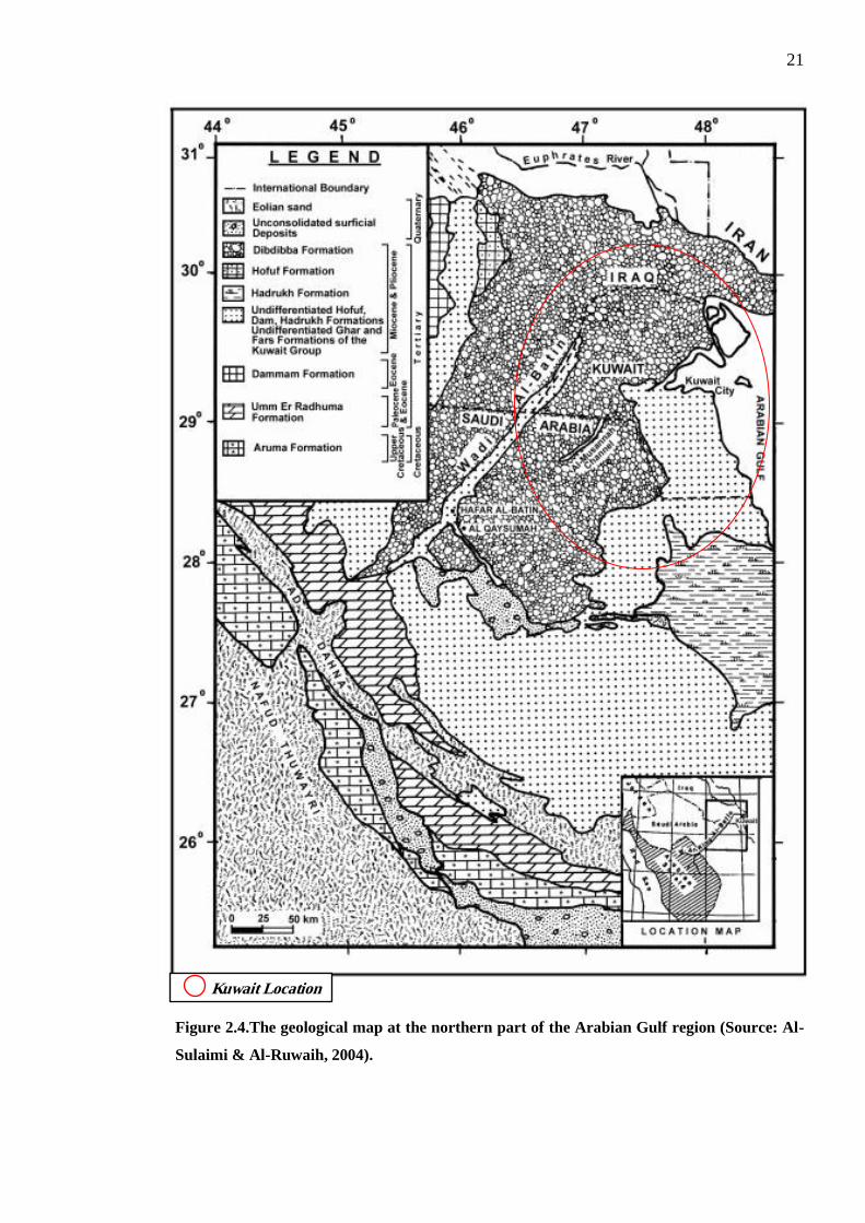
21
Figure 2.4.The geological map at the northern part of the Arabian Gulf region (Source: Al-
Sulaimi & Al-Ruwaih, 2004).
Kuwait Location
22
2.4.2 Stratigraphy
The Homocline of the Arabian Peninsula is part of Kuwait‟s interior and from the Miocene
to recent periods rocks have been exposed at the surface of this area - and throughout the
whole of Kuwait. However, because of the very „low dips and similarity of lithology‟ it
can be difficult to accurately correlate their formations; additionally, the accuracy of
tracing marker beds can only be sustained for a short while (Tanoli et al., 2015).
In accordance to Al-Sulaimi and Mukhopadhyay‟s (2000), the stratigraphy of the tertiary
succession of Kuwait can be generalised, (as illustrated in Figure 2.5). Kuwait‟s
Stratigraphy contains several groups, e.g. the Kuwait, Hasa, Aruma, Wasia, Thamama,
Riydh and Marrat groups - with each group being sub-divided into several formations.
However, for the purposes of this study, only the strata close to the surface – the Kuwait
and Hasa groups - will be dealt with in detail.
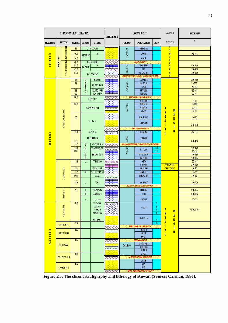
23
Figure 2.5. The chronostratigraphy and lithology of Kuwait (Source: Carman, 1996).
24
The Kuwait Group consists of the Dibdibba, Lower Fars and Ghar Formations (Table 2.1).
The Dibdibba Formation can be categorised into two groups, namely, the Lower Member
of the Mio-Pliocene age and the Upper Member of the Plio-Pleistocene age. Typically, the
former is comprised of very coarse grained, sandy and pebbly sandstone with a carbonate
cement. The latter constitutes gravelly sand and sandy gravel. The thickness of this
Dibdibba Formation is about 107 m (Al-Sulaimi & Mukhopadhyay, 2000; Al-Awadi et al.,
1997); while the lower Fars Formation is up to 350 m thick with a deposit of Lanhian–
Serravalian; it consists of evaporites interbedded with clastic red beds and carbonates of a
shallow marine environment (Al-Awadi et al., 1997). The Ghar Formation overlies the
Dammam Formation non-conformably and consists of sands and gravels with some rare
anhydrite, clays with the sandy limestone inter-bedded with a thickness of up to 274 m (Al-
Awadi et al., 1997).
The Hasa Group is comprised of Dammam, Rus and Umm Er-Radhuma Formations. The
Dammam Formation (middle to upper Eocene) - which varies in thickness from about 150
m in the southwest to about 275 m in the northeast - consists of a massive chalky
dolomicritic upper member, laminated biomicrites and domomicrites of the middle
member, and a nummulitic dense biomicritic lower member (Al-Sulaimi & Al-Ruwaih,
2004).
The Rus Formation (Lower-Middle Eocene) varies in thickness from 70-200 m and is
characterised by low porosity; the succession is made of limestone that is soft, carbonate
marly, gypsiferous plus minor sand and anhydrite (Al-Sulaimi & Al-Ruwaih, 2004). The
Emm Er-Radhuma Formation (Paleocene-Lower Eocene) non-conformably overlies the
Tayarat Formation of the Aruma Group. This Formation is encountered at depths of 164-
256 m in the southwest of Kuwait. The general lithology is made up of dolomite and
anhydrite, in places silicified and also intercalated with lignite.
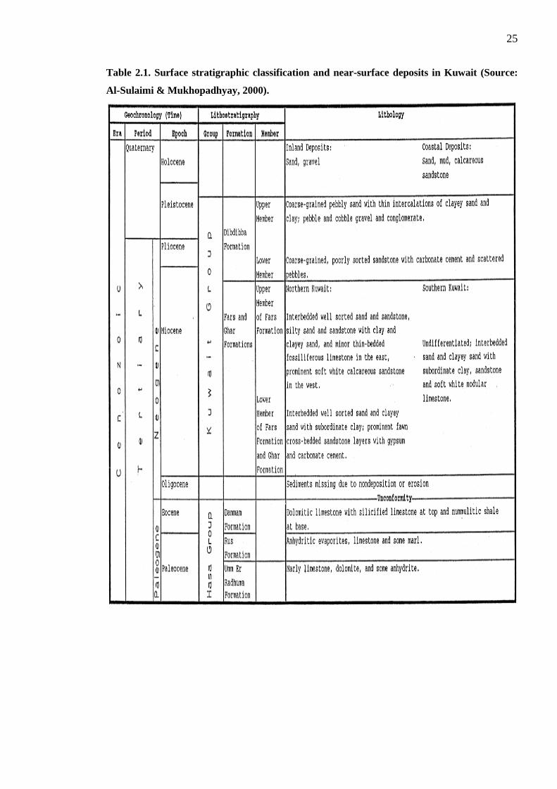
25
Table 2.1. Surface stratigraphic classification and near-surface deposits in Kuwait (Source:
Al-Sulaimi & Mukhopadhyay, 2000).
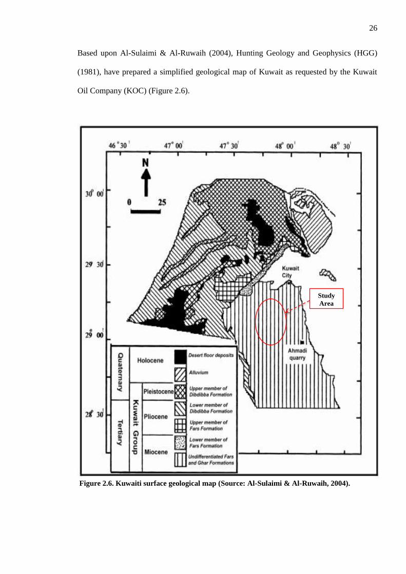
26
Based upon Al-Sulaimi & Al-Ruwaih (2004), Hunting Geology and Geophysics (HGG)
(1981), have prepared a simplified geological map of Kuwait as requested by the Kuwait
Oil Company (KOC) (Figure 2.6).
Figure 2.6. Kuwaiti surface geological map (Source: Al-Sulaimi & Al-Ruwaih, 2004).
Study
Area

27
The Dibdibba Formation gravels cover most of the area in northern Kuwait to the north
and northwest of Kuwait Bay. Additionally, the Dibdibba Formation - as shown in Figure
2.6 - is limited to the northern part of Kuwait. The Lower Fars fossiliferous equivalent
sediments do not extend to the north so the threefold subdivision of the clastic sediment
does not exist there. Therefore, the clastic sediments of the Kuwait Group are located at
southern part of Kuwait. They are classified as undifferentiated Ghar and Lower Fars. The
area chosen to be studied in this work is part of the Burgan oil lake which lies in the south
of Kuwait.
The formations of the main oil production areas in Kuwait differ from one location to
another. Table 2.2 shows the summary of all the reservoirs producing the majority of oil in
Kuwait.

28
Table 2.2. Formations of the main oil producing reservoirs based on oil fields locations in Kuwait.
Oil Field Name
Formations Names of the Main Oil
Producing Reservoir
Formations Periods References
Raudhatain Field
Ratawi, Zubair, Burgan and Mauddud
Formations.
Cretaceous.
(Carman, 1996).
Sabiriyah Field
Burgan, Mauddud and thin oil sands in the
Ratawi Formations.
Bahrah Field Burgan and Mauddud Formations.
Khashman Field Wara, Mauddud and Burgan Formations.
Greater Burgan Field Burgan, Mauddud and Wara Formations.
Minagish Field Burgan, Wara and Mishrif Formation/ Marrat,
Sargelul and Najmah Formations.
Cretaceous/ Jurrasic.
Abduliyah and Dharif Fields Marrat Formation. Jurrasic.
Umm Gudair Field Minagish Formation. Cretaceous. (Al-Khaled et al., 2012).
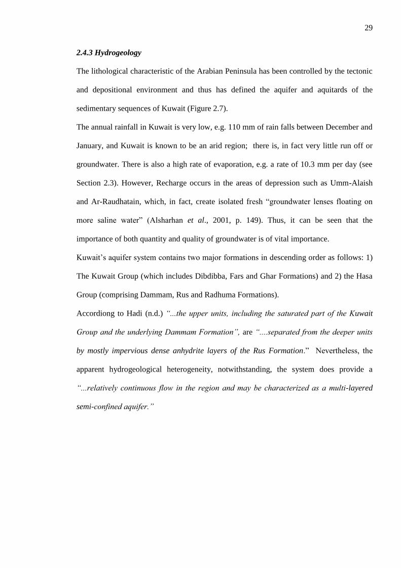
29
2.4.3 Hydrogeology
The lithological characteristic of the Arabian Peninsula has been controlled by the tectonic
and depositional environment and thus has defined the aquifer and aquitards of the
sedimentary sequences of Kuwait (Figure 2.7).
The annual rainfall in Kuwait is very low, e.g. 110 mm of rain falls between December and
January, and Kuwait is known to be an arid region; there is, in fact very little run off or
groundwater. There is also a high rate of evaporation, e.g. a rate of 10.3 mm per day (see
Section 2.3). However, Recharge occurs in the areas of depression such as Umm-Alaish
and Ar-Raudhatain, which, in fact, create isolated fresh “groundwater lenses floating on
more saline water” (Alsharhan et al., 2001, p. 149). Thus, it can be seen that the
importance of both quantity and quality of groundwater is of vital importance.
Kuwait‟s aquifer system contains two major formations in descending order as follows: 1)
The Kuwait Group (which includes Dibdibba, Fars and Ghar Formations) and 2) the Hasa
Group (comprising Dammam, Rus and Radhuma Formations).
Accordiong to Hadi (n.d.) “...the upper units, including the saturated part of the Kuwait
Group and the underlying Dammam Formation”, are “....separated from the deeper units
by mostly impervious dense anhydrite layers of the Rus Formation.” Nevertheless, the
apparent hydrogeological heterogeneity, notwithstanding, the system does provide a
“...relatively continuous flow in the region and may be characterized as a multi-layered
semi-confined aquifer.”
30
Figure 2.7. Hydrogeological and stratigraphy subdivision of the aquifer system in Kuwait
(Source: Mukhopadhyay et al., 1996).
Al-Rashed and Sherif (2001, p. 779) claim that the saturated sediments of the Kuwait
Group can be separated hydrogeologically into three units (Figure 2.8). These are known
as Upper Kuwait Group aquifer, A; Lower Kuwait Group aquifer, C; and Middle Kuwait
Group aquitard B. The former two have the capacity to store and transmit water, the latter
has low permeability bands and clayey lenses both of which, in combination, are used as

31
an aquitard for large areas of the city. Figure 2.8 shows the hydrogeological system and
groundwater flow in Kuwait.
According to Al-Rashed and Sherif (2001, p. 779) “...the phreatic conditions occur in the
upper unit of the Kuwait Group aquifer”. However, depending on the thickness of the low
permeable layers, the groundwater flow in the lower unit is subjected to semi-confined or
confined conditions, within both the Kuwait Group and the Dammam Formation. The
drainage system depends basically on the hydrogeological characteristics of the Kuwait
group with its interactions with the underlying units. Al-Rashed et al. (2010, p.108) specify
that the general flow of water in Kuwait comes from the southwest towards the northeast, it
then discharges into the Arabian Gulf Shatt Al-Arab.
Figure 2.8. Schematic representation of the hydrogeological system and ground water flow in
Kuwait (Source: Al-Rashed & Sherif, 2001, p. 779).
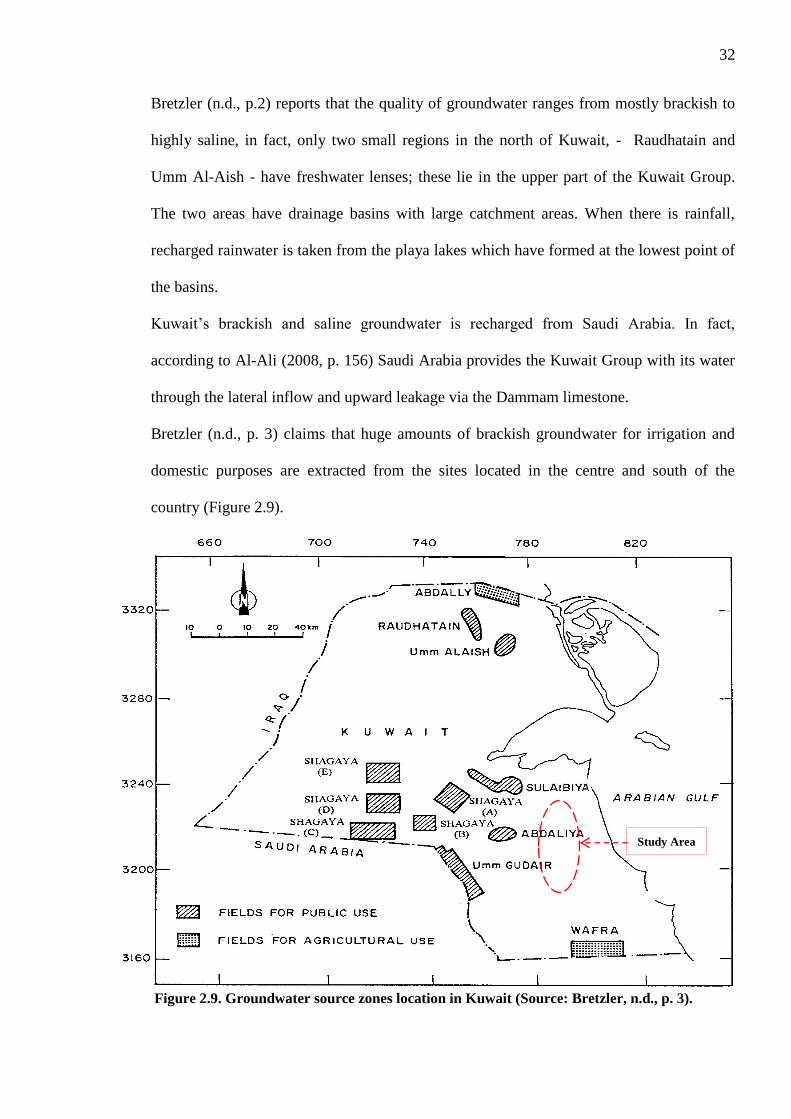
32
Bretzler (n.d., p.2) reports that the quality of groundwater ranges from mostly brackish to
highly saline, in fact, only two small regions in the north of Kuwait, - Raudhatain and
Umm Al-Aish - have freshwater lenses; these lie in the upper part of the Kuwait Group.
The two areas have drainage basins with large catchment areas. When there is rainfall,
recharged rainwater is taken from the playa lakes which have formed at the lowest point of
the basins.
Kuwait‟s brackish and saline groundwater is recharged from Saudi Arabia. In fact,
according to Al-Ali (2008, p. 156) Saudi Arabia provides the Kuwait Group with its water
through the lateral inflow and upward leakage via the Dammam limestone.
Bretzler (n.d., p. 3) claims that huge amounts of brackish groundwater for irrigation and
domestic purposes are extracted from the sites located in the centre and south of the
country (Figure 2.9).
Figure 2.9. Groundwater source zones location in Kuwait (Source: Bretzler, n.d., p. 3).
Study Area

33
This study is basically concerned with the soil contaminated with hydrocarbon located
close to the Kuwait oil fields. It is important, therefore, to investigate the ground water
depth near these oil fields in order to ascertain whether the hydrocarbon contamination
lakes, i.e. soil contaminated with crude oil, might also have migrated into the groundwater
if they are close to the ground surface. In fact, the depth of the groundwater in Kuwait
varies from one location to another.
To conclude, according to Al-Awadhi et al. (1992) and A1-Awadhi et al. (1993), the
ground water depths in Raudhatain and Sabriyah Oil Fields are approximately 30 m but the
Wafra Oil Field ground water depth is between 7 m to 20 m. No nearer surface aquifers
were observed in the Magwa, Ahamadi and Burgan Fields.
2.5 Kuwait Superficial Geology
As indicated by Nayfeh (1990), Kuwait, which lies at the north-eastern corner of the
Arabian Peninsula, is within the semi-arid zone. In general, the Arabian Peninsula can be
divided into two areas known as Arabian Shield and Arabian Shelf. The key components
of the former are igneous and metamorphic rocks belonging to the pre-Cambrian age
forming the western part of the peninsular. The latter controls the eastern section of the
peninsular consisting of thick sequences of terrestrial and shallow marine deposits, which
continue into Iraq and the Arabian Gulf along the north eastern border.
The Kuwait sedimentary sequence, which starts from the Middle Triassic to the modern
age, is over 6,700 m (20,000 feet) thick. Rocks and sediments belonging to the Eocene Age
extending to the modern age are the only remaining depositions left on the ground.
Dammam limestone (Eocene), the Kuwaiti Group of Sands, gravels and evaporate
(Micene-Pleistocene) are the rocks formed in the Eocene Age while the present deposits
consist of desert plain, eolian sand, playa, sabkha and beach deposits. According to Allison
(1969), the surface soil of Kuwait (including the majority of the Arabian Peninsula)

34
consists of fine to medium-grained, non-plastic, calcareous, wind-blown sands
accumulated in the area, with thicknesses of between 1m to 6 m - seldom exceeding 10 m.
Al-Sulaimi and Mukhopadhyay (2000) have stated that Kuwait is situated along the eastern
border of the deep sedimentary basin that forms the Arabian Peninsula, and is underlain by
fairly thick sedimentary rocks. Fairly undeveloped deposits belonging to the Dibdibba
Formation (Upper Miocene to Pleistocene Epochs, approximately 2 to 10 million years
old) extend above the surface. These deposits are further underlain by the Dammam
formation (Upper Eocene Epoch, approximately 38 to 42 million years old). With the
exception of Northern Kuwait, the intruding deposits which are usual feature from the Fars
Formation do not exist.
The Dibdibba Formation naturally consists of silica sands and gravels with inconsistent
amounts of silt and a few bands of thin clay and gypsum. Its cementation is comparatively
poor and incomplete, consisting of gypsum and calcium carbonate.
Currently, the Dibdibba Formation is overlain by deposits which consist of windblown
sand forming sheets and small sand dunes to the south of Kuwait. In general, calcareous
deposits are present adjacent to the coastline which commonly consist of oolithic and
bioclastic sands.
The amount of runoff discharging into the sea is small in view of the low seasonal rainfall
which mostly seeps into the ground or evaporates into the air. Evaporation has a very
dominant consequence on the normal groundwater movement pattern which is upward.
This occurrence results in the high concentration of soluble substances above the ground,
for example, gypsum and calcium carbonate. The prevailing materials obtainable close to
the ground surface in the northern and southern parts of Kuwait are calcium carbonates and
gypsum.

35
2.6 Degradation of Oil Lake Contamination in Kuwait
Soil contamination is considered one of the main environmental problems worldwide.
Undeniably, it originates from human activities such as unsuitable implementation of
agriculture, manufacturing, construction and military undertakings. An assessment by the
Goi et al., (2009, p.185) indicated that 3.5 million sites have been contaminated within just
the European Union. From this number, around 500,000 sites urgently require immediate
remediation in view of their levels of hydrocarbon contamination.
For an arid and dry country like Kuwait, the rate of land degradation can be accelerated by
the limited rain fall, water erosion and extreme wind conditions. Al-Awadhi et al. (2005)
claim that seven land degradation categories have been specified, as follows: erosion of
soil by water and/or wind; deteriorating quality of vegetation top soil; soil crusting and
sealing; soil compaction; oil pollution of soil; and soil salinisation (Figure 2.10).
Figure 2.10. The mapping main indicators of land degradation in Kuwait (Source: Al-Awadhi
et al., 2005).
Study Area

36
The landscape of Kuwait is specifically characterised by a number of depressions which
can easily contain dust and water throughout the year. Bashara (1991) realised that during
the Gulf War, at least 250 depressions or lakes of the natural landscapes were found to
contain crude oil spillage. Ground which has been severely contaminated has the potential
to pose risk to the quality of groundwater, aquifers and the inhabitants of the desert (Al-
Awadhi et al., 1992). Additionally, Amro (2004) claimed that the major causes of above-
ground and groundwater contamination was seepages of oil from oil wells, pipelines, gas
station storage tanks and the improper disposal of oil spills and petroleum waste.
Al-Awadhi et al. (2005) identified seven categories of land degradation occurring in
Kuwait which includes soil contamination caused by hydrocarbon. In this respect, the
author will endeavour to focus on oil lakes and soil pollution in an effort to assess the
consequences of such hydrocarbon contamination for land and ground (Section 2.7. for
explanation regarding oil lakes).
2.7 Kuwaiti Soil and Environment Pollution
Overall, the consequences of hydrocarbon contamination can be detrimental to the
environment particularly to the safety and health of mankind irrespective of whether it
takes place on the ground surface or below ground or indeed with ground water.
According to Taylor et al. (2005), the main sources of toxic pollution are from water and
food consumed by humans; additionally, Gay et al. (2010) claim that the oil or heavy metal
used in the war could potentially contaminate the environment causing severe effects on
human health.
As revealed by Seacor (1994) and others, the toxic could generated from the explosions
during the Gulf War contained heavy metal particulates and hydrocarbons. A number of
respiratory problem cases experienced by civilian and army personnel were reported
during the war, mainly due to the inhalation of toxic smoke (Smith et al., 2002). Based on
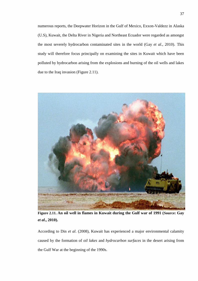
37
numerous reports, the Deepwater Horizon in the Gulf of Mexico, Exxon-Valdezz in Alaska
(U.S), Kuwait, the Delta River in Nigeria and Northeast Ecuador were regarded as amongst
the most severely hydrocarbon contaminated sites in the world (Gay et al., 2010). This
study will therefore focus principally on examining the sites in Kuwait which have been
polluted by hydrocarbon arising from the explosions and burning of the oil wells and lakes
due to the Iraq invasion (Figure 2.11).
Figure 2.11. An oil well in flames in Kuwait during the Gulf war of 1991 (Source: Gay
et al., 2010).
According to Din et al. (2008), Kuwait has experienced a major environmental calamity
caused by the formation of oil lakes and hydrocarbon surfaces in the desert arising from
the Gulf War at the beginning of the 1990s.

38
Al-Besharah (1991) stated that during the Gulf war, Kuwait‟s plain desert was covered
with major oil spillages owing to the burning and destruction of the oil wells. Five hundred
and sixty five oil wells were torched while 74 wells oozed uncontrollably from the ruined
wellheads (Figure 2.11 and 2.12). The oil field fires resulted in enormous black plumes of
smoke that finally settled as soot, tarmat and tarcrete deposits (El-Baz et al., 1994).
According to Seacor (1994), the scale of the plumes of smoke caused by the burning
wellheads was both remarkable and horrific; they stretched 22,000 feet above ground
covering 800 miles. Both soot and oil products, which had been partially burnt, were also
part of the smoke. In fact, Preston (2011) claimed that the smoke was also mixed with a
high content of carbon dioxide, sulphate and nitrogen.
The local environment was severely impacted by the catastrophe. In just nine months into
the incidence, over 60 million barrels of oil had been spilled from both the northern and
southern oil fields of Kuwait (Al-Saad, 1993). Furthermore, around 300 oil lakes (a total
area of over 49 km2) had been created within the northern and southern oil fields of Kuwait
(Al-Awadhi et al., 1996). On average, around 2 to 6 million barrels of oil were set ablaze
releasing a massive amount of sulphur dioxide and soot into the open air (Kwarteng &
Bader, 1993).
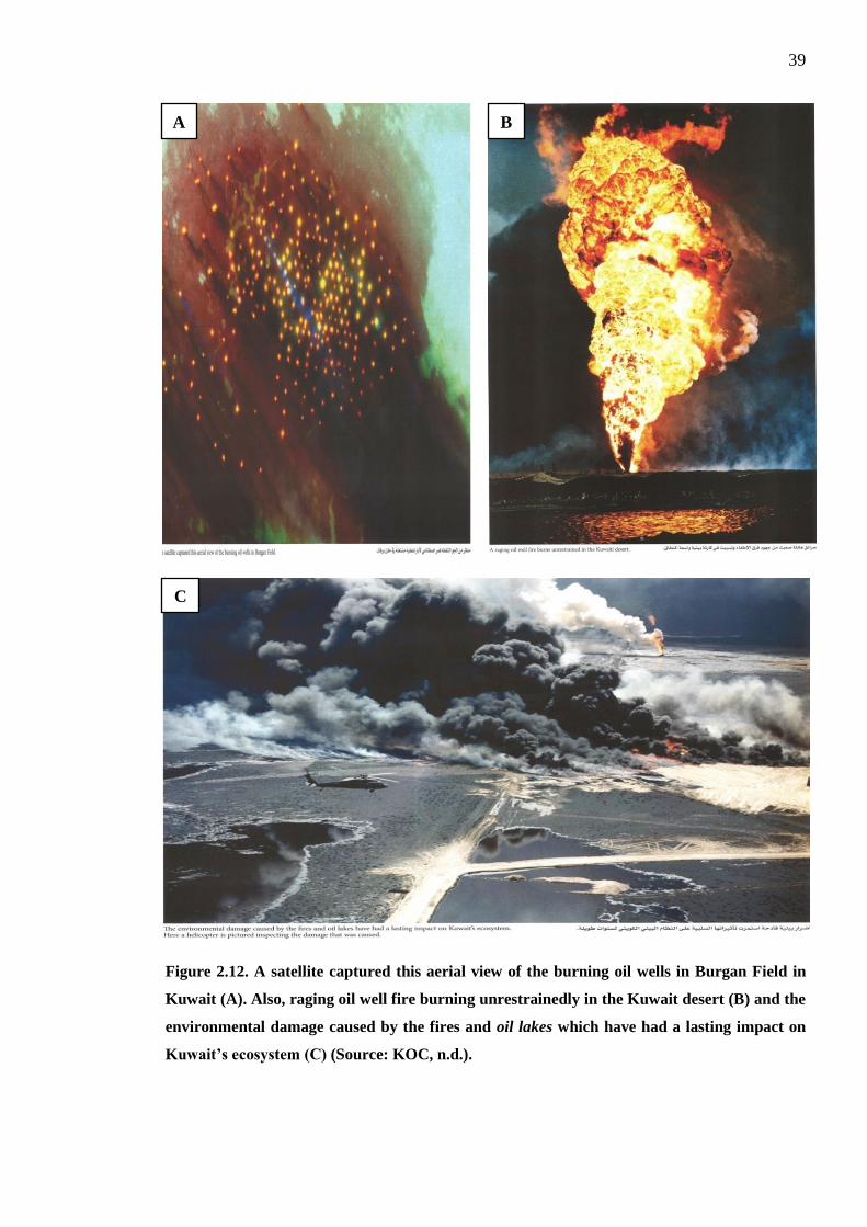
39
Figure 2.12. A satellite captured this aerial view of the burning oil wells in Burgan Field in
Kuwait (A). Also, raging oil well fire burning unrestrainedly in the Kuwait desert (B) and the
environmental damage caused by the fires and oil lakes which have had a lasting impact on
Kuwait’s ecosystem (C) (Source: KOC, n.d.).
A B
C

40
As a result of the uncontrolled and inexorable spillage of crude oil, oil lakes were formed.
Many researchers, including Al-Besharah et al. (1992), Al-Ajmi et al. (1994), El-Baz et al.
(1994), Salam (1996), Kwarteng (1998) and Al-Dousari (2001), have claimed that the
creation of these oil lakes has brought about an interest in detailed investigations as they
are unique; and considered to be one of the most disastrous environmental calamities of
modern times.
In Kuwait at present, three categories of terrestrial oil contamination have been defined,
these are:
(1) Oil lakes - described as build-ups of crude oil which has been
spilled from damaged well-heads and pipe routes in naturally low lying
grounds within the vicinity of the oil fields. According to Kwarteng
(1998) and Omar et al. (2000), currently, they can be divided into dry
and wet lakes.
(2) Tarcrete - defined as oil soot and oil mist which forms in the
surface layers of the soil as a 2-8 mm thick layer of unconsolidated soil.
It has been estimated that approximately 6 percent of the Kuwait land
area has been contaminated by tarcrete (Kwarteng, 1998).
(3) Oil trenches - consist of a part of the strategic hindrance systems
built during the war by the Iraqi army over a stretch of 220 m. They
include separate oil filled trenches of 4 - 5 m wide and 2 - 3 m deep
stretching along the boundary of southern Kuwait, approximately 10 -
14 km away from the Saudi Arabian border (Al-Ajmi et al., 1997).
Figure 2.13 shows the soil contamination at different depths and levels
in a trench in the northern area.

41
Figure 2.13. Oil trench in the north part of Kuwait (1999) showing different levels and depths
of oil contamination (Source: Al-Awadhi et al., 2005).
According to Al-Besharah and Salman (1991), the oil lakes were of various sizes and
shapes with depths that varied from a few centimetres to 1.5 meters (Figure 2.14).
Furthermore, the range of their original depths was between 0.05 m to 1.2 m with an
average depth of 0.3 m (Al-Awadhi et al., 1992; A1-Awadhi et al., 1993). Additionally, as
indicated by Al-Awadhi et al. (1992) and A1-Awadhi et al. (1993), the oil infiltrated into
the soil to a minimum depth of 0.4 m. These oil lakes were found in nine main oil fields of
Kuwait namely: Rawdhatain; Sabriyah; Ratga; Bahra Minagish; Umm Gudair and Wafra;
and the Greater Burgan Field (Ahmadi, Magwa, and Burgan Sectors) (Figure 2.15) (Cho et
al., 1997; Al-Duwaisan & Al-Naseem, 2011).

42
The largest hydrocarbon contamination occurred in the Burgan Field which constitutes 40
% of the overall contaminated volume (Al-Duwaisan & Al-Naseem, 2011). Based on the
assessment of pollution carried out in this area, the average penetration of oil into the soil
was one meter of which the surface 300 mm consisted of oily sludge which contained oil
penetration higher than 40 % (PEC, 1999). Massoud et al. (2000) claim that an
investigation into soil profiles in the concerned areas indicated that soil layers in a number
of places in Kuwait contained very high percentages of hydrocarbons - some up to a depth
of below 80 - 95 cm, in other sites up to 50 cm.
It was also discovered that a Gatch layer exists beneath these lowest points serving as a
moisture barrier preventing oil or water from penetrating further into the lower strata.
According to Al-Yaqout and Townsend (2004), this calcareous sand layer may be regarded
as linear in view of its low permeability. The Kuwait Oil Company (KOC) managed to
recover a significant volume of oil once the oil fires were extinguished (Hussain, 1995).
The remaining volume of oil which settled at the bed of the lakes however, is currently
considered to be irrecoverable (Saeed et al., 1995).

43
Figure 2.14. An aerial view of the oil lakes formed as a result of the vandalism inflicted by
retreating forces (Source: KOC, n.d.).
Figure 2.15. Location of the Kuwait oil fields (Source: KMO, n.d.).
Study Area

44
Table (2.3) below shows that the Burgan region has the largest area of oil pollution; the oil
polluted land area of the Burgan Oil Field is 25.6 km2 whereas the total of oil polluted
areas found in Kuwait is 49.13 km2.
Table 2.3. The estimates of oil-polluted land areas and soil volumes in Kuwait (Source: PEC,
1999).
Oil-polluted Soil Volume
(m2)
Oil-Polluted Area (Km2) Oil Field Region
1,956,000 3.26 Wafra
14,520,000 25.6 Burgan
95,000 0.19 Managish
135,000 0.27 Umm Gudair
2,456,000 12.28 Raudhatain
3,082,500 6.85 Sabryia
408,000 0.68 Bahra
22,652,500 49.13 Total
Balba et al. (1998), claim that the worst oil residue contaminated materials are located on
top of the oil lake bed which includes various items from stiff soil with a surface crust soil
to viscous tarry sludge, with a total petroleum hydrocarbon content of 133 g/kg and 694
g/kg respectively.
Kwarteng (1999) has stated that in 1998, the balance of area of oil lakes was reported to be
24.13 km2; in 2001 it was reported that the size of the oil lakes had not changed
(Kwarteng, 2001). Owing to the climatic conditions, a significant portion of these lakes
were concealed with dust and sand with the smaller oil lakes entirely covered, resulting in
an inability to detect original sizes and locations (Kwarteng, 1998).
The hot and arid climate of Kuwait (ambient summer temperature of 50 °C caused the
remaining oil in the majority of the lakes to thicken and become partly solid proving
difficult to remove. As pointed out by Saeed et al. (1998), the possible oil extraction from
the lake is estimated to weigh around 1.55 million tons. Continuing chemical tests of the
oil samples have revealed that the asphaltene, aromatic and resin contents have risen
45
because of the decrease in the quantity of volatile hydrocarbons and saturates (aliphatic
compounds) weathering has taken place (Saeed et al., 1998).
The prolonged decrease in volatile hydrocarbon from the oil surface has influenced the
creation of a de-volatilised viscous layer on the surface skin. According to Bufarsan et al.
(2002) and Barker and Burfarsan (2001), this skin layer has acted as a shield to the oil
layers below and results in a decrease in the overall evaporation rate. The properties of the
clean oil residue, which is water free, placed below the surface skin layer are comparable
to those of a typical medium crude residue with a boiling point of above 300° C indicating
that most of the light hydrocarbon within the oil has been lost (Khan et al., 1995).
Based on the numbers of oil lakes affected, the depths of the lakes and the oil
concentration and extent of areas affected, it has become clear that the extent of the soil
contaminated with hydrocarbon resulting from the Kuwait oil spills has been catastrophic.
Furthermore, since the Gulf War of 1991, the uncontrolled oil lakes have spread affecting
the soil below ground. Not only has the quality of the soil been affected as a result but this
hydrocarbon contamination has also caused changes in the chemical and physical
properties of the soil.
The Burgan Field is the largest contaminated oil lake as it constitutes 40 % of the overall
volume of the contamination (Al-Duwaisan and Al-Naseem, 2011, p.440). As such, it has
been selected as the case study for this research.
2.8 Urban Expansion in the Contaminated Zone
Due to the increase in the population one of the Kuwaiti government‟s key targets is the
provision of housing and the expansion of the residential homes‟ market. In fact, according
to the UK Foreign and Commonwealth Office (2014) a new five year development plan
(2015/2020) has been debated, approved and referred to Parliament by the Kuwaiti
Cabinet.
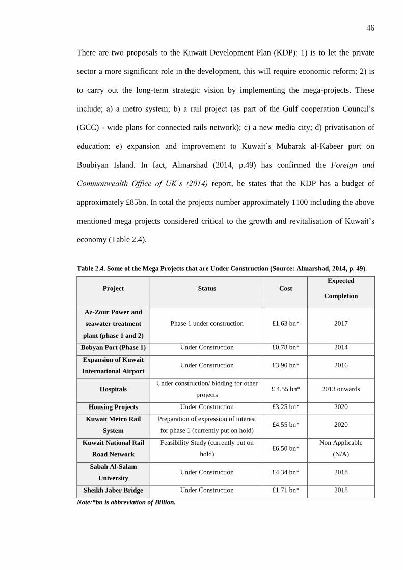
46
There are two proposals to the Kuwait Development Plan (KDP): 1) is to let the private
sector a more significant role in the development, this will require economic reform; 2) is
to carry out the long-term strategic vision by implementing the mega-projects. These
include; a) a metro system; b) a rail project (as part of the Gulf cooperation Council‟s
(GCC) - wide plans for connected rails network); c) a new media city; d) privatisation of
education; e) expansion and improvement to Kuwait‟s Mubarak al-Kabeer port on
Boubiyan Island. In fact, Almarshad (2014, p.49) has confirmed the Foreign and
Commonwealth Office of UK‟s (2014) report, he states that the KDP has a budget of
approximately £85bn. In total the projects number approximately 1100 including the above
mentioned mega projects considered critical to the growth and revitalisation of Kuwait‟s
economy (Table 2.4).
Table 2.4. Some of the Mega Projects that are Under Construction (Source: Almarshad, 2014, p. 49).
Project Status Cost
Expected
Completion
Az-Zour Power and
seawater treatment
plant (phase 1 and 2)
Phase 1 under construction £1.63 bn* 2017
Bobyan Port (Phase 1) Under Construction £0.78 bn* 2014
Expansion of Kuwait
International Airport Under Construction £3.90 bn* 2016
Hospitals Under construction/ bidding for other
projects £ 4.55 bn* 2013 onwards
Housing Projects Under Construction £3.25 bn* 2020
Kuwait Metro Rail
System
Preparation of expression of interest
for phase 1 (currently put on hold) £4.55 bn* 2020
Kuwait National Rail
Road Network
Feasibility Study (currently put on
hold) £6.50 bn*
Non Applicable
(N/A)
Sabah Al-Salam
University Under Construction £4.34 bn* 2018
Sheikh Jaber Bridge Under Construction £1.71 bn* 2018
Note:*bn is abbreviation of Billion.
47
As described and discussed above, the government of Kuwait has initiated a number of
mega projects planned to be developed from 2013 to 2020, These projects ignited my
interest in soil erosion and led to my undertaking further studies in soil contamination
through hydrocarbon in Kuwait. For the projects to succeed it is of the utmost importance
that investigation is carried out into the geotechnical and geochemical properties of the
hydrocarbon contaminated soils. The information learned can be utilised for construction
purposes; see sections 3.3 and 3.4 for detailed explanations regarding geotechnical and
geochemical characterisation of the soils contaminated with hydrocarbon.
2.9 Potential Human Health Risks from Hydrocarbon Contamination
During the break-out of the oil residue, one of the biggest concerns in Kuwait was the
possibility of health risks due to the emission of sulphur dioxide (SO2) and acid rainfall
(Al-Ajmi & Marmoush, 1996).
For decades it has been known that contaminated soil due to hydrocarbon and metal
contamination can affect humans causing environmental health risks (Certini et al., 2013).
As reported by Cho et al. (1997), the expansive nature of contaminated oil residue in the
Kuwaiti desert has caused an immense threat of contaminated subsurface water causing
detrimental effects on human health. The extent of contamination caused by
petrochemicals in Kuwait has, in fact, caused many health problems due to the different
range of exposure which can arise from the water, the land and the air (Abramson et al.,
2004). Due to the extensive nature of contamination by hydrocarbon, when the affected
area is ignited the crude oil becomes more dangerous and toxic as compared to its other
low sulphur substance (better known as sweet crude). As reported by Husain (1998),
contaminated soil can be detrimental to human health and can affect areas of vegetation
since burning oils emit huge amounts of toxic gasses including hydrogen sulphide (H2S),
carbon monoxide (CO), sulphur dioxide (SO2), oxides of nitrogen (NO(x)) and carbon

48
dioxide (CO2). Conditions are further exacerbated when the air is polluted by the partially
burned hydrocarbons and metals. The most common illnesses related to the Gulf War are:
respiratory problems; reproductive disorders; cancer risks; and psychological mood swings
(Gay et al., 2010). The identification of dangerous illnesses and diseases are associated
with soil contamination through hydrocarbon due to the 1991 Gulf War in Kuwait.
Due to the rise in such illnesses, it is paramount that the soil contaminated with
hydrocarbon be remediated so as to minimise the risks to human health, which is the focus
of this study. The study also seeks to investigate the extent to which soil contaminated with
hydrocarbon affects human health in general, e.g. illnesses such as cancer and respiratory
problems (Section 3.5).
2.10 Summary
Seven types of land degradation have already been identified and categorised including soil
contaminated by hydrocarbon (Al-Awadhi et al., 2005). This study will revolve around soil
contaminated with dry oil lakes (Section 2.7 for further elaboration).
This study examines the extent of contaminated soil caused by the dry oil lake in Kuwait
by investigating the hydrocarbon concentrations (mg/kg) under different depths and its
effects on geotechnical and geochemical properties of soil in this lake. It also examines the
extent of its adverse impact on human health since the Gulf War in 1991. In short the
study explores the quality of the soil affected by hydrocarbon contamination but also the
extent to which the soil might be altered in terms of its physical and chemical properties.
Due to the mega planning projects undertaken by the Kuwaiti government planned from
2013 to 2020, there is, in fact, an urgent need - for the purposes of construction - to
investigate geotechnical and geochemical properties of the soil polluted with hydrocarbon.
Studying the soil contaminated with hydrocarbon is crucial as Kuwait is embarking on an
expansion of its infrastructure with various mega constructions in the planning stage (See

49
sections 3.2 and 3.3 respectively for further clarification concerning the geotechnical and
geochemical characterisation of soil contaminated by hydrocarbon).
The preliminary findings of the study has encouraged the researcher to further probe into
the extent to which contaminated soil directly contributes to serious illnesses such as
respiratory problems, cancer risk, bronchitis etc. Therefore an investigation into the
dangerous illnesses and diseases resulting from soil contamination due to oil residue (Gulf
War 1991) will also be carried out. The increasing number of these illnesses gives rise to
an urgency to remediate the soil polluted with hydrocarbon in order to minimise the risks
to human health (Sections 3.5 for further explanations).

50
3. LITERATURE REVIEW
3.1 Introduction
Soil contamination with hydrocarbon is regarded as one of the key issues in Kuwait as the
oil spills from the oil wells has had a huge impact upon the virgin soil. In this respect, it is
vital for a study to be undertaken regarding the geotechnical and geochemical properties of
hydrocarbon contaminated soils in order that they can be used in environmental and
construction applications (Khamehchiyan et al., 2007). The migration of hydrocarbons
through the soil profile has the potential to affect the properties of the soil, e.g. Particle
Size Distribution, Moisture Content, Compaction, Shear Strength, Sulphate and Chloride
Content (Al-Sarawi et al., 1998b).
It is a key undertaking to investigate the geochemical properties of the soil contaminated
with oil lakes residue as petroleum hydrocarbon is a complex chemical which contains
organic composites; there are derived from a number of organic materials chemically
transformed over very long duration through varying geological environments. Oil is
mainly composed of hydrogen and carbon which contains a broad spectrum of
hydrocarbon sprightly gasses that will eventually transform themselves into heavy
residues. According to Wang et al., (1999), oil contains a small quantity of nitrogen,
sulphur and oxygen and metals such as iron, nickel and vanadium. Oil also comprises a
broad range of toxicities which can easily mix with soil which alters the soil‟s physical and
chemical properties (Barua et al., 2011). Oil will affect the population of microbes, plant
root systems and the oxygen content as soon as it penetrates any layer of soil. It should be
noted that soil which has been contaminated with hydrocarbon has inadequate properties to
allow plants to grow; this is mainly caused by the high level of toxic constituents present,
e.g. zinc and/or iron, and the reduction in the quantity of plant nutrients as a direct result of
the presence of toxins in the oil.
51
Discharges of petroleum hydrocarbons, in the past, into the soil environment can expose
human health, watercourses, ecosystems, properties and other receptors to potentially
serious threats. As mentioned by the Environment Agency (2003), it is vital to understand
the potential impacts of exposure to petroleum on each of these receptors. In order to
manage these risks research into this area will enable the development of a structured risk
assessment framework.
This chapter provides the information and parameters influencing the geotechnical and
geochemical classification of sandy soil contaminated with hydrocarbon. An introduction
will be given on the evidence and data of the oil residues and their impact on human health
so as to classify hydrocarbon contaminated Kuwaiti soil since the Gulf War (1990) - as
cited in previous studies whilst also recognising the limits of the studies.
An overview of the hydrocarbon contaminants is provided in section 3.2.The geotechnical
descriptions, i.e. strength and physical characterisations of sandy soils polluted with
hydrocarbon are explained in section 3.3. The geochemical investigation into soil
contaminated with hydrocarbon and the concentration of the hydrocarbon contaminant in
sandy soil is outlined in section 3.4. Former research explaining the potentially serious
effects of soil contaminated with oil residue and their risks to human health are presented
in section 3.5. The contribution of the literature review is provided in section 3.6; this
includes the agreed approach of this study taking into account some of the gaps identified
in earlier works.
52
3.2 Overview of Hydrocarbon Contaminants
In all forms, hydrocarbons are widely considered to be the most common contaminants to
be remediated in view of their prevalent existence and their potential threats to human
health and controlled waters (Churngold, n.d.).
According to (ATSDR, 1999), the term TPH is used to describe a large group of a few
hundred chemical compounds originating from crude oil. Crude oil is the basic ingredient
used in producing petroleum products with the potential to pollute the environment. In
view of the various chemicals present in crude oil, as well as other petroleum products, it is
impractical to carry out measurements on each chemical individually. Nonetheless, it is
beneficial to measure total amounts of TPH at contaminated sites (ATSDR, 1999).
Common types of fuel considered to be within the TPH family are: petrol; diesel; kerosene;
and lubricating oil/greases. Given the variety of compounds which consist of TPH and the
potential human health and environmental risks posed by them, the proposed remediation
techniques considered to control them ought to be taken into consideration based on the
actual site requirements (Baah, 2011).
According to Baah (2011), hydrocarbons consist of simple organic elements (containing
hydrogen and carbon), a number of different compounds are also available, each
compound displays various chemical and physical characteristics (Table 3.1).

53
Table 3.1. Classification of the Hydrocarbons.
Hydrocarbon
Classification
Hydrocarbon
Group Definition
Example of a
Hydrocarbon
Substance and
their Formula
References
Saturated
Hydrocarbon Alkanes
They are considered the simplest form of hydrocarbon
species made exclusively from individual bonds and are
saturated with hydrogen. For saturated hydrocarbon, their
general formula is CnH2n+2 (considering non-cyclic
structures). As the base of petroleum fuels, saturated
hydrocarbon can be present in the form of linear or
branched species. Hydrocarbon having similar molecular
formula however with different structure formula are
categorised as structural isomers.
Ethane
(C2H6)
(Silberberg, 2004)
Unsaturated
Hydrocarbon
Alkenes
These are hydrocarbons with single or multiple double or
triple bonds between carbon atoms. The hydrocarbons
with double bond are known as alkenes while
hydrocarbons which have single double bond have a
general formula of CnH2n (considering non-cyclic
structures).
Ethene
(C2H4)
Alkynes Alkynes are the term used for hydrocarbons with general
formula CnH2n-2 which contain triple bonds.
Ethyne
(C2H2)
Cycloalkanes Cycloalkanes
Hydrocarbon are formed when minimum of one carbon
ring is attached to hydrogen atmos. CnH2n is formulated
when a saturated hydrocarbon contains one ring.
Cyclopropane
(C3H6)
Aromatic
Hydrocarbon Arenes
Hydrocarbon have a minimum of one aromatic ring. Benzene
(C6H6)
54
In order to understand how TPH behaves when it is released into the atmosphere, it is
simplest to view the structure and size of the particular elements (Churngold, n.d.). TPH
mixtures having an aliphatic structure, i.e. straight or branched chains of carbon molecules,
will act in different ways to aromatic compounds (ringed chains of carbons). Likewise,
TPH mixtures with fewer molecules of carbon will also perform differently (Churngold,
n.d.).
Lighter ranges of TPH compounds (containing 16 carbon atoms or less) are likely to be
more mobile in view of their superior solubility, higher volatility and lower organic
partitioning coefficients. As indicated by Baah (2011), lightweight aromatic compounds,
for example benzene, tend to be highly toxic which can cause major threats in the event
that they escape into the environment. Compounds with heavier TPH usually have
contrasting characteristics in that they are likely to be adsorbed by the soil‟s organic
fraction. Aromatic compounds that are heavier, also known as Polycyclic Aromatic
Hydrocarbons (PAH), can be of higher toxicity and are generally highly obstinate in the
environment; according to (Baah, 2011), they usually exist in coal tar, heavy oils and
creosotes.
Tomlinson et al. (2014), have indicated that crude oil comprises a blend of linear,
branched, cyclic and aromatic hydrocarbons including asphaltenes and resins which have
high molecular mass components. Crude oil is distilled in refineries for the purpose of
separating the components into fractions characterised by having a common range of
boiling points (Table 3.2).

55
Table 3.2. Hydrocarbon fractions obtained from the distillation of crude oil (TPH) (Source:
Tomlinson et al., 2014).
Fraction Name Typical
Number of
Carbon
Atoms
Boiling Point
Range
(°C)
Uses (Examples)
Refinery Gas 3-4 < 30 Bottled Gas (propane or butane)
TPH-G 6-10 - Gasoline range organics
Petrol 6-10 100-150 Fuel for spark-ignition engines (e.g.,
cars,
motorbikes, vans)
TPH-D 12-28 - Diesel range organics
Naphtha 6-11 70-200 Solvents and used in petrol
Kerosene
(paraffin)
10-12 150-200 Fuel for jet engines and stoves
Diesel Oil 12-18 200-300 Fuel for compression ignition
engines (e.g.,
road vehicles, boats and trains)
Lubricating Oil 18-25 300-400 Lubricant for machinery
Fuel Oil 20-27 350-450 Fuel for ships and heating
Greases and
Wax
25-30 400-500 Lubricants and candles.
Bitumen >35 >500 Road surfacing
Most of the TPH mass partitioning will be carried out in the soil phase itself. In some
specific cases, it is also possible to find TPH in the form of phase separated liquid which
floats on the water-surface because of its buoyancy (ATSDR, 1999). Phase separated TPH
is usually termed Light Non-Aqueous Phase Liquid (LNAPL). A portion of TPH will turn
into liquid upon absorption by the groundwater or is stuck in the form of vapour in the soil
pores within the unsaturated area. In accordance with Churngold (n.d.), the actual
separation of phases is associated with the original source composition, hydrogeology and
geological conditions and the period since the spillage took place.
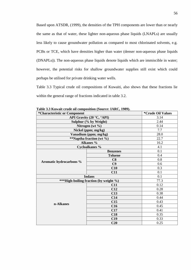
56
Based upon ATSDR, (1999), the densities of the TPH components are lower than or nearly
the same as that of water, these lighter non-aqueous phase liquids (LNAPLs) are usually
less likely to cause groundwater pollution as compared to most chlorinated solvents, e.g.
PCBs or TCE, which have densities higher than water (denser non-aqueous phase liquids
(DNAPLs)). The non-aqueous phase liquids denote liquids which are immiscible in water;
however, the potential risks for shallow groundwater supplies still exist which could
perhaps be utilised for private drinking water wells.
Table 3.3 Typical crude oil compositions of Kuwaiti, also shows that these fractions lie
within the general range of fractions indicated in table 3.2.
Table 3.3 Kuwait crude oil composition (Source: IARC, 1989).
*Characteristic or Component *Crude Oil Values
API Gravity (20 °C, °API) 3.14
Sulphur (% by Weight) 2.44
Nitrogen (wt %) 0.14
Nickel (ppm; mg/kg) 7.7
Vanadium (ppm; mg/kg) 28.0
**Naptha fraction (wt %) 22.7
Alkanes % 16.2
Cycloalkanes % 4.1
Aromatic hydrocarbons %
Benzenes 0.1
Toluene 0.4
C8 0.8
C9 0.6
C10 0.3
C11 0.1
Indans 0.1
***High-boiling fraction (by weight %) 77.3
n-Alkanes
C11 0.12
C12 0.28
C13 0.38
C14 0.44
C15 0.43
C16 0.45
C17 0.41
C18 0.35
C19 0.33
C20 0.25

57
Table 3.3. Continuous (Source: IARC, 1989).
*Characteristic or Component *Crude Oil Values
n-Alkanes
C21 0.20
C22 0.17
C23 0.15
C24 0.12
C25 0.10
C26 0.09
C27 0.06
C28 0.06
C29 0.05
C30 0.07
C31 0.06
C32 plus 0.06
Iso-alkanes % 13.2
1-ring cycloalkanes % 6.2
2-ring cycloalkanes % 4.5
3-ring cycloalkanes % 3.3
4-ring cycloalkanes % 1.8
5-ring cycloalkanes % 0.4
6-ring cycloalkanes % ---
Aromatic hydrocarbon (by
weight %)
Benzenes 4.8
Indans and tetralins 2.2
Dinapthenobenzenes 2.0
Napthalenes 0.7
Acenapthenes 0.9
Phenanthrenes 0.3
Acenaphthalenes 1.5
Pyrenes ---
Chrysenes 0.2
Benzothiophenes 5.4
Dibenzothiophenes 3.3
Indanothiophenes 0.6
****Polar material (by weight %) 17.9
*****Insolubles 3.5 Notes: *This analyse represent values for Kuwaiti typical crude oil; variations in composition can be expected for oils
produced from different formations or field from National Research Council (1985).
**Fraction boiling from 20 to 205 °C.
***Fraction boiling above 205 °C.
****Clay-gel separation according to ASTM method D-2007 using pentane on un-weathered sample.
*****Pentane-insoluble materials according to ASTM method D-893.
58
3.3 Geotechnical Review of Soil Contaminated with Hydrocarbon
The following researchers - Meegoda and Ratnaweera (1995), Ijimdiya (2013), Al-Sanad
et al. (1995), Al-Sanad and Ismael (1997), Singh et al. (2009), Shah et al. (2003), Puri et
al. (1994), Alhassan and Fagge (2013), Khamehchiyan et al. (2007), Patel (2011), Pandey
and Bind (2014), Gupta and Srivastava (2010), Jia et al. (2011), Srivastava and Pandey
(1998), Rahman et al. (2010), Elisha (2012), Habib-ur-Rahman et al. (2007), Caravaca and
Roldan (2003), Mucha and Trzcinski (2008), Shin et al. (1999) and Kermani and ebadi
(2012) - have carried out studies to determine the behaviour of soils contaminated with
hydrocarbon utilising various types of petroleum products mixed with soils of various
kinds. In order to examine variations in the soil properties, comparison of the differences in
the performances between contaminated and non-contaminated soils were made.
The main emphasis in this section will be on the geotechnical properties of the soil
contaminated with hydrocarbon with the aim of examining the strength and physical
properties of the soil. This can be achieved by means of geotechnical tests, namely, the
Atterberg Limit, PSD, SEM, permeability coefficient (Hydraulic Conductivity) and Direct
Shear strength. A number of studies will be discussed in this section which will be
classified based on the geotechnical tests carried out.

59
3.3.1 Plasticity
A study was undertaken by Alhassan and Fagge (2013) who reported that their samples
were mixed with varying amounts of contaminants, i.e. 2 %, 4 % and 6 % based on weight.
Over the range of contaminated hydrocarbon the sand samples demonstrated consistent
non-plastic behaviour. None of the hydrocarbon contaminants had an effect upon the
sand‟s Atterberg properties as was the case with virgin sand of non-plastic properties. The
Atterberg properties for clay and laterite samples showed no clear pattern. The reduction in
the liquid limit was noted by increasing the used oil content from 2 % to 6 %. Other soil
properties, such as plastic limit, plasticity index and the shrinkage, demonstrated no
consistent change. When the used oil was added to the lateritic soil samples, the soil‟s
properties changed similarly to the behaviour of clay. It is apparent that similar behavioural
trends were shown resulting from the black oil and crude oil effects on given samples.
An assessment was carried out by Khamehchiyan et al. (2007) on the effects of crude oil
contamination on the geotechnical properties of the Irani coastal clay and sandy soil such
as SM, CL and SP by mixing the samples with varying amounts of contaminants, i.e. 2 %,
4 %, 8 %, 12 %, and 16 % based on dry weight. As revealed by the results, the Atterberg
Limits decreased with the increase in hydrocarbon contaminant for CL soil. The reduction
behaviour was noted as a result of the water nature in the clay minerals‟ structures and the
effects of existing non-polar and viscous fluids within the soil.
In a similar finding, Rahman et al. (2010) examined the properties of granitic and meta
sedimentary soils contaminated with hydrocarbon. They investigated the correlation
between the Atterberg Limit and quantity of oil by adding to the soil samples‟ varying
quantity of oil, i.e. 4, 8, 12 and 16 % of the dry weight of base soils. The results showed
that the hydrocarbon contaminant lowered the values of liquid and plastic limits for both
types of weathered soils. For grade V soil, a reduction of 21 % and 39 % were noted in
60
their liquid and plastic limits respectively. For soil grade VI however, a relatively larger
decrease in liquid limit (39 %) and smaller for plastic limit (19 %) were noted for grade VI
as compared with grade V soil.
Patel (2011) took into consideration the change in the geotechnical properties as a result of
contamination. In his study, black cotton soil was blended with castor oil of 5 %, 10 % and
15 % based on weight. It was noted that the liquid and plastic limits of the black cotton soil
decreased with the increase of the contaminant.
Pandey and Bind (2014) performed an evaluation on the characteristics of the alluvial soil
contaminated with engine oil. A varying quantity of oil was used as contaminants to soil
from 0 %, 4 %, 8 % and 12 % of the dried weight of samples. It was noted from the result
that the liquid limit, plastic limit and shrinkage limits of the soil were decreased. It was
clear that the index properties of the contaminated soil were affected due to the addition of
the engine oil. By increasing the oil content in soils, the water content in the liquid and
plastic limit reduces.
It can be noted that all the above studies found a decrease in plasticity characteristic of soil
due to contamination by hydrocarbon. In contradiction, the following studies found an
increase in the plasticity of soil due to contamination by hydrocarbon.
Shah et al. (2003) demonstrated that comparisons with non-contaminated CL soils, showed
that the contaminated soils decreased their plastic index and increased their plastic and
liquid limits. They attributed this to the increase in double layer thickness of clay particles.
Gupta and Srivastava (2010) examined the geotechnical properties of non-contaminated
soil and samples of soil polluted with used engine oil - with percentage contaminations of
2 %, 4 %, 6 % and 8 % of the dry weight of the soil - for two types of soil, namely, CL and
high compressibility clay (CH). In their study, a direct relationship between the liquid limit

61
and content of oil was observed. This indicates that the values of the liquid limit increases
with the increase in the percentage of oil contaminants.
Jia et al. (2011) investigated the effect of contamination by crude oil. The soil samples
were extracted from trial pits manually excavated within the Hai-gang region of the
Yellow River Delta. The result revealed that severely polluted samples exhibited higher
clay particle content (< 0.05 mm) - identified as organic and inorganic composite
compounds - as well as an increase in their liquid and plastic limits.
According to Elisha‟s (2012), investigation regarding the Atterberg Limit, which was
carried out with the aim of comparing certain engineering properties of both hydrocarbon
contaminated and virgin (non-contaminated) soft clays extracted from the area of the Niger
Delta in Nigeria. The outcome of the investigation revealed that increases in liquid limit of
17.9 %, plastic limit of 6.9 % and plasticity index of 37.5 % were registered due to the
crude oil addition. The cohesiveness of the contaminated clay had increased probably due
to the bonding strength increase caused by the oil residue particles. As such it was
necessary to introduce water to make changes in the level of consistency for a thick layer
of contaminated clay.
A detailed program on laboratory testing was also undertaken by Habib-ur-Rahman et al.
(2007) in order to compare the engineering properties of hydrocarbon contaminated and
non-contaminated clay samples. They discovered that there was an approximate increase of
2 % in the plastic limit, 13 % in the liquid limit and 13 % in the plasticity index of the
hydrocarbon contaminated clay sample. According to Habib-ur-Rahman et al. (2007) the
increase in Atterberg Limits could be due to „the extra cohesion provided to the clay
particles by the oil.‟

62
From the above researchers, it is indicated that hydrocarbon contamination had various
effects on the plasticity characteristics of the original soil. In fact, there was a
contamination decrease in the plasticity liquid limit and plastic limit; however, the liquid
limit and plastic limit increased with increments of contamination with other soils.
This may be attributed to many factors could affect the double layer water thickness. These
variations could be attributed to the water content nature in the clay minerals structure and
the influence of existing non-polar and viscous fluids within the soil (Khamehchiyan et al.,
2007).
3.3.2 Particle Size Distribution (PSD)
Based upon a study by Caravaca and Roldan (2003), an assessment of the variations in the
physical properties of sludge oil and contaminated clay loamy sand indicated a soil
gradation variation. The contents of the silt and clay dropped from 21.3 % to 20.5 % and
33.3 % to 21.7 % respectively whereas the sand content registered an increase from 45 %
to 58 %. The fine contents are altered by the hydrocarbon absorption into the soil mineral
colloids that are responsible for changing their sedimentation rate (Caravaca and Roldan,
2003). Because of this change in the content of components, the soil classification changed
from clay loam to sandy clay loam. Srivastava and Pandey (1998) carried out an
investigation to understand the influence of hydrocarbon contamination on the alluvial soil
gradation. It was noted that the particle size increased due to the coating of oil.
Additionally an experiment carried out by Meegoda and Ratnaweera (1995) discovered
that by adding oil of 3 % and 6 % to clay soil, the clay fraction decreased from 96 % to 87
% and 87 % to 84 %, respectively signifying an increase in soil aggregation with the
introduction of oil. They this attributed to the crude oil viscosity and the surface tension
between water and oil which lead to the suction pressure in aggregating soil particles. The
63
results would finally show an increase in the percentage of large particles and decrease in
the finer particles.
Furthermore, Ijimdiya (2013) carried out an assessment which was conducted to study the
effects of hydrocarbon contamination on the lateritic soil on the geotechnical properties.
He investigated the effects of motor oil contamination on the PSD of soil. A major
decrease in the quantity of fines fraction with high doses of oil by dry weight of soil was
observed. Initially, the silt size fraction ratio in the virgin soil was 86 %, however, upon
contamination with motor oil content at 2 %, 4 % and 6 % oil content by dry weight of
soil, the percentage reduced to 25.1 %, 13.6 % and 1.4 % respectively. According to
Ijimdiya, the great reduction of silt or the fine fraction was a result of the bonding between
the silt sizes allowing them to form pseudo-sand sizes and also of the sand sizes to form
larger sand or clog sizes.
None of the above works was done to compare the change in PSD after long period of crude
oil drying under hot arid climate.
3.3.3 Scanning Electron Microscope (SEM)
A study was carried by Mucha and Trzcinski (2008) to investigate the change in the
microstructure of clay soil – glacial till resulted from in-situ contamination by diesel oil.
STINMAN software was utilised to perform a quantitative analysis in the SEM-based
photographs. Caused by the contamination, the microstructure experienced major
qualitative alterations; i.e. a decrease in the packing of particles and clayey micro-
aggregates; disintegration of part of the micro-aggregates; the warping of the edges and
corners of some clay particles; and the amount of intermicroaggregate pores and edge-to-
face (EF) contacts among clay microaggregates increased.
Pollution from diesel oil causes major quantitative alterations in the space of the till pores.
A major notable increase was seen in the amount of mesopores, the maximum and average
64
pore areas, the maximum, minimum and average pore perimeters and the maximum and
average pore diameters. On the other hand, there was a decrease in the total pore perimeter.
These alterations could have resulted from the reduction of interparticle forces on pollution
with a fluid which has a dielectric constant less than water.
3.3.4 Permeability (Hydraulic Conductivity)
An investigation was conducted by Al-Sanad et al. (1995, p.409) who undertook a
permeability test on Kuwaiti sand contaminated with hydrocarbon from the destroyed oil
production facilities after the Gulf War. As the soil samples could not be excavated from
the bottom of the oil lake during the investigation, it was decided to adopt reference sand
termed - Jahra sand (typical surface desert sand in Kuwait) – and deliberately contaminate
it with 6 % of crude oil taken from the field. The determination of hydraulic conductivity
of Kuwaiti virgin and contaminated sands has confirmed a decrease of approximately 20 %
in the permeability coefficient due to the soil contaminant. The results of the experiment
showed that the coefficient of permeability (k) in clean and contaminated sand was k
=1.72×10⁻⁵
m/s and k =1.38×10⁻⁵
m/s respectively. It was also noted that the reduction of
20 % in value could be attributed to the reduction of pore volume „contributing to the
hydraulic conductivity due to trapped oil.‟
Puri et al. (1994), agreed with the findings after an experiment was carried out to study the
effect of contamination by crude oil on geotechnical properties of sandy soil such as the
coefficient of permeability. The permeability was noted to be a factor of the initial
viscosity and the level of saturation due to the crude oil contaminant. The reduction in the
permeability coefficient was attributed to the increasing of the soil content and to the
filling of pore spaces by oil.
Additionally, Khamehchiyan et al. (2007, p.228), carried out tests - to determine how the
geotechnical properties of the clay and sandy soils, such as SM, CL and SP - by mixing
65
them with different amounts of crude oil – 2 %, 4 %, 8 %, 12 %, and 16 % by dry weight -
can be affected by crude oil contamination. A number of permeability tests were
conducted on soil samples and the outcomes demonstrated an inverse relationship between
the soil permeability and the oil content.
Similar findings were reached by Rahman et al. (2010, p.956) who explored and compared
the permeability properties of granitic (V) and meta sedimentary (VI) soils which were
contaminated with hydrocarbon. The soil was mixed with different percentages of crude oil
(i.e. 4 %, 8 %, 12 % and 16 %) of the dry weight of base soils. It was observed that the soil
permeability reduced due to the oil contamination. For soil grade V and VI, their
permeability was reduced from 3.74 - 0.22 and 2.65 - 0.22 cm/sec, respectively. The tests
clarified that the decrease in permeability of crude oil contaminated soil was due to the
clogging of some inter-particles spaces by the oil. As such, increasing the quantity of oil
would reduce the available “inter-particles space” for any seepage of water.
However, Gupta and Srivastava (2010) investigated two types of soil plasticity states,
namely, CL and CH for the coefficients of the permeability of non-contaminated soils and
samples of soils contaminated with used engine oil with percentage contamination of 2 %,
4 %, 6 % and 8 % of the dry weight of the soil. They noted that the coefficient of
permeability increases with the increase in the concentration of contaminants for the types
of clay.
In fact the Hydraulic Conductivity of oil contaminated soil may be influenced by many
factors, e.g. granularity, plasticity of soil, percent of oil and its molecular weight. For
instance, the permeability is expected to decrease in granular soil due to the clogging of
some voids in the soil while in fine soil of high plasticity it is expected that the
permeability increases due to aggregation of fine particle to form coarser ones and so lead
to increase in pore sizes.
66
3.3.5 Shear Strength
Singh et al. (2009), Al-Sanad et al. (1995), Khamehchiyan et al. (2007) and Shin et al.
(1999) tested the influence of adding different percentages of crude oil to non-cohesive soil
on its angle of internal friction (φ).
All the above researchers found that angle of internal friction (φ) was decreased due to the
lubricating action of oil in reducing the friction between the particles. Furthermore, they
found that angle of internal friction (φ) was further decreased by adding higher contents of
oil. The shear strength tests were conducted immediately or shortly after oil addition.
Al-Sanad and Ismael (1997) performed a laboratory test to determine the geotechnical
characteristics of this material and the aging impact upon their properties. Crude oil was
added to sand soil samples at 2 %, 4 % and 6 % concentration; as in the above works the
samples, which were tested immediately after mixing the oil with soil, showed a decrease
in their angle of internal friction (φ) values associated with a further decrease in φ when
the oil content was increased. Furthermore, to assess the effect of aging, the contaminated
sand samples with crude oil were tested in normal environmental conditions after aging for
one, three and six months. The outcome of the test demonstrated an increase in the soil
strength (i.e. φ) and decrease in the content of oil owing to the evaporation of volatile
constituents.
A testing procedure on clay soil was carried out by Alhassan and Fagge (2013) who
combined the clay soil with different amounts of crude oil, i.e. 2 %, 4 % and 6 %. The
results indicated a decrease in cohesion intercept (c) with an increase in angle of internal
friction (φ) of the soil and a further decrease in cohesion intercept (c) with a further
increase in angle of internal friction (φ) as the contamination level increased was
determined. The reductions in cohesion intercept, according to the authors, could be the
67
result of the oil increasing the ratio of surface area to volume of clay mineral particles;
surface forces therefore, predominated over the mass-derived gravitational forces.
Comprehensive laboratory tests were carried out by Kermani and Ebadi (2012), looking for
the effects of adding various amounts of crude oil to fine grained soil, also, different water
contents were investigated to study the effect of oil and water contents on the shear
strength. The tests showed that the cohesion intercept (c) was decreased and that the angle
of internal friction (φ) was increased with an increase in oil content for all water contents.
Their results are compatible with (Alhassan and Fagge, 2013) in terms of both cohesion
intercept (c) and angle of internal friction (φ) variations with oil variation contents.
Furthermore, with the oil content being the same, the cohesion intercept (c) was found to
increase as the water content increased; this was associated with a decrease in the angle of
internal friction (φ).
The samples of Kermani and Ebadi (2012) were also subjected to different aging times of
up to 90 days; results indicated that the cohesion intercept (c) decreased with an increase in
sample age although the angle of internal friction (φ) was not specifically affected by
aging.
The foregoing clearly shows that contaminating the non-cohesive soil with crude oil leads
to a decrease in its angle of internal friction (φ) if the test is done immediately.
The researcher in this instance, therefore, believes that in cohesive soil, the cohesion
intercept (c) and angle of internal friction (φ) may be affected differently by many factors
e.g. the water content of soil before mixing with oil, the clay mineral type and its fabric
form (cluster or dispersed) and the salts within the soil which may affect the double layer.

68
3.4 Geochemical Review of Soil Contaminated with Hydrocarbon
A number of studies characterised and explored the influence of hydrocarbon
contamination on the soil geochemical properties, including those of Onojake and Osuji
(2012), Barua et al. (2011), Khuraibet and Attar (1995), Al-Duwaisan and Al-Naseem
(2011), Jean-Philippe et al. (2012) and Perkinelmer‟s (2010).
For chemical substances and concentration see TPHCWG (1998), Wang and Fingas
(1995), Bufarsan et al. (2002), Barker and Bufarsan (2001), Al-Sarawi et al. (1998a),
Pathak et al. (2011), Wuana and Okieimen (2011), Sato et al. (1997), Benyahia et al.
(2005), Ahamad and Barke (2011), Saeed et al. (1998), Jiang et al. (2011) and Okop and
Ekpo (2012).
This section will emphasise the geochemical properties of soil contaminated with
hydrocarbon so that an assessment can be made as to the soil‟s chemical properties. This
will be determined by means of the relevant geotechnical tests on samples, namely: pH;
water soluble Cl- and (SO3 & SO4); EA; and GC-MS. Various studies will be discussed in
this chapter and will be classified based on the geochemical tests adopted.

69
3.4.1 Hydrogen Ion Concentration (pH)
Based on Onojake and Osuji‟s (2012), report the extent of pollution can be assessed;
determination of the physico-chemical properties of the hydrocarbon levels in Ebocha-8
was performed within six months of the spillage. The area affected by the incident was first
plotted into grids of 200 mm x 200 mm. Samples were then extracted using the grid
technique from three replicate quadrants at two levels below ground, namely - surface (0-
15 cm) and subsurface (15-30 cm). A neighbouring site, approximately 50 m away and
unpolluted was used as a reference site; samples were also extracted from this site which is
within a similar geographical area. From the results of the pH tests carried out at the
polluted site, the hydrocarbon contamination at depths of 0-15 cm and 15-30 cm were
found to be 6.50 ± 0.21 and 6.48 ± 0.20 respectively; however, the non-contaminated site
showed a pH value of 5.33 ± 1.16 at both levels. It was noted that although the pH value in
the soil was affected it still lies in the acidic rang that may prevent crops from developing
(Table 3.4).
In contrast with the findings of Onojake and Osuji (2012) - who found that the acidity of
soil is reduced due to contamination - Barua et al. (2011) and Khuraibet and Attar (1995)
found that the acidity (in general) was increased due to contamination (pH values generally
decreased).
Table 3.5 shows the resultant pH values found from the above works explaining the
findings through the testing of samples taken from eight contaminated oil field sites from
different depths below ground level. The table also shows the pH values of soil samples
taken from correspondingly non-contaminated oil field sites near that of the contaminated
one. The table furthermore shows the observations of the researchers about the results of
their work. It should be noted that Khuraibet and Attar‟s (1995) work was carried out a
year after the disaster in Kuwait.
70
Table 3.4. The pH classification in the soil (Source: Horneck et al., 2011).
pH Range Value Description
< 5.1 Strongly acidic
5.2 - 6.0 Moderately acidic
6.1 - 6.5 Slightly acidic
6.6 - 7.3 Neutral
7.4 - 8.4 Moderately alkaline
Table 3.5. Summaries results of studies made by different researchers about the changes in soil pH values due to crude oil contamination.
References Name of
Oil field
Depth
below
Ground
Level
Non-contaminated Site Contaminated Site Change in pH
value due to
contamination
Notes pH value Description pH value Description
(Onojake
and Osuji,
2012)
Ebocha-8
oil field in
Nigeria
0-15 cm
5.33 ± 1.16
Moderately acidic 6.50 ± 0.21
Slightly acidic
+ 1.17 They noted that for the
affected soils, their pH
values still lie within the
acidic range which may
prevent crops from
developing.
15-30 cm 5.33 ± 1.16
6.48 ± 0.20 + 1.15
(Barua et
al., 2011)
Rudrasagar
oil field in
india
0-10 cm 6.40 ± 0.20
Slightly acidic
5.80 ± 0.30
Moderately acidic
- 0.6 They stated that the
contaminated soils are
naturally a little more acidic
possibly because of the toxic
acid formed in the spilled
oils.
Lakwa oil
field in
india
0-10 cm 6.33 ± 0.20
5.72 ± 0.30 - 0.61
(Khuraibet
and Attar,
1995)
Al-Magwa
field in
Kuwait
0-5 cm 7.08 Neutral 7.12 Neutral + 0.04
They indicated that the
acidity of the soil was
increased due to
contamination.
5-30 cm 8.14 Moderately alkaline
7.58 Moderately
alkaline - 0.56
30-60 cm 8.44 8.21 - 0.23
Burgan
field in
Kuwait
0-5 cm 6.86
Neutral 6.46 Slightly acidic - 0.4
5-30 cm 6.66 6.76 Neutral + 0.1
30-60 cm 6.74 7.56 Moderately
alkaline + 0.82
71
Table 3.5. Continuous.
References Name of
Oil field
Depth
below
G.L
*Non-conta. site **Conta. site Change in pH
value due to
contamination
Notes pH values Description pH values Description
(Khuraibet
and Attar,
1995)
Baharah
field in
Kuwait
0-5 cm 7.16
Neutral
6.12 Slightly acidic
- 1.04
They stated that the
acidity of the soil was
increased due to
contamination.
5-30 cm 7.1 6.44 - 0.66
30-60 cm 7.12 7.12 Neutral 0
Rawdatain
field in
Kuwait
0-5 cm 7.46
Moderately alkaline
6.66 Neutral
- 0.8
5-30 cm 7.38 7.02 - 0.36
30-60 cm 7.78 7.60 Moderately alkaline - 0.18
Wafra
field in
Kuwait
0-5 cm 7.48
Moderately alkaline 7.18 Neutral - 0.3
5-30 cm 7.38 7.36 Moderately alkaline
- 0.02
30-60 cm 8.26 7.50 - 0.76
72
The results shown in Table (3.5) indicate that mostly, and in general, the contamination
increased the acidity of soil; only the results of the research of Onojake and Osuji (2012),
shows a wide range in pH values of non-contaminated soil, however, no solid conclusion
can be reached about these results.
3.4.2 Water Soluble Chloride (Cl-) and Sulphate Content (SO3 & SO4)
A study was carried out by Onojake and Osuji (2012), investigating the physico-chemical
properties of the hydrocarbon levels in Ebocha-8, six months after the spillage in order to
determine the extent of contamination. The area of concern was mapped into grids of 200
m x 200 m with samples taken utilising the grid technique from three duplicate quadrants
at two depths, i.e. surface from 0 - 15 cm and subsurface from 15 - 30 cm below ground.
For the hydrocarbon contaminated sites at surface (0 - 15 cm) and subsurface (15 - 30 cm),
the results for the chloride tests were 973.94 ±55.63 and 366.06 ±17.29, respectively. The
results for the control sites, however, indicated chloride values of 56.00 ±17.76. It was
also noted that the values of sulphate for the hydrocarbon contaminated sites were 1.06 ±
0.10 and 0.25 ± 0.02 at depths of 0 - 15 cm and 15 - 30 cm respectively. At non-
contaminated sites, however, the sulphate value of only 0.60 ± 0.37 were recorded.
3.4.3 Vario Macro Elemental Analysis (EA)
As mentioned by Wuana and Okieimen (2011), there are various phases at which
contaminated soils can be studied, namely solid, gaseous or liquid. In order for this to take
place, a complex analysis data interpretation is essential. Accordingly, the usual technique
to determine the concentration level of oil polluted soil was the elemental analysis method
(USEPA Method 3050) used. The unit for contamination level is mg metal kg−1
soil if this
method is utilised to ascertain the level of metal. The moisture content requirements in the
soil is not stated in the elemental analysis technique, as such this analysis may include soil

73
water and be used on dry soil to determine the concentration of elements such as C, H, and
N.
In accordance with Benyahia et al. (2005), an analysis test for soil contaminated with crude
oil was performed in the laboratory as the soil was required to undergo treatment
comprising aerated contaminated soils modified by adding crude oil. Moreover, in this
particular research, the elemental analysis of the treated soil demonstrated that the simpler
and most bio available elements in the crude oil tend to degrade faster than the rest of the
elements.
Based on Sato et al.‟s (1997) study, a normal molecular structural analysis was carried out
on the soil samples collected from sediment at the: Shuaiba site in June 1995, soils from
the Sabriya site in November 1993 and November 1994; the Jaidin site in November 1993
and November 1994; all using the heavy fraction (boiling point > 34O °C) of Kuwait crude
oil. As observed from the findings of the elemental analysis, the average molecules of
saturate-free fractions comprised only one fused ring system, i.e. 52 - 64 hydrogens, 1
sulphur atom, 10 - 14 aromatic carbons and 35 - 42 total carbons, which comprised a
dibenzothiophene or benzothiophene type structure. The samples of oil obtained from the
soils consisted of 1 - 2 Oxygen atoms.
Compared with other oil, the oil extracted from the Sabriya soils in November 1994
contained more rings which showed further degradation. By comparing the average
molecular structural parameters, it was clearly seen by the researchers that the degradation
of oils in soils came about through the process of condensation, aromatization, cyclization,
and oxidation reactions. Compared with these oils, the degradation of oil in sediment came
about through the formation of naphthenic rings and the reduction in the chains of aliphatic
that could be due to some effects of microorganisms.
74
As stated by Jean-Philippe et al. (2012), soil contaminated with hydrocarbon can be
identified using conventional means based on expensive inefficient samples. Perkinelmer‟s
(2010), elemental analyser of the Dumas organic in soil, took account of the combustion of
soil particles in the presence of Oxygen turning them into simple gasses or molecules, for
example H2O, CO2 and N. This was followed by the separation of these gasses using
chromatography methods. Except for soils from the last batch, all soil samples were taken
to the EA2400 CHNS/O Elemental Analyser; other soil samples were analysed using the
EA2410 N Nitrogen Analyser. The former has been recognised as an effective device for
the analysis and variation of organic contents in soil samples.
3.4.4 Gas Chromatograph Mass Spectrometry (GC-MS)
Gas Chromatograph Mass Spectrometry (GC-MS), an apparatus utilised in laboratories for
measuring TPH, can detect a broad range of individual hydrocarbon components and their
concentration. In particular, the gas chromatography is able to identify a wide range of
hydrocarbons and also specify their ranges and quantities, (TPHCWG (1998)). However, it
does require an analyst familiar with petroleum products.
The gas chromatograph is able to detect mixtures of chemicals and divide them into their
individual components; this is done by putting a sample into the apparatus where boiling
point, polarity and affinity differences of the sample are separated into their component
parts (TPHCWG, 1998). The retention time, i.e. time compounds are on specific columns,
is reproducible. A Mass Spectrometry detector is then able to ionize the various
compounds into their molecular ions; this apparatus is able to find nearly all compounds
successfully and library research enables the results to be confirmed. Usually, the
compounds detected procedure achieved, when the gas sample or liquid eluted is injected
to detect any hydrocarbon which elute from the column; when this occurs, they are
identified and ionized by laboratory match (TPHCWG, 1998).
75
TPHCWG (1998), however, claims that there are limitations to the GC; these are as
follows:
It cannot quantitatively detect compounds below C6 which are highly
volatile.
It has problems in quantifying some constituents such as nitrogen, oxygen
and sulphur containing molecules.
Many isomers and compounds, especially those above about C8, coelute
with isomers having the same boiling point. They are called unresolved
complex mixtures (UCM) which cannot quantify the hydrocarbon
compounds in samples individually from peak to peak. However, it requires
quantifying all hydrocarbon compounds from baseline to baseline as
integration mode (TPHCWG, 1998).
Wang and Fingas (1995) mentioned that the Gas Chromatography-Mass Spectrometry
(GC-MS) technique utilises a high-performance capillary, operating with the aid of a
specific oil analysis, (also known as the Ion Monitoring (SIM)). This method has been used
to determine the characteristics of the oils, for example, biodegradation oils, weathered
oils, crude oils, and oil-spills. It relates to varying concentrations, natures and compositions
of oil specimens which include environmental samples. The GC-MS technique is useful as
it quantifies and identifies specific targets for petroleum hydrocarbons, which includes a
spectrum of regular alkanes from C8 to C40.
A study was carried out by Bufarsan et al. (2002) to assess the compositional changes
resulting from the evaporation of crude oil from the Burgan Field which spilled into the
Southern Kuwait desert. Making use of GC-MS data for Hopane and Sterane biomarkers, it
was verified that the oil lakes indeed originated from the massive Burgan Field. As
indicated from the analysis of sulphur compounds, the oils from the exposed lakes were

76
photo oxidised with a decrease in benzothiophenes concentration and an increase in
volatile sulphur compounds. The volatile hydrocarbon loss resulted in compositional
layering. The author noted the formation of a surface layer which constrained the process
of evaporation.
Barker and Bufarsan (2001) undertook a study aimed at examining losses due to
evaporation from the „oil lakes‟ surfaces in southern Kuwait. Based on their observations,
evaporation is considered one of the key degradation mechanisms from oil spillage. Using
simulation of evaporation of crude oil from the Burgan Field Kuwait and a Venezuelan
crude oil field, evaporation took place at a number of temperatures and air flow rates, a fast
initial weight loss followed by an increase in viscosity were observed. As an outcome of
evaporation, the volume of oil lake decreases and the shoreline showed movement due to
the reduced surface area. Nevertheless, the decrease in shoreline was noted to be a lot
smaller than anticipated. The authors assumed that this was due to a high viscosity dense
layer that formed on the oil surface which covered the oil below thus reducing the overall
evaporation rate.
Further to a study by Ahamad and Barke (2011) on the function of evaporation in the oil
lake degradation, it was found that without water being present oil spills can only be
degraded via oxidation and evaporation. This observation is accurate especially in the
Kuwait desert where oil lakes are still present even 20 years after the spillage. They also
observed that the compositional variations supervised by gas chromatography displayed
volatile components losses (< C8), including naphthenes, aromatics and alkanes. The
losses in normal alkanes are faster than other kinds of hydrocarbons bearing similar carbon
numbers. It was additionally noted that the evaporation caused an increase in density and
viscosity which leads to compositional stratification forming a skin layer that protects the
oil below and decreases the evaporation rate.
77
Al-Sarawi et al. (1998b) carried out an analysis on hydrocarbon contaminated soils taken
from the Al-Ahmadi and Greater Burgan Oil Fields and discovered that for both sites, the
soils contained high concentrations of TPH. While the soil from Al-Ahmadi profile
contained high TPH even at the lower depth of (80-95 cm), soil samples from the Burgan
site exhibited high TPH concentration on the surface only (upper 50 cm).
As mentioned by Saeed et al. (1998), an investigation was carried out to study the changes
in oil chemical composition which had been exposed to weather for five years in the oil
lakes of Kuwait. Samples of oil were extracted from within the northern and southern oil
fields. The differences were compared against the previous data for the initial 21 months of
weathering of the oil samples taken from the same lakes. The results displayed a
substantial increase in the asphaltene content of the remaining oil in the lakes or their beds.
Saturates demonstrated an increase within the past 39 months of weathering with a
substantial loss noted for the initial 21 months. Meanwhile, in the majority of samples, the
aromatic oil fraction indicated a reduction. The amount of resins in the samples continued
to show a steady rise. Generally, there was no major change in the concentration and
overall composition. However, for the higher PAH their concentration showed an increase.
Jiang et al. (2011) studied the distribution, level, compositional pattern and probable
sources of PAH contained in Shanghai‟s agricultural soil. As revealed from the results, the
concentrations for 21 PAH and 16 priority PAH varied from 140.7 to 2,370.8 μg kg −1
and
between 92.2 to 2,062.7 μg kg −1
, respectively. The areas in the south and west of Shanghai
showed higher PAH concentration but Chongming Island displayed lower values. In
general, the compositional pattern of PAH was characterized by the high molecular weight
of the PAH, the seven possible carcinogenic PAH constituted 4.8 % - 50.8 % of the total
PAH, with the key constituents in soil samples such as fluoranthene, pyrene, and
benzo[b]fluoranthene.

78
Okop and Ekpo (2012) investigated soil contamination due to crude oil spillage from the
Niger Delta region of Nigeria ninety days after a major spillage. A total of sixty samples
were taken from a number of locations in the South-South region of the Niger Delta. Soil
samples were extracted at depths of 0 - 15 cm, 15 - 30 cm and 30 - 60 cm below ground.
Analysis of the samples was performed by gas chromatography equipped with a flame
ionisation sensor. Analysis of the results showed that total petroleum hydrocarbon
concentrations for topsoil, subsoil and soils at greater depths ranged from 9 - 289 mgkg-1
, 8
- 318 mgkg-1
and 7 - 163 mgkg-1
respectively. In comparison with the reference sites, the
results demonstrated higher concentrations of total hydrocarbon contents. The outcome of
the study suggests that it is necessary to have a complete and sustainable environmental
monitoring system and remediation.
An investigation was conducted by Pathak et al. (2011) regarding the effect of petroleum
oil on soils located in the area of Jaipur, India. Soil extraction was carried out in July 2010
to a maximum depth of 6 cm below ground from the neighbourhood of the Indian Motor
Garage at Transport, Nagar. The soils were analysed for their chemical content by means
of the GC-MS technique to ascertain the concentration of TPH on the soil samples taken
from both contaminated & non-contaminated sites. The analysis results revealed that the
chemical content for Petroleum Contaminated Soil-1 (PCS-1) and Petroleum Contaminated
Soil-2 (PSC-2) were 11149 mg/kg and 14244 mg/kg, respectively. For the Normal Soil-1
(NS-1) and Normal Soil-2 (NS-2) taken from non-contaminated sites however, the results
were 700 mg/kg and 614 mg/kg, respectively.
79
3.5 Human Health Risk Assessment (HHRA) from Hydrocarbon Contaminated
Soil
Some studies have been focussed on the influence of hydrocarbon contaminated soil on
human health in terms of the presence of carcinogenic and non-carcinogenic substances.
These studies have employed HHRA scenarios, including those of Nathanail et al. (2007),
Angehrn (1998), Hua et al. (2012), Dumitran and Onutu (2010), Sarmiento et al. (2005),
Iturbe et al. (2004), Irvine et al. (2014), Brewer et al. (2013) and Bowers and Smith
(2014).
Risk assessment tools (software) as a means of identifying and assessing the extent of risks
from the carcinogenic pollutants on the surrounding environment were used by: Searl
(2012), GSI Environmental (n.d.), Pinedo et al. (2012), Asharaf (2011), Chen et al. (2004),
Tomasko et al. (2001), Pinedo et al. (2014) and Spence and Walden (2001). Additionally,
Amat-Bronnert et al. (2007), Campbell et al. (1993), Ordinioha and Brisibe (2013) and
Osman (1997) researched how severe hydrocarbon contamination effects were on human
health.
This assessment can be achieved using the appropriate HHRA approach and by the
application of simulation for the contamination hazards on human health by means of a
few modelling methods; for example, RBCA and RISC, to address severe diseases caused
by hydrocarbon contamination. As such, the classification in this section is based upon the
HHRA scenarios, which indicates a number of risk assessment tools utilised for HHRA,
demonstrating the RISC-5 as adapted for HHRA and the associated risks from hydrocarbon
contamination on human health.

80
3.5.1 Human Health Risk Assessment (HHRA) Scenarios
Other studies conducted on risk assessment to evaluate the risk caused by hydrocarbon
contaminant on human health are reviewed in this research. Angehrn (1998) conducted the
risk assessment by following the U.S. EPA framework for assessing risk scenarios
including Hazard Identification, Exposure Assessment, Toxicity Assessment and Risk
Characterisation on residual mineral oil contaminants in bioremediated soil. This
procedure was used to assess the potential risk on the environment related to oil residue
contaminants in bioremediated soil.
His study revealed that all the oil residual contaminants within the bioremediated soil have
an extremely low mobility in the environment caused by their low volatility coupled with
their high hydrophobicity (Kow > 106). This was determined through the analytical
concept that underpins the Hazard Identification process. At the exposure assessment
stage, the relevant transport and transformation processes were identified and tabulated.
The results revealed, at the exposure assessment stage, a significant portion of the oil
residual contaminants (93 % of the initial total solvent extraction material (TSEM), even
after one year of application as top soil) will linger in the bioremediated soil for quite a
considerable time. In fact, 7 % of the initial TSEM of the residual, which may be lost
during this time period, could be separated into different processes; a majority (98 %) of
the total losses was due to transformation processes, a combination of biodegradation and
aging effects.
However, negligible losses are traced to volatilization of the oil residue contaminants into
the atmosphere as well as to plant uptake which was estimated to be < 0.001 % of such
losses. In the transport process, leaching, - identified as the most significant - only
accounted for 1.7 % of the losses.

81
As such, a conclusion can be reached that emissions from this soil is extremely low. From
the toxicity assessment conducted, which included laboratory experiments and model
calculations, it has been revealed that oil residual contaminants in the bioremediated soil
are not hazardous to the environment nor to water organisms and plants. Based on the risk
assessment conducted, the case study on the bioremediated soil could be reused even to
receptors that are exposed by several pathways, e.g., as top soil in residential areas. From
the findings presented in this study, an alternative method was recommended for the
purpose of evaluating the bioremediated soils and mineral oil residue contaminated soils.
Instead of evaluating a single surrogate parameter (TPH) in soils, the possible risks related
to oil residual contaminants can be ascertained based on the possible emissions (Angehrn,
1998).
In the same vein, Hua et al. (2012) researched the health risk assessment caused by
exposure to organic contaminated soil at an oil refinery. An assessment was carried out by
combining health risk methods of the U.S. EPA, the ASTM (American Society for Testing
and Materials) and VROM (Ministry of Housing, Spatial Planning and the Environment in
the Netherlands).
Nevertheless, localized parameters, such as the characteristics of the Chinese demographic
and site features, were also used in the study conducted by Hua et al. (2012). In their study,
they applied risk assessment situations including: Hazard Identification; Exposure
Assessments; Toxicity Assessment; and Risk Characterisation. The results obtained
showed that the concentration of benzo(a)anthracene, benzene and benzo(a)pyrene in the
soil of the site all exceeded their risk screening values, with hydrocarbon contaminants
concentrated in soil at 0.1–5.5 m under the ground surface. In order to calculate the health
risks of the site with above 95 % confidence the limit of the pollution, three main exposure
pathways including oral digestion, skin contact and breath inhalation were identified.

82
These three main exposures indicated carcinogenic risk (CR) and the non-carcinogenic
Hazard Quotient (HQ) of the polluted soil which reached 9.59×10⁻⁵
and 15.46,
respectively; this exceeded the acceptable level of 10-5
and 1. As such, this could pose
severe health risk to the residents at the site.
To differentiate between carcinogenic risk (CR) and non-carcinogenic hazard quotient
(HQ), (Hosford, 2009), it should be noted that CR is concerned with non-threshold
substances where human nature has not evolved a mechanism and/or enzymes to cope with
it, therefore (in theory) one molecule (or a quantity of 10-5
) could lead to harm, but with a
low probability. Nevertheless, there is always some likelihood of an adverse effect, and the
higher the dose the higher the harm probability. This is why excess lifetime cancer risk
(ELCR) is defined as the excess dose which cannot increase risk of cancer by 10-5
(for
instance) above the baseline risk. This can be converted to a concentration which must not
be exceeded, (in this respect return to Hosford, (2009)).
On the hand, the non-carcinogenic HQ is concerned with threshold substances that a body
can deal with a certain amount of a threshold substance (because often it naturally exists in
the environment). In the other words, certain amounts can be metabolised and excreted
without harm. However, above certain concentrations (called the threshold concentration =
reference concentration (RfC) / reference dose (RfD)) harm may occur. For risk
assessment it can be said that as long as one ingests/inhales less than x mg/kg, where x is
lower than the acceptable concentration of substance (or its threshold concentration) then it
should be fine.
Figure 3.1 clarified the difference between the concept of non-threshold and threshold
toxicity.
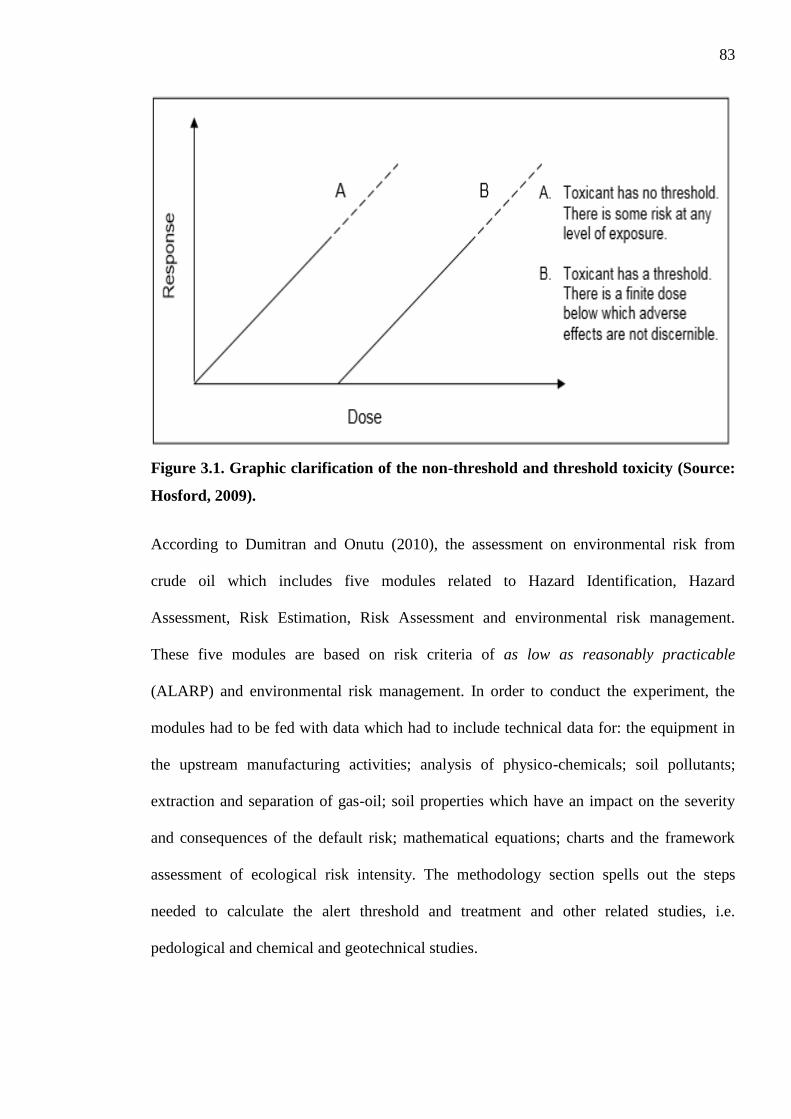
83
Figure 3.1. Graphic clarification of the non-threshold and threshold toxicity (Source:
Hosford, 2009).
According to Dumitran and Onutu (2010), the assessment on environmental risk from
crude oil which includes five modules related to Hazard Identification, Hazard
Assessment, Risk Estimation, Risk Assessment and environmental risk management.
These five modules are based on risk criteria of as low as reasonably practicable
(ALARP) and environmental risk management. In order to conduct the experiment, the
modules had to be fed with data which had to include technical data for: the equipment in
the upstream manufacturing activities; analysis of physico-chemicals; soil pollutants;
extraction and separation of gas-oil; soil properties which have an impact on the severity
and consequences of the default risk; mathematical equations; charts and the framework
assessment of ecological risk intensity. The methodology section spells out the steps
needed to calculate the alert threshold and treatment and other related studies, i.e.
pedological and chemical and geotechnical studies.

84
A study by Iturbe et al. (2004), based on the soil of a refinery located by the sea found that
the area was hydrocarbon contaminated and concentrations of up to 130000 mg/kg as
TPHs were detected. The study revealed that the hydrocarbon contamination was traced
back to the main contributors which were pipelines, valves, old storage tanks, additionally,
hydrocarbon contaminants were also caused by the land fill used for untreated hydrocarbon
sediments originating from the cleaning of storage tanks. The study evaluated the Health
Risk Assessment (HRA) by measuring the hazard indexes as well as the clean up level
values using the refinery soil.
Taken from the HRA compilation, the following actions were recommended: benzene
concentrations must be minimised in 8 of the 16 studied refinery regions to 0.0074-0.0078
mg/kg. Similarly, the concentration of vanadioum must be decreased in two regions up to a
concentration of 100 mg/kg. In the reduction of benzo(a) pyrene concentration from the
studied zones, only one zone needed to reduce to 0.1 mg kg(-1). The recommendations
were made in order to reduce the risks of the oil refinery substances on human health. The
overall results showed that the TPHs were reduced by around 52 %.
Sarmiento et al.‟s (2005) study showed that three principle approaches were utilised in
assessing potential human health risks from exposure to the hydrocarbon contamination of
TPH, i.e. the indicator approach, the surrogate approach and a mixed version. The
differences between these approaches were discussed in Sarmiento et al.‟s case study
research which was carried out in an area previously used as an industrial site affected by
petroleum products and planned for redevelopment as a recreational spot. They assessed
and took into account the TPH hazard elements towards human health using three ways of
possible exposure, i.e. inhalation of hydrocarbon vapour, digestion and dermal contact.
Initially, only indicator compounds were appraised. This was followed by classifying the
product as gasoline in the Quantitative Risk Assessment. Next an input parameter, a simple

85
hydrocarbon chains fractionation, was introduced. Lastly, the fractionation between the
aliphatic and aromatic terms of every group of hydrocarbons was measured. For each
specified pathway, the Site-Specific Target Levels (SSTLs) were computed. The
evaluation of results from various theories was carried out from the perspectives of both
the technical and economical. Scenarios whereby input concentration for a compound was
higher than the soil saturation boundary were also investigated.
A number of PAH are recognised mutagenic carcinogens; Irvine et al.‟s (2014)
investigation quantified the soil and atmospheric PAH concentrations in the Cold Lake
area to measure the excess lifetime cancer risk posed to the First Nations‟ populations of
the Alberta area, Canada. Both probabilistic and deterministic methods of risk assessment
were adopted and excess lifetime cancer risks were computed for exposures from
inhalation or unintentional consumption of soil. As indicated in the results, the mean
excess cancer risk for the First Nations‟ people involved in traditional rough country
activities in the area of Cold Lake through consumption was 0.02 new cases for every
100,000 with an upper 95 % risk level of 0.07 cases for every 100,000. Exposure to PAH
by means of breathing showed a maximum excess lifetime cancer risk of under 0.1 for
every 100,000 cases.
Crump‟s (1984) proposed benchmark dose (B.M.D.) was to estimate which doses could
produce an adverse change in the benchmark response (B.M.R.) taking into account the
background (see Hosford (2009)).“B.M.D methods were applied particularly to animal
data” (Hosford, 2009, p.8), however, the uncertain numerical factors (generic term) had to
be considered when extrapolating from the high doses in animal cases; these then had to be
divided by the „uncertainty factor‟ (fold factor) for human cases. Table (3.6) shows a
typical uncertainty factor as suggested in chemical risk assessment.
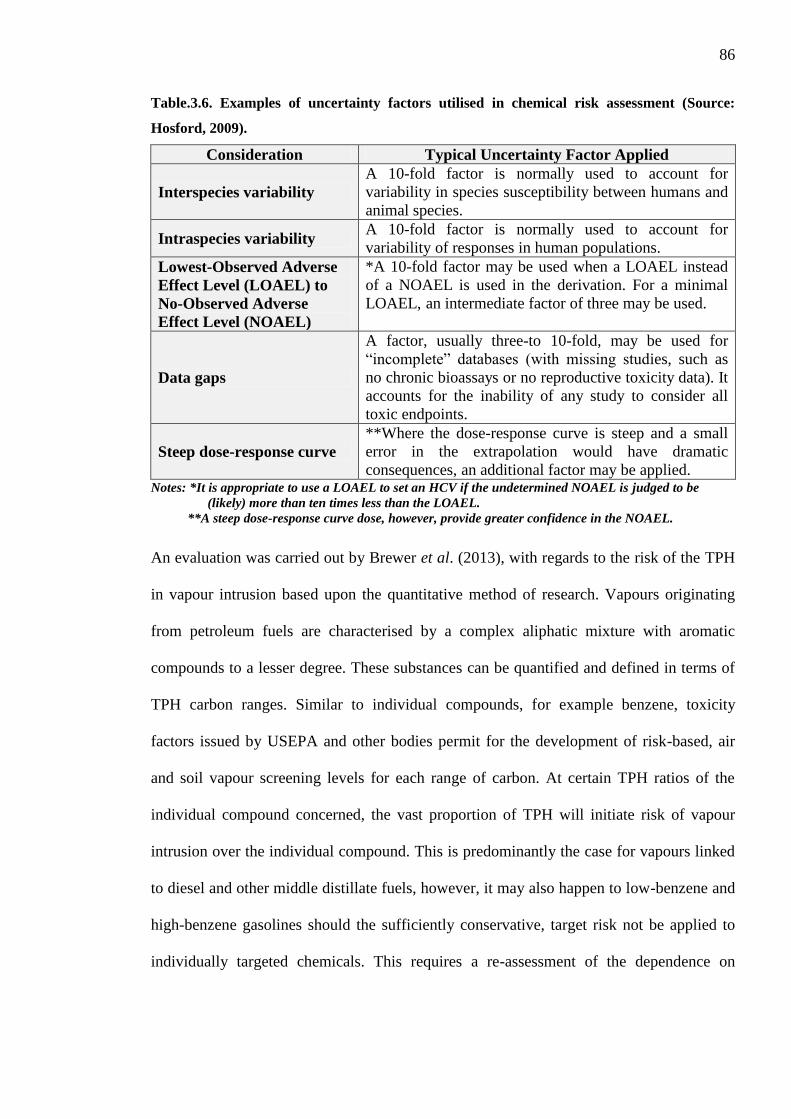
86
Table.3.6. Examples of uncertainty factors utilised in chemical risk assessment (Source:
Hosford, 2009).
Consideration Typical Uncertainty Factor Applied
Interspecies variability
A 10-fold factor is normally used to account for
variability in species susceptibility between humans and
animal species.
Intraspecies variability A 10-fold factor is normally used to account for
variability of responses in human populations.
Lowest-Observed Adverse
Effect Level (LOAEL) to
No-Observed Adverse
Effect Level (NOAEL)
*A 10-fold factor may be used when a LOAEL instead
of a NOAEL is used in the derivation. For a minimal
LOAEL, an intermediate factor of three may be used.
Data gaps
A factor, usually three-to 10-fold, may be used for
“incomplete” databases (with missing studies, such as
no chronic bioassays or no reproductive toxicity data). It
accounts for the inability of any study to consider all
toxic endpoints.
Steep dose-response curve
**Where the dose-response curve is steep and a small
error in the extrapolation would have dramatic
consequences, an additional factor may be applied. Notes: *It is appropriate to use a LOAEL to set an HCV if the undetermined NOAEL is judged to be
(likely) more than ten times less than the LOAEL.
**A steep dose-response curve dose, however, provide greater confidence in the NOAEL.
An evaluation was carried out by Brewer et al. (2013), with regards to the risk of the TPH
in vapour intrusion based upon the quantitative method of research. Vapours originating
from petroleum fuels are characterised by a complex aliphatic mixture with aromatic
compounds to a lesser degree. These substances can be quantified and defined in terms of
TPH carbon ranges. Similar to individual compounds, for example benzene, toxicity
factors issued by USEPA and other bodies permit for the development of risk-based, air
and soil vapour screening levels for each range of carbon. At certain TPH ratios of the
individual compound concerned, the vast proportion of TPH will initiate risk of vapour
intrusion over the individual compound. This is predominantly the case for vapours linked
to diesel and other middle distillate fuels, however, it may also happen to low-benzene and
high-benzene gasolines should the sufficiently conservative, target risk not be applied to
individually targeted chemicals. This requires a re-assessment of the dependence on
87
benzene and other individual compounds as a separate tool in the evaluation of vapour
intrusion risk associated with petroleum.
Nathanail et al. (2007), claim that in assessing the risk derived from the polluted areas, risk
assessment is formed and grouped into two phases and two sub-phases namely Phase 1a-
Hazard Identification, Phase 1b- Hazard Assessment, Phase 2a -Risk Estimation and Phase
2b- Risk Evaluation.
Bowers and Smith (2014) carried out an assessment on the risk to human health caused by
vehicle petroleum fuels within the soil. A suitable set of Constituents of Petroleum
Concern (COPCs) ought to be evaluated and managed in order to provide vigorous
management of potential risks and to minimise redundant chemical analyses and
evaluation of constituents that hardly (or never) cause any risk to human health. A
procedure in identifying COPCs for petroleum fuel releases has been proposed based on
widely accepted practices for human health risk assessment and available data related to
fuel composition and the toxicity of chemicals. Lists of COPC are used to assist in
investigating and assessing the risks at sites where petrol, diesel, and kerosene/jet fuels are
believed to have been released. Broadly, these lists are relevant and may reinforce site-
specific assessment of environmental settings and related risks.
3.5.2 Human Health Risk Assessment (HHRA) Models
As mentioned by Searl (2012), besides CLEA, SNIFFER and LQM models, there are some
computer software packages which are accessible commercially in the UK which support
detailed quantitative risk assessment (DQRA) for human health risks. These packages were
designed mainly to assist in the assessment of contaminated risk in the U.S. (RBCA and
RISC-5 models). The software packages for the U.S. market involve more sophisticated
techniques to model behaviour of contaminants in air and water in comparison with the

88
method used by CLEA. As such, the comparative influence of these pathways to overall
exposure by the contaminant will vary accordingly.
Tables 3.7 and 3.8 were prepared (by the author) to allow for comparisons between CLEA,
SNIFFER, RBCA and RISC 5 model packages, so as to choose the most relevant package
(model) acknowledging local conditions in Kuwait (Nathanail et al., 2002; Jeffries and
Martin, 2009; Searl, 2012; RISC-5, 2011).

89
Table 3.7. Comparison between different model applications in the risk assessment.
Model
Name
Exposure Pathway Assessment Models
Risk
Assessm
en
t
Refer
ence
s Air Ground Water
Sh
ow
er
Sh
ow
er S
urfa
ce
Irrig
atio
n W
ater
Soil
Inh
ala
tion
ind
oo
r
Inh
ala
tion
ou
tdo
or
Ing
estion
Der
ma
l
Inh
ala
tion
Veg
etab
le
Up
tak
e
Ing
estion
Der
ma
l
Inh
ala
tion
of
Pa
rticula
tes
Veg
etab
le
Up
tak
e
CLEA-
2002 × × × × × × ×
In Human
Health
(Nathanail et al., 2002, p.49 and
Jeffries and Martin, 2009)
SNIFFER × × × × × × × In Human
Health
(Nathanail et al., 2002, p.37)
RBCA × × × In human
health and
ecosystem
(Nathanail et al., 2002, p.39 and
Searl, 2012, p.29)
RISC-5 In human
health and
ecosystem
(Searl, 2012, p.29 & 30 and
RISC-5, 2011 )
Notes: Considered in model application, × Not considered in model application.

90
Table 3.8. Limitations and suitability of various models in relation to Kuwait conditions.
Model
Name Limitation
Appropriation for
Kuwait Climate
CLEA
Does not consider the domestic use of on-site
groundwater (ingestion of groundwater,
dermal contact of showering) (Nathanail et
al., 2002, p.49) Very specific model for
UK. As such, it takes
consideration of UK
climate. SNIFFER
Exposure via the consumption of drinking
water or by inhalation of vapour through the
use of water (swimming) is not included
(Nathanail et al., 2002, p.37).
RBCA
Exposure from vegetable uptake via
groundwater; and exposure via showering
and irrigation water are not taken into
consideration (Searl, 2012, p.29).
Specific model for U.S.
where the climate in
Kuwait nearer than that in
UK. Furthermore, it is old
model compared with
RISC-5.
RISC-5
Take into consideration all the above models
limitations (Searl, 2012, p.29 &30 and RISC-
5, 2011).
Specific model for U.S.
nearer to Kuwait climate.
Various studies which relate to the risk assessment evaluation of soil contaminated with oil
residue as well as their influence on human health were reviewed. It was discovered in a
number of studies that the Risk Based Corrective Action (RBCA) toolkit is able to
integrate the risk assessment procedures, e.g. Hazard Identification, Exposure Pathways
Assessment, Toxicity Assessment and Risk Characterisation.
As stated in the GSI Environmental (n.d.), Risk-Based Corrective Action (RBCA), is
regarded as a practical management procedure with clear emphasis on safeguarding human
health and the environment and at the same time encouraging energy and cost-efficient
remedies to allow limited resources to be aimed at the most hazardous areas. The basis of
the RBCA framework is the establishment of a criteria for site-specific environmental
clean-up resulting from a tiered risk evaluation methodology. In other words, the RBCA
Tool Kit for Chemical Releases is a complete modelling and software for characterising
risks. It is intended to conform to the ASTM Standard Guide for Risk-Based Corrective
91
Action (E-2081) requirements for Tier 1 and Tier 2 RBCA evaluations for chemical release
sites alongside the traditional calculations for risk assessment.
The contaminant transport models and risk assessment tools are incorporated into the
software to compute baseline risk levels and develop standards for risk-based clean-ups for
a wide range of soil, groundwater, surface water, and air exposure pathways. The features
which are user friendly coupled with reorganised graphical interface features of this
software are the key elements for making a main instrument to manage RBCA and generic
risk assessment calculations for both straight forward and complex problems (GSI
Environmental, n.d.).
A study was undertaken by Pinedo et al. (2012) comprising a site specific risk assessment
for the distribution and concentration of TPH fractions using the RBCA framework. This
study was conducted in the Spanish, densely inhabited, average sized city of Santander
with approximately 182,000 inhabitants; it was also used as a case study. In this study, two
hydrocarbon contamination routes were considered, namely Volatilization and Particulates
to Outdoor Air Inhalation (through ambient air volatilization of hydrocarbon contaminants
from affected soils and small particles of superficially affected soil) and Surface Soil
(through direct ingestion, dermal contact and inhalation). From the results, it appears that
the Outdoor Air pathway registered lower risk as shown from the HQ values which are less
than the upper limit of 1.0. Individual fraction soil risks are also lower than the HQ limit;
however the cumulative risk is nearly 1.6 times above this threshold. This high cumulative
risk was primarily the result of the aromatic EC16- EC21 fraction, which constituted nearly
half of the total risk. It was found only in the total TPH of the superficial soil, registering a
value of 1.6 times above the Site-Specific Target Levels (SSTLs).
Similarly, Asharaf (2011) studied the method employed by the Bahrain Petroleum
Company (Bapco) to: identify the sites contaminated with hydrocarbon; assess the

92
potential risk to human health and the environment; and to suggest any necessary
preventive measures by adopting the fundamentals of Risk Based Corrective Action
(RBCA).
Together with a desk based study, a phased strategy was used followed by a
comprehensive assessment consisting of the boring of 40 window sample locations for soil
and installing a total of 28 groundwater monitoring boreholes. More than 200 soil and
groundwater samples were taken and analysed for hydrocarbons and heavy metals. This
was followed by developing a conceptual site model in accordance with the Site-Pathway-
Receptor linkage. The outcomes of the soil and groundwater analysis were used in
deciding the likely risk to human health and the environment.
Chen et al. (2004) applied a method related to health risk assessment in deriving the levels
of clean-up at a site contaminated with a fuel oil spill. The application was described in
four different risk assessment techniques in an effort to undertake a risk assessment
exercise and demonstrate the application method at the site of the fuel oil spill. These
techniques included the North Carolina risk analysis framework, the Illinois tiered
approach to correction objectives, the RBCA software for chemical releases, and Exposure
and Risk Assessment Decision Support System. On completion of the risk evaluation
procedures, a determination of the groundwater and soil treatment aimed at object
compounds, (namely TPH), xylenes, toluene, ethylbenzene and benzene) was performed.
The computed remediation levels satisfy the minimum requirement for target risk
benchmarks, i.e. a cancer risk of 1×10⁻⁶
and risk proportion of one. From the results of this
research, RBCA appears to be a more comprehensive and conservative base for closure of
site.
Tomasko et al. (2001), presented an engineering method which could be utilised in
predicting maximum NAPL concentrations in the groundwater caused by NAPL spills. The

93
risks associated with NAPL within the site were evaluated by means of the U.S.
Environmental Protection Agency's tiered risk-based corrective action (RBCA) system.
Conservative assumptions were utilised in Tier 1 with minimal site-specific information
whilst more detailed site-specific information was needed under Tier 2. This method of
screening was formulated by deriving a systematic solution for a partial differential
equation defining the movement of NAPL through the unsaturated sector.
3.5.3 Risk Integrated Software for Soil Clean-up (RISC) for HHRA
An appraisal was carried out on previous studies concerning the evaluation of risk
assessment of oil residue contaminated soil as well as on their effect on human health by
means of the RBCA toolkit. A number of studies noted RISC-5, software that can be used
with other risk assessment methods including the Exposure Pathways Assessment, the
Toxicity Assessment and Risk Characterisation.; Hazard Identification was, however, not
included in the assessment. It was also discovered that RISC-5 and RBCA software were
similar; but the former was found to be more useful, flexible and easier to use.
The main differences between RISC software and RBCA are that the former offers highly
intuitive graphical interface, allows for pathways, compound and receptor additivity;
additionally, the results of transport models can be utilised in the presence of a phase-
separated product; the vadose zone model is present and transient groundwater models,
probabilistic. (Monte Carlo) exposure capabilities are also available in the software (RISC-
5) and includes a critical pathway - indoor showering which is not provided in the RBCA
Toolkit. It also includes a number of other models which are not available in the RBCA
model in ASTM E1739 but are required for some typical risk cases. Other models are:
Johnson and Ettinger (1991) indoor air model; Domenico (1987) model for groundwater;
and Green-Ampt (1911) model for considering biodegradation of dissolved chemicals in
the vadose zone (Spence and Walden, (2001)).

94
RICS-5 software can be employed in the assessment of severe effects to human health
(carcinogen and non-carcinogen) based on fourteen exposure pathways at contaminated
sites. Further, RICS-5 offers distinctive features and is able to perform a reverse
computation on risk. This entails performing calculations on the extent of a clean-up for a
given risk value including the conventional forward risk calculation. According to Spence
and Walden (2001), RICS-5 offers fate and transport models in assessing concentration of
receptors in groundwater as well as indoor and outdoor air.
Armah et al.‟s (2012), study assessed the risks of water sediment and biota and their
adverse impact on human health by means of RISC-4.02 in the Tarkwa Gold mining area.
The research was formulated to evaluate the risks to human health through Central
Tendency Exposure (CTE) and Reasonable Maximum Exposure (RME) scenarios to
residents. The residents were comprised of grown-ups and youngsters from arsenic,
manganese and lead exposures on the ground surface and in groundwater. The outcome
revealed that HQ for these contaminants are mainly within the tolerable risk range outlined
by the United States Environment Protection Agency (USEPA). The RME of Mn from oral
contact for Youngsters (HQ of 18) is noticeably greater than the USEPA acceptable risk
figure of 1.0.
At some sites, the RME of Mn through oral contact for adults also surpassed the standard,
however, a comparison of contributions of dermal and oral contact to the health risk,
revealed that the former accounted for more. Carcinogenic risks to resident grown-ups
caused by the exposure to arsenic demonstrated RME values which varied from 5.0 x 10⁻⁴
to 1.1 x 10⁻³
. They constitute up to 11 folds higher than the USEPA acceptable range for
excess risk of cancer. Arsenic-linked cancer risks to resident grown-ups for CTE varied
from 3.7 x 10⁻⁴
to 6.7 x 10⁻⁴
; these are higher than the acceptable range (based on USEPA)
for excess risk of cancer. Similarly, the risks of cancer to resident youngsters for CTE and
95
RME cases were higher than the USEPA acceptable range for excess cancer risk. These
figures were more than 210 times higher than the USEPA acceptable range for excess risk
of cancer.
3.5.4 Oil Contamination Risks on Human Health
Various studies were carried out and appraised with respect to evaluating the risk
assessment of soil contaminated with oil residue as well as their severe effects on human
health. A number of studies focussed on the human diseases caused by the exposure to
contamination whether the term of illness was short or long. As stated by Amat-Bronnert et
al. (2007), Campbell et al. (1993), Ordinioha and Brisibe (2013) and Osman (1997), the
influence of hydrocarbon contamination on human health can occur at various stages of
illness, including - physical, mental, genetic, heart, headaches, throat irritation and itchy
eyes, infertility, cancer, lumbar pain, migraine and dermatitis.
A cross-sectional study was conducted by Campbell et al. (1993) whereby a number of
people exposed to the MV Braer oil spill (N = 420) were matched against a control group
(N = 92) in Hillswich, about 95 km to the north of the site. As revealed from the result,
immediately after the incident, the population suffered from headaches, throat irritation
and itchy eyes for a period of two days. As for the long term effects, 7 % of the population
exposed to the contamination felt that the oil spill had had a huge influence on their health.
According to Ordinioha and Brisibe (2013), published data on crude oil spills in the Niger
Delta Region, Nigeria, and animal studies confirmed that direct contact with the crude oil
of Nigeria could be hemotoxic and hepatotoxic and could result in infertility and cancer.
Osman (1997) examined the adverse health effects resulting from the Kuwaiti oil lakes
residue in 1991. Based on his study, a survey performed in Kuwait healthcare centres
demonstrated a rise in respiratory complaints directly proportional to the rise in air
particulates recorded during the same period after 1991. Within that period, the number of
96
people looking for treatment for psychiatric illness, bronchiecteasis, chronic bronchitis and
emphysema, gastrointestinal illness and heart disease showed a sharp rise.
3.6 Summary
Considering that Kuwait is considered one of the countries in the world which has been
most seriously contaminated since 1990 (Gay et al., 2010), the main contribution of this
study is to develop a ground model for the oil lake contaminated soil of Kuwait (caused by
the Iraqi invasion in 1990) using RISC-5 model. This contamination might not only affect
the physical properties of soil but is also likely to threaten the ecology and human health
through chemical risks. This study investigates the geotechnical and geochemical
properties and classifies the pollutants existing in the hydrocarbon contaminated soils, also
the carcinogenics and non-carcinogenics.
The study will also investigate the influence of oil lakes residue on the Human Health Risk
Assessments and determine the potential levels of risk posed to any future urban
developments within the affected areas. More specifically, this will be achieved by using
the risk assessment of the RISC-5 software to evaluate chemically any signs of
carcinogenic elements found in the hydrocarbon contaminated soils that may influence the
health of human, animal and plant life, even if the geotechnical properties of the
hydrocarbon contaminated soils are physically ready for construction.
To the best of author knowledge, no studies have investigated the geotechnical and/or
geochemical characterisation of the actual hydrocarbon contamination of the soil in the
Greater Burgan Field of Kuwait since 1990; so far all studies have been based on
replicating the effect of contamination by mixing the soil with artificial crude
contamination in the laboratory. Al-Sanad and Ismael (1997) admitted that researchers
could not extract actual samples from the base of the dry Burgan oil lakes because there is
no access to these lakes for security reasons, i.e. the existence of mines and oil-sand sludge
97
which covered the ground in nearby areas. It is worth mentioning that this study is
considered a pioneer study since it has collected the actual hydrocarbon contaminated soil
samples from the dry oil lakes found in the Kuwaiti Burgan Oil Field. All required
permissions and safety precautions insisted on by the Kuwait Oil Company (KOC) and the
University of Portsmouth (UoP) were signed and followed by the researcher who takes full
responsibility regarding any risk that might he might face during the sample collections.
(Figures from A.4.5a to A.4.6f in Appendix-D)
The following significant reasons encouraged the researcher to select the Greater Burgan
Oil Field (Al-Magwa area) as the main site for this study:
(1) No study has investigated the geotechnical and geochemical
characterisations of the actual dry oil lake contaminated soil in the
Greater Burgan Oil Field (Al-Magwa area) for 25 years.
(2) The Greater Burgan Field (among other sites) contains the largest
hydrocarbon polluted area (25.6 Km2) and Volume (14,520,000 m
3) in
Kuwait. (Table (2.2) Chapter two, page (38)).
(3) The largest hydrocarbon contamination occurred in Kuwait in the
Burgan Oil Field since it constitutes 40 % of the overall contaminated
volume (Al-Duwaisan and Al-Naseem, 2011).
(4) It is located near to the city and urban areas and the surrounding areas
of the Burgan Oil Field will be undergoing some engineering
construction in the next five years.
(5) A high percentage of Kuwaiti citizens have contracted fatal diseases,
including asthma and lung cancer, since 1990 due to carcinogenic
substances, i.e. hydrocarbon chemical compositions found in oil
contaminated soil which can greatly influence human health.

98
4. GREATER BURGAN OIL FIELD INVESTIGATION
4.1 Introduction
The objectives of this research will be attained through the implementation of an
experimental methodology which will include collection of samples followed by
geotechnical and geochemical tests in the laboratory. This chapter will describe and outline
the experimental programme, including Phase I concerning preliminary selected sites for
the study (both contaminated and non-contaminated), initial soil sample collection, final
selected sites (both contaminated and non-contaminated) and Phase II which will request
the soil sample collection at two different final selected sites.
The methods and procedures followed in conducting the necessary tests on the soil samples
collected from contaminated (dry oil lake) and non-contaminated sites are described in
terms of their geotechnical, geochemical and hydrocarbon characteristics. Statistical
analysis has been undertaken to further integrate the data and to support the results.
Section 4.2 describes the phases and the experimental scope of the study. The selection
process of the initial site is described in Section 4.3. Details of the location finally selected,
i.e. the Greater Burgan Oil Field-Al Magwa area and the main soil sampling approach
followed are described in sections 4.4 and 4.5, respectively. Section 4.6 clarifies the
sampling method at contaminated and non-contaminated sites. Section 4.7 outlines the soil
characterisation and the methodology. Section 4.8 explores and classifies the data from the
laboratory via statistics method.

99
4.2 Investigation Design
The experimental phases set out in this chapter are aimed at achieving the goal of the study
as described in Section 1.1. A comprehensive experimental research programme was then
designed (Figure 4.1). The programme was split into six phases as follows:
Phase I
Preliminary site selection - carried out by identifying the hydrocarbon contaminated sites
in Kuwait. The closest site to the most densely populated area of Kuwait together with the
amount of hydrocarbon contamination encountered was chosen in order to select sites for
preliminary soil sampling and to verify that the hydrocarbon contamination was still
present after 25 years.
Phase II
Confirmation of the final site location, i.e. dry oil lake; identification of field hazards &
restrictions; requirements for Health and Safety; walkover survey and description of the
site.
Phase III
Collection of major soil samples at the chosen site of the Greater Burgan Oil Field (Al-
Magwa region) involving the detailed collection of soil samples at both a dry oil lake site
(hydrocarbon contamination) and a non-contaminated site for control purposes.
Phase IV
Investigation of the geotechnical characteristics of the soil samples at both the dry oil lake
and the non-contaminated sites. These include the Atterberg Limits; PSD; SEM;
permeability (Hydraulic Conductivity); and Direct Shear strength parameters. A
geochemical investigation was undertaken on both the contaminated (dry oil lake) and the
non-contaminated sites by means of characterising the soil samples chemical properties
including - the pH value; water soluble Cl- and (SO3 & SO4); EA and GC-MS tests.
100
Phase V
Carrying out an assessment of the risk on human health due to hydrocarbon contaminated
soil from the dry oil lake site – (detected soil samples with hydrocarbon). This will be done
by means of applying human health risk assessment scenarios, e.g. Hazard Identification;
Hazard Assessment; Risk Estimation and Risk Evaluation.
Phase VI
Utilising RISC-5 software (RISC-5, 2011) on hydrocarbon contaminated soil from the dry
oil lake, i.e. soil samples with hydrocarbon, to determine concentration of hydrocarbons
which may cause adverse impacts on human health as categorised in terms of carcinogenic
and non-carcinogenic elements. Developing ground models by assessing the probable
magnitude of risk and calculating soil clean-up values where appropriate in the site to be
selected for any prospective urban developments.
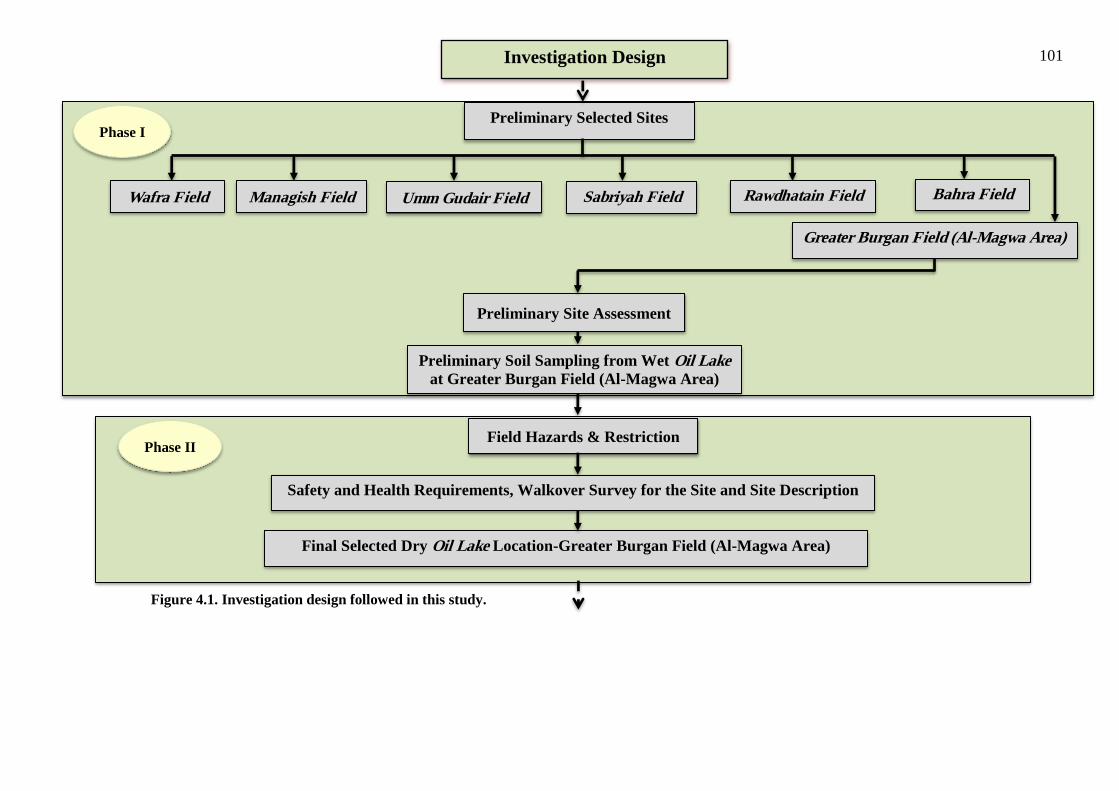
101
Figure 4.1. Investigation design followed in this study.
Investigation Design
Phase I Preliminary Selected Sites
Preliminary Site Assessment
Phase II Field Hazards & Restriction
Safety and Health Requirements, Walkover Survey for the Site and Site Description
Final Selected Dry Oil Lake Location-Greater Burgan Field (Al-Magwa Area)
Wafra Field Managish Field Umm Gudair Field Sabriyah Field
Rawdhatain Field
Bahra Field
Greater Burgan Field (Al-Magwa Area)
Preliminary Soil Sampling from Wet Oil Lake
at Greater Burgan Field (Al-Magwa Area)
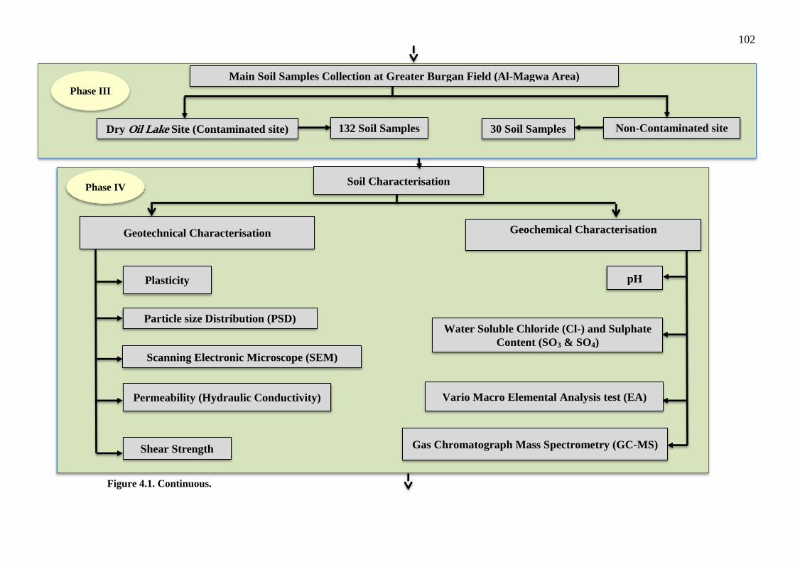
102
Figure 4.1. Continuous.
Phase III
Phase IV Soil Characterisation
Geotechnical Characterisation Geochemical Characterisation
Plasticity
Shear Strength
Particle size Distribution (PSD)
Scanning Electronic Microscope (SEM)
Permeability (Hydraulic Conductivity)
pH
Water Soluble Chloride (Cl-) and Sulphate
Content (SO3 & SO4)
Vario Macro Elemental Analysis test (EA)
Gas Chromatograph Mass Spectrometry (GC-MS)
Main Soil Samples Collection at Greater Burgan Field (Al-Magwa Area)
Dry Oil Lake Site (Contaminated site) Non-Contaminated site 30 Soil Samples 132 Soil Samples
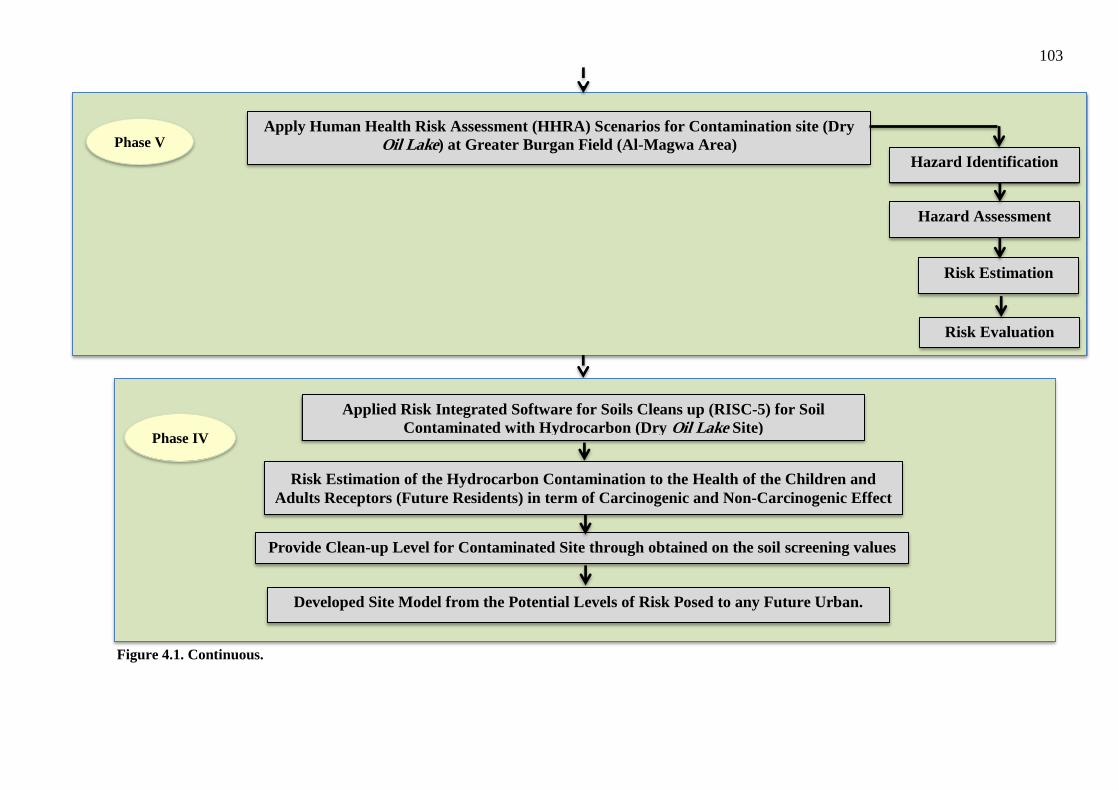
103
x
ssdddddddddddd
dddd
Figure 4.1. Continuous.
Phase V Apply Human Health Risk Assessment (HHRA) Scenarios for Contamination site (Dry
Oil Lake) at Greater Burgan Field (Al-Magwa Area)
Hazard Identification
Hazard Assessment
Risk Estimation
Risk Evaluation
Applied Risk Integrated Software for Soils Cleans up (RISC-5) for Soil
Contaminated with Hydrocarbon (Dry Oil Lake Site)
Risk Estimation of the Hydrocarbon Contamination to the Health of the Children and
Adults Receptors (Future Residents) in term of Carcinogenic and Non-Carcinogenic Effect
Provide Clean-up Level for Contaminated Site through obtained on the soil screening values
Developed Site Model from the Potential Levels of Risk Posed to any Future Urban.
Phase IV
104
4.3 Preliminary Site Selection
Cho et al. (1997) and PEC (1999) have stated that hydrocarbon soil contamination and the
remnant oil lakes are situated in the seven main oil-producing fields of Kuwait, namely:
Rawdhatain; Sabriyah, Umm Gudair; Managish; Wafra, Bahra; Greater Burgan Field
(Ahmadi, Magwa; and Burgan Sectors) (as illustrated above, Figure 2.15 and Table 2.3).
Therefore, the chosen sampling area was situated adjacent to the main oil producing areas
of Kuwait, i.e. the Greater Burgan Field (Ahmadi, Al-Magwa and Burgan Sectors) in the
south of Kuwait. This site was selected for the following reasons:
The worst hydrocarbon contamination incident took place in the Burgan
Field which accounts for 40 % of the entire hydrocarbon contaminated
volume in Kuwait (Al-Duwaisan and Al-Naseem, 2011, p.440).
The Greater Burgan site contains the largest oil lake area in Kuwait
originating from the Iraq invasion. According to PEC (1999), the
coverage of soil contaminated with oil lakes residue in the Greater
Burgan field covered an area of 25.6 km2 with a 14,520,000 m
3 volume
of soil.
Its location is near both the city and the urban areas of Al-Ahmadi,
Jaber Al-Ali, Sabah Al-Salam and Jeleeb Al-Shuyoukh. All of these
areas are heavily populated (Figure 4.2). The adjacent areas are,
therefore, likely to be developed in the future as urban expansion
demands grow thus requiring construction work.
It is predicted that these areas will be in high demand for prospective
development projects; the Kuwaiti Government intends to start a mega
project in 2013 which will last until 2020 (UK Foreign and
Commonwealth Office, 2014; Almarshad, 2014, p.49).

105
Figure 4.2. Distance of the Greater Burgan Oil Field and the main residential areas (Source: GM, n.d.).
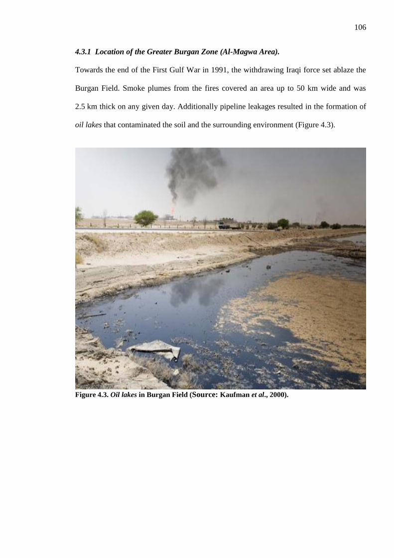
106
4.3.1 Location of the Greater Burgan Zone (Al-Magwa Area).
Towards the end of the First Gulf War in 1991, the withdrawing Iraqi force set ablaze the
Burgan Field. Smoke plumes from the fires covered an area up to 50 km wide and was
2.5 km thick on any given day. Additionally pipeline leakages resulted in the formation of
oil lakes that contaminated the soil and the surrounding environment (Figure 4.3).
Figure 4.3. Oil lakes in Burgan Field (Source: Kaufman et al., 2000).

107
The Greater Burgan Oil Field is situated within the Arabian Basin in Kuwait. It is the
world‟s largest clastic oil field which covers an area of approximately 320 square miles
(828 km2) in the south-east of Kuwait. The field is split into the Al-Magwa, Al-Ahmadi
and Burgan areas based upon the presence of three structural domes as shown in Figure
4.4. The border along the northern Al-Ahmadi/ Al-Magwa and the Burgan sectors is the
complex of the Central Graben Fault. The Burgan Field, being the largest sandstone oil
field in the world, is situated 35 km south of Kuwait‟s capital City close to Ahmadi.
Figure 4.4. The Greater Burgan sectors (Burgan, Al-Magwa & Al-Ahmadi Fields) in Kuwait
(Source: Kaufman et al., 2000).
Sites Location

108
4.3.2 Preliminary Assessment
A preliminary investigation was undertaken to determine the most suitable initial sampling
locations and the sample sizes, this was carried out by reviewing and analysing the
gathered data. The received information had been collected from websites and also from
requests to relevant personnel from private contractors for the Greater Burgan Oil Field
and the Kuwait Oil Company (KOC). Information from the test areas provided by these
firms was investigated and examinations were carried out on the test area. It was essential
that the preliminary sampling locations were determined based upon the consistency of the
soil conditions to find out whether they could provide accurate representation of the test
area. In order to assess the location of sampling points and sample sizes, a large quantity of
data was required to be collected.
4.3.3 Preliminary Soil Sampling
A total of 5 soil samples were taken from two separate sites within the Greater Burgan
Field (Al-Magwa area) consisting of 2 kg each of contaminated and non-contaminated
samples. One disturbed hydrocarbon contaminated soil sample was extracted manually
from a wet oil lake at a depth of 0.5 m using a shovel. For the non-contaminated samples, a
total of 4 undisturbed control soil samples were taken from various depths, i.e. 0.5 m, 1.0
m, 2.0 m and 4.0 m below ground within the same area using borehole equipment (Plate
A.4.1).
Samples collected from the wet oil lake (contaminated) and non-contaminated sites were
delivered to the University of Portsmouth laboratory for classification and testing. A
preliminary testing procedure was carried out on these soil samples to ascertain the TPH
concentration level. Preliminary characterisation tests, includes GC-MS, was performed on
the soil samples to examine the total TPH concentration.

109
The average TPH concentration was 9.81 mg/kg. for the 4 soil samples extracted from the
designated non-contaminated site of the Greater Burgan Field (Al-Magwa area), In
comparison, the TPH concentration for disturbed soil samples taken at the designated
contaminated site within the same area was 18683.37 mg/kg (Tables A.4.1 & A.4.2 and
Figures A.4.1 & A.4.2).
4.4 Final Selected Location (Greater Burgan Field - Al-Magwa Area)
Based on the results from the preliminary soil sampling, it was confirmed that the Greater
Burgan Field (Al-Magwa area) has remained contaminated since the 1st Gulf War (1990).
During the soil investigation process, a number of obstacles were encountered-especially in
the early part of the work- allowing entry into the Greater Burgan Field, this had affected
the soil sample schedule, these obstacles were:
These oil lakes are categorised as being within the authority of the
Kuwait Oil Company (KOC) and the Kuwaiti Defense Ministry. As
such, entry to the project site is limited to employees of the private
contracting companies. The non-contaminated site has no entry
conditions for the collection of soil samples.
Gaining admission to the KOC‟s officer-in-charge of the issuance of
official permits to enter the site legally to take samples was a lengthy
process.
In view of the large organisational structure of the KOC - which is divided
into several sectors - it took a very long time to assess, search for and
collect the required information from relevant departments. The problems
included complying with their Quality System requirements to identify the
correct department-in-charge and present them with all project
documentation plans; main samples plan; and the official letter from the
110
University of Portsmouth. The Greater Burgan Oil Field comes under
more than two sectors.
The area where the oil lakes are located is extremely dangerous as it
contains mines and unexploded ordnance left behind after the war.
Collecting samples during the summer season (hot and arid climate) at
these hazardous sites is not permitted. This is because during the hot and
arid climate, the hydrocarbon contamination evaporates into the air.
Towards the end of the finalised location, an entry permit was issued so that the work plan for
sampling and methodology could be submitted to the relevant department of the KOC.
4.4.1 Site Hazards and Restrictions
A number of meetings and visits were scheduled with the relevant managers from various
departments in the KOC responsible for the oil lake sites at the Greater Burgan Field.
These included the: Health Safety and Environment Department (HS & E); Production
Operation Department (PO); and Research and Technology Department (R & T).
Furthermore, on 17th
July, 2012. A confidentiality agreement was executed at KOC‟s main
office in the Al-Ahmadi area outside the Greater Burgan Field security fence, between
their Research and Technology Department (R & T) and the University of Portsmouth
(UoP).
The UoP was represented by the PhD Research student on behalf of his supervisors. Upon
signing of the agreement, on 22nd
August, 2012, an Explosive Ordnance Disposal (EOD)
clearance was requested from the HS&E Department by the T&C department for entry into
the main samples‟ site (Figures A.4.3a, A.4.3b, A.4.3c, A.4.4a, A.4.4b, A.4.4c, A.4.4d,
A.4.4e and A.4.4f).
The area of the Greater Burgan Field is regarded as the major economic region for
generating revenues for the State of Kuwait; it is vibrant with numerous engineering

111
projects, therefore, a lengthy procedure was required to schedule meetings with the HS&E
and PO departments to finalize the entry permit for the site. Furthermore, collection of
samples at the hydrocarbon contaminated field area was not permitted during the summer
season due to the increase in hydrocarbon evaporation - potentially highly dangerous – this
was one of the major obstacles to the project.
Finally, on 11th
November, 2012, a temporary entry permit was obtained allowing for a
meeting with the experts from the HS&E and PO departments: Meeting one was to finalize
and select the specific site location (dry oil lake) and present the main sampling plan. The
second and final meeting was conducted on 18th
November, 2012 with the same personnel
to discuss and present the final sampling plan and to determine the number of skilled
labourers required for the collection of samples (Figures A.4.5, A.4.6 and A.4.7).
All meetings with regards to the main sampling plan and time schedule were finalised in
accordance with the conditions and requirements, as follows:
Reducing sample collection quantity from 400 to only 132 samples.
Disagreement as to extraction of the hydrocarbon contaminated soil
samples using borehole truck method so as to obtain undisturbed soil
samples for Direct Shear test; agreement was only with the trial pit
method. This was because of health and safety issues, e.g. the ground
condition of the dry oil site was very dense, unstable and dangerous which
could pose serious risks to KOC labourers. As such enquiries were raised
with KOC technical staff, i.e. project supervisors and the INCO Lab firm
in Kuwait in order to collect undisturbed samples without a borehole
truck. They suggested that the only means of collecting the samples would
be to fabricate tubes with fixed lengths and diameters so that the
undisturbed soil samples could be extracted (Figure A.4.8).

112
The time for sample collection was limited from 7.00 a.m. to 11.00 a.m. as
the dry oil lake area can be very hazardous to the labourers health due to
the increasing of hydrocarbon evaporation in the afternoon period. As such
the working hours were based on this constraint.
The sample collection should be halted in the case of rain because the wet
conditions of the site would be dangerous for the workers.
The existing KOC site conditions were studied by means of site visits, reviewing
reports from private construction firms operating within the Greater Burgan Oil
Field (Al-Magwa area) as well as requesting any relevant information regarding the
site. In fact, Al-Duwaisan and Al-Naseem (2011, p. 441) stated that the highest
hydrocarbon content of the contamination area was encountered at a depth range of
0.15 m to 1.2 m; the soil sampling plan at the contaminated site became clearer
with this information. The dimensions of the sample area were 100 m x 100 m. A
total of 25 Trial Pits (T.Ps) were excavated to obtain more contaminated soil
samples. The depths of the trial pits varied from 0.0 m, 0.25 m, 0.5 m, 1.0 m and
2.0 m (section 4.5 for further details).
4.4.2 Site Safety Requirements
Due to the nature of the site precautionary measures the following had to be
complied with at all times:
No food or drink should be consumed at site during the collection of
samples.
No smoking allowed within the site as the area is flammable due to the
presence of hydrocarbon in the ground.

113
Workers are to be reminded to ensure hands are washed before drinking,
eating or even smoking due to possible hydrocarbon contamination.
A risk assessment form from the University of Portsmouth (UoP) was
prepared and approved prior to data collection so as to ensure that the
researcher was fully aware of the risks expected at the sample collection
area (Figures A.4.9a, A.4.9b, A.4.9c & A.4.9d).
4.4.3 Site Walkover Survey
A walkover survey was undertaken at the site so as to identify, analyse, and
characterise the dry oil lake sites and also to note any changes in texture and colour
of the potentially contaminated soil. The survey was also carried out to: physically
view the type of contaminant of the dry oil lake; appreciate the general conditions
of the field; make the sampling team familiar with site characteristics; and explore
the site by identifying the locations of oil hotpots prior to the selection of sampling
Trial Pits (T.Ps) locations and sample extraction methods.
A number of construction firms with ongoing construction works within the test area were
approached and details concerning the ground conditions, boreholes, trial pits and
variations in groundwater were requested and collected.
The site walkover survey provided an organised, on-site field map indicating the sampling
locations. Additionally, data obtained from these construction firms operating within the
same area was collated, reviewed and incorporated into the map. Towards the end of the
walkover survey, a final map of the sampling zone, showing possible sampling points, was
prepared. The workforce and equipment required to perform the sampling work was also
identified.
114
4.4.4 Site Description Dry Oil Lake
Information with regards to ground conditions was collected from previous surveys carried
out by private construction firms (INCO, 2007). In general, the below ground profile
sequence encountered at the Greater Burgan Field (Al-Magwa area) consisted of SP and
silty sand (S-M) layers. The groundwater levels were measured in the field by INCO
(2007). The water level in boreholes was observed during drilling and no water was
encountered in the 10 m deep boreholes (Figures A.4.10a and A.4.10b).
According to Al-Sulaimi and Mukhopadhyay (2000), geologically, Kuwait was dominated
by rocks of the Tertiary Age dating from the Palaeocene to the Eocene. Limestone,
dolomite and evaporitic sequences (anhydrites) originated from the Umm Er Radhuma,
Rus and Dammam Formations are unconformably overlain by sandstones of the Kuwait
Group which is comprised of the Fars and Ghar Formations, also overlain by the Dibdibba
Formation.
The geological setting of the Greater Burgan site includes the Fars and Ghar Formations
with interbedded sands and clays, some sandstones and weak white nodular limestone (Al-
Sulaimi and Al-Ruwaih, 2004). Superficial deposits consist of predominantly aeolian
sands, with intermittent gravels with sands, silt clay and calcareous sandstones at the
coastal areas. Moreover, the major oil reservoirs are within the Cretaceous Burgan,
Mauddud and Wara Formation at the Greater Burgan Oil Field.
4.5 Soil Sampling Plan and Strategy
Upon completion of the preliminary site selection process, the final location was
determined taking into consideration the field hazards and constraints, health and safety
requirements, site walkover survey and description of the sites.
The main soil sampling area was divided into two separate sites, i.e. potentially
contaminated and non-contaminated site. The main sampling for the contaminated soil
115
with hydrocarbon was undertaken within a period of one month from 18th
November to
17th
December, 2012 (Figures A.4.11 and A.4.12). The sampling period was selected as
this was the winter season when the hydrocarbon evaporation in the potentially
contamination area was at its minimum level and so posed lower health risks to the site
workers. Nevertheless, the main sampling for the non-contaminated site was carried out in
January 2013.
The sampling method and procedure for both potentially contaminated and non-
contaminated sites were carried out based upon square grid pattern as there is inadequate
information about the site (i.e. contaminated site) in order to indicate the likely locations of
pollutants in the site (Nathanial et al., 2002). Therefore, the sampling trial pits at both sites
have been selected upon exact dimensions, i.e. length, width and depth. Furthermore, from
the research, a total of 25 Trial Pits were planned and excavated at the hydrocarbon
contaminated site. The distance between each T.P. was 25 m. However, the KOC staff
reduced the number of T.Ps to only 22.
The sampling area covered a 100 m x 100 m plot of land with 25 m grids in x and y
directions. Samples were taken at depths of 0.0 m (top soil), 0.25 m, 0.5 m, 1.0 m, 1.5 m
and 2.0 m below ground level. At the non-contaminated site however, only 5 T.Ps were
dug within the same plot size (100 m x 100 m) and the same depths (0.0 m, 0.25 m, 0.5 m,
1.0 m, 1.5 m, and 2.0 m).
The distance between the T.Ps was generally 100 m with the exception of one T.P. in the
centre which was at a distance of 50 m. (Figures 4.5 & 4.6).Finally, the distance between
the potentially contaminated (dry oil lake) and non-contaminated site was 4.4 km. (Figure
4.7)
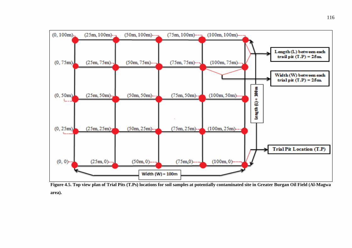
116
Figure 4.5. Top view plan of Trial Pits (T.Ps) locations for soil samples at potentially contaminated site in Greater Burgan Oil Field (Al-Magwa
area).

117
Figure 4.6. Top view plan of Trial Pits (T.Ps) locations for soil samples at potentially non-contaminated site in Greater Burgan Oil Field (Al-
Magwa area).
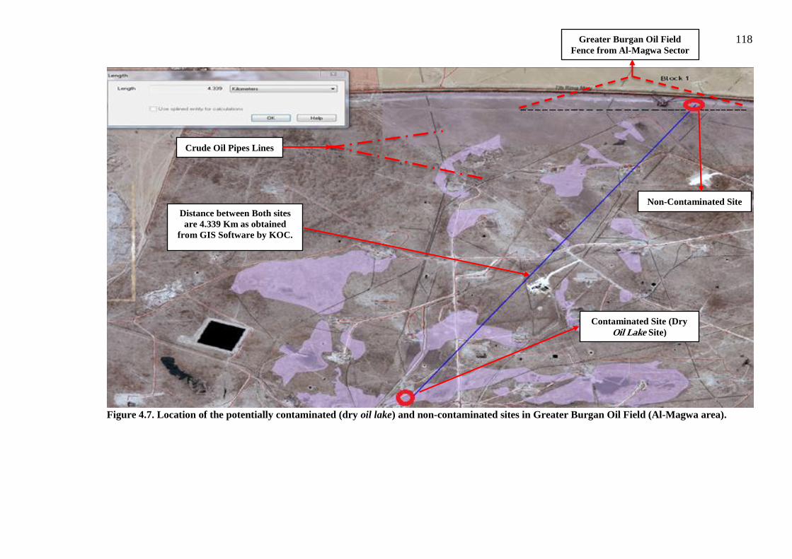
118
Figure 4.7. Location of the potentially contaminated (dry oil lake) and non-contaminated sites in Greater Burgan Oil Field (Al-Magwa area).
Distance between Both sites
are 4.339 Km as obtained
from GIS Software by KOC.
Non-Contaminated Site
Contaminated Site (Dry
Oil Lake Site)
Greater Burgan Oil Field
Fence from Al-Magwa Sector
Crude Oil Pipes Lines

119
4.6 Sampling Methods for Potential Contaminated and Non-Contaminated Sites
The chosen potential contaminated site is close to the Gas Centre (GC-09) and several oil
well pipeline. Some of these had been destroyed during the Iraqi invasion of Kuwait,
consequently the area looked like an old, dry, oil lake. Photographs were obtained from
KOC‟s GIS software (including site coordinates) and Google Earth to indicate the position
of the sampling site. Small coloured flags were used as markers so as to easily locate the
position of Trial Pit Coordinate (T.P.C) within the site before digging and sample
collection commenced.
The non-contaminated site where the samples were taken from, on the other hand, was
relatively clean with some scattered shrubberies and small plants. A photographs was also
obtained from KOC‟s GIS software and Google Earth (including site coordinates) to
indicate the position of the sampling site. The non-contaminated site was located beyond
the KOC‟s security fence. Small, coloured flags were also used as markers to demarcate
the location of T.P.C at the non-contaminated site prior to digging and collection of
samples (Figures 4.8 and 4.9). During this sampling phase, disturbed and undisturbed
samples were taken from both sites.
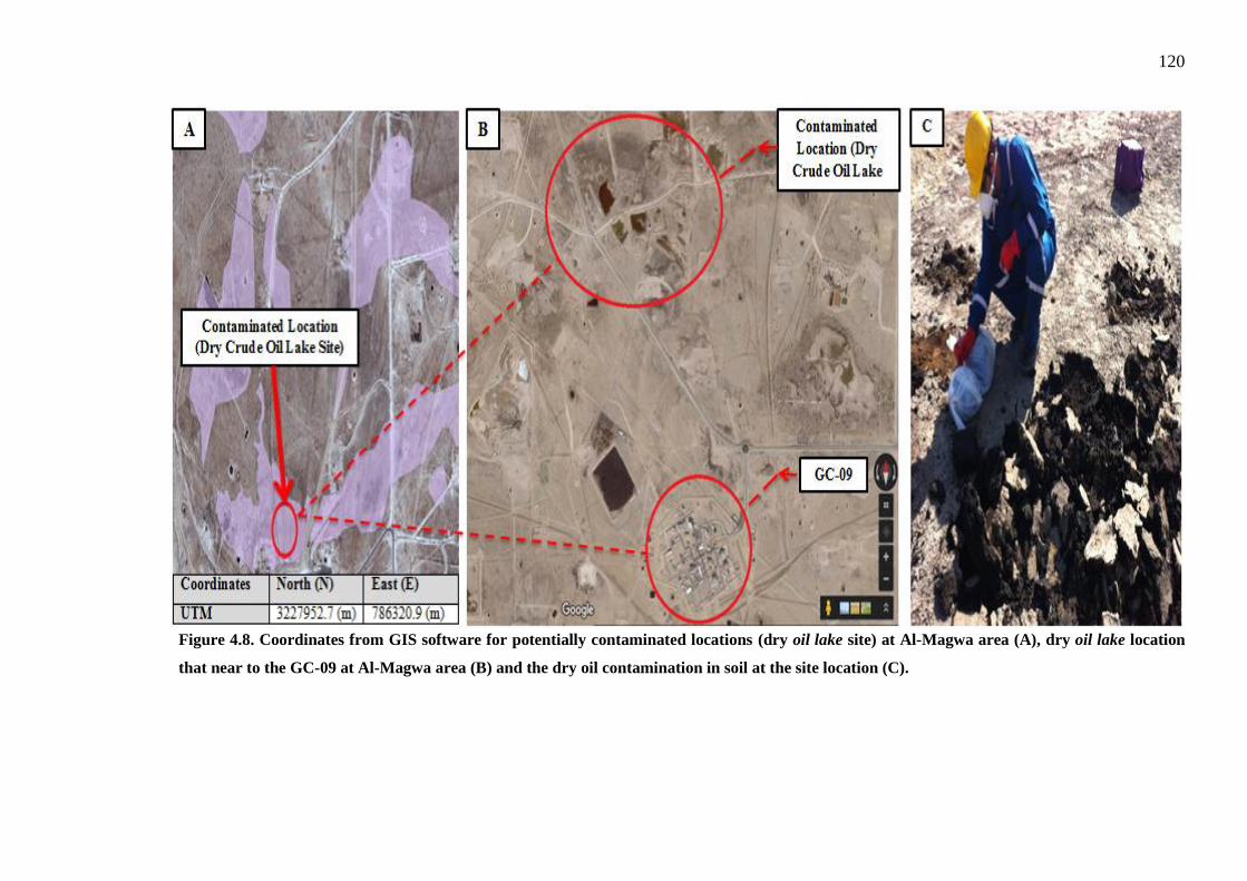
120
Figure 4.8. Coordinates from GIS software for potentially contaminated locations (dry oil lake site) at Al-Magwa area (A), dry oil lake location
that near to the GC-09 at Al-Magwa area (B) and the dry oil contamination in soil at the site location (C).
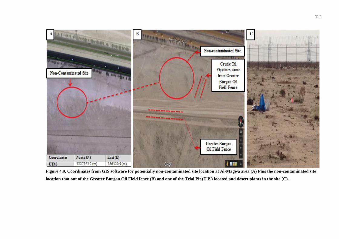
121
Figure 4.9. Coordinates from GIS software for potentially non-contaminated site location at Al-Magwa area (A) Plus the non-contaminated site
location that out of the Greater Burgan Oil Field fence (B) and one of the Trial Pit (T.P.) located and desert plants in the site (C).
122
4.6.1 Disturbed Sampling
Manual digging equipment (chisel and shovel) was used to extract disturbed samples from
several depths (0.0 m, 0.25 m, 0.5 m, 1.0 m, 1.5 m & 2.0 m) below ground level at both
potentially contaminated and non-contaminated sites. All disturbed samples were collected
in plastic bags and carefully sealed with plaster. Each plastic bag was labelled according to
the site name, trial pit coordinate and sample depth. Each plastic bag was labelled
according to the site name, trial pit coordinate and sample depth. They were then
transferred to storage under controlled temperature conditions of 18 C°. This was carried
out according to the sampling preservation method of these studies, i.e. ASTM D 4220-95
(2000) and Landon (2007) (Plate 4.1).
For the purposes of PSD, Atterberg Limits, pH and water soluble Cl-
and (SO3 & SO4) tests, 132 samples, each weighting 2.5 Kg, were
taken from the 22 T.Ps (22 samples from each sampling depth) at the
potentially contaminated site as well as 30 samples collected from the
five T.Ps at the non-contaminated site.
Another 132 samples each weighting 50 g, were taken from the 22 T.Ps
from six different depths (i.e. 0.0 m, 0.25 m, 0.5 m, 1.0 m, 1.5 m and
2.0 m) in the potentially contaminated site, and 10 samples, each
weighting 50 g from two depths of 0.0 m and 0.25 m only, from the
potentially non-contaminated site. Each one of the above samples was
taken for the purpose of the elemental analysis test.
Another 110 samples, each weighting 100 g, were obtained from five
depths of 0.0 m, 0.25 m, 0.5 m, 1.0 m and 1.5 m from the 22 T.Ps in the
potentially contaminated site; 10 samples, each weighting 100 g, were
obtained from two depths of 0.0 m and 0.25 m only, from the
123
potentially non-contaminated site. All the above samples were obtained
for the purpose of the GC-MS test.
All the plastic bag samples collected for the elemental analysis and GC-MS tests were
placed inside conservation (heatproof) boxes and transported to the chemical laboratory at
KISR Ahmadi Branch and stored under 3°C. For the purpose of this test, sampling was
undertaken in the morning (5 a.m.) during the winter season and transported directly by car
(a distance of 19 km) to the laboratory. The U.S. EPA Method 8270D (1998) and Hesnawi
and Adbeib (2013) method was used during the sampling process. Figure 4.10 details the
sampling site and chemical laboratory at KISR Ahmadi.
4.6.2 Undisturbed Sampling
For the Purpose of the Direct Shear test, undisturbed samples were
obtained from different T.Ps at depths of 0.0 m, 0.25 m, 0.5 m, 1.0 m
and 2.0 m. Sampling was undertaken by means of pushing a sharp-
edged stainless steel tube of 25 mm diameter by 45 mm height through
the soil by tamping the tube gently through the soil (ASTM D 2937-04,
2008). The soil inside the tube was trimmed at both top and bottom
sides. The tubes were then secured using rubber cups at the top and
bottom, placed into a plastic bag and sealed with plaster. Bags were
then transferred to the conservation box to be transported directly to the
soil laboratory in order to find the natural density and water content.
The soil was then taken from these tubes and compacted again inside
the shear box to ascertain the natural density and water content as it had
been on the site, in other words, inside the sampling tube. 42 samples
were obtained from the potentially contaminated site and 18 samples
from the potentially non-contaminated site.
124
For the purpose of the permeability test, sampling was undertaken using
the same method as that used for obtaining undisturbed samples inside
the stainless steel sampling ring. The difference being that the sampling
ring size was 50 mm diameter by 50 mm height and that the
permeability test was conducted on the undisturbed sample inside the
sampling ring itself. 24 samples were taken from the potentially
contaminated site while 12 samples were collected from the potentially
non-contaminated site. Plates 4.2 and 4.3 are photographs taken during
the field sampling works (plate A.4.2).

125
Plate 4.1. Soil samples were stored within 18 °C temperatures before transferring to the lab
to be tested for Atterberg Limit, Sieve Analysis, pH and Water soluble Chloride (Cl-) and
Sulphate (SO3 & SO4) contents.
Figure 4.10. Location of the sampling site and chemical laboratory at KISR Ahmadi branch
clarifying the distance between the two locations.
Sampling Location

126
Plate 4.2. Dry oil lake at contaminated site (A), the works of digging at the contaminated site
(B) and the soil profile in the contaminated site (C).
A B
C
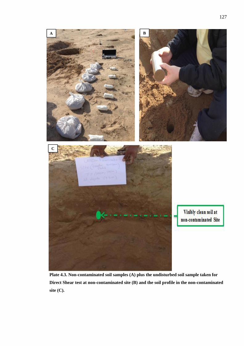
127
Plate 4.3. Non-contaminated soil samples (A) plus the undisturbed soil sample taken for
Direct Shear test at non-contaminated site (B) and the soil profile in the non-contaminated
site (C).
A B
C
128
4.7 Soil Characterisation
This section showing the methodology for the soil characterization of potentially
contaminated and non-contaminated sites will be outlined and classified into aspects, i.e.
geotechnical and geochemical characterisation as well as hydrocarbon pollutants
characterisation.
Geotechnical testing was carried out in order to determine whether dry oil lake residue had
had any significant effect on the geotechnical properties, i.e. physical and strength
properties, of the soil; this was undertaken by comparing the contaminated and non-
contaminated soils. The geochemical testing was carried out to see whether dry oil lake
residue had any influence on the geochemical properties; also performed through a
comparison of the contaminated and non-contaminated soils. The hydrocarbon pollutants
test was carried out to see whether dry oil lake residue had created a chemically aggressive
problem for the environment; this was performed through detecting chemical compositions
of the hydrocarbon pollutants and their concentration in the contaminated soil.
The geotechnical, geochemical and hydrocarbon pollutants‟ analysis of the contaminated
samples collected at the dry oil lake site in the Greater Burgan Oil Field (Al-Magwa area)
was essential to this study as the area will see significant construction and development
over the next five years.

129
4.7.1 Geotechnical Characterisation
As realised from the sample collection phase of this project, the oil spills‟ contamination
was no longer found at depths lower than 2.0 m. Therefore, the investigation was limited to
this depth 2.0 m.
The geotechnical tests carried out for this study included the PSD, Atterberg Limit,
permeability (hydraulic conductivity), Direct Shear and SEM tests. The PSD and
Atterberg Limit test were conducted on samples collected from two sites (contaminated
and non-contaminated), whereas the SEM test was utilised to further investigate the grain
size and shape of the samples. The permeability test (hydraulic conductivity) gave an idea
of the extent of hydrocarbon entrances through the soil layers and of hydrocarbon
contamination migration into the ground water. While the Direct Shear test gave an idea as
to the bearing value of soil which might be affected by hydrocarbon contamination.
The material collected from each site was divided into two portions using a mechanical
splitter. One of these was then shipped to the University of Portsmouth in the UK and
stored in a laboratory for SEM work; the other remained in three laboratories in Kuwait,
including those of INCO in the Sabhan region, SMATCO in the Alrayi region and at the
soil material laboratory in the Kuwait Institute of Scientific Research (KISR) (Figure
A.4.13).
Sieve analyses and Atterberg Limit tests were carried out at the INCO laboratory. The
Direct Shear tests were conducted at the SMATCO laboratory, while the permeability test
took place at the KISR‟s soil laboratory.
130
4.7.1.1 Plasticity
The Atterberg Limit test for Liquid Limits and Plastic Limits were carried out on soil
samples in this study in accordance with the methods described by BS 1377, part 2: 1990:
4.5 and 5.3 (BSI, 1990a), respectively. The laboratory work on this test is shown in Figures
A.4.14, A.4.15 and Plate A.4.3 in Appendix A.
4.7.1.2 Particle Size Distribution (PSD)
The technique known as dry sieving is appropriate for soils with very little content of silt
and clay particles (sizes of less than 6 µm) normally used in the UK under (BSI, 1990a),
therefore, this technique was chosen for this study. Some photographs were taken in the
laboratory showing the author performing this test (Figure A.4.16 and Plate A.4.4).
4.7.1.3. Scanning Electron Microscope (SEM)
The SEM method is regularly used to produce images of shapes of objects (SEI) in high-
resolution to indicate spatial variations in chemical compositions (GIA, n.d.). Thus, SEM
tests were performed to further analyse the distribution of particle sizes in high resolution
images of the sample in an effort to study the effect of the dry oil lake upon the shape of
surface grains. Two samples were tested, one taken from the hydrocarbon contaminated
area and another from the non-contaminated area (Figure A.4.17). This means that multiple
grains for each soil sample (contaminated and non-contaminated) were obtained and
attached to an Aluminium pin stub using a carbon adhesive disk. This was then coated with
a fine coating of Gold/Palladium which was done by using a manual sputter coater.
4.7.1.4 Permeability (Hydraulic Conductivity)
The permeability coefficient test performed on soil samples was undertaken in accordance
with the procedures defined in ISO/TS 17892-11: 2013, with constant-head conditions. For
more details about the test procedures see Table A.4.3 and Plate A.4.5 in appendix A.
131
4.7.1.5 Shear Strength
The Direct Shear tests were performed in accordance with the BSI (1990b) by means of
testing apparatus (MATEST) equipped with a mechanical loading system. All samples
were prepared by compacting a fixed amount of soil in a square shear box with dimensions
of 60 mm x 60 mm and 23 mm thick in order to have the same natural density in the site
(of undisturbed sample).
The soil in the square shearing box was then tested under consolidated drained conditions.
Vertical loads were gradually applied incrementally to provide the required normal
(vertical) stress. Three different normal stresses of 50, 100, 150 kPa were applied during
the test in order to determine the angle of internal friction (φ) of the soil. Each normal
stress was applied for a certain period of time (around 45 minutes), this was required to
ensure the full settlement of the sample. The soil sample was subsequently sheared at a
displacement rate of 0.35 mm/min, during which readings of shear displacements
(horizontal displacement) and shear force were recorded at suitable intervals. Photographs
of the sample tests in the laboratory are illustrated in Plate A.4.6.
4.7.2 Geochemical Characterisation
This section details the geochemical characterisations including: names pH; water soluble
(Cl-, SO3 & SO4); Vario Macro elemental analysis (C %, N %, H % & S %); and GC-MS
(TPH concentration and their compositions). Tests were carried out to establish the
geochemical properties of the potentially contaminated and non-contaminated samples.
The pH test was conducted to determine soil acidity or alkalinity, while the water soluble
Cl-, SO3 and SO4 tests analysed the soils‟ chloride and sulphate content. These chemicals
could lead to chemically aggressive corrosion of concrete and the reinforcements in
reinforced steel particularly in foundation of structures.

132
An elemental analysis test was performed to assess the percentages of carbon (C %),
hydrogen (H %), Nitrogen (N %) and sulphur (S %) in the samples. Meanwhile, the GC-
MS test was carried out to determine the TPH concentration and its chemical composition
in the soil. These tests were conducted in two laboratories in Kuwait, namely the KISR-
Ahmadi branch and the INCO laboratory in Sabhan.
4.7.2.1 Hydrogen Ion Concentration (pH)
The soil pH test in this study was carried out in accordance with the method described by
BS-1377-part 3, 1990 (BSI, 1990c). A 30g mass of each soil sample (contaminated & non-
contaminated) was dried in a drying cabinet at 40 °C for 24 h (Lec, UK). Each sample was
re-weighed and poured into a beaker, 75 mL of distilled water was then added to the
beaker and mixed for 5 minutes by a mechanical stirrer (CP Cole-parmer). The mixture
was allowed to stand for one hour so that most of the suspended materials could settle. The
pH reading was then taken for samples by a pH meter after being calibrated for pH 7. Plate
A.4.7 illustrates the testing procedure undertaken in the laboratory.
4.7.2.2 Water Soluble Chloride (Cl-) and Sulphate (SO3 & SO4) Content
For this study, the tests on soil samples were carried out in accordance with BSI-1377, part
3:1990: 7.2 and 5 (BSI, 1990c).The works laboratory for the water soluble Cl-, SO3 and
SO4 tests are shown in Plate A.4.8.
4.7.2.3 Vario Macro Elemental Analysis (EA)
The elemental analyser test was performed using CHNS in accordance with the Vario
Macro apparatus for soil samples to determine the percentage of carbon, hydrogen,
nitrogen and sulphur content present in the soil. In principle, the operation involved
digestion of samples at very high temperatures of between 800 °C to 1200 °C followed by
scrubbing of non-analytes from the combustion gasses. A Helium career stream was
133
employed to transport the analyte gasses. After the formed nitrogen oxide was reduced, the
gas mixture was separated into its components which were then released to a detector
(TCD) in sequence.
Moreover, percentage contents of the elements were determined from the detector signal
which was linked to the sample weight and the stored calibration curve (The Universal
Way of Macro Analysis, n.d.). The separation of gas was carried out using computer
controlled absorber/desorber tubes specifically designed to absorb the analyse gasses of
H2O, CO2 or SO2 and to release them by increasing the temperature. This resulted in an
immense dynamic concentration and an overlap-free peak separation (The Universal Way
of Macro Analysis, n.d.).
Samples were weighed into 45 mg by electronic scale weight and then well wrapped in
small foil. All the samples prepared for this test, were taken into the sample holder of the
elemental device (1 sample took 20 minutes to test). The samples‟ results (N %, H %, S %
and C %) were presented in a PC computer linked to an elemental device (Plate A.4.9).
4.7.3 Hydrocarbon Characterisation
As explained in Chapter 3 (p.51) by ATSDR, 1999, the term TPH is employed to define a
large group of hundreds of organic compounds derived from crude oil. Although it is
unrealistic to perform measurements on each individual compound, for the purposes of this
study, analysed hydrocarbon pollutant in soil samples has been termed TPH.
4.7.3.1 Hydrocarbon Extraction
In order to extract the hydrocarbon from the soil sample, an Accelerated Solvent Extractor
(ASE350 Dionex) was used (Plate 4.4). The ASE is capable of extracting hydrocarbon
samples in a much shorter time and with a considerably less amount of solvents as
compared with other usual methods such as Sonication and Soxhlet. During this phase, soil
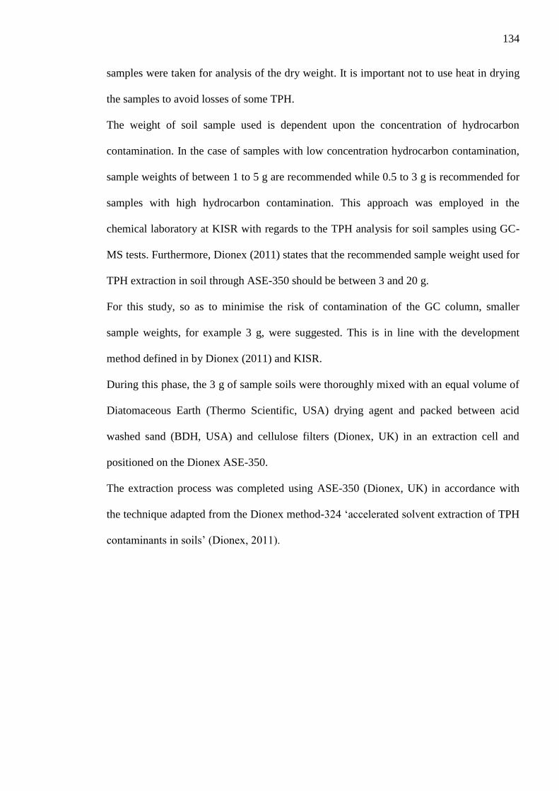
134
samples were taken for analysis of the dry weight. It is important not to use heat in drying
the samples to avoid losses of some TPH.
The weight of soil sample used is dependent upon the concentration of hydrocarbon
contamination. In the case of samples with low concentration hydrocarbon contamination,
sample weights of between 1 to 5 g are recommended while 0.5 to 3 g is recommended for
samples with high hydrocarbon contamination. This approach was employed in the
chemical laboratory at KISR with regards to the TPH analysis for soil samples using GC-
MS tests. Furthermore, Dionex (2011) states that the recommended sample weight used for
TPH extraction in soil through ASE-350 should be between 3 and 20 g.
For this study, so as to minimise the risk of contamination of the GC column, smaller
sample weights, for example 3 g, were suggested. This is in line with the development
method defined in by Dionex (2011) and KISR.
During this phase, the 3 g of sample soils were thoroughly mixed with an equal volume of
Diatomaceous Earth (Thermo Scientific, USA) drying agent and packed between acid
washed sand (BDH, USA) and cellulose filters (Dionex, UK) in an extraction cell and
positioned on the Dionex ASE-350.
The extraction process was completed using ASE-350 (Dionex, UK) in accordance with
the technique adapted from the Dionex method-324 „accelerated solvent extraction of TPH
contaminants in soils‟ (Dionex, 2011).
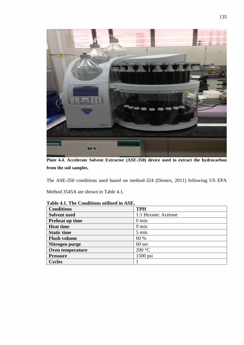
135
Plate 4.4. Accelerate Solvent Extractor (ASE-350) device used to extract the hydrocarbon
from the soil samples.
The ASE-350 conditions used based on method-324 (Dionex, 2011) following US EPA
Method 3545A are shown in Table 4.1.
Table 4.1. The Conditions utilised in ASE.
Conditions TPH
Solvent used 1:1 Hexane: Acetone
Preheat up time 0 min
Heat time 9 min
Static time 5 min
Flush volume 60 %
Nitrogen purge 60 sec
Oven temperature 200 °C
Pressure 1500 psi
Cycles 1
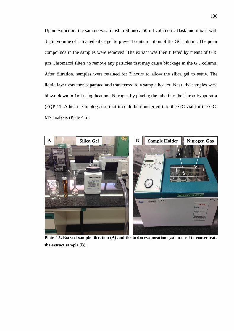
136
Upon extraction, the sample was transferred into a 50 ml volumetric flask and mixed with
3 g in volume of activated silica gel to prevent contamination of the GC column. The polar
compounds in the samples were removed. The extract was then filtered by means of 0.45
µm Chromacol filters to remove any particles that may cause blockage in the GC column.
After filtration, samples were retained for 3 hours to allow the silica gel to settle. The
liquid layer was then separated and transferred to a sample beaker. Next, the samples were
blown down to 1ml using heat and Nitrogen by placing the tube into the Turbo Evaporator
(EQP-11, Athena technology) so that it could be transferred into the GC vial for the GC-
MS analysis (Plate 4.5).
Plate 4.5. Extract sample filtration (A) and the turbo evaporation system used to concentrate
the extract sample (B).
A B Nitrogen Gas Sample Holder Silica Gel

137
4.7.3.2 Gas Chromatograph Mass Spectrometry (GC-MS)
In accordance with Bul, (2008), GC-MS was utilised in mixtures to segregate the volatile
compounds so that they could be quantified and identified. Within this technique, ASE was
employed to extract the petroleum hydrocarbons from solid samples. The extracts were
subsequently analysed using the GC-MS technique.
TPH was further analysed by means of Agilent Technologies (USA) 6890N GC with
5975B MSD, 7683B Automatic liquid sampler and an Agilent HP-5MS (P/N# 19091S-
433) column, in accordance with the methods described in Table 4.2 (Plate 4.6):
Table 4.2. The method used in GC-MS instrument.
GC-MS Instrument Parameters Methods
MS Modes Scan Mode
Software used Agilent MSD Chemstation.
Scan parameters Lower mass 20 m/z.
Higher mass 450 m/z.
Solvent Delay 2 min.
MS Parameters MS-Source 230 °C.
MS-Quad 150 °C.
Multimode injection 2µl in split less mode
Column Used
Agilent HP-5MS (P/N#
19091S-433) 30 m × 250 µm
× 0.25 µm
Temperature
Program
Injector
temperature 220 °C
Oven
Temperature
Initial temperature 60 °C held for 10
minutes and then increased under two
different temperature rate.
Temperature
Rate (1)
Increased 15 °C/minute to 220 °C and
held for 5 minutes.
Temperature
Rate (2)
Increased to 260 °C at the same rates
of 15 °C/minute and held for 5
minutes.
Total Run time 33.33 minutes.

138
Plate 4.6. Agilent Technology 6890N GC with 5975B MSD and 7683B Automatic Liquid
Sampler.
Using the Kuwait Diesel Standard, the TPH calibration peaks were prepared at
concentrations of between 20-1000 µg/ml. A Diesel Range Oil (DRO) which contains
C10-C28 was injected on a regular basis to confirm the retention time repeatability. The
retention time for the area under the peak for the DRO‟s was measured at between 6 and
23 minutes, this area under the peaks was integrated according to standards (Figure 4.13).
A linear regression equation was formed by plotting the calibration peak of diesel in µg/ml
against the area under the peak and this was used to convert the area under the peak into
TPH in µg/ml. This was converted to concentration per dry weight of soil.
Dry Wt
× 100 = Dry Mass (%) (EQ. 4.1)
Wet Wt
Wet Wt. × Dry Mass
= Dry Wt. of Soil (Actual used in ASE) (EQ. 4.2)
100
TPH (µg/ml) obtained from the Integration
× 1000 = TPH of Dry Soil (µg/g) (EQ. 4.3)
Dry Wt. of Soil Used
Agilent
6890N GC Agilent
5975B MSD
Agilent 7683B Automatic liquid Sampler
Agilent
Chemstation
Software
139
4.7.3.3 Unresolved Complex Mixture (UCM)
Hump or unresolved complex mixture (UCM) - as shown in GC-MS chromatograms
(Figure 4.11) - resulted from incomplete degradation of petroleum hydrocarbon in
environmental samples along biogenic organic compounds such as alkanes, steroids,
sterones, fatty alcohols, fatty acids and wax esters. When this chromatogram (Figure 4.13)
is integrated with baseline at retention time for 6 min and to baseline at retention time for
23 min (this method was advised by the (TPHCWG) (1998, p.27)), it was found that the
area under the curve of UCM increased more than for the area under individual spikes.
The chromatograms of DRO could be integrated by either considering only the area under
individual spikes without considering the area in UCM part or by considering both the area
under individual spikes and corresponding area in the UCM part - the latter was followed
in this study. This method has been used in many published papers investigating
environmental samples including those of Muijs and Jonker (2009), Bregnard et al. (1998)
and Wang et al. (1995). This method of analysis was preferential for this study to one
involving the measuring of each peak height due to the lack of distinct peaks found in the
chromatogram during the development of the methodology. The GC-MS method used
during sample testing is presented in detail in Figure A.4.18.
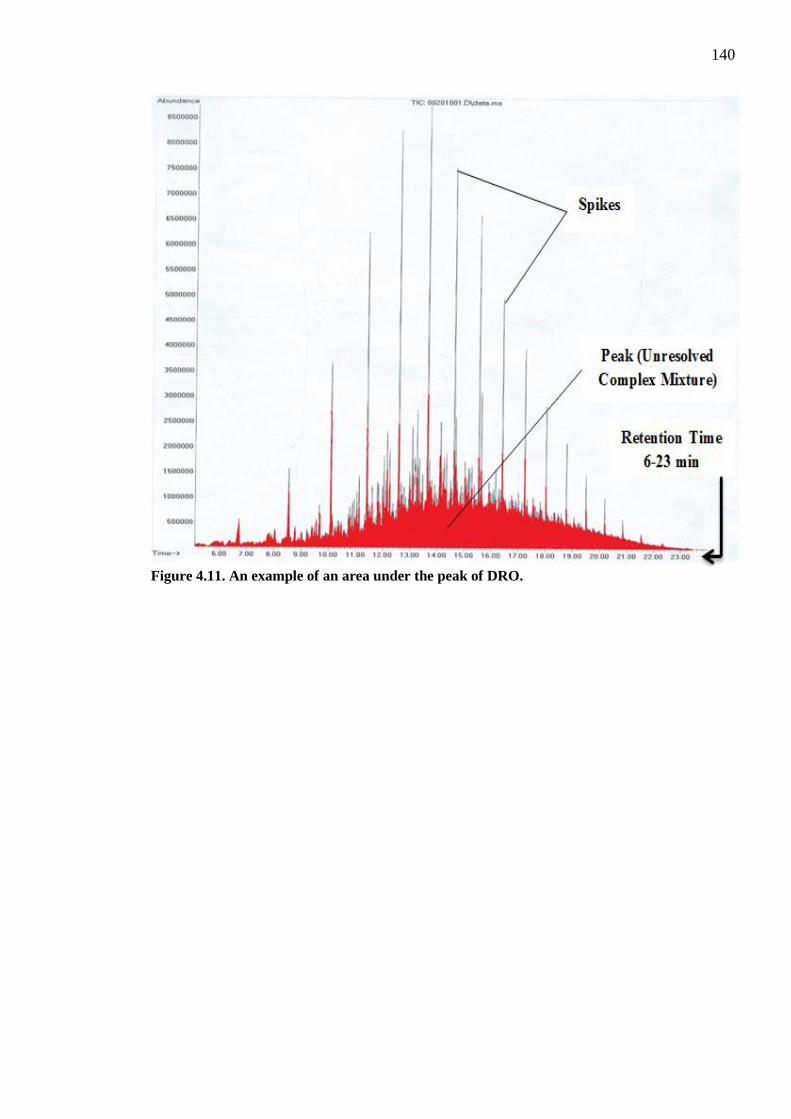
140
Figure 4.11. An example of an area under the peak of DRO.
141
4.8 Statistical Data Analysis
The geotechnical, geochemical and hydrocarbon pollutants characterisation tests data used
in this study were analysed quantitatively using IBM SPSS Statistics (Statistical Package
for the Social Sciences) version 21 using p < 0.05 to define statistical significance. In order
to carry out the statistical analysis, the data analysis framework was first outlined, this was
followed by data classification and then application of the following quantitative tests:
Outlier Testing (Boxplot and Outlier Labeling Rule)
Normality Testing (Shapiro of Normality)
Parametric or Non-Parametric Tests (i.e. T-Test or Mann Whitney U Test)
Linear Regression and Wilcoxon Signed Rank tests.
4.8.1 Data Classification
Soil samples were taken at various depths from two different sites, i.e. contaminated and
non-contaminated sites, for geotechnical, geochemical and hydrocarbon characterisation.
These samples are briefly classified within this sub-section to assess their ability to
confirm the type of statistical analysis tests to be used for the geotechnical, geochemical
and hydrocarbon analysis in this study (Tables 4.3 to 4.5). Therefore the design is a
between-groups study (group 1: contaminated data, group 2: non-contaminated data) with
three test samples (geotechnical, geochemical, and hydrocarbon soil samples). Each to be
taken at six depths: 0.0 m; 0.25 m; 0.5 m; 1.0 m; 1.5 m; and 2.0 m. The comparison
between the mean values (if parametric data) or median values (if non-parametric data)
taken from the contaminated and non-contaminated sites will, therefore, be used for the
statistical analysis.
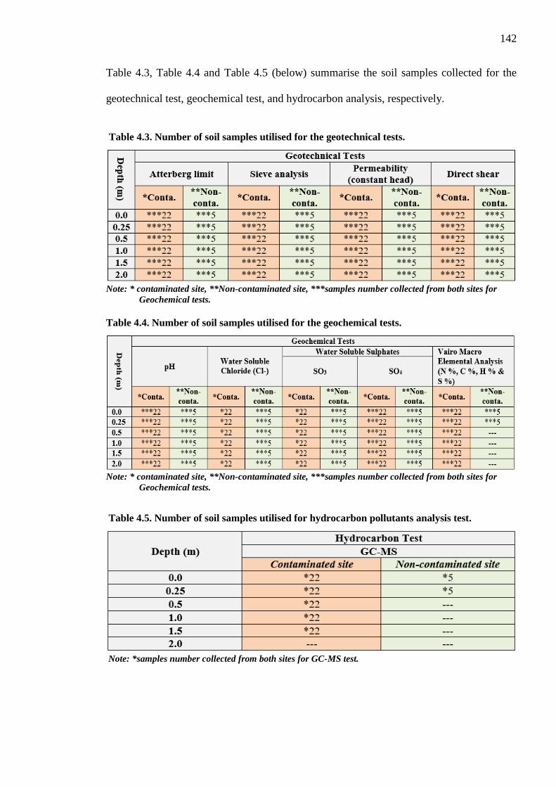
142
Table 4.3, Table 4.4 and Table 4.5 (below) summarise the soil samples collected for the
geotechnical test, geochemical test, and hydrocarbon analysis, respectively.
Table 4.3. Number of soil samples utilised for the geotechnical tests.
Note: * contaminated site, **Non-contaminated site, ***samples number collected from both sites for
Geochemical tests.
Table 4.4. Number of soil samples utilised for the geochemical tests.
Note: * contaminated site, **Non-contaminated site, ***samples number collected from both sites for
Geochemical tests.
Table 4.5. Number of soil samples utilised for hydrocarbon pollutants analysis test.
Note: *samples number collected from both sites for GC-MS test.
143
4.8.2 Outlier Labelling Rule and Normality Tests
Boxplots were initially used to visually search for outliers on each boxplot, after which the
„Labelling Outlier Rule‟ procedure was performed on the data for both contaminated and
non-contaminated sites to identify lower and upper outliers through the use of the
following formula:
Lower outlier values = Q1- (1.5 * (Q3-Q1)) (EQ. 4.4)
Upper outlier values = Q3+ (1.5 * (Q3-Q1)) (EQ. 4.5)
Where Q1 is lower quartile, Q3 is upper quartile (obtained via Quartile, Percentiles in
SPSS), and g is a standard value of 1.5. (Hoaglin et al., 1986) For this procedure, a low
outlier is defined as a value that is lower than the lowest lower outlier; whereas a high
outlier is defined as a value that is higher than the highest upper outlier value. These values
are then looked into the SPSS, descriptives explore, extreme values table. Outliers are
deleted from the dataset.
Prior to statistical analysis, the normality assessment of data is a prerequisite due to the fact
that the normal data is the fundamental assumption for parametric tests. On the other hand,
the non-normal data follows the assumption of a non-parametric test. The numerical
approach is employed mathematically using two primary tests namely Kolmogorov-
Smirnoff (K-S) and Shapiro-Wilk (S-W), the latter is more appropriate for small sample
size ≤ 30 cases. Based on (Storey, n.d.), these tests compare the set of scores in a sample to
a normally distributed set of scores having the same mean and standard deviation. Should
the test prove to be non-significant (i.e. p-value > 0.05 where the p-value obtained from the
software is considered as being significant value of (K-S) & (S-W) tests), this demonstrates
that the data is not considerably different from a normal distribution i.e. the data is
normally distributed. However, in the case the test is found to be significant, i.e. p-value

144
<0.05, the data is not normally distributed (Storey, n.d.). As mentioned by Storey (n.d.)
and Pallant (2005), the S-W test is employed when sample size is small, i.e. less than 100.
4.8.3 Parametric and Non-Parametric Method
The parametric method is typically employed in circumstances where the data follows a
normal distribution (Pallant, 2005) According to Sullivan (2016), the parametric test
includes specific probability distribution or normal distribution. It provides estimation for
the important parameters of the data distribution such as the mean or difference in the
means from the sample data. In contrast, if it is obvious that the data is not normal
distribution, the non-parametric method can be employed instead. As clarified by Sullivan
(2016), the non-parametric test is occasionally termed a distribution-free test as it is based
on fewer assumptions, e.g., they do not consider that the outcome is normally distributed.
As classified by Pallant, (2005) and Kasule (2001), the common statistical tests employed
in parametric and non-parametric methods for the data are as displayed in Table 4.6.
Table 4.6. The tests used for parametric and non-parametric statistics (Source: Pallant,
2005; Kasule, 2001).
State Parametric test Non-Parametric test
One sample z-test, One sample T-Test Sign test
Two independent sample
means/mean ranks/medians
between groups
Independent samples T-Test Wilcoxon Rank Sum Test, Mann
Whitney Test
Two paired sample
means/mean ranks/medians
within groups
Paired T-Test Wilcoxon Signed Rank Test
Three or more independent
sample means/mean
ranks/median between groups
Between Groups ANOVA (one-
way) Kruskall Wallis Test
Multiple comparison of
means/mean ranks/median
within groups
Repeated Measures ANOVA
(compares mean) Friedman Test
145
4.8.3.1 T-Test
The T-Test is a parametric statistical test used to determine whether the mean difference
between two normally distributed groups is statistically significant (Pallant, 2005). It
supports a null hypothesis which specifies that:
H0: the population means of both groups are similar (when the p-value is > 5%).
H1: the population means are significantly different (when the p-value is ≤ 5%).
The T-Test is expressed as:
t(DF) = t-value.
DF = Degrees of Freedom.
P = p-value.
4.8.3.2 Mann-Whitney U Test
The purpose of the non-parametric Mann-Whitney U Test (non-parametric version of the
independent samples T-Test above, Shier, (2004)) is to assess whether two independent
groups differ significantly in some dependent variable, which is either ordinal or
continuous, or whether the data is not normally distributed (Field, 2009).
Its purpose is to test the null hypothesis for two samples which come from the same
population, i.e. have the same median, or alternatively, whether observations in one sample
are inclined to be greater than observations in the other. It compares two distributions
across their mean ranks, rather than mean values. While it is regarded as a non-parametric
test, it still considers that both distributions have a similar shape.
The hypotheses assumed in Mann-Whitney U test are:
H0: the population medians are similar (used if the p-value > 5%).
H1: the population medians are significantly different (used if the p-value ≤ 5%).
146
4.8.3.3 Wilcoxon Signed Rank Test
According to Voraprateep (2013), the Wilcoxon signed-rank test is a rank based alternative
to the parametric T-Test where the distribution of differences within pairs is symmetrical
without the need for normal distribution (Oyeka and Ebuh, 2012). Shaw et al. (2000),
reiterated that this assumption for normal distribution is not considered in the Wilcoxon
signed rank test as the test is based on the rank order of differences instead of the actual
mean differences value. Nonetheless, it is still required to assume that the distribution of
the differences is symmetric.
The hypotheses assumed in Wilcoxon Signed Rank Test are:
H0: the population medians are similar (used if the p-value > 5%).
H1: the population medians are significantly different (used if the p-value ≤ 5%).
4.8.3.4 Regression Analysis
Linear regression analysis was used to investigate and model the relationship between a
response variable (dependent variable) and one or more predictor variables, to determine
the contribution of response variable(s) to the dependent variable (outcome in a
scatterplot), the predictor is displayed on the x-axis and the response variable on the y-axis.
A line of best fit can be added to show the direction of the relationship, and the accuracy of
the prediction based on the R Square value, which shows how the actual data fits the
predicted data values along the regression line. The linear regression equation is expressed
as (Yates, 2012):
m = slope or gradient
c = the y intercept
Linear regression is based on the assumption that the data is normally distributed.
Additional assumptions to assess model fit include multi-collinearity (multiple predictors
should not be correlated highly above .8); independence of errors (assessed using Durbin

147
Watson statistic which should be below 2); normality of residuals (errors) assessed via
histogram of residuals; homogeneity of variance (assessed via plot of residuals), and
Cook‟s maximum distance values in residual diagnostics (which should be below 1) (Field,
2009). Regression analysis produces three key statistics to assess model fit: The R Square
value, which indicates how much variation in the dependent variable is explained by the
predictor(s). The F statistic, which indicates the overall fit of the model, which should be
significant. The regression coefficients (unstandardized B and standardised Beta values)
indicate the unique contribution of each predictor on the dependent variable scores.
4.8.4 Analysis Framework
The following analysis framework was developed to test the geotechnical and geochemical
data in a logical fashion, starting with the geotechnical data, followed by geochemical data:
Step 1 – Screen data for outliers using boxplots and Labelling Outlier Rule procedure.
Step 2 –The Shapiro of normality was used to assess whether the assumption of normality
was met for all distributions. When the assumption of normality was violated, non-
parametric statistics were performed on the data.
Step 3 – Perform an independent sample‟s T-Test or Mann Whitney U Test, depending on
the normality of the data, to compare the mean or median difference between the
contaminated and non-contaminated site data groups at six different depths. These tests
were used to determine the significant difference of the soil properties in terms of their
geotechnical and geochemical properties.
Step 4 – If data violates the assumption of normality, perform a non-parametric Wilcoxin
Signed Ranks test to compare soil properties in terms of their geotechnical and
geochemical properties across six different depths within each contaminated and non-

148
contaminated site, to examine whether relationships exist between the property values
across six different depths.
Step 5 – If the data is normally distributed and the above T-Test is significant, perform
linear regression to compare soil properties in terms of their geotechnical and geochemical
properties across six different depths within each contaminated and non-contaminated site,
so as to predict relationships between property values and depth.
4.9 Summary
After detailing the: experimental programme; selecting the tentative site; detailing the
location of the eventual site (Greater Burgan Oil Field – Al Magwa area); final soil
sampling for both contaminated and non-contaminated sites; appraising the appropriate
geotechnical and geochemical tests; and performing required technical procedures for these
tests (geotechnical and geochemical); for the two selected sites at the Al- Magwa area, the
properties of the soils at the contaminated and non-contaminated sites can then be
characterised.
It is imperative to make a note at this juncture that the conducted tests were more relevant
and precise thus delivering more detailed and accurate results. Statistical tests‟ analyses
were conducted in order to support robustness of the results. Further details and outcomes
of geotechnical and geochemical characterisation for the soil samples, obtained from both
the contaminated and non-contaminated sites, as described in this study, will be provided
in Chapters 5 and 6 respectively.

149
5. GEOTECHNICAL CHARACTERISATION
5.1 Introduction
This Chapter presents the findings of the geotechnical characteristics of soil samples taken
from two different locations of the contaminated (dry oil lake) and non-contaminated sites
(see sections (4.5.1 and 4.5.2)). Both these sites are located at the Greater Burgan Field
(Al-Magwa area). It also discusses the main outcomes and shows how the study objectives
have been addressed by linking the experimental findings with several studies in the
literature. Finally, the chapter will give a statistical analysis of the geotechnical
characterisations of the soil samples thus supporting the findings of this work.
The geotechnical characterisation results in this chapter include: the Atterberg Limit; PSD;
SEM; permeability (Hydraulic Conductivity); and Direct Shear tests.
The test results showing similar tables and figures will be put into appendix B; those with
only limited tables and figures will be shown in this chapter as an example or
representative.
5.2 Plasticity
As expected, the findings show that the hydrocarbon contamination has no effect on the
Atterberg limits because the soil was originally silty sand (non-plastic). These results are in
line with various past studies, e.g. Alhassan and Fagge (2013), for example who mixed
clean sand samples with different amounts of 2 %, 4 % and 6 % - by weight - of the crude
oil. Their analysis results showed that the sand samples consistently demonstrated non-
plastic behaviour.
On the other hand, studies carried out by Khamehchiyan et al. (2007), Rahman et al.
(2010) and Pandey and Bind (2014) concluded that for fine-grained soils such as clays and
alluvium, hydrocarbon contamination reduced both their liquid and plastic limits.

150
Since the petroleum material (both at liquid or other phases) is known to be hydrophobic
the consistency of the contaminated soil would not change the plasticity of soil if it was
originally non-plastic (before contamination).
5.3 Particle Size Distribution (PSD)
5.3.1 Laboratory Results of PSD
The results of PSD for soil samples taken from the contaminated dry oil lake are shown in
figures 5.1 and B.5.1, while figures 5.2 and B.5.2 display the results for the non-
contaminated soil samples from the non-contaminated site.
Due to the significant number of curves representing samples taken from many Trial Pit
Coordinates (T.P.Cs) - which are all drawn in each figure, where each figure represents
one depth - the curves interfered in-between these figures and did not become clear
enough. Therefore, only the extreme PSD are represented clearly and are shown by
different colours.
Tables B.5.1, B.5.2, B.5.3, B.5.4, B.5.5 and B.5.6 in appendix B, show the percentages of
each soil class as part of the soil sample corresponding to the position of the T.P.Cs of the
contaminated site (dry oil lake) at different depths, i.e. 0.0 m, 0.25 m, 0.5 m, 1.0 m, 1.5 m
and 2.0 m respectively. Similarly, the percentages of each soil class part against the
position of the T.P.Cs of non-contaminated soil samples at the respective depths mentioned
above are indicated in tables B.5.7, B.5.8, B.5.9, B.5.10, B.5.11 and B.5.12 Furthermore,
the final column of the above tables shows the soil group of the whole sample according to
(BS 1377: Part 2:1990:9.2).The minimum and maximum values of each soil class part
found in the samples representing the same depth are recorded in the above mentioned
tables. The mean and standard deviation values of each soil class part were also calculated
and listed in these tables.

151
From the resulting PSD, curves of the contaminated site (figures 5.1 and (B.5.1)), it was
noted that there were wide ranges in the gradation of soil samples taken from the same
depth but from different locations (T.P.C). It was particularly evident in the top soil (figure
5.1 at depth 0.0 m). However, although this range is still wide it becomes narrower at other
depths (Figures 5.1 and B.5.1. at depths 0.5 m & 2.0 m). From this behaviour it is expected
(logically) that the hydrocarbon contamination is higher in the top soil.
In the non-contaminated area (figures 5.2 and B.5.2), it was noted that (at one depth), the
gradation range between a sample taken from one T.P.C and another is smaller than in the
corresponding contaminated site. Furthermore, the gradation does not vary much with
depth.
The wide ranges in PSD of contaminated soil samples with hydrocarbon taken from the
same depth but from different pit locations (different T.P.C) may be related to the
differences in the ground level of the contaminated oil spill lake caused by higher oil spill
depths leading to higher oil contents at the low ground level of the oil lake during the
earlier stages (before dryness of the lake).
Table (5.1) shows the mean calculated percentage values of soil class as apart from all soil
samples taken from the same depth. The table illustrates a comparison between the two
sites (contaminated and non-contaminated). From the Table, it should be noted that the
mean small grain size percentage values (passing No. #230) for the samples taken from the
contaminated site are all slightly higher than for samples taken from the non-contaminated
site. The larger fraction is due to the drying of hydrocarbon in the contaminated area
forming small, asphaltane particles, as will be explained in sub-section 8.2.1 (see chapter 8,
section 8.2.1).

152
According to the Unified Classification System (Casagrande, 1948), the soil could be
classified as well graded when the uniformity coefficient (Cu) is more than 6.00 and the
coefficient of curvature (Cc) is more than 1.0. Table (5.1) and figures (5.4 and 5.5) further
show that both the Cu and Cc values clearly differ between the contaminated and non-
contaminated sites. The Cu of the top soil at depths (0.0 m and 0.25 m) of both
contaminated and non-contaminated sites were more than six; this is the first requirement
for soil to be classed as well graded. However, in the contaminated site only it drops to
values much lower than six at lower depths. On the other hand, Cu values in the non-
contaminated soil were still higher than six or nearly equal to six - at lower depths.
The second requirement, in respect of Cc is to be between one and three for the well
graded soil; thus it can be seen that all values of Cc for the contaminated soil at all tested
depths were less than one. One the other hand, Cc values were more than one at depths of
0.0 m, 0.25 m and 0.5 m for the non-contaminated soil. Cc however drops to less than one
at deeper levels. This means that the PSD of soil tends to be poorer at lower depths in the
non-contaminated site. It can also be seen from the above that contamination changed the
soil (at least the top soil from 0.0 m to 0.5 m) class from well graded to poorly graded. This
behaviour proves what is shown in section 6.5, i.e. that hydrocarbon was detected down to
0.5 m from ground level.
Furthermore, figure 5.3 shows that the grain size distribution of the non-contaminated site
does not change much with the depth, but in the contaminated site there is a considerable
change with the depth. The two mechanisms (particle aggregation by hydrocarbon
cementation and hydrocarbon residues) are responsible for the differences in PSD curves
of contaminated and non-contaminated soils.
Several studies of hydrocarbon contaminated soils have shown a correlation between
hydrocarbon contamination and grain size distribution. Caravaca and Roldan (2003, p.56)

153
studied clay loam sand contaminated by oil sludge, they showed that the clay content of
these soil samples decreased considerably from 33.3 % to 21.3 % while the silt content
decreased only slightly from 21.7 % to 20.5 % while the content of sand increased from 45
% to 58 %. This change in the constituent content changed the classification of the soil
from clay loam to sandy clay loam. Meegoda and Ratnaweera (1995) found that the
addition of 3 % and 6 % oil to clay soil reduced the clay fraction from 96 % to 87 % and
87 % to 84 % respectively, indicating an increase in soil aggregation with the addition of
the oil.
A study by Gupta and Srivastava (2010) on non-contaminated soils and soil samples
artificially mixed with used engine oil for CL and CH, showed that the size of grains of the
soil-contaminant mixes increases in tandem with the increase in oil content.

154
At depth (0.0 m)
At depth (0.5 m)
At depth (2.0 m)
Figure 5.1. PSD curves for contaminated samples at depths (0.0 m, 0.5 m & 2.0 m).

155
At depth (0.0 m)
At depth (0.5 m)
At depth (2.0 m)
Figure 5.2. PSD curves for non-contaminated samples at depth (0.0 m, 0.5 m & 2.0 m).

156
Table 5.1. Comparing mean values of soil classification constituents between contaminated and non-contaminated samples at six different depths
of 0.0 m, 0.25 m, 0.5 m, 1.0 m, 1.5 m & 2.0 m.
Depth
(m)
Samples
Classification
Mean Percentages Value Exact Soil Percentage
Passing No. (#230)
Grading Analysis (Casagrande, 1948)
Soil Group
(BSI-1377:Part 2:1990a)
Silty/clay%
Fine sand %
Medium Sand
%
Coarse Sand
%
Gravel %
Coefficient of Uniformity (Cu)
Coefficient of Curvature (Cc)
0.0 m Contaminated 10.00 28.00 25.00 17.00 11.00 9.70 8.10 0.90 S-M Non-Contaminated 7.00 22.00 40.00 24.00 1.00 6.60 6.08 1.28 S-M
0.25 m Contaminated 11.00 30.00 30.00 17.00 4.00 10.50 6.41 0.88 S-M Non-Contaminated 8.00 23.00 37.00 22.00 2.00 8.00 6.53 1.18 S-M
0.5 m Contaminated 9.00 40.00 25.00 16.00 3.00 9.50 5.40 0.85 S-M Non-Contaminated 8.00 23.00 39.00 20.00 3.00 8.20 6.71 1.34 S-M
1.0 m Contaminated 8.00 49.00 21.00 14.00 2.00 7.90 3.48 0.95 S-M Non-Contaminated 7.00 26.00 36.00 22.00 1.00 7.40 6.71 0.93 S-M
1.5 m Contaminated 8.00 45.00 20.00 17.00 3.00 7.80 4.12 0.89 S-M Non-Contaminated 7.00 28.00 34.00 22.00 3.00 7.00 6.62 0.87 S-M
2.0 m Contaminated 8.00 46.00 21.00 17.00 3.00 7.80 4.12 0.86 S-M Non-Contaminated 7.00 27.00 40.00 19.00 2.00 6.60 5.87 0.93 S-M

157
Table 5.2. Mean value of the sieve analysis result for contaminated and non-contaminated samples at six different of 0.0 m, 0.25 m, 0.5 m, 1.0 m, 1.5
m, and 2.0 m).
Note; *Conta: Contaminated samples. **Control: Non-Contaminated samples.
B.S. SIEVE
mm
B.S. SIEVE (in/#)
Mean Percent Passing
value for *conta.
sample at depth (0.0
m)
Mean Percent Passing
value for **control sample at depth (0.0
m)
Mean Percent Passing
value for *conta.
sample at depth
(0.25 m)
Mean Percent Passing
value for **control sample at
depth (0.25 m)
Mean Percent Passing
value for *conta. sample
at depth (0.5 m)
Mean Percent Passing
value for **control sample at depth (0.5
m)
Mean Percent Passing
value for *conta. sample
at depth (1.0 m)
Mean Percent Passing
value for **control sample at depth (1.0
m)
Mean Percent Passing
value for *conta.
sample at depth (1.5
m)
Mean Percent Passing
value for **control sample at depth (1.5
m)
Mean Percent Passing
value for *conta.
sample at depth (2.0
m)
Mean Percent Passing
value for **control sample at
depth (2.0 m)
37.6 (11/2") 100.00 100.00 100.00 100.0 100.00 100.00 100.00 100.00 100.00 100.00 100.00 100.00 25.0 ( 1") 99.40 100.00 99.60 100.00 100.00 98.90 100.00 100.00 100.00 100.00 100.00 100.00 14.0 ( 3/5") 97.20 100.00 99.20 99.60 99.80 98.60 99.80 100.00 100.00 100.00 99.80 100.00 10.0 ( 3/8") 95.10 100.00 98.90 99.20 99.50 98.30 99.70 99.90 99.80 99.80 99.30 99.80 6.3 ( 1/4'') 92.30 99.60 98.20 98.70 99.10 98.10 99.40 99.70 99.10 99.20 98.70 99.40
5.00 ( #5) 91.00 99.20 97.70 98.40 98.70 97.90 99.10 99.40 98.60 98.80 98.30 99.20 3.35 ( #6) 88.60 98.80 96.10 97.60 97.40 97.00 98.20 98.60 97.30 97.30 97.10 98.30 2.00 ( #10 ) 80.40 92.70 87.80 90.90 90.40 89.60 92.50 92.00 90.20 91.50 91.50 92.60 1.18 ( #16 ) 72.50 84.90 80.40 84.60 82.20 83.40 84.30 85.90 79.80 83.90 81.10 85.50
0.600 ( #30 ) 63.50 69.00 70.90 68.90 74.20 70.00 78.30 69.90 73.00 69.30 74.20 73.60 0.425 ( #40 ) 56.00 54.30 61.70 53.90 66.80 55.70 73.10 56.20 68.30 55.40 69.40 58.60 0.300 ( #50 ) 46.80 39.30 50.50 40.00 58.00 40.40 65.90 43.30 61.60 44.00 62.30 44.00 0.212 ( #70 ) 38.10 28.50 40.70 31.50 49.60 30.70 56.90 33.80 53.20 35.00 53.40 34.00 0.150 ( #100 ) 27.50 20.20 30.70 23.50 34.20 22.90 38.60 25.20 36.40 25.40 36.40 23.90 0.063 (#230) 9.70 6.60 10.50 8.00 9.50 8.20 7.90 7.40 7.80 7.00 7.80 6.60

158
Figure 5.3. Mean values of PSD for contaminated (brown colour) and non-contaminated (green colour) samples at six different depths of
0.0 m, 0.25 m, 0.5 m, 1.0 m, 1.5 m and 2.0 m.
6.3
5.0
3.35 2.0 1.18 0.6
0.425
0.3 0.15 0.063 10.0
14.0
0.212
0
10
20
30
40
50
60
70
80
90
100
0.001 0.01 0.1 1 10 100 1000
Per
cent
age
Pas
sing
Particle size (in mm)
Mean Value (0.0m)
Mean Value (0.25m)
Mean Value (0.5m)
Mean value (1.0m)
Mean Value (1.5m)
Mean Value (2.0m)
Mean Value (0.0m)
Mean Value (0.25m)
Mean Value (0.5m)
Mean Value (1.0m)
Mean Value (1.5m)
Mean Value (2.0m)
BS sieve aperture size, mm BS sieve aperture size, mm BS sieve aperture size, mm BS sieve aperture size, mm
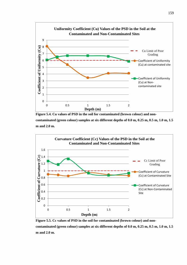
159
Figure 5.4. Cu values of PSD in the soil for contaminated (brown colour) and non-
contaminated (green colour) samples at six different depths of 0.0 m, 0.25 m, 0.5 m, 1.0 m, 1.5
m and 2.0 m.
Figure 5.5. Cc values of PSD in the soil for contaminated (brown colour) and non-
contaminated (green colour) samples at six different depths of 0.0 m, 0.25 m, 0.5 m, 1.0 m, 1.5
m and 2.0 m.
0
1
2
3
4
5
6
7
8
9
0 0.5 1 1.5 2
Coe
ffic
ient
of
Uni
form
ity
(Cu)
Depth (m)
Uniformity Coefficient (Cu) Values of the PSD in the Soil at the Contaminated and Non-Contaminated Sites
Coefficient of Uniformity(Cu) at contaminated site
Coefficient of Uniformity(Cu) at Non-contaminated site
Cu Limit of Poor Grading
0
0.2
0.4
0.6
0.8
1
1.2
1.4
1.6
0 0.5 1 1.5 2
Coe
ffic
ient
of
Cur
vatu
re (
Cc)
Depth (m)
Curvature Coefficient (Cc) Values of the PSD in the Soil at the Contaminated and Non-Contaminated Sites
Coefficient of Curvature(Cc) at Contaminated Site
Coefficient of Curvature(Cc) at Non-ContaminatedSite
Cc Limit of Poor Grading
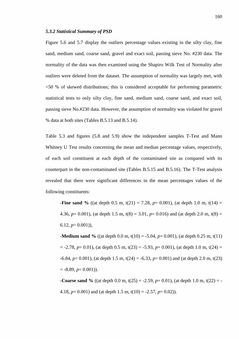
160
5.3.2 Statistical Summary of PSD
Figure 5.6 and 5.7 display the outliers percentage values existing in the silty clay, fine
sand, medium sand, coarse sand, gravel and exact soil, passing sieve No. #230 data. The
normality of the data was then examined using the Shapiro Wilk Test of Normality after
outliers were deleted from the dataset. The assumption of normality was largely met, with
<50 % of skewed distributions; this is considered acceptable for performing parametric
statistical tests to only silty clay, fine sand, medium sand, coarse sand, and exact soil,
passing sieve No.#230 data. However, the assumption of normality was violated for gravel
% data at both sites (Tables B.5.13 and B.5.14).
Table 5.3 and figures (5.8 and 5.9) show the independent samples T-Test and Mann
Whitney U Test results concerning the mean and median percentage values, respectively,
of each soil constituent at each depth of the contaminated site as compared with its
counterpart in the non-contaminated site (Tables B.5.15 and B.5.16). The T-Test analysis
revealed that there were significant differences in the mean percentages values of the
following constituents:
-Fine sand % ((at depth 0.5 m, t(21) = 7.28, p= 0.001), (at depth 1.0 m, t(14) =
4.36, p= 0.001), (at depth 1.5 m, t(8) = 3.01, p= 0.016) and (at depth 2.0 m, t(8) =
6.12, p= 0.001)),
-Medium sand % ((at depth 0.0 m, t(10) = -5.04, p= 0.001), (at depth 0.25 m, t(11)
= -2.78, p= 0.01), (at depth 0.5 m, t(23) = -5.93, p= 0.001), (at depth 1.0 m, t(24) =
-6.84, p= 0.001), (at depth 1.5 m, t(24) = -6.33, p= 0.001) and (at depth 2.0 m, t(23)
= -8.89, p= 0.001)).
-Coarse sand % ((at depth 0.0 m, t(25) = -2.59, p= 0.01), (at depth 1.0 m, t(22) = -
4.18, p= 0.001) and (at depth 1.5 m, t(10) = -2.57, p= 0.02)).

161
-Exact soil passing sieve No. #230 ((at depth 0.0 m, t(23) = 3.70, p= 0.001) and (at
depth 0.25 m, t(18) = 3.28, p= 0.004)).
However, there were no significant differences between the sites in mean percentage
values of the following constituents:
-Silty clay % (at each of the six different depths).
-Fine sand % (at 0.0 m and 0.25 m).
-Coarse % (at 0.25 m, 0.5 m and 2.0 m).
-Exact soil passing sieve No. #230 (at 0.5 m, 1.0 m, 1.5 m and 2.0 m).
A non-parametric Mann Whitney U test showed significant differences in the median
values of gravel between the sites at depth of only 0.0 m (Z= -2.06, U= 20.00, p= 0.04) and
0.25 m (Z= -2.24, U= 12.00, p= 0.03). Nevertheless, no significant differences were found
at depths of 0.5 m, 1.0 m, 1.5 m and 2.0 m.
These above results indicate that the hydrocarbon contamination has a significant effect on
the general PSD of soil which confirms the explanation in the previous section (5.3.1).
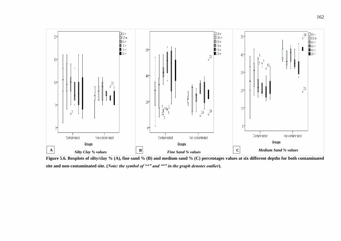
162
Silty Clay % values
Fine Sand % values
Medium Sand % values
Figure 5.6. Boxplots of silty/clay % (A), fine sand % (B) and medium sand % (C) percentages values at six different depths for both contaminated
site and non-contaminated site. (Note: the symbol of “*” and “°” in the graph denotes outlier).
A B C
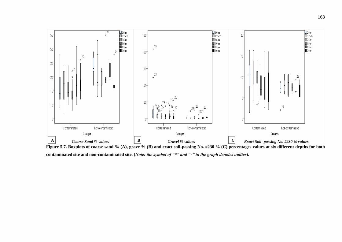
163
Coarse Sand % values
Gravel % values
Exact Soil- passing No. #230 % values
Figure 5.7. Boxplots of coarse sand % (A), grave % (B) and exact soil-passing No. #230 % (C) percentages values at six different depths for both
contaminated site and non-contaminated site. (Note: the symbol of “*” and “°” in the graph denotes outlier).
A B C

164
Table 5.3. Indicates the significant differences of soil classification constituents at six different depths
between contaminated and non-contaminated sites. (Note: outlier values were deleted in this table).
Depth (m) Variable
Site Name N Mean Median SD Min Max Z U t-value p-value
0.0 m
Silty/Clay%
Conta.** 22 9.86 10.50 4.09 1.00 16.00 ------ ------
2.09
0.06
Non-
conta*** 5 6.60 7.00 2.88 2.00 9.00
Fine Sand%
Conta.** 22 27.41 28.50 13.49 1.00 54.00 ------ ------ 1.56 0.13 Non-
conta*** 5 22.00 22.00 4.30 17.00 28.00
Medium Sand%
Conta.** 22 25.82 25.00 8.51 4.00 39.00 ------ ------ -5.04 0.001* Non-
conta*** 5 40.4 38.00 5.03 36.00 48.00
Coarse Sand%
Conta.** 22 16.18 14.00 5.96 9.00 28.00 ------ ------ -2.59 0.01* Non-
conta*** 5 23.60 23.00 4.67 17.00 29.00
Gravel% Conta.** 22 5.45 4.00 4.97 0.00 15.00
-2.06 20.00 ------ 0.04* Non-conta*** 5 1.00 1.00 1.00 0.00 2.00
Exact soil passing No.
#230
Conta.** 22 10.00 10.45 4.11 1.50 16.40 ------ ------ 3.70 0.001* Non-
conta*** 5 7.80 7.95 1.23 6.30 9.00
0.25 m
Silty/Clay%
Conta.** 22 10.41 9.50 3.54 4.00 16.00 ------ ------
1.98
0.07
Non-
conta*** 5 8.00 8.00 2.12 6.00 11.00
Fine Sand%
Conta.** 22 29.14 33.00 14.31 8.00 56.00 ------ ------
0.96
0.36
Non-
conta*** 5 23.40 31.00 11.37 10.00 33.00
Medium Sand%
Conta.** 22 29.64 31.00 8.32 17.00 43.00 ------ ------ -2.78 0.01* Non-
conta*** 5 37.2 36.00 4.60 32.00 42.00
Coarse Sand%
Conta.** 22 16.82 17.50 5.32 7.00 24.00 ------ ------ -1.70 0.10* Non-
conta*** 5 21.80 18.00 8.35 13.00 33.00
Gravel% Conta.** 22 2.31 1.00 2.05 0.00 8.00
-2.24 12.00 ------ 0.03* Non-conta*** 5 0.50 0.50 0.57 0.00 1.00
Exact soil passing No.
#230
Conta.** 22 9.82 9.75 2.09 5.20 13.90 ------ ------ 3.28 0.004* Non-
conta*** 5 8.14 7.90 2.57 5.30 10.60
0.5 m
Silty/Clay%
Conta.** 22 9.85 10.00 2.03 5.00 14.00 ------ ------
1.56
0.13
Non-
conta*** 5 8.20 9.00 2.59 5.00 11.00
Fine Sand%
Conta.** 22 44.83 44 5.81 33 56 ------ ------
7.28
0.001*
Non-
conta*** 5 22.60 25 6.91 12 30
Medium Sand%
Conta.** 22 22.70 21.00 5.68 16.00 36.00 ------ ------ -5.93 0.001* Non-
conta*** 5 39.40 41.00 5.32 32.00 45.00
Coarse Sand%
Conta.** 22 15.64 14.50 4.22 10.00 24.00 ------ ------ -1.79 0.08 Non-
conta*** 5 19.40 22.00 4.28 13.00 23.00
Gravel% Conta.** 22 1.50 1.00 1.73 0.00 6.00
-1.05 27 ------ 0.34 Non-conta***
5 0.75 0.00 1.50 0.00 3.00
Exact soil passing No.
#230
Conta.** 22 9.82 9.90 2.09 5.20 13.90 ------ ------ 0.88 0.41 Non-
conta*** 5 8.14 8.70 2.57 5.30 10.60
Note: *p < .05 indicates to the significant difference in the variables between two different groups. ** Contaminated site. *** Non-contaminated site.
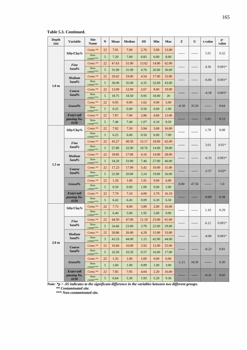
165
Table 5.3. Continued.
Depth (m) Variable Site
Name N Mean Median SD Min Max Z U t-value p-value
1.0 m
Silty/Clay%
Conta.** 22 7.91 7.00 2.76 5.00 13.00 ------ ------
1.01
0.32
Non-
conta*** 5 7.20 7.00 0.83 6.00 8.00
Fine Sand%
Conta.** 22 47.63 51.00 13.62 14.00 62.00 ------ ------ 4.36
0.001*
Non-
conta*** 5 31.00 31.00 4.76 26.00 36.00
Medium Sand%
Conta.** 22 20.62 19.00 4.54 17.00 33.00 ------ ------ -6.84 0.001* Non-
conta*** 5 36.00 35.00 4.35 32.00 43.00
Coarse Sand%
Conta.** 22 13.00 12.00 2.67 8.00 19.00 ------ ------ -4.18 0.001* Non-
conta*** 5 18.75 18.50 0.95 18.00 20
Gravel% Conta.** 22 0.95 0.00 1.62 0.00 5.00
-0.58 35.50 ------ 0.64 Non-conta***
5 0.25 0.00 0.50 0.00 1.00
Exact soil passing No.
#230
Conta.** 22 7.87 7.00 2.86 4.60 13.00 ------ ------ 1.61 0.12 Non-
conta*** 5 7.40 7.40 1.07 6.10 8.50
1.5 m
Silty/Clay%
Conta.** 22 7.82 7.50 3.94 3.00 16.00 ------ ------
1.79
0.08 Non-
conta*** 5 6.25 6.00 0.50 6.00 7.00
Fine Sand%
Conta.** 22 45.27 49.50 15.17 18.00 62.00 ------ ------ 3.01 0.01* Non-
conta*** 5 27.80 32.00 10.76 14.00 39.00
Medium Sand%
Conta.** 22 18.85 17.00 4.16 14.00 28.00 ------ ------ -6.33 0.001* Non-
conta*** 5 34.20 33.00 7.46 27.00 46.00
Coarse Sand%
Conta.** 22 17.23 17.00 5.42 10.00 31.00 ------ ------ -2.57 0.02* Non-
conta*** 5 22.00 20.00 3.24 19.00 26.00
Gravel% Conta.** 22 1.26 1.00 1.91 0.00 6.00
0.00 47.50 ------ 1.0 Non-conta***
5 0.50 0.00 1.00 0.00 2.00
Exact soil passing No.
#230
Conta.** 22 7.79 7.10 4.00 2.70 16.10 ------ ------ -0.89 0.38 Non-
conta*** 5 6.42 6.45 0.09 6.30 6.50
2.0 m
Silty/Clay%
Conta.** 22 7.73 8.00 3.89 2.00 16.00 ------ ------ 1.10 0.29 Non-
conta*** 5 6.40 5.00 1.95 5.00 9.00
Fine Sand%
Conta.** 22 44.50 47.00 11.19 23.00 61.00 ------ ------ 6.12 0.001* Non-
conta*** 5 24.66 23.00 3.78 22.00 29.00
Medium Sand%
Conta.** 22 20.86 20.00 4.28 15.00 33.00 ------ ------ -8.89 0.001* Non-
conta*** 5 43.33 44.00 1.15 42.00 44.00
Coarse Sand%
Conta.** 22 16.66 16.00 2.92 12.00 25.00 ------ ------ -0.23 0.81 Non-
conta*** 5 16.50 16.50 0.57 16.00 17.00
Gravel% Conta.** 22 1.35 1.00 1.69 0.00 6.00
-1.11 34.50 ------ 0.30 Non-conta*** 5 1.60 1.00 0.89 1.00 3.00
Exact soil passing No.
#230
Conta.** 22 7.85 7.95 4.04 2.20 16.00 ------ ------ -0.31 0.65 Non-
conta*** 5 6.64 5.30 1.93 5.20 9.30
Note: *p < .05 indicates to the significant difference in the variables between two different groups. ** Contaminated site. *** Non-contaminated site.
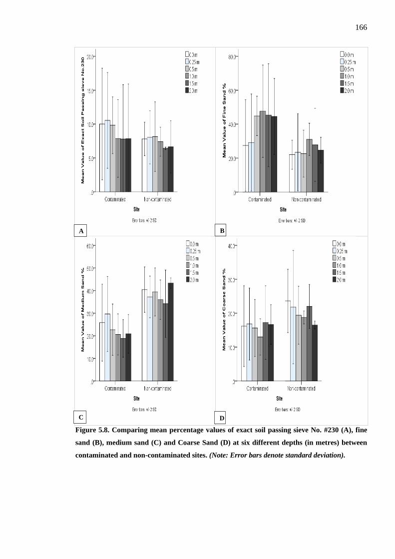
166
Figure 5.8. Comparing mean percentage values of exact soil passing sieve No. #230 (A), fine
sand (B), medium sand (C) and Coarse Sand (D) at six different depths (in metres) between
contaminated and non-contaminated sites. (Note: Error bars denote standard deviation).
A
C
B
D
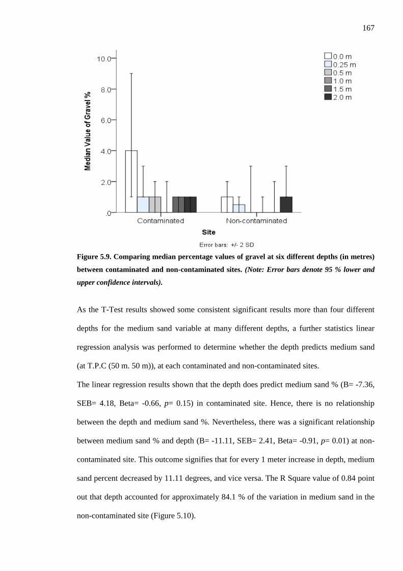
167
Figure 5.9. Comparing median percentage values of gravel at six different depths (in metres)
between contaminated and non-contaminated sites. (Note: Error bars denote 95 % lower and
upper confidence intervals).
As the T-Test results showed some consistent significant results more than four different
depths for the medium sand variable at many different depths, a further statistics linear
regression analysis was performed to determine whether the depth predicts medium sand
(at T.P.C (50 m. 50 m)), at each contaminated and non-contaminated sites.
The linear regression results shown that the depth does predict medium sand % (B= -7.36,
SEB= 4.18, Beta= -0.66, p= 0.15) in contaminated site. Hence, there is no relationship
between the depth and medium sand %. Nevertheless, there was a significant relationship
between medium sand % and depth (B= -11.11, SEB= 2.41, Beta= -0.91, p= 0.01) at non-
contaminated site. This outcome signifies that for every 1 meter increase in depth, medium
sand percent decreased by 11.11 degrees, and vice versa. The R Square value of 0.84 point
out that depth accounted for approximately 84.1 % of the variation in medium sand in the
non-contaminated site (Figure 5.10).
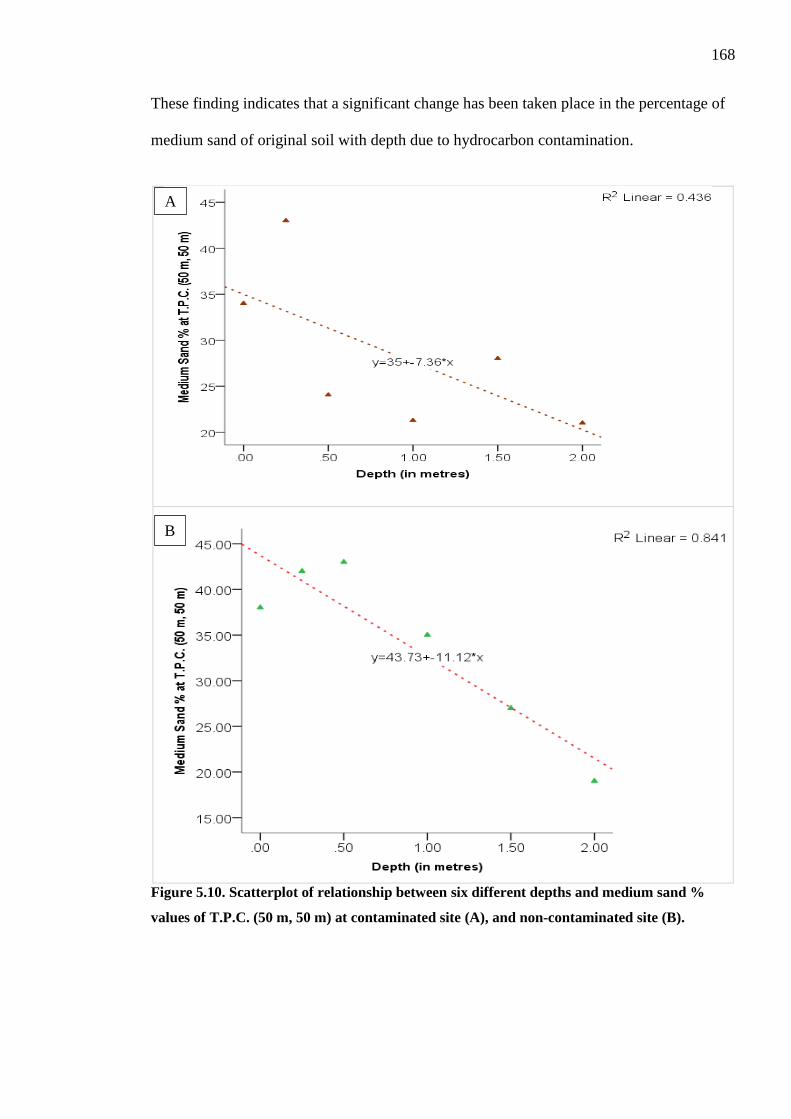
168
These finding indicates that a significant change has been taken place in the percentage of
medium sand of original soil with depth due to hydrocarbon contamination.
Figure 5.10. Scatterplot of relationship between six different depths and medium sand %
values of T.P.C. (50 m, 50 m) at contaminated site (A), and non-contaminated site (B).
A
B

169
Outlier testing was carried out individually for Cu and Cc data and the outlier values were
deleted prior to analysis (Figure 5.11). Following this the normality of the Cu and Cc data
were assessed using the Shapiro-Wilk test of normality. The Cc data at both sites met the
assumption of normality for parametric statistics; however the Cu data violated the
normality assumption, therefore non-parametric statistics were performed on the Cu data
(Tables B.5.17 and B.5.18).
Tables 5.4 and Figures 5.12 & 5.13 below show the significant difference in the median
values of Cu and mean values of Cc in the soil at six different depths between both site
(Table B.5.19). The Mann Whitney U and independent samples T-Test were conducted for
Cu and Cc data, respectively. For Cu data, the Mann Whitney U analysis revealed that
there were significant differences in median values of Cu between contaminated and non-
contaminated sites at only depths 0.0 m (Z= -2.03, U= 4.00 , p= 0.05) and 0.25 m (Z= -
2.15, U= 5.00, p= 0.04). However, this did not achieve significant difference level at other
depths, i.e. 0.5 m, 1.0 m, 1.5 m and 2.0 m. In terms of Cc data, the independent T-Test
analysis revealed that there were significant differences in the mean values of Cc between
the two different sites at depths of 0.0 m (t(21) = -3.93, p= 0.01), 0.25 m (t(25) = -0.82, p=
0.04) and 2.0 m (t(8) = -3.06, p= 0.01). Nevertheless, it did not reach significant difference
level at depths 0.5 m, 1.0 m, 1.5 m and 2.0 m.
The above results (i.e. of Cu and Cc) signify that high contamination leads to a
significantly poorer PSD particularly at the high contamination depth from 0.0 m to 0.5 m.
This phenomenon was generally decreased with depth proving lower contamination at
lower depths.
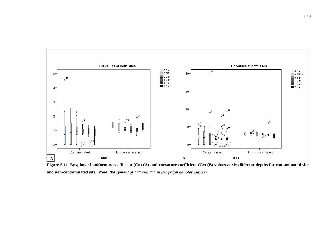
170
Figure 5.11. Boxplots of uniformity coefficient (Cu) (A) and curvature coefficient (Cc) (B) values at six different depths for contaminated site
and non-contaminated site. (Note: the symbol of “*” and “°” in the graph denotes outlier).
A B

171
Table 5.4. The significant differences of the Cu and Cc variables in the soil at six different depths between contaminated and
non-contaminated sites. (Note: outlier vales were deleted in this table).
Depth (m) Variable Site Name N Mean Median SD Min Max Z U t-value p-value
0.0 Cu
Contaminated 22 4.35 3.74 3.23 0.00 11.6 -2.03 4.00 ---- 0.05*
Non-contaminated 5 6.09 6.29 0.84 5.00 7.05
Cc Contaminated 22 0.69 0.69 0.68 0.00 2.33
---- ---- -3.93 0.01* Non-contaminated 5 1.38 1.37 0.22 1.16 1.64
0.25 Cu
Contaminated 22 3.99 4.00 3.60 0.00 10.00 -2.15 5.00 ---- 0.04*
Non-contaminated 5 5.88 6.00 0.51 5.08 6.50
Cc Contaminated 22 0.84 0.78 0.87 0.00 2.57
---- ---- -0.82 0.04* Non-contaminated 5 1.20 0.96 0.40 0.85 1.76
0.5 Cu
Contaminated 22 6.07 4.92 8.83 0.00 40.00 -0.79 11.00 ---- 0.53
Non-contaminated 5 6.00 6.61 1.35 4.25 7.36
Cc Contaminated 22 0.81 0.87 0.55 0.00 2.03
---- ---- -1.61 0.12 Non-contaminated 5 1.14 1.05 0.24 0.94 1.55
1.0 Cu
Contaminated 22 2.74 2.85 1.60 0.00 6.57 -0.18 14.00 ---- 0.93
Non-contaminated 5 5.47 5.79 0.95 3.81 6.12
Cc Contaminated 22 0.77 0.97 0.43 0.00 1.19
---- ---- -1.65 0.13 Non-contaminated 5 1.04 0.99 0.30 0.72 1.40
1.5 Cu
Contaminated 22 3.90 2.80 3.77 0.00 15.71 -0.96 7.50 ---- 0.35
Non-contaminated 5 6.77 5.63 2.93 5.10 12.00
Cc Contaminated 22 0.78 0.90 0.46 0.00 1.31
---- ---- -1.26 0.21 Non-contaminated 5 1.11 1.01 0.46 0.64 1.88
2.0 Cu
Contaminated 22 3.56 3.28 3.86 0.00 18.33 -0.80 13.0 ---- 0.48
Non-contaminated 5 4.81 4.875 1.31 3.28 6.21
Cc Contaminated 22 0.76 0.93 0.45 0.00 1.30
---- ---- -3.06 0.01* Non-contaminated 5 1.32 1.48 0.34 0.89 1.71
*Note: p < .05 indicates to the significant difference in the varibales between two different groups.

172
Figure 5.12. Comparing mean values of uniformity curvature (Cc) in the soil at six different
depths between contaminated and non-contaminated site. (Note: Error bars denote standard
deviation).
Figure 5.13. Comparing median values of uniformity coefficient (Cu) in the soil at six
different depths between contaminated and non-contaminated site. (Note: Errors bars denote
95 % confidence interval).
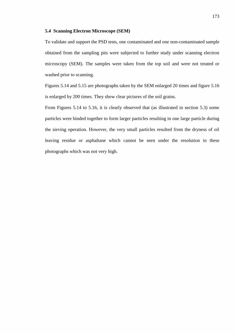
173
5.4 Scanning Electron Microscope (SEM)
To validate and support the PSD tests, one contaminated and one non-contaminated sample
obtained from the sampling pits were subjected to further study under scanning electron
microscopy (SEM). The samples were taken from the top soil and were not treated or
washed prior to scanning.
Figures 5.14 and 5.15 are photographs taken by the SEM enlarged 20 times and figure 5.16
is enlarged by 200 times. They show clear pictures of the soil grains.
From Figures 5.14 to 5.16, it is clearly observed that (as illustrated in section 5.3) some
particles were binded together to form larger particles resulting in one large particle during
the sieving operation. However, the very small particles resulted from the dryness of oil
leaving residue or asphaltane which cannot be seen under the resolution in these
photographs which was not very high.
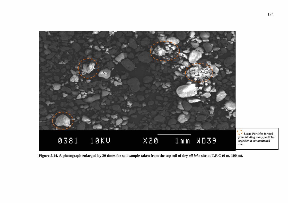
174
Figure 5.14. A photograph enlarged by 20 times for soil sample taken from the top soil of dry oil lake site at T.P.C (0 m, 100 m).
Large Particles formed from binding many particles together at contaminated site.

175
Figure 5.15. A photograph enlarged by 20 times for soil sample taken from the top soil of non-contaminated Site at T.P.C (0 m, 100 m).
Shows no binding material between particles at non-contaminated site.
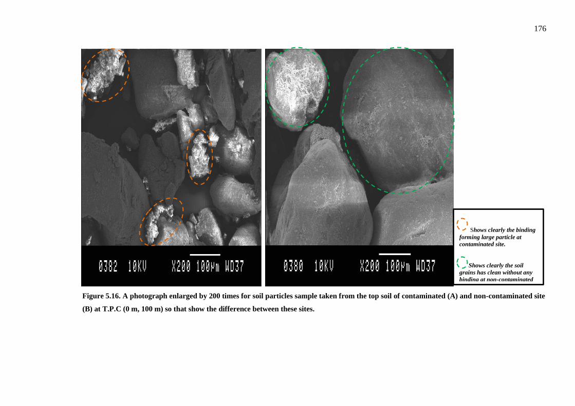
176
Figure 5.16. A photograph enlarged by 200 times for soil particles sample taken from the top soil of contaminated (A) and non-contaminated site
(B) at T.P.C (0 m, 100 m) so that show the difference between these sites.
Shows clearly the binding forming large particle at contaminated site. Shows clearly the soil grains has clean without any binding at non-contaminated site.

177
5.5 Permeability (Hydraulic Conductivity)
5.5.1 Laboratory Results of Permeability
Table B.5.20 illustrates the results of the permeability coefficient of 24 undisturbed soil
samples collected from the contaminated site (dry oil lake); the coefficient of permeability
of the 12 undistributed soil samples obtained from the non-contaminated site are shown in
Table B.5.21. The minimum, maximum, mean and standard deviation values have also
been recorded in the tables for samples taken from each depth.
Table 5.5 shows the mean calculated permeability values against the depth from ground
surface of samples taken from both contaminated and non-contaminated sites. Figure 5.17
represents these mean values against the depth. It should be noted that generally there is no
clear difference between the permeability of the contaminated and non-contaminated soil
and no clear interpretation for the change in permeability with the depth except at a depth
of 0.25 m of the non-contaminated site. This odd change may be attributed to the shortage
in the number of tests made on samples (only two trial pits were chosen from the non-
contaminated site for this test).
Considering Hazen’s Rule of approximation for permeability of soil and according to the
following equation (Cedergren, 1997, p.43):
K= C x (D10)2, Where:
K= Permeability (hydraulic conductivity m/day).
D10= the effective diameter (mm), which can be found from the PSD of soil. i.e. the
diameter of sieve where 10 % of the grains pass through.
C= Constant value range from 1000 to 1500 (unit less).
Hazen’s equation is justified for sands having uniformity coefficients below 5 and an
effective grain size of 0.1 to 3.0 mm. The permeability was calculated based on the above
equation taking an average value of C= 1250.

178
The results are shown in the same figure 5.17. The figure indicates that the calculated
values are in the same order of measured values. However, there was not much difference
between the calculated permeability of contaminated and non-contaminated soil.
Khamehchiyan et al. (2007), investigated the influence of crude oil on the permeability of
clay and sandy soils such SP, SM and CL by mixing them with different amounts of crude
oil; i.e. 2 %, 4 %, 8 %, 12 %, and 16 % by dry weigh. They have suggested that there is an
inverse relationship between permeability and oil content, since there was a decrease in the
coefficient of permeability when the oil content was increased. Rahman et al. (2010) also
showed that hydrocarbon contaminated soil led to a decrease in permeability because oil
clogs some inter-particle spaces. Therefore, any increase in the oil amount will decrease
any available inter-particle spaces for any water leakage. Other studies on similar soil, such
as Al-Sanad et al. (1995) and Al-Sanad and Ismael (1997) have supported the above
findings.
It is important to note that the majority of these studies were conducted with a
comparatively short duration of hydrocarbon contamination prior to testing as compared to
more than two decades of contamination of the soil under Kuwait’s hot climate in the
present study. Furthermore, the interaction of hydrocarbon contamination can change the
particle size distribution in the soil. More uniformly graded soil with gap grading, as in the
present study, would leave more inter-particle voids, allowing higher water permeability
than for a well-graded soil.
In fact, this study has found no clear correlation between hydrocarbon contamination and
permeability of the soil, particularly at the top soil (from around 0.0 m to 0.5 m). However,
at deeper depths, (as expected) and as shown in figure 5.17, the permeability for both sites
becomes closer which infers a lower contamination, at deep depths, of the contaminated
site.
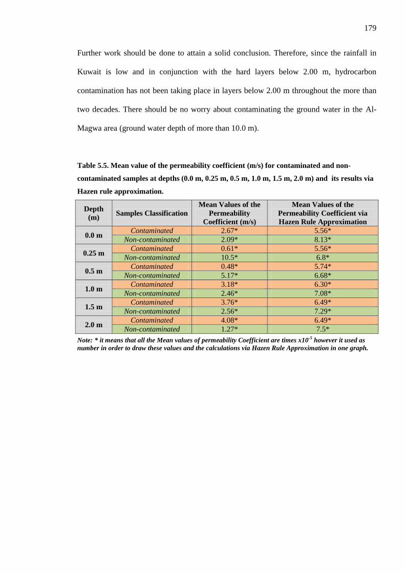
179
Further work should be done to attain a solid conclusion. Therefore, since the rainfall in
Kuwait is low and in conjunction with the hard layers below 2.00 m, hydrocarbon
contamination has not been taking place in layers below 2.00 m throughout the more than
two decades. There should be no worry about contaminating the ground water in the Al-
Magwa area (ground water depth of more than 10.0 m).
Table 5.5. Mean value of the permeability coefficient (m/s) for contaminated and non-
contaminated samples at depths (0.0 m, 0.25 m, 0.5 m, 1.0 m, 1.5 m, 2.0 m) and its results via
Hazen rule approximation.
Depth (m) Samples Classification
Mean Values of the Permeability
Coefficient (m/s)
Mean Values of the Permeability Coefficient via Hazen Rule Approximation
0.0 m Contaminated 2.67* 5.56*
Non-contaminated 2.09* 8.13*
0.25 m Contaminated 0.61* 5.56*
Non-contaminated 10.5* 6.8*
0.5 m Contaminated 0.48* 5.74*
Non-contaminated 5.17* 6.68*
1.0 m Contaminated 3.18* 6.30*
Non-contaminated 2.46* 7.08*
1.5 m Contaminated 3.76* 6.49*
Non-contaminated 2.56* 7.29*
2.0 m Contaminated 4.08* 6.49*
Non-contaminated 1.27* 7.5*
Note: * it means that all the Mean values of permeability Coefficient are times x10-5 however it used as number in order to draw these values and the calculations via Hazen Rule Approximation in one graph.
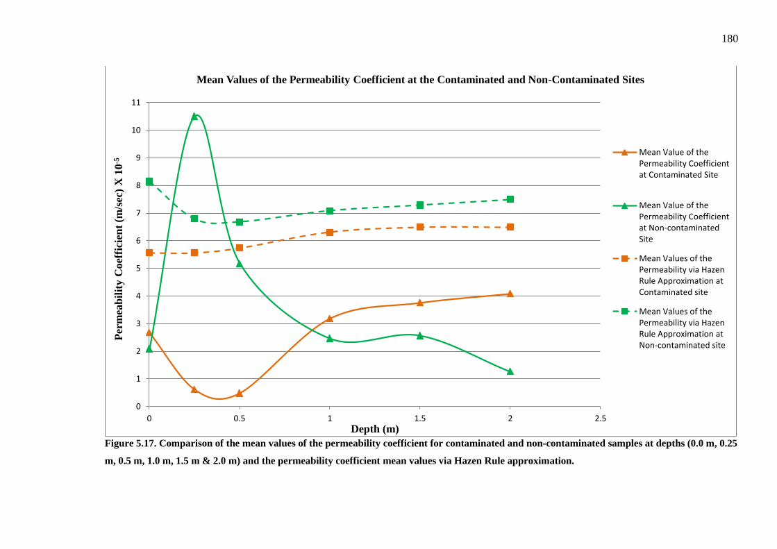
180
Figure 5.17. Comparison of the mean values of the permeability coefficient for contaminated and non-contaminated samples at depths (0.0 m, 0.25
m, 0.5 m, 1.0 m, 1.5 m & 2.0 m) and the permeability coefficient mean values via Hazen Rule approximation.
0
1
2
3
4
5
6
7
8
9
10
11
0 0.5 1 1.5 2 2.5
Per
mea
bilit
y C
oeff
icie
nt (m
/sec
) X
10-5
Depth (m)
Mean Values of the Permeability Coefficient at the Contaminated and Non-Contaminated Sites
Mean Value of thePermeability Coefficientat Contaminated Site
Mean Value of thePermeability Coefficientat Non-contaminatedSite
Mean Values of thePermeability via HazenRule Approximation atContaminated site
Mean Values of thePermeability via HazenRule Approximation atNon-contaminated site
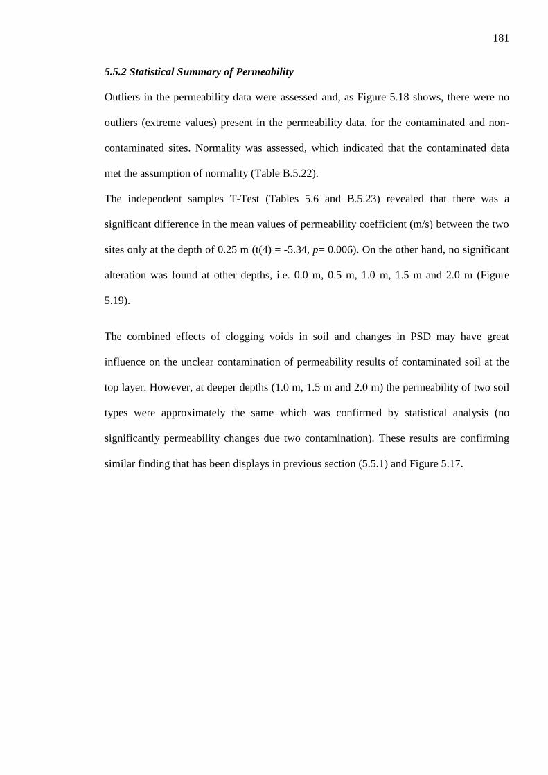
181
5.5.2 Statistical Summary of Permeability Outliers in the permeability data were assessed and, as Figure 5.18 shows, there were no
outliers (extreme values) present in the permeability data, for the contaminated and non-
contaminated sites. Normality was assessed, which indicated that the contaminated data
met the assumption of normality (Table B.5.22).
The independent samples T-Test (Tables 5.6 and B.5.23) revealed that there was a
significant difference in the mean values of permeability coefficient (m/s) between the two
sites only at the depth of 0.25 m (t(4) = -5.34, p= 0.006). On the other hand, no significant
alteration was found at other depths, i.e. 0.0 m, 0.5 m, 1.0 m, 1.5 m and 2.0 m (Figure
5.19).
The combined effects of clogging voids in soil and changes in PSD may have great
influence on the unclear contamination of permeability results of contaminated soil at the
top layer. However, at deeper depths (1.0 m, 1.5 m and 2.0 m) the permeability of two soil
types were approximately the same which was confirmed by statistical analysis (no
significantly permeability changes due two contamination). These results are confirming
similar finding that has been displays in previous section (5.5.1) and Figure 5.17.

182
Figure 5.18. Boxplots of permeability coefficient (m/s) values in the soil at six different depths
for contaminated site and non-contaminated site.
Table 5.6. The significant differences of the permeability coefficient (m/s) variable in the soil
at six different depths between contaminated and non-contaminated sites.
Depth
(m) Site Name N Mean SD Min Max t-value p-value
0.0 Contaminated 4 2.68x10⁻⁵ 1.44 x 10⁻⁵ 2.0 x 10⁻⁵ 5.0 x 10⁻⁵
0.48 0.67 Non-contaminated 2 2.10 x 10⁻⁵ 1.35x10⁻⁵ 1.0 x 10⁻⁵ 3.0 x 10⁻⁵
0.25 Contaminated 4 6.0x10⁻⁶ 8.3x10⁻⁶ 0 1.78 x 10⁻⁵
-5.34 0.006* Non-contaminated 2 1.0 x10⁻⁴ 4.03x10⁻⁵ 7.69x10⁻⁵ 1.34x10⁻⁴
0.5 Contaminated 4 4.81x10⁻⁶ 5.6x10⁻⁶ 0 1.07x10⁻⁵
-1.17 0.44 Non-contaminated 2 5.1x10⁻⁵ 6.2x10⁻⁵ 7.6x10⁻⁶ 9.5x10⁻⁵
1.0 Contaminated 4 3.1x10⁻⁵ 1.06x10⁻⁵ 2.19x10⁻⁵ 4.64x10⁻⁵
0.29 0.81 Non-contaminated 2 2.4 x10⁻⁵ 3.3x10⁻⁵ 1.0x10⁻⁶ 4.82x10⁻⁵
1.5 Contaminated 4 3.76x10⁻⁵ 1.4x10⁻⁵ 1.72x10⁻⁵ 4.93x10⁻⁵
1.02 0.40 Non-contaminated 2 2.56x10⁻⁵ 1.3x10⁻⁵ 1.63x10⁻⁵ 3.49x10⁻⁵
2.0 Contaminated 4 4.0x10⁻⁵ 1.29x10⁻⁵ 2.67x10⁻⁵ 5.81x10⁻⁵
2.47 0.06 Non-contaminated 2 1.27x10⁻⁵ 1.35x10⁻⁵ 3.1x10⁻⁶ 2.23x10⁻⁵
*Note, p < .05 indicates to the significant difference in the variable between two different groups.

183
Figure 5.19. Comparing mean values of permeability coefficient (m/s) in the soil at six
different depths between contaminated and non-contaminated site. (Note: Error bars denote
standard deviation).

184
5.6 Shear Strength 5.6.1 Laboratory Results of Shear Strength
Table (B.5.24) shows the results of Direct Shear strength tests on contaminated samples
with hydrocarbon at different depths; the shear strength test of samples collected from
control sites are shown in Table (B.5.25). The cohesion parameters (c) were zero for all the
soil samples for both sites indicating that this level of hydrocarbon contamination does not
generate cohesion in such types of soil. Therefore, only the angles of friction parameters
(φ) were listed in the tables. The minimum, maximum, mean and standard deviation values
of angle of friction parameter (φ) for samples taken from each depth were recorded in the
tables. For more details, some typical shear behaviour curves (showing strain under
different shear and normal stresses) are shown in figures B.5.3 to B.5.62.
Table 5.7 and figure 5.20 show the mean values of strength parameter (φ) of both
contaminated and non-contaminated sites. The angle of internal friction is shown to be
steadily and clearly decreased due to hydrocarbon contamination in all samples. However,
the decrease due to hydrocarbon contamination was generally lowered with depths which
may be consistently related to the lower soil contamination with hydrocarbon at the deeper
depths.
In an experimental study by Singh et al. (2009), soil was mixed with different percentages
of used motor oil and subjected to a shear test. The results showed that the effective angle
of internal friction for poorly graded sand decreases significantly. On mixing with 9 %, the
angle of friction decreased from 36.58 in the virgin state to 24.58. Shin et al. (1999)
reported a reduction in the shear strength of sandy soil between 23 % and 27 % due to 1.3
% oil addition. The reduction was attributed to the oil coating soil grain surfaces resulting
in the slipping of soil grains over each other. Al-Sanad et al. (1995) also conducted a test
in Kuwait (Jahra Sand) by mixing it in the lab with crude oil of 2 %, 4 % and 6 %.

185
In agreement with the studies shown above, they showed a reduction in shear strength
with an associated increase in the oil content; this reduction depended on the viscosity of
the oil. However, reduction in shear strength of non-cohesive soil of the above study
cannot be compared with the current study because, in the current study, the oil was dry
and an increase in the viscosity between particles was not expected. In fact, it actually
binds some particles leading to higher uniformity in PSD as discussed in section 5.3. The
higher uniformity in PSD may thus be responsible for the lower strength in the
contaminated soil of the current study.
Table 5.7. Comparing the mean values of the angle of internal friction (φ) for contaminated
and non-contaminated soil samples at six different depths of 0.0 m, 0.25 m, 0.5 m, 1.0 m, 1.5
m and 2.0 m.
Depth Samples Classification
Mean Value of the Strength Parameters Angle of Internal Friction
(φ)
0.0 m Contaminated 30.8 Non-Contaminated 37.16
0.25 m Contaminated 32 Non-Contaminated 36
0.5 m Contaminated 32.8 Non-Contaminated 39.3
1.0 m Contaminated 33 Non-Contaminated 37.9
1.5 m Contaminated 33 Non-Contaminated 37.13
2.0 m Contaminated 33.6 Non-Contaminated 36.63

186
Figure 5.20. Comparing the mean values of the angle of internal friction (φ) for contaminated (brown colour) and non-contaminated (green
colour) soil samples at six different depths of 0.0 m, 0.25 m, 0.5 m, 1.0 m, 1.5 m & 2.0 m.
20
25
30
35
40
45
0 0.25 0.5 0.75 1 1.25 1.5 1.75 2 2.25
An
gle
of
Inte
rnal
fri
ctio
n (φ)
Depth (m)
Mean Value of the Angle of Internal Friction (φ) at Contaminated & Non-contaminated Site
Mean Value of the Angle of Internal Friction (φ) at contaminated site
Mean Value of the Angle of Internal Friction (φ) at Uncontaminated site

187
5.6.2 Statistical Summary of Shear Strength Figure 5.21 shows no outliers present in the angle of internal friction data. The assumption
of normality was also largely met as ten of the twelve Shapiro-Wilk p-values were above
0.05. Therefore, parametric statistics were appropriate for the analyses. (Table B.5.26).
An independent samples T-Test found a significant difference in mean angle of internal
friction (φ) values between contaminated and non-contaminated sites (Table 5.8 and
B.5.27). Consistent across the six different depths, mean values were lower in the
contaminated site than the non-contaminated site. The analysis revealed that there were
significant differences in the mean values of angle of internal friction (φ) between both
sites at depths 0.0 m (t(8) = -6.46, p= 0.01), 0.25 m (t(8) = -3.25, p= 0.01), 0.5 m (t (8) = -
9.07, p= 0.001), 1.0 m (t (8) = -4.46, p= 0.02), 1.5 m (t (8) = -4.52, p= 0.01) and 2.0 m (t
(8) = -3.08, p= 0.01) (Figure 5.22).
These results confirm those illustrated in section (5.6.1), i.e. that hydrocarbon
contamination reduces strength.

188
Figure 5.21. Boxplots of angle of internal friction (φ) values in the soil at six different depths
for contaminated site and non-contaminated site.
Table 5.8. The significant differences of the angle of internal friction (φ) variable in the soil at
six different depths between contaminated and non-contaminated sites.
Depth (m) Site Name N Mean SD Min Max t-value p-value
0.0 Contaminated 7 30.85 2.54 28 35
-6.46
0.001* Non-contaminated 3 37.16 .28 37 37.5
0.25 Contaminated 7 32.42 1.51 30 34
-3.25
0.012* Non-contaminated 3 36.00 1.80 34 37.5
0.5 Contaminated 7 32.85 1.06 31 34
-9.07
0.001* Non-contaminated 3 39.30 .90 38.4 40.2
1.0 Contaminated 7 33.00 1.15 31 34
-4.46
0.002* Non-contaminated 3 37.90 2.47 36 40.7
1.5 Contaminated 7 33.00 1.29 31 34
-4.52
0.002* Non-contaminated 3 37.13 1.41 35.5 38
2.0 Contaminated 7 33.57 .97 32 35
-3.08
0.015* Non-contaminated 3 36.63 2.32 34 38.4
*Note, p < 0.05 indicates to the significant difference in the variable between two different groups.

189
Figure 5.22. Comparing mean values of the angle of internal friction (φ) in the soil at six
different depths between contaminated and non-contaminated site. (Note: Error bars denote
standard deviation).
As the T-Test results and figure 5.22 (above) showed significantly different results for the
mean values of angle of internal friction at six different depths between the two sites, a
further statistical linear regression analysis was conducted to determine whether the depth
predicts angle of internal friction (φ) at T.P.C (50 m, 50 m), at each of the contaminated
and non-contaminated sites.
The analysis of the contaminated site found a significant, positive relationship between the
six different depth categories and the angle of internal friction (φ) values (B= 2.69, SEB=
0.84, Beta= 0.84, p= 0.03). The R Square value of 0.719 indicates that depth categories
accounted for approximately 71.9 % of the angle of internal friction (φ) values. For every 1
meter increase in depth, the angle of internal friction increased by 2.69 degrees. On the
other hand, the analysis found that there was no significant relationship between depth

190
categories and the angle of internal friction values at the non-contaminated site (B= 0.01,
SEB= 0.85, Beta= 0.007, p= 0.98). The R Square value of 0.000 indicates that the depth
categories accounted for none (0 %) of the angle of internal friction values (Figure 5.23).
191
Figure 5.23. Scatterplot showing relationship between six different depth categories and angle of internal friction (φ) at T.P.C (50 m, 50 m), at
contaminated site (A) and non-contaminated site (B).
A B

192
5.7 Summary
This Chapter has presented the findings of the geotechnical characteristics of soil samples
taken from two different locations, i.e. the contaminated (dry oil lake) and non-
contaminated sites. All the findings of the geotechnical characterisation of soil were
subjected to a statistical analysis in order to support and provide a solid conclusion. The
investigated properties were plasticity, PSD, SEM, permeability coefficient (hydraulic
conductivity) and shear strength. The following conclusions were drawn from this analysis:
None of the samples showed any plastic behavior so the soil is considered to be
non- plastic (in both contaminated and non-contaminated sites).
Wide ranges were found in the gradation of soil samples taken from the same depth
but from different T.P.C locations at the contaminated site, particularly in the top
soil; however, it becomes narrower at lower depths. This was expected because the
hydrocarbon contamination content differs from point to point in the top soil. In the
non-contaminated site, it was noted that (at one depth), the gradation range between
a sample taken from one T.P.C and another was smaller than in the corresponding
contaminated site. The small particles (passing No.#230) and large (gravel %)
percentage values of the soil classification for the samples taken from the
contaminated site were slightly higher than those for samples taken from the non-
contaminated site, especially from the top soil where hydrocarbon contamination
was found to be higher. The statistical analysis proved that there were significant
differences in the percentage values of soil classification constituents with only
medium sand, coarse sand, gravel and exact soil (passing sieve No.#230) between
both sites at a depth of 0.0 m. Additionally, a significant differences were found at
both sites for the percentage values of fine sand (at depths 0.5 m, 1.0 m and 2.0 m)

193
medium sand (at depths 0.25 m, 0.5 m, 1.0 m, 1.5 m and 2.0 m), coarse sand (at
depths 1.0 m and 1.5 m) and gravel (at depth 0.25 m).
In terms of the results of the Coefficient of Permeability no clear difference was
found between the contaminated and non-contaminated soil and no clear change
was found in the permeability with the depth except at depth 0.25 m for the non-
contaminated site. A statistical analysis also confirms that there was significant
difference in the mean value of permeability coefficient between the two sites at
only 0.25 m depth.
The angle of internal friction decreased due to hydrocarbon contamination in all
samples. Although, this decrease was lower at deeper depths. The statistical finding
ascertained that there were significant differences in the mean values of the angle
of internal friction between the two sites at all six different depths of 0.0 m, 0.25 m,
0.5 m, 1.0 m, 1.5 m and 2.0 m. Furthermore, it found statistically that the angle of
internal friction (φ) values increased with an increase in the depth at the
contaminated site; however, it found no relationship between the angle of internal
friction (φ) values and depth at the non-contaminated site.
The next chapter will investigate the changes in geochemical characteristics of soil due to
hydrocarbon contamination through comparing the geochemical properties of the soil
samples extracted from both contaminated and non-contaminated sites.
194
6. GEOCHEMICAL CHARACTERISATION
6.1 Introduction
This chapter presents the results of changes in geochemical characteristics of soil due to
hydrocarbon contamination of two decades at the Greater Burgan Oil Field region (Al-
Magwa area-dry oil lake site). Results were achieved by comparing the findings of the
soil’s geochemical properties extracted from both the contaminated and non-contaminated
sites. These results will be discussed to demonstrate how the study aims can be achieved
by correlating the findings of the experiment with the studies found in the literature. The
results of the geochemical characteristics of the soil samples will also be statistically
analysed in this chapter so as to support any solid findings. The results of geochemical
characterisations include: pH; water soluble Cl- and (SO3 & SO4); (EA); and GC-MS.
Some of the test findings are presented in this chapter in the form of limited typical tables
and figures, however, most of the tables and figures can be seen in appendix C.
6.2 Hydrogen Ion Concentration (pH)
6.2.1 Laboratory Results of pH
Table 6.1 displays the pH results of contaminated soil samples taken from the dry oil lake
while the corresponding results for the non-contaminated soil samples are shown in Table
6.2. The maximum and minimum values are also shown in these tables.
Table 6.1 shows that there is a wide range between the maximum and minimum pH values
of samples taken from different T.P.C. at the same depth for the hydrocarbon contaminated
site as compared with the corresponding values of the non-contaminated site (Table 6.2).
Table 6.3 and figure 6.1 further emphasises the range between maximum and minimum
values at different depths. This wide range from the hydrocarbon contaminated site was
expected and was the justification for taking more numerous testing samples from this site
195
than those from the non-contaminated site. This was a common factor in testing greater
sample numbers (for all testings in this study) from the hydrocarbon contaminated sites.
Furthermore, the table and figure show that there is a considerable decrease in the
minimum values of pH due to contamination which means that contamination increased
the acidity of soil which increases the difficulty for growing plants.
From Table 6.3, it can be seen that the lowest value of the pH for the contaminated soil
was 7.02 through all depths which, according to the classification of Horneck et al. (2011),
is within the limiting range of neutral soil (6.6 - 7.3) (Table 3.4). The contaminated soil is
therefore considered to be still available for agricultural activities although contamination
lowers its validation.
Table 6.3 shows that the pH values in the contaminated area ranges from (7.02 to 9.37).
Other studies, including those of Al-Duwaisan and Al-Naseem (2011, p.441) found that the
pH values range from 7.59 to 8.1. Their research was also carried out in the Burgan area.
Barua et al. (2011), Khuraibet and Attar (1995) and Rahman et al. (2007) reported an
increase in acidity of hydrocarbon contamination due to the formation of toxic acids in the
spilled oil. Furthermore, a study by Barua et al. (2011) indicated that crude oil
contaminated soil is slightly more acidic in nature which may be due to the formation of
toxic acids in the spilled oils.
A study of five different oil polluted sites by Khuraibet and Attar (1995) concluded that the
soil was generally neutral in pH, becoming slightly more alkaline with depth, suggesting
that the presence of oil may lower soil pH which could have a detrimental effect on plant
growth. Additionally, Habib-ur-Rahman et al. (2007), investigated the pH of soil
contaminated with crude oil; they found that the pH values of non-contaminated and
contaminated soil were 7.605 and 7.511 respectively. They also indicated that there was a
slight reduction of pH for crude oil contaminated clays, showing the acidic nature of the
crude oil.
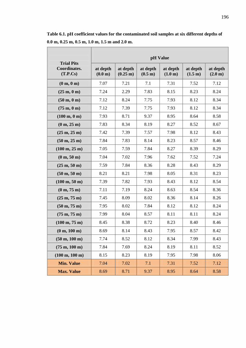
196
Table 6.1. pH coefficient values for the contaminated soil samples at six different depths of
0.0 m, 0.25 m, 0.5 m, 1.0 m, 1.5 m and 2.0 m.
Trial Pits Coordinates.
(T.P.Cs)
pH Value
at depth (0.0 m)
at depth (0.25 m)
at depth (0.5 m)
at depth (1.0 m)
at depth (1.5 m)
at depth (2.0 m)
(0 m, 0 m) 7.07 7.21 7.1 7.31 7.52 7.12
(25 m, 0 m) 7.24 2.29 7.83 8.15 8.23 8.24
(50 m, 0 m) 7.12 8.24 7.75 7.93 8.12 8.34
(75 m, 0 m) 7.12 7.39 7.75 7.93 8.12 8.34
(100 m, 0 m) 7.93 8.71 9.37 8.95 8.64 8.58
(0 m, 25 m) 7.83 8.34 8.19 8.27 8.52 8.67
(25 m, 25 m) 7.42 7.39 7.57 7.98 8.12 8.43
(50 m, 25 m) 7.84 7.83 8.14 8.23 8.57 8.46
(100 m, 25 m) 7.05 7.59 7.84 8.27 8.39 8.29
(0 m, 50 m) 7.04 7.02 7.96 7.62 7.52 7.24
(25 m, 50 m) 7.59 7.84 8.36 8.28 8.43 8.29
(50 m, 50 m) 8.21 8.21 7.98 8.05 8.31 8.23
(100 m, 50 m) 7.39 7.82 7.93 8.43 8.12 8.54
(0 m, 75 m) 7.11 7.19 8.24 8.63 8.54 8.36
(25 m, 75 m) 7.45 8.09 8.02 8.36 8.14 8.26
(50 m, 75 m) 7.95 8.02 7.84 8.12 8.12 8.24
(75 m, 75 m) 7.99 8.04 8.57 8.11 8.11 8.24
(100 m, 75 m) 8.45 8.38 8.72 8.23 8.40 8.46
(0 m, 100 m) 8.69 8.14 8.43 7.95 8.57 8.42
(50 m, 100 m) 7.74 8.52 8.12 8.34 7.99 8.43
(75 m, 100 m) 7.84 7.69 8.24 8.19 8.11 8.52
(100 m, 100 m) 8.15 8.23 8.19 7.95 7.98 8.06
Min. Value 7.04 7.02 7.1 7.31 7.52 7.12
Max. Value 8.69 8.71 9.37 8.95 8.64 8.58

197
Table 6.2. pH coefficient values for the non-contaminated soil samples at six different depths
of 0.0 m, 0.25 m, 0.5 m, 1.0 m, 1.5 m and 2.0 m.
Trial Pits Coordinates. (T.P.Cs)
pH Value
at depth (0.0 m)
at depth (0.25 m)
at depth (0.5 m)
at depth (1.0 m)
at depth (1.5 m)
at depth (2.0 m)
(0 m, 0 m) 7.93 7.85 8.23 8.06 8.15 8.24
(100 m, 0 m) 7.59 8.02 8.12 8.19 8.24 8.26
(50 m, 50 m) 8.12 8.04 8.19 8.24 8.27 8.24
(0 m, 100 m) 8.12 8.15 8.27 8.39 8.31 8.36
(100 m, 100 m) 7.84 7.93 8.11 8.04 8.12 8.06
Min. Value 7.59 7.85 8.11 8.04 8.12 8.06
Max. Value 8.12 8.15 8.27 8.39 8.31 8.36
Table 6.3. Minimum, maximum and range of pH values in the soil at six different
depths for contaminated and non-contaminated sites.
Depth (m) Samples Classification
pH Minimum Value
pH Maximum Value pH Range Value
0.0 m Contaminated 7.04 8.69 1.65
Non-contaminated 7.59 8.12 0.53
0.25 m Contaminated 7.02 8.71 1.69
Non-contaminated 7.85 8.15 0.3
0.5 m Contaminated 7.1 9.37 2.27
Non-contaminated 8.11 8.27 0.16
1.0 m Contaminated 7.31 8.95 1.64
Non-contaminated 8.04 8.39 0.35
1.5 m Contaminated 7.52 8.64 1.12
Non-contaminated 8.12 8.31 0.19
2.0 m Contaminated 7.12 8.58 1.55
Non-contaminated 8.06 8.36 0.3
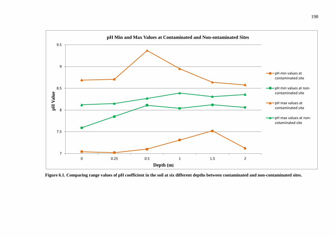
198
Figure 6.1. Comparing range values of pH coefficient in the soil at six different depths between contaminated and non-contaminated sites.
7
7.5
8
8.5
9
9.5
0 0.25 0.5 1 1.5 2
pH V
alue
Depth (m)
pH Min and Max Values at Contaminated and Non-ontaminated Sites
pH min values atcontaminated site
pH min values at non-contaminated site
pH max values atcontaminated site
pH max values at non-cotaminated site
199
6.2.2 Statistical Summary of pH
Figure 6.2 displays outliers in contaminated and non-contaminated pH data, which were
deleted from the dataset. Table 6.5 and figure 6.3 show minimum and maximum values of
pH coefficient in the soil samples at six different depths between contaminated and non-
contaminated sites.
The table and figure show that there is a significant increase in the maximum and
minimum pH values of contaminated soil at all depths, particularly at the top layer,
indicating that the range between maximum and minimum pH values increased due to
contamination. This increase in the range was more obvious at the top layer, (it generally
decreases at deeper depths).
Comparing the results in Tables (6.3 and 6.4) show that the minimum value of pH did not
change and so it cannot be stated that the statistical analysis displays a difference in the
availability of soil for agricultural activities.
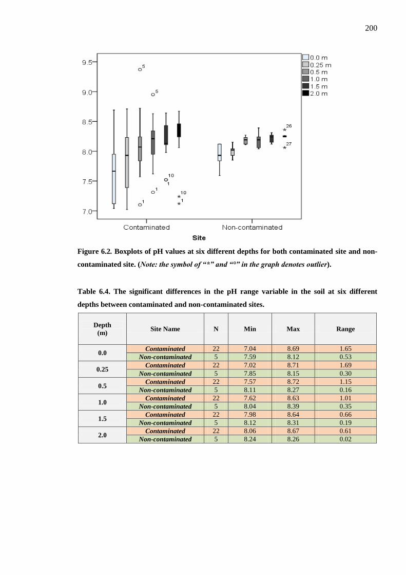
200
Figure 6.2. Boxplots of pH values at six different depths for both contaminated site and non-
contaminated site. (Note: the symbol of “*” and “°” in the graph denotes outlier).
Table 6.4. The significant differences in the pH range variable in the soil at six different
depths between contaminated and non-contaminated sites.
Depth (m)
Site Name N Min Max Range
0.0 Contaminated 22 7.04 8.69 1.65
Non-contaminated 5 7.59 8.12 0.53
0.25 Contaminated 22 7.02 8.71 1.69
Non-contaminated 5 7.85 8.15 0.30
0.5 Contaminated 22 7.57 8.72 1.15
Non-contaminated 5 8.11 8.27 0.16
1.0 Contaminated 22 7.62 8.63 1.01
Non-contaminated 5 8.04 8.39 0.35
1.5 Contaminated 22 7.98 8.64 0.66
Non-contaminated 5 8.12 8.31 0.19
2.0 Contaminated 22 8.06 8.67 0.61
Non-contaminated 5 8.24 8.26 0.02
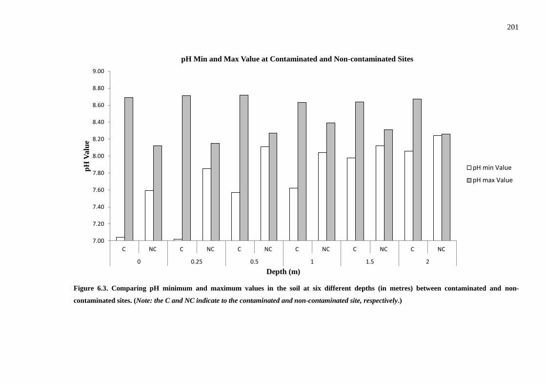
201
Figure 6.3. Comparing pH minimum and maximum values in the soil at six different depths (in metres) between contaminated and non-
contaminated sites. (Note: the C and NC indicate to the contaminated and non-contaminated site, respectively.)
7.00
7.20
7.40
7.60
7.80
8.00
8.20
8.40
8.60
8.80
9.00
C NC C NC C NC C NC C NC C NC
0 0.25 0.5 1 1.5 2
pH V
alue
Depth (m)
pH Min and Max Value at Contaminated and Non-contaminated Sites
pH min Value
pH max Value

202
6.3 Water Soluble Chloride (Cl-) and Sulphate (SO3 & SO4) Content
6.3.1 Laboratory Results of Cl-, SO3 and SO4 Content
The results of the Cl-, SO3 and SO4 tests conducted on contaminated soil samples with
hydrocarbon at various depths are displayed in Tables C.6.1, C.6.2, C.6.3, C.6.4, C.6.5 and
C.6.6; Table C.6.7 shows the results of similar tests on non-contaminated samples. The
maximum, minimum, standard deviation and mean values of these samples at each depth
are documented in the tables.
Table (6.5) and figures from 6.4 to 6.6 show the mean values of water soluble chloride and
sulphates at different soil depths for the contaminated and non-contaminated sites.
As is obvious from tables 6.5 and figure 6.4, the Cl- concentration was very high
(approximately 13000 mg/kg) at the top layer of the hydrocarbon contaminated site. The
concentration was then decreased to less than 4000 mg/kg at depths lower than 0.5 m.
However, at the non-contaminated site, the Cl- concentration was approximately zero.
As noted from Table 6.5 and figures 6.5 and 6.6, for both SO3 and SO4, concentrations at
the top soil layer of the hydrocarbon contaminated site were considerably higher than those
in the non-contaminated site. However, both SO3 & SO4 dropped down suddenly and
considerably at depth to become lower than that in the non-contaminated site at depths
lower than 0.25 m.
The concentration was then further decreased (at the hydrocarbon contaminated site) at
lower depths until it reached an approximately constant value of between 1.0 m and 2.0 m
depths. In the non-contaminated site the concentration of both SO3 & SO4 were
approximately constant throughout the depths.
The Cl- values obtained in this study were in line with the study conducted by Onojake and
Osuji (2012). They also investigated the Cl- and SO3 & SO4 content for soil contaminated
with crude oil after six months of the spill incident and compared it with the control site.
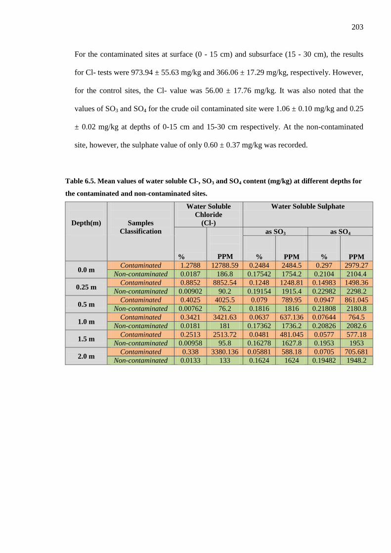
203
For the contaminated sites at surface (0 - 15 cm) and subsurface (15 - 30 cm), the results
for Cl- tests were 973.94 ± 55.63 mg/kg and 366.06 ± 17.29 mg/kg, respectively. However,
for the control sites, the Cl- value was 56.00 ± 17.76 mg/kg. It was also noted that the
values of SO3 and SO4 for the crude oil contaminated site were 1.06 ± 0.10 mg/kg and 0.25
± 0.02 mg/kg at depths of 0-15 cm and 15-30 cm respectively. At the non-contaminated
site, however, the sulphate value of only 0.60 ± 0.37 mg/kg was recorded.
Table 6.5. Mean values of water soluble Cl-, SO3 and SO4 content (mg/kg) at different depths for
the contaminated and non-contaminated sites.
Depth(m)
Samples Classification
Water Soluble Chloride
(Cl-)
Water Soluble Sulphate
%
PPM
as SO3 as SO4
%
PPM
%
PPM
0.0 m Contaminated 1.2788 12788.59 0.2484 2484.5 0.297 2979.27
Non-contaminated 0.0187 186.8 0.17542 1754.2 0.2104 2104.4
0.25 m Contaminated 0.8852 8852.54 0.1248 1248.81 0.14983 1498.36
Non-contaminated 0.00902 90.2 0.19154 1915.4 0.22982 2298.2
0.5 m Contaminated 0.4025 4025.5 0.079 789.95 0.0947 861.045
Non-contaminated 0.00762 76.2 0.1816 1816 0.21808 2180.8
1.0 m Contaminated 0.3421 3421.63 0.0637 637.136 0.07644 764.5
Non-contaminated 0.0181 181 0.17362 1736.2 0.20826 2082.6
1.5 m Contaminated 0.2513 2513.72 0.0481 481.045 0.0577 577.18
Non-contaminated 0.00958 95.8 0.16278 1627.8 0.1953 1953
2.0 m Contaminated 0.338 3380.136 0.05881 588.18 0.0705 705.681
Non-contaminated 0.0133 133 0.1624 1624 0.19482 1948.2
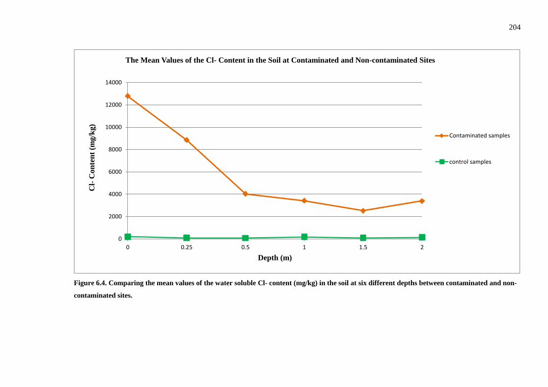
204
Figure 6.4. Comparing the mean values of the water soluble Cl- content (mg/kg) in the soil at six different depths between contaminated and non-
contaminated sites.
0
2000
4000
6000
8000
10000
12000
14000
0 0.25 0.5 1 1.5 2
Cl-
Con
tent
(m
g/kg
)
Depth (m)
The Mean Values of the Cl- Content in the Soil at Contaminated and Non-contaminated Sites
Contaminated samples
control samples

205
Figure 6.5. Comparing the mean values of the water soluble SO3 content (mg/kg) in the soil at six different depths between contaminated and non-
contaminated sites.
0
500
1000
1500
2000
2500
3000
0 0.25 0.5 1 1.5 2
SO3
Con
tent
(m
g/kg
)
Depth (m)
The Mean Values of the SO3 in the Soil at Contaminated and Non-Contaminated Sites
contaminated samples
Control samples

206
Figure 6.6. Comparing the mean values of the water soluble SO4 content (mg/kg) in the soil at six different depths between contaminated and non-
contaminated sites.
0
500
1000
1500
2000
2500
3000
3500
0 0.25 0.5 1 1.5 2
SO4
Con
tent
(m
g/kg
)
Depth (m)
The Mean Values of the SO4 Content in the Soil at Contaminated and Non- Contaminated Sites
contaminated samples
control samples

207
6.3.2 Statistical Summary of Cl-, SO3 and SO4 Content
Figure 6.7 shows the outliers present in the Cl-, SO3 and SO4 data. These outliers were
deleted from the dataset. Data were normally distributed for SO3 and SO4, but the
assumption of normality was violated for CI- data at both sites (Tables C.6.8 and C.6.9).
Table 6.6 shows the median and mean differences between Cl-, SO3 and SO4 values at both
sites.
A non-parametric, Mann Whitney U test found significant differences in the median
concentration values of Cl- (mg/kg) between the two sites at all six depths: 0.0 m depth
(Z= -3.28, U= 2, p= 0.001), 0.25 m depth (Z= -2.95, U= 6, p= 0.01), 0.5 m depth (Z= -
2.95, U= 6, p= 0.001), 1.0 m depth (Z= -3.05, U= 5, p= 0.001), 1.5 m depth (Z= -3.26, U=
2, p= 0.001) and 2.0 m depth (Z= -2.98, U= 2, p= 0.001) (Figure 6.8 and Table C.6.10).
An independent samples T-Test found significant differences in the mean concentration
values of SO3 and SO4 (mg/kg) between contaminated and non-contaminated sites at all six
depths. For SO3, the results revealed that there are significant difference at depths 0.0 m
(t(15) = 1.92, p= 0.005), 0.25 m (t(24) = -2.38, p= 0.02), 0.5 m (t(25) = -2.90, p= 0.008),
1.0 m (t(24) = -4.80, p= 0.001), 1.5 m (t(23) = -7.01, p= 0.001) and 2.0 m (t(25) = -4.19,
p= 0.001). Also, mean values of the SO4 showed significant variance at 0.0 m (t(15) = 1.91,
p= 0.04), 0.25 m (t(14) = -2.49, p= 0.02), 0.5 m (t(25) = -3.20, p= 0.004), 1.0 m (t(12) = -
5.60, p= 0.001), 1.5 m (t(25) = -4.70, p= 0.001) and 2.0 m (t(25) = -4.19, p= 0.001)
(Figures 6.9 and 6.10 and Table C.6.11).
The above statistical analyses indicate that the oil spills are responsible for contaminating
the soil with Cl- content but that SO3 and SO4 concentration values (at different depths)
may have been changed by both hydrocarbon oil spill contamination and fire extinguishing
materials used in the contaminated area.

208
Furthermore, figures 6.8, 6.9 and 6.10 show the concentration of Cl-, SO3 and SO4 against
depth after deleting the outlier values from the laboratory data. These figures indicate no
change in the trend (behaviour) of the relationship between depth and concentrations of Cl-
, SO3 and SO4, as explained in section (6.3.1).
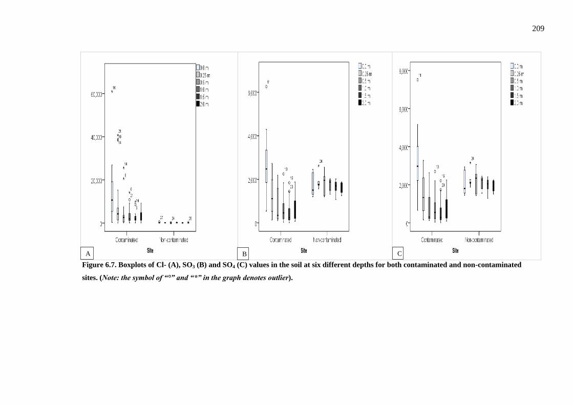
209
Figure 6.7. Boxplots of Cl- (A), SO3 (B) and SO4 (C) values in the soil at six different depths for both contaminated and non-contaminated
sites. (Note: the symbol of “°” and “*” in the graph denotes outlier).
A B C

210
Table 6.6. The significant differences of the variables of Cl-, SO3 and SO4 concentration (mg/kg) in the soil at six different depths between
contaminated and non-contaminated sites. (Note: outlier values were deleted in this table).
Depth (m) Variable Site Name N Median Mean SD Min Max Z U t-value p-value
0.0
Cl- Contaminated 22 10638 10493.2 7441.7 255 26950
-3.28 2.0 ----- 0.001* Non-contaminated 5 106 106 73.9 42 170
SO3 Contaminated 22 2442 2304.6 985.8 541 4303
----- ----- 1.92 0.05* Non-contaminated 5 1503 1754.2 583.4 1204 2450
SO4 Contaminated 22 2930 2763.4 1211.9 649 5162
----- --- 1.918 0.042* Non-contaminated 5 1804 2104.4 699.8 1445 2939
0.25
Cl- Contaminated 22 2837 4035.4 3747.1 43 15248
-2.95 6.0 ----- 0.001* Non-contaminated 5 113 90.2 57.919 28 141
SO3 Contaminated 22 1111 1248.8 907.3 129 2733
----- ----- -2.381 0.026* Non-contaminated 5 1746 1738.5 139.61 1561 1901
SO4 Contaminated 22 1333 1498.3 1088.52 155 3279
----- --- -2.491 0.026* Non-contaminated 5 2095 2086 167.5 1873 2281
0.5
Cl- Contaminated 22 1985.5 2123.1 2025.6 43 7518
-2.95 6.0 ----- 0.001* Non-contaminated 5 49 52.7 24.3 28 85
SO3 Contaminated 22 345.5 789.95 735.17 104 2187
----- ----- -2.904 0.008* Non-contaminated 5 1953 1816 583.76 1196 2554
SO4 Contaminated 22 306 861.04 854.70 125 2624
----- --- -3.203 0.004* Non-contaminated 5 2343 2180.8 697.9 1435 3064
1.0
Cl- Contaminated 22 1687.5 2127.1 1636.2 85 6525
-3.05 5.0 ----- 0.001* Non-contaminated 5 113 181 158.8 56 425
SO3 Contaminated 22 530 643.8 564.9 27 1841
----- ----- -4.804 0.001* Non-contaminated 5 1876 1736.2 322.79 1304 2036
SO4 Contaminated 22 471 672.52 622.85 33 2209
----- --- -5.605 0.001* Non-contaminated 5 2251 2082.6 387.6 1563 2442
1.5
Cl- Contaminated 22 1702 1843.1 1194.6 85 4255
-3.26 2 ----- 0.001* Non-contaminated 5 56 95.8 62.23 56 198
SO3 Contaminated 22 228 418.5 409.6 5 1422
----- ----- -7.013 0.001* Non-contaminated 5 1704 1627.8 369.11 1067 2014
SO4 Contaminated 22 273 467.4 453.9 7 1706
----- ----- -4.707 0.001* Non-contaminated 5 2044 1953 442.8 1280 2416
2.0
Cl- Contaminated 22 2269.5 3380.13 2723.28 57 9220
-2.98 2.00 ----- 0.001* Non-contaminated 5 70.5 67 21.55 42 85
SO3 Contaminated 22 307.5 588.18 530.44 71 1872
----- ----- -4.19 0.001* Non-contaminated 5 1753 1624 280.01 1256 1874
SO4 Contaminated 22 368.5 705.68 636.4 86 2246
----- ----- -4.190 0.001* Non-contaminated 5 2103 1948.2 335.64 1507 2248
Note, *p < .05 indicates to the significant difference in the variable between two different groups.

211
Figure 6.8. Comparing median values of Cl- concentration (mg/kg) in the soil at six different
depths between contaminated and non-contaminated site. (Note: Error bars denote 95 % lower
and upper confidence intervals).
Figure 6.9. Comparing mean values of SO3 concentration (mg/kg) in the soil at six different
depths between contaminated and non-contaminated site. (Note: Error bars denote standard
deviation).
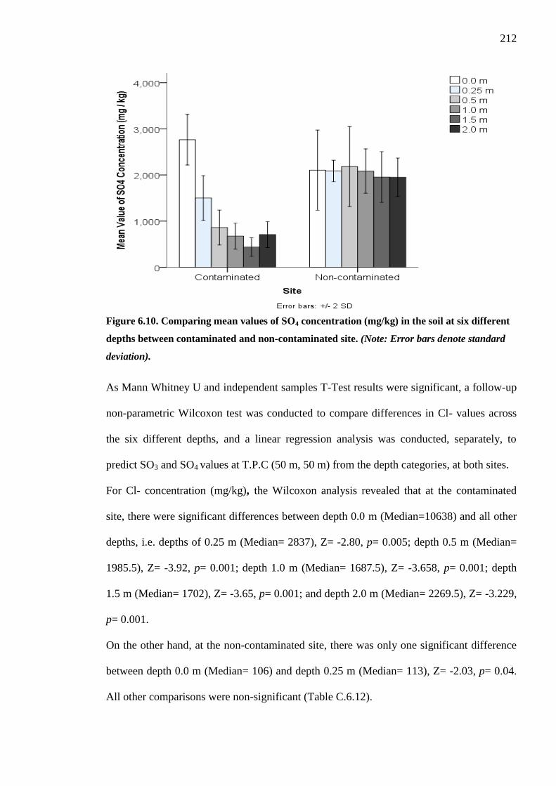
212
Figure 6.10. Comparing mean values of SO4 concentration (mg/kg) in the soil at six different
depths between contaminated and non-contaminated site. (Note: Error bars denote standard
deviation).
As Mann Whitney U and independent samples T-Test results were significant, a follow-up
non-parametric Wilcoxon test was conducted to compare differences in Cl- values across
the six different depths, and a linear regression analysis was conducted, separately, to
predict SO3 and SO4 values at T.P.C (50 m, 50 m) from the depth categories, at both sites.
For Cl- concentration (mg/kg), the Wilcoxon analysis revealed that at the contaminated
site, there were significant differences between depth 0.0 m (Median=10638) and all other
depths, i.e. depths of 0.25 m (Median= 2837), Z= -2.80, p= 0.005; depth 0.5 m (Median=
1985.5), Z= -3.92, p= 0.001; depth 1.0 m (Median= 1687.5), Z= -3.658, p= 0.001; depth
1.5 m (Median= 1702), Z= -3.65, p= 0.001; and depth 2.0 m (Median= 2269.5), Z= -3.229,
p= 0.001.
On the other hand, at the non-contaminated site, there was only one significant difference
between depth 0.0 m (Median= 106) and depth 0.25 m (Median= 113), Z= -2.03, p= 0.04.
All other comparisons were non-significant (Table C.6.12).
213
For SO3 content, linear regression showed that at both sites, depth does not predict SO3
concentration values, i.e. at the (contaminated site: B= -280.12, SEB = 282.19, Beta = -
0.44, p = 0.37 and at the non-contaminated site: B = -127.49, SEB =178.04, Beta = -0.337,
p = 0.51). It therefore shows that there is no significant association between depth and SO3
content at either site (Figure 6.11). Additionally, the results of SO4 content showed that the
depth does not predict SO4 concentration values (contaminated site: B= 336.21, SEB=
338.63, Beta= -0.44, p= 0.37; non-contaminated site: B= 153.13, SEB= 213.60, Beta= -
0.33, p= 0.51). Hence, it can be stated that there is no significant relationship between
depth and SO4 values at both sites at T.P.C. (50 m, 50 m) (Figure 6.12).
These results mean that the depth at certain points cannot predict the concentrations of SO3
and SO4 at either site.

214
Figure 6.11. Scatterplot showing relationship between six different depths and SO3
concentration (mg/kg) at T.P.C (50 m, 50 m), at contaminated site (A) and non-contaminated
site (B).
B
A

215
Figure 6.12. Scatterplot showing relationship between six different depths and SO4
concentration (mg/kg) at T.P.C (50 m, 50 m), at contaminated site (A) and non-contaminated
site (B).
A
B
216
6.4 Vario Macro Elemental Analyses (EA)
6.4.1 Laboratory Results of EA
Tables C.6.13 to C.6.18 present the Elemental Analysis (EA) test results for the soil
samples taken from the contaminated site; the results for similar tests performed on
samples obtained from the non-contaminated site are shown in Table C.6.19. Similarly, the
maximum, minimum, standard deviation and mean values were calculated and tabulated
against the depth.
Tables 6.7 and 6.8 show the mean percentage values of nitrogen, carbon, sulphur and
hydrogen against the layer depths for contaminated and non-contaminated sites. Figure
6.13 shows how the carbon percentage changes with the depth at the contaminated site.
The followings should be noted from Tables (6.7 & 6.8) and figure (6.13):
(a) The carbon content was very high (nearly 21 %) at the top layer of
the contaminated site. It however, decreased sharply with depth down
to 0.5 m where it reached nearly 2 % and a further slight decrease was
recorded down to 2.0 m. On the other hand, at the non-contaminated
site a negligible carbon content was clearly shown, (as shown in Table
6.8) even at the top layer.
(b) Nearly the same trend of changes in the carbon, as discussed above,
was noted for the changes of Nitrogen, Sulphur and Hydrogen with the
depth, although the concentrations of these materials were low even at
the top layer of the contaminated site as compared with the carbon
content. The lower values of these materials were expected as the oil
itself mostly contains hydrogen and carbon and the hydrogen mostly
evaporates when exposed to the air and high sun temperatures.
However, at the non-contaminated site, these materials were negligible.

217
Table 6.7. Mean percentages values of Nitrogen, Carbon, Sulphur and Hydrogen in soil
samples at six different depths in contaminated site.
Trial Pits Coordinates
(T.P.Cs)
Sample Weight (g)
Content of N, C, S & H (%) by elemental analysis N % C % S % H %
0.0 m 45.40 0.54 20.86 2.43 2.72 0.25 m 45.95 0.45 8.33 0.97 1.10 0.5 m 44.56 0.26 2.12 0.09 0.02 1.0 m 45.49 0.39 2.12 0.10 0.07 1.5 m 44.94 0.21 1.59 0.12 0.02 2.0 m 45.06 0.14 0.62 0.09 0.01
Table 6.8. Mean percentages values percentages of Nitrogen, Carbon, Sulphur and
Hydrogen in soil samples at two different depths (0.0 m, 0.25 m) in non-contaminated site.
Trial Pits Coordinates (T.P.Cs)
Sample Weight (g)
Content of N, C, S & H (%) by elemental analysis Nitrogen
N % Carbon
C % Sulphur
S % Hydrogen H
% 0.0 m 36.79 0.0027 0.048 0.008 0.0054
0.25 m 44.96 0.00026 0.00066 0.001 0.0011
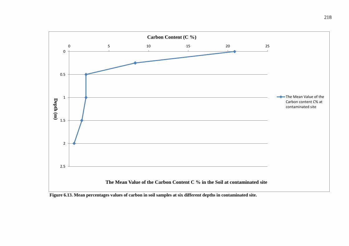
218
Figure 6.13. Mean percentages values of carbon in soil samples at six different depths in contaminated site.
0
0.5
1
1.5
2
2.5
0 5 10 15 20 25
Depth (m
)
Carbon Content (C %)
The Mean Value of the Carbon Content C % in the Soil at contaminated site
The Mean Value of theCarbon content C% atcontaminated site

219
6.4.2 Statistical Summary of EA
Figures 6.14 and 6.15 shows the outliers present in the nitrogen (N %), carbon (C %),
sulphur (S %) and hydrogen (H %) data for the contaminated site only, as the N %, C %, S
% and H % data had low percentage values at depths 0.0 m and 0.25 m and were not
detected at other depths in non-contaminated site. Outliers in the contaminated data were
deleted prior to analysis. The C %, N % and S % data had normal distributions. However,
the H % data were skewed; therefore non-parametric tests were performed on this data.
(Tables C.6.20 and C.6.21)
Table 6.9 shows the independent samples T-Test results for C %, N % and S % data, and
Mann Whitney U results for the H % data, at both sites at the two depths of 0.0 m and 0.25
m (Tables C.6.22 and C.6.23). The T-Test showed significant differences in mean
percentage values of C % (at depth 0.0 m, t(25) = 4.83, p= 0.002; at depth 0.25 m, t(21) =
4.65, p= 0.001); N % (at depth 0.0 m, t(25) = 17.05, p= 0.001; at depth 0.25 m, t(25) =
19.41, p= 0.001) and S % (at depth 0.0 m, t(21) = 7.48, p= 0.001, at depth 0.25 m, t(19) =
4.32, p= 0.001) (Figure 6.16).
The Mann Whitney U analysis found significant differences in median percentage values
of H % between contaminated and non-contaminated sites at the two depths investigated:
0.0 m (Z= -3.43, U= 0.000, p= 0.001) and 0.25 m (Z= -3.41, U= 0.00, p= 0.001) (Figure
6.17).
The above results show that the statistical analysis (after deleting the outliers from the
mean/median values) do not much change the general values found in tables 6.8 and 6.9,
i.e. it does not much vary the trend towards the concentration of elements against the
depths. Furthermore, it indicates that the oil spill contamination is responsible for the
existence of these element materials at the contaminated site.

220
Figure 6.14. Boxplots of N % (A) and C % (B) percentages values in the soil at six different depths for contaminated site. (Note: the symbol of “*”
and “°” in the graph denotes outlier).
A B

221
Figure 6.15. Boxplots of S % (A) and H % (B) percentages values in the soil at six different depths for contaminated site. (Note: the symbol of “*”
and “°” in the graph denotes outlier).
A B

222
Table 6.9. The significant differences of the variables of elemental analysis (N %, C %, H % & S %) at two different depths (0.0 m & 0.25
m) between contaminated and non-contaminated sites. (Note: outlier values were deleted in this table).
Depth (m)
Variable Site Name N Median Mean SD Min Max Z U t-value p-value
0.0
N% Contaminated 22 0.57 0.56 0.059 0.446 0.652
------- ------- 17.05 0.001* Non-contaminated 5 0.0029 0.0030 0.0006 0.0025 0.0037
C% Contaminated 22 23.275 20.86 9.485 4.058 37.58
------- ------- 4.83 0.001* Non-contaminated 5 0.036 0.048 0.036 0.01 0.09
H% Contaminated 22 3.00 2.64 1.36 0.37 5.19
-3.43 0.00 ------- 0.001* Non-contaminated 5 0.0052 0.0054 0.0029 0.0 0.01
S% Contaminated 22 2.81 2.47 1.57 0.49 5.15
------- ------- 7.48 0.001* Non-contaminated 5 0.008 0.008 0.0056 0.001 0.014
0.25
N% Contaminated 22 0.439 0.450 0.050 0.387 0.556
------- ------- 19.41 0.001* Non-contaminated 5 0.0 0.0003 0.00053 0.0 0.0
C% Contaminated 22 6.698 8.333 8.405 0.516 30.77
------- ------- 4.65 0.001* Non-contaminated 5 0.001 0.0007 0.0006 0.0 0.0
H% Contaminated 22 0.6270 0.9904 1.096 0.039 3.6550
-3.41 0.00 ------- 0.001* Non-contaminated 5 0.001 0.0012 0.0007 0.0 0.0
S% Contaminated 22 0.479 0.649 0.839 0.173 3.617
------- ------- 4.32 0.001* Non-contaminated 5 0.0 0.001 0.001 0.0 0.003
0.5**
N% Contaminated 22 0.2595 0.2597 0.0070 0.2480 0.2710 ------- ------- ------- ------- C% Contaminated 22 2.27 2.129 0.446 0.546 2.669 ------- ------- ------- ------- H% Contaminated 22 0.022 0.022 0.0026 0.0180 0.0270 ------- ------- ------- ------- S% Contaminated 22 0.0710 0.0993 0.0700 0.053 0.346 ------- ------- ------- -------
1.0**
N% Contaminated 22 0.4255 0.4225 0.0586 0.2460 0.4980 ------- ------- ------- ------- C% Contaminated 22 2.177 2.124 0.246 1.593 2.553 ------- ------- ------- ------- H% Contaminated 22 0.046 0.0488 0.0259 0.017 0.096 ------- ------- ------- ------- S% Contaminated 22 4.499 3.91784 3.212 0.125 9.100 ------- ------- ------- -------
1.5**
N% Contaminated 22 0.2050 0.2058 0.0340 0.1370 0.2560 ------- ------- ------- ------- C% Contaminated 22 2.251 2.198 0.2480 1.365 2.538 ------- ------- ------- ------- H% Contaminated 22 0.019 0.020 0.0075 0.013 0.035 ------- ------- ------- ------- S% Contaminated 22 0.0530 0.1338 0.223 0.026 0.953 ------- ------- ------- -------
2.0**
N% Contaminated 22 0.139 0.1389 0.0367 0.0690 0.2050 ------- ------- ------- ------- C% Contaminated 22 0.726 0.628 0.291 0.037 1.145 ------- ------- ------- ------- H% Contaminated 22 0.0100 0.0102 0.0041 0.0030 0.0180 ------- ------- ------- ------- S% Contaminated 22 0.0310 0.1076 0.2003 0.011 0.805 ------- ------- ------- -------
Note, *p < .05 indicates to the significant difference in the variable between two different groups. ** No further deteced percentages values of N %, C %, H % and S % at depths 0.5 m, 1.0 m, 1.5 m and 2.0 m in non-contaminated site.
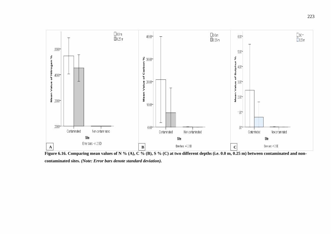
223
Figure 6.16. Comparing mean values of N % (A), C % (B), S % (C) at two different depths (i.e. 0.0 m, 0.25 m) between contaminated and non-
contaminated sites. (Note: Error bars denote standard deviation).
A B C

224
Figure 6.17. Comparing median percentages values of H % at two different depths (in
metres) between contaminated and non-contaminated sites. (Note: Error bars denote 95%
lower and upper confidence intervals).
The C %, N % and S % predictors were entered individually into three separate linear
regression models to examine their contribution towards predicting depth degrees in the
contaminated site at T.P.C. (50 m, 50 m). The results revealed that the depth was a
significant of N % (B= -0.13, SEB= 0.04, Beta= 0.83, p= 0.03). For every one meter
increase in depth, N % decreased by 0.139 degrees. The R Square value of 0.699 indicates
that depth accounted for approximately 69.9 % of the Nitrogen % in the contaminated data.
On the other hand, the depth was not found to be significant for predicating the carbon %
(B= -4.49, SEB= 3.00, Beta= -0.59, p= 0.20) and sulphur % (B= -0.98, SEB= 0.67, Beta= -
0.58, p= 0.22) (Figure 6.18).

225
For H % percentage values, the Wilcoxon analysis revealed that there was a significant
difference between depth 0.0 m (Median = 3.08) and all other depths, including depth 0.25
m (Median = 0.65), Z= -3.12, p= 0.002; depth 0.5m (Median = 0.02), Z= -4.10, p= 0.001);
depth 1.0 m (Median = 0.05), Z= -4.10, p= 0.001); depth 1.5 m (Median = 0.02), Z= -4.10,
p= 0.001); and 2.0 m (Median = 0.01), Z= -4.10, p= 0.001). Note that the Z value and
statistical significance shows an identical difference between 0.0 m depth and 0.5 m to 2.0
m depths (Table C.6.24).
From the above, it can be claimed that the depth is significant in predicating N % and H %
but not significant for predicating S % and C % contents.

226
Figure 6.18. Scatterplot showing relationship between six different depths and N % (A), C % (B) and S % (C) percentages at T.P.C (50 m, 50 m),
at contaminated site.
A B C

227
6.5 Gas Chromatograph Mass Spectrometry (GC-MS)
6.5.1 Laboratory Results of GC-MS
Of the 22 tested samples extracted from the hydrocarbon contamination site, the total
number found to be contaminated with TPH are shown in Table 6.10.
The findings from the GC-MS tests, e.g. the TPH concentration (mg/kg) and chemical
composition, conducted on samples detected with TPH obtained from the contaminated
(dry oil lake) site taken at depths of 0.0 m, 0.25 m and 0.5 m below ground, are shown in
appendix C; Tables C.6.25 to C.6.47 and Figures C.6.1 to C.6.23. One example of a
sample detected with TPH from T.P.C of (0 m, 25 m) at 0.0 m depth via GC-MS
instrument is shown in Table 6.11 and Figure 6.19.
As clarified in chapter 2 (section 2.7, p. 36), the contaminated site in this study resulted
from crude oil spills from the Iraqi invasion, - more than 26 years ago - therefore, this
petroleum hydrocarbon contaminant mixtures has been subjected to the time factor which
has caused several alterations through weathering (dissolution or evaporation), chemical
degradation (effects of sunlight, heat, and air and soil chemistry) and biological alteration
(impact of microorganisms).
Figure 6.19 represents the total ion chromatogram (TIC) of typical soil contaminated
samples analysed by the GC-MS test; i.e. results were obtained through sample injected
into the GC-MS system for subsequent separation and identification according to their
boiling point and characteristic mass fragments, respectively. Whereas, TIC displayed of
typical compounds which might be related to: paraffin’s mono aromatics; bi aromatics; or
tri aromatic; which these substances are related to in TPH terms. For example, all the
chemical compositions detected in contaminated soil samples for T.P.C. (0 m, 25 m) at a
depth of 0.0 m via the GC-MS instrument, belong to paraffin’s compounds (considered to
be part of the TPH) (Table 6.11 & Figure 6.19).

228
Therefore, figure 6.19, clearly shows a hump and spiky peak of individual compounds
which represent a TPH composition of around 19.8 to 24.2 minutes of retention time for
contaminated samples.
The GC-MS results for samples taken from the contaminated site but not detected with
TPH are shown in figures C.6.24 up to C.6.108 at depths of 0.0 m, 0.25 m, 0.5 m, 1.0 m
and 1.5 m belowground. Figure 6.20 illustrates an example of the result of a sample found
without any TPH for T.P.C. (0 m, 0 m) at a depth of 0.0 m. On the other hand, the GC-MS
results for samples obtained from the non-contaminated site are displayed in figures
C.6.109 to C.6.117. An example of one control sample for T.P.C. (50 m, 50 m) at 0.0 m
depth is given in Figure 6.21.
The TPH concentrations (mg/kg) detected in contaminated samples (contaminated site) at
depths of 0.0 m, 0.25 m and 0.5 m are shown in Tables C.6.48 to C.6.50. The same tables
(C.6.48 to C.6.50) also exhibit the minimum, maximum, mean and standard deviation
values of TPH (mg/kg) for samples obtained from depths of 0.0 m, 0.25 m, 0.5 m.
Table 6.12 and Figure 6.22 show the mean values of TPH concentration against the layer
depth for both contaminated and non-contaminated sites. The Table indicates that the
highest TPH value was in the top layer of the contaminated site recording 257.8 mg/kg.
However, this decreases dramatically at depths reaching 103.6 mg/kg at 0.25 m depth and
1.0 mg/kg at 0.5 m depth. It was not detected at lower depths. The table also shows that the
TPH was not detected at the non-contaminated site which confirms that the non-
contaminated site has not been contaminated with hydrocarbon.
Similar tests were carried out in other areas using the (GC-MS) technique, Al-Sarawi et al.
(1998b) used the GC-MS technique on hydrocarbon contaminated soils in the Al-Ahmadi
and Greater Burgan Oil Fields and have found that soils in both regions had high
concentrations of TPH. The soil from the Al-Ahmadi profile was found to have high TPH
even at greater depths (80-95 cm) whereas the soil from the Burgan Oil Fields had high
229
levels of TPH only on the surface (upper 50 cm layer). The results at the Burgan Field
study very closely matched those of the present study where depth of influence for
hydrocarbon contaminated soil in the Greater Burgan Field was also found to be 0.5 m
from the surface.
Additionally, Okop and Ekpo (2012) investigated the spillage of crude oil which
contaminated the soil within the Nigeria’s Niger Delta area, approximately three months
after that major incidence. Samples of soil were extracted from depths of 0.0 m to 0.15 m,
0.15 m to 0.3 m and 0.30 m to 0.60 m belowground; the samples were examined using GC
equipped with a device to detect flame ionisation. The result showed that the TPH
concentrations for the topsoil, sub-soil and lowest depth measured were 9 – 289 mg/kg, 8 –
318 mg/kg and 7 – 163 mg/kg respectively. It also indicated that the levels of total
hydrocarbon contents were higher in comparison with the reference site. The results prove
that there is an urgent need to develop a complete and sustainable remediation and
monitoring plan for the environment.
Pathak et al. (2011) investigated the effect of petroleum oil on the soil in the Jaipur area
(India). Soil samples were taken at a depth of 60 mm below ground close to the India
Motor Garage in Transport Nagar India. Chemical analysis of soil was performed using the
GC-MS test in order to find the TPH concentration in the soil samples from two different
sites, i.e. contaminated & non-contaminated areas. They observed significantly high TPH
concentrations in soils from the contaminated site as compared to the non-contaminated
site.
Thus, the present study is also in line with past studies, and has confirmed the hydrocarbon
contamination at the contaminated dry oil lake site; also showing that the top 50 cm of
depth is an effective zone of contamination with hydrocarbon presence (Table 6.12 and
Figure 6.22).

230
Table 6.10. Number of detected and not detected samples with TPH tested by GC-MS test at
contaminated site.
Depth (m)
Total Number of Samples Detected with Total Petroleum Hydrocarbons (TPH)
out of 22 Samples Collected at each Depth
The Percentage of the Detected Samples out of
the Total 22 Samples.
0.0 m 16 73.00 % 0.25 m 7 32.00 % 0.5 m 1 5.0 % 1.0 m ND* ND* 1.5 m ND* ND*
Note: ND*: not detected with petroleum hydrocarbon.

231
Table 6.11. An example shows the results for one of the detected sample with TPH which tested by GC-MS instrument for T.P.C (0 m, 25 m) at depth
(0.0 m) of contaminated site.
Peak Ret. Time
Chemical Composition of the TPH in the
Contaminated Soil Sample
Area Under the Curve (m2)
Chemical Composition
Formula
Classification of the
TPH Substance based on Aliphatic or
Aromatic
Concentration of each TPH
Chemical Composition Detected in
the Contaminated
Soil Sample (µg/ml)
Concentration of each TPH Chemical
Composition Detected in the Contaminated
Soil Sample (mg/kg)
Total
Concentration of the Total
TPH Compositions
Detected in the Contaminated
Soil Sample (mg/kg)
References
1*2 2.462 PV --------- 5656160 --------- --------- 46.62 15.54
352.37
---------
2*1 19.875 PV 2-Methyldodecane 6480023 C13H28 Aliphatic C12-C16 57.30 19.1 (Two-Methyldodecane, n.d.)
3*1 20.311 PV Tetramethylpentadecane 7042148 C19H40 Aliphatic C16-C35 64.56 21.52 (Pristane, n.d.)
4*1 21.069 VV Tetramethylhexadecane 14937449 C20H42 Aliphatic C16-C35 166.812 55.604 (Two, 6, 10, 14-
tetramethylhexadecane, n.d.) 5*1 21.689 VV Nonadecane 7206111 C19H40 Aliphatic C16-C35 66.70 22.233 (Nonadecane, n.d.)
6*1 21.970 PV Dimethylhexadecane 5585519 C18H38 Aliphatic C16-C35 45.70 15.233 (Two, 2-dimethylhexadecane,
n.d.) 7*2 22.172 VV --------- 5274027 --------- --------- 41.67 13.89 ---------
8*1 22.349 VV Eicosane 14529974 C20H42 Aliphatic C16-C35 161.53 53.843 (Icosane, n.d.)
9*1 22.608 VV Eicosane 4485710 C20H42 Aliphatic C16-C35 31.46 10.486 (Icosane, n.d.)
10*1 22.643 VV Pentadecane 6449501 C15H32 Aliphatic C12-C16 56.89 18.963 (Pentadecane, n.d.)
11*1 22.844 VV 9,10-
Dimethylanthracene 13104405 C16H14 Aromatic C16-C21 143.07 47.69
(Nine, 10-dimethylanthracene, n.d.)
12*1 22.981 VV Heneicosane 13477178 C21H44 Aliphatic C16-C35 147.90 49.3 (Heneicosane, n.d.)
13*1 23.595 PV Docosane 8978255 C22H46 Aliphatic C16-C35 89.64 29.88 (Docosane, n.d.)
14*1 24.258 PV Octadecane 4029007 C18H38 Aliphatic C16-C35 25.547 8.515 (Octadecane, n.d.)
Notes: 1*Brown colour clarify the hydrocarbon compounds and their concentrations detected in soil sample. 2* Blue Colure clarify the unknown chemical compounds and their concentrations (not identified by diesel standard) detected in soil sample which are excluded
from the total concentration of the TPH.
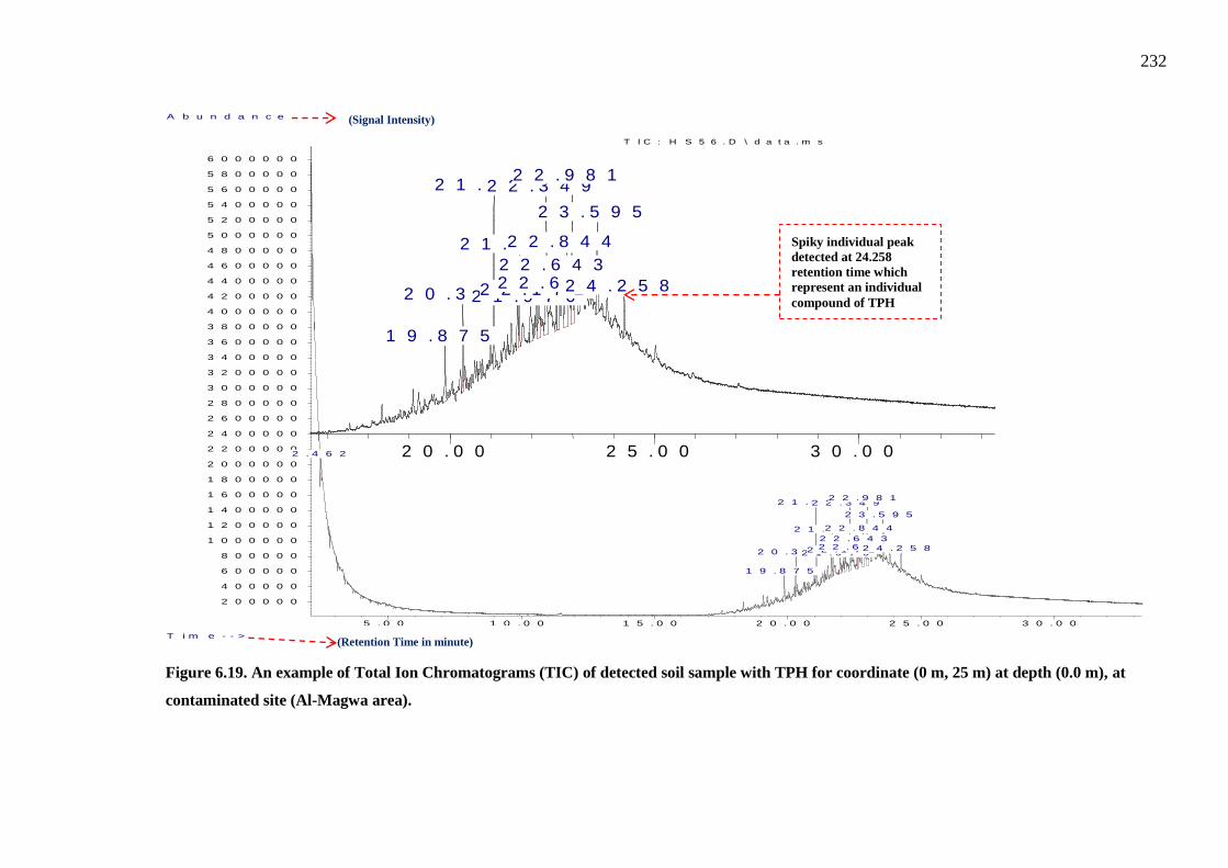
232
Figure 6.19. An example of Total Ion Chromatograms (TIC) of detected soil sample with TPH for coordinate (0 m, 25 m) at depth (0.0 m), at
contaminated site (Al-Magwa area).
5 . 0 0 1 0 . 0 0 1 5 . 0 0 2 0 . 0 0 2 5 . 0 0 3 0 . 0 0
2 0 0 0 0 0
4 0 0 0 0 0
6 0 0 0 0 0
8 0 0 0 0 0
1 0 0 0 0 0 0
1 2 0 0 0 0 0
1 4 0 0 0 0 0
1 6 0 0 0 0 0
1 8 0 0 0 0 0
2 0 0 0 0 0 0
2 2 0 0 0 0 0
2 4 0 0 0 0 0
2 6 0 0 0 0 0
2 8 0 0 0 0 0
3 0 0 0 0 0 0
3 2 0 0 0 0 0
3 4 0 0 0 0 0
3 6 0 0 0 0 0
3 8 0 0 0 0 0
4 0 0 0 0 0 0
4 2 0 0 0 0 0
4 4 0 0 0 0 0
4 6 0 0 0 0 0
4 8 0 0 0 0 0
5 0 0 0 0 0 0
5 2 0 0 0 0 0
5 4 0 0 0 0 0
5 6 0 0 0 0 0
5 8 0 0 0 0 0
6 0 0 0 0 0 0
T i m e - - >
A b u n d a n c e
T I C : H S 5 6 . D \ d a t a . m s
2 . 4 6 2
1 9 . 8 7 5
2 0 . 3 1 1
2 1 . 0 6 9
2 1 . 6 8 9
2 1 . 9 7 02 2 . 1 7 2
2 2 . 3 4 9
2 2 . 6 0 82 2 . 6 4 32 2 . 8 4 4
2 2 . 9 8 1
2 3 . 5 9 5
2 4 . 2 5 8
(Signal Intensity)
(Retention Time in minute)
Spiky individual peak detected at 24.258 retention time which represent an individual compound of TPH
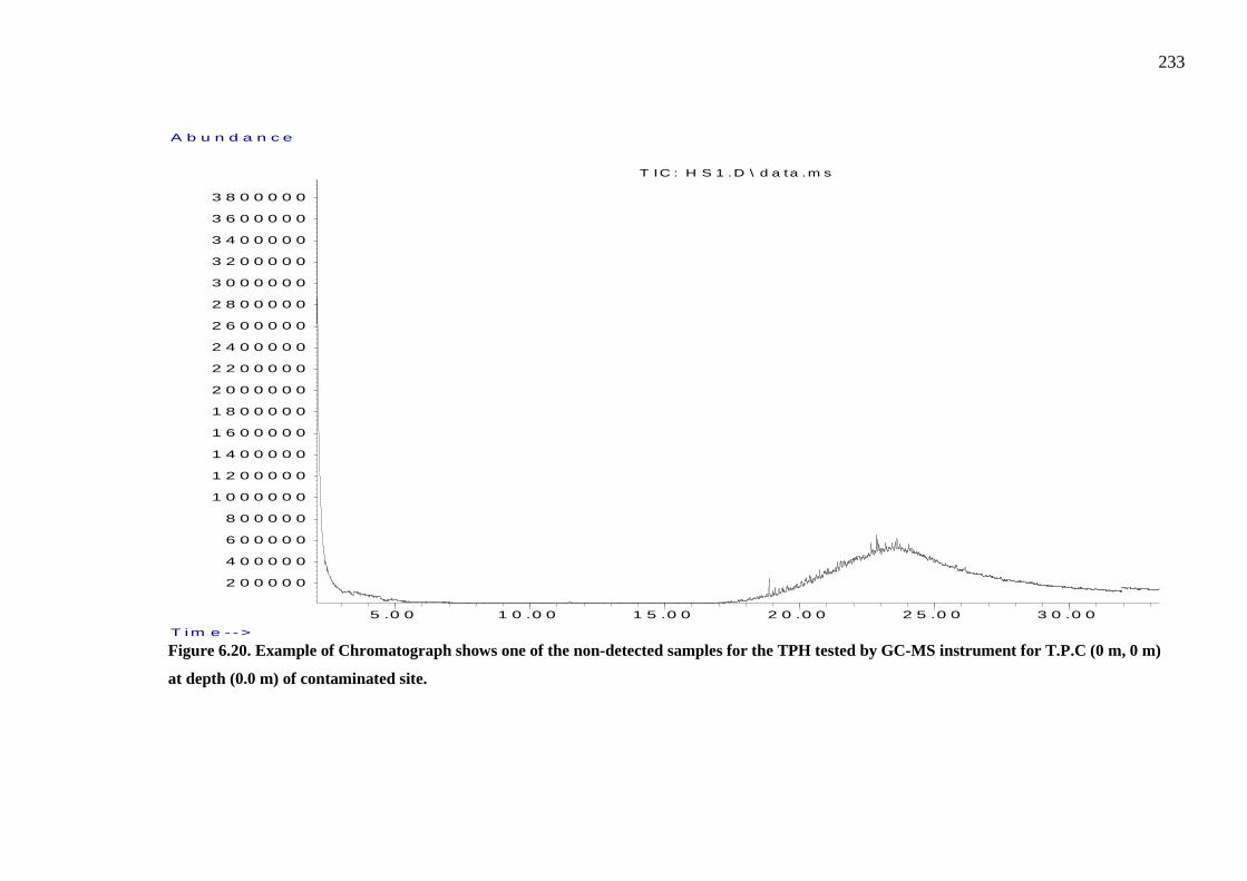
233
Figure 6.20. Example of Chromatograph shows one of the non-detected samples for the TPH tested by GC-MS instrument for T.P.C (0 m, 0 m)
at depth (0.0 m) of contaminated site.
5 .0 0 1 0 .0 0 1 5 .0 0 2 0 .0 0 2 5 .0 0 3 0 .0 0
2 0 0 0 0 0
4 0 0 0 0 0
6 0 0 0 0 0
8 0 0 0 0 0
1 0 0 0 0 0 0
1 2 0 0 0 0 0
1 4 0 0 0 0 0
1 6 0 0 0 0 0
1 8 0 0 0 0 0
2 0 0 0 0 0 0
2 2 0 0 0 0 0
2 4 0 0 0 0 0
2 6 0 0 0 0 0
2 8 0 0 0 0 0
3 0 0 0 0 0 0
3 2 0 0 0 0 0
3 4 0 0 0 0 0
3 6 0 0 0 0 0
3 8 0 0 0 0 0
T im e - ->
A b u n d a n c e
T IC : H S 1 .D \ d a ta .m s

234
Figure 6.21. Example of Chromatograph shows one of the control sample tested by GC-MS instrument for T.P.C (50 m, 50 m) at depth (0.0 m)
of control site.
5 . 0 0 1 0 . 0 0 1 5 . 0 0 2 0 . 0 0 2 5 . 0 0 3 0 . 0 0
1 0 0 0 0 0
2 0 0 0 0 0
3 0 0 0 0 0
4 0 0 0 0 0
5 0 0 0 0 0
6 0 0 0 0 0
7 0 0 0 0 0
8 0 0 0 0 0
9 0 0 0 0 0
1 0 0 0 0 0 0
1 1 0 0 0 0 0
1 2 0 0 0 0 0
1 3 0 0 0 0 0
1 4 0 0 0 0 0
1 5 0 0 0 0 0
1 6 0 0 0 0 0
1 7 0 0 0 0 0
1 8 0 0 0 0 0
1 9 0 0 0 0 0
2 0 0 0 0 0 0
2 1 0 0 0 0 0
2 2 0 0 0 0 0
2 3 0 0 0 0 0
2 4 0 0 0 0 0
2 5 0 0 0 0 0
2 6 0 0 0 0 0
2 7 0 0 0 0 0
2 8 0 0 0 0 0
2 9 0 0 0 0 0
3 0 0 0 0 0 0
T i m e - - >
A b u n d a n c e
T I C : H S 1 1 . D \ d a t a . m s

235
Table 6.12. Mean values of the TPH concentration (mg/kg) in the soil samples at
contaminated and non-contaminated site at different depths.
Depth
(m)
The Mean Value of the TPH Concentration in the Soil Samples (mg/kg)
At Contaminated site At Non-contaminated site
0.0 257.80 0 0.25 103.65 0 0.5 1.0 0 1.0 0 0 1.5 0 0 2.0 0 0
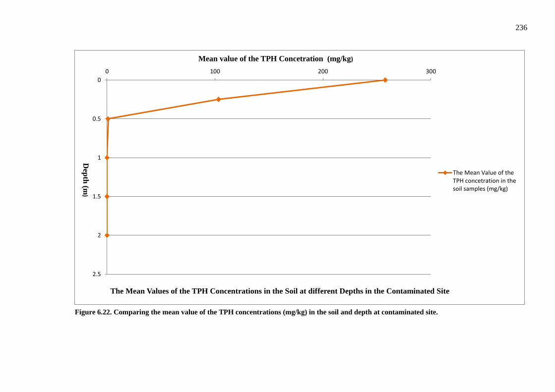
236
Figure 6.22. Comparing the mean value of the TPH concentrations (mg/kg) in the soil and depth at contaminated site.
0
0.5
1
1.5
2
2.5
0 100 200 300
Depth (m
)
Mean value of the TPH Concetration (mg/kg)
The Mean Values of the TPH Concentrations in the Soil at different Depths in the Contaminated Site
The Mean Value of theTPH concetration in thesoil samples (mg/kg)
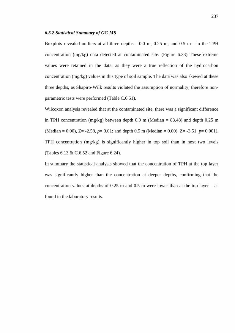
237
6.5.2 Statistical Summary of GC-MS Boxplots revealed outliers at all three depths - 0.0 m, 0.25 m, and 0.5 m - in the TPH
concentration (mg/kg) data detected at contaminated site. (Figure 6.23) These extreme
values were retained in the data, as they were a true reflection of the hydrocarbon
concentration (mg/kg) values in this type of soil sample. The data was also skewed at these
three depths, as Shapiro-Wilk results violated the assumption of normality; therefore non-
parametric tests were performed (Table C.6.51).
Wilcoxon analysis revealed that at the contaminated site, there was a significant difference
in TPH concentration (mg/kg) between depth 0.0 m (Median = 83.48) and depth 0.25 m
(Median = 0.00), Z= -2.58, p= 0.01; and depth 0.5 m (Median = 0.00), Z= -3.51, p= 0.001).
TPH concentration (mg/kg) is significantly higher in top soil than in next two levels
(Tables 6.13 & C.6.52 and Figure 6.24).
In summary the statistical analysis showed that the concentration of TPH at the top layer
was significantly higher than the concentration at deeper depths, confirming that the
concentration values at depths of 0.25 m and 0.5 m were lower than at the top layer – as
found in the laboratory results.

238
Figure 6.23. Boxplots of TPH concentrations values (mg/kg) in the soil for contaminated site.
(Note: the symbol of “*” and “°” in the graph denotes outlier).
Table 6.13. The significant differences of the TPH variable in the soil between different
depths (0.0 m, 0.25 m & 0.5 m) at contaminated site.
Depth (m) N Mean Median SD Min Max Z (0.0 m-
0.25 m) Z (0.0 m-
0.5 m) 0.0 22 257.15 83.48 345.77 0.00 1330.08
-2.58
-3.51 0.25 22 103.65 0.00 289.20 0.00 1271.03
0.5 22 0.99 0.00 4.66 0.00 21.86
p-value 0.010* 0.001*
Note, *p < .05 indicates to the significant difference in the variable between two different groups.

239
Figure 6.24. Comparing the median values of TPH concentration (mg/kg) between different
depths (i.e. 0.0 m, 0.25 m & 0.5 m) at contaminated site. (Note: Error bars denote 95 % lower
and upper confidence intervals).
240
6.5.3 Spatial Modelling of GC-MS Results (Contour Map)
The TPH concentrations (mg/kg) detected in contaminated samples (contaminated site) at
depths of 0.0 m, 0.25 m and 0.5 m are shown in Figures of contour maps 6.25 to 6.30. The
contour maps demonstrate the concentration of oil spillage (mg/kg) based on three
contrasting colours; this was carried out according to the TPH value recommended by the
U.S. EPA for soil clean-up (exceeding 100 mg/kg).
As such the TPH values of higher than 100 mg/kg are represented by the colour brown.
The yellow signifies the detected samples with TPH values of below 100 mg/kg and more
than the limit of TPH detection (in accordance with U.S EPA which states that such
concentrations does not need clean-up). White indicates the limit of detection samples with
TPH.
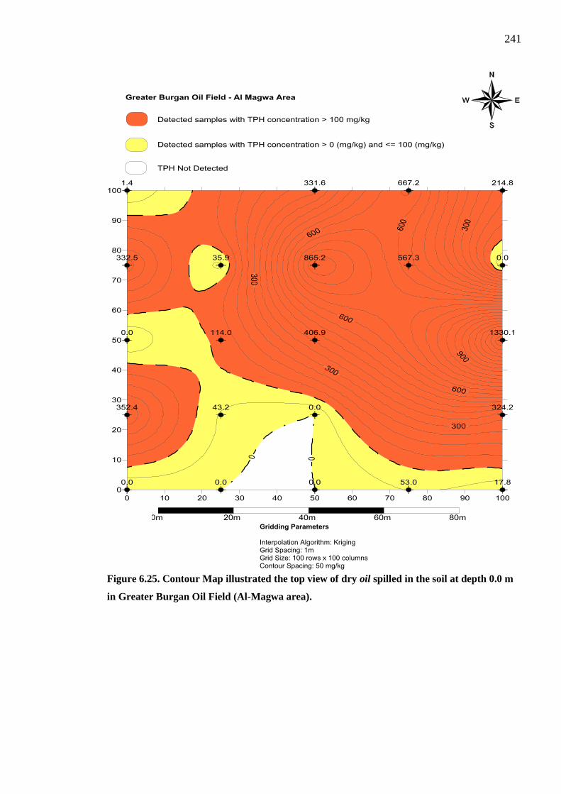
241
Figure 6.25. Contour Map illustrated the top view of dry oil spilled in the soil at depth 0.0 m
in Greater Burgan Oil Field (Al-Magwa area).
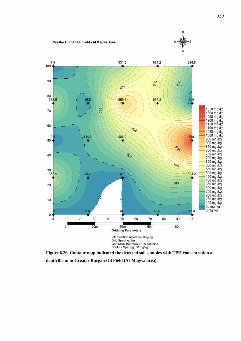
242
Figure 6.26. Contour map indicated the detected soil samples with TPH concentration at
depth 0.0 m in Greater Burgan Oil Field (Al-Magwa area).
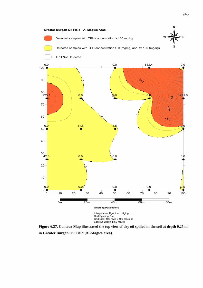
243
Figure 6.27. Contour Map illustrated the top view of dry oil spilled in the soil at depth 0.25 m
in Greater Burgan Oil Field (Al-Magwa area).
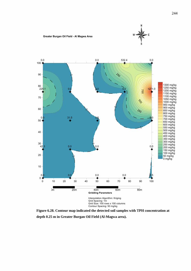
244
Figure 6.28. Contour map indicated the detected soil samples with TPH concentration at
depth 0.25 m in Greater Burgan Oil Field (Al-Magwa area).
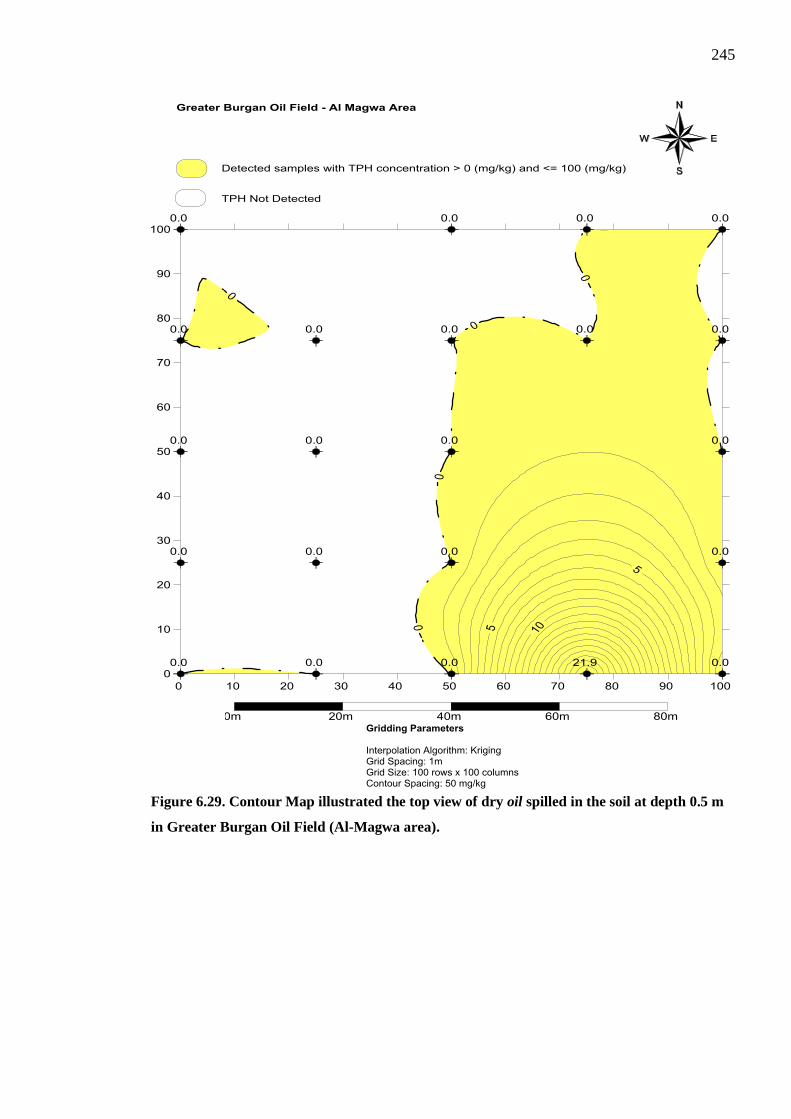
245
Figure 6.29. Contour Map illustrated the top view of dry oil spilled in the soil at depth 0.5 m
in Greater Burgan Oil Field (Al-Magwa area).
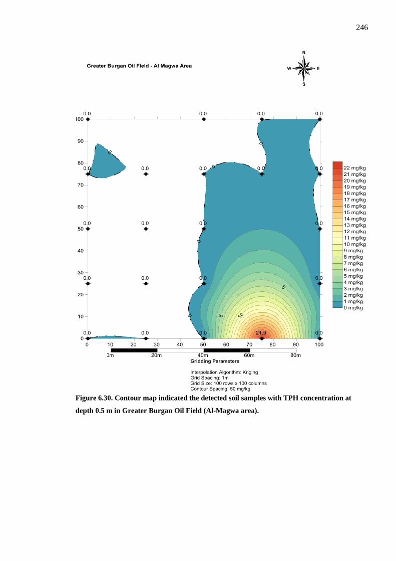
246
Figure 6.30. Contour map indicated the detected soil samples with TPH concentration at
depth 0.5 m in Greater Burgan Oil Field (Al-Magwa area).
247
6.6 Summary This Chapter has presented the findings of the geochemical characteristics of soil samples
taken from two different locations of the contaminated (dry oil lake) and the non-
contaminated sites. All the findings of the geochemical characterisation of soil were
undertaken to a statistical analysis. The investigated properties were pH, water soluble Cl-,
SO3 and SO4 content, EA (i.e. N %, C %, S % & H %) and GC-MS (i.e. TPH content)
analysis. The following conclusions were drawn from these analyses:
The difference between minimum and maximum pH values from the
hydrocarbon contaminated site was higher than those from the non-
contaminated site. Additionally, the minimum values of pH decreased due to
contamination. Statistical analysis proved the above findings, i.e. after
deleting outlier values.
Cl- concentration was very high at the top layer of the hydrocarbon
contaminated site and then decreased at depths lower than 0.5 m. However,
at the non-contaminated site, the chloride concentration was approximately
zero. Statistical analysis proved that there was a significant difference in Cl-
concentration between contaminated and non-contaminated sites.
Furthermore, there was significant difference in Cl- concentration between
depth 0.0 m and all other depths at contaminated site, while, there was only
one significant difference between depth 0.0 m and 0.25 m at non-
contaminated site.
In terms of SO3 and SO4, concentrations were found to be higher only at the
top soil layer of the hydrocarbon contaminated site than the non-
contaminated site. At depths lower than 0.25 m in the contaminated site,

248
however, both SO3 & SO4 dropped down suddenly to become lower than
that in the non-contaminated site. The concentration was then further
decreased (at the hydrocarbon contaminated site) at lower depths until it
reached approximately a constant value between 1.0 m and 2.0 m depths. At
the non-contaminated site the concentration of both sulphate types were
approximately constant throughout the depths. Statistical analysis confirmed
that the above finding was significantly true. While, statistically, no
relationship was found between the SO3 and SO4 content and the depth at
T.P.C. (50 m, 50 m) at both sites.
The C % content was very high in the top layer of the contaminated site.
However, it decreased sharply with depth. On the other hand, at the non-
contaminated site a negligible carbon content was shown even for the top
layer.
Nearly the same trend of changes in the C % content was noted regarding
the changes of N %, S % and H % contents with the depth levels; although
the concentrations of these materials were comparatively low even at the top
layer of the contaminated site as compared with the C % content. At the non-
contaminated site, however, these materials were negligible. Statistical
analysis proved that the mean percentage values of the N %, C % & S % and
median percentage of H % had significant differences between soil samples
taken the contaminated and non-contaminated sites. Additionally, the
percentage values of N % and H % in the soil at T.P.C. (50 m, 50 m) in the
contaminated site was found to be significantly decreased with the increase
in depth while no significant relationship was found between depth and S %
& C % contents.

249
The TPH value was higher in the top layer of the contaminated site but
decreased with depth down to 0.5 m; it was not detected at lower depths.
TPH was never detected at the non-contaminated site. Statistical analysis
proved that the TPH concentration had significant differences in the
contaminated soil between depths 0.0 m, 0.25 m and 0.5 m only.
The influence of ground hydrocarbon contamination on human health will be assessed in
the next Chapter. This will be done by classifying the pollutants in the hydrocarbon
contaminated soils into carcinogenic and non-carcinogenic categories as well as by
developing ‘ground modelling’ through obtaining the clean-up levels for this contaminated
site using RISC-5 software.
250
7. HUMAN HEALTH RISK ASSESSMENT (HHRA)
OF HYDROCARBON CONTAMINATED SOILS
7.1 Introduction
Petroleum Hydrocarbon Standards for Soil Clean-up are described in this chapter. Also, the
explanations of HHRA phases as follows: (1a), Hazard Identification (1b), Hazard
Assessment; (2a) Risk Estimation and (2b) Risk Evaluation are provided for the purpose of
applying these stages to the potential hydrocarbon contamination site (Al-Mgawa area)
showing how they have been adhered to.
The results of the HHRA carcinogenic and non-carcinogenic risk found in the soil samples
detected with hydrocarbon contamination (at dry oil lake) by means of RISC-5 modelling
software (Spence and Walden, 2001), will also be presented in this chapter.
This analysis was achieved through modelling the TPH aliphatic and aromatic
hydrocarbons fractions including their concentrations (mg/kg) of the detected samples
determined by the GC-MS test as well as some hydrocarbon compounds associated with
Anthracene and Pheneanthrene (i.e. linked to PAH which could be toxic (Wenzl et al.,
(2006)) which were determined by the GC-MS test.
This HHRA was examined so as to estimate the risk and to calculate the clean-up levels
required for the identified locations - particularly for the safety of inhabitants who may
wish to reside in these area in the future.
Section 7.2 presents the important criteria of the HHRA within the concerned site; the
standards for soil clean-up of petroleum hydrocarbon are described in section 7.3. Section
7.4 outlines the HHRA scenarios assumed for the contaminated sites. The applications for
the HHRA scenarios for the site under study are explained in Section 7.5 including the
estimation of the potential risks (carcinogenic and non-carcinogenic risks) and clean-up
levels for the site by means of RISC-5 software.
251
7.2 Human Health Risk Assessment (HHRA)
This section will explain how the application of HHRA was performed only on soil
samples detected with petroleum hydrocarbons obtained from the contaminated site of the
Al-Magwa area. Assessment was carried out on whether the contaminated soil had any
influence on human health with regards to carcinogenic and non-carcinogenic health
impacts. It also ascertained the extent of any potential risk expected from the site bearing
in mind that the contaminants have been present since the 1990 Gulf War.
As such, the HHRA performed within this research was very much dependent on the
accredited concentration of the TPH screening value for the soil - as approved by
international environment regulations, (U.S EPA, UK EPA etc). This was carried out
through comparing the screening value of the TPH, i.e. TPH screening value approved by
international environment regulations with the detected hydrocarbon concentrations found
at the site. For example, if the total of detected hydrocarbon concentrations (mg/kg) at the
site exceeds the TPH screening value, then there is an urgent need to evaluate the HHRA.
This was accomplished by implementing the RAS which entails identifying a practical
measure in managing risks in the contamination sites utilising four steps. These consist of:
Phase-1a Hazard Identification; Phase-1b Hazard Assessment; Phase-2a Risk Estimation;
and Phase-2b Risk Evaluation.
In an effort to carry out risk assessment to ascertain whether the presence of the dry oil
lake residue could cause serious concern to human health, i.e. carcinogenic material, the
RISC-5 software was employed. This also helped to calculate the clean-up values for the
contaminated site; this will be necessary since the Kuwait mega housing project will be
due to be launched (see Chapter 2).
The difference between the terms of „screening level‟ and „clean-up level‟ values that the
„Screening level‟ role in the contamination site will help to identify that the site require
252
further evaluated for potential risks to human health. In other words, no action is required
of applied HHRA at the site if the concentration of hydrocarbon contamination falls to
levels below screening values. However, further HHRA will be necessary if it exceeds the
screening value (U.S. EPA, 2016a).
On the other hand, the roles of the “clean up level” will assist to determine that the site
requires a remediation or not. In the other words, no further remediation is necessary in the
site if the „clean-up level‟ exceeds the „detected hydrocarbon contamination level in the
site‟. However, if the clean-up level fall below the „detected hydrocarbon contamination
level‟, further remediation is needed (U.S. EPA, 2016a).
7.3 Petroleum Hydrocarbon Standards for Soil Clean-up
Utilisation of TPH concentrations in determining the screening level value for water or soil
is the method usually employed by statutory bodies in the United States of America.
According to TPHCWG (1998), around 75 % of the states employ the TPH-based
screening level value method since these values have become the remediation criteria.
McMillen et al. (2000) claim that an assessment of upstream TPH regulations in the USA
show the highly inconsistent regulations encompassing soils within a TPH concentration of
100 to 20,000 mg/kg.
As stated by Blaisdell and Smallwood, (1993), the State of Maryland has the most stringent
standards (based on US EPA for TPH) with recommended screening level values to
backgrounds on non-detectable levels. The highest screening level value of TPH was set in
California, at 10,000 mg/kg. However, the most cited screening level value for TPH is 100
mg/kg; in fact, a total of seventeen states in the US have set this value as the recommended
threshold level for screening value one of which is Texas. On the other hand, five states
have confirmed 50 mg/kg TPH as their recommended screening level value and four other
states have set only 10 mg/kg TPH (Blaisdell & Smallwood, 1993).

253
Based on these scenarios, it is evident that there is no particular consensus value
worldwide that can be set for the TPH screening level value. In other words, the screening
level value values of the TPH adopted by the USA alone, even varies between States.
However, it has been observed that the most commonly used value for petroleum screening
level value, is 100 mg/kg which is followed by the State of Texas (Blaisdell & Smallwood,
1993). Details of TPH screening level value Regulations for Gasoline and Diesel in the U.S
can be found in tables D.7.1 and D.7.2 in appendix D (Blaisdell & Smallwood, 1993).
A procedure to determine TPH Risk based on Screening Levels (RBSLs) for petroleum
products in protecting human health has been established and issued by TPHCWG
(McMillen et al., 2000). Essentially, TPH RBSLs are derived from the possibility of
hydrocarbons causing non-cancer related detrimental effects on health. Further, according
to McMillen et al. (2000), RBSLs are based on the concentrations of specific carcinogens
in products of petroleum, e.g., benzo [a] pyrene and benzene which are dealt with
separately.
McMillen et al. (2000), state that the main issue for validating RBSLs (for refined
products) is because refined petroleum contains a thousands of individual hydrocarbons (as
well as other mixtures), individually with a separate set of chemical and physical properties
such as solubility and volatility.
Approximately 250 of these mixes have already been explicitly recognised, therefore, it is
just not possible to analyse all the constituents present in most petroleum products. As
such, the TPHCWG has opted for a fractionation method to assess the petroleum product‟s
composition; 13 TPH fractions have, therefore, been identified and established on
equivalent carbon (EC) numbers ranging from > EC8 - EC10 to > EC10 - EC12.
The EC number index of a compound corresponds to its boiling point. It is also correlated
to its retention time in a boiling point gas chromatography (GC) column. Choosing the EC

254
number instead of the carbon number of the TPH working group, is because it is more
logical to relate the compound mobility within the environment (TPHCWG, 1999).
Aromatic and aliphatic compounds, which have the same EC number, do not behave
similarly in the environment. For example, aromatics are usually more soluble in water
than aliphatics of similar EC numbers and are slightly less volatile. The leaching and
volatilisation factors within the two groups thus differ by many magnitude orders; for this
reason the TPHCWG divided petroleum into these two main groups (TPHCWG, 1999).
However, the Environment Agency (2005) claims that the three heavier fractions –
aliphatic EC 35 – EC 44, aromatic EC 35 – EC 44 - and both the aliphatic and aromatic -
EC 44 – EC 70 – must be included with the 13 TPH fractions as identified by (TPHCWG).
It considered that the TPHCWG method was pertinent for refined products, including
petrol and diesel, however, it was not pertinent for the “...heavier petroleum fractions
associated with mineral oils, petroleum jelly and crude oil.” Although it may be required
for future use, for the purposes of this work, the 3 heavier factions were not necessary
because they had not been incorporated into the RISC-5‟s software.
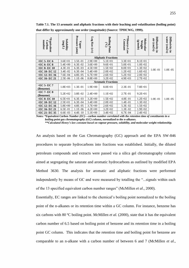
255
Table 7.1. The 13 aromatic and aliphatic fractions with their leaching and volatilisation (boiling point)
that differ by approximately one order (magnitude) (Source: TPHCWG, 1999).
*E
qu
iva
lent
Ca
rbo
n
nu
mb
er
So
lub
ility
(mg
/L)
Va
po
r
Pressu
re (atm
)
Lo
g K
oc (c/c)
Bo
iling
Po
int
(°C)
**
Hen
rys L
aw
Co
nsta
nt
Mo
lecula
r
Weig
ht
(g/m
ole)
Diffu
sivity
in
air (cm
2/s)
Diffu
sivity
in
wa
ter (cm2
/s)
Aliphatic Fractions
>EC 5- EC 6 3.6E+01 3.5E–01 2.9E+00 5.1E+01 3.3E+01 8.1E+01
1.0E–01 1.0E–05
>EC 6- EC 8 5.4E+00 6.3E–02 3.6E+00 9.6E+01 5.0E+01 1.0E+02
>EC 8- EC 10 4.3E–01 6.3E–03 4.5E+00 1.5E+02 8.0E+01 1.3E+02
>EC 10- EC 12 3.4E–02 6.3E–04 5.4E+00 2.0E+02 1.2E+02 1.6E+02
>EC 12- EC 16 7.6E–04 4.8E–05 6.7E+00 2.6E+02 5.2E+02 2.0E+02
>EC 16- EC 21 2.5E–06 1.1E–06 8.8E+00 3.2E+02 4.9E+03 2.7E+02
Aromatic Fractions
>EC 5- EC 7
(Benzene) 1.8E+03 1.3E–01 1.9E+00 8.0E+01 2.3E–01 7.8E+01
1.0E–01 1.0E–05
>EC 7- EC 8
(Benzene) 5.2E+02 3.8E–02 2.4E+00 1.1E+02 2.7E–01 9.2E+01
>EC 8- EC 10 6.5E+01 6.3E–03 3.2E+00 1.5E+02 4.8E–01 1.2E+02
>EC 10- EC 12 2.5E+01 6.3E–04 3.4E+00 2.0E+02 1.4E–01 1.3E+02
>EC 12- EC 16 5.8E+00 4.8E–05 3.7E+00 2.6E+02 5.3E–02 1.5E+02
>EC 16- EC 21 6.5E–01 1.1E–06 4.2E+00 3.2E+02 1.3E–02 1.9E+02
>EC 21- EC 35 6.6E–03 4.4E–10 5.1E+00 3.4E+02 6.7E–04 2.4E+02
Notes: *Equivalent Carbon Number (EC)—carbon number correlated with the retention time of constituents in a
boiling point gas chromatography (GC) column, normalized to the n-alkanes.
**Calculated Henry’s law constant based on vapour pressure, solubility, and molecular weight relationship.
An analysis based on the Gas Chromatography (GC) approach and the EPA SW-846
procedures to separate hydrocarbons into fractions was established. Initially, the diluted
petroleum compounds and extracts were passed via a silica gel chromatography column
aimed at segregating the saturate and aromatic hydrocarbons as outlined by modified EPA
Method 3630. The analysis for aromatic and aliphatic fractions were performed
independently by means of GC and were measured by totalling the “...signals within each
of the 13 specified equivalent carbon number ranges” (McMillen et al., 2000).
Essentially, EC ranges are linked to the chemical‟s boiling point normalized to the boiling
point of the n-alkanes or its retention time within a GC column. For instance, benzene has
six carbons with 80 ºC boiling point. McMillen et al. (2000), state that it has the equivalent
carbon number of 6.5 based on boiling point of benzene and its retention time in a boiling
point GC column. This indicates that the retention time and boiling point for benzene are
comparable to an n-alkane with a carbon number of between 6 and 7 (McMillen et al.,

256
2000). Figure D.7.1 (p.538) of TPHCWG (1998) in Appendix-D indicates the correlation
between ranges of boiling points and the carbon number for a number of typical petroleum
products. It is evident from the figure that there is an overlap between the range of carbon
number for various products and the overlap in equivalent analytical methods.
Based on McMillen et al. (2000), the criteria for toxicity were established for the EC
number fractions by performing a detailed review of literature based on all available
information related to pure compounds, specific petroleum fractions and refined products.
The established toxicity criteria are expressed as oral reference doses (RfD) in mg/kg/day
or as reference concentrations (RfC) in mg/m3 for inhalation exposure based on U.S EPA
as exhibited in Table 7.2. RfD are the expected exposure to human population in one day.
Table 7.2. The TPHCWG Petroleum Fractions (Source: Environment Agency, 2003).
Note: *NA: Not available, ** Based on USEPA benzene value.
The methods in determining TPH RBSLs were set up by integrating the fractionation
scheme, fate and transport properties as well as criteria for toxicity established for the
equivalent carbon number fractions in the ASTM RBCA framework (McMillen et al.,
2000).
The TPHCWG employs risk assessment techniques and assumptions in accordance with
those specified in the ASTM standard. RBSLs were developed by totalling the Hazard
Equivalent Carbon Number Reference Dose (mg/kg bw/d) Reference Concentration
(mg/m3)
TPH-Aliphatic fractions
>EC5- EC6 5.0 18.4
>EC6 - EC8 5.0 18.4
>EC8 - EC10 0.1 1
>EC10 - EC12 0.1 1
>EC12 - EC16 0.1 1
>EC16 - EC21 2.0 *NA
TPH-Aromatic Fractions
>EC5 - EC7 **0.004
**0.03
>EC7 - EC8 0.2 0.4
>EC8 - EC10 0.04 0.2
>EC10 - EC12 0.04 0.2
>EC12 - EC16 0.04 0.2
>EC16 - EC21 0.03 *NA
>EC21 - EC35 0.03 *NA

257
Quotients (HQ) for the 13 corresponding carbon number fractions. For any given fraction,
the HQ refers to the ratio of exposure level of that fraction against a stipulated period of
time to the reference dose allocated to that fraction. The sum of the individual HQ is
referred to as the Hazard Index (HI) (McMillen et al., 2000).
As a general indication, a greater HQ value signifies a higher level of concern (i.e.
potential risk). HQ indices with values higher than unity indicate higher probability of
detrimental health effects (i.e. potential risk); there is a proposal to undertake a additional
detailed investigation or plan for remedial action (RISC-5, 2011). As stated by McMillen
et al. (2000), for each EC number fraction, the HQ was computed by taking the fraction
weight multiplied by the total TPH (mg/kg) and divided by the RBSLs of the fraction. Hua
et al. (2012), claim that the globally suitable non-carcinogenic HQ for the site-specific risk
level is HQ ≤ 1; however the acceptable carcinogenic risk (excess lifetime cancer risk)
differs between countries. For the Netherlands, for instance, it is less stringent at 10-4
as
compared to 10-5
practiced in the UK. The recommendation from the U.S. ASTM standard
is 10-6
and 10-4
for the single pollutant risk target and accumulated contaminants risk
target, respectively, (Hua et al., 2012).
The generic quantitative risk assessment (GQRA) screens risks to human health through
the use of published generic screening values, which have been derived from a set of
conservative assumptions; therefore, the GQRA or a detailed quantitative risk assessment
(DQRA) is generally used to discover risk targets. Human health risks from exposure to
contaminated soil and vapour are also determined by GQRA (PB, 2011). These generic
screening values usually incorporate risk-based Soil Guideline Values (SGVs) or other
Generic Assessment Criteria (GACs) typically based on UK legislation which was in turn
based on the Environment Agency‟s Contaminated Land Exposure Assessment (CLEA)
258
model (see Environment Agency‟s SR2, SR3 and SR7 reports (CL: AIRE, 2014 & PB,
2011).
When there is a plausible pollutant linkage, GQRA is used to compare concentrations of
the contaminants – if remediation is not already planned. The comparisons will be made of
the soil, water and/or soil vapour, which will be assessed for the generic criteria (GAC)
values most appropriate (CL: AIRE, 2014).
The site specific assessment criteria (SSAC) was developed by DQRA; this assessment
includes examining “...each of the exposure pathways and modifying the generic
assumptions” derived from the GACs so that site conditions are thoroughly investigated
(Searl, 2012). In other words, should levels of contaminant be greater than the GAC, or if
generic screening criteria are not applicable to various sites, then DQRA will be used for to
develop SSAC. Additionally, pollutant linkages will be taken into greater account within
DQRA evaluation; consideration regarding remedial options can then be carried out (CL:
AIRE, 2014).
CL: AIRE (2014), recognises that doubt caused by using SGV/GACs within a GQRA is
typically greater than that associated with the use of SSACs within a DQRA. However,
including site-specific information which would take into account details of the exposure
scenario, receptor behaviour, soil type and foundation construction, i.e. the derivations of
the SSAC, permits a more realistic and thus more accurate estimate of risk; in fact, GACs,
are derived from a wider application and more conservative range of sites.
In fact, when a GAC becomes more inclusive, it loses its ability to be applicable to
individual sites and therefore becomes more uncertain.
To conclude, this study evaluated the human health risk through the use of DQRA;
utilising the derivation of the SSAC instead of GQRA allowed more realistic and more
accurate research. This was necessary in light of the fact that the study site (in Kuwait) has

259
a hot and arid climate; the GQRA (as it was derived from GACs values used under cold
climate) is better suited to colder climates such as UK.
7.4 Risk Assessment Stages (RAS)
In performing a risk assessment, a four-stage process approach was developed by the U.S.
National Academy of Sciences which was subsequently adopted by the U.S. EPA (La
Grega et al. 1994). This broadly acceptable approach entails certain processes, namely
Hazard Identification, Exposure Assessment, Toxicity Assessment and Risk
Characterisation. Nathanail et al. (2007) divided risk assessment into two phases with two
sub-phases for each, as listed below:
Phase 1a-Hazard Identification.
Phase 1b-Hazard Assessment.
Phase 2a-Risk Estimation.
Phase 2b- Risk Evaluation.
These risk assessment stages formulated by Nathanail et al. (2007) and the U.S National
Academy of Sciences (La Grega et al., 1994) attained similar targets and objectives in
assessing the risks from contaminated soils from areas affected with hydrocarbon.
Furthermore, the detailed evaluation carried out during the risk assessment process could
form the basis for choosing a suitable regulatory response to a potential environmental risk,
also known as risk management (La Grega et al., 1994). Therefore, for this particular
study, risk assessment scenarios as defined by Nathanail et al. (2007) were implemented.
The soil screening level value with regards to the TPH value at the contaminated site, (dry
oil lake at the Al-Magwa area) for this study, is in accordance with the recommendations
from the Texas State (U.S EPA) which is 100 mg/kg.
260
The reasons the researcher followed the U.S EPA (in particular Texas State) are shown
below:
The Kuwait Environment Public Authority (KEPA) complies with the
U.S EPA standard (ASA, 2012).
The HHRA software (RISC-5) employed in this study is in compliance
with the U.S. EPA standard (RISC-5, 2011).
The Kuwaiti climate is hot and dry, i.e. very similar to that of Texas
State.
The most commonly used value for petroleum clean-up in USA is 100
mg/kg as is the hydrocarbon petroleum clean-up value in Texas State.
(Blaisdell & Smallwood, 1993).
The following four sections provide descriptions of all four phases as an introduction to the
state of the art in risk assessment in accordance with Nathanail et al. (2007).
7.4.1 Hazard Identification (phase 1a)
As defined by Sniffer (2007), Hazard Identification is the process at the initial phase of risk
assessment which requires identification and characterisation of the threats arising from
links to the conditions under consideration. As such, the aim at this preliminary stage is to
identify the likely risks at the study site as stipulated by the following questions:
What are the concerned constituents/pollutants/contaminants, i.e. the
source(s)?
What is the nature of the hazard, i.e. naturally occurring or
anthropogenic (man-made)?
Are there any particular circumstances to be considered such as
leachate and emission in the soil?
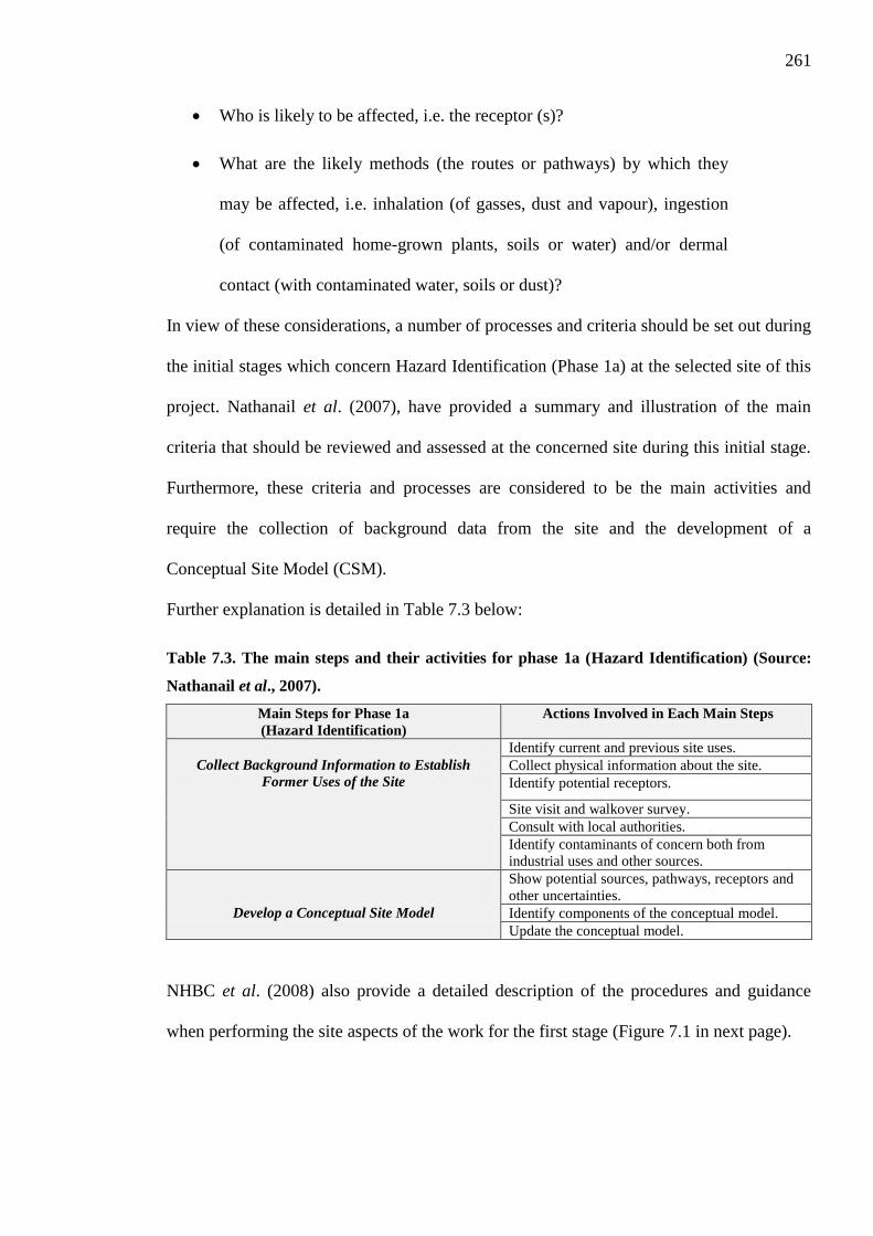
261
Who is likely to be affected, i.e. the receptor (s)?
What are the likely methods (the routes or pathways) by which they
may be affected, i.e. inhalation (of gasses, dust and vapour), ingestion
(of contaminated home-grown plants, soils or water) and/or dermal
contact (with contaminated water, soils or dust)?
In view of these considerations, a number of processes and criteria should be set out during
the initial stages which concern Hazard Identification (Phase 1a) at the selected site of this
project. Nathanail et al. (2007), have provided a summary and illustration of the main
criteria that should be reviewed and assessed at the concerned site during this initial stage.
Furthermore, these criteria and processes are considered to be the main activities and
require the collection of background data from the site and the development of a
Conceptual Site Model (CSM).
Further explanation is detailed in Table 7.3 below:
Table 7.3. The main steps and their activities for phase 1a (Hazard Identification) (Source:
Nathanail et al., 2007).
Main Steps for Phase 1a
(Hazard Identification)
Actions Involved in Each Main Steps
Collect Background Information to Establish
Former Uses of the Site
Identify current and previous site uses.
Collect physical information about the site.
Identify potential receptors.
Site visit and walkover survey.
Consult with local authorities.
Identify contaminants of concern both from
industrial uses and other sources.
Develop a Conceptual Site Model
Show potential sources, pathways, receptors and
other uncertainties.
Identify components of the conceptual model.
Update the conceptual model.
NHBC et al. (2008) also provide a detailed description of the procedures and guidance
when performing the site aspects of the work for the first stage (Figure 7.1 in next page).

262
Figure 7.1. Flowchart for the Hazard Identification (phase 1a) process (Source: NHBC et al.,
2008).
Within this phase of Hazard Identification (1a) of the risk assessment, it is essential to
generate a CSM as one of the processes for the contaminated site. As explained in (LQM,
2012), the HHRA components of the CSM includes a site plan view, cross sections for the
entire site and a network diagram which should consist of sources, pathways and receptors
for the contaminated site. Further details with regards to practical examples of CSM can be
seen from Figures 7.2, 7.3 and 7.4 in next page.

263
Figure 7.2. An example of top view plan for some site as Conceptual Site Model (CSM) part in phase 1a of risk assessment (Source: LQM, 2012).

264
Figure 7.3. An example of cross section for some site as Conceptual Site Model (CSM) part in phase 1a of risk assessment (Source: LQM, 2012).

265
Figure 7.4. An example of network diagram for some site as Conceptual Site Model (CSM) part in phase 1a of risk assessment (Source: LQM,
2012).

266
In order to perform a risk assessment, it is necessary to fully understand the types of
chemicals present, the level of concentration and the way these chemicals travel
(pathways) in the environment of the contaminated area to the potential receptors
(Angehrn, 1998).
It is therefore essential within this study to understand the chemical composition of the
TPH contaminants as well as their level of concentration at the contaminated site in the
Greater Burgan Oil Field (Al- Magwa area). Equally important is to identify the source of
TPH contaminants, pathway routes and the potential receptors. In fact, the Hazard
Identification stage at the contamination site deals with aliphatic and aromatic
hydrocarbons (TPH) including the level of their concentration (mg/kg), the pathway
connections, e.g.: dermal contact, ingestion of the soil and inhalation, and the receptors
affected, e.g. children and adults.
7.4.2 Hazard Assessment (phase 1b)
A review of the site and an appropriate exploratory investigation should be performed
during this stage, so as to carry out phase 1b of the Hazard Assessment at the contaminated
site (dry oil lake). (Nathanail et al., 2007) At this stage, the conceptual model is reviewed
in more detail, so as to ascertain the probability of the presence of any potential
contaminant linkages (Sniffer, 2007).
According to Sniffer (2007), a number of questions should be raised, for example: whether
the exposure is uninterrupted or intermittent; what the spatial scale is, e.g. whether its
effect is localised or more extensive; what the likely period is; the destiny and movement
of the constituents within the environment, i.e. the likelihood of aerial deposition;
discharges to the water environment; reaction within the soil; and how the receptors
behave, e.g. how frequently are they exposed?
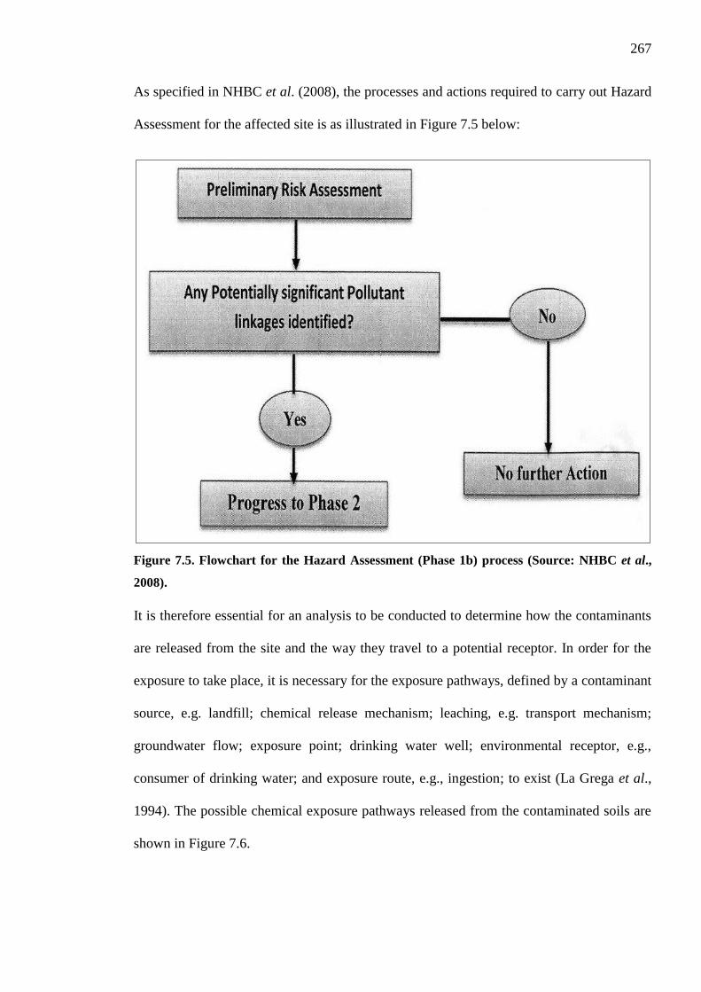
267
As specified in NHBC et al. (2008), the processes and actions required to carry out Hazard
Assessment for the affected site is as illustrated in Figure 7.5 below:
Figure 7.5. Flowchart for the Hazard Assessment (Phase 1b) process (Source: NHBC et al.,
2008).
It is therefore essential for an analysis to be conducted to determine how the contaminants
are released from the site and the way they travel to a potential receptor. In order for the
exposure to take place, it is necessary for the exposure pathways, defined by a contaminant
source, e.g. landfill; chemical release mechanism; leaching, e.g. transport mechanism;
groundwater flow; exposure point; drinking water well; environmental receptor, e.g.,
consumer of drinking water; and exposure route, e.g., ingestion; to exist (La Grega et al.,
1994). The possible chemical exposure pathways released from the contaminated soils are
shown in Figure 7.6.
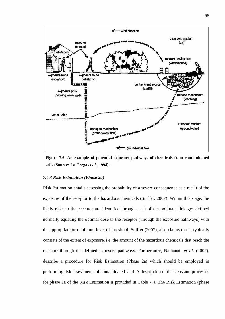
268
Figure 7.6. An example of potential exposure pathways of chemicals from contaminated
soils (Source: La Grega et al., 1994).
7.4.3 Risk Estimation (Phase 2a)
Risk Estimation entails assessing the probability of a severe consequence as a result of the
exposure of the receptor to the hazardous chemicals (Sniffer, 2007). Within this stage, the
likely risks to the receptor are identified through each of the pollutant linkages defined
normally equating the optimal dose to the receptor (through the exposure pathways) with
the appropriate or minimum level of threshold. Sniffer (2007), also claims that it typically
consists of the extent of exposure, i.e. the amount of the hazardous chemicals that reach the
receptor through the defined exposure pathways. Furthermore, Nathanail et al. (2007),
describe a procedure for Risk Estimation (Phase 2a) which should be employed in
performing risk assessments of contaminated land. A description of the steps and processes
for phase 2a of the Risk Estimation is provided in Table 7.4. The Risk Estimation (phase

269
2a) procedures are also detailed by NHBC et al. (2008) as illustrated in the following
Figure 7.7.
Table 7.4. The main steps and their activities for phase 2a (Risk Estimation) (Source:
Nathanail et al., 2007).
Main steps for phase 2a (Risk
Estimation) Actions included in each main step
Design and implement ground
investigation
Design of investigation.
Use of investigation techniques.
Analysis of results.
Consideration of uncertainty.
Evaluation of costs.
Quantitative or qualitative Risk
Estimation
Risk Estimation using guidelines values for
human health.
Derivation of site specific risk assessment
criteria for human health from toxicity data
and likely exposure.
Non-human health assessment criteria
Estimation of short-term exposure.

270
Figure 7.7. Flowchart for the Risk Estimation (phase 2a) process (Source: NHBC et al., 2008).

271
7.4.4 Risk Evaluation (Phase 2b)
According to NHBC et al. (2008), a conceptual phase of risk assessment entails measuring
the adequacy of the estimated risk, considering the nature and magnitude of risk
estimations, any doubts linked to the estimate as well as the general advantages and
disadvantages of taking appropriate action to alleviate such risk.
The aim of performing Risk Evaluation is to appreciate the result of the previous phases
and to decide whether risk management action is required. It is important that the risk
evaluation be performed on a site specific approach taking into account all potential
pollutant linkages. Based upon Sniffer (2007), remedial action may or may not be required
for any given estimate of risk, subject to the legal system under which the assessment is
being performed.
As stated by Nathanial et al. (2007), Risk Evaluation (Phase 2b) is performed by
identifying unacceptable risks and developing provisional risk management objectives.
Additionally, the processes in performing Risk Evaluation (Phase 2b) were described and
specified based on (NHBC et al., 2008) as indicated in Figure 7.8.

272
Figure 7.8. Flowchart for the Risk Evaluation (Phase 2b) process (Source: NHBC et al.,
2008).
7.5 Risk Assessment Stages (RAS) Implementation on the Contaminated Site (Al
Magwa area)
A risk assessment was undertaken for the Al-Magwa site. RICS-5 software was utilised to
determine the concentrations of hydrocarbon contamination with regards to carcinogenic
and non-carcinogenic health effects and their effect on human health as well as to obtain
appropriate clean-up target levels required for any future development.
7.5.1 Hazard Identification (phase 1a)
7.5.1.1 Site Definition and Description
The dry oil lake site located on the Al-Magwa Oil Field is considered one of the three
sectors of the Greater Burgan Oil Field located 20 km away from the densely populated
City of Kuwait. The study site (dry oil lake) is close to Gas centre (GC-09) and several oil
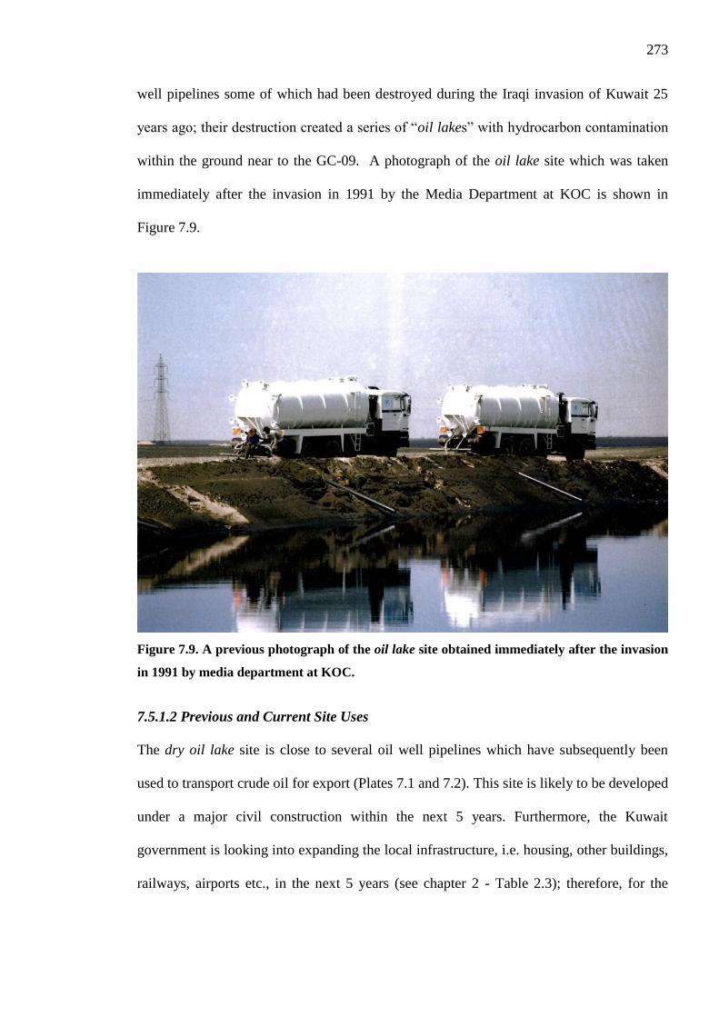
273
well pipelines some of which had been destroyed during the Iraqi invasion of Kuwait 25
years ago; their destruction created a series of “oil lakes” with hydrocarbon contamination
within the ground near to the GC-09. A photograph of the oil lake site which was taken
immediately after the invasion in 1991 by the Media Department at KOC is shown in
Figure 7.9.
Figure 7.9. A previous photograph of the oil lake site obtained immediately after the invasion
in 1991 by media department at KOC.
7.5.1.2 Previous and Current Site Uses
The dry oil lake site is close to several oil well pipelines which have subsequently been
used to transport crude oil for export (Plates 7.1 and 7.2). This site is likely to be developed
under a major civil construction within the next 5 years. Furthermore, the Kuwait
government is looking into expanding the local infrastructure, i.e. housing, other buildings,
railways, airports etc., in the next 5 years (see chapter 2 - Table 2.3); therefore, for the

274
purpose of this study, the site is assumed to be being used for building residential housing.
This will be the scenario adopted for the risk assessment.
Plate 7.1. The oil wells pipelines nearby to the dry oil lake site (Al-Magwa Area).
Plate 7.2. Dry oil lake site (Al-Magwa Area).

275
7.5.1.3 Conceptual Site Model (CSM)
As indicated in Section 4.4.4 of Chapter 4, the data concerning the ground conditions of
the site was obtained from surveys conducted earlier by a construction company (INCO,
2007). The below-ground geological sequence encountered at the Greater Burgan Field site
(Al-Magwa area) are broadly comprised of layers of poorly graded sand (SP) and silty sand
(S-M). Water was discovered during drilling of the boreholes by INCO Lab at 10 m below
ground surface (Figures A.4.12a and A.4.12b).
Al-Sulaimi and Mukhopadhyay (2000), pointed out that the geology of Kuwait is
dominated by rocks from the Tertiary Age dating from the Palaeocene to the Eocene.
Limestones, dolomites and evaporitic profiles (anhydrites) of the Dammam, Rus and Umm
Er Radhuma Formations which are uncomfortably overlain by sandstoness from the
Kuwait Group consisting of the Ghar and Fars Formations, which also lie above the
Dibdibba Formation. According to Hunting Geology and Geophysics (HGG), (1981), the
solid geology of the Greater Burgan site is underlined with the Ghar and Fars Formations
with inter-bedded sands and clays, some sandstones and weak white nodular limestone.
Superficial deposits are composed of primarily Aeolian sands with intermittent gravels
with sands, muds and calcareous sandstones along the shorelines. Furthermore, the main
oil reservoirs are located within the Cretaceous Burgan, Mauddud and Wara Formations of
the Greater Burgan Oil Field.
7.5.1.4 Initial Conceptual Site Model (CSM)
A CSM was used in order to identify all the potential hydrocarbon pollutant linkages in the
dry oil lake site in order to drive the risk assessment process. The physical state of the
hydrocarbon contamination at the dry oil lake site could be classified as either a Volatile
Organic Compound (VOC) or a LNAPL as assumed at the initial CSM. However, the
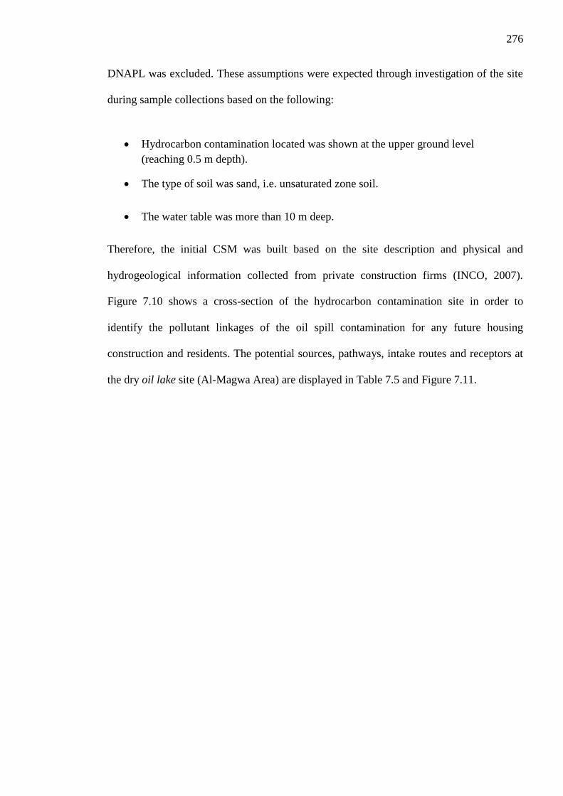
276
DNAPL was excluded. These assumptions were expected through investigation of the site
during sample collections based on the following:
Hydrocarbon contamination located was shown at the upper ground level
(reaching 0.5 m depth).
The type of soil was sand, i.e. unsaturated zone soil.
The water table was more than 10 m deep.
Therefore, the initial CSM was built based on the site description and physical and
hydrogeological information collected from private construction firms (INCO, 2007).
Figure 7.10 shows a cross-section of the hydrocarbon contamination site in order to
identify the pollutant linkages of the oil spill contamination for any future housing
construction and residents. The potential sources, pathways, intake routes and receptors at
the dry oil lake site (Al-Magwa Area) are displayed in Table 7.5 and Figure 7.11.
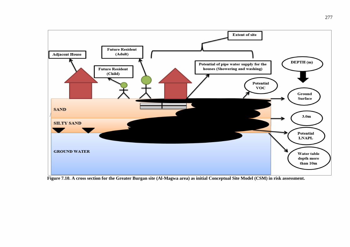
277
Figure 7.10. A cross section for the Greater Burgan site (Al-Magwa area) as initial Conceptual Site Model (CSM) in risk assessment.

278
Table 7.5. The Potential sources, pathways, intake route and receptors in the contamination dry oil lake site (Al-Magwa Area).
Sources Pathways Intake Routes Receptors
Oil Spills
Direct Exposure Dermal contact and soil Ingestion.
Future residents such as child &
Adult Residents on site
Volatilizes hydrocarbon substances, Inhalation indoor air, Inhalation
Outdoor air,
Future residents such as child &
Adult Residents on site
Soil adheres vegetables Ingestion of the vegetables
Future residents such as child &
Adult Residents
Soil Erosion Inhale Particulates air
Future residents such as child &
Adult Residents on site and off site
Leaching to Ground Water and Ground
water transport to Borehole
Ingestion water, Showering Dermal
contact and Showering Vapor in
halation.
Future residents off site such as child
& Adult Residents and drinking
Water Consumer
Ground Water
---------
Marin Ecosystem, Fresh water
Ecosystem
Diffusion through water supply pipes
and air condition
Showering Dermal contact and
Showering Vapor in halation.
On site
Chloride and Sulfate substances ------------- Building Material
279
Figure 7.11. Network diagram for dry oil lake site (Al-Magwa Area) as Conceptual Site Model (CSM) part in phase 1a of risk assessment.

280
7.5.2 Hazard Assessment (phase 1b)
7.5.2.1 Hydrocarbon Contamination Detected in the Site
As mentioned in section (6.5), 110 samples were collected from different depths of (0.0 m,
0.25 m, 0.5 m, 1.0 m, 1.5 m and 2.0 m) 22 samples of which were taken from each of the
above depths. GC-MS tests were conducted on these samples with only 24 samples found
to be polluted with hydrocarbon. The number of samples which were found to be polluted
with hydrocarbon at the site, can be separated related to TPH fractions such as aliphatic
(EC10 to EC35) and aromatic (EC8 to EC35) are as follows:
16 samples from 0.0 m depth.
7 samples from 0.25 m depth.
1 sample from 0.5 m depth.
Furthermore, 7 chemical substances were detected in the soil samples related to
Anthracene and Phenanthrene compounds (which might be toxic because these compounds
are non-volatile and related to PAH).
According to DEFRA (2005), the PAH compounds have proven to be toxic, human
carcinogens; they are the results of incomplete carbon combustion from fuels containing
carbon. PAH are the results of two (or more) aromatic (benzene) rings; these may fuse
together when a carbon pair atoms is shared between them. Naphthalene and
benzo(a)pyrene, for example, are compounds which have been formed by fusing together 2
(naphthalene) and 5 (benzo(a)pyrene) rings which have fused (BC, n.d.), Chemical and
physical characteristics of the above compounds related to PAH vary in molecular weight.
In fact, with increases of vaporisation their weight of molecular is increased; however,
their solubility of aqueous decreases. Additionally, their behaviour, distribution in the
environment, and their effects on biological systems are different. Lower weight of
molecular, i.e. 2 to 3 ring groups, for example, naphthalenes - are particularly toxic for
281
aquatic organisms, but PAH with higher weight of molecular, i.e. 4 to 7 rings for example
benzo(a)pyrene are not although several members of the high molecular weight PAHs have
been known to be carcinogenic (BC, n.d.).
The PAH referred to above were taken into consideration during investigation at the
contamination site; however, the GC-MS testing instrument did not identify them during
the contaminated soil sample testing. This could be attributed to the following reasons:
The behaviour of Naphthalene chemical substances, according to DEFRA (2005),
degrades extensively in soil under aerobic and anaerobic conditions. It could,
therefore, be considered to have been degraded at the study site (Al-Magwa area)
since it had been there for more than 23 years.
The behaviour of Benzo(a)pyrene chemical substances is regarded to have
evaporated hugely (BC, n.d.); it could have evaporated at the site since the climate
in the area is particularly hot and arid and the conditions have existed for more than
two decades.
Various unknown GC-MS peak (not identified by the Kuwait diesel standard used during
calibration as standard and might not be hydrocarbon concentrations) were found in some
soil samples by the GC-MS test at depths of 0.0 m and 0.25 m. All the concentrations
(mg/kg) of these varied hydrocarbons found in the dry oil lake are displayed in Table 7.6.
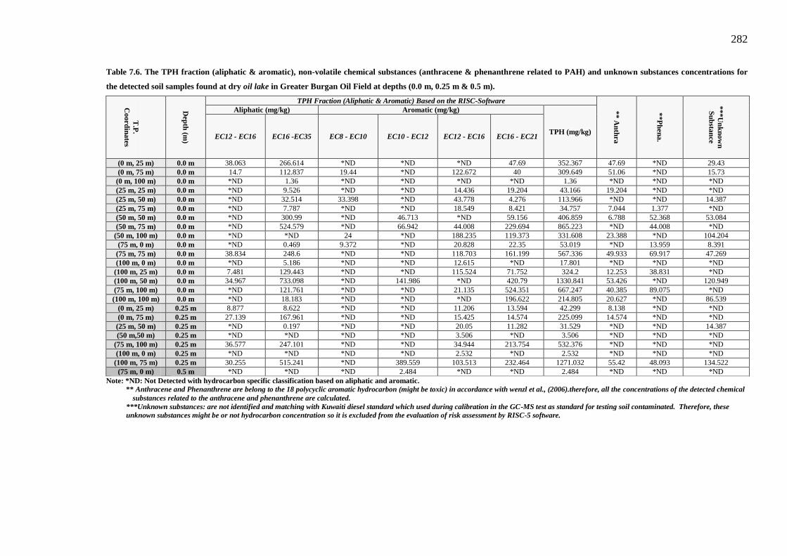
282
Table 7.6. The TPH fraction (aliphatic & aromatic), non-volatile chemical substances (anthracene & phenanthrene related to PAH) and unknown substances concentrations for
the detected soil samples found at dry oil lake in Greater Burgan Oil Field at depths (0.0 m, 0.25 m & 0.5 m).
T.P
.
Co
ord
ina
tes
Dep
th (m
)
TPH Fraction (Aliphatic & Aromatic) Based on the RISC-Software
** A
nth
ra
**P
hen
a.
***
Un
kn
ow
n
Su
bsta
nce
Aliphatic (mg/kg) Aromatic (mg/kg)
TPH (mg/kg) EC12 - EC16 EC16 -EC35 EC8 - EC10 EC10 - EC12 EC12 - EC16 EC16 - EC21
(0 m, 25 m) 0.0 m 38.063 266.614 *ND *ND *ND 47.69 352.367 47.69 *ND 29.43
(0 m, 75 m) 0.0 m 14.7 112.837 19.44 *ND 122.672 40 309.649 51.06 *ND 15.73
(0 m, 100 m) 0.0 m *ND 1.36 *ND *ND *ND *ND 1.36 *ND *ND *ND
(25 m, 25 m) 0.0 m *ND 9.526 *ND *ND 14.436 19.204 43.166 19.204 *ND *ND
(25 m, 50 m) 0.0 m *ND 32.514 33.398 *ND 43.778 4.276 113.966 *ND *ND 14.387
(25 m, 75 m) 0.0 m *ND 7.787 *ND *ND 18.549 8.421 34.757 7.044 1.377 *ND
(50 m, 50 m) 0.0 m *ND 300.99 *ND 46.713 *ND 59.156 406.859 6.788 52.368 53.084
(50 m, 75 m) 0.0 m *ND 524.579 *ND 66.942 44.008 229.694 865.223 *ND 44.008 *ND
(50 m, 100 m) 0.0 m *ND *ND 24 *ND 188.235 119.373 331.608 23.388 *ND 104.204
(75 m, 0 m) 0.0 m *ND 0.469 9.372 *ND 20.828 22.35 53.019 *ND 13.959 8.391
(75 m, 75 m) 0.0 m 38.834 248.6 *ND *ND 118.703 161.199 567.336 49.933 69.917 47.269
(100 m, 0 m) 0.0 m *ND 5.186 *ND *ND 12.615 *ND 17.801 *ND *ND *ND
(100 m, 25 m) 0.0 m 7.481 129.443 *ND *ND 115.524 71.752 324.2 12.253 38.831 *ND
(100 m, 50 m) 0.0 m 34.967 733.098 *ND 141.986 *ND 420.79 1330.841 53.426 *ND 120.949
(75 m, 100 m) 0.0 m *ND 121.761 *ND *ND 21.135 524.351 667.247 40.385 89.075 *ND
(100 m, 100 m) 0.0 m *ND 18.183 *ND *ND *ND 196.622 214.805 20.627 *ND 86.539
(0 m, 25 m) 0.25 m 8.877 8.622 *ND *ND 11.206 13.594 42.299 8.138 *ND *ND
(0 m, 75 m) 0.25 m 27.139 167.961 *ND *ND 15.425 14.574 225.099 14.574 *ND *ND
(25 m, 50 m) 0.25 m *ND 0.197 *ND *ND 20.05 11.282 31.529 *ND *ND 14.387
(50 m,50 m) 0.25 m *ND *ND *ND *ND 3.506 *ND 3.506 *ND *ND *ND
(75 m, 100 m) 0.25 m 36.577 247.101 *ND *ND 34.944 213.754 532.376 *ND *ND *ND
(100 m, 0 m) 0.25 m *ND *ND *ND *ND 2.532 *ND 2.532 *ND *ND *ND
(100 m, 75 m) 0.25 m 30.255 515.241 *ND 389.559 103.513 232.464 1271.032 55.42 48.093 134.522
(75 m, 0 m) 0.5 m *ND *ND *ND 2.484 *ND *ND 2.484 *ND *ND *ND
Note: *ND: Not Detected with hydrocarbon specific classification based on aliphatic and aromatic.
** Anthracene and Phenanthrene are belong to the 18 polycyclic aromatic hydrocarbon (might be toxic) in accordance with wenzl et al., (2006).therefore, all the concentrations of the detected chemical
substances related to the anthracene and phenanthrene are calculated.
***Unknown substances: are not identified and matching with Kuwaiti diesel standard which used during calibration in the GC-MS test as standard for testing soil contaminated. Therefore, these
unknown substances might be or not hydrocarbon concentration so it is excluded from the evaluation of risk assessment by RISC-5 software.

283
ProUCL Statistics Software for the Quantitative data
As mentioned by Barnett et al. (2013), USEPA has funded the development of ProUCL 5.0
software in an effort to instigate rigorous and defensible statistics so as to assist the
decision makers allowing them to arrive at correct decisions at contaminated sites in order
to help and protect human health as well as the environment.
For data sets with and without non-detect (ND) considerations, the statistics were
calculated by ProUCL by means of parametric and non-parametric techniques
encompassing a wide-range of data skewness, data distributions and sizes of samples
(Barnett et al., 2013).
According to Barnett et al. (2013), non-parametric methods were devised so as be used
when the researcher has no knowledge of the existing parameters, i.e. has no assumptions
regarding the variables of interests that the population may have. In other words,
assessment of parameters is not reliant upon non-parametric methods.
This software can calculate the Upper Confidence Limits (95 % - UCLs of the mean)
which can correct any skewed data. Explanatory graphical methods for uncensored data
sets as well as left-censored data sets comprising non-detect (ND) observations are
available in the ProUCL (Barnett et al. 2013). This software includes graphical methods
consisting of histograms, multiple quantile-quantile (Q-Q) plots, and side-by-side box
plots. Graphic displays help to provide additional understanding of the information
contained in a data set which may not otherwise be shown by utilising estimates, e.g. 95 %
upper limits in term of whether the sample sets are normal distribution or non-normal
distribution (Barnett et al. 2013).

284
The non-parametric method for the 95 % - UCLs of the mean (via ProUCL software)
might be used for concentrations of the detected hydrocarbon contamination at the site in
order to establish confident answers and a correct decision on the samples concentrations.
Thus, the normality of the data was then examined using the Shapiro Wilk Test of
Normality after outliers were deleted from the dataset. The data followed the non-normal
distributions which is considered acceptable for performing non-parametric statistical tests
(95 % UCLs of the mean) to detect TPH concentrations fraction (aliphatic and aromatic)
and chemical substances related to Anthracene and Phenanthrene compounds at depths of
0.0 m, 0.25 m and 0.5 m (Figures D.7.2 to D.7.9).
One example of a Q-Q plot for the detected aliphatic (EC12 - EC16) concentrations found
in soil contaminated with TPH shows non-normal distribution as displayed in Figure 7.12.
Therefore, the 95 % UCL of mean (mg/kg), of the detected hydrocarbon contamination of
concern (as mentioned above), are shown in Table 7.7. The minimum/maximum, mean and
standard deviation values are also recorded in this Table. (Figures D.7.10 to D.7.18 at
Appendix-D).
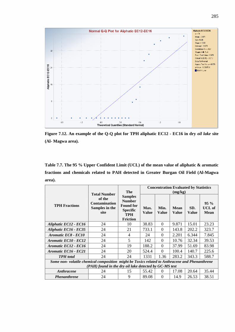
285
Figure 7.12. An example of the Q-Q plot for TPH aliphatic EC12 - EC16 in dry oil lake site
(Al- Magwa area).
Table 7.7. The 95 % Upper Confident Limit (UCL) of the mean value of aliphatic & aromatic
fractions and chemicals related to PAH detected in Greater Burgan Oil Field (Al-Magwa
area).
TPH Fractions
Total Number
of the
Contamination
Samples in the
site
The
Samples
Number
Found for
Specific
TPH
Friction
Concentration Evaluated by Statistics
(mg/kg)
Max.
Value
Min.
Value
Mean
Value
SD.
Value
95 %
UCL of
Mean
Aliphatic EC12 - EC16 24 10 38.83 0 9.871 15.01 23.23
Aliphatic EC16 - EC35 24 21 733.1 0 143.8 202.2 323.7
Aromatic EC8 - EC10 24 4 24 0 2.201 6.344 7.845
Aromatic EC10 - EC12 24 5 142 0 10.76 32.34 39.53
Aromatic EC12 - EC16 24 19 188.2 0 37.99 51.69 83.98
Aromatic EC16 - EC21 24 20 524.4 0 100.4 140.7 225.6
TPH total 24 24 1331 1.36 283.2 343.3 588.7 Some non- volatile chemical composition might be Toxics related to Anthracene and Phenanthrene
(PAH) found in the dry oil lake detected by GC-MS test
Anthracene 24 15 55.42 0 17.08 20.64 35.44
Phenanthrene 24 9 89.08 0 14.9 26.53 38.51

286
7.5.2.2 Hydrocarbon Contamination Exceed Screening Value
This study has adopted the most common figure for the clean-up level values used in
Texas State (U.S) which is 100 mg/kg for TPH as recommended by Blaisdell and
Smallwood (1993) to determine whether or not a risk assessment is required for a clean-up
of the contaminated site (Al-Magwa area). The result for the Al-Magwa site shows that the
95 % upper confidence limit (UCL) of mean value of the total TPH concentration
contaminated with soil is 588.7 mg/kg which is well above the screening value for Texas
State of 100 mg/kg. This indicates that an urgent risk assessment is required for this site; in
carrying out this risk assessment, 95 % UCL concentrations of the mean values of the TPH
fractions (aliphatic and aromatic) and the chemicals discovered connected to Anthracene
and Phnanthrene (PAH) were employed in the RISC-5 modelling (Table 7.8 below and
Figures D.7.19 & D.7.20 Appendix-D).
Table 7.8. Comparison between the mean value of 95 % UCL of the of TPH concentration (mg/kg) in
the site and the approved Screening Value in the soil by U.S. EPA.
Mean values of 95% UCL of
TPH Concentration in the
Soil at Greater Burgan Oil
Field (Al-Magwa Area)
Screening Value in the Soil
by Texas State (Blaisdell &
Smallwood, 1993)
Comments
588.7 mg/kg 100 mg/kg
It needs to evaluate the
human health risk assessment
by using RISC-5 software.
7.5.2.3 Final Conceptual Site Model (CSM)
After identifying the hydrocarbon contamination depth and concentrations by GC-MS
results, it was found that the TPH concentration in the soil exceeds the screening value.
CSM has been updated and reviewed; the final cross-section diagram of the contaminated
site is shown in Figure 7.13. The potential sources, pathways, intake routes and receptors at
the dry oil lake site (Al-Magwa area) are as displayed in Table 7.9 and Figure 7.14.

287
Figure 7.13. A cross section for the Greater Burgan site (al-Magwa area) as Final Conceptual Site Model (CSM) in risk assessment.
288
Table 7.9. Final potential sources, pathways, intake route and receptors in the contamination dry oil lake site (Al-Magwa area).
Sources Pathways Intake Routes Receptors Comments
Continue Yes/No
*Aliphatic EC12 - EC16
*Aromatic EC8 - EC10
*Aromatic EC10 - EC12
*Aromatic EC12 - EC16
Volatilizes
hydrocarbon
substances
Inhalation
Outdoor air
Future residents such as
child & Adult Residents
on site
Most of the contaminated samples were taken from the top soil (0.0 m depth).
Also, the concentration of the oil contamination was over the U.S EPA standard
which is 100 ppm.
yes
Soil Erosion Inhale
Particulates air
Future residents such as
child & Adult Residents
on site and off site
The soil condition was loose and sandy. Moreover, Kuwait has long summer
session rather than the winter which has got strong windy in the summer. These
reasons let the contamination soil (top soil) can move by wind to the adjacent
area.
yes
Leaching to
Ground Water
and Ground
water transport to
Borehole
Ingestion
water,
Showering
Dermal contact
and Showering
Vapor in
halation.
Future residents off site
such as child & Adult
Residents and drinking
Water Consumer
The type of the contaminant is dry and exists since 25 years. Also it is very
seldom rains in Kuwait which could not migrate the contaminants downwards
into the groundwater.
No
Ground Water
----------
Marin Ecosystem, Fresh
water Ecosystem
The depth of the oil contaminated reached 0.5m at the site with only found one
detected soil sample. Moreover, the water table depth is more than 10 m (as
mentioned in section 4.4.4 in chapter 4).
No
Diffusion
through water
supply pipes and
air condition
Showering
Dermal contact,
Showering
Vapor
inhalation and
inhalation from
air condition
On site
As Johnson and Ettinger in 1991 recommend using vapor intrusion model for
houses when the contamination presence underneath the foundation because
they assumed the vapor of the contamination will migrate inside the house from
the foundation pile (EQM, 2004). On the other hand, the soil contamination was
observed in the top of the ground (0.0 m, 0.25 m & 0.5 m) and the foundation
depth is reached 1.0m (in the same zone of the contamination) which let the
builder to remove the hydrocarbon contamination during excavation in order to
build house.
No
*Aliphatic EC16 - EC35
*Aromatic EC16 – EC21
Direct Exposure
Dermal contact
and soil
Ingestion.
Future residents such as
child & Adult Residents
on site
The soil contamination with oil spills at the top soil (0.0 m depth) was observed
and over the U.S EPA standard which is 100 ppm. yes
Soil adheres
vegetables
Ingestion of the
vegetables
Future residents such as
child & Adult Residents
Most of the residents in Kuwait planting some vegetables such a tomato, potato,
carrot and lettuce which their roots small in the ground and do not exceed more
than 0.25m depth (at contamination zone).
yes
*Aliphatic EC12 to EC35
*Aromatic EC8 to EC21
Chloride and
Sulphates
substances
------------- Building Material The Foundation for the house will start with depth 1.0 m moreover, the
contamination only reached from zero to depth 0.5 m.
No
Note: * all the TPH fractions were divided into the relevant pathways as such, the behaviour of the TPH fractions are differ in the environment (i.e. soluble, volatilisation etc. ) (CCME,
2008).

289
Figure 7.14. A network diagram for Greater Burgan oil site (Al-Magwa area) as Final Conceptual Site Model (CSM) in risk assessment.

290
7.5.3 Risk Estimation (phase 2a)
7.5.3.1 Routes Assessed Based on Final CSM and Parameters of the Site Specific and
Contaminants of Concern
Based on the final CSM from the previous stage (see section 7.5.2, Hazard Assessment-
Phase 1b), one hydrocarbon contaminated pathway was evaluated in the RICS-5 modelling
using fate and transport techniques; for example, the unsaturated zone soil pathway with
the assumption of different routes. These pathways are: Soil Ingestion; Dermal Contact;
and Ingestion of Home-Grown Vegetables; i.e. transport routes through direct contact. This
also includes Inhalation of Outdoor Air (from volatiles) and Particulates Air pathways
which are transported via the contaminants volatilization from the affected soil to ambient
air in the site as well as the spread of small particles of superficially affected soil during
the dust season into adjacent areas (Table 7.10).
The values for the site specific parameters assumed in estimating the exposure point
concentration of the contaminated site, for instance, the outdoor air model, particulate
parameters, source geometry, unsaturated zone, and unsaturated zone lens, are exhibited in
Table 7.11. These values for the site specific parameter employed were based on the
chosen pathway, namely unsaturated zone soil; however, the exception was that of
Kuwait‟s average wind speed (m/s) for the outdoor air model and particulates of
parameters which were obtained in accordance with Al-Ajmi (1994). Other parameters
used were the default values recognised by the RISC-5 software as used by the U.S EPA.
In addition, the values of the source geometry were used based on the site investigation for
the dry oil lake.
Table 7.12 shows the chemical properties and toxicity figures of the aliphatic fraction
(EC12 to EC35), aromatic fraction (EC8 to EC21) and the chemical substances associated
with Anthracene and Phenanthrene compounds (PAH). These chemical properties and
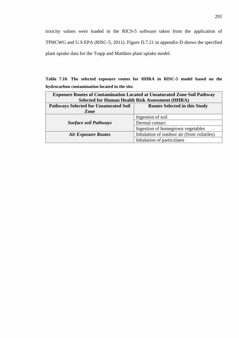
291
toxicity values were loaded in the RICS-5 software taken from the application of
TPHCWG and U.S EPA (RISC-5, 2011). Figure D.7.21 in appendix-D shows the specified
plant uptake data for the Trapp and Matthies plant uptake model.
Table 7.10. The selected exposure routes for HHRA in RISC-5 model based on the
hydrocarbon contamination located in the site.
Exposure Routes of Contamination Located at Unsaturated Zone Soil Pathway
Selected for Human Health Risk Assessment (HHRA)
Pathways Selected for Unsaturated Soil
Zone
Routes Selected in this Study
Surface soil Pathways
Ingestion of soil
Dermal contact
Ingestion of homegrown vegetables
Air Exposure Routes Inhalation of outdoor air (from volatiles)
Inhalation of particulates

292
Table 7.11. Site specific parameters data measured and information of the assumed pathway.
Input parameter based on unsaturated zone soil pathway selected in RISC-5 modeling.
a. Box Data for Outdoor Air
Model Parameters
b. Particulates Parameters (defaults values
suggested in the RISC-5 software) c. Source Geometry Parameters d. Unsaturated Zone Parameters
Non-soil-specific
parameter
Input
Value Non-soil-Specific parameters
Input
Value
Non-Soil-Specific
parameters Input
Value
Parameters with defaults values
available from sand parameters
database: Input Value
Height of Box* 2 m Particulate emission rate (sub
10 micron)* 6.9 E-14
Depth to top of
contamination (may be
zero)****
0 m a.Total porosity*
0.375 cm3/cm3
Width of Box* 10 m Fraction of site with building
or vegetation* 0 Length of source area**** 100 m b. Residual water content*
0.053 cm3/cm3
Length of Box* 10 m Equivalent threshold value of
wind speed at 7m* 11.32 m/s Width of Source area**** 100 m c. Fraction organic carbon*
0.002 goc/gsoil
Wind speed***
4.8
m/s
(*1) Mean annual wind speed
(Um)* 6.16 m/s
Thickness of
contamination**** 0.5 m d. soil bulk density**
1.68 g/cm3
Wind speed distribution
function (F(X))* 0.194
Distance from bottom of
source to groundwater**** 10 m
e. saturated conductivity of the
vadose zone*
6.4 m/d
f. Value of Van Genuchten N* 2.68
g. Thickness of lens* 2.0m
Note:*: it means all the these defaults values suggested by U.S EPA in the RISC-5 software which are used as assumption in this study site in Kuwait because there is no accredited
values related to these parameter approved by Kuwait government or found in literature.
**: it used the sandy soil bulk density of Burgan Oil Field in Kuwait as parameter value (Al-Sarawi et al., 1998b).
***: it used the average wind speed in Kuwait as parameter value (Al-Ajmi, 1994).
****: it used the parameters values as assumption related to the site investigation for the dry oil lake site in Kuwait (Al-Magwa area).

293
Table 7.12. The properties of the chemical substances of concern as assumed in RISC-5 software for contaminated located at unsaturated zone soil
pathway.
Chemical Name
Estimated Properties
Molecular
weight
(g/mol)
Solubility
(mg/L)
Henry’s law
constant
(no NDs)
Koc (ND for
inorganics)
(ml/g)
Kd (soil
partition
coeff.)
(ml/g)
***Log Kow
—
octanol/water
partition
coeff. (L/kg)
Diffusion
coefficient
in air
(cm2/s)
Diffusion
coefficient
in water
(cm2/s)
Reference
concentra
tion (RfC)
mg/m3
Unit
risk
factor
µg/m3
Anthracene 178.2 0.0434 0.00267 29500 *ND 4.55 0.0324 7.74E-06 *ND
*N
D
Phenanthrene 178.2 1.15 0.00148 22900 *ND 4.46 0.0517 5.9E-06 *ND
Aliphatic EC12 - EC16 200 0.00076 540 5010000 *ND 6.84 0.1 1E-05 1
Aliphatic EC16 - EC35 270 1.3E-06 6400 1000000000 *ND 8.91 0.1 1E-05 **NA
Aromatic EC8 - EC10 120 65 0.49 1580 *ND 3.14 0.1 1E-05 0.2
Aromatic EC10 - EC12 130 25 0.14 2510 *ND 3.45 0.1 1E-05 0.2
Aromatic EC12 - EC16 150 5.8 0.054 5010 *ND 3.93 0.1 1E-05 0.2
Aromatic EC16 - EC21 190 0.51 0.013 15800 *ND 4.72 0.1 1E-05 **NA

294
Table 7.12. Continued.
Chemical Name
Estimated Properties
Reference dose
(RfD) oral mg/kg-d
Gastro-intestinal
absorption factor
(dimensionless)
Absorption
adjustment factor:
dermal-soil
(dimensionless)
Uptake factor for
plants (L/kg)
Slope factor oral
1/(mg/kg-d)
Anthracene 0.3 1 0.13
***
Use
Kow
*N
D
phenanthrene *ND 1 0.1
Aliphatic EC12 - EC16 0.1 1 1
Aliphatic EC16 - EC35 2 1 1
Aromatic EC8 - EC10 0.04 1 1
Aromatic EC10 - EC12 0.04 1 1
Aromatic EC12 - EC16 0.04 1 1
Aromatic EC16 - EC21 0.03 1 1 Note: *ND: It means not detected with Petrol.
**NA: It means not available.
***Use Kow: The RISC-5 software recommended to use Kow values.
295
7.5.3.2 Future Resident Receptor Parameters (Child and Adult)
For this present study, children (both male and female) and adults (both male and female)
are considered to be the potential receptors (future residents) to be evaluated for risk
assessment. Risk Evaluation on the receptors (children and adults) was assumed to be
upper percentile exposure defaults as for the “Reasonable Maximum Exposure” (RME).
To evaluate the risks (carcinogenic and non-carcinogenic) on human health of the receptors
from the studied site, the exposure parameter factors used were the default values as
recognised in the RISC-5 model. For instance, the average exposure time for carcinogenic
parameters for both receptors (child and adult) is 70 years. On the other hand, residential
children‟s time outdoors (hours/days) parameter was taken as an assumption of a 12 hour
day rather than a 24 hour day. This was due to the 12 hours spent by child receptors
between sleeping time and school time; the remaining 12 hours were taken to be spent in
the garden. Table 7.13 below tabulates all the exposure parameter values for upcoming
residents.
Contaminant Intake Rate
This present study shows the impact of carcinogenic and non-carcinogenic risks to human
health as related to ingestion of soil, dermal contact, ingestion of home grown vegetables,
inhalation of outdoor air and inhalation of particulates to aliphatic (EC12 to EC35); also
aromatic (EC8 to EC21) fractions in the shallow ground were assessed and calculated. The
risk calculation was performed in accordance with RISC-5 (2011) to ascertain the
estimated rate of intake for each chemical concerned from each exposure route. This Intake
Rate, commonly known as a Dose, is expressed in milligrams per day of chemicals
absorbed into the body per unit of body weight (mg/kg-d). As mentioned in the RISC-5
(2011), the EPA's Risk Assessment Guidance for Superfund (RAGS) Manual (EPA,
1989a) suggests that within the evaluation of longer-term exposure to non-carcinogenic
296
toxicants, the intake should be computed by averaging the intake over the exposure period
(or averaging time). The final result is termed as Chronic Average Daily Dose (CADD)
and is employed in determining the HQ from each route as estimated in the studied area by
comparing against a safe Reference Dose (RfD). In other words, the HQ is equivalent to
the Chronic Average Daily Dose (CADD) for each route estimated at the studied site
divided by the Reference Dose (RfD) of that particular chemical. For carcinogenic risks
computed, the Lifetime Averaged Daily Dose (LADD) was employed in estimating the
Incremental Excess Lifetime Cancer Risk (IELCR) by multiplying the LADD with a
toxicity factor (Slope Factor (SF)). This means that the slope factors are used to measure
potential human carcinogenic risks. A slope factor is an upper-bound lifetime probability
which assumes that exposure to any quantity of a carcinogen will potentially raise the risk
of cancer. The confidence limit of a slope factor is approximately 95 %. The rise in the risk
of cancer is usually expressed in units of proportional influenced per mg of substance/kg
bodyweight-day. This potential human carcinogenic risk is normally kept for use in the
„low-dose area‟ of the „dose- response‟ relationship for exposure corresponding to a risk of
less than 1 in 100. A slope factor should reflect the pathway of intake, e.g., inhalation,
ingestion, or dermal absorption. Unfortunately, toxicological data is not always shown for
each pathway, therefore, pathway-to-pathway extrapolations must be completed (U.S.
EPA, 2016; RISC-5, 2011).
As such, the intake rate of aliphatic and aromatic fraction and chemicals linked to
Anthracene and Phenanthrene (PAH) from the above mentioned assumed pathways in the
area of study were computed by means of specific equations which are displayed in Tables
D.7.3 to D.7.11 of Appendix-D.
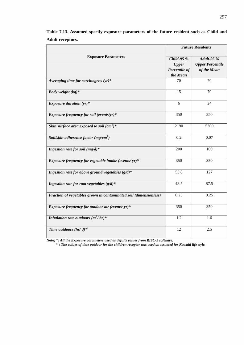
297
Table 7.13. Assumed specify exposure parameters of the future resident such as Child and
Adult receptors.
Exposure Parameters
Future Residents
Child-95 %
Upper
Percentile of
the Mean
Adult-95 %
Upper Percentile
of the Mean
Averaging time for carcinogens (yr)* 70 70
Body weight (kg)* 15 70
Exposure duration (yr)* 6 24
Exposure frequency for soil (events/yr)* 350 350
Skin surface area exposed to soil (cm2)* 2190 5300
Soil/skin adherence factor (mg/cm2) 0.2 0.07
Ingestion rate for soil (mg/d)* 200 100
Exposure frequency for vegetable intake (events/ yr)* 350 350
Ingestion rate for above ground vegetables (g/d)* 55.8 127
Ingestion rate for root vegetables (g/d)* 48.5 87.5
Fraction of vegetables grown in contaminated soil (dimensionless) 0.25 0.25
Exposure frequency for outdoor air (events/ yr)* 350 350
Inhalation rate outdoors (m3/ hr)* 1.2 1.6
Time outdoors (hr/ d)*1 12 2.5
Note; *: All the Exposure parameters used as defults values from RISC-5 software.
*1: The values of time outdoor for the children receptor was used as assumed for Kuwaiti life style.

298
7.5.4 Risk Evaluation (phase 2b)
7.5.4.1 Human Health Carcinogenic Risks
As revealed from the cancer risk values by the RICS-5 software and exhibited in tables
D.7.3 to D.7.11 of Appendix D, the human health (child and adult) cumulative cancer risk
caused by hydrocarbon contamination from sources such as TPH fractions (aliphatic and
aromatic) and the detected chemicals associated with Anthracene and Phenanathrene
(belonging to PAH) from the exposure into the above assumed pathways were concluded
as Not Detected (ND).
7.5.4.2 Human Health Non- Carcinogenic Risks
The effects of the non-carcinogenic risks on human health caused by the Anthracene and
Phenanathrene (PAH) and TPH fraction (aliphatic and aromatic) contamination through the
same above assumed pathways at the site under consideration, are shown in Tables (7.14
and 7.15) and Figures (7.15 and 7.16). These Tables and Figures, show that the total HQ
were 2.7 for children and 1.03 for adults. In other words, HQ was > 1 which means a
potential risk.
7.5.4.3 Site Specific Clean-up Level
The Site Specific Target Level (SSTLs) was calculated from the assumed parameters
(related to the dry oil lake site) which entered into the modelling software as shown in
Tables (7.10) and (7.11).
The outcome of the Site-Specific Target Levels (SSTLs) was obtained from the RISC-5
software by using the individual constituent levels option, i.e. for each contaminated
hydrocarbon substance of concern; and each cumulative risk selection, i.e. risks are added
for all related TPH fractions. The risks‟ clean-up level exposed to the hydrocarbon
contamination in the soil via the assumed pathways at the dry oil lake site (Al-Magwa
area) are demonstrated in Table 7.16.
299
The entire simulation process, including the results obtained from the modelling (RICS-5),
are as indicated in figures D.7.22 to D.7.37 and Tables D.7.12 to D.7.19 in appendix D.
The following table 7.16 demonstrates that the site specific target levels (SSTLs - clean up
levels) values were compared with the concentration of hydrocarbon soil contaminants
discovered at the site under study. The findings clearly demonstrate that the hydrocarbon
contamination concentrations, i.e Anthracene, Phenanthrene, aliphatic (EC12 - EC16),
aliphatic (EC16 - EC35), aromatic (EC8 - EC10), aromatic (EC10 - EC12), aromatic
(EC12 - EC16) and aromatic (EC21 - EC35) are below the SSTLs. However, the tested
concentrations of the aromatic (EC16 - EC21) hydrocarbon are 2.48 times greater than the
calculated SSTLs for these specific hydrocarbons. Additionally, the total of TPH
concentration of the site is higher than the value of SSTLs with a different value of 295.9
mg/kg.
The results from the health risk assessment performed in the area of study are generally
consistent with a similar exercise undertaken by Pinedo et al. (2012) who carried out
research which included undertaking site specific risk assessment for TPH fractions
distribution and concentration utilising the RBCA framework. Two contamination routes
were investigated; each route considered one distinct pathway, for example Volatilization
and Particulates to Outdoor Air Inhalation (through ambient air volatilization of
contaminants from affected soils and small particles of superficial affected soil) and
Surface Soil (through direct ingestion, dermal contact and inhalation).
They found that the Outdoor Air pathway has a lower risk, as shown in the HQ values (HQ
– 0 m = 0.863, HQ – 50 m = 0.42 and HQ – 100 m = 0.138), which are lower than the
upper limit of 1.0. However, the soil risks for each fraction are also less than the HQ limit
and the cumulative risk is above the limit by nearly 1.6. This cumulative risk is primarily
attributed to the aromatic EC16 - EC21 fraction, which accounts for nearly half of the total

300
risk. The total TPH is found only in superficial soil, with a value equivalent of 1.6 times
greater than the Site-Specific Target Levels (SSTLs). Further, Study by Hua et al. (2012) -
whose work also revolved around health risk assessments as a result of exposure to organic
contaminated soil at an oil refinery.
They found that the concentration of benzene, benzo(a)pyrene and benzo(a)anthracene
within the soil obtained from the site were higher than their respective risk screening
values, with the pollutants mainly concentrated within 0.1 to 5.5 m below the ground
surface. They considered three major exposure pathways, namely oral digestion, skin
contact and air inhalation. Their results showed that the three major pathways were capable
of indicating carcinogenic risk (CR) and non-carcinogenic HQ of the contaminated soil
reaching 9.59×10⁻⁵
and 15.46, respectively; these were significantly higher than the
acceptable threshold values of 10-5
and 1.
As with the above study, Pinedo et al. (2012) showed that the HQ value of the Outdoor Air
pathway through exposure to the TPH fraction contamination was lower than the upper
limit of 1.0. However, the cumulative risk (total HQ) was an unacceptable risk value (HQ
> 1) (Pinedo et al., 2012). These values are in line with the findings of the HQ through the
only outdoor air pathway of the current study. On the other hand, the HQ value of
ingestion of vegetables for adults and child receptors was more than 1 (potential risk > 1)
for the current study. Additionally, total HQ values were found to be higher than 1 which is
similar to the current study. All total TPH values for both previous studies (Pinedo et al.,
2012 and the current study) were found to be greater than the SSTLs.
On the other hand, the study by Hua et al. (2012) found that the carcinogenic risk (CR)
value of contaminated soil (benzene, benzo(a)pyrene and benzo(a)anthracene) was higher
than the acceptable threshold values via oral digestion, skin contact and air inhalation.
These results interfered with the values of the current study due to the following reasons:
301
Hua et al. (2012) detected concentrations of Benzene and
benzo(a)pyrene (related to PAH) and benzo(a)anthracene (related to
PAH) substances at their contamination site which were considered to
be carcinogenic substances in accordance with TPHCWH (1998), as
opposed to the current study which detected concentrations of TPH
fractions after more than two decades at the dry oil lake site in Kuwait‟s
hot climate.

302
Table 7.14. Summaries the non-carcinogenic risk (HQ) results for child resident from the contamination site (dry oil lake) based on pathways
assumed in the study site.
Receptor 1: Child Resident-Upper Percentile
Chemicals of
Concern
Routes Assumed in the Study Site
Total (HQ) Ingestion of Soil
Dermal Contact with
Soil
Ingestion of
homegrown
Vegetables
Inhalation of
Outdoor air
Inhalation of
Particulates
Anthracene **0.0015 **0.00042 **0.013 *ND *ND **0.015
phenanthrene *ND *ND *ND *ND *ND *ND
Aliphatic C12-C16 **0.00023 **0.0005 **0.002 **0.000051 **6.2E-19 **0.0025
Aliphatic C16-C35 **0.002 **0.0044 **0.0072 *ND *ND **0.014
Aromatic C8-C10 **0.00005 **0.0001 **0.0004 **0.000085 **3.0E-19 **0.0006
Aromatic C10-C12 **0.0007 **0.0014 **0.0062 **0.00042 **4.0E-18 **0.009
Aromatic C12-C16 **0.0082 **0.018 **0.11 **0.00084 **4.4E-17 **0.13
Aromatic C16-C21 **0.093 **0.20 ***2.2 *ND *ND ***2.5
Total (HQ) **0.11 **0.23 ***2.34 **0.0014 **5.0E-17 ***2.7
Note: *ND: it means not detected with carcinogenic risk.
**Green colour used for marginally values (< 0.5).
***Brown Colure used for Potential risk values (> 1.0).

303
Table 7.15. Summaries of non-carcinogenic risk (HQ) results for adult resident from the contamination site (dry oil lake) based on pathways
assumed in the study site.
Receptor 2: Adults Resident-Upper Percentile
Chemicals of
Concern
Routes Assumed in the Study Site Total (HQ)
Ingestion of Soil Dermal Contact with
Soil
Ingestion of
homegrown
Vegetables
Inhalation of
Outdoor air
Inhalation of
Particulates
Anthracene **0.0002 **0.00008 **0.02 *ND *ND **0.02
phenanthrene *ND *ND *ND *ND *ND *ND
Aliphatic C12-C16 **0.000021 **0.00008 **0.001 **0.00001 **1.1E-19 **0.0011
Aliphatic C16-C35 **0.00022 **0.0008 **0.005 *ND *ND **0.006
Aromatic C8-C10 **0.0000044 **0.000016 **0.0005 **0.00002 **2.6E-20 **0.00054
Aromatic C10-C12 **0.000061 **0.0004 **0.005 **0.00008 **6.4E-19 **0.0055
Aromatic C12-C16 **0.0008 **0.003 **0.04 **0.0003 **8.1E-18 **0.044
Aromatic C16-C21 **0.011 **0.04 ***0.90
*ND *ND ***0.95
Total (HQ) **0.011 **0.045 ***0.97
**0.0004 **9.0E-18 ****1.03
Note: *ND: it means not detected with carcinogenic risk.
**Green colour used for marginally values (< 0.5).
***Orange Colour used for the values close to the potentially risk value (HQ=1) (≥ 0.5 <1.0)
****Brown Colure used for Potential risk values (> 1.0).

304
Figure 7.15. The effect of the non-carcinogenic risks (HQ) on the children receptor through exposure to hydrocarbon contamination via the
assumed routes in the study site.
0
0.25
0.5
0.75
1
1.25
1.5
1.75
2
2.25
2.5
2.75
3
HQ
Va
lue
Chemical Substances of Hydrocarbon Contamination
Non-Carcinogenic Risks effect on Childern Receptor
Ingestion of Soil
Dermal Contact with Soil
Ingestion of homegrownVegetables
Inhalation of Outdoor air
Inhalation of Particulates
Total (HQ)
HQ Line = 1

305
Figure 7.16. The effect of the non-carcinogenic risks (HQ) on the adult receptor through exposure to hydrocarbon contamination via the assumed
routes in the study site.
0
0.1
0.2
0.3
0.4
0.5
0.6
0.7
0.8
0.9
1
1.1
HQ
Val
ue
Chemical Substances of Hydrocarbon Contamination
Non-Carcinogenic Risks effect on Adults Receptor
Ingestion of Soil
Dermal Contact with Soil
Ingestion of homegrown Vegetables
Inhalation of Outdoor air
Inhalation of Particulates
Total (HQ)
HQ Line = 1
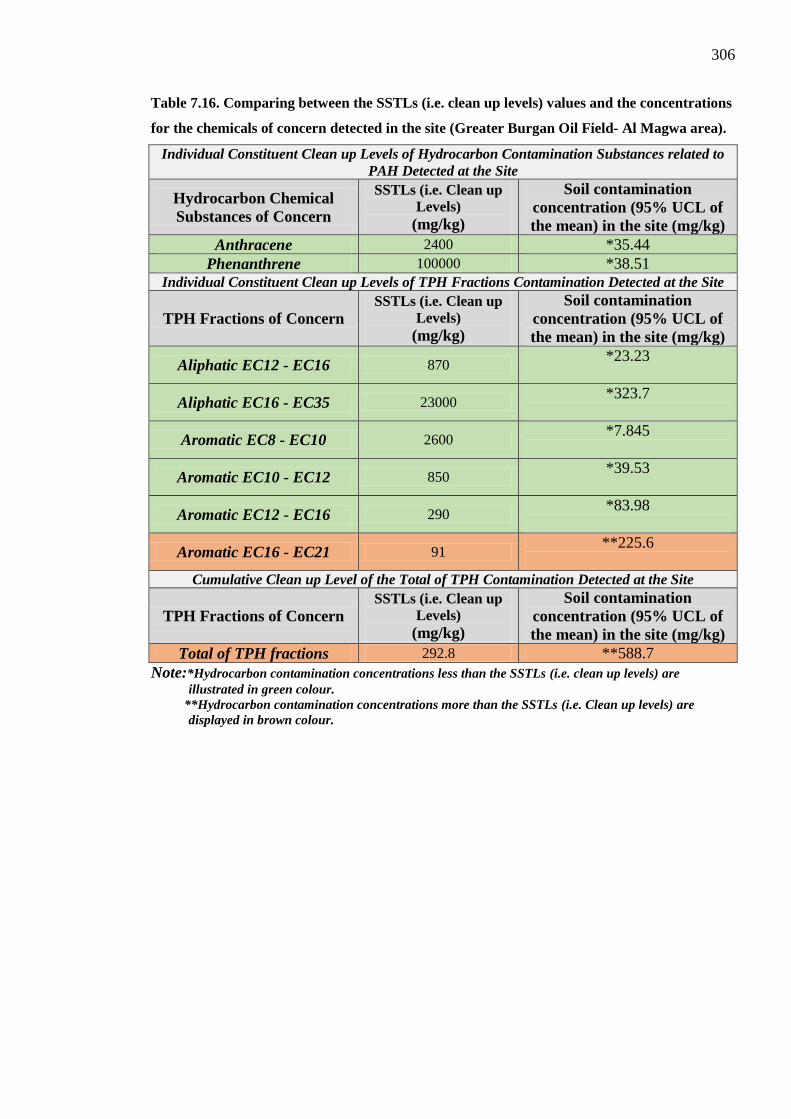
306
Table 7.16. Comparing between the SSTLs (i.e. clean up levels) values and the concentrations
for the chemicals of concern detected in the site (Greater Burgan Oil Field- Al Magwa area).
Individual Constituent Clean up Levels of Hydrocarbon Contamination Substances related to
PAH Detected at the Site
Hydrocarbon Chemical
Substances of Concern
SSTLs (i.e. Clean up
Levels)
(mg/kg)
Soil contamination
concentration (95% UCL of
the mean) in the site (mg/kg)
Anthracene 2400 *35.44
Phenanthrene 100000 *38.51
Individual Constituent Clean up Levels of TPH Fractions Contamination Detected at the Site
TPH Fractions of Concern
SSTLs (i.e. Clean up
Levels)
(mg/kg)
Soil contamination
concentration (95% UCL of
the mean) in the site (mg/kg)
Aliphatic EC12 - EC16 870 *23.23
Aliphatic EC16 - EC35 23000 *323.7
Aromatic EC8 - EC10 2600 *7.845
Aromatic EC10 - EC12 850 *39.53
Aromatic EC12 - EC16 290 *83.98
Aromatic EC16 - EC21 91 **225.6
Cumulative Clean up Level of the Total of TPH Contamination Detected at the Site
TPH Fractions of Concern
SSTLs (i.e. Clean up
Levels)
(mg/kg)
Soil contamination
concentration (95% UCL of
the mean) in the site (mg/kg)
Total of TPH fractions 292.8 **588.7
Note:*Hydrocarbon contamination concentrations less than the SSTLs (i.e. clean up levels) are
illustrated in green colour. **Hydrocarbon contamination concentrations more than the SSTLs (i.e. Clean up levels) are
displayed in brown colour.

307
7.6 Summary
This Chapter outlines the HHRA scenarios used for the contaminated site (dry oil lake at
Al-Magwa area), including: (1a) Hazard Identification; (1b) Hazard Assessment; (2a) Risk
Estimation; and (2b) Risk Evaluation. The HHRA scenarios followed in this study in order
to evaluate the carcinogenic and non-carcinogenic risks to human health and to calculate
clean-up levels needed for the identified locations-specifically for the safety of inhabitants
who may wish to reside in these area in the future. This Risk Evaluation was analysed by
means of RISC-5 modelling software. The following conclusions were drawn from these
analyses:
The human health (child and adult) carcinogenic risks caused by TPH fractions
(aliphatic and aromatic) and the chemicals associated with Anthracene and
Phenanathrene from the exposure into the assumed pathways at the site were
concluded as Not Detected (ND).
The influence of the non-carcinogenic risks on human health caused by the
Anthracene and Phenanathrene (PAH) and TPH fraction (aliphatic and aromatic)
contamination through the same assumed pathways show that the total HQ were 2.7
for children and 1.03 for adults, concluding that the HQ was > 1 which means a
potential risk.
The SSTLs, i.e. clean up levels‟ values were compared with the concentration of
hydrocarbon soil contaminants discovered at the site under study. The findings
clearly demonstrate that the detected contamination concentrations of the aromatic
(EC16 - EC21) hydrocarbon are greater than the calculated SSTLs. The total TPH
concentration of the site is also higher than the value of SSTLs, meaning that there
is a potential need for risk management measures.

308
8. DISCUSSION OF DEVELOPED SITE MODEL
8.1 Introduction
This chapter presents a discussion and interpretation of the correlation between the
geotechnical and geochemical characteristics of the hydrocarbon contaminated soil (see
Chapters 5 and 6). It also compares the relationship between the geotechnical and
geochemical properties of the hydrocarbon contaminated soil to the non-contaminated
(control) soil. A statistical analysis was conducted on the results of the laboratory data. The
analysis (in general) showed no appreciable changes to the characteristics of soil.
The Human Health Risk Assessment (HHRA) regarding the hydrocarbon contamination in
the soil (dry oil lake) in terms of non-carcinogenic risk values via the assumed pathways
are also discussed and evaluated. Additionally, the screening level values of the dry oil
lake site are compared with hydrocarbon concentrations and estimated for any site
designated for future development. This chapter also considers how Kuwaiti‟s human
health has been affected by hydrocarbon contaminations since the Iraqi invasion of
1991.To the best of the writer‟s knowledge no previous studies have been carried out to
research this relationship with soil contaminated with crude oil after a long drying-out
period (as in this study).
309
8.2 Geotechnical Properties
The effects of the hydrocarbon contamination on the geotechnical properties and the
interrelationship between these properties are discussed in this section.
8.2.1 Effect on Grain Size Distribution
As explained in section 5.3, hydrocarbon contamination of the silty sand soil in the dry oil
lake altered the grain size constituents of the original soil. It has led to an increase in the
percentage of large particles (more than 2.0 mm). This was clearly seen in samples taken
from the top soil where hydrocarbon contamination was found to be higher. However,
contamination was found to be decreasing at depths of approximately zero at 2.0 m from
the ground surface. Changes (see section 5.3) were attributed to the binding effect of the
dry oil lake residue on soil particles to cause an aggregation of several particles forming
one large particle during the sieving operation. This was clearer at the top soil level (0.0 m
depth).
The above phenomenon was justified from SEM photographs (Figures 5.14 to 5.16) for
samples taken from the top soil as further investigation of the grain size distribution took
place. An increase in the percentage of fine particles (less than 0.063 mm) was attributed to
the asphaltane particles left after drying of the oil lake residue. Statistical analysis proved
that contamination have significantly changed most of the grain size constituent
percentages. Such PSD variations seem to extend the soil away from being well graded, in
other words, the soil became closer to the uniformly or poorly graded.
The change to poorer gradation in the contaminated area was proved from statistical results
of Cc and Cu values (Section 5.3.2). The increase in the percentages of fine particles (less
than 0.063 mm) is in line with the study of Jia et al. (2011), who found higher clay
particles in severely polluted oil contamination (Section 3.3.1).

310
8.2.2 Effect on Permeability
As was clear from sections 5.3 and 5.4, contamination was high at shallow depths which
may have clogged some of the voids in soil at 0.25 m depth. However, at 0.0 m depth,
where the hydrocarbon contamination was higher it was expected to have been subjected to
a higher extent of drying than that of the 0.25 m depth leading to aggregations of some
particles (as shown in Figures 5.17 and 5.19) leading to coarser PSD; therefore, the
permeability at 0.0 m depth was higher than that at 0.25 m. This phenomenon was noticed
during the sampling process.
8.2.3 Reduction in Angle of Internal Friction (φ)
Referring to table 5.8 and figure 5.22, the angle of internal friction (φ) at the contaminated
site was shown to have been steadily decreased due to hydrocarbon contamination in all
samples. However, the decrease in internal friction angle (φ) due to hydrocarbon
contamination was generally lower as the depths increased. Statistical analysis proved that
the angle of internal friction (φ) was significantly increased with an increase in depth at the
contaminated area. However, in the non-contaminated area, there was no significant
change with depth (Figure 5.23). This phenomenon may be related to the reduced soil
contamination at greater depths.
As mentioned in section 5.6, the decrease of angle of internal friction (φ) in contaminated
soil may be related to hydrocarbon contamination changes to the PSD of soil to a poorer
grade. Although the reduction in the angle of friction does not appear to be high, (in this
study) due to contamination, it does cause an appreciable decrease in the angle of internal
friction of the soil.

311
8.3 Geochemical Properties
Clarification of the effects of oil contamination in the geochemical characterisation found
in the results of this study, i.e. changes in the acidity, chloride, sulphate, elementals, and
hydrocarbon contamination, will be provided in this section.
8.3.1 Change in the Acidity
For soils obtained from both contaminated and non-contaminated sites, it was found that
the contamination significantly increased the range between the maximum and minimum
pH values particularly at the top layer (which was expected to have higher contamination)
down to a depth of slightly more than 0.5 m. It was also found that the pH minimum values
of samples taken from the contaminated sites were significantly lower than for those from
the non-contaminated sites at all depths. This signifies that the hydrocarbon contamination
increases soil acidity. Although, this increase in acidity does not cause the soil to be
unsuitable for plant growth, it does, however, decrease its availability for agricultural
activities.
8.3.2 Effect on Chloride and Sulphate Content
As seen from the results in section 6.3, it is evident that the contamination of the chloride
has taken place through the whole 2.0 m investigated depth in the contaminated area. The
chloride content for the top layer of this area was found to be very high. Concentration
subsequently decreases with depth down 0.25 m below ground level, whereas, after the
0.25 m depth, it reaches an approximately constant value down to 2.0 m. At the non-
contaminated site, however, the chloride concentration was almost negligible. This
characteristic was proved statistically (see Figure 6.8) after deleting the outlier values. The
presence of high concentrations of chloride at the upper layer of the contaminated site
could be due to the higher hydrocarbon oil contamination.
312
Figures 6.5 and 6.6 in section 6.3 show that originally the soils had an appreciable sulphate
content (both SO3 and SO4). These contents were approximately constant at all depths in
the non-contaminated site. The figures also show that the sulphate contents of the very top
layer of the contaminated site were higher than that of the non-contaminated site. They
then drop down suddenly through the depths to become lower than that in the non-
contaminated site. Statistical analysis after deleting the outlier values proved this
phenomenon (see Figures 6.9 and 6.10). The lower content of SO3 and SO4 at depths lower
than the top layer may be attributed to the following interpretations:
A drop had taken place in the original sulphate (SO3 and SO4) of the
soil before its contamination which may be attributed to the proper
action of water in extinguishing the fires (Section 6.3).
The high concentration of sulphate still in the top layer comes from
high hydrocarbon contamination. However, during fire extinguishing
these sulphates may have been dissolved by the runoff from the fire
fighting materials and transported either vertically or horizontally
through the soil. Furthermore, statistical analysis showed that the depth
does not predict the concentration of sulphate (SO3 and SO4) at either
site.
8.3.3 Changes in the Carbon and Hydrocarbon Contamination with Depth
With the increase in depth, the mean values of carbon content (C %) in the contaminated
site was decreased considerably at depths down to 0.5 m; after that they drop to nearly
negligible values. However, in the non-contaminated area the carbon contents (C %) can
be considered as negligible at all depths (see Table 6.9 and Figure 6.16 shows C % values
after deleting outliers).

313
The above trend of relationships between the TPH concentrations with depths at the
contaminated site is noted. Statistical analysis proved that the TPH concentration at
the top layer was significantly higher than that at depths of 0.25 m and 0.5 m. TPH
was not encountered at lower depths (see Table 6.16).
8.4 Correlations in the Changes between Geotechnical and Geochemical Properties
Table (8.1) was prepared for the purpose of comparing changes
between the geotechnical and geochemical properties of the soil due to
contamination. The table displays multiple linear regression analysis
using the backward elimination technique which was performed on the
TPH concentration data for the contaminated site, to determine whether
four predictors (fine sand, curvature coefficient, angle of internal
friction, and SO4 at T.P.C. (50 m, 50 m) predict TPH concentration.
Results revealed that in the original program, model 1 of four predictors
had no significant impact on TPH, R2 = 0.992, F (4, 1) = 29.32, p=
0.138. The final model 4 included only that the angle of internal friction
was approaching significance, i.e. (B = -54.487, SEB = 20.090, Beta = -
0.805, p= 0.05).
From the above, it can be concluded that the angle of internal friction
was the best predictor in this model for TPH concentration. For every
one unit increase in angle of internal friction, the TPH concentration
decreased by 54.487 (mg / kg) units. On average, the R Square value of
0.648 indicates that the correlation between angle of internal friction
and TPH concentration is approximately 64.8 %.

314
Furthermore, there was virtually no (or very slight) changes in the
above characteristics below the 2.0 m depth (from the ground level).
This indicates that no crude oil residue contamination was taking place
under this layer and as such there is no concern regarding
contamination to the ground water, since the water table depth is more
than 10 m below the ground level.
Table 8.1. Multiple regression (Backward elimination technique) predicting TPH
concentration (mg/kg) from fine sand %, curvature coefficient (Cc), angle of internal friction
(φ) and SO4 (mg/kg) at T.P.C. (50 m, 50 m).
Model (Notes) Variable
Unstandardized
Coefficients
Standardized
Coefficients t-value p-value
B SE.B Beta
1 (All four predictors to
predict TPH)
(Constant) 3517.42 445.39 7.89 0.08
Fine Sand % 15.35 2.93 0.92 5.23 0.12
Curvature
coefficient (Cc) % -458.09 72.32 -1.34 -6.33 0.10
Angle of Internal
Friction (φ) -120.60 13.45 -1.78 -8.96 0.07
SO4
concentrations
(mg/kg)
0.10 0.04 0.36 2.21 0.27
2 (SO4 is excluded in
Model 2 as it was the least
significant predictor in
Model 1)
(Constant) 3918.85 699.24 5.60 0.03
Fine Sand % 11.59 4.11 0.70 2.81 0.10
Curvature
coefficient (Cc) % -393.86 113.86 -1.15 -3.45 0.07
Angle of Internal
Friction (φ) -124.74 22.89 -1.84 -5.44 0.03
3 (Fine sand % is
excluded in Model 3 as it
was the least significant
predictor in Model 2)
(Constant) 2646.99 972.64 2.72 0.07
Curvature
coefficient (Cc) % -155.77 139.03 -0.45 -1.12 0.34
Angle of Internal
Friction (φ) -76.31 27.55 -1.12 -2.77 0.07
4 (Only Angle of Internal
Friction is included in
final Model 4, as the best
predictor of TPH)
(Constant) 1811.80 644.44 2.81 0.04
Angle of Internal
Friction (φ) -54.48 20.09 -0.80 -2.71 *0.05
Note: -Dependent Variable: TPH Concentration.
-Coarse Sand, Medium Sand, and Exact Soil Passing number 230 predictor variables were excluded from this
backward elimination model. Linear regression found neither Coarse sand (B=-32.88, SEB=31.80, Beta=-.459,
p=.360), Medium Sand (B=10.294, SEB=8.757, Beta=0.507, p=0.305) and Exact Soil Passing No.230 (B=-17.037,
SEB=31.223, Beta=-0.263, p=0.614) predicted TPH concentration.
*indicates to the significant relationship between independent and dependent varaibles.
315
8.5 Human Health Risk Assessment (HHRA)
The investigation on geotechnical and geochemical properties detected hydrocarbon
concentrations on the site under investigation. Future expansion of Kuwait city is likely to
require development of these areas; as such a Human Health Risk Assessment (HHRA) of
the site has been carried out.
Thus, (in this section) the non-carcinogenic adverse impacts of the toxicity of hydrocarbon
contamination on human health through assumed pathways at the site were examined; the
clean-up level values for the contaminated site are also discussed in this section.
8.5.1 Non- Carcinogenic Risks through Investigated Pathways
Tables (7.14 & 7.15) and figures (7.16 & 7.17) show that the HQ is more than 1 for both
resident children and adults, which means that there is a potential health risk. Furthermore,
it can be clearly seen that a significant risk comes from the hydrocarbons through ingestion
of home-grown vegetables; this ingestion alone generates a HQ = 2.7 for child residents
(male and female) and 1.03 for adults (male and female). Therefore, if the home-grown
vegetables‟ pathway is removed in the area through the prohibition of such activities then
the human health risk will subsequently reduce as demonstrated by recalculated HQ of
0.34 for child (male and female) and 0.05 for adults (male and female) as such, there
would be no risk from the non-carcinogenic areas.

316
8.5.2 Estimation of Clean-up Levels for the Dry Oil Lake
Table 7.16 show that the aromatic EC16-EC21 and the total of TPH concentrations in the
site are higher than the site specific target levels (SSTLs). These values (above the SSTLs)
are justified as follows:
As principle deriving risk to the health of child and adult residents (both
male and female) was constituted through the aromatic (EC16 - EC21)
hydrocarbons.
The TPH fractions‟ concentrations of HQ < 1 are considered to be
acceptable. However, it is evident that the total of these TPH fraction
concentrations for the whole site will constitute a potential risk to the
health of both children and adult residents (male and female) in the
future (HQ >1) (Tables 7.14 and 7.15).
The results indicate that there is need for risk management measures for not only home-
grown vegetables but also other agricultural activities in the dry oil lake site (al-Magwa
area) for the protection of future residents.

317
9. FINAL CONCLUSIONS
9.1 General Overview
Following the Gulf War in 1990 and the extinguishing of the oil fires on the Greater
Burgan Oil Field (Al-Magwa area), the resulting dry oil lakes were left untouched for 23
years. During this time changes to the geotechnical and geochemical properties of the near
surface soil found in these lakes occurred. In particular, the level of detectable
hydrocarbons and their subsequent effects on the soil at ground surface were found to have
decreased to very low levels at typical normal building foundation depths. As such, it can
be assumed that there has been no subsequent contamination of the ground water from this
dry oil lake, as the ground water level is typically found at around 10 m below ground
level.
This study has also clearly shown that hydrocarbons exist in the upper soil layer (0.0 m -
0.5 m depth), despite having been exposed to a hot arid environment since the initial
polluting events of the Gulf War in 1990.
9.2 Geotechnical Properties
This study has shown that the hydrocarbon contamination in a dry oil lake influences the
particle size distribution (PSD) and decreases the shear strength of the soil and has
complicated effects on permeability in the upper soil layer. In particular:
Effect on grain size distribution: Hydrocarbon contamination aggregates
the grains at the upper soil layer, increasing the percentages of gravel size
particles (more than 2.0 mm). The overall effect was change in the soil
gradation to a poorer one.

318
Mechanism of change in permeability: The permeability was
significantly decreased to depth 0.25 m although it was not affected to any
considerable extent (at depth 0.0 m due to contamination) (this
phenomenon is discussed in section 8.2.2), because of the complication of
clogging with some of the voids by the dried oil and changes in the PSD to
poorer grade.
Reduction in Angle of Internal Friction: This reduction has been shown
to be related to the aggregation of the soil particles in the upper soil layer,
leading to poorer PSD. The overall effect being shown to decrease linearly
with depth (Figures 5.20 & 5.22).
9.3 Geochemical Properties
This study has shown that the hydrocarbon contamination in a dry oil lake causes alteration
in the acidity, the soluble chloride and the soluble sulphate contents at varying depths in
the near ground surface soil layers. In particular:
Change in the Acidity: Hydrocarbon contamination causes an increase in
the acidity of the soil. The increase in acidity, however, was not so great as
to lower the soil cultivation activity to unsuitable, whereas the minimum
pH values of the soil samples for the contaminated site was classified in
the range of neutral values (6.6 - 7.3) (Horneck et al., 2011).
Effect on the chloride and sulphate content: It appears that hydrocarbon
contamination results in a very high chloride content particularly of the
upper soil layer.
High soluble sulphate content has also been detected, at the top layer (0.0
m), however, it decreased to a lower value than that at the non-
contaminated site which may have been the result of runoff from the
319
firefighting process. This runoff may have further dissolved the sulphate
contents in the original soil (prior to hydrocarbon contamination). A
decrease in both the soluble chloride and sulphate content at depth have
been shown to occur at the contaminated site.
Hydrocarbon content: The hydrocarbon content of the upper soil layer
has been shown to decrease with depth (0.0 m - 0.5 m), until negligible at
a depth of 1.0 m.
9.4 Human Health Risk Assessment (HHRA)
The Human Health Risk Assessment has given the following results:
The largest influencing pathway is the ingestion of home-grown
vegetables. Consequently, if this pathway is removed from the area
through the prohibition of such home-grown vegetable production and
agricultural activities then the human health risk will be reduced (HQ < 1),
therefore, there would be no health risk from the non-carcinogenic areas
for residents, i.e. child and adults (see Tables 7.14 & 7.15 in section 7.5.4).
The key hydrocarbon contaminant of concern was identified as aromatic
EC16 - EC21 hydrocarbons.
The total of TPH concentration (mg/kg) at the site (Al-Magwa area)
exceeds the calculated SSTL value (mg/kg).
Any future development of dry oil lake sites should include relevant
risk management measures for home-grown vegetables and other
agricultural activities to remove the potential ingestion pathway.

320
10. FINAL RECOMMENDATIONS FOR FURTHER
WORK
As mentioned by North (2000), cancer and respiratory related diseases have multiplied
substantially in Kuwait since the Iraqi invasion of the 1990s. It has been suggested that the
increase in these illnesses may be attributed to the following factors:
The presence of hydrocarbon contamination for the last 25 years (currently
being studied) in open spaces which have had no remediation; this has
seriously affected the whole area.
The rapid rise in the population of Kuwait since 1991, which has led to an
increase in residential development and subsequently slow encroachment
onto the „dry oil lakes‟.
The hot and arid climate of Kuwait caused high evaporation rates from the
abandoned hydrocarbon oil lakes into the atmosphere thus potentially
directly affecting Kuwaiti residents. Dr. Al-Ghanim (HICT, 2011)
mentioned that a large proportion of asthmatic sufferers come from the
southern area of Kuwait which is close to the Greater Burgan Oil Field
(current study).

321
Therefore, in respect of future plans of the Kuwaiti Government to expand the residential
area near the Greater Burgan Oil Field, further studies are recommended as shown below:
Implementation of similar studies are recommended for nearby oil lakes to
consider the full extent of hydrocarbon contamination at depth.
Investigation into probable hydrocarbon contamination of the ground
water would be beneficial.
Development of a wider ground model of the long term migratory
behavior of hydrocarbons from the dry oil lakes.
Application of RISC-5 software or other suitable software to develop
lateral vapor and particulates‟ models suitable to the ground conditions
encountered at the study site.
Further investigation into changes to the angle of internal friction
related to contact with the hydrocarbon residue.
Investigation into the effects of the measured chloride and sulphate
contents on likely concrete foundations.
322
REFERENCES
Abramson, M. J., Forbes, A. B., Glass, D. C., Ikin, J. F., Ittak, P., Kelsall, H. L.,
McKenzie, D. P., & Sim, M. R. (2004). Respiratory health status of Australian
veterans of the 1991 gulf war and the effects of exposure to oil fire smoke and dust
storms. Thorax, 59(10), 897-903.
Agency for Toxic Substances and Disease Registry, (ATSDR). (1999). Toxicological
profile for Total Petroleum Hydrocarbons (TPH). U.S. department of health and
human services public health service. Retrieved from Agency for Toxic Substances
and Disease Registry website: http://www.atsdr.cdc.gov/ToxProfiles/tp123.pdf
Ahamad, Al R. & Barker, C. (2011). Role of evaporation in degrading the “oil lakes”.
American Journal of Environmental Sciences, 7(3), 219 - 223.
Al-Ajmi, D. (1994). Simulation of short term atmospheric dispersion of SO2 resulting
from the Kuwait oil fires. In F. El-Baz, & R. M. Makharita (Eds.), The Gulf War
and the environment (pp. 69-83). Amsterdam: Gordon and Breach Science
Publishers S.A.
Al-Ajmi, D., Misak, R., Khalaf, F. I., Al-Sudairawi, M., & Al-Dousari, A. M. (1994).
Damage assessment of the desert and coastal environment of Kuwait by remote
sensing (VT001C) (Report No. 4405). Kuwait: Kuwait Institute for Scientific
Research.
Al-Ajmi, D., & Marmoush, Y. (1996). Ground level concentration of sulfur dioxide at
Kuwait's major population centers during the oil-field fires. Environment
International, 22(3), 279-287.
Al-Ajmi, D., Misak R., Al-Ghonaim M., & Mahfooz S. (1997). Oil trenches .The
destructions of the environment of the state of Kuwait. Kuwait: Center for Research
and Studies of Kuwait.
323
Al-Ali, E. H. (2008).Groundwater history and trends in Kuwait. WIT Transactions on
Ecology and the Environment, 112, 153-164.
Al-Awadhi, N., Abdal, M. S., Briskey, E. J., & Williamson, K. (1992). Assessment of
technologies for the remediation of oil-contaminated soil resulting from exploded
oil wells and burning oil fires in Kuwait. Proceeding of Air and Waste Management
Association Meeting, 26(1), 21-26.
A1-Awadhi, N., Williamson, K. J., & Isok, J. D. (1993). Remediation of Kuwait's oil-
contaminated soils. In P.T. Kostecki & E. J. Calabrese (Eds.), Hydrocarbon
Contaminated soil and groundwater (pp. 9-21) London: Lewis Publishers.
Al-Awadhi, N., Al-Daher, R., El-Nawawy, A., & Baiba, M. T. (1996). Bioremediation of
oil-contaminated soil in Kuwait, land farming to remediate oil-contaminated soil.
Soil and Sediment Contamination, 5(3), 243-260.
Al-Awadi, E., Al-Ruwaih, F., Al-Rawdan, Z., & Ozkaya, I. (1997). The stratigraphy of the
middle eocene–pleistocene sediments in Kuwait. Journal of Arid Environments,
37(1), 1–22.
Al-Awadhi, J. M., Omar, S. A., & Misak, R. F. (2005). Land Degradation Indicators in
Kuwait. Land Degradation & Development, 16(2), 163–176.
Al-Besharah, J. (1991). The Kuwait oil fires and oil lakes- facts and numbers. In A. K. S.
Al-Shatti, & J. M. Harrington (Eds.), Proceedings of the environmental and health
impact of the Kuwaiti oil fires (pp. 12-15.). Birmingham, UK: University of
Birmingham.
Al-Besharah, J., & Salman, M. (1991). Assessment of the oil lakes in Kuwait’s oil fields
(Report No. 4005). Kuwait: Kuwait Institute for Scientific Research (KISR).
Al-Besharah, J., Salman, M. & Al-Matrook, F. (1992). Characterization and quantification
of reclaimable oil from oil lakes formed in Kuwait oil fields (Report No. 4081).
Kuwait: Kuwait Institute for Scientific Research.
324
Al-Dousari, A. (2001). Analysis of change in the tarcrete layer on the desert surface of
Kuwait using satellite imagery and cell-based modelling (Unpublished doctoral
thesis). Boston University, United States.
Al-Duwaisan. D. B., & Al-Naseem A. A. (2011). Characterization of oil contaminated soil
Kuwait oil lakes. Proceedings of 2nd International Conference on Environmental
Science and Technology (ICEST):Vol. 6. (pp. 439-442). Singapore: IACSIT Press.
Alhassan H. M., & Fagge S. A. (2013). Effects of crude oil low point pour fuel oil and
vacuum gas oil contamination on the geotechnical properties sand, clay and laterite
soils. International Journal of Engineering Research and Applications (IJERA),
3(1), 1947-1954.
Al-Jassar, H. K., & Rao, K. S. (2010). Monitoring of soil moisture over the Kuwait desert
using remote sensing techniques. International Journal of Remote Sensing, 31(16),
4373-4385.
Al-Khaled, O., Al-Zuabi, Y., Edwards, K., Hafez, M., & Sulistiono, D. (2012).
Geostatistical inversion in carbonate and clastic reservoirs: Oilfield case studies
from Kuwait. GeoConvention, 1-8. Retrieved from
http://webcache.googleusercontent.com/search?q=cache:aVY__H04AjYJ:www.ge
oconvention.com/archives/2012/093_GC2012_Geostatistical_Inversion_in_Carbon
ate_and_Clastic_Reservoirs.pdf+&cd=1&hl=en&ct=clnk&gl=uk
Al-Kulaib, A. A. (1984). The climate of Kuwait (Directorate General of Civil Aviation:
Meteorological Department). Kuwait: Directorate General of Civil Aviation.
Allison, T. R. (1969). Particular problems encountered in building and civil engineering
design and construction in the State of Kuwait. (Report of the Government
Research Station). Kuwait: Ministry of Public Works.
Almarshad, A. A. M. A. (2014). BIM-based knowledge management system for building
maintenance (Doctoral thesis, Heriot Watt University, Edinburgh, UK). Retrieved
from http://www.ros.hw.ac.uk/handle/10399/2770

325
Al-Rashed, M. F., & Sherif, M. M. (2001). Hydrogeological aspects of groundwater
drainage of the urban areas in Kuwait city. Hydrological Processes, 15, 777–795.
Al-Rashed, M., Mukhopadhyay, A., Al-Senafy, M., & Ghoneim, H. (2010). Contamination
of groundwater from oil field water disposal pits in Kuwait. The Arabian Journal
for Science and Engineering, 35(1B), 105-123.
Al-Saad, A. (1993). Oil lakes. Lecture presented at Kuwait engineering society, Kuwait, p.
32.
Al-Sanad, H. A., Eid, W. K., & Ismael, N. F. (1995). Geotechnical properties of oil-
contaminated Kuwaiti sand. Journal of Geotechnical Engineering-ASCE, 121(5),
407- 412.
Al-Sanad, H. A., & Ismael, N. F. (1997). Aging effects on oil-contaminated Kuwaiti sand.
Journal of Geotechnical and Geo-environmental Engineering, 123(3), 290-293.
Al-Sarawi, M., & Massoud, M. S., Al-Abdali, F. (1998a). Preliminary assessment of oil
contamination levels in soils contaminated with oil lakes in the Greater Burgan oil
Fields, Kuwait. Water, Air, and Soil Pollution, 106(3), 493 – 504.
Al-Sarawi, M., Massoud, M. S., & Wahba, S. A. (1998b). Physical properties as indicators
of oil penetration in soils contaminated with oil lakes in the Greater Burgan Oil
Fields, Kuwait. Journal of Water, Air, and Soil Pollution, 102, 1–15.
Alsharhan, A. S., Rizk, Z. A., Nairn, A. E. M., Bakhit, D. W. and Al-hajari, S. A. (2001).
Hydrogeology of an Arid Region: The Arabian Gulf and Adjoining Areas (1st ed.).
Amsterdam, Netherlands: Elsevier.
Al-Sulaimi, J., & Mukhopadhyay, A. (2000). An overview of the surface and near-surface
geology, geomorphology and natural resources of Kuwait. Journal of Earth-
Science Reviews, 50 (3-4), 227-267.
Al-Sulaimi, J. S., & Al-Ruwaih, F. M. (2004). Geological, structural and geochemical
aspects of the main aquifer systems in Kuwait. Kuwait Journal of Science and
Engineering, 31(1), 149-174.

326
Al-Yaqout, A., & Townsend, F. (2004). Applicability of calcite (Gatch) as linear/cover in
arid climate landfills: Laboratory and field permeability. Practice Periodical of
Hazardous, Toxic and Radioactive Waste Management, 8(4), 238-246.
Amat-Bronnert, A., Castegnaro, M., & Pfohl-Leszkowicz, A. (2007). Genotoxic activity
and induction of biotransformation enzymes in two human cell lines after treatment
by Erika fuel extract. Environmental Toxicology Pharmacology, 23(1), 89–95.
American Society of the International Association for Testing and Materials (ASTM).
(2000). Standard Practices for Preserving and Transporting Soil Samples (Report
No. D 4220-95). United States: ASTM.
American Society of the International Association for Testing and Materials (ASTM).
(2008). Standard test method for density of soil in place by the drive-cylinder
method (Report No. D 2937-04). United States: ASTM.
Amro, M. (2004). Treatment Techniques of Oil-Contaminated Soil and Water Aquifers.
Proceedings of the 1st International Conference on Water Resources and Arid
Environment (pp. 1-11.). Riyadh, Saudi Arabia: Petroleum Engineering
Department, King Saud University.
Angehrn, D. (1998). Risk assessment for residual mineral oil contaminants in
bioremediated soil (Doctoral thesis, Swiss federal Institute of Technology, Zurich).
Retrieved from http://e-collection.library.ethz.ch/eserv/eth:22907/eth-22907-02.pdf
Anthraquinone, 1,2,3,4-tetrahydro-. (n.d.). ChemSpider: Search and share chemistry
database. Retrieved from http://www.chemspider.com/Chemical-
Structure.190099.html?rid=6d1f58e0-7143-4263-872e-55b0f643da85
Arab sustainability Association (ASA). (2012). Kuwait Environment Public Authority
plays major role in safeguarding environment. Retrieved from Arab sustainability
Association website: http://www.ifpinfo.com/asa/asa-news.php?news_id=343
Armah, F. A., Kuitunen, M., Luginaah, I., & Mkandawire, P. (2012). Non occupational
health risk assessment from exposure to chemical contaminants in the Gold mining
327
environment of Tarkwa, Ghana. Trends in Applied Sciences Research, 7(3), 181-
195.
Asharaf, I. (2011, November). Risk based assessment of contaminated land &
groundwater. Paper presented at the meeting of the 20th Joint GCC- Japan
Environment Symposium-4th Joint UAE- Japan Environment Symposium.
Baah, B. (2011). Phytoremediation of hydrocarbon contaminated soil-a case study at
Newmont Ghana gold limited-ahafo kenyasi (Master dissertation, Kwame Nkrumah
university of science and technology, Ghana). Retrieved from
http://ir.knust.edu.gh/bitstream/123456789/4074/1/PHYTOREMEDIATION%20FI
NAL%20FINAL%20FINAL%20%2005-01-12.pdf
Balba, M. T., Al-Daher, R., & Al-Awadhi, N. (1998). Bioremediation of oil-contaminated
desert soil: The Kuwait experience. Environment International, 24(1/2), 163-173.
Barker, C., & Bufarsan, A. (2001). Evaporative losses from the surfaces oil lakes of
southern Kuwait. Environmental Geosciences, 8(2), 123-129.
Barnett, F., Singh, A. & Singh, A. K. (2013). Statistical Software for Environmental
Applications for Data Sets with and without Nondetect Observations (ProUCL
Version 5.0.00 Technical Guide), Washington, DC: U.S. Environmental Protection
Agency Office of Research and Development.
Barua, D., Buragohain, J., & Sarma, S. K. (2011). Certain physico-chemical changes in the
soil brought about by contamination of crude oil in two oil fields of Assam, NE
India. European Journal of Experimental Biology, 1(3), 154-161.
Bashara, J. (1991). Oil Lakes Committee, Phase One, Kuwait Foundation of Advancement
of Science. Kuwait.
Benyahia, F., Abdulkarim, Mzekri, A., Chaalal, O., & Hasanain, H. (2005).
Bioremediation of crude oil contaminated soils a black Art or an engineering
challenge. Process Safety and Environmental Protection. 83(4), 364 – 370.
328
Blaisdell, R. A., & Smallwood, M. E. (1993). Evaluation of the Total Petroleum
Hydrocarbon Standard for Cleanup of Petroleum Contaminated Sites (Master
dissertation). Air University, United States.
Bowers, R. L., & Smith, J. W. N. (2014). Constituents of potential concern for human
health risk assessment of petroleum fuel releases. Quarterly Journal of Engineering
Geology and Hydrogeology, 47(4), 363 - 372.
Bregnard, T. P., Höhener, P., & Zeyer, J. (1998). Bioavailability and biodegradation of
weathered diesel fuel in aquifer material under denitrifying conditions. Journal of
Environmental Toxicology and Chemistry, 17(7), 1222-1229.
Bretzler, A. (n.d.). Hydrocarbon contamination of groundwater in Kuwait due to the Gulf
war. 4th Year Environmental Science (Geoecology), 1-9. Retrieved from
http://www.geo.tu-
freiberg.de/~hasche/S_Grundwasserschutz/Paper_GWS_Anja_Bretzler.pdf
Brewer, R., Nagashima, J., Kelley, M., Heskett, M., & Rigby, M. (2013). Risk-based
evaluation of Total Petroleum Hydrocarbons in vapor intrusion studies.
International Journal of Environmental Research and Public Health, 10(6), 2441-
2467.
British Columbia (BC) (n.d.). Polycyclic Aromatic Hydrocarbons (PAHs): 2.0 PAHs and
their characteristics. Retrieved from
http://www.env.gov.bc.ca/wat/wq/BCguidelines/pahs/pahs-01.htm
British standard Institution (BSI). (1990a). Methods of test for Soils for civil engineering
purposes-Part 2: Classification tests (Report No. BSI-1377-2:1990). Incorporating
Amendment No. 1. London, UK: BSI.
British standard Institution (BSI). (1990b). Methods of test for Soils for civil engineering
purposes-Part 5 (Report No. BSI-1377-5:1990): Compressibility, permeability and
durability tests. Incorporating Amendment No. 1. London, UK: BSI.

329
British Standard Institution (BSI). (1990c). Methods of test for Soils for civil engineering
purposes-Part 3: Chemical and electro-chemical tests (Report No. BSI-1377-
3:1990). Incorporating Amendment No. 1. London, UK: BSI.
Bufarsan, A., Barker, C., Wavrek, D. A., & Al-Sarawi, M. (2002). Compositional changes
induced by evaporation of Burgan crude oil spilled into the desert of southern
Kuwait. Environmental Geosciences, 9(1), 8-16.
Bul, I. D. (2008). Gas Chromatography Mass Spectrometry (GC-MS). Retrieved from
http://www.bris.ac.uk/nerclsmsf/techniques/gcms.html
Butylated Hydroxy Toluene (BHT). (n.d.). ChemSpider: Search and share chemistry
database. Retrieved from http://www.chemspider.com/Chemical-
Structure.13835296.html?rid=39fb7659-f9ed-4389-a8ac-ed3c1c2bc137
Campbell D., Cox, D., Crum, J., Foster, K., Chrístie, P., & Brewster, D. (1993). Initial
effects of the grounding of the tanker Braer on health in Shetland. British Medical
Journal (BMJ), 307(6914), 1251–1255.
Caravaca, F., & Roldan, A. (2003). Assessing changes in physical and biological properties
in a soil contaminated by oil sludges under semiarid mediterranean conditions.
Journal of Geoderma, 117(1-2), 53-61.
Carman, G. J. (1996). Structural elements of onshore Kuwait. GeoArabia, 1(2), 239-266.
Casagrande, A. (1984). Classification and identification of soils. Journal of Transactions
of the American Society of Civil Engineers (ASCE), 113(1), 901-930.
Cedergren, H. R. (1997). Seepage, drainage and flow nets (3rd ed.). New York: John
Wiley & Sons.
Certini, G., Scalenghe, R., & Woods, W. (2013). The impact of warfare on the soil
environment. Earth-Science Reviews, 127, 1-15.
Chavicol. (n.d.). ChemSpider: Search and share chemistry database. Retrieved from
http://www.chemspider.com/Chemical-Structure.21105856.html?rid=4357a944-
f89a-4173-9d68-e2d5ea1ab94b
330
Chen, K., Wu, L., Kao, C. & Yang, C. (2004). Application of health risk assessment to
derive cleanup levels at a fuel-oil spill site. Practice Periodical of Hazardous,
Toxic, and Radioactive Waste Management, 8(2), 99–104.
Cho, B., Chino, H., Tsuji, H., Kunito, T., Nagaoka, K., Otsuka, S., Yamashita, K.,
Matsumoto, S., & Oyaizu, H. (1997). Laboratory-scale bioremediation of oil-
contaminated soil of Kuwait with soil amendment materials. Journal of
Chemosphere, 35(7), 1599-1611.
Churngold (n.d.). Hydrocarbon contamination. Retrieved from
http://www.churngold.com/remediation/problems/hydrocarbon-contamination.html
Contaminated Land: Applications in Real Environments (CL: AIRE). (2014). SP1010 -
Development of category 4 screening levels for assessment of land affected by
contamination (Final Project Report (Revision 2)). London, UK: CL: AIRE.
Department for environment, Food and Rural Affairs (DEFRA). (2005). Soil guideline
values for naphthalene contamination (R&D publication SGV 19). Bristol:
Environmental Agency.
Dimethylanthracene. (n.d.). ChemSpider: Search and share chemistry database. Retrieved
from http://www.chemspider.com/Chemical-Structure.31706.html?rid=deb3fdfc-
acd5-4252-aff8-abc8f8a88b7c
Dimethylbenzothiophene. (n.d.). ChemSpider: Search and share chemistry database.
Retrieved from http://www.chemspider.com/Chemical-
Structure.556117.html?rid=efb38e1d-f95e-
Dimethyldibenzothiophene. (n.d.). ChemSpider: Search and share chemistry database.
Retrieved from http://www.chemspider.com/Chemical-
Structure.158333.html?rid=57a8e02f-4a9a-4137-8490-33bff13fd65f
Dimethylsilanediol. (n.d.). ChemSpider: Search and share chemistry database. Retrieved
from http://www.chemspider.com/Chemical-Structure.13396.html
331
Din, S., Al Dousari, A., & Literathy, P. (2008). Evidence of hydrocarbon contamination
from the Burgan oil field, Kuwait-Interpretations from thermal remote sensing data.
Journal of Environmental Management, 86(4), 605–615.
Dionex. (2011). Accelerated Solvent Extraction (ASE) of hydrocarbon contaminants
(BTEX, Diesel and TPH) in soils (Application Note 324).Thermo Fisher Scientific,
Salt Lake City, UT, USA.
Di-p-Tolylacetylene. (n.d.). ChemSpider: Search and share chemistry database. Retrieved
from http://www.chemspider.com/Chemical-Structure.453892.html
Docosane. (n.d.). ChemSpider: Search and share chemistry database. Retrieved from
http://www.chemspider.com/Chemical-Structure.11899.html
Dodecane. (n.d.). ChemSpider: Search and share chemistry database. Retrieved from
http://www.chemspider.com/Chemical-Structure.7890.html?rid=323e037b-2db9-
4500-8bec-e3185bdbd753
Dumitran, C., & Onutu, I. (2010). Environmental risk analysis for crude oil soil pollution.
Carpathian Journal of Earth and Environmental Sciences, 5(1), 83 - 92.
El-Baz, F., Abuelgasim, A., Koch, M., Pax-Lenney, M., Lambin, E., Al Doasari, A., Marr,
P., Ryherd, S., & Morency, R. (1994). Detection by satellite images of
environmental change due to the Gulf war. In F. El-Baz, R. M. Makharita (Eds.),
The gulf war and the environment (pp. 1–24.). Lausanne: Gordon and Breach
Science.
Elisha, A. T. (2012). Effect of crude oil Contamination on the geotechnical properties of
soft clay soils of Niger delta region of Nigeria. Electronic Journal of Geotechnical
Engineering (EJGE), 17, 1929 - 1938.
Environment Agency. (2003). Principles for evaluating the Human Health Risks from
petroleum hydrocarbons in soils: A Consultation Paper (Report P5-080/TR1). UK,
Bristol: Environment Agency.
332
Environment Agency. (2005). The UK Approach for evaluating Human Health Risks from
petroleum hydrocarbons in Soils (Report P5-080/TR3). UK, Bristol: Environment
Agency.
Ezilon. (2015). Kuwait map-political map of Kuwait. Retrieved from
http://www.ezilon.com/maps/asia/kuwait-maps.html
Field, A. P. (2009). Discovering Statistics Using SPSS (3rd ed.). London: Sage.
Foreign and Commonwealth Office of UK. (2014). GCC Economics summary (Foreign
and Commonwealth Office). Retrieved from gov.uk website:
https://www.gov.uk/government/uploads/system/uploads/attachment_data/file/3606
92/REST_GCC_Economics_Summary_for_July_and_August_2014_-_PRV.pdf
Four, 6-dimethyldibenzothiophene. (n.d.). ChemSpider: Search and share chemistry
database. Retrieved from http://www.chemspider.com/Chemical-
Structure.1064783.html
(Fourteen β)-Pregnane. (n.d.). ChemSpider: Search and share chemistry database.
Retrieved from http://www.chemspider.com/Chemical-Structure.23253685.html
Gay, J., Shepherd, O., Thyden, M., & Whitman, M. (2010). The health effects of oil
contamination: A compilation of research (E-project-121510-203112).
Washington, DC: Worcester Polytechnic Institute.
Geochemical Instrumentation and Analysis (GIA). (n.d.). Scanning Electron Microscopy
(SEM). Retrieved from
http://serc.carleton.edu/research_education/geochemsheets/techniques/SEM.html
Goi, A., Trapido, M., & Kulik, N. (2009). Contaminated Soil Remediation with Hydrogen
Peroxide Oxidation. World Academy of Science, Engineering and Technology, 52,
185 - 189.
Google Map (GM). (n.d.). Google map. Retrieved from
https://www.google.co.uk/maps/place/Kuwait/@29.0456051,48.0382788,10z/data=
333
!4m5!3m4!1s0x3fc5363fbeea51a1:0x74726bcd92d8edd2!8m2!3d29.31166!4d47.4
81766
Green Cross International (GCI). (1998, June). Addressing environmental consequences of
war: background paper. Paper presented at the 1st International Conference on
Addressing Environmental Consequences of War.
GSI Environmental (2014). RBCA tool kit for chemical releases. Retrieved from
http://www.gsi-net.com/en/software/rbca-software-tool-kit-for-chemical-releases-
version-2-6.html
Gupta, M. K., & Srivastava, R. K. (2010). Evaluation of engineering properties of oil-
contaminated soils. Journal of the Institution of Engineer India, 90, 37-42.
Habib-ur-Rahman, Abduljauwad, S. N., & Akram, T. (2007). Geotechnical behavior of oil
-contaminated fine grained soils. Electronic Journal of Geotechnical Engineering
(EJGE), 12. Retrieved from http://www.ejge.com/2007/Ppr0720/Ppr0720.htm
Hadi, K. (n.d.). The impacts of oil lakes on the fresh groundwater lenses in Kuwait. Water
Resources Division, 163-172. Retrieved from
http://aguas.igme.es/igme/publica/pdflib15/015.pdf
Healthcare Information and Communication Technology (HICT). (2011). Middle East
Healthcare News: Asthma rate is increasing furiously in Kuwait. Retrieved from
http://blog.ictforhealth.com/2010/11/asthma-rate-is-increasing-furiously-in-kuwait/
Heneicosane. (n.d.). ChemSpider: Search and share chemistry database. Retrieved on
from http://www.chemspider.com/Chemical-Structure.11897.html
Heptadecane. (n.d.). ChemSpider: Search and share chemistry database. Retrieved from
http://www.chemspider.com/Chemical-Structure.11892.html?rid=feb90bd2-3551-
4303-b8fd-219a15e0c9fe
Hesnawi, R. M., & Adbeib, M. M. (2013). Effect of nutrient source on indigenous
biodegradation of diesel fuel contaminated soil. Journal of APCBEE Procedia, 5,
557–561.
334
Hexadecane. (n.d.). ChemSpider: Search and share chemistry database. Retrieved from
http://www.chemspider.com/Chemical-Structure.10540.html?rid=c09bc837-11a7-
4012-a2fc-165091232243
Hoaglin, D.C., Iglewicz, B., & Tukey, J.W. (1986). Performance of some resistant rules for
outlier labeling, Journal of American Statistical Association, 81(396), 991-999.
Horneck, D. A., Sullivan, D. M., Owen, J. S., & Hart. J. M. (2011). Soil test interpretation
guide. Retrieved from https://catalog.extension.oregonstate.edu/ec1478
Hosford, M. (2009). Using science to create a better place: human health toxicological
assessment of contaminants in soil (Science Report – Final SC050021/SR2).
Bristol: Environment Agency.
Hua, Y., Luo, Z., Cheng, S., & Xiang, R. (2012). Health risks of organic contaminated soil
in an out-of-service oil refinery site. Journal of Earth Science, 23(1), 121–128.
Husain, T. (1998). Terrestrial and atmospheric environment during and after the Gulf war.
Environment International, 24(1), 189-198.
Hussain, T. (1995). Kuwait Oil Fires, Regional Environmental Perspective (1st ed.).
Oxford, UK: Pergamon Press Ltd.
Icosane. (n.d.). ChemSpider: Search and share chemistry database. Retrieved from
http://www.chemspider.com/Chemical-Structure.7929.html
Ijimdiya, T. S. (2013). The effects of oil contamination on the consolidation properties of
lateritic soil. Development and Applications of Oceanic Engineering (DAOE), 2(2),
53 -59.
INCO, (2007). Soil investigation for new 16 “HP GAS LINE FROM” “F” manifold to GC-
22 at KOC, Al-Magwa Area (Near GC-22), (Unpublished Report contract
No.27333, owiner: Kuwait oil company (KOC), on behalf of: Specialist oilfield
services company, prepared by: INCO-lab for testing materials soil surveying).
North Subhan, Kuwait.
335
Indane. (n.d.). ChemSpider: Search and share chemistry database. Retrieved from
http://www.chemspider.com/Chemical-Structure.9903.html
International Agency for Research on Cancer (IARC). (1989). Iarc monographs On the
evaluation of carcinogenic risk to humans: occupational exposure in petroleum
refining; crude on and major petroleum fuels (Volume 45). Retrieved from World
Health Organization website:
file:///C:/Users/user/Desktop/final%20editing%20in%20major%20correction-
statistics/Kuwait%20crude%20oil%20report.pdf
Irvine, G. M., Blais, J. M., Doyle, J. R., Kimpe, L. E., & White, P. A. (2014). Cancer risk
to First Nations’ people from exposure to polycyclic aromatic hydrocarbons near
in-situ bitumen extraction in Cold Lake, Alberta. Environmental Health, 13(7).
Retrieved from https://ehjournal.biomedcentral.com/articles/10.1186/1476-069X-
13-7
Iso hexadecane. (n.d.). ChemSpider: Search and share chemistry database. Retrieved from
http://www.chemspider.com/Chemical-Structure.19228.html
Iturbe, R., Flores, R. M., Flores, C. R., & Torres, L. G. (2004). TPH-contaminated
Mexican refinery soil: health risk assessment and the first year of changes.
Environmental Monitoring Assessment, 91(1-3), 237-255.
Jean-Philippe, S. R., Labbé, N., Franklin, J. A. & Johnson, A. (2012). Detection of
mercury and other metals in mercury contaminated soils using mid-infrared
spectroscopy. The International Academy of Ecology and Environmental Sciences,
2(3), 139-149.
Jeffries, J., & Martin, I. (2009). Updated technical background to the CLEA model
(Science Report: SC050021/SR3). Bristol: Environment Agency.
Jia, Y., Wu, Q., Shang, H., Yang, Z., & Shan, H. (2011). The influence of oil
contamination on the geotechnical properties of coastal sediments in the Yellow
336
River Delta, China. Bulletin of Engineering Geology and the Environment, 70(3):
517–525.
Jiang, Y., Wang, X., Wu, M., Sheng, G., & Fu, J. (2011). Contamination, source
identification, and risk assessment of polycyclic aromatic hydrocarbons in
agricultural soil of Shanghai, China. Environmental Monitoring Assessment,
183(1), 139-50.
Kasule, O. H. (2001). 0104-Non-paramtric analysis of continuous data using medians.
Retrieved from http://omarkasule-03.tripod.com/id679.html
Kaufman R. L., Kabir C. S., Abdul-Rahman B., Quttainah R., Dashti, Pederson J. M., &
Moon M. S. (2000). Characterizing the Greater Burgan Field with geochemical and
other field data. SPE Reservoir Evaluation & Engineering, 3(2), 118-126.
Kermani, M., & Ebadi, T. (2012). The effect of oil contamination on the geotechnical
properties of fine-grained soils. Soil and Sediment Contamination, 21(5), 655–671.
Khamehchiyan, M., Charkhabi, A. H., & Tajik, M. (2007). Effects of crude oil
contamination on geotechnical properties of clayey and sandy soils. Engineering
Geology, 89, 220–229.
Khan, Z. H., AbuSeedo, F., Al-Besharah, J., & Salman, M. (1995). Improve of the quality
of heavily weathered crude oils. Fuel, 74(9), 1375-1381.
Khuraibet, A. M., & Attar, F. A. (1995). Preliminary assessment of the effect of oil
spillage on some chemical properties of soils in Kuwait. In P. Kostecki & M.
Behbehani (Eds.), Assessment and Remediation of Oil Contaminated Soils (pp. 75-
90). Kuwait: New Age International (P) LTD.
Kuwait Ministry of Oil (KMO). (n.d.). Kuwait oil Field map. Retrieved from
http://www.moo.gov.kw/About-Us/Programs/Technical-Affairs/Kuwait-Oil-Field-
Map.aspx?lang=en-US

337
Kuwait Oil Company (KOC). (n.d.). Photo Library. Retrieved from
http://www.kockw.com/sites/EN/Pages/Media%20Center/Library/Photo-
Library.aspx
Kwarteng, A. Y., & Bader, T. A. (1993). Using satellite data to monitor the 1991 Kuwait
oil fires. Arabian Journal of Science and Engineering, 18, 95-115.
Kwarteng, A. Y. (1998). Multitemporal remote sensing data analysis of Kuwait’s oil lakes.
Environment International, 24(1/2), 121–137.
Kwarteng, A. Y. (1999). Remote sensing assessment of oil lakes and oil-polluted surfaces
at the Greater Burgan Oil Field, Kuwait. International Journal for Applied Earth
Observation and Geo. information, 1(1), 36-47.
Kwarteng, A.Y. (2001). LandSat thematic mapper assessment of oil lakes and oil-
contaminated soils in Burgan Oil Field, Kuwait. Contaminated Soil, Sediment and
Water, 52-56.
La Grega, M. D., Buckingham, P. L., & Evans, J. C. (1994). Hazardous waste management
(2nd ed.). New York: McGraw Hill Book Company.
Landon, M. M. (2007). Development of non-destructive sample quality assessment method
for soft clays (Unpublished doctoral dissertation). University of Massachusetts
Amherst, United States.
Land Quality Management (LQM). (2012). Introduction and development of the
Conceptual model (Training Course Day 1). University of Nottingham, UK: Land
Quality Management (LQM).
Massoud, M. S., Al-Sarawi, M., & Wahba, S. A. (2000). Variations in the chemical
properties of soils contaminated with oil lakes in the Greater Burgan Oil Fields,
Kuwait. Water, Air and Soil Pollution, 118(3-4), 281-297.
Meegoda, N. J., & Ratnaweera, P. (1995). Treatment of oil-contaminated soils for
identification and classification. Geotechnical Testing Journal, 18(1), 41-49.
338
Methylanthracene. (n.d.). ChemSpider: Search and share chemistry database. Retrieved on
from http://www.chemspider.com/Chemical-Structure.11391.html?rid=b63d22fe-
2592-4f6c-b02e-3bbe644a8b0f
Methyldimethoxysilane. (n.d.). ChemSpider: Search and share chemistry database.
Retrieved from http://www.chemspider.com/Chemical-Structure.77223.html
Methylphenanthrene. (n.d.). ChemSpider: Search and share chemistry database. Retrieved
from http://www.chemspider.com/Chemical-Structure.12699.html?rid=af0a2d2a-
f359-4947-a747-b607506d1a3a
McMillen, S. J., Magaw, R. I., Kerr, J. M., Sweeney, R. E., Nakles, D. V., & Geiger, S. C.
(2000). A New risk-based approach to establish cleanup levels for total petroleum
hydrocarbons. Proceedings of the 6th International Petroleum Environmental
Conference: (pp. 438 – 459). Houston, Texas.
Millner, G. C., Nye, A. C., & James, R. C. (1992). Human health-based soil cleanup
guidelines for diesel fuel No.2. Journal of Soil Contamination, 1(2), 103-157.
Mucha, D. I., & Trzcinski, J. (2008). Effects of petroleum pollution on clay soil
microstructure. Geologija, 50, S68 - S74. Retrieved from
http://www.lmaleidykla.lt/publ/1392-110X/2008/Supplement/S068-S074.pdf
Muijs, B., & Jonker, M. (2009). Evaluation of clean-up agents for total petroleum
hydrocarbon analysis in biota and sediments. Journal Chromatography A,
1216(27), 5182-5189.
Mukhopadhyay, A., Al-Sulaimi, J., Al-Awadi, E., & Al-Ruwaih, F. (1996). An overview
of the tertiary geology and hydrogeology of the northern part of the Arabian Gulf
region with special reference to Kuwait. Earth Science Reviews, 40(3-4), 259-295.
Murakami, M. (1995). Managing water for peace in the Middle East: Alternative
strategies. Retrieved from https://books.google.co.uk/books?id=xVGo3B-
82GMC&pg=PA138&lpg=PA138&dq=%22Kuwait+is+located+at+the+north-
western+corner+of+the+Arabian+Gulf%22&source=bl&ots=gt_H4A3FYe&sig=9e

339
N-
YbIXxH1oPX6XnlPNPqqkoR0&hl=en&sa=X&ved=0ahUKEwjG5LDIoZPMAhU
HVhQKHcNuDVcQ6AEILTAC#v=onepage&q=%22Kuwait%20is%20located%2
0at%20the%20north-
western%20corner%20of%20the%20Arabian%20Gulf%22&f=false
Naphtho[2,1-b]thiophene. (n.d.). ChemSpider: Search and share chemistry database.
Retrieved from http://www.chemspider.com/Chemical-Structure.60798.html
Nathanail, J., Bardos, P. and Nathanail, P. (2002). Contaminated land management: ready
reference. UK: Land Quality Press, EPP Publications.
Nathanail, J., Bardos, P., & Nathanail, P. (2007). Contaminated land management: ready
reference (Release 2). UK: Land Quality Management (LQM) Press, EPP
Publications.
National House-Building Council (NHBC), Environment Agency (EA), & Chartered
Institute of Environmental Health (CIEH). (2008). Guidance for the safe
development of housing on land affected by contamination (R & D66, Volume 1).
UK: NHBC and Environment Agency, Chartered Institute of Environmental
Health.
Nayfeh, A. J. A. M. (1990). Geotechnical characteristics of the dune sand of Kuwait.
(Unpublished master dissertation). University of Kuwait. Kuwait.
Nine, 10-dimethylanthracene. (n.d.). ChemSpider: Search and share chemistry database.
Retrieved from http://www.chemspider.com/Chemical-
Structure.12532.html?rid=5aebce64-791f-4385-935b-ead42306bd8e
Nonadecane. (n.d.). ChemSpider: Search and share chemistry database. Retrieved from
http://www.chemspider.com/Chemical-Structure.11895.html
North, A. (2000). Ten years after Iraq’s invasion, Kuwait’s prosperity tempered by
lingering memories of its Trauma (Washington Report on Middle East Affairs).
Retrieved from Washington Report on Middle East Affairs website:
340
http://www.wrmea.org/2000-october-november/ten-years-after-iraq-s-invasion-
kuwait-s-prosperity-tempered-by-lingering-memories-of-its-trauma.html
Octadecane. (n.d.). ChemSpider: Search and share chemistry database. Retrieved from
http://www.chemspider.com/Chemical-Structure.11145.html
Octadecan-1-ol. (n.d.). ChemSpider: Search and share chemistry database. Retrieved from
http://www.chemspider.com/Chemical-Structure.7928.html?rid=ce7df918-0985-
453e-9d54-27561da57085
Okop, I. J., & Ekpo, S. C. (2012). Determination of total hydrocarbon content in soil after
petroleum spillage. In S. I. Ao, L. Gelman, D. W. Hukins, A. Hunter & A. M.
Korsunsky (Eds.), Proceedings of the World Congress on Engineering: Vol. III.
WCE (pp. 1722-1726). London, U.K.: Newswood Limited.
Omar S. A., Briskey, E., Misak, R., & Asem, A. (2000). The Gulf war impact on the
terrestrial environment of Kuwait: An overview. In J. Austin, & C. Bruch (Eds.),
The environmental consequences of war, legal, economic and scientific
perspectives, (pp. 316-337). Cambridge: Cambridge University Press.
One-Allyl-2-methyl-1H-indole-3-carbaldehyde. (n.d.) ChemSpider: Search and share
chemistry database. Retrieved from http://www.chemspider.com/Chemical-
Structure.701294.html
One, 7-Dimethyldibenzothiophene. (n.d.). ChemSpider: Search and share chemistry
database. Retrieved from http://www.chemspider.com/Chemical-
Structure.154326.html?rid=54d9f7cb-1992-450e-a33d-44844ace8b70
One, 7-Dimethylphenanthrene. (n.d.). ChemSpider: Search and share chemistry database.
Retrieved on March 18, 2016, from http://www.chemspider.com/Chemical-
Structure.61396.html?rid=a5417530-a0eb-4507-b27e-75ed8d706441
One-Isopentyl-2,3,5-trimethylbenzene. (n.d.). ChemSpider: Search and share chemistry
database. Retrieved from http://www.chemspider.com/Chemical-
Structure.507876.html

341
Onojake, M. C., & Osuji, L. C. (2012). Assessment of the physico-chemical properties of
hydrocarbon contaminated Soil. Archives of Applied Science Research, 4(1), 48-58.
Ordinioha, B., & Brisibe, S. (2013). The human health implications of crude oil spills in
the Niger delta, Nigeria: An interpretation of published studies. Niger Medical
Journal, 54(1):10-6.
Osman, Y. (1997). Environmental surveys conducted in the Gulf region following the gulf
war to identify possible neurobehavioral consequences. Environmental Research,
73(1-3), 207–210.
Oxindole. (n.d.). ChemSpider: Search and share chemistry database. Retrieved from
http://www.chemspider.com/Chemical-Structure.284794.html
Oyeka, I. C. A., & Ebuh, G. U. (2012). Modified wilcoxon signed-rank test. Journal of
Statistics, (2), 172-176.
Pallant, J. (2005). SPSS Survival Guide: A step by step guide to data analysis using SPSS
for Windows. Australia: Allen & Unwin.
Pandey, A., & Bind Y. K. (2014). Effects of oil contamination on geotechnical properties
of alluvial soil Naini, Allahabad. International Journal of Innovative Technology
and Exploring Engineering (IJITEE), 3(8), 39-42.
Parsons Brinckerhoff (PB). (2011). Wales and West Utilities, St Helens Road, Caernarfon,
Detailed Quantitative Risk Assessment (Human Health) (Report No. 97399Z).
Wales, UK: Wales and West utilities.
Patel, A. V. (2011, May). Study of geotechnical properties of black cotton soil
contaminated by castor oil and stabilization of contaminated soil by sawdust. Paper
presented at the National Conference on Recent Trends in Engineering &
Technology.
Pathak, H., Bhatnagar, K., & Jaroli, D. (2011). Physico-chemical properties of petroleum
polluted soil collected from transport nagar (Jaipur). Indian Journal of
Fundamental and Applied Life Sciences, 1(3), 84-89.
342
Pentadecane. (n.d.). ChemSpider: Search and share chemistry database. Retrieved from
http://www.chemspider.com/Chemical-Structure.11885.html
Perkinelmer. (2010). Organic Elemental Analysis of soils, understanding the carbon
nitrogen ratio (Application note). Retrieved from
http://www.perkinelmer.co.uk/lab-
solutions/resources/docs/APP_ElementalAnalysisofSoils.pdf
Petroleum Economist. (1992). The oil fires story. The International Energy Journal, 59(4),
21-28.
Petroleum Energy Centre (PEC). (1999). Survey of technology for remediation of oil
contaminated soil in Kuwait. Retrieved from
http://www.pecj.or.jp/japanese/report/reserch/report-pdf/H11_1999/99surv8-e.pdf
Pinedo, J., Ibaneza, R., & Irabiena, A. (2012). Risk Assessment of Total Petroleum
Hydrocarbons (TPHs) Fractions. Chemical Engineering Transactions, 28, 61-69.
Pinedo, J., Ibanez, R., & Irabien, A. (2014). A comparison of models for assessing human
risks of petroleum hydrocarbons in polluted soils. Environmental Modelling &
Software, 55, 61-69.
Pregnane. (n.d.). ChemSpider: Search and share chemistry database. Retrieved on from
http://www.chemspider.com/Chemical-Structure.5256760.html
Preston, M. (2011). Kuwait: Before and after the Gulf war. In J. O. Nriagu (Ed.), Reference
module in earth systems and environmental sciences, from encyclopedia of
environmental health (pp. 335-343). Liverpool, UK: Elsevier.
Pristane. (n.d.). ChemSpider: Search and share chemistry database. Retrieved from
http://www.chemspider.com/Chemical-Structure.15182.html
Puri, V. K., Das, B. M., Cook, E. C., & Shin, E. C. (1994). Geotechnical properties of
crude oil-contaminated sand. ASTM Special Technical Publication, 1221, 75- 88.
Pyrrolidine. (n.d.). ChemSpider: Search and share chemistry database. Retrieved from
http://www.chemspider.com/Chemical-Structure.29008.html

343
Rahman, Z. A., Hamzah, U., Taha, M. R., Ithnain, N. S., & Ahmad, N. (2010). Influence of
oil contamination on geotechnical properties of basaltic residual soil. American
Journal of Applied Sciences, 7(7), 954-961.
Risk-integrated software for clean-ups (RISC-5). (2011). User guide for risk integrated
software for clean-ups (User’s guide version 5), California, U.S: Spence
Engineering Pleasanton, Sunbury, UK: BP Oil International.
Saeed, T., Al-Bloushi, A., & Al-Matrouk, A. (1995). Assessment of levels of polycyclic
aromatic hydrocarbons in the oil from Kuwait oil lakes. Archives of Environmental
Contamination and Toxicology, 29(1), 45-51.
Saeed, T., Al-Hashash, H., & Al-Mutairi, N. M. (1998). Assessment of the changes in the
chemical composition of the crude oil spilled in the Kuwait desert after weathering
for five years. Environment International, 24(1-2), 141-152.
Salam, A. J. A. (1996). The oil lakes environment disaster. In A. Al-Awadi, M. T. Balba,
& C. Kamizawa (Eds.), Proceedings, Symposium on Restoration and Rehabilitation
of the Desert Environment (pp. 117-137). Amsterdam: Elsevier Scientific.
Sarmiento, B., Goyanes, T., Coleto, I., & De las Casas, N. (2005). The Use of TPH
Analytical Data to Estimate Human Health Risk: Practical Approaches. In C. A.
Brebbia, V. Popov, & D. Fayzieva (Eds.), Environmental health risk (pp. 93 - 103).
Southampton, UK: WIT Press publisher.
Satoa, S., Matsumura, A., Urushigawa, Y., Metwally M., & Al-Muzaini, S. (1997).
Structural analysis of weathered oil from Kuwait's environment. Environmental
International, 24(1-2), 77-87.
Seacor, J. E. (1994). Environmental terrorism: Lessons from the oil fires of Kuwait.
American University International Law Review, 10(1), 481-523.
Searl, A. (2012). Review of methods to assess risk to human health from contaminated land
(IOM contract no: 611-00497). UK: IOM research consulting services.
344
Semaxanib. (n.d.). ChemSpider: Search and share chemistry database. Retrieved from
http://www.chemspider.com/Chemical-Structure.4486260.html
SCHEMBL2956430. (n.d.). National institutes of health website. Retrieved from
http://pubchem.ncbi.nlm.nih.gov/compound/87459532?from=summary#section=To
p
Scotland & Northern Ireland Forum for Environmental Research (SNIFFER). (2007).
Environmental legislation and human health – guidance for assessing risk (Project
UKCC02). UK: LQM and SNIFFER.
Shah, S. J., Patel, A. V. & Ramakrishnan, D. (2003). Stabilisation of fuel oil -
contaminated soil-a case study. Geotechnical and Geological Engineering, 21(4),
415 - 427.
Shaw, C., et al. (2000). Wilcoxon Signed Rank test. Journal of Clinical Nursing, 9, 574
584. Retrieved from
http://www.blackwellpublishing.com/specialarticles/jcn_9_584.pdf
Shier, R. (2004). Statistics: 2.3 The Mann-Whitney U test. Mathematic learning Support
Centre, 1-3. Retrieved from
http://www.statstutor.ac.uk/resources/uploaded/mannwhitney.pdf
Shin, E. C., Lee, J. B., & Das, B. M. (1999). Bearing capacity of a model scale footing on
crude oil-contaminated sand. Geotechnical and Geological Engineering, 17, 123-
132.
Silberberg, M. (2004). Chemistry: The Molecular Nature of Matter and Change (4th ed.)
New York: McGraw-Hill Companies.
Singh, S. K., Srivastava, R. K., & John, S. (2009). Studies on soil contamination due to
used motor oil and its remediation. Can. Geotech. Journal, 46, 1077-1083.
Six-Amino-4,4-dimethyl-2-chromanone. (n.d.). ChemSpider: Search and share chemistry
database. Retrieved from http://www.chemspider.com/Chemical-
Structure.513886.html?rid=25e8958a-9798-452a-b6f8-02901b1ba2f7

345
Smith, T. C., Gastañaga, V. M., Gray, G. C., Kaiser, K. S., &. Reed, R. J. (2002). Self-
reported symptoms and medical conditions among 11,868 Gulf war-era veterans:
The Seabee health study. In American Journal of Epidemiology, 155(11), 1033-
1044.
Spence, L. R., & Walden, T. (2001). Risk integrated software for clean-ups (RISC) (User’s
Manual version 4), California, U.S: Spence Engineering Pleasanton, Sunbury, UK:
BP Oil International.
Srivastava, R. K., & Pandey, V. D. (1998). Geotechnical evaluation of oil contaminated
soil. In R. W. Sarsby, (Ed.), Contaminated and derelict land, green 2 (pp. 204-
209). London: Thomas Telford.
Storey, S. (n.d.). SPSS workbook 4 – T-tests: Research, audit and data RMH 2023-N.
Retrieved from
https://extra.tees.ac.uk/HelpCentre/Self%20Support/SPSS%20Workbook%204%20
-T-tests.pdf
Sullivan, L. (2016). When to Use a Nonparametric Test. Retrieved from
http://sphweb.bumc.bu.edu/otlt/MPH
Modules/BS/BS704_Nonparametric/BS704_Nonparametric2.html
Tanoli, S. A., Husain, R., & Awatif, A. (2015). Geological handbook of Kuwait
(Exploration Studies Team-Kuwait Oil Company (KOC)). Kuwait: Kuwait Oil
Company (KOC).
Taylor, H., Appleton, J. D., Lister, R., Smith, B., Chitamweba, D., Mkumbo, O., Machiwa,
J. F., Tesha, A. L., & Beinhoff, C. (2005). Environmental assessment of mercury
contamination from the Rwamagasa artisanal gold mining centre, Geita District,
Tanzania. Science of the Total Environment. 343(1-3), 111-133.
346
Ten-Methyl-9-anthracenecarbaldehyde. (n.d.). ChemSpider: Search and share chemistry
database. Retrieved from http://www.chemspider.com/Chemical-
Structure.73553.html?rid=cf364724-6bad-4fd7-bc25-18ad4d64ea1f
Tetradecane. (n.d.). ChemSpider: Search and share chemistry database. Retrieved from
http://www.chemspider.com/Chemical-Structure.11883.html
Tetradecyl myristate. (n.d.). ChemSpider: Search and share chemistry database. Retrieved
from http://www.chemspider.com/Chemical-Structure.17572.html
Three, 8-dimethyldibenzothiophene. (n.d.). ChemSpider: Search and share chemistry
database. Retrieved from http://www.chemspider.com/Chemical-
Structure.4933939.html?rid=1909d76a-f4cc-4625-a4c3-c29b899a9699
Three-Ethyloctadecane. (n.d.). ChemSpider: Search and share chemistry database.
Retrieved from http://www.chemspider.com/Chemical-Structure.460656.html
Tomasko, D., Williams, G., & Butler, J. (2001). Engineering approach for Tier 2 RBCA
evaluations at NAPL-contaminated sites. Journal of Water Resources Planning and
Management, 127(5), 324–332.
Tomlinson, D. E., Geosyntec, Thornton, S. F., Thomas, A. O., Leharne, S. A., Wealthall,
G. P. & Geosyntec. (2014). An Illustrated Handbook of LNAPL Transport and Fate
in the Subsurface (Contaminated Land: Applications in Real Environments
(CL:AIRE)). London: CL:AIRE. Retrieved from
file:///C:/Users/user/Downloads/LNAPL_Illustrated_Handbook_2014-final.pdf
Total Petroleum Hydrocarbon Criteria Working Group, (TPHCWG). (1998). Analysis of
petroleum hydrocarbons in environmental media (Vol.1). United States of
America: Amherst Scientific.
Total Petroleum Hydrocarbon Criteria Working Group Series, (TPHCWG). (1999). Human
health risk- based evaluation of petroleum release sites: implementing the working
347
group approach (Volume: 5). U.S., Amherst, Massachusetts: Amherst Scientific
Publishers.
Tridecane. (n.d.). ChemSpider: Search and share chemistry database. Retrieved from
http://www.chemspider.com/Chemical-Structure.11882.html?rid=942b87a5-97be-
4254-be4f-893da5675021
Two, 2-dimethylhexadecane. (n.d.). ChemSpider: Search and share chemistry database.
Retrieved from http://www.chemspider.com/Chemical-
Structure.14281043.html?rid=df1b5458-4e27-4fd8-be9b-ab2de6b75fb2
Two, 2-dimethylpentadecane. (n.d.). ChemSpider: Search and share chemistry database.
Retrieved from http://www.chemspider.com/Chemical-
Structure.19022092.html?rid=65c21838-5cda-4dd6-9186-3e9699c7cfa5
Two-Methylanthracene. (n.d.). ChemSpider: Search and share chemistry database.
Retrieved from http://www.chemspider.com/Chemical-
Structure.11442.html?rid=7372b3df-911a-4e4d-9482-a9e484dd5959
Two-Methyl-2,3-dihydro-1-benzofuran. (n.d.). ChemSpider: Search and share chemistry
database. Retrieved from http://www.chemspider.com/Chemical-
Structure.21159534.html
Two-Methyldodecane. (n.d.). ChemSpider: Search and share chemistry database.
Retrieved from http://www.chemspider.com/Chemical-
Structure.14535.html?rid=380cc434-58e9-43f1-8575-51902557a2d2
Two-Methylheptadecane. (n.d.). ChemSpider: Search and share chemistry database.
Retrieved from http://www.chemspider.com/Chemical-Structure.14530.html
Two-Methylphenol. (n.d.). ChemSpider: Search and share chemistry database. Retrieved
from http://www.chemspider.com/Chemical-Structure.13835772.html
Two-Methylthioxanthone. (n.d.). ChemSpider: Search and share chemistry database.
Retrieved from http://www.chemspider.com/Chemical-
Structure.25571.html?rid=335c9018-8969-4ae0-9c24-0fe58f7e4e7c
348
Two, 6, 10, 14-tetramethylhexadecane. (n.d.). ChemSpider: Search and share chemistry
database. Retrieved from http://www.chemspider.com/Chemical-
Structure.12006.html
Two, 6, 10-Trimethylpentadecane. (n.d.). ChemSpider: Search and share chemistry
database. Retrieved from http://www.chemspider.com/Chemical-
Structure.18627.html
The Universal way of macro analysis. (2014). Vario macro Elemental Analysers. Retrieved
from www.houm.no/filestore/PDF/Elementar/vario_MACRO_e.pdf
U.S. EPA Method 8270D. (1998). Method 8270D (SW-846): Semi-volatile organic
compounds by Gas Chromatography/Mass Spectrometry (GC/MS) (Revision 4).
Retrieved from https://www.epa.gov/homeland-security-research/epa-method-
8270d-sw-846-semivolatile-organic-compounds-gas
U.S. EPA. (2016a). Risk assessment: regional screening levels frequent questions.
Retrieved from https://www.epa.gov/risk/regional-screening-levels-frequent-
questions-may-2016#FQ3
U.S. EPA. (2016b). Risk Assessment: Regional screening levels (RSLs) - User's Guide
(May 2016). Retrieved from https://www.epa.gov/risk/regional-screening-levels-
rsls-users-guide-may-2016
Voraprateep, J. (2013). Robustness of wilcoxon signed-rank test against the assumption of
symmetry (Master dissertation, University of Birmingham, Birmingham, UK).
Retrieved from http://etheses.bham.ac.uk/4607/1/Voraprateep13MRes.pdf
Wang, Z., Fingas, M., & Sergy, G. (1995). Chemical characterization of crude oil residues
from an Arctic Beach by GC/MS and GC/FID. Environ. Sci. Technology, 29(10),
2622-2631.
Wang, Z., Fingas, M., & David, S. (1999). Oil spill identification. Journal of
Chromatography, 843(1-2), 369 - 411.

349
Wenzl, T., Simon R., Kleiner J., & Anklam, E. (2006). Analytical methods for polycyclic
aromatic hydrocarbons (PAHs) in food and the environment needed for new food
legislation in the European Union. Trends in Analytical Chemistry, 25(7), 716 -
725.
Wuana, R. A., & Okieimen, F. (2011). Heavy metals in contaminated soils: a review of
sources, chemistry, risks and best available strategies for remediation. International
Scholarly Research Network, (ISRN) Ecology, p.20. Retrieved from
file:///C:/Users/user/Downloads/402647.pdf
Yates, P. (2012). Maths for Chemists: What every chemistry teacher needs to know.
Education in Chemistry. Retrieved from
http://www.rsc.org/eic/sites/default/files/Straight%20line%20equations.pdf

350
APPENDIX A
4. GREATER BURGAN OIL FIELD INVESTIGATION.
Plate A.4.1. Shows the disturbed contaminated soil sample at depth (0.5 m) in Greater Burgan
oil field (A) and the uncontaminated soil samples obtained by borehole truck at depths (0.5 m,
1.0 m, 2.0 m & 4.0 m) in Greater Burgan oil field (al-Magwa Area) (B).
Table A.4.1. Shows the TPH concentration of the soil sample at
contaminated site (Greater Burgan oil field-Al Magwa Area).
Trial Pit -Shovel Depth (m) Soil Weight
(g) TPH (mg/kg)
0.5 1.005 18683.37
Table A.4.2. Shows the TPH concentration of the soil samples at
uncontaminated site (Greater Burgan oil field-Al Magwa Area).
Depth (m) Soil Weight (g)
TPH (µg/g)
Borehole 1 0.5 10.00 0.00879 1.0 10.00 1.0297 2.0 10.01 0.5161 4.0 10.00 37.72
A B

351
Figure A.4.1. Shows TPH concentration for one soil sample at contaminated site (wet oil lake) at depth (0.5 m) at Greater Burgan oil field
(Al-Magwa Area).
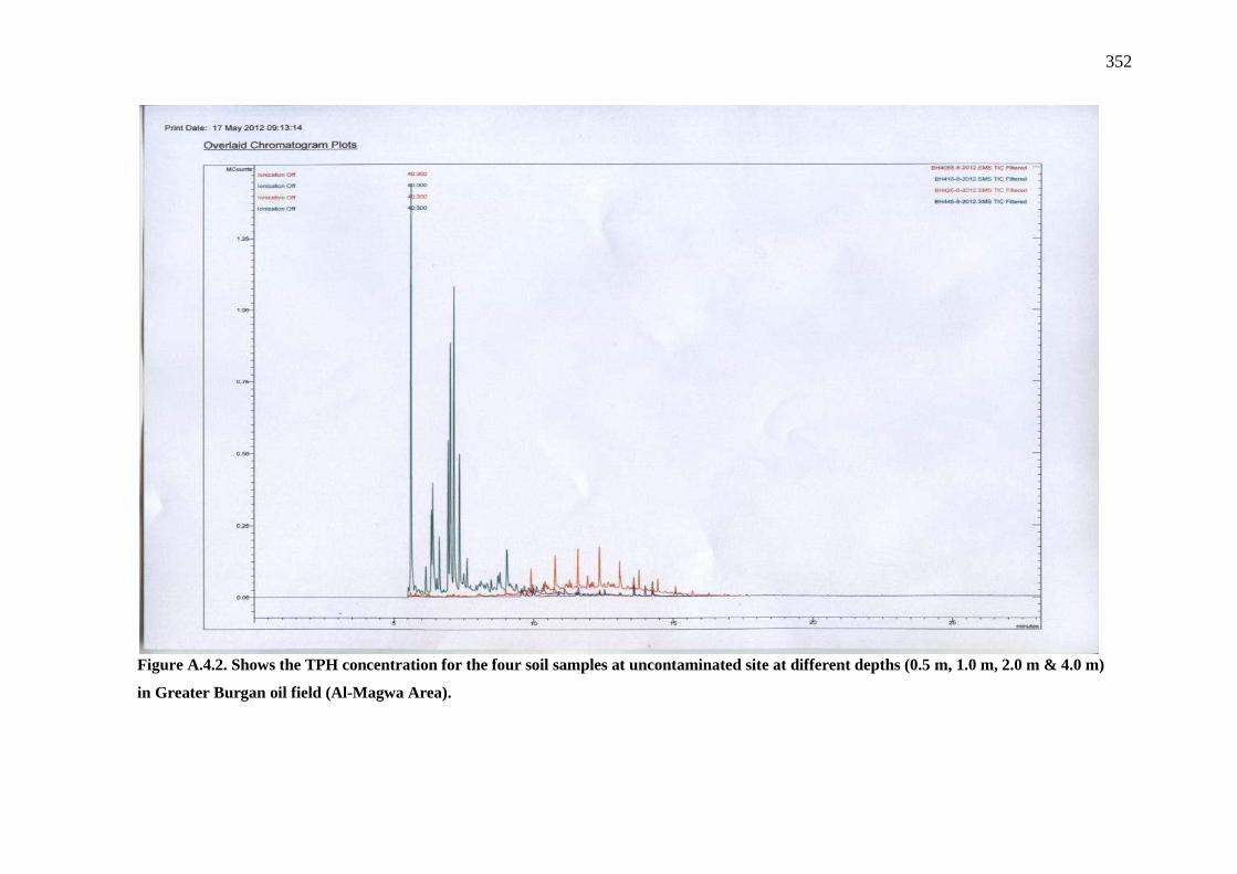
352
Figure A.4.2. Shows the TPH concentration for the four soil samples at uncontaminated site at different depths (0.5 m, 1.0 m, 2.0 m & 4.0 m)
in Greater Burgan oil field (Al-Magwa Area).
353
Figure A.4.3a. Shows the confidentially agreement between Kuwait Oil Company (KOC) and
University of Portsmouth.
354
Figure A.4.3b. Shows the confidentially agreement between Kuwait Oil Company (KOC) and
University of Portsmouth.

355
Figure A.4.3c. Shows the confidentially agreement between Kuwait Oil Company (KOC)
and University of Portsmouth.
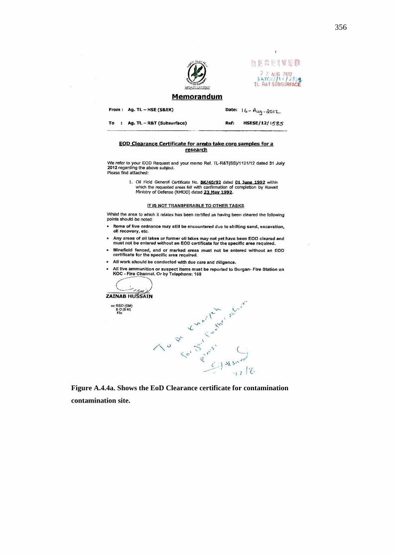
356
Figure A.4.4a. Shows the EoD Clearance certificate for contamination
contamination site.

357
Figure A.4.4b. Shows the EoD Clearance certificate for contamination contamination site.
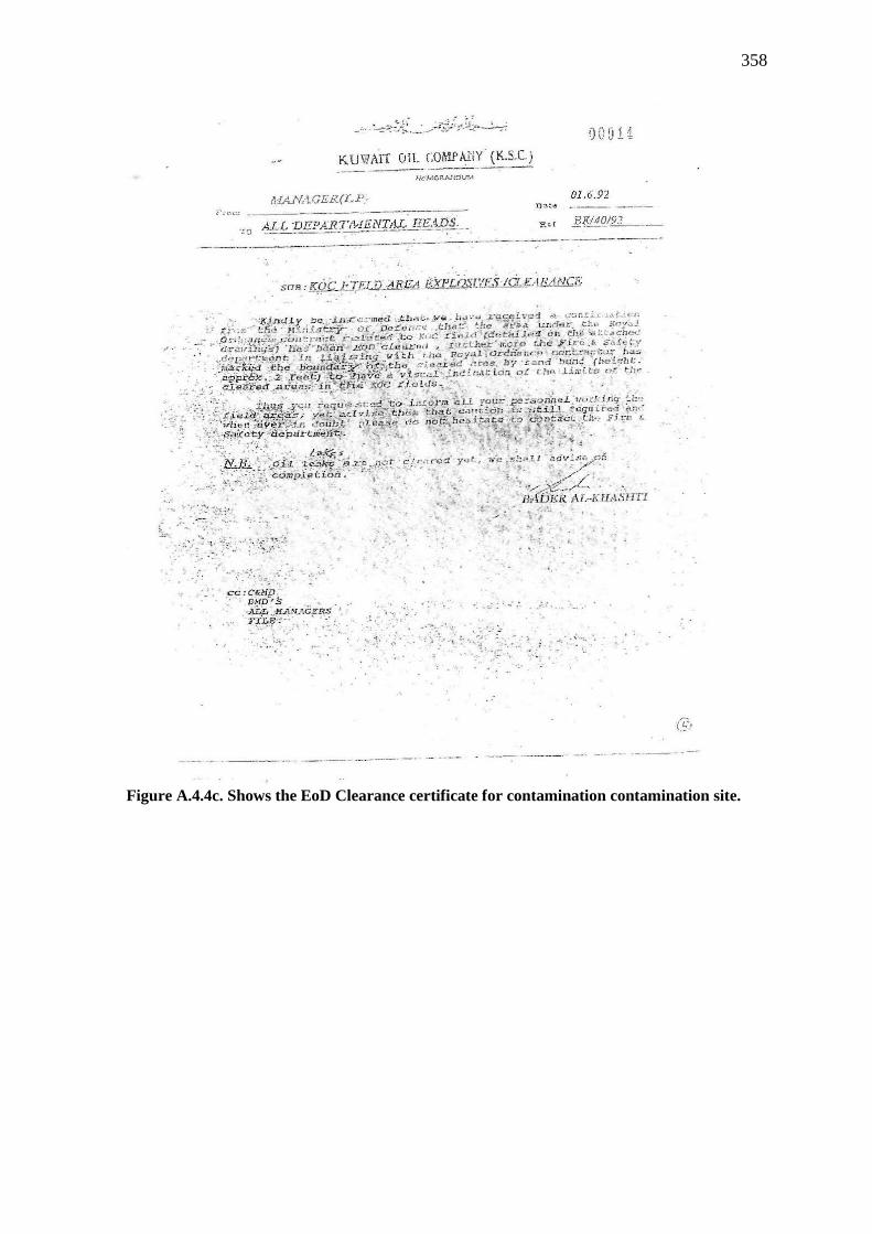
358
Figure A.4.4c. Shows the EoD Clearance certificate for contamination contamination site.

359
Figure A.4.4d. Shows the EoD Clearance certificate for contamination contamination site.
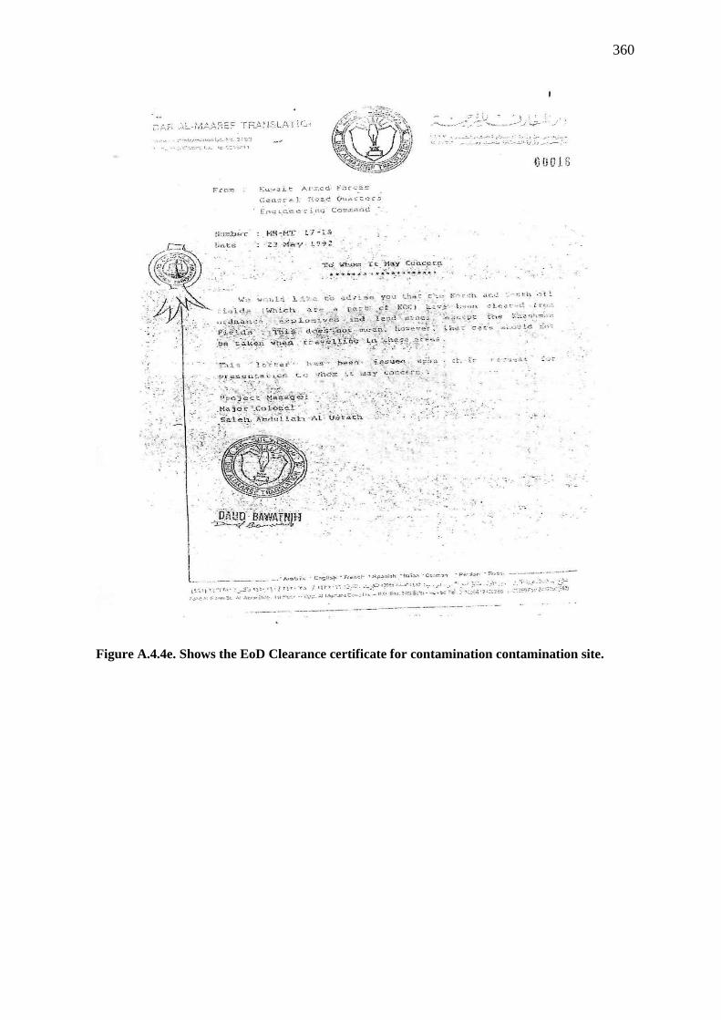
360
Figure A.4.4e. Shows the EoD Clearance certificate for contamination contamination site.
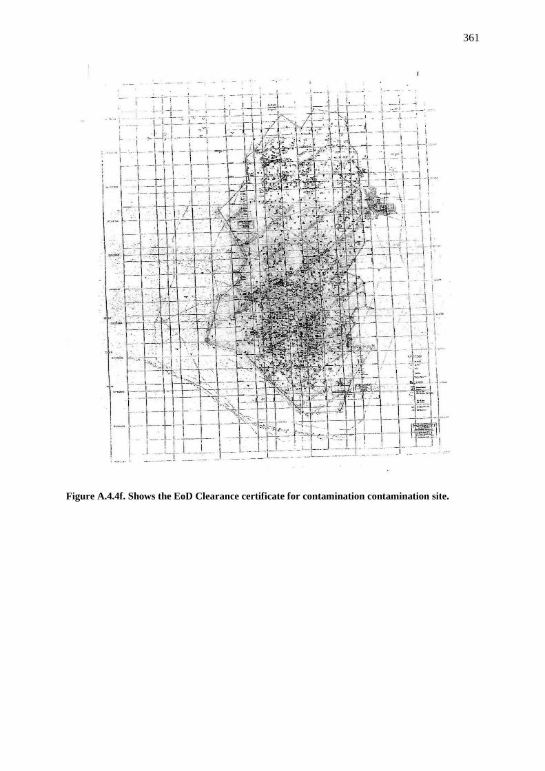
361
Figure A.4.4f. Shows the EoD Clearance certificate for contamination contamination site.

362
Figure A.4.5. Shows the the meeting one form with KOC expert staff concerning with sampling
project.

363
Figure A.4.6. Shows the the meeting two form with KOC expert staff concerning with
sampling project.

364
Figure A.4.7. Shows the temporary entry permit card.
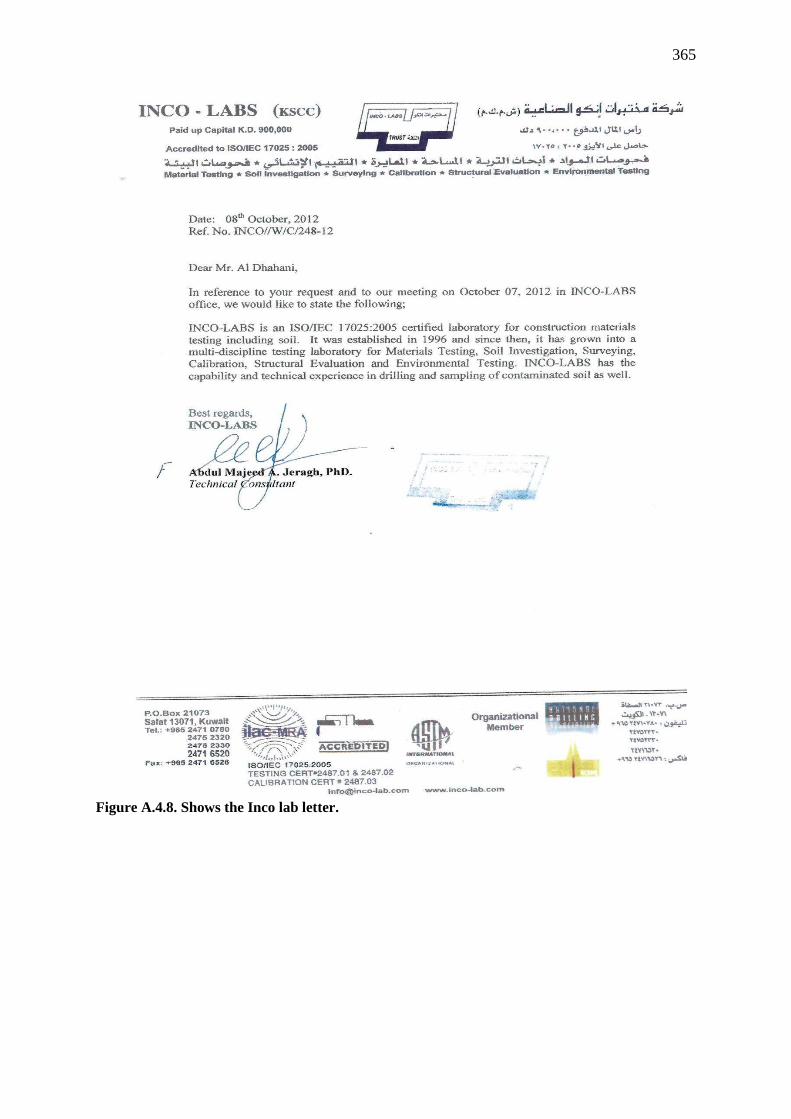
365
Figure A.4.8. Shows the Inco lab letter.
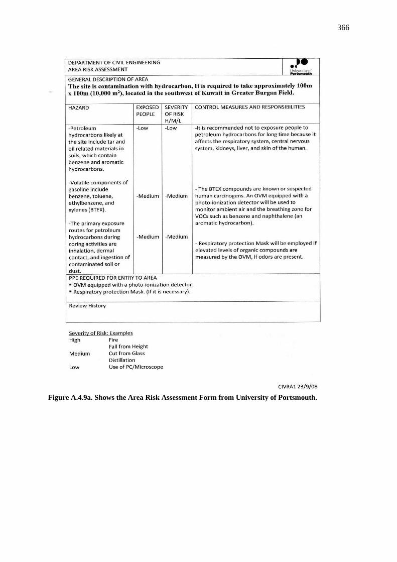
366
Figure A.4.9a. Shows the Area Risk Assessment Form from University of Portsmouth.

367
Figure A.4.9b. Shows the Area Risk Assessment Form from University of Portsmouth.

368
Figure A.4.9c. Shows the Area risk Assessment Form from University of Portsmouth.
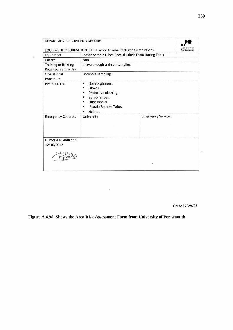
369
Figure A.4.9d. Shows the Area Risk Assessment Form from University of Portsmouth.

370
Figure A.4.10a. Shows the borehole log made by INCO company at the same study location
in Al- Magwa Area (INCO, 2007).
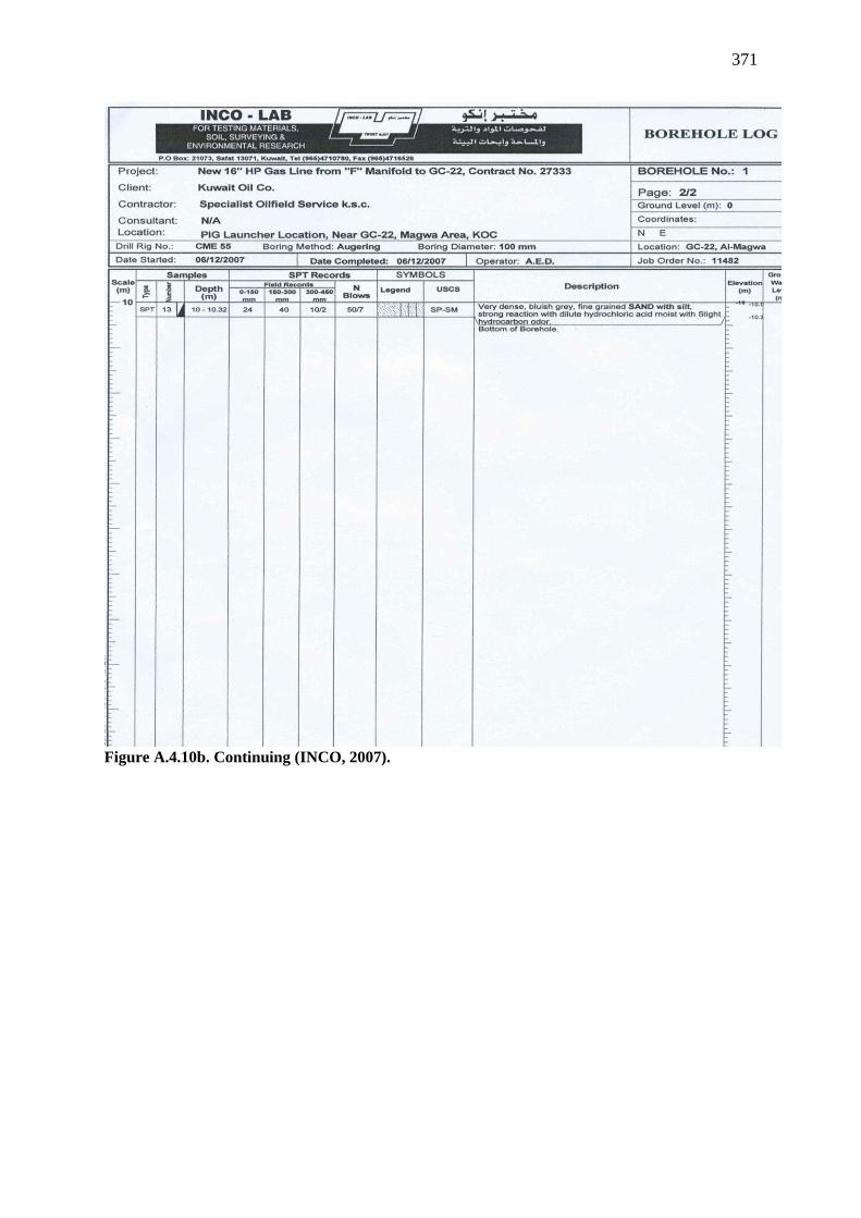
371
Figure A.4.10b. Continuing (INCO, 2007).

372
Figure A.4.11. Shows permitting card for the researcher from KOC in order to collect the main
soil samples from Greater Burgan field for the project.
Figure A.4.12. Shows my Kuwaiti Civil ID number which is matching with KOC passing gate
card for the Greater Burgan oil field (Al-Magwa Area).
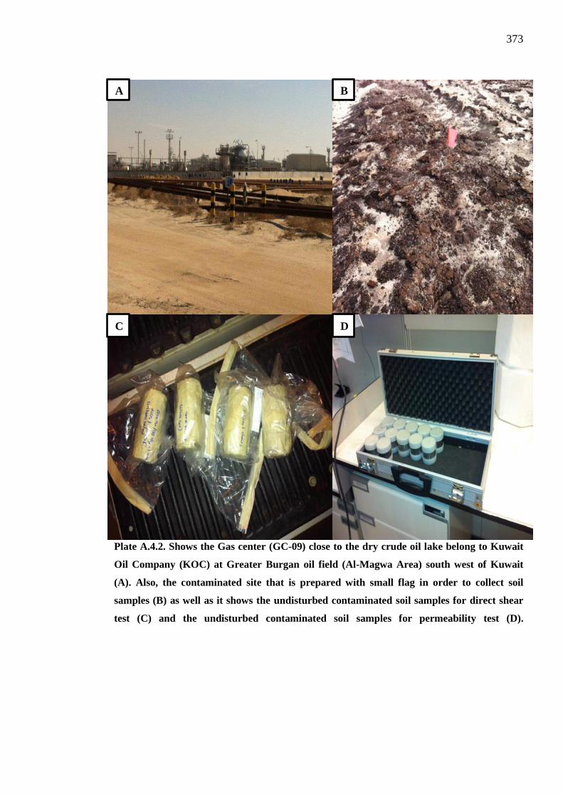
373
Plate A.4.2. Shows the Gas center (GC-09) close to the dry crude oil lake belong to Kuwait
Oil Company (KOC) at Greater Burgan oil field (Al-Magwa Area) south west of Kuwait
(A). Also, the contaminated site that is prepared with small flag in order to collect soil
samples (B) as well as it shows the undisturbed contaminated soil samples for direct shear
test (C) and the undisturbed contaminated soil samples for permeability test (D).
A B
C D

374
Figure A.4.13. Shows a letter from KISR and SMATCO labs concerning with samples
testing.
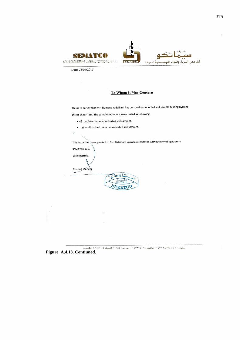
375
Figure A.4.13. Contiuned.

376
Figure A.4.14. The test of Liquid Limit: (a) liquid limit device; (b) grooving tool; (c) soil
pat before test; (d) soil pat after test. (Das, 2002).
Figure A.4.15. Plastic Limit test: (1) equipment; (2) beginning of test; (3) thread being
rolled; (4) crumbled soil. (Das, 2002).
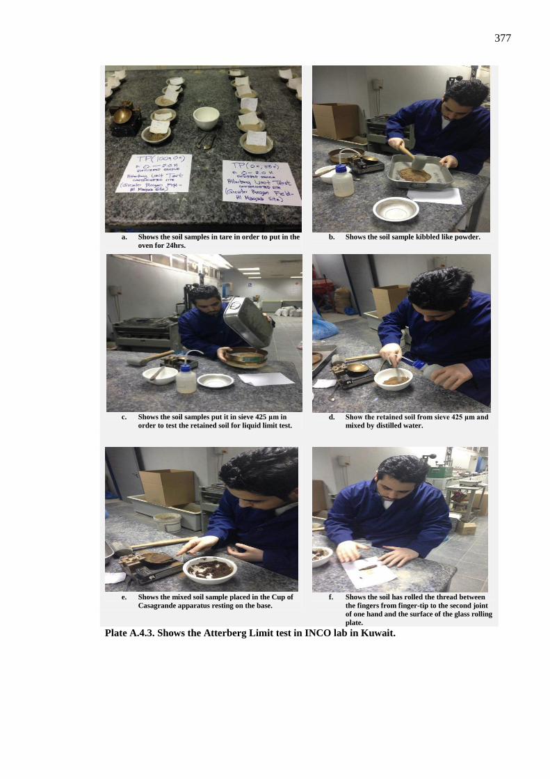
377
a. Shows the soil samples in tare in order to put in the
oven for 24hrs.
b. Shows the soil sample kibbled like powder.
c. Shows the soil samples put it in sieve 425 μm in
order to test the retained soil for liquid limit test.
d. Show the retained soil from sieve 425 μm and
mixed by distilled water.
e. Shows the mixed soil sample placed in the Cup of
Casagrande apparatus resting on the base.
f. Shows the soil has rolled the thread between
the fingers from finger-tip to the second joint of one hand and the surface of the glass rolling plate.
Plate A.4.3. Shows the Atterberg Limit test in INCO lab in Kuwait.

378
Figure A.4.16. Shows the Particles Size Distribution (PSD) curve for soil classification (BS-
1377-part 2, 1990).
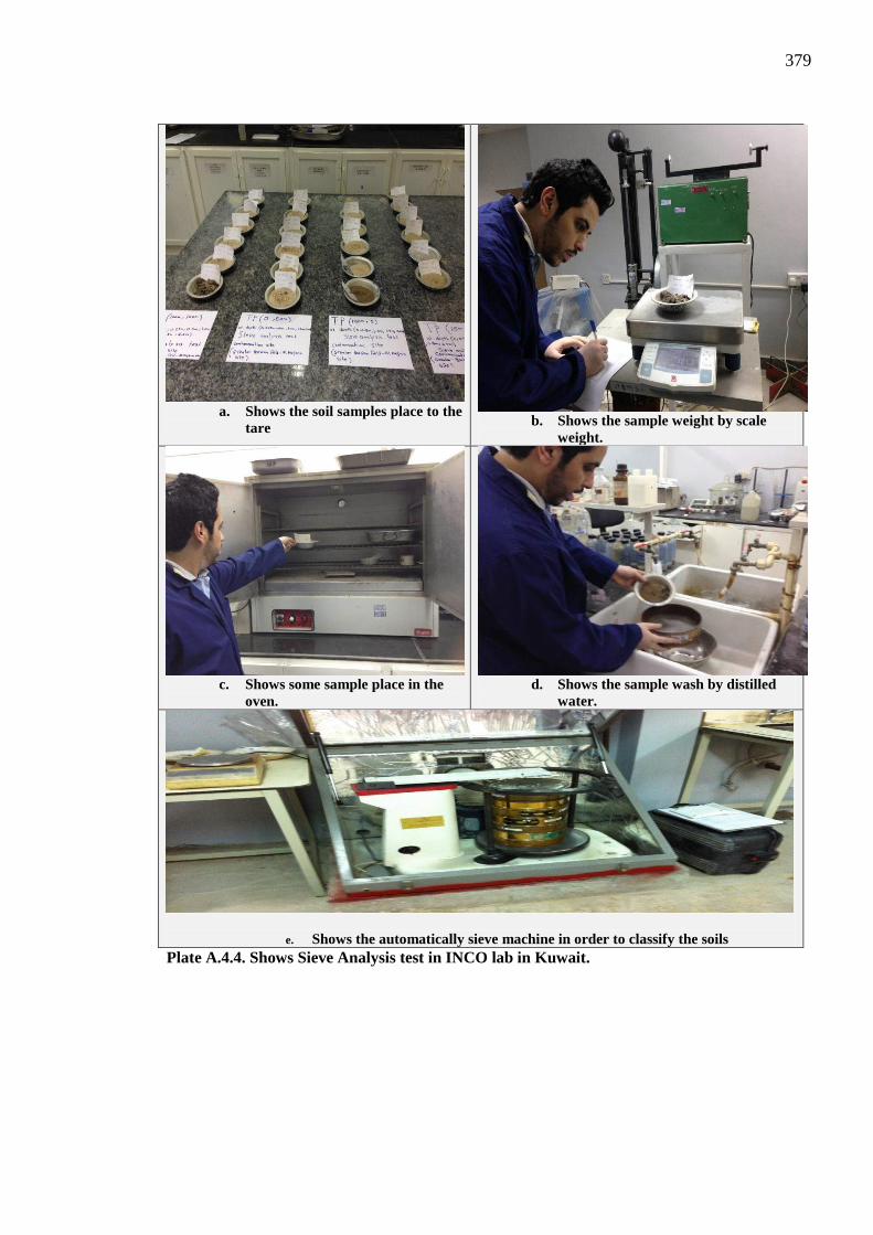
379
a. Shows the soil samples place to the
tare
b. Shows the sample weight by scale weight.
c. Shows some sample place in the
oven.
d. Shows the sample wash by distilled
water.
e. Shows the automatically sieve machine in order to classify the soils
Plate A.4.4. Shows Sieve Analysis test in INCO lab in Kuwait.
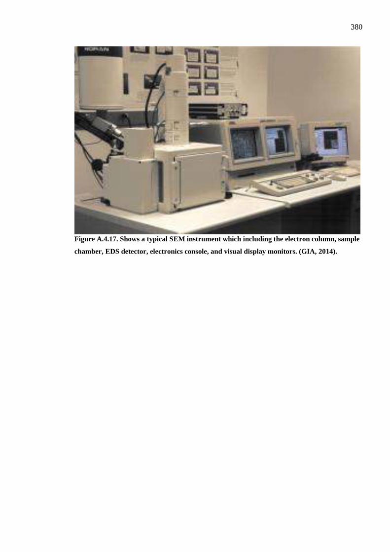
380
Figure A.4.17. Shows a typical SEM instrument which including the electron column, sample
chamber, EDS detector, electronics console, and visual display monitors. (GIA, 2014).

381
Table A.4.3. Shows the Permeability test (constant head method) procedures in accordance
with International Organization for Standardization-Part 11 (ISO/TS 17892-11: 2013).
Permeability Test
Procedures Numbers (No.)
Permeability Test (constant head method) in Accordance with BS 1377-5:1990
1 Placing the ring samples in the ring holders.
2 Allow the water to fill the permeater container. 3 Wait until the water level inside the sample container and water bath
reach the same level. 4 Place the bridge in sample holder to lower the water in the sample.
5 Wait until the water start to pass throw burret. 6 With help of Burret measure volume of the water passing throw the
sample in certain time. 7 Determine constant head with help of water level indicator for each
sample. 8 8-Insert all observe parameter such as (v), (L), (A), (t) & (h) in the
following equation.
The following equation was used to determine coefficient of permeability following
constant head method:
V x L
K=
A x t x h
Whereas
K= coefficient of permeability,
V= volume of water,
L= length of soil sample,
A= cross-section surface of the sample,
t = time,
h= calculate with the water levels measured with the water level meter.

382
a. Collected soil samples in sampling rings.
b. Eijkelkamp permeameter apparatus.
c. Soil samples the permeameter during testing.
d. Measurement of volume of water during testing.
Plate A.4.5. Shows the Permeability lab in Kuwait Institution Scientific Research (KISR) at
Shuwaikh-branch.

383
a. Showed the soil sample was tamped in the shear box (60mm square X 20 thick).
b. Shows the shear box placed in the carriage in order to apply the vertical and horizontal forces.
c. The Vertical load is applied and the horizontal gauge displacement is set.
d. Showed the reading of the vertical forces and displacement.
Plate A.4.6. Shows the Direct Shear test in SAMTCO lab in Kuwait.

384
a. Shows the 30g weight of dry soil
sample by scale weight.
b. Shows the 75mL of distilled water.
c. Shows the distil water mixing with
dry soil sample.
d. Shows the reading of pH meter.
Plate A.4.7. Shows the pH test in INCO lab in Kuwait.
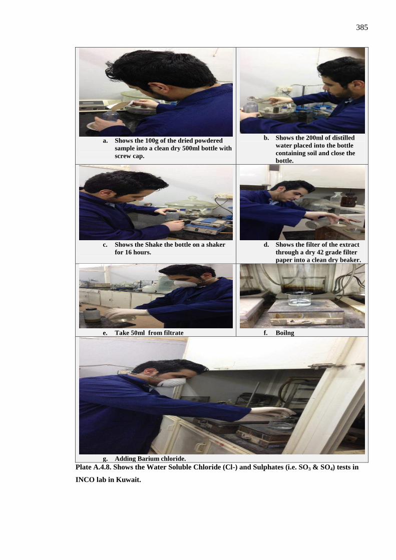
385
a. Shows the 100g of the dried powdered
sample into a clean dry 500ml bottle with screw cap.
b. Shows the 200ml of distilled
water placed into the bottle containing soil and close the bottle.
c. Shows the Shake the bottle on a shaker
for 16 hours.
d. Shows the filter of the extract
through a dry 42 grade filter paper into a clean dry beaker.
e. Take 50ml from filtrate
f. Boilng
g. Adding Barium chloride.
Plate A.4.8. Shows the Water Soluble Chloride (Cl-) and Sulphates (i.e. SO3 & SO4) tests in
INCO lab in Kuwait.
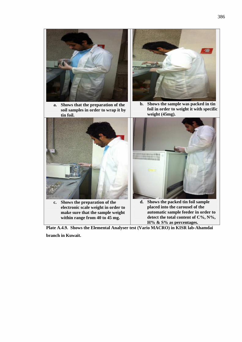
386
a. Shows that the preparation of the
soil samples in order to wrap it by tin foil.
b. Shows the sample was packed in tin
foil in order to weight it with specific weight (45mg).
c. Shows the preparation of the
electronic scale weight in order to make sure that the sample weight within range from 40 to 45 mg.
d. Shows the packed tin foil sample
placed into the carousel of the automatic sample feeder in order to detect the total content of C%, N%, H% & S% as percentages.
Plate A.4.9. Shows the Elemental Analyser test (Vario MACRO) in KISR lab-Ahamdai
branch in Kuwait.
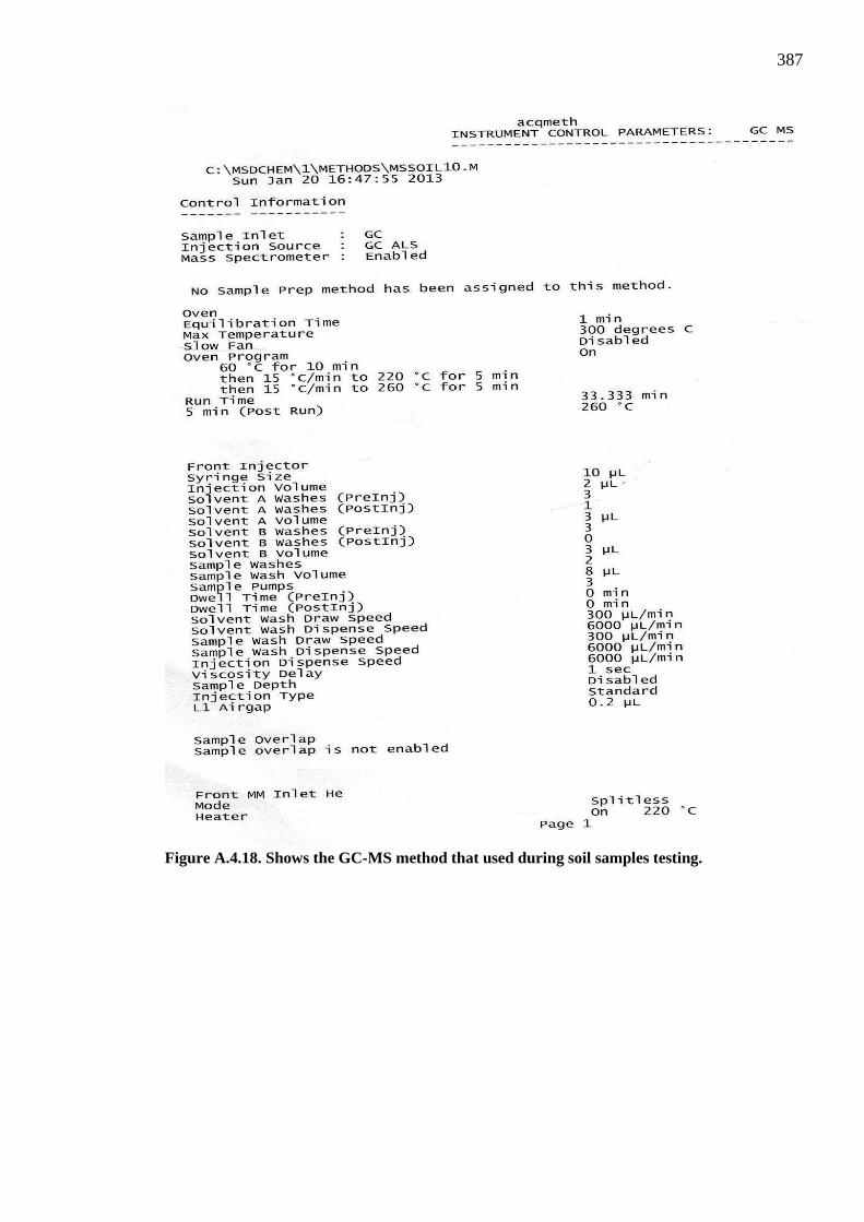
387
Figure A.4.18. Shows the GC-MS method that used during soil samples testing.
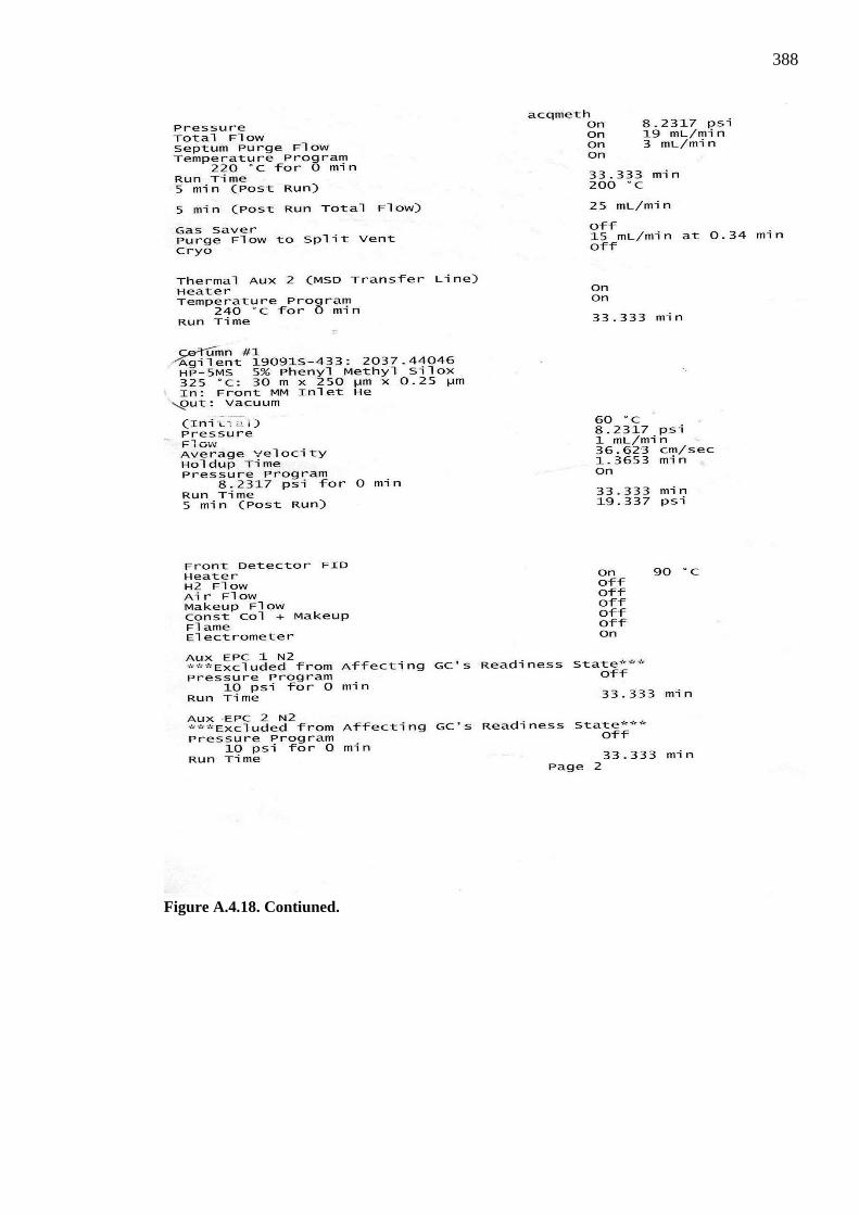
388
Figure A.4.18. Contiuned.

389
Figure A.4.18. Contiuned.
390
Figure A.4.18. Contiuned.

391
Figure A.4.18. Contiuned.

392
APPENDIX B
5. GEOTECHNICAL CHARACTERISATION. Particle Size Distribution (PSD)
At Depth (0.25 m)
At Depth (1.0 m)
At Depth (1.5 m)
Figure B.5.1. Shows the PSD Curves for contaminated samples at depths (0.25 m, 1.0 m &
1.5 m).
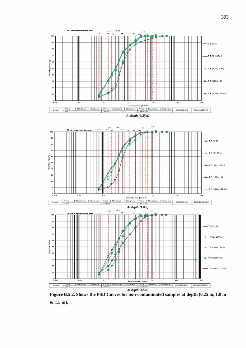
393
At depth (0.25m)
At depth (1.0m)
At depth (1.5m)
Figure B.5.2. Shows the PSD Curves for non-contaminated samples at depth (0.25 m, 1.0 m
& 1.5 m).

394
Table B.5.1. Shows the soil description results for contaminated samples at depth (0.0 m) in Greater Burgan oil field (Al-Magwa Area).
Trial Pits Coordinates. (T.P.Cs)
Proportions of Soil Class Percent (%) Silty/clay Passing
Percentages % (B.S. SIEVE No.#230)
Soil Classification Silty/Clay% Fine
Sand % Medium
Sand %
Coarse Sand
%
Gravel %
(0 m, 0 m) 11 7 34 22 15 11.3 Silty sand (S-M) (25 m, 0 m) 8 10 34 26 14 7.8 Silty sand (S-M) (50 m, 0 m) 5 51 24 11 4 5.0 Sand (SP) (75 m, 0 m) 16 25 23 15 5 16.4 Very silty Sand (S-M) (100 m, 0 m) 11 10 27 28 14 10.6 Silty Sand (S-M) (0 m , 25m) 5 24 39 25 2 5.2 Silty sand (S-M) (25 m, 25 m) 11 31 30 14 3 10.9 Silty sand (S-M) (50 m, 25 m) 15 28 21 12 9 15.2 Very silty sand (SM) (100 m, 25 m) 16 35 20 12 1 16.2 Very Silty Sand (S-M) (0 m, 50 m) 13 28 20 17 9 12.8 Silty sand (S-M) (25 m, 50 m) 15 28 20 11 11 15.2 Very silty sand (SM) (50 m, 50 m) 7 38 33 11 4 7.4 Silty Sand (S-M) (100 m, 50 m) 8 29 36 19 0 8 Silty Sand (S-M) (0 m, 75 m) 9 14 37 26 5 9.5 Silty Sand (S-M) (25 m, 75 m) 11 35 24 18 1 11.4 Silty sand (S-M) (50 m, 75 m) 12 54 13 9 1 11.9 Silty Sand (S-M) (75 m, 75 m) 10 42 25 12 1 10.3 Silty sand (S-M) (100 m, 75 m) 13 30 30 13 1 13.5 Silty Sand (S-M) (0 m, 100 m) 1 1 4 9 83 1.5 Sand (SP) (50 m, 100 m) 9 35 25 14 8 9 Silty sand (S-M) (75 m, 100 m) 8 31 32 20 1 8.3 Silty Sand (S-M) (100 m,100 m) 3 17 17 12 49 2.7 Sand (SP)
Min. Value 1 1 4 9 1 2.7 ------- Max. Value 16 54 39 28 83 16.4 ------- Mean Value 10 28 25 17 11 9.7 Silty Sand (S-M)
Standard Deviation Value 4.08 13.49 8.51 5.95 19.16 4.11 -------
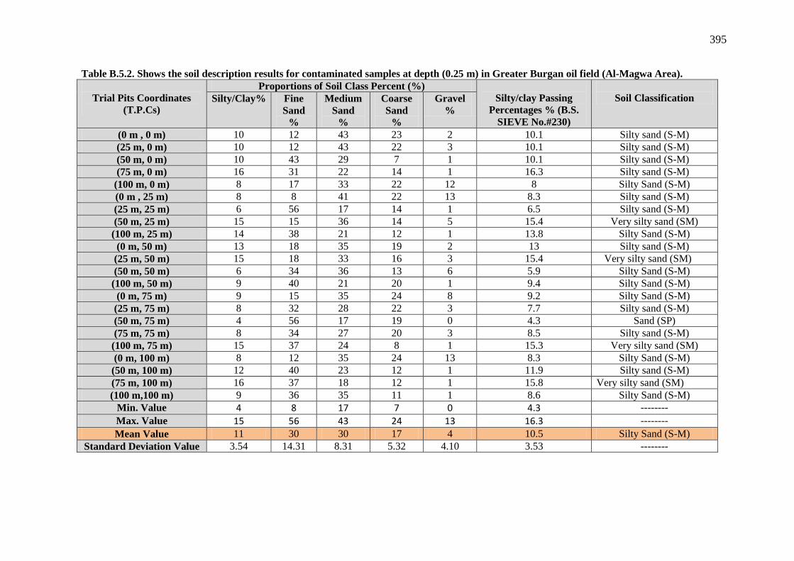
395
Table B.5.2. Shows the soil description results for contaminated samples at depth (0.25 m) in Greater Burgan oil field (Al-Magwa Area).
Trial Pits Coordinates (T.P.Cs)
Proportions of Soil Class Percent (%) Silty/clay Passing
Percentages % (B.S. SIEVE No.#230)
Soil Classification Silty/Clay% Fine
Sand %
Medium Sand
%
Coarse Sand
%
Gravel %
(0 m , 0 m) 10 12 43 23 2 10.1 Silty sand (S-M) (25 m, 0 m) 10 12 43 22 3 10.1 Silty sand (S-M) (50 m, 0 m) 10 43 29 7 1 10.1 Silty sand (S-M) (75 m, 0 m) 16 31 22 14 1 16.3 Silty sand (S-M)
(100 m, 0 m) 8 17 33 22 12 8 Silty Sand (S-M) (0 m , 25 m) 8 8 41 22 13 8.3 Silty sand (S-M) (25 m, 25 m) 6 56 17 14 1 6.5 Silty sand (S-M) (50 m, 25 m) 15 15 36 14 5 15.4 Very silty sand (SM)
(100 m, 25 m) 14 38 21 12 1 13.8 Silty Sand (S-M) (0 m, 50 m) 13 18 35 19 2 13 Silty sand (S-M)
(25 m, 50 m) 15 18 33 16 3 15.4 Very silty sand (SM) (50 m, 50 m) 6 34 36 13 6 5.9 Silty Sand (S-M)
(100 m, 50 m) 9 40 21 20 1 9.4 Silty Sand (S-M) (0 m, 75 m) 9 15 35 24 8 9.2 Silty Sand (S-M)
(25 m, 75 m) 8 32 28 22 3 7.7 Silty sand (S-M) (50 m, 75 m) 4 56 17 19 0 4.3 Sand (SP) (75 m, 75 m) 8 34 27 20 3 8.5 Silty sand (S-M)
(100 m, 75 m) 15 37 24 8 1 15.3 Very silty sand (SM) (0 m, 100 m) 8 12 35 24 13 8.3 Silty Sand (S-M)
(50 m, 100 m) 12 40 23 12 1 11.9 Silty sand (S-M) (75 m, 100 m) 16 37 18 12 1 15.8 Very silty sand (SM) (100 m,100 m) 9 36 35 11 1 8.6 Silty Sand (S-M)
Min. Value 4 8 17 7 0 4.3 -------- Max. Value 15 56 43 24 13 16.3 -------- Mean Value 11 30 30 17 4 10.5 Silty Sand (S-M)
Standard Deviation Value 3.54 14.31 8.31 5.32 4.10 3.53 --------
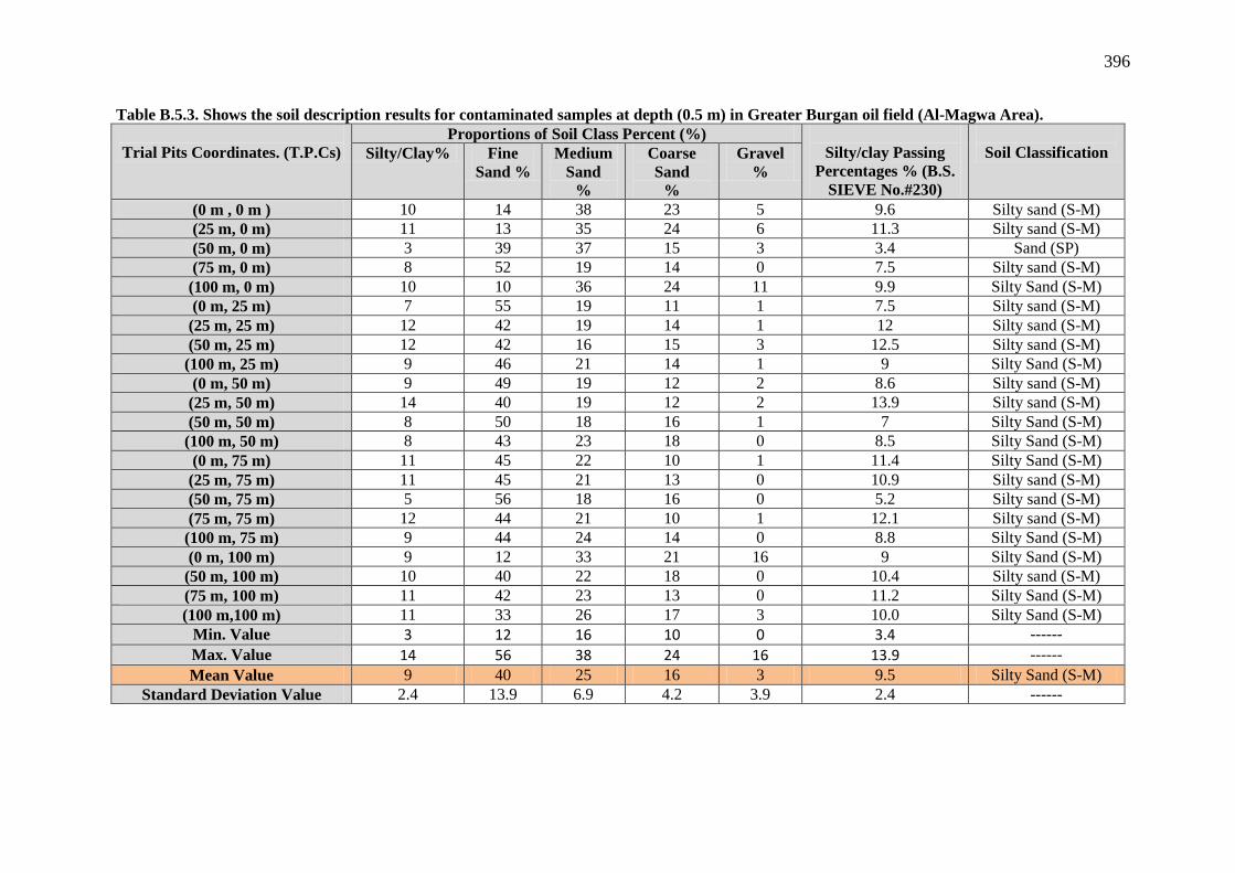
396
Table B.5.3. Shows the soil description results for contaminated samples at depth (0.5 m) in Greater Burgan oil field (Al-Magwa Area).
Trial Pits Coordinates. (T.P.Cs) Proportions of Soil Class Percent (%)
Silty/clay Passing Percentages % (B.S.
SIEVE No.#230)
Soil Classification Silty/Clay% Fine
Sand % Medium
Sand %
Coarse Sand
%
Gravel %
(0 m , 0 m ) 10 14 38 23 5 9.6 Silty sand (S-M) (25 m, 0 m) 11 13 35 24 6 11.3 Silty sand (S-M) (50 m, 0 m) 3 39 37 15 3 3.4 Sand (SP) (75 m, 0 m) 8 52 19 14 0 7.5 Silty sand (S-M) (100 m, 0 m) 10 10 36 24 11 9.9 Silty Sand (S-M) (0 m, 25 m) 7 55 19 11 1 7.5 Silty sand (S-M) (25 m, 25 m) 12 42 19 14 1 12 Silty sand (S-M) (50 m, 25 m) 12 42 16 15 3 12.5 Silty sand (S-M) (100 m, 25 m) 9 46 21 14 1 9 Silty Sand (S-M) (0 m, 50 m) 9 49 19 12 2 8.6 Silty sand (S-M) (25 m, 50 m) 14 40 19 12 2 13.9 Silty sand (S-M) (50 m, 50 m) 8 50 18 16 1 7 Silty Sand (S-M) (100 m, 50 m) 8 43 23 18 0 8.5 Silty Sand (S-M) (0 m, 75 m) 11 45 22 10 1 11.4 Silty Sand (S-M) (25 m, 75 m) 11 45 21 13 0 10.9 Silty sand (S-M) (50 m, 75 m) 5 56 18 16 0 5.2 Silty sand (S-M) (75 m, 75 m) 12 44 21 10 1 12.1 Silty sand (S-M) (100 m, 75 m) 9 44 24 14 0 8.8 Silty Sand (S-M) (0 m, 100 m) 9 12 33 21 16 9 Silty Sand (S-M) (50 m, 100 m) 10 40 22 18 0 10.4 Silty sand (S-M) (75 m, 100 m) 11 42 23 13 0 11.2 Silty Sand (S-M) (100 m,100 m) 11 33 26 17 3 10.0 Silty Sand (S-M)
Min. Value 3 12 16 10 0 3.4 ------ Max. Value 14 56 38 24 16 13.9 ------ Mean Value 9 40 25 16 3 9.5 Silty Sand (S-M)
Standard Deviation Value 2.4 13.9 6.9 4.2 3.9 2.4 ------

397
Table B.5.4. Shows the soil description results for contaminated samples at depth (1.0 m) in Greater Burgan oil field (Al-Magwa Area).
Trial Pits Coordinates. (T.P.Cs)
Proportions of Soil Class Percent (%) Silty/clay Passing
Percentages % (B.S. SIEVE No.#230)
Soil Classification Silty/Clay% Fine
Sand % Medium
Sand %
Coarse Sand
%
Gravel %
(0 m , 0 m) 13 14 35 20 5 12.8 Silty sand (S-M) (25 m, 0 m) 13 14 33 22 5 13.0 Silty sand (S-M) (50 m, 0 m) 6 48 26 12 2 5.7 Silty sand (S-M) (75 m, 0 m) 5 59 18 13 0 4.9 Sand (SP)
(100 m, 0 m) 11 44 20 12 2 11.4 Silty Sand (S-M) (0 m, 25 m) 7 60 18 8 0 7 Silty sand (S-M)
(25 m, 25 m) 6 58 19 11 0 6 Silty sand (S-M) (50 m, 25 m) 12 41 21 12 2 12.4 Silty sand (S-M) (100 m, 25 m) 5 61 17 12 0 5.2 Silty Sand (S-M)
(0 m, 50 m) 8 53 18 12 1 7.8 Silty sand (S-M) (25 m, 50 m) 12 44 20 9 3 12.1 Silty sand (S-M) (50 m, 50 m) 9 51 19 12 0 9.2 Silty Sand (S-M) (100 m, 50 m) 7 49 19 18 0 7 Silty Sand (S-M)
(0 m, 75 m) 5 62 17 12 0 4.6 Sand (SP) (25 m, 75 m) 5 60 17 14 0 4.9 Sand (SP) (50 m, 75 m) 10 42 26 12 0 10.3 Silty sand (S-M) (75 m, 75 m) 7 56 18 13 0 6.7 Silty sand (S-M) (100 m, 75 m) 8 54 17 14 0 7.6 Silty Sand (S-M) (0 m, 100 m) 6 36 24 13 15 6.2 Silty Sand (S-M) (50 m, 100 m) 5 55 18 17 0 5.1 Silty sand (S-M) (75 m, 100 m) 8 52 18 15 0 7.6 Silty Sand (S-M) (100 m,100 m) 6 39 30 19 0 5.6 Silty Sand (S-M)
Min. Value 5 14 17 8 0 4.6 ------ Max. Value 13 62 35 22 15 12.8 ------ Mean Value 8 49 21 14 2 7.9 Silty Sand (S-M)
Standard Deviation Value 2.7 13.3 5.39 3.48 1.59 2.8 ------

398
Table B.5.5. Shows the soil description results for contaminated samples at depth (1.5 m) in Greater Burgan oil field (Al-Magwa Area).
Trial Pits Coordinates (T.P.Cs)
Proportions of Soil Class Percent (%) Silty/clay Passing Percentages % (B.S.
SIEVE No.#230)
Soil Classification Silty/Clay% Fine
Sand %
Medium Sand
%
Coarse Sand
%
Gravel %
(0 m, 0 m) 8 28 28 23 6 7.9 Silty sand (S-M) (25 m, 0 m) 9 18 25 31 8 9 Silty sand (S-M) (50 m, 0 m) 5 45 27 17 1 4.7 Sand (SP) (75 m, 0 m) 4 56 17 19 0 4.1 Sand (SP) (100 m, 0 m) 6 56 22 10 0 6.4 Silty Sand (S-M) (0 m, 25 m) 3 60 17 18 0 2.7 Sand (SP) (25 m, 25 m) 3 61 16 17 0 3.1 Sand (SP) (50 m, 25 m) 12 51 14 10 1 12.4 Silty sand (S-M)
(100 m, 25 m) 4 62 16 13 1 3.8 Sand (SP) (0 m, 50 m) 5 62 15 13 0 5.4 Silty sand (S-M) (25 m, 50 m) 13 47 14 12 0 13.2 Silty sand (S-M) (50 m, 50 m) 10 51 17 11 1 10 Silty Sand (S-M)
(100 m, 50 m) 10 42 18 20 1 9.6 Silty Sand (S-M) (0 m, 75 m) 4 62 16 15 0 3.6 Sand (SP) (25 m, 75 m) 5 59 15 17 0 4.6 Sand (SP) (50 m, 75 m) 8 48 22 13 1 8.4 Silty sand (S-M) (75 m, 75 m) 8 57 17 11 0 7.5 Silty sand (S-M) (100 m, 75m) 16 26 18 21 3 16.1 Very silty sand (SM) (0 m, 100 m) 7 24 32 20 11 6.7 Silty Sand (S-M)
(50 m, 100 m) 11 30 21 21 6 10.9 Silty sand (S-M) (75 m, 100 m) 16 24 18 23 3 16 Very Silty Sand (SM) (100 m,100 m) 5 27 23 24 16 5.3 Silty Sand (S-M)
Min. Value 3 18 14 10 0 2.7 ------ Max. Value 16 62 32 31 16 16.1 ------ Mean Value 8 45 20 17 3 7.8 Silty Sand (S-M)
Standard Deviation Value 3.9 15.1 4.9 5.4 4.2 4.0 ------
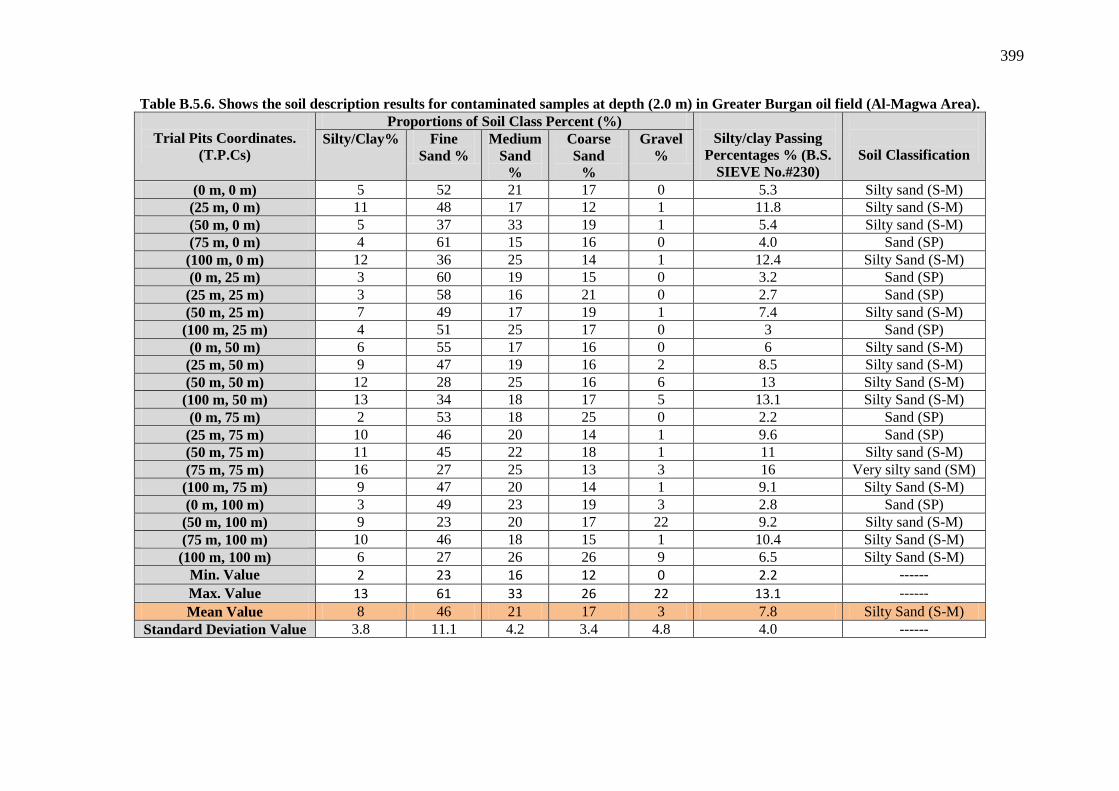
399
Table B.5.6. Shows the soil description results for contaminated samples at depth (2.0 m) in Greater Burgan oil field (Al-Magwa Area).
Trial Pits Coordinates. (T.P.Cs)
Proportions of Soil Class Percent (%) Silty/clay Passing
Percentages % (B.S. SIEVE No.#230)
Soil Classification Silty/Clay% Fine
Sand % Medium
Sand %
Coarse Sand
%
Gravel %
(0 m, 0 m) 5 52 21 17 0 5.3 Silty sand (S-M) (25 m, 0 m) 11 48 17 12 1 11.8 Silty sand (S-M) (50 m, 0 m) 5 37 33 19 1 5.4 Silty sand (S-M) (75 m, 0 m) 4 61 15 16 0 4.0 Sand (SP)
(100 m, 0 m) 12 36 25 14 1 12.4 Silty Sand (S-M) (0 m, 25 m) 3 60 19 15 0 3.2 Sand (SP)
(25 m, 25 m) 3 58 16 21 0 2.7 Sand (SP) (50 m, 25 m) 7 49 17 19 1 7.4 Silty sand (S-M) (100 m, 25 m) 4 51 25 17 0 3 Sand (SP)
(0 m, 50 m) 6 55 17 16 0 6 Silty sand (S-M) (25 m, 50 m) 9 47 19 16 2 8.5 Silty sand (S-M) (50 m, 50 m) 12 28 25 16 6 13 Silty Sand (S-M) (100 m, 50 m) 13 34 18 17 5 13.1 Silty Sand (S-M)
(0 m, 75 m) 2 53 18 25 0 2.2 Sand (SP) (25 m, 75 m) 10 46 20 14 1 9.6 Sand (SP) (50 m, 75 m) 11 45 22 18 1 11 Silty sand (S-M) (75 m, 75 m) 16 27 25 13 3 16 Very silty sand (SM) (100 m, 75 m) 9 47 20 14 1 9.1 Silty Sand (S-M) (0 m, 100 m) 3 49 23 19 3 2.8 Sand (SP) (50 m, 100 m) 9 23 20 17 22 9.2 Silty sand (S-M) (75 m, 100 m) 10 46 18 15 1 10.4 Silty Sand (S-M)
(100 m, 100 m) 6 27 26 26 9 6.5 Silty Sand (S-M) Min. Value 2 23 16 12 0 2.2 ------ Max. Value 13 61 33 26 22 13.1 ------ Mean Value 8 46 21 17 3 7.8 Silty Sand (S-M)
Standard Deviation Value 3.8 11.1 4.2 3.4 4.8 4.0 ------
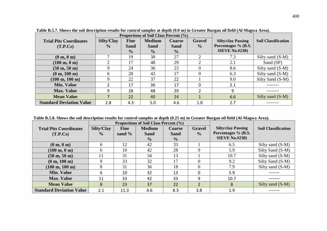
400
Table B.5.7. Shows the soil description results for control samples at depth (0.0 m) in Greater Burgan oil field (Al-Magwa Area).
Trial Pits Coordinates (T.P.Cs)
Proportions of Soil Class Percent (%) Silty/clay Passing
Percentages % (B.S. SIEVE No.#230)
Soil Classification Silty/Clay
% Fine Sand
%
Medium Sand
%
Coarse Sand
%
Gravel %
(0 m, 0 m) 7 19 38 27 2 7.3 Silty sand (S-M) (100 m, 0 m) 2 17 48 29 2 2.1 Sand (SP) (50 m, 50 m) 9 24 36 23 0 8.6 Silty sand (S-M) (0 m, 100 m) 6 28 43 17 0 6.3 Silty sand (S-M)
(100 m, 100 m) 9 22 37 22 1 9.0 Silty Sand (S-M) Min. Value 2 17 36 17 0 2.1 -------- Max. Value 9 28 48 29 2 9 -------- Mean Value 7 22 40 24 1 6.6 Silty sand (S-M)
Standard Deviation Value 2.8 4.3 5.0 4.6 1.0 2.7 --------
Table B.5.8. Shows the soil description results for control samples at depth (0.25 m) in Greater Burgan oil field (Al-Magwa Area).
Trial Pits Coordinates (T.P.Cs)
Proportions of Soil Class Percent (%) Silty/clay Passing
Percentages % (B.S. SIEVE No.#230)
Soil Classification Silty/Clay
% Fine
sand % Medium
Sand %
Coarse Sand
%
Gravel %
(0 m, 0 m) 6 12 42 33 1 6.5 Silty sand (S-M) (100 m, 0 m) 6 10 42 28 9 5.9 Silty Sand (S-M) (50 m, 50 m) 11 31 34 13 1 10.7 Silty sand (S-M) (0 m, 100 m) 9 33 32 17 0 9.2 Silty Sand (S-M)
(100 m, 100 m) 8 31 36 18 0 7.9 Silty sand (S-M) Min. Value 6 10 32 13 0 5.9 ------- Max. Value 11 33 42 33 9 10.7 ------- Mean Value 8 23 37 22 2 8 Silty sand (S-M)
Standard Deviation Value 2.1 11.3 4.6 8.3 3.8 1.9 -------

401
Table B.5.9. Shows the soil description results for control samples at depth (0.5 m) in Greater Burgan oil field (Al-Magwa Area).
Trial Pits Coordinates. (T.P.Cs)
Proportions of Soil Class Percent (%) Silty/clay Passing
Percentages % (B.S. SIEVE No.#230)
Soil Classification Silty/Clay
% Fine Sand
%
Medium Sand
%
Coarse Sand
%
Gravel %
(0 m, 0 m) 6 12 43 23 11 5.6 Silty sand (S-M) (100 m, 0 m) 5 20 45 22 3 5.3 Silty Sand (S-M) (50 m, 50 m) 11 30 32 17 0 10.6 Silty sand (S-M) (0 m, 100 m) 10 26 41 13 0 10.5 Silty sand (S-M)
(100 m, 100 m) 9 25 36 22 0 8.7 Silty Sand (S-M) Min. Value 5 12 32 13 0 5.3 ------- Max. Value 11 30 45 23 11 10.6 ------- Mean Value 8 23 39 20 3 8.2 Silty Sand (S-M)
Standard Deviation Value 2.5 6.9 5.3 4.2 4.7 2.5 -------
Table B.5.10. Shows the soil description results for control samples at depth (1.0 m) in Greater Burgan oil field (Al-Magwa Area).
Trial Pits Coordinates (T.P.Cs)
Proportions of Soil Class Percent (%) Silty/clay Passing
Percentages % (B.S. SIEVE No.#230)
Soil Classification Silty/Clay% Fine
Sand %
Medium Sand
%
Coarse Sand
%
Gravel %
(0 m , 0 m) 8 26 35 18 5 8.5 Silty sand (S-M) (100 m, 0 m) 6 9 43 35 1 6.1 Silty Sand (S-M) (50 m, 50 m) 7 36 33 18 0 6.6 Silty sand (S-M) (0 m, 100 m) 8 28 37 19 0 8.4 Silty sand (S-M)
(100 m, 100 m) 7 34 32 20 0 7.4 Silty Sand (S-M) Min. Value 6 9 32 18 0 6.1 ------- Max. Value 8 36 43 35 5 8.5 ------- Mean Value 7 26 36 22 1 7.4 Silty Sand (S-M)
Standard Deviation Value 0.8 10.6 4.3 7.3 2.1 1.0 -------
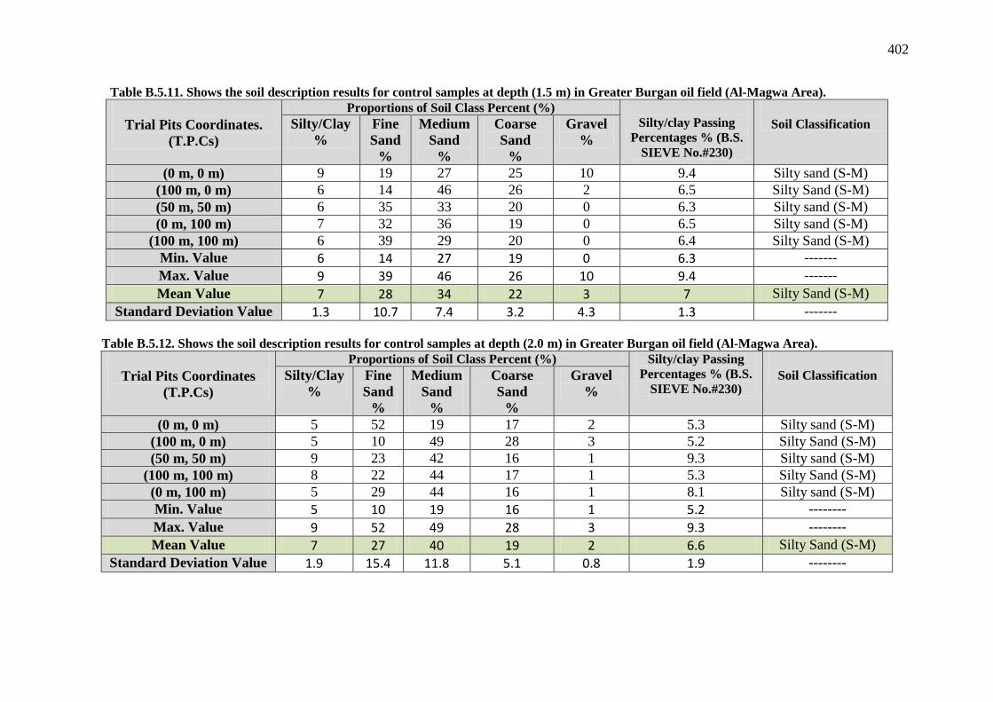
402
Table B.5.11. Shows the soil description results for control samples at depth (1.5 m) in Greater Burgan oil field (Al-Magwa Area).
Trial Pits Coordinates. (T.P.Cs)
Proportions of Soil Class Percent (%) Silty/clay Passing
Percentages % (B.S. SIEVE No.#230)
Soil Classification Silty/Clay
% Fine Sand
%
Medium Sand
%
Coarse Sand
%
Gravel %
(0 m, 0 m) 9 19 27 25 10 9.4 Silty sand (S-M) (100 m, 0 m) 6 14 46 26 2 6.5 Silty Sand (S-M) (50 m, 50 m) 6 35 33 20 0 6.3 Silty sand (S-M) (0 m, 100 m) 7 32 36 19 0 6.5 Silty sand (S-M)
(100 m, 100 m) 6 39 29 20 0 6.4 Silty Sand (S-M) Min. Value 6 14 27 19 0 6.3 ------- Max. Value 9 39 46 26 10 9.4 ------- Mean Value 7 28 34 22 3 7 Silty Sand (S-M)
Standard Deviation Value 1.3 10.7 7.4 3.2 4.3 1.3 -------
Table B.5.12. Shows the soil description results for control samples at depth (2.0 m) in Greater Burgan oil field (Al-Magwa Area).
Trial Pits Coordinates (T.P.Cs)
Proportions of Soil Class Percent (%) Silty/clay Passing Percentages % (B.S.
SIEVE No.#230)
Soil Classification Silty/Clay
% Fine Sand
%
Medium Sand
%
Coarse Sand
%
Gravel %
(0 m, 0 m) 5 52 19 17 2 5.3 Silty sand (S-M) (100 m, 0 m) 5 10 49 28 3 5.2 Silty Sand (S-M) (50 m, 50 m) 9 23 42 16 1 9.3 Silty sand (S-M)
(100 m, 100 m) 8 22 44 17 1 5.3 Silty Sand (S-M) (0 m, 100 m) 5 29 44 16 1 8.1 Silty sand (S-M) Min. Value 5 10 19 16 1 5.2 -------- Max. Value 9 52 49 28 3 9.3 -------- Mean Value 7 27 40 19 2 6.6 Silty Sand (S-M)
Standard Deviation Value 1.9 15.4 11.8 5.1 0.8 1.9 --------

403
Table B.5.13. The significant p-values via normality Shapiro-Wilk test indicate that the soil constituents data (i.e. silty/clay %, fine sand %, medium sand %, Coarse Sand % and exact soil passing No. 230) at contaminated and non-contaminated sites follow normal distribution.
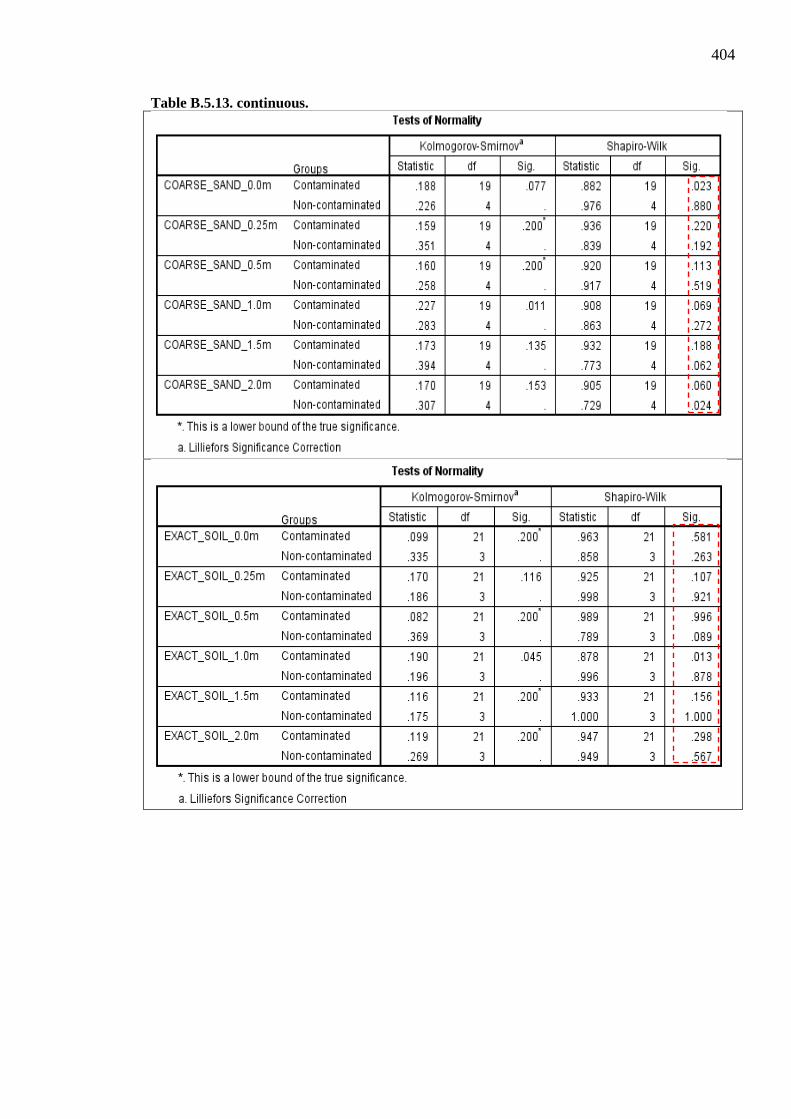
404
Table B.5.13. continuous.
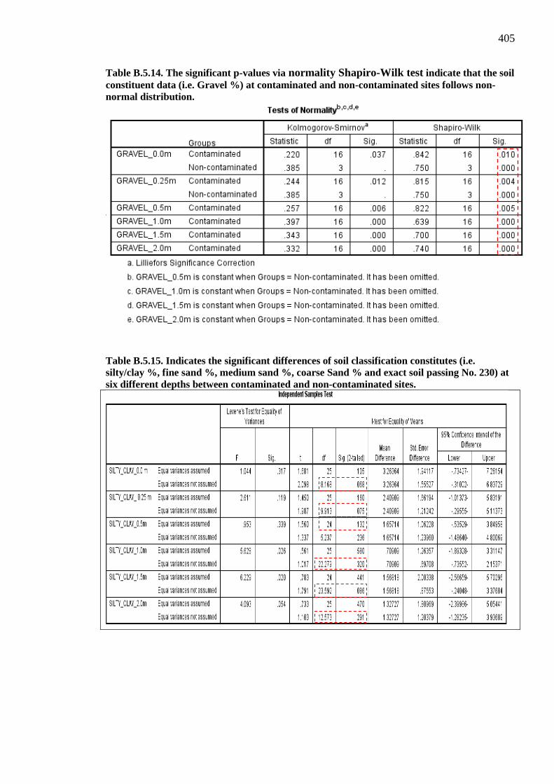
405
Table B.5.14. The significant p-values via normality Shapiro-Wilk test indicate that the soil constituent data (i.e. Gravel %) at contaminated and non-contaminated sites follows non-normal distribution.
Table B.5.15. Indicates the significant differences of soil classification constitutes (i.e. silty/clay %, fine sand %, medium sand %, coarse Sand % and exact soil passing No. 230) at six different depths between contaminated and non-contaminated sites.
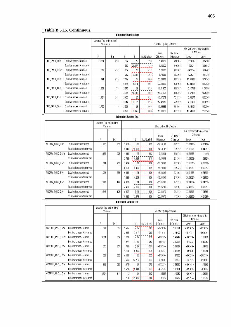
406
Table B.5.15. Continuous.

407
Table B.5.15. Continuous.
Table 5.16. Indicates the significant differences of soil classification constitutes (i.e. gravel) at six different depths between contaminated and non-contaminated sites.

408
Table B.5.17. The significant p-values via normality Shapiro-Wilk test indicate that the curvature coefficient (Cc) data of the soil classification at contaminated and non-contaminated sites follows normal distribution.
Table B.5.18. The significant p-values via normality Shapiro-Wilk test indicate that the uniformity coefficient (Cu) data of the soil classification at contaminated and non-contaminated sites follows non-normal distribution.
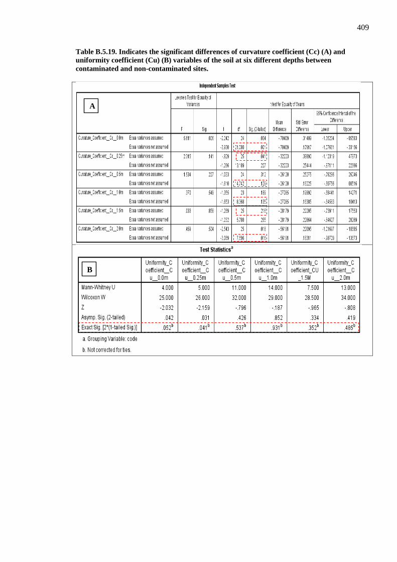
409
Table B.5.19. Indicates the significant differences of curvature coefficient (Cc) (A) and uniformity coefficient (Cu) (B) variables of the soil at six different depths between contaminated and non-contaminated sites.
A
B

410
Permeability (Hydraulic Conductivity) Table B.5.20. Coefficient of Permeability results for contaminated samples at six different
depths of 0.0 m, 0.25 m, 0.5 m, 1.0 m, 1.5 m and 2.0 m.
Trial Pits Coordinates (T.P.Cs)
Permeability coefficient Results (m/sec) Soil Classification
At Depth (0.0 m) (50 m, 0 m) 2.06x10⁻⁵ Sand (SP)
(100 m, 0 m) 1.53x10⁻⁵ Silty Sand (S-M) (50 m, 50 m) 2.33x10⁻⁵ Silty Sand (S-M) (100 m, 50 m) 4.79x10⁻⁵ Silty sand (S-M)
Min. value 1.53x10⁻⁵ - Max. value 4.79x10⁻⁵ - Mean Value 2.67x10⁻⁵ -
standard deviation value 1.44 X10⁻⁵ - At Depth (0.25 m)
(50 m, 0 m) *Nil Silty Sand (S-M) (100 m, 0 m) *Nil Silty Sand (S-M) (50 m, 50 m) 1.78x 10⁻⁵ Silty Sand (S-M) (100 m, 50 m) 6.59x 10⁻⁶ Silty Sand (S-M)
Min. value 6.59x 10⁻⁶ - Max. value 1.78x 10⁻⁵ - Mean Value 6.1x 10⁻⁶ -
standard deviation value 7.92x10⁻⁶ - At Depth (0.5 m)
(50 m, 0 m) *Nil Sand (SP) (100 m, 0 m) 1.07x10⁻⁵ Silty Sand (S-M) (50 m, 50 m) *Nil Silty Sand (S-M) (100 m, 50 m) 8.56x10⁻⁶ Sand with silt (S-M)
Min. value 8.56x10⁻⁶ - Max. value 1.07x10⁻⁵ - Mean Value 4.81 x 10⁻⁶ -
standard deviation value 1.51x 10⁻⁶ - At Depth (1.0 m)
(50 m, 0 m) 3.25x10⁻⁵ Silty Sand (S-M) (100 m, 0 m) 4.64x10⁻⁵ Silty Sand (S-M) (50 m, 50 m) 2.19x10⁻⁵ Silty Sand (S-M) (100 m, 50 m) 2.66x10⁻⁵ Silty Sand (S-M)
Min. value 2.19x10⁻⁵ - Max. value 4.64x10⁻⁵ - Mean Value 3.18x10⁻⁵ -
standard deviation value 1.06x10⁻⁵ -
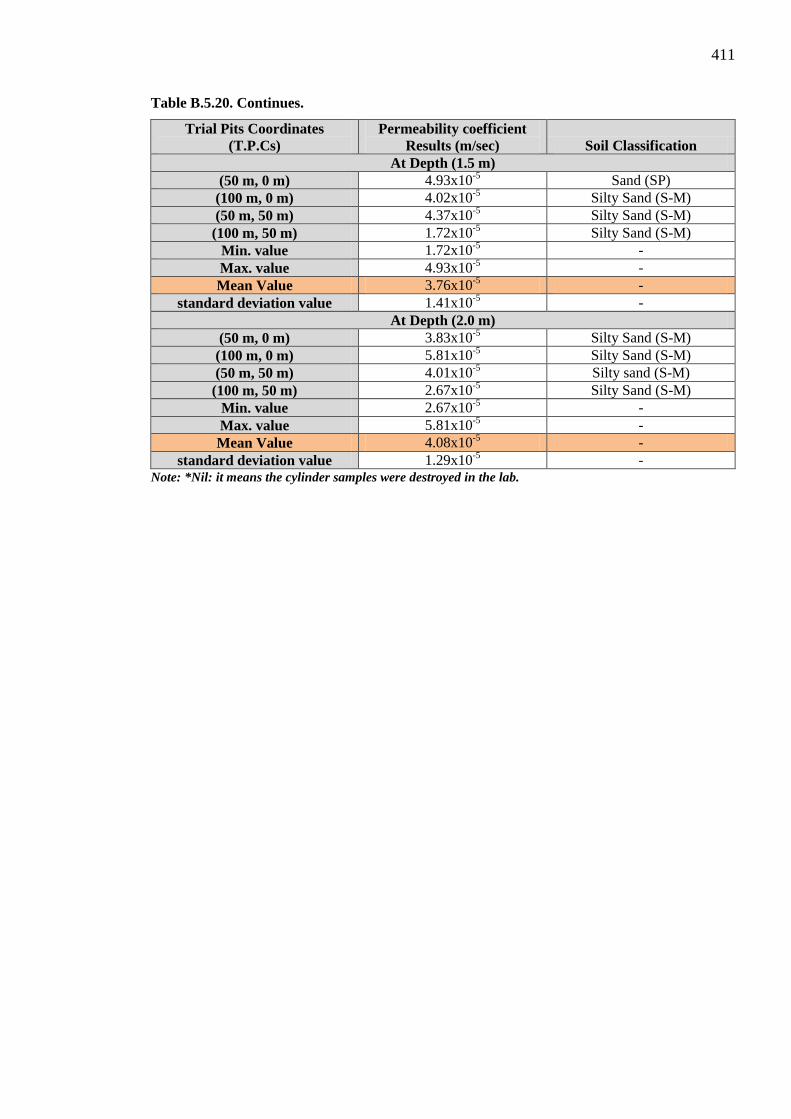
411
Table B.5.20. Continues.
Trial Pits Coordinates (T.P.Cs)
Permeability coefficient Results (m/sec) Soil Classification
At Depth (1.5 m) (50 m, 0 m) 4.93x10⁻⁵ Sand (SP) (100 m, 0 m) 4.02x10⁻⁵ Silty Sand (S-M) (50 m, 50 m) 4.37x10⁻⁵ Silty Sand (S-M)
(100 m, 50 m) 1.72x10⁻⁵ Silty Sand (S-M) Min. value 1.72x10⁻⁵ - Max. value 4.93x10⁻⁵ - Mean Value 3.76x10⁻⁵ -
standard deviation value 1.41x10⁻⁵ - At Depth (2.0 m)
(50 m, 0 m) 3.83x10⁻⁵ Silty Sand (S-M) (100 m, 0 m) 5.81x10⁻⁵ Silty Sand (S-M) (50 m, 50 m) 4.01x10⁻⁵ Silty sand (S-M)
(100 m, 50 m) 2.67x10⁻⁵ Silty Sand (S-M) Min. value 2.67x10⁻⁵ - Max. value 5.81x10⁻⁵ - Mean Value 4.08x10⁻⁵ -
standard deviation value 1.29x10⁻⁵ - Note: *Nil: it means the cylinder samples were destroyed in the lab.

412
Table B.5.21. Coefficient of permeability results for non-contaminated samples at six
different depths of 0.0 m, 0.25 m, 0.5 m and 1.0 m, 1.5 m and 2.0 m.
Trial Pits Coordinates (T.P.Cs)
Permeability Coefficient Results
(m/sec) Soil Classification At Depth (0.0 m)
(0 m, 0 m) 3.05x10⁻⁵ silty SAND (S-M). (50 m, 50 m) 1.14x10⁻⁵ silty SAND (S-M). Min. value 1.14x10⁻⁵ - Max. value 3.05x10⁻⁵ - Mean Value 2.09x10⁻⁵ -
standard deviation value 1.35x10⁻⁵ - At Depth (0.25 m)
(0 m, 0 m) 7.69x10⁻⁵ silty SAND (S-M). (50 m, 50 m) 1.34x10⁻⁴ silty SAND (S-M). Min. value 7.69x10⁻⁵ - Max. value 1.34x10⁻⁴ - Mean Value 1.05x10⁻⁴ -
standard deviation value 4.03x10⁻⁵ - At Depth (0.5 m)
(0 m, 0 m) 9.58x10⁻⁵ silty sand (S-M) (50 m, 50 m) 7.63x10⁻⁶ silty SAND (S-M). Min. value 7.63x10⁻⁶ - Max. value 9.58x10⁻⁵ - Mean Value 5.17x10⁻⁵ -
standard deviation value 6.23x10⁻⁵ - At Depth (1.0 m)
(0 m, 0 m) 4.82x10⁻⁵ Very silty SAND (SM). (50 m, 50 m) 1.03x10⁻⁶ silty SAND (S-M). Min. value 1.03x10⁻⁶ - Max. value 4.82x10⁻⁵ - Mean Value 2.46x10⁻⁵ -
standard deviation value 3.33x10⁻⁵ - At Depth (1.5 m)
(0 m, 0 m) 3.49x10⁻⁵ Silty Sand (S-M) (50 m, 50 m) 1.63x10⁻⁵ Silty Sand (S-M) Min. value 1.63x10⁻⁵ - Max. value 3.49x10⁻⁵ - Mean Value 2.56x10⁻⁵ -
standard deviation value 1.31x10⁻⁵ - At Depth (2.0 m)
(0 m, 0 m) 3.12x10⁻⁶ Silty Sand (S-M) (50 m, 50 m) 2.23x10⁻⁵ Silty Sand (S-M) Min. value 3.12x10⁻⁶ - Max. value 2.23x10⁻⁵ - Mean Value 1.27x10⁻⁵ -
standard deviation value 1.35x10⁻⁵ -
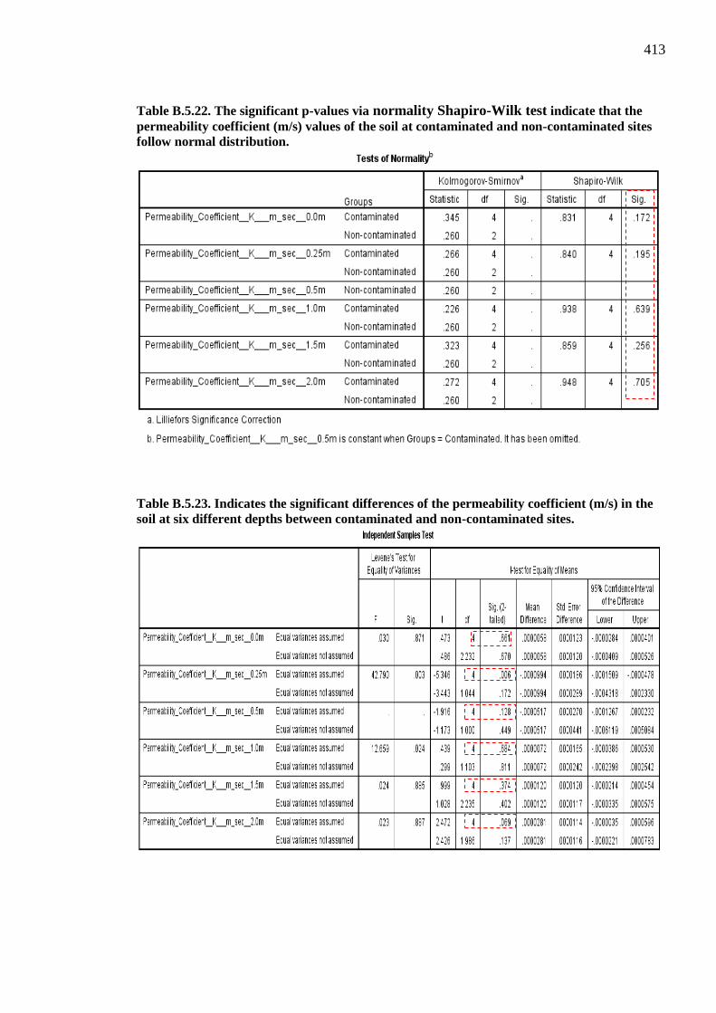
413
Table B.5.22. The significant p-values via normality Shapiro-Wilk test indicate that the permeability coefficient (m/s) values of the soil at contaminated and non-contaminated sites follow normal distribution.
Table B.5.23. Indicates the significant differences of the permeability coefficient (m/s) in the soil at six different depths between contaminated and non-contaminated sites.

414
Direct Shear test Table B.5.24. Angle of internal friction (φ) results for contaminated soil samples at six
different depths of 0.0 m, 0.25 m, 0.5 m, 1.0 m, 1.5 m and 2.0 m.
Trial Pits Coordinates (T.P.Cs)
Strength Parameters (φ) Angle of Internal Friction
(φ) At Depth (0.0 m)
(0 m, 0 m) 33 (50 m, 0 m) 32 (0 m, 50 m) 35
(50 m, 50 m) 28 (100 m, 50 m) 29 (50 m, 100 m) 29
(100 m, 100 m) 30 Min. Value 28 Max. Value 35 Mean Value 30.8
Standard deviation value 2.5 At Depth (0.25 m)
(0 m, 0 m) 34 (50 m, 0 m) 31 (0 m, 50 m) 32
(50 m, 50 m) 30 (100 m, 50 m) 34 (50 m, 100 m) 33
(100 m, 100 m) 33 Min. Value 30 Max. Value 34 Mean Value 32
Standard deviation value 1.5 At Depth (0.5 m)
(0 m, 0 m) 34 (50 m, 0 m) 33 (0 m, 50 m) 31
(50 m, 50 m) 33 (100 m, 50 m) 33 (50 m, 100 m) 34
(100 m, 100 m) 32 Min. Value 31 Max. Value 34 Mean Value 32.8
Standard deviation value 1.06 At Depth (1.0 m)
(0 m, 0 m) 34 (50 m, 0 m) 31 (0 m, 50 m) 34
(50 m, 50 m) 33 (100 m, 50 m) 33 (50 m, 100 m) 34
(100 m, 100 m) 32 Min. Value 31 Max. Value 34 Mean Value 33
Standard deviation value 1.15
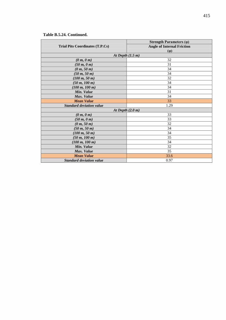
415
Table B.5.24. Continued.
Trial Pits Coordinates (T.P.Cs)
Strength Parameters (φ) Angle of Internal Friction
(φ) At Depth (1.5 m)
(0 m, 0 m) 32 (50 m, 0 m) 31 (0 m, 50 m) 34
(50 m, 50 m) 34 (100 m, 50 m) 32 (50 m, 100 m) 34
(100 m, 100 m) 34 Min. Value 31 Max. Value 34 Mean Value 33
Standard deviation value 1.29 At Depth (2.0 m)
(0 m, 0 m) 33 (50 m, 0 m) 33 (0 m, 50 m) 32
(50 m, 50 m) 34 (100 m, 50 m) 34 (50 m, 100 m) 35
(100 m, 100 m) 34 Min. Value 32 Max. Value 35 Mean Value 33.6
Standard deviation value 0.97
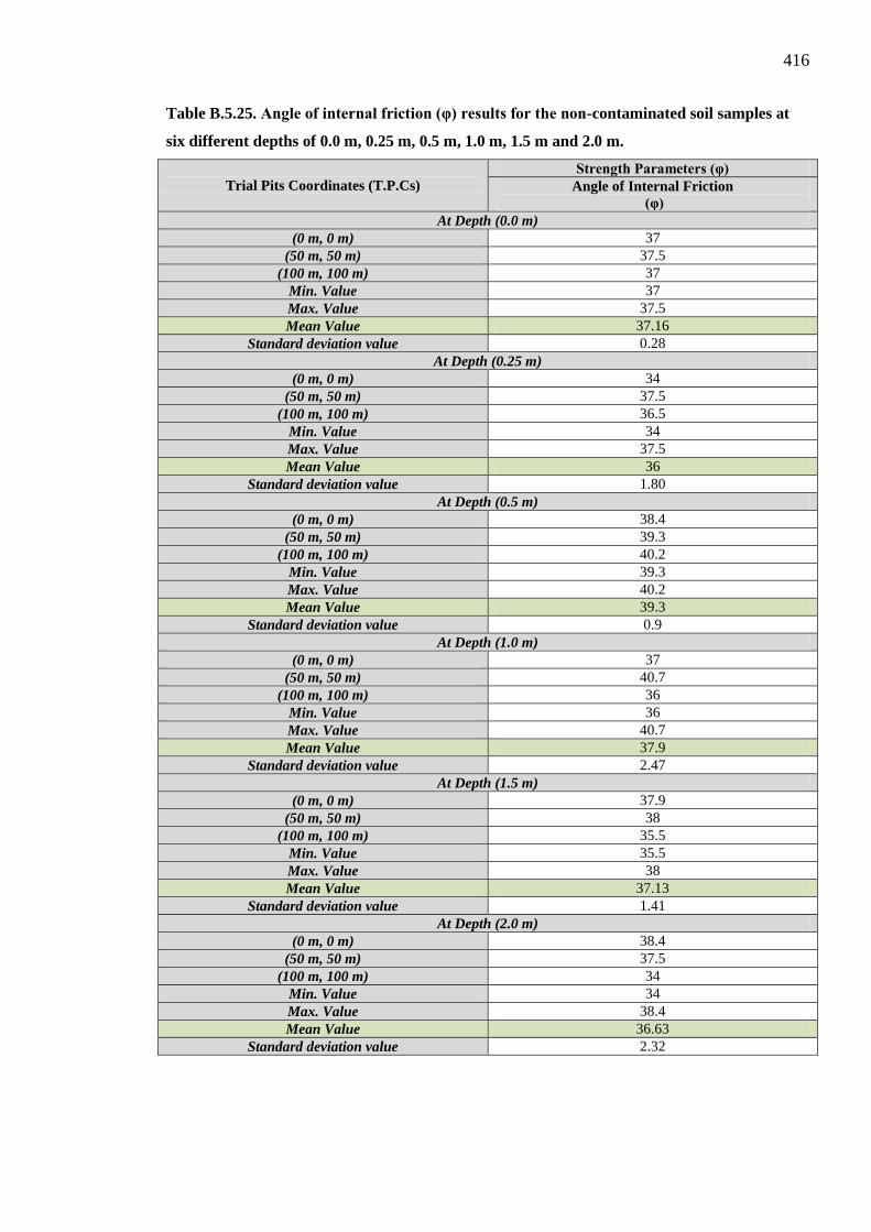
416
Table B.5.25. Angle of internal friction (φ) results for the non-contaminated soil samples at
six different depths of 0.0 m, 0.25 m, 0.5 m, 1.0 m, 1.5 m and 2.0 m.
Trial Pits Coordinates (T.P.Cs)
Strength Parameters (φ) Angle of Internal Friction
(φ) At Depth (0.0 m)
(0 m, 0 m) 37 (50 m, 50 m) 37.5
(100 m, 100 m) 37 Min. Value 37 Max. Value 37.5 Mean Value 37.16
Standard deviation value 0.28 At Depth (0.25 m)
(0 m, 0 m) 34 (50 m, 50 m) 37.5
(100 m, 100 m) 36.5 Min. Value 34 Max. Value 37.5 Mean Value 36
Standard deviation value 1.80 At Depth (0.5 m)
(0 m, 0 m) 38.4 (50 m, 50 m) 39.3
(100 m, 100 m) 40.2 Min. Value 39.3 Max. Value 40.2 Mean Value 39.3
Standard deviation value 0.9 At Depth (1.0 m)
(0 m, 0 m) 37 (50 m, 50 m) 40.7
(100 m, 100 m) 36 Min. Value 36 Max. Value 40.7 Mean Value 37.9
Standard deviation value 2.47 At Depth (1.5 m)
(0 m, 0 m) 37.9 (50 m, 50 m) 38
(100 m, 100 m) 35.5 Min. Value 35.5 Max. Value 38 Mean Value 37.13
Standard deviation value 1.41 At Depth (2.0 m)
(0 m, 0 m) 38.4 (50 m, 50 m) 37.5
(100 m, 100 m) 34 Min. Value 34 Max. Value 38.4 Mean Value 36.63
Standard deviation value 2.32
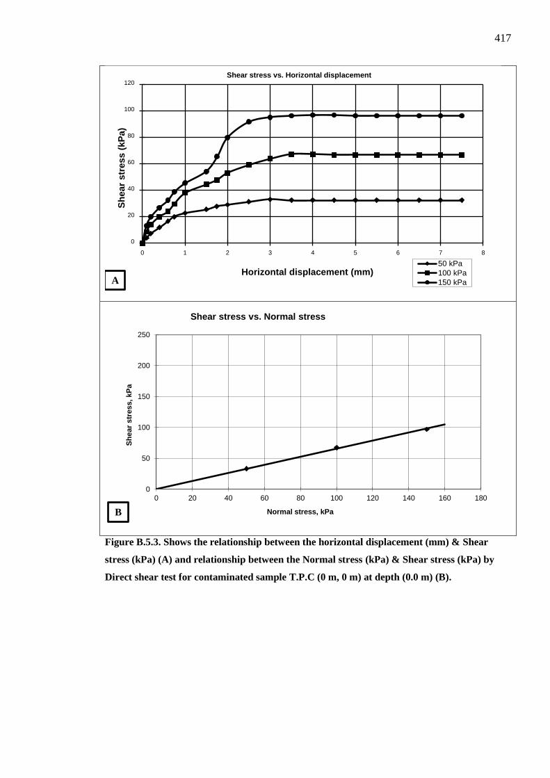
417
Figure B.5.3. Shows the relationship between the horizontal displacement (mm) & Shear
stress (kPa) (A) and relationship between the Normal stress (kPa) & Shear stress (kPa) by
Direct shear test for contaminated sample T.P.C (0 m, 0 m) at depth (0.0 m) (B).
0
20
40
60
80
100
120
0 1 2 3 4 5 6 7 8
Sh
ear
stre
ss (
kPa)
Horizontal displacement (mm)
Shear stress vs. Horizontal displacement
50 kPa100 kPa150 kPaA
0
50
100
150
200
250
0 20 40 60 80 100 120 140 160 180
Sh
ear
stre
ss, k
Pa
Normal stress, kPa
Shear stress vs. Normal stress
B

418
Figure B.5.4. Shows the relationship between the horizontal displacement (mm) & Shear
stress (kPa) (A) and relationship between the Normal stress (kPa) & Shear stress (kPa) by
Direct Shear test for contaminated sample T.P.Cs (0 m, 0 m) at depth (0.25 m) (B).
0
20
40
60
80
100
120
0 1 2 3 4 5 6 7 8
Sh
ear
stre
ss (
kPa)
Horizontal displacement (mm)
Shear stress vs. Horizontal displacement
50 kPa100 kPa150 kPa
A
0
50
100
150
200
250
0 20 40 60 80 100 120 140 160 180
Sh
ear
stre
ss, k
Pa
Normal stress, kPa
Shear stress vs. Normal stress
B

419
Figure B.5.5. Shows the relationship between the horizontal displacement (mm) & Shear
stress (kPa) (A) and relationship between the Normal stress (kPa) & Shear stress (kPa) by
Direct Shear test for contaminated sample T.P.Cs (0 m, 0 m) at depth (0.5 m) (B).
0
20
40
60
80
100
120
0 1 2 3 4 5 6 7 8
Sh
ear
stre
ss (
kPa)
Horizontal displacement (mm)
Shear stress vs. Horizontal displacement
50 kPa100 kPa150 kPaA
0
50
100
150
200
250
0 20 40 60 80 100 120 140 160 180
Sh
ear
stre
ss, k
Pa
Normal stress, kPa
Shear stress vs. Normal stress
B
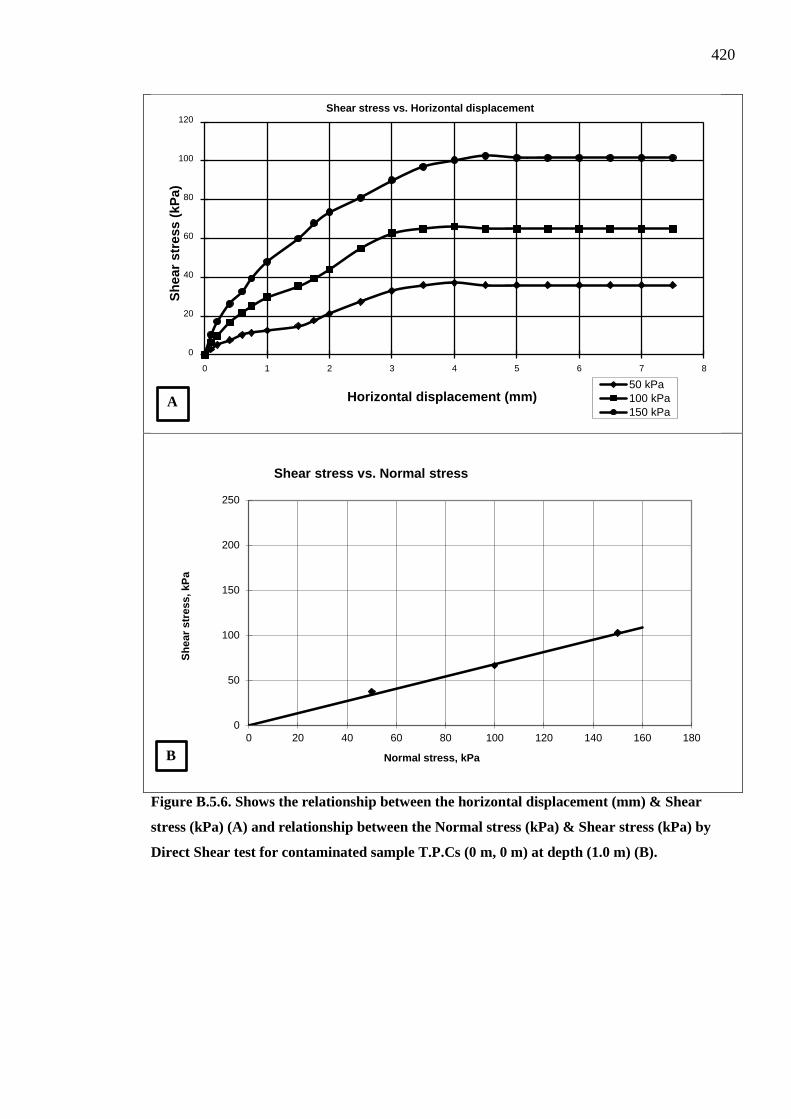
420
Figure B.5.6. Shows the relationship between the horizontal displacement (mm) & Shear
stress (kPa) (A) and relationship between the Normal stress (kPa) & Shear stress (kPa) by
Direct Shear test for contaminated sample T.P.Cs (0 m, 0 m) at depth (1.0 m) (B).
0
20
40
60
80
100
120
0 1 2 3 4 5 6 7 8
Sh
ear
stre
ss (
kPa)
Horizontal displacement (mm)
Shear stress vs. Horizontal displacement
50 kPa100 kPa150 kPa
A
0
50
100
150
200
250
0 20 40 60 80 100 120 140 160 180
Sh
ear
stre
ss, k
Pa
Normal stress, kPa
Shear stress vs. Normal stress
B

421
Figure B.5.7. Shows the relationship between the horizontal displacement (mm) & Shear
stress (kPa) (A) and relationship between the Normal stress (kPa) & Shear stress (kPa) by
Direct Shear test for contaminated sample T.P.Cs (0 m, 0 m) at depth (1.5 m) (B).
0
10
20
30
40
50
60
70
80
90
100
0 1 2 3 4 5 6 7 8
Sh
ear
stre
ss (
kPa)
Horizontal displacement (mm)
Shear stress vs. Horizontal displacement
50 kPa100 kPa150 kPaA
0
50
100
150
200
250
0 20 40 60 80 100 120 140 160 180
Sh
ear
stre
ss, k
Pa
Normal stress, kPa
Shear stress vs. Normal stress
B
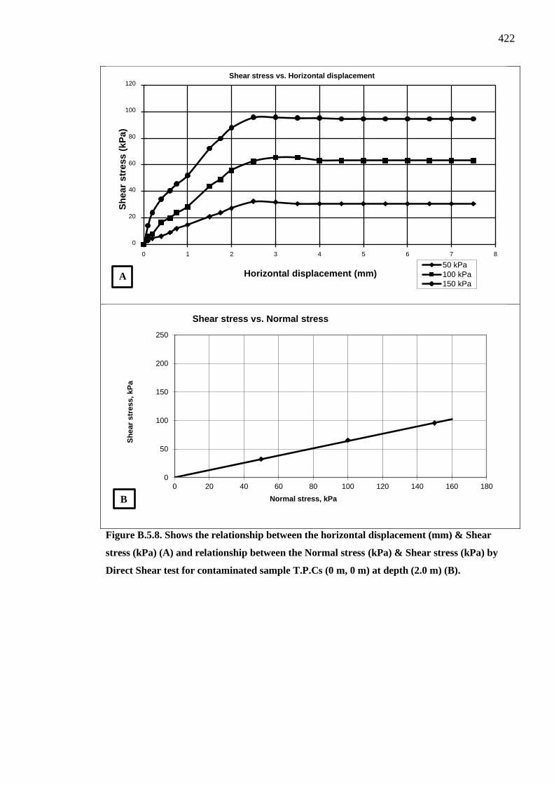
422
Figure B.5.8. Shows the relationship between the horizontal displacement (mm) & Shear
stress (kPa) (A) and relationship between the Normal stress (kPa) & Shear stress (kPa) by
Direct Shear test for contaminated sample T.P.Cs (0 m, 0 m) at depth (2.0 m) (B).
0
20
40
60
80
100
120
0 1 2 3 4 5 6 7 8
Sh
ear
stre
ss (
kPa)
Horizontal displacement (mm)
Shear stress vs. Horizontal displacement
50 kPa100 kPa150 kPa
A
0
50
100
150
200
250
0 20 40 60 80 100 120 140 160 180
Sh
ear
stre
ss, k
Pa
Normal stress, kPa
Shear stress vs. Normal stress
B
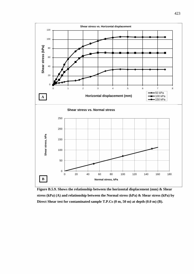
423
Figure B.5.9. Shows the relationship between the horizontal displacement (mm) & Shear
stress (kPa) (A) and relationship between the Normal stress (kPa) & Shear stress (kPa) by
Direct Shear test for contaminated sample T.P.Cs (0 m, 50 m) at depth (0.0 m) (B).
0
20
40
60
80
100
120
0 1 2 3 4 5 6 7 8
Sh
ear
stre
ss (
kPa)
Horizontal displacement (mm)
Shear stress vs. Horizontal displacement
50 kPa100 kPa150 kPa
A
0
50
100
150
200
250
0 20 40 60 80 100 120 140 160 180
Sh
ear
stre
ss, k
Pa
Normal stress, kPa
Shear stress vs. Normal stress
B
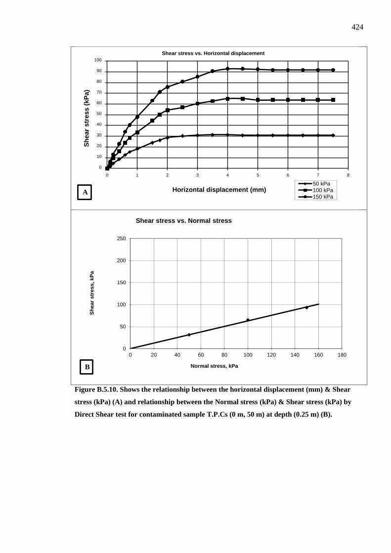
424
Figure B.5.10. Shows the relationship between the horizontal displacement (mm) & Shear
stress (kPa) (A) and relationship between the Normal stress (kPa) & Shear stress (kPa) by
Direct Shear test for contaminated sample T.P.Cs (0 m, 50 m) at depth (0.25 m) (B).
0
10
20
30
40
50
60
70
80
90
100
0 1 2 3 4 5 6 7 8
Sh
ear
stre
ss (
kPa)
Horizontal displacement (mm)
Shear stress vs. Horizontal displacement
50 kPa100 kPa150 kPa
A
0
50
100
150
200
250
0 20 40 60 80 100 120 140 160 180
Sh
ear
stre
ss, k
Pa
Normal stress, kPa
Shear stress vs. Normal stress
B

425
Figure B.5.11. Shows the relationship between the horizontal displacement (mm) & Shear
stress (kPa) (A) and relationship between the Normal stress (kPa) & Shear stress (kPa) by
Direct Shear test for contaminated sample T.P.Cs (0 m, 50 m) at depth (0.5 m) (B).
0
10
20
30
40
50
60
70
80
90
100
0 1 2 3 4 5 6 7 8
Sh
ear
stre
ss (
kPa)
Horizontal displacement (mm)
Shear stress vs. Horizontal displacement
50 kPa100 kPa150 kPa
A
0
50
100
150
200
250
0 20 40 60 80 100 120 140 160 180
Sh
ear
stre
ss, k
Pa
Normal stress, kPa
Shear stress vs. Normal stress
B
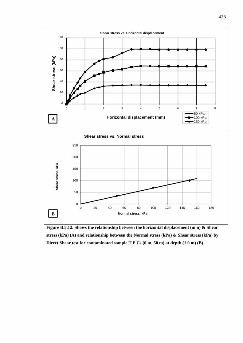
426
Figure B.5.12. Shows the relationship between the horizontal displacement (mm) & Shear
stress (kPa) (A) and relationship between the Normal stress (kPa) & Shear stress (kPa) by
Direct Shear test for contaminated sample T.P.Cs (0 m, 50 m) at depth (1.0 m) (B).
0
20
40
60
80
100
120
0 1 2 3 4 5 6 7 8
Sh
ear
stre
ss (
kPa)
Horizontal displacement (mm)
Shear stress vs. Horizontal displacement
50 kPa100 kPa150 kPa
A
0
50
100
150
200
250
0 20 40 60 80 100 120 140 160 180
Sh
ear
stre
ss, k
Pa
Normal stress, kPa
Shear stress vs. Normal stress
B
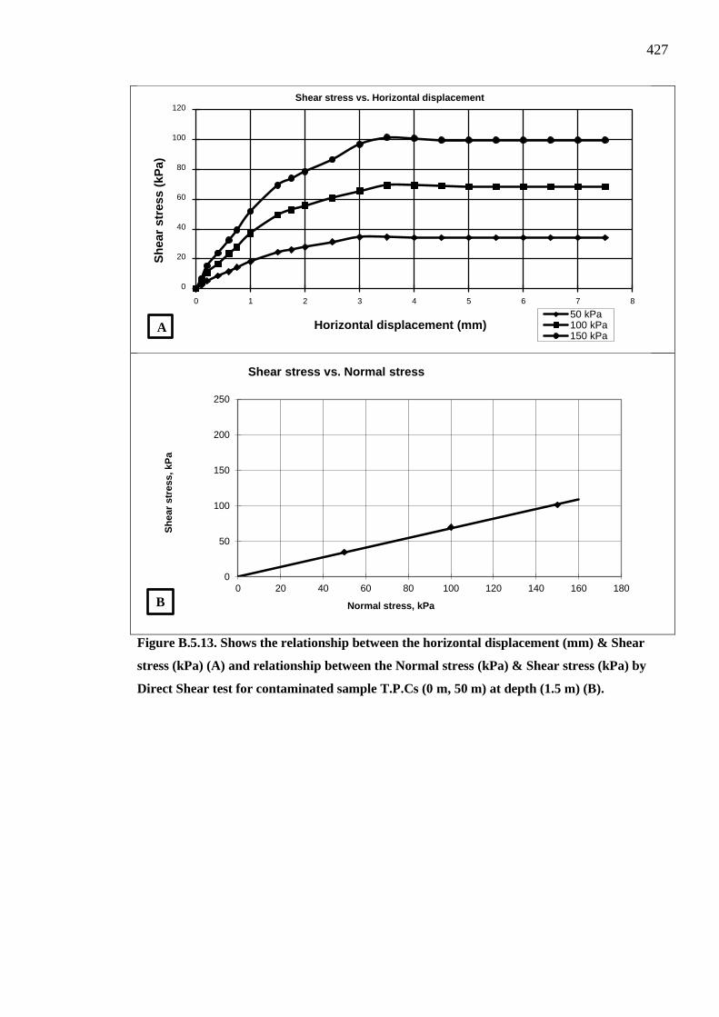
427
Figure B.5.13. Shows the relationship between the horizontal displacement (mm) & Shear
stress (kPa) (A) and relationship between the Normal stress (kPa) & Shear stress (kPa) by
Direct Shear test for contaminated sample T.P.Cs (0 m, 50 m) at depth (1.5 m) (B).
0
20
40
60
80
100
120
0 1 2 3 4 5 6 7 8
Sh
ear
stre
ss (
kPa)
Horizontal displacement (mm)
Shear stress vs. Horizontal displacement
50 kPa100 kPa150 kPa
A
0
50
100
150
200
250
0 20 40 60 80 100 120 140 160 180
Sh
ear
stre
ss, k
Pa
Normal stress, kPa
Shear stress vs. Normal stress
B

428
Figure B.5.14. Shows the relationship between the horizontal displacement (mm) & Shear
stress (kPa) (A) and relationship between the Normal stress (kPa) & Shear stress (kPa) by
Direct Shear test for contaminated sample T.P.Cs (0 m, 50 m) at depth (2.0 m) (B).
0
20
40
60
80
100
120
0 1 2 3 4 5 6 7 8
Sh
ear
stre
ss (
kPa)
Horizontal displacement (mm)
Shear stress vs. Horizontal displacement
50 kPa100 kPa150 kPaA
0
50
100
150
200
250
0 20 40 60 80 100 120 140 160 180
Sh
ear
stre
ss, k
Pa
Normal stress, kPa
Shear stress vs. Normal stress
B

429
Figure B.5.15. Shows the relationship between the horizontal displacement (mm) & Shear
stress (kPa) (A) and relationship between the Normal stress (kPa) & Shear stress (kPa) by
Direct Shear test for contaminated sample T.P.Cs (50 m, 50 m) at depth (0.0 m) (B).
0
10
20
30
40
50
60
70
80
90
100
0 1 2 3 4 5 6 7 8
Sh
ear
stre
ss (
kPa)
Horizontal displacement (mm)
Shear stress vs. Horizontal displacement
50 kPa100 kPa150 kPa
A
0
50
100
150
200
250
0 20 40 60 80 100 120 140 160 180
Sh
ear
stre
ss, k
Pa
Normal stress, kPa
Shear stress vs. Normal stress
B
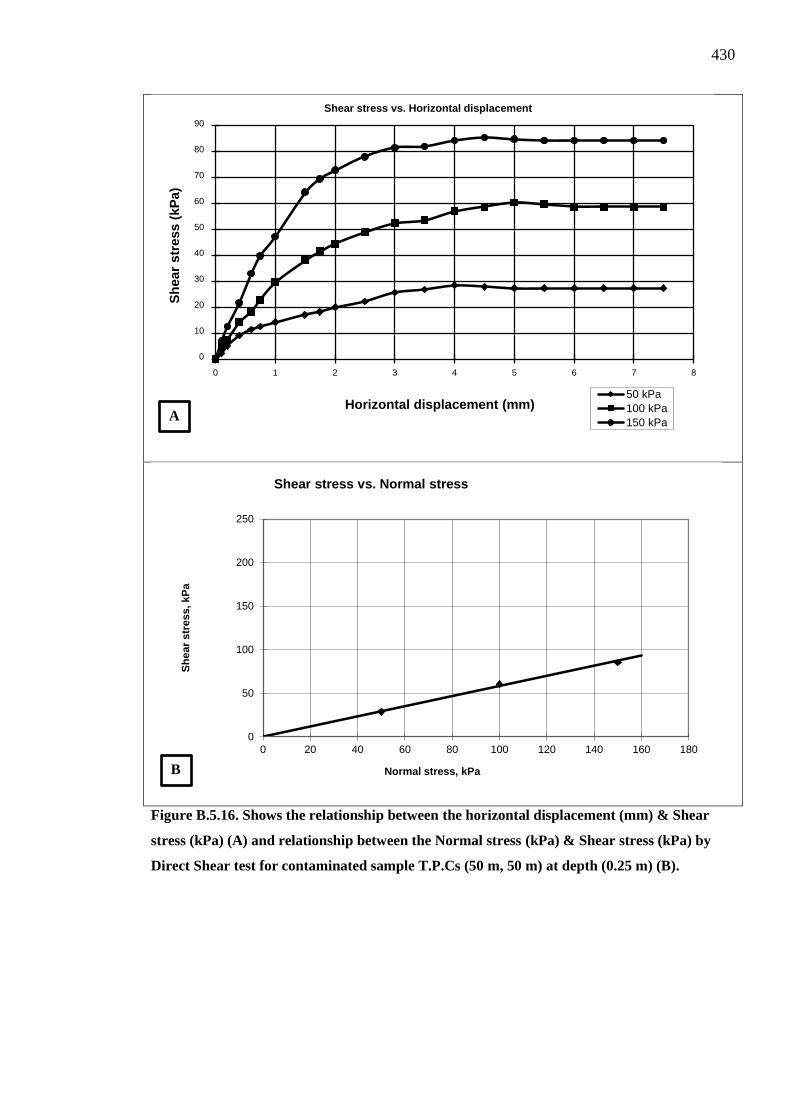
430
Figure B.5.16. Shows the relationship between the horizontal displacement (mm) & Shear
stress (kPa) (A) and relationship between the Normal stress (kPa) & Shear stress (kPa) by
Direct Shear test for contaminated sample T.P.Cs (50 m, 50 m) at depth (0.25 m) (B).
0
10
20
30
40
50
60
70
80
90
0 1 2 3 4 5 6 7 8
Sh
ear
stre
ss (
kPa)
Horizontal displacement (mm)
Shear stress vs. Horizontal displacement
50 kPa100 kPa150 kPaA
0
50
100
150
200
250
0 20 40 60 80 100 120 140 160 180
Sh
ear
stre
ss, k
Pa
Normal stress, kPa
Shear stress vs. Normal stress
B
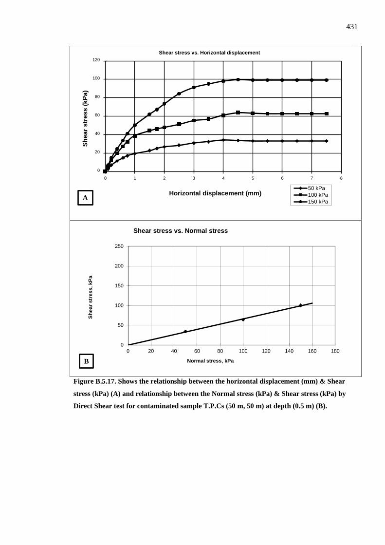
431
Figure B.5.17. Shows the relationship between the horizontal displacement (mm) & Shear
stress (kPa) (A) and relationship between the Normal stress (kPa) & Shear stress (kPa) by
Direct Shear test for contaminated sample T.P.Cs (50 m, 50 m) at depth (0.5 m) (B).
0
20
40
60
80
100
120
0 1 2 3 4 5 6 7 8
Sh
ear
stre
ss (
kPa)
Horizontal displacement (mm)
Shear stress vs. Horizontal displacement
50 kPa100 kPa150 kPa
A
0
50
100
150
200
250
0 20 40 60 80 100 120 140 160 180
Sh
ear
stre
ss, k
Pa
Normal stress, kPa
Shear stress vs. Normal stress
B

432
Figure B.5.18. Shows the relationship between the horizontal displacement (mm) & Shear
stress (kPa) (A) and relationship between the Normal stress (kPa) & Shear stress (kPa) by
Direct Shear test for contaminated sample T.P.Cs (50 m, 50 m) at depth (1.0 m) (B).
0
10
20
30
40
50
60
70
80
90
100
0 1 2 3 4 5 6 7 8
Sh
ear
stre
ss (
kPa)
Horizontal displacement (mm)
Shear stress vs. Horizontal displacement
50 kPa100 kPa150 kPa
A
0
50
100
150
200
250
0 20 40 60 80 100 120 140 160 180
Sh
ear
stre
ss, k
Pa
Normal stress, kPa
Shear stress vs. Normal stress
B

433
Figure B.5.19. Shows the relationship between the horizontal displacement (mm) & Shear
stress (kPa) (A) and relationship between the Normal stress (kPa) & Shear stress (kPa) by
Direct Shear test for contaminated sample T.P.Cs (50 m, 50 m) at depth (1.5 m) (B).
0
20
40
60
80
100
120
0 1 2 3 4 5 6 7 8
Sh
ear
stre
ss (
kPa)
Horizontal displacement (mm)
Shear stress vs. Horizontal displacement
50 kPa100 kPa150 kPa
A
0
50
100
150
200
250
0 20 40 60 80 100 120 140 160 180
Sh
ear
stre
ss, k
Pa
Normal stress, kPa
Shear stress vs. Normal stress
B

434
Figure B.5.20. Shows the relationship between the horizontal displacement (mm) & Shear
stress (kPa) (A) and relationship between the Normal stress (kPa) & Shear stress (kPa) by
Direct Shear test for contaminated sample T.P.Cs (50 m, 50 m) at depth (2.0 m) (B).
0
20
40
60
80
100
120
0 1 2 3 4 5 6 7 8
Sh
ear
stre
ss (
kPa)
Horizontal displacement (mm)
Shear stress vs. Horizontal displacement
50 kPa100 kPa150 kPaA
0
50
100
150
200
250
0 20 40 60 80 100 120 140 160 180
Sh
ear
stre
ss, k
Pa
Normal stress, kPa
Shear stress vs. Normal stress
B

435
Figure B.5.21. Shows the relationship between the horizontal displacement (mm) & Shear
stress (kPa) (A) and relationship between the Normal stress (kPa) & Shear stress (kPa) by
Direct Shear test for contaminated sample T.P.Cs (50 m, 0 m) at depth (0.0 m) (B).
0
10
20
30
40
50
60
70
80
90
100
0 1 2 3 4 5 6 7 8
Sh
ear
stre
ss (
kPa)
Horizontal displacement (mm)
Shear stress vs. Horizontal displacement
50 kPa100 kPa150 kPa
A
0
50
100
150
200
250
0 20 40 60 80 100 120 140 160 180
Sh
ear
stre
ss, k
Pa
Normal stress, kPa
Shear stress vs. Normal stress
B
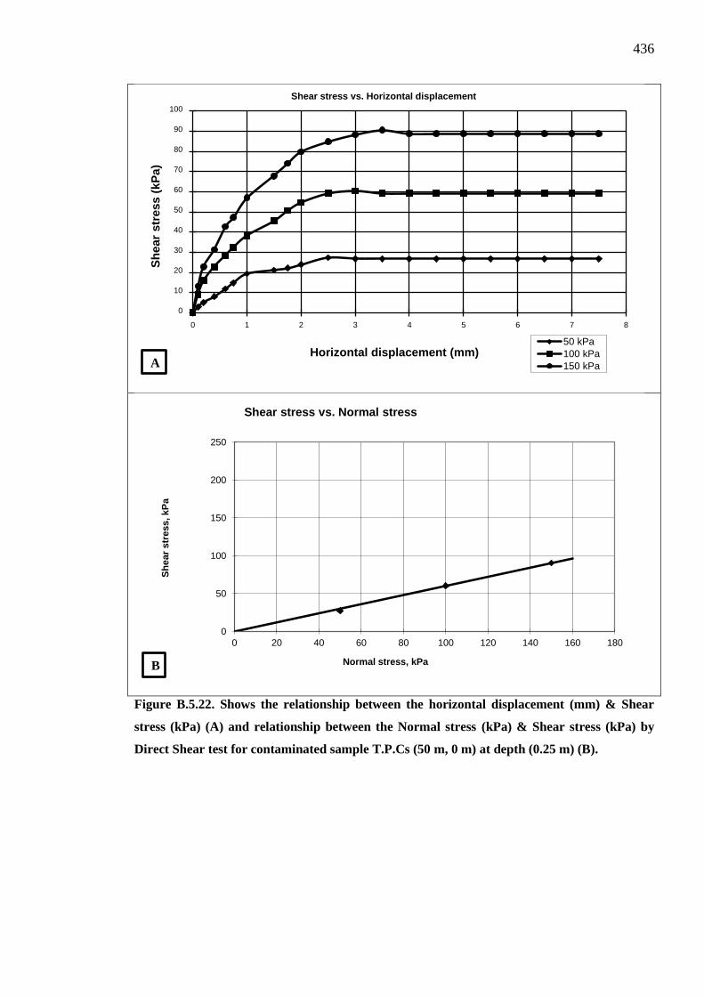
436
Figure B.5.22. Shows the relationship between the horizontal displacement (mm) & Shear
stress (kPa) (A) and relationship between the Normal stress (kPa) & Shear stress (kPa) by
Direct Shear test for contaminated sample T.P.Cs (50 m, 0 m) at depth (0.25 m) (B).
0
10
20
30
40
50
60
70
80
90
100
0 1 2 3 4 5 6 7 8
Sh
ear
stre
ss (
kPa)
Horizontal displacement (mm)
Shear stress vs. Horizontal displacement
50 kPa100 kPa150 kPaA
0
50
100
150
200
250
0 20 40 60 80 100 120 140 160 180
Sh
ear
stre
ss, k
Pa
Normal stress, kPa
Shear stress vs. Normal stress
B
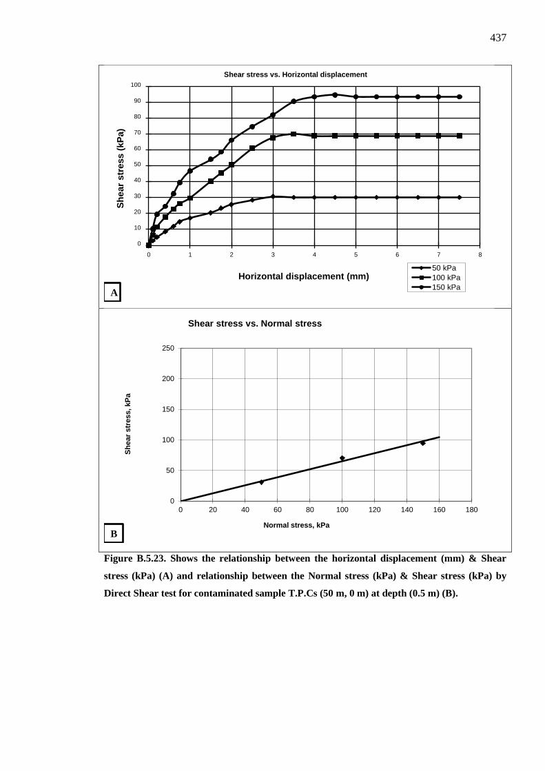
437
Figure B.5.23. Shows the relationship between the horizontal displacement (mm) & Shear
stress (kPa) (A) and relationship between the Normal stress (kPa) & Shear stress (kPa) by
Direct Shear test for contaminated sample T.P.Cs (50 m, 0 m) at depth (0.5 m) (B).
0
10
20
30
40
50
60
70
80
90
100
0 1 2 3 4 5 6 7 8
Sh
ear
stre
ss (
kPa)
Horizontal displacement (mm)
Shear stress vs. Horizontal displacement
50 kPa100 kPa150 kPa
A
0
50
100
150
200
250
0 20 40 60 80 100 120 140 160 180
Sh
ear
stre
ss, k
Pa
Normal stress, kPa
Shear stress vs. Normal stress
B

438
Figure B.5.24. Shows the relationship between the horizontal displacement (mm) & Shear
stress (kPa) (A) and relationship between the Normal stress (kPa) & Shear stress (kPa) by
Direct Shear test for contaminated sample T.P.Cs (50 m, 0 m) at depth (1.0 m) (B).
0
10
20
30
40
50
60
70
80
90
100
0 1 2 3 4 5 6 7 8
Sh
ear
stre
ss (
kPa)
Horizontal displacement (mm)
Shear stress vs. Horizontal displacement
50 kPa100 kPa150 kPa
A
0
50
100
150
200
250
0 20 40 60 80 100 120 140 160 180
Sh
ear
stre
ss, k
Pa
Normal stress, kPa
Shear stress vs. Normal stress
B
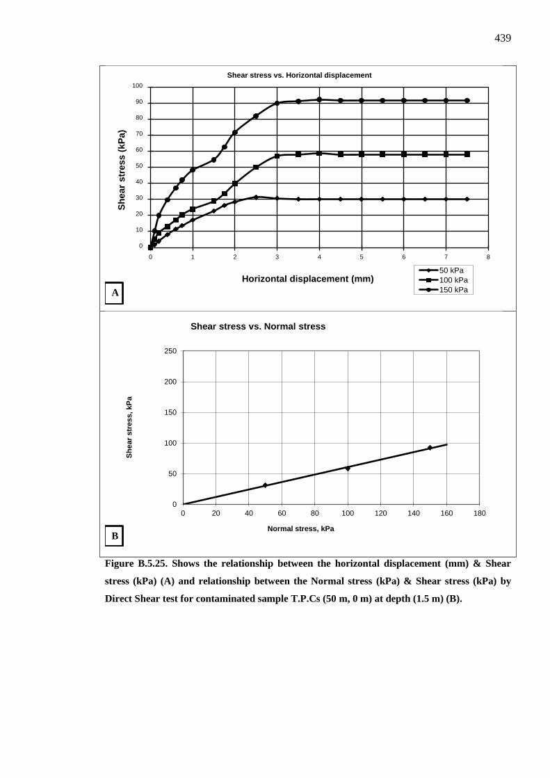
439
Figure B.5.25. Shows the relationship between the horizontal displacement (mm) & Shear
stress (kPa) (A) and relationship between the Normal stress (kPa) & Shear stress (kPa) by
Direct Shear test for contaminated sample T.P.Cs (50 m, 0 m) at depth (1.5 m) (B).
0
10
20
30
40
50
60
70
80
90
100
0 1 2 3 4 5 6 7 8
Sh
ear
stre
ss (
kPa)
Horizontal displacement (mm)
Shear stress vs. Horizontal displacement
50 kPa100 kPa150 kPaA
0
50
100
150
200
250
0 20 40 60 80 100 120 140 160 180
Sh
ear
stre
ss, k
Pa
Normal stress, kPa
Shear stress vs. Normal stress
B

440
Figure B.5.26. Shows the relationship between the horizontal displacement (mm) & Shear
stress (kPa) (A) and relationship between the Normal stress (kPa) & Shear stress (kPa) by
Direct Shear test for contaminated sample T.P.Cs (50 m, 0 m) at depth (2.0 m) (B).
0
20
40
60
80
100
120
0 1 2 3 4 5 6 7 8
Sh
ear
stre
ss (
kPa)
Horizontal displacement (mm)
Shear stress vs. Horizontal displacement
50 kPa100 kPa150 kPaA
0
50
100
150
200
250
0 20 40 60 80 100 120 140 160 180
Sh
ear
stre
ss, k
Pa
Normal stress, kPa
Shear stress vs. Normal stress
B
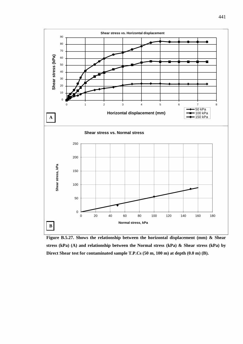
441
Figure B.5.27. Shows the relationship between the horizontal displacement (mm) & Shear
stress (kPa) (A) and relationship between the Normal stress (kPa) & Shear stress (kPa) by
Direct Shear test for contaminated sample T.P.Cs (50 m, 100 m) at depth (0.0 m) (B).
0
10
20
30
40
50
60
70
80
90
0 1 2 3 4 5 6 7 8
Sh
ear
stre
ss (
kPa)
Horizontal displacement (mm)
Shear stress vs. Horizontal displacement
50 kPa100 kPa150 kPaA
0
50
100
150
200
250
0 20 40 60 80 100 120 140 160 180
Sh
ear
stre
ss, k
Pa
Normal stress, kPa
Shear stress vs. Normal stress
B

442
Figure B.5.28. Shows the relationship between the horizontal displacement (mm) & Shear
stress (kPa) (A) and relationship between the Normal stress (kPa) & Shear stress (kPa) by
Direct Shear test for contaminated sample T.P.Cs (50 m, 100 m) at depth (0.25 m) (B).
0
20
40
60
80
100
120
0 1 2 3 4 5 6 7 8
Sh
ear
stre
ss (
kPa)
Horizontal displacement (mm)
Shear stress vs. Horizontal displacement
50 kPa100 kPa150 kPaA
0
50
100
150
200
250
0 20 40 60 80 100 120 140 160 180
Sh
ear
stre
ss, k
Pa
Normal stress, kPa
Shear stress vs. Normal stress
B

443
Figure B.5.29. Shows the relationship between the horizontal displacement (mm) & Shear
stress (kPa) (A) and relationship between the Normal stress (kPa) & Shear stress (kPa) by
Direct Shear test for contaminated sample T.P.Cs (50 m, 100 m) at depth (0.5 m) (B).
0
20
40
60
80
100
120
0 1 2 3 4 5 6 7 8
Sh
ear
stre
ss (
kPa)
Horizontal displacement (mm)
Shear stress vs. Horizontal displacement
50 kPa100 kPa150 kPaA
0
50
100
150
200
250
0 20 40 60 80 100 120 140 160 180
Sh
ear
stre
ss, k
Pa
Normal stress, kPa
Shear stress vs. Normal stress
B

444
Figure B.5.30. Shows the relationship between the horizontal displacement (mm) & Shear
stress (kPa) (A) and relationship between the Normal stress (kPa) & Shear stress (kPa) by
Direct Shear test for contaminated sample T.P.Cs (50 m, 100 m) at depth (1.0 m) (B).
0
20
40
60
80
100
120
0 1 2 3 4 5 6 7 8
Sh
ear
stre
ss (
kPa)
Horizontal displacement (mm)
Shear stress vs. Horizontal displacement
50 kPa100 kPa150 kPaA
0
50
100
150
200
250
0 20 40 60 80 100 120 140 160 180
Sh
ear
stre
ss, k
Pa
Normal stress, kPa
Shear stress vs. Normal stress
B
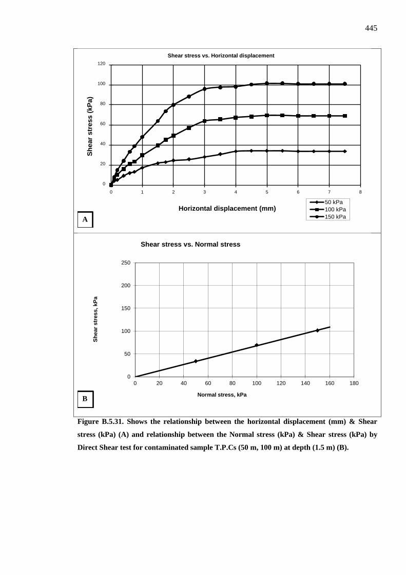
445
Figure B.5.31. Shows the relationship between the horizontal displacement (mm) & Shear
stress (kPa) (A) and relationship between the Normal stress (kPa) & Shear stress (kPa) by
Direct Shear test for contaminated sample T.P.Cs (50 m, 100 m) at depth (1.5 m) (B).
0
20
40
60
80
100
120
0 1 2 3 4 5 6 7 8
Sh
ear
stre
ss (
kPa)
Horizontal displacement (mm)
Shear stress vs. Horizontal displacement
50 kPa100 kPa150 kPaA
0
50
100
150
200
250
0 20 40 60 80 100 120 140 160 180
Sh
ear
stre
ss, k
Pa
Normal stress, kPa
Shear stress vs. Normal stress
B
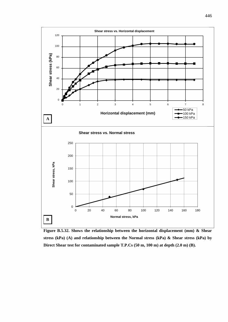
446
Figure B.5.32. Shows the relationship between the horizontal displacement (mm) & Shear
stress (kPa) (A) and relationship between the Normal stress (kPa) & Shear stress (kPa) by
Direct Shear test for contaminated sample T.P.Cs (50 m, 100 m) at depth (2.0 m) (B).
0
20
40
60
80
100
120
0 1 2 3 4 5 6 7 8
Sh
ear
stre
ss (
kPa)
Horizontal displacement (mm)
Shear stress vs. Horizontal displacement
50 kPa100 kPa150 kPaA
0
50
100
150
200
250
0 20 40 60 80 100 120 140 160 180
Sh
ear
stre
ss, k
Pa
Normal stress, kPa
Shear stress vs. Normal stress
B
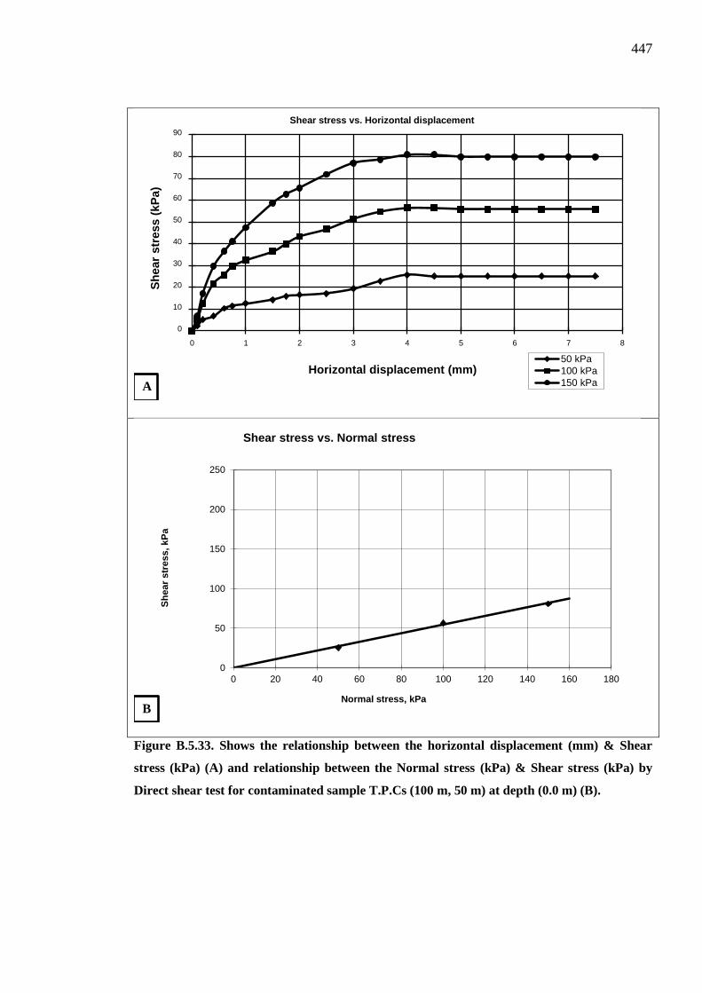
447
Figure B.5.33. Shows the relationship between the horizontal displacement (mm) & Shear
stress (kPa) (A) and relationship between the Normal stress (kPa) & Shear stress (kPa) by
Direct shear test for contaminated sample T.P.Cs (100 m, 50 m) at depth (0.0 m) (B).
0
10
20
30
40
50
60
70
80
90
0 1 2 3 4 5 6 7 8
Sh
ear
stre
ss (
kPa)
Horizontal displacement (mm)
Shear stress vs. Horizontal displacement
50 kPa100 kPa150 kPaA
0
50
100
150
200
250
0 20 40 60 80 100 120 140 160 180
Sh
ear
stre
ss, k
Pa
Normal stress, kPa
Shear stress vs. Normal stress
B

448
Figure B.5.34. Shows the relationship between the horizontal displacement (mm) & Shear
stress (kPa) (A) and relationship between the Normal stress (kPa) & Shear stress (kPa) by
Direct Shear test for contaminated sample T.P.Cs (100 m, 50 m) at depth (0.25 m) (B).
0
20
40
60
80
100
120
0 1 2 3 4 5 6 7 8
Sh
ear
stre
ss (
kPa)
Horizontal displacement (mm)
Shear stress vs. Horizontal displacement
50 kPa100 kPa150 kPaA
0
50
100
150
200
250
0 20 40 60 80 100 120 140 160 180
Sh
ear
stre
ss, k
Pa
Normal stress, kPa
Shear stress vs. Normal stress
B

449
Figure B.5.35. Shows the relationship between the horizontal displacement (mm) & Shear
stress (kPa) (A) and relationship between the Normal stress (kPa) & Shear stress (kPa) by
Direct Shear test for contaminated sample T.P.Cs (100 m, 50 m) at depth (0.5 m) (B).
0
10
20
30
40
50
60
70
80
90
100
0 1 2 3 4 5 6 7 8
Sh
ear
stre
ss (
kPa)
Horizontal displacement (mm)
Shear stress vs. Horizontal displacement
50 kPa100 kPa150 kPaA
0
50
100
150
200
250
0 20 40 60 80 100 120 140 160 180
Sh
ear
stre
ss, k
Pa
Normal stress, kPa
Shear stress vs. Normal stress
B

450
Figure B.5.36. Shows the relationship between the horizontal displacement (mm) & Shear
stress (kPa) (A) and relationship between the Normal stress (kPa) & Shear stress (kPa) by
Direct Shear test for contaminated sample T.P.Cs (100 m, 50 m) at depth (1.0 m) (B).
0
10
20
30
40
50
60
70
80
90
100
0 1 2 3 4 5 6 7 8
Sh
ear
stre
ss (
kPa)
Horizontal displacement (mm)
Shear stress vs. Horizontal displacement
50 kPa100 kPa150 kPaA
0
50
100
150
200
250
0 20 40 60 80 100 120 140 160 180
Sh
ear
stre
ss, k
Pa
Normal stress, kPa
Shear stress vs. Normal stress
B
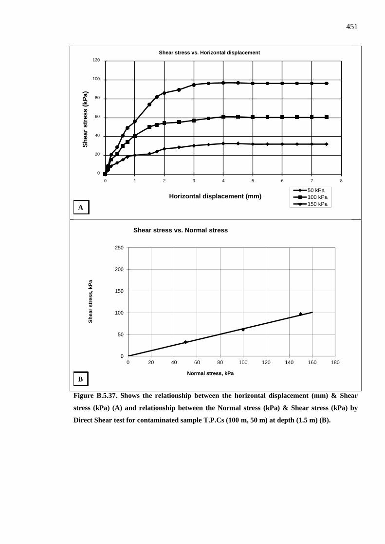
451
Figure B.5.37. Shows the relationship between the horizontal displacement (mm) & Shear
stress (kPa) (A) and relationship between the Normal stress (kPa) & Shear stress (kPa) by
Direct Shear test for contaminated sample T.P.Cs (100 m, 50 m) at depth (1.5 m) (B).
0
20
40
60
80
100
120
0 1 2 3 4 5 6 7 8
Sh
ear
stre
ss (
kPa)
Horizontal displacement (mm)
Shear stress vs. Horizontal displacement
50 kPa100 kPa150 kPaA
0
50
100
150
200
250
0 20 40 60 80 100 120 140 160 180
Sh
ear
stre
ss, k
Pa
Normal stress, kPa
Shear stress vs. Normal stress
B
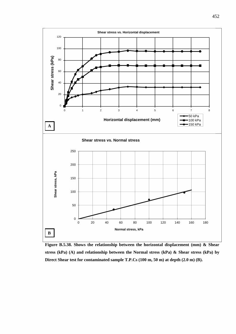
452
Figure B.5.38. Shows the relationship between the horizontal displacement (mm) & Shear
stress (kPa) (A) and relationship between the Normal stress (kPa) & Shear stress (kPa) by
Direct Shear test for contaminated sample T.P.Cs (100 m, 50 m) at depth (2.0 m) (B).
0
20
40
60
80
100
120
0 1 2 3 4 5 6 7 8
Sh
ear
stre
ss (
kPa)
Horizontal displacement (mm)
Shear stress vs. Horizontal displacement
50 kPa100 kPa150 kPaA
0
50
100
150
200
250
0 20 40 60 80 100 120 140 160 180
Sh
ear
stre
ss, k
Pa
Normal stress, kPa
Shear stress vs. Normal stress
B
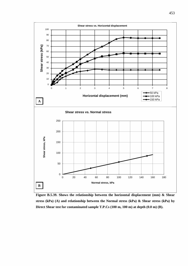
453
Figure B.5.39. Shows the relationship between the horizontal displacement (mm) & Shear
stress (kPa) (A) and relationship between the Normal stress (kPa) & Shear stress (kPa) by
Direct Shear test for contaminated sample T.P.Cs (100 m, 100 m) at depth (0.0 m) (B).
0
10
20
30
40
50
60
70
80
90
100
0 1 2 3 4 5 6 7 8
Sh
ear
stre
ss (
kPa)
Horizontal displacement (mm)
Shear stress vs. Horizontal displacement
50 kPa100 kPa150 kPaA
0
50
100
150
200
250
0 20 40 60 80 100 120 140 160 180
Sh
ear
stre
ss, k
Pa
Normal stress, kPa
Shear stress vs. Normal stress
B

454
Figure B.5.40. Shows the relationship between the horizontal displacement (mm) & Shear
stress (kPa) (A) and relationship between the Normal stress (kPa) & Shear stress (kPa) by
Direct Shear test for contaminated sample T.P.Cs (100 m, 100 m) at depth (0.25 m) (B).
0
20
40
60
80
100
120
0 1 2 3 4 5 6 7 8
Sh
ear
stre
ss (
kPa)
Horizontal displacement (mm)
Shear stress vs. Horizontal displacement
50 kPa100 kPa150 kPaA
0
50
100
150
200
250
0 20 40 60 80 100 120 140 160 180
Sh
ear
stre
ss, k
Pa
Normal stress, kPa
Shear stress vs. Normal stress
B

455
Figure B.5.41. Shows the relationship between the horizontal displacement (mm) & Shear
stress (kPa) (A) and relationship between the Normal stress (kPa) & Shear stress (kPa) by
Direct Shear test for contaminated sample T.P.Cs (100 m, 100 m) at depth (0.5 m) (B).
0
10
20
30
40
50
60
70
80
90
100
0 1 2 3 4 5 6 7 8
Sh
ear
stre
ss (
kPa)
Horizontal displacement (mm)
Shear stress vs. Horizontal displacement
50 kPa100 kPa150 kPaA
0
50
100
150
200
250
0 20 40 60 80 100 120 140 160 180
Sh
ear
stre
ss, k
Pa
Normal stress, kPa
Shear stress vs. Normal stress
B
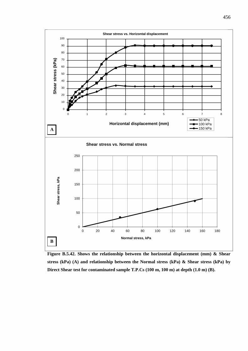
456
Figure B.5.42. Shows the relationship between the horizontal displacement (mm) & Shear
stress (kPa) (A) and relationship between the Normal stress (kPa) & Shear stress (kPa) by
Direct Shear test for contaminated sample T.P.Cs (100 m, 100 m) at depth (1.0 m) (B).
0
10
20
30
40
50
60
70
80
90
100
0 1 2 3 4 5 6 7 8
Sh
ear
stre
ss (
kPa)
Horizontal displacement (mm)
Shear stress vs. Horizontal displacement
50 kPa100 kPa150 kPaA
0
50
100
150
200
250
0 20 40 60 80 100 120 140 160 180
Sh
ear
stre
ss, k
Pa
Normal stress, kPa
Shear stress vs. Normal stress
B

457
Figure B.5.43. Shows the relationship between the horizontal displacement (mm) & Shear
stress (kPa) (A) and relationship between the Normal stress (kPa) & Shear stress (kPa) by
Direct Shear test for contaminated sample T.P.Cs (100 m, 100 m) at depth (1.5 m) (B).
0
20
40
60
80
100
120
0 1 2 3 4 5 6 7 8
Sh
ear
stre
ss (
kPa)
Horizontal displacement (mm)
Shear stress vs. Horizontal displacement
50 kPa100 kPa150 kPaA
0
50
100
150
200
250
0 20 40 60 80 100 120 140 160 180
Sh
ear
stre
ss, k
Pa
Normal stress, kPa
Shear stress vs. Normal stress
B

458
Figure B.5.44. Shows the relationship between the horizontal displacement (mm) & Shear
stress (kPa) (A) and relationship between the Normal stress (kPa) & Shear stress (kPa) by
Direct Shear test for contaminated sample T.P.Cs (100 m, 100 m) at depth (2.0 m) (B).
0
20
40
60
80
100
120
0 1 2 3 4 5 6 7 8
Sh
ear
stre
ss (
kPa)
Horizontal displacement (mm)
Shear stress vs. Horizontal displacement
50 kPa100 kPa150 kPaA
0
50
100
150
200
250
0 20 40 60 80 100 120 140 160 180
Sh
ear
stre
ss (
kPa)
Normal stress (kPa)
Shear stress vs. Normal stress
B
459
Figure B.5.45. Shows the relationship between the horizontal displacement (mm) & Shear
stress (kPa) (A) and relationship between the Normal stress (kPa) & Shear stress (kPa) by
Direct Shear test for non-contaminated sample T.P.Cs (0 m, 0 m) at depth (0.0 m) (B).
0
20
40
60
80
100
120
140
160
180
200
0 0.5 1 1.5 2 2.5
Sh
ear
stre
ss (
kPa)
Horizontal displacement (mm)
Shear stress vs. Horizontal displacement
50 kPa
100 kPa
150 kPa
0
50
100
150
200
250
0 50 100 150 200 250 300
Sh
ear
stre
ss, k
Pa
Normal stress, kPa
Shear stress vs. Normal stress
A
B
460
Figure B.5.46. Shows the relationship between the horizontal displacement (mm) & Shear
stress (kPa) (A) and relationship between the Normal stress (kPa) & Shear stress (kPa) by
Direct Shear test for non-contaminated sample T.P.Cs (0 m, 0 m) at depth (0.25 m) (B).
0
20
40
60
80
100
120
140
160
180
200
0 0.5 1 1.5 2 2.5 3
Sh
ear
stre
ss (
kPa)
Horizontal displacement (mm)
Shear stress vs. Horizontal displacement
50 kPa
100 kPa
150 kPa
0
50
100
150
200
250
0 50 100 150 200 250 300
Sh
ear
stre
ss, k
Pa
Normal stress, kPa
Shear stress vs. Normal stress
A
B

461
Figure B.5.47. Shows the relationship between the horizontal displacement (mm) & Shear
stress (kPa) (A) and relationship between the Normal stress (kPa) & Shear stress (kPa) by
Direct Shear test for non-contaminated sample T.P.Cs (0 m, 0 m) at depth (0.5 m) (B).
0
50
100
150
200
250
0 0.5 1 1.5 2 2.5 3
Sh
ear
stre
ss (
kPa)
Horizontal displacement (mm)
Shear stress vs. Horizontal displacement
50 kPa
100 kPa
150 kPa
0
50
100
150
200
250
0 50 100 150 200 250 300
Sh
ear
stre
ss, k
Pa
Normal stress, kPa
Shear stress vs. Normal stress
A
B
462
Figure B.5.48. Shows the relationship between the horizontal displacement (mm) & Shear
stress (kPa) (A) and relationship between the Normal stress (kPa) & Shear stress (kPa) by
Direct Shear test for non-contaminated sample T.P.Cs (0 m, 0 m) at depth (1.0 m) (B).
0
50
100
150
200
250
0 0.5 1 1.5 2 2.5 3
Sh
ear
stre
ss (
kPa)
Horizontal displacement (mm)
Shear stress vs. Horizontal displacement
50 kPa
100 kPa
150 kPa
0
50
100
150
200
250
0 50 100 150 200 250 300
Sh
ear
stre
ss, k
Pa
Normal stress, kPa
Shear stress vs. Normal stress
A
B
463
Figure B.5.49. Shows the relationship between the horizontal displacement (mm) & Shear
stress (kPa) (A) and relationship between the Normal stress (kPa) & Shear stress (kPa) by
Direct Shear test for non-contaminated sample T.P.Cs (0 m, 0 m) at depth (1.5 m) (B).
0
50
100
150
200
250
0 0.5 1 1.5 2 2.5 3
Sh
ear
stre
ss (
kPa)
Horizontal displacement (mm)
Shear stress vs. Horizontal displacement
50 kPa
100 kPa
150 kPa
0
50
100
150
200
250
0 50 100 150 200 250 300
Sh
ear
stre
ss, k
Pa
Normal stress, kPa
Shear stress vs. Normal stress
A
B
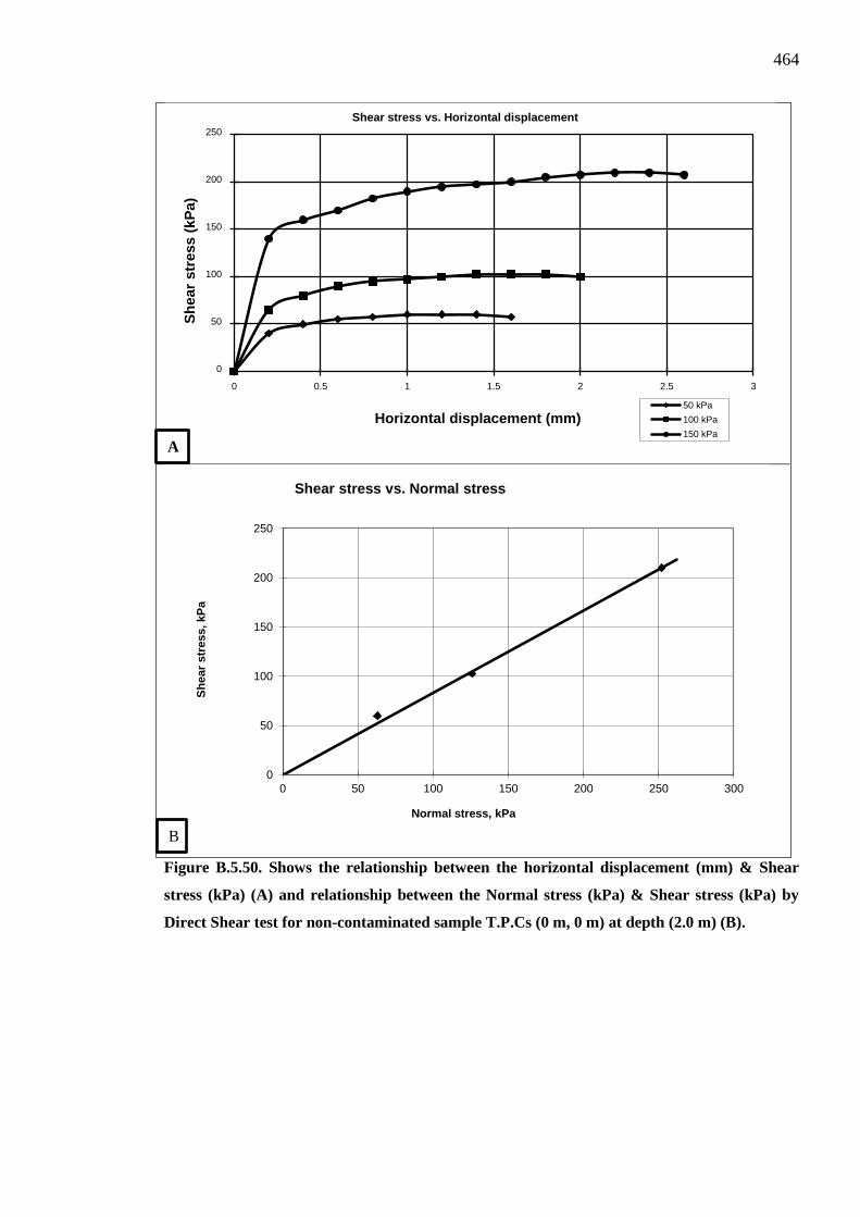
464
Figure B.5.50. Shows the relationship between the horizontal displacement (mm) & Shear
stress (kPa) (A) and relationship between the Normal stress (kPa) & Shear stress (kPa) by
Direct Shear test for non-contaminated sample T.P.Cs (0 m, 0 m) at depth (2.0 m) (B).
0
50
100
150
200
250
0 0.5 1 1.5 2 2.5 3
Sh
ear
stre
ss (
kPa)
Horizontal displacement (mm)
Shear stress vs. Horizontal displacement
50 kPa
100 kPa
150 kPa
0
50
100
150
200
250
0 50 100 150 200 250 300
Sh
ear
stre
ss, k
Pa
Normal stress, kPa
Shear stress vs. Normal stress
A
B
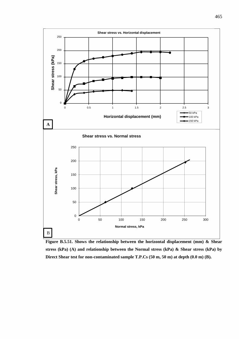
465
Figure B.5.51. Shows the relationship between the horizontal displacement (mm) & Shear
stress (kPa) (A) and relationship between the Normal stress (kPa) & Shear stress (kPa) by
Direct Shear test for non-contaminated sample T.P.Cs (50 m, 50 m) at depth (0.0 m) (B).
0
50
100
150
200
250
0 0.5 1 1.5 2 2.5 3
Sh
ear
stre
ss (
kPa)
Horizontal displacement (mm)
Shear stress vs. Horizontal displacement
50 kPa
100 kPa
150 kPa
0
50
100
150
200
250
0 50 100 150 200 250 300
Sh
ear
stre
ss, k
Pa
Normal stress, kPa
Shear stress vs. Normal stress
A
B
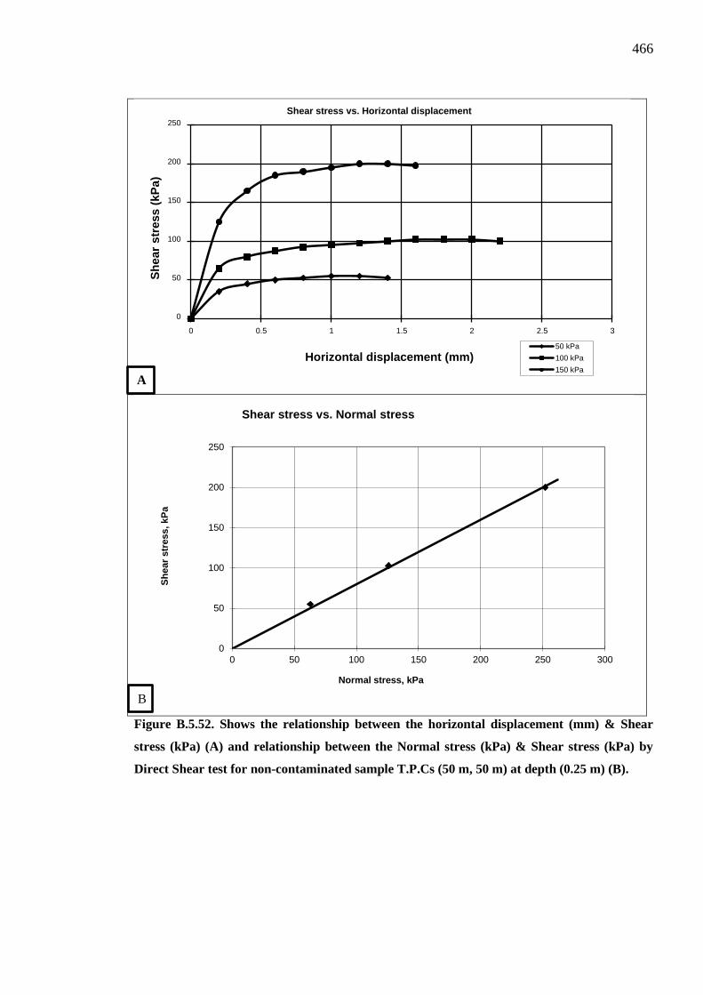
466
Figure B.5.52. Shows the relationship between the horizontal displacement (mm) & Shear
stress (kPa) (A) and relationship between the Normal stress (kPa) & Shear stress (kPa) by
Direct Shear test for non-contaminated sample T.P.Cs (50 m, 50 m) at depth (0.25 m) (B).
0
50
100
150
200
250
0 0.5 1 1.5 2 2.5 3
Sh
ear
stre
ss (
kPa)
Horizontal displacement (mm)
Shear stress vs. Horizontal displacement
50 kPa
100 kPa
150 kPa
0
50
100
150
200
250
0 50 100 150 200 250 300
Sh
ear
stre
ss, k
Pa
Normal stress, kPa
Shear stress vs. Normal stress
A
B

467
Figure B.5.53. Shows the relationship between the horizontal displacement (mm) & Shear
stress (kPa) (A) and relationship between the Normal stress (kPa) & Shear stress (kPa) by
Direct Shear test for non-contaminated sample T.P.Cs (50 m, 50 m) at depth (0.5 m) (B).
0
50
100
150
200
250
0 0.5 1 1.5 2 2.5 3
Sh
ear
stre
ss (
kPa)
Horizontal displacement (mm)
Shear stress vs. Horizontal displacement
50 kPa
100 kPa
150 kPa
0
50
100
150
200
250
0 50 100 150 200 250 300
Sh
ear
stre
ss, k
Pa
Normal stress, kPa
Shear stress vs. Normal stress
A
B

468
Figure B.5.54. Shows the relationship between the horizontal displacement (mm) & Shear
stress (kPa) (A) and relationship between the Normal stress (kPa) & Shear stress (kPa) by
Direct Shear test for non-contaminated sample T.P.Cs (50 m, 50 m) at depth (1.0 m) (B).
0
50
100
150
200
250
0 0.5 1 1.5 2 2.5 3
Sh
ear
stre
ss (
kPa)
Horizontal displacement (mm)
Shear stress vs. Horizontal displacement
50 kPa
100 kPa
150 kPa
0
50
100
150
200
250
0 50 100 150 200 250 300
Sh
ear
stre
ss, k
Pa
Normal stress, kPa
Shear stress vs. Normal stress
A
B

469
Figure B.5.55. Shows the relationship between the horizontal displacement (mm) & Shear
stress (kPa) (A) and relationship between the Normal stress (kPa) & Shear stress (kPa) by
Direct Shear test for non-contaminated sample T.P.Cs (50 m, 50 m) at depth (1.5 m) (B).
0
50
100
150
200
250
0 0.5 1 1.5 2 2.5 3
Sh
ear
stre
ss (
kPa)
Horizontal displacement (mm)
Shear stress vs. Horizontal displacement
50 kPa
100 kPa
150 kPa
0
50
100
150
200
250
0 50 100 150 200 250 300
Sh
ear
stre
ss, k
Pa
Normal stress, kPa
Shear stress vs. Normal stress
A
B
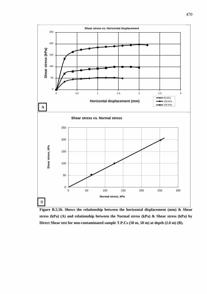
470
Figure B.5.56. Shows the relationship between the horizontal displacement (mm) & Shear
stress (kPa) (A) and relationship between the Normal stress (kPa) & Shear stress (kPa) by
Direct Shear test for non-contaminated sample T.P.Cs (50 m, 50 m) at depth (2.0 m) (B).
0
50
100
150
200
250
0 0.5 1 1.5 2 2.5 3
Sh
ear
stre
ss (
kPa)
Horizontal displacement (mm)
Shear stress vs. Horizontal displacement
50 kPa
100 kPa
150 kPa
0
50
100
150
200
250
0 50 100 150 200 250 300
Sh
ear
stre
ss, k
Pa
Normal stress, kPa
Shear stress vs. Normal stress
A
B

471
Figure B.5.57. Shows the relationship between the horizontal displacement (mm) & Shear
stress (kPa) (A) and relationship between the Normal stress (kPa) & Shear stress (kPa) by
Direct Shear test for non-contaminated sample T.P.Cs (100 m, 100 m) at depth (0.0 m) (B).
0
50
100
150
200
250
0 0.5 1 1.5 2 2.5 3
Sh
ear
stre
ss (
kPa)
Horizontal displacement (mm)
Shear stress vs. Horizontal displacement
50 kPa
100 kPa
150 kPa
0
50
100
150
200
250
0 50 100 150 200 250 300
Sh
ear
stre
ss, k
Pa
Normal stress, kPa
Shear stress vs. Normal stress
A
B

472
Figure B.5.58. Shows the relationship between the horizontal displacement (mm) & Shear
stress (kPa) (A) and relationship between the Normal stress (kPa) & Shear stress (kPa) by
Direct Shear test for non-contaminated sample T.P.Cs (100 m, 100 m) at depth (0.25 m) (B).
0
50
100
150
200
250
0 0.5 1 1.5 2 2.5 3
Sh
ear
stre
ss (
kPa)
Horizontal displacement (mm)
Shear stress vs. Horizontal displacement
50 kPa
100 kPa
150 kPa
0
50
100
150
200
250
0 50 100 150 200 250 300
Sh
ear
stre
ss, k
Pa
Normal stress, kPa
Shear stress vs. Normal stress
A
B

473
Figure B.5.59. Shows the relationship between the horizontal displacement (mm) & Shear
stress (kPa) (A) and relationship between the Normal stress (kPa) & Shear stress (kPa) by
Direct Shear test for non-contaminated sample T.P.Cs (100 m, 100 m) at depth (0.5 m) (B).
0
50
100
150
200
250
0 0.5 1 1.5 2 2.5 3
Sh
ear
stre
ss (
kPa)
Horizontal displacement (mm)
Shear stress vs. Horizontal displacement
50 kPa
100 kPa
150 kPa
0
50
100
150
200
250
0 50 100 150 200 250 300
Sh
ear
stre
ss, k
Pa
Normal stress, kPa
Shear stress vs. Normal stress
A
B
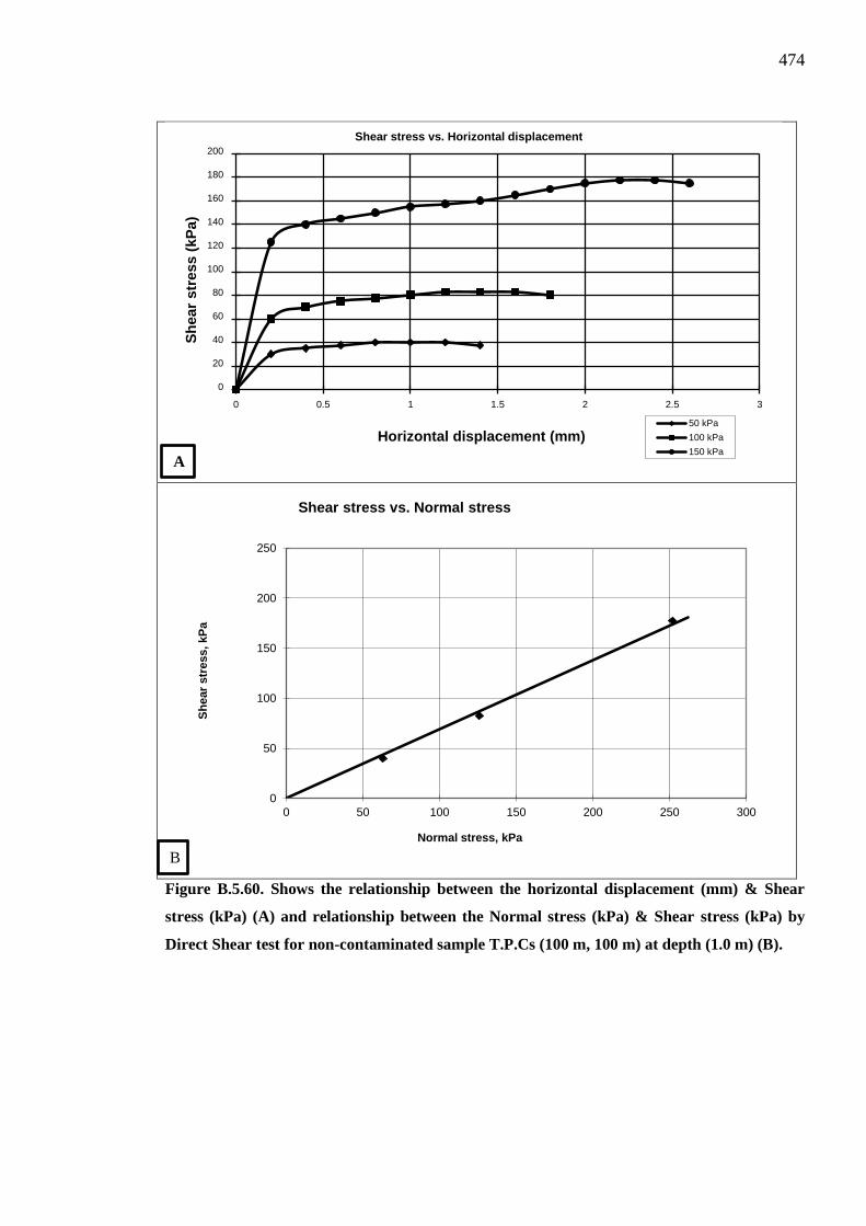
474
Figure B.5.60. Shows the relationship between the horizontal displacement (mm) & Shear
stress (kPa) (A) and relationship between the Normal stress (kPa) & Shear stress (kPa) by
Direct Shear test for non-contaminated sample T.P.Cs (100 m, 100 m) at depth (1.0 m) (B).
0
20
40
60
80
100
120
140
160
180
200
0 0.5 1 1.5 2 2.5 3
Sh
ear
stre
ss (
kPa)
Horizontal displacement (mm)
Shear stress vs. Horizontal displacement
50 kPa
100 kPa
150 kPa
0
50
100
150
200
250
0 50 100 150 200 250 300
Sh
ear
stre
ss, k
Pa
Normal stress, kPa
Shear stress vs. Normal stress
A
B

475
Figure B.5.61. Shows the relationship between the horizontal displacement (mm) & Shear
stress (kPa) (A) and relationship between the Normal stress (kPa) & Shear stress (kPa) by
Direct Shear test for non-contaminated sample T.P.Cs (100 m, 100 m) at depth (1.5 m) (B).
0
20
40
60
80
100
120
140
160
180
200
0 0.5 1 1.5 2 2.5 3
Sh
ear
stre
ss (
kPa)
Horizontal displacement (mm)
Shear stress vs. Horizontal displacement
50 kPa
100 kPa
150 kPa
0
50
100
150
200
250
0 50 100 150 200 250 300
Sh
ear
stre
ss, k
Pa
Normal stress, kPa
Shear stress vs. Normal stress
A
B
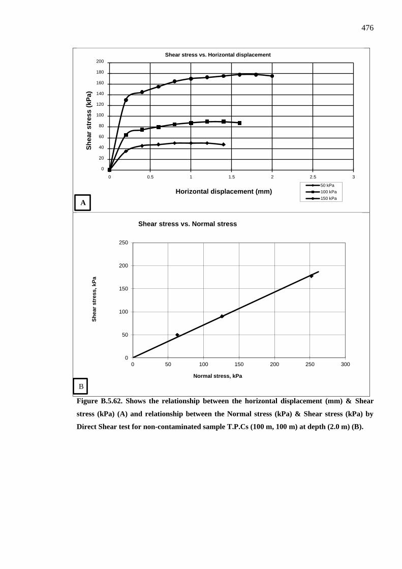
476
Figure B.5.62. Shows the relationship between the horizontal displacement (mm) & Shear
stress (kPa) (A) and relationship between the Normal stress (kPa) & Shear stress (kPa) by
Direct Shear test for non-contaminated sample T.P.Cs (100 m, 100 m) at depth (2.0 m) (B).
0
20
40
60
80
100
120
140
160
180
200
0 0.5 1 1.5 2 2.5 3
Sh
ear
stre
ss (
kPa)
Horizontal displacement (mm)
Shear stress vs. Horizontal displacement
50 kPa
100 kPa
150 kPa
0
50
100
150
200
250
0 50 100 150 200 250 300
Sh
ear
stre
ss, k
Pa
Normal stress, kPa
Shear stress vs. Normal stress
A
B

477
Table B.5.26. The significant p-values via normality Shapiro-Wilk test indicate that the angle of internal friction (φ) values of the soil at contaminated and non-contaminated sites follow normal distribution.
Table B.5.27. Indicates the significant differences of the angle of internal friction (φ) variable in the soil at six different depths between contaminated and non-contaminated sites.
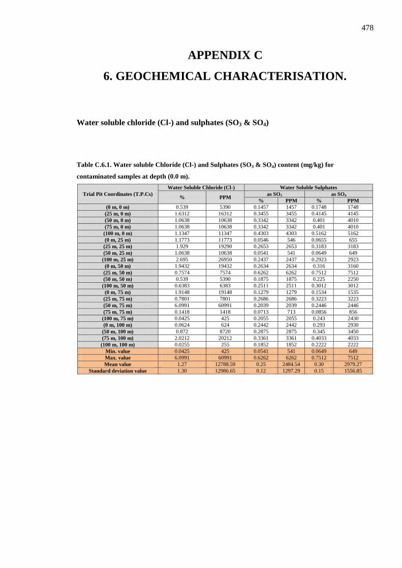
478
APPENDIX C
6. GEOCHEMICAL CHARACTERISATION.
Water soluble chloride (Cl-) and sulphates (SO3 & SO4)
Table C.6.1. Water soluble Chloride (Cl-) and Sulphates (SO3 & SO4) content (mg/kg) for
contaminated samples at depth (0.0 m).
Trial Pit Coordinates (T.P.Cs) Water Soluble Chloride (Cl-) Water Soluble Sulphates
% PPM as SO3 as SO4
% PPM % PPM (0 m, 0 m) 0.539 5390 0.1457 1457 0.1748 1748 (25 m, 0 m) 1.6312 16312 0.3455 3455 0.4145 4145 (50 m, 0 m) 1.0638 10638 0.3342 3342 0.401 4010 (75 m, 0 m) 1.0638 10638 0.3342 3342 0.401 4010
(100 m, 0 m) 1.1347 11347 0.4303 4303 0.5162 5162 (0 m, 25 m) 1.1773 11773 0.0546 546 0.0655 655
(25 m, 25 m) 1.929 19290 0.2653 2653 0.3183 3183 (50 m, 25 m) 1.0638 10638 0.0541 541 0.0649 649
(100 m, 25 m) 2.695 26950 0.2437 2437 0.2923 2923 (0 m, 50 m) 1.9432 19432 0.2634 2634 0.316 3160
(25 m, 50 m) 0.7574 7574 0.6262 6262 0.7512 7512 (50 m, 50 m) 0.539 5390 0.1875 1875 0.225 2250
(100 m, 50 m) 0.6383 6383 0.2511 2511 0.3012 3012 (0 m, 75 m) 1.9148 19148 0.1279 1279 0.1534 1535
(25 m, 75 m) 0.7801 7801 0.2686 2686 0.3223 3223 (50 m, 75 m) 6.0991 60991 0.2039 2039 0.2446 2446 (75 m, 75 m) 0.1418 1418 0.0713 713 0.0856 856
(100 m, 75 m) 0.0425 425 0.2055 2055 0.243 2430 (0 m, 100 m) 0.0624 624 0.2442 2442 0.293 2930
(50 m, 100 m) 0.872 8720 0.2875 2875 0.345 3450 (75 m, 100 m) 2.0212 20212 0.3361 3361 0.4033 4033 (100 m, 100 m) 0.0255 255 0.1852 1852 0.2222 2222
Min. value 0.0425 425 0.0541 541 0.0649 649 Max. value 6.0991 60991 0.6262 6262 0.7512 7512 Mean value 1.27 12788.59 0.25 2484.54 0.30 2979.27
Standard deviation value 1.30 12986.65 0.12 1297.29 0.15 1556.85

479
Table C.6.2. Water soluble Chloride (Cl-) and Sulphates (SO3 & SO4) content (mg/kg) for
contaminated samples at depth (0.25 m).
Trial Pit Coordinates (T.P.Cs) Water Soluble Chloride (Cl-) Water Soluble Sulphates
% PPM as SO3 as SO4
% PPM % PPM (0 m, 0 m) 0.0851 851 0.0568 568 0.0681 681
(25 m, 0 m) 0.5674 5674 0.1583 1583 0.1899 1899 (50 m, 0 m) 0.2837 2837 0.0527 527 0.0632 632 (75 m, 0 m) 1.5248 15248 0.1026 1026 0.1231 1231 (100 m, 0 m) 0.1986 1986 0.0156 156 0.0188 188 (0 m, 25 m) 0.5674 5674 0.2733 2733 0.3279 3279 (25 m, 25 m) 0.2695 2695 0.0211 211 0.0253 253 (50 m, 25 m) 0.2128 2128 0.0206 206 0.0247 247
(100 m, 25 m) 0.6737 6737 0.0288 288 0.0346 346 (0 m, 50 m) 3.8297 38297 0.2629 2629 0.3154 3154 (25 m, 50 m) 0.8794 8794 0.261 2610 0.3131 3131 (50 m, 50 m) 0.539 5390 0.1875 1875 0.225 2250
(100 m, 50 m) 0.0709 709 0.0615 615 0.0737 737 (0 m, 75 m) 3.9006 39006 0.0129 129 0.0155 155 (25 m, 75 m) 0.4964 4964 0.1196 1196 0.1435 1435 (50 m, 75 m) 0.3546 3546 0.0617 617 0.0741 741 (75 m, 75 m) 0.695 6950 0.197 1970 0.2364 2364
(100 m, 75 m) 0.0055 55 0.189 1890 0.2268 2268 (0 m, 100 m) 0.0975 975 0.1207 1207 0.1448 1448
(50 m, 100 m) 0.1418 1418 0.0847 847 0.1017 1017 (75 m, 100 m) 4.0779 40779 0.2582 2582 0.3098 3098
(100 m, 100 m) 0.0043 43 0.2009 2009 0.241 2410 Min. value 0.0043 43 0.0129 129 0.0155 155 Max. value 4.077 40779 0.2733 2733 0.3279 3279 Mean value 0.885 8852.545 0.1248 1248.818 0.1498 1498.363
Standard deviation value 1.288 12889.877 0.090 907.319 0.1088 1088.522
Table C.6.3. Water soluble Chloride (Cl-) and Sulphates (SO3 & SO4) content (mg/kg) for
contaminated samples at depth (0.5 m).
Trial Pit Coordinates (T.P.Cs) Water Soluble Chloride (Cl-) Water Soluble Sulphates
% PPM as SO3 as SO4
% PPM % PPM (0 m, 0 m) 0.0426 426 0.084 840 0.1007 1007 (25 m, 0 m) 0.2695 2695 0.0255 255 0.0306 306 (50 m, 0 m) 0.2837 2837 0.0104 104 0.0125 125 (75 m, 0 m) 0.2837 2837 0.0104 104 0.0125 125
(100 m, 0 m) 0.0284 284 0.0154 154 0.0184 184 (0 m, 25 m) 2.0567 20567 0.1583 1583 0.1899 1899
(25 m, 25 m) 0.0709 709 0.0436 436 0.0523 523 (50 m, 25 m) 0.0851 851 0.0184 184 0.0221 221
(100 m, 25 m) 0.3262 3262 0.0104 104 0.0125 125 (0 m, 50 m) 0.4681 4681 0.022 220 0.0263 263
(25 m, 50 m) 0.2553 2553 0.0132 131 0.0158 158 (50 m, 50 m) 0.0552 552 0.0971 971 0.1165 1165
(100 m, 50 m) 0.4964 4964 0.1117 1117 0.134 1340 (0 m, 75 m) 2.5531 25531 0.0198 198 0.0237 237
(25 m, 75 m) 0.2837 2837 0.1767 1767 0.212 212 (50 m, 75 m) 0.3546 3546 0.2187 2187 0.2624 2624 (75 m, 75 m) 0.1418 1418 0.0252 252 0.0303 303
(100 m, 75 m) 0.0085 85 0.1876 1876 0.2251 2251 (0 m, 100 m) 0.0283 283 0.2025 2025 0.243 2430
(50 m, 100 m) 0.0082 82 0.1033 1033 0.124 1240 (75 m, 100 m) 0.7518 7518 0.0255 255 0.0306 306 (100 m, 100 m) 0.0043 43 0.1583 1583 0.1899 1899
Min. value 0.0082 82 0.0104 104 0.0125 125 Max. value 2.553 25531 0.2187 2187 0.262 2624 Mean value 0.402 4025.5 0.079 789.95 0.094 861.045
Standard deviation value 0.649 6497.054 0.073 735.17 0.088 854.701

480
Table C.6.4. Water soluble Chloride (Cl-) and Sulphates (SO3 & SO4) content for contaminated
samples at depth (1.0 m).
Trial Pit Coordinates (T.P.Cs) Water Soluble Chloride (Cl-) Water Soluble Sulphates
% PPM as SO3 as SO4
% PPM % PPM (0 m, 0 m) 0.3972 3972 0.0768 768 0.0922 922
(25 m, 0 m) 0.2269 2269 0.0184 184 0.0221 221 (50 m, 0 m) 0.4397 4397 0.0096 96 0.0115 115 (75 m, 0 m) 0.4397 4397 0.0096 96 0.0115 115 (100 m, 0 m) 0.1135 1135 0.0115 115 0.0138 138 (0 m, 25 m) 1.4184 14184 0.1106 1106 0.1327 1327 (25 m, 25 m) 0.1277 1277 0.0392 392 0.0471 471 (50 m, 25 m) 0.0993 993 0.0091 91 0.0109 109
(100 m, 25 m) 0.1702 1702 0.0195 195 0.0234 234 (0 m, 50 m) 0.6525 6525 0.022 220 0.0263 263 (25 m, 50 m) 0.1986 1986 0.0027 27 0.0033 33 (50 m, 50 m) 0.1037 1037 0.067 670 0.0804 804
(100 m, 50 m) 0.1475 1475 0.2247 2247 0.2696 2696 (0 m, 75 m) 0.922 9220 0.1495 1495 0.1794 1795 (25 m, 75 m) 0.1844 1844 0.0519 519 0.0622 622 (50 m, 75 m) 0.3546 3546 0.1841 1841 0.2209 2209 (75 m, 75 m) 0.1986 1986 0.1402 1402 0.1682 1682
(100 m, 75 m) 0.0556 556 0.088 880 0.1056 1056 (0 m, 100 m) 0.1673 1673 0.0274 274 0.0329 329
(50 m, 100 m) 0.0237 237 0.0567 567 0.068 680 (75 m, 100 m) 1.078 10780 0.0541 541 0.0649 649
(100 m, 100 m) 0.0085 85 0.0291 291 0.0349 349 Min. value 0.008 85 0.0027 27 0.0033 33 Max. value 1.418 14184 0.224 2247 0.2696 2696 Mean value 0.342 3421.636 0.0637 637.136 0.076 764.5
Standard deviation value 0.367 3678.060 0.062 621.152 0.074 745.37
Table C.6.5. Water soluble Chloride (Cl-) and Sulphates (SO3 & SO4) content (mg/kg) for
contaminated samples at depth (1.5 m).
Trial Pit Coordinates (T.P.Cs) Water Soluble Chloride (Cl-) Water Soluble Sulphates
% PPM as SO3 as SO4
% PPM % PPM (0 m, 0 m) 0.3404 3404 0.045 450 0.054 540 (25 m, 0 m) 0.1277 1277 0.0085 85 0.0102 102 (50 m, 0 m) 0.1702 1702 0.0134 134 0.0161 161 (75 m, 0 m) 0.1702 1702 0.0134 134 0.0161 161
(100 m, 0 m) 0.1702 1702 0.0107 107 0.0128 128 (0 m, 25 m) 0.9929 9929 0.0702 702 0.0843 843
(25 m, 25 m) 0.1418 1418 0.0239 239 0.0286 286 (50 m, 25 m) 0.1277 1277 0.0104 104 0.0125 125
(100 m, 25 m) 0.2411 2411 0.0184 184 0.0221 221 (0 m, 50 m) 0.2553 2553 0.0121 121 0.0145 145
(25 m, 50 m) 0.2128 2128 0.0005 5 0.0007 7 (50 m, 50 m) 0.023 230 0.1422 1422 0.1706 1706
(100 m, 50 m) 0.4255 4255 0.0154 154 0.0184 184 (0 m, 75 m) 0.851 8510 0.053 530 0.0635 635
(25 m, 75 m) 0.312 3120 0.0214 214 0.0257 257 (50 m, 75 m) 0.3546 3546 0.1841 1841 0.2209 2209 (75 m, 75 m) 0.2695 2695 0.0228 228 0.0273 273
(100 m, 75 m) 0.0228 228 0.029 290 0.0348 348 (0 m, 100 m) 0.0936 936 0.1009 1009 0.1211 1211
(50 m, 100 m) 0.0208 208 0.145 1450 0.174 1740 (75 m, 100 m) 0.1986 1986 0.0524 524 0.0629 629 (100 m, 100 m) 0.0085 85 0.0656 656 0.0787 787
Min. value 0.008 85 0.0005 5 0.0007 7 Max. value 0.992 9929 0.184 1841 0.220 2209 Mean value 0.251 2513.727 0.048 481.04 0.057 577.181
Standard deviation value 0.245 2459.695 0.05 511.71 0.061 614.009
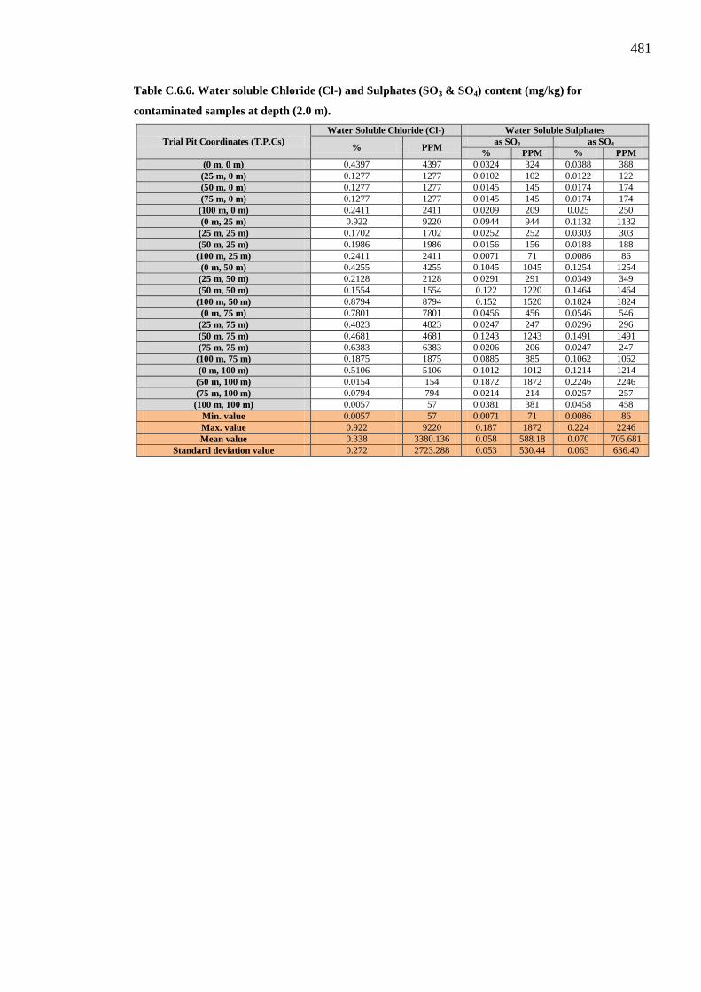
481
Table C.6.6. Water soluble Chloride (Cl-) and Sulphates (SO3 & SO4) content (mg/kg) for
contaminated samples at depth (2.0 m).
Trial Pit Coordinates (T.P.Cs) Water Soluble Chloride (Cl-) Water Soluble Sulphates
% PPM as SO3 as SO4
% PPM % PPM (0 m, 0 m) 0.4397 4397 0.0324 324 0.0388 388 (25 m, 0 m) 0.1277 1277 0.0102 102 0.0122 122 (50 m, 0 m) 0.1277 1277 0.0145 145 0.0174 174 (75 m, 0 m) 0.1277 1277 0.0145 145 0.0174 174
(100 m, 0 m) 0.2411 2411 0.0209 209 0.025 250 (0 m, 25 m) 0.922 9220 0.0944 944 0.1132 1132
(25 m, 25 m) 0.1702 1702 0.0252 252 0.0303 303 (50 m, 25 m) 0.1986 1986 0.0156 156 0.0188 188
(100 m, 25 m) 0.2411 2411 0.0071 71 0.0086 86 (0 m, 50 m) 0.4255 4255 0.1045 1045 0.1254 1254
(25 m, 50 m) 0.2128 2128 0.0291 291 0.0349 349 (50 m, 50 m) 0.1554 1554 0.122 1220 0.1464 1464
(100 m, 50 m) 0.8794 8794 0.152 1520 0.1824 1824 (0 m, 75 m) 0.7801 7801 0.0456 456 0.0546 546
(25 m, 75 m) 0.4823 4823 0.0247 247 0.0296 296 (50 m, 75 m) 0.4681 4681 0.1243 1243 0.1491 1491 (75 m, 75 m) 0.6383 6383 0.0206 206 0.0247 247
(100 m, 75 m) 0.1875 1875 0.0885 885 0.1062 1062 (0 m, 100 m) 0.5106 5106 0.1012 1012 0.1214 1214
(50 m, 100 m) 0.0154 154 0.1872 1872 0.2246 2246 (75 m, 100 m) 0.0794 794 0.0214 214 0.0257 257 (100 m, 100 m) 0.0057 57 0.0381 381 0.0458 458
Min. value 0.0057 57 0.0071 71 0.0086 86 Max. value 0.922 9220 0.187 1872 0.224 2246 Mean value 0.338 3380.136 0.058 588.18 0.070 705.681
Standard deviation value 0.272 2723.288 0.053 530.44 0.063 636.40
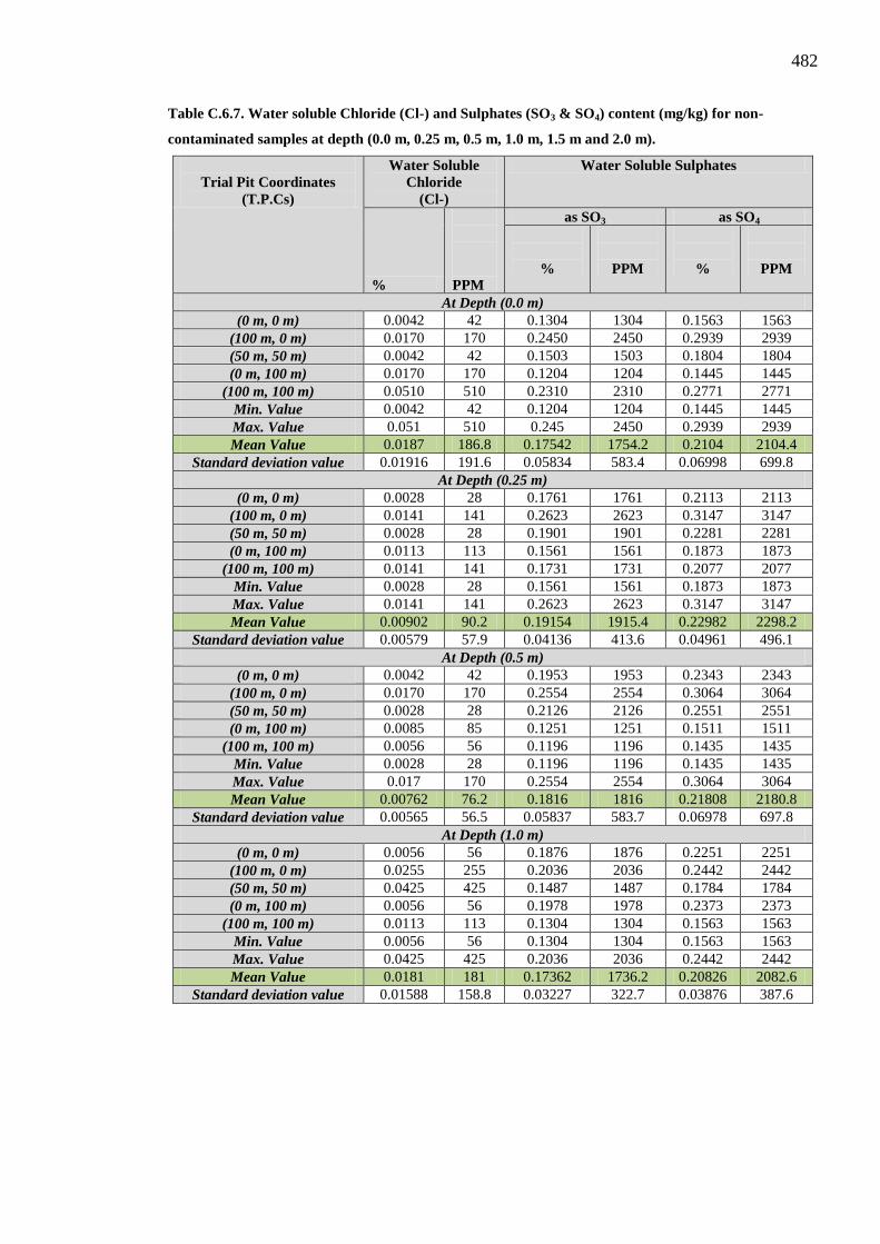
482
Table C.6.7. Water soluble Chloride (Cl-) and Sulphates (SO3 & SO4) content (mg/kg) for non-
contaminated samples at depth (0.0 m, 0.25 m, 0.5 m, 1.0 m, 1.5 m and 2.0 m).
Trial Pit Coordinates
(T.P.Cs)
Water Soluble Chloride
(Cl-)
Water Soluble Sulphates
%
PPM
as SO3 as SO4
%
PPM
%
PPM
At Depth (0.0 m) (0 m, 0 m) 0.0042 42 0.1304 1304 0.1563 1563
(100 m, 0 m) 0.0170 170 0.2450 2450 0.2939 2939 (50 m, 50 m) 0.0042 42 0.1503 1503 0.1804 1804 (0 m, 100 m) 0.0170 170 0.1204 1204 0.1445 1445
(100 m, 100 m) 0.0510 510 0.2310 2310 0.2771 2771 Min. Value 0.0042 42 0.1204 1204 0.1445 1445 Max. Value 0.051 510 0.245 2450 0.2939 2939 Mean Value 0.0187 186.8 0.17542 1754.2 0.2104 2104.4
Standard deviation value 0.01916 191.6 0.05834 583.4 0.06998 699.8 At Depth (0.25 m)
(0 m, 0 m) 0.0028 28 0.1761 1761 0.2113 2113 (100 m, 0 m) 0.0141 141 0.2623 2623 0.3147 3147 (50 m, 50 m) 0.0028 28 0.1901 1901 0.2281 2281 (0 m, 100 m) 0.0113 113 0.1561 1561 0.1873 1873
(100 m, 100 m) 0.0141 141 0.1731 1731 0.2077 2077 Min. Value 0.0028 28 0.1561 1561 0.1873 1873 Max. Value 0.0141 141 0.2623 2623 0.3147 3147 Mean Value 0.00902 90.2 0.19154 1915.4 0.22982 2298.2
Standard deviation value 0.00579 57.9 0.04136 413.6 0.04961 496.1 At Depth (0.5 m)
(0 m, 0 m) 0.0042 42 0.1953 1953 0.2343 2343 (100 m, 0 m) 0.0170 170 0.2554 2554 0.3064 3064 (50 m, 50 m) 0.0028 28 0.2126 2126 0.2551 2551 (0 m, 100 m) 0.0085 85 0.1251 1251 0.1511 1511
(100 m, 100 m) 0.0056 56 0.1196 1196 0.1435 1435 Min. Value 0.0028 28 0.1196 1196 0.1435 1435 Max. Value 0.017 170 0.2554 2554 0.3064 3064 Mean Value 0.00762 76.2 0.1816 1816 0.21808 2180.8
Standard deviation value 0.00565 56.5 0.05837 583.7 0.06978 697.8 At Depth (1.0 m)
(0 m, 0 m) 0.0056 56 0.1876 1876 0.2251 2251 (100 m, 0 m) 0.0255 255 0.2036 2036 0.2442 2442 (50 m, 50 m) 0.0425 425 0.1487 1487 0.1784 1784 (0 m, 100 m) 0.0056 56 0.1978 1978 0.2373 2373
(100 m, 100 m) 0.0113 113 0.1304 1304 0.1563 1563 Min. Value 0.0056 56 0.1304 1304 0.1563 1563 Max. Value 0.0425 425 0.2036 2036 0.2442 2442 Mean Value 0.0181 181 0.17362 1736.2 0.20826 2082.6
Standard deviation value 0.01588 158.8 0.03227 322.7 0.03876 387.6
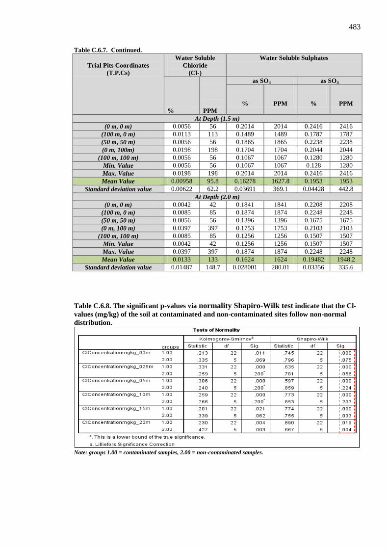
483
Table C.6.7. Continued.
Trial Pits Coordinates (T.P.Cs)
Water Soluble Chloride
(Cl-)
Water Soluble Sulphates
%
PPM
as SO3 as SO4
%
PPM
%
PPM
At Depth (1.5 m) (0 m, 0 m) 0.0056 56 0.2014 2014 0.2416 2416
(100 m, 0 m) 0.0113 113 0.1489 1489 0.1787 1787 (50 m, 50 m) 0.0056 56 0.1865 1865 0.2238 2238 (0 m, 100m) 0.0198 198 0.1704 1704 0.2044 2044
(100 m, 100 m) 0.0056 56 0.1067 1067 0.1280 1280 Min. Value 0.0056 56 0.1067 1067 0.128 1280 Max. Value 0.0198 198 0.2014 2014 0.2416 2416 Mean Value 0.00958 95.8 0.16278 1627.8 0.1953 1953
Standard deviation value 0.00622 62.2 0.03691 369.1 0.04428 442.8 At Depth (2.0 m)
(0 m, 0 m) 0.0042 42 0.1841 1841 0.2208 2208 (100 m, 0 m) 0.0085 85 0.1874 1874 0.2248 2248 (50 m, 50 m) 0.0056 56 0.1396 1396 0.1675 1675 (0 m, 100 m) 0.0397 397 0.1753 1753 0.2103 2103
(100 m, 100 m) 0.0085 85 0.1256 1256 0.1507 1507 Min. Value 0.0042 42 0.1256 1256 0.1507 1507 Max. Value 0.0397 397 0.1874 1874 0.2248 2248 Mean Value 0.0133 133 0.1624 1624 0.19482 1948.2
Standard deviation value 0.01487 148.7 0.028001 280.01 0.03356 335.6
Table C.6.8. The significant p-values via normality Shapiro-Wilk test indicate that the Cl- values (mg/kg) of the soil at contaminated and non-contaminated sites follow non-normal distribution.
Note: groups 1.00 = contaminated samples, 2.00 = non-contaminated samples.

484
Table C.6.9. The significant p-values via normality Shapiro-Wilk test indicate that the SO3 and SO4 values of the soil at contaminated and non-contaminated sites follow normal distribution.
Note: groups 1.00 = contaminated samples, 2.00 = non-contaminated samples. Table C.6.10. Indicates the significant differences of the Cl- (mg/kg) variable in the soil at six different depths between contaminated and non-contaminated sites.

485
Table C.6.11. Indicates the significant differences of the SO3 and SO4 (mg/kg) variables in the soil at six different depths between contaminated and non-contaminated sites.
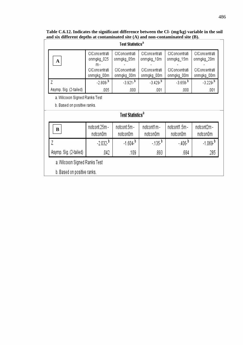
486
Table C.6.12. Indicates the significant difference between the Cl- (mg/kg) variable in the soil and six different depths at contaminated site (A) and non-contaminated site (B).
A
B

487
Elemental Analysis (EA)
Table C.6.13. The percentages (%) results of Nitrogen, Carbon, Sulphur and Hydrogen for
contaminated samples at depth (0.0 m).
Table C.6.14. The percentages (%) results of Nitrogen, Carbon, Sulphur and Hydrogen for
contaminated samples at depth (0.25 m).
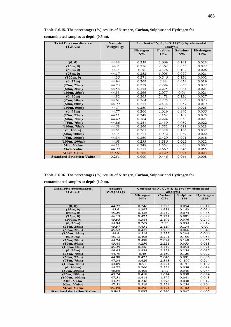
488
Table C.6.15. The percentages (%) results of Nitrogen, Carbon, Sulphur and Hydrogen for
contaminated samples at depth (0.5 m).
Table C.6.16. The percentages (%) results of Nitrogen, Carbon, Sulphur and Hydrogen for
contaminated samples at depth (1.0 m).
489
Table C.6.17. The percentages (%) results of Nitrogen, Carbon, Sulphur and Hydrogen for
contaminated samples at depth (1.5 m).
Table C.6.18. The percentages (%) results of Nitrogen, Carbon, Sulphur and Hydrogen for
contaminated samples at depth (2.0 m).
490
Table C.6.19. The percentages (%) results of Nitrogen, Carbon, Sulphur and Hydrogen for non-
contaminated samples at depths (0.0 m, 0.25 m).
Trial Pits Coordinates. (T.P.Cs)
Sample Weight (g)
Content of N, C, S & H (%) by elemental analysis Nitrogen
N% Carbon
C% Sulphur
S% Hydrogen
H% At Depth (0.0 m)
(0 m, 0 m) 45.940 0.0030 0.011 0.013 0.0052 (100 m, 0 m) 45.160 0.0015 0.021 0.014 0.010 (50 m, 50 m) 44.300 0.0025 0.036 0.004 0.003 (0 m, 100 m) 44.260 0.0029 0.080 0.008 0.0028
(100 m, 100 m) 4.290 0.0037 0.092 0.001 0.0062 Min. value 44.26 0.0015 0.011 0.001 0.0028 Max. value 45.94 0.0037 0.092 0.014 0.01 Mean value 36.79 0.002 0.048 0.008 0.005
Standard deviation value 18.181 0.0008 0.036 0.005 0.002 At Depth (0.25 m)
(0 m, 0 m) 44.130 0.0012 0.001 0.000 0.0001 (100 m, 0 m) 44.810 0.0001 0.000 0.003 0.001 (50 m, 50 m) 44.410 0.000 0.0011 0.000 0.0021 (0 m, 100 m) 45.290 0.000 0.0012 0.002 0.0017
(100 m, 100 m) 46.190 0.000 0.000 0.000 0.0010 Min. value 44.13 0 0 0 0.0001 Max. value 44.81 0.0012 0.0012 0.003 0.0021 Mean value 44.966 0.0002 0.0006 0.001 0.0011
Standard deviation value 0.811 0.0005 0.0006 0.0014 0.0007
491
Table C.6.20. The significant p-values via normality Shapiro-Wilk test indicate that the elemental analysis (i.e. N % (A), C % (B) & S % (C)) values of the soil at contaminated and non-contaminated sites at two different depths (0.0 m & 0.25 m) follow normal distribution.
Table C.6.21. The significant p-values via normality Shapiro-Wilk test indicate that the elemental analysis (i.e. H %) values of the soil at contaminated and non-contaminated sites at two different depths (0.0 m & 0.25 m) follow non-normal distribution.
Note: the H % values at non-contaminated site (group = 2.0) were found to be close to zero.
A A
B B
C

492
Table C.6.22. Indicates the significant differences of the elemental analysis (i.e. N % (A), C % (B) & S % (C)) variables in the soil at two different depths between contaminated and non-contaminated sites.
Table C.6.23. Indicates the significant differences of the elemental analysis (i.e. H %) variable in the soil at two different depths between contaminated and non-contaminated sites.
A
B
C

493
Table C.6.24. Indicates the significant difference between the H % variable in the soil and six different depths at contaminated site.

494
GC-MS Results
495
Table C.6.25. The results of detected soil sample with TPH which tested by GC-MS instrument for T.P.C. (75 m, 0 m) at depth (0.0 m) of contaminated site (Al-Magwa Area).
Peak Ret. Time Chemical Composition of
the TPH in the Contaminated Soil Sample
Area Under the
Curve (m2)
Chemical Composition
Formula
Classification of the
TPH based on Aliphatic and Aromatic
Concentration of each TPH
Chemical Composition
Detected in the Contaminated
Soil Sample (µg/ml)
Concentration of each TPH
Chemical Composition
Detected in the Contaminated
Soil Sample (mg/kg)
Total
Concentration of the Total
TPH Compositions
Detected in the Contaminated
Soil Sample (mg/kg)
References
*1 3.118 BV Dihydroxydimethylsilane -39496627 C2H8O2 ------- 0 0
53.02
(Dimethylsilanediol, n.d.)
**2 19.564 BV BHT 5772938 C15H24
Aromatic EC12 - EC16
48.131 16.043 (BHT, n.d.)
***3 22.458 PV ------ 3018562 ------ ---------
12.462 4.154 ---------
**4 22.575 VV Dihydro indol-2-one 4227389 C8H7NO Aromatic EC8 - EC10 28.116 9.372
(Oxindole, n.d.)
***5 22.901 VV ------ 2078641 ------ ------- 0.290 0.096 ---------
**6 23.077 VV 9,10-Dimethylanthracene 4000251 C16H14 Aromatic EC16- EC21 25.175 8.391 (Nine, 10-
dimethylanthracene, n.d.)
**7 23.191 VV 1,7-Dimethylphenanthrene 5289993 C16H14 Aromatic EC16- EC21 41.877 13.959 (One, 7-
Dimethylphenanthrene, n.d.)
**8 23.337 VV 14β-pregnane 2164912 C21H36 Aliphatic EC16 - EC35 1.407 0.469 ((14β)-Pregnane, n.d.)
**9 23.696 PV Isopentyltrimethyl benezene 3164712 C14H22 Aromatic EC12 - EC16 14.355 4.785
(One-Isopentyl-2,3,5-trimethylbenzene, n.d.)
Notes: * Greeen colure clarify the solvent compound came from the column bleeding during soil sample analysis by GC-MS test. **Brown colour clarify the hydrocarbon compounds and their concentrations detected in soil sample.
***Blue Colure clarify the unknown chemical compounds and their concentrations (not identify by diesel standard) detected in soil sample which are excluded from the total concentration of the TPH.

496
Figure C.6.1. The Total Ion Chromatograms (TIC) of detected soil sample with TPH for T.P.C. (75 m, 0 m) at depth (0.0 m), at contaminated site
(Al-Magwa Area).
5 . 0 0 1 0 . 0 0 1 5 . 0 0 2 0 . 0 0 2 5 . 0 0 3 0 . 0 0 3 5 . 0 0
5 0 0 0 0 0
1 0 0 0 0 0 0
1 5 0 0 0 0 0
2 0 0 0 0 0 0
2 5 0 0 0 0 0
3 0 0 0 0 0 0
3 5 0 0 0 0 0
4 0 0 0 0 0 0
4 5 0 0 0 0 0
T i m e - - >
A b u n d a n c e
T I C : H S 8 9 . D \ d a t a . m s
3 . 1 1 81 9 . 5 6 4
2 2 . 4 5 82 2 . 5 7 52 2 . 9 0 12 3 . 0 7 72 3 . 1 9 12 3 . 3 3 7
2 3 . 6 9 6
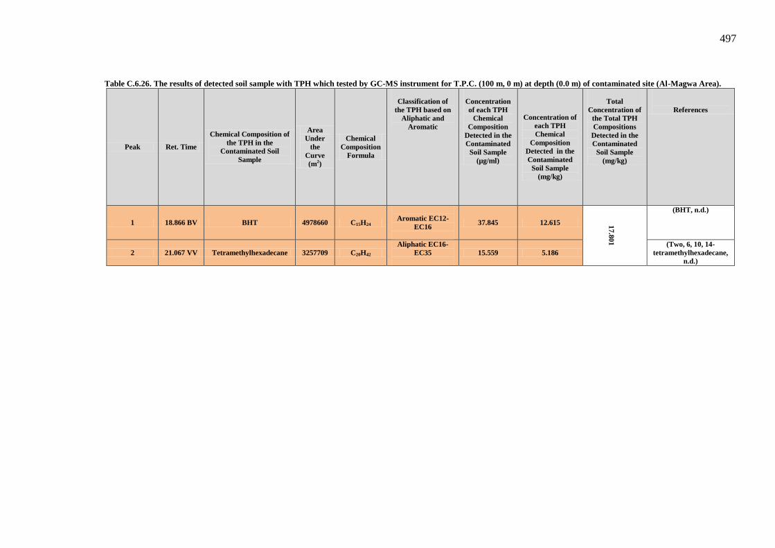
497
Table C.6.26. The results of detected soil sample with TPH which tested by GC-MS instrument for T.P.C. (100 m, 0 m) at depth (0.0 m) of contaminated site (Al-Magwa Area).
Peak Ret. Time
Chemical Composition of the TPH in the
Contaminated Soil Sample
Area Under
the Curve (m2)
Chemical Composition
Formula
Classification of
the TPH based on Aliphatic and
Aromatic
Concentration of each TPH
Chemical Composition
Detected in the Contaminated
Soil Sample (µg/ml)
Concentration of each TPH Chemical
Composition Detected in the Contaminated
Soil Sample (mg/kg)
Total
Concentration of the Total TPH Compositions
Detected in the Contaminated
Soil Sample (mg/kg)
References
1 18.866 BV BHT 4978660 C15H24
Aromatic EC12-
EC16
37.845 12.615
17.801
(BHT, n.d.)
2 21.067 VV Tetramethylhexadecane 3257709 C20H42 Aliphatic EC16-
EC35
15.559 5.186 (Two, 6, 10, 14-
tetramethylhexadecane, n.d.)
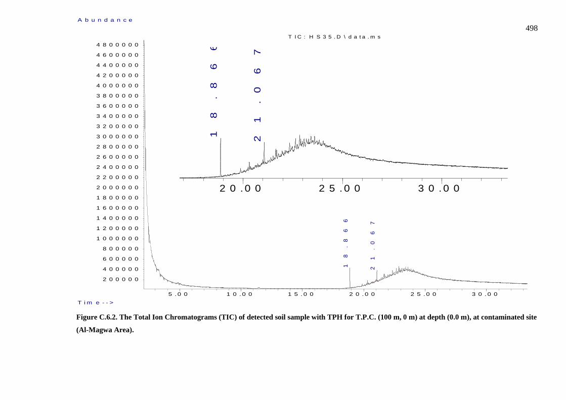
498
Figure C.6.2. The Total Ion Chromatograms (TIC) of detected soil sample with TPH for T.P.C. (100 m, 0 m) at depth (0.0 m), at contaminated site
(Al-Magwa Area).
5 .0 0 1 0 . 0 0 1 5 . 0 0 2 0 . 0 0 2 5 . 0 0 3 0 . 0 0
2 0 0 0 0 0
4 0 0 0 0 0
6 0 0 0 0 0
8 0 0 0 0 0
1 0 0 0 0 0 0
1 2 0 0 0 0 0
1 4 0 0 0 0 0
1 6 0 0 0 0 0
1 8 0 0 0 0 0
2 0 0 0 0 0 0
2 2 0 0 0 0 0
2 4 0 0 0 0 0
2 6 0 0 0 0 0
2 8 0 0 0 0 0
3 0 0 0 0 0 0
3 2 0 0 0 0 0
3 4 0 0 0 0 0
3 6 0 0 0 0 0
3 8 0 0 0 0 0
4 0 0 0 0 0 0
4 2 0 0 0 0 0
4 4 0 0 0 0 0
4 6 0 0 0 0 0
4 8 0 0 0 0 0
T i m e - - >
A b u n d a n c e
T I C : H S 3 5 . D \ d a t a . m s
18
.8
66
21
.0
67
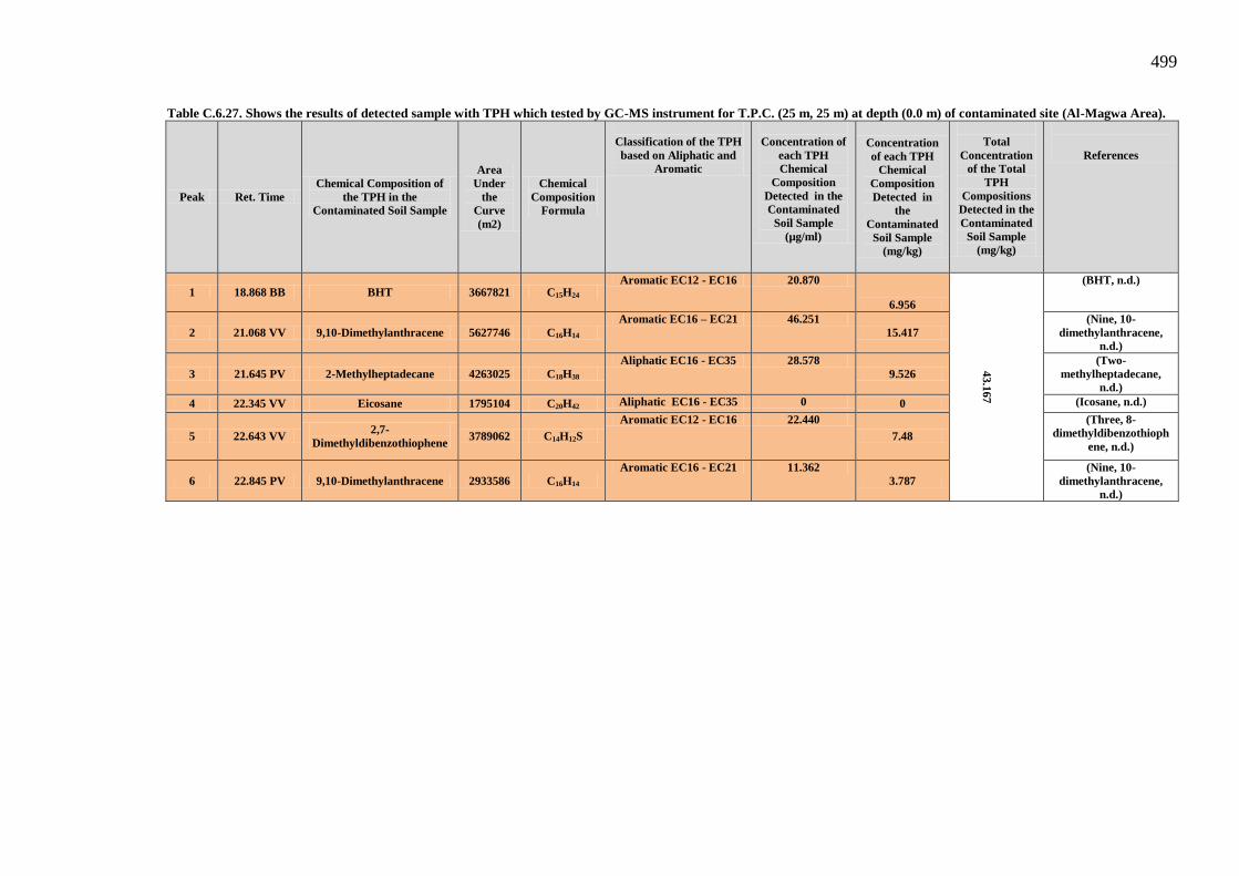
499
Table C.6.27. Shows the results of detected sample with TPH which tested by GC-MS instrument for T.P.C. (25 m, 25 m) at depth (0.0 m) of contaminated site (Al-Magwa Area).
Peak Ret. Time Chemical Composition of
the TPH in the Contaminated Soil Sample
Area Under
the Curve (m2)
Chemical Composition
Formula
Classification of the TPH based on Aliphatic and
Aromatic
Concentration of
each TPH Chemical
Composition Detected in the Contaminated
Soil Sample (µg/ml)
Concentration of each TPH
Chemical Composition Detected in
the Contaminated
Soil Sample (mg/kg)
Total
Concentration of the Total
TPH Compositions
Detected in the Contaminated
Soil Sample (mg/kg)
References
1 18.868 BB BHT 3667821 C15H24 Aromatic EC12 - EC16 20.870
6.956
43.167
(BHT, n.d.)
2 21.068 VV 9,10-Dimethylanthracene 5627746 C16H14 Aromatic EC16 – EC21 46.251
15.417 (Nine, 10-
dimethylanthracene, n.d.)
3 21.645 PV 2-Methylheptadecane 4263025 C18H38 Aliphatic EC16 - EC35 28.578
9.526 (Two-
methylheptadecane, n.d.)
4 22.345 VV Eicosane 1795104 C20H42 Aliphatic EC16 - EC35 0 0 (Icosane, n.d.)
5 22.643 VV 2,7-Dimethyldibenzothiophene
3789062 C14H12S Aromatic EC12 - EC16 22.440
7.48 (Three, 8-
dimethyldibenzothiophene, n.d.)
6 22.845 PV 9,10-Dimethylanthracene 2933586 C16H14 Aromatic EC16 - EC21 11.362
3.787 (Nine, 10-
dimethylanthracene, n.d.)

500
Figure C.6.3. The Total Ion Chromatograms (TIC) of detected soil sample with TPH for T.P.C. (25 m, 25 m) at depth (0.0 m), at
contaminated site (Al-Magwa Area).
5 . 0 0 1 0 . 0 0 1 5 . 0 0 2 0 . 0 0 2 5 . 0 0 3 0 . 0 0
5 0 0 0 0 0
1 0 0 0 0 0 0
1 5 0 0 0 0 0
2 0 0 0 0 0 0
2 5 0 0 0 0 0
3 0 0 0 0 0 0
3 5 0 0 0 0 0
4 0 0 0 0 0 0
4 5 0 0 0 0 0
5 0 0 0 0 0 0
5 5 0 0 0 0 0
6 0 0 0 0 0 0
6 5 0 0 0 0 0
7 0 0 0 0 0 0
7 5 0 0 0 0 0
8 0 0 0 0 0 0
8 5 0 0 0 0 0
T i m e - - >
A b u n d a n c e
T I C : H S 3 9 . D \ d a t a . m s
18
.8
68
21
.0
68
21
.6
45
22
.3
45
22
.6
43
22
.8
45
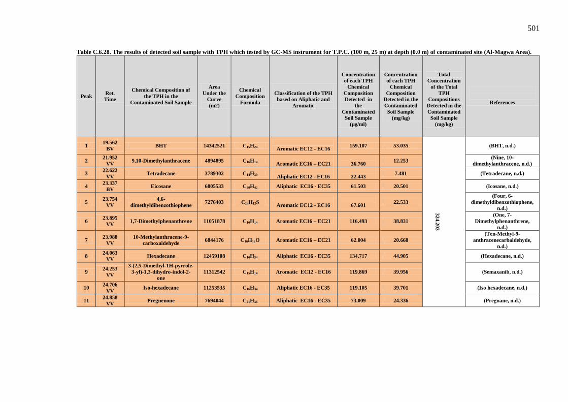
501
Table C.6.28. The results of detected soil sample with TPH which tested by GC-MS instrument for T.P.C. (100 m, 25 m) at depth (0.0 m) of contaminated site (Al-Magwa Area).
Peak Ret. Time
Chemical Composition of the TPH in the
Contaminated Soil Sample
Area Under the
Curve (m2)
Chemical Composition
Formula
Classification of the TPH based on Aliphatic and
Aromatic
Concentration of each TPH
Chemical Composition Detected in
the Contaminated
Soil Sample (µg/ml)
Concentration of each TPH
Chemical Composition
Detected in the Contaminated
Soil Sample (mg/kg)
Total
Concentration of the Total
TPH Compositions
Detected in the Contaminated
Soil Sample (mg/kg)
References
1 19.562
BV BHT 14342521 C15H24
Aromatic EC12 - EC16 159.107 53.035
324.203
(BHT, n.d.)
2 21.952
VV 9,10-Dimethylanthracene 4894895 C16H14
Aromatic EC16 – EC21
36.760 12.253 (Nine, 10-
dimethylanthracene, n.d.)
3 22.622 VV
Tetradecane 3789302 C14H30
Aliphatic EC12 - EC16
22.443 7.481 (Tetradecane, n.d.)
4 23.337
BV Eicosane 6805533 C20H42 Aliphatic EC16 - EC35 61.503 20.501 (Icosane, n.d.)
5 23.754
VV 4,6-
dimethyldibenzothiophene 7276403 C14H12S
Aromatic EC12 - EC16
67.601 22.533 (Four, 6-
dimethyldibenzothiophene, n.d.)
6 23.895
VV 1,7-Dimethylphenanthrene 11051878 C16H14 Aromatic EC16 – EC21 116.493 38.831 (One, 7-
Dimethylphenanthrene, n.d.)
7 23.988 VV
10-Methylanthracene-9-carboxaldehyde 6844176 C16H12O Aromatic EC16 – EC21 62.004 20.668
(Ten-Methyl-9-anthracenecarbaldehyde,
n.d.)
8 24.063
VV Hexadecane 12459108 C16H34 Aliphatic EC16 - EC35 134.717 44.905 (Hexadecane, n.d.)
9 24.253
VV
3-(2,5-Dimethyl-1H-pyrrole-3-yl)-1,3-dihydro-indol-2-
one 11312542 C15H14 Aromatic EC12 - EC16 119.869 39.956 (Semaxanib, n.d.)
10 24.706 VV
Iso-hexadecane 11253535 C16H34 Aliphatic EC16 - EC35 119.105 39.701 (Iso hexadecane, n.d.)
11 24.858 VV Pregnenone 7694044 C21H36 Aliphatic EC16 - EC35 73.009 24.336 (Pregnane, n.d.)
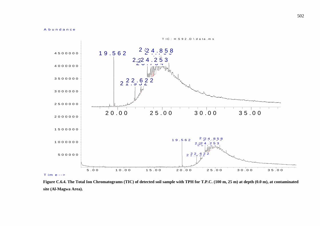
502
Figure C.6.4. The Total Ion Chromatograms (TIC) of detected soil sample with TPH for T.P.C. (100 m, 25 m) at depth (0.0 m), at contaminated
site (Al-Magwa Area).
5 . 0 0 1 0 . 0 0 1 5 . 0 0 2 0 . 0 0 2 5 . 0 0 3 0 . 0 0 3 5 . 0 0
5 0 0 0 0 0
1 0 0 0 0 0 0
1 5 0 0 0 0 0
2 0 0 0 0 0 0
2 5 0 0 0 0 0
3 0 0 0 0 0 0
3 5 0 0 0 0 0
4 0 0 0 0 0 0
4 5 0 0 0 0 0
T i m e - - >
A b u n d a n c e
T I C : H S 9 2 . D \ d a t a . m s
1 9 . 5 6 2
2 1 . 9 5 22 2 . 6 2 2
2 3 . 3 3 72 3 . 7 5 42 3 . 8 9 52 3 . 9 8 8
2 4 . 0 6 3
2 4 . 2 5 32 4 . 7 0 62 4 . 8 5 8

503
Table C.6.29. The results of detected soil sample with TPH which tested by GC-MS instrument for T.P.C. (25 m, 50 m) at depth (0.0 m) of contaminated site (Al-Magwa Area).
Peak Ret. Time Chemical Composition of
the TPH in the Contaminated Soil Sample
Area Under
the Curve (m2)
Chemical Composition
Formula
Classification of the
TPH based on Aliphatic and Aromatic
Concentration of
each TPH Chemical
Composition Detected in the Contaminated
Soil Sample (µg/ml)
Concentration of each TPH
Chemical Composition Detected in
the Contaminated
Soil Sample (mg/kg)
Total
Concentration of the Total
TPH Compositions
Detected in the Contaminated
Soil Sample (mg/kg)
References
1 3.036 BV Methyldimethoxysilane 4110314 C3H10O2Si --------
26.600
8.866
113.93
(Methyldimethoxysilane,
n.d.)
2 19.563 BV BHT 9167184 C15H24
Aromatic EC12 - EC16
92.087 30.695 (BHT, n.d.)
3 22.347 VV 1-allyl-methylindole carbaldehyde 4519003 C13H13NO
Aromatic EC12 - EC16
31.893
10.631
(One-Allyl-2-methyl-1H-indole-3-carbaldehyde,
n.d.) 4 22.456 PV Eicosane 6269607 C20H42 Aliphatic EC16 - EC35 54.563 18.187 (Icosane, n.d.)
5 22.562 VV 10-Methylanthracene-9-carboxaldehyde 3046984 C16H12O Aromatic EC16 – EC21
12.830 4.276 (Ten-Methyl-9-
anthracenecarbaldehyde, n.d.)
6 22.615 VV 1-allyl-3-methyl carbaldehyde
2624307 C13H13NO Aromatic EC12 - EC16 7.356 2.452 (One-Allyl-2-methyl-1H-indole-3-carbaldehyde,
n.d.)
7 22.896 VV 2-methyl dihydrobenzofuran
3496372 C9H10O Aromatic EC8 - EC10 18.650 18.65 (Two-Methyl-2,3-dihydro-
1-benzofuran, n.d.)
8 23.085 VV β-pregnane 3772225 C21H36 Aliphatic EC16 - EC35 22.222 7.407 (Pregnane, n.d.) 9 23.189 VV ----- 5389259 ------ ------ 43.163 14.387 --------
10 23.695 PV 4-allyl phenol 5472877 C9H10O Aromatic EC8 - EC10 44.245 14.748 (Chavicol, n.d.) 11 23.994 BV 1-octadecanol 3659348 C18H38O Aliphatic EC16 - EC35 20.760 6.92 (Octadecan-1-ol, n.d.)

504
Figure C.6.5. The Total Ion Chromatograms (TIC) of detected soil sample with TPH for T.P.C. (25 m, 50 m) at depth (0.0 m), at contaminated site
(Al-Magwa Area).
5 . 0 0 1 0 . 0 0 1 5 . 0 0 2 0 . 0 0 2 5 . 0 0 3 0 . 0 0 3 5 . 0 0
5 0 0 0 0 0
1 0 0 0 0 0 0
1 5 0 0 0 0 0
2 0 0 0 0 0 0
2 5 0 0 0 0 0
3 0 0 0 0 0 0
3 5 0 0 0 0 0
4 0 0 0 0 0 0
4 5 0 0 0 0 0
T i m e - - >
A b u n d a n c e
T I C : H S 9 6 . D \ d a t a . m s
3 . 0 3 6
1 9 . 5 6 3
2 2 . 3 4 72 2 . 4 5 62 2 . 5 6 22 2 . 6 1 5
2 2 . 8 9 62 3 . 0 8 52 3 . 1 8 9
2 3 . 6 9 52 3 . 9 9 4

505
Table C.6.30. The results of detected soil sample with TPH which tested by GC-MS instrument for T.P.C. (50 m, 50 m) at depth (0.0 m) of contaminated site (Al-Magwa Area).
Peak Ret. Time
Chemical Composition of the TPH in the
Contaminated Soil Sample
Area Under the
Curve (m2)
Chemical Composition
Formula
Classification of the
TPH based on Aliphatic and Aromatic
Concentration of each TPH
Chemical Composition
Detected in the Contaminated
Soil Sample (µg/ml)
Concentration of each TPH
Chemical Composition Detected in
the Contaminated
Soil Sample (mg/kg)
Total
Concentration of the Total
TPH Compositions
Detected in the Contaminated
Soil Sample (mg/kg)
References
1 21.128 VV 9,10-Dimethylanthracene 3628926 C16H14
Aromatic EC16 – EC21 20.366 6.788
406.83
(Nine, 10-dimethylanthracene, n.d.)
2 21.869 VV Octadecane 9887139 C18H38
Aliphatic E C16 - EC35 101.410
33.803 (Octadecane, n.d.)
3 21.953 VV 1,7-Dimethylphenanthrene 14187940 C16H14
Aromatic EC16 – EC21
157.106 52.368
(One, 7-Dimethylphenanthrene,
n.d.)
4 22.624 VV Nonadecane 15838452 C19H40 Aliphatic EC16 - EC35 178.480 59.493 (Nonadecane, n.d.)
5 23.340 VV Eicosane 26132682 C20H42 Aliphatic EC16 - EC35 311.790 103.93 (Icosane, n.d.)
6 23.758 VV Dimethylbenzothiophene 12877854 C10H10S Aromatic EC10 - EC12 140.140 46.713 (Dimethylbenzothiophene, 2016)
7 24.065 VV Heneicosane 20139838 C21H44 Aliphatic EC16 - EC35
234.183 78.061 (Heneicosane, n.d.)
8 24.856 PV ------ 14353698 ------ ------- 159.252 53.084 -------
9 25.750 VV Ethyloctadecane 8010651 C20H42 Aliphatic EC16 - EC35 77.110 25.703 (Three-Ethyloctadecane,
n.d.)

506
Figure C.6.6. The Total Ion Chromatograms (TIC) of detected soil sample with TPH for T.P.C. (50 m, 50 m) at depth (0.0 m), at contaminated site
(Al-Magwa Area).
5 . 0 0 1 0 . 0 0 1 5 . 0 0 2 0 . 0 0 2 5 . 0 0 3 0 . 0 0 3 5 . 0 0
5 0 0 0 0 0
1 0 0 0 0 0 0
1 5 0 0 0 0 0
2 0 0 0 0 0 0
2 5 0 0 0 0 0
3 0 0 0 0 0 0
3 5 0 0 0 0 0
4 0 0 0 0 0 0
4 5 0 0 0 0 0
T i m e - - >
A b u n d a n c e
T I C : H S 9 8 . D \ d a t a . m s
2 1 . 1 2 8
2 1 . 8 6 9
2 1 . 9 5 3
2 2 . 6 2 4
2 3 . 3 4 0
2 3 . 7 5 8
2 4 . 0 6 5
2 4 . 8 5 6
2 5 . 7 5 0

507
Table C.6.31. The results of detected soil sample with TPH which tested by GC-MS instrument for T.P.C. (100 m, 50 m) at depth (0.0 m) of contaminated site (Al-Magwa Area).
Peak Ret. Time
Chemical Composition of the TPH in the
Contaminated Soil Sample
Area Under the
Curve (m2)
Chemical Composition
Formula
Classification of the
TPH based on Aliphatic and Aromatic
Concentration of each TPH
Chemical Composition Detected in
the Contaminated
Soil Sample (µg/ml)
Concentration of each TPH
Chemical Composition Detected in
the Contaminated
Soil Sample (mg/kg)
Total
Concentration of the Total
TPH Compositions
Detected in the Contaminated
Soil Sample (mg/kg)
References
1 20.654 PV Tridecane 10156854 C13H28 Aliphatic EC12 - EC16 104.903 34.967
1330.087
(Tridecane, n.d.)
2 21.076 VV Heptadecane 8793615 C17H36 Aliphatic EC16 - EC35
87.249
29.083 (Heptadecane, n.d.)
3 21.129 VV 9,10-Dimethylanthracene 14433039 C16H14
Aromatic EC16 – EC21
160.280 53.42667 (Nine, 10-
dimethylanthracene, n.d.)
4 21.871 VV Octadecane 19056122 C18H38 Aliphatic EC16 - EC35 220.149 73.383 (Octadecane, n.d.)
5 21.956 VV 10-Methylanthracene-9-carboxaldehyde 42016744 C16H12O Aromatic EC16 – EC21 517.489
172.4963 (Ten-Methyl-9-
anthracenecarbaldehyde, n.d.)
6 22.579 VV Nonadecane 15866535 C19H40 Aliphatic E C16 - EC35 178.843 59.61433 (Nonadecane, n.d.)
7 22.626 VV Eicosane 28371208 C20H42 Aliphatic EC16 - EC35 340.779 113.593 (Icosane, n.d.)
8 23.153 VV β-Pregnane 18690622 C21H36 Aliphatic EC16 - EC35 215.415 71.805 (Pregnane, n.d.)
9 23.341 VV Eicosane 41694327 C20H42 Aliphatic EC16 - EC35 513.314 171.1047 (Icosane, n.d.)
10 23.700 VV ------ 30075439 ------ ------ 362.849 120.9497 ------
11 23.761 VV 2,7 Dimethylbenzothiophene 34948916 C10H10S Aromatic EC10 - EC12 425.960
141.9867 (Dimethylbenzothiophene
, n.d.)
12 23.899 VV Di-p-tolylacetylene 47199387 C16H14 Aromatic EC16 – EC21 584.604
194.868 (Di-p-Tolylacetylene,
n.d.)
13 24.067 VV n-Cetane 38843678 C16H34 Aliphatic EC16 - EC35 476.398 158.7993 (Hexadecane, n.d.)
14 24.858 VV n-Cetane 14790650 C16H34 Aliphatic EC16 - EC35 164.911 54.97033
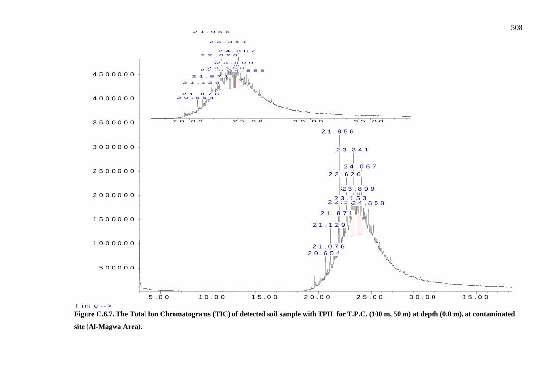
508
Figure C.6.7. The Total Ion Chromatograms (TIC) of detected soil sample with TPH for T.P.C. (100 m, 50 m) at depth (0.0 m), at contaminated
site (Al-Magwa Area).
5 . 0 0 1 0 . 0 0 1 5 . 0 0 2 0 . 0 0 2 5 . 0 0 3 0 . 0 0 3 5 . 0 0
5 0 0 0 0 0
1 0 0 0 0 0 0
1 5 0 0 0 0 0
2 0 0 0 0 0 0
2 5 0 0 0 0 0
3 0 0 0 0 0 0
3 5 0 0 0 0 0
4 0 0 0 0 0 0
4 5 0 0 0 0 0
T i m e - - >
A b u n d a n c e
T I C : H S 1 0 3 . D \ d a t a . m s
2 0 . 6 5 42 1 . 0 7 6
2 1 . 1 2 9
2 1 . 8 7 1
2 1 . 9 5 6
2 2 . 5 7 9
2 2 . 6 2 6
2 3 . 1 5 3
2 3 . 3 4 1
2 3 . 7 0 02 3 . 7 6 12 3 . 8 9 9
2 4 . 0 6 7
2 4 . 8 5 8

509
Table C.6.32. The results of detected soil sample with TPH which tested by GC-MS instrument for T.P.C. (0 m, 75 m) at depth (0.0 m) of contaminated site (Al-Magwa Area).
Peak Ret. Time Chemical Composition of
the TPH in the Contaminated Soil Sample
Area Under the
Curve (m2)
Chemical Composition Formula
Classification of the TPH based on Aliphatic and
Aromatic
Concentration of each TPH
Chemical Composition
Detected in the Contaminated
Soil Sample (µg/ml)
Concentration of each TPH
Chemical Composition Detected in
the Contaminated
Soil Sample (mg/kg)
Total
Concentration of the Total
TPH Compositions
Detected in the Contaminated
Soil Sample (mg/kg)
References
1 21.072 VV Tetramethylhexadecane 7244593 C20H42
Aliphatic EC16 - EC35 68.18 22.7
332.497
(Two, 6, 10, 14-tetramethylhexadecane,
n.d.)
2 21.650 VV Tetradecane 5395889 C14H30 Aliphatic EC12 - EC16 44.24 14.7 (Tetradecane, n.d.)
3 21.692 VV Nonadecane 4230522 C19H40 Aliphatic EC16 - EC35 30.15 10.05 (Nonadecane, n.d.)
4 21.970 VV Tri indane 6482805 C9H10
Aromatic EC8 - EC10 58.32 19.44 (Indane, n.d.)
5 22.111 VV Methylanthracene 4387001 C15H12 Aromatic EC12 - EC16 33.18 11.06 (Methylanthracene, n.d.)
6 22.344 VV Eicosane 10362137 C20H42 Aliphatic EC16 - EC35 109.561 36.52 (Icosane, n.d.)
7 22.483 VV 2,7-dimethyldibenzothiophene 9539441 C14H12S Aromatic EC12 - EC16 99.1 33.03
(Three, 8-dimethyldibenzothiophene,
n.d.)
8 22.649 VV 4,6-dimethyldibenzothiophene 11694599 C14H12S Aromatic EC12 - EC16 126.3 42.0
(Four, 6-dimethyldibenzothiophene,
n.d.)
9 22.851 VV 9,10-dimethylanthracene 10893429 C16H14 Aromatic EC16 - EC21 119.4 40.0 (Nine, 10-
dimethylanthracene, n.d.) 10 22.907 VV Substituted phenol 7032856 C7H8O Aromatic 68.447 22.815 (Two-Methylphenol, n.d.)
11 23.069 VV 2-Methylthioxanthone 10530817 C14H10OS Aromatic EC12 - EC16 109.746 36.582 (Two-Methylthioxanthone,
n.d.) 12 23.299 VV -------- 5700373 ------ ---------- 47.191 15.730 ---------
13 23.420 VV Heneicosane 9364575 C21H44 Aliphatic EC16 - EC35
98.64 33.0 (Heneicosane, n.d.)
14 23.606 PV Hexadecane 4272533 C16H34 Aliphatic EC16 - EC35 31.701 10.567 (Hexadecane, n.d.)

510
Figure C.6.8. The Total Ion Chromatograms (TIC) of detected soil sample with TPH for T.P.C. (0 m, 75 m) at depth (0.0 m), at contaminated site
(Al-Magwa Area).
5 . 0 0 1 0 . 0 0 1 5 . 0 0 2 0 . 0 0 2 5 . 0 0 3 0 . 0 0
5 0 0 0 0 0
1 0 0 0 0 0 0
1 5 0 0 0 0 0
2 0 0 0 0 0 0
2 5 0 0 0 0 0
3 0 0 0 0 0 0
3 5 0 0 0 0 0
4 0 0 0 0 0 0
4 5 0 0 0 0 0
5 0 0 0 0 0 0
5 5 0 0 0 0 0
6 0 0 0 0 0 0
T im e - - >
A b u n d a n c e
T I C : H S 2 3 . D \ d a t a . m s
21
.0
72
21
.6
50
21
.6
92
21
.9
70
22
.1
11
22
.3
44
22
.4
83
22
.6
49
22
.8
51
22
.9
07
23
.0
69
23
.2
99
23
.4
20
23
.6
06
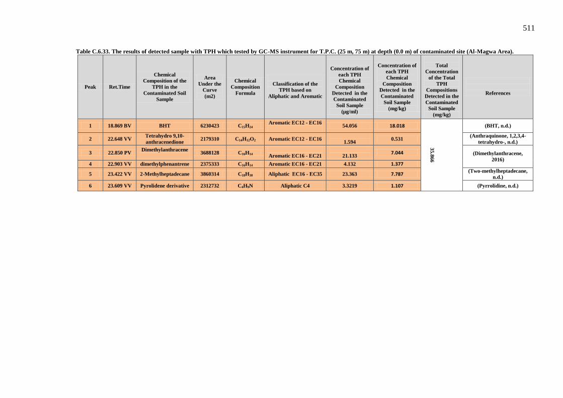
511
Table C.6.33. The results of detected sample with TPH which tested by GC-MS instrument for T.P.C. (25 m, 75 m) at depth (0.0 m) of contaminated site (Al-Magwa Area).
Peak Ret.Time
Chemical Composition of the
TPH in the Contaminated Soil
Sample
Area Under the
Curve (m2)
Chemical Composition
Formula
Classification of the
TPH based on Aliphatic and Aromatic
Concentration of
each TPH Chemical
Composition Detected in the Contaminated
Soil Sample (µg/ml)
Concentration of each TPH Chemical
Composition Detected in the Contaminated
Soil Sample (mg/kg)
Total
Concentration of the Total
TPH Compositions
Detected in the Contaminated
Soil Sample (mg/kg)
References
1 18.869 BV BHT 6230423 C15H24 Aromatic EC12 - EC16
54.056 18.018
35.866
(BHT, n.d.)
2 22.648 VV Tetrahydro 9,10-anthracenedione 2179310 C14H12O2 Aromatic EC12 - EC16
1.594 0.531
(Anthraquinone, 1,2,3,4-tetrahydro-, n.d.)
3 22.850 PV Dimethylanthracene 3688128 C16H14
Aromatic EC16 - EC21
21.133
7.044 (Dimethylanthracene, 2016)
4 22.903 VV dimethylphenantrene 2375333 C16H14 Aromatic EC16 - EC21 4.132 1.377
5 23.422 VV 2-Methylheptadecane 3860314 C18H38 Aliphatic EC16 - EC35 23.363 7.787 (Two-methylheptadecane,
n.d.)
6 23.609 VV Pyrolidene derivative 2312732 C4H9N Aliphatic C4 3.3219 1.107 (Pyrrolidine, n.d.)
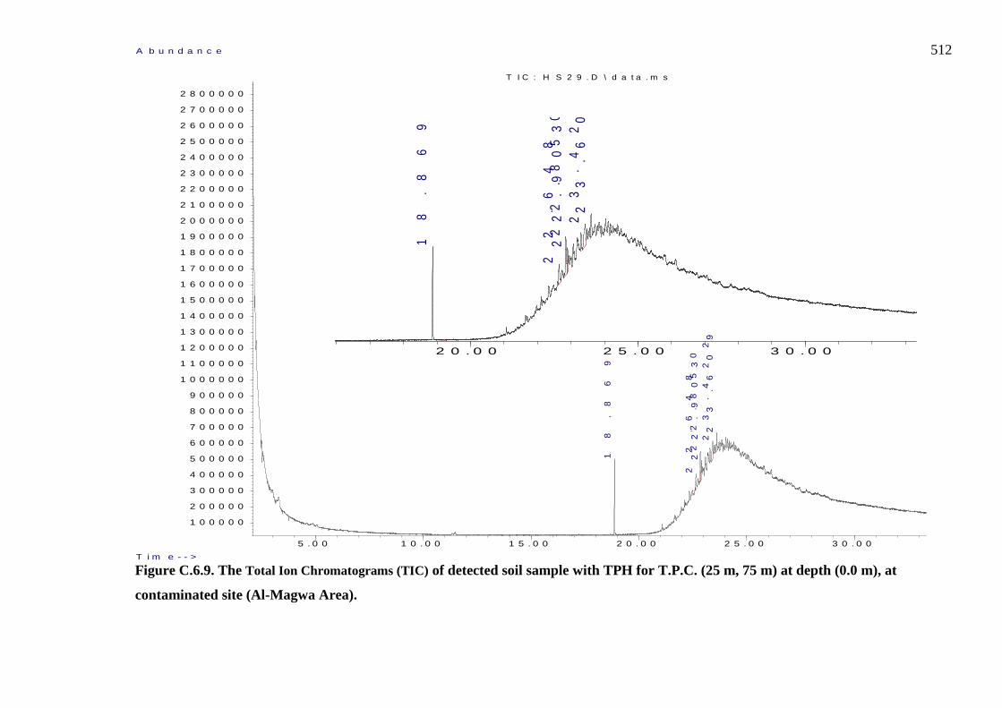
512
Figure C.6.9. The Total Ion Chromatograms (TIC) of detected soil sample with TPH for T.P.C. (25 m, 75 m) at depth (0.0 m), at
contaminated site (Al-Magwa Area).
5 . 0 0 1 0 . 0 0 1 5 . 0 0 2 0 . 0 0 2 5 . 0 0 3 0 . 0 0
1 0 0 0 0 0
2 0 0 0 0 0
3 0 0 0 0 0
4 0 0 0 0 0
5 0 0 0 0 0
6 0 0 0 0 0
7 0 0 0 0 0
8 0 0 0 0 0
9 0 0 0 0 0
1 0 0 0 0 0 0
1 1 0 0 0 0 0
1 2 0 0 0 0 0
1 3 0 0 0 0 0
1 4 0 0 0 0 0
1 5 0 0 0 0 0
1 6 0 0 0 0 0
1 7 0 0 0 0 0
1 8 0 0 0 0 0
1 9 0 0 0 0 0
2 0 0 0 0 0 0
2 1 0 0 0 0 0
2 2 0 0 0 0 0
2 3 0 0 0 0 0
2 4 0 0 0 0 0
2 5 0 0 0 0 0
2 6 0 0 0 0 0
2 7 0 0 0 0 0
2 8 0 0 0 0 0
T i m e - - >
A b u n d a n c e
T I C : H S 2 9 . D \ d a t a . m s
18
.8
69
22
.6
48
22
.8
50
22
.9
03
23
.4
22
23
.6
09

513
Table C.6.34. The results of detected soil sample with TPH which tested by GC-MS instrument for T.P.C. (50 m, 75 m) at depth (0.0 m) of contaminated site (Al-Magwa Area).
Peak Ret. Time
Chemical Composition of the TPH in the
Contaminated Soil Sample
Area Under the
Curve (m2)
Chemical Composition
Formula
Classification of the
TPH based on Aliphatic and Aromatic
Concentration of each TPH
Chemical Composition
Detected in the Contaminated
Soil Sample (µg/ml)
Concentration of each TPH
Chemical Composition Detected in
the Contaminated
Soil Sample (mg/kg)
Total
Concentration of the Total
TPH Compositions
Detected in the Contaminated
Soil Sample (mg/kg)
References
1 3.028 BV Methyldimethoxysilane 6453289 C3H10O2Si -------- 56.942 18.980
865.223
(Methyldimethoxysilane, n.d.)
2 21.869 BV Octadecane 10700879 C18H38 Aliphatic EC16 - EC35
111.948
37.316 (Octadecane, n.d.)
3 21.953 VV Di-p-tolylacetylene 21365693 C16H14
Aromatic EC16 – EC21 250.058
83.352 (Di-p-Tolylacetylene, n.d.)
4 22.577 VV Eicosane 8918550 C20H42 Aliphatic EC16 - EC35 88.867 29.622 (Icosane, n.d.)
5 22.625 VV Nonadecane 25281416 C19H40 Aliphatic EC16 - EC35 300.766
100.255 (Nonadecane, n.d.)
6 22.995 VV 10-Methylanthracene-9-carboxaldehyde
16162900 C16H12O Aromatic EC16 – EC21 182.681 60.893 (Ten-Methyl-9-
anthracenecarbaldehyde, n.d.)
7 23.151 VV 1-Methylphenanthrene 12251310 C15H12 Aromatic EC12 - EC16 132.026 44.008 (Methylphenanthrene, n.d.)
8 23.340 VV Eicosane 31256101 C20H42 Aliphatic EC16 - EC35 378.138 126.046 (Icosane, n.d.)
9 23.398 VV 2,7-Dimethylbenzothiophene
17564077 C10H10S Aromatic EC10 - EC12 200.827 66.942 (Dimethylbenzothiophene,
2016)
10 23.760 VV Di-p-tolylacetylene 21851494 C16H14 Aromatic EC16 – EC21 256.349 85.449 (Di-p-Tolylacetylene, n.d.)
11 23.896 VV 2-Methylheptadecane 25899580 C18H38 Aliphatic EC16 - EC35 308.771 102.923 (Two-methylheptadecane, n.d.)
12 24.065 VV n-Heneicosane 20970757 C21H44 Aliphatic EC16 - EC35 244.943 81.647 (Heneicosane, n.d.)
13 24.855 PV Docosane 12891156 C22H46 Aliphatic EC16 - EC35 140.312 46.770 (Docosane, n.d.)
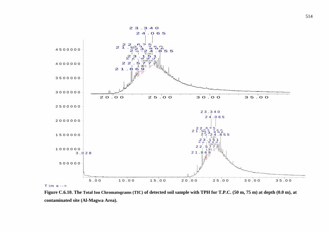
514
Figure C.6.10. The Total Ion Chromatograms (TIC) of detected soil sample with TPH for T.P.C. (50 m, 75 m) at depth (0.0 m), at
contaminated site (Al-Magwa Area).
5 . 0 0 1 0 . 0 0 1 5 . 0 0 2 0 . 0 0 2 5 . 0 0 3 0 . 0 0 3 5 . 0 0
5 0 0 0 0 0
1 0 0 0 0 0 0
1 5 0 0 0 0 0
2 0 0 0 0 0 0
2 5 0 0 0 0 0
3 0 0 0 0 0 0
3 5 0 0 0 0 0
4 0 0 0 0 0 0
4 5 0 0 0 0 0
T i m e - - >
A b u n d a n c e
T I C : H S 1 0 1 . D \ d a t a . m s
3 . 0 2 8 2 1 . 8 6 9
2 1 . 9 5 3
2 2 . 5 7 7
2 2 . 6 2 5
2 2 . 9 9 52 3 . 1 5 1
2 3 . 3 4 0
2 3 . 3 9 82 3 . 7 6 02 3 . 8 9 6
2 4 . 0 6 5
2 4 . 8 5 5

515
Table C.6.35. The results of detected soil sample with TPH which tested by GC-MS instrument for T.P.C. (75 m, 75 m) at depth (0.0 m) of contaminated site (Al-Magwa Area).
Peak Ret. Time Chemical Composition of
the TPH in the Contaminated Soil Sample
Area Under the
Curve (m2)
Chemical Composition
Formula
Classification of the
TPH based on Aliphatic and Aromatic
Concentration of each TPH
Chemical Composition Detected in
the Contaminated
Soil Sample (µg/ml)
Concentration of each TPH
Chemical Composition Detected in
the Contaminated
Soil Sample (mg/kg)
Total
Concentration of the Total
TPH Compositions
Detected in the
Contaminated Soil Sample
(mg/kg)
References
1 3.012 BV Methyldimethoxysilane 7292440 C3H10O2Si -------- 67.809 22.603
567.336
(Methyldimethoxysilane,
n.d.)
2 21.953 VV 9,10-Dimethylanthracene 13623920 C16H14 Aromatic EC16 – EC21
149.801
49.933 (Nine, 10-
dimethylanthracene, n.d.)
3 22.577 VV Heneicosane 12600015 C21H44 Aliphatic EC16- EC35 136.542
45.514 (Heneicosane, n.d.)
4 22.625 VV Nonadecane 18699504 C19H40 Aliphatic EC16 - EC35
215.530 71.843 (Nonadecane, n.d.)
5 23.339 VV Eicosane 9001903 C20H42 Aliphatic EC16 - EC35 89.947 29.982 (Icosane, n.d.)
6 23.397 VV 2,7-
Dimethyldibenzothiophene 17362242 C14H12S Aromatic EC12 - EC16 198.213 66.071 (Three, 8-
dimethyldibenzothiophene, n.d.)
7 23.562 VV 1,7-
Dimethyldibenzothiophene 14249069 C14H12S Aromatic EC12 - EC16 157.897 52.632 (One, 7-
Dimethyldibenzothiophene, n.d.)
8 23.697 VV Di-p-tolylacetylene 11635172 C16H14 Aromatic EC16 – EC21
124.047 41.349
(Di-p-Tolylacetylene, n.d.)
9 23.759 VV ------- 13006757 ------- ------- 141.809 47.269 ----------- 10 23.895 VV Pentadecane 11052537 C15H32 Aliphatic EC12 - EC16 116.502 38.834 (Pentadecane, n.d.)
11 23.991 VV 1,7-Dimethylphenanthrene 18253314 C16H14 Aromatic EC16 - EC21 209.752 69.917 (One, 7-
Dimethylphenanthrene, n.d.)
12 24.065 VV Cetane 10216906 C16H34 Aliphatic EC16 - EC35 105.681 35.227 (Hexadecane, n.d.) 13 24.706 VV β-Pregnane 14583468 C21H36 Aliphatic EC16 - EC35 162.228 54.076 (Pregnane, 2016) 14 24.856 PV Docosane 4204300 C22H46 Aliphatic EC16 - EC35 27.817 9.272 (Docosane, n.d.) 15 25.750 PV Pregenone 2678578 C21H36 Aliphatic EC16 - EC35 8.0596 2.686 (Pregnane, 2016)

516
Figure C.6.11. The Total Ion Chromatograms (TIC) of detected soil sample with TPH for T.P.C. (75 m, 75 m) at depth (0.0 m), at contaminated
site (Al-Magwa Area).
5 . 0 0 1 0 . 0 0 1 5 . 0 0 2 0 . 0 0 2 5 . 0 0 3 0 . 0 0 3 5 . 0 0
5 0 0 0 0 0
1 0 0 0 0 0 0
1 5 0 0 0 0 0
2 0 0 0 0 0 0
2 5 0 0 0 0 0
3 0 0 0 0 0 0
3 5 0 0 0 0 0
4 0 0 0 0 0 0
4 5 0 0 0 0 0
T i m e - - >
A b u n d a n c e
T I C : H S 1 0 0 . D \ d a t a . m s
3 . 0 1 2
2 1 . 9 5 3
2 2 . 5 7 7
2 2 . 6 2 5
2 3 . 3 3 9
2 3 . 3 9 72 3 . 5 6 22 3 . 6 9 72 3 . 7 5 92 3 . 8 9 52 3 . 9 9 1
2 4 . 0 6 5
2 4 . 7 0 6
2 4 . 8 5 6
2 5 . 7 5 0
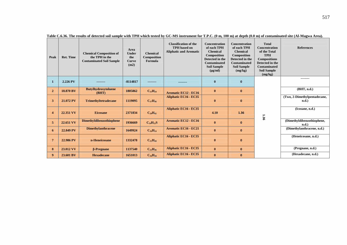
517
Table C.6.36. The results of detected soil sample with TPH which tested by GC-MS instrument for T.P.C. (0 m, 100 m) at depth (0.0 m) of contaminated site (Al-Magwa Area).
Peak Ret. Time Chemical Composition of
the TPH in the Contaminated Soil Sample
Area Under
the Curve (m2)
Chemical Composition
Formula
Classification of the
TPH based on Aliphatic and Aromatic
Concentration of each TPH
Chemical Composition
Detected in the Contaminated
Soil Sample (µg/ml)
Concentration of each TPH
Chemical Composition
Detected in the Contaminated
Soil Sample (mg/kg)
Total
Concentration of the Total
TPH Compositions
Detected in the Contaminated
Soil Sample (mg/kg)
References
1 2.226 PV -------- -8114817 --------
-------- 0 0
1.3
6
--------
2 18.870 BV Butylhydroxytoluene (BHT) 1805862 C15H24
Aromatic EC12 - EC16 0 0
(BHT, n.d.)
3 21.072 PV Trimethyltetradecane 1119095 C17H36 Aliphatic EC16 - EC35
0 0 (Two, 2-Dimethylpentadecane,
n.d.)
4 22.351 VV Eicosane 2371834 C20H42 Aliphatic EC16 - EC35
4.10 1.36 (Icosane, n.d.)
5 22.651 VV Dimethyldibenzothiophene 1936669 C14H12S Aromatic EC12 - EC16 0 0
(Dimethyldibenzothiophene, n.d.)
6 22.849 PV Dimethylanthracene
1649924 C16H14 Aromatic EC16 - EC21
0 0 (Dimethylanthracene, n.d.)
7 22.986 PV n-Heneicosane 1332478 C21H44 Aliphatic EC16 - EC35
0 0 (Heneicosane, n.d.)
8 23.012 VV β-Pregnane 1137540 C21H36 Aliphatic EC16 - EC35 0 0 (Pregnane, n.d.)
9 23.601 BV Hexadecane 1651013 C16H34 Aliphatic EC16 - EC35 0 0 (Hexadecane, n.d.)

518
Figure C.6.12. The Total Ion Chromatograms (TIC) of detected soil sample with TPH for T.P.C. (0 m, 100 m) at depth (0.0 m), at contaminated
site (Al-Magwa Area).
5 . 0 0 1 0 . 0 0 1 5 . 0 0 2 0 . 0 0 2 5 . 0 0 3 0 . 0 0
1 0 0 0 0 0
2 0 0 0 0 0
3 0 0 0 0 0
4 0 0 0 0 0
5 0 0 0 0 0
6 0 0 0 0 0
7 0 0 0 0 0
8 0 0 0 0 0
9 0 0 0 0 0
1 0 0 0 0 0 0
1 1 0 0 0 0 0
1 2 0 0 0 0 0
1 3 0 0 0 0 0
1 4 0 0 0 0 0
1 5 0 0 0 0 0
1 6 0 0 0 0 0
1 7 0 0 0 0 0
1 8 0 0 0 0 0
1 9 0 0 0 0 0
2 0 0 0 0 0 0
2 1 0 0 0 0 0
2 2 0 0 0 0 0
2 3 0 0 0 0 0
2 4 0 0 0 0 0
2 5 0 0 0 0 0
2 6 0 0 0 0 0
2 7 0 0 0 0 0
2 8 0 0 0 0 0
2 9 0 0 0 0 0
3 0 0 0 0 0 0
3 1 0 0 0 0 0
3 2 0 0 0 0 0
3 3 0 0 0 0 0
T i m e - - >
A b u n d a n c e
T I C : H S 1 8 . D \ d a t a . m s
2 . 2 2 6
1 8 . 8 7 02 1 . 0 7 2
2 2 . 3 5 12 2 . 6 5 12 2 . 8 4 92 2 . 9 8 62 3 . 0 1 22 3 . 6 0 1
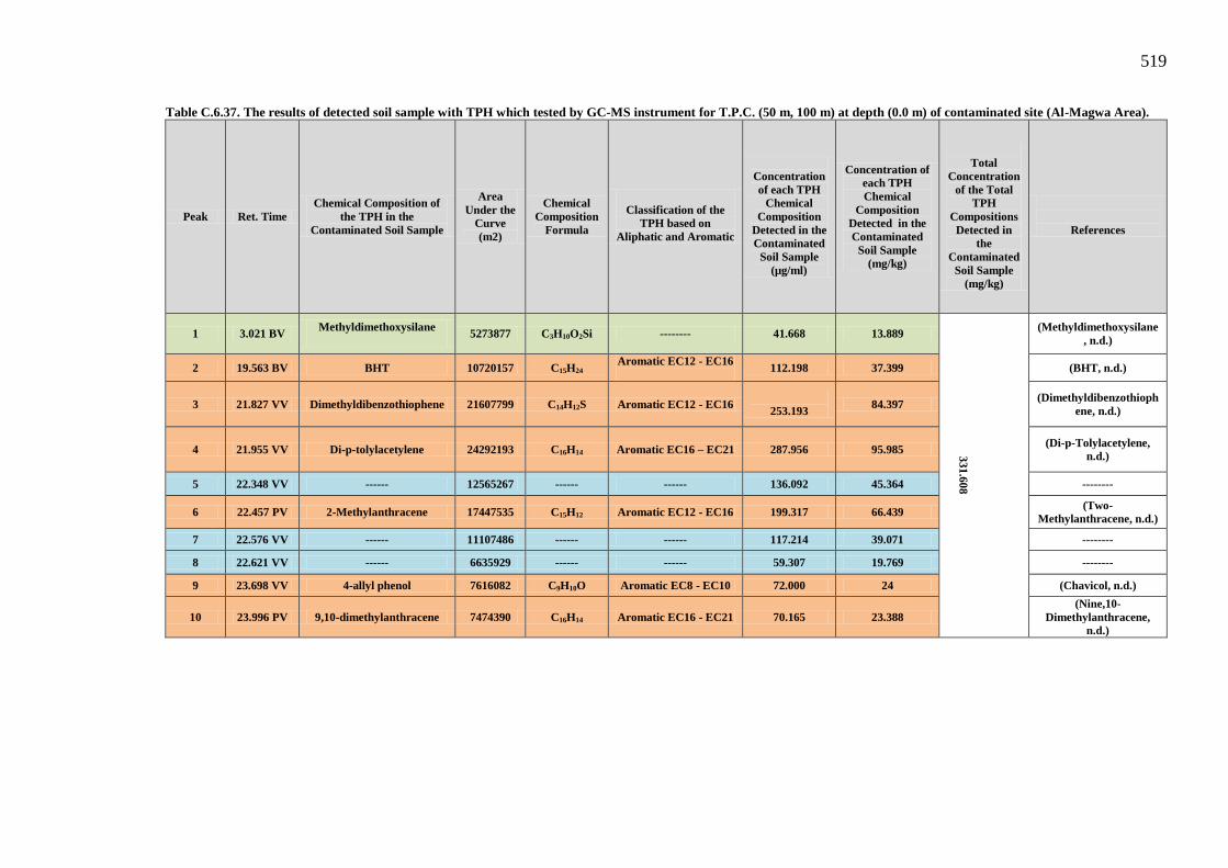
519
Table C.6.37. The results of detected soil sample with TPH which tested by GC-MS instrument for T.P.C. (50 m, 100 m) at depth (0.0 m) of contaminated site (Al-Magwa Area).
Peak Ret. Time Chemical Composition of
the TPH in the Contaminated Soil Sample
Area Under the
Curve (m2)
Chemical Composition
Formula
Classification of the
TPH based on Aliphatic and Aromatic
Concentration of each TPH
Chemical Composition
Detected in the Contaminated
Soil Sample (µg/ml)
Concentration of each TPH Chemical
Composition Detected in the Contaminated
Soil Sample (mg/kg)
Total
Concentration of the Total
TPH Compositions
Detected in the
Contaminated Soil Sample
(mg/kg)
References
1 3.021 BV Methyldimethoxysilane
5273877 C3H10O2Si -------- 41.668 13.889
331.608
(Methyldimethoxysilane, n.d.)
2 19.563 BV BHT 10720157 C15H24 Aromatic EC12 - EC16
112.198 37.399 (BHT, n.d.)
3 21.827 VV Dimethyldibenzothiophene 21607799 C14H12S Aromatic EC12 - EC16
253.193 84.397 (Dimethyldibenzothioph
ene, n.d.)
4 21.955 VV Di-p-tolylacetylene 24292193 C16H14 Aromatic EC16 – EC21 287.956 95.985 (Di-p-Tolylacetylene, n.d.)
5 22.348 VV ------ 12565267 ------ ------ 136.092 45.364 --------
6 22.457 PV 2-Methylanthracene 17447535 C15H12 Aromatic EC12 - EC16 199.317 66.439 (Two-Methylanthracene, n.d.)
7 22.576 VV ------ 11107486 ------ ------ 117.214 39.071 --------
8 22.621 VV ------ 6635929 ------ ------ 59.307 19.769 --------
9 23.698 VV 4-allyl phenol 7616082 C9H10O Aromatic EC8 - EC10 72.000 24 (Chavicol, n.d.)
10 23.996 PV 9,10-dimethylanthracene 7474390 C16H14 Aromatic EC16 - EC21 70.165 23.388 (Nine,10-
Dimethylanthracene, n.d.)

520
Figure C.6.13. The Total Ion Chromatograms (TIC) of detected soil sample with TPH for T.P.C. (50 m, 100 m) at depth (0.0 m), at contaminated
site (Al-Magwa Area).
5 . 0 0 1 0 . 0 0 1 5 . 0 0 2 0 . 0 0 2 5 . 0 0 3 0 . 0 0 3 5 . 0 0
5 0 0 0 0 0
1 0 0 0 0 0 0
1 5 0 0 0 0 0
2 0 0 0 0 0 0
2 5 0 0 0 0 0
3 0 0 0 0 0 0
3 5 0 0 0 0 0
4 0 0 0 0 0 0
4 5 0 0 0 0 0
T i m e - - >
A b u n d a n c e
T I C : H S 1 0 4 . D \ d a t a . m s
3 . 0 2 11 9 . 5 6 3
2 1 . 8 2 7
2 1 . 9 5 5
2 2 . 3 4 8
2 2 . 4 5 72 2 . 5 7 62 2 . 6 2 1
2 3 . 6 9 82 3 . 9 9 6
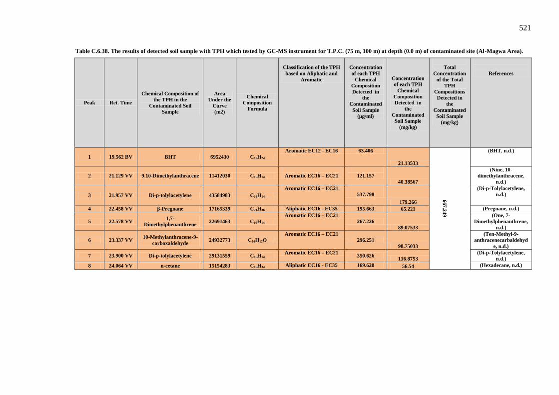
521
Table C.6.38. The results of detected soil sample with TPH which tested by GC-MS instrument for T.P.C. (75 m, 100 m) at depth (0.0 m) of contaminated site (Al-Magwa Area).
Peak Ret. Time
Chemical Composition of the TPH in the
Contaminated Soil Sample
Area Under the
Curve (m2)
Chemical Composition
Formula
Classification of the TPH based on Aliphatic and
Aromatic
Concentration of each TPH
Chemical Composition Detected in
the Contaminated
Soil Sample (µg/ml)
Concentration of each TPH
Chemical Composition Detected in
the Contaminated
Soil Sample (mg/kg)
Total
Concentration of the Total
TPH Compositions
Detected in the
Contaminated Soil Sample
(mg/kg)
References
1 19.562 BV BHT 6952430 C15H24 Aromatic EC12 - EC16 63.406
21.13533
667.249
(BHT, n.d.)
2 21.129 VV 9,10-Dimethylanthracene 11412030 C16H14
Aromatic EC16 – EC21
121.157 40.38567
(Nine, 10-dimethylanthracene,
n.d.)
3 21.957 VV Di-p-tolylacetylene 43584983 C16H14 Aromatic EC16 – EC21
537.798
179.266
(Di-p-Tolylacetylene, n.d.)
4 22.458 VV β-Pregnane 17165339 C21H36 Aliphatic EC16 - EC35 195.663 65.221 (Pregnane, n.d.)
5 22.578 VV 1,7-Dimethylphenanthrene 22691463 C16H14
Aromatic EC16 – EC21 267.226
89.07533
(One, 7-Dimethylphenanthrene,
n.d.)
6 23.337 VV 10-Methylanthracene-9-carboxaldehyde
24932773 C16H12O Aromatic EC16 – EC21
296.251 98.75033
(Ten-Methyl-9-anthracenecarbaldehyd
e, n.d.)
7 23.900 VV Di-p-tolylacetylene 29131559 C16H14 Aromatic EC16 – EC21 350.626 116.8753
(Di-p-Tolylacetylene, n.d.)
8 24.064 VV n-cetane 15154283 C16H34 Aliphatic EC16 - EC35 169.620 56.54 (Hexadecane, n.d.)
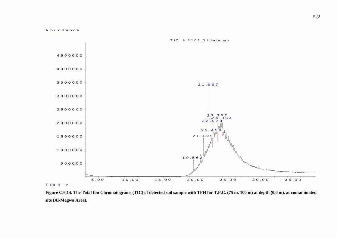
522
Figure C.6.14. The Total Ion Chromatograms (TIC) of detected soil sample with TPH for T.P.C. (75 m, 100 m) at depth (0.0 m), at contaminated
site (Al-Magwa Area).
5 . 0 0 1 0 . 0 0 1 5 . 0 0 2 0 . 0 0 2 5 . 0 0 3 0 . 0 0 3 5 . 0 0
5 0 0 0 0 0
1 0 0 0 0 0 0
1 5 0 0 0 0 0
2 0 0 0 0 0 0
2 5 0 0 0 0 0
3 0 0 0 0 0 0
3 5 0 0 0 0 0
4 0 0 0 0 0 0
4 5 0 0 0 0 0
T i m e - - >
A b u n d a n c e
T I C : H S 1 0 6 . D \ d a t a . m s
1 9 . 5 6 2
2 1 . 1 2 9
2 1 . 9 5 7
2 2 . 4 5 8
2 2 . 5 7 8
2 3 . 3 3 72 3 . 9 0 02 4 . 0 6 4
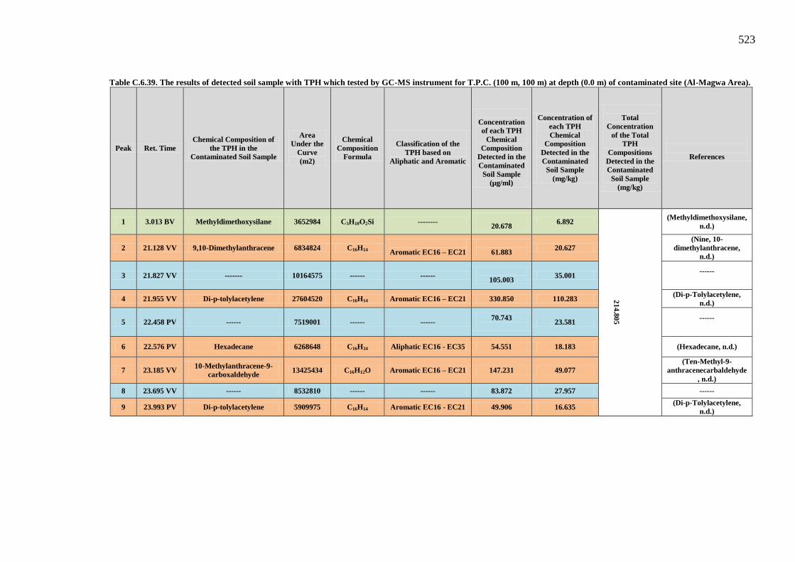
523
Table C.6.39. The results of detected soil sample with TPH which tested by GC-MS instrument for T.P.C. (100 m, 100 m) at depth (0.0 m) of contaminated site (Al-Magwa Area).
Peak Ret. Time Chemical Composition of
the TPH in the Contaminated Soil Sample
Area Under the
Curve (m2)
Chemical Composition
Formula
Classification of the
TPH based on Aliphatic and Aromatic
Concentration of each TPH
Chemical Composition
Detected in the Contaminated
Soil Sample (µg/ml)
Concentration of each TPH Chemical
Composition Detected in the Contaminated
Soil Sample (mg/kg)
Total
Concentration of the Total
TPH Compositions
Detected in the Contaminated
Soil Sample (mg/kg)
References
1 3.013 BV Methyldimethoxysilane 3652984 C3H10O2Si -------- 20.678
6.892
214.805
(Methyldimethoxysilane, n.d.)
2 21.128 VV 9,10-Dimethylanthracene 6834824 C16H14
Aromatic EC16 – EC21
61.883 20.627 (Nine, 10-
dimethylanthracene, n.d.)
3 21.827 VV ------- 10164575 ------ ------
105.003 35.001 ------
4 21.955 VV Di-p-tolylacetylene 27604520 C16H14 Aromatic EC16 – EC21 330.850 110.283 (Di-p-Tolylacetylene, n.d.)
5 22.458 PV ------ 7519001 ------ ------ 70.743
23.581 ------
6 22.576 PV Hexadecane 6268648 C16H34 Aliphatic EC16 - EC35 54.551 18.183 (Hexadecane, n.d.)
7 23.185 VV 10-Methylanthracene-9-carboxaldehyde 13425434 C16H12O Aromatic EC16 – EC21 147.231 49.077
(Ten-Methyl-9-anthracenecarbaldehyde
, n.d.)
8 23.695 VV ------ 8532810 ------ ------ 83.872 27.957 ------
9 23.993 PV Di-p-tolylacetylene 5909975 C16H14 Aromatic EC16 - EC21 49.906 16.635 (Di-p-Tolylacetylene, n.d.)

524
Figure C.6.15. The Total Ion Chromatograms (TIC) of detected soil sample with TPH for T.P.C. (100 m, 100 m) at depth (0.0 m), at
contaminated site (Al-Magwa Area).
5 . 0 0 1 0 . 0 0 1 5 . 0 0 2 0 . 0 0 2 5 . 0 0 3 0 . 0 0 3 5 . 0 0
5 0 0 0 0 0
1 0 0 0 0 0 0
1 5 0 0 0 0 0
2 0 0 0 0 0 0
2 5 0 0 0 0 0
3 0 0 0 0 0 0
3 5 0 0 0 0 0
4 0 0 0 0 0 0
4 5 0 0 0 0 0
T i m e - - >
A b u n d a n c e
T I C : H S 1 0 2 . D \ d a t a . m s
3 . 0 1 3 2 1 . 1 2 82 1 . 8 2 7
2 1 . 9 5 5
2 2 . 4 5 8
2 2 . 5 7 62 3 . 1 8 52 3 . 6 9 52 3 . 9 9 3

525
At depth (0.25 m) at contaminated site

526
Table C.6.40. The results of detected soil sample with TPH which tested by GC-MS instrument for T.P.C. (100 m, 0 m) at depth (0.25 m) of contaminated site (Al-Magwa Area).
Peak Ret. Time
Chemical Composition of the TPH in the Contaminated
Soil Sample
Area Under the
Curve (m2)
Chemical Composition
Formula
Classification of the
TPH based on Aliphatic and Aromatic
Concentration of
each TPH Chemical
Composition Detected in the Contaminated
Soil Sample (µg/ml)
Concentration of each TPH Chemical
Composition Detected in the
Contaminated Soil Sample (mg/kg)
Total Concentration of
the Total TPH Compositions Detected
in the Contaminated Soil Sample (mg/kg)
References
1 18.867 BB BHT 2642984 C15H24 Aromatic EC12 - EC16 7.598 2.532 2.532 (BHT, n.d.)

527
Figure C.6.16. The Total Ion Chromatograms (TIC) of detected soil sample for T.P.C. (100 m, 0 m) at depth (0.25 m), at contaminated site (Al-
Magwa Area).
5 .00 10 .00 15 .00 20 .00 25 .00 30 .00
500000
1000000
1500000
2000000
2500000
3000000
3500000
4000000
4500000
5000000
5500000
6000000
6500000
7000000
7500000
T im e - ->
A bundanc e
T IC : H S 3 6 .D \ d a ta .m s
18
.8
67
5 .00 10 .00 15 .00 20 .00 25 .00 30 .00
500000
1000000
1500000
2000000
2500000
3000000
3500000
4000000
4500000
5000000
5500000
6000000
6500000
7000000
7500000
T im e - ->
A bundanc e
T IC : H S 3 6 .D \ d a ta .m s
18
.86
7

528
Table C.6.41. The results of detected soil sample with TPH which tested by GC-MS instrument for T.P.C. (0 m, 25 m) at depth (0.25 m) of contaminated site (Al-Magwa Area).
Peak Ret. Time Chemical Composition of the
TPH in the Contaminated Soil Sample
Area Under
the Curve (m2)
Chemical Composition
Formula
Classification of the
TPH based on Aliphatic and Aromatic
Concentration of each TPH
Chemical Composition Detected in
the Contaminated
Soil Sample (µg/ml)
Concentration of each TPH
Chemical Composition Detected in
the Contaminated
Soil Sample (mg/kg)
Total
Concentration of the Total
TPH Compositions
Detected in the
Contaminated Soil Sample
(mg/kg)
References
1 20.262 VV Heptadecane 3083330 C17H36 Aliphatic EC16 - EC35 13.30 4.433
42.3
(Heptadecane, n.d.)
2 20.993 PV Octadecane 1801359 C18H38 Aliphatic EC16 - EC35 0 0 (Octadecane, n.d.)
3 21.689 VV Hexadecane 3026865 C16H34 Aliphatic EC16 - EC35 12.569 4.189 (Hexadecane, n.d.)
4 22.346 PV pentadecane 4112831 C15H32 Aliphatic EC12 - EC16 26.633 8.877 (Pentadecane, n.d.)
5 22.644 VV 4,6-Dimethyldibenzothiophene 4652408 C14H12S Aromatic EC12 - EC16 33.620 11.206 (Four, 6-
dimethyldibenzothiophene, n.d.)
6 22.848 VV 9,10-Dimethylanthracene 3941521 C16H14 Aromatic EC16 - EC21 24.414 8.138 (Nine, 10-
dimethylanthracene, n.d.)
7 23.598 PV 10-Methylanthracene-9-carboxaldehyde 3320329 C16H12O Aromatic EC16 - EC21 16.370 5.456
(Ten-Methyl-9-anthracenecarbaldehyde,
n.d.)

529
Figure C.6.17. The Total Ion Chromatograms (TIC) of detected soil sample for T.P.C. (0 m, 25 m) at depth (0.25 m), at contaminated site (Al-
Magwa Area).
5.00 10.00 15.00 20.00 25.00 30.00
200000
400000
600000
800000
1000000
1200000
1400000
1600000
1800000
2000000
2200000
2400000
2600000
2800000
3000000
3200000
3400000
3600000
T im e-->
Abundanc e
T IC : H S 5 7 .D \ d a ta .m s
20
.2
62
20
.9
93
21
.6
89
22
.3
46
22
.6
44
22
.8
48
23
.5
98
5.00 10.00 15.00 20.00 25.00 30.00
200000
400000
600000
800000
1000000
1200000
1400000
1600000
1800000
2000000
2200000
2400000
2600000
2800000
3000000
3200000
3400000
3600000
T im e-->
Abundanc e
T IC : H S 5 7 .D \ d a ta .m s
20
.26
22
0.9
93
21
.68
92
2.3
46
22
.64
42
2.8
48
23
.59
8
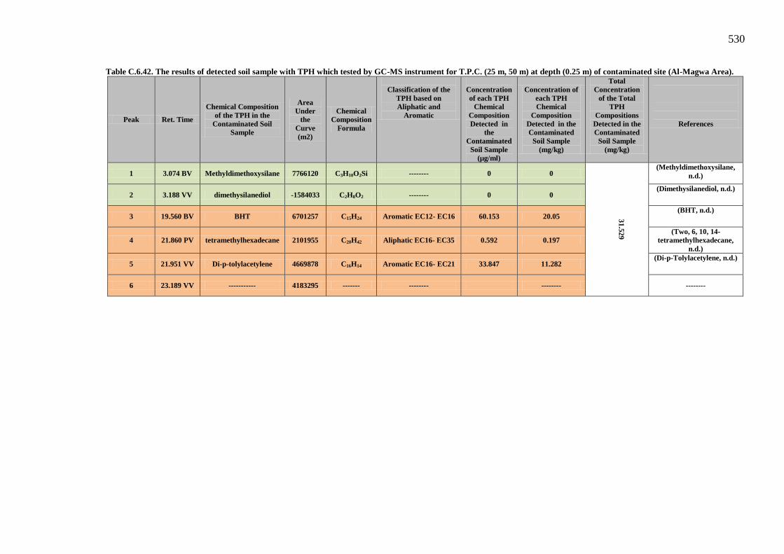
530
Table C.6.42. The results of detected soil sample with TPH which tested by GC-MS instrument for T.P.C. (25 m, 50 m) at depth (0.25 m) of contaminated site (Al-Magwa Area).
Peak Ret. Time
Chemical Composition of the TPH in the
Contaminated Soil Sample
Area Under
the Curve (m2)
Chemical Composition
Formula
Classification of the
TPH based on Aliphatic and
Aromatic
Concentration of each TPH
Chemical Composition Detected in
the Contaminated
Soil Sample (µg/ml)
Concentration of each TPH Chemical
Composition Detected in the Contaminated
Soil Sample (mg/kg)
Total Concentration
of the Total TPH
Compositions Detected in the Contaminated
Soil Sample (mg/kg)
References
1 3.074 BV Methyldimethoxysilane 7766120 C3H10O2Si -------- 0 0
31.529
(Methyldimethoxysilane, n.d.)
2 3.188 VV dimethysilanediol -1584033 C2H8O2 -------- 0 0 (Dimethysilanediol, n.d.)
3 19.560 BV BHT 6701257 C15H24 Aromatic EC12- EC16 60.153 20.05 (BHT, n.d.)
4 21.860 PV tetramethylhexadecane 2101955 C20H42 Aliphatic EC16- EC35 0.592 0.197 (Two, 6, 10, 14-
tetramethylhexadecane, n.d.)
5 21.951 VV Di-p-tolylacetylene 4669878 C16H14 Aromatic EC16- EC21 33.847 11.282 (Di-p-Tolylacetylene, n.d.)
6 23.189 VV ----------- 4183295 ------- -------- -------- --------
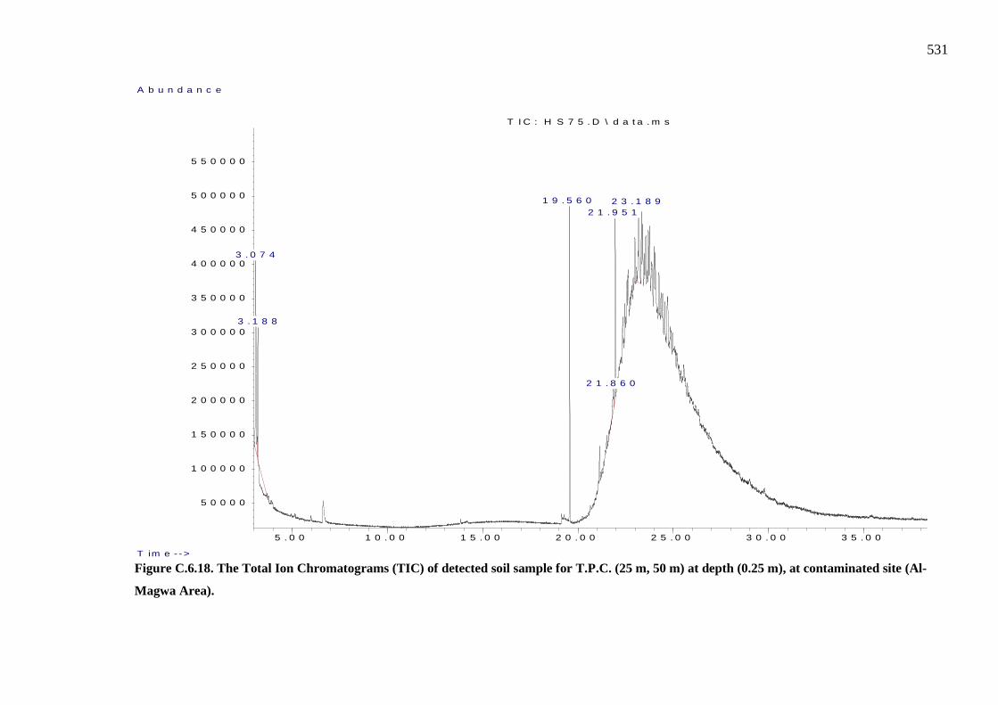
531
Figure C.6.18. The Total Ion Chromatograms (TIC) of detected soil sample for T.P.C. (25 m, 50 m) at depth (0.25 m), at contaminated site (Al-
Magwa Area).
5 . 0 0 1 0 . 0 0 1 5 . 0 0 2 0 . 0 0 2 5 . 0 0 3 0 . 0 0 3 5 . 0 0
5 0 0 0 0
1 0 0 0 0 0
1 5 0 0 0 0
2 0 0 0 0 0
2 5 0 0 0 0
3 0 0 0 0 0
3 5 0 0 0 0
4 0 0 0 0 0
4 5 0 0 0 0
5 0 0 0 0 0
5 5 0 0 0 0
T im e - - >
A b u n d a n c e
T I C : H S 7 5 . D \ d a t a . m s
3 . 0 7 4
3 . 1 8 8
1 9 . 5 6 0
2 1 . 8 6 0
2 1 . 9 5 12 3 . 1 8 9

532
Table C.6.43. The results of detected sample with TPH which tested by GC-MS instrument for T.P.C. (50 m, 50 m) at depth (0.25 m) of contaminated site (Al-Magwa Area).
Peak Ret. Time Chemical Composition of the TPH in
the Contaminated Soil Sample
Area Under the
Curve (m2)
Chemical Composition
Formula
Classification of the TPH based
on Aliphatic and Aromatic
Concentration of each TPH
Chemical Composition
Detected in the Contaminated
Soil Sample (µg/ml)
Concentration of each TPH
Chemical Composition Detected in
the Contaminated
Soil Sample (mg/kg)
Total
Concentration of the Total
TPH Compositions
Detected in the Contaminated
Soil Sample (mg/kg)
References
1 5.451 BV Dihydroxydimethylsilane 15785244 C2H8O2 ------- 177.791 59.263
3.506
(Dimethylsilanediol, n.d.)
2 13.276 BV C12H32O6Si3 Hexamethylhexaoxatrisilapentadecane
2868478 C12 Aromatic EC12 - EC16
10.518 3.506
(SCHEMBL2956430, n.d.)
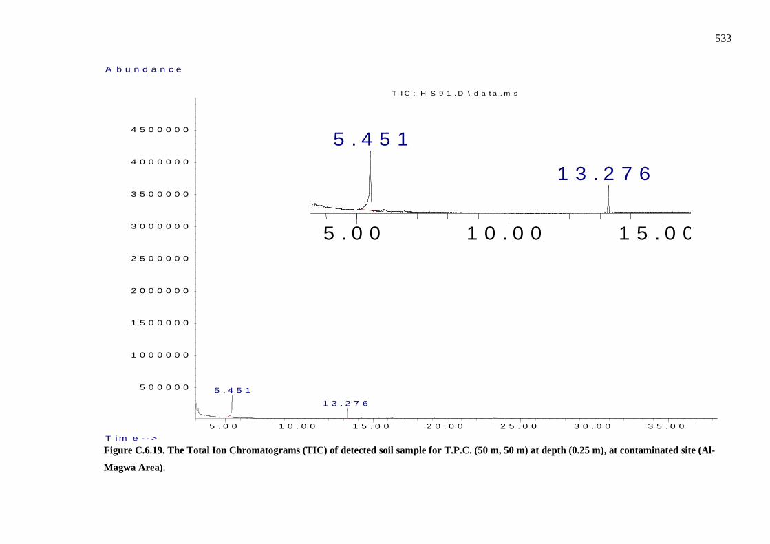
533
Figure C.6.19. The Total Ion Chromatograms (TIC) of detected soil sample for T.P.C. (50 m, 50 m) at depth (0.25 m), at contaminated site (Al-
Magwa Area).
5 . 0 0 1 0 . 0 0 1 5 . 0 0 2 0 . 0 0 2 5 . 0 0 3 0 . 0 0 3 5 . 0 0
5 0 0 0 0 0
1 0 0 0 0 0 0
1 5 0 0 0 0 0
2 0 0 0 0 0 0
2 5 0 0 0 0 0
3 0 0 0 0 0 0
3 5 0 0 0 0 0
4 0 0 0 0 0 0
4 5 0 0 0 0 0
T i m e - - >
A b u n d a n c e
T I C : H S 9 1 . D \ d a t a . m s
5 . 4 5 1
1 3 . 2 7 6
5 . 0 0 1 0 . 0 0 1 5 . 0 0 2 0 . 0 0 2 5 . 0 0 3 0 . 0 0 3 5 . 0 0
5 0 0 0 0 0
1 0 0 0 0 0 0
1 5 0 0 0 0 0
2 0 0 0 0 0 0
2 5 0 0 0 0 0
3 0 0 0 0 0 0
3 5 0 0 0 0 0
4 0 0 0 0 0 0
4 5 0 0 0 0 0
T i m e - - >
A b u n d a n c e
T I C : H S 9 1 . D \ d a t a . m s
5 . 4 5 1
1 3 . 2 7 6

534
Table C.6.44. The results of detected soil sample with TPH which tested by GC-MS instrument for T.P.C. (0 m, 75 m) at depth (0.25 m) of contaminated site (Al-Magwa Area).
Peak Ret. Time Chemical Composition of
the TPH in the Contaminated Soil Sample
Area Under
the Curve (m2)
Chemical Composition
Formula
Classification of the
TPH based on Aliphatic and Aromatic
Concentration of each TPH
Chemical Composition Detected in
the Contaminated
Soil Sample (µg/ml)
Concentration of each TPH
Chemical Composition Detected in
the Contaminated
Soil Sample (mg/kg)
Total
Concentration of the Total
TPH Compositions
Detected in the Contaminated
Soil Sample (mg/kg)
References
1 18.663 PV pentadecane 3907621 C15H32 Aliphatic EC12 - EC16
23.97 7.99
225.1
(Pentadecane, n.d.)
2 19.490 BV Hexadecane 5137019 C16H34 Aliphatic EC16 - EC35 39.896 13.298 (Hexadecane, n.d.)
3 19.874 PV Tridecane 6492353 C13H28 Aliphatic EC12 - EC16 57.448 19.149 (Tridecane, n.d.)
4 20.263 VV Heptadecane 6613165 C17H36 Aliphatic EC16 - EC35 59.012 19.670 (Heptadecane, n.d.)
5 20.311 PV Tetramethylpentadecane 3479945 C19H40 Aliphatic EC16 - EC35 18.437 6.145 (Pristane, n.d.)
6 20.995 VV Octadecane 6264583 C18H38 Aliphatic EC16 - EC35
54.498 18.166
(Octadecane, n.d.)
7 21.069 VV Tetramethylhexadecane 7623443 C20H42 Aliphatic EC16 - EC35
72.095 24.031
(Two, 6, 10, 14-tetramethylhexadecane,
n.d.) 8 21.648 PV Tetradecanoicacid ester 3560588 C28H56O2 Aliphatic EC16 - EC35 19.481 6.493 (Tetradecyl myristate, n.d.)
9 21.689 VV Nonadecane 7171546 C19H40 Aliphatic EC16 - EC35 66.243 22.081 (Nonadecane, n.d.)
10 22.350 VV Eicosane 8988373 C20H42 Aliphatic EC16 - EC35 89.771 29.923 (Icosane, n.d.)
11 22.647 VV Dimethyldibenzothiophene 5629771 C14H12S Aromatic EC12 - EC16
46.277 15.425
(Dimethyldibenzothiophene, n.d.)
12 22.848 VV 9,10-dimethylanthracene 5432648 C16H14 Aromatic EC16 - EC21
43.724 14.574
(Nine, 10-dimethylanthracene, n.d.)
13 22.983 VV Heneicosane 5772541 C21H44 Aliphatic EC16 - EC35 48.126 16.042 (Heneicosane, n.d.)
14 23.598 PV Heptadecane 4862296 C17H36 Aliphatic EC16 - EC35 36.338 12.112 (Heptadecane, n.d.)
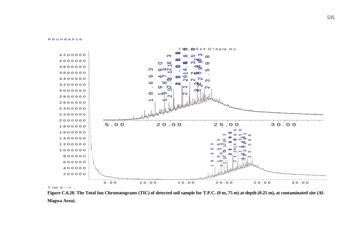
535
Figure C.6.20. The Total Ion Chromatograms (TIC) of detected soil sample for T.P.C. (0 m, 75 m) at depth (0.25 m), at contaminated site (Al-
Magwa Area).
5 . 0 0 1 0 . 0 0 1 5 . 0 0 2 0 . 0 0 2 5 . 0 0 3 0 . 0 0
2 0 0 0 0 0
4 0 0 0 0 0
6 0 0 0 0 0
8 0 0 0 0 0
1 0 0 0 0 0 0
1 2 0 0 0 0 0
1 4 0 0 0 0 0
1 6 0 0 0 0 0
1 8 0 0 0 0 0
2 0 0 0 0 0 0
2 2 0 0 0 0 0
2 4 0 0 0 0 0
2 6 0 0 0 0 0
2 8 0 0 0 0 0
3 0 0 0 0 0 0
3 2 0 0 0 0 0
3 4 0 0 0 0 0
3 6 0 0 0 0 0
3 8 0 0 0 0 0
4 0 0 0 0 0 0
4 2 0 0 0 0 0
T i m e - - >
A b u n d a n c e
T I C : H S 2 4 . D \ d a t a . m s
18
.6
63
19
.4
90
19
.8
74
20
.2
63
20
.3
11
20
.9
95
21
.0
69
21
.6
48
21
.6
89
22
.3
50
22
.6
47
22
.8
48
22
.9
83
23
.5
98

536
Table C.6.45. The results of detected soil sample with TPH which tested by GC-MS instrument for T.P.C. (100 m, 75 m) at depth (0.25 m) of contaminated site (Al-Magwa Area).
Peak Ret. Time Chemical Composition of
the TPH in the Contaminated Soil Sample
Area Under the
Curve (m2)
Chemical Composition
Formula
Classification of the
TPH based on Aliphatic and Aromatic
Concentration of each TPH
Chemical Composition Detected in
the Contaminated
Soil Sample (µg/ml)
Concentration of each TPH
Chemical Composition Detected in
the Contaminated
Soil Sample (mg/kg)
Total
Concentration of the Total
TPH Compositions
Detected in the
Contaminated Soil Sample
(mg/kg)
References
1 20.654 PV Trimethylpentadecane 12963837 C18H38 Aliphatic EC16 - EC35
141.253 47.08433
1271.038
(Two, 6, 10-Trimethylpentadecane, n.d.)
2 21.075 VV Tridecane 9065115 C13H28 Aliphatic EC12 - EC16
90.765 30.255
(Tridecane, n.d.)
3 21.129 VV Di-p-tolylacetylene 15615129 C16H14 Aromatic EC16 – EC21
175.588 58.52933
(Di-p-Tolylacetylene, n.d.)
4 21.870 VV Octadecane 23651142 C18H38 Aliphatic EC16 - EC35
279.654 93.218
(Octadecane, n.d.)
5 21.956 VV Di-p-tolylacetylene 42350166 C16H14 Aromatic EC16 – EC21
521.807 173.9357
(Di-p-Tolylacetylene, n.d.)
6 22.627 VV Nonadecane 26768203 C19H40 Aliphatic EC16 - EC35
320.020 106.6733
(Nonadecane, n.d.)
7 22.997 VV 1-methylphenanthrene 13197525 C15H12 Aromatic EC12 - EC16
144.280 48.09333
(Methylphenanthrene, n.d.)
8 23.153 VV 2-Methylanthracene 14894942 C15H12 Aromatic EC12 - EC16
166.261 55.42033
(Two-Methylanthracene, n.d.)
9 23.340 VV n-Eicosane 30374049 C20H42 Aliphatic EC16 - EC35
366.716 122.2387
(Icosane, n.d.)
10 23.399 VV 2,7-Dimethylbenzothiophene 21000368 C10H10S
Aromatic EC10 - EC12 245.327
81.77567 (Dimethylbenzothiophene,
2016)
11 23.565 VV 1,7-
Dimethylbenzothiophene 26261193 C10H10S Aromatic EC10 - EC12
313.454 104.4847
(Dimethylbenzothiophene, 2016)
12 23.701 VV Dimethylbenzothiopehene 22899828 C10H10S Aromatic EC10 - EC12
269.925 89.975
(Dimethylbenzothiophene, 2016)
13 23.763 VV 3,7-Dimethylbenzothiophene 28309191 C10H10S Aromatic EC10 - EC12 339.976 113.3253
(Dimethylbenzothiophene, 2016)
14 23.897 VV ---------- 33219713 ------ ---------
403.567 134.5223
---------
15 24.067 VV n-Cetane 24617097 C16H34 Aliphatic EC16 - EC35
292.163 97.38767
(Hexadecane, n.d.)
16 24.857 BV Docosane 13324585 C22H46 Aliphatic EC16 - EC35
145.925 48.64167
(Docosane, n.d.)
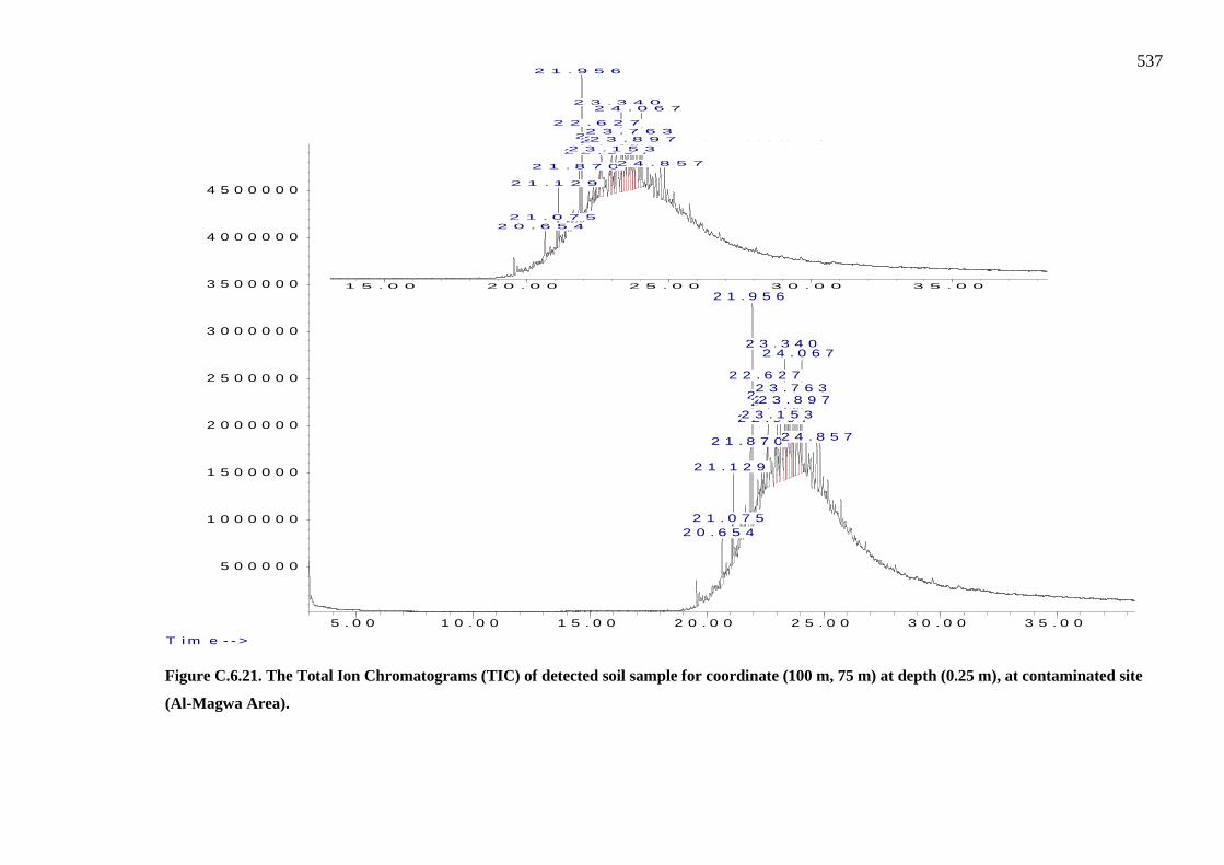
537
Figure C.6.21. The Total Ion Chromatograms (TIC) of detected soil sample for coordinate (100 m, 75 m) at depth (0.25 m), at contaminated site
(Al-Magwa Area).
5 . 0 0 1 0 . 0 0 1 5 . 0 0 2 0 . 0 0 2 5 . 0 0 3 0 . 0 0 3 5 . 0 0
5 0 0 0 0 0
1 0 0 0 0 0 0
1 5 0 0 0 0 0
2 0 0 0 0 0 0
2 5 0 0 0 0 0
3 0 0 0 0 0 0
3 5 0 0 0 0 0
4 0 0 0 0 0 0
4 5 0 0 0 0 0
T i m e - - >
A b u n d a n c e
T I C : H S 1 0 7 . D \ d a t a . m s
2 0 . 6 5 42 1 . 0 7 5
2 1 . 1 2 9
2 1 . 8 7 0
2 1 . 9 5 6
2 2 . 6 2 7
2 2 . 9 9 72 3 . 1 5 3
2 3 . 3 4 0
2 3 . 3 9 92 3 . 5 6 52 3 . 7 0 12 3 . 7 6 32 3 . 8 9 7
2 4 . 0 6 7
2 4 . 8 5 7

538
Table C.6.46. The results of detected soil sample with TPH which tested by GC-MS instrument for T.P.C. (75 m, 100 m) at depth (0.25 m) of contaminated site (Al-Magwa Area).
Peak Ret. Time
Chemical Composition of the TPH in the
Contaminated Soil Sample
Area Under the
Curve (m2)
Chemical Composition
Formula
Classification of the
TPH based on Aliphatic and Aromatic
Concentration of each TPH
Chemical Composition
Detected in the Contaminated
Soil Sample (µg/ml)
Concentration of each TPH
Chemical Composition
Detected in the Contaminated
Soil Sample (mg/kg)
Total
Concentration of the Total
TPH Compositions
Detected in the Contaminated
Soil Sample (mg/kg)
References
1 19.563 PV BHT 10151413 C15H24 Aromatic EC12 - EC16 104.832
34.944
532.378
(BHT, n.d.)
2 20.655 VV n-Dodecane 10529797 C12H26 Aliphatic EC12 - EC16 109.733 36.57767
(Dodecane, n.d.)
3 21.130 VV Tetramethylpentadecane 21392696 C19H40 Aliphatic EC16 - EC35 250.407 83.469
(Pristane, n.d.)
4 21.959 VV Tetramethylhexadecane 13747617 C20H42 Aliphatic EC16 - EC35 151.403 50.46767
(Two, 6, 10, 14-tetramethylhexadecane, n.d.)
5 22.459 PV Di-p-tolylacetylene 51574611 C16H14 Aromatic EC16 – EC21
641.263 213.7543
(Di-p-Tolylacetylene, n.d.)
6 22.579 VV n-cetane 19765174 C16H34 Aliphatic EC16 - EC35 229.331 76.44367
(Hexadecane, n.d.)
7 23.339 VV β-Pregnane 10563236 C21H36 Aliphatic EC16 - EC35
110.166 36.722
(Pregnane, n.d.)

539
Figure C.6.22. The Total Ion Chromatograms (TIC) of detected soil sample for T.P.C. (75 m, 100 m) at depth (0.25 m), at contaminated site (Al-
Magwa Area).
5 . 0 0 1 0 . 0 0 1 5 . 0 0 2 0 . 0 0 2 5 . 0 0 3 0 . 0 0 3 5 . 0 0
5 0 0 0 0 0
1 0 0 0 0 0 0
1 5 0 0 0 0 0
2 0 0 0 0 0 0
2 5 0 0 0 0 0
3 0 0 0 0 0 0
3 5 0 0 0 0 0
4 0 0 0 0 0 0
4 5 0 0 0 0 0
T i m e - - >
A b u n d a n c e
T I C : H S 1 0 8 . D \ d a t a . m s
1 9 . 5 6 3
2 0 . 6 5 5
2 1 . 1 3 0
2 1 . 9 5 9
2 2 . 4 5 9
2 2 . 5 7 92 3 . 3 3 9

540
At depth (0.5 m) at contaminated site
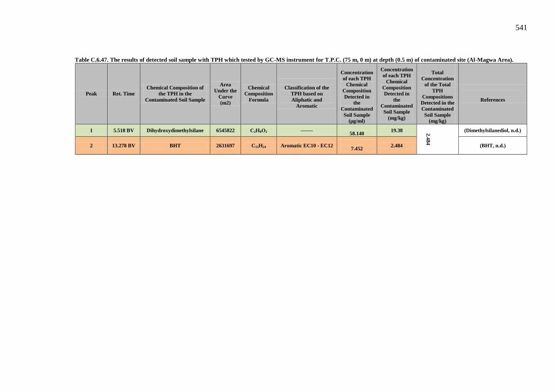
541
Table C.6.47. The results of detected soil sample with TPH which tested by GC-MS instrument for T.P.C. (75 m, 0 m) at depth (0.5 m) of contaminated site (Al-Magwa Area).
Peak Ret. Time Chemical Composition of
the TPH in the Contaminated Soil Sample
Area Under the
Curve (m2)
Chemical Composition
Formula
Classification of the
TPH based on Aliphatic and
Aromatic
Concentration of each TPH
Chemical Composition Detected in
the Contaminated
Soil Sample (µg/ml)
Concentration of each TPH
Chemical Composition Detected in
the Contaminated
Soil Sample (mg/kg)
Total
Concentration of the Total
TPH Compositions
Detected in the Contaminated
Soil Sample (mg/kg)
References
1 5.518 BV Dihydroxydimethylsilane 6545822 C2H8O2 ------- 58.140
19.38
2.484
(Dimethylsilanediol, n.d.)
2 13.278 BV BHT 2631697 C15H24 Aromatic EC10 - EC12 7.452 2.484 (BHT, n.d.)
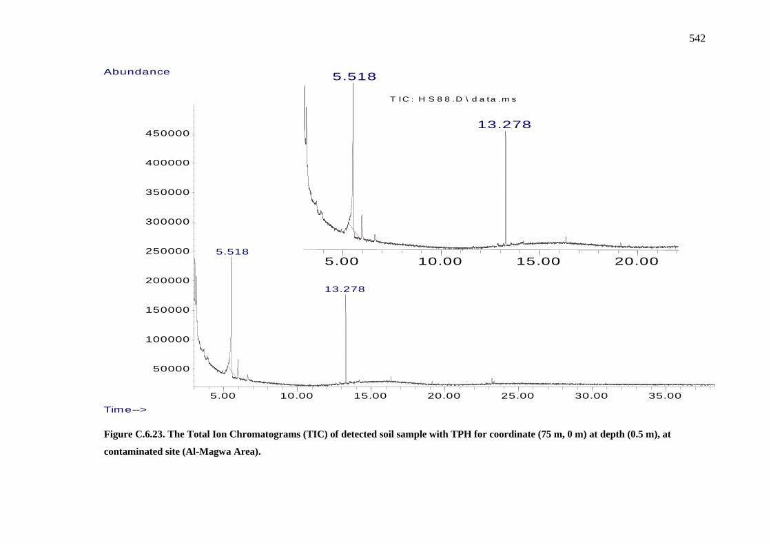
542
Figure C.6.23. The Total Ion Chromatograms (TIC) of detected soil sample with TPH for coordinate (75 m, 0 m) at depth (0.5 m), at
contaminated site (Al-Magwa Area).
5.00 10.00 15.00 20.00 25.00 30.00 35.00
50000
100000
150000
200000
250000
300000
350000
400000
450000
Time-->
Abundance
T IC : H S 8 8 .D \ d a ta .m s
5.518
13.278
5.00 10.00 15.00 20.00 25.00 30.00 35.00
50000
100000
150000
200000
250000
300000
350000
400000
450000
Time-->
Abundance
T IC : H S 8 8 .D \ d a ta .m s
5.518
13.278

543
Not Detected samples with TPH at contaminated site At Depth (0.0 m)
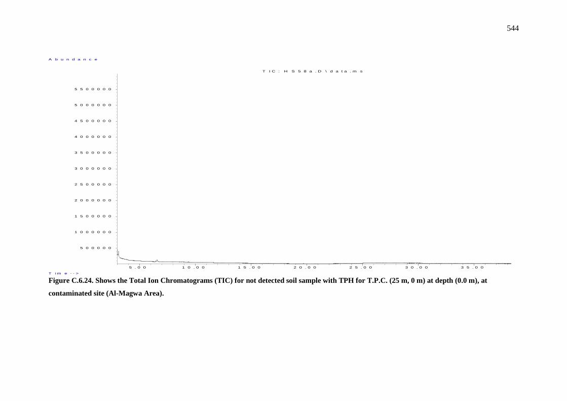
544
Figure C.6.24. Shows the Total Ion Chromatograms (TIC) for not detected soil sample with TPH for T.P.C. (25 m, 0 m) at depth (0.0 m), at
contaminated site (Al-Magwa Area).
5 . 0 0 1 0 . 0 0 1 5 . 0 0 2 0 . 0 0 2 5 . 0 0 3 0 . 0 0 3 5 . 0 0
5 0 0 0 0 0
1 0 0 0 0 0 0
1 5 0 0 0 0 0
2 0 0 0 0 0 0
2 5 0 0 0 0 0
3 0 0 0 0 0 0
3 5 0 0 0 0 0
4 0 0 0 0 0 0
4 5 0 0 0 0 0
5 0 0 0 0 0 0
5 5 0 0 0 0 0
T i m e - - >
A b u n d a n c e
T I C : H S 5 8 a . D \ d a t a . m s
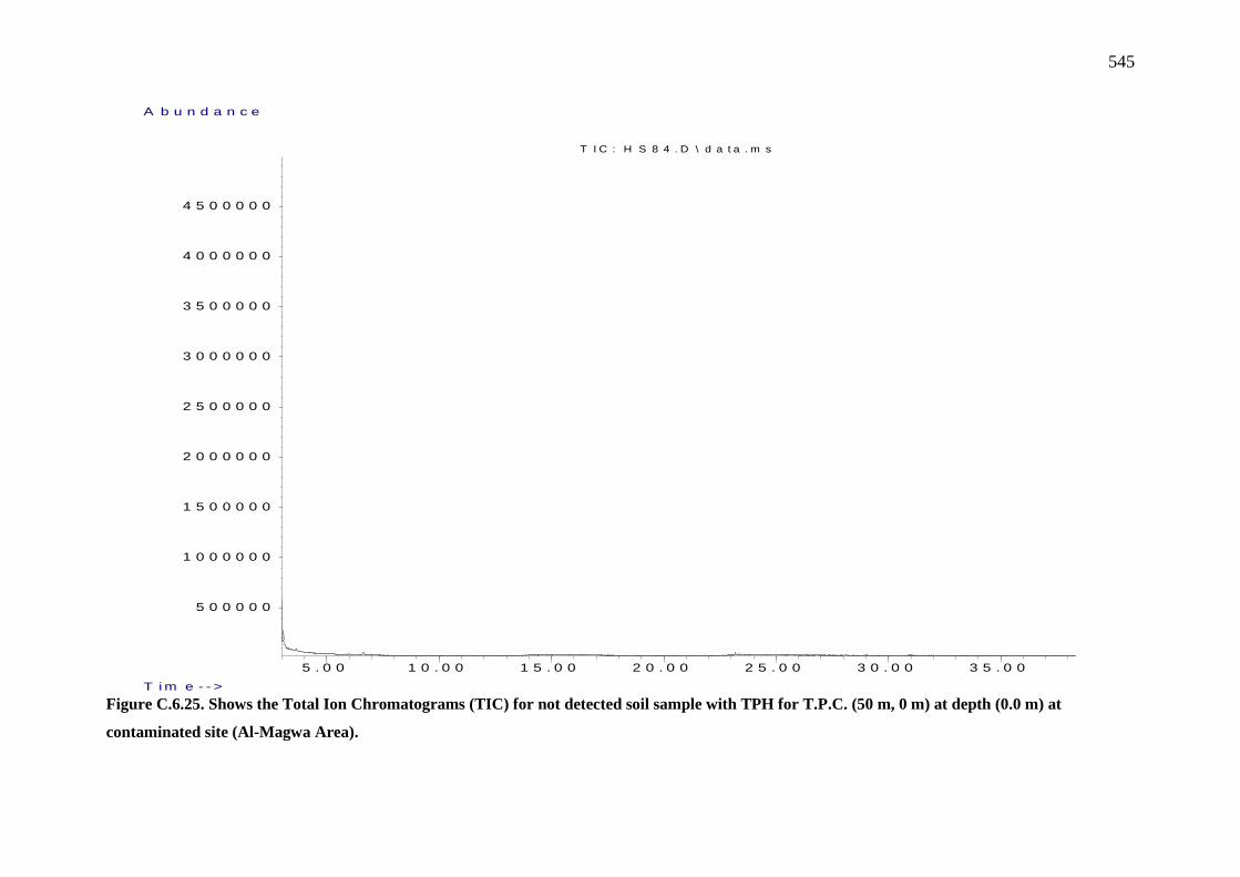
545
Figure C.6.25. Shows the Total Ion Chromatograms (TIC) for not detected soil sample with TPH for T.P.C. (50 m, 0 m) at depth (0.0 m) at
contaminated site (Al-Magwa Area).
5 . 0 0 1 0 . 0 0 1 5 . 0 0 2 0 . 0 0 2 5 . 0 0 3 0 . 0 0 3 5 . 0 0
5 0 0 0 0 0
1 0 0 0 0 0 0
1 5 0 0 0 0 0
2 0 0 0 0 0 0
2 5 0 0 0 0 0
3 0 0 0 0 0 0
3 5 0 0 0 0 0
4 0 0 0 0 0 0
4 5 0 0 0 0 0
T i m e - - >
A b u n d a n c e
T I C : H S 8 4 . D \ d a t a . m s

546
Figure C.6.26. Shows the Total Ion Chromatograms (TIC) for not detected soil sample with TPH for T.P.C. (50 m, 25 m) at depth (0.0 m), at
contaminated site (Al-Magwa Area).
5 .0 0 1 0 .0 0 1 5 .0 0 2 0 .0 0 2 5 .0 0 3 0 .0 0
2 0 0 0 0 0
4 0 0 0 0 0
6 0 0 0 0 0
8 0 0 0 0 0
1 0 0 0 0 0 0
1 2 0 0 0 0 0
1 4 0 0 0 0 0
1 6 0 0 0 0 0
1 8 0 0 0 0 0
2 0 0 0 0 0 0
2 2 0 0 0 0 0
2 4 0 0 0 0 0
2 6 0 0 0 0 0
2 8 0 0 0 0 0
3 0 0 0 0 0 0
3 2 0 0 0 0 0
3 4 0 0 0 0 0
3 6 0 0 0 0 0
3 8 0 0 0 0 0
4 0 0 0 0 0 0
4 2 0 0 0 0 0
4 4 0 0 0 0 0
4 6 0 0 0 0 0
T i m e - - >
A b u n d a n c e
T I C : H S 4 1 . D \ d a t a . m s
547
Figure C.6.27. Shows the Total Ion Chromatograms (TIC) for not detected soil sample with TPH for T.P.C. (0 m, 50 m) at depth (0.0 m), at
contaminated site (Al-Magwa Area).
5 .0 0 1 0 . 0 0 1 5 . 0 0 2 0 . 0 0 2 5 . 0 0 3 0 . 0 0
2 0 0 0 0 0
4 0 0 0 0 0
6 0 0 0 0 0
8 0 0 0 0 0
1 0 0 0 0 0 0
1 2 0 0 0 0 0
1 4 0 0 0 0 0
1 6 0 0 0 0 0
1 8 0 0 0 0 0
2 0 0 0 0 0 0
2 2 0 0 0 0 0
2 4 0 0 0 0 0
2 6 0 0 0 0 0
2 8 0 0 0 0 0
3 0 0 0 0 0 0
3 2 0 0 0 0 0
3 4 0 0 0 0 0
3 6 0 0 0 0 0
3 8 0 0 0 0 0
4 0 0 0 0 0 0
4 2 0 0 0 0 0
4 4 0 0 0 0 0
4 6 0 0 0 0 0
4 8 0 0 0 0 0
T i m e - - >
A b u n d a n c e
T I C : H S 4 8 . D \ d a t a . m s

548
Figure C.6.28. Shows the Total Ion Chromatograms (TIC) for not detected soil sample with TPH for T.P.C. (100 m, 75 m) at depth (0.0 m),
at contaminated site (Al-Magwa Area).
5 .0 0 1 0 .0 0 1 5 .0 0 2 0 .0 0 2 5 .0 0 3 0 .0 0
2 0 0 0 0 0
4 0 0 0 0 0
6 0 0 0 0 0
8 0 0 0 0 0
1 0 0 0 0 0 0
1 2 0 0 0 0 0
1 4 0 0 0 0 0
1 6 0 0 0 0 0
1 8 0 0 0 0 0
2 0 0 0 0 0 0
2 2 0 0 0 0 0
2 4 0 0 0 0 0
2 6 0 0 0 0 0
2 8 0 0 0 0 0
3 0 0 0 0 0 0
3 2 0 0 0 0 0
3 4 0 0 0 0 0
3 6 0 0 0 0 0
3 8 0 0 0 0 0
4 0 0 0 0 0 0
4 2 0 0 0 0 0
4 4 0 0 0 0 0
T i m e - - >
A b u n d a n c e
T I C : H S 4 2 . D \ d a t a . m s

549
At depth (0.25 m)

550
Figure C.6.29. Shows the Total Ion Chromatograms (TIC) for not detected soil sample with TPH for T.P.C. (0 m, 0 m) at depth (0.25 m), at
contaminated site (Al-Magwa Area).
5 . 0 0 1 0 . 0 0 1 5 . 0 0 2 0 . 0 0 2 5 . 0 0 3 0 . 0 0
5 0 0 0 0
1 0 0 0 0 0
1 5 0 0 0 0
2 0 0 0 0 0
2 5 0 0 0 0
3 0 0 0 0 0
3 5 0 0 0 0
4 0 0 0 0 0
4 5 0 0 0 0
5 0 0 0 0 0
5 5 0 0 0 0
6 0 0 0 0 0
6 5 0 0 0 0
7 0 0 0 0 0
7 5 0 0 0 0
8 0 0 0 0 0
8 5 0 0 0 0
9 0 0 0 0 0
9 5 0 0 0 0
1 0 0 0 0 0 0
1 0 5 0 0 0 0
1 1 0 0 0 0 0
1 1 5 0 0 0 0
1 2 0 0 0 0 0
1 2 5 0 0 0 0
1 3 0 0 0 0 0
1 3 5 0 0 0 0
T im e - - >
A b u n d a n c e
T I C : H S 6 . D \ d a t a . m s
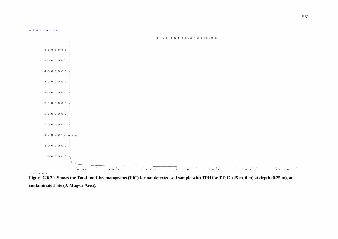
551
Figure C.6.30. Shows the Total Ion Chromatograms (TIC) for not detected soil sample with TPH for T.P.C. (25 m, 0 m) at depth (0.25 m), at
contaminated site (A-Magwa Area).
5 . 0 0 1 0 . 0 0 1 5 . 0 0 2 0 . 0 0 2 5 . 0 0 3 0 . 0 0 3 5 . 0 0
5 0 0 0 0 0
1 0 0 0 0 0 0
1 5 0 0 0 0 0
2 0 0 0 0 0 0
2 5 0 0 0 0 0
3 0 0 0 0 0 0
3 5 0 0 0 0 0
4 0 0 0 0 0 0
4 5 0 0 0 0 0
5 0 0 0 0 0 0
5 5 0 0 0 0 0
T i m e - - >
A b u n d a n c e
T I C : H S 5 9 a . D \ d a t a . m s
3 . 0 5 0
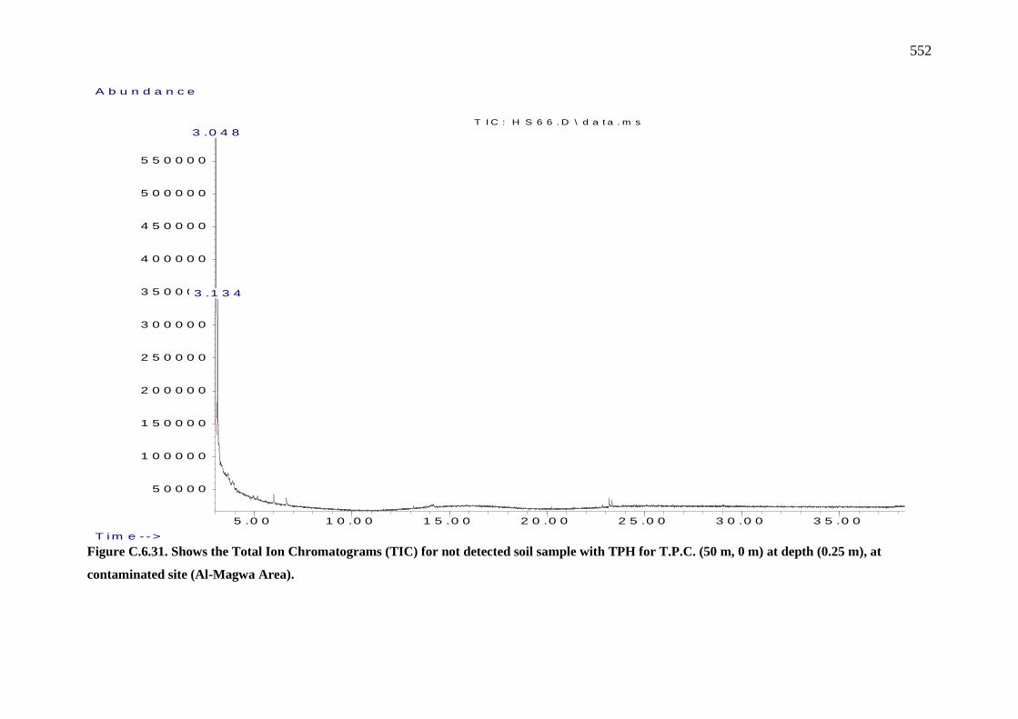
552
Figure C.6.31. Shows the Total Ion Chromatograms (TIC) for not detected soil sample with TPH for T.P.C. (50 m, 0 m) at depth (0.25 m), at
contaminated site (Al-Magwa Area).
5 .0 0 1 0 .0 0 1 5 .0 0 2 0 .0 0 2 5 .0 0 3 0 .0 0 3 5 .0 0
5 0 0 0 0
1 0 0 0 0 0
1 5 0 0 0 0
2 0 0 0 0 0
2 5 0 0 0 0
3 0 0 0 0 0
3 5 0 0 0 0
4 0 0 0 0 0
4 5 0 0 0 0
5 0 0 0 0 0
5 5 0 0 0 0
T im e - - >
A b u n d a n c e
T I C : H S 6 6 . D \ d a t a . m s 3 .0 4 8
3 .1 3 4

553
Figure C.6.32. Shows the Total Ion Chromatograms (TIC) for not detected soil sample with TPH for T.P.C. (75 m, 0 m) at depth (0.25 m), at
contaminated site (Al-Magwa Area).
5 .00 10 .00 15 .00 20 .00 25 .00 30 .00
200000
400000
600000
800000
1000000
1200000
1400000
1600000
1800000
2000000
2200000
2400000
2600000
2800000
3000000
3200000
3400000
3600000
3800000
T im e- ->
A bundanc e
T IC : H S 3 0 .D \ d a ta .m s
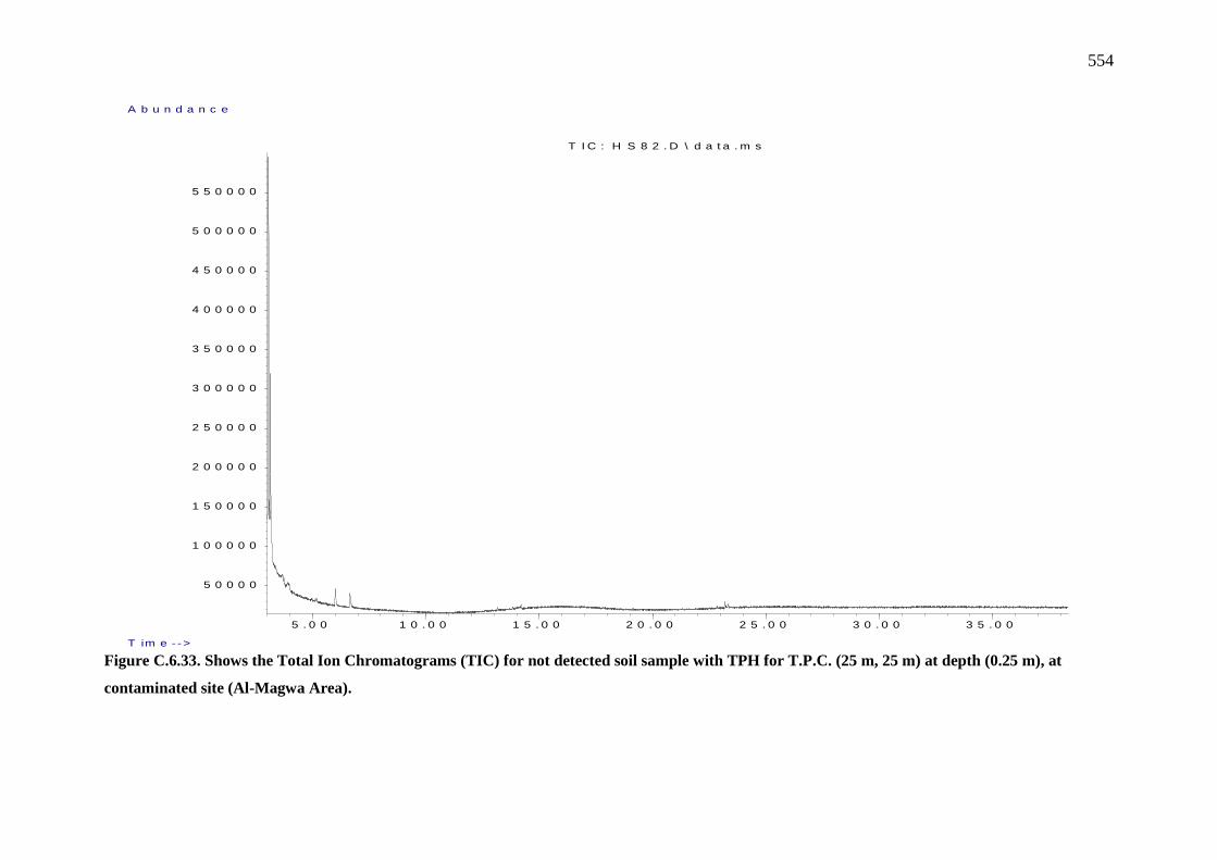
554
Figure C.6.33. Shows the Total Ion Chromatograms (TIC) for not detected soil sample with TPH for T.P.C. (25 m, 25 m) at depth (0.25 m), at
contaminated site (Al-Magwa Area).
5 . 0 0 1 0 . 0 0 1 5 . 0 0 2 0 . 0 0 2 5 . 0 0 3 0 . 0 0 3 5 . 0 0
5 0 0 0 0
1 0 0 0 0 0
1 5 0 0 0 0
2 0 0 0 0 0
2 5 0 0 0 0
3 0 0 0 0 0
3 5 0 0 0 0
4 0 0 0 0 0
4 5 0 0 0 0
5 0 0 0 0 0
5 5 0 0 0 0
T im e - - >
A b u n d a n c e
T I C : H S 8 2 . D \ d a t a . m s
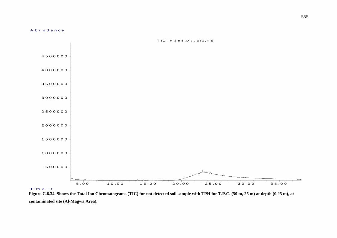
555
Figure C.6.34. Shows the Total Ion Chromatograms (TIC) for not detected soil sample with TPH for T.P.C. (50 m, 25 m) at depth (0.25 m), at
contaminated site (Al-Magwa Area).
5 . 0 0 1 0 . 0 0 1 5 . 0 0 2 0 . 0 0 2 5 . 0 0 3 0 . 0 0 3 5 . 0 0
5 0 0 0 0 0
1 0 0 0 0 0 0
1 5 0 0 0 0 0
2 0 0 0 0 0 0
2 5 0 0 0 0 0
3 0 0 0 0 0 0
3 5 0 0 0 0 0
4 0 0 0 0 0 0
4 5 0 0 0 0 0
T i m e - - >
A b u n d a n c e
T I C : H S 9 5 . D \ d a t a . m s

556
Figure C.6.35. Shows the Total Ion Chromatograms (TIC) for not detected soil sample with TPH for T.P.C. (100 m, 25 m) at depth (0.25 m), at
contaminated site (Al-Magwa Area).
5 . 0 0 1 0 . 0 0 1 5 . 0 0 2 0 . 0 0 2 5 . 0 0 3 0 . 0 0 3 5 . 0 0
5 0 0 0 0 0
1 0 0 0 0 0 0
1 5 0 0 0 0 0
2 0 0 0 0 0 0
2 5 0 0 0 0 0
3 0 0 0 0 0 0
3 5 0 0 0 0 0
4 0 0 0 0 0 0
4 5 0 0 0 0 0
5 0 0 0 0 0 0
5 5 0 0 0 0 0
T i m e - - >
A b u n d a n c e
T I C : H S 1 1 5 . D \ d a t a . m s
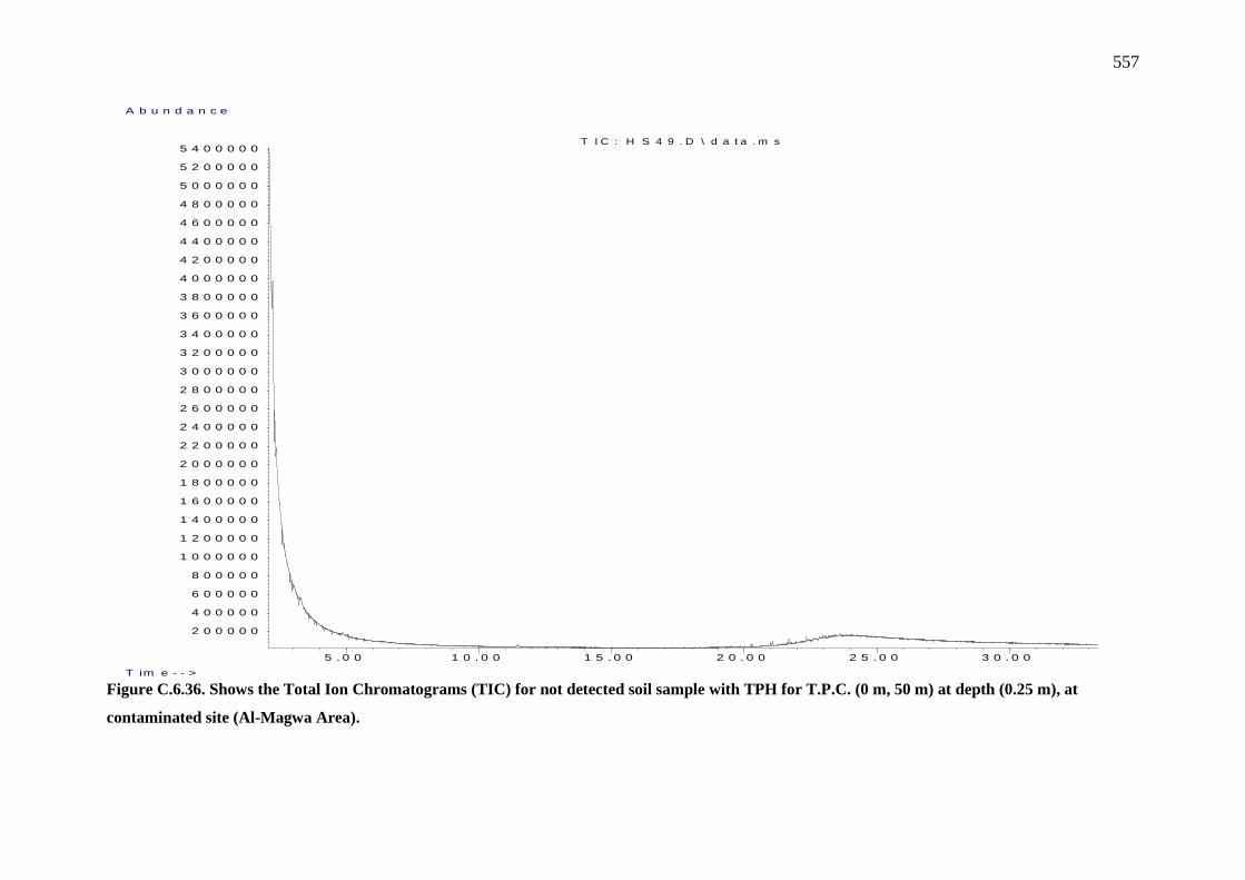
557
Figure C.6.36. Shows the Total Ion Chromatograms (TIC) for not detected soil sample with TPH for T.P.C. (0 m, 50 m) at depth (0.25 m), at
contaminated site (Al-Magwa Area).
5 . 0 0 1 0 . 0 0 1 5 . 0 0 2 0 . 0 0 2 5 . 0 0 3 0 . 0 0
2 0 0 0 0 0
4 0 0 0 0 0
6 0 0 0 0 0
8 0 0 0 0 0
1 0 0 0 0 0 0
1 2 0 0 0 0 0
1 4 0 0 0 0 0
1 6 0 0 0 0 0
1 8 0 0 0 0 0
2 0 0 0 0 0 0
2 2 0 0 0 0 0
2 4 0 0 0 0 0
2 6 0 0 0 0 0
2 8 0 0 0 0 0
3 0 0 0 0 0 0
3 2 0 0 0 0 0
3 4 0 0 0 0 0
3 6 0 0 0 0 0
3 8 0 0 0 0 0
4 0 0 0 0 0 0
4 2 0 0 0 0 0
4 4 0 0 0 0 0
4 6 0 0 0 0 0
4 8 0 0 0 0 0
5 0 0 0 0 0 0
5 2 0 0 0 0 0
5 4 0 0 0 0 0
T im e - - >
A b u n d a n c e
T I C : H S 4 9 . D \ d a t a . m s
558
Figure C.6.37. Shows the Total Ion Chromatograms (TIC) for not detected soil sample with TPH for T.P.C. (100 m, 50 m) at depth (0.25 m), at
contaminated site (Al-Magwa Area).
5 .0 0 1 0 .0 0 1 5 .0 0 2 0 .0 0 2 5 .0 0 3 0 .0 0
2 0 0 0 0 0
4 0 0 0 0 0
6 0 0 0 0 0
8 0 0 0 0 0
1 0 0 0 0 0 0
1 2 0 0 0 0 0
1 4 0 0 0 0 0
1 6 0 0 0 0 0
1 8 0 0 0 0 0
2 0 0 0 0 0 0
2 2 0 0 0 0 0
2 4 0 0 0 0 0
2 6 0 0 0 0 0
2 8 0 0 0 0 0
3 0 0 0 0 0 0
3 2 0 0 0 0 0
3 4 0 0 0 0 0
3 6 0 0 0 0 0
3 8 0 0 0 0 0
4 0 0 0 0 0 0
4 2 0 0 0 0 0
4 4 0 0 0 0 0
4 6 0 0 0 0 0
T i m e - - >
A b u n d a n c e
T I C : H S 3 8 . D \ d a t a . m s
559
Figure. C.6.38. Shows the Total Ion Chromatograms (TIC) for not detected soil sample with TPH for T.P.C. (25 m, 75 m) at depth (0.25 m), at
contaminated site (Al-Magwa Area).
5 . 0 0 1 0 . 0 0 1 5 . 0 0 2 0 . 0 0 2 5 . 0 0 3 0 . 0 0 3 5 . 0 0
5 0 0 0 0 0
1 0 0 0 0 0 0
1 5 0 0 0 0 0
2 0 0 0 0 0 0
2 5 0 0 0 0 0
3 0 0 0 0 0 0
3 5 0 0 0 0 0
4 0 0 0 0 0 0
4 5 0 0 0 0 0
T i m e - - >
A b u n d a n c e
T I C : H S 8 6 . D \ d a t a . m s

560
Figure C.6.39. Shows the Total Ion Chromatograms (TIC) for not detected soil sample with TPH for T.P.C. (50 m, 75 m) at depth (0.25 m) at
contaminated site (Al-Magwa Area).
5 . 0 0 1 0 . 0 0 1 5 . 0 0 2 0 . 0 0 2 5 . 0 0 3 0 . 0 0
2 0 0 0 0 0
4 0 0 0 0 0
6 0 0 0 0 0
8 0 0 0 0 0
1 0 0 0 0 0 0
1 2 0 0 0 0 0
1 4 0 0 0 0 0
1 6 0 0 0 0 0
1 8 0 0 0 0 0
2 0 0 0 0 0 0
2 2 0 0 0 0 0
2 4 0 0 0 0 0
2 6 0 0 0 0 0
2 8 0 0 0 0 0
3 0 0 0 0 0 0
3 2 0 0 0 0 0
T im e - - >
A b u n d a n c e
T I C : H S 1 3 . D \ d a t a . m s
561
Figure C.6.40. Shows the Total Ion Chromatograms (TIC) for not detected soil sample with TPH for T.P.C. (75 m, 75 m) at depth (0.25 m), at
contaminated site (Al-Magwa Area).
5 . 0 0 1 0 . 0 0 1 5 . 0 0 2 0 . 0 0 2 5 . 0 0 3 0 . 0 0
2 0 0 0 0 0
4 0 0 0 0 0
6 0 0 0 0 0
8 0 0 0 0 0
1 0 0 0 0 0 0
1 2 0 0 0 0 0
1 4 0 0 0 0 0
1 6 0 0 0 0 0
1 8 0 0 0 0 0
2 0 0 0 0 0 0
2 2 0 0 0 0 0
2 4 0 0 0 0 0
2 6 0 0 0 0 0
2 8 0 0 0 0 0
3 0 0 0 0 0 0
3 2 0 0 0 0 0
3 4 0 0 0 0 0
3 6 0 0 0 0 0
3 8 0 0 0 0 0
4 0 0 0 0 0 0
4 2 0 0 0 0 0
4 4 0 0 0 0 0
4 6 0 0 0 0 0
4 8 0 0 0 0 0
5 0 0 0 0 0 0
T i m e - - >
A b u n d a n c e
T I C : H S 4 5 . D \ d a t a . m s
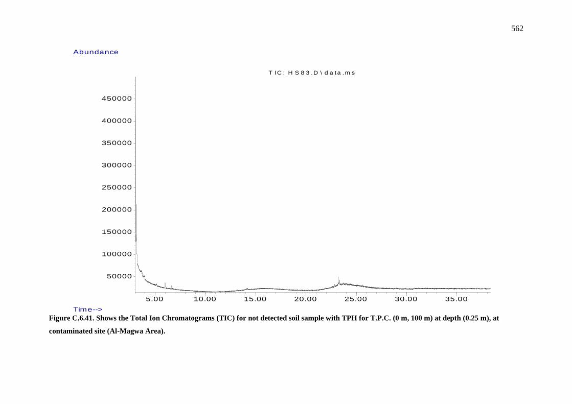
562
Figure C.6.41. Shows the Total Ion Chromatograms (TIC) for not detected soil sample with TPH for T.P.C. (0 m, 100 m) at depth (0.25 m), at
contaminated site (Al-Magwa Area).
5.00 10.00 15.00 20.00 25.00 30.00 35.00
50000
100000
150000
200000
250000
300000
350000
400000
450000
Time-->
Abundance
T IC : H S 8 3 .D \ d a ta .m s
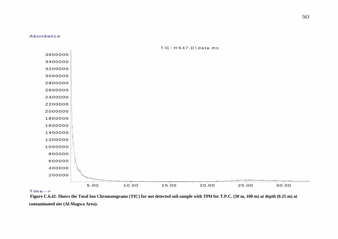
563
Figure C.6.42. Shows the Total Ion Chromatograms (TIC) for not detected soil sample with TPH for T.P.C. (50 m, 100 m) at depth (0.25 m) at
contaminated site (Al-Magwa Area).
5.00 10.00 15.00 20.00 25.00 30.00
200000
400000
600000
800000
1000000
1200000
1400000
1600000
1800000
2000000
2200000
2400000
2600000
2800000
3000000
3200000
3400000
3600000
T im e-->
Abundanc e
T IC : H S 4 7 .D \ d a ta .m s

564
Figure C.6.43. Shows the Total Ion Chromatograms (TIC) for not detected soil sample with TPH for T.P.C. (100 m, 100 m) at depth (0.25 m), at
contaminated site (Al-Magwa Area).
5 . 0 0 1 0 . 0 0 1 5 . 0 0 2 0 . 0 0 2 5 . 0 0 3 0 . 0 0 3 5 . 0 0
5 0 0 0 0 0
1 0 0 0 0 0 0
1 5 0 0 0 0 0
2 0 0 0 0 0 0
2 5 0 0 0 0 0
3 0 0 0 0 0 0
3 5 0 0 0 0 0
4 0 0 0 0 0 0
4 5 0 0 0 0 0
T i m e - - >
A b u n d a n c e
T I C : H S 1 0 5 . D \ d a t a . m s

565
At Depth (0.5 m)

566
Figure C.6.44. Shows the Total Ion Chromatograms (TIC) for not detected soil sample with TPH for T.P.C. (0 m, 0 m) at depth (0.5 m), at
contaminated site (Al-Magwa Area).
5 . 0 0 1 0 . 0 0 1 5 . 0 0 2 0 . 0 0 2 5 . 0 0 3 0 . 0 0 3 5 . 0 0
5 0 0 0 0 0
1 0 0 0 0 0 0
1 5 0 0 0 0 0
2 0 0 0 0 0 0
2 5 0 0 0 0 0
3 0 0 0 0 0 0
3 5 0 0 0 0 0
4 0 0 0 0 0 0
4 5 0 0 0 0 0
T im e - - >
A b u n d a n c e
T I C : H S 1 2 0 . D \ d a t a . m s
3 . 1 2 4

567
Figure C.6.45. Shows the Total Ion Chromatograms (TIC) for not detected soil sample with TPH for T.P.C. (25 m, 0 m) at depth (0.5 m), at
contaminated site (Al-Magwa Area).
5 . 0 0 1 0 . 0 0 1 5 . 0 0 2 0 . 0 0 2 5 . 0 0 3 0 . 0 0 3 5 . 0 0
5 0 0 0 0 0
1 0 0 0 0 0 0
1 5 0 0 0 0 0
2 0 0 0 0 0 0
2 5 0 0 0 0 0
3 0 0 0 0 0 0
3 5 0 0 0 0 0
4 0 0 0 0 0 0
4 5 0 0 0 0 0
5 0 0 0 0 0 0
5 5 0 0 0 0 0
T i m e - - >
A b u n d a n c e
T I C : H S 1 0 3 . D \ d a t a . m s
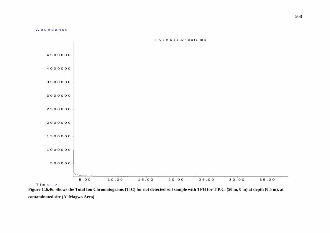
568
Figure C.6.46. Shows the Total Ion Chromatograms (TIC) for not detected soil sample with TPH for T.P.C. (50 m, 0 m) at depth (0.5 m), at
contaminated site (Al-Magwa Area).
5 . 0 0 1 0 . 0 0 1 5 . 0 0 2 0 . 0 0 2 5 . 0 0 3 0 . 0 0 3 5 . 0 0
5 0 0 0 0 0
1 0 0 0 0 0 0
1 5 0 0 0 0 0
2 0 0 0 0 0 0
2 5 0 0 0 0 0
3 0 0 0 0 0 0
3 5 0 0 0 0 0
4 0 0 0 0 0 0
4 5 0 0 0 0 0
T i m e - - >
A b u n d a n c e
T I C : H S 8 5 . D \ d a t a . m s

569
Figure C.6.47. Shows the Total Ion Chromatograms (TIC) for not detected soil sample with TPH for T.P.C. (100 m, 0 m) at depth (0.5 m),
at contaminated site (Al-Magwa Area).
5 . 0 0 1 0 . 0 0 1 5 . 0 0 2 0 . 0 0 2 5 . 0 0 3 0 . 0 0 3 5 . 0 0
5 0 0 0 0 0
1 0 0 0 0 0 0
1 5 0 0 0 0 0
2 0 0 0 0 0 0
2 5 0 0 0 0 0
3 0 0 0 0 0 0
3 5 0 0 0 0 0
4 0 0 0 0 0 0
4 5 0 0 0 0 0
T i m e - - >
A b u n d a n c e
T I C : H S 9 0 . D \ d a t a . m s

570
Figure C.6.48. Shows the Total Ion Chromatograms (TIC) for not detected soil sample with TPH for T.P.C. (0 m, 25 m) at depth (0.5 m), at
contaminated site (Al-Magwa Area).
5 . 0 0 1 0 . 0 0 1 5 . 0 0 2 0 . 0 0 2 5 . 0 0 3 0 . 0 0 3 5 . 0 0
5 0 0 0 0 0
1 0 0 0 0 0 0
1 5 0 0 0 0 0
2 0 0 0 0 0 0
2 5 0 0 0 0 0
3 0 0 0 0 0 0
3 5 0 0 0 0 0
4 0 0 0 0 0 0
4 5 0 0 0 0 0
T i m e - - >
A b u n d a n c e
T I C : H S 8 7 . D \ d a t a . m s

571
Figure C.6.49. Shows the Total Ion Chromatograms (TIC) for not detected soil sample with TPH for T.P.C. (25 m, 25 m) at depth (0.5 m), at
contaminated site (Al-MAgwa Area).
5 . 0 0 1 0 . 0 0 1 5 . 0 0 2 0 . 0 0 2 5 . 0 0 3 0 . 0 0 3 5 . 0 0
5 0 0 0 0 0
1 0 0 0 0 0 0
1 5 0 0 0 0 0
2 0 0 0 0 0 0
2 5 0 0 0 0 0
3 0 0 0 0 0 0
3 5 0 0 0 0 0
4 0 0 0 0 0 0
4 5 0 0 0 0 0
5 0 0 0 0 0 0
5 5 0 0 0 0 0
T i m e - - >
A b u n d a n c e
T I C : H S 1 0 7 . D \ d a t a . m s

572
Figure C.6.50. Shows the Total Ion Chromatograms (TIC) for not detected soil sample with TPH for T.P.C. (50 m, 25 m) at depth (0.5 m), at
contaminated site (Al-Magwa Area).
5 . 0 0 1 0 . 0 0 1 5 . 0 0 2 0 . 0 0 2 5 . 0 0 3 0 . 0 0 3 5 . 0 0
5 0 0 0 0 0
1 0 0 0 0 0 0
1 5 0 0 0 0 0
2 0 0 0 0 0 0
2 5 0 0 0 0 0
3 0 0 0 0 0 0
3 5 0 0 0 0 0
4 0 0 0 0 0 0
4 5 0 0 0 0 0
5 0 0 0 0 0 0
5 5 0 0 0 0 0
T i m e - - >
A b u n d a n c e
T I C : H S 1 0 7 . D \ d a t a . m s
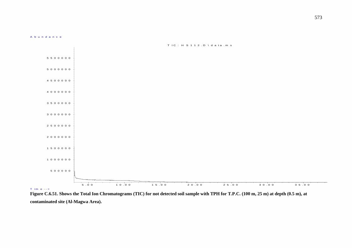
573
Figure C.6.51. Shows the Total Ion Chromatograms (TIC) for not detected soil sample with TPH for T.P.C. (100 m, 25 m) at depth (0.5 m), at
contaminated site (Al-Magwa Area).
5 . 0 0 1 0 . 0 0 1 5 . 0 0 2 0 . 0 0 2 5 . 0 0 3 0 . 0 0 3 5 . 0 0
5 0 0 0 0 0
1 0 0 0 0 0 0
1 5 0 0 0 0 0
2 0 0 0 0 0 0
2 5 0 0 0 0 0
3 0 0 0 0 0 0
3 5 0 0 0 0 0
4 0 0 0 0 0 0
4 5 0 0 0 0 0
5 0 0 0 0 0 0
5 5 0 0 0 0 0
T i m e - - >
A b u n d a n c e
T I C : H S 1 1 2 . D \ d a t a . m s

574
Figure C.6.52. Shows the Total Ion Chromatograms (TIC) for not detected soil sample with TPH for T.P.C. (0 m, 50 m) at depth (0.5 m), at
contaminated site (Al-Magwa Area).
5 . 0 0 1 0 . 0 0 1 5 . 0 0 2 0 . 0 0 2 5 . 0 0 3 0 . 0 0 3 5 . 0 0
5 0 0 0 0 0
1 0 0 0 0 0 0
1 5 0 0 0 0 0
2 0 0 0 0 0 0
2 5 0 0 0 0 0
3 0 0 0 0 0 0
3 5 0 0 0 0 0
4 0 0 0 0 0 0
4 5 0 0 0 0 0
5 0 0 0 0 0 0
5 5 0 0 0 0 0
T i m e - - >
A b u n d a n c e
T I C : H S 1 1 1 . D \ d a t a . m s
3 . 0 3 9
575
Figure C.6.53. Shows the Total Ion Chromatograms (TIC) for not detected soil sample with TPH for T.P.C. (25 m, 50 m) at depth (0.5 m), at
contaminated site (Al-Magwa Area).
5 . 0 0 1 0 . 0 0 1 5 . 0 0 2 0 . 0 0 2 5 . 0 0 3 0 . 0 0 3 5 . 0 0
5 0 0 0 0 0
1 0 0 0 0 0 0
1 5 0 0 0 0 0
2 0 0 0 0 0 0
2 5 0 0 0 0 0
3 0 0 0 0 0 0
3 5 0 0 0 0 0
4 0 0 0 0 0 0
4 5 0 0 0 0 0
T i m e - - >
A b u n d a n c e
T I C : H S 1 1 9 . D \ d a t a . m s

576
Figure C.6.54. Shows the Total Ion Chromatograms (TIC) for not detected soil sample with TPH for T.P.C. (50 m, 50 m) at depth (0.5 m), at
contaminated site (Al-Magwa Area).
5 . 0 0 1 0 . 0 0 1 5 . 0 0 2 0 . 0 0 2 5 . 0 0 3 0 . 0 0
2 0 0 0 0 0
4 0 0 0 0 0
6 0 0 0 0 0
8 0 0 0 0 0
1 0 0 0 0 0 0
1 2 0 0 0 0 0
1 4 0 0 0 0 0
1 6 0 0 0 0 0
1 8 0 0 0 0 0
2 0 0 0 0 0 0
2 2 0 0 0 0 0
2 4 0 0 0 0 0
2 6 0 0 0 0 0
2 8 0 0 0 0 0
3 0 0 0 0 0 0
3 2 0 0 0 0 0
3 4 0 0 0 0 0
3 6 0 0 0 0 0
3 8 0 0 0 0 0
4 0 0 0 0 0 0
4 2 0 0 0 0 0
4 4 0 0 0 0 0
4 6 0 0 0 0 0
4 8 0 0 0 0 0
T i m e - - >
A b u n d a n c e
T I C : H S 8 . D \ d a t a . m s

577
Figure C.6.55. Shows the Total Ion Chromatograms (TIC) for not detected soil sample with TPH for T.P.C. (100 m, 50 m) at depth (0.5 m),
at contaminated site (Al-Magwa Area).
5 . 0 0 1 0 . 0 0 1 5 . 0 0 2 0 . 0 0 2 5 . 0 0 3 0 . 0 0 3 5 . 0 0
5 0 0 0 0 0
1 0 0 0 0 0 0
1 5 0 0 0 0 0
2 0 0 0 0 0 0
2 5 0 0 0 0 0
3 0 0 0 0 0 0
3 5 0 0 0 0 0
4 0 0 0 0 0 0
4 5 0 0 0 0 0
5 0 0 0 0 0 0
5 5 0 0 0 0 0
T i m e - - >
A b u n d a n c e
T I C : H S 1 1 4 . D \ d a t a . m s
3 . 0 3 7
578
Figure C.6.56. Shows the Total Ion Chromatograms (TIC) for not detected soil sample with TPH for T.P.C. (0 m, 75 m) at depth (0.5 m), at
contaminated site (Al-Magwa Area).
5 . 0 0 1 0 . 0 0 1 5 . 0 0 2 0 . 0 0 2 5 . 0 0 3 0 . 0 0
2 0 0 0 0 0
4 0 0 0 0 0
6 0 0 0 0 0
8 0 0 0 0 0
1 0 0 0 0 0 0
1 2 0 0 0 0 0
1 4 0 0 0 0 0
1 6 0 0 0 0 0
1 8 0 0 0 0 0
2 0 0 0 0 0 0
2 2 0 0 0 0 0
2 4 0 0 0 0 0
2 6 0 0 0 0 0
2 8 0 0 0 0 0
3 0 0 0 0 0 0
3 2 0 0 0 0 0
3 4 0 0 0 0 0
3 6 0 0 0 0 0
3 8 0 0 0 0 0
4 0 0 0 0 0 0
4 2 0 0 0 0 0
4 4 0 0 0 0 0
4 6 0 0 0 0 0
4 8 0 0 0 0 0
5 0 0 0 0 0 0
5 2 0 0 0 0 0
T i m e - - >
A b u n d a n c e
T I C : H S 2 5 . D \ d a t a . m s

579
Figure C.6.57. Shows the Total Ion Chromatograms (TIC) for not detected soil sample with TPH for T.P.C. (25 m, 75 m) at depth (0.5 m),
at contaminated site (Al-Magwa Area).
5 . 0 0 1 0 . 0 0 1 5 . 0 0 2 0 . 0 0 2 5 . 0 0 3 0 . 0 0
2 0 0 0 0 0
4 0 0 0 0 0
6 0 0 0 0 0
8 0 0 0 0 0
1 0 0 0 0 0 0
1 2 0 0 0 0 0
1 4 0 0 0 0 0
1 6 0 0 0 0 0
1 8 0 0 0 0 0
2 0 0 0 0 0 0
2 2 0 0 0 0 0
2 4 0 0 0 0 0
2 6 0 0 0 0 0
2 8 0 0 0 0 0
3 0 0 0 0 0 0
3 2 0 0 0 0 0
3 4 0 0 0 0 0
3 6 0 0 0 0 0
3 8 0 0 0 0 0
4 0 0 0 0 0 0
4 2 0 0 0 0 0
4 4 0 0 0 0 0
T i m e - - >
A b u n d a n c e
T I C : H S 3 1 . D \ d a t a . m s
580
Figure C.6.58. Shows the Total Ion Chromatograms (TIC) for not detected soil sample with TPH for T.P.C. (50 m, 75 m) at depth (0.5 m), at
contaminated site (Al-Magwa Area).
5.00 10.00 15.00 20.00 25.00 30.00
200000
400000
600000
800000
1000000
1200000
1400000
1600000
1800000
2000000
2200000
2400000
2600000
2800000
3000000
3200000
3400000
3600000
3800000
T im e- ->
A bundanc e
T IC : H S 1 4 .D \ d a ta .m s

581
Figure C.6.59. Shows the c Total Ion Chromatograms (TIC) for not detected soil sample with TPH for T.P.C. (75 m, 75 m) at depth (0.5 m), at
contaminated site (Al-Magwa Area).
5 . 0 0 1 0 . 0 0 1 5 . 0 0 2 0 . 0 0 2 5 . 0 0 3 0 . 0 0 3 5 . 0 0
5 0 0 0 0
1 0 0 0 0 0
1 5 0 0 0 0
2 0 0 0 0 0
2 5 0 0 0 0
3 0 0 0 0 0
3 5 0 0 0 0
4 0 0 0 0 0
4 5 0 0 0 0
5 0 0 0 0 0
5 5 0 0 0 0
T im e - - >
A b u n d a n c e
T I C : H S 8 1 . D \ d a t a . m s

582
Figure C.6.60. Shows the Total Ion Chromatograms (TIC) for not detected soil sample with TPH for T.P.C. (100 m, 75 m) at depth (0.5 m), at
contaminated site (Al-Magwa Area).
5 . 0 0 1 0 . 0 0 1 5 . 0 0 2 0 . 0 0 2 5 . 0 0 3 0 . 0 0 3 5 . 0 0
5 0 0 0 0 0
1 0 0 0 0 0 0
1 5 0 0 0 0 0
2 0 0 0 0 0 0
2 5 0 0 0 0 0
3 0 0 0 0 0 0
3 5 0 0 0 0 0
4 0 0 0 0 0 0
4 5 0 0 0 0 0
5 0 0 0 0 0 0
5 5 0 0 0 0 0
T i m e - - >
A b u n d a n c e
T I C : H S 1 0 5 . D \ d a t a . m s

583
Figure C.6.61. Shows the Total Ion Chromatograms (TIC) for not detected soil sample with TPH for T.P.C. (0 m, 100 m) at depth (0.5 m), at
contaminated site (Al-Magwa Area).
5 .0 0 1 0 .0 0 1 5 .0 0 2 0 .0 0 2 5 .0 0 3 0 .0 0
2 0 0 0 0 0
4 0 0 0 0 0
6 0 0 0 0 0
8 0 0 0 0 0
1 0 0 0 0 0 0
1 2 0 0 0 0 0
1 4 0 0 0 0 0
1 6 0 0 0 0 0
1 8 0 0 0 0 0
2 0 0 0 0 0 0
2 2 0 0 0 0 0
2 4 0 0 0 0 0
2 6 0 0 0 0 0
2 8 0 0 0 0 0
3 0 0 0 0 0 0
3 2 0 0 0 0 0
3 4 0 0 0 0 0
3 6 0 0 0 0 0
3 8 0 0 0 0 0
T im e - ->
A b u n d a n c e
T IC : H S 1 9 .D \ d a ta .m s

584
Figure C.6.62. Shows the Total Ion Chromatograms (TIC) for not detected soil sample with TPH for T.P.C. (50 m, 100 m) at depth (0.5 m), at
contaminated site (Al-Magwa Area).
5 . 0 0 1 0 . 0 0 1 5 . 0 0 2 0 . 0 0 2 5 . 0 0 3 0 . 0 0 3 5 . 0 0
5 0 0 0 0 0
1 0 0 0 0 0 0
1 5 0 0 0 0 0
2 0 0 0 0 0 0
2 5 0 0 0 0 0
3 0 0 0 0 0 0
3 5 0 0 0 0 0
4 0 0 0 0 0 0
4 5 0 0 0 0 0
5 0 0 0 0 0 0
5 5 0 0 0 0 0
T i m e - - >
A b u n d a n c e
T I C : H S 1 0 9 . D \ d a t a . m s

585
Figure C.6.63. Shows the Total Ion Chromatograms (TIC) for not detected soil sample with TPH for T.P.C. (75 m, 100 m) at depth (0.5 m), at
contaminated site (Al-Magwa Area).
5 . 0 0 1 0 . 0 0 1 5 . 0 0 2 0 . 0 0 2 5 . 0 0 3 0 . 0 0 3 5 . 0 0
5 0 0 0 0 0
1 0 0 0 0 0 0
1 5 0 0 0 0 0
2 0 0 0 0 0 0
2 5 0 0 0 0 0
3 0 0 0 0 0 0
3 5 0 0 0 0 0
4 0 0 0 0 0 0
4 5 0 0 0 0 0
5 0 0 0 0 0 0
5 5 0 0 0 0 0
T i m e - - >
A b u n d a n c e
T I C : H S 1 1 3 . D \ d a t a . m s
586
Figure C.6.64. Shows the Total Ion Chromatograms (TIC) for not detected soil sample with TPH for T.P.C. (100 m, 100 m) at depth (0.5 m), at
contaminated site (Al-Magwa Area).
5 . 0 0 1 0 . 0 0 1 5 . 0 0 2 0 . 0 0 2 5 . 0 0 3 0 . 0 0 3 5 . 0 0
5 0 0 0 0 0
1 0 0 0 0 0 0
1 5 0 0 0 0 0
2 0 0 0 0 0 0
2 5 0 0 0 0 0
3 0 0 0 0 0 0
3 5 0 0 0 0 0
4 0 0 0 0 0 0
4 5 0 0 0 0 0
5 0 0 0 0 0 0
5 5 0 0 0 0 0
T i m e - - >
A b u n d a n c e
T I C : H S 1 0 6 . D \ d a t a . m s

587
At Depth (1.0 m)
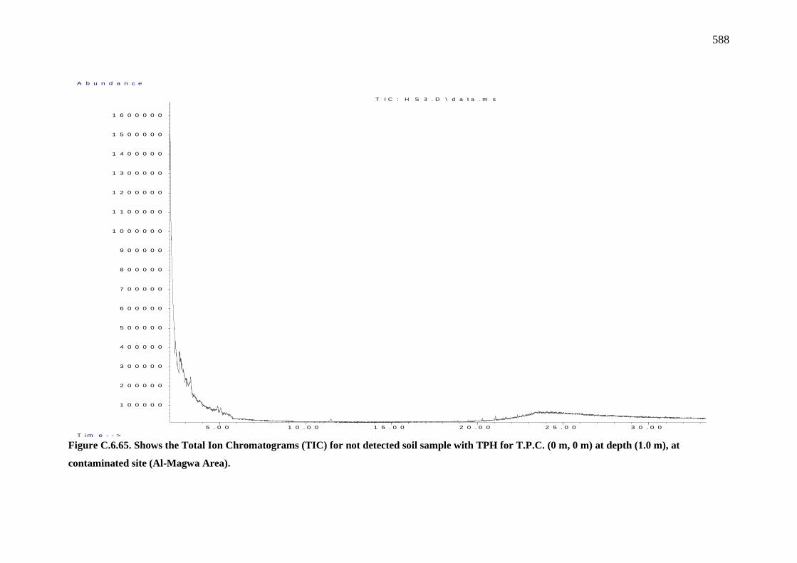
588
Figure C.6.65. Shows the Total Ion Chromatograms (TIC) for not detected soil sample with TPH for T.P.C. (0 m, 0 m) at depth (1.0 m), at
contaminated site (Al-Magwa Area).
5 . 0 0 1 0 . 0 0 1 5 . 0 0 2 0 . 0 0 2 5 . 0 0 3 0 . 0 0
1 0 0 0 0 0
2 0 0 0 0 0
3 0 0 0 0 0
4 0 0 0 0 0
5 0 0 0 0 0
6 0 0 0 0 0
7 0 0 0 0 0
8 0 0 0 0 0
9 0 0 0 0 0
1 0 0 0 0 0 0
1 1 0 0 0 0 0
1 2 0 0 0 0 0
1 3 0 0 0 0 0
1 4 0 0 0 0 0
1 5 0 0 0 0 0
1 6 0 0 0 0 0
T i m e - - >
A b u n d a n c e
T I C : H S 3 . D \ d a t a . m s

589
Figure C.6.66. Shows the Total Ion Chromatograms (TIC) for not detected soil sample with TPH sample for T.P.C. (25 m, 0 m) at depth (1.0 m), at
contaminated site (Al-Magwa Area).
5 . 0 0 1 0 . 0 0 1 5 . 0 0 2 0 . 0 0 2 5 . 0 0 3 0 . 0 0
1 0 0 0 0 0
2 0 0 0 0 0
3 0 0 0 0 0
4 0 0 0 0 0
5 0 0 0 0 0
6 0 0 0 0 0
7 0 0 0 0 0
8 0 0 0 0 0
9 0 0 0 0 0
1 0 0 0 0 0 0
1 1 0 0 0 0 0
1 2 0 0 0 0 0
1 3 0 0 0 0 0
1 4 0 0 0 0 0
1 5 0 0 0 0 0
1 6 0 0 0 0 0
1 7 0 0 0 0 0
1 8 0 0 0 0 0
1 9 0 0 0 0 0
2 0 0 0 0 0 0
2 1 0 0 0 0 0
2 2 0 0 0 0 0
2 3 0 0 0 0 0
2 4 0 0 0 0 0
2 5 0 0 0 0 0
2 6 0 0 0 0 0
2 7 0 0 0 0 0
2 8 0 0 0 0 0
2 9 0 0 0 0 0
3 0 0 0 0 0 0
T i m e - - >
A b u n d a n c e
T I C : H S 1 1 . D \ d a t a . m s
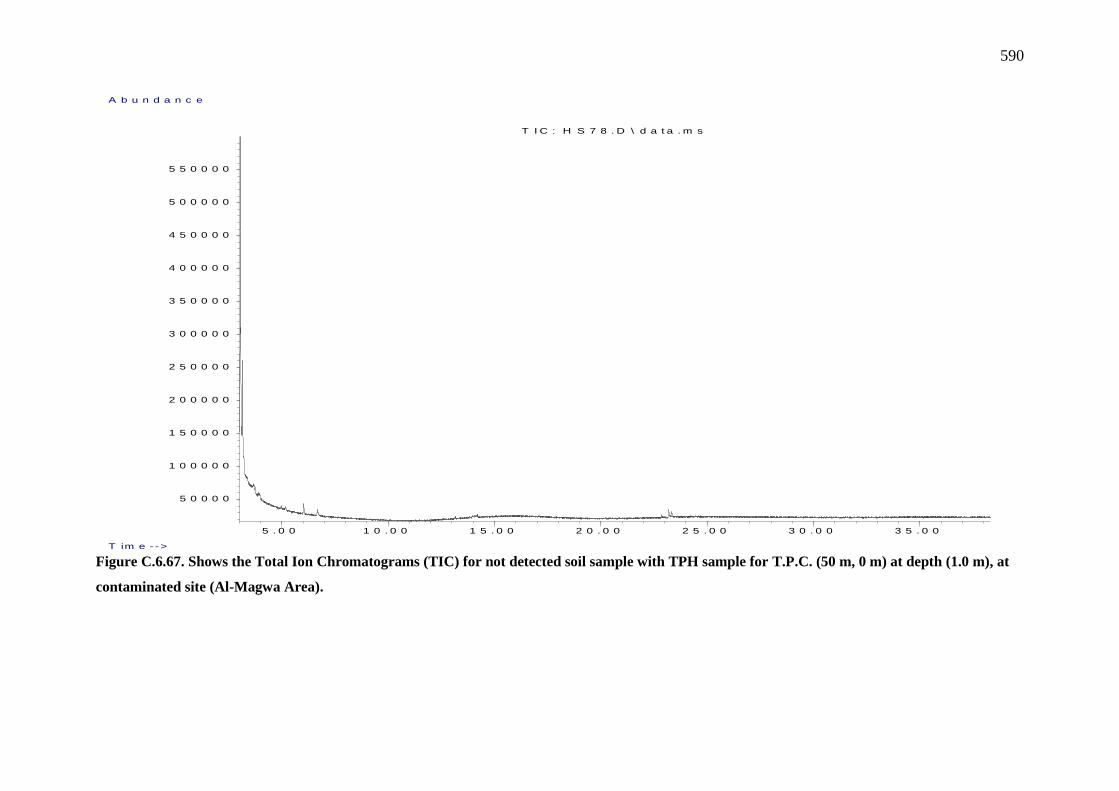
590
Figure C.6.67. Shows the Total Ion Chromatograms (TIC) for not detected soil sample with TPH sample for T.P.C. (50 m, 0 m) at depth (1.0 m), at
contaminated site (Al-Magwa Area).
5 . 0 0 1 0 . 0 0 1 5 . 0 0 2 0 . 0 0 2 5 . 0 0 3 0 . 0 0 3 5 . 0 0
5 0 0 0 0
1 0 0 0 0 0
1 5 0 0 0 0
2 0 0 0 0 0
2 5 0 0 0 0
3 0 0 0 0 0
3 5 0 0 0 0
4 0 0 0 0 0
4 5 0 0 0 0
5 0 0 0 0 0
5 5 0 0 0 0
T im e - - >
A b u n d a n c e
T I C : H S 7 8 . D \ d a t a . m s
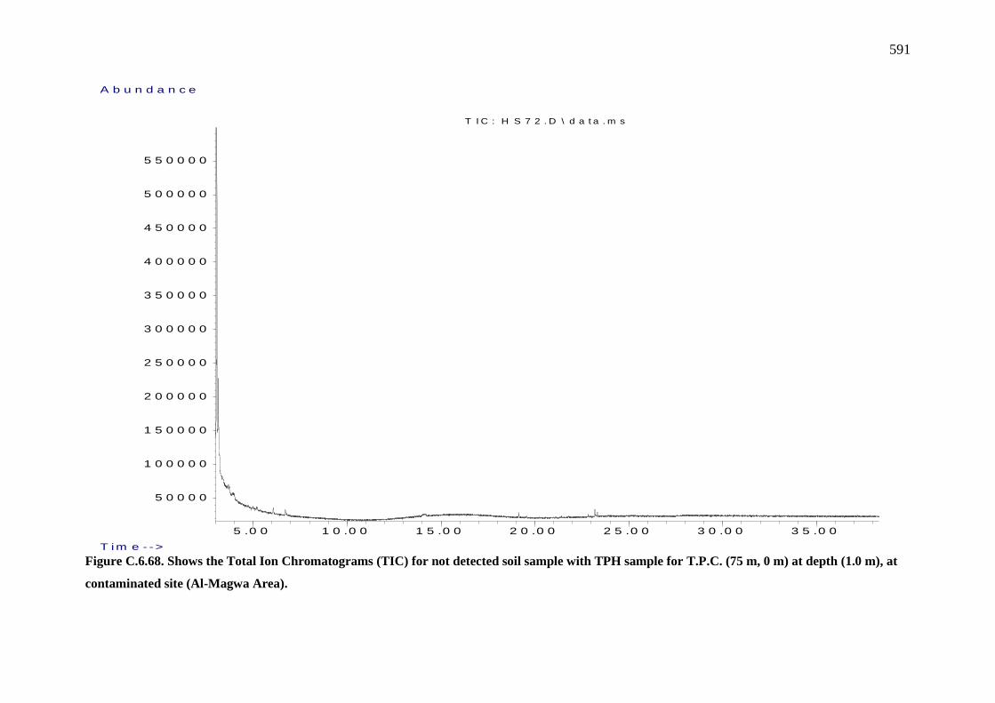
591
Figure C.6.68. Shows the Total Ion Chromatograms (TIC) for not detected soil sample with TPH sample for T.P.C. (75 m, 0 m) at depth (1.0 m), at
contaminated site (Al-Magwa Area).
5 .0 0 1 0 .0 0 1 5 .0 0 2 0 .0 0 2 5 .0 0 3 0 .0 0 3 5 .0 0
5 0 0 0 0
1 0 0 0 0 0
1 5 0 0 0 0
2 0 0 0 0 0
2 5 0 0 0 0
3 0 0 0 0 0
3 5 0 0 0 0
4 0 0 0 0 0
4 5 0 0 0 0
5 0 0 0 0 0
5 5 0 0 0 0
T im e - - >
A b u n d a n c e
T I C : H S 7 2 . D \ d a t a . m s

592
Figure C.6.69. Shows the Total Ion Chromatograms (TIC) for not detected soil sample with TPH sample for T.P.C. (100 m, 0 m) at depth (1.0 m), at
contaminated site (Al-Magwa Area).
5 . 0 0 1 0 . 0 0 1 5 . 0 0 2 0 . 0 0 2 5 . 0 0 3 0 . 0 0 3 5 . 0 0
5 0 0 0 0 0
1 0 0 0 0 0 0
1 5 0 0 0 0 0
2 0 0 0 0 0 0
2 5 0 0 0 0 0
3 0 0 0 0 0 0
3 5 0 0 0 0 0
4 0 0 0 0 0 0
4 5 0 0 0 0 0
5 0 0 0 0 0 0
5 5 0 0 0 0 0
T i m e - - >
A b u n d a n c e
T I C : H S 1 1 6 . D \ d a t a . m s
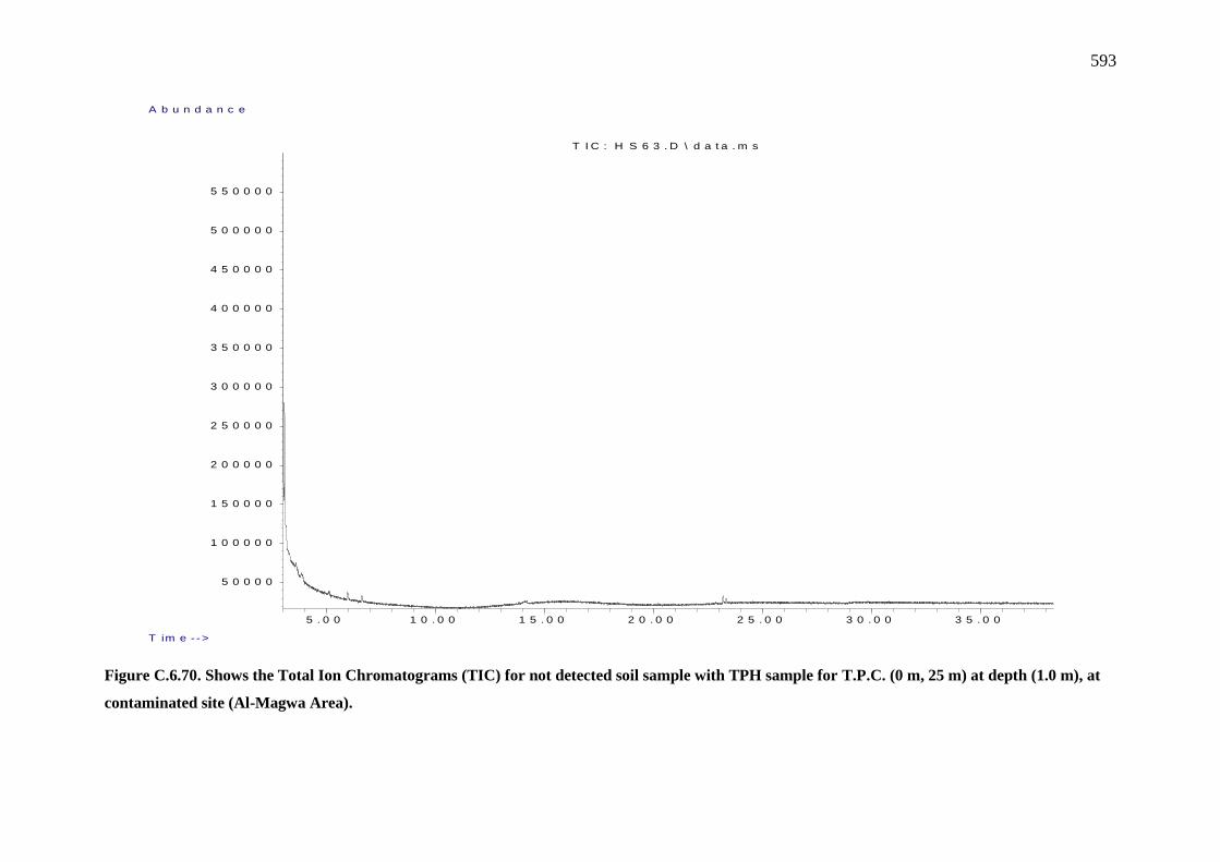
593
Figure C.6.70. Shows the Total Ion Chromatograms (TIC) for not detected soil sample with TPH sample for T.P.C. (0 m, 25 m) at depth (1.0 m), at
contaminated site (Al-Magwa Area).
5 . 0 0 1 0 . 0 0 1 5 . 0 0 2 0 . 0 0 2 5 . 0 0 3 0 . 0 0 3 5 . 0 0
5 0 0 0 0
1 0 0 0 0 0
1 5 0 0 0 0
2 0 0 0 0 0
2 5 0 0 0 0
3 0 0 0 0 0
3 5 0 0 0 0
4 0 0 0 0 0
4 5 0 0 0 0
5 0 0 0 0 0
5 5 0 0 0 0
T im e - - >
A b u n d a n c e
T I C : H S 6 3 . D \ d a t a . m s

594
Figure C.6.71. Shows the Total Ion Chromatograms (TIC) for not detected soil sample with TPH sample for T.P.C. (25 m, 25 m) at depth (1.0 m), at
contaminated site (Al-Magwa Area).
5 . 0 0 1 0 . 0 0 1 5 . 0 0 2 0 . 0 0 2 5 . 0 0 3 0 . 0 0 3 5 . 0 0
5 0 0 0 0 0
1 0 0 0 0 0 0
1 5 0 0 0 0 0
2 0 0 0 0 0 0
2 5 0 0 0 0 0
3 0 0 0 0 0 0
3 5 0 0 0 0 0
4 0 0 0 0 0 0
4 5 0 0 0 0 0
T i m e - - >
A b u n d a n c e
T I C : H S 6 7 . D \ d a t a . m s
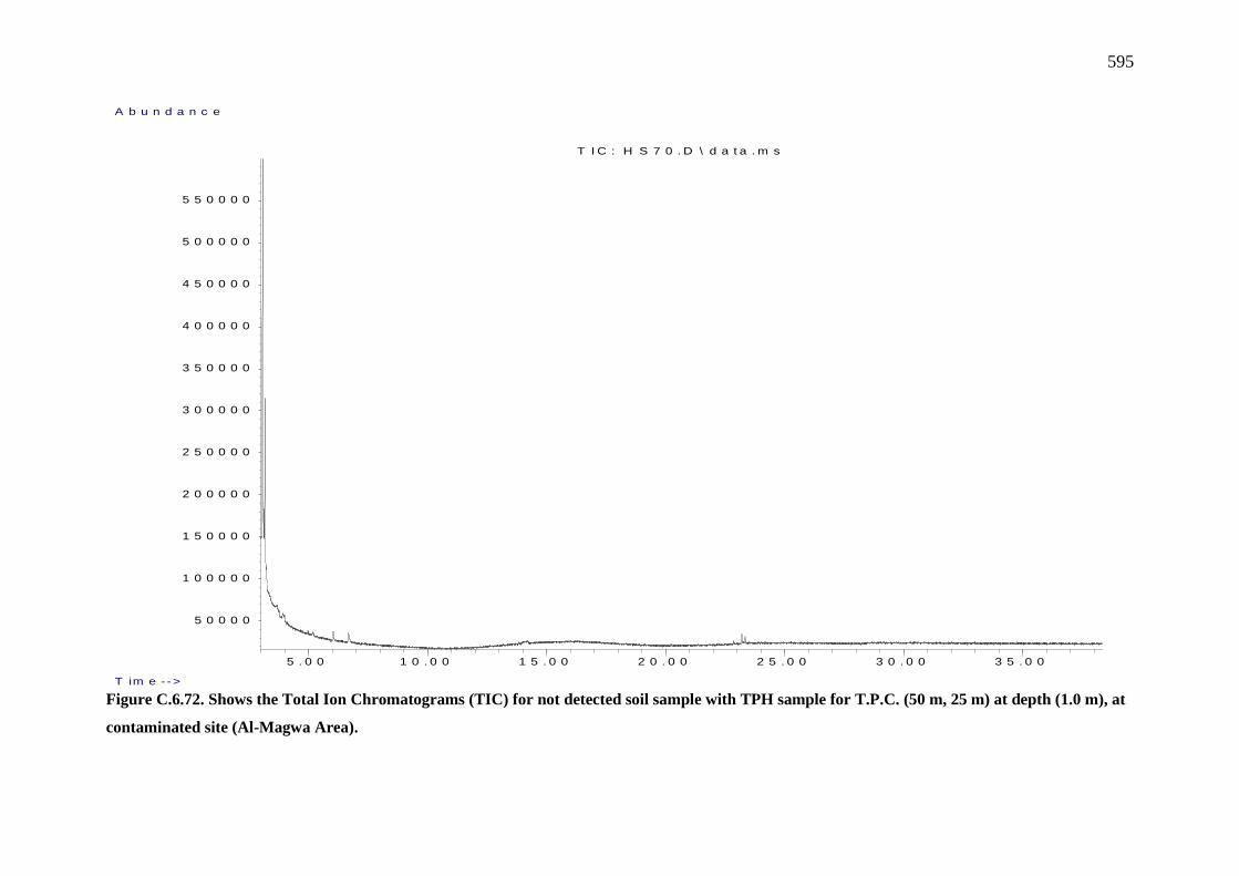
595
Figure C.6.72. Shows the Total Ion Chromatograms (TIC) for not detected soil sample with TPH sample for T.P.C. (50 m, 25 m) at depth (1.0 m), at
contaminated site (Al-Magwa Area).
5 . 0 0 1 0 . 0 0 1 5 . 0 0 2 0 . 0 0 2 5 . 0 0 3 0 . 0 0 3 5 . 0 0
5 0 0 0 0
1 0 0 0 0 0
1 5 0 0 0 0
2 0 0 0 0 0
2 5 0 0 0 0
3 0 0 0 0 0
3 5 0 0 0 0
4 0 0 0 0 0
4 5 0 0 0 0
5 0 0 0 0 0
5 5 0 0 0 0
T im e - - >
A b u n d a n c e
T I C : H S 7 0 . D \ d a t a . m s
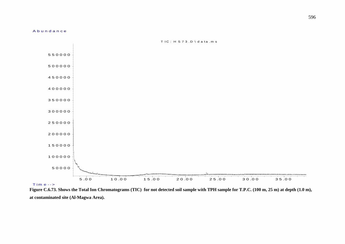
596
Figure C.6.73. Shows the Total Ion Chromatograms (TIC) for not detected soil sample with TPH sample for T.P.C. (100 m, 25 m) at depth (1.0 m),
at contaminated site (Al-Magwa Area).
5 .0 0 1 0 .0 0 1 5 .0 0 2 0 .0 0 2 5 .0 0 3 0 .0 0 3 5 .0 0
5 0 0 0 0
1 0 0 0 0 0
1 5 0 0 0 0
2 0 0 0 0 0
2 5 0 0 0 0
3 0 0 0 0 0
3 5 0 0 0 0
4 0 0 0 0 0
4 5 0 0 0 0
5 0 0 0 0 0
5 5 0 0 0 0
T im e - - >
A b u n d a n c e
T I C : H S 7 3 . D \ d a t a . m s
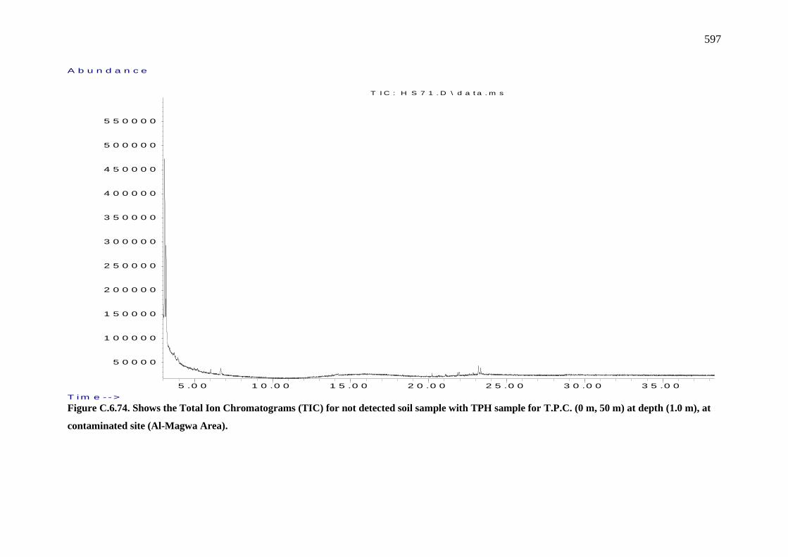
597
Figure C.6.74. Shows the Total Ion Chromatograms (TIC) for not detected soil sample with TPH sample for T.P.C. (0 m, 50 m) at depth (1.0 m), at
contaminated site (Al-Magwa Area).
5 .0 0 1 0 .0 0 1 5 .0 0 2 0 .0 0 2 5 .0 0 3 0 .0 0 3 5 .0 0
5 0 0 0 0
1 0 0 0 0 0
1 5 0 0 0 0
2 0 0 0 0 0
2 5 0 0 0 0
3 0 0 0 0 0
3 5 0 0 0 0
4 0 0 0 0 0
4 5 0 0 0 0
5 0 0 0 0 0
5 5 0 0 0 0
T im e - - >
A b u n d a n c e
T I C : H S 7 1 . D \ d a t a . m s
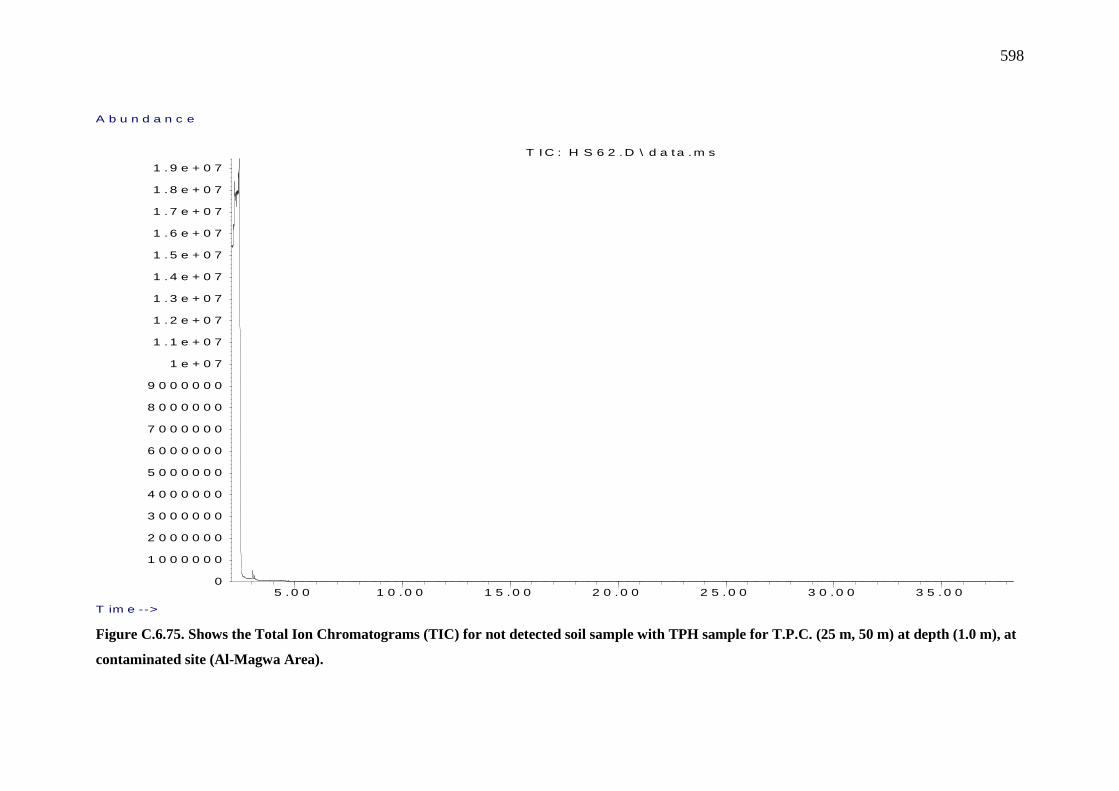
598
Figure C.6.75. Shows the Total Ion Chromatograms (TIC) for not detected soil sample with TPH sample for T.P.C. (25 m, 50 m) at depth (1.0 m), at
contaminated site (Al-Magwa Area).
5 .0 0 1 0 . 0 0 1 5 . 0 0 2 0 . 0 0 2 5 . 0 0 3 0 . 0 0 3 5 . 0 00
1 0 0 0 0 0 0
2 0 0 0 0 0 0
3 0 0 0 0 0 0
4 0 0 0 0 0 0
5 0 0 0 0 0 0
6 0 0 0 0 0 0
7 0 0 0 0 0 0
8 0 0 0 0 0 0
9 0 0 0 0 0 0
1 e + 0 7
1 . 1 e + 0 7
1 . 2 e + 0 7
1 . 3 e + 0 7
1 . 4 e + 0 7
1 . 5 e + 0 7
1 . 6 e + 0 7
1 . 7 e + 0 7
1 . 8 e + 0 7
1 . 9 e + 0 7
T im e -->
A b u n d a n c e
T I C : H S 6 2 .D \ d a ta . m s
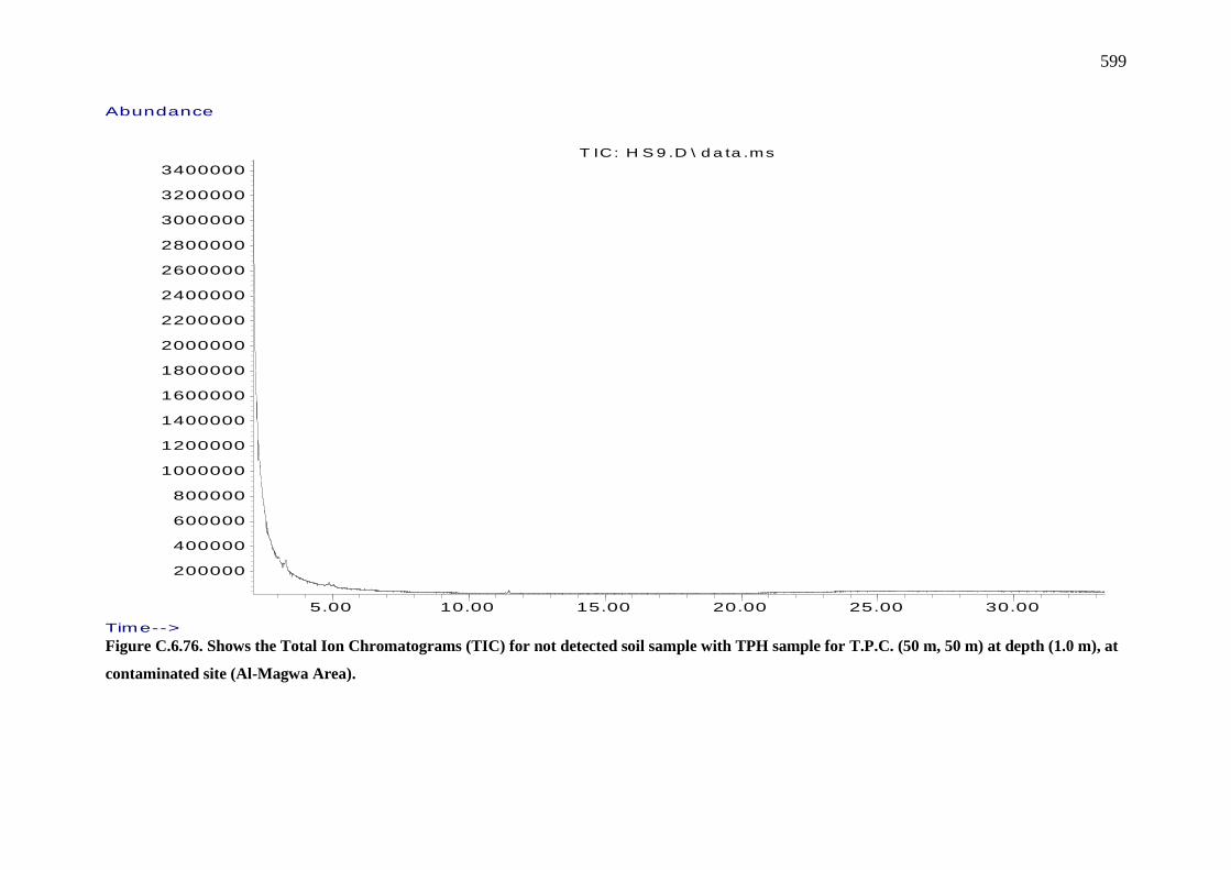
599
Figure C.6.76. Shows the Total Ion Chromatograms (TIC) for not detected soil sample with TPH sample for T.P.C. (50 m, 50 m) at depth (1.0 m), at
contaminated site (Al-Magwa Area).
5.00 10.00 15.00 20.00 25.00 30.00
200000
400000
600000
800000
1000000
1200000
1400000
1600000
1800000
2000000
2200000
2400000
2600000
2800000
3000000
3200000
3400000
Time-->
Abundance
T IC: H S 9 .D \ d a ta .ms

600
Figure C.6.77. Shows the Total Ion Chromatograms (TIC) for not detected soil sample with TPH sample for T.P.C. (100 m, 50 m) at depth (1.0 m), at
contaminated site (Al-Magwa Area).
5 . 0 0 1 0 . 0 0 1 5 . 0 0 2 0 . 0 0 2 5 . 0 0 3 0 . 0 0 3 5 . 0 0
5 0 0 0 0
1 0 0 0 0 0
1 5 0 0 0 0
2 0 0 0 0 0
2 5 0 0 0 0
3 0 0 0 0 0
3 5 0 0 0 0
4 0 0 0 0 0
4 5 0 0 0 0
5 0 0 0 0 0
5 5 0 0 0 0
T im e - - >
A b u n d a n c e
T I C : H S 7 7 . D \ d a t a . m s
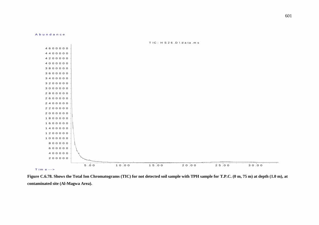
601
Figure C.6.78. Shows the Total Ion Chromatograms (TIC) for not detected soil sample with TPH sample for T.P.C. (0 m, 75 m) at depth (1.0 m), at
contaminated site (Al-Magwa Area).
5 .0 0 1 0 .0 0 1 5 .0 0 2 0 .0 0 2 5 .0 0 3 0 .0 0
2 0 0 0 0 0
4 0 0 0 0 0
6 0 0 0 0 0
8 0 0 0 0 0
1 0 0 0 0 0 0
1 2 0 0 0 0 0
1 4 0 0 0 0 0
1 6 0 0 0 0 0
1 8 0 0 0 0 0
2 0 0 0 0 0 0
2 2 0 0 0 0 0
2 4 0 0 0 0 0
2 6 0 0 0 0 0
2 8 0 0 0 0 0
3 0 0 0 0 0 0
3 2 0 0 0 0 0
3 4 0 0 0 0 0
3 6 0 0 0 0 0
3 8 0 0 0 0 0
4 0 0 0 0 0 0
4 2 0 0 0 0 0
4 4 0 0 0 0 0
4 6 0 0 0 0 0
T i m e - - >
A b u n d a n c e
T I C : H S 2 6 . D \ d a t a . m s
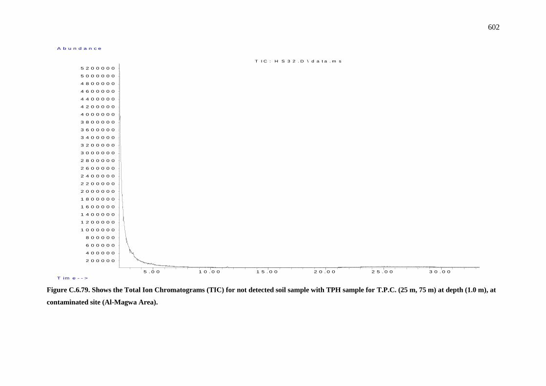
602
Figure C.6.79. Shows the Total Ion Chromatograms (TIC) for not detected soil sample with TPH sample for T.P.C. (25 m, 75 m) at depth (1.0 m), at
contaminated site (Al-Magwa Area).
5 . 0 0 1 0 . 0 0 1 5 . 0 0 2 0 . 0 0 2 5 . 0 0 3 0 . 0 0
2 0 0 0 0 0
4 0 0 0 0 0
6 0 0 0 0 0
8 0 0 0 0 0
1 0 0 0 0 0 0
1 2 0 0 0 0 0
1 4 0 0 0 0 0
1 6 0 0 0 0 0
1 8 0 0 0 0 0
2 0 0 0 0 0 0
2 2 0 0 0 0 0
2 4 0 0 0 0 0
2 6 0 0 0 0 0
2 8 0 0 0 0 0
3 0 0 0 0 0 0
3 2 0 0 0 0 0
3 4 0 0 0 0 0
3 6 0 0 0 0 0
3 8 0 0 0 0 0
4 0 0 0 0 0 0
4 2 0 0 0 0 0
4 4 0 0 0 0 0
4 6 0 0 0 0 0
4 8 0 0 0 0 0
5 0 0 0 0 0 0
5 2 0 0 0 0 0
T im e - - >
A b u n d a n c e
T I C : H S 3 2 . D \ d a t a . m s
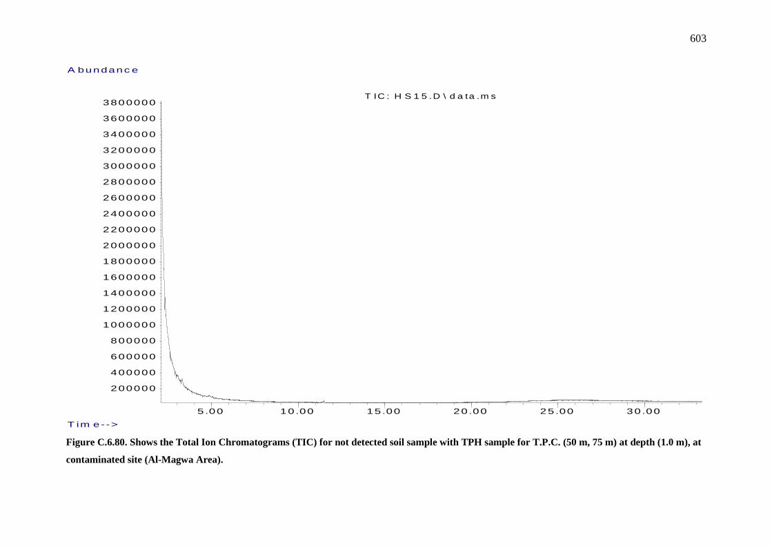
603
Figure C.6.80. Shows the Total Ion Chromatograms (TIC) for not detected soil sample with TPH sample for T.P.C. (50 m, 75 m) at depth (1.0 m), at
contaminated site (Al-Magwa Area).
5.00 10.00 15.00 20.00 25.00 30.00
200000
400000
600000
800000
1000000
1200000
1400000
1600000
1800000
2000000
2200000
2400000
2600000
2800000
3000000
3200000
3400000
3600000
3800000
T im e-->
A bundanc e
T IC : H S 1 5 .D \ d a ta .m s

604
Figure C.6.81. Shows the Total Ion Chromatograms (TIC) for not detected soil sample with TPH sample for T.P.C. (75 m, 75 m) at depth (1.0 m), at
contaminated site (Al-Magwa Area).
5 . 0 0 1 0 . 0 0 1 5 . 0 0 2 0 . 0 0 2 5 . 0 0 3 0 . 0 0
2 0 0 0 0 0
4 0 0 0 0 0
6 0 0 0 0 0
8 0 0 0 0 0
1 0 0 0 0 0 0
1 2 0 0 0 0 0
1 4 0 0 0 0 0
1 6 0 0 0 0 0
1 8 0 0 0 0 0
2 0 0 0 0 0 0
2 2 0 0 0 0 0
2 4 0 0 0 0 0
2 6 0 0 0 0 0
2 8 0 0 0 0 0
3 0 0 0 0 0 0
3 2 0 0 0 0 0
3 4 0 0 0 0 0
3 6 0 0 0 0 0
3 8 0 0 0 0 0
4 0 0 0 0 0 0
4 2 0 0 0 0 0
4 4 0 0 0 0 0
4 6 0 0 0 0 0
4 8 0 0 0 0 0
5 0 0 0 0 0 0
T i m e - - >
A b u n d a n c e
T I C : H S 4 0 . D \ d a t a . m s
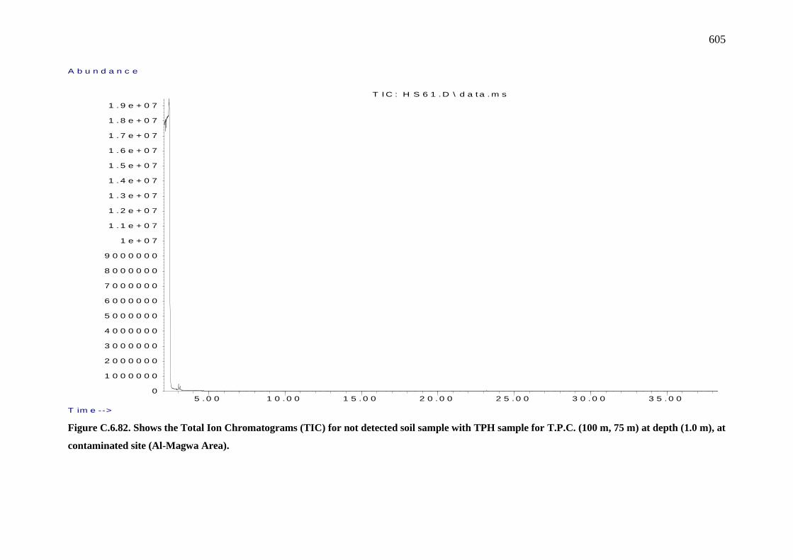
605
Figure C.6.82. Shows the Total Ion Chromatograms (TIC) for not detected soil sample with TPH sample for T.P.C. (100 m, 75 m) at depth (1.0 m), at
contaminated site (Al-Magwa Area).
5 .0 0 1 0 . 0 0 1 5 . 0 0 2 0 . 0 0 2 5 . 0 0 3 0 . 0 0 3 5 . 0 00
1 0 0 0 0 0 0
2 0 0 0 0 0 0
3 0 0 0 0 0 0
4 0 0 0 0 0 0
5 0 0 0 0 0 0
6 0 0 0 0 0 0
7 0 0 0 0 0 0
8 0 0 0 0 0 0
9 0 0 0 0 0 0
1 e + 0 7
1 . 1 e + 0 7
1 . 2 e + 0 7
1 . 3 e + 0 7
1 . 4 e + 0 7
1 . 5 e + 0 7
1 . 6 e + 0 7
1 . 7 e + 0 7
1 . 8 e + 0 7
1 . 9 e + 0 7
T im e -->
A b u n d a n c e
T I C : H S 6 1 .D \ d a ta . m s
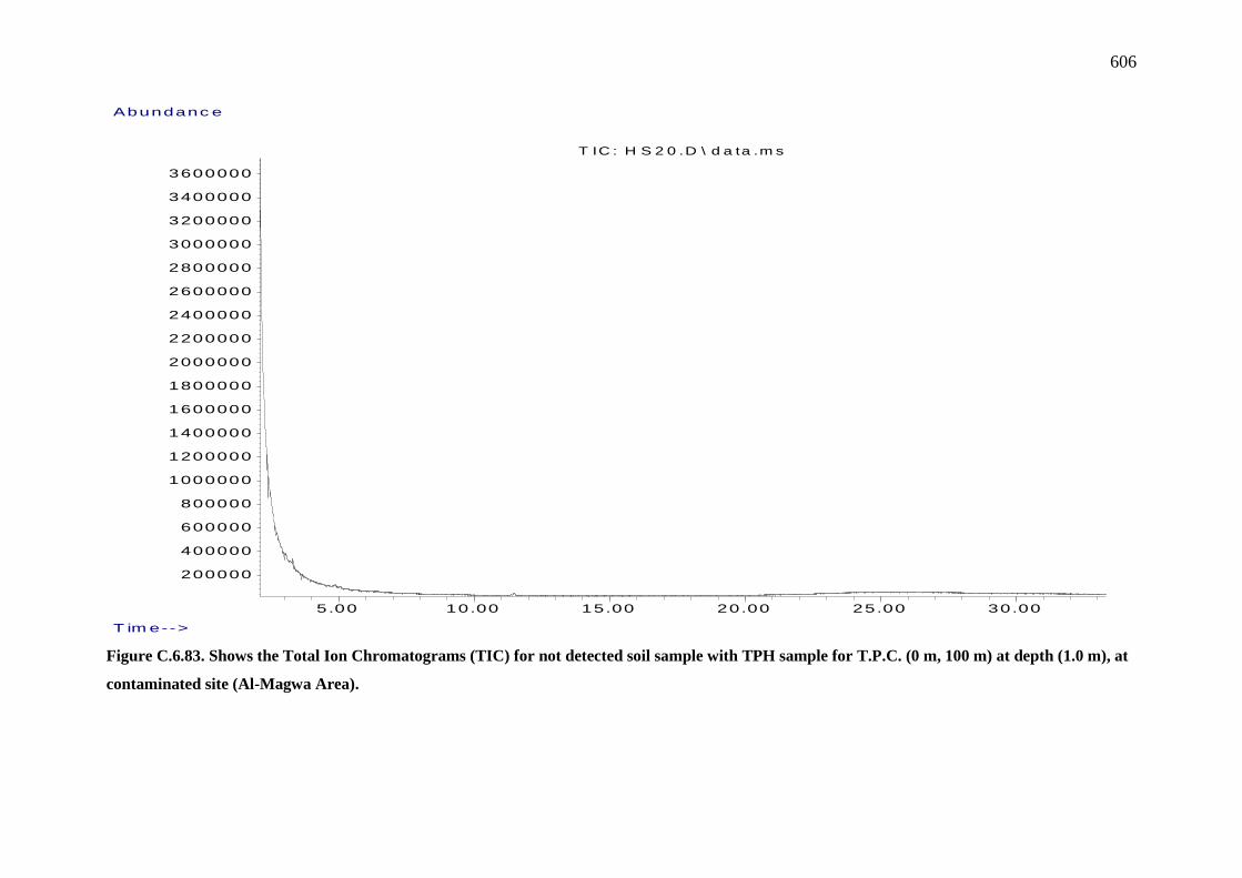
606
Figure C.6.83. Shows the Total Ion Chromatograms (TIC) for not detected soil sample with TPH sample for T.P.C. (0 m, 100 m) at depth (1.0 m), at
contaminated site (Al-Magwa Area).
5.00 10.00 15.00 20.00 25.00 30.00
200000
400000
600000
800000
1000000
1200000
1400000
1600000
1800000
2000000
2200000
2400000
2600000
2800000
3000000
3200000
3400000
3600000
T im e-->
Abundanc e
T IC : H S 2 0 .D \ d a ta .m s

607
Figure C.6.84. Shows the Total Ion Chromatograms (TIC) for not detected soil sample with TPH sample for T.P.C. (50 m, 100 m) at depth (1.0 m),
at contaminated site (Al-Magwa Area).
5 . 0 0 1 0 . 0 0 1 5 . 0 0 2 0 . 0 0 2 5 . 0 0 3 0 . 0 0 3 5 . 0 0
5 0 0 0 0
1 0 0 0 0 0
1 5 0 0 0 0
2 0 0 0 0 0
2 5 0 0 0 0
3 0 0 0 0 0
3 5 0 0 0 0
4 0 0 0 0 0
4 5 0 0 0 0
5 0 0 0 0 0
5 5 0 0 0 0
T im e - - >
A b u n d a n c e
T I C : H S 6 9 . D \ d a t a . m s

608
Figure C.6.85. Shows the Total Ion Chromatograms (TIC) for not detected soil sample with TPH sample for T.P.C. (75 m, 100 m) at depth (1.0 m), at
contaminated site (Al-Magwa Area).
5 . 0 0 1 0 . 0 0 1 5 . 0 0 2 0 . 0 0 2 5 . 0 0 3 0 . 0 0 3 5 . 0 0
5 0 0 0 0
1 0 0 0 0 0
1 5 0 0 0 0
2 0 0 0 0 0
2 5 0 0 0 0
3 0 0 0 0 0
3 5 0 0 0 0
4 0 0 0 0 0
4 5 0 0 0 0
5 0 0 0 0 0
5 5 0 0 0 0
T im e - - >
A b u n d a n c e
T I C : H S 6 8 . D \ d a t a . m s
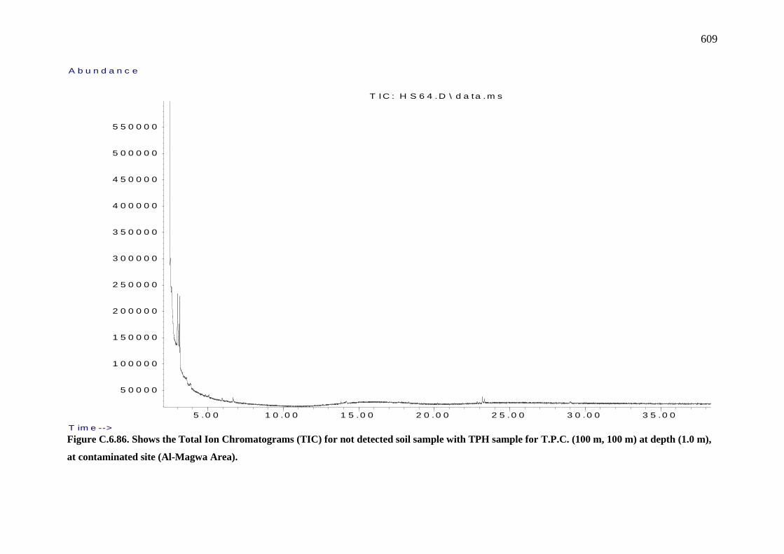
609
Figure C.6.86. Shows the Total Ion Chromatograms (TIC) for not detected soil sample with TPH sample for T.P.C. (100 m, 100 m) at depth (1.0 m),
at contaminated site (Al-Magwa Area).
5 .0 0 1 0 .0 0 1 5 .0 0 2 0 .0 0 2 5 .0 0 3 0 .0 0 3 5 .0 0
5 0 0 0 0
1 0 0 0 0 0
1 5 0 0 0 0
2 0 0 0 0 0
2 5 0 0 0 0
3 0 0 0 0 0
3 5 0 0 0 0
4 0 0 0 0 0
4 5 0 0 0 0
5 0 0 0 0 0
5 5 0 0 0 0
T im e -->
A b u n d a n c e
T IC : H S 6 4 .D \ d a ta .m s

610
At Depth (1.5 m)
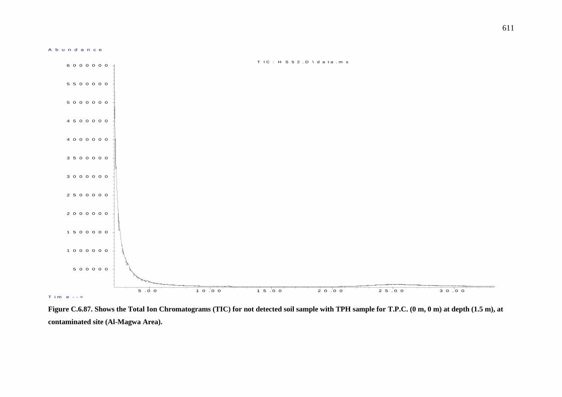
611
Figure C.6.87. Shows the Total Ion Chromatograms (TIC) for not detected soil sample with TPH sample for T.P.C. (0 m, 0 m) at depth (1.5 m), at
contaminated site (Al-Magwa Area).
5 . 0 0 1 0 . 0 0 1 5 . 0 0 2 0 . 0 0 2 5 . 0 0 3 0 . 0 0
5 0 0 0 0 0
1 0 0 0 0 0 0
1 5 0 0 0 0 0
2 0 0 0 0 0 0
2 5 0 0 0 0 0
3 0 0 0 0 0 0
3 5 0 0 0 0 0
4 0 0 0 0 0 0
4 5 0 0 0 0 0
5 0 0 0 0 0 0
5 5 0 0 0 0 0
6 0 0 0 0 0 0
T i m e - - >
A b u n d a n c e
T I C : H S 5 2 . D \ d a t a . m s

612
Figure C.6.88. Shows the Total Ion Chromatograms (TIC) for not detected soil sample with TPH sample for T.P.C. (25 m, 0 m) at depth (1.5 m), at
contaminated site (Al-Magwa Area).
5 . 0 0 1 0 . 0 0 1 5 . 0 0 2 0 . 0 0 2 5 . 0 0 3 0 . 0 0 3 5 . 0 0
5 0 0 0 0 0
1 0 0 0 0 0 0
1 5 0 0 0 0 0
2 0 0 0 0 0 0
2 5 0 0 0 0 0
3 0 0 0 0 0 0
3 5 0 0 0 0 0
4 0 0 0 0 0 0
4 5 0 0 0 0 0
5 0 0 0 0 0 0
5 5 0 0 0 0 0
T i m e - - >
A b u n d a n c e
T I C : H S 1 1 7 . D \ d a t a . m s
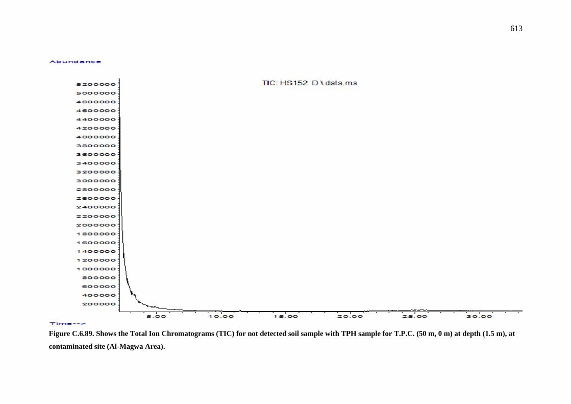
613
Figure C.6.89. Shows the Total Ion Chromatograms (TIC) for not detected soil sample with TPH sample for T.P.C. (50 m, 0 m) at depth (1.5 m), at
contaminated site (Al-Magwa Area).

614
Figure C.6.90. Shows the Total Ion Chromatograms (TIC) for not detected soil sample with TPH sample for T.P.C. (75 m, 0 m) at depth (1.5 m), at
contaminated site (Al-Magwa Area).
5 .0 0 1 0 .0 0 1 5 .0 0 2 0 .0 0 2 5 .0 0 3 0 .0 0
2 0 0 0 0 0
4 0 0 0 0 0
6 0 0 0 0 0
8 0 0 0 0 0
1 0 0 0 0 0 0
1 2 0 0 0 0 0
1 4 0 0 0 0 0
1 6 0 0 0 0 0
1 8 0 0 0 0 0
2 0 0 0 0 0 0
2 2 0 0 0 0 0
2 4 0 0 0 0 0
2 6 0 0 0 0 0
2 8 0 0 0 0 0
3 0 0 0 0 0 0
3 2 0 0 0 0 0
3 4 0 0 0 0 0
3 6 0 0 0 0 0
3 8 0 0 0 0 0
4 0 0 0 0 0 0
4 2 0 0 0 0 0
T i m e - - >
A b u n d a n c e
T I C : H S 3 3 . D \ d a t a . m s
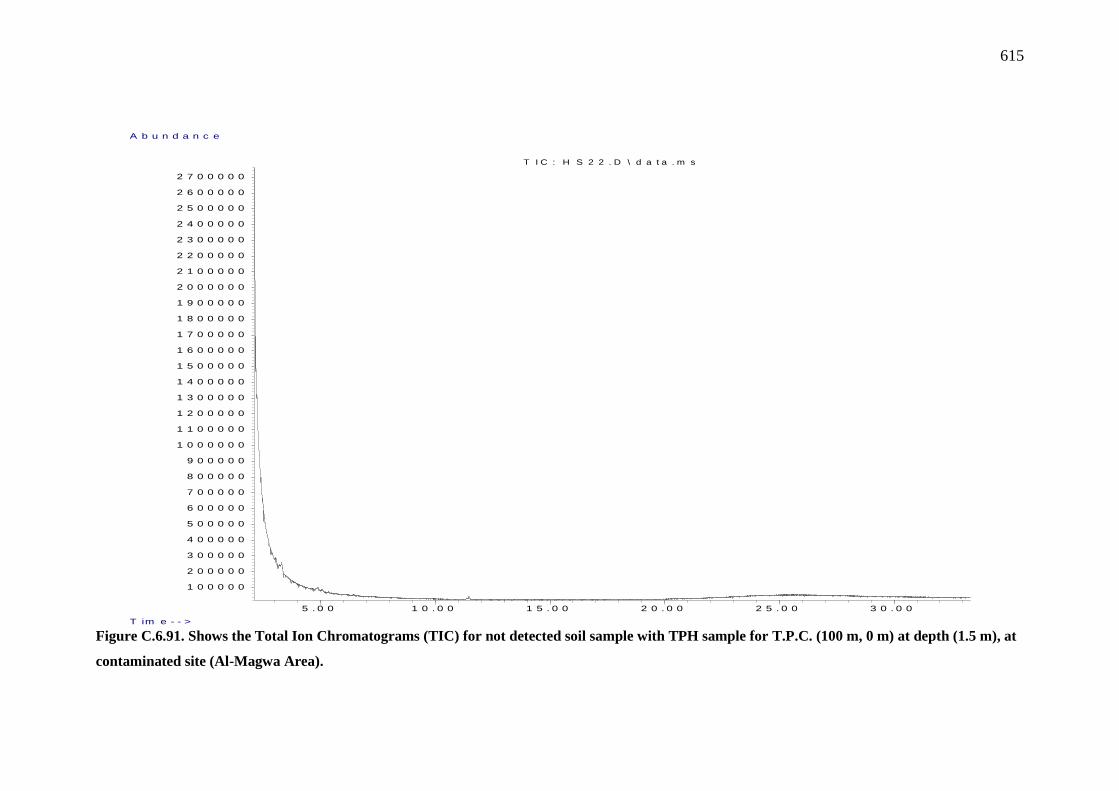
615
Figure C.6.91. Shows the Total Ion Chromatograms (TIC) for not detected soil sample with TPH sample for T.P.C. (100 m, 0 m) at depth (1.5 m), at
contaminated site (Al-Magwa Area).
5 . 0 0 1 0 . 0 0 1 5 . 0 0 2 0 . 0 0 2 5 . 0 0 3 0 . 0 0
1 0 0 0 0 0
2 0 0 0 0 0
3 0 0 0 0 0
4 0 0 0 0 0
5 0 0 0 0 0
6 0 0 0 0 0
7 0 0 0 0 0
8 0 0 0 0 0
9 0 0 0 0 0
1 0 0 0 0 0 0
1 1 0 0 0 0 0
1 2 0 0 0 0 0
1 3 0 0 0 0 0
1 4 0 0 0 0 0
1 5 0 0 0 0 0
1 6 0 0 0 0 0
1 7 0 0 0 0 0
1 8 0 0 0 0 0
1 9 0 0 0 0 0
2 0 0 0 0 0 0
2 1 0 0 0 0 0
2 2 0 0 0 0 0
2 3 0 0 0 0 0
2 4 0 0 0 0 0
2 5 0 0 0 0 0
2 6 0 0 0 0 0
2 7 0 0 0 0 0
T im e - - >
A b u n d a n c e
T I C : H S 2 2 . D \ d a t a . m s

616
Figure C.6.92. Shows the Total Ion Chromatograms (TIC) for not detected soil sample with TPH sample for T.P.C. (0 m, 25 m) at depth (1.5 m), at
contaminated site (Al-Magwa Area).
5 . 0 0 1 0 . 0 0 1 5 . 0 0 2 0 . 0 0 2 5 . 0 0 3 0 . 0 0 3 5 . 0 0
5 0 0 0 0 0
1 0 0 0 0 0 0
1 5 0 0 0 0 0
2 0 0 0 0 0 0
2 5 0 0 0 0 0
3 0 0 0 0 0 0
3 5 0 0 0 0 0
4 0 0 0 0 0 0
4 5 0 0 0 0 0
5 0 0 0 0 0 0
5 5 0 0 0 0 0
T i m e - - >
A b u n d a n c e
T I C : H S 6 0 a . D \ d a t a . m s

617
Figure C.6.93. Shows the Total Ion Chromatograms (TIC) for not detected soil sample with TPH sample for T.P.C. (25 m, 25 m) at depth
(1.5 m), at contaminated site (Al-Magwa Area).
5 . 0 0 1 0 . 0 0 1 5 . 0 0 2 0 . 0 0 2 5 . 0 0 3 0 . 0 0 3 5 . 0 0
5 0 0 0 0 0
1 0 0 0 0 0 0
1 5 0 0 0 0 0
2 0 0 0 0 0 0
2 5 0 0 0 0 0
3 0 0 0 0 0 0
3 5 0 0 0 0 0
4 0 0 0 0 0 0
4 5 0 0 0 0 0
5 0 0 0 0 0 0
5 5 0 0 0 0 0
T i m e - - >
A b u n d a n c e
T I C : H S 1 1 0 . D \ d a t a . m s
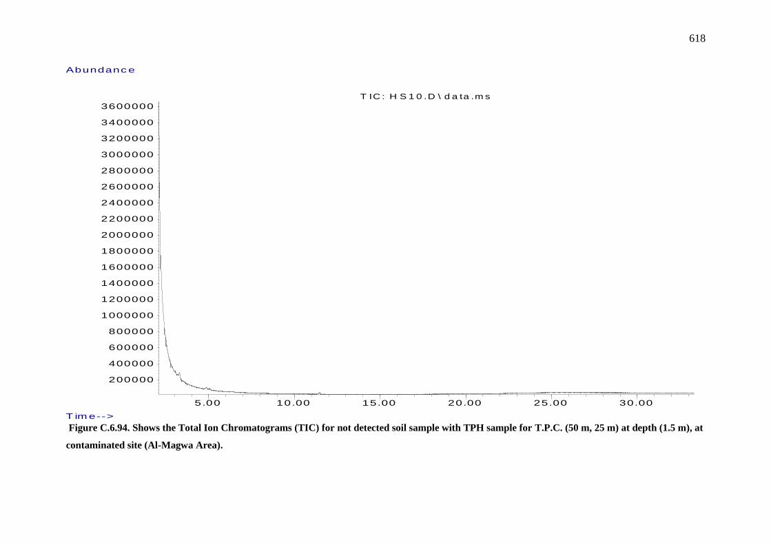
618
Figure C.6.94. Shows the Total Ion Chromatograms (TIC) for not detected soil sample with TPH sample for T.P.C. (50 m, 25 m) at depth (1.5 m), at
contaminated site (Al-Magwa Area).
5.00 10.00 15.00 20.00 25.00 30.00
200000
400000
600000
800000
1000000
1200000
1400000
1600000
1800000
2000000
2200000
2400000
2600000
2800000
3000000
3200000
3400000
3600000
T im e-->
Abundanc e
T IC : H S 1 0 .D \ d a ta .m s

619
Figure C.6.95. Shows the Total Ion Chromatograms (TIC) for not detected soil sample with TPH sample for T.P.C. (100 m, 25 m) at depth (1.5 m), at
contaminated site (Al-Magwa Area).
5 . 0 0 1 0 . 0 0 1 5 . 0 0 2 0 . 0 0 2 5 . 0 0 3 0 . 0 0 3 5 . 0 0
5 0 0 0 0 0
1 0 0 0 0 0 0
1 5 0 0 0 0 0
2 0 0 0 0 0 0
2 5 0 0 0 0 0
3 0 0 0 0 0 0
3 5 0 0 0 0 0
4 0 0 0 0 0 0
4 5 0 0 0 0 0
5 0 0 0 0 0 0
5 5 0 0 0 0 0
T i m e - - >
A b u n d a n c e
T I C : H S 1 1 8 . D \ d a t a . m s

620
Figure C.6.96. Shows the Total Ion Chromatograms (TIC) for not detected soil sample with TPH sample for T.P.C. (0 m, 50 m) at depth (1.5 m), at
contaminated site (Al-Magwa Area).
5 . 0 0 1 0 . 0 0 1 5 . 0 0 2 0 . 0 0 2 5 . 0 0 3 0 . 0 0
2 0 0 0 0 0
4 0 0 0 0 0
6 0 0 0 0 0
8 0 0 0 0 0
1 0 0 0 0 0 0
1 2 0 0 0 0 0
1 4 0 0 0 0 0
1 6 0 0 0 0 0
1 8 0 0 0 0 0
2 0 0 0 0 0 0
2 2 0 0 0 0 0
2 4 0 0 0 0 0
2 6 0 0 0 0 0
2 8 0 0 0 0 0
3 0 0 0 0 0 0
3 2 0 0 0 0 0
3 4 0 0 0 0 0
3 6 0 0 0 0 0
3 8 0 0 0 0 0
4 0 0 0 0 0 0
4 2 0 0 0 0 0
4 4 0 0 0 0 0
4 6 0 0 0 0 0
4 8 0 0 0 0 0
5 0 0 0 0 0 0
5 2 0 0 0 0 0
T i m e - - >
A b u n d a n c e
T I C : H S 1 2 . D \ d a t a . m s
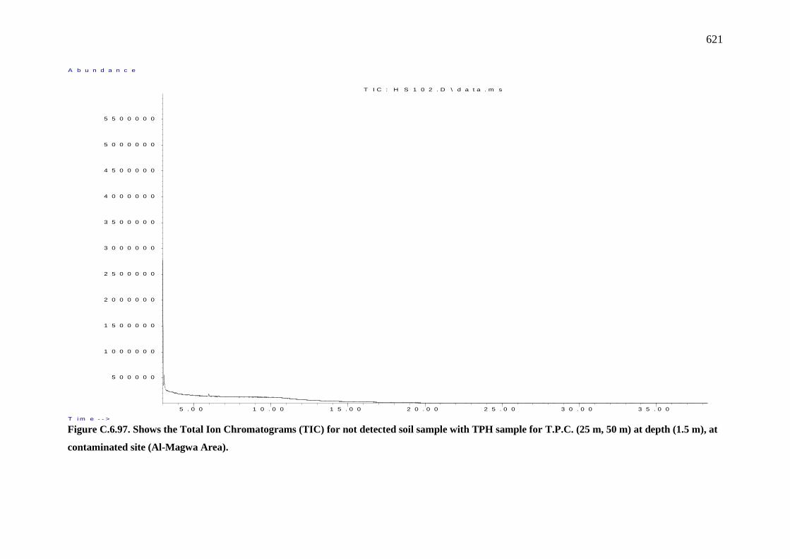
621
Figure C.6.97. Shows the Total Ion Chromatograms (TIC) for not detected soil sample with TPH sample for T.P.C. (25 m, 50 m) at depth (1.5 m), at
contaminated site (Al-Magwa Area).
5 . 0 0 1 0 . 0 0 1 5 . 0 0 2 0 . 0 0 2 5 . 0 0 3 0 . 0 0 3 5 . 0 0
5 0 0 0 0 0
1 0 0 0 0 0 0
1 5 0 0 0 0 0
2 0 0 0 0 0 0
2 5 0 0 0 0 0
3 0 0 0 0 0 0
3 5 0 0 0 0 0
4 0 0 0 0 0 0
4 5 0 0 0 0 0
5 0 0 0 0 0 0
5 5 0 0 0 0 0
T i m e - - >
A b u n d a n c e
T I C : H S 1 0 2 . D \ d a t a . m s

622
Figure C.6.98. Shows the Total Ion Chromatograms (TIC) for not detected soil sample with TPH sample for T.P.C. (50 m, 50 m) at depth (1.5 m), at
contaminated site (Al-Magwa Area).
5 . 0 0 1 0 . 0 0 1 5 . 0 0 2 0 . 0 0 2 5 . 0 0 3 0 . 0 0
1 0 0 0 0 0
2 0 0 0 0 0
3 0 0 0 0 0
4 0 0 0 0 0
5 0 0 0 0 0
6 0 0 0 0 0
7 0 0 0 0 0
8 0 0 0 0 0
9 0 0 0 0 0
1 0 0 0 0 0 0
1 1 0 0 0 0 0
1 2 0 0 0 0 0
1 3 0 0 0 0 0
1 4 0 0 0 0 0
1 5 0 0 0 0 0
1 6 0 0 0 0 0
1 7 0 0 0 0 0
1 8 0 0 0 0 0
1 9 0 0 0 0 0
2 0 0 0 0 0 0
2 1 0 0 0 0 0
2 2 0 0 0 0 0
2 3 0 0 0 0 0
2 4 0 0 0 0 0
2 5 0 0 0 0 0
2 6 0 0 0 0 0
2 7 0 0 0 0 0
2 8 0 0 0 0 0
2 9 0 0 0 0 0
3 0 0 0 0 0 0
T i m e - - >
A b u n d a n c e
T I C : H S 1 6 . D \ d a t a . m s

623
Figure C.6.99. Shows the Total Ion Chromatograms (TIC) for not detected soil sample with TPH sample for T.P.C. (100 m, 50 m) at depth (1.5 m), at
contaminated site (Al-Magwa Area).
5 .0 0 1 0 .0 0 1 5 .0 0 2 0 .0 0 2 5 .0 0 3 0 .0 0
2 0 0 0 0 0
4 0 0 0 0 0
6 0 0 0 0 0
8 0 0 0 0 0
1 0 0 0 0 0 0
1 2 0 0 0 0 0
1 4 0 0 0 0 0
1 6 0 0 0 0 0
1 8 0 0 0 0 0
2 0 0 0 0 0 0
2 2 0 0 0 0 0
2 4 0 0 0 0 0
2 6 0 0 0 0 0
2 8 0 0 0 0 0
3 0 0 0 0 0 0
3 2 0 0 0 0 0
3 4 0 0 0 0 0
3 6 0 0 0 0 0
3 8 0 0 0 0 0
4 0 0 0 0 0 0
4 2 0 0 0 0 0
4 4 0 0 0 0 0
4 6 0 0 0 0 0
T i m e - - >
A b u n d a n c e
T I C : H S 2 8 . D \ d a t a . m s

624
Figure C.6.100. Shows the Total Ion Chromatograms (TIC) for not detected soil sample with TPH sample for T.P.C. (0 m, 75 m) at depth (1.5 m), at
contaminated site (Al-Magwa Area).
5 . 0 0 1 0 . 0 0 1 5 . 0 0 2 0 . 0 0 2 5 . 0 0 3 0 . 0 0 3 5 . 0 0
5 0 0 0 0 0
1 0 0 0 0 0 0
1 5 0 0 0 0 0
2 0 0 0 0 0 0
2 5 0 0 0 0 0
3 0 0 0 0 0 0
3 5 0 0 0 0 0
4 0 0 0 0 0 0
4 5 0 0 0 0 0
T i m e - - >
A b u n d a n c e
T I C : H S 9 3 . D \ d a t a . m s
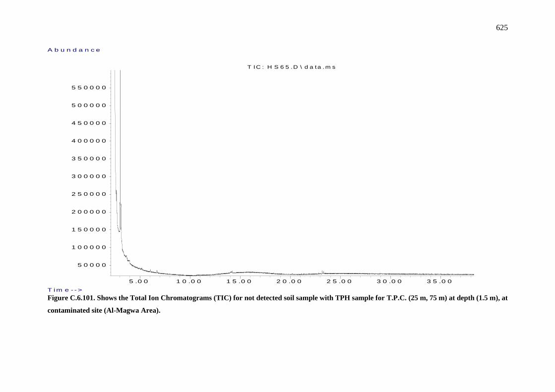
625
Figure C.6.101. Shows the Total Ion Chromatograms (TIC) for not detected soil sample with TPH sample for T.P.C. (25 m, 75 m) at depth (1.5 m), at
contaminated site (Al-Magwa Area).
5 .0 0 1 0 .0 0 1 5 .0 0 2 0 .0 0 2 5 .0 0 3 0 .0 0 3 5 .0 0
5 0 0 0 0
1 0 0 0 0 0
1 5 0 0 0 0
2 0 0 0 0 0
2 5 0 0 0 0
3 0 0 0 0 0
3 5 0 0 0 0
4 0 0 0 0 0
4 5 0 0 0 0
5 0 0 0 0 0
5 5 0 0 0 0
T im e - ->
A b u n d a n c e
T IC : H S 6 5 .D \ d a ta .m s

626
Figure C.6.102. Shows the Total Ion Chromatograms (TIC) for not detected soil sample with TPH sample for T.P.C. (50 m, 75 m) at depth (1.5 m), at
contaminated site (Al-Magwa Area).
5.00 10.00 15.00 20.00 25.00 30.00
200000
400000
600000
800000
1000000
1200000
1400000
1600000
1800000
2000000
2200000
2400000
2600000
2800000
3000000
3200000
3400000
3600000
T im e-->
Abundance
T IC : H S 2 1 .D \ d a ta .m s

627
Figure C.6.103. Shows the Total Ion Chromatograms (TIC) for not detected soil sample with TPH sample for T.P.C. (75 m, 75 m) at depth (1.5 m), at
contaminated site (Al-Magwa Area).
5 . 0 0 1 0 . 0 0 1 5 . 0 0 2 0 . 0 0 2 5 . 0 0 3 0 . 0 0
2 0 0 0 0 0
4 0 0 0 0 0
6 0 0 0 0 0
8 0 0 0 0 0
1 0 0 0 0 0 0
1 2 0 0 0 0 0
1 4 0 0 0 0 0
1 6 0 0 0 0 0
1 8 0 0 0 0 0
2 0 0 0 0 0 0
2 2 0 0 0 0 0
2 4 0 0 0 0 0
2 6 0 0 0 0 0
2 8 0 0 0 0 0
3 0 0 0 0 0 0
3 2 0 0 0 0 0
3 4 0 0 0 0 0
3 6 0 0 0 0 0
3 8 0 0 0 0 0
4 0 0 0 0 0 0
4 2 0 0 0 0 0
4 4 0 0 0 0 0
T i m e - - >
A b u n d a n c e
T I C : H S 1 7 a . D \ d a t a . m s
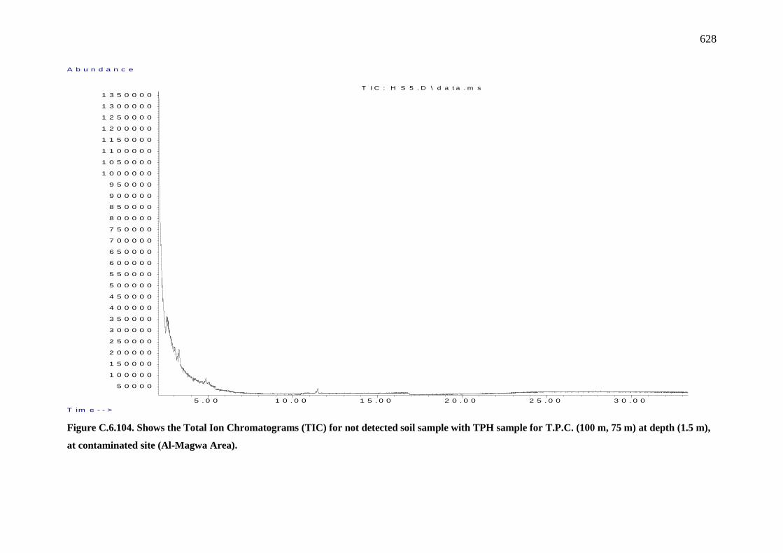
628
Figure C.6.104. Shows the Total Ion Chromatograms (TIC) for not detected soil sample with TPH sample for T.P.C. (100 m, 75 m) at depth (1.5 m),
at contaminated site (Al-Magwa Area).
5 . 0 0 1 0 . 0 0 1 5 . 0 0 2 0 . 0 0 2 5 . 0 0 3 0 . 0 0
5 0 0 0 0
1 0 0 0 0 0
1 5 0 0 0 0
2 0 0 0 0 0
2 5 0 0 0 0
3 0 0 0 0 0
3 5 0 0 0 0
4 0 0 0 0 0
4 5 0 0 0 0
5 0 0 0 0 0
5 5 0 0 0 0
6 0 0 0 0 0
6 5 0 0 0 0
7 0 0 0 0 0
7 5 0 0 0 0
8 0 0 0 0 0
8 5 0 0 0 0
9 0 0 0 0 0
9 5 0 0 0 0
1 0 0 0 0 0 0
1 0 5 0 0 0 0
1 1 0 0 0 0 0
1 1 5 0 0 0 0
1 2 0 0 0 0 0
1 2 5 0 0 0 0
1 3 0 0 0 0 0
1 3 5 0 0 0 0
T im e - - >
A b u n d a n c e
T I C : H S 5 . D \ d a t a . m s

629
Figure C.6.105. Shows the Total Ion Chromatograms (TIC) for not detected soil sample with TPH sample for T.P.C. (0 m, 100 m) at depth (1.5 m), at
contaminated site (Al-Magwa Area).
5 . 0 0 1 0 . 0 0 1 5 . 0 0 2 0 . 0 0 2 5 . 0 0 3 0 . 0 0
5 0 0 0 0 0
1 0 0 0 0 0 0
1 5 0 0 0 0 0
2 0 0 0 0 0 0
2 5 0 0 0 0 0
3 0 0 0 0 0 0
3 5 0 0 0 0 0
4 0 0 0 0 0 0
4 5 0 0 0 0 0
5 0 0 0 0 0 0
5 5 0 0 0 0 0
6 0 0 0 0 0 0
6 5 0 0 0 0 0
T i m e - - >
A b u n d a n c e
T I C : H S 5 3 . D \ d a t a . m s
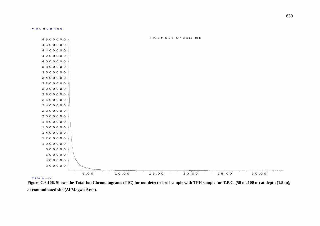
630
Figure C.6.106. Shows the Total Ion Chromatograms (TIC) for not detected soil sample with TPH sample for T.P.C. (50 m, 100 m) at depth (1.5 m),
at contaminated site (Al-Magwa Area).
5 .0 0 1 0 . 0 0 1 5 . 0 0 2 0 . 0 0 2 5 . 0 0 3 0 . 0 0
2 0 0 0 0 0
4 0 0 0 0 0
6 0 0 0 0 0
8 0 0 0 0 0
1 0 0 0 0 0 0
1 2 0 0 0 0 0
1 4 0 0 0 0 0
1 6 0 0 0 0 0
1 8 0 0 0 0 0
2 0 0 0 0 0 0
2 2 0 0 0 0 0
2 4 0 0 0 0 0
2 6 0 0 0 0 0
2 8 0 0 0 0 0
3 0 0 0 0 0 0
3 2 0 0 0 0 0
3 4 0 0 0 0 0
3 6 0 0 0 0 0
3 8 0 0 0 0 0
4 0 0 0 0 0 0
4 2 0 0 0 0 0
4 4 0 0 0 0 0
4 6 0 0 0 0 0
4 8 0 0 0 0 0
T i m e - - >
A b u n d a n c e
T I C : H S 2 7 . D \ d a t a . m s
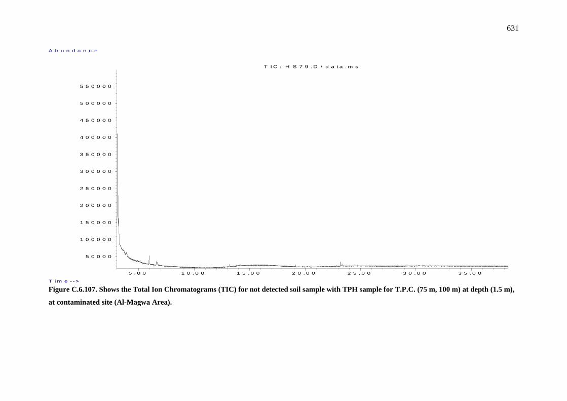
631
Figure C.6.107. Shows the Total Ion Chromatograms (TIC) for not detected soil sample with TPH sample for T.P.C. (75 m, 100 m) at depth (1.5 m),
at contaminated site (Al-Magwa Area).
5 . 0 0 1 0 . 0 0 1 5 . 0 0 2 0 . 0 0 2 5 . 0 0 3 0 . 0 0 3 5 . 0 0
5 0 0 0 0
1 0 0 0 0 0
1 5 0 0 0 0
2 0 0 0 0 0
2 5 0 0 0 0
3 0 0 0 0 0
3 5 0 0 0 0
4 0 0 0 0 0
4 5 0 0 0 0
5 0 0 0 0 0
5 5 0 0 0 0
T im e - - >
A b u n d a n c e
T I C : H S 7 9 . D \ d a t a . m s
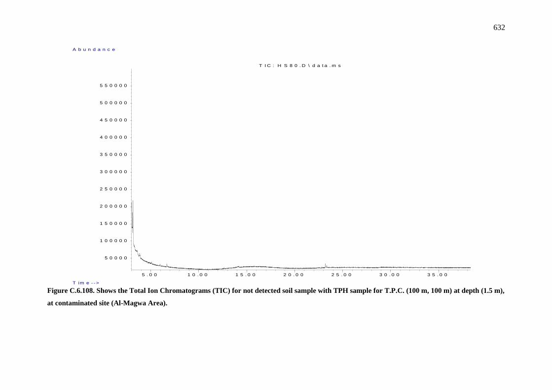
632
Figure C.6.108. Shows the Total Ion Chromatograms (TIC) for not detected soil sample with TPH sample for T.P.C. (100 m, 100 m) at depth (1.5 m),
at contaminated site (Al-Magwa Area).
5 . 0 0 1 0 . 0 0 1 5 . 0 0 2 0 . 0 0 2 5 . 0 0 3 0 . 0 0 3 5 . 0 0
5 0 0 0 0
1 0 0 0 0 0
1 5 0 0 0 0
2 0 0 0 0 0
2 5 0 0 0 0
3 0 0 0 0 0
3 5 0 0 0 0
4 0 0 0 0 0
4 5 0 0 0 0
5 0 0 0 0 0
5 5 0 0 0 0
T im e - - >
A b u n d a n c e
T I C : H S 8 0 . D \ d a t a . m s

633
For Non-Contaminated Samples at depth (0.0 m)

634
Figure C.6.109. Shows the Total Ion Chromatograms (TIC) of non-contaminated soil sample that found to be not detected with TPH for T.P.C. (0 m,
0 m) at depth (0.0 m), at non-contaminated site (Al-Magwa Area).

635
Figure C.6.110. Shows the Total Ion Chromatograms (TIC) of non-contaminated soil sample that found to be not detected with TPH for T.P.C. (100
m, 0 m) at depth (0.0 m), at non-contaminated site (Al-Magwa Area).

636
Figure C.6.111. Shows the Total Ion Chromatograms (TIC) of non-contaminated soil sample that found to be not detected with TPH for T.P.C. (0 m,
100 m) at depth (0.0 m), at non-contaminated site (Al-Magwa Area).

637
Figure C.6.112. Shows the Total Ion Chromatograms (TIC) of non-contaminated soil sample that found to be not detected with TPH for T.P.C. (100
m, 100 m) at depth (0.0 m), at non-contaminated site (Al-Magwa Area).

638
For Non-Contaminated Samples at depth (0.25m)
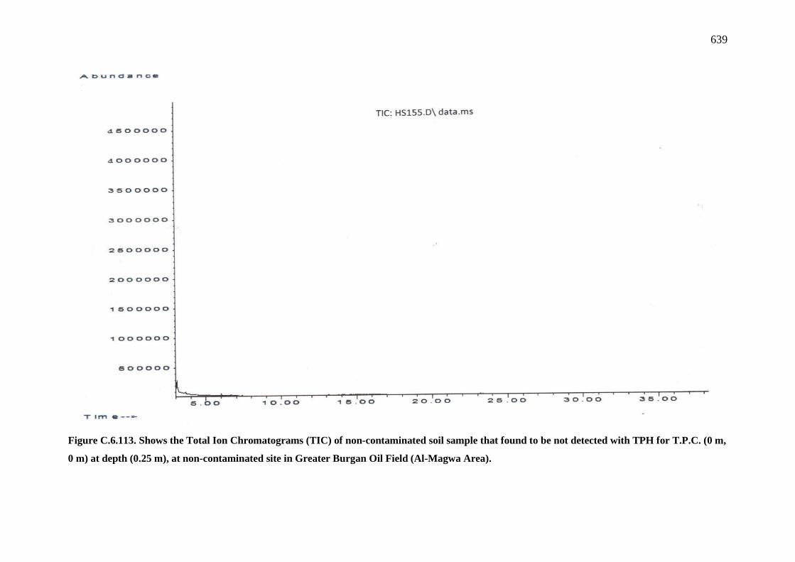
639
Figure C.6.113. Shows the Total Ion Chromatograms (TIC) of non-contaminated soil sample that found to be not detected with TPH for T.P.C. (0 m,
0 m) at depth (0.25 m), at non-contaminated site in Greater Burgan Oil Field (Al-Magwa Area).

640
Figure C.6.114. Shows the Total Ion Chromatograms (TIC) of non-contaminated soil sample that found to be not detected with TPH for coordinate
(100 m, 0 m) at depth (0.25 m), at non-contaminated site (Al-Magwa Area).

641
Figure C.6.115. Shows the Total Ion Chromatograms (TIC) of non-contaminated soil sample that found to be not detected with TPH for T.P.C. (50
m, 50 m) at depth (0.25 m), at non-contaminated site (Al-Magwa Area).
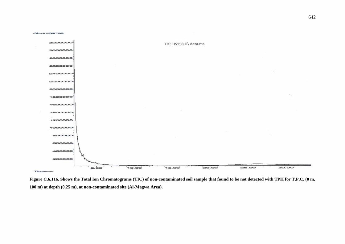
642
Figure C.6.116. Shows the Total Ion Chromatograms (TIC) of non-contaminated soil sample that found to be not detected with TPH for T.P.C. (0 m,
100 m) at depth (0.25 m), at non-contaminated site (Al-Magwa Area).

643
Figure C.6.117. Shows the Total Ion Chromatograms (TIC) of non-contaminated soil sample that found to be not detected with TPH for T.P.C. (100
m, 100 m) at depth (0.25 m), at non-contaminated site (Al-Magwa Area).
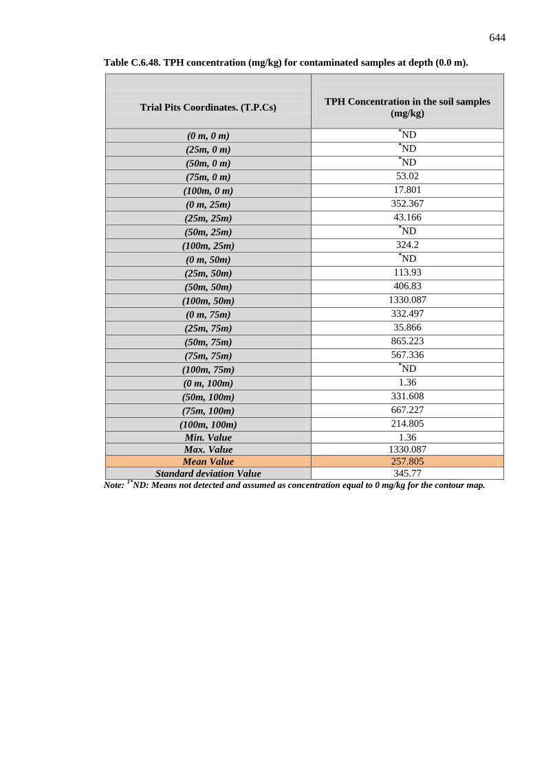
644 Table C.6.48. TPH concentration (mg/kg) for contaminated samples at depth (0.0 m).
Trial Pits Coordinates. (T.P.Cs)
TPH Concentration in the soil samples
(mg/kg)
(0 m, 0 m) *ND
(25m, 0 m) *ND
(50m, 0 m) *ND
(75m, 0 m) 53.02
(100m, 0 m) 17.801
(0 m, 25m) 352.367
(25m, 25m) 43.166
(50m, 25m) *ND
(100m, 25m) 324.2
(0 m, 50m) *ND
(25m, 50m) 113.93
(50m, 50m) 406.83
(100m, 50m) 1330.087
(0 m, 75m) 332.497
(25m, 75m) 35.866
(50m, 75m) 865.223
(75m, 75m) 567.336
(100m, 75m) *ND
(0 m, 100m) 1.36
(50m, 100m) 331.608
(75m, 100m) 667.227
(100m, 100m) 214.805 Min. Value 1.36 Max. Value 1330.087 Mean Value 257.805
Standard deviation Value 345.77 Note: 1*ND: Means not detected and assumed as concentration equal to 0 mg/kg for the contour map.

645
Table C.6.49. TPH concentration (mg/kg) for contaminated samples at depth (0.25m).
Trial Pits Coordinates. (T.P.Cs)
TPH Concentration in the soil samples
(mg/kg)
(0 m, 0 m) *ND (25 m, 0 m) *ND (50 m, 0 m) *ND (75 m, 0 m) *ND (100m, 0 m) 2.532 (0 m, 25 m) 42.3
(25 m, 25 m) *ND (50 m, 25 m) *ND
(100 m, 25 m) *ND (0 m, 50 m) *ND
(25 m, 50 m) 203.486 (50 m, 50 m) 3.506
(100 m, 50 m) *ND (0 m, 75 m) 225.1
(25 m, 75 m) *ND (50 m, 75 m) *ND (75 m, 75 m) *ND
(100 m, 75 m) 1271.038 (0 m, 100 m) *ND
(50 m, 100 m) *ND (75 m, 100 m) 532.378 (100 m, 100 m) *ND
Min. Value 2.532 Max. Value 1271.038 Mean Value 103.651
Standard deviation Value 289.209 Note: *ND: Means not detected and assumed as concentration equal to 0 mg/kg for the contour map.
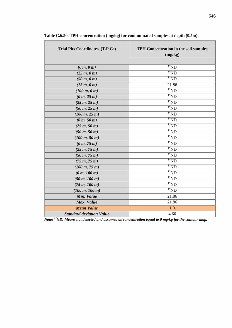
646
Table C.6.50. TPH concentration (mg/kg) for contaminated samples at depth (0.5m).
Trial Pits Coordinates. (T.P.Cs)
TPH Concentration in the soil samples
(mg/kg)
(0 m, 0 m) 1*ND (25 m, 0 m) 1*ND (50 m, 0 m) 1*ND (75 m, 0 m) 21.86 (100 m, 0 m) 1*ND (0 m, 25 m) 1*ND (25 m, 25 m) 1*ND (50 m, 25 m) 1*ND
(100 m, 25 m) 1*ND (0 m, 50 m) 1*ND (25 m, 50 m) 1*ND (50 m, 50 m) 1*ND
(100 m, 50 m) 1*ND (0 m, 75 m) 1*ND (25 m, 75 m) 1*ND (50 m, 75 m) 1*ND (75 m, 75 m) 1*ND
(100 m, 75 m) 1*ND (0 m, 100 m) 1*ND
(50 m, 100 m) 1*ND (75 m, 100 m) 1*ND (100 m, 100 m) 1*ND
Min. Value 21.86 Max. Value 21.86 Mean Value 1.0
Standard deviation Value 4.66 Note: 1*ND: Means not detected and assumed as concentration equal to 0 mg/kg for the contour map.

647
Table C.6.51. The significant p-values via normality Shapiro-Wilk test indicate that the TPH values (mg/kg) of the soil at contaminated site at three different depths (0.0 m, 0.25 m & 0.5 m) follow non-normal distribution.
Table C.6.52. Indicates the significant difference between the TPH variable (mg/kg) in the soil between different depths (0.0 m, 0.25 m & 0.5 m) at contaminated site.

648
APPENDIX D
7. HUMAN HEALTH RISK ASSESSMENT (HHRA) of HYDROCARBON CONTAMINATED SOILS.
Table D.7.1. The summary of Gasoline clean up levels (ppm) (AFCEE, 1996).
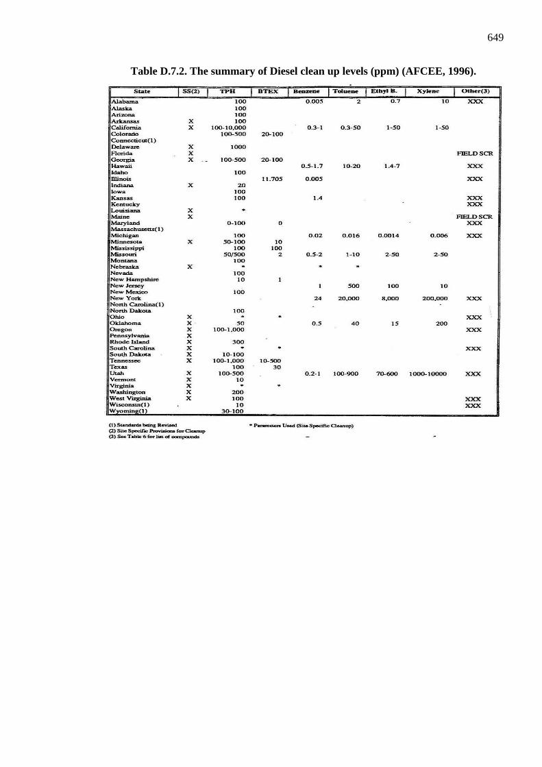
649
Table D.7.2. The summary of Diesel clean up levels (ppm) (AFCEE, 1996).

650
Figure D.7.1. The summary of petroleum product types and TPH and TPH analytical
methods with respect to approximate carbon number and boiling point ranges
(TPHCWG, 1998).
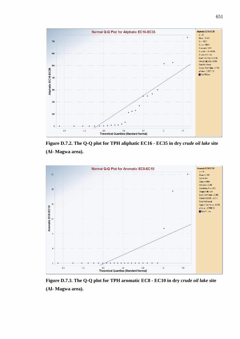
651
Figure D.7.2. The Q-Q plot for TPH aliphatic EC16 - EC35 in dry crude oil lake site
(Al- Magwa area).
Figure D.7.3. The Q-Q plot for TPH aromatic EC8 - EC10 in dry crude oil lake site
(Al- Magwa area).
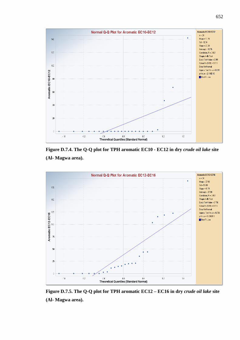
652
Figure D.7.4. The Q-Q plot for TPH aromatic EC10 - EC12 in dry crude oil lake site
(Al- Magwa area).
Figure D.7.5. The Q-Q plot for TPH aromatic EC12 – EC16 in dry crude oil lake site
(Al- Magwa area).

653
Figure D.7.6. The Q-Q plot for TPH aromatic EC16 – EC21 in dry crude oil lake site
(Al- Magwa area).
Figure D.7.7. The Q-Q plot for TPH total fractions in dry crude oil lake site (Al-
Magwa area).

654
Figure D.7.8. The Q-Q plot for Anthracene substance in dry crude oil lake site (Al-
Magwa area).
Figure D.7.9. The Q-Q plot for Phenanthrene substance in dry crude oil lake site (Al-
Magwa area).

655
Figure D.7.10. The 95 % UCLs of the mean concentration (mg/kg) for Aliphatic EC12
- EC16 fraction.
Figure D.7.11. The 95 % UCLs of the mean concentration (mg/kg) for Aliphatic EC16
- EC35 fraction.
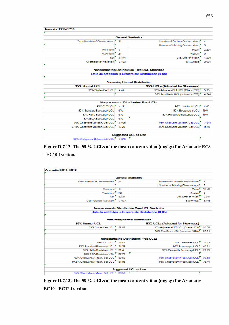
656
Figure D.7.12. The 95 % UCLs of the mean concentration (mg/kg) for Aromatic EC8
- EC10 fraction.
Figure D.7.13. The 95 % UCLs of the mean concentration (mg/kg) for Aromatic
EC10 - EC12 fraction.

657
Figure D.7.14. The 95 % UCLs of the mean concentration (mg/kg) for Aromatic
EC12 - EC16 fraction.
Figure D.7.15. The 95 % UCLs of the mean concentration (mg/kg) for Aromatic
EC16 - EC21 fraction.
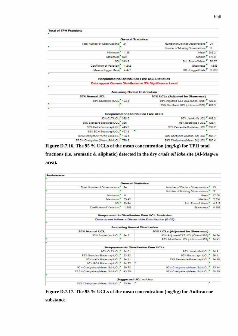
658
Figure D.7.16. The 95 % UCLs of the mean concentration (mg/kg) for TPH total
fractions (i.e. aromatic & aliphatic) detected in the dry crude oil lake site (Al-Magwa
area).
Figure D.7.17. The 95 % UCLs of the mean concentration (mg/kg) for Anthracene
substance.
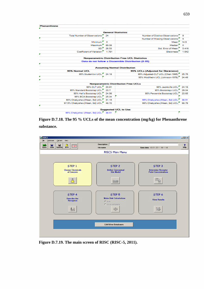
659
Figure D.7.18. The 95 % UCLs of the mean concentration (mg/kg) for Phenanthrene
substance.
Figure D.7.19. The main screen of RISC (RISC-5, 2011).
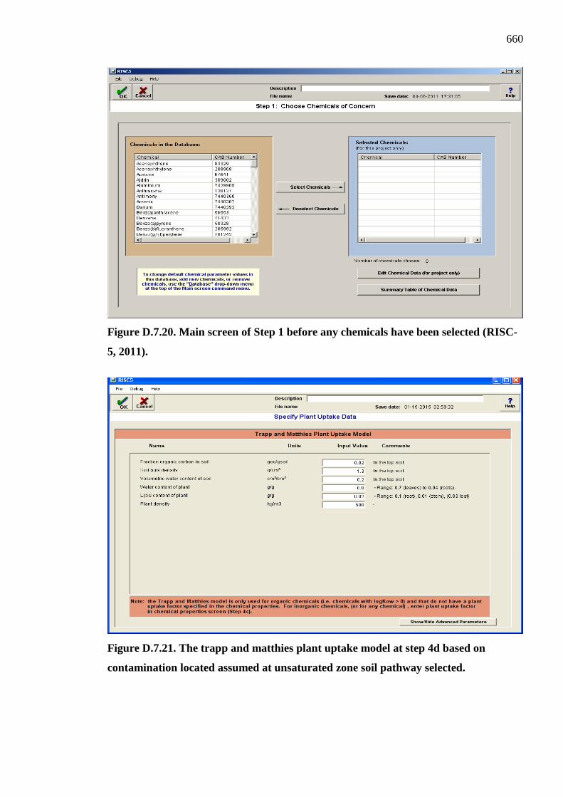
660
Figure D.7.20. Main screen of Step 1 before any chemicals have been selected (RISC-
5, 2011).
Figure D.7.21. The trapp and matthies plant uptake model at step 4d based on
contamination located assumed at unsaturated zone soil pathway selected.

661
Table D.7.3. The equations used to estimate CADD and LADD in accordance with exposure pathways selected.
Exposure
pathways
selected
Exposure pathways
description
Exposure pathways equation
Equation description
References
Ingestion of
Soil or
Sediment.
Adults working
outdoors may ingest soil
through incidental
contact of the mouth
with hands and clothing.
Soil ingestion by
children is often the
primary exposure route
of concern for
contaminated soils
(Paustenbach, 1989a, b).
x 10-6
x 10-6
CADD = chronic average daily dose [mg/kg-day].
LADD = lifetime average daily dose [mg/kg-day].
Cmax = maximum 7-year average concentration of
chemical in soil or sediment [mg/kg].
Cave = time-averaged concentration of chemical in
soil or sediment over the exposure duration [mg/kg].
IR = soil ingestion rate [mg/day].
BIO = bioavailability of chemical in soil [mg/mg].
EF = exposure frequency [events/year].
ED = exposure duration [years].
LT = lifetime = 70 years [by definition].
BW = body weight [kg].
(RISC
-5, 2011)

662
Table D.7.3. Continued.
Exposure
pathways
selected
Exposure pathways
description
Exposure pathways equations
Equation description
References
Dermal Contact
with Soil or Sediment.
Some soil contaminants may
be absorbed across the skin
into the bloodstream.
Absorption will depend upon
the amount of soil in contact
with the skin, the
concentration of chemicals in
soil, the skin surface area
exposed, and the potential for
the chemical to be absorbed
across skin.
x 10-6
x 10-6
Where
Cmax = maximum 7-year average
concentration of chemical in soil or sediment
[mg/kg].
Cave = time-averaged concentration of
chemical in soil or sediment over the exposure
duration [mg/kg].
SA = skin surface area exposed to soil [cm2].
AAF = dermal-soil chemical specific
absorption adjustment factor [mg/mg].
AF = soil-to-skin adherence factor
[mg/cm2/event].
(RISC
-5, 2011)

663
Table D.7.3. Continued.
Exposure
pathways
selected
Exposure pathways
description
Exposure pathways equations
Equation description
References
Inhalation of
Indoor or
Outdoor Air.
In this exposure pathway the
inhalation of chemicals in
breathing space air (either
inside or out) is considered.
Where
Cmax = maximum 7-year concentration of
chemical in outdoor air [mg/m3).
Cave = time-averaged concentration of chemical
in outdoor air over the exposure duration
[mg/m3).
InhR = inhalation rate outdoors [m3/hr].
ET = exposure time outdoors [hr/day].
(RISC
-5, 2011)
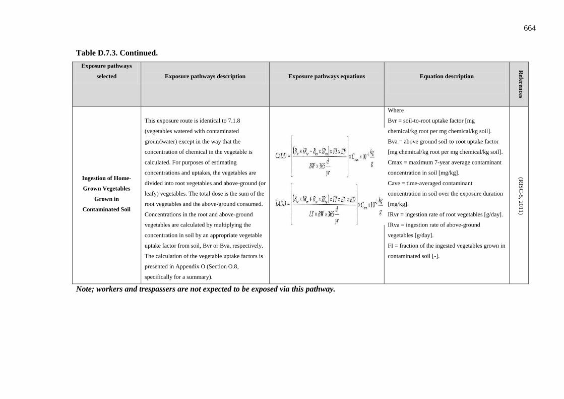
664
Table D.7.3. Continued.
Exposure pathways
selected
Exposure pathways description
Exposure pathways equations
Equation description
References
Ingestion of Home-
Grown Vegetables
Grown in
Contaminated Soil
This exposure route is identical to 7.1.8
(vegetables watered with contaminated
groundwater) except in the way that the
concentration of chemical in the vegetable is
calculated. For purposes of estimating
concentrations and uptakes, the vegetables are
divided into root vegetables and above-ground (or
leafy) vegetables. The total dose is the sum of the
root vegetables and the above-ground consumed.
Concentrations in the root and above-ground
vegetables are calculated by multiplying the
concentration in soil by an appropriate vegetable
uptake factor from soil, Bvr or Bva, respectively.
The calculation of the vegetable uptake factors is
presented in Appendix O (Section O.8,
specifically for a summary).
Where
Bvr = soil-to-root uptake factor [mg
chemical/kg root per mg chemical/kg soil].
Bva = above ground soil-to-root uptake factor
[mg chemical/kg root per mg chemical/kg soil].
Cmax = maximum 7-year average contaminant
concentration in soil [mg/kg].
Cave = time-averaged contaminant
concentration in soil over the exposure duration
[mg/kg].
IRvr = ingestion rate of root vegetables [g/day].
IRva = ingestion rate of above-ground
vegetables [g/day].
FI = fraction of the ingested vegetables grown in
contaminated soil [-].
(RIS
C-5, 2011)
Note; workers and trespassers are not expected to be exposed via this pathway.

665
Table D.7.4. The dialy dose (intake) of risk calculation for Anthracene substance of concern based on
exposure routes assumed in the site.
Exposure pathways Parameters of risk
calculation
Child Resident-
Upper percent
Adult Resident-
Upper percent
Additive Receptor
Case
Ingestion of soil
*CADD (mg/kd-d) 4.5E-04 4.8E-05 -
**LADD (mg/kd-d) 3.8E-05 1.7E-05 5.5E-05
Cancer Risk (-) ***ND ***ND 0.0E+00
Hazard index (-) 1.5E-03 1.6E-04 -
Dermal Contact with Soil
*CADD (mg/kd-d) 1.3E-04 2.3E-05 -
**LADD (mg/kd-d) 1.1E-05 7.9E-06 1.9E-05
Cancer Risk (-) ***ND ***ND 0.0E+00
Hazard index (-) 4.2E-04 7.7E-05 -
Ingestion of Vegetables
*CADD (mg/kd-d) 3.9E-03 1.5E-03
-
**LADD (mg/kd-d) 3.3E-04 5.2E-04 8.5E-04
Cancer Risk (-) ***ND ***ND 0.0E+00
Hazard index (-) 1.3E-02 5.0E-03
-
Inhalation of Outdoor Air
*CADD (mg/kd-d) 1.3E-07 7.6E-09
-
**LADD (mg/kd-d) 1.1E-08 2.6E-09 1.4E-08
Cancer Risk (-) ***ND ***ND 0.0E+00
Hazard index (-) ***ND ***ND -
Inhalation of Particulates
*CADD (mg/kd-d) 2.3E-17 1.4E-18 -
**LADD (mg/kd-d) 2.0E-18 4.7E-19 2.5E-18
Cancer Risk (-) ***ND ***ND 0.0E+00
Hazard index (-) ***ND ***ND -
Note; *CADD: it means chronic average daily dose (RISC-5, 2011). **LADD: it means lifetime average daily dose (RISC-5, 2011). ***ND: it means not detected.

666
Table D.7.5. The daily dose (intake) of risk calculation for Phenanathrene substance of concern based on exposure routes assumed in the site.
Exposure pathways
Parameters of risk calculation
Child Resident-
Upper percent
Adult Resident-
Upper percent
Additive Receptor Case
Ingestion of soil
*CADD (mg/kd-d) 4.7E-04 5.0E-05 -
**LADD (mg/kd-d) 4.0E-05 1.6E-05 5.6E-05
Cancer Risk (-) ***ND ***ND 0.0E+00
Hazard index (-) ***ND ***ND -
Dermal Contact with Soil
*CADD (mg/kd-d) 1.0E-04 1.9E-05 -
**LADD (mg/kd-d) 8.8E-06 5.9E-06 1.5E-05
Cancer Risk (-) ***ND ***ND 0.0E+00
Hazard index (-) ***ND ***ND -
Ingestion of Vegetables
*CADD (mg/kd-d) 4.3E-03 1.7E-03 -
**LADD (mg/kd-d) 3.7E-04 5.3E-04 9.0E-04
Cancer Risk (-) ***ND ***ND 0.0E+00
Hazard index (-) ***ND ***ND -
Inhalation of Outdoor Air
*CADD (mg/kd-d) 2.1E-06 1.3E-07 -
**LADD (mg/kd-d) 1.8E-07 4.0E-08 2.2E-07
Cancer Risk (-) ***ND ***ND 0.0E+00
Hazard index (-) ***ND ***ND -
Inhalation of Particulates
*CADD (mg/kd-d) 2.4E-17 1.4E-18 -
**LADD (mg/kd-d) 2.1E-18 4.6E-19 2.6E-18
Cancer Risk (-) ***ND ***ND 0.0E+00
Hazard index (-) ***ND ***ND -
Note; *CADD: it means chronic average daily dose (RISC-5, 2011). **LADD: it means lifetime average daily dose (RISC-5, 2011). ***ND: it means not detected.

667
Table D.7.6. The daily dose (intake) of risk calculation for TPH aliphatic EC12 - EC16 substance of concern based on exposure routes assumed in the site.
Exposure pathways
Parameters of risk calculation
Child Resident-Upper percent
Adult Resident-Upper percent
Additive Receptor Case
Ingestion of soil
*CADD (mg/kd-d) 2.3E-05 2.1E-06 -
**LADD (mg/kd-d) 2.0E-06 2.1E-07 2.2E-06
Cancer Risk (-) ***ND ***ND 0.0E+00
Hazard index (-) 2.3E-04 2.1E-05 -
Dermal Contact with Soil
*CADD (mg/kd-d) 5.0E-05 7.8E-06 -
**LADD (mg/kd-d) 4.3E-06 7.9E-07 5.1E-06
Cancer Risk (-) ***ND ***ND 0.0E+00
Hazard index (-) 5.0E-04 7.8E-05 -
Ingestion of Vegetables
*CADD (mg/kd-d) 1.8E-04 5.8E-05 -
**LADD (mg/kd-d) 1.5E-05 5.9E-06 2.1E-05
Cancer Risk (-) ***ND ***ND 0.0E+00
Hazard index (-) 1.8E-03 5.8E-04 -
Inhalation of Outdoor Air
*CADD (mg/kd-d) 9.7E-05 5.0E-06 -
**LADD (mg/kd-d) 8.3E-06 5.0E-07 8.8E-06
Cancer Risk (-) ***ND ***ND 0.0E+00
Hazard index (-) 5.1E-05 9.1E-06 -
Inhalation of Particulates
*CADD (mg/kd-d) 1.2E-18 6.1E-20 -
**LADD (mg/kd-d) 1.0E-19 6.1E-21 1.1E-19
Cancer Risk (-) ***ND ***ND 0.0E+00
Hazard index (-) 6.2E-19 1.1E-19 -
Note; *CADD: it means chronic average daily dose (RISC-5, 2011). **LADD: it means lifetime average daily dose (RISC-5, 2011). ***ND: it means not detected.
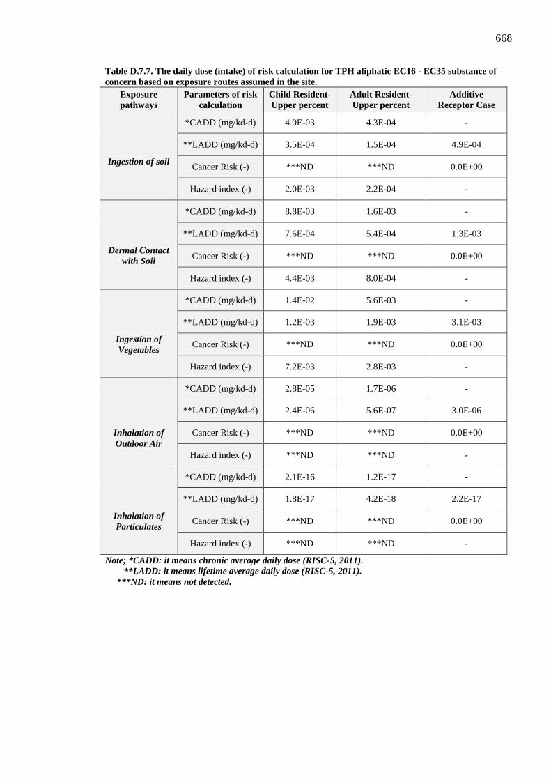
668
Table D.7.7. The daily dose (intake) of risk calculation for TPH aliphatic EC16 - EC35 substance of concern based on exposure routes assumed in the site.
Exposure pathways
Parameters of risk calculation
Child Resident-Upper percent
Adult Resident-Upper percent
Additive Receptor Case
Ingestion of soil
*CADD (mg/kd-d) 4.0E-03 4.3E-04 -
**LADD (mg/kd-d) 3.5E-04 1.5E-04 4.9E-04
Cancer Risk (-) ***ND ***ND 0.0E+00
Hazard index (-) 2.0E-03 2.2E-04 -
Dermal Contact with Soil
*CADD (mg/kd-d) 8.8E-03 1.6E-03 -
**LADD (mg/kd-d) 7.6E-04 5.4E-04 1.3E-03
Cancer Risk (-) ***ND ***ND 0.0E+00
Hazard index (-) 4.4E-03 8.0E-04 -
Ingestion of Vegetables
*CADD (mg/kd-d) 1.4E-02 5.6E-03 -
**LADD (mg/kd-d) 1.2E-03 1.9E-03 3.1E-03
Cancer Risk (-) ***ND ***ND 0.0E+00
Hazard index (-) 7.2E-03 2.8E-03 -
Inhalation of Outdoor Air
*CADD (mg/kd-d) 2.8E-05 1.7E-06 -
**LADD (mg/kd-d) 2.4E-06 5.6E-07 3.0E-06
Cancer Risk (-) ***ND ***ND 0.0E+00
Hazard index (-) ***ND ***ND -
Inhalation of Particulates
*CADD (mg/kd-d) 2.1E-16 1.2E-17 -
**LADD (mg/kd-d) 1.8E-17 4.2E-18 2.2E-17
Cancer Risk (-) ***ND ***ND 0.0E+00
Hazard index (-) ***ND ***ND -
Note; *CADD: it means chronic average daily dose (RISC-5, 2011). **LADD: it means lifetime average daily dose (RISC-5, 2011). ***ND: it means not detected.
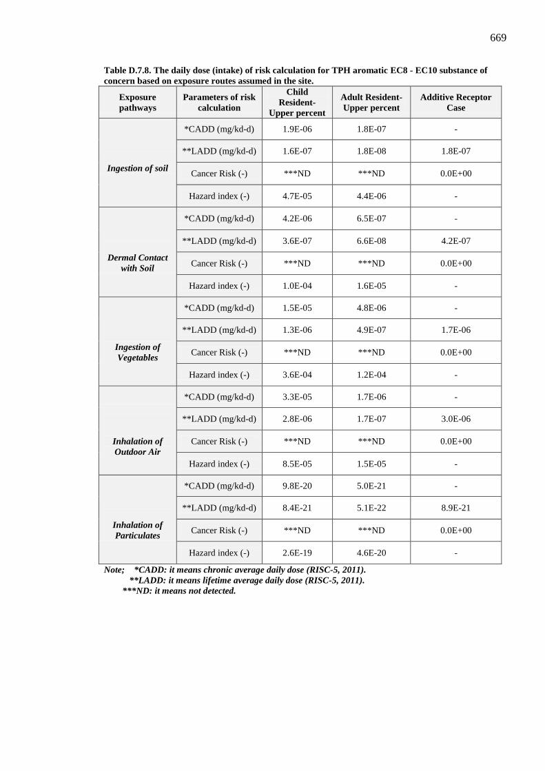
669
Table D.7.8. The daily dose (intake) of risk calculation for TPH aromatic EC8 - EC10 substance of concern based on exposure routes assumed in the site.
Exposure pathways
Parameters of risk calculation
Child Resident-
Upper percent
Adult Resident-Upper percent
Additive Receptor Case
Ingestion of soil
*CADD (mg/kd-d) 1.9E-06 1.8E-07 -
**LADD (mg/kd-d) 1.6E-07 1.8E-08 1.8E-07
Cancer Risk (-) ***ND ***ND 0.0E+00
Hazard index (-) 4.7E-05 4.4E-06 -
Dermal Contact with Soil
*CADD (mg/kd-d) 4.2E-06 6.5E-07 -
**LADD (mg/kd-d) 3.6E-07 6.6E-08 4.2E-07
Cancer Risk (-) ***ND ***ND 0.0E+00
Hazard index (-) 1.0E-04 1.6E-05 -
Ingestion of Vegetables
*CADD (mg/kd-d) 1.5E-05 4.8E-06 -
**LADD (mg/kd-d) 1.3E-06 4.9E-07 1.7E-06
Cancer Risk (-) ***ND ***ND 0.0E+00
Hazard index (-) 3.6E-04 1.2E-04 -
Inhalation of Outdoor Air
*CADD (mg/kd-d) 3.3E-05 1.7E-06 -
**LADD (mg/kd-d) 2.8E-06 1.7E-07 3.0E-06
Cancer Risk (-) ***ND ***ND 0.0E+00
Hazard index (-) 8.5E-05 1.5E-05 -
Inhalation of Particulates
*CADD (mg/kd-d) 9.8E-20 5.0E-21 -
**LADD (mg/kd-d) 8.4E-21 5.1E-22 8.9E-21
Cancer Risk (-) ***ND ***ND 0.0E+00
Hazard index (-) 2.6E-19 4.6E-20 -
Note; *CADD: it means chronic average daily dose (RISC-5, 2011). **LADD: it means lifetime average daily dose (RISC-5, 2011). ***ND: it means not detected.

670
Table D.7.9. The daily dose (intake) of risk calculation for TPH aromatic EC10 - EC12 substance of
concern based on exposure routes assumed in the site.
Exposure pathways
Parameters of risk calculation
Child Resident-Upper percent
Adult Resident-Upper percent
Additive Receptor Case
Ingestion of soil
*CADD (mg/kd-d) 2.6E-05 2.4E-06
-
**LADD (mg/kd-d) 2.3E-06 2.5E-07 2.5E-06
Cancer Risk (-) ***ND ***ND 0.0E+00
Hazard index (-) 6.6E-04 1.7E-04
-
Dermal Contact
with Soil
*CADD (mg/kd-d) 5.8E-05 9.0E-06
-
**LADD (mg/kd-d) 5.0E-06 9.1E-07 5.9E-06
Cancer Risk (-) ***ND ***ND 0.0E+00
Hazard index (-) 1.4E-03 2.3E-04
-
Ingestion of
Vegetables
*CADD (mg/kd-d) 2.5E-04 8.2E-05
-
**LADD (mg/kd-d) 2.1E-05 8.3E-06 2.9E-05
Cancer Risk (-) ***ND ***ND 0.0E+00
Hazard index (-) 6.2E-03 2.1E-03
-
Inhalation of Outdoor Air
*CADD (mg/kd-d) 1.6E-04 8.3E-06 -
**LADD (mg/kd-d) 1.4E-05 8.4E-07 1.5E-05
Cancer Risk (-) ***ND ***ND 0.0E+00
Hazard index (-) 4.2E-04 7.6E-05
-
Inhalation of
Particulates
*CADD (mg/kd-d) 1.4E-18 7.0E-20
-
**LADD (mg/kd-d) 1.2E-19 7.1E-21 1.2E-19
Cancer Risk (-) ***ND ***ND 0.0E+00
Hazard index (-) 3.6E-18 6.4E-19
-
Note; *CADD: it means chronic average daily dose (RISC-5, 2011). **LADD: it means lifetime average daily dose (RISC-5, 2011). ***ND: it means not detected.

671
Table D.7.10. The daily dose (intake) of risk calculation for TPH aromatic EC12 - EC16 substance of concern based on exposure routes assumed in the site.
Exposure pathways
Parameters of risk calculation
Child Resident-Upper percent
Adult Resident-Upper percent
Additive Receptor Case
Ingestion of soil
*CADD (mg/kd-d) 3.3E-04 3.1E-05 -
**LADD (mg/kd-d) 2.8E-05 3.2E-06 3.1E-05
Cancer Risk (-) ***ND ***ND 0.0E+00
Hazard index (-) 8.2E-03 7.7E-04 -
Dermal Contact with Soil
*CADD (mg/kd-d) 7.2E-04 1.1E-04 -
**LADD (mg/kd-d) 6.2E-05 1.2E-05 7.3E-05
Cancer Risk (-) ***ND ***ND 0.0E+00
Hazard index (-) 1.8E-02 2.9E-03 -
Ingestion of Vegetables
*CADD (mg/kd-d) 4.3E-03 1.5E-03 -
**LADD (mg/kd-d) 3.7E-04 1.5E-04 5.2E-04
Cancer Risk (-) ***ND ***ND 0.0E+00
Hazard index (-) 1.1E-01 3.6E-02 -
Inhalation of Outdoor Air
*CADD (mg/kd-d) 3.2E-04 1.7E-05 -
**LADD (mg/kd-d) 2.8E-05 1.7E-06 2.9E-05
Cancer Risk (-) ***ND ***ND 0.0E+00
Hazard index (-) 8.4E-04 1.5E-04 -
Inhalation of Particulates
*CADD (mg/kd-d) 1.7E-17 8.8E-19 -
**LADD (mg/kd-d) 1.5E-18 9.2E-20 1.6E-18
Cancer Risk (-) ***ND ***ND 0.0E+00
Hazard index (-) 4.4E-17 8.1E-18 -
Note; * CADD: it means chronic average daily dose (RISC-5, 2011). **LADD: it means lifetime average daily dose (RISC-5, 2011). ***ND: it means not detected.
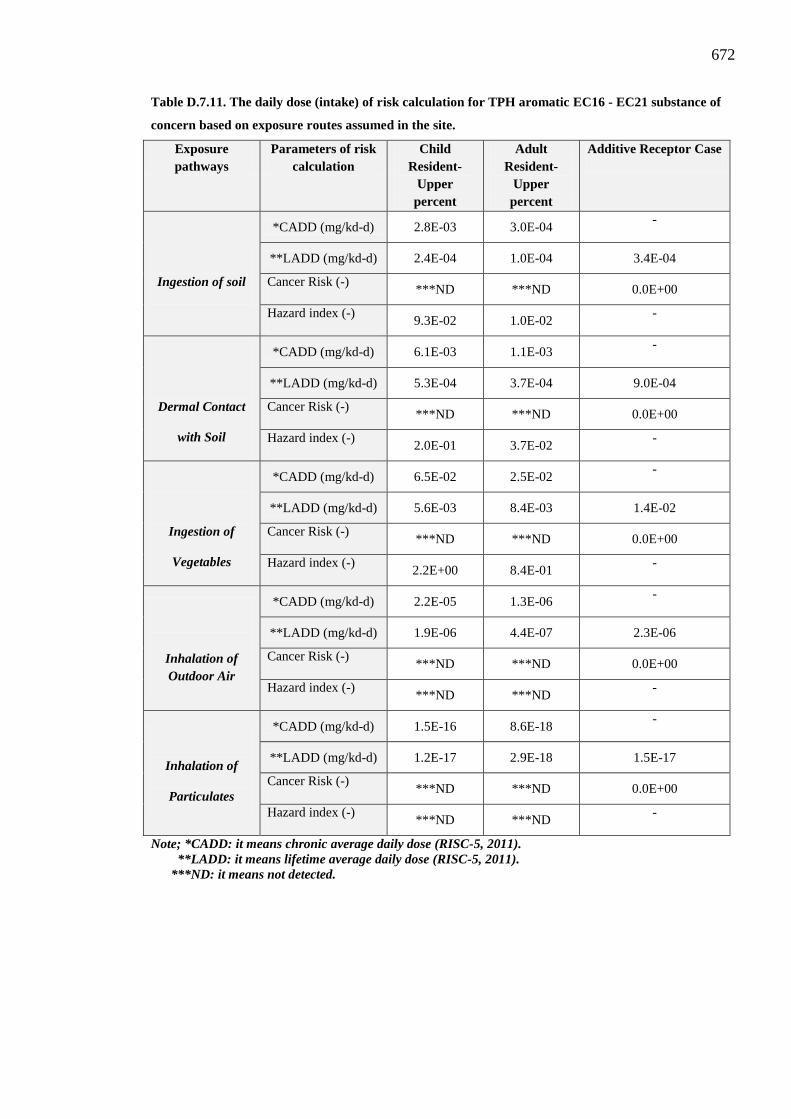
672
Table D.7.11. The daily dose (intake) of risk calculation for TPH aromatic EC16 - EC21 substance of
concern based on exposure routes assumed in the site.
Exposure pathways
Parameters of risk calculation
Child Resident-
Upper percent
Adult Resident-
Upper percent
Additive Receptor Case
Ingestion of soil
*CADD (mg/kd-d) 2.8E-03 3.0E-04 -
**LADD (mg/kd-d) 2.4E-04 1.0E-04 3.4E-04
Cancer Risk (-) ***ND ***ND 0.0E+00
Hazard index (-) 9.3E-02 1.0E-02
-
Dermal Contact
with Soil
*CADD (mg/kd-d) 6.1E-03 1.1E-03 -
**LADD (mg/kd-d) 5.3E-04 3.7E-04 9.0E-04
Cancer Risk (-) ***ND ***ND 0.0E+00
Hazard index (-) 2.0E-01 3.7E-02
-
Ingestion of
Vegetables
*CADD (mg/kd-d) 6.5E-02 2.5E-02 -
**LADD (mg/kd-d) 5.6E-03 8.4E-03 1.4E-02
Cancer Risk (-) ***ND ***ND 0.0E+00
Hazard index (-) 2.2E+00 8.4E-01
-
Inhalation of Outdoor Air
*CADD (mg/kd-d) 2.2E-05 1.3E-06 -
**LADD (mg/kd-d) 1.9E-06 4.4E-07 2.3E-06
Cancer Risk (-) ***ND ***ND 0.0E+00
Hazard index (-) ***ND ***ND -
Inhalation of
Particulates
*CADD (mg/kd-d) 1.5E-16 8.6E-18 -
**LADD (mg/kd-d) 1.2E-17 2.9E-18 1.5E-17
Cancer Risk (-) ***ND ***ND 0.0E+00
Hazard index (-) ***ND ***ND -
Note; *CADD: it means chronic average daily dose (RISC-5, 2011). **LADD: it means lifetime average daily dose (RISC-5, 2011). ***ND: it means not detected.

673
Figure D.7.22. The selected chemical of concern (TPH fraction) for Step (1) of the
RISC-5 software which is used for risk assessment at dry crude oil lake site.
Figure D.7.23. The chosen risk assessment type and the exposure media of
contamination located assumed at unsaturated zone soil pathway in step-2 of the
modelling (RISC-5).

674
Figure D.7.24. The estimating exposure point concentrations of dry crude oil lake site
at step 3 for unsaturated zone soil pathway in RISC-5 modelling.
Figure D.7.25. The enter site data at step 3a in accordance with contamination located
assumed at unsaturated zone soil pathway.
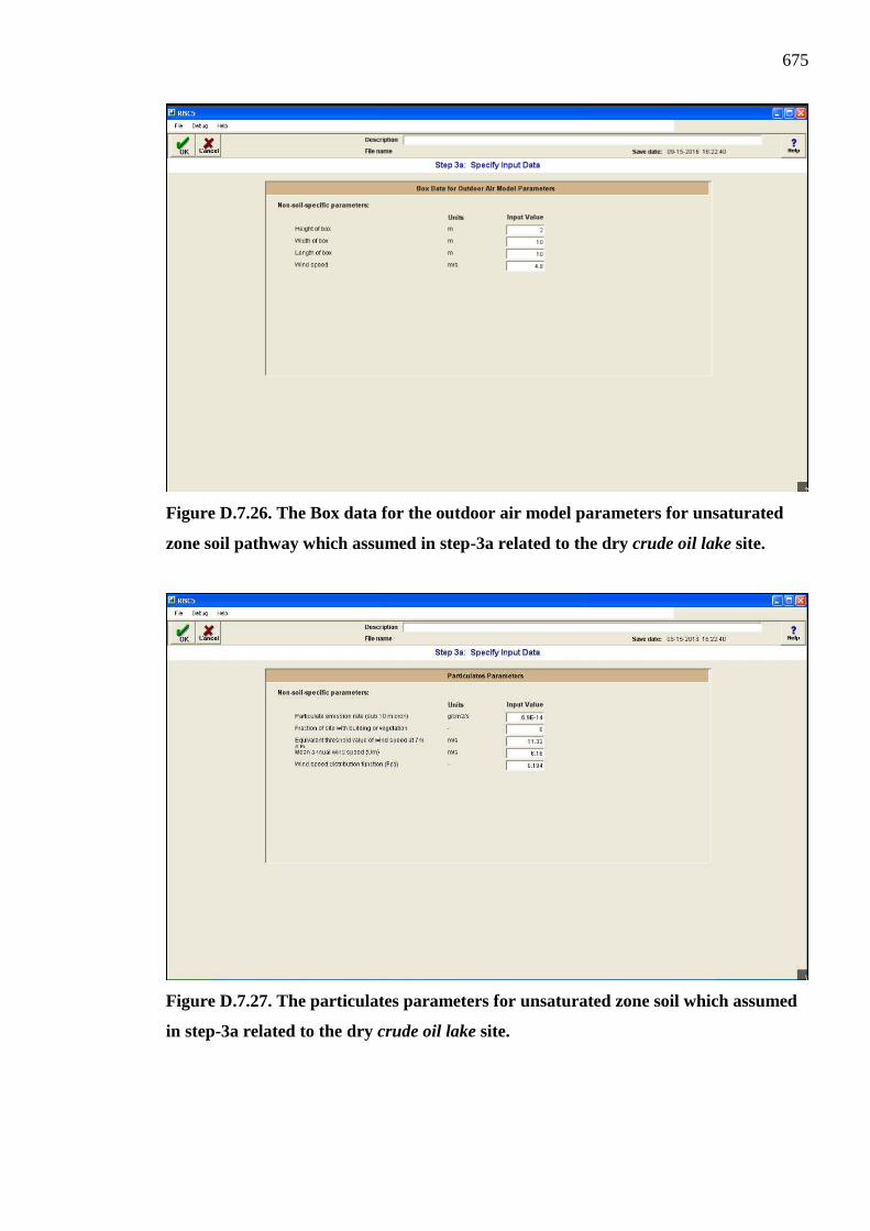
675
Figure D.7.26. The Box data for the outdoor air model parameters for unsaturated
zone soil pathway which assumed in step-3a related to the dry crude oil lake site.
Figure D.7.27. The particulates parameters for unsaturated zone soil which assumed
in step-3a related to the dry crude oil lake site.
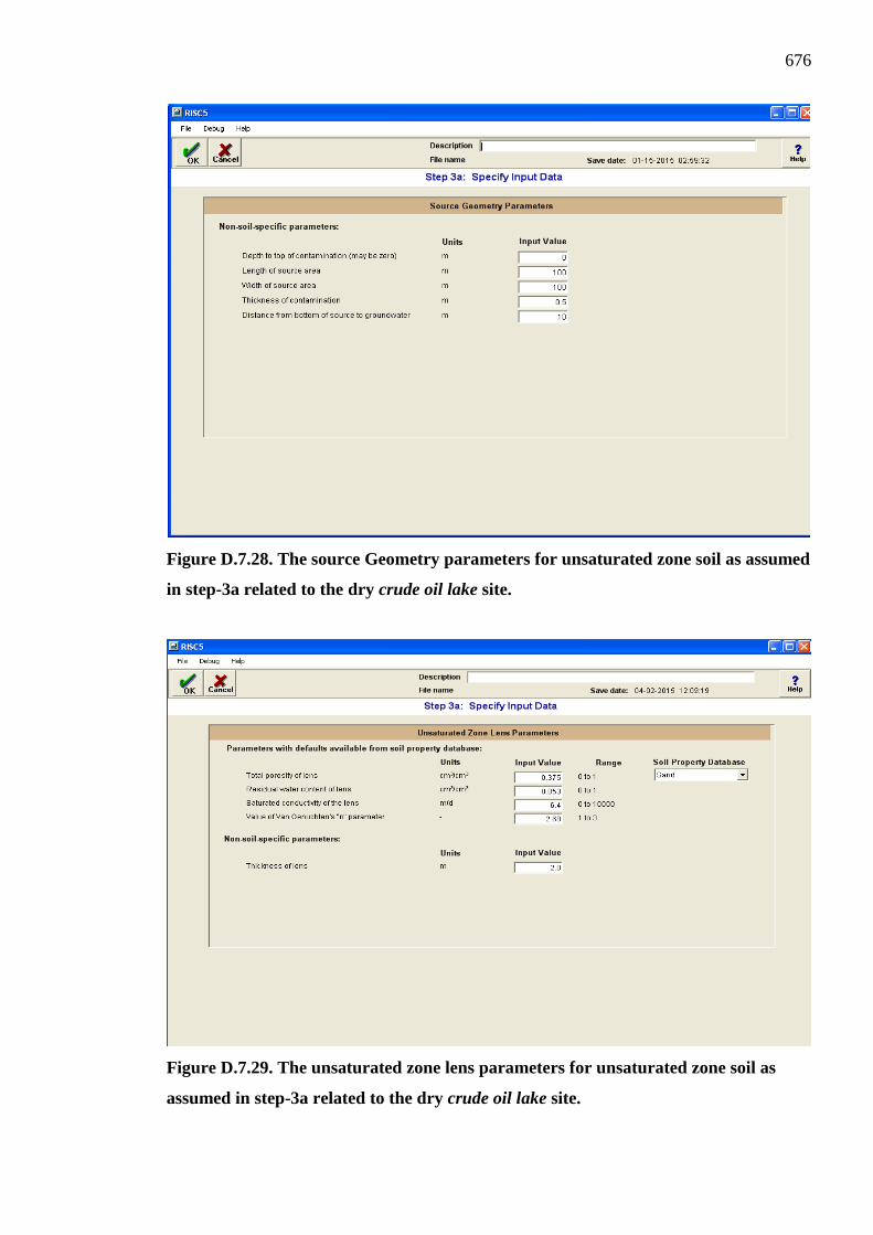
676
Figure D.7.28. The source Geometry parameters for unsaturated zone soil as assumed
in step-3a related to the dry crude oil lake site.
Figure D.7.29. The unsaturated zone lens parameters for unsaturated zone soil as
assumed in step-3a related to the dry crude oil lake site.
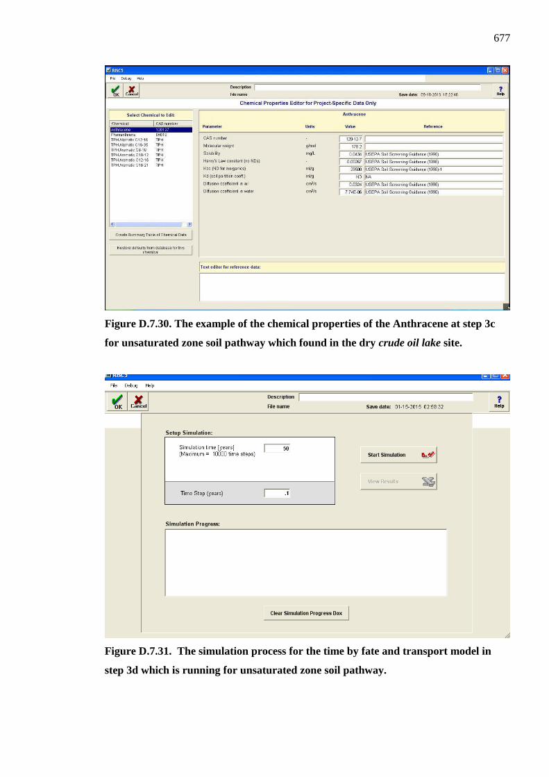
677
Figure D.7.30. The example of the chemical properties of the Anthracene at step 3c
for unsaturated zone soil pathway which found in the dry crude oil lake site.
Figure D.7.31. The simulation process for the time by fate and transport model in
step 3d which is running for unsaturated zone soil pathway.
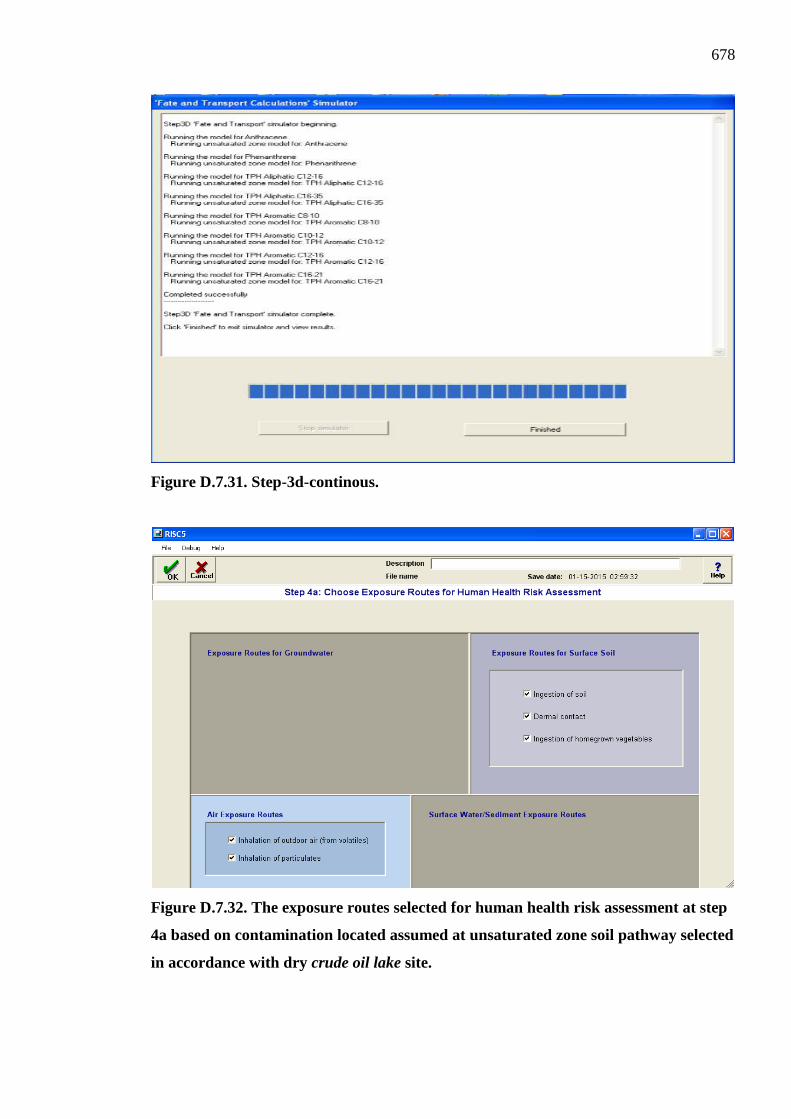
678
Figure D.7.31. Step-3d-continous.
Figure D.7.32. The exposure routes selected for human health risk assessment at step
4a based on contamination located assumed at unsaturated zone soil pathway selected
in accordance with dry crude oil lake site.

679
Figure D.7.33. The types of the receptors to be considered in risk assessment in step
4b as assumed based on contamination located assumed at unsaturated zone soil
pathway selected for dry crude oil lake site.
Figure D.7.34. Review of the chemical properties as example for the specific
anthracene substance concern chosen for risk assessment at step 4c basen on
contamination located assumed at unsaturated zone soil pathway selected.
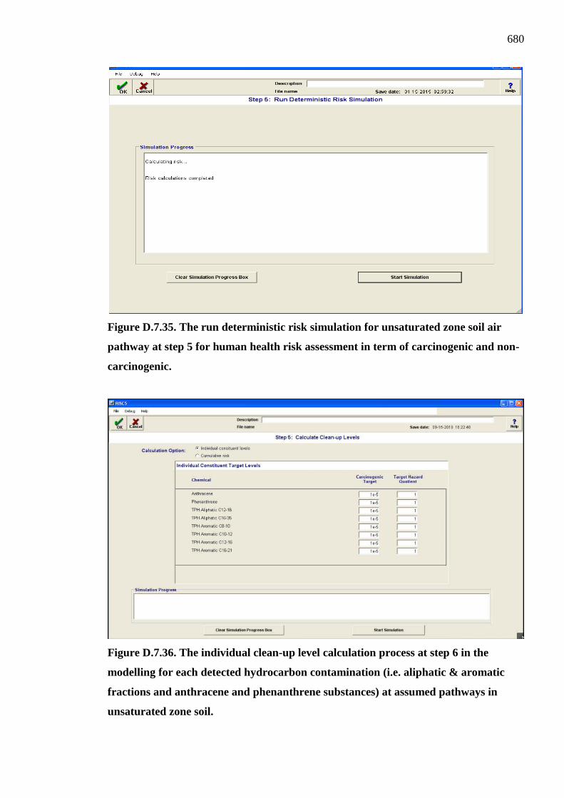
680
Figure D.7.35. The run deterministic risk simulation for unsaturated zone soil air
pathway at step 5 for human health risk assessment in term of carcinogenic and non-
carcinogenic.
Figure D.7.36. The individual clean-up level calculation process at step 6 in the
modelling for each detected hydrocarbon contamination (i.e. aliphatic & aromatic
fractions and anthracene and phenanthrene substances) at assumed pathways in
unsaturated zone soil.
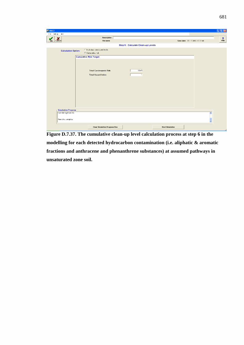
681
Figure D.7.37. The cumulative clean-up level calculation process at step 6 in the
modelling for each detected hydrocarbon contamination (i.e. aliphatic & aromatic
fractions and anthracene and phenanthrene substances) at assumed pathways in
unsaturated zone soil.

682
Table D.7.12. The summary of input Data for Risk Calculation at step 6 (view results) in the
modelling based on the contamination located assumed at unsaturated zone soil pathway.

683
Table D.7.12. Continous.
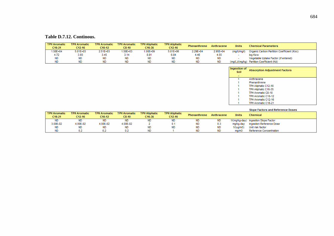
684
Table D.7.12. Continous.
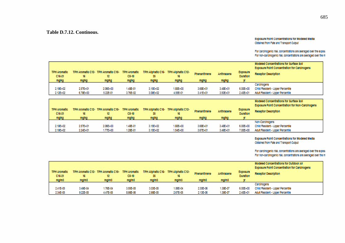
685
Table D.7.12. Continous.
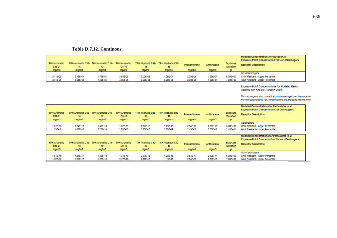
686
Table D.7.12. Continous.
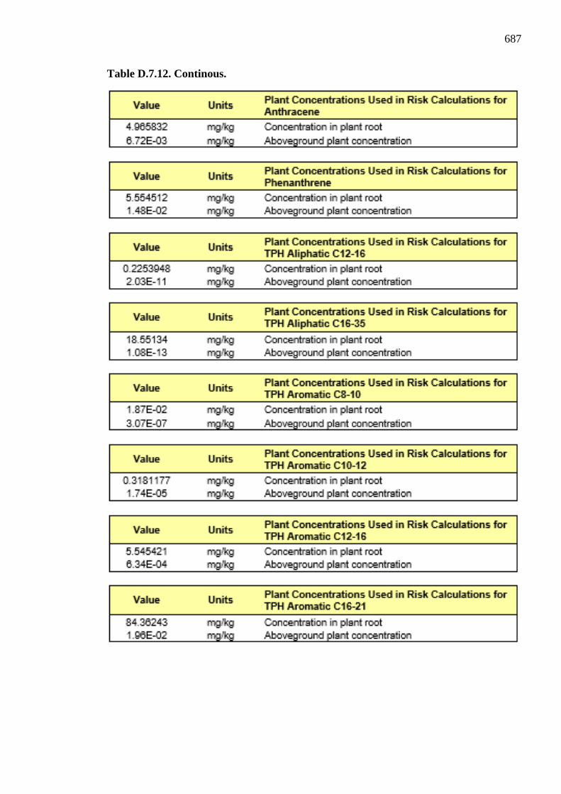
687
Table D.7.12. Continous.

688
Table D.7.12. Continous.

689
Table D.7.12. Continous.
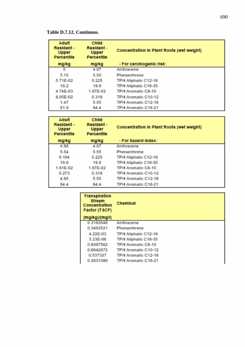
690
Table D.7.12. Continous.

691
Table D.7.12. Continous.
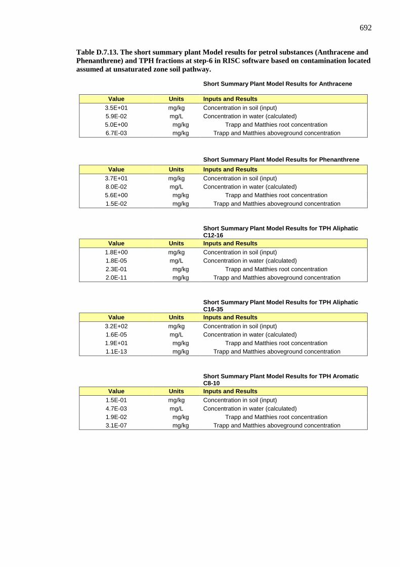
692
Table D.7.13. The short summary plant Model results for petrol substances (Anthracene and Phenanthrene) and TPH fractions at step-6 in RISC software based on contamination located assumed at unsaturated zone soil pathway.
Short Summary Plant Model Results for Anthracene
Inputs and Results Units Value
Concentration in soil (input) mg/kg 3.5E+01 Concentration in water (calculated) mg/L 5.9E-02 Trapp and Matthies root concentration mg/kg 5.0E+00
Trapp and Matthies aboveground concentration mg/kg 6.7E-03
Short Summary Plant Model Results for Phenanthrene
Inputs and Results Units Value
Concentration in soil (input) mg/kg 3.7E+01 Concentration in water (calculated) mg/L 8.0E-02 Trapp and Matthies root concentration mg/kg 5.6E+00 Trapp and Matthies aboveground concentration mg/kg 1.5E-02
Short Summary Plant Model Results for TPH Aliphatic C12-16
Inputs and Results Units Value
Concentration in soil (input) mg/kg 1.8E+00 Concentration in water (calculated) mg/L 1.8E-05 Trapp and Matthies root concentration mg/kg 2.3E-01 Trapp and Matthies aboveground concentration mg/kg 2.0E-11
Short Summary Plant Model Results for TPH Aliphatic C16-35
Inputs and Results Units Value
Concentration in soil (input) mg/kg 3.2E+02
Concentration in water (calculated) mg/L 1.6E-05
Trapp and Matthies root concentration mg/kg 1.9E+01 Trapp and Matthies aboveground concentration mg/kg 1.1E-13
Short Summary Plant Model Results for TPH Aromatic C8-10
Inputs and Results Units Value
Concentration in soil (input) mg/kg 1.5E-01
Concentration in water (calculated) mg/L 4.7E-03 Trapp and Matthies root concentration mg/kg 1.9E-02 Trapp and Matthies aboveground concentration mg/kg 3.1E-07

693
Table D.7.13. Continous.
Short Summary Plant Model Results for TPH Aromatic C10-12
Inputs and Results Units Value
Concentration in soil (input) mg/kg 2.1E+00
Concentration in water (calculated) mg/L 4.1E-02
Trapp and Matthies root concentration mg/kg 3.2E-01 Trapp and Matthies aboveground concentration mg/kg 1.7E-05
Short Summary Plant Model Results for TPH Aromatic C12-16
Inputs and Results Units Value
Concentration in soil (input) mg/kg 2.6E+01 Concentration in water (calculated) mg/L 2.6E-01 Trapp and Matthies root concentration mg/kg 5.5E+00 Trapp and Matthies aboveground concentration mg/kg 6.3E-04
Short Summary Plant Model Results for TPH Aromatic C16-21
Inputs and Results Units Value
Concentration in soil (input) mg/kg 2.2E+02 Concentration in water (calculated) mg/L 6.9E-01 Trapp and Matthies root concentration mg/kg 8.4E+01 Trapp and Matthies aboveground concentration mg/kg 2.0E-02
Short Summary Plant Model Results for Anthracene
Inputs and Results Units Value
Concentration in soil (input) mg/kg 3.5E+01 Concentration in water (calculated) mg/L 5.9E-02 Trapp and Matthies root concentration mg/kg 5.0E+00 Trapp and Matthies aboveground concentration mg/kg 6.8E-03
Short Summary Plant Model Results for Phenanthrene
Inputs and Results Units Value
Concentration in soil (input) mg/kg 3.4E+01 Concentration in water (calculated) mg/L 7.4E-02 Trapp and Matthies root concentration mg/kg 5.1E+00 Trapp and Matthies aboveground concentration mg/kg 1.4E-02
Short Summary Plant Model Results for TPH Aliphatic C12-16
Inputs and Results Units Value
Concentration in soil (input) mg/kg 4.5E-01 Concentration in water (calculated) mg/L 4.5E-06
Trapp and Matthies root concentration mg/kg 5.7E-02
Trapp and Matthies aboveground concentration mg/kg 5.1E-12

694
Table D.7.13. Continous.
Short Summary Plant Model Results for TPH Aliphatic C16-35
Inputs and Results Units Value
Concentration in soil (input) mg/kg 3.1E+02 Concentration in water (calculated) mg/L 1.5E-05 Trapp and Matthies root concentration mg/kg 1.8E+01 Trapp and Matthies aboveground concentration mg/kg 1.1E-13
Short Summary Plant Model Results for TPH Aromatic C8-10
Inputs and Results Units Value
Concentration in soil (input) mg/kg 3.8E-02 Concentration in water (calculated) mg/L 1.2E-03 Trapp and Matthies root concentration mg/kg 4.7E-03 Trapp and Matthies aboveground concentration mg/kg 7.8E-08
Short Summary Plant Model Results for TPH Aromatic C10-12
Inputs and Results Units Value
Concentration in soil (input) mg/kg 5.2E-01 Concentration in water (calculated) mg/L 1.0E-02 Trapp and Matthies root concentration mg/kg 8.1E-02 Trapp and Matthies aboveground concentration mg/kg 4.4E-06
Short Summary Plant Model Results for TPH Aromatic C12-16
Inputs and Results Units Value
Concentration in soil (input) mg/kg 6.8E+00 Concentration in water (calculated) mg/L 6.8E-02 Trapp and Matthies root concentration mg/kg 1.5E+00 Trapp and Matthies aboveground concentration mg/kg 1.7E-04
Short Summary Plant Model Results for TPH Aromatic C16-21
Inputs and Results Units Value
Concentration in soil (input) mg/kg 2.1E+02 Concentration in water (calculated) mg/L 6.7E-01 Trapp and Matthies root concentration mg/kg 8.2E+01 Trapp and Matthies aboveground concentration mg/kg 1.9E-02

695
Table D.7.14. The input Data summary plant Model and their results for petrol substances (Anthracene and Phenanthrene) and TPH fractions at step-6 in RISC software based on contamination located assumed at unsaturated zone soil pathway.
Summary of Plant Model Results for Anthracene
Kd for Anthracene
Organic carbon partitioning coefficient [Koc] ml/g 3.0E+04
Fraction organic carbon [Foc] g/g 2.0E-02
Soil/water partitioning coefficient [Kd] ml/g 5.9E+02
Media Concentrations Units Value
Concentration in soil mg/kg 3.5E+01
Concentration in water mg/L 5.9E-02
Trapp and Matthies -- Calculating Concentration in Roots
logKow (octanol partitioning coefficient) - 4.6E+00
Water content of plant [Wp] g/g 8.0E-01
Lipid content of plant [Lp] g/g 2.0E-02
b correction factor between lipids and octanol - 9.5E-01
Density of plant tissue kg/m3 5.0E+02
Density of water kg/m3 1.0E+03
Water content of the soil cm3/cm3 2.0E-01
Soil bulk density g/cm3 1.3E+00
Partitioning coefficient between roots and water g/g 2.1E+02
Concentration in roots (wet weight) mg/kg 5.0E+00
Aboveground Plant Model Results for Anthracene Units Value
Partitioning between contaminants in leaves and water (Klw)
Klw = (Wp+Lp*((10^logKow) ^bCoeff))*rhoP_to_rhoW
Klw [-] 2.1E+02
Partitioning between contaminants in leaves and air (Kla)
Kla = Klw / Henrys
Kla [-] 7.9E+04
TSCF using first method (TSCF1) [-] 3.4E-02
TSCF using second method (TSCF2) [-] 3.2E-01
Overall TSCF [-] 3.2E-01
Overall rate constant (lambdaE)
lambdaE = lambdaP * fracSun + lambdaM + lambdaG
Photodegradation rate constant 1/d 0.0E+00
Fraction of time in sun [-] 3.0E-01
Metabolism rate constant 1/d 0.0E+00
Growth rate constant 1/d 3.5E-02
Overall rate constant (metabolism, photo. and growth) [a2] 1/s 4.1E-07
Volatilization losses through leaves [a1] 1/s 3.2E-05
Total losses through all mechanisms [a] 1/s 3.2E-05
Total sources [b] kg/m3/s 1.1E-04
Concentration in leaves, not adjusted for water content [b/a] kg/m3 3.4E+00
Concentration in water mg/l 5.9E-02
Time to reach steady-state (95%) d 1.1E+00
Concentration in leaves (wet weight) mg/kg 6.7E-03

696
Table D.7.14. Continous.
Summary of Plant Model Results for Phenanthrene
Kd for Phenanthrene
Organic carbon partitioning coefficient [Koc] ml/g 2.3E+04
Fraction organic carbon [Foc] g/g 2.0E-02
Soil/water partitioning coefficient [Kd] ml/g 4.6E+02
Media Concentrations Units Value
Concentration in soil mg/kg 3.7E+01
Concentration in water mg/L 8.0E-02
Trapp and Matthies -- Calculating Concentration in Roots
logKow (octanol partitioning coefficient) - 4.5E+00
Water content of plant [Wp] g/g 8.0E-01
Lipid content of plant [Lp] g/g 2.0E-02
b correction factor between lipids and octanol - 9.5E-01
Density of plant tissue kg/m3 5.0E+02
Density of water kg/m3 1.0E+03
Water content of the soil cm3/cm3 2.0E-01
Soil bulk density g/cm3 1.3E+00
Partitioning coefficient between roots and water g/g 1.7E+02
Concentration in roots (wet weight) mg/kg 5.6E+00
Aboveground Plant Model Results for Phenanthrene Units Value
Partitioning between contaminants in leaves and water (Klw)
Klw = (Wp+Lp*((10^logKow) ^bCoeff))*rhoP_to_rhoW
Klw [-] 1.7E+02
Partitioning between contaminants in leaves and air (Kla)
Kla = Klw / Henrys
Kla [-] 1.2E+05
TSCF using first method (TSCF1) [-] 4.1E-02
TSCF using second method (TSCF2) [-] 3.5E-01
Overall TSCF [-] 3.5E-01
Overall rate constant (lambdaE)
lambdaE = lambdaP * fracSun + lambdaM + lambdaG
Photodegradation rate constant 1/d 0.0E+00
Fraction of time in sun [-] 3.0E-01
Metabolism rate constant 1/d 0.0E+00
Growth rate constant 1/d 3.5E-02
Overall rate constant (metabolism, photo. and growth) [a2] 1/s 4.1E-07
Volatilization losses through leaves [a1] 1/s 2.1E-05
Total losses through all mechanisms [a] 1/s 2.2E-05
Total sources [b] kg/m3/s 1.6E-04
Concentration in leaves, not adjusted for water content [b/a] kg/m3 7.4E+00
Concentration in water mg/l 8.0E-02
Time to reach steady-state (95%) d 1.6E+00
Concentration in leaves (wet weight) mg/kg 1.5E-02

697
Table D.7.14. Continous.
Summary of Plant Model Results for TPH Aliphatic C12-16
Kd for TPH Aliphatic C12-16
Organic carbon partitioning coefficient [Koc] ml/g 5.0E+06
Fraction organic carbon [Foc] g/g 2.0E-02
Soil/water partitioning coefficient [Kd] ml/g 1.0E+05
Media Concentrations Units Value
Concentration in soil mg/kg 1.8E+00
Concentration in water mg/L 1.8E-05
Trapp and Matthies -- Calculating Concentration in Roots
logKow (octanol partitioning coefficient) - 6.8E+00
Water content of plant [Wp] g/g 8.0E-01
Lipid content of plant [Lp] g/g 2.0E-02
b correction factor between lipids and octanol - 9.5E-01
Density of plant tissue kg/m3 5.0E+02
Density of water kg/m3 1.0E+03
Water content of the soil cm3/cm3 2.0E-01
Soil bulk density g/cm3 1.3E+00
Partitioning coefficient between roots and water g/g 3.1E+04
Concentration in roots (wet weight) mg/kg 2.3E-01
Aboveground Plant Model Results for TPH Aliphatic C12-16 Units Value
Partitioning between contaminants in leaves and water (Klw)
Klw = (Wp+Lp*((10^logKow) ^bCoeff))*rhoP_to_rhoW
Klw [-] 3.1E+04
Partitioning between contaminants in leaves and air (Kla)
Kla = Klw / Henrys
Kla [-] 5.8E+01
TSCF using first method (TSCF1) [-] 2.2E-05
TSCF using second method (TSCF2) [-] 4.2E-03
Overall TSCF [-] 4.2E-03
Overall rate constant (lambdaE)
lambdaE = lambdaP * fracSun + lambdaM + lambdaG
Photodegradation rate constant 1/d 0.0E+00
Fraction of time in sun [-] 3.0E-01
Metabolism rate constant 1/d 0.0E+00
Growth rate constant 1/d 3.5E-02
Overall rate constant (metabolism, photo. and growth) [a2] 1/s 4.1E-07
Volatilization losses through leaves [a1] 1/s 4.3E-02
Total losses through all mechanisms [a] 1/s 4.3E-02
Total sources [b] kg/m3/s 4.4E-10
Concentration in leaves, not adjusted for water content [b/a] kg/m3 1.0E-08
Concentration in water mg/l 1.8E-05
Time to reach steady-state (95%) d 8.1E-04
Concentration in leaves (wet weight) mg/kg 2.0E-11

698
Table D.7.14. Continous.
Summary of Plant Model Results for TPH Aliphatic C16-35
Kd for TPH Aliphatic C16-35
Organic carbon partitioning coefficient [Koc] ml/g 1.0E+09
Fraction organic carbon [Foc] g/g 2.0E-02
Soil/water partitioning coefficient [Kd] ml/g 2.0E+07
Media Concentrations Units Value
Concentration in soil mg/kg 3.2E+02
Concentration in water mg/L 1.6E-05
Trapp and Matthies -- Calculating Concentration in Roots
logKow (octanol partitioning coefficient) - 8.9E+00
Water content of plant [Wp] g/g 8.0E-01
Lipid content of plant [Lp] g/g 2.0E-02
b correction factor between lipids and octanol - 9.5E-01
Density of plant tissue kg/m3 5.0E+02
Density of water kg/m3 1.0E+03
Water content of the soil cm3/cm3 2.0E-01
Soil bulk density g/cm3 1.3E+00
Partitioning coefficient between roots and water g/g 2.9E+06
Concentration in roots (wet weight) mg/kg 1.9E+01
Aboveground Plant Model Results for TPH Aliphatic C16-35 Units Value
Partitioning between contaminants in leaves and water (Klw)
Klw = (Wp+Lp*((10^logKow) ^bCoeff))*rhoP_to_rhoW
Klw [-] 2.9E+06
Partitioning between contaminants in leaves and air (Kla)
Kla = Klw / Henrys
Kla [-] 4.6E+02
TSCF using first method (TSCF1) [-] 6.8E-10
TSCF using second method (TSCF2) [-] 3.2E-06
Overall TSCF [-] 3.2E-06
Overall rate constant (lambdaE)
lambdaE = lambdaP * fracSun + lambdaM + lambdaG
Photodegradation rate constant 1/d 0.0E+00
Fraction of time in sun [-] 3.0E-01
Metabolism rate constant 1/d 0.0E+00
Growth rate constant 1/d 3.5E-02
Overall rate constant (metabolism, photo. and growth) [a2] 1/s 4.1E-07
Volatilization losses through leaves [a1] 1/s 5.4E-03
Total losses through all mechanisms [a] 1/s 5.4E-03
Total sources [b] kg/m3/s 2.9E-13
Concentration in leaves, not adjusted for water content [b/a] kg/m3 5.4E-11
Concentration in water mg/l 1.6E-05
Time to reach steady-state (95%) d 6.4E-03
Concentration in leaves (wet weight) mg/kg 1.1E-13

699
Table D.7.14. Continous.
Summary of Plant Model Results for TPH Aromatic C8-10
Kd for TPH Aromatic C8-10
Organic carbon partitioning coefficient [Koc] ml/g 1.6E+03
Fraction organic carbon [Foc] g/g 2.0E-02
Soil/water partitioning coefficient [Kd] ml/g 3.2E+01
Media Concentrations Units Value
Concentration in soil mg/kg 1.5E-01
Concentration in water mg/L 4.7E-03
Trapp and Matthies -- Calculating Concentration in Roots
logKow (octanol partitioning coefficient) - 3.1E+00
Water content of plant [Wp] g/g 8.0E-01
Lipid content of plant [Lp] g/g 2.0E-02
b correction factor between lipids and octanol - 9.5E-01
Density of plant tissue kg/m3 5.0E+02
Density of water kg/m3 1.0E+03
Water content of the soil cm3/cm3 2.0E-01
Soil bulk density g/cm3 1.3E+00
Partitioning coefficient between roots and water g/g 1.0E+01
Concentration in roots (wet weight) mg/kg 1.9E-02
Aboveground Plant Model Results for TPH Aromatic C8-10 Units Value
Partitioning between contaminants in leaves and water (Klw)
Klw = (Wp+Lp*((10^logKow) ^bCoeff))*rhoP_to_rhoW
Klw [-] 1.0E+01
Partitioning between contaminants in leaves and air (Kla)
Kla = Klw / Henrys
Kla [-] 2.0E+01
TSCF using first method (TSCF1) [-] 3.7E-01
TSCF using second method (TSCF2) [-] 7.0E-01
Overall TSCF [-] 7.0E-01
Overall rate constant (lambdaE)
lambdaE = lambdaP * fracSun + lambdaM + lambdaG
Photodegradation rate constant 1/d 0.0E+00
Fraction of time in sun [-] 3.0E-01
Metabolism rate constant 1/d 0.0E+00
Growth rate constant 1/d 3.5E-02
Overall rate constant (metabolism, photo. and growth) [a2] 1/s 4.1E-07
Volatilization losses through leaves [a1] 1/s 1.2E-01
Total losses through all mechanisms [a] 1/s 1.2E-01
Total sources [b] kg/m3/s 1.9E-05
Concentration in leaves, not adjusted for water content [b/a] kg/m3 1.5E-04
Concentration in water mg/l 4.7E-03
Time to reach steady-state (95%) d 2.8E-04
Concentration in leaves (wet weight) mg/kg 3.1E-07

700
Table D.7.14. Continous.
Summary of Plant Model Results for TPH Aromatic C10-12
Kd for TPH Aromatic C10-12
Organic carbon partitioning coefficient [Koc] ml/g 2.5E+03
Fraction organic carbon [Foc] g/g 2.0E-02
Soil/water partitioning coefficient [Kd] ml/g 5.0E+01
Media Concentrations Units Value
Concentration in soil mg/kg 2.1E+00
Concentration in water mg/L 4.1E-02
Trapp and Matthies -- Calculating Concentration in Roots
logKow (octanol partitioning coefficient) - 3.5E+00
Water content of plant [Wp] g/g 8.0E-01
Lipid content of plant [Lp] g/g 2.0E-02
b correction factor between lipids and octanol - 9.5E-01
Density of plant tissue kg/m3 5.0E+02
Density of water kg/m3 1.0E+03
Water content of the soil cm3/cm3 2.0E-01
Soil bulk density g/cm3 1.3E+00
Partitioning coefficient between roots and water g/g 1.9E+01
Concentration in roots (wet weight) mg/kg 3.2E-01
Aboveground Plant Model Results for TPH Aromatic C10-12 Units Value
Partitioning between contaminants in leaves and water (Klw)
Klw = (Wp+Lp*((10^logKow) ^bCoeff))*rhoP_to_rhoW
Klw [-] 1.9E+01
Partitioning between contaminants in leaves and air (Kla)
Kla = Klw / Henrys
Kla [-] 1.4E+02
TSCF using first method (TSCF1) [-] 2.5E-01
TSCF using second method (TSCF2) [-] 6.6E-01
Overall TSCF [-] 6.6E-01
Overall rate constant (lambdaE)
lambdaE = lambdaP * fracSun + lambdaM + lambdaG
Photodegradation rate constant 1/d 0.0E+00
Fraction of time in sun [-] 3.0E-01
Metabolism rate constant 1/d 0.0E+00
Growth rate constant 1/d 3.5E-02
Overall rate constant (metabolism, photo. and growth) [a2] 1/s 4.1E-07
Volatilization losses through leaves [a1] 1/s 1.8E-02
Total losses through all mechanisms [a] 1/s 1.8E-02
Total sources [b] kg/m3/s 1.6E-04
Concentration in leaves, not adjusted for water content [b/a] kg/m3 8.7E-03
Concentration in water mg/l 4.1E-02
Time to reach steady-state (95%) d 1.9E-03
Concentration in leaves (wet weight) mg/kg 1.7E-05
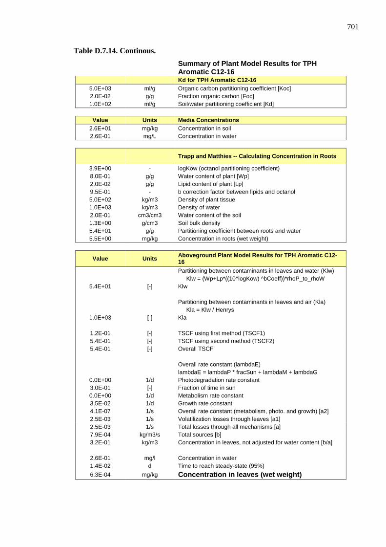
701
Table D.7.14. Continous.
Summary of Plant Model Results for TPH Aromatic C12-16
Kd for TPH Aromatic C12-16
Organic carbon partitioning coefficient [Koc] ml/g 5.0E+03
Fraction organic carbon [Foc] g/g 2.0E-02
Soil/water partitioning coefficient [Kd] ml/g 1.0E+02
Media Concentrations Units Value
Concentration in soil mg/kg 2.6E+01
Concentration in water mg/L 2.6E-01
Trapp and Matthies -- Calculating Concentration in Roots
logKow (octanol partitioning coefficient) - 3.9E+00
Water content of plant [Wp] g/g 8.0E-01
Lipid content of plant [Lp] g/g 2.0E-02
b correction factor between lipids and octanol - 9.5E-01
Density of plant tissue kg/m3 5.0E+02
Density of water kg/m3 1.0E+03
Water content of the soil cm3/cm3 2.0E-01
Soil bulk density g/cm3 1.3E+00
Partitioning coefficient between roots and water g/g 5.4E+01
Concentration in roots (wet weight) mg/kg 5.5E+00
Aboveground Plant Model Results for TPH Aromatic C12-16 Units Value
Partitioning between contaminants in leaves and water (Klw)
Klw = (Wp+Lp*((10^logKow) ^bCoeff))*rhoP_to_rhoW
Klw [-] 5.4E+01
Partitioning between contaminants in leaves and air (Kla)
Kla = Klw / Henrys
Kla [-] 1.0E+03
TSCF using first method (TSCF1) [-] 1.2E-01
TSCF using second method (TSCF2) [-] 5.4E-01
Overall TSCF [-] 5.4E-01
Overall rate constant (lambdaE)
lambdaE = lambdaP * fracSun + lambdaM + lambdaG
Photodegradation rate constant 1/d 0.0E+00
Fraction of time in sun [-] 3.0E-01
Metabolism rate constant 1/d 0.0E+00
Growth rate constant 1/d 3.5E-02
Overall rate constant (metabolism, photo. and growth) [a2] 1/s 4.1E-07
Volatilization losses through leaves [a1] 1/s 2.5E-03
Total losses through all mechanisms [a] 1/s 2.5E-03
Total sources [b] kg/m3/s 7.9E-04
Concentration in leaves, not adjusted for water content [b/a] kg/m3 3.2E-01
Concentration in water mg/l 2.6E-01
Time to reach steady-state (95%) d 1.4E-02
Concentration in leaves (wet weight) mg/kg 6.3E-04

702
Table D.7.14. Continous.
Summary of Plant Model Results for TPH Aromatic C16-21
Kd for TPH Aromatic C16-21
Organic carbon partitioning coefficient [Koc] ml/g 1.6E+04
Fraction organic carbon [Foc] g/g 2.0E-02
Soil/water partitioning coefficient [Kd] ml/g 3.2E+02
Media Concentrations Units Value
Concentration in soil mg/kg 2.2E+02
Concentration in water mg/L 6.9E-01
Trapp and Matthies -- Calculating Concentration in Roots
logKow (octanol partitioning coefficient) - 4.7E+00
Water content of plant [Wp] g/g 8.0E-01
Lipid content of plant [Lp] g/g 2.0E-02
b correction factor between lipids and octanol - 9.5E-01
Density of plant tissue kg/m3 5.0E+02
Density of water kg/m3 1.0E+03
Water content of the soil cm3/cm3 2.0E-01
Soil bulk density g/cm3 1.3E+00
Partitioning coefficient between roots and water g/g 3.0E+02
Concentration in roots (wet weight) mg/kg 8.4E+01
Aboveground Plant Model Results for TPH Aromatic C16-21 Units Value
Partitioning between contaminants in leaves and water (Klw)
Klw = (Wp+Lp*((10^logKow) ^bCoeff))*rhoP_to_rhoW
Klw [-] 3.0E+02
Partitioning between contaminants in leaves and air (Kla)
Kla = Klw / Henrys
Kla [-] 2.3E+04
TSCF using first method (TSCF1) [-] 2.3E-02
TSCF using second method (TSCF2) [-] 2.6E-01
Overall TSCF [-] 2.6E-01
Overall rate constant (lambdaE)
lambdaE = lambdaP * fracSun + lambdaM + lambdaG
Photodegradation rate constant 1/d 0.0E+00
Fraction of time in sun [-] 3.0E-01
Metabolism rate constant 1/d 0.0E+00
Growth rate constant 1/d 3.5E-02
Overall rate constant (metabolism, photo. and growth) [a2] 1/s 4.1E-07
Volatilization losses through leaves [a1] 1/s 1.1E-04
Total losses through all mechanisms [a] 1/s 1.1E-04
Total sources [b] kg/m3/s 1.0E-03
Concentration in leaves, not adjusted for water content [b/a] kg/m3 9.8E+00
Concentration in water mg/l 6.9E-01
Time to reach steady-state (95%) d 3.2E-01
Concentration in leaves (wet weight) mg/kg 2.0E-02
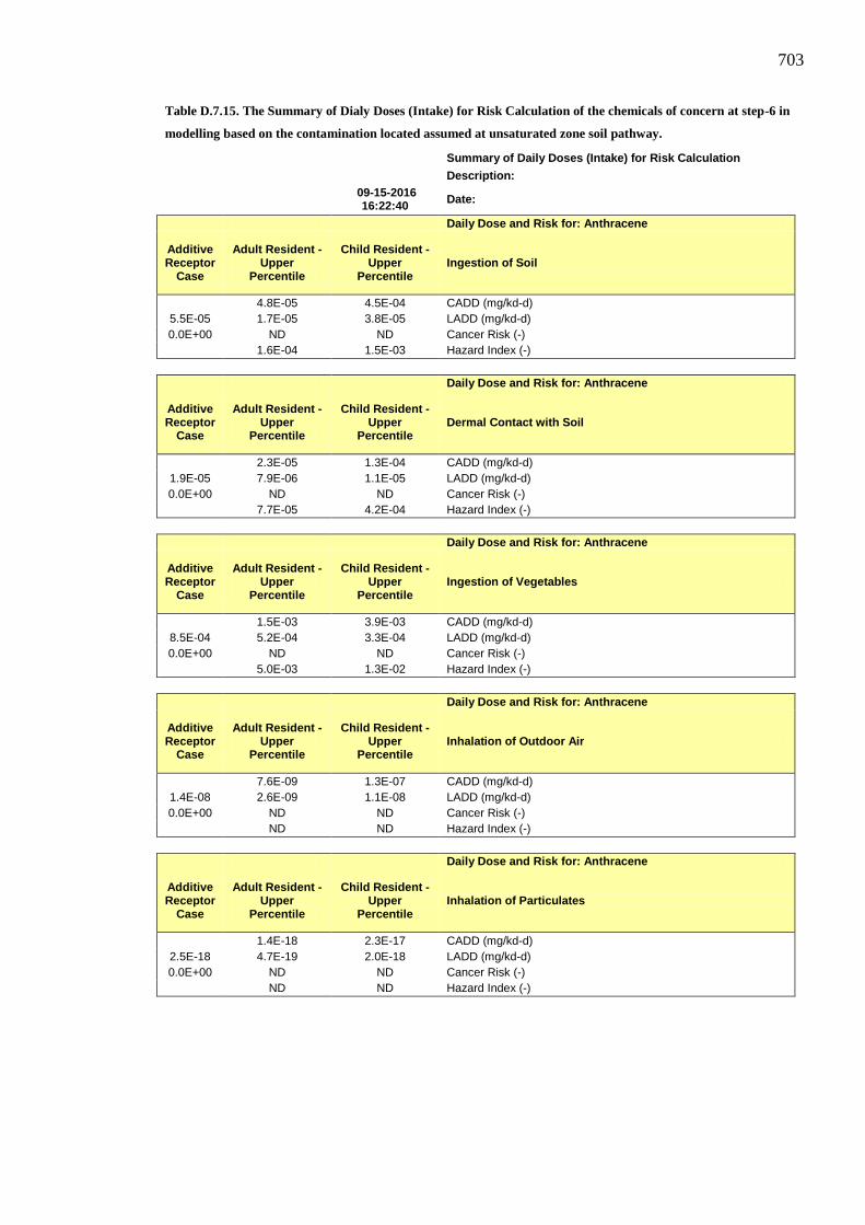
703
Table D.7.15. The Summary of Dialy Doses (Intake) for Risk Calculation of the chemicals of concern at step-6 in
modelling based on the contamination located assumed at unsaturated zone soil pathway.
Summary of Daily Doses (Intake) for Risk Calculation
Description:
Date: 09-15-2016
16:22:40
Daily Dose and Risk for: Anthracene
Ingestion of Soil Child Resident -
Upper Percentile
Adult Resident - Upper
Percentile
Additive Receptor
Case
CADD (mg/kd-d) 4.5E-04 4.8E-05
LADD (mg/kd-d) 3.8E-05 1.7E-05 5.5E-05
Cancer Risk (-) ND ND 0.0E+00
Hazard Index (-) 1.5E-03 1.6E-04
Daily Dose and Risk for: Anthracene
Dermal Contact with Soil Child Resident -
Upper Percentile
Adult Resident - Upper
Percentile
Additive Receptor
Case
CADD (mg/kd-d) 1.3E-04 2.3E-05
LADD (mg/kd-d) 1.1E-05 7.9E-06 1.9E-05
Cancer Risk (-) ND ND 0.0E+00
Hazard Index (-) 4.2E-04 7.7E-05
Daily Dose and Risk for: Anthracene
Ingestion of Vegetables Child Resident -
Upper Percentile
Adult Resident - Upper
Percentile
Additive Receptor
Case
CADD (mg/kd-d) 3.9E-03 1.5E-03
LADD (mg/kd-d) 3.3E-04 5.2E-04 8.5E-04
Cancer Risk (-) ND ND 0.0E+00
Hazard Index (-) 1.3E-02 5.0E-03
Daily Dose and Risk for: Anthracene
Inhalation of Outdoor Air Child Resident -
Upper Percentile
Adult Resident - Upper
Percentile
Additive Receptor
Case
CADD (mg/kd-d) 1.3E-07 7.6E-09
LADD (mg/kd-d) 1.1E-08 2.6E-09 1.4E-08
Cancer Risk (-) ND ND 0.0E+00
Hazard Index (-) ND ND
Daily Dose and Risk for: Anthracene
Inhalation of Particulates Child Resident -
Upper Percentile
Adult Resident - Upper
Percentile
Additive Receptor
Case
CADD (mg/kd-d) 2.3E-17 1.4E-18
LADD (mg/kd-d) 2.0E-18 4.7E-19 2.5E-18
Cancer Risk (-) ND ND 0.0E+00
Hazard Index (-) ND ND

704
Table D.7.15. Continous.
Daily Dose and Risk for: Phenanthrene
Ingestion of Soil Child Resident
- Upper Percentile
Adult Resident -
Upper Percentile
Additive Receptor Case
CADD (mg/kd-d) 4.7E-04 5.0E-05
LADD (mg/kd-d) 4.0E-05 1.6E-05 5.6E-05
Cancer Risk (-) ND ND 0.0E+00
Hazard Index (-) ND ND
Daily Dose and Risk for: Phenanthrene
Dermal Contact with Soil Child Resident
- Upper Percentile
Adult Resident -
Upper Percentile
Additive Receptor Case
CADD (mg/kd-d) 1.0E-04 1.9E-05
LADD (mg/kd-d) 8.8E-06 5.9E-06 1.5E-05
Cancer Risk (-) ND ND 0.0E+00
Hazard Index (-) ND ND
Daily Dose and Risk for: Phenanthrene
Ingestion of Vegetables Child Resident
- Upper Percentile
Adult Resident -
Upper Percentile
Additive Receptor Case
CADD (mg/kd-d) 4.3E-03 1.7E-03
LADD (mg/kd-d) 3.7E-04 5.3E-04 9.0E-04
Cancer Risk (-) ND ND 0.0E+00
Hazard Index (-) ND ND
Daily Dose and Risk for: Phenanthrene
Inhalation of Outdoor Air Child Resident
- Upper Percentile
Adult Resident -
Upper Percentile
Additive Receptor Case
CADD (mg/kd-d) 2.1E-06 1.3E-07
LADD (mg/kd-d) 1.8E-07 4.0E-08 2.2E-07
Cancer Risk (-) ND ND 0.0E+00
Hazard Index (-) ND ND
Daily Dose and Risk for: Phenanthrene
Inhalation of Particulates Child Resident
- Upper Percentile
Adult Resident -
Upper Percentile
Additive Receptor Case
CADD (mg/kd-d) 2.4E-17 1.4E-18
LADD (mg/kd-d) 2.1E-18 4.6E-19 2.6E-18
Cancer Risk (-) ND ND 0.0E+00
Hazard Index (-) ND ND

705
Table D.7.15. Continous.
Daily Dose and Risk for: TPH Aliphatic C12-16
Ingestion of Soil Child Resident - Upper Percentile
Adult Resident - Upper Percentile
Additive Receptor Case
CADD (mg/kd-d) 2.3E-05 2.1E-06
LADD (mg/kd-d) 2.0E-06 2.1E-07 2.2E-06
Cancer Risk (-) ND ND 0.0E+00
Hazard Index (-) 2.3E-04 2.1E-05
Daily Dose and Risk for: TPH Aliphatic C12-16
Dermal Contact with Soil Child Resident - Upper Percentile
Adult Resident - Upper Percentile
Additive Receptor Case
CADD (mg/kd-d) 5.0E-05 7.8E-06
LADD (mg/kd-d) 4.3E-06 7.9E-07 5.1E-06
Cancer Risk (-) ND ND 0.0E+00
Hazard Index (-) 5.0E-04 7.8E-05
Daily Dose and Risk for: TPH Aliphatic C12-16
Ingestion of Vegetables Child Resident - Upper Percentile
Adult Resident - Upper Percentile
Additive Receptor Case
CADD (mg/kd-d) 1.8E-04 5.8E-05
LADD (mg/kd-d) 1.5E-05 5.9E-06 2.1E-05
Cancer Risk (-) ND ND 0.0E+00
Hazard Index (-) 1.8E-03 5.8E-04
Daily Dose and Risk for: TPH Aliphatic C12-16
Inhalation of Outdoor Air Child Resident - Upper Percentile
Adult Resident - Upper Percentile
Additive Receptor Case
CADD (mg/kd-d) 9.7E-05 5.0E-06
LADD (mg/kd-d) 8.3E-06 5.0E-07 8.8E-06
Cancer Risk (-) ND ND 0.0E+00
Hazard Index (-) 5.1E-05 9.1E-06
Daily Dose and Risk for: TPH Aliphatic C12-16
Inhalation of Particulates Child Resident - Upper Percentile
Adult Resident - Upper Percentile
Additive Receptor Case
CADD (mg/kd-d) 1.2E-18 6.1E-20
LADD (mg/kd-d) 1.0E-19 6.1E-21 1.1E-19
Cancer Risk (-) ND ND 0.0E+00
Hazard Index (-) 6.2E-19 1.1E-19

706
Table D.7.15. Continous.
Daily Dose and Risk for: TPH Aliphatic C16-35
Ingestion of Soil Child Resident - Upper Percentile
Adult Resident - Upper Percentile
Additive Receptor Case
CADD (mg/kd-d) 4.0E-03 4.3E-04
LADD (mg/kd-d) 3.5E-04 1.5E-04 4.9E-04
Cancer Risk (-) ND ND 0.0E+00
Hazard Index (-) 2.0E-03 2.2E-04
Daily Dose and Risk for: TPH Aliphatic C16-35
Dermal Contact with Soil Child Resident - Upper Percentile
Adult Resident - Upper Percentile
Additive Receptor Case
CADD (mg/kd-d) 8.8E-03 1.6E-03
LADD (mg/kd-d) 7.6E-04 5.4E-04 1.3E-03
Cancer Risk (-) ND ND 0.0E+00
Hazard Index (-) 4.4E-03 8.0E-04
Daily Dose and Risk for: TPH Aliphatic C16-35
Ingestion of Vegetables Child Resident - Upper Percentile
Adult Resident - Upper Percentile
Additive Receptor Case
CADD (mg/kd-d) 1.4E-02 5.6E-03
LADD (mg/kd-d) 1.2E-03 1.9E-03 3.1E-03
Cancer Risk (-) ND ND 0.0E+00
Hazard Index (-) 7.2E-03 2.8E-03
Daily Dose and Risk for: TPH Aliphatic C16-35
Inhalation of Outdoor Air Child Resident - Upper Percentile
Adult Resident - Upper Percentile
Additive Receptor Case
CADD (mg/kd-d) 2.8E-05 1.7E-06
LADD (mg/kd-d) 2.4E-06 5.6E-07 3.0E-06
Cancer Risk (-) ND ND 0.0E+00
Hazard Index (-) ND ND
Daily Dose and Risk for: TPH Aliphatic C16-35
Inhalation of Particulates Child Resident - Upper Percentile
Adult Resident - Upper Percentile
Additive Receptor Case
CADD (mg/kd-d) 2.1E-16 1.2E-17
LADD (mg/kd-d) 1.8E-17 4.2E-18 2.2E-17
Cancer Risk (-) ND ND 0.0E+00
Hazard Index (-) ND ND

707
Table D.7.15. Continous.
Daily Dose and Risk for: TPH Aromatic C8-10
Ingestion of Soil Child Resident - Upper Percentile
Adult Resident - Upper Percentile
Additive Receptor Case
CADD (mg/kd-d) 1.9E-06 1.8E-07
LADD (mg/kd-d) 1.6E-07 1.8E-08 1.8E-07
Cancer Risk (-) ND ND 0.0E+00
Hazard Index (-) 4.7E-05 4.4E-06
Daily Dose and Risk for: TPH Aromatic C8-10
Dermal Contact with Soil Child Resident - Upper Percentile
Adult Resident - Upper Percentile
Additive Receptor Case
CADD (mg/kd-d) 4.2E-06 6.5E-07
LADD (mg/kd-d) 3.6E-07 6.6E-08 4.2E-07
Cancer Risk (-) ND ND 0.0E+00
Hazard Index (-) 1.0E-04 1.6E-05
Daily Dose and Risk for: TPH Aromatic C8-10
Ingestion of Vegetables Child Resident - Upper Percentile
Adult Resident - Upper Percentile
Additive Receptor Case
CADD (mg/kd-d) 1.5E-05 4.8E-06
LADD (mg/kd-d) 1.3E-06 4.9E-07 1.7E-06
Cancer Risk (-) ND ND 0.0E+00
Hazard Index (-) 3.6E-04 1.2E-04
Daily Dose and Risk for: TPH Aromatic C8-10
Inhalation of Outdoor Air Child Resident - Upper Percentile
Adult Resident - Upper Percentile
Additive Receptor Case
CADD (mg/kd-d) 3.3E-05 1.7E-06
LADD (mg/kd-d) 2.8E-06 1.7E-07 3.0E-06
Cancer Risk (-) ND ND 0.0E+00
Hazard Index (-) 8.5E-05 1.5E-05
Daily Dose and Risk for: TPH Aromatic C8-10
Inhalation of Particulates Child Resident - Upper Percentile
Adult Resident - Upper Percentile
Additive Receptor Case
CADD (mg/kd-d) 9.8E-20 5.0E-21
LADD (mg/kd-d) 8.4E-21 5.1E-22 8.9E-21
Cancer Risk (-) ND ND 0.0E+00
Hazard Index (-) 2.6E-19 4.6E-20

708
Table D.7.15. Continous.
Daily Dose and Risk for: TPH Aromatic C10-12
Ingestion of Soil Child Resident
- Upper Percentile
Adult Resident -
Upper Percentile
Additive Receptor Case
CADD (mg/kd-d) 2.6E-05 2.4E-06
LADD (mg/kd-d) 2.3E-06 2.5E-07 2.5E-06
Cancer Risk (-) ND ND 0.0E+00
Hazard Index (-) 6.6E-04 6.1E-05
Daily Dose and Risk for: TPH Aromatic C10-12
Dermal Contact with Soil Child Resident
- Upper Percentile
Adult Resident -
Upper Percentile
Additive Receptor Case
CADD (mg/kd-d) 5.8E-05 9.0E-06
LADD (mg/kd-d) 5.0E-06 9.1E-07 5.9E-06
Cancer Risk (-) ND ND 0.0E+00
Hazard Index (-) 1.4E-03 2.3E-04
Daily Dose and Risk for: TPH Aromatic C10-12
Ingestion of Vegetables Child Resident
- Upper Percentile
Adult Resident -
Upper Percentile
Additive Receptor Case
CADD (mg/kd-d) 2.5E-04 8.2E-05
LADD (mg/kd-d) 2.1E-05 8.3E-06 2.9E-05
Cancer Risk (-) ND ND 0.0E+00
Hazard Index (-) 6.2E-03 2.1E-03
Daily Dose and Risk for: TPH Aromatic C10-12
Inhalation of Outdoor Air Child Resident
- Upper Percentile
Adult Resident -
Upper Percentile
Additive Receptor Case
CADD (mg/kd-d) 1.6E-04 8.3E-06
LADD (mg/kd-d) 1.4E-05 8.4E-07 1.5E-05
Cancer Risk (-) ND ND 0.0E+00
Hazard Index (-) 4.2E-04 7.6E-05
Daily Dose and Risk for: TPH Aromatic C10-12
Inhalation of Particulates Child Resident
- Upper Percentile
Adult Resident -
Upper Percentile
Additive Receptor Case
CADD (mg/kd-d) 1.4E-18 7.0E-20
LADD (mg/kd-d) 1.2E-19 7.1E-21 1.2E-19
Cancer Risk (-) ND ND 0.0E+00
Hazard Index (-) 3.6E-18 6.4E-19

709
Table D.7.15. Continous.
Daily Dose and Risk for: TPH Aromatic C12-16
Ingestion of Soil
Child Resident -
Upper Percentile
Adult Resident -
Upper Percentile
Additive Receptor Case
CADD (mg/kd-d) 3.3E-04 3.1E-05 LADD (mg/kd-d) 2.8E-05 3.2E-06 3.1E-05 Cancer Risk (-) ND ND 0.0E+00 Hazard Index (-) 8.2E-03 7.7E-04
Daily Dose and Risk for: TPH Aromatic C12-16
Dermal Contact with Soil
Child Resident -
Upper Percentile
Adult Resident -
Upper Percentile
Additive Receptor Case
CADD (mg/kd-d) 7.2E-04 1.1E-04 LADD (mg/kd-d) 6.2E-05 1.2E-05 7.3E-05 Cancer Risk (-) ND ND 0.0E+00 Hazard Index (-) 1.8E-02 2.9E-03
Daily Dose and Risk for: TPH Aromatic C12-16
Ingestion of Vegetables
Child Resident -
Upper Percentile
Adult Resident -
Upper Percentile
Additive Receptor Case
CADD (mg/kd-d) 4.3E-03 1.5E-03 LADD (mg/kd-d) 3.7E-04 1.5E-04 5.2E-04 Cancer Risk (-) ND ND 0.0E+00 Hazard Index (-) 1.1E-01 3.6E-02
Daily Dose and Risk for: TPH Aromatic C12-16
Inhalation of Outdoor Air
Child Resident -
Upper Percentile
Adult Resident -
Upper Percentile
Additive Receptor Case
CADD (mg/kd-d) 3.2E-04 1.7E-05 LADD (mg/kd-d) 2.8E-05 1.7E-06 2.9E-05 Cancer Risk (-) ND ND 0.0E+00 Hazard Index (-) 8.4E-04 1.5E-04
Daily Dose and Risk for: TPH Aromatic C12-16
Inhalation of Particulates
Child Resident -
Upper Percentile
Adult Resident -
Upper Percentile
Additive Receptor Case
CADD (mg/kd-d) 1.7E-17 8.8E-19 LADD (mg/kd-d) 1.5E-18 9.2E-20 1.6E-18 Cancer Risk (-) ND ND 0.0E+00 Hazard Index (-) 4.4E-17 8.1E-18

710
Table D.7.15. Continous.
Daily Dose and Risk for: TPH Aromatic C16-21
Ingestion of Soil
Child Resident -
Upper Percentile
Adult Resident -
Upper Percentile
Additive Receptor Case
CADD (mg/kd-d) 2.8E-03 3.0E-04 LADD (mg/kd-d) 2.4E-04 1.0E-04 3.4E-04 Cancer Risk (-) ND ND 0.0E+00 Hazard Index (-) 9.3E-02 1.0E-02
Daily Dose and Risk for: TPH Aromatic C16-21
Dermal Contact with Soil
Child Resident -
Upper Percentile
Adult Resident -
Upper Percentile
Additive Receptor Case
CADD (mg/kd-d) 6.1E-03 1.1E-03 LADD (mg/kd-d) 5.3E-04 3.7E-04 9.0E-04 Cancer Risk (-) ND ND 0.0E+00 Hazard Index (-) 2.0E-01 3.7E-02
Daily Dose and Risk for: TPH Aromatic C16-21
Ingestion of Vegetables
Child Resident -
Upper Percentile
Adult Resident -
Upper Percentile
Additive Receptor Case
CADD (mg/kd-d) 6.5E-02 2.5E-02 LADD (mg/kd-d) 5.6E-03 8.4E-03 1.4E-02 Cancer Risk (-) ND ND 0.0E+00 Hazard Index (-) 2.2E+00 8.4E-01
Daily Dose and Risk for: TPH Aromatic C16-21
Inhalation of Outdoor Air
Child Resident -
Upper Percentile
Adult Resident -
Upper Percentile
Additive Receptor Case
CADD (mg/kd-d) 2.2E-05 1.3E-06 LADD (mg/kd-d) 1.9E-06 4.4E-07 2.3E-06 Cancer Risk (-) ND ND 0.0E+00 Hazard Index (-) ND ND
Daily Dose and Risk for: TPH Aromatic C16-21
Inhalation of Particulates
Child Resident -
Upper Percentile
Adult Resident -
Upper Percentile
Additive Receptor Case
CADD (mg/kd-d) 1.5E-16 8.6E-18 LADD (mg/kd-d) 1.2E-17 2.9E-18 1.5E-17 Cancer Risk (-) ND ND 0.0E+00 Hazard Index (-) ND ND
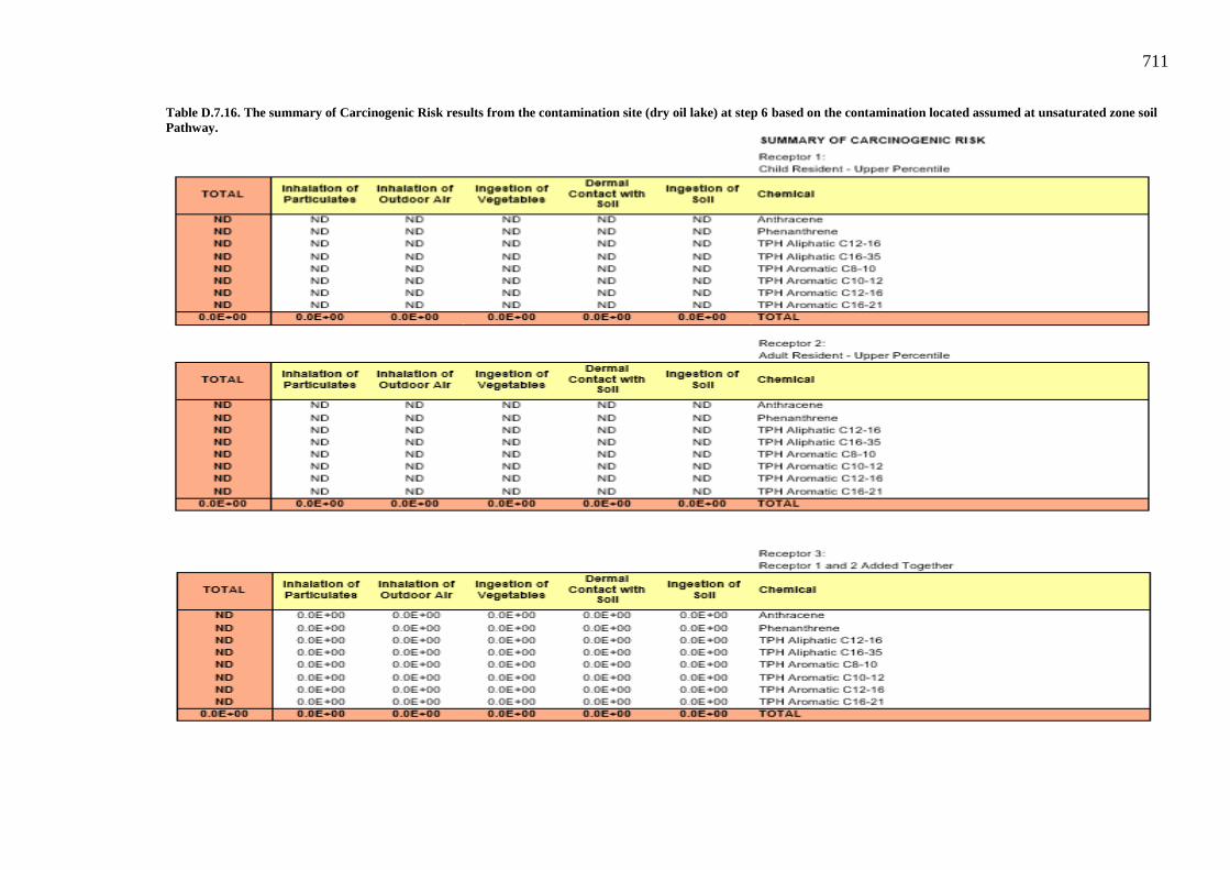
711
Table D.7.16. The summary of Carcinogenic Risk results from the contamination site (dry oil lake) at step 6 based on the contamination located assumed at unsaturated zone soil Pathway.
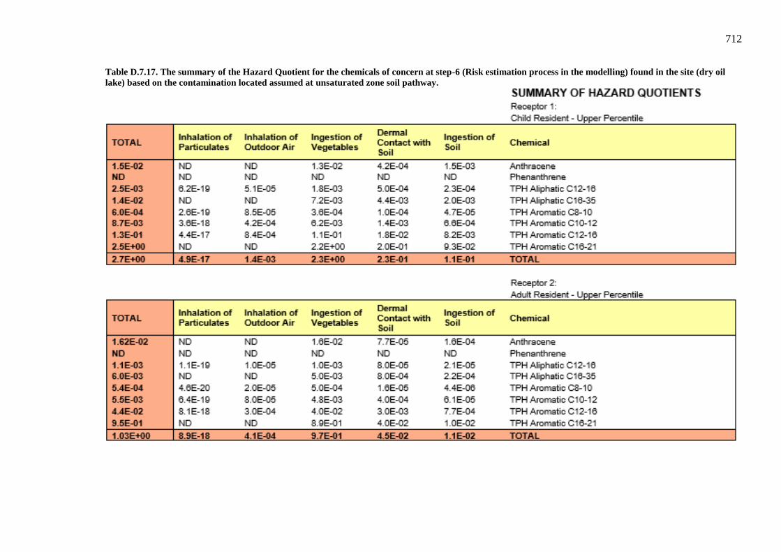
712
Table D.7.17. The summary of the Hazard Quotient for the chemicals of concern at step-6 (Risk estimation process in the modelling) found in the site (dry oil lake) based on the contamination located assumed at unsaturated zone soil pathway.

713
Table D.7.18. The summary of the cumulative clean-up level at step 6 in the modelling
based on the contamination located assumed at unsaturated zone soil pathway.
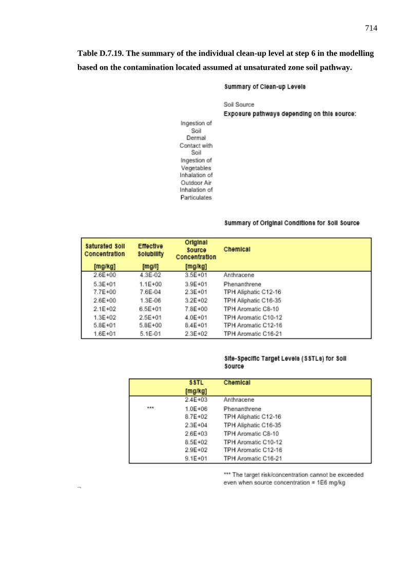
714
Table D.7.19. The summary of the individual clean-up level at step 6 in the modelling
based on the contamination located assumed at unsaturated zone soil pathway.