Comput MechDOI 10.1007/s00466-007-0222-6

ORIGINAL PAPER

A cohesive finite element for quasi-continua

Xiaohu Liu · Shaofan Li · Ni Sheng

Received: 18 May 2007 / Accepted: 20 September 2007© Springer-Verlag 2007

Abstract In this paper, a cohesive finite element method(FEM) is proposed for a quasi-continuum (QC), i.e. a contin-uum model that utilizes the information of underlying atomis-tic microstructures. Most cohesive laws used in conventionalcohesive FEMs are based on either empirical or idealizedconstitutive models that do not accurately reflect the actuallattice structures. The cohesive quasi-continuum finiteelement method, or cohesive QC-FEM in short, is a stepforward in the sense that: (1) the cohesive relation betweeninterface traction and displacement opening is now obtainedbased on atomistic potentials along the interface, rather thanempirical assumptions; (2) it allows the local QC methodto simulate certain inhomogeneous deformation patterns. Tothis end, we introduce an interface or discontinuous Cauchy–Born rule so the interfacial cohesive laws are consistent withthe surface separation kinematics as well as the atomisticallyenriched hyperelasticity of the solid. Therefore, one can sim-ulate inhomogeneous or discontinuous displacement fieldsby using a simple local QC model. A numerical example ofa screw dislocation propagation has been carried out to dem-onstrate the validity, efficiency, and versatility of the method.

Keywords Cohesive laws · Dislocation · Finiteelement method · Nano-mechanics · Quasi-continuum

1 Introduction

The numerical simulation of strong and weak discontinuitieshas been one of the major focuses of computational fail-ure mechanics and engineering reliability analysis in recentyears. Several finite element methods (FEMs) have been

X. Liu · S. Li (B) · N. ShengDepartment of Civil and Environmental Engineering,University of California, Berkeley, CA 94720, USAe-mail: shaofan@berkeley.edu

proposed. Two of the most successful methods are thecohesive FEM proposed by [17], and the so-called extendedfinite element method (X-FEM) proposed by Belytschko et al.[1]. However, most of these methods adopt phenomenolog-ical constitutive relations, which may not be suitable forcomputational nanomechanics. For example, when it comesto simulations of individual dislocation motions, we are notonly interested in how a dislocation moves but also how itaffects the motion of neighboring atoms. The traditional FEbased methods usually have difficulties in capturing thosedetails. An alternative method is molecular dynamics (MD),which has been successfully applied to simulations of thecrack growth. However MD simulates the motion of everysingle atom in the domain, the computational cost can beenormous if the size of the spatial domain of the simulationis up or beyond nanoscale. Today most MD simulations offracture are only limited in nano- or sub-nanoscales.

To build a cost-effective simulation tool, a class ofso-called coarse-grained methods has been proposed. Thesemethods exploit the information at the atomic level but retainsome basic features of continuum mechanics. One of the pop-ular coarse-grained methods is the Quasi-continuum (QC)method, e.g. [16]. A comprehensive review can be found in[12]. There are two versions of the QC method: the localQC and the non-local QC. The local version of QC methodadopts the Cauchy–Born rule, and hence it can only applyto where the local deformation is uniform; while the non-local version was designed to simulate inhomogeneous localdeformations. To achieve that, it needs atomic resolution,and hence it is not really a coarse grain model. Therefore,its computational cost is more expensive and comparable tothat of MD simulations.1

1 In the rest of the paper, when we use the term “QC method,” we referto the local version of QC method, unless indicated otherwise.

123

Comput Mech

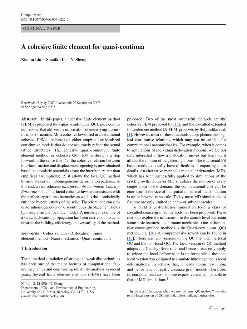
Fig. 1 Illustration of a cohesive surface under finite deformation

A natural question to ask is: Can we simulate non-uniformlocal deformation by using the local version of the QCmethod? The objective of this work is to use the local QCmethod to simulate one particular local inhomogeneousdeformation: strong discontinuity or surface separation. Themain idea of the present approach is to incorporate thecohesive FEM into the local QC framework to form a hybridcohesive QC-FEM method, which can effectively deal withinhomogeneous local deformations, particularly arbitrarystrong discontinuities. In this work, we propose a coarse-grain approach to formulate interfacial cohesive relationssolely based on the information along interfaces at the atomiclevel.

This paper is arranged in the following way. In Sect. 2 weshall present in detail the cohesive QC method, in which anew surface potential based on atomic information is pro-posed. In Sect. 3 we shall discuss the lattice eigenstrainmethod and how to apply the eigenstrain method to cohesiveQC-FEM. To validate the method, we present a simulation ofa screw dislocation propagation in Sect. 4. We then concludethe presentation by making a few remarks in Sect. 5.

2 The cohesive law in a QC

In this section, we consider a solid subjected to an inhomoge-neous deformation that is caused by a displacement discon-tinuity as shown in Fig. 1. In engineering applications, thistype of strong discontinuities is the characterization of frac-ture or dislocations. Initially as a single connected domain,Ω0, the body is broken into two disjointed pieces. In the ref-erential configuration, the fracture surface, or the plane ofdivision, is denoted as S0, and it divides the body into two

halves: Ω0 = B+0

⋃B−

0 . After the deformation ϕ,

ϕ : Ω0 → Ω; (1)

the body arrives at its deformed or current configuration, Ω

(see Fig. 1). We use x denoting the spatial position of a mate-rial point X at the time t , i.e.

x = ϕ(X) = u + X.

Two crack surfaces now move to S+ and S−, respectively.And the two deformed halves are denoted by B+ and B−. Dueto atomic interactions, there will be surface traction betweenS+ and S−. In the rest of the paper, we shall call the fracturesurfaces the cohesive surfaces and the surface traction as thecohesive traction.

The strong form of the governing equations of the prob-lem, i.e. the equations of motion, can be written as:

DIV[P(ϕ)] + ρ0B = ρ0ϕ in B±0 (2)

ϕ = ϕ on ∂ϕ B0 (3)

P(ϕ) · N = t on ∂t B0 (4)

P+ · N + = P− · N − on S±0 (5)

where B is the body force, ρ0 is the mass density in refer-ential configuration. In above equations, the symbol DIV isthe material divergence operator, i.e. ∇X·, N is the normalvector of surfaces including the cohesive surface, t is theprescribed traction on ∂t B0. It is assumed that the traction iscontinuous along the cohesive surface, S0, (5). For domainboundaries, note that

∂φ B0 = ∂φ B+0

⋃∂φ B−

0 and ∂t B0 = ∂t B+0

⋃∂t B−

0 (6)

where ∂ϕ B is the portion of the boundaries where the dis-placements are prescribed, and ∂t B is the portion of theboundaries where the traction is prescribed.

In (2)–(5), P(ϕ) is the first Piola–Kirchhoff stress ten-sor. If we consider the constitutive relation of a hyperelasticmaterial with an elastic energy density W , we may write

P = ∂W

∂Fwhich clearly indicates that P is the function of the deforma-tion map, i.e. P = P(ϕ).

Via standard procedures, we can then derive the Galerkinweak formulation for Eqs. 2–5:∫

B±0

ρ0ϕ · δϕdV +∫

B±0

P(ϕ) · δFdV

=∫

∂t B±0

t · δϕd S +∫

S0

(P(ϕ) · N) · δ(ϕ+ − ϕ−)d S (7)

The last term in the above equation is the virtual work done bythe cohesive traction force across the plane of discontinuity.If we define the jump there as:

123

Comput Mech

∆ = ϕ+ − ϕ− (8)

then we can re-write the last term as:∫

S0

(P(ϕ) · N ) · δ(ϕ+ − ϕ−)d S =∫

S0

tcohe · δ∆d S (9)

where tcohe denotes the cohesive traction. In the continuumcohesive theory e.g. [14], tcohe is defined through the cohe-sive law:

tcohe = ∂W s

∂∆(10)

where W s is the surface energy density.In the continuum cohesive theory, W s is empirical. One

has to take extra effort to choose the surface potential, andthen justify one’s choice. Sometimes we just cannot justifythem to accommodate complex size effects. To be true tothe spirit of coarse graining, one should be able to derivesurface cohesive relations based on the atomic microstruc-ture. However, the difficulty appears to be the discontinuityas a form of local inhomogeneous deformation, which makesthe Cauchy–Born rule break down and hence the coarsegraining scheme. To resolve this issue, we need to modifythe bulk Cauchy–Born rule to incorporate or accommodatekinematics of surface separation. In other words, we need adiscontinuous Cauchy–Born rule, so we can extend the QCformulation to situations where the strong discontinuity orsurface separation is present. Before doing so, we first brieflyreview the procedures of the QC method by deriving the firstPiola–Kirchhoff stress P from atomistic level information.

The basic assumption of the (local) QC method is thatwithin a local region Ωe the deformation gradient F = Fe isconstant. In the setting of FE methods, we can view Ωe asan FE element, most appropriately a triangular element. Theenergy density W e is then defined as:

W e = Ee

Ve(11)

where Ee is the total energy within Ωe and Ve is the volume.Ee can be computed by summing the energies for all atomsin Ωe:

Ee =Ne∑

i=1

Ei (ri1, r i2, . . . , r i Ne ), (12)

and Ne is the total number of atoms in Ωe, Ei is the energyof atom i and

r i j := |xi − x j |, j = 1, 2, . . . , Ne

are the atomic distances between atoms i and j in the currentconfiguration.

For the local QC method to be a coarse-grained approach,a key assumption on local deformation has to be mandated:that is the so-called Cauchy–Born rule (see [2,3]) It states

that, with a constant Fe, all atoms in the underlying latticewithin the same element deform the same way, i.e.

ri j = FeRi j (13)

Here ri j := xi −x j denotes the position vector between atomi and j in the deformed lattice and Ri j := Xi − X j is thedifference of the lattice vectors in the original lattice.

With the Cauchy–Born rule, Ee can be simplified as:

Ee = Ne Ei (ri1, r i2, . . . , r i Ne ) = Ne Ei (Fe) (14)

where i is the index for the i th atom in Ωe, which may rep-resent any atom in Ωe. The energy of the whole domain Ω

is then obtained by summing Ee over all elements:

E =nelem∑

e=1

Ee (15)

where nelem is the total number of elements.We now derive the expression for Pe, the first Piola–

Kirchhoff stress within an element. For simplicity, we onlyconsider the case of two-body interaction. However, the der-ivations can be extended to multi-body interactions withoutdifficulty. From now on, we shall also drop the suffix e inexpressions. One should keep in mind all the quantities arewithin Ωe. We first re-write Ee as:

Ee = Ne Ei (ri1, r i2, . . . , r i Ne ) = Ne

2

Mb∑

j=1

Ei j (ri j (F)) (16)

where Ei j is the potential energy between a pair of atoms,i and j , and 1/2 factor is due to the double counting a pairpotential. Mb is the number of atoms interacting with atomi in the bulk material. In general, Mb Ne if we ignore thefar-field interactions. P can be written as:

P = ∂W e

∂F= Ne

2Ve

Mb∑

j=1

∂ Ei j (r i j )(F)

∂F

= Ne

2Ve

Mb∑

j=1

E ′i j (r

i j )∂r i j (F)

∂F(17)

In the above equation, E ′i j (r

i j ) = d Ei j

dr i jas Ei j is a function

of a single variable r i j . The quantity∂ri j

∂Fcan be computed

as:

∂r i j (F)

∂F= ∂r i j

∂ri j

∂ri j

∂F= ri j ⊗ Ri j

r i j

(18)

In deriving the above expression, (13) is used. The finalexpression of P reads:

P = Ne

2Ve

Mb∑

j=1

E ′i j (r

i j )ri j ⊗ Ri j

r i j(19)

123

Comput Mech

The above derivations are not new, and the objective of thiswork is to use the same philosophy to derive the cohesivetraction law for tcohe based on the information of lattice struc-tures of the solid. To do so, we have to first express the surfaceenergy density in a surface element W es in terms of atomicpotentials. We assume in this paper that W es can be deter-mined solely from the atoms distributed along the pair ofcohesive surfaces. This assumption is similar to the nearest-neighbor-interaction assumption, and it can be lifted at thecost of more involved calculations.

We now consider a pair of opposite crack surface elementSse+ and Sse−. They are the edges of two FE elements. Sincewe only need to formulate W s

e for one of the edges, withoutlosing generality, we shall only consider Sse+. The surfaceenergy density is defined as:

W es = Ees

Aes(20)

where Ees is the total surface energy within the surface ele-ment Sse+, and Aes is the surface area. For Ees , we have:

Ees =Nes∑

i=1

Esi (21)

where Nes is the number of atoms within the surface elementSse+ and

Esi = 1

2

Ms∑

j=1

Ei j (ri js ) (22)

where Ei j (ri js ) are atomistic potentials for surface atoms, r i j

s

are interatomic distances across the interface, i and j are indi-ces for surface atoms only, and Ms is the number of atomson the opposite surface element Sse− that interact with atomi on the surface element Sse+.

Remark 1 1. It assumes that the interface atomic distance,r i j

s = r i js (∆d), is not a function of the local deformation

gradient F, but the nodal displacement separation (thejump) of associated surface elements. For simplicity, inthe rest of paper, we drop the subscript, s , unless it isimportant to indicate it. The nodal displacement sepa-ration is constant within each element. Therefore, thisis essentially an interface Cauchy–Born rule, and weshould further elaborate this point later.

2. In calculating atomistic surface energy potential, as apreliminary study, we only consider the nearest neighborinteraction, and hence the effect of long-range interac-tions such as surface relaxation is neglected. Moreover,this lack of physical realism can be fixed, for instance, byusing a so-called surface Cauchy–Born approach ([15]).In fact, the procedure proposed by [15] is one way tocalculate atomic surface potentials. It may be possiblethat we can still use the proposed approach, but choose

an appropriate surface potential, ESi j (r

i j ) = Ei j (r i j ),to capture some of surface effects. In fact, there havebeen some specific surface potentials proposed in theliterature, e.g. [7].

Similar to what we did for element interior, we adopt thefollowing QC approximation:

Ees ≈ Nes Esi (23)

where Nes is the number of atoms on the surface elementSse+. This approximation means that we assume that allatoms in Sse+ to have the same surface energy.

To derive the expression for the cohesive traction, we con-sider a FE discretization of the domain. The FE approxima-tion of the displacement field is given by:

u(X) = N(X)d (24)

where

N(X) = [Ni j (X)]ndim×ndof

is the shape function matrix, ndim is the number of dimen-sion of space, ndof is the number of degrees of freedom, andd is the nodal displacement vector. In the following, we shallmix the tensor notation with matrix notation in the deriva-tion, because some of the matrices here may be viewed assecond-order tensors.

Consider a separation, or a jump, between a pair of cohe-sive surfaces as shown in Fig. 2. The jump can also bedescribed by FEM interpolation:

∆ = Ns(X)∆d (25)

where Ns(X) is the matrix of edge shape functions. The nodaljump vector ∆d is defined by:

∆d = d+ − d− (26)

where d+ and d− are nodal displacement vectors on S+ andS−, respectively. Moreover, the following relationship holds:

d+ = 〈d〉 + 1

2∆d (27)

d− = 〈d〉 − 1

2∆d (28)

where 〈d〉 = 12 (d+ + d−). So,

∂d+

∂∆d= 1

2(29)

∂d−

∂∆d= −1

2(30)

123

Comput Mech

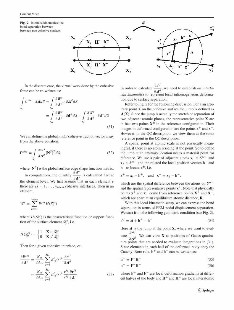
Fig. 2 Interface kinematics: thebond separation betweenbetween two cohesive surfaces

In the discrete case, the virtual work done by the cohesiveforce can be re-written as:∫

S0

tcohe · δ∆d S =∫

S0

∂W s

∂∆d· δ∆dd S

=∫

S0

∂W s

∂∆d· δd+d S −

∫

S0

∂W s

∂∆d· δd−d S

(31)

We can define the global nodal cohesive traction vector arrayfrom the above equation:

fcohe =∫

S0

∂W s

∂∆d[NS]T d S (32)

where [NS] is the global surface edge shape function matrix.

In computations, the quantity∂W s

∂∆dis calculated first at

the element level. We first assume that in each element ethere are es = 1, . . . , nselem cohesive interfaces. Then in anelement,

W s =nselem∑

es=1

W es H(Ses0 )

where H(Ses0 ) is the characteristic function or support func-

tion of the surface element Ses0 , i.e.

H(Ses0 ) =

1 X ∈ Ses

00 X ∈ Ses

0

Then for a given cohesive interface, es,

∂W es

∂∆d= Nes

2Aes

Ms∑

j=1

E ′i j (r

i j )∂r i j

∂∆d

= Nse

2Aes

Ms∑

j=1

E ′i j (r

i j )ri j

r i j

∂ri j

∂∆d(33)

In order to calculate∂ri j

∂∆d, we need to establish an interfa-

cial kinematics to represent local inhomogeneous deforma-tion due to surface separation.

Refer to Fig. 2 for the following discussion. For a an arbi-trary point X on the cohesive surface the jump is defined as∆(X). Since the jump is actually the stretch or separation oftwo adjacent atomic planes, the representative point X arein fact two points X± in the reference configuration. Theirimages in deformed configuration are the points x+ and x−.However, in the QC description, we view them as the samereference point in the QC description.

A spatial point at atomic scale is not physically mean-ingful, if there is no atom residing at the point. So to definethe jump at an arbitrary location needs a material point forreference. We use a pair of adjacent atoms xi ∈ Sse+ andx j ∈ Sse− and the related the local position vectors h+ andh− to locate x±, i.e.

x+ = xi − h+, and x− = x j − h−.

which are the spatial difference between the atoms on Sse±and the spatial representative points x±. Note that physicallypoints x+ and x− come from reference points X+ and X−,which are apart at an equilibrium atomic distance, R.

With this local kinematic setup, we can express the bondseparation in terms of FEM nodal displacement separation.We start from the following geometric condition (see Fig. 2),

ri j = ∆ + h+ − h− (34)

Here ∆ is the jump at the point X, where we want to eval-

uate∂ri j

∂∆d. We can view X as positions of Gauss quadra-

ture points that are needed to evaluate integrations in (31).Since elements in each half of the deformed body obey theCauchy–Born rule, h+ and h− can be written as:

h+ = F+H+ (35)

h− = F−H− (36)

where F+ and F− are local deformation gradients at differ-ent halves of the body and H+ and H− are local interatomic

123

Comput Mech

position vectors in the undeformed configuration correspond-ing to the spatial position vectors, h±. The above equationscan then be re-written as:

h± = F±H± =(

1 + u±,X

)· H± = 1 · H± + B±

· (d± ⊗ H±)(37)

where B± are two third-order tensors whose components aredefined as

B±i j A = N±

i j,A := ∂

∂ X AN±

i j (38)

Here the capital letter A denotes the index of the referencecoordinates.

Considering the interfacial kinematic relation shown inFig. 2, we have the following geometric relations at an arbi-trary point (a pair of points) of the interface,

∆ = ri j + (h− − h+) = (xi − x j ) + (h− − h+)

= F+ · Xi − F− · X j + F− · H− − F+ · H+

= F+ · X+ − F− · X− (39)

Define

X := 1

2

(X+ + X−)

, and ∆0 := 1

2

(X+ − X−)

. (40)

We have the interface Cauchy–Born rule as follows:

∆ = (F+ + F−) · ∆0 + (

F+ − F−) · X (41)

Now, we can calculate the derivative of ri j with respectto element nodal jump vector, ∆d ,

∂ri j

∂∆d= ∂∆

∂∆d+ ∂h+

∂∆d− ∂h−

∂∆d

= Ns + ∂h+

∂d+∂d+

∂∆d− ∂h−

∂d−∂d−

∂∆d

= Ns + 1

2B+H+ − 1

2B−H− (42)

The final expression of∂W es

∂∆dreads:

∂W es

∂∆d= Nes

2Aes

Ms∑

j=1

E′i j (r

i j )∂r i j

∂∆d

= Nes

2Aes

Ms∑

j=1

E′i j (r

i j )1

r i j

(

ri j · Ns

+ 1

2ri j · B+H+ − 1

2ri j · B−H−

)

(43)

The matrix form of the above equation is:

∂W es

∂∆d= Nes

2Aes

Ms∑

j=1

E ′i j (r

i j )

r i j

(

[NsT ]ri j + 1

2[B+H+]T ri j

−1

2[B−H−]T ri j

)

(44)

The components of matrices B±H± are:

[B±H±]i j = N±i j,A H±

A (45)

where N±i j are components of N. The force vector fcohe can

be obtained by integrating∂W s

∂∆d.

Remark 2 From (43), we observe that when B+H+ =B−H−, the expression of nodal traction vector will reduceto:

fcohe = nelemA

e=1

nselemA

es=1

∫

Ses0

Nes

2Aes

Ms∑

j=1

E ′i j (r

i j )

r i jNsT ri j d S (46)

This corresponds to the case when the deformed atomic posi-tion vectors are the same on S+ and S−. In the above equationA is the element assembly operator for both bulk elementsand surface elements [6]. Since in each element there maybe several cohesive interfaces, i.e. es = 1, . . . , nselem, so wehave used double assembly operators as a two-loop assemblyfor each bulk element and for each surface element within abulk element.

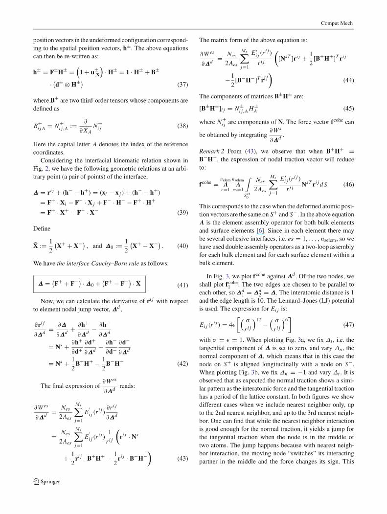
In Fig. 3, we plot fcohe against ∆d . Of the two nodes, weshall plot fcohe

1 . The two edges are chosen to be parallel toeach other, so ∆d

1 = ∆d2 = ∆. The interatomic distance is 1

and the edge length is 10. The Lennard–Jones (LJ) potentialis used. The expression for Ei j is:

Ei j (ri j ) = 4ε

[( σ

r i j

)12 −( σ

r i j

)6]

(47)

with σ = ε = 1. When plotting Fig. 3a, we fix ∆t , i.e. thetangential component of ∆ is set to zero, and vary ∆n , thenormal component of ∆, which means that in this case thenode on S+ is aligned longitudinally with a node on S−.When plotting Fig. 3b, we fix ∆n = −1 and vary ∆t . It isobserved that as expected the normal traction shows a simi-lar pattern as the interatomic force and the tangential tractionhas a period of the lattice constant. In both figures we showdifferent cases when we include nearest neighbor only, upto the 2nd nearest neighbor, and up to the 3rd nearest neigh-bor. One can find that while the nearest neighbor interactionis good enough for the normal traction, it yields a jump forthe tangential traction when the node is in the middle oftwo atoms. The jump happens because with nearest neigh-bor interaction, the moving node “switches” its interactingpartner in the middle and the force changes its sign. This

123

Comput Mech

Fig. 3 Cohesive traction as a function of distances. a Normal traction, and b Tangential traction

artificial effect is eliminated when the 2nd nearest neighborinteraction is considered. [17] provided a similarly shapedcohesive relation by using an empirical surface potential.

The other terms in the weak form can be treated by stan-dard FE procedures, and we choose not to show the deriva-tion. The final expression is:

Md + f int (d) − fcohe(d) = fext (48)

where:

M = nelemA

e=1

∫

Be0

ρ0NeT NedV (49)

f int = nelemA

e=1

∫

Be0

BeT Pe(d)dV (50)

fext = nelemA

e=1

∫

∂t B±e0

NeT ted S (51)

and Be is the matrix for element shape function gradient.

3 Application in simulation of dislocation propagations

In general, a line defect like the dislocation will naturallyoccur when a crystal is under external stress. When the con-figurational force i.e. the Peach-Koehler force is greater thanthe lattice friction force i.e. the Peierls force under specifictemperature, the dislocation will then move.

There are many techniques in Molecular Dynamics tosimulate dislocation motions. To study the motion of a sin-gle dislocation, there are even analytical solutions as well assemi-analytical solutions available for Molecular Dynamicsor Lattice Dynamics. The analytical approach was first devel-oped for Lattice Statics by [11], and it was then extendedby [13] to Lattice Dynamics. In analytical solution proce-dure, the dislocation is preconfigured, and the Lattice Green’sFunction technique is often used to solve dislocation motions.This technique can only be employed in an infinite lattice

space. For finite lattice spaces, the semi-analytical solutionis useful. In the semi-analytical solution, the dislocation ispreconfigured, i.e. the defect field is initially prescribed byimposing a so-called eigenstrain field, the MD simulationthen takes care of the rest based on the equation of motion orthe interatomic force relation. This type of solutions is verysuitable to serve as the benchmark solution for numericalsimulations because of their analytical nature.

Here, we briefly outline this method first, and then com-pare its results to that of the proposed cohesive QC-FEMcomputation. We consider a general 3D lattice, and we limitourselves to the case of harmonic approximation. For an atom, the equation of motion reads:

ma u() = −∑

′φ(, ′)u(′) (52)

where ma is the mass, φ(, ′) is the coefficient of a constantmatrix that is related to the force between atoms and ′.Furthermore, we have the following expression:

u(′) − u() = [β(, ′) + β∗(, ′)

]x(′) (53)

where x(′) = x(′) − x(). β(, ′) and β∗(, ′) arethe elastic distortion and the eigen-distortion between and′, respectively. We have a non-zero eigen-distortion if thedomain is subject to inelastic deformations like dislocations.

Remark 3 The symmetric part of (53) is analogous to thefollowing equation in the theory for continuum:

1

2

(∇u + (∇u)T

)= εe + ε∗ (54)

where εe is the elastic strain and ε∗ is the eigenstrain.

Mura [13] showed that with (53), the MD equation ofmotion takes a new form:

ma u() = −∑

′φ(, ′)u(′)+

∑

′φ(, ′)β∗(, ′)x(′)

(55)

123

Comput Mech

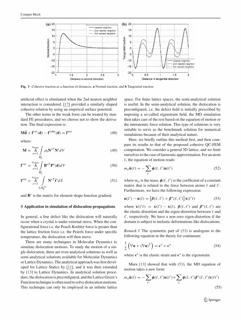
Fig. 4 A plane view of the cubic lattice

The extra term on the right hand side (55) is a fictitious bodyforce due to eigen-distortions which are caused by defects.

Now let us consider the a specific type of defects: a screwdislocation. We shall use it as an example to illustrate howthe value of the dislocation force is calculated by eigen-strains. The problem setting is shown in Fig. 4. We consider acubic lattice with nearest neighbor interactions. An index pair(m, n) is used to denote a particular atom. The interatomicdistance is h. The screw dislocation is in the x3-direction andis moving in the x1-direction with a constant speed v. As aresult, we only need to consider x3-direction displacements.

Let us assume the dislocation has propagated to the col-umn of atoms with m = m0. Then for all pair of atoms(k+0.5,−0.5) and (k+0.5, 0.5), k ∈ (−∞, m0], the inelas-tic displacement is h, i.e. the amount of dislocation. So wehave:

β∗(, ′)x2(′) = h (56)

Since x2(′) = h, we have β∗ = 1 in this case. Thus it is

easy to obtain the following equation of motion [8]:

mau3(m, n) = A [u3(m + 1, n) + u3(m − 1, n)]

+B [u3(m, n + 1) + u3(m, n − 1)]

−2(A + B)u3(m, n)

+Bhm0∑

k=−∞

(δm,k+0.5δn,0.5−δm,k−0.5δn,−0.5

)

(57)

where A and B are force constants in x1x3- and x2x3-directions, respectively. By applying the above procedure to

Molecular Dynamics, we can simulate dislocation motionsin a lattice.

In our cohesive QC-FEM approach, the dislocation forces±Bh are treated as prescribed forces. For FE nodes thatare at and behind the dislocation front, we apply the dis-location forces. They appear in the external force vectorfext. To propagate the dislocation, we adopt the so-calledquarter-jump rule [11]. Let x+ and x− be two atoms locatingat the opposite sides of the dislocation plane. If the followingcondition is satisfied:

∆ = u3(x+) − u3(x−) > 0.25h (58)

we consider the dislocation having passed through this point,and we start to apply dislocation forces to the adjacent pairof nodes.

4 A numerical example

In this section, we present the numerical simulation of apropagating screw dislocation using the cohesive QC-FEMapproach. We simulate a domain with a dimension of[−50, 50] × [−50, 50]. The interatomic spacing is chosento be 1. The force constants are A = B = 1. The dislocationinitiates at the left side of the domain. We performed two sim-ulations. One has 200 linear triangle elements and the otherone has 800 elements. The cohesive surface is chosen to bethe x = 0 plane. For comparison purpose, we also simulatethe problem with Molecular Dynamics(MD). The equationof motion is (57). There are total of 10201 atoms.

For time integration, Verlet algorithm is used in both cases.The time steps are 0.3162 and 0.1581 for the cohesiveQC-FEM simulations and 0.0316 for the MD simulation.

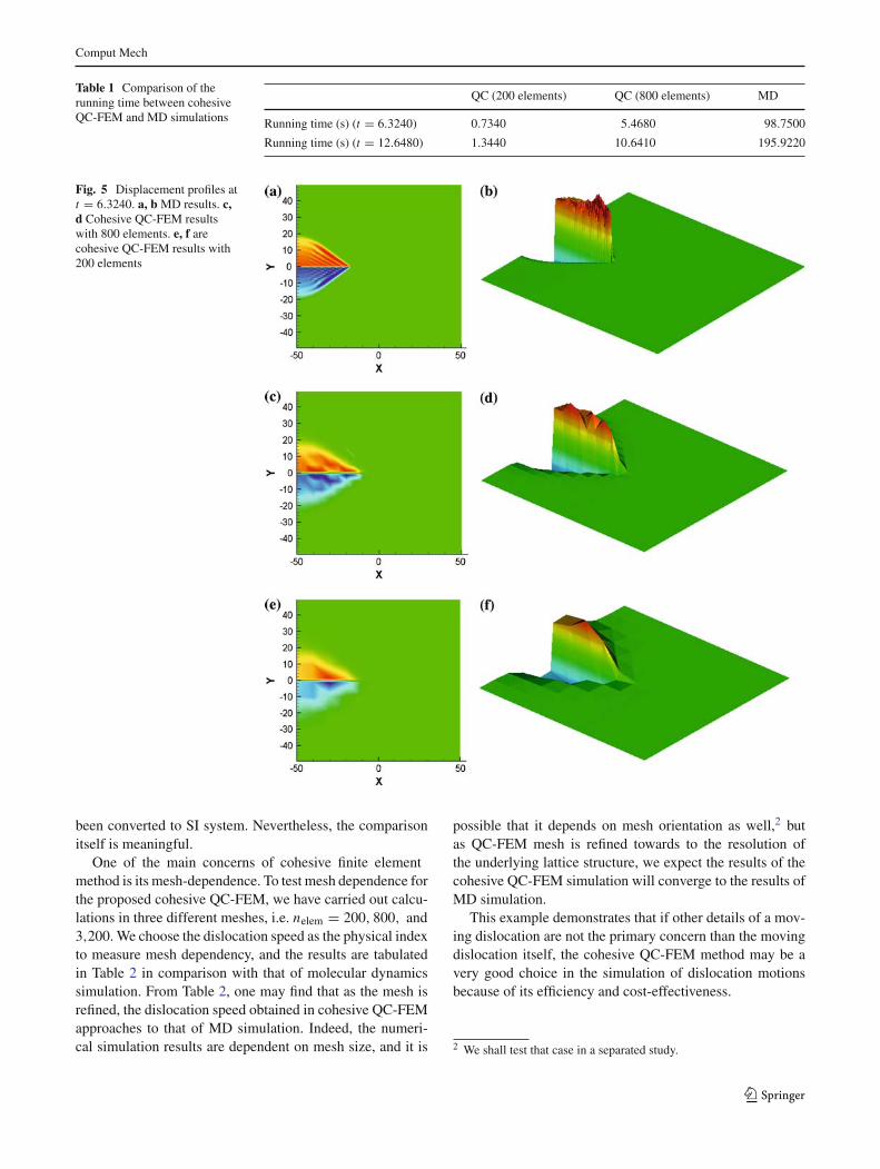
The simulations were carried out in a PC with an 1.8 GHzAMD64 processor. The different CPU times used in com-putations of the same problem but with different modelingsand different discretizations are tabulated in Table 1. FromTable 1, one may find that the cohesive QC-FEM simulationhas far less computational cost than that of the MD simula-tion: the 200-element simulation and the 800-element sim-ulation take 0.7 and 5.5% of the time of MD simulation,respectively. At the same time, the cohesive QC-FEM sim-ulation still has a very good accuracy. Shown in Figs. 5 and6 are the displacement profiles at time t = 6.3240 and t =12.6480. We can see the cohesive QC-FEM simulation cap-tures the main feature of the problem. Table 2 shows thedislocation speed (computed by the distance that the disloca-tion front has traveled by time). We observe that dislocationspeed is close between the results obtained by the cohesiveQC-FEM and by MD. It should be noted that since the com-putation is done for fictitious materials the unit for the dis-location speed here is used a computational unit that has not

123

Comput Mech

Table 1 Comparison of therunning time between cohesiveQC-FEM and MD simulations

QC (200 elements) QC (800 elements) MD

Running time (s) (t = 6.3240) 0.7340 5.4680 98.7500

Running time (s) (t = 12.6480) 1.3440 10.6410 195.9220

Fig. 5 Displacement profiles att = 6.3240. a, b MD results. c,d Cohesive QC-FEM resultswith 800 elements. e, f arecohesive QC-FEM results with200 elements

been converted to SI system. Nevertheless, the comparisonitself is meaningful.

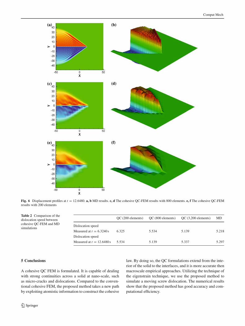
One of the main concerns of cohesive finite elementmethod is its mesh-dependence. To test mesh dependence forthe proposed cohesive QC-FEM, we have carried out calcu-lations in three different meshes, i.e. nelem = 200, 800, and3,200. We choose the dislocation speed as the physical indexto measure mesh dependency, and the results are tabulatedin Table 2 in comparison with that of molecular dynamicssimulation. From Table 2, one may find that as the mesh isrefined, the dislocation speed obtained in cohesive QC-FEMapproaches to that of MD simulation. Indeed, the numeri-cal simulation results are dependent on mesh size, and it is

possible that it depends on mesh orientation as well,2 butas QC-FEM mesh is refined towards to the resolution ofthe underlying lattice structure, we expect the results of thecohesive QC-FEM simulation will converge to the results ofMD simulation.

This example demonstrates that if other details of a mov-ing dislocation are not the primary concern than the movingdislocation itself, the cohesive QC-FEM method may be avery good choice in the simulation of dislocation motionsbecause of its efficiency and cost-effectiveness.

2 We shall test that case in a separated study.

123

Comput Mech

Fig. 6 Displacement profiles at t = 12.6480. a, b MD results. c, d The cohesive QC-FEM results with 800 elements. e, f The cohesive QC-FEMresults with 200 elements

Table 2 Comparison of thedislocation speed betweencohesive QC-FEM and MDsimulations

QC (200 elements) QC (800 elements) QC (3,200 elements) MD

Dislocation speed

Measured at t = 6.3240 s 6.325 5.534 5.139 5.218

Dislocation speed

Measured at t = 12.6480 s 5.534 5.139 5.337 5.297

5 Conclusions

A cohesive QC FEM is formulated. It is capable of dealingwith strong continuities across a solid at nano-scale, suchas micro-cracks and dislocations. Compared to the conven-tional cohesive FEM, the proposed method takes a new pathby exploiting atomistic information to construct the cohesive

law. By doing so, the QC formulations extend from the inte-rior of the solid to the interfaces, and it is more accurate thenmacroscale empirical approaches. Utilizing the technique ofthe eigenstrain technique, we use the proposed method tosimulate a moving screw dislocation. The numerical resultsshow that the proposed method has good accuracy and com-putational efficiency.

123

Comput Mech

We are currently working on extending the method to3D problems and problems involving with multiple disloca-tions. By using the atomic information, the proposed methodcan also be incorporated into a multiscale scheme with themolecular dynamics method. This has recently been doneby the present authors [10]. A multiscale simulation of amoving screw dislocation has been carried out there, whichallows a dislocation passing through different scales. In short,we believed that the proposed method provides an effectivecoarse grained approach to simulate fracture and dislocationmotions.

Acknowledgments The authors acknowledge the fact that Mr.Ashutosh Agrawal participated the early phase of this work. We thankhim for his suggestion of using a spring model to represent surfacecohesive law and his early involvement in computer code development.This work is supported by a grant from NSF (Grant no. CMS-0239130),which is greatly appreciated.

References

1. Belytschko T, Moes N, Usui S, Parimi C (2001) Arbitrary discon-tinuities in finite elements. Int J Numer Methods Eng 50:993–1013

2. Born M (1915) Dynamik der Krystallgitter. Teubner, Leipzid/Berlin

3. Born M, Huang K (1954) Dynamical theory of crystal lattices.Clarendon Press, Oxford

4. Callari C, Armero F (2004) Analysis and numerical simulation ofstrong discontinuities in finite strain poroplasticity. Comput Meth-ods Appl Mech Eng 193:2941–2986

5. Dolbow J (1999) An extended finite element method with discon-tinuous enrichment for applied mechanics. PhD Thesis, Northwest-ern University

6. Hughes TJR (1987) The finite element method: linear static anddynamic finite element analysis. Prentice Hall, Englewood Cliffs

7. Ibach H (1997) The role of surface stress in reconstruction, epitax-ial growth and stabilization of mesoscopic structures. Surf Sci Rep29:193–263

8. King KC, Mura T (1991) The eigenstrain method for small defectsin a lattice. J Phys Chem Solids 52:1019–1030

9. Klein P, Gao H (1998) Crack nucleation and growth as strain local-ization in a virtual bond continuum. Eng Fract Mech 61:21–48

10. Li S, Liu X, Agrawal A, To AC (2006) The perfectly matchedmultiscale simulations for discrete systems: Extension to multipledimensions. Phys Rev B 74:045418

11. Maradudin A (1958) Screw dislocations and discrete elastic theory.J Phys Chem Solids 9:1–20

12. Miller RE, Tadmor EB (2002) The quasicontinuum method: over-view, applications and current directions. J Comput Aided Materi-als Des 9:203–239

13. Mura T (1977) Eigenstrains in lattice theory. University ofWaterloo Press, Waterloo

14. Ortiz M, Pandolfi A (1999) Finite-deformation irreversible cohe-sive elements for three-dimensional crack-propagation analysis. IntJ Numer Methods Eng 44:1267–1282

15. Park H, Klein P, Wagner G (2006) A surface Cauchy–Born modelfor nanoscale materials. Int J Numer Methods Eng 68:1072–1095

16. Tadmor E, Ortiz M, Phillips R (1996) Quasicontinuum analysis ofdefects in solids. Philos Mag A 73:1529–1563

17. Xu X-P, Needleman A (1994) Numerical simulations of fast crackgrowth in brittle solids. J Mech Phys Solids 42:1397–1434

123