arX

iv:a

stro

-ph/

0408

461v

1 2

5 A

ug 2

004

Noise storm continua: power estimates for electron acceleration

Prasad Subramanian∗

Inter-University Centre for Astronomy and Astrophysics, P.O. Bag 4,

Ganeshkhind, Pune - 411007, India.

Peter A. Becker† ‡

Center for Earth Observing and Space Research,

School of Computational Sciences,

George Mason University, Fairfax, VA 22030, USA

Abstract. We use a generic stochastic acceleration formalism to examine thepower Lin (erg s−1) input to nonthermal electrons that cause noise storm continuumemission. The analytical approach includes the derivation of the Green’s functionfor a general second-order Fermi process, and its application to obtain the particularsolution for the nonthermal electron distribution resulting from the acceleration ofa Maxwellian source in the corona. We compare Lin with the power Lout observedin noise storm radiation. Using typical values for the various parameters, we findthat Lin ∼ 1023−26 erg s−1, yielding an efficiency estimate η ≡ Lout/Lin in the range10−10

∼< η ∼

< 10−6 for this nonthermal acceleration/radiation process. These resultsreflect the efficiency of the overall process, starting from electron acceleration andculminating in the observed noise storm emission.

Keywords:

1. Introduction

Solar noise storms are a very well studied phenomenon. They occurmostly at meter wavelengths, and comprise a long-lasting (1 hr – severaldays) broadband (δf/f ∼ 100%) component together with narrowband(δf/f ∼ few %) spiky bursts that last from 0.1 – 1 s. Elgaroy (1997)gives a thorough observational review of noise storms. Malik & Mercier(1996) present a comprehensive study of noise storms observed with theNancay Radioheliograph (NRH). Klein (1998) presents a recent reviewof the role of suprathermal electrons in the solar corona that includesa broad discussion of the noise storm phenomenon.

In this study, we confine our attention primarily to type I noisestorm continua, rather than the sporadic type I bursts, because weare interested in examining the basic energetics of the electron accel-

∗ e-mail: psubrama@iucaa.ernet.in† e-mail: pbecker@gmu.edu‡ also Dept. of Physics and Astronomy, George Mason University, Fairfax, VA

22030, USA

c© 2008 Kluwer Academic Publishers. Printed in the Netherlands.

noise22.tex; 2/02/2008; 12:51; p.1

2 Subramanian & Becker

eration processes responsible for producing the quasi-continuous radioemission.

Most theories of type I phenomena invoke nonthermal electrons as acrucial ingredient in producing the observed radiation. It is recognizedthat the nonthermal electrons that are involved in generating the noisestorm continua are probably accelerated in closed coronal loops aboveactive regions. Noise storm continua are sometimes accompanied bycoincident (thermal) soft X-ray brightenings (e.g., Raulin & Klein 1994;Krucker et al. 1995), which are also signatures of coronal magneticfield evolution. When this occurs, it is clear that the electrons in thetail of the thermal distribution that produce the accompanying soft X-radiation cannot also produce the observed radio noise storm emissionfor more than a few minutes. This is inconsistent with the fact that noisestorms are observed to persist for several hours to days (e.g., Raulin& Klein 1994; Malik & Mercier 1996 also present similar arguments).Since the X-ray emitting regions are typically situated at least one scaleheight below the layer in the corona where the noise storms originate,the two associated electron distributions cannot be co-spatial. Crosbyet al. (1996) find that deka-keV X-ray emission is often observed to-wards the beginning of noise storms. The electrons producing this X-rayemission are energetic enough to power the noise storm simultaneously,and they could be transported to the noise storm emitting region eitherby turbulent diffusion or by direct transport along connecting magneticfield lines. However, the duration of the noise storm is much longer thanthe X-ray emission, and consequently continual electron acceleration isrequired. The acceleration is probably triggered by the same processesthat give rise to the X-ray brightenings accompanying the onset of thenoise storms.

Clearly an underlying acceleration mechanism is required in orderto produce the nonthermal electron distribution implied by the noisestorm emission. However, very little attention has been focused on thisproblem in the previous literature. The majority of the current theoriessimply assume that nonthermal electrons are present, and focus mostof their attention on examining the wave-wave interaction processesthrough which observable radio emission is ultimately produced. It isfairly well established that noise storms are intimately connected withthe temporal variation of the magnetic fields via the process of coronalevolution (e.g., Brueckner 1983; Stewart et al. 1986; Raulin & Klein1994; Willson et al. 1997; Bentley et al. 2000). However, the precisephysical processes that link the magnetic field evolution to the presenceof nonthermal electrons is unclear. Spicer et al. (1981) adopted a specificdriver model in order to examine the basic energetics of the processleading to type I bursts. Benz & Wentzel (1981) developed a similar

noise22.tex; 2/02/2008; 12:51; p.2

Noise storm continua 3

treatment that is also valid for type I bursts. The basic driver in both ofthese pictures is the process of coronal evolution, which causes magneticfields to emerge into the corona and drive microinstabilities that spawnlow-frequency turbulence. This turbulence in turn resonates with theelectrons and stochastically accelerates them to form a nonthermal tail.

Our goal here is to develop a model-independent approach to theestimation of the noise storm energetics that avoids focusing on aspecific mechanism for accelerating the electrons. Instead, we prescribea generic second-order (stochastic) Fermi mechanism. Electrons fromthe tail of the thermal distribution are injected into the accelerationprocess, forming a nonthermal distribution. Only electrons above acritical energy in the tail of the thermal distribution are subjected tonet acceleration; the rest remain thermal due to collisions. The basicparameters of the acceleration mechanism are constrained as follows.First we borrow from the literature estimates of the nonthermal elec-tron fraction needed to produce the observed noise storm continua. Bycombining this estimate with approximate expressions for the domi-nant loss timescales influencing the electrons, we derive an estimatefor the power that drives the electron acceleration process. This yieldsan approximate determination of the efficiency of the process startingfrom nonthermal electron acceleration and culminating in the observednoise storm emission. The efficiency so obtained is a relatively well-defined quantity that provides a general, model-independent constrainton the acceleration/radiation mechanisms, which in turn serves as auseful guide in the subsequent development of more detailed models.Furthermore, we expect that a good understanding of the efficiency ofelectron acceleration in the context of the solar corona will also provideuseful insights into similar phenomena occurring in other astrophysicalenvironments.

2. Electron acceleration

2.1. Why are nonthermal electrons important?

There is considerable observational evidence for the presence of non-thermal electrons in nonflaring regions of the solar corona (e.g., Klein1998). The high brightness temperatures and significant positive spec-tral slopes in multi-frequency observations of noise storms stronglysuggest an underlying nonthermal electron population (e.g., Thejappa& Kundu 1991; Sundaram & Subramanian 2004). An anisotropy invelocity or physical space causes these nonthermal electrons to spon-taneously emit Langmuir/upper hybrid waves (e.g., Robinson 1978;

noise22.tex; 2/02/2008; 12:51; p.3

4 Subramanian & Becker

Wentzel 1985), which can coalesce with a suitable low-frequency wavepopulation to produce the observed electromagnetic emission.

Melrose (1980) argues that low-frequency turbulence (including ion-acoustic, lower-hybrid, or a variety of other waves) will be generatedas a natural product of coronal heating. Thejappa (1991) considerslower-hybrid waves excited by protons (as in Wentzel 1986) or bya series of weak shocks (as in Spicer et al. 1981) as candidates forthe low-frequency wave population. Benz & Wentzel (1981) investigatethe possibility that the turbulence is composed of ion-acoustic wavesexcited by evolving magnetic fields in the corona.

While most of the theories for noise storm continua do not specifythe source of the nonthermal electrons powering the observed emission,Benz & Wentzel (1981) propose that these electrons are leftover par-ticles from the population that produced the previous type I bursts.However, Krucker et al. (1995) note that the type I continuum andbursts are spatially separated. Furthermore, Malik & Mercier (1996)pointed out that solar noise storms are often not bursty in the be-ginning, and the continuum exists alone. These observational resultscontradict Benz & Wentzel’s (1981) picture for the production of thenonthermal electrons. On the other hand, the model proposed by Spiceret al. (1981) for type I bursts considers the electrons to be acceleratedvia the modified two-stream instability, which in turn is spawned byrandom weak shocks caused by the emerging magnetic flux. However,this suggestion is contradicted by the work of Krucker et al. (1995).

Although there is currently no theoretical consensus regarding thefundamental mechanism powering type I phenomena, there is no ques-tion that nonthermal electrons are responsible for the observed emis-sion. This situation leads us to suggest that a careful examination ofthe energy budget and the associated constraints on the efficiency ofthe acceleration process may provide the best route towards enhancedphysical understanding.

2.2. Energy loss mechanisms

It is expected that the electron momentum distribution, f , will haveessentially a two-part structure, comprising a thermal component alongwith a nonthermal, high-energy (but still nonrelativistic) electron “tail”that is responsible for producing the noise storm emission. In view of theconsiderable uncertainty surrounding the precise physical mechanismthat results in the formation of the nonthermal portion of the electrondistribution, we shall work in terms of a generic, stochastic (second-order) Fermi process. The total electron number density, ne, includingboth thermal and nonthermal particles, is related to the momentum

noise22.tex; 2/02/2008; 12:51; p.4

Noise storm continua 5

distribution f via

ne (cm−3) =

∫ ∞

0p2 f dp , (1)

where p is the electron momentum. The associated total electron energydensity is given by

Ue (erg cm−3) =

∫ ∞

0ǫ p2 f dp =

1

2me

∫ ∞

0p4 f dp , (2)

where me is the electron mass and ǫ = p2/(2me) is the electron kineticenergy. In the present application, we are mainly interested in thenonthermal electrons, which are picked up from the thermal populationand subsequently accelerated to high energies.

At marginal stability, the loss timescale due to the emission ofLangmuir waves by electrons is similar to the Coulomb loss timescale(Melrose 1980). The mean Coulomb energy loss rate for nonthermalelectrons with energy ǫ colliding with ambient electrons and protons ina fully-ionized hydrogen plasma is given in cgs units by (e.g., Brown1972b)

⟨

dǫ

dt

⟩∣

∣

∣

∣

loss=

1.57 × 10−23 Λne

ǫ1/2

(

1 +me

mp

)

, (3)

where Λ is the Coulomb logarithm and mp is the proton mass. The firstand second terms in parentheses on the right-hand side of equation (3)refer to electron-electron and electron-proton collisions, respectively.The factor of me/mp clearly indicates that the cooling rate due toelectron-proton bremsstrahlung is negligible compared with the effectof electron-electron collisions. Ignoring the factor of me/mp in equa-tion (3), we find that the characteristic timescale for Coulomb losses isgiven by

tloss ≡ ǫ

⟨

dǫ

dt

⟩−1∣∣

∣

∣

loss=

6.37 × 1022 ǫ3/2

Λne(4)

in cgs units.

2.3. Stochastic acceleration of electrons

For low electron energies, ǫ ∼< kT , collisions between electrons are ex-pected to efficiently maintain a Maxwellian distribution. However, weshall demonstrate below that for electron energies exceeding the criticalenergy ǫc, stochastic acceleration dominates over collisional losses onaverage (see eq. [10]). In this situation, the high-energy tail of theelectron distribution function is governed by a rather simple transportequation that describes the diffusion of electrons in momentum space

noise22.tex; 2/02/2008; 12:51; p.5

6 Subramanian & Becker

due to collisions with magnetic scattering centers. The time evolutionof the Green’s function for this process, fG , is described by (e.g., Becker1992; Schlickeiser 2002)

∂fG

∂t=

1

p2

∂

∂p

(

p2 D ∂fG

∂p

)

+N0 δ(p − p0)

p20

− fG

τ, (5)

where D is the (as yet unspecified) diffusion coefficient in momentumspace and τ is the mean residence time for electrons in the accelerationregion. The source term in equation (5) corresponds to the injection intothe acceleration region of N0 particles per unit volume per unit time,each with momentum p0. Although we do not explicitly include lossesdue to the emission of Langmuir/upper hybrid waves by the acceleratedelectrons, it is expected that these waves will be generated as a naturalconsequence of the spatial anisotropy of the electron distribution (e.g.,Thejappa 1991). We will demonstrate below that our neglect of energylosses due to Coulomb collisions and the emission of Langmuir/upperhybrid waves is reasonable for the nonthermal electrons treated byequation (5). Note that in writing equation (5), we have ignored spatialtransport so as to avoid unnecessary mathematical complexity.

Although the specific form for D as a function of p depends on thespectrum of the turbulent waves that accelerates the electrons (Smith1977), it is possible to make some fairly broad generalizations that helpto simplify the analysis. In particular, we point out that a number ofauthors have independently suggested that D ∝ p2. Examples includethe treatment of particle acceleration by large-scale compressible mag-netohydrodynamical (MHD) turbulence (Ptuskin 1988; Chandran &Maron 2003); analysis of the acceleration of electrons by cascadingfast-mode waves in flares (Miller, LaRosa & Moore 1996); and theenergization of electrons due to lower hybrid turbulence (Luo et al.2003). Hence we shall write

D = D0 p2 , (6)

where D0 is a constant with the units of inverse time.We can obtain an expression for the mean rate of change of the

electron momentum p due to stochastic acceleration by focusing onthe instantaneous evolution of a localized δ-function distribution inmomentum space. Following the procedure described by Subramanian,Becker, & Kazanas (1999), we find based on equation (5) that the meanrate of change of the particle momentum due to stochastic accelerationis given by

⟨

dp

dt

⟩∣

∣

∣

∣

accel=

1

p2

d

dp

(

p2 D)

= 4D0 p . (7)

noise22.tex; 2/02/2008; 12:51; p.6

Noise storm continua 7

Since ǫ = p2/(2me), we conclude that the corresponding mean rate ofchange of the electron energy is

⟨

dǫ

dt

⟩∣

∣

∣

∣

accel=

p

me

⟨

dp

dt

⟩∣

∣

∣

∣

accel= 8D0 ǫ . (8)

The associated timescale for stochastic acceleration is therefore

taccel ≡ ǫ

⟨

dǫ

dt

⟩−1∣∣

∣

∣

accel=

1

8D0. (9)

On average, acceleration dominates over losses for a particle with en-ergy ǫ if taccel < tloss. Comparison of equations (4) and (9) establishesthat acceleration is dominant if ǫ > ǫc, where the critical energy ǫc isgiven in cgs units by

ǫc ≡ 1.57 × 10−16(

Λne

D0

)2/3

. (10)

It should be noted that due to the stochastic nature of the accelerationprocess, some particles with energy ǫ > ǫc will lose energy, although onaverage such particles will gain energy. Our assumption that the meanacceleration rate dominates over losses for the nonthermal particles isself-consistent provided the nonthermal particles all have ǫ > ǫc. Thecorresponding result for the critical momentum is

pc ≡ (2me ǫc)1/2 = 1.64 × 10−21

(

ne

D0

)1/3

, (11)

where we have set the Coulomb logarithm Λ = 29.1 (see Brown 1972a).Particles with p > pc experience net acceleration on average. Note thatthe electron source term appearing in equation (5) must have p0 > pc inorder to validate our neglect of collisional losses in that equation. Whenthis condition is satisfied, the injected electrons are accelerated to forma nonthermal distribution. While we have considered only Coulomblosses in this calculation, we remind the reader that the loss timescaledue to the emission of Langmuir waves at marginal stability is similarto the Coulomb loss timescale (see § 2.2).

2.4. Solution for the Green’s function

In a steady state, it is straightforward to show based on equation (5)that when D = D0 p2 as assumed here, the solution for the Green’sfunction is given by (Subramanian, Becker, & Kazanas 1999)

fG(p, p0) = A0

(p/p0)α1 , p ≤ p0 ,

(p/p0)α2 , p ≥ p0 ,

(12)

noise22.tex; 2/02/2008; 12:51; p.7

8 Subramanian & Becker

where the exponents α1 and α2 are related to D0 and τ via

α1 ≡ −3

2+

(

9

4+

1

D0 τ

)1/2

, α2 ≡ −3

2−(

9

4+

1

D0 τ

)1/2

, (13)

and the normalization parameter A0 has the value

A0 =N0

2D0 p30

(

9

4+

1

D0 τ

)−1/2

. (14)

Since the second-order Fermi acceleration process is stochastic in na-ture, the particles diffuse away from the injection momentum p0, andthe p ≥ p0 and p ≤ p0 branches of the Green’s function appearing inequation (12) describe the acceleration and deceleration of the sourceparticles, respectively. However, on average, acceleration wins out overdeceleration, as indicated by equation (8) which demonstrates thatthe mean acceleration rate is positive. Substitution into the integral∫∞0 p2 f

Gdp using equation (12) confirms that the number density of

the Green’s function is equal to N0τ , as expected in this steady-statesituation. The values of D0, τ , and N0 will be constrained later usingobservational data.

The Green’s function fG

describes the response to the injection of

N0 electrons per unit volume per unit time with momentum p0, andtherefore it is easy to show based on the linearity of the transportequation (5) that the particular solution for a general source term j isobtained via the convolution (e.g., Becker 2003)

f(p) =

∫ ∞

0

p20 j(p0)

N0

fG(p, p0) dp0 , (15)

where the quantity p20 j(p0) dp0 represents the number of electrons in-

jected per second per cm3 with momenta between p0 and p0+dp0. In thephysical application of interest here, the injected particles are suppliedby the high-energy (p0 > pc) portion of the Maxwellian distribution inthe corona. Assuming that the characteristic timescale for the thermalelectrons to enter the acceleration region is equal to the mean residencetime τ , it follows that the source term is given by

j(p0) =

4πne τ−1

(2πmekT )3/2 e−p20/2mekT , p0 ≥ pc ,

0 , p0 < pc .

(16)

noise22.tex; 2/02/2008; 12:51; p.8

Noise storm continua 9

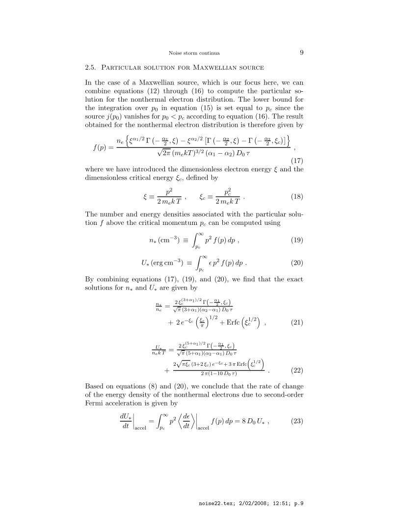
2.5. Particular solution for Maxwellian source

In the case of a Maxwellian source, which is our focus here, we cancombine equations (12) through (16) to compute the particular so-lution for the nonthermal electron distribution. The lower bound forthe integration over p0 in equation (15) is set equal to pc since thesource j(p0) vanishes for p0 < pc according to equation (16). The resultobtained for the nonthermal electron distribution is therefore given by

f(p) =ne

{

ξα1/2 Γ(

− α12 , ξ

)

− ξα2/2[

Γ(

− α22 , ξ

)

− Γ(

− α22 , ξc

)]

}

√2π (mekT )3/2 (α1 − α2)D0 τ

,

(17)where we have introduced the dimensionless electron energy ξ and thedimensionless critical energy ξc, defined by

ξ ≡ p2

2mek T, ξc ≡

p2c

2mek T. (18)

The number and energy densities associated with the particular solu-tion f above the critical momentum pc can be computed using

n∗ (cm−3) ≡∫ ∞

pc

p2 f(p) dp , (19)

U∗ (erg cm−3) ≡∫ ∞

pc

ǫ p2 f(p) dp . (20)

By combining equations (17), (19), and (20), we find that the exactsolutions for n∗ and U∗ are given by

n∗

ne=

2 ξ(3+α1)/2c Γ(−α1

2, ξc)√

π (3+α1)(α2−α1) D0 τ

+ 2 e−ξc

(

ξc

π

)1/2+ Erfc

(

ξ1/2c

)

, (21)

U∗

nek T =2 ξ

(5+α1)/2c Γ(−α1

2, ξc)√

π (5+α1)(α2−α1) D0 τ

+2√

πξc (3+2 ξc) e−ξc+ 3 π Erfc

(

ξ1/2c

)

2 π(1−10 D0 τ) . (22)

Based on equations (8) and (20), we conclude that the rate of changeof the energy density of the nonthermal electrons due to second-orderFermi acceleration is given by

dU∗dt

∣

∣

∣

∣

accel=

∫ ∞

pc

p2⟨

dǫ

dt

⟩∣

∣

∣

∣

accelf(p) dp = 8D0 U∗ , (23)

noise22.tex; 2/02/2008; 12:51; p.9

10 Subramanian & Becker

with U∗ computed using equation (22).

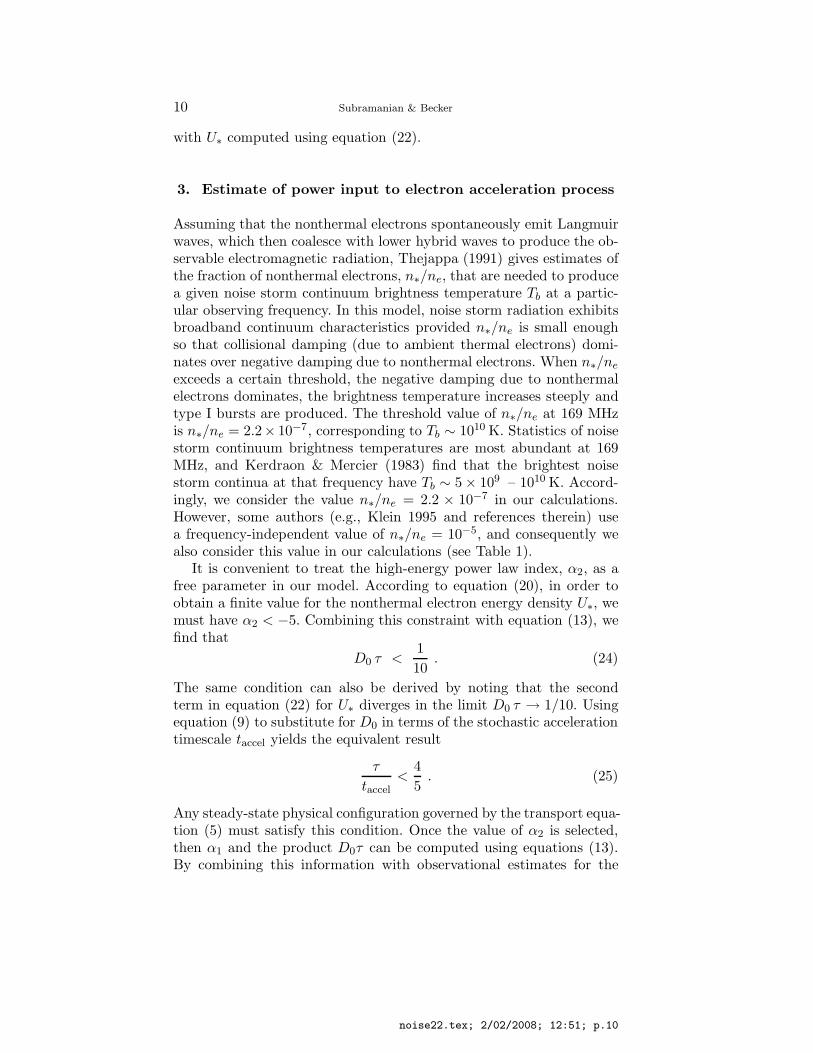
3. Estimate of power input to electron acceleration process

Assuming that the nonthermal electrons spontaneously emit Langmuirwaves, which then coalesce with lower hybrid waves to produce the ob-servable electromagnetic radiation, Thejappa (1991) gives estimates ofthe fraction of nonthermal electrons, n∗/ne, that are needed to producea given noise storm continuum brightness temperature Tb at a partic-ular observing frequency. In this model, noise storm radiation exhibitsbroadband continuum characteristics provided n∗/ne is small enoughso that collisional damping (due to ambient thermal electrons) domi-nates over negative damping due to nonthermal electrons. When n∗/ne

exceeds a certain threshold, the negative damping due to nonthermalelectrons dominates, the brightness temperature increases steeply andtype I bursts are produced. The threshold value of n∗/ne at 169 MHzis n∗/ne = 2.2× 10−7, corresponding to Tb ∼ 1010 K. Statistics of noisestorm continuum brightness temperatures are most abundant at 169MHz, and Kerdraon & Mercier (1983) find that the brightest noisestorm continua at that frequency have Tb ∼ 5 × 109 – 1010 K. Accord-ingly, we consider the value n∗/ne = 2.2 × 10−7 in our calculations.However, some authors (e.g., Klein 1995 and references therein) usea frequency-independent value of n∗/ne = 10−5, and consequently wealso consider this value in our calculations (see Table 1).

It is convenient to treat the high-energy power law index, α2, as afree parameter in our model. According to equation (20), in order toobtain a finite value for the nonthermal electron energy density U∗, wemust have α2 < −5. Combining this constraint with equation (13), wefind that

D0 τ <1

10. (24)

The same condition can also be derived by noting that the secondterm in equation (22) for U∗ diverges in the limit D0 τ → 1/10. Usingequation (9) to substitute for D0 in terms of the stochastic accelerationtimescale taccel yields the equivalent result

τ

taccel<

4

5. (25)

Any steady-state physical configuration governed by the transport equa-tion (5) must satisfy this condition. Once the value of α2 is selected,then α1 and the product D0τ can be computed using equations (13).By combining this information with observational estimates for the

noise22.tex; 2/02/2008; 12:51; p.10

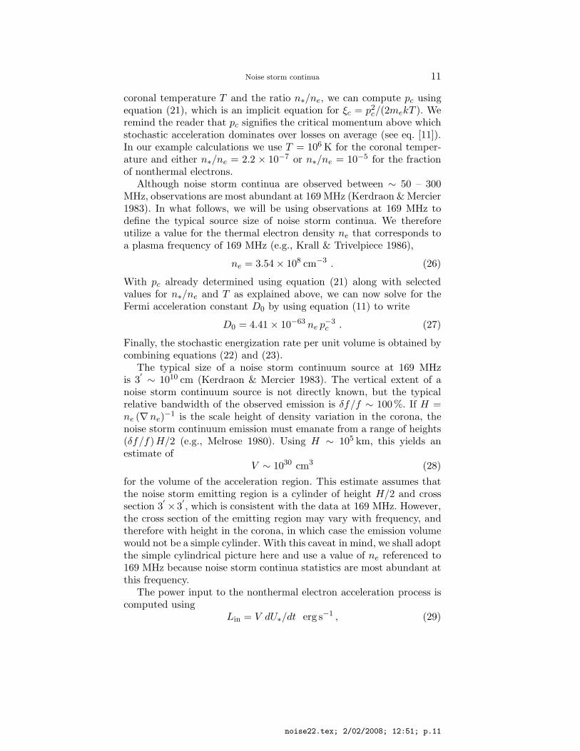
Noise storm continua 11

coronal temperature T and the ratio n∗/ne, we can compute pc usingequation (21), which is an implicit equation for ξc = p2

c/(2mekT ). Weremind the reader that pc signifies the critical momentum above whichstochastic acceleration dominates over losses on average (see eq. [11]).In our example calculations we use T = 106 K for the coronal temper-ature and either n∗/ne = 2.2 × 10−7 or n∗/ne = 10−5 for the fractionof nonthermal electrons.

Although noise storm continua are observed between ∼ 50 – 300MHz, observations are most abundant at 169 MHz (Kerdraon & Mercier1983). In what follows, we will be using observations at 169 MHz todefine the typical source size of noise storm continua. We thereforeutilize a value for the thermal electron density ne that corresponds toa plasma frequency of 169 MHz (e.g., Krall & Trivelpiece 1986),

ne = 3.54 × 108 cm−3 . (26)

With pc already determined using equation (21) along with selectedvalues for n∗/ne and T as explained above, we can now solve for theFermi acceleration constant D0 by using equation (11) to write

D0 = 4.41 × 10−63 ne p−3c . (27)

Finally, the stochastic energization rate per unit volume is obtained bycombining equations (22) and (23).

The typical size of a noise storm continuum source at 169 MHzis 3

′ ∼ 1010 cm (Kerdraon & Mercier 1983). The vertical extent of anoise storm continuum source is not directly known, but the typicalrelative bandwidth of the observed emission is δf/f ∼ 100%. If H =ne (∇ne)

−1 is the scale height of density variation in the corona, thenoise storm continuum emission must emanate from a range of heights(δf/f)H/2 (e.g., Melrose 1980). Using H ∼ 105 km, this yields anestimate of

V ∼ 1030 cm3 (28)

for the volume of the acceleration region. This estimate assumes thatthe noise storm emitting region is a cylinder of height H/2 and crosssection 3

′ ×3′, which is consistent with the data at 169 MHz. However,

the cross section of the emitting region may vary with frequency, andtherefore with height in the corona, in which case the emission volumewould not be a simple cylinder. With this caveat in mind, we shall adoptthe simple cylindrical picture here and use a value of ne referenced to169 MHz because noise storm continua statistics are most abundant atthis frequency.

The power input to the nonthermal electron acceleration process iscomputed using

Lin = V dU∗/dt erg s−1 , (29)

noise22.tex; 2/02/2008; 12:51; p.11

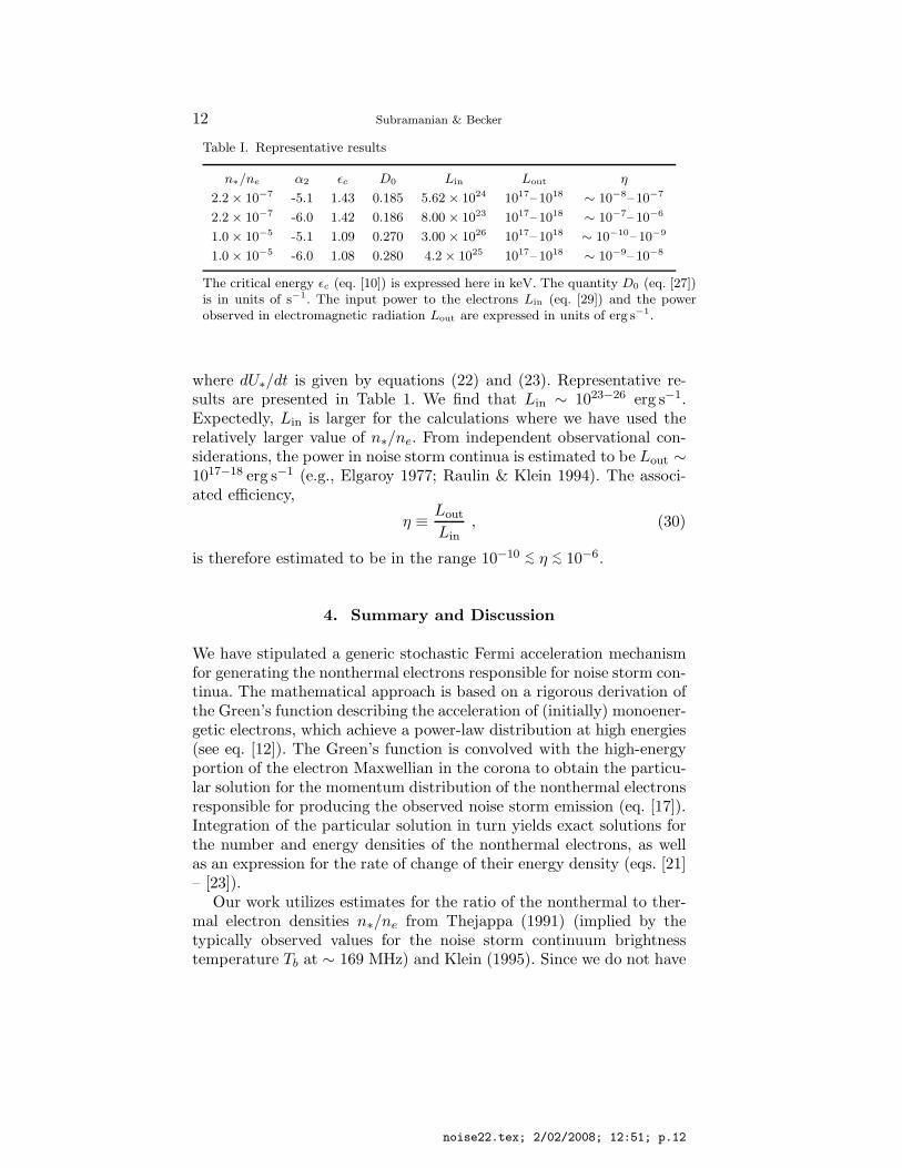
12 Subramanian & Becker

Table I. Representative results

n∗/ne α2 ǫc D0 Lin Lout η

2.2 × 10−7 -5.1 1.43 0.185 5.62 × 1024 1017– 1018 ∼ 10−8– 10−7

2.2 × 10−7 -6.0 1.42 0.186 8.00 × 1023 1017– 1018 ∼ 10−7– 10−6

1.0 × 10−5 -5.1 1.09 0.270 3.00 × 1026 1017– 1018 ∼ 10−10– 10−9

1.0 × 10−5 -6.0 1.08 0.280 4.2 × 1025 1017– 1018 ∼ 10−9– 10−8

The critical energy ǫc (eq. [10]) is expressed here in keV. The quantity D0 (eq. [27])is in units of s−1. The input power to the electrons Lin (eq. [29]) and the powerobserved in electromagnetic radiation Lout are expressed in units of erg s−1.

where dU∗/dt is given by equations (22) and (23). Representative re-sults are presented in Table 1. We find that Lin ∼ 1023−26 erg s−1.Expectedly, Lin is larger for the calculations where we have used therelatively larger value of n∗/ne. From independent observational con-siderations, the power in noise storm continua is estimated to be Lout ∼1017−18 erg s−1 (e.g., Elgaroy 1977; Raulin & Klein 1994). The associ-ated efficiency,

η ≡ Lout

Lin, (30)

is therefore estimated to be in the range 10−10 ∼< η ∼< 10−6.

4. Summary and Discussion

We have stipulated a generic stochastic Fermi acceleration mechanismfor generating the nonthermal electrons responsible for noise storm con-tinua. The mathematical approach is based on a rigorous derivation ofthe Green’s function describing the acceleration of (initially) monoener-getic electrons, which achieve a power-law distribution at high energies(see eq. [12]). The Green’s function is convolved with the high-energyportion of the electron Maxwellian in the corona to obtain the particu-lar solution for the momentum distribution of the nonthermal electronsresponsible for producing the observed noise storm emission (eq. [17]).Integration of the particular solution in turn yields exact solutions forthe number and energy densities of the nonthermal electrons, as wellas an expression for the rate of change of their energy density (eqs. [21]– [23]).

Our work utilizes estimates for the ratio of the nonthermal to ther-mal electron densities n∗/ne from Thejappa (1991) (implied by thetypically observed values for the noise storm continuum brightnesstemperature Tb at ∼ 169 MHz) and Klein (1995). Since we do not have

noise22.tex; 2/02/2008; 12:51; p.12

Noise storm continua 13

reliable observational estimates for the residence time τ of the electronsin the acceleration region, we instead parametrize the model using thehigh-energy power-law index α2 of the electron distribution function.We must restrict ourselves to values of α2 < −5 in order to obtain afinite value for the nonthermal electron energy density. By combiningan observational value for n∗/ne with a selected value for α2, we can useequation (21) to determine the critical momentum pc, which separatesthe thermal and nonthermal portions of the electron distribution. Theanalytical solution for the energy density of the nonthermal electrons isthen used to compute the energization rate due to second-order Fermiacceleration (see eqs. [22] and [23]).

Typical observational values for the total electron number densityne and the volume of the noise storm emitting region V were used toarrive at the results presented in Table 1. These results demonstratethat the power input to the electron acceleration process is around1023−26 erg s−1, which is 6–10 orders of magnitude larger than the powerthat is ultimately observed in the noise storm continuum radiation. Theefficiency of the process, starting from the acceleration of the nonther-mal electrons and culminating in the observable noise storm continuumradiation, is therefore in the range 10−10 ∼< η ∼< 10−6. Using data fromtype III decametric storms and impulsive 2–10 keV electron events at1 AU associated with type I noise storms, Lin (1985) estimates thatthe energy release rate for these electrons is around 1023 erg s−1 (cf. alsoJackson & Leblanc 1991). Klein (1995) estimates that the energy supplyto the energetic electrons is of the order of 1023−24 erg s−1. Prior to thecalculations presented here, these were the only (indirect, and ratherapproximate) estimates of the power input to nonthermal electronsrequired to drive noise storm radiation.

We believe that the general analysis of the energy budget presentedin this paper, based on a generic second-order Fermi energization mech-anism, will help to guide subsequent work on the detailed accelera-tion processes responsible for powering the noise storm continua. Ourresults also provide an important quantitative data point for discus-sions of electron acceleration in other high-temperature astrophysicalenvironments.

Acknowledgements

The authors are grateful to the anonymous referee who provided anumber of useful comments and suggestions which helped to improvethe manuscript. PS also acknowledges useful discussions with Prof.Monique Pick.

noise22.tex; 2/02/2008; 12:51; p.13

14 Subramanian & Becker

References

Becker, P. A.: 1992, Astrophys. J. 397, 88.Becker, P. A.: 2003, MNRAS 343, 215.Bentley, R. D., Klein, K.-L., van Driel-Gesztelyi, L., Demoulin, P., Trottet, G.,

Tassetto, P., Marty, G.: 2000, Solar Phys. 193, 227.Benz, A. O., Wentzel, D. G.: 1981, Astron. Astrophys. 94, 100.Brown, J. C.: 1972, Solar Phys. 25, 158 (Brown 1972a).Brown, J. C.: 1972, Solar Phys. 26, 441 (Brown 1972b).Brueckner, G. E.: 1983, Solar Phys. 85, 243.Chandran, B. D. G., Maron, J. L.: 2003, Astrophys. J. 603, 23.Crosby, N., Vilmer, N., Lund, N., Klein, K.-L., Sunyaev, R.: 1996, Solar Phys. 167,

333.Elgaroy, O.: 1977, Solar Noise Storms, Pergamon Press, Oxford.Jackson, B. V., Leblanc, Y.: 1991, Solar Phys. 136, 361.Kerdraon, A., Mercier, C.: 1983, Astron. Astrophys. 127, 132.Klein, K.-L.: 1995, in ‘Coronal Magnetic Energy Releases’, eds. A. O. Benz & A.

Kruger, Lecture Notes in Physics 444, Berlin: Springer, 55.Klein, K.-L.: 1998, in ‘Three-dimensional structure of solar active regions’, eds. C.

Alissandrakis & B. Schmeider, Astron. Soc. Pacific Conf. Series, 155, 182.Krall, N. A., Trivelpiece, A. W.: 1986, Principles of Plasma Physics, San Francisco

Press, San Francisco, CA.Krucker, S., Benz, A. O., Aschwanden, M. J., Bastian, T. S.: 1995, Solar Phys. 160,

151.Lin, R. P.: 1985, Solar Phys. 100, 537.Luo, Q. Y., Wei, F. S., Feng, X. S.: 2003, Astrophys. J. 584, 497.Malik, R. K., Mercier, C.: 1996, Solar Phys. 165, 347.Melrose, D. G.: 1980, Solar Phys. 67, 357.Miller, J. A., LaRosa, T. N., Moore, R. L.: 1996, Astrophys. J. 461, 445.Ptuskin, V. S.: 1988, Soviet Astron. Lett. 14, 255.Raulin, J.-P., Klein, K.-L.: 1994, Astron. Astrophys. 281, 536.Robinson, R. D.: 1978, Astrophys. J. 222, 696.Schlickeiser, R.: 2002, ‘Cosmic Ray Astrophysics’, Springer, Berlin.Smith, D. F.: 1977, Astrophys. J. 212, 891.Spicer, D. S., Benz, A. O., Huba, J. D.: 1981, Astron. Astrophys. 105, 221.Stewart, R. T., Brueckner, G. E., Dere, K. P.: 1986, Solar Phys. 106, 107.Subramanian, P., Becker, P. A., Kazanas, D.: 1999, Astrophys. J. 523, 203.Sundaram, G. A. Shanmuga, Subramanian, K. R.: 2004, Astrophys. J. 605, 948.Thejappa, G.: 1991, Solar Phys. 132, 173.Thejappa, G., Kundu, M. R.: 1991, Solar Phys. 132, 155.Wentzel, D. G.: 1985, Astrophys. J. 296, 278.Wentzel, D. G.: 1986, Solar Phys. 103, 141.Willson, R. F., Kile, J. N., Rothberg, B.: 1997, Solar Phys. 170, 299.

noise22.tex; 2/02/2008; 12:51; p.14