defects of micropolar continua in riemann-cartan manifolds
TRANSCRIPT
Defects of micropolar continua in Riemann-Cartan manifolds andits applications
Yongjo Lee
A thesis submitted in conformity with the requirements
for the degree of Doctor of Philosophy
Department of Mathematics
University College London
April 2021
Declaration
I, Yongjo Lee confirm, that the work presented in this thesis is my own. Where informationhas been derived from other sources, I confirm that this has been indicated in the thesis.
ii
Abstract
We derive equations of motion and its solutions in the form of solitons from deformationalenergy functionals of a coupled system of microscopic and macroscopic deformations. Thencriteria in constructing the chiral energy functional is specified to be included to obtain soliton-like solutions.
We show various deformational measures, used in deriving the soliton solutions, can bewritten when both curvature and torsion are allowed, especially by means of microrotationsand its derivatives. Classical compatibility conditions are re-interpreted leading to a universalprocess to derive a distinct set of compatibility conditions signifying a geometrical role of theEinstein tensor in Riemann-Cartan manifolds.
Then we consider position-dependent axial configurations of the microrotations to constructintrinsically conserved currents. We show that associated charges can be written as integersunder a finite energy requirement in connection with homotopic considerations. This furtherleads to a notion of topologically stable defects determined by invariant winding numbers for agiven solution classification.
Nematic liquid crystals are identified as a projective plane from a sphere hinted by thediscrete symmetry in its directors. Order parameters are carefully defined to be used bothin homotopic considerations and free energy expansion in the language of microcontinua. Mi-cropolar continua are shown to be the general case of nematic liquid crystals in projectivegeometry, and in formulations of the order parameter, which is also the generalisation of theHiggs isovectors.
Lastly we show that defect measures of pion fields description of the Skyrmions are relatedto the defect measures of the micropolar continua via correspondences between its underlyingsymmetries and compatibility conditions of vanishing curvature.
iii
Impact Statement
Descriptions of deformational propagations in coupled systems of microscopic and macro-scopic continua are shown to be the form of solitons. This further can be extended to a quantisedsoliton system which can be seen in the Euclidean Yang-Mills theory under the non-relativisticlimit.
A notion of zero curvature in the Einstein-Cartan theory is explicitly related to elasticityin the context of compatibility conditions. And homotopy groups are used to classify thesecompatibility conditions. This can be related to the theories in understanding the microscopicgravitation when one considers the elasticity in the curved space.
A construction of position-dependent axial microrotational fields as field configurations forconserved currents is discussed. Associated total charges of the conserved currents are shown tobe topologically and geometrically invariant integers. In constructing field configurations, chiralstructures on the given manifold is highly dependent on integers that embedded in axial fields.Hence, it can be useful to consider the origin of the chirality especially using projective geometry,for example in magnetic monopoles as seen as projected defects from higher dimensions.
Nematic liquid crystals are confirmed to be a special case of micropolar continua in termsof order parameters and its projective geometrical properties. Further, micropolar continua areidentified as projective space of the Skyrmions of the spin-isospin system, sharing an identicalform of the compatibility condition for vanishing curvature. A number of phases of superfluidliquid helium of 3He are known to exhibit similar symmetries of the spin-orbit system accompa-nied by the well-established order parameter formalism, which is much similar to that of nematicliquid crystals. Hence it is applicable to extend our generalisation of micropolar continua inthose phases of 3He.
iv
Acknowledgement
I would like to thank my supervisor Dr. Christian Böhmer for his kindness, patience, andinvitation into this wonderland of microcontinua. I would like to thank Dr. Franco Fiorini andDr. Santiago Hernández for their warm hospitality during my visit to Centro Atómico Bar-iloche, Departamento de Ingeniería en Telecomunicaciones and Instituto Balseiro, Argentina.Especially Dr. Franco Fiorini for stimulating discussions about "locally" invariant microrota-tions. I received enormous support from members of Department of Mathematics UCL duringmy Ph.D, and without them, this work would be impossible to finish.
v
Notations
a : 3-vector and 3-component quantitynv : normalised 2-component vortex fieldn3 : normalised 3-component fieldnN : normalised nematic liquid crystal fieldnh : normalised 3-component hedgehog fieldn4 : normalised 4-component fieldA : 3 × 3 matrix of M3(R)1 : 3 × 3 identity matrixa : arbitrary n-component tensorA : general n× n matrix of Mn(R,C)I : general n× n identity matrixz : complex conjugate of z ∈ CA∗ : complex conjugate of A ∈ Mn(C)A† : transpose of complex conjugate of A ∈ Mn(C)AT : transpose of A ∈ Mn(R,C)ui : displacement vector uuij : distortion tensor, grad u = ∂jui
ϵijk : Levi-Civita symbol, ϵ123 = 1 = −ϵ213Γ : Nye’s tensorF = ∇ψ = 1 + ∇u : deformation gradient tensorF = RU = polar(F )U : classical polar decompositionU = R
TF : first Cosserat deformation tensor
RT GradR : second Cosserat deformation tensor
(DivA)i = ∂jAij : divergence on the tensor A(CurlA)ij = ϵjkl∂kAil : curl on the tensor A(GradA)ijk = ∂kAij : gradient on the tensor A(Div (grad A))i = ∂j∂jAi : divergence on the tensor (grad A)ij = ∂jAi
(div A) = ∂iAi : divergence on the vector A(grad A)ij = ∂jAi : gradient on the vector A(curl A)i = ϵijk∂jAk : curl on the vector Asym M = (M +MT )/2 : symmetric part of matrix Mskew sym M = (M −MT )/2 : skew-symmetric part of Mdev M = M − tr(M)1/3 : deviatoric or trace-free part of MA : B = ⟨A,B⟩ = tr(ABT ) = tr(ATB) : Frobenius product of matrices A and B∥X∥2 = ⟨X,X⟩ = tr(XXT ) : Frobenius norm of X
vi
Contents
I Defects in microstructures 1
1 Microcontinuum 31.1 Introduction . . . . . . . . . . . . . . . . . . . . . . . . . . . . . . . . . . . . . . . 31.2 Deformational measures in classical and microcontinuum mechanics . . . . . . . 41.3 Deformational energy . . . . . . . . . . . . . . . . . . . . . . . . . . . . . . . . . 9
2 Dynamical Cosserat media 112.1 Energy functions . . . . . . . . . . . . . . . . . . . . . . . . . . . . . . . . . . . . 112.2 Equations of motion and solutions . . . . . . . . . . . . . . . . . . . . . . . . . . 132.3 Solution for the double sine-Gordon equation . . . . . . . . . . . . . . . . . . . . 172.4 Properties of solutions . . . . . . . . . . . . . . . . . . . . . . . . . . . . . . . . . 222.5 Galilean transformations and Lorentzian transformations . . . . . . . . . . . . . . 25
3 Chiral energy 293.1 Chiralities in continua . . . . . . . . . . . . . . . . . . . . . . . . . . . . . . . . . 293.2 Construction of chirality in deformational measures . . . . . . . . . . . . . . . . . 313.3 Constructing chiral energy functionals . . . . . . . . . . . . . . . . . . . . . . . . 333.4 Variations of a chiral equation . . . . . . . . . . . . . . . . . . . . . . . . . . . . . 343.5 Equations of motion and solutions . . . . . . . . . . . . . . . . . . . . . . . . . . 353.6 Constructing approximate solutions . . . . . . . . . . . . . . . . . . . . . . . . . . 37
II Defects in Riemann-Cartan manifolds 43
4 Background and motivation 454.1 Differential geometry and elasticity . . . . . . . . . . . . . . . . . . . . . . . . . . 454.2 Compatibility conditions . . . . . . . . . . . . . . . . . . . . . . . . . . . . . . . . 46
5 Deformational measures in Riemann-Cartan manifold 495.1 Frame fields and non-frame fields . . . . . . . . . . . . . . . . . . . . . . . . . . . 495.2 Torsion and curvature . . . . . . . . . . . . . . . . . . . . . . . . . . . . . . . . . 525.3 Einstein tensor in three-dimensional space . . . . . . . . . . . . . . . . . . . . . . 53
6 Compatibility conditions 556.1 Vallée’s classical result . . . . . . . . . . . . . . . . . . . . . . . . . . . . . . . . . 556.2 Nye’s tensor and its compatibility condition . . . . . . . . . . . . . . . . . . . . . 566.3 Eringen’s compatibility conditions . . . . . . . . . . . . . . . . . . . . . . . . . . 586.4 Geometrical compatibility conditions for the general case . . . . . . . . . . . . . 60
vii
7 Manifold structures and the compatibility conditions 637.1 Burgers vector and Frank’s vector . . . . . . . . . . . . . . . . . . . . . . . . . . 637.2 Homotopy for the compatibility conditions . . . . . . . . . . . . . . . . . . . . . . 65
III Defects in director fields 67
8 Theories of directors 698.1 Projective space and homotopy classification . . . . . . . . . . . . . . . . . . . . 69
8.1.1 Real projective space . . . . . . . . . . . . . . . . . . . . . . . . . . . . . . 708.1.2 Complex projective space . . . . . . . . . . . . . . . . . . . . . . . . . . . 728.1.3 Homotopy and projective space . . . . . . . . . . . . . . . . . . . . . . . . 73
8.2 Order parameter and homotopy . . . . . . . . . . . . . . . . . . . . . . . . . . . . 748.3 Nematic liquid crystals . . . . . . . . . . . . . . . . . . . . . . . . . . . . . . . . . 788.4 Free energy formalism and its expansion . . . . . . . . . . . . . . . . . . . . . . . 79
8.4.1 Order parameters in the energy expansion . . . . . . . . . . . . . . . . . . 798.4.2 Torsion terms in the energy expansion . . . . . . . . . . . . . . . . . . . . 828.4.3 Order parameter for the micropolar continua . . . . . . . . . . . . . . . . 85
9 Topological invariants and conserved currents 879.1 Simple soliton solutions in low dimensions . . . . . . . . . . . . . . . . . . . . . . 879.2 Conserved current, soliton and homotopy . . . . . . . . . . . . . . . . . . . . . . 91
9.2.1 Vortex field and winding number . . . . . . . . . . . . . . . . . . . . . . . 919.2.2 Conserved current in higher dimensions . . . . . . . . . . . . . . . . . . . 95
9.3 Topological sectors . . . . . . . . . . . . . . . . . . . . . . . . . . . . . . . . . . . 999.4 Polyakov’s hedgehog field . . . . . . . . . . . . . . . . . . . . . . . . . . . . . . . 103
10 Micropolar continuum and the Skyrme model 10510.1 Rotations of SO(3) and SU(2) . . . . . . . . . . . . . . . . . . . . . . . . . . . . 10510.2 Spinors . . . . . . . . . . . . . . . . . . . . . . . . . . . . . . . . . . . . . . . . . 108
10.2.1 Spin system . . . . . . . . . . . . . . . . . . . . . . . . . . . . . . . . . . . 10810.2.2 Fibration in the projective space . . . . . . . . . . . . . . . . . . . . . . . 10910.2.3 Hopf map . . . . . . . . . . . . . . . . . . . . . . . . . . . . . . . . . . . . 110
10.3 Skyrmions . . . . . . . . . . . . . . . . . . . . . . . . . . . . . . . . . . . . . . . . 11210.4 Micropolar in the projective space . . . . . . . . . . . . . . . . . . . . . . . . . . 115
11 Conclusions and outlooks 121
A Variations of energy functionals 123
B List of homotopy groups 127
viii
Part I
Defects in microstructures
1

Chapter 1
Microcontinuum
It all started from a question. What does microscopic deformation look like when a largebody undergoes elastic deformation? Then a following question arises. Can it be the samedescription that we know from the classical elasticity or something completely different? Thesame questions may have occurred to the brothers, François Cosserat (1852–1914) and EugéneCosserat (1866–1931), when they started to explore the theory of microscopic deformable body.In Part I, we would like to present solutions for deformational propagations in deformable media,based on the variational principle in attempting to understand deformations in coupled systemsof microscopic and macroscopic continua. Part I is mainly based on our published works [1, 2].
1.1 Introduction
Classical elasticity is based on considering materials whose idealised material points are struc-tureless. Any possible internal properties are neglected in the classical theory.
A microcontinuum, on the other hand, is a continuous collection of deformable materialpoints. The characteristic aspect of the theory with a microstructure is that we assume amicroelement to exhibit an inner structure attached to vectors called directors, which spaninternal three-dimensional space. Directors can rotate, compress and shear, independently ofmacroscopic deformations, to describe interior deformations of the microstructure.
The first ideas along those lines go back to the Cosserat brothers who pioneered such theories[3] back in 1909, fully in its geometrically nonlinear setting. In some ways, their work was aheadof their time and its significance had been overlooked for many decades. Starting from the 1950s,interests in this theory increased and many advances were made since then [4–7,7–13].
The most general elasticity theories with microstructure contain nine additional degrees offreedom which consist of three microrotations, one microvolume expansion, and five microsheardeformations. A comprehensive account of microcontinuum theories can be found in [9,14,15].A material structure of this generalised theory is called micromorphic and if we disregard themicroshear deformations from the micromorphic, the theory is called microstretch in whichthe directors can change its microvolume element and orientations under the microrotations.Some example of micromorphic continua include turbulent fluids, blood cell and some modelsof liquid crystals. Recent developments of nonlinear problems in generalised continua can befound in [16–20].
If we restrict these microdeformations to be rigid, so we further disregard the microshear,one deals with three degrees of freedom of the microrotations, in addition to the classicaltranslational deformation field. The resulting model is often referred to as Cosserat elasticityor micropolar theory. A few example of materials exhibiting the micropolar structure areferromagnetic fluids, and fluids of rigid microelements. Animal bone structures are particularly
3
good example of micropolar media, with pores in the bone are filled with micropolar materialswhich can undergo rigid microrotations.
We would like to consider the nature of microdeformation in micropolar models in whichthe rotation play a central role of the microscopic defects. If these deformations are timedependent, we wish to consider dynamic evolution of the microdeformations which may or maynot be coupled to the macroscopic deformational measures. To do so, we would like to startfrom total energy functions regarding microscopic and macroscopic deformations with a set ofappropriate classical and micropolar parameters. All other microscopic version of continuityequations, constitutive equations and balance laws can be found in the literatures introducedabove, especially in [3].
Once one can identify and collect the relevant energy functionals for the micropolar elasticity,equations of motion for the system can be found by the variational principle. Due to the highlynonlinear nature of the system, various attempts were made to simplify the process underrelatively weak restrictions and a simple ansatz. Spinor methods were used in [21] to simplifythe Euler-Lagrange equation and subsequent works appeared in [22, 23], with an intrinsicallytwo-dimensional model studied in [24]. In [25], polarity of ferromagnets gave rise to descriptionsof the defects in order parameters as solitary waves under external magnetic stimuli, followedby the study in the elastic crystals as a micropolar continuum in [26], again with descriptionsof soliton solutions for topological defects.
Variants of the geometrically nonlinear Cosserat model are also used to describe lattice rota-tions in metal plasticity in [27]. Further recent developments in the theory including nonlinearproblems in generalised continua were studied rigorously for instance in [16–20,28–31].
1.2 Deformational measures in classical and microcontinuummechanics
In a usual rectangular Cartesian coordinate system with the origin O, suppose we have a fixedregion of space R0 occupied by continuously distributed matter. After a subsequent time t,an original body B0 is moved or deformed to a new body B in the region R. One of criticalassumptions in continuum mechanics is that we are able to identify individual particle elementof the body so that we can track a point P in a body B0 at time t = 0 to a point p in B at anarbitrary time t.
Then the motion of B can be written as a function of the new position vector x dependenton the original position X and time t.
x = x(X, t) (1.2.1)
for all X ∈ R0 and x ∈ R. In practice, we can solve this for X to obtain
X = X(x, t). (1.2.2)
The configuration of B0 occupied by the position of particles at t = 0 is called the reference (ormaterial) configuration and we denote any quantity in the reference configuration by a capitalletter. The configuration of B with position of particles at x is called the spatial configurationand we denote quantities in this reference by a lower case. And we call the expression (1.2.2)as a spatial description in which we regard the spatial coordinate x as independent variablesand the expression (1.2.1) as the material description treating X as independent variables.
A displacement vector u describes macroscopic translations of a point particle at P with avector X to the point p with x and this can be written in the spatial description as
u(x, t) = x − X(x, t). (1.2.3)
4
In this way, we can write quantities such as velocity v, acceleration a, etc. in terms of eithermaterial or spatial description, defined by
v(X, t) = ∂u(X, t)∂t
, a = ∂v(X, t)∂t
. (1.2.4)
One of most important tensors describing deformations is a deformation gradient tensor Fdefined by
FkK = ∂xk
∂XK, (1.2.5)
which can be defined in a same way for the classical and microcontinuum theory. In the classicalcontinuum theory, this tensor can be decomposed using the polar decomposition as
F = RU = V R (1.2.6)
with a right stretch U and a left stretch tensor V satisfy, respectively,
U2 = F TF and V 2 = FF T . (1.2.7)
We assume that detF = 0 and it is obvious that F T is also second-order tensor and so isF−1, where
F−1Kk = ∂XK
∂xk. (1.2.8)
A displacement gradient tensor is defined by FiR − δiR, which is
FiR − δiR = ∂xi
∂XR− δiR = ∂ui
∂XR. (1.2.9)
A strain tensor is defined by the symmetric part of the displacement gradient tensor
uij = 12
(∂ui
∂xj+ ∂uj
∂xi
), uij = uji , (1.2.10)
where we made an approximation xi ≈ XR for small deformations.Next, we consider forces acting in an interior of continuous body. Suppose that a part of
a body B occupies a region R which has a surface S. Let P be a point on the surface S, n aunit vector directed along the outward normal to S at P and δS an area of an element of Swhich contains P . We assume that S and R possess any necessary smoothness and continuityproperties (e.g. it is assumed that the normal to S is uniquely defined at P ).
It is also assumed that on the surface element with area δS, the material outside R exertsforce on the material inside R.
δf = t(n)δS. (1.2.11)
Force δf is called surface force, and t(n) mean surface traction transmitted across the elementof area δS from the outside to the inside of R.
We can approximate that the surface traction t(n) becomes a quantity that is independentof the shape of the infinitesimal area as δS → 0 to write
t(n) = limδS→0
δf
δS. (1.2.12)
In a system of rectangular Cartesian coordinates, we can write t(n) with respect to the usualorthonormal base vectors ei by
ti = tijej , (1.2.13)
5

for i, j = 1, 2, 3. Using ei · ej = δij , this becomes
tij = ti · ej . (1.2.14)
Projection of the traction ti in the direction of ej will define a tensor tij called the stress tensor.For example, t11 is the component of t1 in the direction of e1. And t11 is positive if the materialon the x-positive side of the surface on which t1 acts is pulling the material on the x-negativeside. In particular, diagonal components t11, t22, t33 are called direct stress components andremaining components are called shearing stress components.
As an immediate application of the definition of the stress tensor, suppose the body in theregion R is in equilibrium so that resultant force and resultant couple about O on the continuumin the region is zero. These give a set of statements that∫
St(n) dS +
∫Rρg dV = 0 ,∫
Sx × t(n) dS +
∫Rρx × g dV = 0
(1.2.15)
where ρg is the body force (e.g. gravitational, electromagnetic forces) per unit volume.Using divergence theorem, (1.2.15) can be written in components∫
R
(∂tij∂xi
+ ρgj
)dV = 0 , (1.2.16a)∫
Rϵjpq
(∂
∂xr(xptrq) + ρxpgq
)dV = 0 . (1.2.16b)
The equation (1.2.16a) will give the equation of equilibrium,
∂tij∂xi
+ ρgj = 0 (1.2.17)
and (1.2.16b) will be reduced to ϵjpqtpq = 0, which characterises the symmetric property of thestress tensor,
tpq = tqp . (1.2.18)
A microcontinuum, on the other hand, is a continuous collections of deformable and stable(i.e. indestructible) material points [15]. We call these stable and deformable structures asparticles and a typical example of a particle in the microcontinuum is illustrated in Fig.1.1(right). A cesium chloride (CsCl) is often used to illustrate the inner structure of the microcon-tinuum [15] with Cs+ ion located at the centre of the cube and Cl− ions at eight corners of thecube. This model can be constructed from alternating layers of equally spaced cesium layers andchloride layers in bulk. The cubane of chemical formula C8H8 with its genuine individual cubicmolecular structure provides good model of micropolar medium with eight hydrogen moleculesare attached in the conners of the cubic. In cesium chloride model, we can assign a position ofCs+ a vector X at P in the material configuration but at this time, we need an additional set ofvectors for Cl− to describe the inner structure of the cubic crystalline solid and its deformations.
In other words, the particles are assumed as point particles with infinitesimal size in theclassical theory. But since they are deformable by definition in the microcontinuum theory, itis clear that we need an extra set of degrees of freedom to describe the theory of these particle’sdeformability, in addition to the vectors assigned to P in the classical theory as being treatedas a point particle. This means, in addition to the classical translational deformation field, thebody as a collection of point particle P can be deformable in a classical (macroscopic scale) wayand the inner structure of the particle can only experience microdeformations.
6
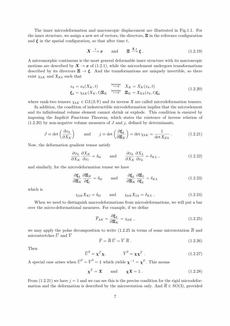
The inner microdeformation and macroscopic displacement are illustrated in Fig.1.1. Forthe inner structure, we assign a new set of vectors, the directors, Ξ in the reference configurationand ξ in the spatial configuration, so that after time t,
Xt−→ x and Ξ X,t−→ ξ . (1.2.19)
A micromorphic continuum is the most general deformable inner structure with its macroscopicmotions are described by X → x of (1.2.1), while the microelement undergoes transformationsdescribed by its directors Ξ → ξ. And the transformations are uniquely invertible, so thereexist χkK and XKk such that
xk = xk(XK , t) inverse−→ XK = XK(xk, t)ξk = χkK(XK , t)ΞK
inverse−→ ΞK = XKk(xk, t)ξk
(1.2.20)
where rank-two tensors χkK ∈ GL(3; R) and its inverse X are called microdeformation tensors.In addition, the condition of indestructible microdeformation implies that the microelement
and its infinitesimal volume element cannot shrink or explode. This condition is ensured byimposing the Implicit Functions Theorem, which states the existence of inverse relation of(1.2.20) by non-negative volume measures of J and j, defined by determinants,
J ≡ det(∂xk
∂XK
)and j ≡ det
(∂ξk
∂ΞK
)= detχkK = 1
detXKk. (1.2.21)
Now, the deformation gradient tensor satisfy
∂xk
∂XK
∂XK
∂xl= δkl and ∂xk
∂XK
∂XL
∂xk= δKL , (1.2.22)
and similarly, for the microdeformation tensor we have
∂ξk
∂ΞK
∂ΞK
∂ξl
= δkl and ∂ξk
∂ΞK
∂ΞL
∂ξk
= δKL (1.2.23)
which isχkKXKl = δkl and χkKXLk = δKL . (1.2.24)
When we need to distinguish macrodeformations from microdeformations, we will put a barover the micro-deformational measures. For example, if we define
F kK = ∂ξk
∂ΞK= χkK , (1.2.25)
we may apply the polar decomposition to write (1.2.25 in terms of some microrotation R andmicrostretches U and V
F = R U = V R . (1.2.26)
ThenU
2 = χT χ, V2 = χχT . (1.2.27)
A special case arises when U2 = V
2 = 1 which yields χ−1 = χT . This means
χT = X and χX = 1 . (1.2.28)
From (1.2.21) we have j = 1 and we can see this is the precise condition for the rigid microdefor-mation and the deformation is described by the microrotation only. And R ∈ SO(3), provided
7
Figure 1.1: On the left, the transformation of the inner structure of the microelement with centroidspositioned at P and p in the reference configuration and the spatial configuration, respectively, is illus-trated. This shows how the directors Ξ in the original body B0 undergoes microdeformation under χkK
transform to ξ, while the original body B0 experiences displacement to become a deformed configurationbody B in three-dimensional space under the macroscopic displacement u. The typical particle modelledby cubane as a micropolar continuum is shown in its microscopic cubic molecular structure in the bulkbody on the right.
we can rescale the magnitude of the directors Ξ, ξ to unity to retain the rigidity of the innerstructure.
A microstretch continuum is characterised by the property
XKk = 1j2χkK . (1.2.29)
As illustrated in Fig.1.1, the microrotations R are responsible for the inner rotations of thedirectors such that
ξk = RkKΞK and ΞK = RKkξk . (1.2.30)The finite microrotation of an angle ϕ about a normalised axis n is represented by Rkl,
Rkl = cosϕ δkl − sinϕ ϵklmnm + (1 − cosϕ)nknl (1.2.31)
whereϕ = (ϕkϕk)1/2, nk = ϕk
ϕ, Rkl = RkLδLl (1.2.32)
For small rotations, the expression (1.2.31) becomes
Rkl ≈ δkl − ϵklmϕm . (1.2.33)
i.e. the rotation tensor can be represented by a vector ϕk, and this limit becomes apparentwhen one represents the rotation by an exponential of an antisymmetric matrix as in (8.4.13).In classical continuum mechanics, the macrorotation tensor due to a change of line elements is
RkK = ∂xk
∂XLC
−1/2LK . (1.2.34)
8
This follows from the polar decomposition (1.2.6), where CLK is the classical deformation tensorknown as the right Cauchy-Green tensor, defined by
CLK = ∂xk
∂XL
∂xk
∂XK, C = F TF. (1.2.35)
In the linear theory, the macrorotation (1.2.34) reduces to an infinitesimal rotation tensor inclassical continuum mechanics,
Rkm ≡ Rkm − δkm = 12
(∂uk
∂xm− ∂um
∂xk
), (1.2.36)
where uk is the displacement vector. For small angle consideration, from (1.2.33) and (1.2.36),we can identify the difference between macrorotation R and microrotation R.
We introduce some useful deformational measures as follows.
CKL ≡ ∂xk
∂XK
∂ΞL
∂ξk= ∂xk
∂XKXLk = ∂xk
∂XKχkL
CKL ≡ ∂ξk
∂ΞK
∂ξk
∂ΞL= χkKχkL = CLK
ΓKLM ≡ ∂ΞK
∂ξk
∂χkL
∂XM= XKk
∂χkL
∂XM
(1.2.37)
where CKL is called the deformation tensor, CKL the microdeformation tensor, and ΓKLM thewryness tensor. In case of micropolar continua, the deformation tensor CKL is known as thefirst Cosserat deformation tensor and the wryness tensor reduces to
ΓKL = 12ϵKMN
∂χkM
∂XLχkN , (1.2.38)
from which we recognise χkN ∈ SO(3).
1.3 Deformational energyWe would like to look at formulation of an energy function Velastic(F,R) in a coupled form of thedisplacement gradient tensor F and the microrotation R, and an energy function Vcurvature(R)due to the microrotation entirely and its implications briefly. More comprehensive treatmentsin deriving general energy functionals can be found in [21,23].
In constructing energy functions, we must note that the energy function must be a functionof the strain tensor (classical or microcontinuum), as emphasised in [32]. In addition, we wouldlike to have each term in the energy functionals remains invariant under the rotation, if therigidity in the microelement is imposed. These conditions in formulating the energy functionalssuggest that we need a set of independent scalars of second-order tensors to form the energyfunctional. For this purpose, we introduce the Cartan-Lie decomposition for any 3 × 3 matrixM ,
M = dev sym M + skew M + 13trM · 1 , (1.3.1)
where dev sym M is the traceless symmetric part of M and skew M is the skew-symmetric partof M .
The most general form of the energy function, in the classical theory, Vclassical satisfyingabove mentioned conditions is
Vclassical = µ∥uij∥2 + λ
2 ∥uii∥2 , (1.3.2)
9
where µ and λ are called Lamé coefficients. The first term on the right-hand side representsthe energy associated to the pure shear and the second term represents the energy associatedto the volumetric expansion (or compression). These can be seen if one calculate and comparea undeformed volume element dV and a deformed volume element dV ′.
The energy function (1.3.2) indeed leads to the classical Hooke’s law and the force f isdefined by
fi = ∂tij∂xj
. (1.3.3)
By Newton’s third law, interaction between two forces fi and fj (i = j) is cancelled internally.Hence the total force per unit volume f is a sum of the individual fi for a given internal surfaceelement of the body, so that we can write∑
i
∫Rfi dV =
∫R
f dV . (1.3.4)
The resultant integral on the right-hand side of (1.3.4) represents the sum of all forces actingon all surface element for a given body volume. In other words, the sum of integral over a givenvolume element is transformed into the integral over the surface elements, and all the internalstresses can be transformed into integral over the surface. This agrees with the definition offorce given in (1.3.3) and (1.2.11) in terms of the stress tensor, hence we can write∫
Rfi dV =
∫R∂jtij dV =
∫Stij dSj . (1.3.5)
We can generalise this idea in formulating the elastic energy functionals for the microcon-tinuum theory. Using the decomposition (1.3.1), we can write
Velastic(F,R) = µ∥∥∥sym(RT
F − 1)∥∥∥2
+ λ
2[tr(sym(RT
F − 1))]2
(1.3.6)
where the term RTF is the first Cosserat deformation tensor in the coupled system of microro-
tation R and the classical displacement gradient tensor F . Analogous to (1.3.2), the first termon the right-hand side of (1.3.6) represents energy for the pure shear and the quantity RT
F − 1is symmetrised in accordance with the symmetric classical strain tensor uij , which can be seendirectly from (1.2.9) under the limit R → 1. The second term of (1.3.6) represents energyassociated to the volumetric expansion. Hence, we can see that the elastic energy functional(1.3.6) is a natural generalisation of the classical expression (1.3.2).
10
Chapter 2
Dynamical Cosserat media
In Section 2.1, we present the full treatment for solutions of elastic and rotational propagationsof deformations in the complete dynamical Cosserat problem. This involves a total energyfunctional given by
V = Velastic(F,R) + Vcurvature(R) + Vinteraction(F,R) + Vcoupling(F,R) .
We will obtain equations of motion, from variations ofδVtotalδF
and δVtotal
δR(2.0.1)
where Vtotal is energy function including kinetic terms.Primary mathematical interests in finding the equations of motion using the variational
calculus come from the fact that many terms in the energy functionals contain quantities suchas
RT CurlR , R
T polar(F ) , RTF
throughout the calculations. Since, in general, the elements in SO(3) do not commute, thevariations require careful treatment in the calculations. There are two approaches we can takein varying those quantities. One way is to put a Lagrangian multiplier λ in a Lagrangian Lin a form of λ(RTR − 1) to obtain the Euler-Lagrangian equation, and another is to use theexponential representation of the rotational matrix R = eA under certain condition such as thesmall rotational angle assumption.
In Section 2.2, after stating each energy functional in terms of F and R, we use the variationof the total energy functional including kinetic energy terms. We collect terms from variationalfield expressions with respect to F and R, to obtain a complete coupled system of equationsof motion. It turns out that if we impose certain set of restrictions (e.g. small displacements),newly generated nonlinear coupling terms in the complete description are indeed responsible forthe contribution in additional terms of the sine-Gordon type equation.
This observation reduces the problem to solving the double sine-Gordon equation [33] of afunction of ϕ = ϕ(z, t). In the final part, we illustrate effects of rotational and displacementpropagations in a simple model of microcontinua with additional features of a kink-antikinkform of solutions, and profiles of a wave number k and a wave velocity v.
2.1 Energy functionsIf we assign a set of time-dependent functions to a microrotational measure R and a macroscopicdisplacement gradient F , the field equations will be descriptions of propagating defects in acertain direction.
11

We introduce each energy functional for the full treatment of the geometrically nonlinearCosserat problem in three-dimensional space. We will include kinetic energy terms to appro-priate energy functionals before deriving the equations of motion. First, the energy functionalfor elastic deformations is
Velastic(F,R) = µ∥∥∥sym(RT
F − 1)∥∥∥2
+ λ
2[tr(sym(RT
F − 1))]2
(2.1.1)
where λ and µ are the standard Lamé parameters. The microrotations are governed byVcurvature(R),
Vcurvature(R) = κ1∥∥∥dev sym(RT CurlR)
∥∥∥2+ κ2
∥∥∥skew(RT CurlR)∥∥∥2
+ κ3[tr(RT CurlR)
]2 (2.1.2)
where κi are the elastic constants for the microrotations. The operation of Curl on any 3 × 3matrix M is defined by
CurlM =
∂yM13 − ∂zM12 ∂zM11 − ∂xM13 ∂xM12 − ∂yM11∂yM23 − ∂zM22 ∂zM21 − ∂xM23 ∂xM22 − ∂yM21∂yM33 − ∂zM32 ∂zM31 − ∂xM33 ∂xM32 − ∂yM31
(2.1.3)
or in components, this is(CurlM)ij = ϵjkl∂kMil . (2.1.4)
Formulation of this energy functional follows immediately from the decomposition of (1.3.1)with the required conditions mentioned before. The quantity
RT CurlR (2.1.5)
is called a dislocation density tensor and it originates back in Nye’s pioneering work [34]. Afairly straightforward explanation of this quantity can be found in [35], in developing a totaldisplacement known as Burgers vector, caused by continuous distribution of dislocations (hencethe name). We will find that this rank-two tensor (2.1.5) will be one of our central ingredientsin understanding both in microscopic and macroscopic deformations especially when we regardthe notion of torsion, accompanied by more formal definition and its use in Part II.
Interaction between elastic displacements and microrotations is described by irreducibleparts of the elastic deformations and microrotations, such as RT
F−1 and RT CurlR respectively,to form a energy functional Vinteraction(F,R), defined by
Vinteraction(F,R) = χ1tr(RT CurlR)tr(RTF )
+ χ3⟨dev sym(RT CurlR), dev sym(RTF − 1)⟩.
(2.1.6)
where χ1 and χ3 are coupling constants, while the vanishing χ2 term can be seen from theabsence of skew(RT
F − 1) term in (2.1.1). We denote the Frobenius product of matrices A andB by
⟨A,B⟩ = A : B = tr(ABT ) = tr(ATB) .Lastly, we will consider the Cosserat coupling term which is given by
Vcoupling(F,R) = µc
∥∥∥RT polar(F ) − 1∥∥∥2
(2.1.7)
where µc is the Cosserat couple modulus, and polar(F ) is the polar part in the classical de-composition of F = RU . This energy function explicitly distinguishes the microrotation R and
12
the macrorotation defined by polar(F ), but express non-trivial coupled energy between them.This can be easily seen from the fact that Vcoupling(F,R) vanishes when R → polar(F ). Couplemodulus in the classical elastic theory can be found in [6, 36], and various limiting cases of theCosserat couple modulus are studied in [37,38].
Variations of the energy functionals, in the following expression, are quite technically in-volved.
δV (F,R) = δVcoupling(F,R) + δVinteraction(F,R) + δVelastic(F,R) + δVcurvature(R) . (2.1.8)
All detailed results are stated explicitly in Appendix A, but the principle idea is to vary termby term according to the basic variational calculus such as
δV (F,R) = ∂V
∂F: δF + ∂V
∂R: δR
with the help of chain rules in varying the matrices summarised in Appendix A.Now, we gather all the variational terms (A.0.5), (A.0.13), (A.0.15) and (A.0.19), we will
obtain the complete variational functional of the theory for the dynamical case as follows.
δVelastic(F,R) =[µ(RF TR+ F ) − (2µ+ 3λ)R+ λtr(RT
F )R]
: δF
+[µFR
TF − (2µ+ 3λ)F + λtr(RT
F )F]
: δR+ ρu δu (2.1.9a)
δVcurvature(R) =[(κ1 − κ2)
((CurlR)RT (Curl (R)) + Curl
[R(CurlR)TR
])+ (κ1 + κ2)Curl
[CurlR
]−(κ13 − κ3
)(4tr(RT CurlR)Curl (R) − 2R
(grad
(tr[RT CurlR]
))⋆+ 2ρrotR
]: δR
(2.1.9b)
δVinteraction(F,R) =(χ1 − χ3
3)(
2tr(RTF )Curl (R) + tr(RT CurlR)F −R
[grad
(tr[RT
F ])]⋆)
+ χ32(Curl (F ) + (Curl (R))RT
F + FRT (Curl (R)) + Curl (RF TR)
): δR
(2.1.9c)
+χ1tr(RT CurlR)R+ χ3
2(Curl (R) +R(Curl (R))TR
)− χ3
3 tr(RT Curl (R))R
: δF
δVcoupling(F,R) = −2µcR : δR− 2µc
det(Y )[RY (RTR−R
TR)Y
]: δF (2.1.9d)
where dots imply the time derivatives for the variation in the kinetic terms ρu δu = ρ∂ttψ δψ.We defined Y = tr(U)1 − U , and the kinetic term for Vcurvature by
Vcurvature,kinetic = ρrot∥R∥2 = ρrottr(R RT ) .
The next step will be collecting various expressions with respect to F and R to construct thefield equations.
2.2 Equations of motion and solutionsIn the recent paper [39], the dynamical Cosserat model was investigated by analysing the ge-ometrically nonlinear and coupled nature of the system, in which linearised energy functionalsare considered to simplify the problem. It allowed reduction of the coupled system of partialdifferential equations to a sine-Gordon equation, which in turn yielded soliton solutions both in
13
microrotational and displacement deformations under the assumption that displacements aresmall while microrotations can be arbitrarily large.
By the nature of micropolar continua, the microrotation can be represented by an arbitraryrotational angle ϕ = ϕ(x, y, z, t) about an arbitrary axis n = n(x, y, z, t) in three spatial dimen-sions. In other words, every individual point in the micropolar continua can have independentrigid rotational degrees of freedom. Moreover, since we are dealing with the dynamic problem,an elastic wave (if there is any) of microrotation ϕ and macrodeformation ψ can propagate in-dependently with different velocities which may propagate in the form of either longitudinal ortransverse through the given media in each case, hence four different combinations are possible.This means, if we consider a general case, the equations of motion would be highly nonlinearby nature, and it might not be possible to solve them analytically. Therefore, we would like tomake following assumptions.
1. We assume that points in our microcontinuum can only experience rotations about a fixedaxis, say the z-axis, which allows us to write
R =
cosϕ − sinϕ 0sinϕ cosϕ 0
0 0 1
. (2.2.1)
In this case, the variation of microrotation is simply
δR =
− sinϕ δϕ − cosϕ δϕ 0cosϕ δϕ − sinϕ δϕ 0
0 0 0
. (2.2.2)
2. We will look for solutions of ϕ and ψ, or coupled system, in which both microrotationaland macro-displacement waves are longitudinal about the same axis, the z-axis in thiscase, so that we can write forms of wave equations by
Microrotation: ϕ = ϕ(z, t)Macro displacement: ψ = ψ(z, t) .
(2.2.3)
Hence the displacement vector, in F = 1 + ∇u, is just
u =
00
ψ(z, t)
and ∇u =
0 0 00 0 00 0 ∂zψ(z, t)
. (2.2.4)
Under these assumptions, we might expect that the dynamic problem will be simplified sig-nificantly while the central properties of Cosserat problem are retained, but even with thesesimplified situation, the equations to be solved can be quite challenging.
We are ready to collect relevant terms with respect to F and R separately. Unlike the caseof δR, in which the variational kinetic term is readily written with respect to R, the variationalkinetic term from the interaction energy functional is written with respect to δu. But thevariation with respect to F can be restated as the variation with respect to u, hence withrespect to ψ as we will see shortly.
14
Collecting terms for δF from (2.1.9) gives
A11 A12 0−A12 A11 0
0 0 A33
=[µ(RF TR+ F
)− (2µ+ 3λ)R+ λtr(RT
F )R]
+[χ1tr
(R
T CurlR)R+ χ3
2(CurlR+R(CurlR)TR
)− χ3
3 tr(R
T CurlR)R
]+ 2µc
det Y[RY
(R
TR−RTR
)Y], (2.2.5)
where
A11 = 13 cosϕ
[6(λ+ µ)(−1 + cosϕ) + (6χ1 + χ3)∂zϕ+ 3λ∂zψ
]A12 = −1
3 sinϕ[−6λ− 6µ+ 6λ cosϕ+ 6µ cosϕ− 6µc + (6χ1 + χ3)∂zϕ+ 3λ∂zψ
]A33 = 2λ(−1 + cosϕ) +
(2χ1 − 2χ3
3
)∂zϕ+ (λ+ 2µ)∂zψ .
(2.2.6)
Now, the terms which appear in the variation with respect to F can be transformed into thevariation with respect to ∇u, for any matrix A, as shown below.
A : δF = AijδFij −→ −∂jAijδui = −(∂1A31 + ∂2A32 + ∂3A33)δψ , (2.2.7)
up to a boundary term. In this case, the contribution comes only from A33 ,and we are left with
[2λ sinϕ ∂zϕ−
(2χ1 − 2χ3
3
)∂zzϕ− (λ+ 2µ)∂zzψ
]δψ . (2.2.8)
We now include the kinetic variational term ρu δu = ρ∂ttψ δψ to obtain the equation ofmotion for F ,
− λ (∂zzψ − 2∂zϕ sinϕ) − 2µ∂zzψ + ρ∂ttψ + 23(χ3 − 3χ1)∂zzϕ = 0 . (2.2.9)
In the same way, we collect terms for δR to obtain
B11 B12 0−B12 B11 0
0 0 B33
= 2ρrotR+ µFRTF − (2µ+ 3λ)F + λtr(RT
F )F − 2µcR
+ (κ1 − κ2)[(CurlR)RT (CurlR) + Curl
(R(CurlR)TR
)]+ (κ1 + κ2)
[Curl (CurlR)
]−(κ13 − κ3
) [4tr(RT CurlR)CurlR− 2R
(grad
[tr(RT CurlR)
])⋆]+(χ1 − χ3
3
)(2tr(RT
F )CurlR+ tr(RT CurlR)F −R[grad(tr(FRT ))
]⋆)+ χ3
2(CurlF + (CurlR)RT
F + FRT (CurlR) + Curl (RF TR)
)(2.2.10)
15
where
B11 = − 2(λ+ µ+ µc) + 6χ1 cos2 ϕ ∂zϕ+ λ∂zψ
+ 13 cosϕ
[3(2λ+ µ) − 6ρrot(∂tϕ)2 + (κ1 − 3κ2 + 24κ3)(∂zϕ)2 + 2(3χ1 − χ3)∂zϕ(1 + ∂zψ)
]+ 1
3 sinϕ[−6ρrot∂ttϕ+ 2(κ1 + 6κ3)∂zzϕ+ (3χ1 − χ3)∂zzψ
]B12 =1
3 sinϕ[3µ+ 6ρrot(∂tϕ)2 − (κ1 − 3κ2 + 24κ3)(∂zϕ)2 − 2(3χ1 − χ3)∂zϕ(1 + ∂zψ)
]+ cosϕ
[−6χ1 sinϕ ∂zϕ+ 1
3 (−6ρrot∂ttϕ+ 2(κ1 + 6κ3)∂zzϕ+ (3χ1 − χ3)∂zzψ)]
B33 = − 2µc + 2λ cosϕ(1 + ∂zψ) + 13(1 + ∂zψ)
[(6χ1 − 2χ3)∂zϕ+ 3(−2λ− µ+ (λ+ µ)∂zψ)
].
(2.2.11)
Applying B : δR gives
B : δR = tr[BT δR
]= −(2B11 sinϕ+ 2B12 cosϕ)δϕ , (2.2.12)
which is [4(λ+ µ+ µc) sinϕ− 2(λ+ µ) sin 2ϕ− 2λ sinϕ ∂zψ + 4ρrot∂ttϕ
− 4(κ13 + 2κ3
)∂zzϕ− 2
(χ1 − χ3
3
)∂zzψ
]δϕ .
(2.2.13)
Therefore, from (2.2.9) and (2.2.13), we obtain two equations of motion by varying the totalenergy functional with respect to F and R, respectively, as follows
− (λ+ µ+ µc) sinϕ+ 12(λ+ µ) sin 2ϕ+ 1
2λ sinϕ∂zψ − ρrot∂ttϕ
+(κ13 + 2κ3
)∂zzϕ+
(χ12 − χ3
6
)∂zzψ = 0 , (2.2.14a)
− λ (∂zzψ − 2∂zϕ sinϕ) − 2µ∂zzψ + ρ∂ttψ + 23(χ3 − 3χ1)∂zzϕ = 0 . (2.2.14b)
These can be written in components form by(∂ttϕ∂ttψ
)= M
(∂zzϕ∂zzψ
)+(
0 λ sin ϕ2ρrot
−2λ sin ϕρ 0
)(∂zϕ∂zψ
)− (λ+ µ+ µc)
ρrot
(sinϕ
0
)+ λ+ µ
2ρrot
(sin 2ϕ
0
)(2.2.15)
whereM =
((κ1 + 6κ3)/3ρrot (3χ1 − χ3)/6ρrot2(3χ1 − χ3)/3ρ (λ+ 2µ)/ρ
). (2.2.16)
From this, we can see immediately that the off-diagonal entries of M are responsible for thecoupled system, and due to the remaining nonlinear terms, it is difficult to diagonalise the wholesystem to uncouple the variables. Also, we note that we will recover the result obtained in [39]if we assume the linearised energy functionals which lead to the approximations such as λϕ ≪ 1and µϕ ≪ 1, while the matrix elements M remain unchanged.
A similar problem was investigated in [26], and its revised results were stated in [15], inwhich case the longitudinal wave is expressed as the displacement vector u(x, t) along the x-axis with the rotational deformation ϕ(x, t) about x-axis. The equations of motion are described
16
as a system of coupled expressions,(∂ttϕ∂ttu
)= N
(∂xxϕ∂xxu
)+(
0 2λ′ sin ϕρ0J
−2(λ′+2µ′+κ′) sin ϕρ0
0
)(∂xϕ∂xu
)+ 2λ′
ρ0J
(sinϕ
0
)+ 2λ′ + µ′
ρ0J
(sin 2ϕ
0
)(2.2.17)
where α, λ′, µ′, κ′ are isotropic material moduli used in [15], and
N =(
αρ0J 00 λ′+2µ′+κ′
ρ0
). (2.2.18)
Since the matrix N is diagonal, we do not have second order coupling terms in the equationsof motion. Unlike our current case, the system (2.2.17) is readily solvable under the smalldisplacement limit, using the conventional method for the one-dimensional d’Alembert’s solutionsubject to appropriate boundary conditions.
2.3 Solution for the double sine-Gordon equation
What we obtained so far is a system of nonlinear coupled partial differential equations (2.2.14)and a non-diagonal matrix representation of M in (2.2.16). We note that we cannot make anyassumptions for the parameters in M unless any specific physical system is assumed to simplifythe problem significantly.
We will generalise the previously considered deformations in [39] of limited case to includethe fully nonlinear model with arbitrarily large rotations and displacements. This discussionwill give us further insights into the nature of the nonlinear geometry of Cosserat micropolarelasticity.
Now, before we solve the equations, we make an additional assumption that the elastic androtational waves propagate with the same constant wave speed v, and ψ = g(z − vt), so that ψsatisfies
∂ttψ = v2∂zzψ . (2.3.1)
First, we denote the diagonal entries of M by v2rot = M11 and v2
elas = M22. Then (2.2.14b)becomes
g′′(z − vt) = ∂zzψ = M21v2 − v2
elas∂zzϕ− 2λ
ρ(v2 − v2elas)
sinϕ ∂zϕ . (2.3.2)
Integrating with respect to z once gives
g′(z − vt) = ∂zψ = M21v2 − v2
elas∂zϕ+ 2λ
ρ(v2 − v2elas)
cosϕ (2.3.3)
in which we set the constant of integration to zero by imposing following boundary conditionsfor ψ = g(z − vt),
ψ(±∞, t) = 0 and ∂zψ(±∞, t) = 0 . (2.3.4)
The first asymptotic condition for ψ(z, t) is reasonable in a sense that the elastic macrodeforma-tion will not affect the point located far away from the place where the deformation currentlyoccurs, and the material point should return to its original configuration as we approach spatialinfinity z → ±∞. The second condition follows from the finite energy requirement when oneintegrate over the region for the continuum.
17
Substituting (2.3.2) and (2.3.3) into the remaining equation of motion (2.2.14a) gives
∂ttϕ−[v2
rot + M12M21v2 − v2
elas
]∂zzϕ− λ
2(v2 − v2elas)
[M21ρrot
− 4M12ρ
]sinϕ ∂zϕ
+ (λ+ µ+ µc)ρrot
sinϕ−[
λ2
2ρrotρ(v2 − v2elas)
+ λ+ µ
2ρrot
]sin 2ϕ = 0 .
(2.3.5)
Moreover, if we rescale z by
z =(v2
rot + M12M21v2 − v2
elas
)1/2
z (2.3.6)
then (2.3.5) reduces to, the double sine-Gordon equation
∂ttϕ− ∂zzϕ+m2 sinϕ+ b
2 sin 2ϕ = 0 , (2.3.7)
wherem2 = (λ+ µ+ µc)
ρrotand b = − 1
ρrot
[λ2
ρ(v2 − v2elas)
+ (λ+ µ)]. (2.3.8)
The apparent singularity in b as v2 approaches v2elas can be removed if we make a further
transformation on v by
v −→(v2
rot + M12M21v2 − v2
elas
)1/2
v . (2.3.9)
We note that this transformation on v would not change our assumption on ψ along with therescaling on z, since ∂ttψ = v2∂zzψ implies ∂ttψ = v2∂zzψ.
The general solution of (2.3.7) is given in [33] as
ϕ(z, t) = 2 arcsin(X(z, t)) (2.3.10)
whereX(z, t) = u√
1 + 12u
2(1 + b
m2+b
)+ 1
16u4(1 − b
m2+b
)2, (2.3.11)
in which u = u(z, t) must satisfy following two conditions
∂ttu− ∂zzu+ (m2 + b)u = 0 ,(∂tu)2 − (∂zu)2 + (m2 + b)u2 = 0 .
(2.3.12)
The simplest form of solution satisfying these conditions would be
u(z, t) = exp
√m2 + b
1 − v2 (z − vt) ± δ
(2.3.13)
for some constant δ.Now, we can write the solution ϕ using the identity arcsin(x) = 2 arctan
(x
1+√
1−x2
). After
some straightforward calculations, one obtains
ϕ(z, t) =
4 arctan
[12e
+√
m2+b
1−v2 (z−vt)] if e2√
m2+b
1−v2 (z−vt)< 4 ,
4 arctan[2e−
√m2+b
1−v2 (z−vt)] if e2√
m2+b
1−v2 (z−vt)> 4 .
(2.3.14)
18
This solution corresponds to the kink and antikink solution of ϕ, and the bifurcation intothese two branches from the original solution (2.3.10) arises quite naturally in translating thesolution in terms of arcsin into arctan functions, see Fig. 2.1.
For the next step, we would like to put the rescaled variables z, v back to the originalvariables z, v. This can be done if we apply inverse transformations of (2.3.6) and (2.3.9),but we would like to consider a simpler method by comparing the previously obtained resultin [39]. The microrotational propagation solution ϕ0, based on the linearised energy functionals,is obtained
ϕ0 = 4 arctan e±k0(z−vt)±δ (2.3.15)with corresponding k0 and m0 are given by
k20 = v2
elas − v2
v4 − tr(M)v2 + det(M)m20 , m2
0 = µc
ρrot. (2.3.16)
Now, consider the term which enters into the exponential of (2.3.13)
±
√m2
01 − v2 (z − vt) ± δ (2.3.17)
where we see now that δ = ln 12 . We would like to see if this agrees with the argument of the
exponential in (2.3.15). This can be done if we apply a reverse operation (2.3.6) of z, and aninverse transformation (2.3.9) of v. After some calculations, we obtain
±
√m2
01 − v2 (z − vt) ± δ −→ ±k0(z − vt) ± δ . (2.3.18)
Hence, we can express the solution of ϕ0 in terms of rescaled variables z, v or the originalvariables z, v with k0 of (2.3.16), and find
ϕ0 = 4 arctan e±k0(z−vt)±δ = 4 arctan e±√
m20
1−v2 (z−vt)±δ. (2.3.19)
For the current case, by following the same reasoning, we find that the rescaled variablesand original variables are interchangeable, by the following relation,
±
√m2 + b
1 − v2 (z − vt) ± δ −→ ±k(z − vt) ± δ (2.3.20)
in which k20 and m2
0 are now replaced by k2 and m2, which are
k2 = v2elas − v2
v4 − tr(M)v2 + det(M)(m2 + b) , m2 = λ+ µ+ µc
ρrot. (2.3.21)
Therefore, we can write the solution (2.3.14) of ϕ in terms of z and v by
ϕ = 4 arctan e±k(z−vt)±δ (2.3.22)
with δ = ln 12 .
• We note that the matrix M used in (2.3.21) and (2.3.16) are identical to that of (2.2.16).
• The Lamé parameters λ and µ are brought into play in the fully nonlinear case throughthe quantity m2, while those parameters are missing in m2
0 when considering the approx-imations λϕ ≪ 1 and µϕ ≪ 1, which effectively lead to the results b = 0 and m → m0.
19
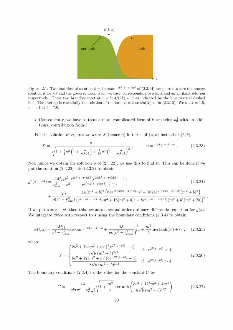
Figure 2.1: Two branches of solution ϕ = 4 arctan e±k(z−vt)±δ of (2.3.14) are plotted where the orangesolution is for +k and the green solution is for −k case, corresponding to a kink and an antikink solutionrespectively. These two branches meet at z = ln 4/(2k) + vt as indicated by the blue vertical dashedline. The overlap is essentially the solution of the form ϕ = 2 arcsin(X) as in (2.3.10). We set k = 1.5,v = 0.1 at t = 7.0.
• Consequently, we have to treat a more complicated form of k replacing k20 with an addi-
tional contribution from b.
For the solution of ψ, first we write X (hence u) in terms of z, v instead of z, v.
X = u√1 + 1
2u2(1 + b
m2+b
)+ 1
16u4(1 − b
m2+b
)2, u = e±k(z−vt)±δ . (2.3.23)
Now, since we obtain the solution ϕ of (2.3.22), we use this to find ψ. This can be done if weput the solution (2.3.22) into (2.3.2) to obtain
g′′(z − vt) = 4M21k2
v2elas − v2
e±k(z−vt)±δ(e2(±k(z−vt)±δ) − 1)(e2(±k(z−vt)±δ) + 1)2 (2.3.24)
+ 2λρ(v2 − v2
elas)±k(m2 + b)2
(64e6(±k(z−vt)±δ)m4 − 1024e2(±k(z−vt)±δ)(m2 + b)2
)(e4(±k(z−vt)±δ)m4 + 16(m2 + b)2 + 8e2(±k(z−vt)±δ)(m2 + b)(m2 + 2b)
)2 .If we put s = z − vt, then this becomes a second-order ordinary differential equation for g(s).We integrate twice with respect to s using the boundary conditions (2.3.4) to obtain
ψ(t, z) = 4M21v2 − v2
elasarctan e±k(z−vt)±δ + 4λ
ρk(v2 − v2elas)
√1 + m2
bacrtanh(Y ) + C , (2.3.25)
where
Y =
8b2 + 12bm2 +m4(1
4e2k(z−vt) + 4)
8√b (m2 + b)3/2
if e2k(z−vt) < 4 ,
8b2 + 12bm2 +m4(4e−2k(z−vt) + 4)8√b (m2 + b)3/2
if e2k(z−vt) > 4 .(2.3.26)
The boundary conditions (2.3.4) fix the value for the constant C by
C = − 4λρk(v2 − v2
elas)
√1 + m2
bacrtanh
(8b2 + 12bm2 + 4m4
8√b (m2 + b)3/2
). (2.3.27)
20
Using the restriction λϕ ≪ 1 and µϕ ≪ 1, the solutions (2.3.22) and (2.3.25) reduce to thesolutions we obtained in [39]
ϕ0 = 4 arctan e±k0(z−vt)±δ
ψ0 = 4M21v2 − v2
elasarctan e±k0(z−vt)±δ .
(2.3.28)
k=1.0 k=3.0 k=6.0 k=1.0 k=3.0 k=6.0
k=1
k=3
k=6
Microrotations Macro displacements
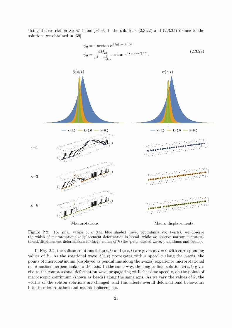
Figure 2.2: For small values of k (the blue shaded wave, pendulums and beads), we observethe width of microrotational/displacement deformation is broad, while we observe narrow microrota-tional/displacement deformations for large values of k (the green shaded wave, pendulums and beads).
In Fig. 2.2, the soliton solutions for ϕ(z, t) and ψ(z, t) are given at t = 0 with correspondingvalues of k. As the rotational wave ϕ(z, t) propagates with a speed v along the z-axis, thepoints of microcontinuum (displayed as pendulums along the z-axis) experience microrotationaldeformations perpendicular to the axis. In the same way, the longitudinal solution ψ(z, t) givesrise to the compressional deformation wave propagating with the same speed v, on the points ofmacroscopic continuum (shown as beads) along the same axis. As we vary the values of k, thewidths of the soliton solutions are changed, and this affects overall deformational behavioursboth in microrotations and macrodisplacements.
21
The soliton solutions for both rotations and displacements were obtained from the equationsof motion, and these allowed us to understand the geometric interpretation of the deformationwaves. Physically dominant parameters of the complete model in determining the overall be-haviour of deformational soliton wave are the Lamé parameters λ, µ and the Cosserat couplemodulus µc. This fact becomes evident by looking at the k dependency, or equivalently mdependency, of the soliton solutions on these parameters.
The various values for k in the soliton solutions for ϕ and ψ give different overall behaviourswhile other values of parameters are fixed. Regarding the microrotations, the effect becomesapparent for large values of k, which induces high-frequency of localised energy distributionon the narrow-width affected cross section both for the microrotational and displacement de-formations, whereas small values of k induce gradual and broad energy distribution for thedeformations over the microcontinuum media. The role of k can be understood using a simplemodel of beads and pendulums as shown in Fig. 2.2.
In the remaining part of this Chapter, we would like to consider some properties of thesolution and its behaviours in limiting cases.
2.4 Properties of solutions
We notice that there might be possible singularity issues in the amplitude of ψ(z, t) in (2.3.25)as v2 approaches v2
elas. Similar situation arose in case of ϕ(z, t) in the value of b, but thishas been resolved by a simple transformation (2.3.9). In order to resolve the current problem,we would like to look closely at k as a function of v taking account of all nine parameters,κ1, κ3, χ1, χ3, ρ, ρrot, µc, λ, µ. We will see that the values for v are restricted to certain rangesfor a given k, so we might expect that this would resolve the singularity problem. This is tospecify a profile of v in terms of k which is often seen in dispersion relations.
We consider only positive roots of k2 of (2.3.21) to understand the possible range of k for agiven v. After putting all relevant parameters in (2.3.21), we obtain
k = 3(
λ2 + (λ+ 2µ− v2ρ)µc
3(λ+ 2µ− v2ρ)(κ1 + 6κ3) − 9v2ρrot(λ+ 2µ− v2ρ) − (3χ1 − χ3)2
)1/2
= 3√ρρrot
(λ2 + µcρ(v2
elas − v2)v4 − (v2
elas + v2rot)v2 + (v2
elasv2rot −M12M21)
)1/2
.
(2.4.1)
Now, to determine whether k possesses any singularity, we compute the discriminant of thequartic of v in the denominator regarding it as a quadratic equation for v2.
(v2elas + v2
rot)2 − 4(v2elasv
2rot −M12M21) = (v2
elas − v2rot)2 + 16ρrot
ρv4
χ , (2.4.2)
where we put v2χ ≡ M12. The expression (2.4.2) is strictly non-negative, so that we can have
four possible roots of v in the denominator of (2.3.28), which will cause the singularity of k.We denote four distinct roots as vi, i = 1, 2, 3, 4, and assume that v1 < v2 < 0 < v3 < v4. Inparticular, we write explicitly
v2 = 12
((v2
elas + v2rot) ±
√(v2
elas − v2rot)2 + 16ρrot
ρv4
χ
). (2.4.3)
The square root of this gives the four roots of vi where two positive roots v3 and v4 are relatedto two negative roots v1 and v2 by v3 = −v2 and v4 = −v1.
22
It can be recognised immediately that the values of velas and vrot are restricted by
v1 ≤ −velas,−vrot ≤ v2 and v3 ≤ velas, vrot ≤ v4 .
Also, we will have k = 0 if v becomes
v20 ≡ (λ2/ρµc) + v2
elas . (2.4.4)
Now, we plot the profiles of v as a function of k and we consider only the positive values ofv for the sake of simplicity. At this time, we only have two asymptotic lines of v3 and v4 (againwe assume v3 < v4). And we assume that velas > vrot.
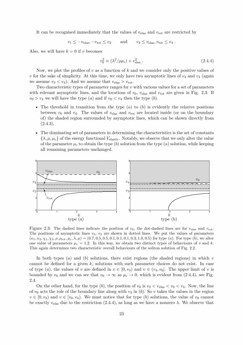
Two characteristic types of parameter ranges for v with various values for a set of parameterswith relevant asymptotic lines, and the locations of v0, velas and vrot are given in Fig. 2.3. Ifv0 > v4 we will have the type (a) and if v0 < v4 then the type (b).
• The threshold in transition from the type (a) to (b) is evidently the relative positionsbetween v0 and v4. The values of velas and vrot are located inside (or on the boundaryof) the shaded region surrounded by asymptotic lines, which can be shown directly from(2.4.3).
• The dominating set of parameters in determining the characteristics is the set of constantsλ, µ, µc of the energy functional Velastic. Notably, we observe that we only alter the valueof the parameter µc to obtain the type (b) solution from the type (a) solution, while keepingall remaining parameters unchanged.
0 1 2 3 40
2
6
8
0 1 2 3 40
2
6
8
type (a) type (b)
Figure 2.3: The dashed lines indicate the position of v0, the dot-dashed lines are for velas and vrot.The positions of asymptotic lines v3, v4 are shown in dotted lines. We put the values of parameters(κ1, κ3, χ1, χ3, ρ, ρrot, µc, λ, µ) = (0.7, 0.5, 0.5, 0.1, 0.1, 0.1, 0.3, 1.0, 0.5) for type (a). For type (b), we alterone value of parameters µc = 1.2. In this way, we obtain two distinct types of behaviours of v and k.This again determines two characteristic overall behaviours of the soliton solution of Fig. 2.2.
In both types (a) and (b) solutions, there exist regions (the shaded regions) in which vcannot be defined for a given k, solutions with such parameter choices do not exist. In caseof type (a), the values of v are defined in v ∈ [0, v3) and v ∈ (v4, v0]. The upper limit of v isbounded by v0 and we can see that v0 → ∞ as µc → 0, which is evident from (2.4.4), see Fig.2.4.
On the other hand, for the type (b), the position of v0 is v3 < velas < v0 < v4. Now, the lineof v0 acts the role of the boundary line along with v3 in (b). So v takes the values in the regionv ∈ [0, v3) and v ∈ [v0, v4). We must notice that for type (b) solutions, the value of v0 cannotbe exactly velas due to the restriction (2.4.4), as long as we have a nonzero λ. We observe that
23
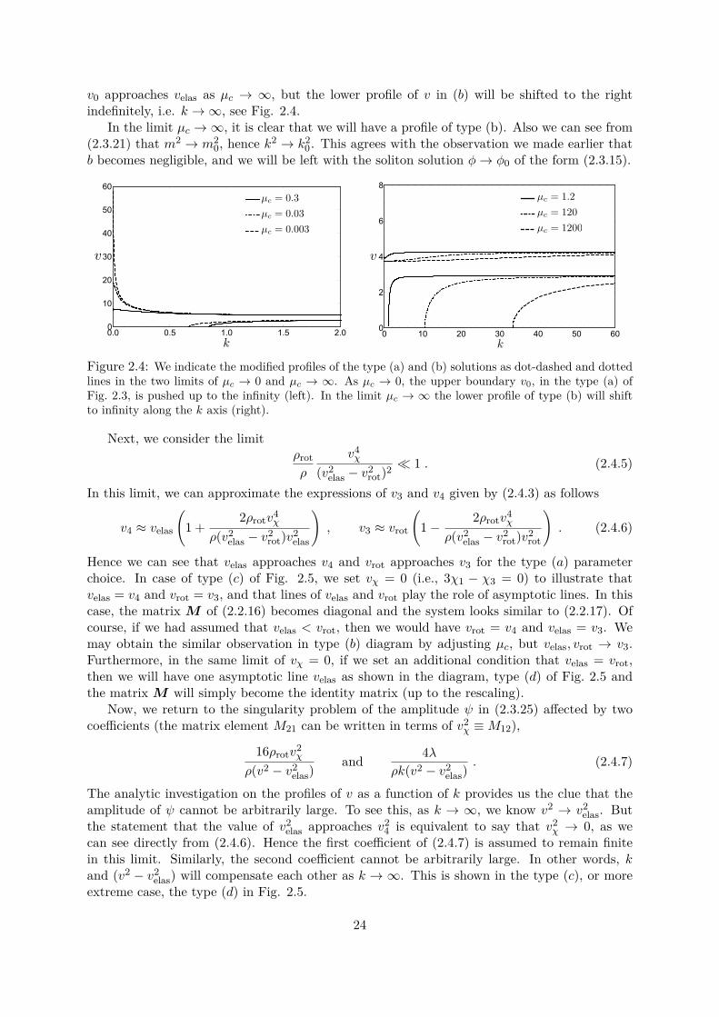
v0 approaches velas as µc → ∞, but the lower profile of v in (b) will be shifted to the rightindefinitely, i.e. k → ∞, see Fig. 2.4.
In the limit µc → ∞, it is clear that we will have a profile of type (b). Also we can see from(2.3.21) that m2 → m2
0, hence k2 → k20. This agrees with the observation we made earlier that
b becomes negligible, and we will be left with the soliton solution ϕ → ϕ0 of the form (2.3.15).
0.0 0.5 1.0 1.5 2.00
10
20
30
40
50
60
0 10 20 30 40 50 600
2
4
6
8
Figure 2.4: We indicate the modified profiles of the type (a) and (b) solutions as dot-dashed and dottedlines in the two limits of µc → 0 and µc → ∞. As µc → 0, the upper boundary v0, in the type (a) ofFig. 2.3, is pushed up to the infinity (left). In the limit µc → ∞ the lower profile of type (b) will shiftto infinity along the k axis (right).
Next, we consider the limitρrotρ
v4χ
(v2elas − v2
rot)2 ≪ 1 . (2.4.5)
In this limit, we can approximate the expressions of v3 and v4 given by (2.4.3) as follows
v4 ≈ velas
(1 +
2ρrotv4χ
ρ(v2elas − v2
rot)v2elas
), v3 ≈ vrot
(1 −
2ρrotv4χ
ρ(v2elas − v2
rot)v2rot
). (2.4.6)
Hence we can see that velas approaches v4 and vrot approaches v3 for the type (a) parameterchoice. In case of type (c) of Fig. 2.5, we set vχ = 0 (i.e., 3χ1 − χ3 = 0) to illustrate thatvelas = v4 and vrot = v3, and that lines of velas and vrot play the role of asymptotic lines. In thiscase, the matrix M of (2.2.16) becomes diagonal and the system looks similar to (2.2.17). Ofcourse, if we had assumed that velas < vrot, then we would have vrot = v4 and velas = v3. Wemay obtain the similar observation in type (b) diagram by adjusting µc, but velas, vrot → v3.Furthermore, in the same limit of vχ = 0, if we set an additional condition that velas = vrot,then we will have one asymptotic line velas as shown in the diagram, type (d) of Fig. 2.5 andthe matrix M will simply become the identity matrix (up to the rescaling).
Now, we return to the singularity problem of the amplitude ψ in (2.3.25) affected by twocoefficients (the matrix element M21 can be written in terms of v2
χ ≡ M12),
16ρrotv2χ
ρ(v2 − v2elas)
and 4λρk(v2 − v2
elas). (2.4.7)
The analytic investigation on the profiles of v as a function of k provides us the clue that theamplitude of ψ cannot be arbitrarily large. To see this, as k → ∞, we know v2 → v2
elas. Butthe statement that the value of v2
elas approaches v24 is equivalent to say that v2
χ → 0, as wecan see directly from (2.4.6). Hence the first coefficient of (2.4.7) is assumed to remain finitein this limit. Similarly, the second coefficient cannot be arbitrarily large. In other words, kand (v2 − v2
elas) will compensate each other as k → ∞. This is shown in the type (c), or moreextreme case, the type (d) in Fig. 2.5.
24

0 1 2 3 40
2
4
6
8
0 1 2 3 40
2
4
6
8
type (c) type (d)
Figure 2.5: For (c), we put (κ1, κ3, χ1, χ3, ρ, ρrot, µc, λ, µ) = (0.7, 0.5, 0.5, 1.5, 0.1, 0.1, 0.3, 1.0, 0.5) sothat 3χ1 − χ3 = 0 and we obtain v4 = velas = 4.47214 and v3 = vrot = 3.51188. For (d), we only alteredvalue of parameter κ1 = 3.0 so that velas = vrot = v3 = v4 = 4.47214.
2.5 Galilean transformations and Lorentzian transformationsIf a given system is invariant under certain symmetry, then we can apply the same symmetryto a solution of the Euler-Lagrangian equation from the system to see whether the symmetryremain valid or not. This gives us a clue about the nature of solution space. For example,suppose we have a system of scalar field ϕ(z, t) with a Lagrangian
L = 12
(∂ϕ
∂t
)2− 1
2
(∂ϕ
∂z
)2− U(ϕ) (2.5.1)
for some potential U(ϕ). The equation of motion can be obtained by(∂2
∂t2− ∂2
∂z2
)ϕ = −∂U
∂ϕ. (2.5.2)
We can write total energy H defined by an integration of energy density H over all space,
H =∫dz H
=∫dz
[12
(∂ϕ
∂t
)2+ 1
2
(∂ϕ
∂z
)2+ U(ϕ)
],
(2.5.3)
where energy density H in terms of conjugate momentum π = ∂L/∂ϕ is defined by
H = πϕ− L . (2.5.4)
Now, if we consider a static case in evaluating the solution, we have
∂2ϕ
∂z2 = ∂U
∂ϕ. (2.5.5)
In particular, if we have the potential U given by
U(ϕ) = 14(ϕ2 − 2m2
)2,
then the solution is the well-known form of a pair of kink and antikink soliton solutions subjectto boundary conditions similar to (2.3.4),
ϕ(z) = ±√
2m tanh(√
m2 z). (2.5.6)
25
Further, we impose that the Lagrangian is invariant under the Lorentz transformation. Thismeans that if we apply the same transformation to the wave equation we obtained, it will stillremain as a valid solution to the given system. This is a widely known technique in solving atime-dependent partial differential equation from its static case [40], when a certain symmetrygroup for the Lagrangian is identified, and applicable to the static solution. We would liketo emphasise here that the same method can be applied in our solution, by noting that theGalilean transformation is a limiting case of the Lorentz transformation.
Now, if we apply the Lorentz boost (the Lorentz transformation in one direction) to thestatic wave solution (2.5.6) along, say the z-axis, then what we can expect is that the wavepacket starts moving in the direction along the transformation applied with a nonzero velocity.Hence a time-dependent wave solution for (2.5.2) is simply
ϕ(z, t) = ±√
2m tanh
√ m2
1 − v2 (z − vt)
, (2.5.7)
in which z is replaced by (z− vt)/√
1 − v2, according to the Lorentz boost along the z-axis (weput the speed of light c = 1),
t′ = t− v/c2z√1 − v2/c2 , z′ = z − vt√
1 − v2/c2 , x′ = x , y′ = y . (2.5.8)
For our case of the soliton solution for the microrotation governed by ϕ, suppose we havestarted with a static case with an equation of motion, instead of the full dynamic case (2.3.7),
− ∂2ϕ
∂z2 +m2 sinϕ+ b
2 sin 2ϕ = 0 , (2.5.9)
in which we dropped the hat for the rescaled quantities for now. It is easy to check that thesolution for this is of the form,
ϕ(z) = 2 arcsin(X(z)) (2.5.10)
with the identical form X of (2.3.11), but now the static function u in X is
u(z) = exp[√
m2 + b z]. (2.5.11)
If we apply the Lorentz boost in the z-axis to this static solution, then the time-dependentsoliton solution would be (2.3.10) with
u(z, t) = exp
√m2 + b
1 − v2 (z − vt) ± δ
, (2.5.12)
which agrees with the solution we obtained in (2.3.10).Of course, the key ingredient in facilitating the analysis we used in solving the coupled
system given in (2.2.15) is strictly based on the dynamic assumption that the displacementwave propagation satisfies (2.3.1),
∂ttψ = v2∂zzψ ,
and the underlying symmetry in the energy functional is the global Galilean transformationwith the speed of light is taken to be c → ∞ in (2.5.8)
t′ = t , z′ = z − vt , x′ = x , y′ = y . (2.5.13)
26
However, we would like to emphasise the fact that the equation of motion and its soliton solutionfor the microrotation we obtained is well compatible with the system which contains the Lorentztransformation as its fundamental symmetry group, once one identifies the equation of motioncan be derived to the form of (2.3.7).
This also signifies the effect and its validity of applying the Lorentz boost to the staticsolution to obtain the time-dependent solution, when the soliton solution describes the particle-like isolated behaviour prevented from any possible interference from undesired interaction tolose its solitonic character, in particular when one considers the multi-soliton system. This isexactly the case when we have k → ∞ in (2.3.21), see Fig. 2.2, in our soliton solution ϕ of(2.3.22).
27

28
Chapter 3
Chiral energy
3.1 Chiralities in continua
A group of geometric symmetries which keeps at least one point fixed is called a point group.A point group in N -dimensional Euclidean space is a subgroup of the orthogonal group O(N).Naturally this leads to the distinction of rotations and improper rotations. Centrosymmetrycorresponds to a point group which contains an inversion centre as one of its symmetry elements.Chiral symmetry is one example of non-centrosymmetry which is characterised by the fact thata geometric figure cannot be mapped into its mirror image by an element of the Euclideangroup, proper rotations SO(N) and translations. We denote this property as chirality, andquantities responsible for this property by chiral terms.
This non-superimposability (i.e. chirality) to its mirror image is best illustrated by the leftand right hands. There is no way to map the left hand onto the right by simply rotating the lefthand in the plane. And there is no mirror symmetry line within one hand to map into another.This geometrical feature of chirality can be found in many molecules which can have distinctchemical properties. A fairly stable or harmless substance can have an unstable or noxioussubstance as its chiral counterpart [41].
If one applies the Lorentz boost discussed in Section 2.5 to a spinning particle in its mo-mentum direction in one frame of reference, while retaining its spin orientation, this will causean opposite direction of momentum to another frame of reference. This discrete symmetry isknown as parity and leads to the notion of left or right-handedness in particle physics.
In continuum mechanics, it is often observed that chiral materials in three-dimensionalspace lose their chirality [42–44] when projected into a two-dimensional plane. A linear energyfunction (quadratic energy in small strains) for an isotropic material in the centrosymmetriccase was studied in [10], and the absence of odd-rank isotropic tensors implicitly implied thelack of material parameters for the non-centrosymmetric case. Similar works [42,45] consideredan energy function which contains a fourth order isotropic tensor with chiral coupling terms byidentifying axial tensors as being asymmetric under the inversion. When one attempts to applythese ideas to the planar case, the chiral coupling term turns out to vanish [43, 44], and onearrives at an isotropic (and centrosymmetric) model without chirality.
A rank-five isotropic tensor is introduced in [46] to impose chirality on the energy containinga single chiral material parameter. This type of chirality is related to the gradient of rotation,which led to the existence of torsion. Based on the assertion that hyperelastic Cosserat materialsare hemitropic, invariant under the right action of SO(3), if and only if the strain energy ishemitropic, a set of hemitropic strain invariants can be found in [47]. Many attempts weremade to understand the mechanism behind the loss of chirality, and in constructing a generictwo-dimensional chiral configuration without referring to higher dimensions. A chiral rank-four
29
isotropic tensor is used in [44] to derive a chiral material constant in the equations of motion,and in subsequent works [48,49] the two-dimensional chirality problem is further considered. Aplanar micropolar model is proposed in [50] with the help of the irreducible decomposition ofgroup representation.
Recent growing interests of planar chirality [51–55] concerns the polarised propagation ofelectromagnetic waves. The optical behaviour indicates that planar chirality behaves differ-ently from its three-dimensional counterpart. In [56] a two-dimensional chiral optical effect innanostructure is studied in comparison with three-dimensional chirality. The two-dimensionalmicropolar continuum model of a chiral auxetic lattice structure in connection with negativePoisson’s ratio is discussed in [43,50,57,58]. The theoretical analysis of planar chiral lattices iscompared with experimental results in [59].
A schematic description of chiral transformations and changes of the number of symmetrygroups from higher dimensions (macroscale chiral layers) to lower dimensions (molecules of chiralline structure) is outlined in [60], backed by various experimental results. Further developmentsin three-dimensional chiral structures can be found in [61–63].
Let us begin with an immediate observation regarding the rotational field in line of our inter-ests. In three-dimensional space it is in general non-Abelian, while it may become Abelian groupstructure in lower dimensions. So, a certain loss of information is expected when projecting tolower dimensional space.
In this Chapter, we will construct a new geometrically nonlinear energy term which isexplicitly chiral in three dimensions, and which does not lose this character when applied tothe planar problem. This will shed light in understanding the genuine property of energy termswhich gives rise to chirality in various models.
We would like to introduce the so-called first planar Cosserat problem briefly here. Thedisplacement vector is given by u = (u1, u2, 0) while planar rotations are described by a rotationaxis n = (0, 0, n3). Then the dislocation density tensor (2.1.5) defined by
K = RT CurlR
is nonzero. Since the microrotations are described by the orthogonal matrix R ∈ SO(3), it doescontain a 2×2 zero block matrix in the planar indices. This induces several orthogonal relations,for example, with the first Cosserat deformation tensor U = R
TF , which makes it impossible
to construct coupling terms in the energy which do not vanish identically in the plane, see thedetailed discussions in [24,64].
Let us illustrate a simple example regarding chirality in three dimensions which can be trans-lated into two dimensions. In Fig. 3.1, two chiral dice are given which cannot be SO(3)-rotatedto superimpose onto each other in three dimensions on the top, and two chiral hexagons aregiven which again cannot be SO(2)-rotated to superimpose onto each other in two dimensionson the bottom. In the middle, there are two specific procedures to preserve the chirality fromthree dimensions when projected to two dimensions. One of them is the way of labelling thenumber of dots on the chiral dice to be projected to the chiral hexagon, and another is to specifythe choice of perspective.
This example suggests, at least at an intuitive level, that one can construct a three-dimensionalchiral structure and a projection, such that the resulting two-dimensional structure inherits thechirality in a certain way. However we must note that if we had a different way of labellingdots on the chiral dice or with a different choice of perspective, we would not find a chiralhexagon on the plane. In other words, the chirality preservation through the projection intothe lower-dimensional space depends critically on its construction.
30
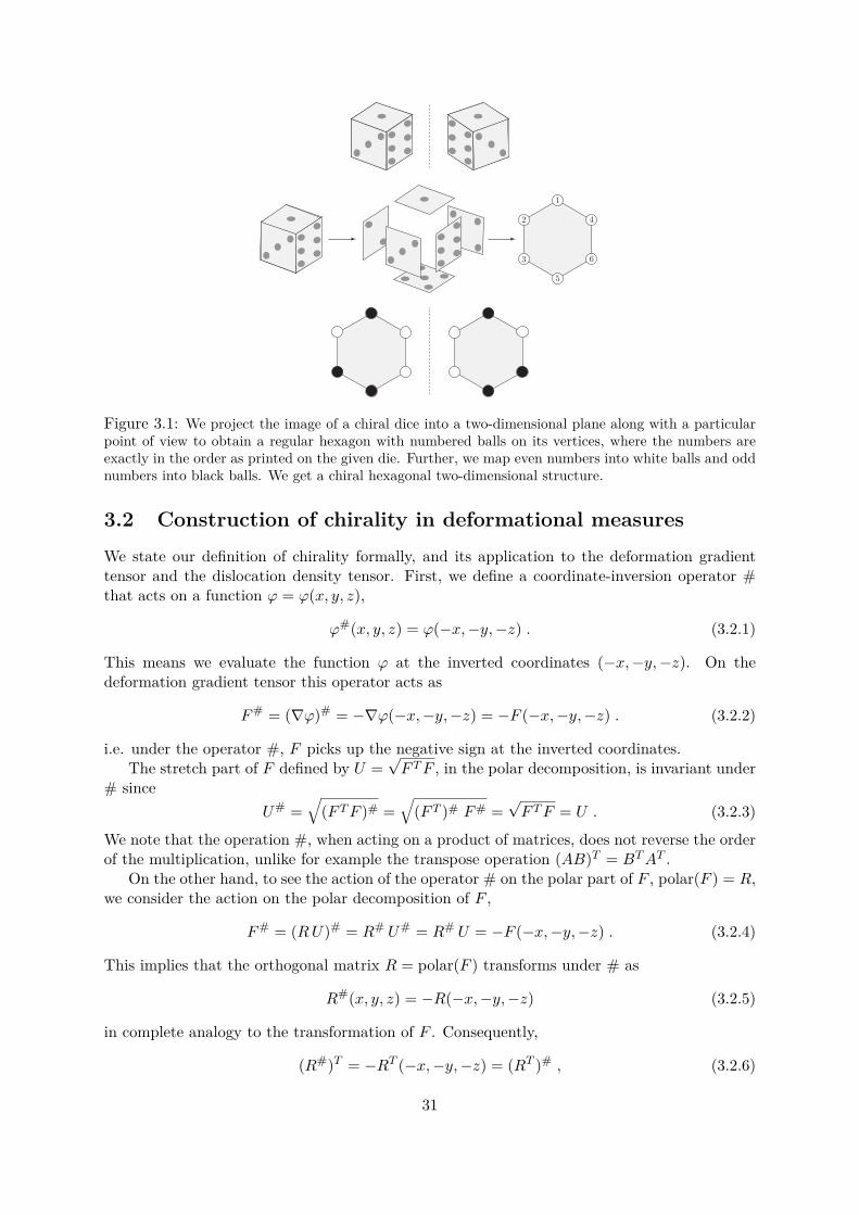
Figure 3.1: We project the image of a chiral dice into a two-dimensional plane along with a particularpoint of view to obtain a regular hexagon with numbered balls on its vertices, where the numbers areexactly in the order as printed on the given die. Further, we map even numbers into white balls and oddnumbers into black balls. We get a chiral hexagonal two-dimensional structure.
3.2 Construction of chirality in deformational measuresWe state our definition of chirality formally, and its application to the deformation gradienttensor and the dislocation density tensor. First, we define a coordinate-inversion operator #that acts on a function φ = φ(x, y, z),
φ#(x, y, z) = φ(−x,−y,−z) . (3.2.1)
This means we evaluate the function φ at the inverted coordinates (−x,−y,−z). On thedeformation gradient tensor this operator acts as
F# = (∇φ)# = −∇φ(−x,−y,−z) = −F (−x,−y,−z) . (3.2.2)
i.e. under the operator #, F picks up the negative sign at the inverted coordinates.The stretch part of F defined by U =
√F TF , in the polar decomposition, is invariant under
# sinceU# =
√(F TF )# =
√(F T )# F# =
√F TF = U . (3.2.3)
We note that the operation #, when acting on a product of matrices, does not reverse the orderof the multiplication, unlike for example the transpose operation (AB)T = BTAT .
On the other hand, to see the action of the operator # on the polar part of F , polar(F ) = R,we consider the action on the polar decomposition of F ,
F# = (RU)# = R# U# = R# U = −F (−x,−y,−z) . (3.2.4)
This implies that the orthogonal matrix R = polar(F ) transforms under # as
R#(x, y, z) = −R(−x,−y,−z) (3.2.5)
in complete analogy to the transformation of F . Consequently,
(R#)T = −RT (−x,−y,−z) = (RT )# , (3.2.6)
31
which means that F (or F T ) and its polar part R (or RT ) transform in the same way under #.There is a deep meaning of acquiring the additional minus sign when one applies the inver-
sion # to the rotation, in particular, if one takes the rotation R such as (2.2.1) with a fixedrotational axis. For example, if we consider the general rotational representation (1.2.31), thetransformation properties of a general rotational matrix under inversion can be understoodquite naturally. Consider the transformation from the reference configuration XL to the spatialconfiguration xi = RiLXL by a rotation
RiL = δiL cosϕ+ ϵijLnj sinϕ+ (1 − cosϕ)ninL (3.2.7)
where ni is an axis of rotation and ϕ is a rotational angle in spatial configuration. nL is anaxial vector in the reference configuration. Then applying the inversion operator # gives
R#iL = −δiL cosϕ− ϵijLnj sinϕ− (1 − cosϕ)ninL , (3.2.8)
in which δiL acquires a negative sign in the spatial configuration, and ni changes its directionunder the inverted coordinates but nL remains unaffected in the reference configuration. Thisagrees with result (3.2.5). More generally speaking, for R ∈ O(3), we have detR = ±1 and wecan write
R = s eA , detR =
+1 if s = +1 ,−1 if s = −1 ,
(3.2.9)
where A is a 3 × 3 skew-symmetric matrix. This classification identifies the relation betweenR ∈ SO(3) and its chiral counterpart R#. If detR = +1 we have detR# = −1, and viceversa. We note that these arguments are valid not only in case of macrorotations, but also inmicrorotations in which the relations are defined by (1.2.25) in terms of directors.
On an equal footing, the deformation gradient tensor is defined by FiR = ∂xi∂XR
for xi =Xi + ui(Xk), and applying the operator # gives
F#iR = ∂(−xi)
∂XR= −FiR , (3.2.10)
also in agreement with (3.2.4).Now, consider the operation Curl of (2.1.4) on R#,
(CurlR#)ij = ϵjkl∂kR#il . (3.2.11)
It is easy to observe that each partial derivative gives additional minus signs to the matrixelements of R# using the chain rule, for instance
∂yR# = −∂yR(−x,−y,−z) = ∂−yR(−x,−y,−z) = (∂yR)(−x,−y,−z) (3.2.12)
so that the partial derivative of R with respect to y is evaluated in the usual Cartesian coordi-nates, but the quantity ∂yR is viewed in the inverted coordinate system (−x,−y,−z). Then
Curl (R#)(x, y, z) = (CurlR)(−x,−y,−z) . (3.2.13)
Hence, we see that the operator Curl negates the minus sign obtained when # is acted onR. But we can easily construct a deformational measure which transforms like (3.2.4). Thedislocation density tensor is such an example, satisfying
(RT CurlR)# = (R#)T CurlR# = −(RT CurlR)(−x,−y,−z) . (3.2.14)
32
It is no coincidence that the dislocation density tensor is exactly of this form. Clearly, we willarrive at the same conclusions for R = polar(F ) and F ∈ GL(3; R)
F#(x, y, z) = −F (−x,−y,−z) , (3.2.15a)
R#(x, y, z) = −R(−x,−y,−z) , (3.2.15b)
K# = (RT CurlR)#(x, y, z) = −(RT CurlR)(−x,−y,−z) = −K . (3.2.15c)
In this way, we would like to investigate some frequently appearing matrix quantities in theCosserat elasticity energy functional, accompanied by conventional matrix operations such astranspose, trace or Frobenius scalar product. We will see whether they are chiral or not. Thiswill lead to a simple combination of products which yields a chiral energy functional.
3.3 Constructing chiral energy functionalsWe show the construction of one possible chiral term which can form the building blocks inconstructing a multitude of other chiral terms. In searching for a generic objective [65] andchiral term for a chiral energy functional, we begin by recalling objectivity.
We call an energy functional objective if it is invariant under the left-action of global rotationsQ with detQ = +1, here Q ∈ SO(3) is a constant position-independent orthogonal matrix.Under the global rotation of Q on F and R, respectively, we have
F = RU −→ QF = QRU and R −→ QR . (3.3.1)
It is easy to verify that the dislocation density tensor K is objective, under the global rotationQ acting on R
K = RT CurlR −→ (QR)T Curl (QR) = R
TQTQCurlR = K . (3.3.2)
Therefore, K is objective and also chiral quantity due to (3.2.15c).These observations allow us to construct two additional terms which are both objective and
chiral quantities from which we wish to use in constructing the chiral energy term, namely
L = RT CurlR and M = RT CurlR . (3.3.3)
Here, again, R is the orthogonal part of the polar decomposition, while R is the microrotation.In principle one could also consider the term K = RT CurlR.
Now, we have a set of chiral and objective terms at our disposal
K,K,L,M,KT,KT , LT ,MT , · · · , (3.3.4)
from which we can construct a chiral energy functional. We note that a product of an oddnumber of chiral terms is required to preserve chirality.
In addition to the notion of objectivity, an energy functional is hemitropic if it is invari-ant under right-action of global rotations excluding inversions, i.e. right-invariant under theelements of SO(3) [65]. In particular, the invariance under the right-action of O(3) is calledisotropy. Considering the (right) rotation Q2 ∈ SO(3), we find that F and R transform as
F = RU −→ RQ2U and R −→ RQ2 . (3.3.5)
This implies the following property
K = RT CurlR −→ (RQ2)T Curl (RQ2) = QT
2 RT CurlRQ2 = QT
2 KQ2 . (3.3.6)
33
Likewise, we find
L = RT CurlR −→ (RQ2)T CurlRQ2 = QT2 LQ2 ,
M = RT CurlR −→ (RQ2)T CurlRQ2 = QT
2 MQ2 .(3.3.7)
Finally, we consider the energy functional
Vχ = χtr(K K K
), χ ∈ R . (3.3.8)
We note its three main properties as follows.
1. K is invariant under the left action of SO(3), hence Vχ is invariant under the left actionof SO(3), thus it is objective.
2. K is chiral, Vχ is odd in K and hence Vχ is chiral, V #χ = −Vχ.
3. Vχ is invariant under the right action of SO(3), so it is hemitropic. This is because
Vχ = χtr(K K K
)−→ χtr
(QT
2 KQ2QT2 KQ2Q
T2 KQ2
)= χtr
(QT
2 K K KQ2)
= Vχ ,
due to the cyclic property of the trace.
This means Vχ is objective, hemitropic and chiral. Clearly, following the same approach, onecan consider similarly structured terms based on cubic combinations of K, L and M . For thesake of simplicity, we will focus on the easiest of these terms.
3.4 Variations of a chiral equationThe chiral energy term Vχ is by no means guaranteed to lead to a non-vanishing contributionto the equations of motion when the planar problem is considered. However, it will turn outto produce the necessary terms to preserve planar chirality. In the following we will define anenergy functional from which we will derive equations of motions. After constructing an explicitsolution, we will discuss the chiral properties of the solution.
Let us begin by defining the total energy functional now including a chiral term Vχ of theform (3.3.8) for the Cosserat material which is given by
V = Velastic(F,R) + Vcurvature(R) + Vχ(R) − Vkinetic(u, R) , (3.4.1)
where the individual terms are
Velastic(F,R) = µ∥∥∥sym(RT
F − 1)∥∥∥2
+ λ
2[tr(sym(RT
F − 1))]2
(3.4.2a)
Vcurvature(R) = κ1∥∥∥dev sym(RT CurlR)
∥∥∥2+ κ2
∥∥∥skew(RT CurlR)∥∥∥2
+ κ3[tr(RT CurlR)
]2(3.4.2b)
Vχ(R) = χtr(K K K
)(3.4.2c)
Vkinetic = 12ρ∥u∥2 + ρrot∥R∥2 . (3.4.2d)
Following the results from Chapter 2, the variation of the total energy functional
δV = δVelastic(F,R) + δVcurvature(R) + δVχ(R) − δVkinetic(u, R) (3.4.3)
34
will lead to the equations of motion by collecting corresponding terms of δR and δF separately.The detailed calculations for varying functionals Velastic and Vcurvature are given in Appendix A.The variation of Vχ can also be found in Appendix A and we write these variational terms,
δVelastic(F,R) =[µ(RF TR+ F ) − (2µ+ 3λ)R+ λtr(RT
F )R]
: δF
+[µFR
TF − (2µ+ 3λ)F + λtr(RT
F )F]
: δR+ ρu δu (3.4.4a)
δVcurvature(R) =[(κ1 − κ2)
((CurlR)RT (Curl (R)) + Curl
[R(CurlR)TR
])+ (κ1 + κ2)Curl
[CurlR
]−(κ13 − κ3
)(4tr(RT CurlR)Curl (R) − 2R
(grad
(tr[RT CurlR]
))⋆+ 2ρrotR
]: δR
(3.4.4b)
δVχ = 3χ[(CurlR)(K2) + Curl [R(K2)T ]
]: δR . (3.4.4c)
Collecting δF terms gives 3 × 3 matrix A
µ(RF TR+ F ) − (2µ+ 3λ)R+ λtr(RTF )R = A . (3.4.5)
As we did in Chapter 2, the δF terms are evaluated using the fact
A : δF = AijδFij −→ −∂jAijδui = − (∂1A31 + ∂2A32 + ∂3A33) δψ ,
for any matrix A, where a total derivative term was neglected.Likewise, collecting δR terms from these variations can be summarised to a single matrix
B as shown in the following
3χ[(CurlR)(K2) + Curl [R(K2)T ]
]+ µFR
TF −
(2µ+ 3λ
)F + λtr(RT
F )F
+ (κ1 − κ2)((CurlR)RT (Curl (R)) + Curl
[R(CurlR)TR
])+ (κ1 + κ2)Curl
[CurlR
]−(κ1
3 − κ3)(
4tr(RT CurlR)Curl (R)
− 2R[grad
(tr[RT CurlR]
)]⋆)+ 2ρrotR = B . (3.4.6)
3.5 Equations of motion and solutions
Now we are in position to state explicitly the dynamic equations of motion in the plane, andshow that chirality does not vanish. We then solve those equations and explain their chiralstructure. In order to study the equations of motion in the plane, we will make the followingidentical assumptions we used in Chapter 2. These are
1. Material points can only experience rotations about one axis, say the z-axis.
2. Displacements occur along this axis of rotation.
3. Elastic displacement waves and microrotational waves are both longitudinal, and propa-gate with the same constant wave speed v.
Consequently, the microrotation matrix, the displacement vector and deformation gradient ten-sor are exactly identical to (2.2.1) and (2.2.4). This implies F = U and polar(F ) = R = 1.
35
And from these, we can write the explicit forms of the dislocation density tensor K defined byK = R
T CurlR,
K =
∂zϕ 0 00 ∂zϕ 00 0 0
. (3.5.1)
Now, under these assumptions, only the A33 contributes in the δF term, which is given by
A33 = 2λ(cosϕ− 1) + (λ+ 2µ)∂zψ . (3.5.2)
This gives the equation of motion of ψ,
ρ∂ttψ + 2λ sinϕ ∂zϕ− (λ+ 2µ)∂zzψ = 0 . (3.5.3)
On the other hand, the quantity B : δR becomes
B : δR = tr[BT δR] = tr
B11 −B12 0B12 B11 00 0 B33
− sinϕ − cosϕ 0
cosϕ − sinϕ 00 0 0
δϕ
= −(2B11 sinϕ+ 2B12 cosϕ)δϕ .
(3.5.4)
The required components of B are given by
B11 = −2(λ+ µ) + 13 cosϕ
[3(2λ+ µ) − 6ρrot(∂tϕ)2 + (∂zϕ)2(κ1 − 3κ2 + 24κ3 + 18χ∂zϕ)
]+ λ∂zψ + 2
3 sinϕ[−3ρrot∂ttϕ+ (κ1 + 6κ3 + 9χ∂zϕ)∂zzϕ
], (3.5.5a)
B12 = 13 sinϕ
[(3µ+ 6ρrot(∂tϕ)2 − (∂zϕ)2(κ1 − 3κ2 + 24κ3 + 18χ∂zϕ)
]+ 2
3 cosϕ[−3ρrot∂ttϕ+ (κ1 + 6κ3 + 9χ∂zϕ)∂zzϕ
]. (3.5.5b)
Putting everything together gives the equation of motion for ϕ, together with the previousequation for ψ of (3.5.3). This coupled system of equations is given by
ρrot ∂ttϕ−(κ1 + 6κ3
3
)∂zzϕ− 3χ∂zϕ ∂zzϕ+ (λ+ µ)(1 − cosϕ) sinϕ− λ
2 sinϕ ∂zψ = 0 ,
(3.5.6a)ρ ∂ttψ + 2λ sinϕ ∂zϕ− (λ+ 2µ)∂zzψ = 0 .
(3.5.6b)
Now, we seek solutions of the form ϕ = f(z−vt) and ψ = g(z−vt), where v is the same wavespeed for both the elastic and the rotational wave propagation according to our assumptions.This means they both satisfy the wave equations
∂ttf = v2∂zzf and ∂ttg = v2∂zzg .
We introduce a new variable s = z − vt, and denote the differentiation with respect to s bya prime. Putting this ansatz into the equation of motion of ψ (3.5.5b) gives
ρv2g′′ + 2λ sin(f)f ′ − (λ+ 2µ)g′′ = 0 ,
which can be rewritten by
(ρv2 − (λ+ 2µ))g′′ − 2λ sin(f)f ′ = 2λ dds
(cos(f)) . (3.5.7)
36
Since it is reduced to a second-order ordinary differential equation, we can now integrate withrespect to s which gives
g′ = 2λρv2 − (λ+ 2µ) cos(f) + C1 , (3.5.8)
for some constant of integration C1. Since ∂zψ = g′ we can now eliminate this term from theequation of motion (3.5.6a) which becomes
ρrotv2f ′′ −
(κ1 + 6κ3
3
)f ′′ − 3χf ′f ′′ + (λ+ µ)(1 − cosϕ) sinϕ
− λ
2 sin(f)( 2λρv2 − (λ+ 2µ) cos(f) + C1
)= 0 .
(3.5.9)
After rearranging terms, this can be rewritten as follows
ρrotv2f ′′ −
(κ1 + 6κ3
3
)f ′′ − 3χf ′f ′′ +
[(λ+ µ) − λ
2C1
]sin(f)
− 12
[(λ+ µ) + λ2
ρv2 − (λ+ 2µ)
]sin(2f) = 0 .
(3.5.10)
When setting χ = 0, this becomes the double sine-Gordon equation, we saw in Chapter 2 for thesoliton solution we constructed with the line of symmetry passes through the peak of the wavepacket, hence non-chiral. However, with a nonzero chiral parameter χ, there is an additionalcontribution from the non-linearity of the form χf ′f ′′, and this might give the desired result forthe chirality in the solution.
3.6 Constructing approximate solutionsInspection of equation (3.5.10) shows that each of these five terms can be integrated after theentire equation is multiplied by f ′. This yields
12
[ρrotv
2 −(κ1 + 6κ3
3
)](f ′)2 − χ(f ′)3 −
[(λ+ µ) − λ
2C1
]cos(f)
+ 14
[(λ+ µ) + λ2
ρv2 − (λ+ 2µ)
]cos(2f) = C2 ,
(3.6.1)
where C2 is another constant of integration. Formally, this is a cubic equation in f ′ (quadraticin f ′ if χ = 0) which can, in principle, be solved for f ′ and will give three different solutions ingeneral. The resulting equation is always of the general form f ′ = H(f) and is hence separable.
• This means we have reduced finding a solution to our system of nonlinear wave equations(3.5.6a) and (3.5.6b) to an integration problem. Note that this solution depends on theeight parameters v, λ, µ, ρ, κ1, κ3, ρrot, χ and two constants of integration C1 and C2. Ingeneral, these solutions will involve special functions if an explicit solution can be found.
• With nonzero chiral parameter χ, we cannot approach with the analytic method usedin the double sine-Gordon equation. But we will construct an approximated solution to(3.6.1), using a suitable choice of the constants of integration.
The chiral parameter χ is assumed to be small so that a series expansion in this parametercan be made. We choose C1 = 2(λ+ µ)/λ, put F(s) = 2f(s) and choose C2 such that one canwrite
(F ′)2 − χ(F ′)3 = 2m2(1 − cos(F)) (3.6.2)
37
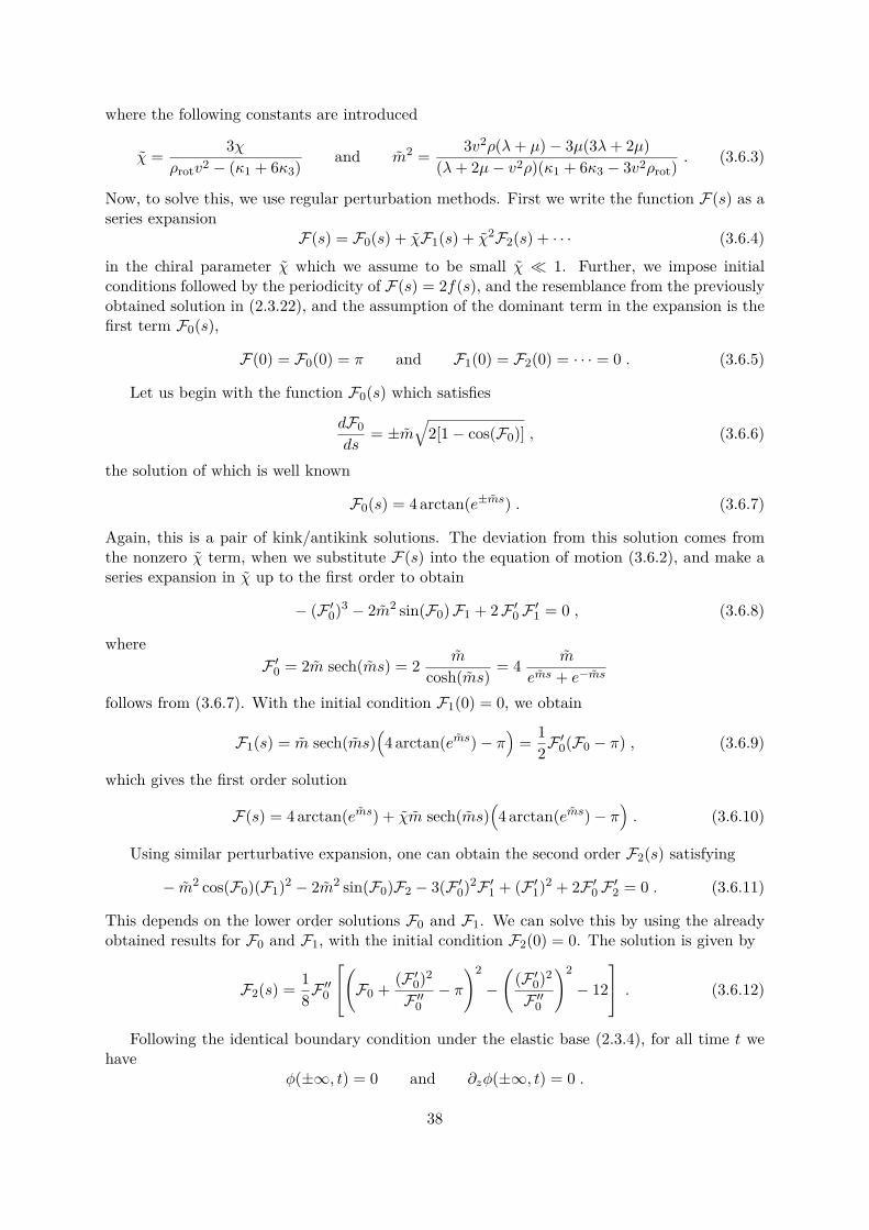
where the following constants are introduced
χ = 3χρrotv2 − (κ1 + 6κ3) and m2 = 3v2ρ(λ+ µ) − 3µ(3λ+ 2µ)
(λ+ 2µ− v2ρ)(κ1 + 6κ3 − 3v2ρrot). (3.6.3)
Now, to solve this, we use regular perturbation methods. First we write the function F(s) as aseries expansion
F(s) = F0(s) + χF1(s) + χ2F2(s) + · · · (3.6.4)in the chiral parameter χ which we assume to be small χ ≪ 1. Further, we impose initialconditions followed by the periodicity of F(s) = 2f(s), and the resemblance from the previouslyobtained solution in (2.3.22), and the assumption of the dominant term in the expansion is thefirst term F0(s),
F(0) = F0(0) = π and F1(0) = F2(0) = · · · = 0 . (3.6.5)
Let us begin with the function F0(s) which satisfies
dF0ds
= ±m√
2[1 − cos(F0)] , (3.6.6)
the solution of which is well known
F0(s) = 4 arctan(e±ms) . (3.6.7)
Again, this is a pair of kink/antikink solutions. The deviation from this solution comes fromthe nonzero χ term, when we substitute F(s) into the equation of motion (3.6.2), and make aseries expansion in χ up to the first order to obtain
− (F ′0)3 − 2m2 sin(F0) F1 + 2 F ′
0 F ′1 = 0 , (3.6.8)
whereF ′
0 = 2m sech(ms) = 2 m
cosh(ms) = 4 m
ems + e−ms
follows from (3.6.7). With the initial condition F1(0) = 0, we obtain
F1(s) = m sech(ms)(4 arctan(ems) − π
)= 1
2F ′0(F0 − π) , (3.6.9)
which gives the first order solution
F(s) = 4 arctan(ems) + χm sech(ms)(4 arctan(ems) − π
). (3.6.10)
Using similar perturbative expansion, one can obtain the second order F2(s) satisfying
− m2 cos(F0)(F1)2 − 2m2 sin(F0)F2 − 3(F ′0)2F ′
1 + (F ′1)2 + 2F ′
0 F ′2 = 0 . (3.6.11)
This depends on the lower order solutions F0 and F1. We can solve this by using the alreadyobtained results for F0 and F1, with the initial condition F2(0) = 0. The solution is given by
F2(s) = 18F ′′
0
(F0 + (F ′0)2
F ′′0
− π
)2
−(
(F ′0)2
F ′′0
)2
− 12
. (3.6.12)
Following the identical boundary condition under the elastic base (2.3.4), for all time t wehave
ϕ(±∞, t) = 0 and ∂zϕ(±∞, t) = 0 .
38
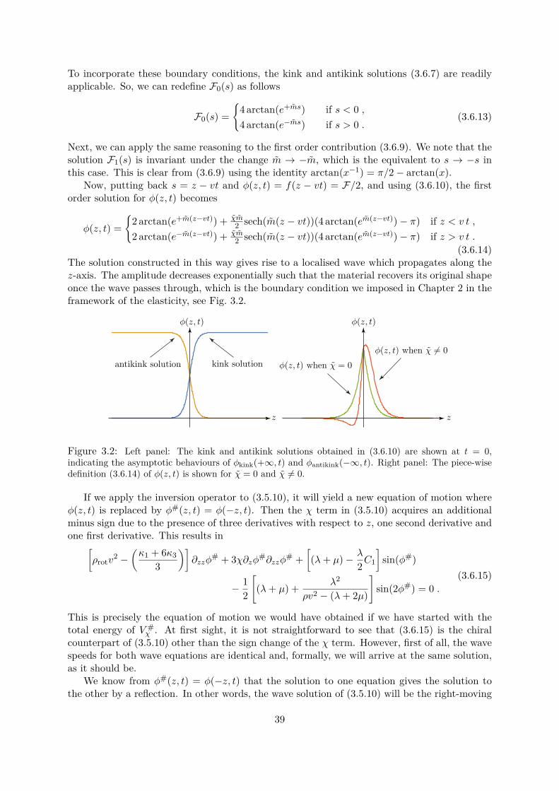
To incorporate these boundary conditions, the kink and antikink solutions (3.6.7) are readilyapplicable. So, we can redefine F0(s) as follows
F0(s) =
4 arctan(e+ms) if s < 0 ,4 arctan(e−ms) if s > 0 .
(3.6.13)
Next, we can apply the same reasoning to the first order contribution (3.6.9). We note that thesolution F1(s) is invariant under the change m → −m, which is the equivalent to s → −s inthis case. This is clear from (3.6.9) using the identity arctan(x−1) = π/2 − arctan(x).
Now, putting back s = z − vt and ϕ(z, t) = f(z − vt) = F/2, and using (3.6.10), the firstorder solution for ϕ(z, t) becomes
ϕ(z, t) =
2 arctan(e+m(z−vt)) + χm2 sech(m(z − vt))(4 arctan(em(z−vt)) − π) if z < v t ,
2 arctan(e−m(z−vt)) + χm2 sech(m(z − vt))(4 arctan(em(z−vt)) − π) if z > v t .
(3.6.14)The solution constructed in this way gives rise to a localised wave which propagates along thez-axis. The amplitude decreases exponentially such that the material recovers its original shapeonce the wave passes through, which is the boundary condition we imposed in Chapter 2 in theframework of the elasticity, see Fig. 3.2.
Figure 3.2: Left panel: The kink and antikink solutions obtained in (3.6.10) are shown at t = 0,indicating the asymptotic behaviours of ϕkink(+∞, t) and ϕantikink(−∞, t). Right panel: The piece-wisedefinition (3.6.14) of ϕ(z, t) is shown for χ = 0 and χ = 0.
If we apply the inversion operator to (3.5.10), it will yield a new equation of motion whereϕ(z, t) is replaced by ϕ#(z, t) = ϕ(−z, t). Then the χ term in (3.5.10) acquires an additionalminus sign due to the presence of three derivatives with respect to z, one second derivative andone first derivative. This results in[
ρrotv2 −
(κ1 + 6κ3
3
)]∂zzϕ
# + 3χ∂zϕ#∂zzϕ
# +[(λ+ µ) − λ
2C1
]sin(ϕ#)
− 12
[(λ+ µ) + λ2
ρv2 − (λ+ 2µ)
]sin(2ϕ#) = 0 .
(3.6.15)
This is precisely the equation of motion we would have obtained if we have started with thetotal energy of V #
χ . At first sight, it is not straightforward to see that (3.6.15) is the chiralcounterpart of (3.5.10) other than the sign change of the χ term. However, first of all, the wavespeeds for both wave equations are identical and, formally, we will arrive at the same solution,as it should be.
We know from ϕ#(z, t) = ϕ(−z, t) that the solution to one equation gives the solution tothe other by a reflection. In other words, the wave solution of (3.5.10) will be the right-moving
39
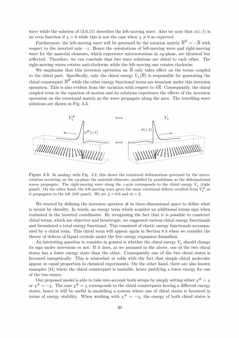
wave while the solution of (3.6.15) describes the left-moving wave. Also we note that ϕ(z, t) isan even function if χ = 0 while this is not the case when χ = 0 as expected.
Furthermore, the left-moving wave will be governed by the rotation matrix R# = −R withrespect to the inverted axis −z. Hence the orientations of left-moving wave and right-movingwave for the material elements, which experience microrotations in xy-plane, are identical butreflected. Therefore, we can conclude that two wave solutions are chiral to each other. Theright-moving waves rotates anti-clockwise while the left-moving one rotates clockwise.
We emphasise that this inversion operation on R only takes effect on the terms coupledto the chiral part. Specifically, only the chiral energy Vχ(R) is responsible for generating thechiral counterpart R# while the other energy functional terms are invariant under this inversionoperation. This is also evident from the variation with respect to δR. Consequently, the chiralcoupled term in the equation of motion and its solutions experience the effects of the inversionoperation on the rotational matrix as the wave propagate along the axes. The travelling wavesolutions are shown in Fig. 3.3.
V #χ ⇐⇒ Vχ
⇐⇒
Figure 3.3: In analogy with Fig. 2.2, this shows the rotational deformations governed by the micro-rotation occurring on the xy-plane the material elements, modelled by pendulums as the deformationalwaves propagate. The right-moving wave along the z-axis corresponds to the chiral energy Vχ (rightpanel). On the other hand, the left-moving wave gives the same rotational defects resulted from V #
χ asit propagates to the left (left panel). We set χ = 0.6 and m = 2.
We started by defining the inversion operator # in three-dimensional space to define whatis meant by chirality. In words, an energy term which acquires an additional minus sign whenevaluated in the inverted coordinates. By recognising the fact that it is possible to constructchiral terms, which are objective and hemitropic, we suggested various chiral energy functionalsand formulated a total energy functional. This consisted of elastic energy functionals accompa-nied by a chiral term. This chiral term will appear again in Section 8.4 when we consider thetheory of defects of liquid crystals under the free energy expansion formalism.
An interesting question to consider in general is whether the chiral energy Vχ should changeits sign under inversions or not. If it does, as we assumed in the above, one of the two chiralstates has a lower energy state than the other. Consequently one of the two chiral states isfavoured energetically. This is somewhat at odds with the fact that simple chiral moleculesappear in equal proportion in chemical experiments. On the other hand, there are also knownexamples [41] where the chiral counterpart is unstable, hence justifying a lower energy for oneof the two states.
Our proposed model is able to take into account both setups by simply setting either χ# = χor χ# = −χ. The case χ# = χ corresponds to the chiral counterparts having a different energystates, hence it will be useful in modelling a system where one of chiral states is favoured interms of energy stability. When working with χ# = −χ, the energy of both chiral states is
40
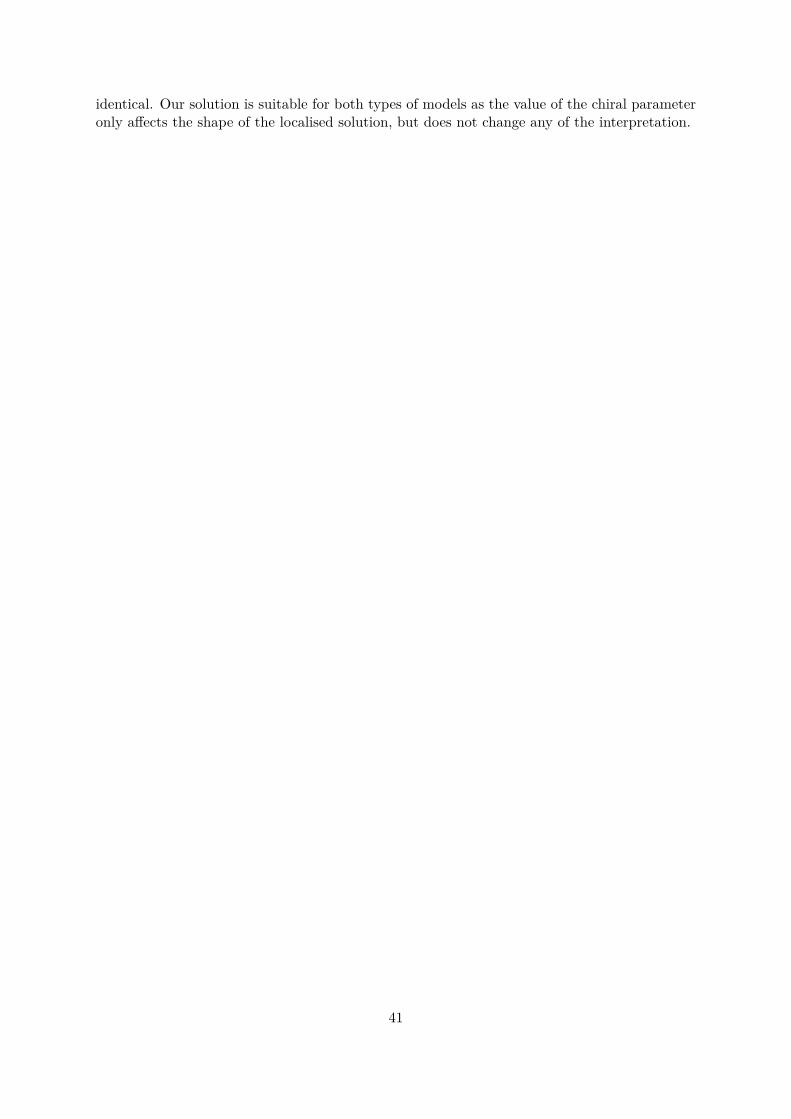
identical. Our solution is suitable for both types of models as the value of the chiral parameteronly affects the shape of the localised solution, but does not change any of the interpretation.
41

42
Part II
Defects in Riemann-Cartanmanifolds
43

Chapter 4
Background and motivation
4.1 Differential geometry and elasticity
In continuum physics, there are two distinct measures of defects, called disclination and dislo-cation. In this Chaper, we will see that these measures are related to curvature and torsion,respectively. These defect measures can be detected due to the broken symmetries, for exam-ple, in Bravais lattices, the idealised approximation of crystalline. When defects are detected,these can be explained by the broken rotational symmetries caused by the disclination, and thebroken translational symmetries caused by the dislocation [66–69].
In general relativity, the notion of curvature has been the main ingredient in describingdeformed spacetime, and the notion of torsion is largely omitted. Nonetheless, in developingthe theory for generalised local symmetry under the Poincaré group, the theory similar to thoseof Yang-Mills theory [70] in the curved spacetime, the notion of torsion has essentially becomeevident in completing the theory with the spinning particles coupled to torsion [71–75] underthe minimal prescription by promoting ordinary partial derivatives to covariant derivatives withappearances of new local gauge fields. Hence, the needs for the non-Riemann manifold arisesnaturally which can contain the Cartan’s torsion tensor.
Riemann-Cartan manifolds contain both curvature and torsion, and provide a suitable back-ground when one brings concepts of curvature and torsion to a given manifold at the same time,using the method of differential geometry in describing the intrinsic nature of defects and itsclassifications. Pioneering works using this mathematical framework were explored in [66,76–79].Inspired from similarities and its applicabilities, links between the theories of the continuumphysics and the Einstein-Cartan theory in describing the defects were made in [80–84]. It isworth noting that these geometrical considerations are commonly used in the Einstein-Cartantheory [74,85,86], teleparallel gravity [87], gauge theories of gravity [88–90] and the condensedmatter system [91–93]. In a microscopic point of view, microrotations and torsion were exploredin [21–23,82,94]. Recent developments in incorporating the elasticity theory and spinning par-ticles using the tetrad formalism can be found in [95,96].
Since the Riemann curvature tensor satisfies various geometrical identities such as Bianchi’sidentities, it is natural to expect that these identities also play a role in continuum mechanics,if one considers the possibility that the Riemann curvature tensor can contain both measuresof pure curvature originated from the metric tensor and torsion which can arise independentlyof the metric field. In particular, we will see that the vanishing Riemann curvature and itsrelated measures imply the theory is in the regime of elasticity, and a set of partial differentialequations may lead to an integrability condition which is commonly called the compatibilitycondition in some cases.
This will be our starting point in connecting the theories of defects in continuum physics
45
to those of the gravitational theory via the Riemann-Cartan geometry to see how torsion andcurvature can be conceived in both settings. For example, in [97], the notion of metric elasticityin the Riemann manifold is introduced, hence it is essentially required to bring the notionof force in the formalism which is one of distinct features from the conventional theory ofgravitation [85].
It is well known that the vanishing Riemann curvature tensor in the deformed body yieldsthe compatibility conditions equivalent to the Saint-Venant compatibility conditions [98–103]in the classical elasticity theory, which are otherwise derived by considering higher order partialderivatives, that have to necessarily commute. After revisiting these basic results in the classicaltheory of continuum, we will show that one of compatibility conditions known as the Vallée’scompatibility condition, is in fact equivalent to the vanishing of the three-dimensional Einsteintensor using tools of differential geometry and we will develop its further implications. In PartII, we will follow closely the results obtained in [104].
4.2 Compatibility conditionsCompatibility conditions in continuum mechanics form a set of partial differential equationswhich are not completely independent of each other. They may impose certain conditions amongunknown number of functions which are often derived by applying higher-order mixed partialderivatives to given system of equations. They are closely related to integrability conditions.
In 1992 Vallée [105] showed that the standard Saint-Venant compatibility condition of linearelasticity, known since the mid-19th century, can be written in the convenient form
Curl Λ + Cof Λ = 0 , (4.2.1)
where the operators Curl and Cof in (4.2.1), for 3 × 3 matrices, are defined by
(Curl Λ)ij = ϵjmn∂mΛin , and (Cof Λ)ij = 12ϵimsϵjntΛmnΛst , (4.2.2)
and ϵijk is the totally antisymmetric Levi-Civita symbol for i, j, k = 1, 2, 3. The 3 × 3 matrix Λis given by
Λ = 1detU
[U(CurlU)TU − 1
2tr[(CurlU)TU
]U
]. (4.2.3)
This formulation is based on Riemannian geometry where the metric tensor is written as gµν =Ua
µUbνδab. Here U is the right stretch tensor of the polar decomposition of the deformation
gradient tensor F = RU of (1.2.6), and R is an orthogonal matrix which is the polar part.Condition (4.2.1) is derived by finding the integrability condition of the system for the right
Cauchy-Green deformation tensor C defined in (1.2.35),
C = (∇Θ)T (∇Θ) . (4.2.4)
The deformation of the continuum is expressed by a diffeomorphism Θ : M → R3 in the classicaltheory, such that x = X +u with u being the displacement vector. Hence, the tensor C assumesthe role of a metric tensor in the given smooth manifold M . Later [106], the existence of suchan immersion Θ is proved which maps an open subset of R3 into R3 in which the metric tensorfield defined by C with U in the polar decomposition ∇Θ = RU . The expression (4.2.1) willbe shown to be equivalent to the vanishing of the Riemann curvature tensor in this settingand the zero curvature characterises the differential equation (4.2.4) to be integrable. For asmall displacement field u, the notion of zero curvature reduced to the classical Saint-Venantintegrability conditions.
46
Much earlier, in 1953 Nye [34] showed that there exists a curvature related rank-two tensorΓ of the form
Γ = 12tr
(RT CurlR
)1 − (RT CurlR)T , (4.2.5)
satisfying the identical form of compatibility condition
Curl Γ + Cof Γ = 0 . (4.2.6)
The object Γ is often called Nye’s tensor, and is written in terms of the dislocation densitytensor K = RT CurlR we used in constructing the energy functional Vcurvature and Vχ in Part I,for example (3.2.14) and (3.3.8). We note that the dislocation density tensor here only dependson the orthogonal matrix R.
We would like to show that these two compatibility conditions (4.2.2) and (4.2.6), seeminglyarose from different and incomparable settings, are in fact special cases of a much broadercompatibility condition which can be formulated in Riemann-Cartan geometry.
47

48
Chapter 5
Deformational measures inRiemann-Cartan manifold
We introduce frame basis and co-frame basis, also called tangent and co-tangent basis respec-tively, together with its polar decompositions. Then we define various quantities including ageneral affine connection, a spin connection, and torsion formally. We decompose these tensorsinto two parts, one which is torsion-free and one that contains torsion. The Riemann tensor willbe expressed in various ways using above mentioned tensors. We then introduce the Einsteintensor in terms of Riemann curvature tensor in three dimensions.
5.1 Frame fields and non-frame fieldsLet us begin with a three-dimensional Riemannian manifold M with coordinates x, and let usintroduce a set of bases for the tangent space and co-vectors (or 1-forms) for the co-tangentspace, respectively, at some point x ∈ M
Eµb (x) and ea
µ(x) (5.1.1)
where the Latin indices a, b, · · · = 1, 2, 3 are tangent space indices, and Greek letters µ, ν, · · · =1, 2, 3 denote coordinate indices. This basis is often called a (co-)tetrad field. For the framefield, we define the tangent basis
Ea = Eµa
∂
∂xµ, (5.1.2)
where Eµa is an element of 3 × 3 real general linear group GL(3; R). So we can say that Ea is
obtained by the transformation of the frame fields ∂/∂xµ by some element Eµa . Similarly, we
define the co-frame field (or co-tangent field), the dual fields of frame field,
ea = eaµdx
µ , (5.1.3)
where eaµ is also an element of GL(3; R). These satisfy orthogonal relations
eaµE
νa = δν
µ and eaµE
µb = δa
b . (5.1.4)
Here δνµ and δa
b are the Kronecker deltas in their respective spaces. We emphasise that for agiven manifold, we can find these tangent bases locally so that we can relate different sets oftangent bases in different points by simple transformations defined by an element GL(3; R).
However, it is impossible to find a single frame field which is nowhere vanishing globally,unless the manifold is completely parallelisable. For example, the hairy ball theorem [107]
49
illustrates that we cannot comb the hair on a 2-sphere S2, embedded in three dimensions,smoothly everywhere. Hence this justifies the use of the locally defined diffeomorphism as theimmersion of Θ : M → R3 used in (4.2.4).
In the framework of tetrad formalism, the metric tensor emerges as a secondary quantitydefined in terms of tetrad fields. We have
gµν(x) = eaµ(x)eb
ν(x)δab , (5.1.5)
where δab is the globally flat Euclidean metric with the signature (+1,+1,+1) in three dimen-sions. And it is easy to see that its inverse is gµν , defined by
gµν(x) = Eµa (x)Eν
b (x)δab .
Using these, we can raise and lower indices of the (co-)tangent frame objects by applying gµν ,δab, and its corresponding inverses. In Riemannian geometry, the metric (5.1.5) gives rise to aninvariant length element under a general diffeomorphism and a tangent space transformation,
(ds)2 = gµνdxµdxν = ea
µebνδabdx
µdxν = eaebδab , (5.1.6)
and similarly for the Eµa field.
This means we can use the co-tangent basis eaµ to describe the local deformation given by the
metric tensor gµν from the flat space δab written in the coordinate basis. As a result, the metrictensor gµν is obtained from the flat Euclidean metric δab by a set of deformational informations,encoded in ea
µ(x) ∈ GL(3; R) at each point x ∈ M . Since any deformation can be regardedas a combination of rotation, shear and compression, the common terms in (micro)continuumphysics, we can apply the polar decomposition to ea
µ as we did in Part I,
eaµ(x) = Ra
b(x)U bµ(x) , (5.1.7)
where Rab is an orthogonal matrix (a pure tangent space object with Latin indices) while
the field U bµ is a symmetric and positive-definite matrix. Whenever we need to distinguish
the microdeformations from the macrodeformations, we will put a bar over the correspondingtensor. When this decomposition is applied to (5.1.5) one arrives at
gµν = RacRadU
cµU
dν = δcdU
cµU
dν , (5.1.8)
which shows that the metric is completely independent of Rab and only depends on U b
µ. This isa well-known result in differential geometry, namely, the metric field is independent of tangentspace rotations. The polar decomposition for the inverse frame can be similarly written by
Eµa = R b
a Uµb , (5.1.9)
so that Uµb is the inverse of Ua
µ , both of which are positive-definite and symmetric. Consequently,the co-tangent basis given by a specific metric tensor (5.1.5) is not uniquely determined. Thiscan be seen by counting the number of required independent parameters in the expression ofthe symmetric metric tensor (5.1.5). Hence, the additional number of degrees of freedom on thetetrad fields implies that any two (co-)tetrads ea
µ and eaµ will yield the same metric provided
they are related by a rotation
eaµ = Qa
bebµ , Qa
b ∈ SO(3) . (5.1.10)
A metric compatible covariant derivative is introduced in differential geometry through thecondition
∇λgµν = 0 . (5.1.11)
50

This introduces the Christoffel symbol components Γλµν as the general affine connection. From
(5.1.5), it is natural to assume that in the tetrad formalism,
∇µeaν = 0 . (5.1.12)
This, in turn, will uniquely determine the spin connection coefficients ω aµ b(x),
0 = ∇µeaν = ∂µe
aν − Γλ
µνeaλ + ω a
µ bebν , (5.1.13)
where Γµλν is a general affine connection, and the lower indices in this connection are not nec-
essarily symmetric. Using the orthogonality (5.1.4), we can rewrite (5.1.13) by
ω aµ b = ea
λΓλµνE
νb + ea
ν∂µEνb . (5.1.14)
Note that the spin connection is invariant under global rotations but not under local rotations.And the derivative terms will pick up additional terms, this is of course expected when workingwith connections.
The covariant derivative for a general vector V µ in coordinate space is defined by
∇λVµ = ∂νV
µ + ΓµλνV
ν . (5.1.15)
Being equipped with the frame (and co-frame) field, we might introduce a quantity,
V a = eaµV
µ (5.1.16)
which denotes the tangent space components of a general vector V µ. We can see that the vectorV µ is rotated by the tetrad ea
µ to become V a in the tangent field. It is easy to see that its inverserelation is simply V µ = Eµ
aVa. Naturally, the covariant derivative of V a can be described using
the spin connection, in view of (5.1.15). This gives
∇µVa = ∂µV
a + ω aµ bV
b , (5.1.17)
and can be extended to higher-rank objects in the same way.For completeness, we state the inverse of (5.1.14), so that the general affine connection is
expressed in terms of the spin connection
Γλµν = Eλ
aωa
µ bebν + Eλ
a∂µeaν . (5.1.18)
Equations (5.1.14) and (5.1.18) together with the (co-)frame allow us to express geometricalidentities in either the tangent space or the coordinate space.
In general, unlike the coordinate bases ∂/∂xµ, the non-coordinate bases Ea = Eµa∂µ do
not commute, and one introduces the object of anholonomity as follows. Let u be a smoothdifferentiable function, then a direct and straightforward calculation gives
[Ea, Eb]u = EµaE
νb (∂νe
cµ − ∂µe
cν)Ecu . (5.1.19)
This must be valid for the arbitrary u, so we can write
[Ea, Eb] = f cabEc , (5.1.20)
where the f cab are the structure constants, which are given by
f cab = Eµ
aEνb (∂νe
cµ − ∂µe
cν) . (5.1.21)
51
5.2 Torsion and curvature
Given a general affine connection, the torsion tensor is defined by
T λµν = Γλ
µν − Γλνµ , (5.2.1)
which is the antisymmetric part of the connection.Throughout this paper, we will use the decomposition of the various tensor quantities into
a torsion-free part and a separate torsion part. These correspond to the quantities in Riemannspace and the quantities in non-Riemann space. Also we will use the notation “ ” specificallyindicating the torsion-free quantities, or equivalently the quantities written in terms of themetric compatible connection which is generally referred to as the Christoffel symbol.
The main reason for this process is that by applying these decompositions to various defor-mational measures both in Riemann and non-Riemann space, we might hope to see the relationsbetween the compatibility conditions, introduced in Section 4.2, originated from the distinctspace connected by some additional fields.
First we decompose the general affine connection
Γρνσ =
Γρ
νσ +Kρνσ , (5.2.2)
which introduces the contortion tensor Kρνσ. Using the definition of torsion (5.2.1), we im-
mediately haveT λ
µν = Kλµν −Kλ
νµ , (5.2.3)
which one can also solve for the contortion tensor. This yields
Kλµν = 1
2(T λ
µν + T λν µ − T λ
µν
), (5.2.4)
which in turn implies the antisymmetric property Kλµν = −K λ
νµ .The Riemann curvature tensor is defined by
Rρσµν = ∂µΓρ
νσ − ∂νΓρµσ + Γρ
µλΓλνσ − Γρ
νλΓλµσ (5.2.5)
where Γρνσ are the general affine connections.
Using the frame fields, we can introduce those tensors with mixed components (indicesfor coordinate space and tangent space), which will turn out to be useful for our subsequentdiscussion. We define a GL(3; R)-rotated torsion tensor by
T aµν = ea
λTλµν , (5.2.6)
Using (5.1.18), or the expression ∇µeaν − ∇νe
aµ = 0, we can write the torsion tensor in the
following equivalent way,
T aµν = ∂µe
aν − ∂νe
aµ + ω a
µ bebν − ω a
ν bebµ . (5.2.7)
Similarly, we can rewrite the Riemann tensor with mixed indices
Rabµν = ea
ρRρσµνE
σb , (5.2.8)
which allow us to write the Riemann tensor entirely in terms of the spin connections
Rabµν = ∂µω
aν b − ∂νω
aµ b + ω a
µ eωe
ν b − ω aν eω
eµ b . (5.2.9)
52
In addition to the antisymmetry in the last two indices in the Riemann tensor, this satisfies
Rabµν = −Rbaµν . (5.2.10)
In this way, we can recognise the torsion and Riemann curvature tensors of (5.2.7) and(5.2.9) are two-forms in the language of differential geometry, written conveniently
T a = dea + ωab ∧ eb , (5.2.11a)
Rab = dωa
b + ωae ∧ ωe
b . (5.2.11b)
These are known as the Cartan’s structure equations.As a consequence of the decomposition (5.2.2), we apply the same concept to the spin
connection to write its decomposition
ω aµ b =
ω aµ b +Ka
µb , (5.2.12)
where we used Kaµb = ea
νKνµσE
σb . Inserting the relation (5.2.12) into (5.2.9) gives the decom-
position of the Riemann tensor,
Rρσµν =
Rρ
σµν +[ ∇µK
ρνσ −
∇νK
ρµσ +Kρ
µλKλνσ −Kρ
νλKλµσ
], (5.2.13)
where the Riemann tensorRρ
σµν is computed using the metric compatible connectionΓρ
µν
entirely.We note that, for a general vector V ρ, in the coordinate basis, the covariant derivative can
be rewritten using (5.2.2) such that
∇µVρ =
∇µV
ρ +KρµνV
ν . (5.2.14)
This relates the general covariant derivative ∇µ and the torsion-free, metric compatible covariantderivative
∇µ used in (5.2.13). In addition to (5.2.2) and (5.2.12), we can regard the contortion
tensor on the right-hand side as the connection between these two distinct covariant derivatives.
5.3 Einstein tensor in three-dimensional spaceWe define a rank-two quantity based on the spin connection by
Ωcµ = −12ϵabcω
abµ , (5.3.1)
which is equivalent toω ab
µ = −ϵabcΩcµ . (5.3.2)
This is somewhat similar to extracting information of an axial field from a generator of arotational matrix. A three-dimensional rotational matrix can be written in the exponentialrepresentation R = eA with its antisymmetric generator Aij = θaij and the rotation of an angleθ about the axis ni = −1
2ϵijkajk.We note that this construction is only valid in three dimensions to arrive at a rank-two
object in (5.3.1). In the following, it will turn out that Ωcµ plays a crucial role in establishingour compatibility conditions. The same approach was applied to the torsion tensor in [21] wherethe setting was also R3.
We substitute (5.3.2) into the Riemann tensor (5.2.9), and find
Rabµν = ϵsa
b (−∂µΩsν + ∂νΩsµ) + ϵsaeϵ
teb (ΩsµΩtν − ΩsνΩtµ) . (5.3.3)
53

Next, we define another rank-two tensor, constructed from the Riemann tensor,
Gσc = −14ϵ
abcRabµνϵµνσ , (5.3.4)
in which the Riemann curvature tensor on the left-hand side is antisymmetric in the first andsecond pairs of indices. Let us emphasise again that this construction is only possible in threedimensions, otherwise we would need to introduce a different rank in the Levi-Civita symbol.
Inserting (5.3.3) into (5.3.4), using the facts ϵabcϵsab = 2δcs and ϵsaeϵ
abcϵteb = −ϵtcs, we obtain
Gσc = ϵµνσ∂µΩcν + 1
2ϵcstϵσµνΩsµΩtν , (5.3.5)
which can be written in the convenient form
Gσc = (Curl Ω)cσ + (Cof Ω)cσ . (5.3.6)
The quantity Gσc is, in fact, the Einstein tensor in three-dimensional space. This can be shownusing (5.3.5) and (5.2.8) explicitly to obtain the familiar expression for the Einstein tensor,
Gτλ = Rτλ − 12δτλR . (5.3.7)
Here Rτλ is the Ricci tensor defined by Rτλ = Rστσλ, and the trace of Ricci tensor is the Ricci
scalar R. It is well known that in three dimensions, the Riemann tensor, the Ricci tensor, andthe Einstein tensor have the same number of independent components, namely nine, providedtorsion is included. Therefore, unlike the conventional theory of gravitation, the symmetricRicci tensor and Einstein tensor are not assumed. One can readily verify that following threerelations are equivalent to each other.
Rabµν = 0 ⇐⇒ Rτλ = 0 ⇐⇒ Gτλ = 0 . (5.3.8)
In other words, the vanishing curvature means vanishing Einstein tensor in three dimensions.
54
Chapter 6
Compatibility conditions
We are in position to use the tools of differential geometry, various deformational measures, andits decompositions. We will derive compatibility conditions in various physical settings usinga universal process. Firstly, Vallée’s result will be re-derived, followed by Nye’s condition. Wecarefully explain the connection between these two compatibility conditions, all explanationsare originated from the vanishing Einstein tensor. We will show an extension of this result tothe microcontinuum theories, and lastly we will derive a general compatibility condition, whichis applicable to the case of nonzero curvature.
6.1 Vallée’s classical resultWe consider the torsion-free spin connection
Ωcµ = −1
2ϵabcω ab
µ with the metric tensor (5.1.5).The affine connection in torsion-free space is conventionally expressed by the metric compatibleLevi-Civita connection which enters into the decomposition of (5.2.2),
Γλ
µν = 12g
λσ (∂νgσµ + ∂µgσν − ∂σgµν) . (6.1.1)
The torsion-free spin connection in terms of the Levi-Civita connection is simplyω a
µ b = eaλ
Γλ
µνEνb + ea
ν∂µEνb
= 12e
aλg
λτ (∂νgτµ + ∂µgτν − ∂τgµν)Eνb + ea
ν∂µEνb ,
where we used (5.1.14). Inserting the explicit expression for the metric tensor (5.1.5) will give,after a lengthy but straightforward calculation,
ω a
µ b = 12E
σb
(∂σe
aµ − ∂µe
aσ
)− 1
2δadδfbE
σd
(∂σe
fµ − ∂µe
fσ
)+ 1
2δadgµσ (∂dE
σb − ∂bE
σd ) (6.1.2)
in which we defined ∂a = Eσa ∂σ. This expression for the torsion-free spin connection is particu-
larly useful in such a way that we can write the spin connection in terms of polar decompositionof co-frame field basis ea
µ = RabU
bµ to write
ω abµ entirely in terms of Ra
b and U bµ, and its deriva-
tives. By doing so, we can split deformational measures in terms of the metric-dependent part,which only sees the stretches U b
µ, and the metric-independent part depending only on the rota-tions Ra
b. The resulting expressions will be further simplified if we consider the cases Rab = δa
b
and U bµ = δb
µ separately, to see whether these will lead to the desired compatibility conditions.First, when Ra
b = δab , after multiplying ϵabc to both sides of (6.1.2), we have
ϵabcω ab
µ = ϵabcϵσµνUaν(CurlU)bσ − 1
2ϵabcϵστρUaρU bσ(CurlU) τ
f Ufµ . (6.1.3)
55
We can extract the determinant of U from the first and the second term in the right-hand sideof this,
ϵabcϵσµνUaν(CurlU)bσ = 6
detU[U(CurlU)TU
]cµ,
ϵabcϵστρUaρU bσ(CurlU) τ
f Ufµ = 6
detU Ucµtr[(CurlU)TU
].
(6.1.4)
Therefore, we find
Ωcµ = −3 1
detU
[U(CurlU)TU − 1
2tr[(CurlU)TU
]U
]cµ. (6.1.5)
The vanishing Riemann tensor in three-dimensional space ensures the vanishing Ricci tensor,hence the vanishing Einstein tensor
Gµc = 0, as stated in (5.3.8). This leads to the compatibility
condition in the torsion-free space of vanishing Riemann curvature, with the help of (5.3.6),
CurlΩ + Cof
Ω = 0 . (6.1.6)
Of course, we can rescale −13
Ω = ΛU to match the Vallée’s result [105] exactly
ΛU = 1detU
[U(CurlU)TU − 1
2tr[(CurlU)TU
]U
], (6.1.7)
which readsCurl ΛU + Cof ΛU = 0 . (6.1.8)
This result indicates that, as long as ΛU satisfies the compatibility condition (6.1.8), thedeformation can be compatible to that of trivial case Ua
µ = δaµ regardless of the details of the
stretch Uaµ , where the deformational description of Ua
µ itself undergoes the transformation by themetric tensor gµν . This implicitly suggests that the compatibility condition (6.1.8) is invariantunder the diffeomorphism in a given manifold. Therefore, we can conclude that the larger classof solution space for the expression (4.2.4), which depends on Ua
µ , can be classified as the distinctset of equivalent classes.
This means that the elastic deformation is nothing but the diffeomorphism described by ametric tensor with an associated metric compatible connection
Γλ
µν as the fundamental measureof the deformation. Then, the prescription of elastic deformations requires vanishing curva-ture and torsion, hence the compatibility conditions (6.1.8) in the absence of the torsion orequivalently Ra
b = δab in this case, is precisely the statement of the elasticity.
We should also note the results of Edelen [108] where compatibility conditions were derivedusing Poincaré’s lemma. This resulted in the vanishing Riemann curvature two-form, Eq. (3.3)in [108] while assuming the metric compatible connection, Eq. (3.4) in [108]. These conditionsexplicitly contained torsion due to the affine connection being non-trivial but curvature free.
6.2 Nye’s tensor and its compatibility conditionNext, we set U b
µ = δbµ but assume a non-trivial rotation matrix Ra
b. This will give the expressionscompletely independent of metric tensor. And we might hope to see how the rotational fieldscontribute to the deformational expressions. To do so, we notice that the setting is alreadygiven in (6.1.2) and we put the non-trivial rotations Ra
b but the trivial stretches Uaµ = δa
µ,hence we are still in the regime of zero curvature. This space is often referred as Weitzenböckspace especially in the field of Teleparallel Gravity.
56
The calculation is identical if we replace the stretch parts by the rotation parts in deriving(6.1.8), starting from the torsion-free spin connection (6.1.2) after applying the decompositionea
µ = RabU
bµ. The final compatibility condition is then
Curl ΛR + Cof ΛR = 0 , (6.2.1)
where the quantity ΛR is given by
ΛR = R(CurlR)TR− 12tr
[(CurlR)TR
]R . (6.2.2)
This confirms the replacing U cµ with Ra
b in (6.1.7) and using detRab = +1.
It turns out that the quantity ΛR is (up to a minus sign) Nye’s tensor Γ which is knownto satisfy the compatibility condition (6.2.1). This is quite a remarkable result which followsimmediately from our geometrical approach to the problem.
• We emphasise that the metric tensor is independent of the rotations which implies thatU c
µ = δcµ yields a vanishing (torsion-free) Levi-Civita connection
Γλ
µν . Consequently theLevi-Civita part of the curvature tensor vanishes identically,
Rρ
σµν = 0.
• The compatibility condition simply ensures that the micropolar deformations governedby Ra
b do not induce curvature in the deformed body. We will see the mathematicaljustification of this fact shortly, but most importantly, nonzero torsion do not contributethe Riemann curvature tensor (hence the Einstein tensor), and we obtain the compatibilitycondition by simply replacing Ua
µ by Rab from the previously obtained result.
Now, one of most significant consequences of the decomposition (5.2.2) we started with isthe following. In the space where
Γλ
µν = 0, or equivalently U cµ = δc
µ but with non-vanishingtorsion, the general affine connection reduces to the contortion. Moreover, in the manifoldof vanishing curvature, the Cartan’s structure equation (5.2.11b) of the Riemann curvaturetwo-form becomes
dω = −ω ∧ ω .
It is known that the spin connection depends purely on the symmetry group of an inertialframe [87] (e.g the Lorentz transformation, or the Galilean transformation in the non-relativisticlimit). Then one can choose such a frame so that dω = 0. In other words, the curvature two-form now induces an integrable expression for the spin connection. Further, with the use ofFrobenius theorem as introduced in [109], the spin connection becomes trivial, and one can putω a
µ b = 0 in (5.1.18) without loss of generality. Then we have
Γλµν = (R b
a δλb )∂µ(Ra
cδcν) = δλ
b δcν(R b
a ∂µRac) = δλ
b δcνδ
dµ(R b
a ∂dRac) . (6.2.3)
The final term in the brackets is recognised to be the second Cosserat tensor when written inindex free notation RT GradR, see for instance [110].
In the following, we will briefly discuss how the compatibility condition for Nye’s tensor canalso be derived directly without referring to the general result we will see in Section 6.4. Inorder to have completely vanishing curvature tensor (5.2.13) with U c
µ = δcµ, we note another
observation in addition to above mentioned consequences. That is, we can replace∇µ with ∂µ
in (5.2.13). Under these circumstances, the Riemann curvature tensor (2.3.7) reduces to
Rρσµν = ∂µK
ρνσ − ∂νK
ρµσ +Kρ
µλKλνσ −Kρ
νλKλµσ . (6.2.4)
57
Now, we would like to formally define a rank-two tensor Kλσ which is the dislocationdensity tensor [21, 31, 111], by contracting the contortion tensor with ϵσµν , in a similar waywe did in (5.3.1),
Kλσ = ϵσµνKλµν . (6.2.5)
This also gives a relation between the torsion tensor and the dislocation density tensor by
Kλσϵσµν = T λαβ . (6.2.6)
For our explicit choice of the contortion tensor in (6.2.3), we can write the dislocation densitytensor by
Kλσ = ϵ µνσ δλbR
ba ∂µR
acδ
cν =
(RT CurlR
)λσ
. (6.2.7)
This is nothing but the dislocation density tensor (2.1.5), we used throughout Part I, as appearedin the formulation of the energy functionals (2.1.2) (we dropped the bar here).
For Nye’s tensor, we contract the first and third index of the contortion tensor
Γλν = −12ϵ
ρσλ Kρνσ . (6.2.8)
In turn, the relation between Nye’s tensor and the contortion tensor becomes Γλνϵλ
µρ = −Kµνρ.From this, the contortions can be substituted into (6.2.4) to write the Riemann curvature interms of Nye’s tensor entirely. This immediately yields
Curl Γ + Cof Γ = 0 . (6.2.9)
This is our second compatibility condition written in terms of Nye’s tensor, for the vanishingcurvature and nonzero torsion tensor.
We note that combining the definitions of (6.2.5) and (6.2.8) together leads to the usualexpression of Nye’s tensor, originally introduced in [34]
Γλν = 12tr
(RT CurlR
)δλν − (RT CurlR)T
λν . (6.2.10)
Inversely, we can express the dislocation density tensor in terms of Nye’s tensor
Kλσ = Γµµδλσ − (ΓT )λσ . (6.2.11)
One might get an impression from (6.2.4) that non-vanishing curvature might be inducedby the non-vanishing contortion or torsion. However, this is not the case. As indicated inSection 10.3, the contortion tensor is of Maurer-Cartan form K = RTdR which satisfies theMaurer-Cartan equation
dK = −K ∧ K , (6.2.12)which is equivalent to the expression of the vanishing Riemann curvature tensor entirely in theform of (6.2.4).
6.3 Eringen’s compatibility conditionsNow we would like to see how we can apply the results we obtained so far to the theoryof microcontinuum, especially to the micropolar case. We will follow the notations used byEringen in [15]. Strain measures introduced in (1.2.37) and (1.2.38) are
CKL = ∂xk
∂XKXLk CKL = χkKχkL = CLK
ΓKLM = XKk∂χkL
∂XMΓKL = 1
2ϵKMN ΓNML
(6.3.1)
58
with the directors ΞK and ξk in material coordinate XK , and spatial coordinate xk, respectively.Now we recognise that the symmetric microdeformation tensor CKL is analogous to the metrictensor in the form of (5.1.5).
In case of micropolar continua, it is easy to see the existence of the compatibility conditionsby counting and comparing the total number of independent variables and the number of par-tial differential equations in the definitions of (6.3.1), for a given dimension. Specifically, withthe possible symmetric property in mind, we note that the variables xk, χkX are not inde-pendent, but these are related to each other. So, the simplest form of integrability conditionsfor these variables can be constructed from first-order partial differential equations ∂Kxk = 0and ∂LχkK = 0, where ∂K = ∂/∂XK . And the necessary and sufficient condition for theseintegrability conditions are
∂2xk
∂XP∂XQ= ∂2xk
∂XQ∂XPand ∂2χkK
∂XP∂XQ= ∂2χkK
∂XQ∂XP. (6.3.2)
The deformational tensors of (6.3.1) can be decomposed into rotation and stretch parts,again the polar decomposition, as we did in the tetrad bases ea
µ and Eνa . For example, after
changing indices in accordance with the current use, we can rewrite the transformations betweendirectors, χ and X, with the above mentioned deformational tensors,
χac = R
abU
bc (6.3.3a)
X ca = R
ba U
cb (6.3.3b)
Cµa = X c
a Fµ
c = Rb
a UcbR
dc U
µd (6.3.3c)
Cbc = χabχac = R
aeU
ebRadU
dc (6.3.3d)
Γklm = χak∂mχal = R
abU
bk∂m(RacU
cl ) , (6.3.3e)
in which we used bars over the the micro-deformations and used definition for the (macro)deformationgradient tensor F , with its polar decomposition into macrorotation and macrostretch.
The compatibility conditions for the micromorphic body [15] are given by
ϵKP Q (∂QCP L + CP RΓLRQ) = 0 , (6.3.4a)ϵKP Q (∂QΓLMP + ΓLRQΓRMP ) = 0 , (6.3.4b)
∂MCKL − (ΓP KMCLP + ΓP LMCKP ) = 0 . (6.3.4c)
It is evident from (6.3.3e) that the wryness tensor ΓKLM can be viewed as the contortiontensor in differential geometry, so we can make a replacement ΓP KM → KP
MK , hence thecompatibility condition (6.3.4c) now becomes
∂MCKL −KPMKCP L −KP
MLCKP = 0 . (6.3.5)
Using the decomposition (5.2.2) withΓP
MK = 0, this will further reduce to
∇MCKL = 0 . (6.3.6)
This condition is now equivalent to the assumption (5.1.11) on the metric tensor, one of ourassumptions of the geometrical approach, which is not derived from the integrability condition(6.3.2).
Next, we consider condition (6.3.4b). Using the replacement of ΓP KM → KPMK gives
∂QKL
P M − ∂PKL
QM +KLQRK
RP M −KL
P RKR
QM = 0 . (6.3.7)
59
The left-hand side of this is precisely in the form of the Riemann curvature tensor (5.2.5), hencethis condition is equivalent to RL
MQP = 0. The same result can be derived if one expands theexpression using the definitions of (6.3.1) and the conditions (6.3.2), in which the symmetry inP and Q, and antisymmetry in ϵKP Q yield the zero.
Lastly, for (6.3.4a) one writes
ϵKP Q
(∂QCP L +KL
QRCP R
)= 0 , (6.3.8)
which is known as the compatibility condition for the disclination density tensor. After somealgebraic manipulation ,(6.3.8) can be rewritten as
∇QCLP − ∇PC
LQ + TR
P QCLR = 0 , (6.3.9)
and can be seen as the definition of torsion on the manifold, equivalent to (5.2.7).For the micropolar case, by setting the the change of microvolume element (1.2.21) to the
unityj ≡ det
(∂ξk
∂ΞK
)= detχkK = 1
detXKk= 1 , (6.3.10)
i.e. χkK ∈ SO(3), the rigid microrotation, the compatibility conditions of (6.3.4) are reducedto
ϵKP Q
(∂CP L
∂XQ+ ϵMLN ΓNQCP M
)= 0 , (6.3.11a)
ϵKP Q
(∂ΓLQ
∂XP+ 1
2ϵLMN ΓMP ΓNQ
)= 0 , (6.3.11b)
whereΓKL = 1
2ϵKMN∂χkM
∂XLXNk = 1
2ϵKMN ΓNML = −12ϵKNMKN
LM (6.3.12)
which agrees with our definition for the Nye’s tensor (6.2.8). Now, in the micropolar case, weput microstretch and macrorotation to be identities in (6.3.3) so that
χac = R
ac , Cµ
c = Eµc , Cbc = δbc . (6.3.13)
Then the condition (6.3.11b) remains as the statement of vanishing Riemann curvature tensor,and the condition (6.3.6) of the micromorphic case disappears. This is because we have nowthe trivial expression CKL = δKL for the micropolar, hence the metric tensors do not see themicrorotations, as expected.
6.4 Geometrical compatibility conditions for the general caseWe considered the compatibility conditions under two settings so far, namely the implicationsof Ua
µ = δaµ and Ra
b = δab separately,
U cµ = δc
µ =⇒Γλ
µν =Ωcµ =
ω aµ b = 0 =⇒
Rρ
σµν = 0 and Rρσµν = 0 ,
Rab = δa
b =⇒ Kλν = Γλν = Kανβ = 0 =⇒ T λµν = 0 .
(6.4.1)
However, the converses of these statements are not true in general, as will be shown shortly,when deriving the general form of the compatibility conditions.
The geometrical starting point for all compatibility conditions is the Bianchi identity whichis satisfied by the curvature tensor, and is given by, see for instance [112]
∇ρRab
µν + ∇νRab
ρµ + ∇µRab
νρ = RabτνT
τµρ +Rab
τµTτρν +Rab
τρTτνµ . (6.4.2)
60
For completeness, we also state the well-known identity
Rρσµν +Rρ
µνσ +Rρνσµ = ∇σT
ρµν +∇µT
ρνσ +∇νT
ρσµ−T ρ
σλTλµν −T ρ
µλTλνσ −T ρ
νλTλσµ , (6.4.3)
for the Riemann curvature tensor which will also be required. Using Rabµν = Rλσ
µνeaλe
bσ, and
contracting twice over indices λ and ρ, and σ and ν, gives the well-known doubly contractedBianchi identity,
∇ρ
(Rρ
µ − 12δ
ρµR
)= Rλ
τTτµλ + 1
2Rλσ
τµTτλσ . (6.4.4)
The term in the first bracket on the left-hand side is the Einstein tensor, so that the mostgeneral compatibility condition can be written as
∇ρGρµ = Rρ
τTτµρ + 1
2Rρσ
τµTτρσ . (6.4.5)
Equation (6.4.5) can be seen as a compatibility or integrability condition in the following sense.One cannot choose the curvature tensor and the torsion tensor fully independently as the aboveequations need to be satisfied for a consistent geometrical approach. Hence we might expectthere is some relation between the torsion and curvature related measures.
Let us now recall (5.3.6), the Einstein tensor in terms of Ω, which is G = Curl Ω + Cof Ω.Next, we use the decomposition of the spin connection (5.2.12) into the definition of Ω of (5.3.1)to obtain
Ωcµ = −12ω
abµ ϵabc = −1
2(
ω ab
µ +Ka bµ
)ϵabc =
Ωcµ + Γcµ . (6.4.6)
When this decomposition is put into the expression of the explicit Einstein tensor, a straight-forward calculation yields,
Gλc = (Curl Ω)cλ + (Cof Ω)cλ
= Curl (Ω + Γ)cλ + Cof (
Ω + Γ)cλ
= (CurlΩ)cλ + (Curl Γ)cλ + 1
2ϵcabϵλµν
( Ωaµ + Γaµ
) ( Ωbν + Γbν
)=
(CurlΩ)cλ + (Cof
Ω)cλ
+
(Curl Γ)cλ + (Cof Γ)cλ
+ ϵcabϵλµνΩaµΓbν .
(6.4.7)
The final term is a cross-term which mixes the curvature and the torsion parts of the connection.Without this term one of the compatibility conditions would necessarily implies the other, henceit is precisely the presence of this term which gives the general condition a much richer structure.
Using (6.4.5) and (6.4.7), we are now ready to present a universal process in deriving thecomplete description of compatibility conditions encountered so far
Case I: No curvature and no torsion
Let us set Rρσµν = 0 and T λ
µν = 0 in (6.4.7). Then we must also have Kbν = Γbν = 0 by thedefinitions, and we find the compatibility condition
Gλc = (Curl
Ω)cλ + (Cof
Ω)cλ = 0 , (6.4.8)
which is Vallée’s result (6.1.6) discussed earlier.
61
Case II: No curvature and nonzero torsion
Let us set Rρσµν = 0 and T λ
µν = 0 in (6.4.7) which becomes
Gλc =
(Curl Γ)cλ + (Cof Γ)cλ
+ ϵcabϵλµνΩaµΓbν = 0 . (6.4.9)
Furthermore if we impose the condition Uaµ = δa
µ , then as observed in (6.4.1),Ωaµ = 0 the
compatibility condition reduces to
Gλc = (Curl Γ)cλ + (Cof Γ)cλ = 0 (6.4.10)
which is the Nye’s result (6.2.9) and the micromorphic case (6.3.7).
Case III: No torsion and nonzero curvature
The nonzero Einstein tensor alone cannot constitute any of compatibility conditions. But usingRρ
σµν = 0 and T λµν = 0 in (6.4.5) we have the compatibility condition
∇µ
Gµσ = 0 , (6.4.11)
whereGµσ is now a symmetric tensor. These equations are well known in the context of General
Relativity (in this case one works on the four dimensional Lorentzian manifold) where they implythe conservation equations for the stress-energy-momentum tensor.
In four-dimensional case, along with the correspondence between matter and geometry [113,114], the Einstein tensor can be related to the stress-energy-momentum tensor Tµσ by
Gµσ = kTµσ , (6.4.12)
where k = 8πG/c4 with the constant of gravitation G. The stress-energy-momentum tensorTµσ is symmetric and it contains the symmetric stress tensor tij of (1.2.14) for i, j = 1, 2, 3as its subcomponents. The condition (6.4.11) suggests that the conservation equation for thestress-energy-momentum tensor reduces to the continuity equation similar to that of (1.2.17).
Case IV: Both nonzero curvature and torsion
In this case, the Einstein equation is related to the canonical stress-energy-momentum tensorΣµσ, [74]
Gµσ = kΣµσ . (6.4.13)
The symmetry in the indices is not guaranteed when one brings the torsion in the equation, butthe symmetric part of Σµσ is Tµσ in four dimensions.
There are no compatibility equations as such to satisfy. However, one should read (6.4.5) asintegrability or consistency condition in the following sense. In deriving (6.4.2) and (6.4.3), as(6.4.5) is the consequence of these two expressions, we cannot expect that an arbitrary torsionfield can arise in a manner that completely independent of the arbitrary curvature tensor, butthere must be a relation between curvature and torsion tensor. A simple example of such arelation between curvature and torsion tensors will be given in Section 7.1, in the form of acontinuity equation, after we define density tensors for both in curvature and torsion tensors,followed by brief consideration on homotopic classifications of the compatibility conditions.
62
Chapter 7
Manifold structures and thecompatibility conditions
7.1 Burgers vector and Frank’s vector
In this Section, we would like to see various integral forms of Burgers vector and Frank’s vectorthat originated from the broken translational and rotational symmetries, due to the non-trivialtorsion and curvature respectively.
For a n-dimensional manifold M , its interior and boundary, int(M) and ∂M , are submani-folds of M with dimensions n and n − 1, respectively. An (n − 1)-form α = αµ1···µn−1 definedon ∂M , and an n-form dα defined in int(M) for some differential operator d, are related by∫
∂Mα =
∫int(M)
dα . (7.1.1)
This is a generalisation of the Stoke’s theorem for a vector field A∮C
A · dr =∫
S(∇ × A) · dS (7.1.2)
where C is the boundary (a closed contour) for the interior (a surface) S.The integral forms of Burgers and Frank’s vectors, using the similar settings of Chapter 6
and Chapter 7, are given in [81]. Nonetheless, we would like to use the results we obtainedso far and the above generalised Stoke’s theorem, to identify and interpret the classical termsof dislocation density and disclination density tensors following the precise manner we havedeveloped in torsion and curvature tensors.
Before we proceed, we would like to note that there are two scenarios when the spin con-nection vanishes. The first possibility is, as mentioned before, when the curvature is zero thespin connection is trivial [109] and becomes pure gauge. This is somewhat similar asymptoticbehaviour to that is known in Euclidean Yang-Mills configuration and General Relativity. Thesecond one is when we choose the normal coordinate system, we can put the spin connection tobe zero but with nonzero derivative terms, which is also well-known in General Relativity.
Now, in the classical theory [68, 115], the Burgers vector is the sum of total changes indisplacement vector δu, caused by the dislocation when one measures the defects around aclosed simple contour C. The dislocation line will be deformed in a way that an initially closedsmall loop might not be closed due to the broken translational symmetry. This breaking of theclosed loop is analogous to the analysis of the torsion in general relativity [116], if we start withan infinitesimal parallelogram that is initially closed before the deformation.
63
In the manifold with zero curvature and nonzero torsion, by following the construction ofthe metric tensor given in Section 5.1, we can define the Burgers vector b by the integration ofthe total defects caused by the non-trivial tetrad field in analogous with the classical definitionu = ∆x along the contour C ∮
Cea
µ dxµ = −ba . (7.1.3)
The nonzero dislocation density tensor implies a nonzero torsion tensor. Hence the abovedefinition can be written using the generalised Stoke’s theorem by∮
Cea
µ dxµ =
∫S
(∂µe
aν − ∂νe
aµ
)dxµ ∧ dxν = −ba . (7.1.4)
We recognise the term(∂µe
aν − ∂νe
aµ
)acts the role of dislocation density tensor. But this is
indeed the form of the torsion tensor (5.2.7) where we used the fact that the spin connectionω a
µ b vanishes when we have the zero curvature. Also this fact agrees with the previous relationof the dislocation density tensor Ka
ρ and the torsion tensor T aµν in (6.2.6). So we can write
further ∮Cea
µ dxµ =
∫ST a
µν dxµ ∧ dxν =
∫SKa
ρϵρµν dx
µ ∧ dxν = −ba . (7.1.5)
In addition, non-vanishing term of(∂µe
aν − ∂νe
aµ
)implies the anholonomic property (5.1.21),
which is exactly the current case.On the other hand, in the space of the nonzero curvature tensor and the zero torsion tensor,
the Frank vector F can be defined by
F c = 12ϵ
abcFab (7.1.6)
where the quantity F ab is defined by ∮C
ω ab
µ dxµ = F ab . (7.1.7)
Again, using the Stoke’s theorem, we can write∮C
12
ω ab
µ ϵ cab dxµ =
∫S
12(∂µ
ω ab
ν − ∂νω ab
µ
)ϵ cab dxµ ∧ dxν = F c . (7.1.8)
We see that the terms in the brackets of (7.1.8) is the Riemann curvature tensorRab
µν of(5.2.9) where the quadratic terms vanish if we choose the normal coordinate system. Thisagrees with the classical definition of the disclination density tensor [115, 117] which measuresthe disclination of planar defects with a given uniaxial system. Then∮
C
12
ω ab
µ ϵ cab dxµ =
∫S
12
Rab
µνϵc
ab dxµ ∧ dxν = F c . (7.1.9)
Furthermore, from the definition of the Einstein tensor (5.3.4) we can writeGσc = −1
4ϵc
ab ϵσµν
Rab
µν = −12ϵ
cab ϵ
µνσ∂µω ab
ν (7.1.10)
andGσcϵσµν = −1
2ϵc
ab
Rab
µν . (7.1.11)
A similar analysis can be found in [81] as we mentioned, but here we emphasise the identificationsthat the Einstein tensor acts as the disclination density tensor. Then we can rewrite the Burgers
64
and the Frank’s vectors in terms of various forms of dislocation and disclination density tensors,
∮Cea
µ dxµ =
∫ST a
µν dxµ ∧ dxν =
∫SKa
ρϵρµν dx
µ ∧ dxν = −ba , (7.1.12a)∮C
12
ω ab
µ ϵ cab dxµ =
∫S
12
Rab
µνϵc
ab dxµ ∧ dxν =∫
S−
Gσcϵσµν dx
µ ∧ dxν = F c . (7.1.12b)
Now, we go back to the general case of manifold in which both curvature and torsion tensorsare nonzero. The contracted form of Gσc with ϵ σc
a followed by the decomposition (5.2.12) gives
ϵ σca Gσc = −1
2ϵσc
a ϵlbcϵµν
σ∂µ
(ω lb
ν +K l bν
)= 1
2ϵcσ
a ϵlbcϵµν
σ∂µKl bν + ϵ σc
a
Gσc ,
(7.1.13)
in which we have now the symmetric Einstein tensorGσc on the right-hand side, hence it
vanishes. Using the definition of Nye’s tensor (6.2.8) and its relation with the dislocationdensity tensor (6.2.11), we obtain
∂µKµ
a + ϵ cσa Gcσ = 0 . (7.1.14)
This continuity equation signifies the fact that the disclination density tensor (i.e. the Einsteintensor) acts as the source or the sink of the dislocation density tensor. Also this supports ourstatement given in the end of Section 6.4 that the torsion and curvature cannot be determinedarbitrarily at the same time. Similar continuity equations in the classical theory linking thedislocation and disclination density tensors can be found, for example, in [67, 115] withoutidentifying the Einstein tensor as the disclination density tensor in general.
7.2 Homotopy for the compatibility conditions
In [118], it is shown that the existence of the metric tensor field (4.2.4) for a given immersionΘ : Ω → E3 requires the condition Rρ
σµν = 0 in Ω ⊂ R3 and Ω to be simply-connected. It isfurther shown to be necessary and sufficient. If the subset of the given manifold is just connectedsubset, then Θ is unique up to isometry of Euclidean space E3 to ensure the existence of themetric field
C = (∇Θ)T (∇Θ) , (7.2.1)
where Θ = QΘ + T for Q ∈ SO(3) and T is translation.We saw in Section 6.3 that the integrability for the partial differential equation ∂Kxk = 0
requires the condition∂2xk
∂XP∂XQ= ∂2xk
∂XQ∂XP,
which in turn implies the vanishing curvature tensorRρ
σµν = 0. But this formalism is highlydependent on the symmetric property of the metric tensor under the diffeomorphism. Thenonzero torsion and the existence of the non-trivial Burgers vector, as we saw in Section 7.1,implies the anholonomy (5.1.21). This signals the departure from the compatibility conditionbased on the diffeomorphism such as the classical Vallée’s result.
Now, we wish to establish how many compatibility conditions, or more precisely, how manyclassifications of such compatibility conditions are derivable from the condition Rρ
σµν = 0. Onepossible approach to answer this question would be the consideration of homotopy classification
65
πn(M), where n is a dimension of an n-sphere Sn, a probe of defects in the space M , in whichan order parameter is defined. We can take the order parameter as a measure for degrees ofordered state for now, but we will see more details in Part III. For example, in a completelyrandom state in a high temperature, the order parameter becomes zero in some physical model.In our case, we can put the order parameter to simply be the tetrad field ea
µ so that M = SO(3),a measure for the rotational fields hence a measure for the nonzero torsion tensor.
It is well-known that the dislocation tensor or equivalently the torsion tensor can be mea-sured by following a small closed path in the crystal lattice structure, and the curvature tensorcan be computed in a similar manner as we mentioned in the previous Section. For this purpose,we can put n = 1 to consider the fundamental group for SO(3), which is a homotopy group forthe line defects in three dimensions
π1(SO(3)) ∼= Z2 . (7.2.2)
This suggests that we can have two distinct classifications for the compatibility conditions underRρ
σµν = 0. One of them is the trivial class, the elastic regime so that all elastic deformationsbelong to the same compatible condition. And the non-trivial classification is for the microstruc-ture description where one is only dealing with microdeformations. Similar group theoreticalanalysis can be found in [68,119,120].
Interestingly, in some simplified Skyrme models [121], the homotopy class π4(SO(3)) isidentified with π1(SO(3)). Since SO(3) is not simply connected, it is straightforward to see thatits fundamental group is isomorphic to Z2. Further, using J-homomorphism (see Appendix B),we can state
π4(SO(3)) ∼= π1(SO(3)) ∼= Z2 . (7.2.3)
This characterises the equivalent classes of the compatibility conditions, hence the possiblesolution space for the system in describing the deformations, as below.
0 : Configurations that can be continuously deformed uniformly via diffeomorphisms.1 : Configurations that cannot be continuously deformed in a way of 0.
(7.2.4)
The elastic compatibility condition including the Vallée’s result (6.1.8) falls into the classification0, vanishing curvature and torsion. The conditions of Nye (6.2.9) and the micropolar case(6.3.11b) belong to 1, vanishing curvature and nonzero torsion. These classifications areparticularly significant if one interprets that every description of deformations within one class,say 0, must remain in that class while further smooth and small deformations are admissible.This is equivalent to say that all deformational descriptions can be classified by its discreteequivalent classes, in which different configurations of system can be continuously deformedfrom one to other without violating any physically sensible requirements such as the finiteenergy condition.
We will see more of the formal homotopy classification, and the group theoretical treatmentof soliton solutions, the deformational description of Part I, with the help of physical systemsof condensed crystal models and systems with a spinor structure in Part III.
66
Part III
Defects in director fields
67

Chapter 8
Theories of directors
We review some of topological properties in the projective space, and the well-known factthat the real projective space RP 2 can be viewed as a manifold for the nematic liquid crys-tals [32, 69, 122–124]. The relation between the projective space RP 2 and the sphere S2 willessentially allow us to view the micropolar continua as the projective space but this shall waituntil Chapter 10. After we define the order parameter, we will take the nematic liquid crystalsas our model to investigate the role of order parameters on the projected subspace. Then weconsider the free energy formalism to understand the nematic liquid crystals in the framework ofthe micropolar continua, by comparing with the deformational measures we developed in PartII. The deformational measures used in Part II, notably the quantity ∂µR, would be meaninglessif the rotational axis and angles are constant. In Part I, we based on the assumptions such asa constant axis of the rotation to simplify the problem and to obtain the overall picture forthe microrotational deformations. In Part III, along with arbitrary angular fields, we wouldlike consider position-dependent axial configurations for the microrotations. Part III is mainlybased on the work [125].
8.1 Projective space and homotopy classification
Suppose we have a system which lies on a two-dimensional sphere S2 in R3. We would liketo find the correspondence between the projected space on R2 from the unit sphere S2, usingthe stereographic projection. For S2, we denote n∞ = (0, 0, 1) the north pole, and for a givenpoint s ∈ S2, an intersecting point of line connecting n∞s and xy-plane be p. For this purpose,the stereographic projection is most instructive to illustrate the projective space. In threedimensions, the stereographic projection is defined by
π : S2\n∞ −→ R2
π(s1, s2, s3) =(
s11 − s3
,s2
1 − s3
)= (x, y)
(8.1.1)
for a point s = (s1, s2, s3) ∈ S2 such that s21 + s2
2 + s23 = 1 and (x, y) ∈ R2. Inversely, we can
express a point on S2 in terms of (x, y) on R2 with r2 = x2 + y2 by
s =(
2xr2 + 1 ,
2yr2 + 1 ,
r2 − 1r2 + 1
)(8.1.2)
and we can see that s → n∞ = (0, 0, 1) as r → ∞. If we identify the point on the xy-plane inthe limit of r → ∞ as a north pole of S2, then we have a bijection between the extended complex
69

Figure 8.1: Left: A unit sphere in polar coordinate system with its centre located at the origin. Thegreat circle (the equator) corresponds to the unit disk S1 lying on the xy-plane. Right: The extendedline segment n∞s will intersect the xy-plane in the point p located outside the sphere if s is on thenorthern hemisphere, and p will locate on the interior of S1 if s is on the southern hemisphere. Thesouth pole with the coordinate (0, 0,−1) ∈ S2 corresponds to the origin by the projection.
plane C∞ and S2. Under this identification, S2 is the Riemann sphere, the compactificationof an infinite radius of the plane into a sphere.
Next, we would like to review briefly the real and the complex projective space. These twospaces will play significant roles in developing connections between two topological spaces byrecognising antipodals on the given unit sphere as a hypersurface for a given manifold.
8.1.1 Real projective space
The n-dimensional real projective space RPn is the space of all lines through the origin in Rn+1.And this space is obtained from Sn ⊂ Rn+1
Sn = x ∈ Rn+1 | |x| = 1
by taking the quotient of Rn+1\0 under the equivalence classes
x ∼ λx for λ ∈ R, λ = 0 .
We can always find a λ such that |λ| = 1 for all x ∈ Rn+1\0. Hence there are two such λ,namely λ = +1,−1. This implies that the real projective space RPn can be recognised as thequotient space
RPn ∼= Sn/antipodal , (8.1.3)
by identifying a pair of antipodals x,−x on the surface of Sn. This allows us to view RPn asthe quotient space of a hemisphere of Sn with antipodals on the boundary of ∂Sn are identified.Since the boundary, with antipodal points identified, is again RPn−1 we see that RPn can beconstructed from RPn−1 by attaching an n-cell with the quotient projection Sn−1 → RPn−1 asthe attaching map [126]. And it is well-known that the n-sphere Sn is a covering space RPn forn ≥ 2.
We consider RP 2 to illustrate the real projective space both in geometrical and topologicalpoints of view. From a geometrical point of view, we can represent RP 2 as a subset of R2 planewith ideal points as equivalence classes x ∼ λx passing through the origin. These lines willmeet at infinity, and point the opposite directions. But these lines are merely the projection ofrays passing through the origin of R3, from which we can recognise that the horizontal rays areideal points in RP 2 when they are projected on the plane. See Fig. 8.2.
70

Figure 8.2: Left: Ideal points passing through the origin on R2. Right: Equivalent rays passing throughthe origin in R3 are shown. One special class of rays are those lie on the disk S1, which are projected tobe ideal points on the plane.
If we construct curved space which intersects all rays in R3, this will effectively reduce thenumber of equivalence classes. So, we can identify two points n = −n on the sphere S2 forn = (n1, n2) satisfying n2
1 +n22 = 1. Hence, we have RP 2 ∼= S2/antipodal. This identification
of the antipodals allows us to remove the redundancy by removing the upper hemisphere (equallywe can remove the lower half). And we recognise that rays are only ideal points which meet attwo points on the equator of the hemisphere of S2. Using the definition of the projective spacewith antipodals and rays on the sphere, and ideal points on the projected plane, a schematicprocess of removing the redundancy on S2 is shown in Fig. 8.3.
Figure 8.3: Left: We start from identifying rays and antipodals on S2. Middle:We remove the upperhemisphere by identifying n = −n but keep the points of the rays on the equator. Right: We flattenthe hemisphere to obtain a disk with its interior filled with the projection from S2, and the boundaryconsists of the ideal points of rays.
In order to get the better idea, we flatten the hemisphere to obtain a disk D2 with idealpoints on the boundary. In this way, we can construct RP 2 in the interior of D2 with idealpoints on its boundary ∂D2. In general, we can regard RPn as an n-dimensional disk Dn withthe ideal points on the boundary ∂Dn ∼= Sn−1, so that
RPn ∼= Dn ∪ ∂Dn ∼= Dn ∪ Sn−1 . (8.1.4)
There is an additional important feature in the projective plane that the projective planecan be non-orientable. In other words, it may contain a Möbius band. To see this, we go backto the sphere with rays, and consider the cylindrical portion on S2 with equivalent antipodalpoints represented by the same colours as shown in Fig. 8.4.
We know there are two identifiable points on the edge of the band. This means we can cutthe band half, and glue it after half twist to match antipodal points n = −n. By gluing we really
71
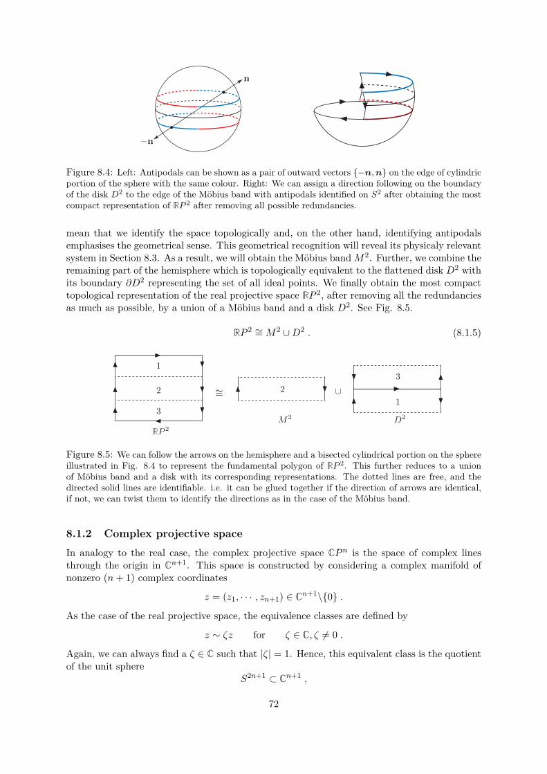
Figure 8.4: Left: Antipodals can be shown as a pair of outward vectors −n,n on the edge of cylindricportion of the sphere with the same colour. Right: We can assign a direction following on the boundaryof the disk D2 to the edge of the Möbius band with antipodals identified on S2 after obtaining the mostcompact representation of RP 2 after removing all possible redundancies.
mean that we identify the space topologically and, on the other hand, identifying antipodalsemphasises the geometrical sense. This geometrical recognition will reveal its physicaly relevantsystem in Section 8.3. As a result, we will obtain the Möbius band M2. Further, we combine theremaining part of the hemisphere which is topologically equivalent to the flattened disk D2 withits boundary ∂D2 representing the set of all ideal points. We finally obtain the most compacttopological representation of the real projective space RP 2, after removing all the redundanciesas much as possible, by a union of a Möbius band and a disk D2. See Fig. 8.5.
RP 2 ∼= M2 ∪D2 . (8.1.5)
∼=
Figure 8.5: We can follow the arrows on the hemisphere and a bisected cylindrical portion on the sphereillustrated in Fig. 8.4 to represent the fundamental polygon of RP 2. This further reduces to a unionof Möbius band and a disk with its corresponding representations. The dotted lines are free, and thedirected solid lines are identifiable. i.e. it can be glued together if the direction of arrows are identical,if not, we can twist them to identify the directions as in the case of the Möbius band.
8.1.2 Complex projective space
In analogy to the real case, the complex projective space CPn is the space of complex linesthrough the origin in Cn+1. This space is constructed by considering a complex manifold ofnonzero (n+ 1) complex coordinates
z = (z1, · · · , zn+1) ∈ Cn+1\0 .
As the case of the real projective space, the equivalence classes are defined by
z ∼ ζz for ζ ∈ C, ζ = 0 .
Again, we can always find a ζ ∈ C such that |ζ| = 1. Hence, this equivalent class is the quotientof the unit sphere
S2n+1 ⊂ Cn+1 ,
72
which can be seen from the fact that
S2n+1 ⊂ R2(n+1) ∼= Cn+1 .
But vectors in S2n+1 ⊂ Cn+1, with its last component is real and non-negative, are preciselyvectors of the form
(ω,√
1 − |ω|2) ∈ Cn × C, |ω| ≤ 1 .
In particular, we can regard this as a disk D2n bounded by the sphere S2n+1 if it consists ofvectors
(ω, 0) ∈ Cn × C, |ω| = 1 ,where we used the identifications of spheres, disks and its boundaries for a given Rn+1 by
Sn ⊂ Rn+1, Dn ⊂ Rn, ∂Dn = Sn−1 .
Hence, each vector in S2n+1 is equivalent under the identifications z ∼ ζz to a vector in D2n
and the vectors are unique if its last component is nonzero. If the last coordinate is zero, wecan always have the identifications z ∼ ζz for z ∈ S2n−1. In other words, every line in Cn+1
intersects the unit sphere in a circle and we can write
CPn ∼= S2n+1/S1 . (8.1.6)
This is analogous to the real projective space (8.1.3) in which the quotient space is taken by theset of antipodals. So, the difference between the real and the complex projective space arisesby identifying the equivalence classes in each space of Rn+1 and Cn+1, in such a way that
RPn ⊂ Rn+1 : x ∼ λx |λ| = 1, λ ∈ R antipodalsCPn ⊂ Cn+1 : z ∼ ζz |ζ| = 1, λ ∈ C S1 .
(8.1.7)
Moreover, a pair of antipodals in the real and the complex projective spaces are invariant underdiscrete symmetry x → −x and under SO(2), respectively.
8.1.3 Homotopy and projective space
The principal fibre bundle structure E,M,G, π, ψ consists of total space E and its projectedbase space M by a map π. The action of the group G is defined on the total space by a mapψ : E ×G −→ E. With a notion of fibre bundle F , it is conveniently expressed by a sequentialexpression
F → E → M . (8.1.8)We note that the complex projective space CPn carries the structure of a complex manifoldof Cn and the structure of a real manifold R2n. In particular, if n = 1 the complex projectivespace CP 1 is identified with the Riemann sphere. This is known as the Hopf fibration, andits fibre bundle structure is conventionally written by
S1 → S3 → CP 1 . (8.1.9)
In general, we summarise some important fibrations as follows.
SO(n− 1) → SO(n) → Sn−1 , (8.1.10a)SU(n− 1) → SU(n) → S2n−1 , (8.1.10b)S0(= Z2) → Sn → RPn , (8.1.10c)
S1 → S2n+1 → CPn . (8.1.10d)
73
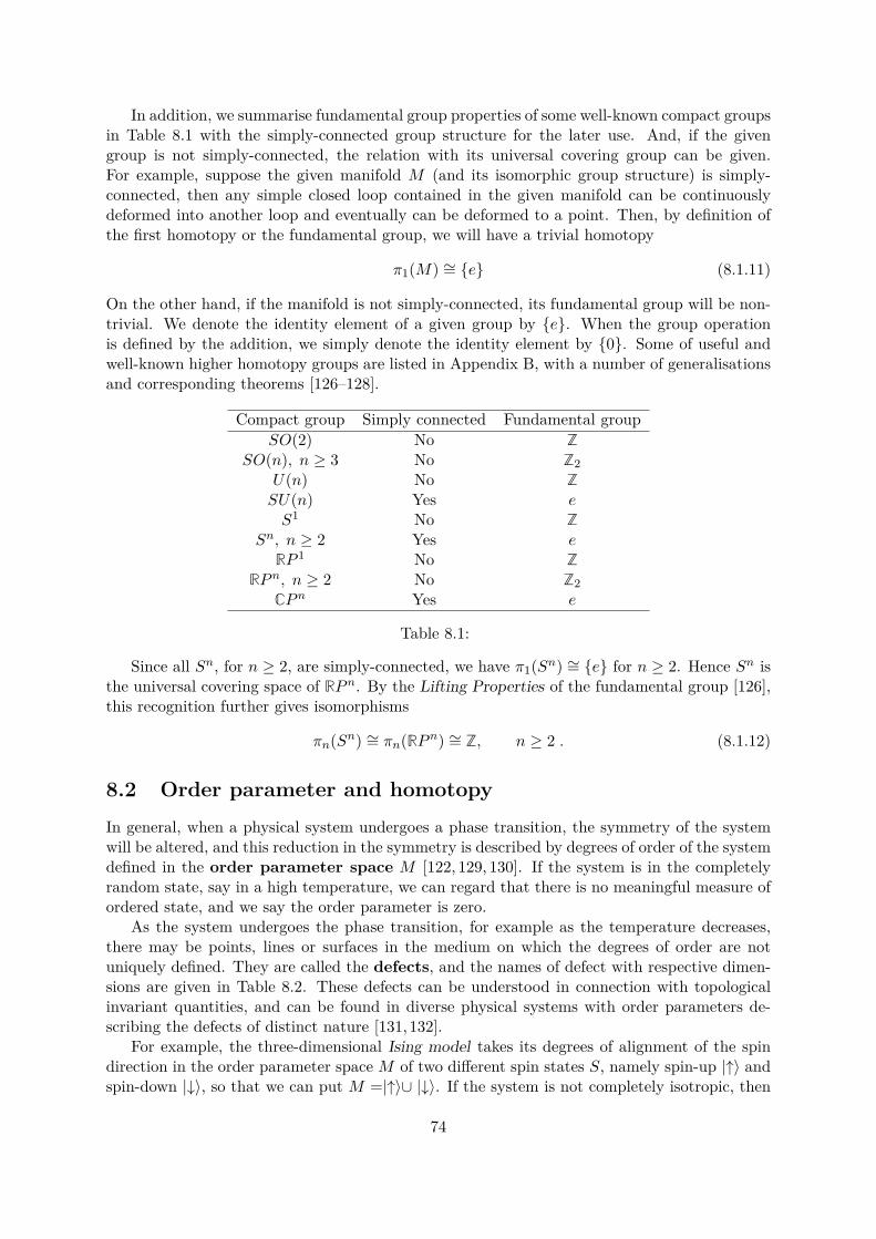
In addition, we summarise fundamental group properties of some well-known compact groupsin Table 8.1 with the simply-connected group structure for the later use. And, if the givengroup is not simply-connected, the relation with its universal covering group can be given.For example, suppose the given manifold M (and its isomorphic group structure) is simply-connected, then any simple closed loop contained in the given manifold can be continuouslydeformed into another loop and eventually can be deformed to a point. Then, by definition ofthe first homotopy or the fundamental group, we will have a trivial homotopy
π1(M) ∼= e (8.1.11)
On the other hand, if the manifold is not simply-connected, its fundamental group will be non-trivial. We denote the identity element of a given group by e. When the group operationis defined by the addition, we simply denote the identity element by 0. Some of useful andwell-known higher homotopy groups are listed in Appendix B, with a number of generalisationsand corresponding theorems [126–128].
Compact group Simply connected Fundamental groupSO(2) No Z
SO(n), n ≥ 3 No Z2U(n) No ZSU(n) Yes eS1 No Z
Sn, n ≥ 2 Yes eRP 1 No Z
RPn, n ≥ 2 No Z2CPn Yes e
Table 8.1:
Since all Sn, for n ≥ 2, are simply-connected, we have π1(Sn) ∼= e for n ≥ 2. Hence Sn isthe universal covering space of RPn. By the Lifting Properties of the fundamental group [126],this recognition further gives isomorphisms
πn(Sn) ∼= πn(RPn) ∼= Z, n ≥ 2 . (8.1.12)
8.2 Order parameter and homotopyIn general, when a physical system undergoes a phase transition, the symmetry of the systemwill be altered, and this reduction in the symmetry is described by degrees of order of the systemdefined in the order parameter space M [122, 129, 130]. If the system is in the completelyrandom state, say in a high temperature, we can regard that there is no meaningful measure ofordered state, and we say the order parameter is zero.
As the system undergoes the phase transition, for example as the temperature decreases,there may be points, lines or surfaces in the medium on which the degrees of order are notuniquely defined. They are called the defects, and the names of defect with respective dimen-sions are given in Table 8.2. These defects can be understood in connection with topologicalinvariant quantities, and can be found in diverse physical systems with order parameters de-scribing the defects of distinct nature [131,132].
For example, the three-dimensional Ising model takes its degrees of alignment of the spindirection in the order parameter space M of two different spin states S, namely spin-up |↑⟩ andspin-down |↓⟩, so that we can put M =|↑⟩∪ |↓⟩. If the system is not completely isotropic, then
74
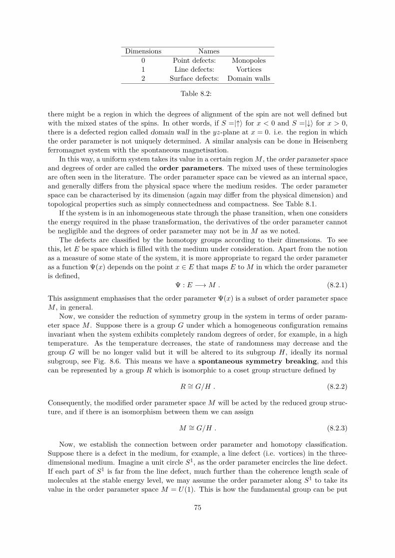
Dimensions Names0 Point defects: Monopoles1 Line defects: Vortices2 Surface defects: Domain walls
Table 8.2:
there might be a region in which the degrees of alignment of the spin are not well defined butwith the mixed states of the spins. In other words, if S =|↑⟩ for x < 0 and S =|↓⟩ for x > 0,there is a defected region called domain wall in the yz-plane at x = 0. i.e. the region in whichthe order parameter is not uniquely determined. A similar analysis can be done in Heisenbergferromagnet system with the spontaneous magnetisation.
In this way, a uniform system takes its value in a certain region M , the order parameter spaceand degrees of order are called the order parameters. The mixed uses of these terminologiesare often seen in the literature. The order parameter space can be viewed as an internal space,and generally differs from the physical space where the medium resides. The order parameterspace can be characterised by its dimension (again may differ from the physical dimension) andtopological properties such as simply connectedness and compactness. See Table 8.1.
If the system is in an inhomogeneous state through the phase transition, when one considersthe energy required in the phase transformation, the derivatives of the order parameter cannotbe negligible and the degrees of order parameter may not be in M as we noted.
The defects are classified by the homotopy groups according to their dimensions. To seethis, let E be space which is filled with the medium under consideration. Apart from the notionas a measure of some state of the system, it is more appropriate to regard the order parameteras a function Ψ(x) depends on the point x ∈ E that maps E to M in which the order parameteris defined,
Ψ : E −→ M . (8.2.1)
This assignment emphasises that the order parameter Ψ(x) is a subset of order parameter spaceM , in general.
Now, we consider the reduction of symmetry group in the system in terms of order param-eter space M . Suppose there is a group G under which a homogeneous configuration remainsinvariant when the system exhibits completely random degrees of order, for example, in a hightemperature. As the temperature decreases, the state of randomness may decrease and thegroup G will be no longer valid but it will be altered to its subgroup H, ideally its normalsubgroup, see Fig. 8.6. This means we have a spontaneous symmetry breaking, and thiscan be represented by a group R which is isomorphic to a coset group structure defined by
R ∼= G/H . (8.2.2)
Consequently, the modified order parameter space M will be acted by the reduced group struc-ture, and if there is an isomorphism between them we can assign
M ∼= G/H . (8.2.3)
Now, we establish the connection between order parameter and homotopy classification.Suppose there is a defect in the medium, for example, a line defect (i.e. vortices) in the three-dimensional medium. Imagine a unit circle S1, as the order parameter encircles the line defect.If each part of S1 is far from the line defect, much further than the coherence length scale ofmolecules at the stable energy level, we may assume the order parameter along S1 to take itsvalue in the order parameter space M = U(1). This is how the fundamental group can be put
75
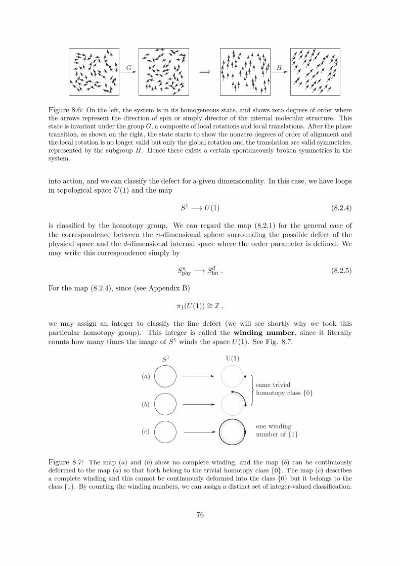
=⇒
Figure 8.6: On the left, the system is in its homogeneous state, and shows zero degrees of order wherethe arrows represent the direction of spin or simply director of the internal molecular structure. Thisstate is invariant under the group G, a composite of local rotations and local translations. After the phasetransition, as shown on the right, the state starts to show the nonzero degrees of order of alignment andthe local rotation is no longer valid but only the global rotation and the translation are valid symmetries,represented by the subgroup H. Hence there exists a certain spontaneously broken symmetries in thesystem.
into action, and we can classify the defect for a given dimensionality. In this case, we have loopsin topological space U(1) and the map
S1 −→ U(1) (8.2.4)
is classified by the homotopy group. We can regard the map (8.2.1) for the general case ofthe correspondence between the n-dimensional sphere surrounding the possible defect of thephysical space and the d-dimensional internal space where the order parameter is defined. Wemay write this correspondence simply by
Snphy −→ Sd
int . (8.2.5)
For the map (8.2.4), since (see Appendix B)
π1(U(1)) ∼= Z ,
we may assign an integer to classify the line defect (we will see shortly why we took thisparticular homotopy group). This integer is called the winding number, since it literallycounts how many times the image of S1 winds the space U(1). See Fig. 8.7.
Figure 8.7: The map (a) and (b) show no complete winding, and the map (b) can be continuouslydeformed to the map (a) so that both belong to the trivial homotopy class 0. The map (c) describesa complete winding and this cannot be continuously deformed into the class 0 but it belongs to theclass 1. By counting the winding numbers, we can assign a distinct set of integer-valued classification.
76
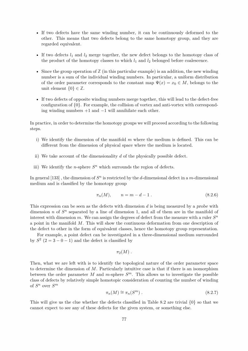
• If two defects have the same winding number, it can be continuously deformed to theother. This means that two defects belong to the same homotopy group, and they areregarded equivalent.
• If two defects l1 and l2 merge together, the new defect belongs to the homotopy class ofthe product of the homotopy classes to which l1 and l2 belonged before coalescence.
• Since the group operation of Z (in this particular example) is an addition, the new windingnumber is a sum of the individual winding numbers. In particular, a uniform distributionof the order parameter corresponds to the constant map Ψ(x) = x0 ∈ M , belongs to theunit element 0 ∈ Z.
• If two defects of opposite winding numbers merge together, this will lead to the defect-freeconfiguration of 0. For example, the collision of vortex and anti-vortex with correspond-ing winding numbers +1 and −1 will annihilate each other.
In practice, in order to determine the homotopy groups we will proceed according to the followingsteps.
i) We identify the dimension of the manifold m where the medium is defined. This can bedifferent from the dimension of physical space where the medium is located.
ii) We take account of the dimensionality d of the physically possible defect.
iii) We identify the n-sphere Sn which surrounds the region of defects.
In general [133] , the dimension of Sn is restricted by the d-dimensional defect in am-dimensionalmedium and is classified by the homotopy group
πn(M), n = m− d− 1 . (8.2.6)
This expression can be seen as the defects with dimension d is being measured by a probe withdimension n of Sn separated by a line of dimension 1, and all of them are in the manifold ofinterest with dimension m. We can assign the degrees of defect from the measure with a ruler Sn
a point in the manifold M . This will show the continuous deformation from one description ofthe defect to other in the form of equivalent classes, hence the homotopy group representation.
For example, a point defect can be investigated in a three-dimensional medium surroundedby S2 (2 = 3 − 0 − 1) and the defect is classified by
π2(M) .
Then, what we are left with is to identify the topological nature of the order parameter spaceto determine the dimension of M . Particularly intuitive case is that if there is an isomorphismbetween the order parameter M and m-sphere Sm. This allows us to investigate the possibleclass of defects by relatively simple homotopic consideration of counting the number of windingof Sn over Sm
πn(M) ∼= πn(Sm) . (8.2.7)
This will give us the clue whether the defects classified in Table 8.2 are trivial 0 so that wecannot expect to see any of these defects for the given system, or something else.
77

8.3 Nematic liquid crystalsCertain organic crystals exhibit quite interesting optical properties when they are in the isotropicfluid phases in which orientations and positions of directors are randomly distributed. Theyare called liquid crystals, characterized by their optical features. We are particularly interestedin the so-called nematic liquid crystals. These are characterised by its long axes orientedalong a certain direction while the positions of the centre of individual molecule are isotropic.An example of this is would be Octyloxy-Cyanobiphenyl. See Fig. 8.8.
Figure 8.8: Left: By following a pair of antipodals on the cylindrical portion in constructing the Möbiusband on S2, it is easy to associate opposite signed directors n and −n on the sphere. Right: A moleculemodel of rod-like shaped Octyloxy-Cyanobiphenyl with chemical formula C21H25NO is shown with oneoxygen atom in the middle (red) and one nitrogen atom attached in the end (blue) among the compoundof hydrogen and carbon molecules in the aligned bulk along the direction of vector nN.
In this case, we can take the order parameter M as the measure of the degree of alignmentamong the molecules, and is proportional to the director aligned to a vector nN. And it is givenby the average direction of the rigid rod-like molecular structure. This suggests the rotationalsymmetry is broken while the translational symmetry still holds through the symmetry reductionprocess from the completely random state. Although the molecule possesses the apparentlydistinguishable head and tail feature, we do not distinguish the directors. i.e. If the moleculesare aligned in one direction, then it possesses the discrete symmetry, nN → −nN. We mightassume that this vector is normalised, so that
nN · nN = 1 . (8.3.1)
Further, if we assign a point of the nematic liquid crystal x ∈ R3, we can express a pair ofidentifiable directors in the polar coordinate system,
nN = (θ, ϕ) and − nN = (π − θ, π + ϕ) . (8.3.2)
From (8.2.7) and (8.3.2), we can see these constitute a point on S2 ⊂ R3 representing the samestate. We see that the identification of nN = −nN is nothing but the identification of theantipodals on S2. Therefore the order parameter space of the nematic liquid crystals is theprojective plane RP 2.
In general, the director field depends on the position x ∈ S2 ⊂ R3 and we may define a mapfollowing (8.2.1),
Ψ : S2 −→ RP 2 . (8.3.3)This particular example emphasises the difference between the space S2 where the mediumexists and the order parameter space RP 2 due to the identification nN = −nN. This map iscalled the texture. Sometimes, the actual order parameter configuration in R3 is also called thetexture.
78
If we bring back the construction of the Möbius band in Section 8.1, we recognise the topo-logical identification of antipodals directly corresponds to the identification of the geometricaland physical identification of directors nN = −nN. See Fig. 8.8. Therefore, using (8.1.12), wecan write an expression for the general homotopy group, now the order parameter space M isrecognised,
πn(S2/antipodal) ∼= πn(RP 2) . (8.3.4)
Let us investigate various possible defects whether (8.3.4) gives us any meaningful indication.For the line defects, we have the dimension d = 1 and the dimension of media is m = 3. So thatn = 3 − 1 − 1 = 1, and this gives the first homotopy group we can work with,
π1(RP 2) ∼= Z2 = 0, 1 . (8.3.5)
This implies that there exist two kinds of line defect in nematic liquid crystals [69,123,124,133],
0 : one can be continuously deformed into a uniform configuration,1 : one cannot be continuously deformed into a uniform configuration.
(8.3.6)
The latter represents non-trivial defect, a stable vortex, and we can see how the loop is mappedto RP 2 by this texture.
For the point defect, we can consider the case for m = 3, d = 0 and n = 3 − 0 − 1 = 2, sothat the corresponding homotopy group is now
π2(S2) ∼= π2(RP 2) ∼= Z . (8.3.7)
where we used (8.1.12). This indicates that there are stable point defects in the nematic liquidcrystals classified by some integers, and this classification can be equally applied to the fieldconfiguration defined on S2. This idea of linking an integer with homotopy group is a centralingredient to represent the topological invariants that we will see in Section 9.2.
In this way, in principle we can investigate the classifications of defects in various physicalmodels, after defining i) the order parameters and ii) the order parameter space by recognisingthe underlying symmetries in the system in each case. In particular, we would like to consider thehomotopy and the physical meaning of RP 3 with its topological implication. This is essentiallythe generalisation of the nematic liquid crystals case. Before that, we shall go back to the notionof directors in micropolar theory and its characteristic deformational measures to consider theenergy functions within the framework of the free energy formalism.
8.4 Free energy formalism and its expansion
8.4.1 Order parameters in the energy expansion
External factors such as a temperature, chemical interaction, an electromagnetic field or agravitational field can induce the phase transition and the order parameter acquires nonzerovalues, if one started from the completely random state, defined in certain order parameterspace. Then it is natural to expect that some of symmetric properties in the isotropic state arebroken during the phase transition, and the energy density can be expressed as a function ofthe field of the order parameter.
The free energy formalism for the liquid crystals was established by Oseen [134] and Frank[135]. Later the theory was further developed by Ericksen and Leslie [136–138], incorporatinginequalities in the nematic liquid crystals within the framework of the continuum theory. Thefree energy formalism is based on the notion of the energy required for deviations from the
79
isotropic state in which the order parameter is taken to be zero [139]. This immediately suggeststhat we can take the director ξa as the order parameter to investigate potential deformations(or deviations from the initial state). Therefore, the energy density must be proportional to thederivative of the order parameter,
F ∝ (∇ξa)2 . (8.4.1)
The free energy density can be written in terms of the power expansion of the order param-eter and its derivatives, under the assumption that the spatial variations are slow relative to thecharacteristic length scale, for example, the range of interaction or the coherent length in thelattice space for a given system. This form of expansion is highly dependent on the nature ofthe order parameter itself in the given physical system. It can be a single real scalar parameteror an n-component complex field. But we are particularly interested in its simple form of freeenergy expansion in the case of nematic liquid crystals given in terms of the directors.
For the nematic liquid crystals, the energy expansion is written by the linear expansionof the polynomial of the order parameter Q up to finite powers to ensure the stability of thesystem and its derivative combinations [32, 140]. In each expansion of the energy function, the3×3 matrix Q is known as traceless and symmetric written in such a way that each term in theexpansion of F is invariant individually under the global rotation. Terms containing derivativeoperator of Q are called the gradient free energy, and it is written up to second order. Andterms without the derivative operator are known as the bulk free energy up to fourth order, sothat the free energy density is written as
F = Fbulk + Fgrad . (8.4.2)
Specifically, we can write the expansion [141] with some elastic moduli ki
Fbulk = k1tr Q2 + k2tr Q3 + k3[tr Q2]2 , (8.4.3a)Fgrad = k4 (∇ × Q + k5Q)2 + k6 (∇ · Q)2 . (8.4.3b)
where we can rewrite the fourth power term in (8.4.3a) by tr Q4 = 12 [tr Q2]2, for Q is 3 × 3
traceless matrix.Now, we would like to specify the form of the order parameter Q which must be a function
of the director nN, and it must be zero when the system is in the completely random state losingall its degrees of alignment, so that it is no longer the nematic but in an isotropic configuration.There are number of approaches in the literature to determine the order parameter Q, but wewould like to take one that can encompass the theory of the microcontinuum.
The relation of vanishing order parameter and the resulting isotropic configuration can befound in consideration of the so-called microinertia defined by Eringen [142]. The microinertiafor micropolar continua is defined by
jij = χiAχjBJAB , (8.4.4)
where jij and JAB are microinertia described by the directors ξk and ΞK in the spatial frameand reference frame respectively, and we identify χiA as the microrotation of SO(3) followingthe discussion in Section 6.3. A special case arises when we have jij = JAB. Then this meansthe microinertia is conserved regardless of the choice of the local microrotational axis, and thesystem is in the isotropic configuration. Further, since χχT = 1, the expression (8.4.4) becomes
jχ = χj .
Using the Schur’s Lemma [143], we can regard the microinertia as the map of the finite-dimensional vector space V to itself. So that for a nonzero eigenvector v ∈ V with a nonzero
80
eigenvalue λ ∈ R, jv = λv implies j(χv) = χ(jv) = λχv for all v ∈ V . Therefore theeigenspace is invariant under the microrotation as expected and j must be proportional to theidentity. Hence, we can write the microinertia in the form
jij = 23jkkδij . (8.4.5)
Now, in the nematic state, this microinertia will be modified to take the form, according to [142]
jij = σ(δij − nNinNj) (8.4.6)
where σ is some constant, and nNi are normalised directors satisfying nN · nN = 1. Then wecan determine the form of the order parameter Qij as the measure of its deviation from theisotropic state by
Qij = 23jkkδij − jij
=(nNinNj − 1
3δij
)σ
(8.4.7)
which is traceless and symmetric. And we can confirm that Qij → 0 when the system approachesthe isotropic state jij → 2
3jkkδij as expected.If we insert the form of the order parameter Qij of (8.4.7) into the free energy F (8.4.2),
then the form of F will be written entirely in terms of the directors nN and its derivatives [141],
F = 12K1[∇ · nN]2 + 1
2K2 [nN · (∇ × nN)]2 + 12K3[nN × (∇ × nN)]2 , (8.4.8)
where Ki are some material constants relating ki in (8.4.3), and the higher order terms areignored. Also, we dropped the surface terms knowing that the total energy function is obtainedafter the volume integration accompanied by the density constant. Each term attributes formsof defects, namely, splay (divergence), bend (curvature) and twist (torsion) terms, respectively,
[∇ · nN]2, [nN × (∇ × nN)]2, [nN · (∇ × nN)]2 , (8.4.9)
satisfying a set of required symmetries in the energy function. We can see that these satisfy theglobal rotation and the discrete symmetry nN → −nN. In particular, it is widely known [140]that if the system requires the chirality such as cholesteric liquid crystals, we need an additionalenergy term
nN · (∇ × nN) , (8.4.10)
with an appropriate coupling parameter.Similar form of the free energy formalism can be found in the general Ginzburg-Landau
expansion [144], if the systems satisfying certain criteria, for example, when the order parameteris small and uniform near the critical temperature Tc during the phase transition.
Some useful identities in the expansion are
(∇n)2 = (∇ · n)2 + (∇ × n)2 + ∇ ·[(n · ∇)n − n(∇ · n)
], (8.4.11a)
[(n · ∇)n]2 = [n × (∇ × n)]2 , (8.4.11b)(∇ × n)2 = [n · (∇ × n)]2 + [n × (∇ × n)]2 . (8.4.11c)
81
8.4.2 Torsion terms in the energy expansion
Now, we are particularly interested in the twist term in connection with the term which playedthe central role in developing the torsion throughout Part I and Part II. This quantity isRT CurlR which can be related to the term nN ·(∇×nN) to investigate the torsion contributionto the given system with the energy configuration as the invariant linear combinations of thoseterms. For instance, we can derive the form of the free energy functional as discussed in [15] tocompare the energy functionals we used in (2.1.1) and (3.4.2). So, the first step is to establishthe relationship between
RT CurlR and nN · (∇ × nN) . (8.4.12)
We would like to look closely at the rotational matrix to investigate the role of its axis andthe angle for our purpose. The matrix R ∈ SO(3), describing the rotation of the angle θ aboutthe normalised axis n, can be expressed as the exponential of the antisymmetric matrix A,
R = eA for AT = −A . (8.4.13)
where the matrix A can be written
Aij = θ(n · J) ≡ θaij (8.4.14)
and the generators J = (J1, J2, J3) of SO(3) are
J1 =
0 0 00 0 −10 1 0
, J2 =
0 0 10 0 0
−1 0 0
, J3 =
0 −1 01 0 00 0 0
(8.4.15)
satisfying the commutation relation,
[Ji, Jj ] = ϵijkJk . (8.4.16)
The axial vector ni for the rotation is defined by
ni = −12ϵijkajk and aij = −ϵijknk . (8.4.17)
Both variables of ni and θ can be arbitrary functions of space x = (x, y, z) and time t, butwe only consider the static case so that both axis and rotational angle are time-independentfunctions. We can write the rotational axis by
n = (n1(x), n2(x), n3(x)) satisfying n · n = 1 . (8.4.18)
There are number of known representations for the rotation R, and one of them is Rodrigues’formula
Rij = δij + aij sin θ + (a2)ij(1 − cos θ) . (8.4.19)
Using the fact that (a2)ij = aikakj = −δijnlnl + ninj , we can write the equivalent expression,
Rij = cos θ · δij + ninj(1 − cos θ) − ϵijmnm sin θ . (8.4.20)
We note that because of the normalisation constraint n21 + n2
2 + n23 = 1, the total number of
independent parameters required is three, which agrees with the number of generators J in(8.4.15). These representations of matrices Aij and Rij are particularly useful if one considers
82
an anisotropic system. For example, in the planar case, the axial vector n can be perpendicularto the director fields which might give rise to the solution that minimises the energy function.
Now, we return to the issue of relating RT∂R and nN · (∇ × nN). Intuitively, one mighthope to write the contortion (6.2.3) by
Kpiq = Rdp∂iRdq = R−1∂iR = ∂i log R = ∂iApq . (8.4.21)
when the rotation is expressed by the exponential form of the antisymmetric matrixA of (8.4.13).This is not true in general, simply because in the matrix Aij = θaij = −ϵijknkθ, the rotationalangle θ and the axis n are position-dependent functions. Nonetheless, if the angle θ is small,using the definition of contortion with the exponential representation of rotation R = eA, wecan show that
Kpiq ≈ ∂iApq . (8.4.22)
But, if the normalised rotational axis is constant in space, which is the case we have seen in PartI of (2.2.1), while the rotational angle can be an arbitrary function of space, then the contortiontensor can be written exactly as
Kpiq = ∂iApq . (8.4.23)
To see this, first we write an N product of the generators A of R ∈ SO(3)
(AN )ij = θail1θal1l2 · · · θalnn = θNa1l1 · · · alnj ,
with its derivative∂m(AN )in = ail1 · · · alnn∂mθ
N = N(AN−1∂mA) .
Using this, the contortion K = RT∂R becomes
Kpiq = (eA)T(
1 +A+ 12!A
2 + · · ·)∂iA
= (eA)T eA∂iA
(8.4.24)
which gives the result, for RTR = 1. In particular, the dislocation density tensor (6.2.5) andNye’s tensor (6.2.8) simply become,
Kpj = δjp∂iθni − ∂pθnj , (8.4.25a)Γji = ∂iθnj . (8.4.25b)
Further, the torsion tensor defined by Tipq = Γipq − Γiqp in (5.2.1) can be written in termsof the contortion tensor under the assumption that U b
µ = δbµ in the decomposition (5.2.2),
Tpiq = apq∂iθ − api∂qθ . (8.4.26)
In other words, the torsion tensor can be written as the gradient of the scalar field if therotational axis do not change in space. Torsion as the gradient of the scalar field is discussedextensively in [75].
In Weitzenböck space (i.e. the space of zero curvature but nonzero torsion), the generalaffine connection is identified with the contortion tensor, so the Riemann curvature tensor canbe written entirely with the contortion tensor. Then, a straightforward calculation using (8.4.23)and (8.4.14), gives the expression (6.2.4)
Rρσµν = ∂µKρνσ − ∂νKρµσ +KρµλKλνσ −KρνλKλµσ (8.4.27)
which again agrees with the result we obtained in Section 6.2.
83
Now, in the language of the micropolar deformation, we can relate the directors ξa and rota-tions R with respect to the orthonormal basis ei in the Cartesian coordinate system, followingsimilar reasoning used in [142, 145, 146]. We may assign the tetrad field Eµ
a ∈ GL(3; R) and itsdual ea
µ, the χkK and its inverse in (1.2.20), in describing the transformations of the directorsin the spatial frame and the reference frame to write
ξa = Eµa Ξµ and Ξµ = ea
µξa . (8.4.28)
In the case of micropolar continua, according to the decompositions (6.3.3a) and (6.3.4b), thetransformation can be described only by the microrotation so that ξa = Ra
µΞµ, or vice versa.The director Ξµ, as the description of the internal structure, is highly dependent on the individ-ual molecular structure. However, if we have a model such as cubane as shown in Fig. 1.1, wemay put the director in the reference frame to the usual orthonormal Cartesian basis to write
ξc = Rcbeb . (8.4.29)
i.e. we can regard that the director ξa is obtained after applying the rigid rotation to thestandard orthonormal basis in three dimensions. Then the contortion becomes
Kaµb = Rca∂µRcb = ξa∂µξb . (8.4.30)
Consequently, the dislocation density tensor becomes
Kad = ϵdµbKaµb = ξaϵdµb∂µξb = ξa(Curl ξ)d . (8.4.31)
And Nye’s tensor becomes
Γji = −12ϵjpqKpiq = −1
2ϵjpqξp∂iξq . (8.4.32)
Now, it becomes clear that the quantity corresponding to the twist in (8.4.8) [ξ · (Curl ξ)] isthe trace of the dislocation density tensor
tr K = [ξ · (Curl ξ)] . (8.4.33)
Furthermore, from the relation between Nye’s tensor and the dislocation density tensor (6.2.11),we obtain the explicit relation between Nye’s tensor and the measure for the twist, as givenin [142] and [145]
tr Γ = 12tr K = 1
2ξ · (Curl ξ) . (8.4.34)
We also note that (8.4.33) and (8.4.34) are precisely the simplest form of the chiral energyform we discussed in Section 3.3,
Vχ = χtr(K). (8.4.35)
In words, a system with no mirror symmetry is defined by the chirality, and this system mustaccompanied by the chiral energy form Vχ which in turn induced by nonzero torsion in the formeither by the dislocation density tensor or Nye’s tensor via contortion tensor. Consequently, forsuch a system the parameter, now we can set k5 = χ, is nonzero in (8.4.3b).
In case of nematic liquid crystals [142, 146], the directors nN are obtained simply followingthe same reasoning of (8.4.29) but by fixing ei to be e3,
nNi = Ri3e3 . (8.4.36)
84
In this way, it is easy to see that the result we obtained so far can be translated into the formssuch as
ξ · (Curl ξ) −→ nN · (∇ × nN) . (8.4.37)
Then it is straightforward to see that the nematic liquid crystals are in its homogeneousanisotropic configuration seen as the special case of micropolar theory, as claimed by Erin-gen in [142]. In particular, the term with K2 on the right hand side of (8.4.8) is in its evenpower of (8.4.37). This manifests that the energy functional for the liquid nematic crystals isthe non-chiral case, following the conclusion of Section 3.3. Therefore, we can set the constantk5 = 0 in (8.4.3b).
8.4.3 Order parameter for the micropolar continua
Lastly, we would like to make some remarks on the equation of motion for the general micropolarcontinua obtained in Chapter 2 in connection with those in [15].(∂ttϕ∂ttψ
)= M
(∂zzϕ∂zzψ
)+(
0 λ sin ϕ2ρrot
−2λ sin ϕρ 0
)(∂zϕ∂zψ
)− (λ+ µ+ µc)
ρrot
(sinϕ
0
)+ λ+ µ
2ρrot
(sin 2ϕ
0
)(8.4.38a)(
∂ttϕ∂ttu
)= N
(∂xxϕ∂xxu
)+(
0 2λ′ sin ϕρ0J
−2(λ′+2µ′+κ′) sin ϕρ0
0
)(∂xϕ∂xu
)+ 2λ′
ρ0J
(sinϕ
0
)+ 2λ′ + µ′
ρ0J
(sin 2ϕ
0
)(8.4.38b)
where
M =(
(κ1 + 6κ3)/3ρrot (3χ1 − χ3)/6ρrot2(3χ1 − χ3)/3ρ (λ+ 2µ)/ρ
), N =
(α
ρ0J 00 λ′+2µ′+κ′
ρ0
). (8.4.39)
In our case, we obtained the equations of motion by collecting all relevant energy functionalsin terms of the microrotation and the macro-displacement. And the variational principle ledto (8.4.38a). For (8.4.39b), it is based on the different approach starting from the constitutiveequations for the micropolar media and identifying two order parameters CKL and ΓKL in thefree energy density F given by
TKl = ∂F∂CKL
χlL and MKl = ∂F∂ΓLK
χlL , (8.4.40)
where Piola-Kirchhoff tensors are defined by
TKl = J∂XK
∂xktkl and MKl = J
∂XK
∂xkmkl
for tkl and mkl are the stress tensor and the couple tensor, respectively, and the determinantJ is given by (1.2.22). The free energy density (8.4.8) is then given by the simplified linearexpansion of powers of two order parameters [146, 147], with the aids of identities (8.4.11), inthe form
F = 12λ
′I21 + µ′I2 + (µ′ + κ′)I4 + 1
2α′I10 + β′I11 − γ′I13 (8.4.41)
where λ′, µ′, κ′, α′, β′, γ′ are some elastic parameters. The invariants in (8.4.41) are
I1 = tr C, I2 = 12tr C2, I4 = 1
2tr (CCT ) ,I10 = tr Γ, I11 = 1
2tr Γ2, I13 = 12tr (ΓΓT ) . (8.4.42)
85
The appearance of two different kinds of order parameters of the first Cosserat deformationtensor C and Nye’s tensor Γ in the expansion explains the setting we are dealing with. Thisis the coupled system of micro and macro-deformations leading to the two deformational wavepropagations. Moreover, the constitutive equations (8.4.40) is of the form we used in (2.0.1),and the identification between the trace of Nye’s tensor and the dislocation density tensor interms of the twist measure of the director explains the similarity.
In a sense, our formalism (2.0.1) in varying the total energy functional in terms of themicrorotation R and the deformation gradient tensor F , is equivalent to the formalism basedon the constitutive equations (8.4.40). The chain rules introduced in Appendix A would beparticularly useful in varying the first Cosserat deformation tensor (U = R
TF in our convention)
and Nye’s tensor (as the product of the microrotation and its derivative). This essentially leadsto the close similarity in the final coupled set of equations of motion as shown in (8.4.38).
In principle, one may adjust the parameters in the matrix M to obtain a diagonalisedmatrix to match the entries of the matrix N under certain circumstances in evaluating theconstitutive equations exactly. Then the simple ansatz, such as the microrotation with fixedaxis (2.2.1), can be imposed to yield the identical set of equations of motion from the ratherdifferent approaches. We note that while Nye’s tensor is extensively used as the order parameterin literature [15, 26, 142, 146], we can equally use the dislocation density tensor K as the orderparameter according to (8.4.34).
86
Chapter 9
Topological invariants and conservedcurrents
We would like reconsider the soliton solutions we obtained in Part I through some simple casesto investigate the relationship with the homotopy to classify the solution space in describingthe defects. This solution space can be arbitrarily large if there exist underlying symmetries ofinfinite order group structures.
Various systems which yield a soliton solution are introduced, and we will see that the finiteenergy requirement is the crucial feature in determining the asymptotic behaviour of the solitonsolutions and this will further be related to the homotopic classifications.
These asymptotic conditions are responsible for the existence of topological invariant chargesQ, and these topological invariants are different from the conventionally derived quantities, suchas Noether’s current, from the continuous symmetry in the Lagrangian of the system leading tothe conservation of energy and momentum. Depending on the physical system, this total chargeQ can be of the form of a mass, an electric charge or an intrinsic quantum number. Also thischarge will turn out to be a unique topological invariant in classifying the defects introduced inTable 8.2.
The associated conserved current is used extensively throughout Skyrme’s pioneering works.From a mathematical point of view, the theories of solitons are rigorously developed in variouscontexts in connection with the physical systems, and comprehensive discussions of the solitontheory can be found, for example, in [40].
9.1 Simple soliton solutions in low dimensions
In this Section, we will use the metric tensor with its signature (+1,−1, · · · − 1) in n spatialdimensions with one time component of the tensors defined in an (n+ 1)-dimensional differen-tiable manifold. For example, the Lorentzian metric tensor ηµν for µ, ν = t, x, y, z in (3 + 1)dimensions will give the invariant length element (5.1.6) (we put the speed of light c = 1)
(ds)2 = ηµνdxµdxν = (dt)2 − (dx)2 − (dy)2 − (dz)2 ,
and the indices of vectors are naturally raised and the indices of derivatives are naturally lowered.Let us start with a scalar field ϕ in a (1 + 1)-dimensional model without stating any specific
form of the Lagrangian. The zero dimensional sphere S0 is the set of two points which canbe taken to be x = ±∞. The corresponding homotopy group for the order parameter, using(8.2.3), is therefore
π0(M) ∼= π0(G/H) . (9.1.1)
87
This particular homotopy group counts the number of components of the order parameter spaceM . So, π0(M) is nonzero if M is discrete, or equivalently G is discrete. We will see that thisimplies that the disconnected groups impose (1 + 1)-dimensional soliton solutions.
Let us start with the currents for the scalar field ϕ defined by
Jµ = ϵµν∂νϕ (9.1.2)
where ϵµν is the totally antisymmetric Levi-Civita symbol in two dimensions with µ, ν for thespacetime indices in (1+1) dimensions. It is easy to see that this is conserved, by its construction
∂µJµ = 0 . (9.1.3)
And the corresponding total charge is defined by the integration of the time component of thecurrent J over all space,
Q =∫ ∞
−∞dx J t =
∫ ∞
−∞dx
∂ϕ
∂x= ϕ(+∞, t) − ϕ(−∞, t) . (9.1.4)
under the assumption that J t approaches zero as |x| → ∞, hence (9.1.4) states that a conservedcurrent implies a conserved charge in time. It is easy to show that the charge Q is a time-independent quantity, hence it possesses an intrinsic topological property.
For the finite energy requirement, the total charge must be localised. If the amplitude ofϕ(±∞, t) increases (or decreases) indefinitely or oscillates arbitrarily, we cannot expect to havethe finite-valued total charge. This will eventually violate the finite energy requirement for thegiven system, and it is required to set the asymptotic values for ϕ(x, t) to obtain the meaningfulphysical solution.
One solution for such condition would be the constant solution, but we can put this constantto be zero without loss of generality, so that the trivial solution is
ϕ(±∞, t) = 0 , (9.1.5)
to give Q = 0. But for the non-trivial case, we will have the nonzero-valued Q and we mighthave a situation that
ϕ(+∞, t) = ϕ(−∞, t) , (9.1.6)
where each ϕ(+∞, t) and ϕ(−∞, t) approaches distinct finite asymptotic values. This analysisagrees with the asymptotic condition we imposed in the case of elastic wave propagationsin (2.3.4). The distinct asymptotic values for ϕ(+∞, t) and ϕ(−∞, t) can impose differentinterpretation when we consider the elastic deformation.
Soliton solutions are characterised by their solitary wave form with non-dissipative termsand its interference-free properties from the collision or long-ranged interaction between distinctwaves. We would like to derive the soliton solutions similar to those we used in Part I, butthrough much simpler and familiar examples.
First, the Lagrangian for the ϕ4 theory of the real scalar field in (1 + 1) dimensions is
L = 12∂µϕ∂
µϕ+ 12µ
2ϕ2 − 14λϕ
4 , (9.1.7)
where we understood that ∂µϕ∂µϕ = (∂tϕ)2 − (∂xϕ)2 and µ, λ are real coupling constants. The
only symmetry in this system is O(1) ∼= Z2, which is simply the identity and its reflection,
ϕ −→ −ϕ . (9.1.8)
88
The homotopy group in this case is a map between the physically allowed space and the internalspace, therefore using (8.2.5) we have
π0(Z2) ∼= Z2 . (9.1.9)
Hence, we can expect that there are two classes of solutions, namely
ϕ(+∞, t) = ϕ(−∞, t) and ϕ(+∞, t) = ϕ(−∞, t) .
This shows that by following a simple reasoning on the structure of order parameter space Mand its associated symmetry, we can have some approximate ideas about the solution space wellbefore we actually tackle the equation of motion to solve it.
Now, the equation of motion can be obtained by
∂µ∂µϕ ≡ ∂2ϕ
∂t2− ∂2ϕ
∂x2 = µ2ϕ− λϕ3 (9.1.10)
with constant solutions for the first class of 0 ∈ Z2 yielding the zero charge Q, called a vacuumsolution,
ϕvac = 0 and ϕvac = ± µ√λ. (9.1.11)
For the solution of the second class ϕ(+∞, t) = ϕ(−∞, t), for the nonzero total charge, weconsider the static solution of (9.1.10), and this can be done by integrating both sides withrespect to x after multiplying by ∂ϕ/∂x, to obtain
x = ±∫ 1√
12λϕ
4 − µ2ϕ2 + kdϕ , (9.1.12)
for some constant k, and we put the integration constant to be zero. This is in the form of anelliptic integral, hence the solution ϕ can be periodic in the complex plane. But if we have therepeated roots in the square, we can integrate exactly, and this is the case when k = µ4/2λ.Then (9.1.12) reduces to a simple integration and we obtain the kink/antikink solution,
ϕkink(x) = ± µ√λ
tanh[µ√2x
]. (9.1.13)
Using the result we obtained in Section 2.5, we can obtain the time-dependent wave solutionpropagating with the velocity v, by applying the Lorentz boost in the direction of x providedthe Lagrangian is Lorentz invariant
ϕkink(x, t) = ± µ√λ
tanh[µ√2
1√1 − v2
(x− vt)]. (9.1.14)
It is clear that these solutions belong to the classification of ϕ(+∞, t) = ϕ(−∞, t), and theirasymptotic behaviour indicates that
ϕkink(x, t) −→ ϕvac as x → ±∞ .
This solution leads to the finite energy with respect to the vacuum, if we insert the kink solution(9.1.14) into the Hamiltonian H defined by the integration over the energy density H(x) of(2.5.3),
H =∫dx
(12
[(∂ϕ
∂t
)2+(∂ϕ
∂x
)2]− 1
2µ2ϕ2 + λ
4ϕ4). (9.1.15)
89
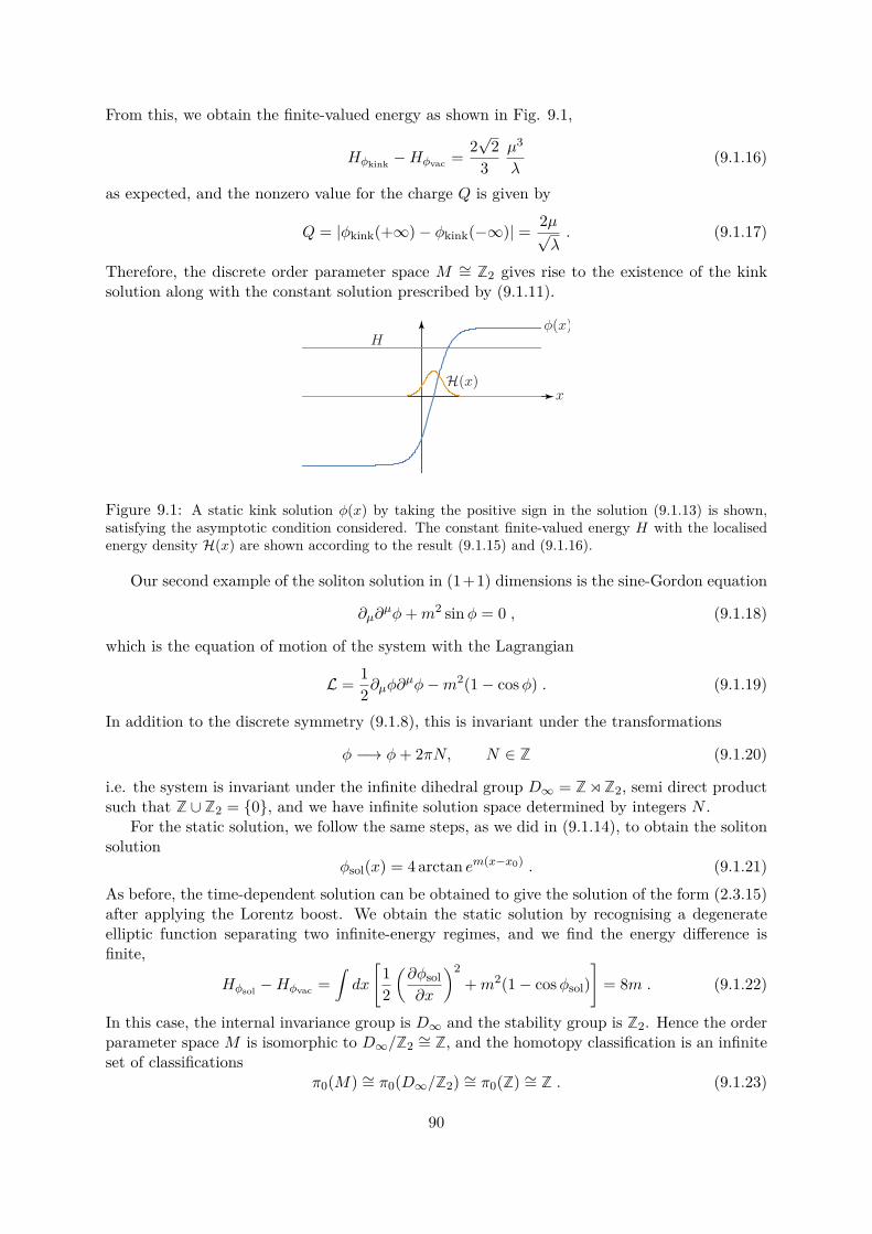
From this, we obtain the finite-valued energy as shown in Fig. 9.1,
Hϕkink −Hϕvac = 2√
23
µ3
λ(9.1.16)
as expected, and the nonzero value for the charge Q is given by
Q = |ϕkink(+∞) − ϕkink(−∞)| = 2µ√λ. (9.1.17)
Therefore, the discrete order parameter space M ∼= Z2 gives rise to the existence of the kinksolution along with the constant solution prescribed by (9.1.11).
Figure 9.1: A static kink solution ϕ(x) by taking the positive sign in the solution (9.1.13) is shown,satisfying the asymptotic condition considered. The constant finite-valued energy H with the localisedenergy density H(x) are shown according to the result (9.1.15) and (9.1.16).
Our second example of the soliton solution in (1+1) dimensions is the sine-Gordon equation
∂µ∂µϕ+m2 sinϕ = 0 , (9.1.18)
which is the equation of motion of the system with the Lagrangian
L = 12∂µϕ∂
µϕ−m2(1 − cosϕ) . (9.1.19)
In addition to the discrete symmetry (9.1.8), this is invariant under the transformations
ϕ −→ ϕ+ 2πN, N ∈ Z (9.1.20)
i.e. the system is invariant under the infinite dihedral group D∞ = Z⋊Z2, semi direct productsuch that Z ∪ Z2 = 0, and we have infinite solution space determined by integers N .
For the static solution, we follow the same steps, as we did in (9.1.14), to obtain the solitonsolution
ϕsol(x) = 4 arctan em(x−x0) . (9.1.21)As before, the time-dependent solution can be obtained to give the solution of the form (2.3.15)after applying the Lorentz boost. We obtain the static solution by recognising a degenerateelliptic function separating two infinite-energy regimes, and we find the energy difference isfinite,
Hϕsol −Hϕvac =∫dx
[12
(∂ϕsol∂x
)2+m2(1 − cosϕsol)
]= 8m . (9.1.22)
In this case, the internal invariance group is D∞ and the stability group is Z2. Hence the orderparameter space M is isomorphic to D∞/Z2 ∼= Z, and the homotopy classification is an infiniteset of classifications
π0(M) ∼= π0(D∞/Z2) ∼= π0(Z) ∼= Z . (9.1.23)
90
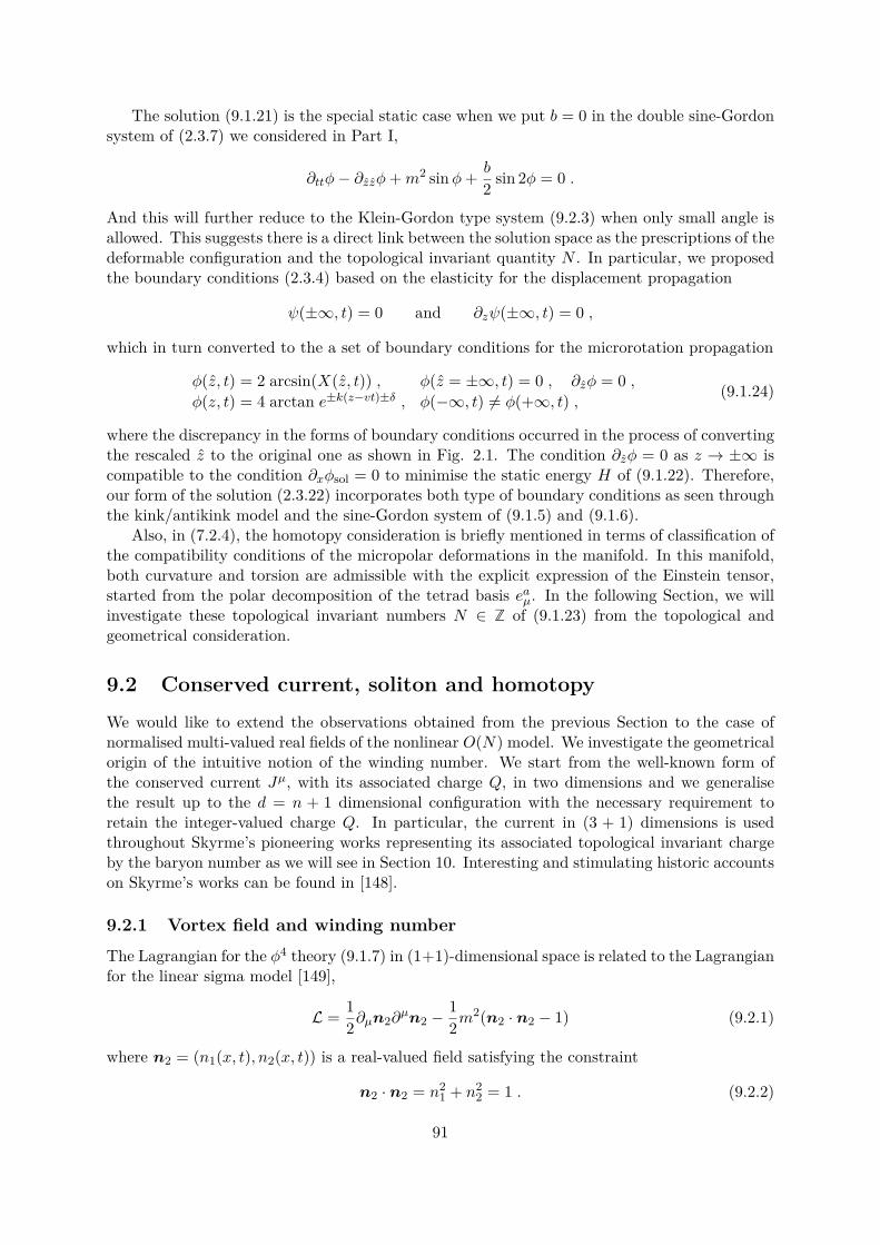
The solution (9.1.21) is the special static case when we put b = 0 in the double sine-Gordonsystem of (2.3.7) we considered in Part I,
∂ttϕ− ∂zzϕ+m2 sinϕ+ b
2 sin 2ϕ = 0 .
And this will further reduce to the Klein-Gordon type system (9.2.3) when only small angle isallowed. This suggests there is a direct link between the solution space as the prescriptions of thedeformable configuration and the topological invariant quantity N . In particular, we proposedthe boundary conditions (2.3.4) based on the elasticity for the displacement propagation
ψ(±∞, t) = 0 and ∂zψ(±∞, t) = 0 ,
which in turn converted to the a set of boundary conditions for the microrotation propagation
ϕ(z, t) = 2 arcsin(X(z, t)) , ϕ(z = ±∞, t) = 0 , ∂zϕ = 0 ,ϕ(z, t) = 4 arctan e±k(z−vt)±δ , ϕ(−∞, t) = ϕ(+∞, t) , (9.1.24)
where the discrepancy in the forms of boundary conditions occurred in the process of convertingthe rescaled z to the original one as shown in Fig. 2.1. The condition ∂zϕ = 0 as z → ±∞ iscompatible to the condition ∂xϕsol = 0 to minimise the static energy H of (9.1.22). Therefore,our form of the solution (2.3.22) incorporates both type of boundary conditions as seen throughthe kink/antikink model and the sine-Gordon system of (9.1.5) and (9.1.6).
Also, in (7.2.4), the homotopy consideration is briefly mentioned in terms of classification ofthe compatibility conditions of the micropolar deformations in the manifold. In this manifold,both curvature and torsion are admissible with the explicit expression of the Einstein tensor,started from the polar decomposition of the tetrad basis ea
µ. In the following Section, we willinvestigate these topological invariant numbers N ∈ Z of (9.1.23) from the topological andgeometrical consideration.
9.2 Conserved current, soliton and homotopyWe would like to extend the observations obtained from the previous Section to the case ofnormalised multi-valued real fields of the nonlinear O(N) model. We investigate the geometricalorigin of the intuitive notion of the winding number. We start from the well-known form ofthe conserved current Jµ, with its associated charge Q, in two dimensions and we generalisethe result up to the d = n + 1 dimensional configuration with the necessary requirement toretain the integer-valued charge Q. In particular, the current in (3 + 1) dimensions is usedthroughout Skyrme’s pioneering works representing its associated topological invariant chargeby the baryon number as we will see in Section 10. Interesting and stimulating historic accountson Skyrme’s works can be found in [148].
9.2.1 Vortex field and winding number
The Lagrangian for the ϕ4 theory (9.1.7) in (1+1)-dimensional space is related to the Lagrangianfor the linear sigma model [149],
L = 12∂µn2∂
µn2 − 12m
2(n2 · n2 − 1) (9.2.1)
where n2 = (n1(x, t), n2(x, t)) is a real-valued field satisfying the constraint
n2 · n2 = n21 + n2
2 = 1 . (9.2.2)
91
Here, the term m2 in (9.2.1) can be regarded as the Lagrangian multiplier. This system isinvariant under the global rotation SO(2), and the associated equation of motion is the Klein-Gordon equation,
(∂µ∂µ +m2)n2 = 0 . (9.2.3)
The constraint (9.2.2) implies that the field n2 resides on S1, and we can assign a new degreeof freedom, using the polar coordinate system, ϕ = ϕ(x, t) to write
n2(ϕ) = (cosNϕ, sinNϕ) . (9.2.4)
Now, there exists a conserved current (we will see more details of the origin of this currentlater)
Jµ = 12πϵ
µνϵabna∂νnb (9.2.5)
where µ, ν are the spacetime indices, and a, b = 1, 2 for the components of n2 = (n1, n2)describing the internal degrees of freedom. This current is again conserved quantity by itsconstruction,
∂µJµ ∝ ∂(n1, n2)
∂(t, x) . (9.2.6)
The quantity ∂µJµ is proportional to the Jacobian matrix, recognised as the determinant
of ∂µna, between the set of spacetime variables and the newly generated coordinates n2 =(cosNϕ, sinNϕ) under the constraint n2 · n2 = 1, hence it vanishes. In this case, the homotopygroup is
π1(S1) ∼= Z . (9.2.7)
The associated conserved total charge is then obtained by the integration
Q =∫ +∞
−∞J t dx = N
2π
∫ +∞
−∞
∂ϕ
∂xdx = N
2π [ϕ(+∞, t) − ϕ(−∞, t)] . (9.2.8)
Now, if we impose the asymptotic condition n2(±∞, t) approaches some finite values, as we didin evaluating the charge Q in (9.1.17), then we can assign the angular variable ϕ(x, t) to satisfythe condition
ϕ(+∞, t) = ϕ(−∞, t) + 2π . (9.2.9)
This gives the identification that the total charge is nothing but the integer N ∈ Z,
Q = N . (9.2.10)
Since the classification of the solution space is characterised by the homotopy consideration(9.2.7), this identification gives a direct link between the topological invariants and the numberof equivalent solution classification, as we will see more details in the next Section.
Geometrically, the nature of the invariant number N ∈ Z, we call it the winding numberwithout loss of generality henceforth, can be understood from the differential point of view fora two-dimensional static field in polar coordinates,
n2(ϕ) = (cosϕ, sinϕ) , (9.2.11)
where ϕ is a now time-independent function, ϕ(x, y) = arctan y/x. Now, we can write
dϕ = ∂ϕ
∂ydy + ∂ϕ
∂xdx = 1
r2 (xdy − ydx) , (9.2.12)
92

where r2 = x2 + y2. Then the identical integer N can be obtained in the static two-dimensionalcase from the purely geometric interpretation that N is the integration of the total changes inthe angular variable ϕ along the simple closed contour C divided by 2π, which is the genuineand intuitive notion of the counting the winding number,
N = 12π
∮Cdϕ = 1
2π
∮C
1r2 (xdy − ydx) . (9.2.13)
As shown in the above discussion, if we consider the spatial two-dimensional static config-uration, we would have the same topological invariant N in the geometrical static space withthe same homotopy group of the (1 + 1)-kink, but now S0 is changed to S1, on account of thetwo-dimensional spatial space (9.2.11). Therefore, the homotopy is a map from S1 to S1 so that
π1(S1) ∼= Z . (9.2.14)
For the field configuration in static case which yields the integerN under the identical constraint,we used n2 ·n2 = 1, the natural candidate for this purpose would be the two-dimensional vortexfield nv with an integer number N ,
nv = (cos(Nϕ), sin(Nϕ)) . (9.2.15)
The form of the conserved current (9.2.5) is still valid with the indices are now µ, ν = x, y.Then in terms of its angular variable ϕ(x, y), this is explicitly
Jµ = N
2πr r , (9.2.16)
where r = (x, y)/√x2 + y2 and r2 = x2 + y2. Now, a question arises. In the static vortex con-
figuration, how one can evaluate the total charge Q =∫
all space Jt without the time component
of the current? The answer comes from the purely geometrical consideration of (9.2.13) wherewe can write the component of the current in terms of spatial derivatives of the angular variableϕ. With the help of Green’s theorem, we can rewrite (9.2.13) by
N =∫
R∇ · J dxdy (9.2.17)
where R is the region surrounded by the closed contour C. But we note that the integrand isthe expression of the conserved current ∂µJ
µ = ∇ · J = 0. The clue for this problem comesfrom the fact that the form of the current (9.2.16) is not defined in the origin, but elsewhere.Hence, it will lead to the conclusion that it is the Dirac delta function in two dimensions [150]
∇ · J = N
2π∇ · r
r= N
2πδ2(r) . (9.2.18)
The configuration of (9.2.11) is a trivial case of N = 1, and any other vortex (or antivortexwith negative integers) configuration with the same topological number N can be obtained bysmooth deformations from the vortex field configuration (9.2.15) ensured by the topologicalinvariant total charge Q = N , hence belongs to the equivalent solution space.
Now, in order to understand the geometrical meaning of the winding number N better,we would like to consider a physical system of nematic liquid crystals of Section 8.3. In thissystem, the optical apparatus, such as two layers of mutually orthogonal polarisers, gives acharacteristic feature of the defects in its directors nN of (8.4.36) in the planar case formed bypatterns called brushes, also known as the Schlieren texture [124]. Since we can distinguish four
93
Figure 9.2: The four patterns we can count around a given point are shown in red boxes which arefiltered by double-layered polarisers on the model of planar nematic liquid crystals also shown as thevector field.
patterns through double-layered polarisers, we can trace the pattern around the given loop ofthe planar rotation to count the number of patterns, see Fig. 9.2.
For example, if we count four distinct patterns around the point of interest, this means wecan assign a unity to classify the defect occurred around that particular point. This physicalmeasure imposes some difficulties especially if one counts the pattern far away from the defectregion which might give different counts around the given loop.
From the mathematical point of view, this counting of the pattern is identical to the windingnumber defined by (9.2.13), and it is also closely related to the Frank’s vector F as the measureof disclination we introduced in terms of the Einstein tensor (7.1.12b)∮
C
12
ω ab
µ ϵ cab dxµ =
∫S
12
Rab
µνϵc
ab dxµ ∧ dxν =∫
S−
Gσcϵσµν dx
µ ∧ dxν = F c , (9.2.19)
where ω ab
µ is the metric compatible spin connection (6.1.2) satisfying ω ab
µ = − ω ba
µ . In partic-ular, if the defect in the nematic liquid crystals is governed by a fixed uniaxial vector ni with aplanar rotational angle ϕ, from (8.4.14) and (8.4.17) we can write
niϕ = −12ϵijkϕ ajk = −1
2ϵijkAjk (9.2.20)
where aij and Aij are antisymmetric 3 × 3 matrices in the exponential representation R = eA
of R ∈ SO(3). Then we have, around a simple closed loop C in the plane,∮Cd(niϕ) = ni
∮Cdϕ = −ni
∮C
12ϵijkdAjk = ni2πN. (9.2.21)
The integer N comes from the vortex field configuration (9.2.15) with the geometrical definitionof the winding number in the form of (9.2.13).
Furthermore, if we assign ∂µAjk = −
ω jkµ into (9.2.19) provided Ajk is smooth, we obtain
ni
∮Cdϕ = −ni
∮C
12ϵijk∂µA
jk dxµ = ni2πN = Fi . (9.2.22)
Therefore, the integer N gives us the notion of the winding number at least three differentoccasions, i) the geometrical integration, ii) the vortex field, iii) the number appears in theFrank’s vector as the measure of disclination in this case. Of course, in principle we might havehalf integers in the vortex field but we would like to restrict ourselves to the integer N . Thereason for this becomes apparent when we consider the conserved integer Q in Section 10.
As shown in Fig. 9.3, we can simulate the winding number contribution entirely comes fromthe vortex field configuration (9.2.15). In particular, in the case of N = 1, we can read off fourdistinct patterns around the centre which gives the winding number one by definition.
94

N = −1 N = 1 N = 2 N = 3
Figure 9.3: Vortex field configurations with various integers N solely using (9.2.15) are shown with thecomputer generated corresponding defects in the directors.
9.2.2 Conserved current in higher dimensions
We can extend our discussion to the field configuration n3 = (n1, n2, n3) satisfying n3 · n3 = 1in three dimensions, now n3 is on S2. The current in three dimensions is given by
Jµ = 18πϵ
µνρϵabcna∂νnb∂ρnc (9.2.23)
where µ, ν, ρ are spacetime indices in (2 + 1) dimensions and a, b, c = 1, 2, 3 are for the compo-nents indices of n3 = n3i. This current is again conserved and its divergence is proportional tothe Jacobian matrix similar to (9.2.6). We can compute the J t component which will give thetotal charge Q when we integrate it over all space,
J t = 14πn3 ·
(∂n3∂x
× ∂n3∂y
). (9.2.24)
This can be viewed as the volume element of a parallelepiped spanned by n3, ∂xn3, ∂yn3.This form of the current is related to the so-called Mermin-Ho relation [151] expressing the curlof the velocity in the form of the current (9.2.23) when one considers the director field of the Aphase of superfluid helium 3He.
Next, we would like to find an expression for the field configuration in three dimensions,which imposes the winding number N in a natural way, and satisfy the constraint n3 · n3 = 1.One such an expression comes from the idea that we might regard the non-trivial vortex fieldnv of (9.2.15) as a projection from the higher dimensional vortex field. This suggests we cansimply introduce an additional component in the higher dimensional configuration [152] whilewe can retain the constraint n3 · n3 = 1.
This can be done if we combine the non-trivial vortex field nv into the first two componentof n3, in such a way that
n3 = (sin θnv, cos θ)= (sin θ cosNϕ, sin θ sinNϕ, cos θ) .
(9.2.25)
The topological density (another name for the J t component) for this general field configurationcan be obtained simply inserting n3 into (9.2.24)
J t = 14π det
(n3,
∂n3∂x
,∂n3∂y
)= −N
4π sin θ ∂(ϕ, θ)∂(x, y)
= N
4πrθ′ sin θ ,
(9.2.26)
95
where θ′ = ∂θ/∂r, r2 = x2 + y2, and the Jacobian matrix of coordinate changes between thespherical and the Cartesian coordinate system is
−N sin θ = ∂(n1, n2, n3)∂(ρ, ϕ, θ) . (9.2.27)
Then, the conserved topological charge can be obtained from the integration,
Q =∫dxdy J t
= N
2 [cos f(0) − cos f(∞)] .(9.2.28)
If we set the radial function to satisfy, cos θ(0) − cos θ(∞) = 2 or equivalently θ(0) − θ(∞) = π,we obtain
Q = N . (9.2.29)The homotopy group in this case is a map from S2
phy to S2int, hence
π2(S2) ∼= Z . (9.2.30)
For the pure spatial three-dimensional field configuration n3 = (n1, n2, n3), we can considerthe field introduced by Polyakov [153], the hedgehog field nh lies on S2, see Fig. 9.4
nh = 1r
(x, y, z), r2 = x2 + y2 + z2 , (9.2.31)
corresponding to the N = 1 case of the trivial configuration n3 = (sin θ cosϕ, sin θ sinϕ, cos θ),and we will see more of this in Section 9.4.
We can calculate the associated total charge Q, using the divergence theorem to obtain∫dxdydz ∂µJ
µ =∫dSµJ
µ
= 18π
∫dSµϵ
µνρϵabcna∂νnb∂ρnc
= 14π
∫dS n3 ·
(∂n3∂x
× ∂n3∂y
).
(9.2.32)
In three dimensions the area of S2 sphere is 4π. This factor exactly cancels out the factor1/4π. Therefore, the topological density indeed agrees with (9.2.24). And we see that wewill obtain the identical total charge Q regardless we integrate J t from the time-dependentfield configuration in (n+ 1) dimensions over n spatial dimensions, or we integrate the spatialcomponents J from the static field configuration over (n + 1) purely spatial total space usingthe divergence theorem. The latter will give the direct notion of the topological invariant asthe degree of mapping of the surface S2 surrounding the defects on the sphere where the fieldn3 with the information of winding number N is embedded under the constraint n3 · n3 = 1to yield the homotopy (9.2.30).
Our next task is to construct a field configuration n4 satisfying n4·n4 = 1 in four dimensions.This can be done by writing, from our experience of (9.2.25)
n4 =(sinω(r)n3, cosω(r)
)(9.2.33)
where n3 is defined by (9.2.25) with the integer N firmly embedded. The conserved current,also known as Skyrme’s current, is
Jµ = 112π2 ϵ
µνλρϵabcdna∂νnb∂λnc∂ρnd . (9.2.34)
96

nv(N = 1) n3(N = 1) nv(N = 2) n3(N = 2)
Figure 9.4: Two-dimensional vortex field configurations with various integers N using (9.2.15) and itscorresponding n3 fields on S2 of (9.2.25) are shown where n3(N = 1) is essentially the isotropic directordistribution of hedgehog configuration nh.
One can compute the topological density by inserting (9.2.33) into (9.2.34)
J t = N
2π2 sin θ sin2 ω(r) ∂(ϕ, θ, ω(r))∂(x, y, z)
= − N
2π2ω′(r)r2 sin2 ω(r) ,
(9.2.35)
where we used the Jacobian matrix, similar to that of (9.2.27)
N sin θ sin2 ω(r) = ∂(n1, n2, n3, n4)∂(ρ, ϕ, θ, ω(r)) . (9.2.36)
The associated total charge can be obtained
Q = N
π[ω(0) − ω(∞)] − N
2π [sin 2ω(0) − sin 2ω(∞)] . (9.2.37)
Now, we notice that the second term on the right-hand side of (9.2.36) may impose thecondition against the consideration we discussed in terms of the finite energy requirement. Butif we write
sin 2ω(0) − sin 2ω(∞) = 2[sinω(0) cosω(0) − sinω(∞) cosω(∞)
],
then we can choose the arbitrary radial function ω(r) in such a way that it removes the possiblesingularity by putting sinω(0) = sinω(∞) = 0. Consequently, the function ω(r) removes thedivergence in the energy when r → ∞. Under these conditions, the problematic terms vanishand the total charge becomes
Q = N
π[ω(0) − ω(∞)] . (9.2.38)
In order to ensure the finite integer-valued Q, we further use the identity
sinA− sinB = 2 sin(A−B
2
)cos
(A+B
2
),
so that the condition sinω(0) = sinω(∞) = 0 implies that the identical asymptotic conditionon the radial function when we derived (9.2.29), ω(0) − ω(∞) = π. Therefore, the total chargebecomes
Q = N , (9.2.39)
97
as expected, and the homotopy group in this case is a map from S3phy to S3
int so that
π3(S3) ∼= Z . (9.2.40)
In deriving the expressions Q = N in (9.2.29) and (9.2.39), we can obtain the identicalresults but with an additional minus sign. To see this, as noted in [154], let us bring back thestereographic projection space we considered in Section 8.1. The vortex field travels from thesouth pole to the north pole, or it can travel in the reverse direction on S2 (or on S3), as rincreases from the origin to infinity on the projective plane or in the reverse order. Then, thetotal charge Q may acquire a minus sign depending on the choice of the path between the poles,hence Q = ±N . The factor that determines the sign is sometimes called the polarity.
Lastly, we would like to consider the mechanism that lies beneath in evaluating the inte-grations in various dimensions to assure the integer-valued Q in accordance with the homotopyclassification πn(Sn) ∼= Z. In general d dimensions, the form of the integration for the chargeQ would be ∫
ddx ∂µJµ =
∫dSµJ
µ . (9.2.41)
We can regard the term dSµ on the right-hand side as an infinitesimal surface element of thehypersurface Sd−1 embedded by the volume element ddx of the integration in d dimensions,defined on the left-hand side in the direction of the current Jµ. To see this, for the Euclideanlength element x, defined by the strictly positive-definite Euclidean metric tensor, the arbitraryvolume element in d dimensions ddx can be written by
ddx = dΩd dx xd−1 (9.2.42)
where∫dΩd is the area of a unit n-sphere Sn in d = n + 1 dimensions. This technique is
commonly used when one considers the dimensional regularisation in quantum field theory toremove the possible divergences in evaluating the integration [155]. Therefore, we can constructa conserved current in the general d dimensions
Jµ = 1n!∫dΩd
ϵµµ1···µnϵaa1···anna∂µ1na1 · · · ∂µnnan , (9.2.43)
where the factor n! comes from the number of permutations in the indices, and the explicitevaluation of
∫dΩd will be given shortly. This will give the topological invariant Q by the
integration (9.2.41) with the factor∫dΩd will be canceled out exactly in the integration. In
particular, when one considers a static d dimensional problem, the conserved current will takethe form
Jµ = N∫dΩd
r
rd−1 , r = (x1, · · · , xd) (9.2.44)
which yields the d-dimensional Dirac delta function,
∂µJµ = N∫
dΩd
(∫dΩd
)δd(r) . (9.2.45)
The corresponding field configuration in d dimensions is
nd = (sinωd(r)nd−1, cosωd(r)) , n2 = nv , d ≥ 3 (9.2.46)
with some angular functions ωd(r), satisfying nd · nd = 1 in d = n+ 1. The mapping betweenthe field configuration on the sphere Sn
phy and the sphere Snint in the integration (9.2.41) gives
precisely the homotopy classification we observed in (9.2.14), (9.2.30) and (9.2.40)
πn(Sn) ∼= Z . (9.2.47)
98
Nonetheless, the field configuration (9.2.46) is not unique for the purpose of obtaining thetopological invariants N . In [156] various forms of Jµ are given, for example, by noting thesimilarities from the sine-Gordon system which gives a set of distinct Q sectors. Notably,in [157], the form of field configuration n3 is given using an equality based on the lower boundfor the finite-energy consideration
∂µn3 = ±ϵµν (n3 × ∂νn3) . (9.2.48)
This further yields a conclusion that when the field configuration n3 is projected on the complexplane to form the analytic complex function w = w1 + iw2, then any such analytic functionwill give the topological invariants when one writes w in the power expansion of order N . Thesolution space itself imposes the scale invariance and the translational invariance.
The expression (9.2.42) can be illustrated in simple cases for d = 2 and d = 3, where theinfinitesimal elements to be integrated are expressed as the product of its differential angularelements and radial elements in the polar coordinate system, for example
d = 2 : dxdy = (dθ)(rdr) ,d = 3 : dxdydz = (sin θdθdϕ)(r2dr) .
The factor∫dΩd in general case is given by
∫dΩd = 2π d
2
Γ(
d2
) . (9.2.49)
Using the properties of Gamma function,
Γ(n+ 1) = nΓ(n), and Γ(1
2 + n
)= (2n)!
4nn!√π ,
we can summarise some special cases that frequently appears, as below.
Dimension d 1 2 3 4∫dΩd 2 2π 4π 2π2 (9.2.50)
9.3 Topological sectors
In the previous Sections, we started from the conserved current Jµ a priori to derive the con-served charge Q in the simple (1 + 1) dimensions up to the general case of (9.2.43). Unlike theconventionally derived conserved current such as Noether’s current, the topological invariantswe considered are entirely dependent on the asymptotic boundary conditions, and its conservedinvariant property comes from the finite energy requirement from the expression
Q ∝ ϕ(+∞, t) − ϕ(−∞, t) .
And we saw explicit field configurations for the associated conserved current in various dimen-sions, leading to the topological invariants
Q = N .
It becomes evident that our true starting point in developing the argument should be the finiteenergy requirement rather than the seemingly ad hoc construction of the currents Jµ. This
99
statement can be rephrased that the solution space ϕ should satisfy some finite-valued asymp-totic conditions. In this Section, we would like to justify the relation between the topologicallyinvariant total charge and the homotopy classification using a simple case.
Let us start again with the system of a single scalar field ϕ(x, t) in two dimensions. Wewrite the Lagrangian by
L = 12∂µϕ∂
µϕ− U(ϕ) , (9.3.1)
where the potential U(ϕ) might have an integer number of degenerate minima. In particular,the sine-Gordon system of (9.1.18) imposes the infinite number of minima of the system, withthe potential U(ϕ) = m2(1 − cosϕ) due to the periodicity in the solution space with the integerN .
If the system possesses a set of degenerate minima, the field (static or time-dependent)must approach a minimum of U(ϕ) at every point on spatial infinity for a given t, to retain itsfinite energy requirement. In this case, as we already imposed in (9.1.5) and (9.1.6), we defineformally such asymptotic conditions by
ϕ(+∞, t) = limx→+∞
ϕ(x, t) ≡ ϕ+∞ , ϕ(−∞, t) = limx→−∞
ϕ(x, t) ≡ ϕ−∞ . (9.3.2)
And there are two possibilities that either ϕ+∞ = ϕ−∞ or ϕ+∞ = ϕ−∞ within the finite energyrequirement. Then, the field ϕ(x, t) will change continuously as the time t varies and the solutionspace itself is derived from the equation of motion
∂µ∂µϕ = −∂U
∂ϕ. (9.3.3)
The trivial solution for this differential equation is again constant vacuum solution ϕvac, and ifnot, it will be a description of the continuous deformation of the system as we saw in Part I.Therefore, in a sense, the non-trivial solution can be regarded as a fluctuation ϕf of the vacuumsolution restricted by a finite-energy requirement
ϕ = ϕvac + ϕf (9.3.4)
belongs to each homotopy classification of the solution space, with the asymptotic behaviourthat ϕ → ϕvac as seen in the ϕ4 theory and the sine-Gordon system in Section 9.1.
The continuously deformable condition and the smoothness of the function ϕ suggests thatwe cannot expect the transition in the configuration of the system have an abrupt change fromϕ−∞ to ϕ+∞. Hence the transition within the given minima must occur smoothly in such away that the points of minima remain as the stationary points of U(ϕ) within the given classof solution space.
Therefore, there exist a number of regions called sectors [40] in the solution space in whichthe system is allowed to deform continuously around the point of minima while the finite energyrequirement is maintained. The sectors are topologically disconnected regions in the solutionspace, in a sense that fields configuration from one sector cannot be deformed continuously intoanother without violating the finite energy requirement. But the field configuration in any givensector stays within that sector as time changes.
Hence, this classification of sectors is closely related to the equivalent homotopy classificationof the solution space. This is an analogous analysis we made in (7.2.4) in Section 7.2. Inparticular, if there is only one unique minima, we have only one sector for the solution spaceand this corresponds to the case of ϕ(+∞, t) = ϕ(−∞, t) which is equivalent to the trivialcase Q = 0. This is the class 0 ∈ π1(SO(3)) we considered in (7.2.4), the equivalent set ofconfiguration that can be continuously deformed uniformly via diffeomorphism.
100
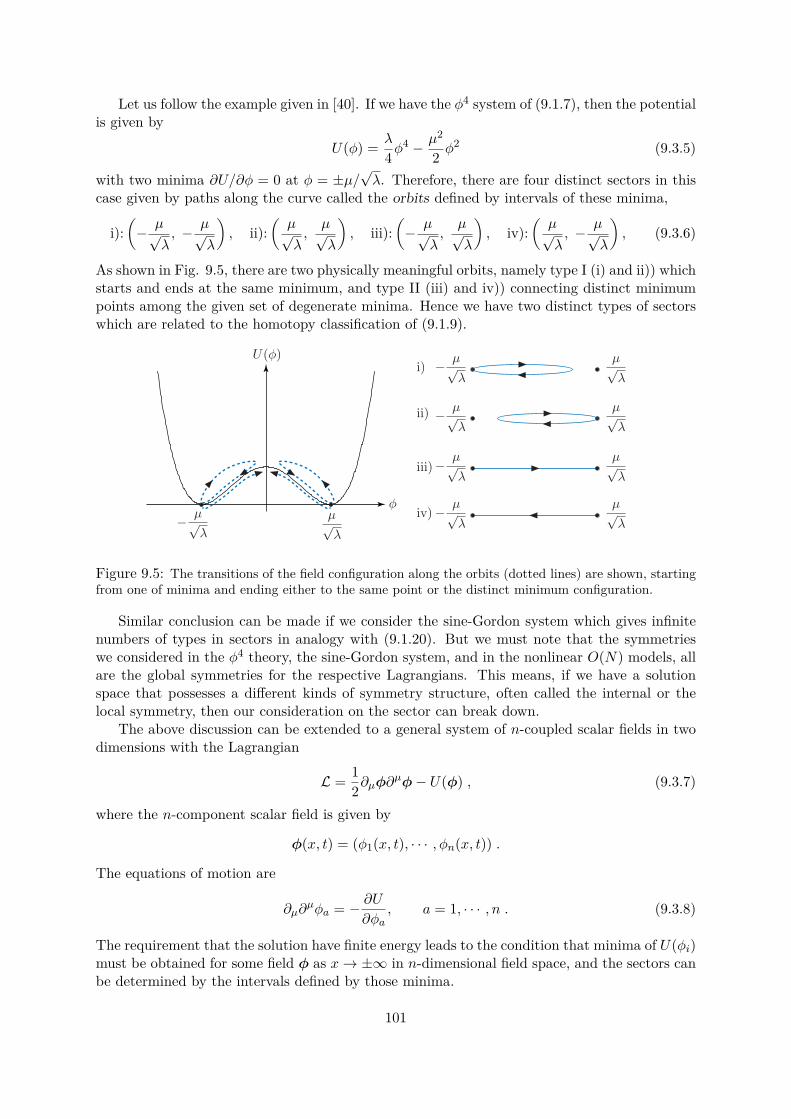
Let us follow the example given in [40]. If we have the ϕ4 system of (9.1.7), then the potentialis given by
U(ϕ) = λ
4ϕ4 − µ2
2 ϕ2 (9.3.5)
with two minima ∂U/∂ϕ = 0 at ϕ = ±µ/√λ. Therefore, there are four distinct sectors in this
case given by paths along the curve called the orbits defined by intervals of these minima,
i):(
− µ√λ, − µ√
λ
), ii):
(µ√λ,µ√λ
), iii):
(− µ√
λ,µ√λ
), iv):
(µ√λ, − µ√
λ
), (9.3.6)
As shown in Fig. 9.5, there are two physically meaningful orbits, namely type I (i) and ii)) whichstarts and ends at the same minimum, and type II (iii) and iv)) connecting distinct minimumpoints among the given set of degenerate minima. Hence we have two distinct types of sectorswhich are related to the homotopy classification of (9.1.9).
Figure 9.5: The transitions of the field configuration along the orbits (dotted lines) are shown, startingfrom one of minima and ending either to the same point or the distinct minimum configuration.
Similar conclusion can be made if we consider the sine-Gordon system which gives infinitenumbers of types in sectors in analogy with (9.1.20). But we must note that the symmetrieswe considered in the ϕ4 theory, the sine-Gordon system, and in the nonlinear O(N) models, allare the global symmetries for the respective Lagrangians. This means, if we have a solutionspace that possesses a different kinds of symmetry structure, often called the internal or thelocal symmetry, then our consideration on the sector can break down.
The above discussion can be extended to a general system of n-coupled scalar fields in twodimensions with the Lagrangian
L = 12∂µϕ∂µϕ − U(ϕ) , (9.3.7)
where the n-component scalar field is given by
ϕ(x, t) = (ϕ1(x, t), · · · , ϕn(x, t)) .
The equations of motion are
∂µ∂µϕa = − ∂U
∂ϕa, a = 1, · · · , n . (9.3.8)
The requirement that the solution have finite energy leads to the condition that minima of U(ϕi)must be obtained for some field ϕ as x → ±∞ in n-dimensional field space, and the sectors canbe determined by the intervals defined by those minima.
101
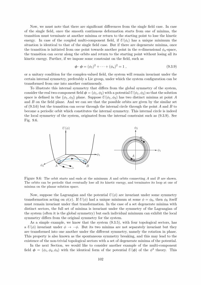
Now, we must note that there are significant differences from the single field case. In caseof the single field, once the smooth continuous deformation starts from one of minima, thetransition must terminate at another minima or return to the starting point to lose the kineticenergy. In case of the coupled multi-component field, if U(ϕi) has a unique minimum thesituation is identical to that of the single field case. But if there are degenerate minima, oncethe transition is initiated from one point towards another point in the n-dimensional ϕa-space,the transition can occur along the orbits and return to the starting point without losing all itskinetic energy. Further, if we impose some constraint on the field, such as
ϕ · ϕ = (ϕ1)2 + · · · + (ϕn)2 = 1 , (9.3.9)
or a unitary condition for the complex-valued field, the system will remain invariant under thecertain internal symmetry, preferably a Lie group, under which the system configuration can betransformed from one into another continuously.
To illustrate this internal symmetry that differs from the global symmetry of the system,consider the real two-component field ϕ = (ϕ1, ϕ2) with a potential U(ϕ1, ϕ2) so that the solutionspace is defined in the ϕ1, ϕ2 plane. Suppose U(ϕ1, ϕ2) has two distinct minima at point Aand B on the field plane. And we can see that the possible orbits are given by the similar setof (9.3.6) but the transition can occur through the internal circle through the point A and B tobecome a periodic orbit which constitutes the internal symmetry. This internal circle is indeedthe local symmetry of the system, originated from the internal constraint such as (9.3.9). SeeFig. 9.6.
Figure 9.6: The orbit starts and ends at the minimum A and orbits connecting A and B are shown.The orbits can be periodic that eventually lose all its kinetic energy, and terminates its loop at one ofminima on the planar solution space.
Now, suppose the Lagrangian and the potential U(ϕ) are invariant under some symmetrytransformation acting on ϕ(x). If U(ϕ) had a unique minimum at some ϕ = ϕ0, then ϕ0 itselfmust remain invariant under that transformation. In the case of a set degenerate minima withdistinct sectors, the full set of minima is invariant under the symmetry of the Lagrangian ofthe system (often it is the global symmetry) but each individual minimum can exhibit the localsymmetry differs from the original symmetry for the system.
As a simple example, we know that the system (9.3.5), with four topological sectors, hasa U(ϕ) invariant under ϕ → −ϕ. But its two minima are not separately invariant but theyare transformed into one another under the different symmetry, namely the rotation in phase.This property is also known as the spontaneous symmetry breaking, and this may lead to theexistence of the non-trivial topological sectors with a set of degenerate minima of the potential.
In the next Section, we would like to consider another example of the multi-componentfield ϕ = (ϕ1, ϕ2, ϕ3) with the identical form of the potential U(ϕ) of the ϕ4 theory. This
102
configuration is known as the Polyakov’s hedgehog field with the solution nh we saw in (9.2.31).
9.4 Polyakov’s hedgehog fieldIn 1974, Polyakov showed [153] that under the weak interaction assumption, the finite range ofmass spectrum can be obtained from the Hamiltonian H following the finite energy requirementof the system with the Lagrangian of the higher dimensional ϕ4 theory in (1 + 1) dimensionswe considered in (9.1.7). For (3 + 1) dimensions, the Lagrangian is given by
L = 12∂µϕ∂µϕ − U(ϕ) , (9.4.1)
whereU(ϕ) = −µ2
2 ϕ2 + λ
4 ϕ4 , (9.4.2)
for the three-component field ϕ = (ϕ1, ϕ2, ϕ3). The equation of motion identical to (9.3.8), isgiven by
∂µ∂µϕa −
(µ2 − λ(ϕ · ϕ)
)ϕa = 0 . (9.4.3)
A solution for the static case is given by
ϕa = nhaΘ(r), nha = 1r
(x, y, z) (9.4.4)
where r2 = x2 + y2 + z2 and nh = nha for a = 1, 2, 3 is the field configuration of (9.2.31). Anangular function Θ(r) satisfies the second-order ordinary differential equation
Θ′′ + 2r
Θ′ +(µ2 − 2
r2
)Θ − λΘ3 = 0 . (9.4.5)
Apart from the trivial vacuum solutions, i.e. the zeros of the potential U(ϕ), the non-trivialsolution must impose the asymptotic condition that approaches the vacuum solution
Θ(r → ∞) = µ√λ, (9.4.6)
The solution (9.4.4) is called the hedgehog solution, as we can see that these are isovectorsdirected along the radial vector at a given point.
For the rank-two tensor field, also known as the isotensor Higgs field, it is suggested byPolyakov that the solution shall be of the form
ϕab =(nhanhb − 1
3δab
)Θ(r) , a, b = 1, 2, 3 (9.4.7)
in place of ϕa in (9.4.4). We note that this is the identical form of the order parameter Q of(8.4.7) for the nematic liquid crystals we obtained in Section 8.4.
Qij =(nNinNj − 1
3δij
)σ , i, j = 1, 2, 3 . (9.4.8)
This enters into the energy density function F of (8.4.3) in the various forms of the invariant. Wenote that Θ(r) in (9.4.7) is a function of the position, but σ is a mere constant parameter. Thisimplies, unlike the space S2 where the nematic liquid crystals with directors nN are identifiedas the antipodals, we might need higher dimensional space with an additional degree of freedomto harbour the higher-ranked field configuration with some analogous notion of the antipodalidentification on that space. It is tempting to promote (9.4.7) to be the order parameter forthe micropolar continuum, in line of generalisation of nematic liquid crystals to the micropolarcontinuum in terms of director fields we saw in Section 8.4. This is the subject we would liketo investigate in the next Chapter, followed by formal justification.
103

104
Chapter 10
Micropolar continuum and theSkyrme model
A finite energy configuration requires appropriate asymptotic conditions in the total charge Q,for example in (9.2.28) and (9.2.38), to satisfy certain criteria as we observed in the previousSections with the currents Jµ in various dimensions. We would like to focus on the fieldconfiguration n itself constituting such currents Jµ in higher dimensions. This includes theSkyrme model as the spinor system in which the relation between SU(2) and SO(3) signifiesits role in various forms of the representation. This further will give us a unique point of viewto understand the result we obtained in Part II to connect the deformational measures we usedso far.
It is hinted in [35] that the order parameter for the micropolar continua can be taken asSO(3) or RP 3, and in [120] the elements of R ∈ SO(3) are briefly mentioned as the antipodalson S3. Using the fibrations between the unit spheres and the real projective space, we wouldlike to generalise the idea that micropolar continua can be regarded as the projective spacethat contains the nematic liquid crystals as its submanifold followed by the topological and ge-ometrical consideration. This approach is different from that of [142] promoting the micropolarcontinua as the general case of nematic liquid crystals.
10.1 Rotations of SO(3) and SU(2)An element R of the orthogonal rotation group SO(3), satisfying RTR = 1, can be expressedby the real 3 × 3 matrix representation we considered in (8.4.20), which is equivalent to (1.2.31)
Rij = cos Θ · δij + n3in3j(1 − cos Θ) − ϵijkn3k sin Θ . (10.1.1)
This describes the rotation of an angle Θ about the normalised axis
n3 = n3i satisfying n3 · n3 = 1 . (10.1.2)
where i, j, k = 1, 2, 3. We are particularly interested in the position-dependent axial configura-tion. For this purpose, we can choose the axis to be the hedgehog field nh of (9.2.31) or thegeneral field n3 of (9.2.25), which gives the topological invariant N in three dimensions. Inparticular, when N = 1, the hedgehog field is just the static n3 in the usual polar coordinatesystem
nh = (sin θ cosϕ, sin θ sinϕ, cos θ) , (10.1.3)
where ϕ = arctan(y/x) and θ = arctan(√x2 + y2/z).
105
An element U of the unitary rotational group SU(2), satisfying U †U = I, can be representedby a complex 2 × 2 matrix with two complex parameters a, b ∈ C
U =(a −bb a
)where |a|2 + |b|2 = 1 . (10.1.4)
Since there is a direct isomorphism of Cn ∼= R2n, we can assign a set of four real parameters(n1, n2, n3, n4) in such a way that a = n4 + in3 and b = −n2 + in1. Then (10.1.4) becomes
U =(n4 + in3 in1 + n2in1 − n2 n4 − in3
)= n4 · I + i(n · σ) , (10.1.5)
where n4 = (n, n4) = (n1, n2, n3, n4) satisfies the condition
n4 · n4 = 1 . (10.1.6)
We should not be confused with the first three components n of n4 and n3 ∈ S2 satisfyingn3 · n3 = 1 which enters into the representation of (10.1.1) as the normalised axis field in threedimensions. The Pauli matrices σ = (σ1, σ2, σ3) in (10.1.5) are the generators of SU(2), definedby
σ1 =(
0 11 0
), σ2 =
(0 −ii 0
), σ3 =
(1 00 −1
). (10.1.7)
It is sometimes convenient to write elements U ∈ SU(2) and R ∈ SO(3), respectively,
U = eiω(r)n3·σ and R = eiΘn3·J . (10.1.8)
The quantities ω(r) and Θ are the rotational angles about respective axes. Under these rep-resentations, the generators σ and J for SU(2) and SO(3), respectively, satisfy commutationrelations [
σi
2 ,σj
2
]= iϵijk
σk
2 and [Ji, Jj ] = iϵijkJk . (10.1.9)
Using the identity for the Pauli matrices,
σiσj = δij · I + iϵijkσk , (10.1.10)
we can show that (n3 · σ)2 = I. This implies that the even power of (n3 · σ) is I, and the oddpower becomes (n3 · σ). Hence, the form of the element U ∈ SU(2) is indeed,
eiω(r)n3·σ = cosω(r) · I + i(n3 · σ) sinω(r)= n4 · I + i(n · σ)
(10.1.11)
where we put n = n3 sinω(r) and n4 = cosω(r) for n3 · n3 = n4 · n4 = 1. This is precisely thefield configuration n4 of (9.2.33) we used in deriving the topological invariant N by Skyrme’scurrent Jµ of (9.2.34).
n4 =(sinω(r)n3, cosω(r)
). (10.1.12)
An explicit relation between R ∈ SO(3) and U ∈ SU(2) can be explained in many ways,but we would like to take a quaternion for the apparent topological benefit. A quaternion q isdefined by
q = a+ bi + cj + dk (10.1.13)
106
such that a, b, c, d ∈ R satisfy
a2 + b2 + c2 + d2 = 1 and i2 = j2 = k2 = −1 . (10.1.14)
So, it is easy to see that q lives on the sphere S3, and there is a direct isomorphism betweenU ∈ SU(2) of (10.1.5) and the representation of the quaternion. Explicitly, this is
q = a · I + (b, c, d) · (i, j,k) (10.1.15)
or equivalently, the isomorphism ofiσ ∼= (i, j,k) . (10.1.16)
In particular, if we have a pure imaginary quaternion there is a one-to-one correspondencebetween a quaternion and an element of R3 which transforms under the rotation SO(3). Thisallows us to take the Pauli matrices σ to transform under the rotation, regarding it as a three-component vector acted by the rotation in such a way that
σi = σjRji .
On the other hand, since each Hermitian matrix of the three-component σ transforms underU ∈ SU(2), we must have
σi −→ U †σiU .
Hence, as introduced in [158], the relation between U ∈ SU(2) and R ∈ SO(3) can be writtenby
σiRij = U †σjU . (10.1.17)
After applying σk on both sides, we take traces using the identity tr(σiσj) = 2δij which can beeasily seen from (10.1.10). Then (10.1.17 gives an explicit correspondence between U ∈ SU(2)and R ∈ SO(3), used in [159], by
Rij = 12tr
(σiU
†σjU), (10.1.18)
where the trace are taken over 2 × 2 matrices is understood if we write this in components
Rij = 12[σkl
(i)U†lt
]kt
[σtl
(j)Ulk
]tk. (10.1.19)
Since U and −U will give rise to the identical R, this confirms the two-to-one mapping betweenSU(2) and SO(3). Straightforward calculation of (10.1.19) by inserting the matrix elements ofU of (10.1.5) gives the representation of Rij in terms of (ni, n4) for i, j = 1, 2, 3
Rij = 2ninj − 2ϵijknkn4 + δij(2n24 − 1) (10.1.20)
in which, we used the constraint n2i + n2
4 = 1 of (10.1.6), and trace identities
trσi = 0, tr(σiσj) = 2δij , tr(σiσjσk) = 2iϵijk, tr(σiσjσsσt) = δijδst − δisδjt + δitδjs .
Therefore, we can confirm the well-known correspondence SU(2) −→ SO(3) stating that SU(2)is a double cover of SO(3)
SU(2)/−I, I ∼= SO(3) .
Moreover, if we putni = n3 sin Θ
2 and n4 = cos Θ2 , (10.1.21)
into (10.1.20), we will recover the previous representation (10.1.1).
107
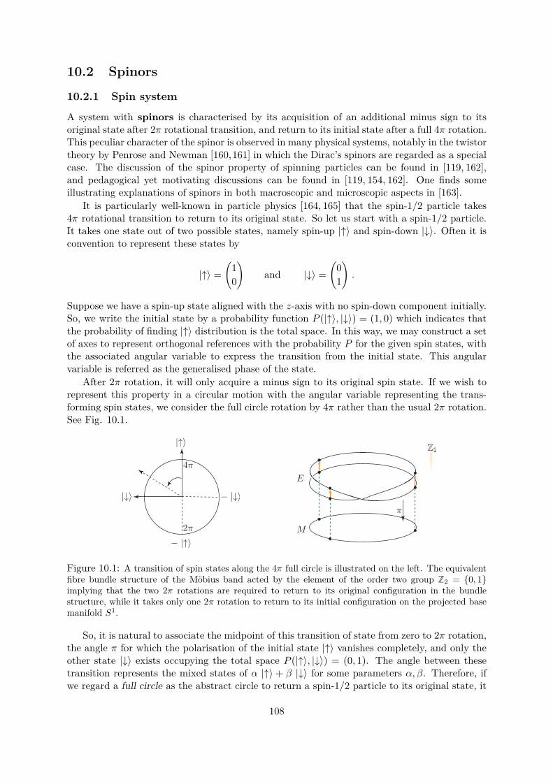
10.2 Spinors
10.2.1 Spin system
A system with spinors is characterised by its acquisition of an additional minus sign to itsoriginal state after 2π rotational transition, and return to its initial state after a full 4π rotation.This peculiar character of the spinor is observed in many physical systems, notably in the twistortheory by Penrose and Newman [160,161] in which the Dirac’s spinors are regarded as a specialcase. The discussion of the spinor property of spinning particles can be found in [119, 162],and pedagogical yet motivating discussions can be found in [119, 154, 162]. One finds someillustrating explanations of spinors in both macroscopic and microscopic aspects in [163].
It is particularly well-known in particle physics [164, 165] that the spin-1/2 particle takes4π rotational transition to return to its original state. So let us start with a spin-1/2 particle.It takes one state out of two possible states, namely spin-up |↑⟩ and spin-down |↓⟩. Often it isconvention to represent these states by
|↑⟩ =(
10
)and |↓⟩ =
(01
).
Suppose we have a spin-up state aligned with the z-axis with no spin-down component initially.So, we write the initial state by a probability function P (|↑⟩, |↓⟩) = (1, 0) which indicates thatthe probability of finding |↑⟩ distribution is the total space. In this way, we may construct a setof axes to represent orthogonal references with the probability P for the given spin states, withthe associated angular variable to express the transition from the initial state. This angularvariable is referred as the generalised phase of the state.
After 2π rotation, it will only acquire a minus sign to its original spin state. If we wish torepresent this property in a circular motion with the angular variable representing the trans-forming spin states, we consider the full circle rotation by 4π rather than the usual 2π rotation.See Fig. 10.1.
Figure 10.1: A transition of spin states along the 4π full circle is illustrated on the left. The equivalentfibre bundle structure of the Möbius band acted by the element of the order two group Z2 = 0, 1implying that the two 2π rotations are required to return to its original configuration in the bundlestructure, while it takes only one 2π rotation to return to its initial configuration on the projected basemanifold S1.
So, it is natural to associate the midpoint of this transition of state from zero to 2π rotation,the angle π for which the polarisation of the initial state |↑⟩ vanishes completely, and only theother state |↓⟩ exists occupying the total space P (|↑⟩, |↓⟩) = (0, 1). The angle between thesetransition represents the mixed states of α |↑⟩ + β |↓⟩ for some parameters α, β. Therefore, ifwe regard a full circle as the abstract circle to return a spin-1/2 particle to its original state, it
108
will take 4π rotation rather than the usual 2π rotation in the physical space.
Angle(phase): 0 π 2π 3π 4πState: |↑⟩ |↓⟩ − |↑⟩ − |↓⟩ |↑⟩
In Fig. 10.1, a fibre bundle structure S1, S1,Z2, π is shown describing the particle circlingon S1 becomes the opposite configuration from the original one after 2π rotation in the bundlespace. We can regard the bold lines in Fig. 10.1 as the edge of the Möbius band. It will taketwo such rotations to return to its original configuration. This structure is projected to the basemanifold S1 by a map π with the usual full circle of 2π rotation. Each dot on the base S1 willhave two distinct configurations when the group Z2 is acted on the fibre bundle. That means,we can associate 2π rotation an element 1 and 0 or 4π rotation an element 0.
10.2.2 Fibration in the projective space
Now, since we have the correspondences between SU(2) and SO(3), as we saw in the previousSection where each of these are isomorphic to the respective spaces,
SU(2) ∼= S3 and SO(3) ∼= S2 , (10.2.1)
what is left to do next is to establish the explicit relation between S3 and S2. Such a relationcan be understood by Hopf fibration of (8.1.10). In particular the fibration
S1 → S3 → S2 (10.2.2)
gives a unique identification CP 1 ∼= S2 via a fibration
S1 → S2n+1 → CPn . (10.2.3)
For the n = 1 case, we have an isomorphism in terms of the complex projective space
CP 1 ∼= S3/S1 ∼= S2 . (10.2.4)
To see this relation more closely, we note that a real-valued field x = (x1, · · · , x2n) ∈ R2n canbe translated into a complex-valued field z = (z1, · · · , zn) ∈ Cn by setting
z1 = x1 + ix2, z2 = x3 + ix4, · · · , zn = x2n−1 + ix2n .
In particular, if we impose a constraint x21 + · · · + x2
2n = 1 for the real-valued field, then thisfield configuration lies on S2n−1. For example, if n = 1 we only have z = x1 + ix2 such thatx2
1 +x22 = 1. This corresponds to a complex number z ∈ C with a modulus 1 on S1, i.e. |z| = 1.
If n = 2, we have
x = (x1, x2, x3, x4) ∈ S3 and z = (z1, z2) ∈ C2 .
So that we may define a complex doublet z ∈ C2 which lives on S3 as the doublet acted byU ∈ SU(2) of (10.1.5) on the state |↑⟩. For example
z =(z1z2
)= U |↑⟩ = U
(10
)=(n4 + in3
−n2 + in1
)(10.2.5)
satisfying n21 + n2
2 + n23 + n2
4 = 1, or equivalently |z1|2 + |z2|2 = 1. Similarly, we can define theaction of U ∈ SU(2) on the spin down state by ω = U |↓⟩.
109
These particular choice of states in (10.2.5) remove the redundancy in expressing the ele-ments of U ∈ SU(2) that comes from its unitary property U †U = I. This justifies the fieldconfiguration is indeed on S3 with the constraint (not to be confused with zz†, which is irrele-vant in this case)
z†z = 1 . (10.2.6)Hence, we can interpret the doublet z as the wavefunction of the spin-1/2 particle, and thisfield is invariant under the phase transformation,
z −→ eiαz . (10.2.7)
where eiα ∈ U(1) ∼= S1 as we noted in Fig. 10.1. In other words, the doublet z imposes aninternal symmetry U(1) in addition to the originally imposed symmetry on the space SU(2) ∼= S3
by the constraint n4 · n4 = 1. Hence, we can recognise the field configuration z on S3 must bein the complex projective space CP 1, by taking the quotient space with its internal symmetryU(1). Therefore, it is the fibration (10.2.4).
In case of the real projection space, the fibration is
S0(= Z2) → Sn → RPn , (10.2.8)
So that the corresponding quotient space is
RP 3 ∼= S3/Z2 (10.2.9)
in which we recognise Z2 the antipodals n,−n in the real space. Therefore, in the complexprojection space (10.2.4) the (complex)antipodals on S3 are taken to be S1. We also note thatthe antipodals in real and complex space are invariant under SO(2) and U(1) respectively,
Quotient space Antipodals Symmetry groupS3/S0 ∼= RP 3 : n,−n SO(2)S3/S1 ∼= CP 1 : z, eiαz U(1)
(10.2.10)
in which SO(2) and U(1) are related by the so-called σ-structure introduced by Trautman [109]explaining the appearance of the new gauge fields Aij and its associated gauge invariant fieldFij shown by Utiyama [71] in formulating the general local symmetry group SU(N).
10.2.3 Hopf map
The homotopy groups from the fibrations of the real and the complex projective space are givenby
π2(CP 1) ∼= π2(S3/S1) ∼= π2(S2) ∼= Z (10.2.11)and
π1(RP 3) ∼= π1(S3/S0) ∼= Z2 . (10.2.12)Now, the Hopf map H gives an explicit expression for the transformations from the field
z ∈ S3 into the axial field n3 ∈ S2 defined by
H : S3 −→ S2
H(z) −→ z†σz(10.2.13)
where σ are the Pauli matrices. One such coordinate representation of CP 1 is given by thedoublet z acted by U of (10.1.5), with its matrix entries are given by n4 of (10.1.12), on thestate |↑⟩,
z = U |↑⟩ = U
(10
)=(
cosω(r) + i cos θ sinω(r)ieiNϕ sin θ sinω(r)
). (10.2.14)
110
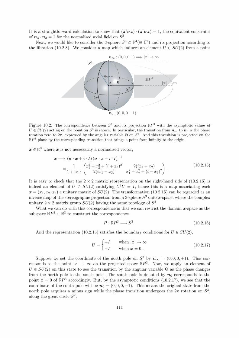
It is a straightforward calculation to show that (z†σz) · (z†σz) = 1, the equivalent constraintof n3 · n3 = 1 for the normalised axial field on S2.
Next, we would like to consider the 3-sphere S3 ⊂ R4(∼= C2) and its projection according tothe fibration (10.2.8). We consider a map which induces an element U ∈ SU(2) from a point
Figure 10.2: The correspondence between S3 and its projection RP 3 with the asymptotic values ofU ∈ SU(2) acting on the point on S3 is shown. In particular, the transition from n∞ to n0 is the phaserotation zero to 2π, expressed by the angular variable Θ on S3. And this transition is projected on theRP 3 plane by the corresponding transition that brings a point from infinity to the origin.
x ∈ R3 where x is not necessarily a normalised vector,
x −→ (σ · x + i · I) (σ · x − i · I)−1
= 11 + |x|2
(x2
1 + x22 + (i+ x3)2 2(ix1 + x2)
2(ix1 − x2) x21 + x2
2 + (i− x3)2
).
(10.2.15)
It is easy to check that the 2 × 2 matrix representation on the right-hand side of (10.2.15) isindeed an element of U ∈ SU(2) satisfying U †U = I, hence this is a map associating eachx = (x1, x2, x3) a unitary matrix of SU(2). The transformation (10.2.15) can be regarded as aninverse map of the stereographic projection from a 3-sphere S3 onto x-space, where the complexunitary 2 × 2 matrix group SU(2) having the same topology of S3.
What we can do with this correspondence is that we can restrict the domain x-space as thesubspace RP 3 ⊂ R3 to construct the correspondence
P : RP 3 −→ S3 . (10.2.16)
And the representation (10.2.15) satisfies the boundary conditions for U ∈ SU(2),
U =
+I when |x| → ∞−I when x = 0 .
(10.2.17)
Suppose we set the coordinate of the north pole on S3 by n∞ = (0, 0, 0,+1). This cor-responds to the point |x| → ∞ on the projected space RP 3. Now, we apply an element ofU ∈ SU(2) on this state to see the transition by the angular variable Θ as the phase changesfrom the north pole to the south pole. The south pole is denoted by n0 corresponds to thepoint x = 0 of RP 3 accordingly. But, by the asymptotic conditions (10.2.17), we see that thecoordinate of the south pole will be n0 = (0, 0, 0,−1). This means the original state from thenorth pole acquires a minus sign while the phase transition undergoes the 2π rotation on S3,along the great circle S2.
111
The presence of the factor 1/2 that appears in the field configuration for n4 of (10.1.21)may look a bit artificial at first sight, although it is required to recover the representationfor R ∈ SO(3) of (10.1.1) from the representation that does not contain any explicit angularexpression (10.1.20). But we now can see, for example through the coordinates for the northpole and the south pole on S3, it is absolutely required to validate the arguments we developedso far. A different approach in explaining for the origin of this half angle can be found in [114].
The north pole n∞ and the south pole n0 on S3 satisfy the following asymptotic conditions,while the transition of the element U ∈ SU(2) changes +I → −I as the phase changes from 0to 2π using (10.2.15),
Phase SU(2) S3 RP 3
0 +I n∞(0, 0, 0,+1) |x| → ∞2π −I n0 (0, 0, 0,−1) x = 0
(10.2.18)
For example, if we put a spin state |↑⟩ at the north pole n∞ on S3, this will be projected to|x| → ∞ on the RP 3 plane. If we bring this to the point x = 0 on the real projective plane, thecorresponding state will travel along the great circle on S3 marking the 2π rotation. In turn,this state will acquire additional minus sign. We summarise the transitions as follows.
n∞ : (0, 0, 0,+1) n0 : (0, 0, 0,−1)S3 : z = I |↑⟩ = +
(10)
−→ z′ = −I |↑⟩ = −(1
0)
RP 3 : |x| → ∞ −→ x = 0(10.2.19)
This establishes the direct link between the state lives on S3 acted by SU(2), and the statelives on RP 3 acted by SO(3). But what physical system shall we put on S3 and RP 3 actedupon by these rotations respectively? We would like take such a state on S3 as the Skyrmionand we will consider the possible candidate for the state living on the projective space RP 3 inthe following Sections.
10.3 SkyrmionsIn a series of papers [159, 166–169] Skyrme introduced a nonlinear field theory in describingstrongly interacting particles. This work has motivated many subsequent studies, and notedsome interesting links between baryon numbers (the sum of the proton and neutron numbers)and topological invariants in field theory.
Skyrme defined the field of complex doublet z ∈ C2 acted by an element of U ∈ SU(2)which lies on S3 [170–172], as we defined in (10.2.5) or (10.2.14)
z =(n4 + in3
−n2 + in1
), (10.3.1)
satisfying n21 + n2
2 + n23 + n2
4 = 1 which we know from the representation (10.1.5)
U = n4 · I + i(n · σ) .
The construction of this field comes from the fact that two distinct SO(3) transformationsact on the intrinsic elementary particle spin space and isospin space consists with a pion field(π0, π+, π−) independently. Then the property of SU(2) as the double cover of SO(3) is used tocontain the complex doublets z. Therefore, two independent full circles in each SO(3) for thespin-isospin coupled field means one 4π full circle in SU(2) ∼= S3. We note that the operatorin the isospin space has nothing to do with the physical spin space. But it acts on the three
112
states of pion field, and its generators I share the identical group structure with those of theusual generators J of SO(3), such as the commutation relation (10.1.9).
A fieldBaµ is defined as the gradient of pion field z, or equivalently the gradient of U ∈ SU(2)
on S3 by∂µU = iσaBa
µU (10.3.2)where a, b, c = 1, 2, 3 are for the isospin space, µ, ν, ρ for the (3 + 1)-dimensional spacetimeindices. We will use i, j, k = 1, 2, 3 for the spin space. Then using the identity tr(σaσb) = 2δab,one can obtain
Baµ = 1
2itr(U †σa∂µU
). (10.3.3)
Further, it can be shown that by inserting the representation for the rotation R ∈ SO(3) of(10.1.20),
Rab = 2nanb − 2ϵabcncn4 + δab(2n24 − 1)
directly into the definition of (10.3.3) using the relation (10.1.18), an equivalent expression ofBa
µ can be obtained by
Baµ = −1
4ϵabcRbd∂µRcd . (10.3.4)
Now, let us suppress the index notation for the coordinates µ, ν = 1, 2, 3 for now. Then we noticethat the term on right-hand side Rbd∂µRcd of (10.3.4) is precisely the form of the contortiontensor Kbµc of (6.2.3), when it is applied by global rotations Q ∈ SO(3) according to QTKQ.This gives the relation between Ba
µ field and Nye’s tensor (6.2.8) as follows.
Baµ = 1
2Γaµ . (10.3.5)
This relation between two fields gives us a unique identification in what we have discussedextensively in Part II, the compatibility conditions. A Maurer-Cartan form M = A−1dA, forA is an element of a Lie matrix group, M satisfies a Maurer-Cartan equation as we brieflymentioned in (6.2.12). Since Ba
µ is in the Maurer-Cartan form by definition, or iσB = U †dU ,it must satisfy the Maurer-Cartan equation
dB = −B ∧B , (10.3.6)
which can be equivalently written
∂µBaν − ∂νB
aµ + 2ϵabcB
bνB
cµ = 0 . (10.3.7)
After applying ϵνµσ, we obtainCurlB + 2Cof B = 0 .
Then, using the definition of the Cof of (4.2.2) and the relation (10.3.5), we recover our com-patibility condition for Nye’s tensor (6.2.9),
Curl Γ + Cof Γ = 0 . (10.3.8)
We recall that this is essentially derived from the setting (6.2.4) of vanishing curvature butnon-trivial torsion,
Rρσµν = ∂µK
ρνσ − ∂νK
ρµσ +Kρ
µλKλνσ −Kρ
νλKλµσ . (10.3.9)
Again this is in the form of the Maurer-Cartan equation, for the contortion tensor K = RTdRsatisfying
dK = −K ∧K . (10.3.10)
113
In [168], Skyrme used the explicit field configuration for (10.2.5) in terms of (10.1.21),
ni = n3 sin Θ2 and n4 = cos Θ
2 , (10.3.11)
but with n3 is given by the tetrad field eai-rotated hedgehog field
n3 = eainh satisfying n3 · n3 = 1 . (10.3.12)
In words, the field configuration n3 is obtained from the eai-transformed isotropic nh in the
spin-isospin system. Moreover, the constraint n3 · n3 = 1 immediately indicates that the tetradfield ea
i must be an orthogonal matrix, hence it can be regarded as the microrotation χaµ when
we use the polar decomposition (5.1.7) and (6.3.3). And when we insert (10.3.11) into (10.3.3),the explicit expression for Ba
i is obtained by
Bai = ea
j
12r[(δij − nhinhj) sin Θ + nhinhj rΘ′ − ϵijknhk(1 − cos Θ)
](10.3.13)
where B is now a strictly 3 × 3 matrix, representing the gradient of the spinor field, in termsof three position-dependent hedgehog fields under the constraint nh · nh = 1 and an arbitraryradial function Θ.
Skyrmions are field configurations for the quantised invariant number defined by the totalcharge of integration of the conserved current Jµ of (9.2.34) we saw in Section 9.2. Thistopological invariant number is regarded as a particle-like quantity, and postulated to be baryonnumber. In particular, under the configuration (10.3.11), one can obtain the topologicallyconserved charge Q = N = 1. In this case, one proton or one neutron. This is because the fieldconfiguration is expressed in terms of the hedgehog field nh, which does not contain any vortexfield but the trivial one N = 1, as we noticed in (9.2.31). In other words, if we use the generalspinor configuration such as (10.2.14), we will obtain a non-trivial baryon number N by theintegration
N = 112π2
∫d3x ϵtνλρϵabcdna∂νnb∂λnc∂ρnd
= − 12π2
∫d3x detB .
(10.3.14)
Using the relation with Nye’s tensor (10.3.5), this can be rewritten by
N = − 1(4π)2
∫d3x det Γ . (10.3.15)
Furthermore, after a rather lengthy calculation using the relation with the contortion tensor Kof (6.2.8), this becomes
N = 196π2
∫d3x tr (K ∧K ∧K) . (10.3.16)
All three expressions (10.3.14), (10.3.15) and (10.3.16) will give an identical topological invariantinteger N , satisfying the finite energy requirement we considered in Section 9.2. The form ofintegration (10.3.15) has been noted in [145,173] in the context of Cosserat elasticity.
In particular, (10.3.16) can be derived from a Chern-Simons type action in terms of thecontortion tensor, seen as gauge fields [22],
S = 14π
∫d3x tr(K ∧ dK + 2
3K ∧K ∧K) . (10.3.17)
114

Moreover, by varying the action S of (10.3.17) with respect to contortion, one arrives at theequation of motion
dK +K ∧K = 0 , (10.3.18)
which is again the Maurer-Cartan equation (10.3.10), the vanishing Riemann tensor withnonzero torsion.
When N = 1, the expression (10.3.14) manifests [168, 169] that a proton (N = 1) cannotdecay into the pions (N = 0). In other words, the field configuration belongs to the homotopyclassification 1 cannot continuously deform to be in 0 classification. And (10.3.15) or(10.3.16) states that the point defects on RP 3 belongs to the non-trivial class 1, emphasisingnonzero torsion, differs from 0. Both expressions of micropolar continua with nonzero torsionof (10.3.15) and Skyrmions with Q = 1 (10.3.14) share the identical geometrical setting ofthe vanishing Riemann curvature tensor via the identical compatibility condition of the form(10.3.8).
We are ready to find the field configuration that occupies the RP 3 plane. This system is, asalready suggested from the relation (10.3.5) and the isomorphism (10.2.9), indeed the micropolarcontinua. This can be shown by the antipodals on S3 in analogy with the antipodals on S2 arefor the nematic liquid crystals. Hence this can be viewed that the micropolar continua are thegeneral case of the nematic liquid crystals.
10.4 Micropolar in the projective spaceWe are now ready to describe the field on the RP 3 plane, the antipodals of S3 in connectionwith the micropolar continua. Let us begin with the fibration (8.1.10c) when n = 3,
S0 → S2 → RP 2 .
This gives rise to the nematic liquid crystals by identifying the antipodals nN = −nN on S2, aswe saw in Section 8.3. The natural extension of this consideration would be the fibration,
S0 → S3 → RP 3 . (10.4.1)
This is the central subject of Section 10.2 and in Section 10.3, when we considered variousasymptotic conditions. We now know the suitable setting for S3 is the spinor complex doubletz of (10.2.14) with a natural invariant N is embedded in it. There is one remaining problem inunderstanding the fibration (10.4.1). This is to interpret the geometrical meaning of identifyingthe antipodals on S3. In case of S2, it comes to the realisation quite intuitively by the molecularstructure of nematic liquid crystals with the relatively simple property of the director field. Wewould like to apply similar consideration but with some additional features.
As before, identifying the antipodals will be the statement similar to that of nematic liquidcrystals, but we put the antipodals to be two identifiable normalised axial field n3 of (9.2.25)
n3 = (sin θ cosNϕ, sin θ sinNϕ, cos θ) , n3 · n3 = 1 (10.4.2)
where the antipodals implies n3 = −n3 along with the outward-directed rays on S3. Thisreduces to the hedgehog field nh if we put N = 1. Now, we must have an additional degree offreedom to describe the antipodals on S3 under the normalisation constraint, and the naturalcandidate for this is the position-dependent angular variable Θ.
This is precisely the angular variable Θ we considered in (10.3.11) describing the phaserotation of the spinor along the great circle S2 on S3, as shown in Fig. 10.2. We can assignthe angular variable Θ the rotational angle about the axis taken by the axial field n3 on the
115
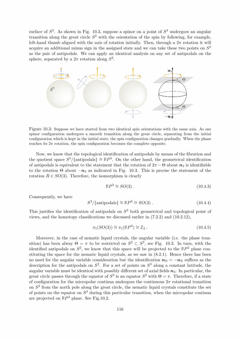
surface of S3. As shown in Fig. 10.3, suppose a spinor on a point of S3 undergoes an angulartransition along the great circle S2 with the orientation of the spin by following, for example,left-hand thumb aligned with the axis of rotation initially. Then, through a 2π rotation it willacquire an additional minus sign in the assigned state and we can take these two points on S3
as the pair of antipodals. We can apply an identical analysis on any set of antipodals on thesphere, separated by a 2π rotation along S2.
Figure 10.3: Suppose we have started from two identical spin orientations with the same axis. As onespinor configuration undergoes a smooth transition along the great circle, separating from the initialconfiguration which is kept in the initial state, the spin configuration changes gradually. When the phasereaches its 2π rotation, the spin configuration becomes the complete opposite.
Now, we know that the topological identification of antipodals by means of the fibration andthe quotient space S3/antipodals ∼= RP 3. On the other hand, the geometrical identificationof antipodals is equivalent to the statement that the rotation of 2π− Θ about n3 is identifiableto the rotation Θ about −n3 as indicated in Fig. 10.3. This is precise the statement of therotation R ∈ SO(3). Therefore, the isomorphism is clearly
RP 3 ∼= SO(3) . (10.4.3)
Consequently, we haveS3/antipodals ∼= RP 3 ∼= SO(3) . (10.4.4)
This justifies the identification of antipodals on S3 both geometrical and topological point ofviews, and the homotopy classifications we discussed earlier in (7.2.2) and (10.2.12),
π1(SO(3)) ∼= π1(RP 3) ∼= Z2 . (10.4.5)
Moreover, in the case of nematic liquid crystals, the angular variable (i.e. the phase tran-sition) has been alway Θ = π to be restricted on S2 ⊂ S3, see Fig. 10.3. In turn, with theidentified antipodals on S2, we know that this space will be projected to the RP 2 plane con-stituting the space for the nematic liquid crystals, as we saw in (8.2.1). Hence there has beenno need for the angular variable consideration but the identification nN = −nN suffices as thedescription for the antipodals on S2. For a set of points on S3 along a constant latitude, theangular variable must be identical with possibly different set of axial fields n3. In particular, thegreat circle passes through the equator of S3 is an equator S2 with Θ = π. Therefore, if a stateof configuration for the micropolar continua undergoes the continuous 2π rotational transitionon S3 from the north pole along the great circle, the nematic liquid crystals constitute the setof points on the equator on S3 during this particular transition, when the micropolar continuaare projected on RP 3 plane. See Fig.10.2.
116
Further, if we consider the element R ∈ SO(3) as the microrotation, then we can concludethe geometrical identification of antipodals are micropolar continua that live on RP 3 governedby the microrotational deformations of an angular function Θ about the position-dependentnormalised axis n3 with the nematic liquid crystals are contained in its submanifold.
We can envision the space of axial fields on the sphere, as the space filled with tiny grains ro-tating independently along with rotational angles about axes determined by parameters Θ,n3.Once we identify the antipodals on S3, these grains are projected to RP 3 constituting the mi-cropolar continua satisfying the boundary conditions we discussed in (10.2.19). Moreover, as wenoted in Section 8.4 and Section 7.2, we can regard the microrotation Rij as the order parameterin evaluating the energy functionals as we did in Section 2,
δVtotalδF
and δVtotal
δR(10.4.6)
whereV = Velastic(F,R) + Vcurvature(R) + Vinteraction(F,R) + Vcoupling(F,R) .
Since the microrotation R can be represented by an angular variable Θ and an axis vector n3,we can take the Qij , the form of isotensor Higgs field that appears in the Polyakov field (9.4.7),as the order parameter of the micropolar continua but now equipped with the integer N ,
Qij =(n3in3j − 1
3δij
)Θ , i, j = 1, 2, 3 (10.4.7)
where n3i = n3 is (9.2.25), the normalised rotational axis with the integer N in three dimensions.This leads us to the following consequences.
1. The equation of motion of (9.4.1) in (3 + 1) dimension is of the form
∂µ∂µQ = ∂2Q
∂t2− ∇2Q = −∂U
∂Q(10.4.8)
where U is the potential of the given system and ∇2 is the Laplacian operator. There existsan isomorphism of the order parameters consideration between Qij of (10.4.7) and themicrorotation Rij of (10.1.1). Then, after applying the normalisation condition n3 ·n3 = 1to remove factors of n3i in Qij , the equation of motion (10.4.8) in (1 + 1) dimensions isthe variation of Vtotal with respect to the microrotation in (10.4.6) with the kinetic term,which is just our dynamic equation of motion for the microrotational angle Θ in (1 + 1)dimensions given by (2.3.7)
∂ttΘ − ∂zzΘ + ∂U
∂Q= 0 , (10.4.9)
where U is a modified potential accordingly and z is the rescaled axis. This observa-tion reinforces the statement that our formulation in deriving the equations of motion isequivalent to the approach from the constitutive equations with order parameter given by(8.4.42) in the free energy formalism. Moreover, the form of the order parameter (10.4.7)in RP 3 for the microcontinuum is the generalised form of the order parameter (8.4.7) forthe nematic liquid crystals, both are in traceless and symmetric forms.
2. The 2π rotation will correspond to the maximum energy required in transition of thephase on S3. On the projective plane RP 3, the maximum energy required will correspondto bring a field configuration from infinity |x| = ∞ to the origin x = 0. This is theenergy difference experienced by a point of continua when it undergoes transition from
117
a total deformation-free state to its peak deformed configuration, with its maximum mi-crorotational angle before it return to its original configuration, provided the deformationoccurs in the elastic regime. Hence, when we consider the static solution of our equationof motion (2.3.17) by putting t = 0 and the phase shift δ = 0, the maximum amplitude ofthe solution is acquired at the origin, see Fig. 2.2.
3. Depending on the form of potential U , the equation of motion (10.4.9) can be either thesimple ϕ4 theory, the Klein-Gordon type, the since-Gordon type or more exotic form ofequations we saw in solving the chiral case in Chapter 3. Notably these all satisfy the finiteenergy requirement in the framework of the elasticity leading to the degenerate minimacorresponding to the distinct set of topological sectors
Θ(±∞, t) −→ Θ0 ,
for some fixed vacuum solution Θ0 which minimises the energy in the given HamiltonianH. Of course, we can set the trivial angular variable vacuum solution by Θ0 = 0, theconfiguration on the north pole of S3, to be projected to the configuration for |x| → ∞on RP 3.
4. Since SU(2) is a double cover of SO(3), we can apply the Lifting Properties of the fun-damental group to classify the various forms of defects such as monopole, vortex, anddomain walls, according to (8.1.12). For example
πn(Sn) ∼= πn(RPn) ∼= Z, n ≥ 2 , (10.4.10)
relating various possible defects in micropolar continua and spinor systems. One of suchexample is the explicit relation between Skyrmions and Nye’s tensor (10.3.5) to describethe vanishing curvature but nonzero torsion on the manifold. In words, Skyrme’s field Ba
µ
describes the gradient of the pion field through the complex doublet z on S3 and Nye’stensor describes the defect of the director field ξa of the micropolar continua on RP 3. Twodeformational descriptions on the different physical systems share the identical homotopicclassification (10.4.10), and more explicitly, the analogy can be seen in the integrationssuch as (10.3.14) and (10.3.16).
We summarise the results we obtained with corresponding homotopy classifications whichwould be useful to identify the defects in various situations. In particular, once the antipodalpoints are identified on the sphere Sn, we can write the corresponding projective space. SeeTable 10.1.
Models Sphere Projection HomotopyS1 RP 1 π1(RP 1) ∼= Z
π2(RP 1) ∼= π3(RP 1) ∼= 0Nematic liquid crystals S2 RP 2 π1(RP 2) ∼= Z2
π2(RP 2) ∼= π3(RP 2) ∼= ZMicropolar continua S3 RP 3 π1(RP 3) ∼= Z2
π2(RP 3) ∼= 0π3(RP 3) ∼= Z
Table 10.1:
We would like to conclude this Section with one additional remark on the antipodals on S3.If we are allowed to identify the antipodals, this corresponds to match two opposite rotations,
118
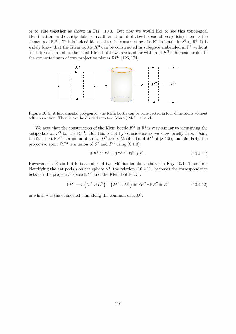
or to glue together as shown in Fig. 10.3. But now we would like to see this topologicalidentification on the antipodals from a different point of view instead of recognising them as theelements of RP 3. This is indeed identical to the constructing of a Klein bottle in S3 ⊂ R4. It iswidely know that the Klein bottle K3 can be constructed in subspace embedded in R4 withoutself-intersection unlike the usual Klein bottle we are familiar with, and K3 is homeomorphic tothe connected sum of two projective planes RP 2 [126,174].
Figure 10.4: A fundamental polygon for the Klein bottle can be constructed in four dimensions withoutself-intersection. Then it can be divided into two (chiral) Möbius bands.
We note that the construction of the Klein bottle K3 in R4 is very similar to identifying theantipodals on S3 for the RP 3. But this is not by coincidence as we show briefly here. Usingthe fact that RP 2 is a union of a disk D2 and a Möbius band M2 of (8.1.5), and similarly, theprojective space RP 3 is a union of S2 and D3 using (8.1.3)
RP 3 ∼= D3 ∪ ∂D3 ∼= D3 ∪ S2 . (10.4.11)
However, the Klein bottle is a union of two Möbius bands as shown in Fig. 10.4. Therefore,identifying the antipodals on the sphere S2, the relation (10.4.11) becomes the correspondencebetween the projective space RP 3 and the Klein bottle K3,
RP 3 −→(M2 ∪D2
)∪(M2 ∪D2
)∼= RP 2 ∗ RP 2 ∼= K3 (10.4.12)
in which ∗ is the connected sum along the common disk D2.
119

120
Chapter 11
Conclusions and outlooks
Soliton solutions are obtained in Part I from the variational principle after collecting the mostgeneral energy functionals with the set of appropriate coupling moduli. These soliton solutionsare descriptions for the coupled system of microscopic and macroscopic deformations both underthe achiral and chiral energy considerations. As the chiral solution, we specified the requirementsfor chiral energy functionals in the higher dimensions by investigating the inversion propertiesof the individual characteristic deformational measures, such as rotations, translations anddeformation gradient tensors. We found that the dislocation density tensor K = RT CurlRis one of the suitable measures for this purpose among other possible combinations of chiral-inducible energy functionals.
In Part II, we found that the dislocation density tensor played the central role along with thecontortion tensor in the manifold where both curvature and torsion are permissible. Within thescope of vanishing curvature, we derived and reinterpreted the compatibility conditions bothfor vanishing torsion and non-vanishing torsion. The general expression for the Einstein tensorin the Riemann-Cartan manifold gave us a unique opportunity to understand the universalgeometrical process to derive various forms of the compatibility conditions. These are widelyapplicable in micromorphic continua and the Skyrme model we studied in Part III within theframework of the Einstein-Cartan theory.
We also observed there are distinct classifications in the field configurations under the con-dition of the vanishing curvature by the simple homotopic consideration to obtain two distinctclasses such as 0 and 1. The former defines the diffeomorphic deformational class and thelatter is for the non-trivial torsion space which cannot be described by the metric tensor.
In Part III, we considered the criteria for the systems with soliton solutions under thefinite energy requirement in connection with the elastic asymptotic conditions. This led usto understand the topological and geometrical origins of the conserved current in the generaldimensions in such a way that the integer N , originated from the vortex field in two dimensions,can be embedded to the field configuration in the higher dimensions. This further yields thetotal charge, in the form of the integration of the current, is again the topologically invariantas integers N in agreement with the finite energy requirement. We found that these conservedtopological invariants correspond to the homotopic classification, and conserved charge in thevarious dimensions and physical models such as the ϕ4 theory, the Klein-Gordon system, andthe sine-Gordon system. These are the topologically stable defects within the given sectordetermined by the associated charge Q = N .
In Part I, we made use of a number of ansatz simplifying the situation to obtain the solutionsboth analytically and numerically. The ansatz included the same velocities in the microscopicand macroscopic deformational propagations and a fixed microrotational axis. Noting that thegeneral micropolar continua can be occupied by the field of position-dependent axial vectors for
121
the microrotations in inhomogeneous settings, we derived the conserved currents associated tothe topological invariants which can be written in terms of normalised axial field configurationsin various dimensions. In particular, to serve the role in the representations of the rotationalmatrix Rij equipped with the non-trivial vortex field embedded in it.
After establishing a firm relation between the nematic liquid crystals on S2 and the projec-tive plane RP 2, by identifying the antipodals in its topological and geometrical implications,we briefly considered the role of order parameter in homotopic consideration to re-derive thetopological invariants N in the theory of defects such as monopole, vortex and domain wall bytracing the possible defect that can occur in the given order parameter space.
The free energy formulation in terms of order parameter in the classical nematic liquidcrystals and in the theory of the micropolar continuum led us to generalise the order parameterof the Higgs isovector in the form of the order parameter that we can use in the micropolartheory. This is consistently applicable to the previously obtained soliton solutions. Theseare followed by the investigation on the viability of the hedgehog field configuration in threedimensions both for our micropolar model and the Skyrme model supported by the relationbetween the defect measures of pion fields and Nye’s tensor, of which can be written in theidentical form of the compatibility condition we obtained in Part II.
The geometrical considerations on S2 confirms that the nematic liquid crystals can be re-garded to be defined on the RP 2 plane with the help of the rather simple assignment of thedirectors to its molecular nature, by identifying the antipodals on the sphere. As the extensionof the identification between S2 and RP 2, we chose the model on S3 as the Skyrmions basedon the fact that the spin-isospin symmetry of two independently acting SO(3) constitutes thetransformation of SU(2). And this consequently yields the realisation that the projective planeRP 3 is for the micropolar continua when we identify the antipodals on S3. This comes nat-urally through the Hopf fibration between SU(2) and SO(3). Along with the Hopf fibration,this correspondence links the pion fields as represented by the complex doublet on C2 and n3as the axial fields for the microrotations in the projective space. This again enters into themicrorotational matrix Rij as the components of n4 field, with the topological invariant N andan additional angular variable, to identify that the antipodals on S3 is the microrotations forthe micropolar continua.
We obtained the soliton solutions in Part I and Part II without the specifications of ther-modynamic effects, dissipative factors, chemical potentials, electromagnetic interferences or thegravitational attraction to the media. Hence in reality, considering all possible such effects, thesoliton solution may lose its characteristic feature of propagating without changing its waveform, not to mention the potential interference from each other when one considers the multi-soliton systems. But if we consider the deformational propagation in a specific physical systemsuch as the continuum consideration in vacuum or a perfect fluid in a low temperature, we mighthope to obtain the relevant results we obtained here. For that purpose, we believe the tech-niques developed in this work to be applicable to certain phases of liquid superfluid helium asgood candidates which also possess the spin-orbit symmetry that can be separately representedby SO(3) both in isotropic and anisotropic settings.
122

Appendix A
Variations of energy functionals
We would like to vary each energy functional using some of identities listed in Notation andAppendix. First, for Velastic, we can expand the expression using the definition of ∥X∥2 =⟨X,X⟩ = tr(XXT ) and symM = 1/2(M +MT ) as
Velastic(F,R) = µ∥∥∥sym(RT
F − 1)∥∥∥2
+ λ
2[tr(sym(RT
F − 1))]2
=(
3µ+ 92λ)
+ 12µtr
(R
TFR
TF)
+ 12µtr(FF T ) − (2µ+ 3λ) tr(RT
F ) + λ
2[tr(RT
F )]2
.
(A.0.1)
Variation of this is
δVelastic(F,R) =[µ(RF TR+ F ) − (2µ+ 3λ)R+ λtr(RT
F )R]
: δF
+[µFR
TF − (2µ+ 3λ)F + λtr(RT
F )F]
: δR.(A.0.2)
If we want to study the dynamical problem, we must take the kinetic term into account in theelastic energy functional
Velastic,kinetic = 12ρ∥φ∥2 , (A.0.3)
where ρ is the constant density and φ is the deformation vector. If we vary this term we willobtain
δVelastic,kinetic = −ρφ δφ . (A.0.4)
But, since ∇φ = 1 + ∇u implies δφ = δu and φ = u, the variation of the elastic kinetic termcan be rewritten as δVelastic,kinetic = −ρu δu, and the variation of dynamical expression for theelastic energy functional becomes
δVelastic(F,R) =[µ(RF TR+ F ) − (2µ+ 3λ)R+ λtr(RT
F )R]
: δF
+[µFR
TF − (2µ+ 3λ)F + λtr(RT
F )F]
: δR+ ρu δu .(A.0.5)
Similarly, for the curvature functional, we can expand it as
Vcurvature(R) = (κ1 − κ2)2 tr
[R
T (CurlR)RT (CurlR)]
+ (κ1 + κ2)2 tr
[(CurlR)T (CurlR)
]−(κ1
3 − κ3)(
tr[R
T (CurlR)])2
.
(A.0.6)
123
This is a functional dependent only on R, but the actual variation will involve rather complicatedquantities such as δCurlR multiplied by a tensor. To overcome this problem, we introduce thefollowing identity. Let A(R) and B(R) be two matrix valued functions depending on the rotationR. Then, by a direct calculation, one can show that an identity for any rank-two tensors A andB,
tr(A)B : δ(CurlR) = −[B(grad tr(A)
)⋆] : δR+ tr(A)CurlB : δR (A.0.7)
where (grad tr(A)
)⋆ik
= ϵijk∂jtr(A) . (A.0.8)
The identity (A.0.7) can be shown if one uses the convention
CurlB = ϵjrsBis,rei ⊗ ej = −B,i × ei .
In particular, if we put A = 1 then (A.0.7) reduces to
B : δ(CurlR) = CurlB : δR . (A.0.9)
And this will play an important role in simplifying the calculation of variation of the energyfunctionals significantly. For example, the first variational term in (A.0.6) would be
δ(tr[R
T (CurlR)RT (CurlR)])
= 2[R(CurlR)TR
]: δ(CurlR) + 2(CurlR)RT (CurlR) : δR
= 2(Curl
[R(CurlR)TR
]+ (CurlR)RT (CurlR)
): δR .
(A.0.10)
In this way, we find the variation of the curvature term
δVcurvature(R) =[(κ1−κ2)
((CurlR)RT (Curl (R))+Curl
[R(CurlR)TR
])+(κ1+κ2)Curl
[CurlR
]−(κ13 − κ3
)(4tr(RT CurlR)Curl (R) − 2R
(grad
(tr[RT CurlR]
))⋆]: δR . (A.0.11)
Again, for the dynamical case, we need to include the kinetic term defined as
Vcurvature,kinetic = ρrot∥R∥2 = ρrottr(R RT ) (A.0.12)
with variational form given by δVcurvature,kinetic = −2ρrotR : δR.Therefore, the variation of dynamical expression for the curvature energy functional can bewritten as
δVcurvature(R) =[(κ1−κ2)
((CurlR)RT (Curl (R))+Curl
[R(CurlR)TR
])+(κ1+κ2)Curl
[CurlR
]−(κ13 − κ3
)(4tr(RT CurlR)Curl (R) − 2R
(grad
(tr[RT CurlR]
))⋆+ 2ρrotR
]: δR . (A.0.13)
For the interaction energy functional, we expand terms dev sym(RT CurlR) and dev sym(RTF−
1) to write
Vinteraction =(χ1 − χ3
3
)tr(RT CurlR)tr(RT
F )
+ χ32(tr[(CurlR)TF
]+ tr
[R
T (CurlR)RTF])
.
(A.0.14)
124
The variation of this involves the quantity δCurlR as in the case of Vcurvature, so we use theidentity (A.0.9) to obtain
δVinteraction(F,R) =(χ1 − χ3
3)(
2tr(RTF )CurlR+ tr(RT CurlR)F −R
[grad
(tr[RT
F ])]⋆)
+ χ32(CurlF + (CurlR)RT
F + FRT (CurlR) + Curl (RF TR)
): δR
+χ1tr(RT CurlR)R+ χ3
2(CurlR+R(CurlR)TR
)− χ3
3 tr(RT CurlR)R
: δF . (A.0.15)
We write the coupling energy functional as
Vcoupling(F,R) = µc
∥∥∥RT polar(F ) − 1∥∥∥2
= 2µc(3 − tr[RT polar(F )]) . (A.0.16)
We note that this depends on R and R = polar(F ), hence depends on R and F . Therefore, thevariation of coupling energy functional is of the form
δVcoupling(F,R) = −2µcR : δR− 2µc
[∂
∂F
(tr[RT
R])]
: δF . (A.0.17)
The term in the brackets in the second term can be written as∂
∂F
(tr[RT
R])
=( dR
dFml
): ∂
∂R
[tr(RT
R)]
=( dR
dFml
): R = 1
det(Y )[RY (RTR−R
TR)Y
](A.0.18)
where Y = tr(U)1−U . In the first step, we used the chain rule, and in the second and last stepswe used the identities given in (A.0.21). Then the variation of the coupling energy becomes
δVcoupling(F,R) = −2µcR : δR− 2µc
det(Y )[RY (RTR−R
TR)Y
]: δF . (A.0.19)
Lastly, we vary the chiral energy functional Vχ = χtr(K3) as follows
δVχ = 3χ(K2)T : δK = 3χ[(K2)T
ijδ(RT CurlR)ij
]= 3χ
[(K2)T
ij
(δRmi(CurlR)mj +Rmi(δCurlR)mj
)]= 3χ
[(CurlR)mj(K2)T
ijδRmi +Rmi(K2)T
ij(δCurlR)mj
]= 3χ
[(CurlR)(K2) : δR+R(K2)T : δCurlR
]= 3χ
[(CurlR)(K2) : δR+ Curl [R(K2)T ] : δR
]= 3χ
[(CurlR)(K2) + Curl [R(K2)T ]
]: δR .
(A.0.20)We list some useful matrix identities below.
∂
∂Xtr(F (X)) = [f(X)]T ,
∂
∂Xtr(X) = I ,
∂
∂Xtr(XA) = AT ,
∂
∂Xtr(AXB) = ATBT ,
d
dX(tr(XXT )) = 2X ,
d
dX(tr(XA)) = AT ,
(A.0.21)
andd
dX(tr(AXBX)) = ATXTBT +BTXTAT ,
dg(R(F ))Fml
= tr[dR
dFml
(dg(R)dR
)T]
= dR
dFml:(dg(R)dR
),
(A.0.22)
where f stands for the scalar derivative of F .
125

126
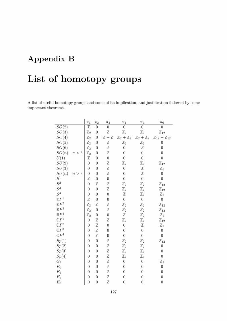
Appendix B
List of homotopy groups
A list of useful homotopy groups and some of its implication, and justification followed by someimportant theorems.
π1 π2 π3 π4 π5 π6SO(2) Z 0 0 0 0 0SO(3) Z2 0 Z Z2 Z2 Z12SO(4) Z2 0 Z + Z Z2 + Z2 Z2 + Z2 Z12 + Z12SO(5) Z2 0 Z Z2 Z2 0SO(6) Z2 0 Z 0 Z 0SO(n) n > 6 Z2 0 Z 0 0 0U(1) Z 0 0 0 0 0SU(2) 0 0 Z Z2 Z2 Z12SU(3) 0 0 Z 0 Z Z6SU(n) n > 3 0 0 Z 0 Z 0S1 Z 0 0 0 0 0S2 0 Z Z Z2 Z2 Z12S3 0 0 Z Z2 Z2 Z12S4 0 0 0 Z Z2 Z2RP 1 Z 0 0 0 0 0RP 2 Z2 Z Z Z2 Z2 Z12RP 3 Z2 0 Z Z2 Z2 Z12RP 4 Z2 0 0 Z Z2 Z2CP 1 0 Z Z Z2 Z2 Z12CP 2 0 Z 0 0 Z Z2CP 3 0 Z 0 0 0 0CP 4 0 Z 0 0 0 0Sp(1) 0 0 Z Z2 Z2 Z12Sp(2) 0 0 Z Z2 Z2 0Sp(3) 0 0 Z Z2 Z2 0Sp(4) 0 0 Z Z2 Z2 0G2 0 0 Z 0 0 Z3F4 0 0 Z 0 0 0E6 0 0 Z 0 0 0E7 0 0 Z 0 0 0E8 0 0 Z 0 0 0
127
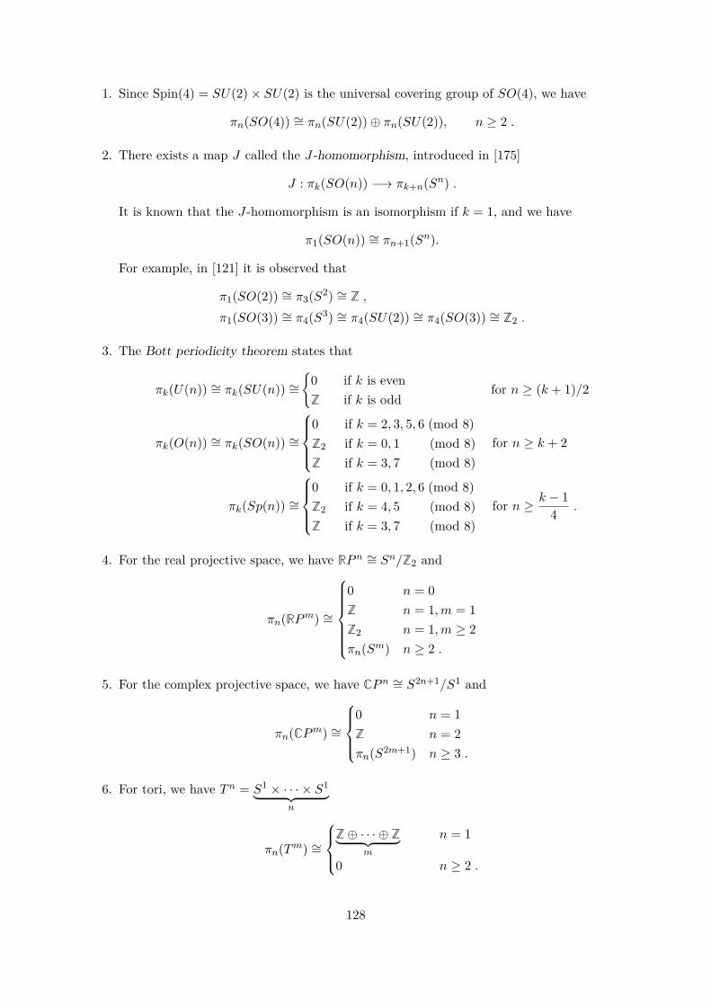
1. Since Spin(4) = SU(2) × SU(2) is the universal covering group of SO(4), we have
πn(SO(4)) ∼= πn(SU(2)) ⊕ πn(SU(2)), n ≥ 2 .
2. There exists a map J called the J-homomorphism, introduced in [175]
J : πk(SO(n)) −→ πk+n(Sn) .
It is known that the J-homomorphism is an isomorphism if k = 1, and we have
π1(SO(n)) ∼= πn+1(Sn).
For example, in [121] it is observed that
π1(SO(2)) ∼= π3(S2) ∼= Z ,
π1(SO(3)) ∼= π4(S3) ∼= π4(SU(2)) ∼= π4(SO(3)) ∼= Z2 .
3. The Bott periodicity theorem states that
πk(U(n)) ∼= πk(SU(n)) ∼=
0 if k is evenZ if k is odd
for n ≥ (k + 1)/2
πk(O(n)) ∼= πk(SO(n)) ∼=
0 if k = 2, 3, 5, 6 (mod 8)Z2 if k = 0, 1 (mod 8)Z if k = 3, 7 (mod 8)
for n ≥ k + 2
πk(Sp(n)) ∼=
0 if k = 0, 1, 2, 6 (mod 8)Z2 if k = 4, 5 (mod 8)Z if k = 3, 7 (mod 8)
for n ≥ k − 14 .
4. For the real projective space, we have RPn ∼= Sn/Z2 and
πn(RPm) ∼=
0 n = 0Z n = 1,m = 1Z2 n = 1,m ≥ 2πn(Sm) n ≥ 2 .
5. For the complex projective space, we have CPn ∼= S2n+1/S1 and
πn(CPm) ∼=
0 n = 1Z n = 2πn(S2m+1) n ≥ 3 .
6. For tori, we have Tn = S1 × · · · × S1︸ ︷︷ ︸n
πn(Tm) ∼=
Z ⊕ · · · ⊕ Z︸ ︷︷ ︸
m
n = 1
0 n ≥ 2 .
128
Bibliography
[1] C. G. Böhmer, Y. Lee, and P. Neff. Soliton solutions in geometrically nonlinear Cosseratmicropolar elasticity with large deformations. Wave Motion, 84:110–124, 2019.
[2] C. G. Böhmer, Y. Lee, and P. Neff. Chirality in the plane. J. Mech. Phys. Solids,134:103753, 2020.
[3] E. Cosserat and F. Cosserat. Théorie des corps déformables. Librairie Scientifique A,Hermann et Fils, 1909.
[4] E. Whittaker. A History of the Theories of Aether and Electricity. Thomas Nelson andSons, 1951.
[5] J. L. Ericksen and C. Truesdell. Exact theory of stress and strain in rods and shells. Arch.Rational Mech. Anal., 1:295–323, 1957.
[6] R. A. Toupin. Elastic materials with couple-stresses. Arch. Rational Mech. Anal., 11:385–414, 1962.
[7] J. L. Ericksen. Hydrostatic theory of liquid crystals. Arch. Rational Mech. Anal., 9:379–394, 1962.
[8] A. E. Green. Multipolar continuum mechanics. Arch. Rational Mech. Anal, 17:113–147,1964.
[9] A. C. Eringen and E. S. Suhubi. Nonlinear theory of simple microelastic solids I. Int. J.Eng. Sci, 2:189–204, 1964.
[10] R. D. Mindlin. Micro-structure in linear elasticity. Arch. Rational Mech. Anal., 16(1):51–78, 1964.
[11] R. A. Toupin. Theories of elasticity with couple-stress. Arch. Rational Mech. Anal.,17:85–112, 1964.
[12] H. Schaefer. Das Cosserat Kontinuum. Z. Angew. Math. Mech., 47:485–498, 1967.
[13] J. L. Ericksen. Twisting of liquid crystals. J. Fluid Mech., 27:59–64, 1967.
[14] A. C. Eringen and E. S. Suhubi. Nonlinear theory of simple microelastic solids II. Int. J.Eng. Sci, 2:389–404, 1964.
[15] A. C. Eringen. Microcontinuum field theories: I. Foundations and solids. Springer, 1999.
[16] P. Neff. Existence of minimizers for a finite-strain micromorphic elastic solid. Proc. Roy.Soc. Edinb. A, 136:997–1012, 2006.
129
[17] P. Neff and I. Münch. Curl bounds Grad on SO(3). ESAIM Control Optim. Calc. Var.,14(1):148–159, 2008.
[18] P. Neff. Existence of minimizers in nonlinear elastostatics of micromorphic solids. InD. Iesan, editor, Encyclopedia of Thermal Stresses. Springer, Heidelberg, 2013.
[19] P. Neff, I. D. Ghiba, M. Lazar, and A. Madeo. The relaxed linear micromorphic continuum:well-posedness of the static problem and relations to the gauge theory of dislocations. Q.J. Mech. Appl. Math., 68(1):53–84, 2015.
[20] M. Bîrsan and P. Neff. On the dislocation density tensor in the Cosserat theory of elasticshells. In Advanced Methods of Continuum Mechanics for Materials and Structures, pages391–413. Springer, 2016.
[21] C. G. Böhmer, R. J. Downes, and D. Vassiliev. Rotational elasticity. Q. J. MechanicsAppl. Math., 64(4):415–439, 2011.
[22] C. G. Böhmer and Y. N. Obukhov. A gauge-theoretic approach to elasticity with micro-rotations. Proc. R. Soc. A, 468(1391-1407), 2012.
[23] C. G. Böhmer and N. Tamanini. Rotational elasticity and couplings to linear elasticity.Math. Mech. Solids, 20(8):959–974, 2013.
[24] S. Bahamonde, C. G. Böhmer, and P. Neff. Geometrically nonlinear Cosserat elasticityin the plane: applications to chirality. J. Mech. Mater. Struct., 12(5):689–710, 2017.
[25] G. A. Maugin and A. Miled. Solitary waves in elastic ferromagnets. Phys. Rev. B,33(7):4830–4842, 1986.
[26] G. A. Maugin and A. Miled. Solitary waves in micropolar elastic crystals. Int. J. Eng.Sci., 24(9):1477–1499, 1986.
[27] A. Fischle, P. Neff, and D. Raabe. The relaxed-polar mechanism of locally optimalCosserat rotations for an idealized nanoindentation and comparison with 3D-EBSD ex-periments. Z. Angew. Math. Phys., 68(4):90, 2017.
[28] D. Iesan and L. Nappa. Extremum principles and existence results in micromorphicelasticity. Int. J. Eng. Sci., 39(18):2051–2070, 2001.
[29] S. Forest. Micromorphic approach for gradient elasticity, viscoplasticity, and damage. J.Eng. Mech., 135(3):117–131, 2009.
[30] P. Neff, I. D. Ghiba, A. Madeo, L. Placidi, and G. Rosi. A unifying perspective: therelaxed linear micromorphic continuum. Cont. Mech. Thermodyn., 26:639–681, 2014.
[31] P. Neff, M. Bîrsan, and F. Osterbrink. Existence theorem for geometrically nonlinearCosserat micropolar model under uniform convexity requirements. J. Elast., 121(1):119–141, 2015.
[32] L. D. Landau and E. M. Lifshitz. Theory of Elasticity: Vol. 7 of Course of TheoreticalPhysics. Elsevier, New York, 1986.
[33] P. B. Burt. Exact, multiple soliton solutions of the double sine Gordon equation. Proc.R. Soc. Lond. A., 359:479–495, 1978.
130

[34] J. F. Nye. Some geometrical relations in dislocated crystals. Acta metallurgica, 1(2):153–162, 1953.
[35] G. Capriz. Continua with microstructure, volume 35. Springer-Verlag, New York, 1989.
[36] R. D. Mindlin and H. F. Tiersten. Effects of couple-stresses in linear elasticity. Arch.Ration. Mech. Anal., 11:415–448, 1962.
[37] I. Münch, W. Wagner, and P. Neff. Constitutive modeling and FEM for a nonlinearCosserat continuum. In PAMM: Proc. Appl. Math. Mech, volume 6, pages 499–500, 2006.
[38] P. Neff. The Cosserat couple modulus for continuous solids is zero viz the linearizedCauchy-stress tensor is symmetric. ZAMM-Z. Angew. Math. Mech., 86(11):892–912, 2006.
[39] C. G. Böhmer, P. Neff, and B. Seymenoglu. Soliton-like solutions based on geometricallynonlinear Cosserat micropolar elasticity. Wave Motion, 60:158–165, 2016.
[40] R. Rajaraman. Solitons and instantons. North-Holland, Netherlands, 1982.
[41] S. W. Smith. Chiral toxicology: it’s the same thing. . . only different. Toxicol. Sci.,110(1):4–30, 2009.
[42] R. S. Lakes and R. L. Benedict. Noncentrosymmetry in micropolar elasticity. Int. J. Eng.Sci., 20(10):1161–1167, 1982.
[43] A. Spadoni and M. Ruzzene. Elasto-static micropolar behavior of a chiral auxetic lattice.J. Mech. Phys. Solids, 60(1):156–171, 2012.
[44] X. N. Liu, G. L. Huang, and G. K. Hu. Chiral effect in plane isotropic micropolar elasticityand its application to chiral lattices. J. Mech. Phys. Solids, 60(11):1907–1921, 2012.
[45] R. S. Lakes. Elastic and viscoelastic behavior of chiral materials. Int. J. Mech. Sci.,43(7):1579–1589, 2001.
[46] S. A. Papanicolopulos. Chirality in isotropic linear gradient elasticity. Int. J. SolidsStruct., 48(5):745–752, 2011.
[47] K. J. Cheverton and M. F. Beatty. Extension, torsion and expansion of an incompressible,hemitropic Cosserat circular cylinder. J. Elast., 11(2):207–227, 1981.
[48] X. N. Liu, G. L. Huang, and G. K. Hu. Analytical formulation of a discrete chiral elasticmetamaterial model. In Health Monitoring of Structural and Biological Systems 2012,volume 8348, pages 834–823. International Society for Optics and Photonics, 2012.
[49] X. N. Liu and G. K. Hu. Elastic metamaterials making use of chirality: a review. Strojniškivestnik-J. Mech. Eng., 62(7-8):403–418, 2016.
[50] Y. Chen, X. Liu, and G. Hu. Micropolar modeling of planar orthotropic rectangular chirallattices. Comptes Rendus Mécanique, 342(5):273–283, 2014.
[51] V. A. Fedotov, P. L. Mladyonov, S. L. Prosvirnin, A. V. Rogacheva, Y. Chen, and N. I.Zheludev. Asymmetric propagation of electromagnetic waves through a planar chiralstructure. Phys. Rev. Lett., 97(16):167401, 2006.
[52] A. Papakostas, A. Potts, D. M. Bagnall, S. L. Prosvirnin, H. J. Coles, and N. I. Zheludev.Optical manifestations of planar chirality. Phys. Rev. Lett., 90(10):107404, 2003.
131
[53] W. Zhang, A. Potts, and D. M. Bagnall. Giant optical activity in dielectric planar meta-materials with two-dimensional chirality. J. Opt. A, 8(10):878, 2006.
[54] X. Ma, C. Huang, M. Pu, Y. Wang, Z. Zhao, C. Wang, and X. Luo. Dual-band asymmetrychiral metamaterial based on planar spiral structure. Appl. Phys. Lett., 101(16):161901,2012.
[55] Z. Li, M. Gokkavas, and E. Ozbay. Manipulation of asymmetric transmission in planarchiral nanostructures by anisotropic loss. Adv. Opt. Mater., 1(7):482–488, 2013.
[56] O. Arteaga, J. Sancho-Parramon, S. Nichols, B. M. Maoz, A. Canillas, S. Bosch,G. Markovich, and B. Kahr. Relation between 2d/3d chirality and the appearance ofchiroptical effects in real nanostructures. Opt. Express, 24(3):2242–2252, 2016.
[57] D. Prall and R. S. Lakes. Properties of a chiral honeycomb with a Poisson’s ratio of 1.Int. J. Mech. Sci., 39(3):305–314, 1997.
[58] Y. Chen, X. N. Liu, G. Hu, and Q. Sunand Q. Zheng. Micropolar continuum modellingof bi-dimensional tetrachiral lattices. Proc. R. Soc. Lond. A, 470(2165):20130734, 2014.
[59] W. Zhang, R. Neville, D. Zhang, F. Scarpa, L. Wang, and R. Lakes. The two-dimensionalelasticity of a chiral hinge lattice metamaterial. Int. J. Solids Struct., 141:254–263, 2018.
[60] R. Raval. Chiral expression from molecular assemblies at metal surfaces: insights fromsurface science techniques. Chem. Soc. Rev., 38(3):707–721, 2009.
[61] F. Chiadini, V. Fiumara, T. G. Mackay, A. Scaglione, and A. Lakhtakia. Left/rightasymmetry in Dyakonov-Tamm-wave propagation guided by a topological insulator anda structurally chiral material. J. Opt., 18(11):115101, 2016.
[62] D. Ieşan. Thermoelastic deformation of reinforced chiral cylinders. Acta Mechanica, 228,07 2017.
[63] W. Wu, D. Qi, H. Liao, G. Qian, L. Geng, Y. Niu, and J. Liang. Deformation mechanismof innovative 3d chiral metamaterials. Sci. Rep., 8(1):12575, 2018.
[64] H. Joumaa and M. Ostoja-Starzewski. Stress and couple-stress invariance in non-centrosymmetric micropolar planar elasticity. Proc. R. Soc. Lond. A, 467(2134):2896–2911, 2011.
[65] I. Münch and P. Neff. Rotational invariance conditions in elasticity, gradient elasticityand its connection to isotropy. Math. Mech. Solids, 23(1):3–42, 2018.
[66] K. Kondo. On the analytical and physical foundations of the theory of dislocations andyielding by the differential geometry of continua. Int. J. Engng. Sci., 2(3):219–251, 1964.
[67] R. deWit. Relation between Dislocations and Disclinations. J. Appl. Phys., 42(9):3304–3308, 1971.
[68] M. Kléman. Relationship between Burgers circuit, Volterra process and homotopy groups.Journal de Physique Lettres, 38(10):199–202, 1977.
[69] M. Kléman. Defects in liquid crystals. Rep. Prog. Phys., 52(5):555–654, May 1989.
[70] C. N. Yang and R. L. Mills. Conservation of isotopic spin and isotopic gauge invariance.Phys. Rev., 96(1):191, 1954.
132
[71] R. Utiyama. Invariant theoretical interpretation of interaction. Phys. Rev., 101(5):1597,1956.
[72] T. W. B. Kibble. Lorentz invariance and the gravitational field. J. Math. Phys., 2(2):212–221, 1961.
[73] S. Deser and B. Zumino. Consistent supergravity. Phys. Lett. B, 62(3):335–337, 1976.
[74] F. W. Hehl, P. Von Der Heyde, G. D. Kerlick, and J. M. Nester. General Relativity withSpin and Torsion: Foundations and Prospects. Rev. Mod. Phys., 48:393–416, 1976.
[75] S. Hojman, M. Rosenbaum, M. P. Ryan, and L. C. Shepley. Gauge invariance, minimalcoupling, and torsion. Phys. Rev. D, 17(12):3141, 1978.
[76] A. H. Cottrell and B. A. Bilby. Dislocation theory of yielding and strain ageing of iron.Proc. Phys. Soc. A, 62(1):49, 1949.
[77] E. Kröner. Allgemeine kontinuumstheorie der versetzungen und eigenspannungen. Arch.Rational Mech. Anal., 4(1):273, 1959.
[78] W. Noll. A mathematical theory of the mechanical behavior of continuous media. Arch.Rational Mech. Anal., 2(1):197–226, 1958.
[79] B. A. Bilby. Geometry and continuum mechanics. In Mechanics of Generalized Continua,pages 180–199. Springer, 1968.
[80] H. Kleinert. Gravity as a Theory of Defects in a Crystal with Only Second GradientElasticity. Ann. Phys., 499(2):117–119, 1987.
[81] M. O. Katanaev and I. V. Volovich. Theory of defects in solids and three-dimensionalgravity. Ann. Phys., 216(1):1–28, 1992.
[82] F. W. Hehl and Y. N. Obukhov. Élie Cartan’s torsion in geometry and in field theory, anessay. Annales Fond. Broglie, 32:157–194, 2007.
[83] A. Yavari and A. Goriely. Riemann-Cartan geometry of nonlinear dislocation mechanics.Arch. Rational Mech. Anal., 205(1):59–118, 2012.
[84] A. Yavari and A. Goriely. Riemann-Cartan geometry of nonlinear disclination mechanics.Math. Mech. Solids, 18(1):91–102, 2013.
[85] H. I. Arcos and J. G. Pereira. Torsion gravity: a reappraisal. Int. J. Mod. Phys. D,13(10):2193–2240, 2004.
[86] C. G. Böhmer and R. J. Downes. From continuum mechanics to general relativity. Int.J. Mod. Phys. D, 23(12):1442015, 2014.
[87] R. Aldrovandi and J. G. Pereira. Teleparallel Gravity: An Introduction, volume 173.Springer, Dordrecht Heidelberg New York London, 2013.
[88] M. Lazar and F. W. Hehl. Cartan’s spiral staircase in physics and, in particular, in thegauge theory of dislocations. Found. Phys., 40(9-10):1298–1325, 2010.
[89] H. Kleinert. New gauge symmetry in gravity and the evanescent role of torsion. InProceedings Of The Conference In Honour Of Murray Gell-Mann’s 80th Birthday, pages174–185. World Scientific, 2011.
133
[90] M. Blagojević and F. W. Hehl. Gauge Theories of Gravitation: A Reader with Commen-taries. Imperial Collge Press, 2013.
[91] H. Kleinert and J. Zaanen. Nematic world crystal model of gravity explaining absence oftorsion in spacetime. Phys. Lett. A, 324(5-6):361–365, 2004.
[92] A. J. Beekman, J. Nissinen, K. Wu, K. Liu, R. Slager, Z. Nussinov, V. Cvetkovic, andJ. Zaanen. Dual gauge field theory of quantum liquid crystals in two dimensions. Phys.Rep., 683:1–110, 2017.
[93] J. Nissinen. Emergent Spacetime and Gravitational Nieh-Yan Anomaly in Chiral p + ipWeyl Superfluids and Superconductors. Phys. Rev. Lett., 124(11):117002, 2020.
[94] I. Peshkov, E. Romenski, and M. Dumbser. Continuum mechanics with torsion. Contin-uum Mech. Thermodyn., 31(5):1517–1541, 2019.
[95] J. Nissinen and G. E. Volovik. Tetrads in solids: from elasticity theory to topologicalquantum Hall systems and Weyl fermions. J. Exp. Theor. Phys., 127(5):948–957, 2018.
[96] J. Nissinen and G. E. Volovik. Elasticity tetrads, mixed axial-gravitational anomalies,and (3+1)-d quantum Hall effect. Phys. Rev. Research, 1(023007), September 2019.
[97] A. D. Sakharov. Vacuum quantum fluctuations in curved space and the theory of gravi-tation. Soviet Physics Uspekhi, 34(5):394, 1991.
[98] B. A. Bilby, R. Bullough, and E. Smith. Continuous distributions of dislocations: anew application of the methods of non-Riemannian geometry. Proc. R. Soc. Lond. A,231(1185):263–273, 1955.
[99] K. Kondo. Non-Riemannian and Finslerian approaches to the theory of yielding. Int. J.Engng. Sci., 1(1):71–88, 1963.
[100] S. K. Godunov and E. I. Romenskii. Nonstationary equations of nonlinear elasticity theoryin Eulerian coordinates. J. Appl. Mech. Tech. Phys., 13(6):868–884, 1972.
[101] E. Kröner. Continuum theory of defects, in Physics of defects (Les Houches, Session 35),ed. R. Balian et al. North-Holland, Amsterdam, 1980.
[102] H. Kleinert. Gauge Fields in Condensed Matter Vol. 2: Stresses and Defects (DifferentialGeometry, Crystal Melting). World Scientific, Singapore, 1989.
[103] S. K. Godunov and E. Romenskii. Elements of continuum mechanics and conservationlaws. Kluwer Academic/Plenum Publishers, New York, 2003.
[104] C. G. Böhmer and Y. Lee. Compatibility conditions of continua using Riemann-Cartangeometry. Math. Mech. Solids, 2020.
[105] C. Vallée. Compatibility equations for large deformations. Int. J. Eng. Sci, 30(12):1753–1757, 1992.
[106] P. G. Ciarlet, L. Gratie, O. Iosifescu, C. Mardare, and C. Vallée. Another approach to thefundamental theorem of Riemannian geometry in R3, by way of rotation fields. J. Math.Pures. Appl., 87(3):237–252, 2007.
[107] H. Poincaré. Sur les propriétés des fonctions définies par les équations aux différencespartielles. Number 432. Gauthier-Villars, 1879.
134
[108] D. G. B. Edelen. A new look at the compatability problem of elasticity theory. Int. J.Engng. Sci., 28(1):23–27, 1990.
[109] A. Trautman. Fibre bundles associated with space-time. Rep. Math. Phys., 1(1):29–62,1970.
[110] J. Lankeit, P. Neff, and F. Osterbrink. Integrability conditions between the first andsecond Cosserat deformation tensor in geometrically nonlinear micropolar models andexistence of minimizers. Z. Angew. Math. Mech., 68(1):11, 2016.
[111] H. Kleinert. Towards a unified field theory of defects and stresses. Lettere al NuovoCimento, 35(2):41–45, 1982.
[112] J. A. Schouten. Ricci-Calculus. Springer, Berlin, Heidelberg, 1954.
[113] R. M. Wald. General relativity. University of Chicago press, Chicago, 1984.
[114] C. W. Misner, K. S. Thorne, and J. A. Wheeler. Gravitation. W. H. Freeman andCompany, New York, 1999.
[115] R. deWit. Theory of disclinations: II. Continuous and discrete disclinations in anisotropicelasticity. J. Res. Natl. Bur. Stand. A Phys. Chem., 77(1):49, 1973.
[116] M. Nakahara. Geometry, topology and physics. IOP Publishing, Bristol and Philadelphia,2003.
[117] R. deWit. Theory of disclinations: II. Continuous and discrete disclinations in isotropicelasticity. J. Res. Nat. Stand. Sec. A, 77A(1):49, Jan 1973.
[118] P. G. Ciarlet. An introduction to differential geometry with applications to elasticity. J.Elast., 78(1-3):1–125, 2005.
[119] D. Finkelstein. Kinks. J. Math. Phys., 7(7):1218–1225, 1966.
[120] R. Shankar. Applications of topology to the study of ordered systems. Journal dePhysique, 38(11):1405–1412, 1977.
[121] M. Nakahara. Toy-Skyrmions in Superfluid 3He-A. Prog. Theor. Phys., 77(5):1011–1013,1987.
[122] M. V. Kurik and O. D. Lavrentovich. Defects in liquid crystals: homotopy theory andexperimental studies. Physics-Uspekhi, 31(3):196–224, 1988.
[123] M. Kleman and O. D. Lavrentovich. Topological point defects in nematic liquid crystals.Philos. Mag., 86(25-26):4117–4137, 2006.
[124] G. P. Alexander, B. G. Chen, E. A. Matsumoto, and R. D. Kamien. Disclination Loops,Hedgehogs, and All That. Rev. Mod. Phys., 84(2):497, 2012.
[125] Y. Lee. Micropolar continua as projective space of Skyrmions. arXiv preprintarXiv:2106.08926, 2021.
[126] A. Hatcher. Algebraic Topology. Cambridge University Press, 2002.
[127] K. Iwasawa. On some types of topological groups. Ann. Math., pages 507–558, 1949.
135
[128] L. J. Boya, J. F. Cariñena, and J. Mateos. Homotopy and solitons. Fortschritte derPhysik, 26(3):175–214, 1978.
[129] N. D. Mermin. The topological theory of defects in ordered media. Rev. Mod. Phys.,51(3):591, 1979.
[130] J. P. Sethna. Order parameters, broken symmetry, and topology. arXiv preprint cond-mat/9204009, 1992.
[131] A. Unzicker. Topological defects in an elastic medium: A valid model particle physics.Structured media, Proc. Int. Symp, in memory of E. Kröner, Poznań, ed. B. T.Maruszewski, September 16-21 2001. page 293-311, House Poznań Univ. of Technology,2002.
[132] A. Randono and T. L. Hughes. Torsional monopoles and torqued geometries in gravityand condensed matter. Phys. Rev. Lett., 106(16):161102, 2011.
[133] G. Toulouse and M. Kléman. Principles of a classification of defects in ordered media. J.Physique Lett., 37(6):149–151, 1976.
[134] C. W. Oseen. The theory of liquid crystals. Trans. Faraday Soc., 29:883–899, 1933.
[135] F. C. Frank. I. liquid crystals. on the theory of liquid crystals. Discuss. Faraday Soc.,25:19–28, 1958.
[136] J. L. Ericksen. Inequalities in liquid crystal theory. Phys. Fluids, 9(6):1205–1207, 1966.
[137] F. M. Leslie. Some thermal effects in cholesteric liquid crystals. Proc. R. Soc. Lond. A,307(1490):359–372, 1968.
[138] J. L. Ericksen. Continuum theory of liquid crystals of nematic type. Molecular crystalsand liquid crystals, 7(1):153–164, 1969.
[139] P. De Gennes. The physics of liquid crystals. Oxford University Press, 1974.
[140] P. M. Chaikinand and T. C. Lubensky. Principles of condensed matter physics. CambridgeUniversity Press, Cambridge, 1995.
[141] D. C. Wright and N. D. Mermin. Crystalline liquids: the blue phases. Rev. Mod. Phys.,61(2):385, 1989.
[142] A. C. Eringen. An assessment of director and micropolar theories of liquid crystals. Int.J. Eng. Sci, 31(4):605–616, 1993.
[143] B. C. Hall. Lie groups, Lie algebras, and representations: An Elementary Introduction,volume 222. Springer, 2003.
[144] M. C. Cross. A generalized Ginzburg-Landau approach to the superfluidity of helium 3.J. Low. Temp. Phys., 21(5-6):525–534, 1975.
[145] H.-R. Trebin. Elastic energies of a directional medium. J. Phys., 42(11):1573–1576, 1981.
[146] Cz. Rymarz. More about the relations between the Ericksen-Leslie-Parodi and Eringen-Lee theories of nematic liquid crystals. Int. J. Eng. Sci., 28(1):11–21, 1990.
[147] A. C. Eringen. Micropolar theory of liquid crystals. In Liquid crystals and ordered fluids,pages 443–474. Springer, 1978.
136
[148] V. G. Makhankov, Y. P. Rybakov, and V. I. Sanyuk. The Skyrme Model: FundamentalsMethods Applications. Springer-Verlag, Berlin Heidelberg, 1993.
[149] S. Coleman. Aspects of symmetry: selected Erice lectures. Cambridge University Press,1988.
[150] J. Arafune, P. G. O. Freund, and C. J. Goebel. Topology of Higgs fields. J. Math. Phys.,16(2):433–437, 1975.
[151] N. D. Mermin and T. L. Ho. Circulation and angular momentum in the a phase ofsuperfluid helium-3. Phys. Rev. Lett., 36(11):594, 1976.
[152] E. J. Weinberg and A. H. Guth. Nonexistence of spherically symmetric monopoles withmultiple magnetic charge. Phys. Rev. D, 14(6):1660, 1976.
[153] A. M. Polyakov. Particle spectrum in the quantum field theory. JETP Lett., 20:194–195,1974.
[154] F. Wilczek and A. Zee. Linking Numbers, Spin, and Statistics of Solitons. Phys. Rev.Lett., 51(25):2250–2252, 1983.
[155] M. E. Peskin and D. V. Schroeder. An introduction to Quantum Field Theory. PerseusBooks, Cambridge, Massachusetts, 1995.
[156] L. D. Faddeev. Some comments on the many-dimensional solitons. Lett. Math. Phys.,1(4):289–293, 1976.
[157] A. A. Belavin and A. M. Polyakov. Metastable states of two-dimensional isotropic ferro-magnets. JETP Lett., 22(10):245–248, 1975.
[158] A. P. Balachandran. Solitons in 3He-B. Nucl. Phys. B, 271(3-4):227–252, 1986.
[159] T. H. R. Skyrme. A unified field theory of mesons and baryons. Nucl. Phys., 31:556–569,1962.
[160] R. Penrose. A spinor approach to general relativity. Ann. Phys., 10(2):171–201, 1960.
[161] E. Newman and R. Penrose. An approach to gravitational radiation by a method of spincoefficients. J. Math. Phys., 3(3):566–578, 1962.
[162] D. Finkelstein and J. Rubinstein. Connection between Spin, Statistics, and Kinks. J.Math. Phys., 9(11):1762–1779, Nov 1968.
[163] H. J. Bernstein and A. V. Phillips. Fiber bundles and quantum theory. Scientific Ameri-can, 245(1):122–137, 1981.
[164] H. J. Bernstein. Spin precession during interferometry of fermions and the phase factorassociated with rotations through 2π radians. Phys. Rev. Lett., 18(24):1102, 1967.
[165] Y. Aharonov and L. Susskind. Observability of the sign change of spinors under 2πrotations. Phys. Rev., 158(5):1237, 1967.
[166] T. H. R. Skyrme. A non-linear theory of strong interactions. Proc. R. Soc. Lond. A,247(260), 1958.
[167] T. H. R. Skyrme. A unified model of K- and π-mesons. Proc. Roy. Soc. Lond. A, 252(1269),1959.
137
[168] T. H. R. Skyrme. A non-linear field theory. Proc. Roy. Soc. Lond. A, 260:127–138, 1961.
[169] T. H. R. Skyrme. Particle states of a quantized meson field. Proc. Roy. Soc. Lond. A,262(1309):237–245, 1961.
[170] N. S. Manton and P. J. Ruback. Skyrmions in flat space and curved space. Phy. Lett. B,181(1-2):137–140, 1986.
[171] N. S. Manton. Geometry of Skyrmions. Commun. Math. Phys., 111(3):469–478, 1987.
[172] M. F. Atiyah and N. S. Manton. Skyrmions from instantons. Phys. Lett. B, 222(3-4):438–442, 1989.
[173] H.-R. Trebin. The topology of non-uniform media in condensed matter physics. Adv.Phys., 31(3):195–254, 1982.
[174] J. R. Munkres. Topology. Prentice Hall, Inc, Upper Saddle River, 2000.
[175] G. W. Whitehead. Elements of homotopy theory, volume 61. Springer Science & BusinessMedia, 2012.
138