Discrete Mathematics 217 (2000) 273–292www.elsevier.com/locate/disc

Lyndon words, polylogarithms andthe Riemann � function(

Hoang Ngoc Minha, Michel Petitotb; ∗aUniversity of Lille II, 59024 Lille, France

bUniversity of Lille I, 59655 Villeneuve d’Ascq, France

Received 31 October 1997; revised 13 May 1999; accepted 11 June 1999

Abstract

The algebra of polylogarithms (iterated integrals over two di�erential forms !0 = dz=zand !1 = dz=(1 − z)) is isomorphic to the shu�e algebra of polynomials on non-commutativevariables x0 and x1. The multiple zeta values (MZVs) are obtained by evaluating the poly-logarithms at z = 1. From a second shu�e product, we compute a Gr�obner basis of the ker-nel of this evaluation morphism. The completeness of this Gr�obner basis up to order 12 isequivalent to the classical conjecture about MZVs. We also show that certain known rela-tions on MZVs hold for polylogarithms. c© 2000 Published by Elsevier Science B.V. All rightsreserved.

R�esum�e

L’alg�ebre des polylogarithmes (int�egrales it�er�ees des deux formes di��erentielles !0 = dz=z et!1=dz=(1−z)) est isomorphe �a l’alg�ebre des polynomes en variables non commutatives x0 et x1,munie du produit de m�elange. Les MZV s’obtiennent en �evaluant les polylogarithmes en z = 1.Nous calculons, �a partir d’un deuxi�eme produit de m�elange, une base de Gr�obner du noyau dece morphisme d’�evaluation. La compl�etude de la base de Gr�obner �a l’ordre 12 est �equivalente �aune conjecture classique sur les MZV. Nous montrons aussi que certaines relations connues surles MZV sont en fait valables pour les polylogarithmes. c© 2000 Published by Elsevier ScienceB.V. All rights reserved.

( This work is supported by the PRC AMI. The computations were done on the machines of the Medicisgroup.∗ Corresponding author.E-mail addresses: hoang@li .fr (H.N. Minh), petitot@li .fr (M. Petitot).

0012-365X/00/$ - see front matter c© 2000 Published by Elsevier Science B.V. All rights reserved.PII: S0012 -365X(99)00267 -8

274 H.N. Minh, M. Petitot / Discrete Mathematics 217 (2000) 273–292

1. Introduction

1.1. Polylogarithms

For any multi-index s = (s1; s2; : : : ; sk); k¿0, we de�ne the polylogarithms on thereal interval ]−1; 1[ as follows:

Lis(t) =∑

n1¿n2¿···¿nk¿0

tn1

ns11 ns22 · · · nskk

: (1)

This series convergents for |t|¡ 1. We associate the function 1 with the empty multi-index. We used these functions to express the output of dynamical systems with rationalentries [8,10] and to integrate di�erential equations with meromorphic coe�cients [9].We de�ne the Q-algebra of polylogarithms as being the smallest sub-algebra of realanalytical functions over ] −1;+1[ which contains the Lis’s and is closed by sum,product and linear combinations with coe�cients in Q.In this work, we show how to generate the algebraic relations between polyloga-

rithms by encoding them by words over the non-commutative variables x0 and x1. Withany multi-index s= (s1; s2; : : : ; sk), we associate the word

w = xs1−10 x1xs2−10 x1 · · · xsk−10 x1: (2)

In this way, any polylogarithm can be encoded by some word ending with x1.We show that the Q-algebra of the polylogarithms is freely generated by functions

which are encoded by some special words called Lyndon words. Section 2 deals withthe decomposition algorithm in this basis. It is basically the application of the xtayloralgorithm, used in [16] to solve a control theory problem in a particular case.

1.2. Multiple zeta values and their relations

At t = 1, the previous polylogarithm gives the multiple zeta values (MZVs)

�(s) =∑

n1¿n2¿···¿nk¿0

1ns11 n

s22 · · · nskk

; (3)

which converges when s1¿ 1 and diverges for s1 = 1. These MZVs [12–14,4,3] �rstappeared in the knot theory, in relation to Feynman diagrams in quantum physics[1,20]. They also appear in the study of the fundamental probabilities derived fromquadtrees [5]. Flajolet and Salvy approached these Euler sums using their representationby contour integrals [6].Euler showed that, when n+ p613 and n+ p is odd, �(n; p) can be expressed as

a function of the �(s), where s is an integer index (that is to say, a positive integergreater than 2). In 1904, Nielsen (see [15, pp. 192, 194]), in a deep work, proves inparticular the following relations:1

�(n)�(p) = �(n+ p) + �(n; p) + �(p; n) (for n¿ 1; p¿ 1); (4)

1 Nielsen notes �(n) as sn.

H.N. Minh, M. Petitot / Discrete Mathematics 217 (2000) 273–292 275

�(p; q) = (−1)qp−2∑�=0

(q+ �− 1q− 1

)�(p− �; q+ �)

+q−2∑�=0

(−1)�(p+ �− 1p− 1

)�(q− �)�(p+ �)

− (−1)q(p+ q− 2p− 1

)[�(p+ q) + �(p+ q− 1; 1)](forp¿ 1; q¿ 1):

(5)

Relation (4), which is called re ection formula, does not hold for polylogarithms: by(1), when t → 0, the product Lin(t)Lip(t) and of the sum Lin;p(t) + Lip;n(t) are bothequal to O(t2), whereas Lin+p(t) is equal to O(t). This formula (4) can be deduced fromthe second shu�e product [13], which formulates in a di�erent way the computationof the product of two quasi-symmetric functions [19,7].Working on relation (5), Borwein et al. [2] �nd explicit formulae giving �(n; p)

when n + p is odd. We still do not know any explicit expression for �(n; p) whenn+p is even, except when n+p= 4 or 6. We prove that the decomposition formula(see Section 23), dealing with MZV, holds for polylogarithms.Many authors have studied the linear dependences between MZVs. Many experimen-

tal results use numerical approximate computation to con�rm the Zagier’s dimensionconjecture [20]:

Conjecture 1.1. The Q-linear relations between �(s) are homogenous w.r.t. the weight|s| = s1 + s2 + · · · + sk . The dimension dn of the Q-vector space is generated by the�(s) for multi-indices s such that |s|= n is given by the recurrence:

dn = dn−2 + dn−3; n¿4;

d1 = 0; d2 = d3 = 1;(6)

In this paper, we study the ideal of polynomial relations between convergent �(s).Theorem 3.1 gives a complete system of relations between the Lis and shows thatthe algebra polylogarithms is freely generated by the multi-indexes s which are Lyn-don words. The Q-algebra H generated by �(s) is the image in R of the algebra ofpolylogarithms by the morphism of evaluation: Lis→ �(s) = Lis(1). The kernel of thismorphism is then completely de�ned by the ideal of polynomial relations between �(s)when s is a Lyndon word. We propose a simple combinatorial process based on thequasi-symmetric functions [19,13] to generate this ideal of relations.Here, we compute the Gr�obner basis of this ideal up to weights 10. 2 The enu-

meration of monomials (on �(s)) of weight n, which are irreducible by this Gr�obnerbasis satis�es formula (6). Therefore, admitting Conjecture 1.1, this Gr�obner basis iscomplete. We can also notice that this Gr�obner basis is special: there is no monomial

2 M. Bigotte (bigotte@lifl.fr) has performed the computation up to order 12.

276 H.N. Minh, M. Petitot / Discrete Mathematics 217 (2000) 273–292

on �(s) in the left parts of the rules. Hence, such a basis de�nes a Q-algebra which isfreely generated by the irreducible �(s). Owing to this computation Gr�obner basis, weshow:

Theorem 1.1. If Conjecture 1:1 holds then the Q-algebra generated by the �(s) ofweight |s|612 is free.

We can then:

Conjecture 1.2. The Q-algebra of the �(s) is a polynomial algebra.

2. Recalls on shu�e algebra

2.1. The shu�e product

Let X be a �nite ordered alphabet. Let us denote by X ∗ the free monoid generatedby X . An element w of X ∗ is a word, the letters of which are in X . The length of w,which is the number of its letters, is denoted by |w| and the empty word is denotedby �. We write X+ = X ∗\�.We consider the free associative algebra Q〈X 〉 of the polynomials, with coe�cients

in Q and with non-commutative variables x∈X . The duality, de�ned on these wordsby

(u|v) = �vu; u; v∈X ∗

(where � denotes the Kronecker symbol) is linearly extended to the polynomials ofQ〈X 〉. A polynomial f∈Q〈X 〉 is a �nite linear combination of words. It can be writtenas

f =∑w∈X ∗

(f|w) w; (f|w)∈Q:

The concatenation product can be obtained by linearly extending the combinations ofwords:

∀f; g∈Q〈X 〉; fg=∑u;v∈X ∗

(f|u)(g|v) uv:

The degree of f, denoted by deg(f), is the length of a longest word w∈X ∗ such that(f|w) 6= 0.The shu�e product is �rst de�ned on words by the following recursive formulae:

∀w∈X ∗; � w = w �= w;∀x; y∈X; u; v∈X ∗; xu yv= x(u yv) + y(xu v)

(7)

and then linearly extended to the polynomials of Q〈X 〉. With the shu�e product, Q〈X 〉is a commutative and associative Q-algebra denoted by ShQ(X ).

H.N. Minh, M. Petitot / Discrete Mathematics 217 (2000) 273–292 277

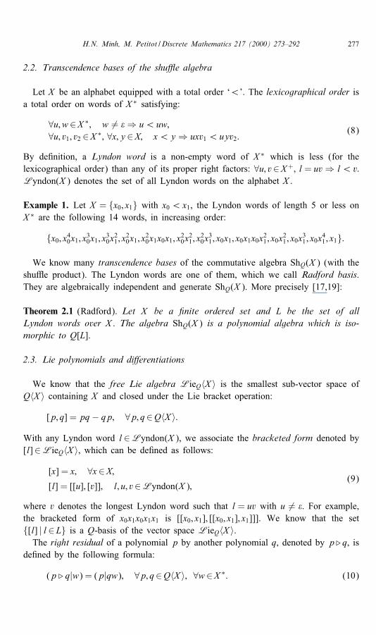
2.2. Transcendence bases of the shu�e algebra

Let X be an alphabet equipped with a total order ‘¡’. The lexicographical order isa total order on words of X ∗ satisfying:

∀u; w∈X ∗; w 6= �⇒ u¡uw;∀u; v1; v2 ∈X ∗; ∀x; y∈X; x¡y ⇒ uxv1¡uyv2:

(8)

By de�nition, a Lyndon word is a non-empty word of X ∗ which is less (for thelexicographical order) than any of its proper right factors: ∀u; v∈X+; l= uv⇒ l¡v:Lyndon(X ) denotes the set of all Lyndon words on the alphabet X .

Example 1. Let X = {x0; x1} with x0¡x1, the Lyndon words of length 5 or less onX ∗ are the following 14 words, in increasing order:

{x0; x40x1; x30x1; x30x21 ; x20x1; x20x1x0x1; x20x21 ; x20x31 ; x0x1; x0x1x0x21 ; x0x21 ; x0x31 ; x0x41 ; x1}:

We know many transcendence bases of the commutative algebra ShQ(X ) (with theshu�e product). The Lyndon words are one of them, which we call Radford basis.They are algebraically independent and generate ShQ(X ). More precisely [17,19]:

Theorem 2.1 (Radford). Let X be a �nite ordered set and L be the set of allLyndon words over X . The algebra ShQ(X ) is a polynomial algebra which is iso-morphic to Q[L].

2.3. Lie polynomials and di�erentiations

We know that the free Lie algebra LieQ〈X 〉 is the smallest sub-vector space ofQ〈X 〉 containing X and closed under the Lie bracket operation:

[p; q] = pq− qp; ∀p; q∈Q〈X 〉:

With any Lyndon word l∈Lyndon(X ), we associate the bracketed form denoted by[l]∈LieQ〈X 〉, which can be de�ned as follows:

[x] = x; ∀x∈X;[l] = [[u]; [v]]; l; u; v∈Lyndon(X );

(9)

where v denotes the longest Lyndon word such that l = uv with u 6= �. For example,the bracketed form of x0x1x0x1x1 is [[x0; x1]; [[x0; x1]; x1]]]. We know that the set{[l] | l∈L} is a Q-basis of the vector space LieQ〈X 〉.The right residual of a polynomial p by another polynomial q, denoted by p. q, is

de�ned by the following formula:

(p . q|w) = (p|qw); ∀p; q∈Q〈X 〉; ∀w∈X ∗: (10)

278 H.N. Minh, M. Petitot / Discrete Mathematics 217 (2000) 273–292

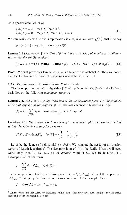
As a special case, we have

(xw) . x = w; ∀x∈X; ∀w∈X ∗;(xw) . y = 0; ∀x; y∈X; ∀w∈X ∗; x 6= y: (11)

We can easily check that this simpli�cation is a right action over Q〈X 〉, that is to sayp . (qr) = (p . q) . r; ∀p; q; r ∈Q〈X 〉:

Lemma 2.1 (Reutenauer [19]). The right residual by a Lie polynomial is a di�eren-tiation for the shu�e product:

(f g) . p= (f . p) g+ f (g . p); ∀f; g∈Q〈X 〉; ∀p∈LieQ〈X 〉: (12)

Proof. We �rst prove this lemma when p is a letter of the alphabet X . Then we noticethat the Lie bracket of two di�erentiations is a di�erentiation.

2.3.1. Decomposition algorithm in the Radford basisThe decomposition xtaylor algorithm [16] of a polynomial f∈Q〈X 〉 in the Radford

basis lies on the following triangular property:

Lemma 2.2. Let l be a Lyndon word and [l] be its bracketed form. l is the smallestword that appears in the support of [l]; and has coe�cient 1; that is to say:

[l] = l+∑w∈X ∗

�ww with |w|= |l|; w¿ l; �w ∈Z:

Corollary 2.1. The Lyndon words; according to the lexicographical by length ordering 3;satisfy the following triangular property:

∀l; l′ ∈Lyndon(X ); l . [l′] ={1 if l= l′;0 if l¡ l′:

(13)

Let d be the degree of polynomial f∈Q〈X 〉. We compute the set Ld of all Lyndonwords of length less than d. The decomposition of f in the Radford basis will needwords only from Ld. Let lmax be the greatest word of Ld. We are looking for adecomposition of the form

f =n∑i=0

Ai l imax; Ai ∈Q〈X 〉:

The decomposition of all Ai will take place in L′d=Ld \{lmax}, without the appearenceof lmax. To simplify the discussion, let us choose n= 2 for example. From

f = A2 l 2max + A1 lmax + A0;

3 Lyndon words are �rst sorted by increasing length, then, when they have equal lengths, they are sortedaccording to the lexicographical order.

H.N. Minh, M. Petitot / Discrete Mathematics 217 (2000) 273–292 279

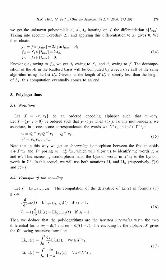
we get the unknown polynomials A0; A1; A2 iterating on f the di�erentiation .[lmax].Taking into account Corollary 2.1 and applying this di�erentiation to Ai gives 0. Wethen obtain:

f1 = f . [lmax] = 2A2 lmax + A1;f2 = f1 . [lmax] = 2A2;f3 = f2 . [lmax] = 0:

(14)

Knowing A2 owing to f2, we get A1 owing to f1, and A0 owing to f. The decompo-sition of the Ai in the Radford basis will be computed by a recursive call of the samealgorithm using the list L′d. Given that the length of L

′d is strictly less than the length

of Ld, this computation eventually comes to an end.

3. Polylogarithms

3.1. Notations

Let X = {x0; x1} be an ordered encoding alphabet such that x0¡x1.Let Y ={yi | i¿ 0} be ordered such that yi ¡yj when i¿ j. To any multi-index s, weassociate, in a one-to-one correspondence, the words w∈X ∗x1 and w′ ∈Y ∗ \ �:

w = xs1−10 x1xs2−10 x1 · · · xsk−10 x1;

w′ = ys1ys2 : : : ysk :(15)

Note that in this way we get an increasing isomorphism between the free monoids� + X ∗x1 and Y ∗ posing yi = xi−10 x1; which will allow us to identify the words s; wand w′. This increasing isomorphism maps the Lyndon words in X ∗x1 to the Lyndonwords in Y+. In this sequel, we will use both notations Lis and Liw (respectively, �(s)and �(w)).

3.2. Principle of the encoding

Let s = (s1; s2; : : : ; sk). The computation of the derivative of Lis(t) in formula (1)gives

tddtLis(t) = Li(s1−1;s2 ;:::;sk )(t) if s1¿ 1;

(1− t) ddtLis(t) = Li(s2 ;:::;sk )(t) if s1 = 1:

(16)

Then we deduce that the polylogarithms are the iterated integrales w.r.t. the twodi�erential forms !0 = dt=t and !1 = dt=(1− t). The encoding by the alphabet X givesthe following recursive formulae:

Lix0w(t) =∫ t

0

dzzLiw(z); ∀w∈X ∗x1;

Lix1w(t) =∫ t

0

dz1− zLiw(z); ∀w∈X ∗x1:

(17)

280 H.N. Minh, M. Petitot / Discrete Mathematics 217 (2000) 273–292

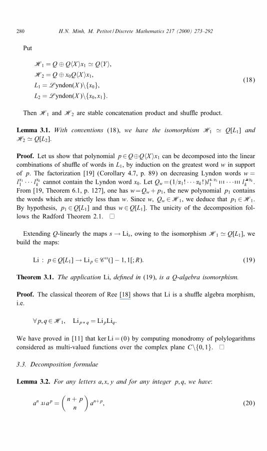
Put

H1 = Q ⊕ Q〈X 〉x1 ' Q〈Y 〉;H2 = Q ⊕ x0Q〈X 〉x1;L1 =Lyndon(X )\{x0};L2 =Lyndon(X )\{x0; x1}:

(18)

Then H1 and H2 are stable concatenation product and shu�e product.

Lemma 3.1. With conventions (18); we have the isomorphism H1 ' Q[L1] andH2 ' Q[L2].

Proof. Let us show that polynomial p∈Q⊕Q〈X 〉x1 can be decomposed into the linearcombinations of shu�e of words in L1, by induction on the greatest word w in supportof p. The factorization [19] (Corollary 4:7, p. 89) on decreasing Lyndon words w =l�11 · · · l�kk cannot contain the Lyndon word x0. Let Qw=(1=�1! · · · �k !)l �1

1 · · · l �kk .

From [19, Theorem 6:1, p. 127], one has w=Qw+p1, the new polynomial p1 containsthe words which are strictly less than w. Since w; Qw ∈H1, we deduce that p1 ∈H1.By hypothesis, p1 ∈Q[L1] and thus w∈Q[L1]. The unicity of the decomposition fol-lows the Radford Theorem 2.1.

Extending Q-linearly the maps s→ Lis, owing to the isomorphism H1 ' Q[L1], webuild the maps:

Li : p∈Q[L1]→ Lip ∈C!(]− 1; 1[;R): (19)

Theorem 3.1. The application Li; de�ned in (19); is a Q-algebra isomorphism.

Proof. The classical theorem of Ree [18] shows that Li is a shu�e algebra morphism,i.e.

∀p; q∈H1; Lip q = LipLiq:

We have proved in [11] that ker Li = (0) by computing monodromy of polylogarithmsconsidered as multi-valued functions over the complex plane C\{0; 1}.

3.3. Decomposition formulae

Lemma 3.2. For any letters a; x; y and for any integer p; q; we have:

an ap =(n+ pn

)an+p; (20)

H.N. Minh, M. Petitot / Discrete Mathematics 217 (2000) 273–292 281

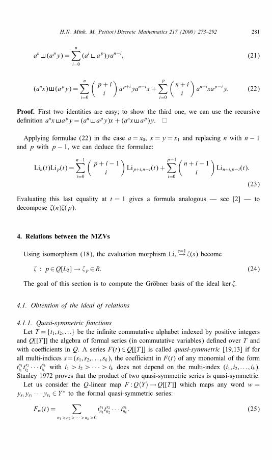
an (apy) =n∑i=0

(ai ap)yan−i ; (21)

(anx) (apy) =n∑i=0

(p+ ii

)ap+iyan−ix +

p∑i=0

(n+ ii

)an+ixap−iy: (22)

Proof. First two identities are easy; to show the third one, we can use the recursivede�nition anx apy = (an apy)x + (anx ap)y.

Applying formulae (22) in the case a = x0; x = y = x1 and replacing n with n − 1and p with p− 1, we can deduce the formulae:

Lin(t)Lip(t) =n−1∑i=0

(p+ i − 1

i

)Lip+i; n−i(t) +

p−1∑i=0

(n+ i − 1

i

)Lin+i;p−i(t):

(23)

Evaluating this last equality at t = 1 gives a formula analogous — see [2] — todecompose �(n)�(p).

4. Relations between the MZVs

Using isomorphism (18), the evaluation morphism Lisz=1→ �(s) become

� : p∈Q[L2]→ �p ∈R: (24)

The goal of this section is to compute the Gr�obner basis of the ideal ker �.

4.1. Obtention of the ideal of relations

4.1.1. Quasi-symmetric functionsLet T = {t1; t2; : : :} be the in�nite commutative alphabet indexed by positive integers

and Q[[T ]] the algebra of formal series (in commutative variables) de�ned over T andwith coe�cients in Q. A series F(t)∈Q[[T ]] is called quasi-symmetric [19,13] if forall multi-indices s=(s1; s2; : : : ; sk), the coe�cient in F(t) of any monomial of the formts1i1 t

s2i2 · · · tskik with i1¿i2¿ · · ·¿ik does not depend on the multi-index (i1; i2; : : : ; ik).

Stanley 1972 proves that the product of two quasi-symmetric series is quasi-symmetric.Let us consider the Q-linear map F :Q〈Y 〉→Q[[T ]] which maps any word w =

ys1ys2 · · ·ysk ∈Y ∗ to the formal quasi-symmetric series:

Fw(t) =∑

n1¿n2¿···¿nk¿0ts1n1 t

s2n2 · · · tsknk : (25)

282 H.N. Minh, M. Petitot / Discrete Mathematics 217 (2000) 273–292

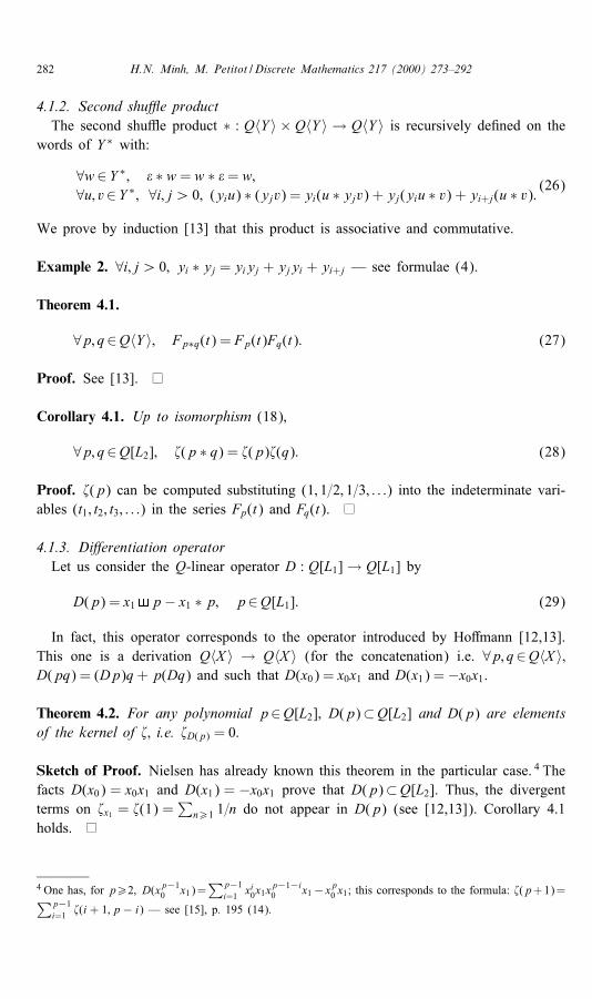
4.1.2. Second shu�e productThe second shu�e product ∗ : Q〈Y 〉 × Q〈Y 〉 → Q〈Y 〉 is recursively de�ned on the

words of Y ∗ with:

∀w∈Y ∗; � ∗ w = w ∗ �= w;∀u; v∈Y ∗; ∀i; j ¿ 0; (yiu) ∗ (yjv) = yi(u ∗ yjv) + yj(yiu ∗ v) + yi+j(u ∗ v): (26)

We prove by induction [13] that this product is associative and commutative.

Example 2. ∀i; j ¿ 0; yi ∗ yj = yiyj + yjyi + yi+j — see formulae (4).

Theorem 4.1.

∀p; q∈Q〈Y 〉; Fp∗q(t) = Fp(t)Fq(t): (27)

Proof. See [13].

Corollary 4.1. Up to isomorphism (18);

∀p; q∈Q[L2]; �(p ∗ q) = �(p)�(q): (28)

Proof. �(p) can be computed substituting (1; 1=2; 1=3; : : :) into the indeterminate vari-ables (t1; t2; t3; : : :) in the series Fp(t) and Fq(t).

4.1.3. Di�erentiation operatorLet us consider the Q-linear operator D : Q[L1]→ Q[L1] by

D(p) = x1 p− x1 ∗ p; p∈Q[L1]: (29)

In fact, this operator corresponds to the operator introduced by Ho�mann [12,13].This one is a derivation Q〈X 〉 → Q〈X 〉 (for the concatenation) i.e. ∀p; q∈Q〈X 〉;D(pq) = (Dp)q+ p(Dq) and such that D(x0) = x0x1 and D(x1) =−x0x1.

Theorem 4.2. For any polynomial p∈Q[L2]; D(p)⊂Q[L2] and D(p) are elementsof the kernel of �; i.e. �D(p) = 0:

Sketch of Proof. Nielsen has already known this theorem in the particular case. 4 Thefacts D(x0) = x0x1 and D(x1) = −x0x1 prove that D(p)⊂Q[L2]. Thus, the divergentterms on �x1 = �(1) =

∑n¿1 1=n do not appear in D(p) (see [12,13]). Corollary 4.1

holds.

4 One has, for p¿2; D(xp−10 x1)=∑p−1

i=1xi0x1x

p−1−i0 x1− xp0 x1; this corresponds to the formula: �(p+1)=∑p−1

i=1�(i + 1; p− i) — see [15], p. 195 (14).

H.N. Minh, M. Petitot / Discrete Mathematics 217 (2000) 273–292 283

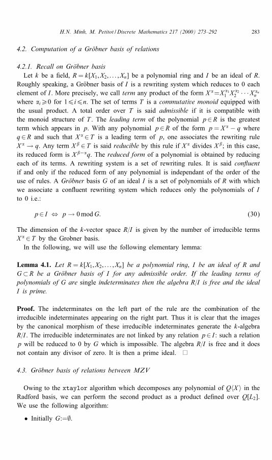
4.2. Computation of a Gr�obner basis of relations

4.2.1. Recall on Gr�obner basisLet k be a �eld, R= k[X1; X2; : : : ; Xn] be a polynomial ring and I be an ideal of R.

Roughly speaking, a Gr�obner basis of I is a rewriting system which reduces to 0 eachelement of I . More precisely, we call term any product of the form X �=X �11 X

�22 · · ·X �nn

where �i¿0 for 16i6n. The set of terms T is a commutative monoid equipped withthe usual product. A total order over T is said admissible if it is compatible withthe monoid structure of T . The leading term of the polynomial p∈R is the greatestterm which appears in p. With any polynomial p∈R of the form p = X � − q whereq∈R and such that X � ∈T is a leading term of p, one associates the rewriting ruleX � → q. Any term X � ∈T is said reducible by this rule if X � divides X �; in this case,its reduced form is X �−�q. The reduced form of a polynomial is obtained by reducingeach of its terms. A rewriting system is a set of rewriting rules. It is said con uentif and only if the reduced form of any polynomial is independant of the order of theuse of rules. A Gr�obner basis G of an ideal I is a set of polynomials of R with whichwe associate a con uent rewriting system which reduces only the polynomials of Ito 0 i.e.:

p∈ I ⇔ p→ 0modG: (30)

The dimension of the k-vector space R=I is given by the number of irreducible termsX � ∈T by the Grobner basis.In the following, we will use the following elementary lemma:

Lemma 4.1. Let R = k[X1; X2; : : : ; Xn] be a polynomial ring; I be an ideal of R andG⊂R be a Gr�obner basis of I for any admissible order. If the leading terms ofpolynomials of G are single indeterminates then the algebra R=I is free and the idealI is prime.

Proof. The indeterminates on the left part of the rule are the combination of theirreducible indeterminates appearing on the right part. Thus it is clear that the imagesby the canonical morphism of these irreducible indeterminates generate the k-algebraR=I . The irreducible indeterminates are not linked by any relation p∈ I : such a relationp will be reduced to 0 by G which is impossible. The algebra R=I is free and it doesnot contain any divisor of zero. It is then a prime ideal.

4.3. Gr�obner basis of relations between MZV

Owing to the xtaylor algorithm which decomposes any polynomial of Q〈X 〉 in theRadford basis, we can perform the second product as a product de�ned over Q[L2].We use the following algorithm:

• Initially G:=∅.

284 H.N. Minh, M. Petitot / Discrete Mathematics 217 (2000) 273–292

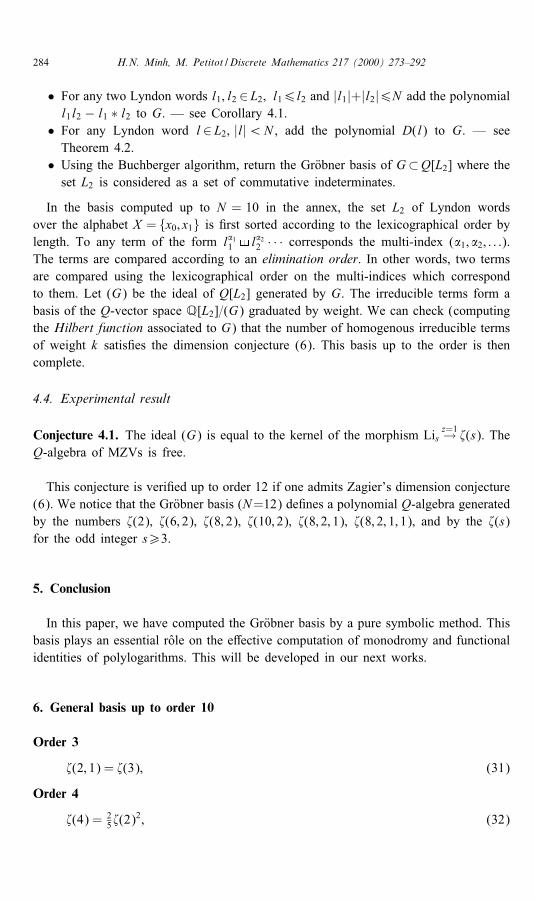
• For any two Lyndon words l1; l2 ∈L2; l16l2 and |l1|+|l2|6N add the polynomiall1l2 − l1 ∗ l2 to G. — see Corollary 4.1.

• For any Lyndon word l∈L2; |l|¡N , add the polynomial D(l) to G. — seeTheorem 4.2.

• Using the Buchberger algorithm, return the Gr�obner basis of G⊂Q[L2] where theset L2 is considered as a set of commutative indeterminates.

In the basis computed up to N = 10 in the annex, the set L2 of Lyndon wordsover the alphabet X = {x0; x1} is �rst sorted according to the lexicographical order bylength. To any term of the form l�11 l�22 · · · corresponds the multi-index (�1; �2; : : :).The terms are compared according to an elimination order. In other words, two termsare compared using the lexicographical order on the multi-indices which correspondto them. Let (G) be the ideal of Q[L2] generated by G. The irreducible terms form abasis of the Q-vector space Q[L2]=(G) graduated by weight. We can check (computingthe Hilbert function associated to G) that the number of homogenous irreducible termsof weight k satis�es the dimension conjecture (6). This basis up to the order is thencomplete.

4.4. Experimental result

Conjecture 4.1. The ideal (G) is equal to the kernel of the morphism Lisz=1→ �(s). The

Q-algebra of MZVs is free.

This conjecture is veri�ed up to order 12 if one admits Zagier’s dimension conjecture(6). We notice that the Gr�obner basis (N=12) de�nes a polynomial Q-algebra generatedby the numbers �(2); �(6; 2); �(8; 2); �(10; 2); �(8; 2; 1); �(8; 2; 1; 1); and by the �(s)for the odd integer s¿3.

5. Conclusion

In this paper, we have computed the Gr�obner basis by a pure symbolic method. Thisbasis plays an essential role on the e�ective computation of monodromy and functionalidentities of polylogarithms. This will be developed in our next works.

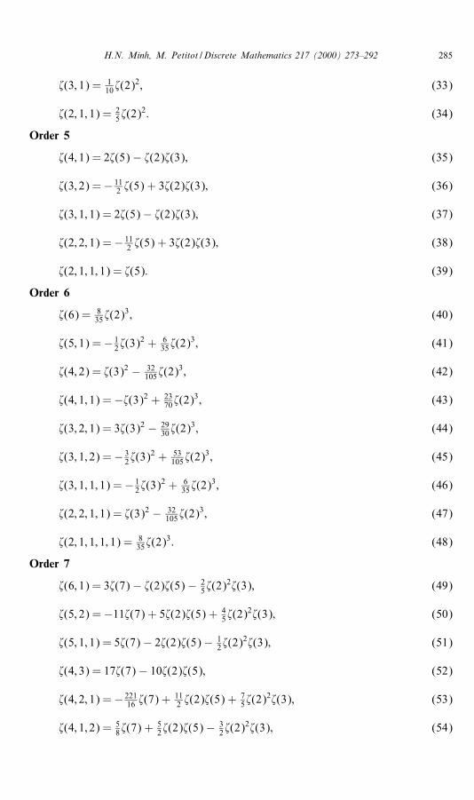
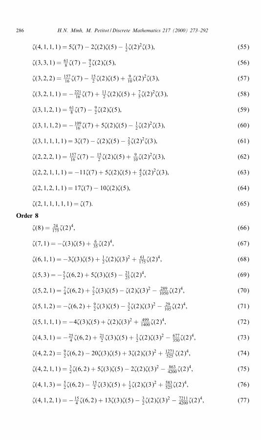
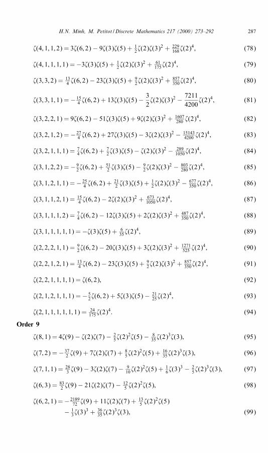
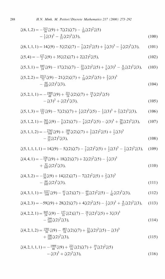
6. General basis up to order 10

Order 3

�(2; 1) = �(3); (31)

Order 4

�(4) = 25�(2)

2; (32)

H.N. Minh, M. Petitot / Discrete Mathematics 217 (2000) 273–292 285

�(3; 1) = 110�(2)

2; (33)

�(2; 1; 1) = 25�(2)

2: (34)

Order 5

�(4; 1) = 2�(5)− �(2)�(3); (35)

�(3; 2) =− 112 �(5) + 3�(2)�(3); (36)

�(3; 1; 1) = 2�(5)− �(2)�(3); (37)

�(2; 2; 1) =− 112 �(5) + 3�(2)�(3); (38)

�(2; 1; 1; 1) = �(5): (39)

Order 6

�(6) = 835�(2)

3; (40)

�(5; 1) =− 12�(3)

2 + 635�(2)

3; (41)

�(4; 2) = �(3)2 − 32105�(2)

3; (42)

�(4; 1; 1) =−�(3)2 + 2370�(2)

3; (43)

�(3; 2; 1) = 3�(3)2 − 2930�(2)

3; (44)

�(3; 1; 2) =− 32�(3)

2 + 53105�(2)

3; (45)

�(3; 1; 1; 1) =− 12�(3)

2 + 635�(2)

3; (46)

�(2; 2; 1; 1) = �(3)2 − 32105�(2)

3; (47)

�(2; 1; 1; 1; 1) = 835�(2)

3: (48)

Order 7

�(6; 1) = 3�(7)− �(2)�(5)− 25�(2)

2�(3); (49)

�(5; 2) =−11�(7) + 5�(2)�(5) + 45�(2)

2�(3); (50)

�(5; 1; 1) = 5�(7)− 2�(2)�(5)− 12�(2)

2�(3); (51)

�(4; 3) = 17�(7)− 10�(2)�(5); (52)

�(4; 2; 1) =− 22116 �(7) +

112 �(2)�(5) +

75�(2)

2�(3); (53)

�(4; 1; 2) = 58�(7) +

52�(2)�(5)− 3

2�(2)2�(3); (54)

286 H.N. Minh, M. Petitot / Discrete Mathematics 217 (2000) 273–292

�(4; 1; 1; 1) = 5�(7)− 2�(2)�(5)− 12�(2)

2�(3); (55)

�(3; 3; 1) = 618 �(7)− 9

2�(2)�(5); (56)

�(3; 2; 2) = 15716 �(7)− 15

2 �(2)�(5) +910�(2)

2�(3); (57)

�(3; 2; 1; 1) =− 22116 �(7) +

112 �(2)�(5) +

75�(2)

2�(3); (58)

�(3; 1; 2; 1) = 618 �(7)− 9

2�(2)�(5); (59)

�(3; 1; 1; 2) =− 10916 �(7) + 5�(2)�(5)− 1

2�(2)2�(3); (60)

�(3; 1; 1; 1; 1) = 3�(7)− �(2)�(5)− 25�(2)

2�(3); (61)

�(2; 2; 2; 1) = 15716 �(7)− 15

2 �(2)�(5) +910�(2)

2�(3); (62)

�(2; 2; 1; 1; 1) =−11�(7) + 5�(2)�(5) + 45�(2)

2�(3); (63)

�(2; 1; 2; 1; 1) = 17�(7)− 10�(2)�(5); (64)

�(2; 1; 1; 1; 1; 1) = �(7): (65)

Order 8

�(8) = 24175�(2)

4; (66)

�(7; 1) =−�(3)�(5) + 635�(2)

4; (67)

�(6; 1; 1) =−3�(3)�(5) + 12�(2)�(3)

2 + 61175�(2)

4; (68)

�(5; 3) =− 52�(6; 2) + 5�(3)�(5)− 21

25�(2)4; (69)

�(5; 2; 1) = 74�(6; 2) +

72�(3)�(5)− �(2)�(3)2 − 289

1050�(2)4; (70)

�(5; 1; 2) =−�(6; 2) + 92�(3)�(5)− 3

2�(2)�(3)2 − 29

105�(2)4; (71)

�(5; 1; 1; 1) =−4�(3)�(5) + �(2)�(3)2 + 4991400�(2)

4; (72)

�(4; 3; 1) =− 254 �(6; 2) +

212 �(3)�(5) +

12�(2)�(3)

2 − 677350�(2)

4; (73)

�(4; 2; 2) = 92�(6; 2)− 20�(3)�(5) + 3�(2)�(3)2 + 1271

525 �(2)4; (74)

�(4; 2; 1; 1) = 32�(6; 2) + 5�(3)�(5)− 2�(2)�(3)2 − 863

4200�(2)4; (75)

�(4; 1; 3) = 52�(6; 2)− 15

2 �(3)�(5) +12�(2)�(3)

2 + 583525�(2)

4; (76)

�(4; 1; 2; 1) =− 154 �(6; 2) + 13�(3)�(5)− 3

2�(2)�(3)2 − 7211

4200�(2)4; (77)

H.N. Minh, M. Petitot / Discrete Mathematics 217 (2000) 273–292 287

�(4; 1; 1; 2) = 3�(6; 2)− 9�(3)�(5) + 12�(2)�(3)

2 + 229168�(2)

4; (78)

�(4; 1; 1; 1; 1) =−3�(3)�(5) + 12�(2)�(3)

2 + 61175�(2)

4; (79)

�(3; 3; 2) = 134 �(6; 2)− 23�(3)�(5) + 9

2�(2)�(3)2 + 857

350�(2)4; (80)

�(3; 3; 1; 1) =− 154 �(6; 2) + 13�(3)�(5)−

32�(2)�(3)2 − 7211

4200�(2)4; (81)

�(3; 2; 2; 1) = 9�(6; 2)− 51�(3)�(5) + 9�(2)�(3)2 + 1607280 �(2)

4; (82)

�(3; 2; 1; 2) =− 274 �(6; 2) + 27�(3)�(5)− 3�(2)�(3)2 − 15143

4200 �(2)4; (83)

�(3; 2; 1; 1; 1) = 74�(6; 2) +

72�(3)�(5)− �(2)�(3)2 − 289

1050�(2)4; (84)

�(3; 1; 2; 2) =− 92�(6; 2) +

512 �(3)�(5)− 9

2�(2)�(3)2 − 803

280�(2)4; (85)

�(3; 1; 2; 1; 1) =− 254 �(6; 2) +

212 �(3)�(5) +

12�(2)�(3)

2 − 677350�(2)

4; (86)

�(3; 1; 1; 2; 1) = 154 �(6; 2)− 2�(2)�(3)2 + 673

1050�(2)4; (87)

�(3; 1; 1; 1; 2) = 74�(6; 2)− 12�(3)�(5) + 2�(2)�(3)2 + 487

350�(2)4; (88)

�(3; 1; 1; 1; 1; 1) =−�(3)�(5) + 635�(2)

4; (89)

�(2; 2; 2; 1; 1) = 92�(6; 2)− 20�(3)�(5) + 3�(2)�(3)2 + 1271

525 �(2)4; (90)

�(2; 2; 1; 2; 1) = 134 �(6; 2)− 23�(3)�(5) + 9

2�(2)�(3)2 + 857

350�(2)4; (91)

�(2; 2; 1; 1; 1; 1) = �(6; 2); (92)

�(2; 1; 2; 1; 1; 1) =− 52�(6; 2) + 5�(3)�(5)− 21

25�(2)4; (93)

�(2; 1; 1; 1; 1; 1; 1) = 24175�(2)

4: (94)

Order 9

�(8; 1) = 4�(9)− �(2)�(7)− 25�(2)

2�(5)− 835�(2)

3�(3); (95)

�(7; 2) =− 372 �(9) + 7�(2)�(7) +

85�(2)

2�(5) + 1635�(2)

3�(3); (96)

�(7; 1; 1) = 283 �(9)− 3�(2)�(7)− 9

10�(2)2�(5) + 1

6�(3)3 − 2

5�(2)3�(3); (97)

�(6; 3) = 832 �(9)− 21�(2)�(7)− 12

5 �(2)2�(5); (98)

�(6; 2; 1) =− 218972 �(9) + 11�(2)�(7) +

135 �(2)

2�(5)

− 13�(3)

3 + 3635�(2)

3�(3); (99)

288 H.N. Minh, M. Petitot / Discrete Mathematics 217 (2000) 273–292

�(6; 1; 2) =− 31336 �(9) + 7�(2)�(7)− 1

10�(2)2�(5)

− 13�(3)

3 − 821�(2)

3�(3); (100)

�(6; 1; 1; 1) = 14�(9)− 5�(2)�(7)− 75�(2)

2�(5) + 12�(3)

3 − 12�(2)

3�(3); (101)

�(5; 4) =− 1272 �(9) + 35�(2)�(7) + 2�(2)

2�(5); (102)

�(5; 3; 1) = 84524 �(9)− 17�(2)�(7)− 23

10�(2)2�(5) + 1

6�(3)3 − 6

35�(2)3�(3); (103)

�(5; 2; 2) = 251372 �(9)− 21�(2)�(7) + 7

10�(2)2�(5) + 2

3�(3)3

− 64105�(2)

3�(3); (104)

�(5; 2; 1; 1) =− 190948 �(9) +

22116 �(2)�(7) +

194 �(2)

2�(5)

− �(3)3 + �(2)3�(3); (105)

�(5; 1; 3) = 12112 �(9)− 7�(2)�(7) + 1

5�(2)2�(5)− 1

3�(3)3 + 2

7�(2)3�(3); (106)

�(5; 1; 2; 1) = 361144�(9)− 5

8�(2)�(7)− 74�(2)

2�(5)− �(3)3 + 2930�(2)

3�(3); (107)

�(5; 1; 1; 2) =− 2765144 �(9) +

18916 �(2)�(7) +

35�(2)

2�(5) + 12�(3)

3

− 1935�(2)

3�(3); (108)

�(5; 1; 1; 1; 1) = 14�(9)− 5�(2)�(7)− 75�(2)

2�(5) + 12�(3)

3 − 12�(2)

3�(3); (109)

�(4; 4; 1) =− 3289 �(9) + 18�(2)�(7) + 2�(2)

2�(5)− 13�(3)

3

+ 32105�(2)

3�(3); (110)

�(4; 3; 2) =− 5336�(9) + 14�(2)�(7)− 7�(2)2�(5) + 2

3�(3)3

− 64105�(2)

3�(3); (111)

�(4; 3; 1; 1) = 3227144 �(9)− 61

8 �(2)�(7)− 6920�(2)

2�(5)− 142�(2)

3�(3); (112)

�(4; 2; 3) =−59�(9) + 28�(2)�(7) + 4�(2)2�(5)− 13�(3)

3 + 821�(2)

3�(3); (113)

�(4; 2; 2; 1) = 84524 �(9)− 157

16 �(2)�(7)− 165 �(2)

2�(5) + 3�(3)3

− 299105�(2)

3�(3); (114)

�(4; 2; 1; 2) = 150136 �(9)− 483

16 �(2)�(7) +3320�(2)

2�(5)− �(3)3+ 106

105�(2)3�(3); (115)

�(4; 2; 1; 1; 1) =− 190948 �(9) +

22116 �(2)�(7) +

194 �(2)

2�(5)

− �(3)3 + �(2)3�(3); (116)

H.N. Minh, M. Petitot / Discrete Mathematics 217 (2000) 273–292 289

�(4; 1; 3; 1) = 103144�(9) +

14�(2)�(7) +

14�(2)

2�(5) + 12�(3)

3

− 53105�(2)

3�(3); (117)

�(4; 1; 2; 2) =− 118736 �(9) +

18916 �(2)�(7) +

154 �(2)

2�(5)− �(3)3+ 61

70�(2)3�(3); (118)

�(4; 1; 2; 1; 1) = 3227144 �(9)− 61

8 �(2)�(7)− 6920�(2)

2�(5)− 142�(2)

3�(3); (119)

�(4; 1; 1; 3) = 3721144 �(9)− 231

16 �(2)�(7)− �(2)2�(5)− 12�(3)

3

+ 34105�(2)

3�(3); (120)

�(4; 1; 1; 2; 1) =− 4067144 �(9) +

10916 �(2)�(7) +

4310�(2)

2�(5)− 32�(3)

3

+ 148105�(2)

3�(3); (121)

�(4; 1; 1; 1; 2) = 265144�(9) + 7�(2)�(7)− 13

5 �(2)2�(5) + 3

2�(3)3

− 172105�(2)

3�(3); (122)

�(4; 1; 1; 1; 1; 1) = 283 �(9)− 3�(2)�(7)− 9

10�(2)2�(5) + 1

6�(3)3

− 25�(2)

3�(3); (123)

�(3; 3; 2; 1) = 100936 �(9)− 75

8 �(2)�(7)− 920�(2)

2�(5) + 72�(3)

3

− 22770 �(2)

3�(3); (124)

�(3; 3; 1; 2) =− 120572 �(9) +

18916 �(2)�(7)− 27

20�(2)2�(5)− 1

2�(3)3

+ 1235�(2)

3�(3); (125)

�(3; 3; 1; 1; 1) = 361144�(9)− 5

8�(2)�(7)− 74�(2)

2�(5)− �(3)3 + 2930�(2)

3�(3); (126)

�(3; 2; 3; 1) =− 3678 �(9) +

29116 �(2)�(7)− 9

2�(3)3 + 309

70 �(2)3�(3); (127)

�(3; 2; 2; 2) =− 22316 �(9) +

18916 �(2)�(7)− 9

4�(2)2�(5) + 9

70�(2)3�(3); (128)

�(3; 2; 2; 1; 1) = 84524 �(9)− 157

16 �(2)�(7)− 165 �(2)

2�(5) + 3�(3)3

− 299105�(2)

3�(3); (129)

�(3; 2; 1; 2; 1) = 100936 �(9)− 75

8 �(2)�(7)− 920�(2)

2�(5) + 72�(3)

3

− 22770 �(2)

3�(3); (130)

�(3; 2; 1; 1; 2) = 98972 �(9)− 21�(2)�(7) + 33

20�(2)2�(5)− 4�(3)3

+ 15335 �(2)

3�(3); (131)

�(3; 2; 1; 1; 1; 1) =− 218972 �(9) + 11�(2)�(7) +

135 �(2)

2�(5)− 13�(3)

3

+ 3635�(2)

3�(3); (132)

290 H.N. Minh, M. Petitot / Discrete Mathematics 217 (2000) 273–292

�(3; 1; 3; 1; 1) = 103144�(9) +

14�(2)�(7) +

14�(2)

2�(5) + 12�(3)

3

− 53105�(2)

3�(3); (133)

�(3; 1; 2; 2; 1) =− 3678 �(9) +

29116 �(2)�(7)− 9

2�(3)3 + 309

70 �(2)3�(3); (134)

�(3; 1; 2; 1; 2) =− 916 �(9) + 14�(2)�(7)− 9

10�(2)2�(5) + 3

2�(3)3

− 5335�(2)

3�(3); (135)

�(3; 1; 2; 1; 1; 1) = 84524 �(9)− 17�(2)�(7)− 23

10�(2)2�(5) + 1

6�(3)3

− 635�(2)

3�(3); (136)

�(3; 1; 1; 2; 2) = 80336 �(9)− 14�(2)�(7) + 17

10�(2)2�(5) + �(3)3

− 221210�(2)

3�(3); (137)

�(3; 1; 1; 2; 1; 1) =− 3289 �(9) + 18�(2)�(7) + 2�(2)

2�(5)− 13�(3)

3

+ 32105�(2)

3�(3); (138)

�(3; 1; 1; 1; 2; 1) = 34124 �(9)− 10�(2)�(7) + 1

2�(2)2�(5)− 1

3�(3)3

+ 27�(2)

3�(3); (139)

�(3; 1; 1; 1; 1; 2) =− 46172 �(9) + 7�(2)�(7)− 7

10�(2)2�(5) + 2

3�(3)3

− 86105�(2)

3�(3); (140)

�(3; 1; 1; 1; 1; 1; 1) = 4�(9)− �(2)�(7)− 25�(2)

2�(5)− 835�(2)

3�(3); (141)

�(2; 2; 2; 2; 1) =− 22316 �(9) +

18916 �(2)�(7)− 9

4�(2)2�(5) + 9

70�(2)3�(3); (142)

�(2; 2; 2; 1; 1; 1) = 251372 �(9)− 21�(2)�(7) + 7

10�(2)2�(5) + 2

3�(3)3

− 64105�(2)

3�(3); (143)

�(2; 2; 1; 2; 1; 1) =− 5336�(9) + 14�(2)�(7)− 7�(2)2�(5) + 2

3�(3)3

− 64105�(2)

3�(3); (144)

�(2; 2; 1; 1; 2; 1) = 59336 �(9)− 14�(2)�(7) + 3�(2)2�(5) + 2

3�(3)3

− 815�(2)

3�(3); (145)

�(2; 2; 1; 1; 1; 1; 1) =− 372 �(9) + 7�(2)�(7) +

85�(2)

2�(5) + 1635�(2)

3�(3); (146)

�(2; 1; 2; 1; 1; 1; 1) = 832 �(9)− 21�(2)�(7)− 12

5 �(2)2�(5); (147)

�(2; 1; 1; 2; 1; 1; 1) =− 1272 �(9) + 35�(2)�(7) + 2�(2)

2�(5); (148)

�(2; 1; 1; 1; 1; 1; 1; 1) = �(9): (149)

H.N. Minh, M. Petitot / Discrete Mathematics 217 (2000) 273–292 291

Order 10

�(10) = 32385�(2)

5; (150)

�(9; 1) =−�(3)�(7)− 12�(5)

2 + 855�(2)

5; (151)

�(8; 1; 1) =−4�(3)�(7)− 2�(5)2 + �(2)�(3)�(5) + 15�(2)

2�(3)2

+ 6661925�(2)

5; (152)

�(7; 3) =− 72�(8; 2) + 7�(3)�(7) + 4�(5)

2 − 408385�(2)

5; (153)

�(7; 2; 1) = 94�(8; 2)− �(2)�(6; 2) + 9

2�(3)�(7) +94�(5)

2

− 25�(2)

2�(3)2 − 30165775�(2)

5; (154)

�(7; 1; 2) =−�(8; 2) + �(2)�(6; 2) + 10�(3)�(7) + 5�(5)2 − 7�(2)�(3)�(5)− 2

5�(2)2�(3)2 − 2

15�(2)5; (155)

�(7; 1; 1; 1) =−8�(3)�(7)− 4�(5)2 + 3�(2)�(3)�(5) + 920�(2)

2�(3)2

+ 139275�(2)

5; (156)

�(6; 4) = 72�(8; 2)− 7�(3)�(7)− 5�(5)2 + 2216

1925�(2)5; (157)

...

�(2; 1; 1; 2; 1; 1; 1; 1) = 72�(8; 2)− 7�(3)�(7)− 5�(5)2 + 2216

1925�(2)5; (158)

�(2; 1; 1; 1; 1; 1; 1; 1; 1) = 32385�(2)

5: (159)

Acknowledgements

We thank Ph. Flajolet, J. Borwein and M. Ho�man for having communicated theirpapers to us, thus encouraging us in the pursuit of this study. The Gr�obner basis hasbeen veri�ed owing to the EZ-FACE piece of software, which J. Borwein has beenmade available on the WEB. We also thank to J. Marchand, system administrator forthe group Medicis in the GAGE lab, at the �Ecole Polytechnique in Palaiseau.

References

[1] V.I. Arnold, The Vassiliev theory of discriminants and knots, in: First European Congress ofMathematics, Vol. 1, Birkh�auser, Basel, 1994, pp. 3–29.

[2] D. Borwein, J.M. Borwein, R. Girgensohn, Explicit evaluation of Euler sums, Proc. Edinburgh Math.Soc. 38 (1995) 277–294.

292 H.N. Minh, M. Petitot / Discrete Mathematics 217 (2000) 273–292

[3] J.M. Borwein, D.M. Bradley, D.J. Broadhurst, Evaluation of k-fold Euler=Zagier sums: a compendiumof results for arbitrary k.

[4] J.M. Borwein, R. Girgensohn, Evaluation of triple Euler sums, Electron. J. Combin. 3 (1996) R23.[5] Ph. Flajolet, G. Labelle, L. Laforest, B. Salvy, Hypergeometrics and the cost structure of quadtree,

Random Struct. Algorithms 7 (1995) 117–143.[6] Ph. Flajolet, B. Salvy, Euler sums and contour integral representations, Exp. Math. 7 (1998) 15–35.[7] I.M. Guelfand, D. Krob, A. Lascoux, B. Leclerc, V.S. Retakh, J.Y. Thibon, Non-commutative symmetric

functions, Adv. in Math. 112 (1995) 218–348.[8] Minh Hoang Ngoc, Polylogarithms & evaluation transform, IMACS Symposium, Lille, June 1993.[9] Minh Hoang Ngoc, Int�egration symbolique des �equations di��erentielles lin�eaires, FPSAC’96,

Minneapolis, June 1996.[10] Minh Hoang Ngoc, Summations of polylogarithms via evaluation transform, Math. Comput. Simulation

1336 (1996) 707–728.[11] Minh Hoang Ngoc, M. Petitot, J. Van Der Hoeven, Shu�e algebra and polylogarithms, Proc. of

FPSAC’98, 10th International Conference on Formal Power Series and Algebraic Combinatorics,Toronto, June 1998.

[12] M. Ho�man, Multiple harmonic series, Paci�c J. Math. 152 (2) (1992) 275–290.[13] M. Ho�man, The algebra of multiple harmonic series, J. Algebra 194 (1997) 477–495.[14] C. Markett, Triple sums and the Riemann zeta function, J. Number Theory 48 (1994) 113–132.[15] N. Nielsen, Recherches sur le carr�e de la d�eriv�ee logarithmique de la fonction gamma et sur quelques

fonctions analogues, Annali di Matematica 9 (1904) 190–210.[16] M. Petitot, Alg�ebre non commutative en Scratchpad, Application au probl�eme de la r�ealisation minimale

analytique, Th�ese de Doctorat, Universit�e Lille I, Janvier, 1992.[17] D.E. Radford, A natural ring basis for the shu�e algebra and an application to group schemes,

J. Algebra 58 (1979) 432–454.[18] R. Ree, Lie elements and an algebra associated with shu�es, Ann. Math. 68 (1958) 210–220.[19] C. Reutenauer, Free Lie Algebras, London Mathematical Society Monographs, Vol. New Series-7,

Oxford Science Press Inc, New York, 1993.[20] D. Zagier, Values of zeta functions and their applications, in: First European Congress of Mathematics,

Vol. 2, Birkh�auser, Basel, 1994, pp. 497–512.