(5^: 731'so f - wur edepot
TRANSCRIPT

iu^o2?o\, £ ^ l o
Extending Generalized Linear Models with Random Effects and Components of Dispersion
Gegeneraliseerde Lineaire Modellen met Extra Stochastische Termen en Bijbehorende Variantiecomponenten
(5^: 731'so f

Promotoren: dr. D.A.M.K. Rasch hoogleraar in de wiskundige statistiek
dr. J.C. van Houwelingen hoogleraar in de medische statistiek Rijksuniversiteit Leiden

* H 4 Û 2 ? O < ( 2-2.IO
Bas Engel
Extending Generalized Linear Models with Random Effects and Components of Dispersion
Proefschrift ter verkrijging van de graad van doctor op gezag van de rector magnificus van de Landbouwuniversiteit Wageningen, dr. C.M. Karssen, in het openbaar te verdedigen op vrijdag 24 januari 1997 des middags te één uur dertig in de Aula.
lsngi(^ö(

Slftiji Tiiïtó-X
ISBN 90-5485-639-4

ffno2zo] x go)Q
Stellingen
Het is nog steeds mogelijk met reeds lang bestaande modellen en technieken tot grote besparing van onderzoekskosten te komen. Zo kunnen met een combinatie van lineaire regressie en "double sampling" bij de voorspelling van het vleespercentage van varkenskarkassen de experimentele kosten worden gehalveerd, zonder verlies van nauwkeurigheid van de schattingen van de regressiecoëffrciënten.
Engel, B., Walstra, P. (1991). Increasing precision or reducing expense in regression experiments by using information from a concomitant variable. Biometrics 47, 13-20.
Engel, B., Walstra, P. (1991). A simple method to increase precision or reduce expense in regression experiments to predict the proportion of lean meat of carcasses. Animal Production 53, 353-359.
Het gebruik van een drempelmodel waarin een onderliggende variabele een "animal model" volgt, en analyse van de data volgens de methoden beschreven in Hoofdstuk 7 van dit proefschrift, leiden tot een efficiency verhoging met betrekking tot de genetische vooruitgang van 1 a 2 % ten opzichte van analyse met een conventioneel animal model voor normaal verdeelde data. Dit is slechts een kleine winst, maar wanneer de beste stieren selectief worden ingezet op de beste bedrijven, stijgt de winst tot 7 tot 20 %. Daarmee is aangetoond dat gebruik van het statistisch veel verantwoorder drempelmodel, ook voor grote data sets en voor resultaten op populatieniveau, in alle opzichten aantrekkelijk is.
Meuwissen, T.H.E., Engel, B., van der Werf, J.H.J. (1995). Maximizing selection efficiency for categorical traits. Journal of Animal Science 73, 1933-1939.
De Gibbs sampler produceert resultaten waar andere statistische technieken vanwege numerieke beperkingen falen. Onderzoekers omarmen tegelijk met dit algorithme schijnbaar probleemloos de bijbehorende Bayesiaanse filosofie. Binnen het statistiek onderwijs dient het onderscheid tussen frequentistische en Bayesiaanse beschouwingen scherper naar voren te worden gebracht opdat een meer bewuste keuze kan worden gemaakt.
Het gebruik van vertrouwde technieken, waar zij strikt genomen niet van toepassing zijn (denk aan variantieanalyse op discrete data), wordt vaak gerechtvaardigd met de opmerking dat "het meestal toch niet veel uitmaakt". Dit is de dood in de pot voor de ontwikkeling van nieuwe statistische modellen, die genuanceerdere conclusies toelaten.
Random effecten kunnen een veel grotere rol binnen de toegepaste statistiek spelen dan thans het geval is. Random effecten maken het mogelijk om grote aantallen parameters op stabiele wijze in een model op te nemen. Gelijkenis tussen experimentele eenheden kan worden weergegeven met behulp van een beperkt aantal variantiecomponenten.
De benaming "improper" voor niet-informatieve a priori verdelingen kan met recht met "onfatsoenlijk" vertaald worden: hier worden de regels van het probabilistisch fatsoen ruimschoots overschreden.
7. Een statisticus is niet objectief. Maar een goede statisticus probeert het, altijd weer opnieuw, wel te zijn.

Elk model is een karikatuur van de werkelijkheid. De grove lijnen zijn aanwezig, maar de details ontbreken. Er is geen enkele garantie dat de conclusies ontleend aan berekeningen binnen het model, relevant zijn voor de werkelijkheid. De enige rechtvaardiging is het succes bij gebruik voor praktijkproblemen. Daar er vaak geen alternatieven voor handen zijn, anders dan het blind nemen van besluiten, is succes al gauw verzekerd. Dit noopt op zijn minst tot bescheidenheid en voorzichtigheid.
Geld speelt geen rol zou heer Olivier B. Bommel zeggen. Dat geldt helaas niet voor de verzamelaars van het werk van Marten Toonder. Mede als gevolg van de adviesprijzen in de Bommelbibliografie van H. Matla (uitgeverij en antiquariaat Panda, Den Haag) liegen de prijzen voor bommeldingen er niet om. De Marten Toonder Verzamelaars Club zou zich de nobele taak moeten stellen om dit opgeschroefde prijsniveau te doorbreken: betaalbare facsimile uitgaves in eigen beheer zouden het vroege werk van Toonder weer binnen bereik van de oplettende lezertjes brengen.
10. Zeker in een tijd waar kinderen op school steeds meer moeten leren, mag vereenvoudiging van de spelling niet langer een punt van discussie zijn. De taal is in de eerste plaats een communicatiemiddel. Historische en culturele argumenten zijn hieraan ondergeschikt.
De thans nog experimentele wachttijdindicator bij stoplichten voor fietsers dient groot genoeg te zijn om in het voorbijgaan te kunnen worden afgelezen.
12. De wetenschap gaat aan management ten onder.
13. "De uitvreter" (de Gids, 1911) en "Titaantjes" (Groot Nederland, 1915) van Nescio (pseudoniem van J.H.F. Grönloh, 1881-1961) behoren tot de mooiste literatuur die in de Nederlandse taal is voortgebracht.
Stellingen behorende bij het proefschrift "Extending generalized linear models with random effects and components of dispersion" door Bas Engel, te verdedigen op 24 januari 1997 te Wageningen.

Voor Ineke
"Jelui kerels zijn zo akelig wijs: alles moet een reden en een doel hebben."
Nescio (J.H.F.Grónloh, 1881-1961), in "De uitvreter" (de Gids, 1911).

Voorwoord
Dit proefschrift is een bundeling van artikelen over gemengde modellen, met name voor discrete data. Deze artikelen zijn het resultaat van onderzoek verricht binnen het onderzoeksprogramma van de Groep Landbouwwiskunde (GLW-DLO) ten behoeve van de onderzoeksinstituten binnen de Dienst Landbouwkundig Onderzoek (DLO) van het Ministerie van Landbouw, Natuurbeheer en Visserij.
Mijn dank gaat uit naar mijn collega's die al vele jaren een stimulerende omgeving vormen voor onderzoek en consultatie. Vooral Bertus Keen heeft zijn stempel op dit onderzoek gedrukt. Zijn inzet, visie en vasthoudendheid zullen mij altijd een voorbeeld zijn. Joop de Bree heeft veel van de eerste en tweede versies van de artikelen steeds weer even zorgvuldig doorgenomen en mij voor (nog) krom(mer) engels behoed.
Willem Buist van het Instituut voor Veehouderij en Diergezondheid (ID-DLO) te Lelystad ben ik veel dank verschuldigd voor zijn bijdrage aan de verschillende simulatiestudies in dit proefschrift.
De werkgroep Gegeneraliseerde Lineaire Gemengde Modellen (Marijtje van Duijn (RU, Groningen), Jan Engel (CQM, Eindhoven), Janneke Hoekstra (RIVM, Bilthoven), Hans Jansen (CPRO-DLO, Wageningen), Bertus Keen (GLW-DLO, Wageningen) en Dick Wixley (Solvay Duphar, Weesp)) vormde gedurende enkele jaren een welkom klankbord.
Mijn promotoren Dieter Rasch en Hans van Houwelingen dank ik voor het vertrouwen om met mij in zee te gaan. Ook de overige leden van de promotiecommissie wil ik bedanken voor hun bereidheid om zich over mijn verzamelde statistische pennevruchten te buigen.
Wanneer ik aan een artikel werk, word ik er op bepaalde momenten niet gezelliger van voor mijn omgeving. Ineke, Jasper en Josien bied ik daarom, niet voor de eerste keer, mijn excuses aan voor al die momenten waarop ik, ondanks alle goede voornemens, toch met een hoofd vol gegeneraliseerde lineaire mixed modellen rondliep.

Contents
1 Introduction 3
2 The analysis of unbalanced linear models with variance components 15
Engel, B. (1990). Statistica Neerlandica 44, 195-219.
3 Analysis of embryonic development with a model for under- or 43 overdispersion relative to binomial variation
Engel, B., Te Brake, J. (1993). Biometrics 49, 269-279.
4 A simple approach for the analysis of generalized linear mixed models 57
Engel, B., Keen, A. (1994). Statististica Neerlandica 48, 1-22.
5 Analysis of a generalized linear mixed model: a case study and 81 simulation results
Engel, B., Buist, W.G. (1996). Biometrical Journal 38, 61-80.
6 Inference for threshold models with variance components from the 103 generalized linear mixed model perspective
Engel, B., Buist, W., Visscher, A. (1995). Genetics Selection Evolution 27, 15-32.
7 Analysis of a mixed model for ordinal data by iterative re-weighted REML 123
Keen, A., Engel, B. (1995). Statistica Neerlandica (in press).
8 Bias reduction of heritability estimates in threshold models 143
Engel, B., Buist, W.G. (1996). Submitted.
9 Prediction of breeding values with a mixed model with heterogeneous 155 variances for large scale dairy data
Engel, B., Meuwissen, T.H.E, De Jong, G., Buist, W.G. (1996). Submitted.
10 IRREML and ML 173
Engel, B., Keen, A. (1996). Journal of the Royal Statist. Soc. B 58, 656-657.
Engel, B., Keen, A. (1996). Invited paper. Proceedings XUIth International Biometrie Conference. Amsterdam.

Summary 185
Samenvatting 187
Curriculum vitae 191

Chapter 1
Introduction
Introduction to generalized linear mixed models. Problems with
evaluation of the likelihood. Introduction to estimation by iterative
re-weighted restricted maximum likelihood. An outline of this
dissertation.

1. Introduction For analysis of independent normal data there is the linear model, e.g. analysis of variance or linear regression. For analysis of non-normal data there are generalized linear models (GLMs) (McCullagh and Neider, 1989), e.g. logistic regression for binary and binomial variables or log-linear models for Poisson data. For analysis of dependent normal data there are linear mixed models (LMMs) (Searle, Casella and McCulloch, 1992), e.g. the split-plot model. But, for analysis of dependent non-normal data, for a long time, little was available, except for some particular problems.
Anderson and Hinde (1988) extended the framework of GLMs to more than one error structure to model dependent data. They concentrated on a fitting procedure which combines an EM algorithm with numerical integration to obtain maximum likelihood estimates for the parameters in the model. We will refer to the new class of models as generalized linear mixed models (GLMMs). Maximum likelihood in GLMMs has been considered by a number of authors, see Jansen (1993) and references therein. The random effects introduced in the extra error structures have to be "integrated out" to obtain the likelihood of the data. In contrast with an ordinary LMM, in general this can not be done analytically. Numerical integration can be employed for models with one or two nested sets of random effects, but numerical problems with more ambitious designs, e.g. crossed random effects, are insurmountable.
In this dissertation an alternative for maximum likelihood estimation in GLMMs is studied that avoids high dimensional integration. This estimation procedure is referred to as iterative re-weighted restricted maximum likelihood (IRREML). Numerical restrictions are the same as for LMMs for normal data. IRREML can be implemented with existing software developed for LMMs. In this dissertation, facilities which are offered in the statistical language Genstat 5 (1993) are used. An outline of this dissertation is presented in Section 7. The sections in between offer a (hopefully) gentle introduction to the aforementioned LMM, GLM, GLMM and IRREML.
2 LMMs To account for dependence between observations, the linear model can be extended with extra random effects. Observations y, and y2, which have one or more of these random effects in common, are (positively) correlated, e.g.:
y, = x,'/S + u + e„
y2 = x20 + u + e2.
Here, u is a common random effect and e, and e2 are residual error terms. Elements of the vector of unknown parameters ß are referred to as fixed effects, x, and x2 are known design

vectors. Assuming independence between u, e, and e2, the correlation between the two observations is:
p = a] I (a2 + a20),
where a\ is the variance of u and o^ is the residual variance. Usually, normality is assumed:
u ~ N(0, a2) and e ~ N(0, CT2).
Extension towards c sets of random effects with variance components a2, ... a2 is straightforward.
Although observations may be dependent, two of the key-properties of the linear model still hold:
(1) the mean u of an observation y is a linear function of the unknown parameters in vector ß: u = x'ß, and
(2) variances and covariances are functionally independent of the mean, e.g.: Var(y) = a2, + Op and Cov(y„y2) = a2 or 0 (the value of the covariance depending on whether observations have a common random effect).
3. GLMs For non-normal variables, (1) and (2) are often unrealistic and undesirable. For example, for binary observations (y = 0 or 1), the mean n is a probability between 0 and 1, leading to difficulties with respect to (1) (unless u is confined to a narrow range), while the variance depends on the mean: Var(y) = u(l-u), which clashes with (2) (again, unless (i is confined to a narrow range).
In a GLM, means n are non-linear functions of parameters in ß. All the non-linearity is concentrated in the known link function g(.):
g(u) = r\ = x'ß, or PL = G(TI) = G(x'ß),
where G(.) is the inverse of g(.) and n = x'ß is referred to as the linear predictor. For binary data, a popular link function is the logit, which "stretches" the interval (0, 1) into (-oo, +oo):
logit(u) = log(u/(l-|a)) = n = x'ß.
Familiar concepts from analysis of variance and linear regression, such as interaction between experimental factors, or linear and quadratic terms of an explanatory variable, which

make little sense on the original scale, can be usefully employed on the link scale. Furthermore, variances may depend on the mean through a known variance function V(.):
Var(y) = V(u).
For example, for binary data: V(u) = n(l-u). Although (1) and (2) are now considerably relaxed, in GLMs correlated observations are not allowed, in contrast to LMMs.
4. GLMMs Clearly, for some applications a combination of features from LMMs and GLMs may be needed in modelling the data, e.g. to analyse dependent binary data. An obvious and direct way to do so is to introduce additional random effects in the linear predictor r\:
X] = x'ß + z u .
Here, the random effects are collected in a vector u and z is a design vector corresponding to observation y. For example, for two correlated binary variables with a common random effect u:
E(y, |u) = u,, E(y2|u) = u2, Var(y, | u) = V(u,) = ji.O-u,), Var(y21 u) = V(n2) = u.O-u,), logit(ni) = ri, = x/0 + u, logit(|a2) = n2 = x2'/S + u, u ~ N(0, a*).
This is an example of a generalized linear mixed model (GLMM).
5. Maximum likelihood estimation in GLMMs The main topic of this dissertation is inference on parameters ß and a\...a2
c in GLMMs and we will briefly discuss why this is a problem which deserves special attention.
In GLMs parameters are estimated by maximum likelihood (ML). In LMMs parameters are estimated by a combination of ML and restricted (or residual) maximum likelihood (REML). REML (Patterson and Thompson, 1971) is a modified ML procedure for estimation of the components of variance CT*...CT^. ML estimators of components of variance may be severely biased when the number of elements of ß is relatively large. The likelihood which is maximized with REML is not the likelihood of the observations collected in the vector y, but of contrasts a'y with E(a'y) = 0. That is, before the components of variance are estimated, the fixed effects are "removed" by replacing the observations by a complete set

of "residuals" a'y. This may reduce the bias of the variance component estimators considerably. Elements of ß are estimated by ML, as if the components were known and equal to their REML estimates.
Ignoring, for the moment, the REML modification, consider ML estimation of parameters in a GLMM. Suppose that k(u) is the (normal) probability density function (pdf) of random effects u and f(y | u) is the pdf of y conditional upon u. The likelihood 1 is equal to:
1 = I... ƒ f(y | u) k(u) du,
and involves evaluation of a generally high dimensional integral. When both f(. | .) and k(.) are pdf s of normal distributions, integration is straightforward. But, when (y | u) follows a non-normal distribution, in most applications, no tractable analytical form is available for the likelihood. This means that, still accepting ML estimation as the proper starting point, some form of approximation is required.
One way to proceed is to make judicious choices for f(. | .) and k(.) such that the integral can be analytically evaluated. This may be fine for some applications with fairly simple correlation structures of two or three nested sets of random effects, see for instance van Duijn (1993), and even there considerable mathematical ingenuity is required, but it does not generalize to more complicated models.
Another possibility is to replace integration by summation. An example is Gauss-Hermite quadrature, where :
1 * Z Wi f(y | ai).
For principles behind the choice of points a,...an, and weights w,...wm, which are extensively tabled, see e.g. Dahlquist, Björck and Anderson (1974, §7.4.6) and Abramowitz and Stegun (1965, p924). In principle we can approximate the integral as close as we like, simply by choosing m large enough. However, although this may be a useful approach for models with one or two nested sets of random effects, where elegant algorithms have been developed, see for instance Jansen (1993), the computational burden quickly becomes insuperable for more ambitious designs, e.g. two crossed random factors. So, clearly with respect to ML estimation we do have a problem.
6. IRREML Initially, in Engel and Keen (1994) we did not consider ML as a starting point, but concentrated on extension of iterative re-weighted least squares (IRLS), which is a general algorithm for estimation in GLMs, see for instance McCullagh and Neider (1989, §2.5). This algorithm is based on linearization of the mean u around initial (current) values j30 for ß:

u * u0 + [du/dTilpJdn/d^'t/S-ft,) = u0 + g'(lO"' x'(/3-(8„), from which x'jS * x',80 + g'(|J.0)(n-|J.„),
where g '() is the derivative of g(.). This implies that the following artificial dependent variable Ç, which will be referred to as the adjusted dependent variate, approximately follows a linear model:
ç = *ß0 + g'(n„)(y-n„), with
E(Q * x'ß and Var(Q * g'(u0)2 VQO.
Parameters can be estimated by iterative use of weighted regression on Ç with iterative weights w = {g'(u0)
2 V(u0)}~'. In a GLM this is equivalent to Fisher scoring and the final estimates are ML estimates.
In a GLMM, the same adjusted dependent variate Ç may be considered. This variate approximately follows a LMM and iterated weighted least squares may be replaced by iterated weighted REML, employing the same iterative weights as before. Inference based on this estimation procedure, which will be referred to as iterative re-weighted REML (IRREML), is the principal subject of this dissertation. In addition to being a straightforward extension of IRLS, IRREML has the added advantage that it can be implemented with the facilities for fitting LMMs in Genstat 5 (1993). As a bonus, methodology developed for inference in LMMs is potentially useful for GLMMs, when applied to the adjusted dependent variate Ç from the last iteration step.
Although, as shown in Chapter 11, IRREML can be presented as an approximation to ML, it has merit of its own as well. Notably, there is no need for full specification of the distribution of y conditional upon u. It suffices to specify the first two conditional moments of (y | u). This is a feature which IRREML shares with maximum quasi-likelihood estimation (see e.g. McCullagh and Neider, 1990, Ch.9). Although maximum quasi-likelihood estimation is less efficient than ML estimation, it may be considerably more robust with respect to distributional assumptions. The same can be expected of IRREML versus ML estimation.
7. An outline of this dissertation Since many inferential aspects of REML for ordinary LMMs carry over to the approximate LMM for the adjusted dependent variate Ç in IRREML, an overview of REML for LMMs is presented in Chapter 2.
IRREML has a lot in common with maximum quasi-likelihood estimation. Therefore, maximum quasi-likelihood estimation is the subject of Chapter 3.

IRREML is introduced in Chapter 4. The method has been proposed independently by a number of authors, as an extension of IRLS (Schall, 1991; Engel and Keen, 1994), or as an approximation of ML estimation employing Laplacian integration (Breslow and Clayton, 1993; Wolfinger, 1993; Wolfinger and O'Connell, 1993), or motivated by Bayesian arguments (McGilchrist, 1994).
A first attempt by simulation to increase confidence in estimation by IRREML is presented in Chapter 5. A practical problem, involving carcass classification of cattle, is analysed with IRREML. The data are fractions y = x / n and the link function is the logit link. The variance function is assumed to be the same as for the binomial distribution, but an unknown multiplicative over-dispersion parameter § is included in the conditional variance:
Var(y | u) = * V(u) = * u(l-u) / n.
In the approximate LMM, parameter § is casted for the role of "residual variance" and estimated from the data together with the other components of variance. The distribution of (y | u) remains unspecified. The final model fitted to the classification data includes four components of variance additional to the multiplicative over-dispersion factor. This extensive data set, which is very unbalanced, is used as a basis for a simulation study. Simulation results are presented for IRREML and for LMM procedures applied to Ç, in the last iteration step. This includes a study of procedures for constructing confidence intervals and significance tests for fixed effects and components of variance. IRREML and the modified LMM procedures are seen to perform quite satisfactorily.
Threshold models for binary data are a sub-class of the class of GLMMs. In Chapter 6, estimation by IRREML in threshold models is studied, where IRREML is found to perform poorly when the number of binary observations per random effect is small. The bias for components of variance may be considerable. It is found that, in contrast to results in the literature, both under- and over-estimation may occur, depending on the number of fixed effects in the model.
In Chapter 7, IRREML is extended towards threshold models for ordinal data, e.g. scores 1, 2, 3 or 4 with score 1 for "no damage" to score 4 for "severe damage". These models may include both fixed and random effects with associated components of variance on the underlying scale. The residual error distribution on the underlying scale is rendered more flexible by introducing additional shape parameters, e.g. a kurtosis parameter or parameters to model heterogeneous residual variances as a function of factors and covariates. The threshold values, and the additional shape parameters, are regarded as parameters in the link function. They are estimated by linearizing \x with respect to ß, u and the threshold values and additional shape parameters.
In Chapter 8, we return to the threshold model for binary data. The simulation study of Chapter 6 is extended and two methods to reduce bias of variance component estimators, one proposed by Breslow and Lin (1995) and the other by Engel, Buist and Visscher (1995),

are studied. Minimal dimensions for the data are identified, such that bias and root mean squared error of intra-class correlation or heritability estimators are of modest size and useful inference is feasible.
In Chapter 9, we return to normal data. Here it is shown how the ideas behind IRREML can be applied to a mixed model with heterogeneous variances. Means and variances in this model are expressed in terms of fixed and random effects, involving both additive and multiplicative effects. The model was developed as a basis for a new national breeding evaluation method for Dutch dairy cattle and the estimation procedure was implemented by the Dutch Cattle Syndicate in 1995. Datasets in the dairy industry are extremely large, and therefore computational aspects are very important. With the estimation procedure developed for the new breeding evaluation system, a data set comprising 12,629,403 observations on 5,819,606 cows from 42,480 herds collected over a period of 16 years is analysed.
Finally, in Chapter 10, the relationship between IRREML and ML, which is already indicated in some of the preceding chapters, is discussed in more detail. This chapter is based on a contribution (Engel and Keen, 1996) to the discussion of a paper by Lee and Neider (1996). Here, a central role is given to Laplace integration (see e.g. Wolfinger, 1993), where the logarithm of the joint pdf of y and u: h(y,u) = log(f(y | u)) + log(k(u)) under the integral in the likelihood is approximated. Writing the likelihood in the form:
1 = j ... 1 exp(h(y,u)) du,
h(y,u) is approximated by a quadratic in u around the value û where [dh(y,u)/du]d = 0. Now, the integral can be evaluated, similar to the case of two normal pdf s. The result is basically a single point version of Gauss-Hermite quadrature and can be used to motivate IRREML as an approximate ML method.
8. The future In a Bayesian context, Gibbs sampling has been proposed for inference in GLMMs (Zeger and Karim, 1991; Karim and Zeger, 1992). Gibbs sampling is a technique to sample from a posterior distribution. Its computational demands are much higher than for IRREML. Problems and pitfalls such as choice of length of the Gibbs chain, convergence and choice of (non-informative) prior distributions are illustrated in Zeger and Karim (1991). Occasionally results obtained with the Gibbs sampler are interpreted in a frequentistic way. Although conceptually a bit awkward, this allows us to compare results of Gibbs sampling and IRREML on an equal footing. For instance with respect to bias and mean square error of point estimates, when in case of Gibbs sampling posterior means, modes or medians are used. In this light, the Gibbs sampler may be regarded as a powerful numerical integration technique and is a serious competitor for IRREML. An important point is whether for

practical sample sizes a substantial reduction in bias or root mean squared error can be obtained with the Gibbs sampler, and to what extent this is at the cost of robustness with respect to distributional assumptions.
There is obviously still a lot to be done in the area of unbalanced mixed models, both for normal and non-normal data. Inference on fixed effects still does not properly account for estimation of the components of variance. Or in other words, for unbalanced data, there are no F-tests for (subsets of) fixed effects. Little is known with respect to general guidelines for inference in the form of significance tests and confidence intervals for components of variance. This dissertation addresses inference after the data have been collected. All examples are from observational studies. In observational studies the structure of the data and that of the model employed for the analysis are often complicated. General guidelines with respect to design are difficult to give, although to my experience, simulation of complicated models for a variety of parameter configurations, including random elements in the design, can be very useful. For controlled experiments, in an industrial context for instance, "balance" in the data enables the use of particular models and estimation procedures, see e.g. Engel (1987). In that case derivation of analytical results with respect to efficiency of the design may be feasible and is of obvious importance.
References Abramowitz, M., Stegun, I. (1965). Handbook of mathematical functions. Dover publications,
New York. Anderson, D.A.A., Hinde, J.P. (1988). Random effects in generalized linear models and the
EM algorithm. Communications in Statististics A, Theory and Methods 17, 3847-3856. Breslow, N.E., Clayton, D.G. (1993). Approximate inference in generalized linear mixed
models. Journal of the American Statistical Assocociation 88, 9-25. Breslow, N.E., Lin, X. (1995). Bias correction in generalized linear mixed models with a
single component of dispersion. Biometrika 82, 81-92. Dahlquist, G., Björck, À., Anderson, N. (1974). Numerical methods. Prentice Hall,
Englewood Cliffs, New Yersey. Engel, B., Buist, W., Visscher, A. (1995). Inference for threshold models with variance
components from the generalized linear mixed model perspective. Genetics Selection
Evolution 27, 15-32. Engel, J. (1987). The analysis of dependent count data. PhD Dissertation. Agricultural
University Wageningen. Engel, B., Keen, A. (1994). A simple approach for the analysis of generalized linear mixed
models. Statististica Neerlandica 48, 1-22. Engel, B., Keen, A. (1996). Contribution to the discussion of Lee and Neider (1996).
Hierarchical Generalized Linear Models. Journal of the Royal Statistical Society B 58,
10

656-657. Genstat 5 Committee (1993) Genstat 5 Release 3 Reference Manual. (R.W. Payne (Chairman), P.W. Lane (Secretary)). Clarendon Press, Oxford. Jansen, J. (1993). Generalized linear mixed models and their application inplant breeding
research. PhD Dissertation. Agricultural University Wageningen. Karim, M.R., Zeger, S.L. (1992). Generalized linear models with random effects; salamander
mating revisited. Biometrics 48, 631-644. Lee, Y., Nelder, J.A. (1996). Hierarchical Generalized Linear Models (with discussion).
Journal of the Royal Statistical Society B 58, 619-678. McCullagh P., Nelder, J.A. (1989). Generalized linear models, 2nd edn. Chapman and Hall,
London. McGilchrist, C.A. (1994). Estimation in generalized mixed models. Journal of the Royal
Statistical Society B 56, 61-69. Patterson, H.D., Thompson, R. (1971). Recovery of inter-block information when block sizes
are unequal. Biometrika 58, 545-554. Schall, R. (1991). Estimation in generalized linear models with random effects. Biometrika
78, 719-728. Searle, S.R., Casella, G., McCulloch, CE. (1992). Variance components. John Wiley, New
York. Van Duijn, M.A.J. (1993). Mixed models for repeated count data. PhD Dissertation.
University of Groningen. DSWO Press, Leiden. Wolfinger, R. (1993). Laplace's approximation for nonlinear mixed models. Biometrika 80,
791-795. Wolfinger, R., O'Connell, M. (1993). Generalized linear mixed models: a pseudo-likelihood
approach. Journal of Statistics Computation and Simulation 48, 233-243. Zeger S.L., Karim, M.R. (1991). Generalized linear models with random effects; a Gibbs
sampling approach. Journal of the American Statistical Association 86, 79-86.
11

Chapter 2
The analysis of unbalanced linear models with variance components
Published in: Statistica Neerlandica (1990) 44, 195-219.
An overview of inferential techniques for normal data mixed
models. Many of the concepts discussed will re-appear in later
chapters about mixed models for non-normal data.

The analysis of unbalanced linear models with
variance components
B. Engel Agricultural Mathematics Group
P.O. Box 100 NL-6700 AC Wageningen
The Netherlands
Statistical inference for fixed effects, random effects and components of variance in an unbalanced linear model with variance components will be discussed. Variance components will be estimated by Restricted Maximum Likelihood. Iterative procedures for computing the estimates, such as Fisher scoring and the EM-algorithm, are described.
Key Words & Phrases: variance component estimation, analysis of variance, mixed model, REML, Fisher scoring, EM-algorithm.
1. INTRODUCTION
In a variance component model for a balanced layout, under Normality, exact and efficient tests and procedures for constructing confidence intervals for location parameters (fixed effects) are available. Estimates of location parameters are simple linear combinations of observations. Estimates of dispersion parameters (components of variance) may be obtained by the ANOVA method from the sums of squares corresponding to the different sources of random variation (random effects) in the model (SEARLE, 1971, 1987). ANOVA estimates may be negative. This can be a complication, especially in comparatively small experiments where the probability for a negative estimate can be sizeable, see VERDOOREN (1982). However, generally the analysis of a balanced layout is fairly straightforward. For an elegant theoretical framework in terms of linear spaces see VERDOOREN (1969).
In an unbalanced layout the analysis is usually far from straightforward. Most of the properties which hold for a balanced layout, such as sums of squares following independent (non-central) chi-square distributions under Normality, are lost. Only for particular models some exact results for statistical inference are still available. Many procedures for estimation of variance components have been suggested in the literature. Luckily only a handful have survived the ravages of time: Henderson's method III (the fitting constants method) (SEARLE, 1971, 1987), Maximum Likelihood (ML), Restricted (or Residual) Maximum Likelihood (REML) (PATTERSON and THOMPSON, 1971), Minimum Norm Quadratic Unbiased Estimation (MINQUE) (RAO, 1971) and
15

Statistica Neerlandica 44 (1990), nr.4
Minimum Variance Quadratic Unbiased Estimation (MIVQUE) (LAMOTTE,
1973). For all these estimation procedures the calculations involved may be considerable.
Harvey's LSML76 program (HARVEY, 1970, 1977) has given a big boost to the use of Henderson's method III. Henderson III is an oldtimer, still going strong, but slowly clearing the field for its younger competitors, probably because it has not much to vouch for, apart from conceptual simplicity. In general Henderson III does not offer unique estimates (SEARLE, 1971, 1987). Estimators are unbiased, but only when values outside the parameter space are allowed. When negative values are replaced by zero the estimators will have a positive bias.
MINQUE and MIVQUE estimates may be negative and replacing negative estimates by zero will result in a positive bias. Both MINQUE and MIVQUE start from a priori values for the components of variance. For an unbalanced layout the estimates will depend on the a priori values. MINQUE with the Euclidean norm and MIVQUE under Normality (with any other distribution MIVQUE is just a mess), starting from the same a priori values, will produce the same estimates. Repeatedly using the estimates as a priori values for a next step of MINQUE or MIVQUE has intuitive appeal and removes the dependence on the a priori values. When, after convergence, positive estimates are obtained with iterated MINQUE (with the Euclidean norm) or iterated MIVQUE (under Normality), REML will produce the same estimates.
REML is a (modified) maximum likelihood procedure. By definition ML and REML estimators are non-negative. ML estimators may have a sizeable bias, particularly when the number of fixed effects in the model is large relative to the number of observations. REML estimators usually have a much smaller bias, possibly, but certainly not always, at the cost of an increase in mean squared error.
For a balanced layout the ANOVA estimates, when they are positive, will agree with the estimates from Henderson III, MINQUE, MIVQUE and REML.
Simulation studies and analytical comparisons, see KLOTZ et al. (1969), HOCKING and KUTNER (1975), CORBEIL and SEARLE (1976b)1, SAHAI (1976)1, HARVILLE (1978)', Li and KLOTZ (1978), SWALLOW and SEARLE (1978)] MILLER (1979), Qu AAS and BOLGIANO (1979), LIN and MCALLISTER (1983), SWALLOW and MONAHAN (1984) and LEE and KAPADIA (1984, 1989), do not indicate a clear-cut winner among the five methods with respect to bias and mean-square-error. REML is a reasonable compromise in view of its coherence with the other methods.
This paper will concentrate on REML. However, after some modification, much of the contents of this paper will hold for Henderson III, MINQUE,
1) Non-negativity of maximum likelihood estimators is not taken into account in C O R B E I L and
SEARLE (1976b) and HARVILLE (1978), see LEE and K A P A D I A (1984). SAHAI (1976) contains an er
ror, see Li and K L O T Z (1978).
16

Statistica Neerlandica 44 (1990), nr.4
MIVQUE and ML as well. In sections 2 and 3 the mixed model and REML will be introduced. Section 4 deals with statistical inference for fixed effects, random effects and components of variance. Sections 5 and 6 will concern derivatives of the log likelihood of REML and an outline of iteration schemes such as Fisher scoring and the EM-algorithm. In the calculations storage and inversion of large matrices must be avoided and numerical strategies to serve that end are discussed in section 7.
New methods for estimation of variance components still crop up, often motivated by a need for numerical simplification in the analysis of large data sets, see for instance SCHAEFFER (1986, 1987). For a historical review of variance component estimation see ANDERSON (1979) and FREEMAN (1979). Bibliographies may be found in SAHAI (1979) and SAHAI and KHURI (1985a,b).
Many details on the contents of this paper may be found in HARVILLE
(1977), SEARLE (1979), HENDERSON (1986a) and ENGEL (1989) (available from the author).
2. THE MODEL AND SOME NOTATION
2.1. The model
In the variance components model a vector/, consisting of n observations, can be written as:
y = Xa + Zibl+Z2b2+-+Zcbc+e, (1)
where A' is a known n Xp matrix, a a p X 1 vector of unknown constants, Z, a known nXqt matrix, bt a q,-X 1 vector of unknown random variables and e a n X 1 vector of unknown random variables.
It is assumed that bx...bc,e are independently Normally distributed:
bi-N&Aioj) (2)
e~N(0,Ro20),
where A, and R are known positive definite matrices and al,a2,..., a2c are
unknown non-negative constants. The vector a represents the fixed effects in the model, b\...bc are the random
effects, e is a vector of residual error terms and 0I...02. are the components of variance.
It is assumed that X is of full column rank, i.e.
rank(A-) = p. (3)
This assumption can always be satisfied by a suitable reparameterization. Which of the ingredients in the model are of interest will depend on the par
ticular problem at hand: Some of the elements of a, representing treatment contrasts, may be of interest, while b\...bc are introduced to take account of correlations between the observations. For example the random effects may represent
17

Statistica Neerlandica 44 (1990), nr.4
a block/plot/subplot. . . structure in a field experiment. In animal breeding research random effects may represent genetic contributions from parents to their offspring (for instance with respect to milk production of cows). The components of variance will indicate to what extent the genetic background of an animal is of importance and what is to be gained by selection among the parents. Often a will represent differences between herds, years and seasons, (HYS-effects), which in this context are nuisance parameters. The components of variance are of prime interest to determine the heritability and selection response. In a selection experiment selection will be based on predictions for the relevant random effects. In a production system various sources of random variation may be quantified by components of variance in a mixed model, indicating possibilities for improvement. A similar example is an inter-laboratory experiment where differences between batches of the same material, between laboratories and between analysts within laboratories are some of the different sources of variation. From the components of variance measures such as reproducibility and repeatability may be derived. For more examples see ROBINSON (1987b).
Even when fixed effects are of prime interest, predictions for the random effects and residuals may be used to check for departures from model assumptions and outliers. The relative sizes of the variance components may suggest more efficient designs for future experiments.
2.2 Notation
Matrices ZX,...ZC and vectors b\...bc may be collected in a matrix Z = {ZX...ZC) and vector b={b\'...bc')'.Z i s a n X ^ matrix and b a qX\ vector where q is the total number of levels of the random effects, i.e. q = '2qi. Sometimes it will be convenient to collect the components of variance in a (c + l )X l vector: a2 =(ao,a?,...,a^)'. The following ratios will be useful:
yj—aj/al andXi—ol/aj, i—\...c. (4)
The qXq variance-covariance matrix of vector b scaled by the residual variance OQ is
D = Var0)/og = diag(Y,^,). (5)
The n X n variance-covariance matrix of the vector of observations ƒ is a highly structured matrix and a linear function of the components of variance:
V=Var(y) = olH, where H = ZDZ' + R='2yiZiAiZi' + R. (6)
Finally the following matrices are important:
M=I-X(X'X)~iX', P = VTi-V~lX(X'V~1X)~lX'V~\ (7)
S=R~i-R~]X(X'R-lX)-lX'R-], C=(Z'SZ+D~1)'1.
18

Statistica Neerlandica 44 (1990), nr.4
M is the projection matrix on the orthogonal complement of span(X): the linear space spanned by the columns of X. P is the Moore-Penrose generalised inverse of MVM. For a brief introduction to the Moore-Penrose inverse see LOWERRE (1982). In Bayesian context, with a vague prior for a, P is the inverse of the variance-covariance matrix of y. S is the Moore-Penrose inverse of MRM. Matrix C will be important for prediction of the vector of random effects b. The following properties will be useful:
H-]^R'i-R-lZ(Z'R-lZ + D-l)^Z'R~i (8)
PX=0, X'P=0, PVP = P
P = {S-SZ(Z'SZ + D-l)-]Z'S} Oo2 = {S-SZCZ'S}oö2.
Expressions for H~] and P follow from RAO (1973) (p. 33, exercise 2.9).
2.3 A restriction
In agreement with many applications the following simplifying restriction will be made in this paper (unless stated otherwise):
Aj=Iqi i=\...c and R=I„. (9)
Observe that any model satisfying (1) and (2) may be transformed to satisfy (9):
!_ i_ i_ j _
y = R 2y,X=R 2X, Zt = R 2ZtA- , i_ i_
bi=Ai 2bh ~e = R 2e. (10)
Notable exceptions to (9) occur in animal breeding. Genetic relationships between animals may be represented by A{^=Iq. For examples see HENDERSON
(1976, 1986b, c) and Qu AAS (1976). In multi-trait models for each animal a number of traits are observed. Such a model can be expressed in the form (1) with Ai following from variances and covariances between traits and genetic relationships between animals, see HENDERSON (1986a, c). In section 7 we will look briefly at models which are relevant to animal breeding research with At
or R unequal to the identity matrix. Observe that under (9)
S = M (11)
P = {M-MZ(Z'MZ + D-ly]Z'M) a0"2
= {M-MZCZ'M)oö2, with C={Z'MZ + D~X)~\ (12)
19

Statistica Neerlandica 44 (1990), nr.4
3. REML
3.1. Introduction
Restricted Maximum Likelihood (PATTERSON and THOMPSON, 1971) is a maximum likelihood method, however it is not the likelihood of the vector of observations y which is maximized, but the likelihood of a vector Qy, where Q is any (n —p)Xn matrix satisfying
rank(Ô) = n-p and QX=(0). (13)
The log likelihood of Qy, under the assumption of Normality (2), is
L = -\{n -p)\og(2-n)-\(n -p)\oè(a2Q)-~\og(\QHQ'\)
-^y'Q'(QHQ')-]Qy°ô2- (14)
It may be shown that
y'Q'{QHQ>)-xQyov2=y'Py,
\QHQ'\ = \QQ'\\D\\Z'MZ + D~'\.
Hence,
L=-\{n -/>)log(27r)—J(H - ^ l o g ^ - ^ l o g O O O ' l )
- ^ logdöD-^logdZ'MZ + D - ' l ) - ^ ' ^ . (15)
Observe that although Q is not uniquely determined by (13), the log likelihood L is determined up to the unimportant constant log(|<2ö'|) m 05).
3.2. Rationale
For a random sample y x...y„ from a univariate Normal distribution with mean H and variance a2 the ML estimator of a2 is 2(y,—y)2/n. This estimator is biased downward: the ML estimator does not take into account the loss of one degree of freedom resulting from the estimation of ju by the mean y. The REML estimator is obtained by replacing the divisor n by (n — 1) and is unbiased.
In a mixed model the loss in degrees of freedom due to the fixed effects may be substantial, resulting in a sizeable bias for ML estimators. REML estimators generally yield a smaller bias, often, but not always, at the cost of a higher mean squared error.
With the transformation (VERDOOREN, 1980):
\Q y y- X'H
20

Statistica Neerlandica 44 (1990), nr.4
the log likelihood of ƒ may be written as L + L0, where L is the REML log likelihood from (14) and L0 corresponds to X'H~xy. L represents the translation invariant part of the log likelihood: it does not depend on the fixed effects. Since ML estimators of a and H are satisfying
ànL^X'HM^X'HMtf, (16)
the part of L0 which depends on y yields 0 after substitution of (16). Hence, the ML estimator for a1 also depends on y through Qy only. Both REML and ML are using the translation invariant information and there is no obvious loss of information by using REML instead of ML for estimation of a1.
REML may also be obtained by an EM-algorithm, see DEMPSTER et al. (1977, 1984): at the start of step (t +1) of the algorithm let the components of variance be o\ty Independent prior distributions are assumed:
a~N(WpJ), b,~N(0,Iqo}lt]), e~N(0,Ino20[t]).
Then:
Var(y)=X'XT2 + V[t] and Jim [ VarOOp1 =P [<]>
where V[t] and P[,i correspond to (6) and (7) with simplifications (9), (11) and (12). The limit - r ^oo introduces a vague prior for the fixed effects. New values for the components of variance are obtained from:
o?[r + i] =£(&/*>,»/?/, o\t + \)=E{e'e)\y)/n,
where the conditional expectations are evaluated for the old iterates of,]. When the proces converges, the solution will correspond to a stationary point of the REML likelihood.
4. INFERENCE
4.1. Fixed effects and random effects
Fixed effects may be estimated by generalized least squares:
a = (X'H-xX)-lX'H-ly, (17)
where H is replaced by H obtained by replacing aj by their REML estimates â,. The resulting estimator â is unbiased, provided that its expectation exists and is finite (KACKAR and HARVILLE, 1981). This also holds when a2 is estimated by Henderson III, MIVQUE, MINQUE (replacing negative estimates by zero or a small positive number) or ML.
Predictions for random effects may be obtained from the regression of b on
r-b=DZ'H-l(y-Xa), (18)
id H are replaced by D and a is replaced by â from (17). where D and H are replaced by D and H derived from the REML estimates ô,
21

Statistica Neerlandica 44 (1990), nr.4
The estimate â and prediction b are satisfying the mixed model equations (MMEs) (HENDERSON, 1963):
X'X X'Z
Z'X Z'Z+D
X'y z'y (19)
Observe that replacing (17) and (18) by (19) yields a considerable numerical reduction: the matrix H to be inverted in (17) and (18) is of size nXn, while the coefficient matrix of (19) is of size (p+q)X(p+q). The equations (19) follow from (17) and (18) by using the expression for H~x in (8).
Inference on a is often based on a normal approximation of the distribution of à:
â~N(a, (X'V~lX)~]), approximately. (20)
The upper left-hand part of the inverse of the coefficient matrix of the MMEs in (19) multiplied by ô0 is equal to the approximate variance-covariance matrix in (20). The lower right-hand part multiplied by ô0 is an approximation for the mean squared error E[(b—b)'(b — b)\
Predictions for the random effects are important for selection purposes, in animal breeding. They are often referred to as Best Linear Unbiased Predictions (BLUP), see for instance THOMPSON (1979), GIANOLA and GOFFINET
(1982), SEARLE (1985) and GIANOLA et al. (1986). In (20) the additional variability due to the estimation of V is not taken into
account. For linear contrasts 8'a, GIESBRECHT and BURNS (1985) suggest replacing the Normal approximation for
(S'a)/V(8'(X'V~]X)-x8), (21)
under the hypothesis 8'a — 0, by a Student distribution. The approximate number of degrees of freedom follows from a Satterthwaite approximation for the approximate variance under the square root in the denominator of (21). Simulation in GIESBRECHT and BURNS (1985) and experience with a GEN-STAT program (ENGEL et al., 1986 and VAN DEN BOL, 1987) indicate that this approximation performs well. In KACKAR and HARVILLE (1984) the Normal approximation is retained, but the standard error in the denominator of (21) is increased. Simulation results indicate that this may be a poor approach (KACKAR and HARVILLE, 1984).
4.2. Components of variance
The normal distribution with mean a2 and variance-covariance matrix (see section 5):
2[(trace {Z'iPZj Z'jPZ,)))-1 (22)
may be used as an approximation for the distribution of the REML estimator ô . As far as I know there are no papers dealing with the asymptotics of REML directly. However, MILLER (1977) dealing with ML and BROWN (1976)
22

Statistica Neerlandica 44 (1990), nr.4
dealing with (iterated) MINQUE are closely related to the subject. See also RAO and KLEFFE (1988). Little is known about the small sample behaviour of this approximation, a modest simulation is reported in GIESBRECHT and BURNS
(1985), which does not look too bad with respect to the asymptotic variance-covariance matrix (22).
For selected models, under the Normality assumption, some exact tests and procedures for constructing confidence intervals are available, see SEELY and EL-BASSIOUNI (1983), HARVILLE and FENECH (1985), KHURI and LITTELL
(1987) and VERDOOREN (1988). Nesting is generally a favourable feature. Harville and Fenech discuss models with c — 1, which includes the split-plot design as an important representative. Khuri and Littell deal with the unbalanced two-way random model with interaction. We will look briefly at models with c = 1. A confidence interval for o\ may be derived from the residual sum of squares (RSS) for the model with b taken to be fixed: RSS ~ffoX«-/-> where r = rank (X,Z). A confidence interval for y, =o\/o\ from (4) may be obtained from:
(c20yPy-RSS)/(r-p)
RSS/(«-r) ~*r-pVt-r, W
an alternative expression, when o\ ^ 0, is
qê'ê+M'&]-RSS)/(r-/>) RSS/(n-r) ~*r-p;n-r, W
where e = y — Xa — Zb, (25)
with â and b solutions of the MMEs in (19). The part between square brackets in (24) is similar to a residual sum of squares and may be written as the difference between the total sum of squares of the observations and the inner product of the right-hand side and the solutions of the MMEs:
\X'y Z'y e'i+\xb'b=y'y-(k\b')
For o\—0 (23) is equivalent to the traditional F-ratio (observe that b random with E(b) = 0 and a? = 0 is equivalent with b fixed and b—0).
In general (c^2) the F-test from the corresponding fixed effects model or from a corresponding balanced layout will not be a valid test for the hypothesis o}=0, since: (i) for o}=0 the expectations of the nominator and denominator will not agree, (ii) nominator and denominator are not distributed as multiples of chi-square distributions, (iii) nominator and denominator are not independent. By some juggling with the sums of squares corresponding to the random effects and a Satterthwaite approximation, (i) and (ii) can often be overcome, but not (iii). Beware for the likelihood-ratio test for the hypothesis oj =0 in combination with a chi-square approximation, see MILLER (1977).
23

Statistics Neerlandica 44 (1990), nr.4
5. DERIVATIVES OF THE REML LOG LIKELIHOOD
The first and second order derivatives of the log likelihood L from (14) are listed below. All derivatives depend op expressions of the form A 'PB where A and B are any two equal or different elements of the collectiony,Zx...Zc, such asy'Py,y'PZ\, Z'XPZ2. A'PB is referred to as the W- transform of matrices A and B. This is a modification (CÖRBEIL and SEARLE, 1976a) of a transformation introduced by HEMMERLE and HARTLEY (1973).
jjg=-\ t ra<* (Z'tPZt)+\(y'PZtZ'iPy), i =0,l...c (26)
- g ^ j - =\ trace (Z^PZjZ'jPZd-y'PZjZ'jPZ^Py, i,j = 0,l...c (27)
where Z0 is defined as the unit matrix. Expressions resulting from i=0,j—0 or both are also depending on the
W-transforms only. For instance: i —0 yields trace (P) in (26), since from (8) PV=(PVP)V=(PV)(PV), matrix PVis idempotent and
trace (PF)=rank (PV)= rank (P)-n -p, also c
trace (PF)~2 °2 trace (z'iPzi)+°o trace (P), hence l
trace (P) = {n-p- j±o} trace (Z',PZ,)}a0~2. (28)
l
Fisher's information matrix — £[(32L/3a?3oj)] may be obtained from (27) and is given by the inverse of (22). Fisher's information matrix may be determined from the W-transforms Z'tPZj.
When the REML estimates are positive they are a solution of the REML equations which are obtained by equating (26) to 0:
y'PZiZ'tPy=ttotx(Z'lPZi), i=0,l,...c (29)
The left-hand sides consist of quadratic forms depending on the unknown variance components. The right-hand sides are the corresponding expectations. It follows in particular that:
h\=(y-Xâ)'H~l(y-Xa)/(n -p), (30)
where â is the estimator from (17). When the model is formulated in terms of a2, and Yi...yc, first and second
order derivatives and Fisher's information matrix can also be obtained from the W-transforms/i>;>, y'PZh Z'iPZj.
Finally, for later use, we will express the traces and sums of squares of observations in the first derivatives (26) and in Fisher's information matrix in terms of the solution and inverse of the coefficient matrix of the MMEs in (19). Elimination of a from (19) yields the following solution for the random effects:
24

Statistics Neerlandica 44 (1990), nr.4
b-CZ'My,
where matrices Ç and M are defined in (7), The inverse of the coefficient matrix of the MMEs may be partitioned in correspondence with the fixed and random effects, matrix C is the bottom right-hand part corresponding to the random effects. From (8) it may be shown that
trace (Z'iPZjZ']PZi)=\}\)oö4' trace (C^Cß), i.^j, i^Q,j^0
trace (Z',PZ,Z',/>Z;)=X4ao~4 trace {Cl)-V<hüA trace (C,,) +
trace (Z',i>Z,)=A,?^2 -A2a0~2 trace (C„), i ¥= 0, (31)
where C=KC,y) is partitioned in correspondence with b\...bc. Furthermore
/PZiZ'iPy-b'ibi/of, i = \...c (32)
y'Py=(y'y -/Xa-/Zb)/o%,
where a,b\...bc are solutions of the MMEs (19).
6. ITERATIVE PROCEDURES
6.1. Introduction
Except for some particular models (SWALLOW and MONAHAN 1984 and LEE and KAPADIA (1989) for the one-way random model and two-way mixed model with an equal number of observations for the levels of the random factor respectively) no closed expressions foi REML estimates for an unbalanced layout are available. In this section some iterative procedures for finding the optimum of the REML likelihood (14) will be discussed. Emphasis will be on two methods; Fisher's method of scoring (section 6.2) and the EM-algorithm (section 6.3). Details of the actual calculations involved will be shown in section 7.
With the first and second order derivatives available from the W-transforms the field is wide open for any gradient method to find the optimum, see HAR-VILLE (1977). A familiar, although not always reliable, method in statistics is Newton-Raphson. This method may be combined with (30) to reduce the dimension of the optimization problem (CORBEIL and SEARLE, 1976a), resulting in a procedure zig-zagging between generalized least squares and Newton-Raphson (Jennrich and Sampson, 1976).
For models with c = 1 a one-dimensional search with respect to Yi =O\/OQ
may be succesful, see SIMIANER (1988). For models with c=2 in SMITH and GRÄSER (1986) a method is presented which combines a one dimensional search for the optimum of the likelihood with the EM-algorithm.
As in most non-linear optimization problems convergence to a global maximum is seldom guaranteed.
25

Statistics Neerlandica 44 (1990), nr.4
6.2 Fisher scoring
Suppose that the optimum of the REML likelihood corresponds to an inner point of the parameter space, i.e. the estimates are positive. Then the estimates will satisfy the REML equations (29). With (8) it follows that:
trace (Z',7>Z,) = trace {Z'{PVPZ^= 2 °] t r a c e (Z'fZjZ'jPZ,). y=o
Hence, (29) may be written as:
[trace (Z'fZjZ'jPZfto1 = (y'PZtZ\Py).
By evaluating the vector on the right-hand side and the matrix of traces on the left-hand side for the 'old' iterates and solving the set of linear equations for the 'new' iterates, an iterative procedure is obtained. In HARVILLE (1977) this method is referred to as Anderson's procedure.
From Fisher's information matrix (this is the inverse of (22)) and the gradient vector in (26), Anderson's procedure may be shown to be equivalent to Fisher's method of scoring. The same iteration process also results from iterating MINQUE and MIVQUE. Pros and cons of the method are:
pros: - Generally reasonably fast (quadratic convergence), - Fisher information readily available for inference.
cons: - Iterates may be negative. During the iteration process they are usually replaced by small positive numbers, see for instance ROBINSON (1987a).
- The amount of calculation and storage required per iteration may be too large.
6.3. EM-algorithm
Write REML equations (29) as follows:
y'PZ.Z'fy
trace ( Z ' ; J PZ , ) ' ' "'C'
Multiplying both sides with a\, evaluating the left-hand side for the 'old' iterates and the right-hand side for the 'new' iterates, we end up with:
y'PZtZtPy i=Q,i...c (33) _2 ffi[/ + l] trace (Z'',-PZ,-) [i]
This may not look too impressive, but (33) is in fact a modified version of the EM-algorithm introduced in section 3.2. The procedure gains considerably in intuitive appeal when formulated in terms of the MMEs. The EM-algorithm as proposed by DEMPSTER et al. (1977; 1984) reads as follows:
o% +1] = [b'ibj+ojXj trace (Cu)\t]/qh i = \...c (34)
26

Statistica Neerlandica 44 (1990), nr.4
<*0[( + i] = [e'~e+ol{n -al trace {P))\t]/n,
where the right-hand side is obtained under a2 = a2,] and e is defined by (25). Combining 'old' and 'new' values for a2 on the right- and left-hand sides we obtain:
0% +1] = [b'ibj\t]/[qj -X, trace (C,,)][r], / = l...c (35) C
coir + i] = [ê'ê](,]/[« - p - ? + 2>« trace (C„)][r], l
using (28), and (31) for trace (P). Expressions in (33) and (35) may be shown to be equivalent with the help of (31) and (32). The algorithm (34) is referred to by HARVILLE (1977) as Henderson's procedure. HENDERSON (1986a,b,c) derived (34) from MIVQUE quadratics.
The expression for al in (35) may be found in MEYER (1987). HARVILLE
(1977) gives a different expression:
a\t + l] = y'M\y-Zb][t]/(n -p) = \y'"e\t]/(n -p). (36)
At convergence the difference between a^/.+n from (35) and (36) vanishes to zero. A numerically attractive expression for a\t + 1] follows from:
e'e =y'e-b'D-xb =y'y-y'Xâ-y'Zb-b'D~xb. (37)
Pros and cons of the EM-algorithm are:
pros: - The computational burden and amount of storage required per iteration may be considerably less than for Fisher scoring. Fisher scoring, formulated in terms of the MMEs, additionally to trace (C„) also needs traces of the off-diagonal parts of C: trace
- Shares some good properties with all EM-algorithms, for instance the likelihoods corresponding to the successive iterates will not decrease, see DEMPSTER et al. (1977).
- From the formulae in section 3.2 it easily follows that, starting from positive values, negative iterates will never be encountered. The same holds for (35) (HARVILLE, 1977).
- Considerable intuitive appeal. cons: - Slow, sometimes very slow, especially when the optimum is near
the boundary of the parameter space, see LAIRD and WARE (1982) and DEMPSTER et al. (1977) (R. Thompson in the discussion and the reply by the authors). The algorithm may be speeded up, see THOMPSON and MEYER (1986).
27

Statistica Neerlandica 44 (1990), nr.4
7. HOW TO PERFORM THE CALCULATIONS
7.1. Introduction
Broadly speaking there are two sources of literature on the numerical side of parameter estimation in a mixed model: papers of a general statistical nature and papers directed at animal breeding research.
In the statistically orientated papers emphasis is on the W-transforms for use in a gradient method to obtain ML or REML estimates or to solve the M I N Q U E or MIVQUE equations, see HEMMERLE and HARTLEY (1973), THOMPSON (1975), JENNRICH and SAMPSON (1976), CORBEIL and SEARLE
(1976a), HEMMERLE and LORENS (1976), L iu and SENTURIA (1977), G O O D
NIGHT and HEMMERLE (1979), GIESBRECHT (1983) and GIESBRECHT (1986). In
G O O D N I G H T and HEMMERLE (1979) and GIESBRECHT (1983) similar algorithms
using sweep-operations are described. The use of sweep-operations will be discussed in section 7.2.
In animal breeding emphasis is on the mixed model equations. Popular methods are Fisher scoring and the EM-algorithm. Numerical reductions are obtained by elimination of sets of effects from the MMEs. This process is referred to as absorption. Because of the large size of datasets in animal breeding, the need for reduction of the size of matrices to be stored and /o r inverted is particularly pressing, see MEYER and BURNSIDE (1987), MEYER (1986a,b,
1987), SMITH and GRÄSER (1986). The use of absorption will be discussed in section 7.3.
To what extent numerical reduction is possible depends on the structure of the data: nesting is usually a favourable type of structure. In completely nested designs only diagonal matrices have to be inverted, see GIESBRECHT (1978), LONGFORD (1980, 1986, 1987), KLEFFE and SEIFERT (1984) and R A O and
KLEFFE (1988).
7.2. Sweeping a working matrix
The following working matrix is introduced:
Z'Z + D~X Z'Z Z'X Z'y
Z'Z Z'Z Z'X Z'y
X'Z X'X X'y
y'Z symm. y'y
0 = <>o (38)
Partial Gaussian Ehmination on the upper left-hand part yields for the lower right-hand part:
Z'Z Z'X Z'y
X'X X'y
symm. y'y
which, from (6) and (8), is equal to:
Z'Z
X'Z
28
{Z'Z+D~X){Z'Z, Z'X, Z'y) _ - 2

Statistica Neerlandica 44 (1990), nr.4
Z'V~lZ Z'V'XX Z'V'xy
X'V~XX X'V~xy
symm. y'V~xy
Application of a sweep operator, see for instance EFROYMSON (I960), pivoting on the elements of X'V~ X, using (7), yields:
Z'PZ -Z'V'XX(X'V~XX)~X Z'Py
(X'V~XX)-X (X'V-xX)-lX'V~xy
symm. y'Py
All elements of this matrix are of interest: the W- transforms Z'PZ = (Z'iPZj), Z'Py — (Z'jPy) and y'Py, the generalized least squares estimator (X'V~ X)~xX'V~xy, the corresponding variance-covariance matrix {X'V~XX)-X and finally Z'V~lX{X'V~lX)-1, which is used for the calculation of the approximate number of degrees of freedom in the Mest of GIES-
BRECHT and BURNS (1985) presented in section 4.1. For an introduction to Gaussian Elimination and sweeping see GOODNIGHT (1979).
As a by-product, from the products of the pivot elements, we have the determinants \Z'Z+D~X\ and \X'V~XX\. Since
\X'X\\Z'MZ +D~X\ = \Z'Z +D~X\\X'V~XX\ ô$',
we are also able to evaluate the log likelihood (15) up to an (unimportant) constant.
Following GOODNIGHT and HEMMERLE (1979) the operations may be performed efficiently with minimum storage with respect to the working matrix Q in (38). Small values of variance components may give rise to numerically dangerously high pivot elements. In the approach followed by GOODNIGHT
and HEMMERLE (1979) these pivots are recognisable throughout the Gaussian Elimination proces. Appropriate action, originally suggested by a referee of HEMMERLE and HARTLEY (1973), may be taken. Small pivot elements are numerically unacceptable as well and a pivot strategy, see DAHLQUIST and BJÖRCK (1974), restricted to the diagonal elements, may be followed. We will return to sweeping procedures in section 7.4.
7.3 Absorption
7.3.1 Definition and properties.
For the set of equations
'Au An
A2\ A 22 x2 —
29

Statistica Neerlandica 44 (1990), nr.4
élimination of vector x x from the upper part of the set yields:
X\=Ax~ll(yl-Al2x2).
Substitution in the lower part of the set yields a set of equations in x2.
(A22 -A2XAülA 12)x2 =y2 -A 2XA f,1/, • (39)
The equations for xx are now absorbed into the equations for x2. Some properties:
(i) Let A=(Ajj) and B=(Btj)=A~x. The coefficient matrix of x 2 after absorption of xt is B22, i.e. B22=(A22—A2]A]~^Ai2)~
l = A22+A22A2\\A\\—AnA22A2XYXA\2A22. The expression on the right-hand side between square brackets is the coefficient matrix of xx
after absorption of x2. (ii) For k sets of equations Ax=y, A ={Atj), x=(xt), y — {yi), absorb vectors
xx...xm, m<k. Let the resulting set of equations in x* =(x'm + \...x'k)' be A*x*=y*. Let B = (Bij)=A~l and B*={Bij*)=A*~\ then £,,=£,,*, i=m + l...k.
Typically the set of equations will be the mixed model equations (19), vectors X],x2... will correspond to sets of fixed effects and random effects. Basically sweeping and absorption are equivalent, sweeping on the diagonal elements of A n yields for the lower right-handside of A the coefficient matrix of (39), see MOHAMMAD et al. (1985).
7.3.2. Reducing the size of matrices to be stored and inverted.
Let F be a factor with a very large number of levels. Let G be the collection of all parameters in the model corresponding with F and interactions with F. Suppose that the number of elements in G prohibits storage of the mixed model equations and inversion of the coefficient matrix. It will be shown that the set of equations after absorption of the elements of G may be constructed in one pass through the data, reading the data one level of F at a time. In a second pass through the data the complete solution of the MMEs is obtained by back substitution. Quadratic forms in the observations and traces of matrices for the iteration proces may be obtained without any need for storage and inversion of large matrices. When the reduced set of equations is still too large further reduction may be possible. This will be discussed briefly in section 7.3.3.
Let F correspond to a random effect. For a fixed effect a similar approach may be followed. In the latter case G should correspond to nuisance parameters since variances and covariances involving estimators of parameters in G are lost, see ROBINSON (1987a).
Let Z = (Zl,Z2),D = diag(DuD2),b = (b'ub'2y, where ZUDX and bx
correspond to G. Absorption of b t from the MMEs yields
30

Statistica Neerlandica 44 (1990), nr.4
X'KX X'KZ2
Z'2KX Z'2KZ2+D2l
X'Ky Z'2Ky (40)
where ^T=/ — Z1(Z'1Z1+Df1)~1Z'1 . Matrices Z\ and Dx are block diagonal, blocks corresponding to levels of F. Matrix K will be block diagonal as well:
Z, = diag(Z„), Z>, =diag (Z>„), tf=diag (#,),
where Kj=Im—Zu(Z'uZu+Düi)~lZ'u is an w,Xm, matrix, with w, the number of observations associated with the i-th level of F. Let the total number of levels of F be m and partition X, Z2 and ƒ correspondingly:
X=(X'h..X'm)',Z2=(Z'2h..Z'2m)',y=(y'h.y'm)'
Then
X'KX= J^X'JKJXJ, X KZ2 = ,X'iKjZ2i, Z'2KZ2 = ^Z'^KjZ^, i i i
X'Ky = SX'iKp,, Z'2Ky = ^Z^Ky, i i
Hence, (40) may be constructed by reading the data one level of F at a time, cumulating the results. Let N — (Njj) be the symmetric inverse of the coefficient matrix of (40), i.e.:
(41)
Partitioning b\ in correspondence with the levels of F, bi=(b'n...b'lm)' follows in a second pass through the data from:
bu=(Z'uZu+DT,lrlZ'u{yt-Xi«-Z2ib2).
Quadratic forms follow from (32). From (31), for Fisher scoring or the EM-algorithm, we need traces of parts of matrix C, the inverse of the coefficient matrix of the MMEs after absorption of the fixed effects. For notational convenience let b2 correspond to a single additional random factor, i.e. c—2. Partitioning C=(Cjj) in correspondence with b\ and b2, matrix C22 is equal to N22 in (41). We still have to determine traces involving Cn, C u and C12C2i. As an illustration trace (Cn) will be determined, for the other traces a similar approach may be followed. From properties (i) and (ii) in section 7.3.1:
(X'X X'Z2
a
b2 =
Nn Nn
N2\ N22
X'Ky ' Z'2Ky
CU=B~' +B~l(Z'lX,Z\Z2)
[X'ZX ]
Z'2ZX B-\Z',X,Z\Z2)
(X'Zi
Z'2ZX B
where B = Z'lZl+XlI. B is a diagonal matrix and easy to invert. The matrix
31

Statistica Neerlandica 44 (1990), nr.4
between square brackets is, according to property (i), the coefficient matrix after absorption of b i. This is the coefficient matrix of (40) and the inverse is matrix N from (41). hence:
C„ =B~l + £ _ 1 [Z\XNnX'Zx + Z'lXN12Z'2Zl + Z\Z2N2XX'Z\ +
Z'lZ2N22Z'2Zl]B-\
Multiplying each of the terms between square brackets from both sides with B ~ ' , the trace of Cu will be a sum of five traces. One of these traces is:
trace (5_1Z'1AriV11A"Z1fi-
1) = trace(iVi1Ar'ZlJS-2Z'1X).
Since
X'ZXB Z\X='2lX'iZu(Z'uZu+\iIm) Z'uXh i
the trace may be determined in the second pass through the data.
7.3.3. Further reductions.
In animal breeding datasets may be very large: in MEYER and BURNSIDE (1987) for instance, a data set is reported consisting of observations on 131890 cows from 599 sires (a random factor in the model) on 3924 farms (traditionally a fixed factor in the model).
We will have a brief look at an example from MEYER (1987). Offspring is observed (y) from sires (b\) and dams (£2)- Animals are housed at different farms (ai) and observations are collected in different seasons and years (a2). Suppose that the number of farms and dams is very large. Sires may be related and dams may be related, i.e. matrices At from (2) are not equal to the identity matrix. Suppose that dams are nested within farms and farms may be divided into m distinct groups such that animals from different groups are unrelated. In one pass through the data, reading the observations one dam within a group of farms at a time, the reduced set of MMEs after absorption of dams and farms may be constructed and solved. The full solution follows from back substitution in a second pass through the data. For the EM-algorithm sums of squares such as b'iA^xbi and traces of matrices Aj~lCu are needed. Matrices A, are block diagonal and inverses A~l follow from HENDERSON (1976) and QUAAS (1976). b\A\ b\ follows from direct calculation and b'2A2 b2 from the second pass through the data:
b'2A2xb2 = '2ib2jA2jb2j, index/ corresponding to groups of farms.
j
Similarly
ê'ê = 2 ê'jêj, where êj=yj-Xljây-X2Jâ2-Zybi-Z2jb2j, j
with Xi=diag(X]j) and X2 = (X'2i...X'2m)' corresponding to a^ and a2
32

Statistics Neerlandica 44 (1990), nr.4
respectively, Zx = (Z ' u . . .Z ' l m ) ' and Z 2 = diag(Z2/). The trace of A\XCn follows from direct calculation. The calculation of trace (A2
XC 22) is very cumbersome indeed, taking several pages of algebra. For a detailed account see ENGEL (1989).
7.4. Where sweeping and absorption meet
In SMITH and GRÄSER (1986) for models with c = 2 and under restriction (9) REML estimates are obtained by a combination of sweeping and absorption. The model is re-formulated as:
y = Xa + Zib]+e*, where e* = Z2b2+e and (42)
Var (e*)=Rol -with R=y2Z2Z'2+I„.
The estimation procedure consists of two steps. In the 'interior-step' y2 is kept fixed and al, a} are estimated by the EM-algorithm applied to (42). In the 'exterior-step' the optimum of the likelihood corresponding to y2, say /fa)* is determined and /(Y2) is optimised with a grid-search or other one-dimensional search routine, see SIMIANER (1988). Expressions for the log likelihood and the EM-algorithm may be obtained from (15) and (35) respectively with the help of transformation (10). The interior step involves a large number of iteration steps for the EM-algorithm. In this step partial Gaussian Elimination on a working-array is used. A factor with a large number of levels may be absorbed. The computational burden is considerably reduced by the use of tri-diagonalisation (see STOER and BULIRSCH (1973) or PRESS et al. (1986)).
8. THINGS STILL TO BE DONE
For inference on components of variance (section 4.2), except for some particular models, little progress has been made. Little is known about the small sample behaviour of the normal approximation. In fact there does not seem to be any paper dealing with the asymptotics of REML-estimators directly.
For sets of fixed effects, tests and confidence regions may be derived from a chi-square approximation of (Wald-test): (â0 — a0)'Var(â0) -1(â0—a0)x where ÖQ is a sub-vector of a. In this procedure estimation of var(ôo) by Var(ôo), by substitution of the REML estimates, is not taken into account. For a single contrast an F-distribution may be used (the square of the approximate t-distribution in section 4.1). For multiple contrasts no similar approach is available yet.
The relationship between iterated MINQUE and REML makes it plausible that REML may be robust against departures from Normality. At present only limited simulation results from LIN and MCALLISTER (1984) seem to be available.
Little is known about sensitivity of REML to outliers. For a robust approach in this respect see FELLNER (1986).
There are computer routines available for REML in some of the larger
33

Statistica Neerlandica 44 (1990), nr.4
statistical packages such as SAS and BMDP. Probably the most useful general purpose program at present is the REML program from the Scottish Agricultural Statistics Service in Edinburgh (ROBINSON, 1987a). At present facilities for testing in this program are limited to a normal approximation for single contrasts. There are no facilities within the program for data-handling such as for instance the use of a log transformation. For models relevant to animal breeding, programs from K. Meyer and from L.R. Schaeffer are circulating. These specialised programs are able to handle very large data sets.
REFERENCES
ANDERSON, R.D. (1979), On the history of variance component estimation, in: L.D. van Vleck and S.R. Searle (eds). Variance components and animal breeding, Cornell University, 19-42.
BROWN, K.G. (1976), Asymptotic behaviour of MINQUE type estimators of variance components. The Annals of Statistics 4, 746-754.
CORBEIL, R.R. and S.R. SEARLE (1976a), Restricted Maximum Likelihood estimation of variance components in the mixed model, Technometrics 18, 31-38.
CORBEIL, R.R. and S.R. SEARLE (1976b), A comparison of variance component estimators, Biometrics 32, 779-791.
DAHLQUIST, G. and A. BJÖRCK (1974), Numerical Methods, Translated by Ned-Anderson. Prentice-Hall, Inc. Englewood Cliffs, New Jersey.
DEMPSTER, A.P., N.M. LAIRD and D.B. RUBIN (1977), Maximum likelihood from incomplete data via the EM algorithm, Journal of the Royal Statistical Society B 39, 1-38.
DEMPSTER, A.P. M.R. SELWY C.M. PATEL and A.J. ROTH (1984), Statistical and computational aspects of mixed model analysis, Applied Statistics 33, 203-214.
EFROYMSON, M.A. (1960), Multiple regression analysis, in: A. Ralston and H.S. Wilf (eds). Mathematical Methods for Digital Computers, John Wiley & Sons.
ENGEL, B., M. VAN DEN BOL and P. VEREIJKEN (1986), Analyse van een mixed model, ITI-TNO Statistics Department, research report 86-ITI-A-18 (in Dutch).
ENGEL, B. (1989), The analysis of a mixed model, statistical inference and numerical strategies for use in applications; research report LWA-89-20, Agricultural Mathematics Group (available from the author).
FELLNER, W.H. (1986), Robust estimation of variance components, Technometrics 28, 51-60.
FREEMAN, A.E. (1979), Components of variance: their history, use, and problems in animal breeding, in: L.D. van Vleck and S.R. Searle (eds). Variance components and animal breeding, 43-57.
GIANOLA, D. and B. GOFFINET (1982), Sire evaluation with best linear unbiased predictors, Biometrics 38, 1085-1088.
34

Statistica Neerlandica 44 (1990), nr.4
GIANOLA, D., J.L. FOULLEY and R.L. FERNANDO (1986), Prediction of breed
ing values when variances are not known, Génétique Selection Evolution 18, 485-498.
GIESBRECHT, F .G. (1978), Estimating variance components in hierarchical structures using M I N Q U E and Restricted Maximum Likelihood, Communications in Statistics A: Theory and Methods A7, 891-904.
GIESBRECHT, F.G. (1983), An efficient procedure for computing M I N Q U E of variance components and generalized least squares estimates of fixed effects, Communications in Statistics A: Theory and Methods 12, 2169-2177.
GIESBRECHT, F .G. (1986), Analysis of data from incomplete block designs, Biometrics 42, 437-448.
GIESBRECHT, F .G. and J.C. BURNS (1985), Two-stage analysis based on a
mixed model: large-sample asymptotic theory and small-sample simulation results, Biometrics 41, 477-486.
G O O D N I G H T , J .H. (1979), A tutorial on the SWEEP operator, The American Statistician 33, 149-158.
G O O D N I G H T , J .H. and W.J. HEMMERLE (1979), A simplified algorithm for the
W t ransformation in variance component estimation, Technometrics 21, 265-267.
HARVEY, W.K. (1970), Estimation of variance and covariance components in the mixed model, Biometrics 26, 485-504.
HARVEY, W.K. (1977), User's guide for LSML 76. Mixed model least squares and maximum likelihood computer program, Ohio State University.
HARVILLE, D.A. (1977), Maximum likelihood approaches to variance component estimation and to related problems, Journal of the American Statistical Association 72, 320-340.
HARVILLE, D.A. (1978), Alternative formulations and procedures for the two-way mixed model, Biometrics 34, 441-453.
HARVILLE, D.A. and A.P. FENECH (1985), Confidence intervals for a variance
ratio, or for heritability, in an unbalanced mixed linear model, Biometrics 41, 137-152.
HEMMERLE, W.J. and H.O. HARTLEY (1973), Computing maximum likelihood
estimates for the mixed a.o.v. model using the W t ransformation, Technometrics 15, 819-831.
HEMMERLE, W.J. and J.A. LORENS (1976), Improved algorithm for the W-
transform in variance component estimation, Technometrics 18, 207-211. HENDERSON, C.R. (1963), Selection index and expected genetic advance,
NAS-NRC 1982. HENDERSON, C.R. (1976), A simple method for computing the inverse of a
numerator relationship matrix used in prediction of breeding values, Biometrics 32, 69-83.
HENDERSON, C.R. (1986a), Applications of linear models in animal breeding, 2nd. printing, University of Guelph.
HENDERSON, C.R. (1986b), Estimation of variances in animal model and reduced animal model for single traits and single records, Journal of Dairy Science 69, 1394-1402.
35

Statistica Neerlandica 44 (1990), nr.4
HENDERSON, C R . (1986c), Recent developments in variance and covariance estimation, Journal of Animal Science 63, 208-216.
H O C K I N G , R.R and M.H. K U T N E R (1975), Some analytical and numerical
comparisons of estimators for the mixed a.o.v. model, Biometrics 32, 19-28. JENNRICH, R.I. and P.F. SAMPSON (1976), Newton-Raphson and related algo
rithms for maximum likelihood variance component estimation, Tech-nometrics 18, 11-17.
KACKAR, R.N. and D.A. HARVILLE (1981), Unbiasedness of two-stage estima
tion and prediction procedures for mixed linear models, Communications in Statistics A: Theory and Methods 10, 1249-1261.
KACKAR, R.N. and D.A. HARVILLE (1984), Approximations for s tandard
errors of estimates of fixed and random effects in mixed linear models, Journal of the American Statistical Association 79, 853-862.
K H U R I , A.I. and R.C. LITTELL (1987), Exact tests for the main effects variance components in an unbalanced random two-way model, Biometrics 43, 545-560.
KLEFFE, J. and B. SEIFERT (1984), Matrix free computation of C R . Rao's M I N Q U E for unbalanced nested classification models, Computational Statistics and Data Analysis 2, 215-228.
K L O T Z , J.H., R.C. M I L T O N and S. ZACKS (1969), Mean square efficiency of
estimators of variance components, Journal of the American Statistical Association 64, 1383-1402.
LAIRD, N . and J.H. WARE (1982), Random-effects models for longitudinal
data, Biometrics 38, 963-9"/'4. L A M O T T E , L.R. (1973), Quadratic estimation of variance components,
Biometrics 29, 311-330. LEE, K.R. and C.H. KAPADIA (1984), Variance components estimators for the
balanced two-way mixed model, Biometrics 40, 507-512. LEE, K.R. and C.H. KAPADIA (1989), Restricted Maximum Likelihood Esti
mation in an Incomplete Block Design Model under Eisenhart Model II, Submitted for publication.
Li, S.H. and J.H. K L O T Z (1978), Components of variance estimation for the split-plot design, Journal of the American Statistical Association 73, 117-152.
L I N , C.Y. and A.J. MCALLISTER (1984), Monte Carlo comparison of four methods for estimation of genetic parameters in the univariate case, Journal of Dairy Science 67, 2389-2398.
Liu, L.-M. and J. SENTURIA (1977), Computation of M I N Q U E variance component estimates, Journal of the American Statistical Association 72, 867-868.
LONGFORD, N .T. (1980), Statistical modelling of da ta from hierarchical structures using variance component analysis, in: Generalized Linear Models, Proceedings, Lancaster, 1985, Lecture notes in Statistics 32, R. Gilchrist, B. Francis and J. Whittaker (eds.), Berlin, Springer-Verlag, 112-119.
LONGFORD, N.T. (1986), Variance components as a method for routine regression analysis of survey data, Compstat 1986, Physica-Verlag, Heidelberg, 69-74.
LONGFORD, N.T. (1987), A fast scoring algorithm for maximum likelihood
36

Statistica Neerlandica 44 (1990), nr.4
estimation in unbalanced mixed models with nested random effects, Biome-trika 74, 817-827.
LOWERRE, J.M. (1982), An introduction to modern matrix methods and statistics, The American Statistician 36, 113-115.
MEYER, K. (1986a), Restricted Maximum Likelihood for data with a hierarchical genetic structure, 3rd World Congress on Genetics Applied to Livestock Production, Lincoln, Nebraska, XII, 397-402.
MEYER, K. (1986b), Restricted Maximum Likelihood to estimate genetic parameters, 3rd World Congress on Genetics Applied to Livestock Production, Lincoln, Nebraska, XII, 454-459.
MEYER, K. (1987), Restricted Maximum Likelihood to estimate variance components for mixed models with two random factors, Génétique Sélection Evolution 19, 49-68.
MEYER, K. and E.B. BURNSIDE (1987), Scope for a subjective assessment of milking speed, Journal of Dairy Science 70, 1061-1068.
MILLER, J.J. (1977), Asymptotic properties of maximum likelihood estimates in the mixed model of the analysis of variance, The Annals of Statistics 5, 746-762.
MILLER, J.J. (1979), Maximum likelihood estimation of variance components -A Monte Carlo study, Journal of Statistical Computation and Simulation 8, 175-190.
MOHAMMAD, W.A., M. GROSSMAN and R.D. SHANKS (1985), Algebraic equivalence of matrix inversion, elimination and absorption for use in animal breeding, The American Statistician 39, 124-125.
PATTERSON, H.D. and R. THOMPSON (1971), Recovery of inter-block information when block sizes are unequal, Biometrika 58, 545-554.
PRESS, W. H , B.P. FLANNERY, S.A. TEUKOLSKY and W.T. VETTERLING (1986), Numerical recipes, the art of scientific computing, Cambridge University Press.
QUAAS, R.L. (1976), Computing the diagonal elements and inverse of a large numerator relationship matrix, Biometrics 32, 949-953.
QUAAS, R.L. and D.C. BOLGIANO (1979), Sampling variances of the MIVQUE and method 3 estimators of the sire component of variance, in: L.D. van Vleck and S.R. Searle (eds), Variance components and Animal Breeding, Cornell University, 99-106.
RAO, C.R. (1971), Minimum variance quadratic unbiased estimation of variance components, Journal of Multivariate Analysis 1, 445-456.
RAO, C.R. (1973), Linear statistical inference and its applications, 2nd. edition, John Wiley.
RAO, C.R. and J. KLEFFE (1989), Estimation of variance components and applications, North-Holland.
ROBINSON, D.L. (1987a), Program REML, Estimation of variance components in non-orthogonal data by Residual Maximum Likelihood, Manual Scottish Agricultural Statistics Service, Edinburgh.
ROBINSON, D.L. (1987b), Estimation and use of variance components, The Statistician 36, 3-14.
^ H A I , H. (1976), A comparison of estimators of variance comr>rm»nt« j n the 37

Statistica Neerlandica 44 (1990), nr.4
balanced three-stage nested random effects model using mean squared error criterion, Journal of the American Statistical Association 71, 435-444.
SAHAI, H. (1979), A bibliography on variance components, International Statistical Review 47, 177-222.
SAHAI, H. and A.I. KHURI (1985a), Variance components analysis: A selective literature survey, International Statistical Review 53, 279-300.
SAHAI, H. and A.I. KHURI (1985b), A second bibliography on variance components , Communications in Statistics A: Theory and Methods 14, 63-115.
SCHAEFFER, L.R. (1986), Pseudo expectation approach to variance component estimation, Journal of Dairy Science 69, 2884-2889.
SCHAEFFER, L.R. (1987), Improvement of rates of convergence of iterative methods of variance component estimation, Journal of Dairy Science 70, 331-336.
SEARLE, S.R. (1971), Linear models, John Wiley & Sons. SEARLE, S.R. (1979), Notes on variance component estimation, a detailed
account of maximum likelihood and kindred methodology, Paper BU-673M. Cornell University, Ithaca, New York.
SEARLE, S.R. (1985), Comments on best linear unbiased prediction (BLUP) as used in beef and dairy production improvement plans, First European Biometrie Conference, Budapest, Hungary.
SEARLE, S.R. (1987), Linear models for unbalanced data, John Wiley & Sons. SEELY, J.F. and Y. EL-BASSIOUNI (1983), Applying Wald's variance com
ponent test, The Annals of Statistics 11, 197-201. SIMIANER, H. (1988), Efficient search strategies in iterative algorithms for vari
ance component estimation, Journal of Animal Breeding and Genetics 105, 468-483.
SMITH, S.P. and H.U. GRÄSER (1986), Estimating variance components in a class of mixed models by Restricted Maximum Likelihood, Journal of Dairy Science 69, 1156-1165.
STOER, J. and R. BULIRSCH (1973), Einführung in die Numerische Mathematik II, Springer Verlag.
SWALLOW, W.H. and S.R. SEARLE (1978), Minimum variance quadratic unbiased estimation of variance components, Technometrics 20, 265-272.
SWALLOW, W.H. and J.F. MONAHAN (1984), Monte Carlo comparison of ANOVA, MIVQUE, REML and ML estimators of variance components, Technometrics 26, 47-57.
THOMPSON, R. (1975), A note on the ^/-transformation, Technometrics 17, 511-512.
THOMPSON, R. (1979), Sire evaluation, Biometrics 35, 339-353. THOMPSON, R. and K. MEYER (1986), Estimation of variance components:
what is missing in the EM algorithm?, Journal of Statistical computation and Simulation 24, 215-230.
VAN DEN BOL, M.E. (1987), The analysis of a mixed model, GENSTAT Newsletter 20, 7-12.
VERDOOREN, L.R. (1969), Representation of ANOVA models with vectors and vector spaces, Statistica Neerlandica 23, 53-65.
38

Statistica Neerlandica 44 (1990), nr.4
VERDOOREN, L.R. (1980), On estimation of variance components, Statistica Neerlandica 34, 83-106.
VERDOOREN, L.R. (1982), How large is the probability for the estimate of a variance component to be negative? Biometrical Journal 24, 339-360.
VERDOOREN, L.R. (1988), Statistical inference on variance components, Ph.D. Thesis Agricultural University Wageningen, The Netherlands.
Received July 1989, Revised March 1990.
39

Chapter 3
Analysis of embryonic development with a model for under- or overdispersion relative to binomial variation
Published in: Biometrics (1993) 49, 269-279.
A discussion of quasi-likelihood estimation and under- and over-
dispersion in the context of a practical example. Estimation with
IRREML for non-normal data shares properties with maximum
quasi-likelihood estimation. Moreover, some over-dispersion
models, e.g. Williams' model III, are special cases of GLMMS,
where residual errors on the link scale are integrated out.

BIOMETRICS 49, 269-279 March 1993
Analysis of Embryonic Development with a Model for Under- or Overdispersion Relative to Binomial Variation
Bas Engel
Agricultural Mathematics Group, P.O. Box 100, 6700 AC Wageningen, The Netherlands
and
Joop te Brake
Research Institute for Animal Production "Schoonoord," P.O. Box 501, 3700 AM Zeist, The Netherlands
SUMMARY
Observations from a study of the development of ovulations into embryos for Texel sheep are analysed with a model for count data that are under- or overdispersed relative to binomial variation. The analysis is based on maximum quasi-likelihood (McCullagh and Neider, 1989, Generalized Linear Models, 2nd edition, London: Chapman and Hall), following an approach suggested by Williams (1982, Applied Statistics 31, 144-148). The dispersion parameter is developed as a combination of a variance component representing shared maternal effects and a correlation, typically negative, between ovulations within ewes. The number of ovulations (the binomial denominator) is included as an explanatory variable.
1. Introduction In an experiment conducted at the Research Institute for Animal Production "Schoonoord" in The Netherlands, the effects of active immunisation against androstenedione on the fertility of Texel ewes are studied. The number of fetuses per ewe can be considered as the net result of a process determining the number of ovulations and a probability process for these ovulations to yield fetuses. In this paper the second process will be modelled and the number of fetuses will be analysed in relation to treatment with Fecundin (androstenedione-7a-carboxyethylthioether:HSA), age of the animal, mating period, and number of ovulations observed.
An outline of the experiment and a summary of the data are given in the next section. The full data set is presented in Appendix A.l. The model, introduced in Section 3, accounts for random variation in embryonic development rate between ewes and correlation (typically negative for this problem) between ovulations within ewes. No full distributional assumptions are made; only the first two moments will be specified. In Section 4 estimation and testing of parameters will be discussed. Parameters will be estimated by a combination of maximum quasi-likelihood for location on the logit scale (§4.1) and a method of moments for dispersion (§4.2), utilizing the relationship between expectations and variances. Details of the iterative procedure are provided in Appendices A.2 and A.3. Results of the analysis are presented in Section S, where an attempt is made to substantiate the supposition that the data are underdispersed relative to binomial variation. Finally, in Section 6, some alternative approaches are discussed.
Perhaps because of the opposing effects of overdispersion from shared maternal effects and underdispersion from negative correlation between ovulations within ewes, qualitative results were rather similar to those obtained from an ordinary logit analysis for independent binomial data. However, the more involved analysis, motivated by the biological background of the model, had to be undertaken to find out. Furthermore, the approach is not so difficult that it should not be used fairly routinely when a binomial distribution is in doubt.
Key words: Beta-binomial distribution; Beta-correlated-binomial distribution; Correlated binomial logistic model; Embryonic development rate; Extra-binomial variation; Maximum quasi-likelihood; Overdispersion; Ovulations; Underdispersion; Williams Model II.
43

Biometrics, March 1993
2. The Experiment From 125 Texel ewes, 63 ewes are treated with Fecundin (kindly donated by Coopers Agrovet B.V. Haarlem, The Netherlands). The remaining 62 serve as a control group. The ewes are classified into four age classes («.5, .5-1.5, 1.5-2.5, >2.5 years) and there are two mating periods (starting on October 1 and October 22, 1986, respectively). Interactions with age are of interest and since a factor is easier to handle in this respect than a covariable, age was introduced as a factor. Moreover, it is difficult to decide on a proper curve representing age effects, when age is introduced as a covariable. The numbers of animals in the four age classes are 25, 44,24, and 32, respectively. The ewes per age class are about evenly spread over the combinations of mating periods and treatment groups.
The ewes are slaughtered 75-80 days after last mating and the number of ovulations and the number of fetuses are determined. Ovulation numbers range from 1 to 5. For six animals the number of ovulations is not known. These ewes are excluded from the analysis. The raw means and standard deviations of the percentages of ovulations yielding fetuses—i.e., averages of ratios of number of fetuses and ovulations per ewe multiplied by 100%—are shown in Table 1.
In a separate analysis, not to be discussed in this paper, it was shown that the number of ovulations (and fetuses) is increasing with age and treatment with Fecundin (Te Brake and Oosterom, unpublished manuscript). This will be useful later when the results of the analysis are to be interpreted.
Table 1 Means and standard deviations (in parentheses) of the percentage of ovulations yielding a fetus and
estimated means and standard errors (in parentheses) from the analysis
Mating period
Oct. 1
Oct. 22
Treatment Fecundin
Control
Fecundin
Control
Age class (years)
«5.5 .5-1.5
1.5-2.5 >2.5 «.5
.5-1.5 1.5-2.5 >2.5
«.5 .5-1.5
1.5-2.5 >2.5 «.5
.5-1.5 1.5-2.5 >2.5
Raw mean %
83 (26) 75 (28) 78 (25) 81 (22) 80 (27) 80 (23) 86 (22) 94 (18)
64 (24) 71 (25) 78 (30) 88 (23)
100 (0) 95 (15) 83 (6) 93 (7)
Number of animals
6 10 6 6 5
11 6 8
7 11 6 7 6
11 6 7
Estimated mean %
82 (11) 72 (8) 81 (9) 82 (9) 70 (17) 78 (8) 86 (8) 94 (5)
58 (14) 72(8) 75 (8) 81 (7)
100 (1) 95 (5) 83 (10) 94(5)
3. The Model For each ewe let n = the number of ovulations, x = the number of fetuses, and p = the probability of an ovulation yielding a fetus. Inference about the number of fetuses x will be conditional upon the values observed for the number of ovulations n. The probability p will be the quantity of interest in the analysis. For each of the ovulations within a ewe an indicator variable is defined:
at = {i' when the Ma. ovulation yields a fetus, otherwise, k = 1, 2, . . . , n.
Hence, x = a, + • • • + a„, the number of ovulations yielding fetuses. The probability p will depend on treatment (T), age class (A), mating period (M), and on the particular ewe:
p = Po + e.
The fixed part po is determined by the factors T, A, and M, and the random part c represents the contribution of the ewe. It is assumed that c has expectation 0 and small variance when Po is close to 0 or 1 and larger variance when A> is close to .5. A simple variance function meeting these requirements is
var(e) = (72pö(l -Ai)- (1)
44

Under- or Overdispersed Binomial Data
Of course there are many other possibilities, e.g., when the ewe effect is introduced with constant variance a2 on the logit scale, such as in Williams Model III (Williams, 1982), van» = a2(po(\ - po)f approximately. Since it is hard to choose between these variance functions, neither from the physical background of the problem, nor from plots of residuals, we will adopt the simple variance function (1). The scale parameter a2 is assumed to be relatively small. No detailed assumptions about the distribution of p are made. The beta distribution (Johnson and Kotz, 1970, Chap. 24) would be a candidate. In that case for a (skewed) bell-shaped distribution a2 will have to satisfy <r2 < j .
We will allow for some "competition" between the ovulations. Suppose that conditional on e (i.e., given the value of the ewe effect), p is the correlation between ak and ak-\
cov(at; af\c) = pp(l - p), k, k' - 1, 2, . . . , n; k^ k'.
Typically p will be negative. It is assumed that p is constant, i.e., independent of n and p, and not too far from 0. A proper variance-covariance structure for the indicator variables a,, ..., a„ implies at least that p must satisfy p > -l/{nmax - 1), where «max is the largest number of ovulations in the data set. Dearly, for a wide range of values for n, the assumption of constant p would not have been tenable. For the limited numbers of ovulations in the present problem it does not seem to be an unreasonable assumption.
The fixed part poofp may also depend on the number of ovulations n. Since the data set does not allow for a very complicated model, the following simplification will be made. Additional to factors T, A, and M, a factor N (short for "number") is introduced with two levels corresponding to n a» 2 and n»3, respectively. The fixed partpo may thus depend on factors T, A, M, and N.
For modelling po we will use the logit function, which conveniently stretches the interval (0, 1) to the whole real line ( -» , +°°):
l og in» = log(A>/(l - Po)) (2) = Grand mean + Main effects + Interactions of T, A, M, and N.
Since we cannot afford a large number of parameters, no interactions with the factor N will be considered. Grand mean, main effects, and interactions are similar to analysis of variance, except that they are introduced on a logit scale.
For the expectation and variance of the number of fetuses x we have
E(x) = npo, var(x) = npdi - A>X1 + (" - 1)0), (3)
where <t> = p + (1 - p)a2 is the unconditional (with respect to e, the contribution of the ewe) correlation between any two indicator variables ak and ak;k^k', within the same ewe. Observe that the variance under the binomial distribution corresponds to 0 = 0. The "overall" correlation <t> may be either positive (overdispersion relative to binomial variation) or negative (underdispersion). This will depend on the relative sizes of the overdispersion introduced by the ewe effect e (between-ewe variation), represented by a2, and the underdispersion introduced by the (conditional) correlation p (within-ewe "competition").
4. The Analysis
4.1 Known Dispersion Parameter <t> For the moment we will make the unrealistic assumption that the correlation <t> is known. We will drop this assumption later. The relationship between the expectation and the variance of the number of fetuses x in (3) is now completely known. This is all that is needed for estimation of the grand mean, main effects, and interactions in logit(p0) in (2) by the method of maximum quasi-likelihood (MQL). MQL is discussed extensively in McCullagh and Neider (1989, Chap. 9), and will be discussed briefly below.
A simple derivation of the algorithm for quasi-likelihood estimation is as follows. Let p, be an a priori value (a guess) for Po- Then
Etx) = npo « np, + n\Jjj) (Ä, - 0.) = np, + np,(\ - p,)b'(0o - /».),
nntf« the tnip values fnr the crand mean main effects, and interaction« where vector 0o denotes the true values for the grand mean, main effects, and interactions corresponding to po and likewise 0, corresponds to p„ i.e., logit(p0) = b'A>, where the known vector b follows from the design of the experiment and corresponds to the ewe concerned. A new (artificial) dependent variable y is defined:
y = ((x - np,)/v,) + b'ß, with v, = np,(\ - p,).
45

e = s (x,• - oMo <*,
Biometrics, March 1993
Now E(y) = b'/Jo and van» « l/(vvu,), where w = 1/(1 + <j>(n - 1)). With weighted linear regression for y an improved estimator for ß0 may be derived. The improved estimator becomes the new ßt and the calculations are repeated until subsequent values are alike.
In each step of the algorithm the following set of normal equations is solved, introducing indices i' = 1 , . . . , m for the units and j = 1 , . . . , q for the location parameters in ß:
5 (y, - heß)w/D,t>,j = 0, j = 1, . . . , q,
where é,y is they'th element of vector b, and the (i,j)lh element of the design matrix. It is not hard to see from the definition of y that the algorithm is actually solving
2 (x, - n,A«)/(l + *(«.- - !))*(, = 0, J: = 1, . . . , q. (4) 1-1
This is a particular instance of the more general set of quasi-likelihood equations:
,., of \di)i/
where m = E(x,), ij, = g{m) = b,'/S, with g the link function and vi the linear predictor, a] = var(Xi); IT? may depend on m, i.e., a? = afin)- For the present model: n = npo, v = logit(M/n) = log(/i/(n - >•)), dß/dti = M(" - M)/«-
The final estimates correspond to a stationary point, hopefully the maximum, of Wedderburn's (1974) quasi-likelihood function. The left-hand sides of expression (4) correspond to the partial derivatives of the quasi-likelihood with respect to the elements of ß. Formally the quasi-likelihood Q can be defined as
J"V and for the model discussed in this paper:
(x, - t)l(t(n, - 0) dt
= I (1 + *(»» - 1))-'(L(«,A»; x,, «,) - £(*; x„ n,)), (5)
where L(t\ x, n) = x log(r/«) + (n - x)log((n - t)/n). The algorithm used is the same as for generalized linear models (GLM) (Neider and Wedderburn,
1972) for maximum likelihood estimation and a generalisation of an algorithm described in Finney (1947, Appendix II) for biological assay. Therefore in a GLM, with a probability distribution from the exponential family—e.g., normal, binomial, or Poisson—quasi-likelihood and maximum likelihood estimators are the same. For tf> = 0 for the present model, quasi-likelihood is equivalent to an ordinary logit analysis (Cox, 1970, §2.3).
The calculations are easily performed with the algorithm for GLM models in GENSTAT 5 (GENSTAT S Committee, 1987, 1990), when the error distribution is specified as binomial with a logit link function and prior weights (1 + tp(n - 1))~'. The GENSTAT code is given in Appendix A.3. A similar code in GLIM is given by Williams (1982).
Maximum quasi-likelihood estimators share many of the (asymptotic) properties of maximum likelihood estimators, as shown in McCullagh (1983). In the same paper the quasi-likelihood ratio (QLR) test is discussed. The QLR statistic may be used to see whether various subsets of the parameters, e.g., the parameters for the interaction TA between factors T and A, contribute significantly to the model. Under the null hypothesis H0: TA • 0, the QLR statistic may be compared with a chi-square distribution with degrees of freedom equal to the reduction of free parameters: ( 2 - l X 4 - l ) = 3.
With GENSTAT, the QLR statistic is easily derived from the difference between the deviance under the restricted model (TA • 0) and the model under investigation (including TA); see Appendix A.3. For a GLM the deviance D is defined as minus twice the difference between the log-likelihood of the model under investigation and the maximum achievable value for the log-likelihood obtained by replacing the expectation M of each observation x by the observation itself:
D = -2(L(/i; x) - L(x; x)),
46

Under- or Overdispersed Binomial Data
where L denotes the log-likelihood. Replacing ß by its maximum likelihood estimator, D is equal to the - 2 log-likelihood ratio statistic comparing the model under investigation, where the restrictions Vi = g(ni) = b/0 hold, with the unrestricted model with a separate mean for each observation. For binomial counts:
D - 2 £ \x lofix/inp)) + (n- x)log((/i - x)/(n - np))\.
Within the exponential family, Q is essentially equal to a log-likelihood ratio, as illustrated by (S) for 0 = 0: L(np\ x, n) is the log-likelihood of a binomial distribution with probability p and total n (except for some unimportant terms depending on the observations only). By analogy, the quasi-deviance is defined as
D, = -2Q.
From expression (5) for the present model:
D, = 2 1 (1 + 0(H - 1 ))"'(* log(^/(«p„)) + (n - *)log((» - x)/(n - np»))).
The difference between the déviances of two GLMs, one nested within the other, yields the - 2 log-likelihood ratio comparing these models. Similarly, the difference between two quasi-deviances yields the quasi-likelihood ratio statistic. The deviance of a GLM is standard output in CENSTAT and for a binomial error distribution with a log link and prior weights (1 + <j>(n - \))'\ GENSTAT will produce Dq.
In the terminology of McCullagh (1983) and McCullagh and Neider (1989), the factor ((1 + 0(n - 1)) is included in the variance function V.
An alternative is the quasi-Wald test based on approximate normality of the parameter estimators on the logit scale or a quasi-score test based on approximate normality of the quasi-scores [the left-hand sides of (4)]; see Breslow (1990).
4.2 Unknown Dispersion Parameter 0 Unfortunately 0 is not known. Therefore in the preceding derivation an estimate 0 will be used. The estimate is derived by a method of moments based on Pearson's chi-square statistic and suggested by Williams (1982). This is also an iterative procedure obtained by manipulation of the residual sum of squares in the weighted regression for the artificial dependent variable y. Details are given in Appendix A.2. The analysis can then be handled with GENSTAT, as shown in Appendix A.3. At convergence, for the estimate 0, Pearson's chi-square statistic will be equal to its degrees of freedom m - q. Actually (Moore, 1986) we have simply added an extra equation for the estimation of the dispersion parameter 0 to the quasi-likelihood equations (4) for the location parameters ß:
1 \(x, - n,/>o,)7((l + *(«< - l))«,PoKl - Pod) ~(m- q)/m\ = 0. (6)
Observe that the expectations of the left-hand sides of (4) and (6) are equal to the right-hand sides when (m - q)/m is replaced by 1 in (6). The term (m - q)/m is a correction for the loss of degrees of freedom due to the estimation of/}. The left-hand sides are estimating functions and more information is given in McCullagh and Neider (1989, §9.4).
Moore (1986) shows that the estimators 4 and 0 are consistent^»! -» <*>) and asymptotically normally distributed. The asymptotic variance-covariance matrix of ß is shown to be the same as the one obtained when 0 is assumed to be known, i.e., it is unaffected by the estimation of 0. This matrix is readily available in GENSTAT. For the present model ß and $ are asymptotically independent. In the analysis the estimate for 0 from the largest model fitted will be used for all subsequent models as well.
5. Results The largest model studied, in an obvious notation for the grand mean, main effects, and interactions, is
logiKpo) = p+T + A + M+N+TA + T.M + AM + TAM.
The estimate for the dispersion parameter is 0 = -.0751. This suggests that within-ewe competition is present. We will try to substantiate this supposition, i.e., see whether there is evidence to reject the hypothesis Ho- 0 = 0, by two approaches. The first approach will be based on the asymptotic distribution of 0; the second approach will be based on Pearson's chi-square statistic Xl under the null hypothesis Ho.
47

Biometrics, March 1993
The expression for the asymptotic variance of 0 given by Moore (1986) depends on the third and fourth central moments, say p3 and p4, of the distribution of the observations x. Since these moments cannot be estimated from the data with any reasonable accuracy, we will resort to a property that holds for the cumulants of distributions in the exponential family: /cr+i = ^die/Ac,, r = 1, 2 Assuming that this property approximately holds for the present problem for r = 2, 3, the following expressions can be derived from the first two moments in (3):
M3 = (1 + <t>(n - l))Vo(l - PoKl - 2pb),
M4 = (1 + </>(« - l))Vo(l - A)X1 - 6pb0 - A,)) + 3(1 + 0(n - l))2«2pS(l - Pof.
The standard error of 0 = -.0751 is .075 and with the normal approximation H„ is far from being rejected. However, when the model is reduced to main effects only (we shall see later that it is reasonable to do so), 4> = -.1175 with standard error .068 and the significance level drops below .10. Because the large-sample approximation may be poor (Moore, 1986), we will also try another approach.
This time we will work under H0: <t> = 0 and consider Pearson's Xl as a goodness-of-fit statistic, both small and large values being critical. For <j> = 0, XI - 91.1, which is less than 102, the corresponding degrees of freedom. To see whether this is significantly less, we need an approximation of the distribution of A'2, under 0 = 0. Although for a large number of units Pearson's statistic will approach the degrees of freedom (McCullagh and Neider, 1989, §4.5), the conventional approximation by a chi-square distribution is not appropriate because of the relatively small totals n. Again we will resort to the exponential family, and this time we will assume that the observations are binomial counts, which is of course only a particular instance of H0. McCullagh (1985, 1986) argues that the appropriate reference distribution for XI is conditional upon the estimates 0. In McCullagh and Neider (1989, §4.4.5), expressions for the conditional mean and variance are given. For the largest model fitted they are 335.7 and 2,933 respectively. With a normal approximation Xl falls significantly below its conditional expectation, in agreement with the negative estimate for 0. When the model is reduced to main effects only, Xl = 93.0 with 112 degrees of freedom. The conditional mean and variance are 67.2 and 329.9, respectively, and this time the observed value for Xl is in agreement with these moments. McCullagh (1985) observes that for low values of the binomial totals n, the conditional moments are strongly dependent on the configuration of the data in relation to the model. This seems to be so for this problem as well.
We are now in a tricky position. Evidence that <t> & 0 is not overwhelming and the estimate 0, even when based on main effects only, will probably be very inaccurate. On the other hand, from the physical background of the problem, 0 * 0 is quite plausible and there does not seem to be any particular reason for letting 0 equal 0, except that test procedures for ß will be more conservative than with a negative value. Since this analysis is mainly exploratory, it was decided to use the estimate 0 = -.0751 for all models fitted. Qualitative conclusions for 0 = -.0751 from the largest model fitted, 0 = -.1175 from the main effects model, and 0 = 0, with respect to the effects of treatment, age, mating period, and number of ovulations, are found to be similar.
In Table 2 test results for the interaction terms are shown. For example, the test for the two-factor interaction TA is based on the déviances of the models
H+T + A+M + N+TA + T.M + AM (TAM already dropped from the model)
and
n + T + A + M + N + TM + AM (TA also dropped from the model).
These déviances are 104.4 and 105.5, respectively, resulting in QLR = 105.5 - 104.4 = 1.1, as shown in the table. In view of the test results in Table 2, the model is reduced to main effects only:
logit(po) = n+T+A + M+N.
Interaction TAM TA TM AM
Table 2 Test results for interactions
Quasi-likelihood ratio QLR
3.9 1.1 2.1 1.3
Degrees of freedom
3 3 1 3
P-value
.27
.78
.15
.73
48

Under- or Overdispersed Binomial Data
In the reduced model the P-values for T, A, M, and N are .06, .14, 1.00, and .07, respectively. We conclude that there is no apparent effect of the mating period M. When we concentrate on the contrast between classes 1 and 4 (the youngest versus the oldest animals), a f-value of .04 is found for factors. Hence, the age of the ewe may be of importance. Without factor JV (for the number of ovulations) in the model, treatment and control are significantly different (P < .01). On average, the ratio x/n is decreased by .12 by using Fecundin. À simple test based on rank numbers within combinations of factors A and M of the ratios x/n also gives a highly significant result. This is no proof, but adds considerably to the plausibility of the following statement:
For ewes treated with Fecundin the embryonic development rate is significantly reduced. However, this is at least partly due to a decrease in the probability for development of higher numbers of ovulations.
When factor N is not in the model, there are no apparent age effects. Possibly two opposing forces are acting:
(i) Higher age corresponds to a higher number of ovulations. But for higher numbers of ovulations the probability for development is reduced.
(ii) At a fixed number of ovulations, higher age will correspond to a higher probability for development.
Without N in the model, (i) and (ii) largely appear to neutralize each other. Including N in the model makes a correction for (i) and consequently (ii) shows up significantly in the analysis.
Parameter estimates on the logit scale are shown in Table 3. In view of the size of the data set and the standard errors in Table 3, it seems ill advised to draw very detailed (quantitative) conclusions. Reestimation of 0 in the reduced model yields $ = -.1175. With this alternative estimate, parameter estimates are similar to the estimates obtained before; P-values are slightly reduced and just over .05 for factors N and T.
It is inherent in the use of link functions that simplification of the model on the scale of the link function usually does not simplify the presentation of results on the original scale, e.g., no reduction in interaction terms. Often the presentation on the original scale is rather messy. Only a few results on the original scale will be presented. Table 3 gives mean percentages for the various factors on the original scale. These percentages are averages on the original scale; i.e., estimated means on the logit scale are calculated for all combinations of factor levels, then transformed back and averaged on the original, natural scale. They are obtained with the directive PREDICT in CENSTAT 5. Averaging is done with equal weights for the factor combinations. To obtain an indication of the probability of development of a random ovulation for a random ewe corresponding to a particular factor level, weighting with the population proportions would be more appropriate, when reliable estimates for these proportions are available. Using the (unreliable) sample proportions yields the results in the last column of Table 3. Corresponding to the raw means in Table 1, means based on sample proportions
Table 3 Estimates and standard deviations (in parentheses) for grand mean and main effects on the logit
scale and estimated means and standard errors on the original scale (in percentages)
Grand mean Fecundin Control Age «.5 Age .5-1.5 Age 1.5-2.5 Age »2.5 Mating per. Oct. 1 Mating per. Oct. 22 Ovulations «2 Ovulations s 3
Logit scale
Parameter f T, T2 A, A2 Ai At M, M2 N, N2
Estimate 1.41 (.18) -.33 (.18)
.33 (.18) -.55 (.35) -.20 (.23)
.18 (.28)
.58 (.29) -.03 (.15)
.03 (.15)
.33 (.18) -.33 (.18)
Original scale
Estimated mean percentage
Equal weights 79 (3) 73 (3) 84(4) 69 (9) 76(4) 82 (4) 87(4) 78 (4) 79(4) 84(3) 73(5)
Sample proportions as weights
82 (2) 75 (3) 88 (3) 77 (6) 79 (4) 82 (4) 88 (3) 81 (3) 82 (3) 84(3) 74(4)
49

Biometrics, March 1993
with respect to factor N, i.e., (unweighted) averages of ratios it/n of fitted values and numbers of ovulations, are shown.
6. Discussion We shall give a brief discussion of some alternatives for the analysis of the model presented.
The moments in (3) are also valid for the beta-binomial model (Crowder, 1978; Williams, 1982). Although derived for a nonnegative correlation 0, the beta-binomial likelihood is also a proper likelihood for negative 0 bounded from below, the lower bound depending on po and n and approaching 0 for increasing values of n (Prentice, 1986). A quasi-likelihood approximation to maximum likelihood, to ease the computational burden, is described by Brooks (1984). For p = 0 and <t> = a2 > 0, the beta-binomial model would be an appealing candidate to fit the assumptions in Section 3, but for 0 < 0 the only thing that remains is a likelihood function satisfying the moments in (3).
The moments in (3) also apply to the correlated binomial (CB) model (Küpper and Haseman, 1978; Altham, 1978) and the beta-correlated-binomial (BCB) model (Paul, 1987). In the BCB model, in the notation of the present paper, the contribution c of the ewe is assumed to follow a beta distribution, while conditional upon the probability p, the number of fetuses x is following a CB distribution. In the CB distribution the probability for x fetuses out of n ovulations is equal to the probability under a binomial distribution multiplied by the "correction" factor
1 + p((x - npof + x(2po - 1) - np§)/(2po(l - A)))-
For a proper likelihood, p is bounded from below and above, complicating numerical maximization of the likelihood. Both the lower and upper bounds depend on po, a2, and n.
With the use of quasi-likelihood the choice of a particular likelihood is avoided. Furthermore, because the method is based on iterative weighted least squares, some robustness can be expected, for instance with respect to the assumption that a2 and particularly p are independent of the combination of factor levels or the ewe. With the beta-binomial model, when the variance of the beta distribution is incorrectly assumed to be constant over the units, maximum likelihood estimators can be seriously biased (Küpper et al., 1986; Williams, 1988a).
An alternative related approach, also based on the moment assumptions (3) only, is Neider and Pregibon's (1987) extended quasi-likelihood; see also McCullagh and Neider (1989, §9.6 and Chap. 10), Davidian and Carroll (1988), Carroll and Ruppert (1988, §§3.3.4, 3.4.4), and Neider and Lee (1991). The algorithm for extended quasi-likelihood also consists of a combination of two algorithms: the original quasi-likelihood procedure for the location parameters on the logit scale and an algorithm for the dispersion parameters), now based on deviance residuals rather than Pearson residuals. Williams' approach was preferred because it ties in nicely with the residual sum of squares in the iterative weighted regression procedure and because Pearson's chi-square generally seems preferable to the deviance for estimation of dispersion parameters when the totals n are relatively small (Williams, 1988b). For other approaches based on residuals see Carroll and Ruppert (1988, e.g. Chap. 3).
Although 0 is expressed as a function of p and a2, this is hardly of consequence for the analysis, since only the first two moments in (3) are employed. However, the expression for 0 does show that interpretation of negative or positive values of 0 with respect to internal competition between ovulations is less straightforward than it might seem when (3) is stated directly. Even for p < 0, with a sizeable value for the between-ewe variance a2, the overall correlation <j> may be positive. In fact, for larger values of« the opportunity for underdispersion becomes more and more remote. Even for positive 0, the possible presence of internal competition indicates that the beta-binomial model is not as intuitively acceptable as it may seem at first sight. Apparently in the BCB model information about a2 and p separately is recovered from higher-order moments than the first two. This seems to limit the value of the BCB distribution for practical use; in many cases even the choice of a variance function will be difficult, let alone that estimation critically depends on higher-order moments. When the ewe effect is introduced with constant variance on the logit scale, a2 in (3) has to be replaced by *2Ml - Po)- Now the variance is truly dependent on two dispersion parameters. This variance function is not covered by Moore (1986). Similarly to Moore (1987), an extra estimation equation may be added to (4) and (6).
It is hard to find conclusive evidence that 0 is different from 0 when the totals n are relatively small; the large-sample approximation (Moore, 1986) for the distribution of 0 depends on the third and fourth central moments and may be poor, McCuUagh's ( 198S, 1986) conditional approach seems to behave rather erratically, and conditional moments are available only for members of the exponential family. A Monte Carlo study, including a study of the distribution of 0 and the impact
50

Under- or Overdispersed Binomial Data
of the estimation of <j> on test results for /}, would be of obvious interest and is presently being considered as an object of further research.
ACKNOWLEDGEMENTS
The assistance of Willem Buist with the computations and comments from Joop de Bree and two referees are gratefully acknowledged.
RÉSUMÉ
Des observations provenant d'une étude de développement d'ovulations en embryons pour des moutons Texel sont analysées avec un modèle pour données de comptage qui sont moins (ou plus) dispersées par rapport à la variation binomiale. L'analyse est fondée sur le maximum d'une quasi-vraisemblance (McCullagh and Neider, 1989, Generalized Linear Models, 2ème édition, Londres: Chooman et Hall) suivant ainsi une approche suggérée par Williams (1982, Applied Statistics 31, 144-148). On développe le paramètre de dispersion comme combinaison d'une composante de la variance (représentant les effets maternels partagés) et une corrélation, typiquement négative, entre ovulations intra-brebis. Le nombre d'ovulations (le dénominateur de la binomiale) est inclus comme régresseur.
REFERENCES
Altham, P. M. E. (1978). Two generalizations of the binomial distribution. Applied Statistics 27, 162-167.
Breslow, N. ( 1990). Tests of hypotheses in overdispersed Poisson regression and other quasi-likelihood models. Journal of the American Statistical Association 85, 565-571.
Brooks, R. J. ( 1984). Approximate likelihood ratio tests in the analysis of beta-binomial data. Applied Statistics 33, 211-243.
Carroll, R. J. and Ruppert, D. (1988). Transformation and Weighting in Regression, London: Chapman and Hall.
Cox, D. R. (1970). The Analysis of Binary Data. London: Methuen. Crowder, M. J. (1978). Beta-binomial ANOVA for proportions. Applied Statistics 27, 34-37. Davidian, M. and Carroll, R. J. (1988). A note on extended quasi-likelihood. Journal of the Royal
Statistical Society, Series B 50, 74-82. Finney, D. J. (1947). Probit Analysis. Cambridge: Cambridge University Press. GENSTAT 5 Committee (1987). GENSTAT 5 Reference Manual, R. W. Payne (Chairman) and P. W.
Lane (Secretary). Oxford: Clarendon Press. GENSTAT 5 Committee (1990). GENSTAT 5, Release 2, Reference Manual Supplement, R. W. Payne
(Chairman) and P. W. Lane (Secretary). Oxford: Numerical Algorithms Group. Johnson, N. L. and Kotz, S. (1970). Continuous Univariate Distributions, Vol. 2. Boston: Houghton
Mifflin. Küpper, L. L. and Haseman, J. K. (1978). The use of a correlated binomial model for the analysis of
certain toxicological experiments. Biometrics 35, 69-76. Küpper, L. L., Portier, C , Hogan, M. D., and Yamamoto, E. (1986). The impact of litter effects on
dose-response modelling in teratology. Biometrics 42, 85-98. McCullagh, P. (1983). Quasi-likelihood functions. Annals of Statistics 11, 59-67. McCullagh, P. (1985). On the asymptotic distribution of Pearson's statistic in linear exponential
family models. International Statistical Review 53, 61 -67. McCullagh, P. (1986). The conditional distribution of goodness-of-fit statistics for discrete data.
Journal of the A merican Statistical Association 81, 104-107. McCullagh, P. and Neider, J. A. (1989). Generalized Linear Models, 2nd edition. London: Chapman
and Hall. Moore, D. F. (1986). Asymptotic properties of moment estimators for overdispersed counts and
proportions. Biometrika 73, 583-588. Moore, D. F. (1987). Modelling the extraneous variance in the presence of extra-binomial variation.
Applied Statistics 36, 8-14. Neider, J. A. and Lee, Y. (1991). Generalized linear models for the analysis of Taguchi-type
experiments. Applied Stochastic Models and Data Analysis 7, 107-120. Neider, J. A. and Pregibon, D. (1987). An extended quasi-likelihood function. Biometrika 74,
211-232. Neider, J. A. and Wedderburn, R. W. M. (1972). Generalized linear models. Journal of the Royal
Statistical Society, Series A 135, 370-384. Paul, S. R. (1987). On the beta-correlated-binomial (BCB) distribution—A three-parameter general
ization of the binomial distribution. Communications in Statistics—Theory and Methods 16, 1473-1478.
51

Biometrics, March 1993
Prentice, R. L. ( 1986). Binary regression using an extended beta-binomial distribution, with discussion of correlation induced by covariate measurement error. Journal of the American Statistical Association 81, 321-327.
Searle, S. R. (1971). Linear Models. New York: Wiley. Wedderburn, R. W. M. ( 1974). Quasi-likelihood functions, generalized linear models and the Gauss-
Newton method. Biometrika 61, 439-447. Williams, D. A. (1982). Extra-binomial variation in logistic linear models. Applied Statistics 31,
144-148. Williams, D. A. ( 1988a). Estimation bias using the beta-binomial distribution in teratology. Biometrics
44, 305-309. Williams, D. A. (1988b). Overdispersion in logistic-linear models. In Proceedings of the Third
International Workshop on Statistical Modelling, Vienna, 165-174.
Received November 1990; revised June and December 1991; accepted March 1992.
APPENDIX
A.\ The Data Factors T (Treatment; 1 : Fecundin; 2: Control), A (Age; 1 : s . 5 ; . . . ; 4: >2.5 years), M (Mating period; 1 : October 1 ; 2: October 22), variables n (number of ovulations) and x (number of fetuses) per ewe.
TAMnx TAMnx TA Mnx TAMnx TAMnx 1 1 1 2 1 1 1 1 2 2 1 1 1 2 2 1 1 1 1 1 1 1 1 2 1 1 1 1 2 2 1 1 2 2 1 1 1 2 2 1 1 1 2 11 1 1 2 2 1 1 1 2 2 1 1 1 2 2 1 1 1 2 11 1 2 1 2 1 1 2 1 2 2 1 2 1 2 2 1 2 1 4 2 1 2 1 3 2 1 2 1 2 2 1 2 1 2 2 1 2 1 2 1 1 2 1 2 2 1 2 1 3 1 1 2 2 2 2
1 2 2 2 1 1 2 2 2 2 1 2 1 2 1 2
2 2 1 2 3 2 2 2 2
1 2 2 3 3 1 2 1 2 1 2 1 2 1 3 1 3 1 3 1 3 1 3 1 3 1 3 1 3 1 3 1 3 1 3 1 3 1 4 1 4
2 3 2 2 3 1 2 3 2 2 2 1 1 3 3 1 3 2 1 2 1 1 3 3 1 2 2 1 2 1 2 4 4 2 4 3 2 4 1 2 3 3 2 3 2 2 2 2 1 3 2 1 2 1
1 1 1 1 1 1 1 1 1 1 1 2 2 2 2 2 2 2 2 2 2 2 2
4 4 4 4 4
1 1 1 1 2
3 3 2 3 2
2 3 2 3 2
4 2 4 4 4 4 4
2 2 2
2 4 2
4 2 2 4 1 1 1 1 1 1 1 1 1 1 1 2
2 2
2 1 1 1 1 1 2 2 2 2 2 2 1 1
5 1 2 2 1 1 1 1 1 1 1 1 2 1
2 3 2 2 2
2 1
2 2 1 3 2 2 2 1 2 1 2 2 1 1 1 2 2 1 2 1 2 2 1 2 2 2 2 1 2 1 2 2 1 2 2 2 2 1 3 2 2 2 1 2 2 2 2 2 2 1 2 2 2 2 2 2 2 2 2 2 2 2 2 2 2 2 2 2 2 2 2 2 2 2 2 2 2 2 2 2 2 2 2 11 2 2 2 2 2 2 2 2 11 2 2 2 11 2 3 1 2 2 2 3 1 3 3 2 3 1 2 1 2 3 1 2 2
2 3 1 3 2 2 3 1 2 2 2 3 2 2 1 2 3 2 2 2 2 3 2 2 1 2 3 2 2 2 2 3 2 2 2 2 3 2 2 2 2 4 1 2 1 2 4 1 2 2 2 4 1 2 2 2 4 1 2 2 2 4 1 2 2 2 4 1 3 3 2 4 1 2 2 2 4 1 2 2 2 4 2 2 2 2 4 2 2 2 2 4 2 2 1 2 4 2 2 2 2 4 2 2 2 2 4 2 3 3 2 4 2 3 3
A.2 Estimation of the Under- or Overdispersion Factor </> Let 0 , be an initial guess for 4>a—for instance, 0 , = 0. Determine an estimate for ß, say ß„ corresponding to <t>„ with the GLM algorithm. Let p, correspond to ß,. The weights w = 1/(1 + 0(n - 1)) for the ewes are collected in a diagonal matrix W = diag(w). Similarly, the vectors b for the ewes are collected in the design matrix B, each row corresponding to a ewe and its vector b. Suppose that W, corresponds to 0» and W0 to the true <fo.
Pearson's chi-square statistic is defined by
XI = Z w,(x - np,?/(np,(l - p,)\
which can be written as the residual sum of squares
XI = (Y, - B0.)'W.V,(Y, B/U where Y» is the vector of (artificial) dependent variables y corresponding to ß, and 0 , and V, diag(u.) with u, = np,(l - p,). Furthermore,
B/S. = Q,W,V,Y„ where Q. = B(B'W,V.B)'B'.
52

Under- or Overdispersed Binomial Data
Q, is the variance-covariance matrix of the estimator for the linear predictor î = B/8. Ignoring the fact that the elements of V, are random variables, it follows (Searle, 1971, p. 55) that
E(Xl) = E(trace(^J))
= trace|(I - Q,W,V,)'W,V.(I - Q.W,V.XW„V,)-|
+ «B 'G - Q,W,V,)'W,V,(I - Q,W,V,)B(3„.
Since W,V.(I - Q»W,V#)B = 0, the expression above simplifies to
E(Xl) = trace|(I - Q,W,V,)'W,V,(I - Q.W,V.XW.V.)-'W.Wj'|
= traceld - V,W,Q,)W,W5') = £ w,(\ - v,wtq,)/w0,
where q, is taken from the diagonal of Q,. The products v,w,q, are the "leverages." An improved value for (j> may be solved from
fl = E*,d -u,»v?,)(' + («- my This procedure may be repeated until convergence. At convergence
X\ = trace(I - VWQ) = m - q,
since VWQ is an idempotent matrix. An alternative expression for solving </> is given by Moore (1987).
A.3 Some GENSTAT Code With the following GENSTAT directives the estimate $ = -.0751 is obtained. The algorithm was allowed to run for 20 iterations, which in all cases was enough to obtain convergence. A stop criterion may be included.
CALC phi=0 Start with 0 = 0
FORrun=l . . . 20 20 runs
CALCw=l / ( l+phi«(n- l ) ) Prior weights
MODEL [dist=binoniial ; l ink=logit;weight=w] x; nbin=n Logistic regression with prior weights
FIT [pr=*]T*M»A+N Fitting the model and saving results from the fit
RKEEPx; leverage=vwq; Pearsonchi=XP2;
CALC help=w* ( 1-vwq) Calculation of a new value for the parameter <t>
CALC phi=(XP2-SUM(help) ) /SUM( (n -1 )*help)
PRINT[ipr=*; sq=y] run ,phi ,XP2; f=8 , (10 )2 ; d=0 ,4 ,2 Print the run number, <j>, and Xp
ENDFOR
The GLM algorithm may be controlled with the RCYCLE directive—for instance, specifying fitted values from an iteration step as starting values for the next one; there was no need for that for the embryo data since the algorithm runs smoothly enough as it is.
The quasi-likelihood ratio test for the interaction T.A was calculated as follows:
CALC phi = -0 .0751 : & w=l / ( 1+phi« (n -1 ) )
MODEL[dist=binoraial ; l i n k= l og i t ;weight=w]x ; nbin=n
FIT T+M+A+N+T. M+T. A+M. A
RKEEP x ; deviance=qdevl ; df=df1
FIT T+M+A+N+T.M+M.A
RKEEP x ; deviance=qdev2 ; df=df2
CALCQLR=qdev2-qdevl : & df=df2-df 1
PRINT QLR, df
53

Chapter 4
A simple approach for the analysis of generalized linear mixed models
Published in: Statistica Neerlandica (1994) 48, 1-22.
A general discussion of estimation by IRREML in GLMMs.

Statistica Neerlandica (1994) Vol. 48, nr. 1, pp. 1-22
A simple approach for the analysis of generalized linear mixed models
B. Engel and A. Keen Agricultural Mathematics Group (GLW-DLO)
P.O. Box 100, 6700 AC Wageningen, The Netherlands
A broad class of generalized linear mixed models, e.g. variance components models for binary data, percentages or count data, will be introduced by incorporating additional random effects into the linear predictor of a generalized linear model structure. Parameters are estimated by a combination of quasi-likelihood and iterated MINQUE (minimum norm quadratic unbiased estimation), the latter being numerically equivalent to REML (restricted, or residual, maximum likelihood). First, conditional upon the additional random effects, observations on a working variable and weights are derived by quasi-likelihood, using iteratively re-weighted least squares. Second, a linear mixed model is fitted to the working variable, employing the weights for the residual error terms, by iterated MINQUE. The latter may be regarded as a least squares procedure applied to squared and product terms of error contrasts derived from the working variable. No full distributional assumptions are needed for estimation. The model may be fitted with standardly available software for weighted regression and REML.
Key words & Phrases: GLMM, categorical data, GLM, components of variance, overdispersion, quasi-likelihood, pseudo-likelihood, REML, MINQUE.
1 Introduction
A linear model (LM)
y = li + £, H = Xß,
is a useful tool for the analysis of continuous independently distributed observations
with variances independent of the means. In a LM the linear predictor Xß is equal to
the vector of means fi. For statistical inference the residual error terms e are usually
assumed to be normally distributed with mean 0 and constant variance a2.
A LM may be extended to a generalized linear model (GLM) (MCCULLAGH and
NELDER, 1989). In a GLM the mean p is related to a linear predictor /? by means of a
known link function g:
g(fi) = r] = Xß.
In a factorial experiment for binomial data with totals n and probabilities n for instance,
main effects and interactions may be introduced on a logit scale:
57

S. Engel and A. Keen
logit W = logit(n) = log \TZ~) = xß-
This makes more sense than modelling on the original scale, where means ft are restricted to the interval (0;n). For Poisson data, where (i is restricted to be positive, a multiplicative model is often appropriate and a logarithmic link function can be used.
The distribution of the error terms e is from an exponential family, including the binomial, Poisson and normal distribution. Parameters in ß may be estimated by maximum likelihood. In a GLM the variance of the observations is completely determined by the mean, possibly except for a multiplicative constant 0, called the dispersion factor:
Vax{y) = 4V(ji).
For the binomial and the Poisson distribution 0 = 1 . When no full distributional assumptions are made and only the relationship between the variance and the mean is specified, parameters may be estimated by maximum quasi-likelihood (QL) (MCCULLAGH and NELDER, 1989, Ch. 9).
Two important properties of a LM are relaxed: the linear predictor is introduced on the link scale and variances may depend on the means. The assumption of independence between observations is retained.
Another important extension of a LM is the linear mixed model (LMM) (ENGEL, B., 1990), which allows the incorporation of additional random effects:
y = fi + Zu + e, n = Xß,
where « is a vector of additional random effects with design matrix Z. LMM's are useful for the analysis of (positively) correlated observations. For statistical inference, elements of u and e are usually assumed to be independently normally distributed. Often, when u corresponds to c sources of additional random variation, the covariance matrix of w is of a block diagonal form:
Var (M) = diag (A, a}) and Var (e) = A0 al,
where in many applications the known matrices A, (/' = 0...c) are equal to identity matrices. A well known example of a LMM is the split plot model, where correlation between observations on the same whole plot, e.g. a plot, batch, animal or plant, is represented by a common whole plot "error" u. In the split plot model there are two components of variance: al, representing (residual) variation within whole plots and a\, representing variation between whole plots that is not "explained" by the residual variation.
In a LMM only the assumption of independence is relaxed: observations with common random terms are positively correlated. Linearity still pertains to the scale of the observations and variances and covariances are independent of the means.
In a number of practical situations both GLM and LMM extensions are needed simultaneously, e.g. a split plot design for binomial count data with a factorial structure,
58

Analysis of generalized linear mixed models
introducing main effects and interactions on a logit scale. In the spirit of a GLM, a class of generalized linear mixed models (GLMM) will be introduced by adding random effects to the linear predictor r\ on the link scale, i.e. on the link scale a LMM structure is assumed.
As an example consider the following experiment where different diluents for boar-semen are compared with respect to motility of spermatozoa. Semen, used in artificial insemination of pigs, was diluted with six different diluents. For each diluent 18 bottles are prepared and placed in storage at 18 °C. On six successive days, each day from three bottles test tubes are taken. After heating to 37 °C two samples of spermatozoa are taken from each test tube. To one sample caffein was added. Caffein possibly reduces the time needed to bring spermatozoa to their maximal motility. The fraction of normally moving spermatozoa y was determined for each sample. Shared effects within bottles and tubes may be represented by a random effect ux with variance a\ on the logit scale for the probability of normal movement y.. Assuming variation between samples from the same test tube to be a multiple of the binomial variance function, conditional upon U\, i.e. for a particular bottle and tube:
E{y\ux)=n, Var (y | «0 = ^ ( 1 - / " ) and logit (//) = x'ß + uu
where x'ß represents the effects of diluents, time of storage (days) and caffein on the logit scale and
£(«,) = 0, Var(i/,) = <7?.
The variance function may be obtained as follows. Suppose that a sample contains n spermatozoa. Conditional upon bottles and tubes within bottles, assume that correlation between binary data (1 = normal movement, 0 = otherwise) for individual spermatozoa is constant and equal to </>. Then the conditional variance follows for n->oo. Observe that, since tp > — l/(n — l), in the limit 0 > 0. Alternatively, and in line with the introduction of the bottle and test tube effects on the logit scale, we may assume that correlation within a sample is constant and equal to </> on the logit scale. This is equivalent to the introduction of a second uncorrelated random effect with variance <j> on the logit scale. We now have approximately:
E(y\ui)=/x, Var(y\ul) = <pLi2(l-!j)2 and logit iji) = x'ß + u,.
In both models bottles and tubes are explicitly introduced as a source of correlation through the random effects ux. Marginal means and (co)variances follow implicitly from the model assumptions. Both models may be analyzed with the estimation procedure presented in this paper.
The GLMM has been discussed by a number of authors, including ANDERSON and HINDE (1988), PREISLER (1988), IM and GIANOLA (1988) and JANSEN (1990, 1992). The method of estimation suggested by these authors is maximum likelihood, assuming normality for the random effects. However, since the random effects have to be integrated "out" to obtain the likelihood, this involves cumbersome numerical integration, e.g. Gauss-Hermite quadrature (ABRAMOWITZ and STEGUN, 1965, p. 924), with severe
59

B. Engel and A. Keen
limitations on the number and structure of random effects in the linear predictor. Numerical problems with two crossed random effects are already insurmountable.
The Gibbs sampler has been suggested as a Bayesian alternative to maximum likelihood, e.g. ZEGER and KARIM (1991), to relieve some of the computational limitations. This is a Monte Carlo method for generating observations from a complex joint posterior distribution, when sampling from the conditional distributions is easier. It involves a choice of prior distributions for fixed effects and components of variance and rejection sampling to avoid integration problems similar to those encountered with maximum likelihood. Because of the vast amount of computation involved and tricky theoretical and numerical aspects, such as choice of priors, correlation between simulated values, choice of stopping criteria and efficiency of rejection sampling, the Gibbs sampler is not an obvious candidate for a general and practical approach to estimation in GLMM's (yet).
The GLMM is a subject-specific (SS) model: modelling is in terms of subjects or individuals, rather than in terms of the population as a whole. In the latter case models are referred to as population-averaged (PA) models (ZEGER, LIANG and ALBERT, 1988). PA models concentrate on parameters characterizing the marginal distribution of the observations only. In SS models sources of covariance are explicitly introduced through the random effects, implicitly defining a highly structured covariance matrix for the observations. In PA models the covariance matrix must be positive definite, but is, in principle, unrestricted otherwise. SS models obviously are of particular importance in those fields of application where random effects have a direct physical interpretation and the components of variance and/or predictions for random effects are of primary interest, e.g. animal breeding where random effects refer to familial resemblance due to segregation of (many) genes.
In ZEGER, LIANG and ALBERT (1988) a set of generalized estimation equations (GEE) is presented for GLMM models for longitudinal data. The GEE is obtained by extending the geometrical interpretation of least squares: residuals are required to be orthogonal to the tangent space for the mean with respect to the inner product induced by a covariance matrix, along the same lines as for QL (MCCULLAGH, 1991). The GEE is based on an approximate PA model derived from a SS model. Estimates for parameters in the marginal means of the observations are solved from the GEE. The dispersion factor and components of variance are clearly regarded as nuisance parameters and moment estimates are obtained from additional estimating equations. This is an important difference with the estimation procedure proposed in this paper, which is intimately related to the SS nature of the GLMM model and estimates the parameters on the link scale, making use of the working variable in the iterated re-weighted least squares (IRLS) algorithm originally proposed for GLM's (NELDER and WEDDERBURN,
1972) and later on also for QL estimation (WEDDERBURN, 1974). The mean and covariance matrix of the working variable are approximately of the
same structure as in a LMM, with weights in the residual error stratum. Therefore many of the results for LMM's carry over to GLMM's. Taking advantage of efficient numerical methods derived for LMM's, estimation by the estimation procedure proposed in
60

Analysis of generalized linear mixed models
this paper is straightforward, utilizing standardly available software only. The procedure is a combination of QL and iterated MINQUE (RAO, 1973), the last procedure being equivalent to REML (PATTERSON and THOMPSON, 1971), when estimates for the components of variance are positive. Facilities for QL and REML are available in Genstat 5 (Genstat 5 committee, 1987,1990), which is the statistical package used in this paper. Basically the estimation procedure is a combination of several iterated least squares procedures and no full distributional assumptions are needed.
In SCHALL (1991) two estimation procedures for a GLMM are derived, purely by mimicking the EM algorithm for maximum likelihood and for REML for an ordinary LMM (see ENGEL, B., 1990) for the IRLS working variable. BRESLOW and CLAYTON
(1991) present a penalized quasi-likelihood method (PQL) for a GLMM, which can also be formulated in terms of the IRLS working variable. Both SchalPs REML type algorithm and Breslow and Clayton's PQL approach may be expected to produce results similar to those obtained with the method proposed in this paper. They are briefly discussed in §6.
The outline of the paper is as follows. First GLM's and LMM's will be considered in more detail in the next section. Then in §3 the class of GLMM's will be introduced. The estimation procedure will be discussed in §4. In §5 this procedure will be compared with other estimation procedures by re-analysing a number of data sets from the literature. Conclusions will be summarized in §6.
2 GLM's and LMM's
GLM's
A GLM may be fitted by iteratively re-weighted least squares (IRLS) (NELDER and WEDDERBURN, 1972). A linearization of the mean fi around an a priori value /?„ for ß:
»--+(t)>-'^-(ii(il<'-« motivates the following working variable:
Cj = (jj - n,j)g'(u*j) + g(ß,j),
where x) is they'-th row of the design matrix X, corresponding to they-th observation y}
with mean y.h j = 1... N. Now, to first order:
E (Cj) « x) ß, Var (£,) » <t>(g'(fj)2 Vfa),
and /?„ may be improved by weighted least squares on £. Repeated use of weighted least squares solves the equations:
V tij-d) n ; i
2. Tw-pTT*/*= °' k = \...p, 61

B. Engel and A. Keen
where xjk is the k-th element of x, and p is the number of elements of ß. Within the GLM framework these are the maximum likelihood equations obtained by putting the first derivatives of the log likelihood equal to 0. More general, when no full distributional assumptions are made and only the relationship between variances and means is specified, these are the quasi-likelihood equations defining the quasi-likelihood Q (WEDDERBURN, 1974) as a primitive of the left hand sides:
N " '(v -t)
For details see MCCULLAGH (1983, 1991) and MCCULLAGH and NELDER (1989, ch. 9). When V(ju) happens to fit within the GLM frame work, e.g.
V(M)=^^-, V(M) = V\ « = 1,2,3,
which are variance functions for binomial, Poisson, gamma and inverse Gaussian distributions, quasi-likelihood and maximum likelihood (for these distributions) will yield the same results.
LMM's
Consider the linear mixed model c
y = [i + Zu + E = Xß+^ZiU,, ZÇj = IN, u0 = s,
/=o
u = (u\...u'c)', E(ui) = 0, Var(«,)=^,<T,2, ; =0 . . . c ,
u0, U\... uc independent. Minimum norm quadratic unbiased estimation (MINQUE) was proposed by RAO (1973) as an estimation procedure for the components of variance of a LMM. MINQUE may be derived as a generalized least squares procedure in the dispersion-mean model (SEARLE, 1979; see also VERDOOREN, 1980). From N —p linearly independent error contrasts (linear combinations of the observations with mean 0) collected in, say, Ky, squares and products are formed. These are the elements of the matrix Kyy'K'. The elements on and below the diagonal are stacked in a vector s. The expectation of s is
E(s) = Fo\
where F is a known matrix and the elements of the vector a2 are the unknown components of variance: a2 = (CTQ, <??, ••• a1)'- Generalized least squares on s, with prior values for the components of variance to evaluate Var (s), yields MINQUE. Iterative generalized least squares, prior values becoming starting values, yields iterated MINQUE. The iterated MINQUE estimates satisfy the following equations:
y'PZtA.Z'iPy = trace {Z\PZ,A), i = 0... c,
where
62

Analysis of generalized linear mixed models
p=v~l- v-xx{x'v-^x)-xx'v-\ C
F = Var(>>) = I Z,A,Z',o]. 1=0
The same set of equations is obtained when, under normality, the derivatives of the likelihood of Ky are put equal to 0, yielding REML estimates. Hence, when the estimates for the components of variance are positive, iterated MIN QUE and REML yield the same results. In this paper a Fisher scoring algorithm for REML, implemented in Genstat 5, was used.
3 Formulation of the generalized linear mixed model (GLMM)
The basic model Conditional upon the random vector u = {u\... u'c)', observations yj, j = 1... N, are independent with conditional means /Xj and variances V(ßj), where V(-) is a known function. The known link function g transforms the conditional expectations to a linear scale:
sinj) = 1j = x'jß + z'j u,
where x) and z) are known vectors of length/» and q respectively, they'-th rows of design matrices X and Z for fixed effects and random effects in the linear predictor. The elements of the <?,xl vectors uh i = 1... c, are uncorrelated and
E(u,) = 0, Vai(u,) = ajlq,
The total number of random effects is q = 2 / = i Ri- Suppose that Z is partitioned in correspondence with u = {u\... u'c)': Z = (Z)... Zc) and let G = Var (u) = diag (aflQi).
Extension of the model V(ju) may be replaced by V(ji, <j>), where </> is an additional unknown dispersion parameter. Unless ^ is a simple multiplicative constant, i.e. V(ji, <p) = </> V(M), the estimation procedure presented in §4 has to be modified, as will be discussed later on.
Moments on the original scale It is assumed that third and higher order moments ofu\... uc are of order CT,3, or for symmetric distributions of order of. Suppose that T = (z ... r^)' denotes the vector of means and D = (djj) the covariance matrix of the observations (ƒ, ...yN)' on the original scale, i.e. marginal moments, integrating out the random effects u.
The dependence of the conditional mean n on the random effects u will be denoted as fi(u). T and D will be approximated for small of. Now:
where Op(a3) is short for 0,,(max (of)). So
63
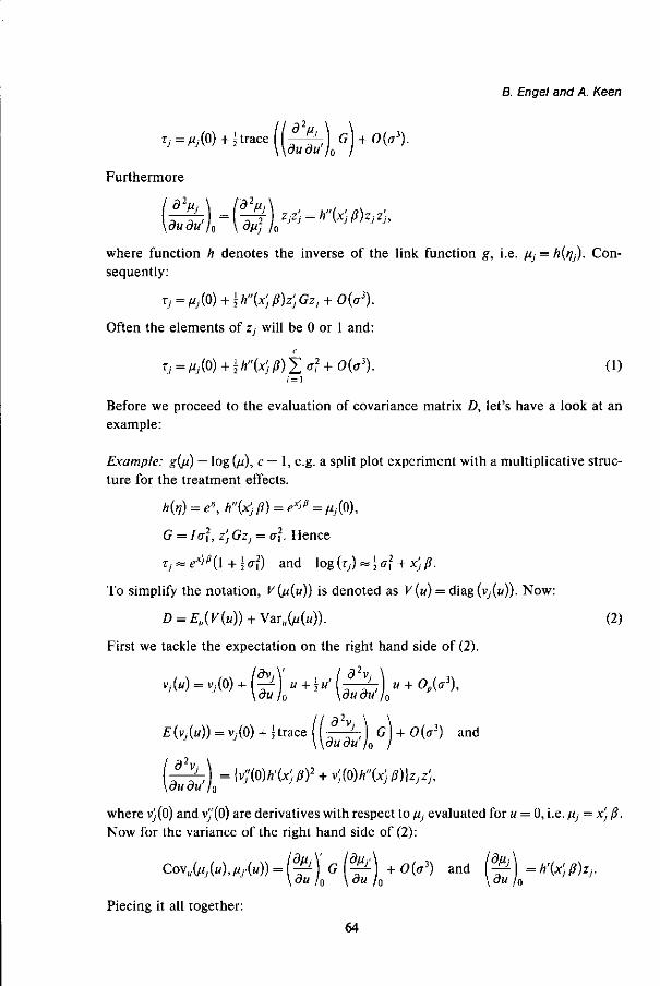
S. Engel and A. Keen
^•^^""((âH^ Furthermore
)2„ \ /"a 2 5 ^ \ /a //, du du' )Adâh'''h'v'p)z'2'-
where function h denotes the inverse of the link function g, i.e. fij = h(rjj). Consequently:
zj = f,j(0) + {h"(x'jß)z'JGzj + O(ai).
Often the elements of z, will be 0 or 1 and:
r ;=/, ;(0)+}/*"(*;/?) X a,2+0((T3). (1) 1 = 1
Before we proceed to the evaluation of covariance matrix D, let's have a look at an example:
Example: g(jj) = log (//), c = 1, e.g. a split plot experiment with a multiplicative structure for the treatment effects.
h(rj) = e\h"{x'jß) = e*'>ß=ßJ(Q),
G = Ia], z'j Gij = a}. Hence
Tj = exJß(\ + \<72) and log (r,) « \ a] + x) ß.
To simplify the notation, V(ji{u)) is denoted as V(u) = diag (v,(w)). Now:
D=Ett(V(u)) + VatMu)). (2)
First we tackle the expectation on the right hand side of (2).
v,.(«) = v;(0) + ( M u + \u' l-f%-\ u + Op{a\ \au /o \dudu /0
£ ( v » ) = v,-(0) + i trace ((J^) <?) + 0(a3) and
9 Vr~) =W;(0)h'(x'Jß)1 + v'i(0)h"(x'jß)}zJz'j, du du' )0
where v)(0) and v"(0) are derivatives with respect to fij evaluated for u = 0, i.e. /Uj = x) ß. Now for the variance of the right hand side of (2):
Piecing it all together:
64

Analysis of generalized linear mixed models
djj = v;(0) + | K(0)A'(x; ß)2 + VjWh'ix} ß) + Ih'ix) /?)2}z; Gz, + 0(a3),
djj. = h'(x'j ß)h'(x'j.ß)z'j Gzy + 0{o\ j +f. (3)
Often, z'j Gzj = 2 / = i a^ while z/ Gz,- is a sum of a subset of a]... a2 representing a covariance on the link scale.
Example (continued): let V(p) =/z, e.g. Poisson data.
h'(x'Jß) = h"(x'Jß) = ex''ß = vJ{0), v;(0) = l, y?(0) = 0. Now
djj « e"Jß + \\ex'iß + 2e2x''ß)a\ and
djy»o\e*>f + *l», j±j',
when^ and yy have one of the random effects in common, 0 otherwise. Hence, ignoring terms of order a\:
dj, ~TJ + <T2T],
djy^alxjTj' or 0, j±j'.
Expressions (1) and (3) may give an impression of the impact of the parameters, the components of variance in particular, on the original scale. The example illustrates that a SS model can motivate the choice of a particular, highly structured, PA model, although the latter model will not always show such agreeable features as in this case. In general, inference and interpretation of results for the estimation procedure proposed in the next section will be mainly restricted to the link-scale. Results on the original scale may be obtained from back-transformation by h(-) = g~'(X correcting, up to first order, for the components of variance.
4 Estimation
The basic algorithm Estimation proceeds in two steps. Step 1 (GLM step):
(i) Conditional upon u, the expectations nhj = 1... N, are estimated by QL; or equi-valently, when the conditional distribution fits within the GLM frame-work, by maximum likelihood. The estimates will satisfy the following equations:
K Ä S ) " - 0 1 -1™«- <4)
P Q
Sißj) = X Xikßk + X ZjmUm, j = 1 ... N, k=\ m=1
where x/k and z/m are elements of vectors x, and z, respectively. Although there
65

S. Engel and A. Keen
may not exist a unique solution for ß k, k = 1... p and « ra, m = 1 ...<?, we will assume that the solution for pj,j = 1 ...N, is unique. The equations may be solved by iterated least squares on a working variate
where fif1 denotes the current value for n} and fif + is obtained from weighted
least squares on ^ ' + 1'. For the final estimates fi/
(J = fr) = (yj-fij)g'(fij) + g(AJ).
For C = (ft... ÇNy, g(fi) = (gfai) - ? W ) ' and V(p) = diag (V(/ij)), to first order:
£ ( C | « ) ~ g M , VarCClKNdiagtgtu) 2 )^) .
Step 2 (LMM step):
(ii) Now the u, will be returned to their proper status as random effects.
E(0 = Eu(E(C\u)^Eu(g(M)) = Xß
Var (C) = £„(Var (CI «)) + Var (£„(C | «)) « £„(diag (g'O/)2) V(ji)) + ZGZ'.
(iii) An estimate is needed, possibly up to an unknown constant o%, of the diagonal matrix
£„(diag (g'iju)2) V(n)) = d W-' = ol diag (w"1).
For the moment suppose that we have acceptable estimates Wj. Later on it will be discussed how these estimates may be obtained. We now have
E(C)*=>Xß, Var(C) « ZGZ' + W~xol,
which is the structure of an ordinary LMM with weights WÏOÏ the residual stratum, (iv) Estimates for the variance components c2, a}... ff2 are obtained by iterated
MINQUE, which is yet another iterated weighted least squares procedure, but now applied to squared and product terms of error contrasts obtained from Ç. Fisher scoring as implemented in Genstat 5, with special features for REML, was used to obtain estimates for the components of variance. The following set of equations will be solved for a2, a\... a2:
ÇPZ, Z'jP( = trace {Z\PZ^, i = 0... c, (5)
with
p = £r' - Qrxx{x'QrlxYlx'Qr\ c
Q = ZGZ' + W~xal = Y oJZ,Z'i + W~X<JI
Estimates for fixed effects ß may be obtained from generalized least squares:
ß = (X'Q-1X)-]X'U-lC, (6)
66

Analysis of generalized linear mixed models
predictions, say û, for random effects may be obtained from regression, similar to best linear unbiased prediction (BLUP) in a LMM:
ü=GZ'U-l(C-Xß), (7)
where Q and G denote Q and G evaluated at the estimates ÓQ ... ô].. Estimates ß and predictions « may be shown to satisfy the mixed model equations:
X'WX X'WZ \jß\ lx' wc
Z'WX Z'WZ + CT0G / \ « / \z'wçj
or in terms of the original observations:
X' Wûiag (gW(y - fi) = X' W{g{ß) - g{fi)) and (9)
Z '^d iag (g'(j2))(y - fi) = Z' W(g(ji) - g{fi)) + a jô" 1«,
where fi is from step 1. Observe that when the link function is the identity, such as is the case in the classical mixed model for normally distributed observations, step (1) simply reproduces the original data: £ = y. In the classical mixed model: V{) = 1 and W = I, step 2 is simply REML on the original observations.
Equations (4), (5) and (6) are the estimating equations for steps 1 and 2 of the estimating procedure. Since REML is based on a normal likelihood for the error contrasts, the estimation procedure shows some similarity to pseudo-likelihood for independent data (CARROLL and RUPPERT, 1988, Ch. 3).
Extending the basic algorithm Step 1 of the algorithm, in some instances, may be rather inefficient. For instance, for an observation with a contribution of a random effect which appears only once in the data, C will be equal to g(y). In such cases step 1 may have to be modified. For example, suppose that offspring of dams are observed, with dam as a random effect, then for offspring of litters with littersize 1, observations should not be analysed conditional upon the dam effect in step 1, i.e. the dam stratum should be pooled with the lowest stratum in the analysis. It is rather tempting to add some extra steps to the estimation procedure, employing the results from step 2, such as:
Step 3a: Update the variable f and weights w and repeat step 2. A prediction of u is needed and an obvious candidate is û from (7). We can go even further;
Step 3b: Repeat step 2, updating Ç and w each time, until convergence. To reduce the computational load, iterated MINQUE may be replaced by ordinary MINQUE, which actually corresponds with one step of the Fisher-scoring algorithm for REML.
With steps 1,2 and 3b, steps 1 and 2 merely serve to generate proper starting values for step 3b. Addition of 3b is intuitively attractive and often computationally feasible. Any
67

B. Engel and A. Keen
theoretical justification of 1,2 and 3b will be asymptotic and will probably also cover the combinations of steps 1,2,3a and of steps 1,2. Whether there is any practical gain in 1,2, 3b or 1, 2, 3a over 1, 2 is not clear yet.
Modification of the basic algorithm for extended variance functions For the extended model, step 2 may have to be modified for the variance function V(ß,(f). The variance function <j> V{fi) offers no special problems since it has no bearing on W. The scale parameter <t> will be equal to, or part of, the residual component a\.
For the more general variance function V(fi, <f) several approaches are suggested in the literature for estimation of <p. WILLIAMS (1982) suggests a method of moments (MM) where 0 is obtained by equating Pearson's chi-square to its degrees of freedom, see also MOORE (1986, 1987) and MOORE and TSIATIS (1991). Another, deviance orientated, approach, is extended quasi-likelihood (EQL) (NELDER and PREGIBON, 1987; MCCULLAGH and NELDER, 1989, §9.6 and Ch. 10.). Pseudo-likelihood (PL) is yet another method which relates both to MM and EQL. For a discussion of PL and EQL see DAVIDIAN and CAROLL (1988) and NELDER and LEE (1991, 1992).
Before we proceed to the estimation of W we will briefly look at a few examples of "extended" variance functions (for convenience dropping indices j referring to the observations):
Examples: (i) V(M,<p)=U + fa\
this is a popular variance function for overdispersed Poisson data (BRESLOW, 1984, 1989, 1990). It is the variance of a negative binomial distribution and may be obtained by sampling the Poisson parameter from a gamma distribution. Ignoring higher order terms, it may also be obtained by adding independent error terms, with mean 0 and variance 0, to the individual observations on the log scale.
(ii) V{ii,4)=M{l-?)(l + 4(n-l)),
this is an example of a variance function for overdispersed binomial data, it is the variance of a beta-binomial distribution (CROWDER, 1978; WILLIAMS, 1982, 1988; PRENTICE, 1986; KÜPPER et al., 1986) and correlated binomial distribution (KÜPPER
and HASEMAN, 1978; ALTHAM, 1978) and relates to the correlated beta-binomial distribution (PAUL, 1987). For a practical example and some discussion see ENGEL
and TE BRAKE (1992). By adding independent errors to the individual probabilities on the logit scale, again with mean 0 and variance <p, ignoring higher order terms, the variance function
"<"•"-" H IHIHI) is obtained.
When the basic algorithm is extended, parameter <p in the extended variance function should be updated as well. For instance, for steps 1, 2 and 3b, by equating Pearson's
68

Analysis of generalized linear mixed models
chi-square to its degrees of freedom, after each repetition of 3b. Note that two of the variance functions discussed in examples (i) and (ii) are approximately in line with the mixed model structure on the link scale, when 0 is positive: the extra variation may be introduced by adding individual error terms on the link scale with variance <p.
Estimation of W We will now turn to the estimation of W. First we will have a look at a number of special, but practically relevant, cases. 1. Log link and quadratic variance function (for quantitative response variables):
g{n) = \og{n), V{li) = ^2. (11)
Now w = 1 and <r2 = <p, i.e all weights are equal. This covers e.g. the analysis of sample variances under a factorial structure.
2. Logit link and "quadratic" variance function (e.g. binomial data):
^)=,ogU-V v^^i^tt. \n-pl n
Again w = 1 and al = <j>. An example is the "leaf-blotch on barley" data, described in MCCULLAGH and NELDER (1989), §9.2.4. In this example percentages of leaf area affected are observed. The data is not binomial, but with ß a percentage, g{/u) = log {nl (100 - n)) and V(p) = ^2((100 - //)/100)2. The variance function may be obtained to first order by introducing a random effect with variance 4> f ° r
logit (u/100) and also follows as the limit for n - oo of Var (lÓOy/n) = ÏOO2 V(ju, <p)/n2, with V(ß,<t>) from (10).
3. When g is the variance stabilizing transformation:
gU2 l
the weights are constant. (1) and (2) are special cases. Other, less important, examples are the square-root transformation in combination with Poisson data and the angular transformation in combination with binomial data. Log link and power variance function:
g(li) = logfa), Vfa) = W,
with a known. Then:
' w~l = Evifo-1) = </>Eu{e(X'^Z'u){a-2)) = <S>ex'^a-1)Eue
z'u cc ^'/»(«-fl
The weights do not depend on the distribution of u. Estimates for quantities (x'i — x'2)ß may be obtained from an ordinary least squares fit on f, ignoring the correlation structure. (1) is a special case. Logit link and binomial variance function:
^ ) = L o g U - ) , K ( , ) = ^ ^ , then
69

s'M = -
B. Engel and A. Keen
1
V(MY
a property defining canonical link functions, and
w =E"[w))= • When the u's are symmetrically distributed:
, £„(ezV)cosh(x7J) + l W cc ,
and for normally distributed w's: Jap
, e y cosh (x'/?) + 1 W cc .
n
For large a,2 relative to ß: w~l oc cosh (x'/?)/n. For small CT,2 relative to ß: w~ ' oc (cosh (x'ß) + l)/n. Often for binary data the of are small, x'ß may be estimated by ordinary least squares on f.
Generally, an obvious estimate for w-1 is w~l = V(fi)g'(fi)2, where fi is obtained from the first step of the estimation procedure. Observe that V(/2)g'{/2)2 may often be an accurate prediction for V(/u)g'(ji)2, but that does not generally imply that it is a consistent estimator for Eu(V(jx)g'(ji)2). To that end the variance components a2 have to be relatively small, otherwise w~l may be an asymptotically unbiased but inconsistent estimator for w_1. When \î>~] = V(/Î)g'(fi)2, it follows from (4) that the lefthand sides of (9) will equal 0 in step 2, or
X'W(g(jl) - g(/;)) = 0 and Z'W{g(fi) - g(ju)) = <r02 G~lu,
the g{fi) are playing the role of observations on the scale of the link function. In many cases it will be possible to improve on w. For the logit link and binomial
variance function in the context of a split plot, for instance, the following procedure may be useful: from estimates for/z (step 1) and Xß (ordinary least squares on Ç after step 1), residuals û may be recovered. An improved estimator, say w, may be obtained by taking bootstrap samples «(,)... W(fl) and evaluating w~x as the mean of V(fi(s))g'(fi(s))
2, s = 1... B, with fi(s) the mean p evaluated in ß and û(sy One advantage of using an improved estimator, more closely approximating Eu{V(ji)g'{ß)2), may be that weights are "smoothed", reducing instability due to the presence of a few extreme weights.
(Asymptotic) properties of the estimators Properties of the estimators should follow from the relevant estimation equations, e.g. (4), (5) and (6) for steps 1,2. For steps 1,2,3b estimation equations follow from (5) and (8) or equivalently (9), replacing fi by ß. Equations (9) simplify to:
70

Analysis of generalized linear mixed models
Z'W diag (g'(ti))(y -p) = ffo2 G'lu.
Clearly these equations are not easy to tackle. The asymptotics of QL (MCCULLAGH,
1983) and (iterated) MINQUE (BROWN, 1976; RAO and KLEFFE, 1988), see also MILLER
(1977), for concistently estimated weights (er,2 -» 0), offer some justification for "large" samples and "small" components of variance. Genstat 5 (1987,1990) produces approximate variances and covariances for estimated fixed effects and components of variance and mean squared errors for the predictions of the random effects for a LMM under normality. These approximations, obtained after step 2 or its last repeat, may be used for the final estimates and predictions in the GLMM. The assumption of normality can be relaxed, but at the least the kurtosis should be close to 0 for the random effects.
Simulation will have to show how well the estimation procedure performs for practical sample sizes. A Monte Carlo study for over-dispersed binomial data is in progress and results will be reported elsewhere.
With an additional non-multiplicative parameter <j> in the conditional variance function, variability due to the estimation of <p is ignored. In some instances this may not be a serious problem, e.g. for V{pi, (f) = / / , 0 is usually restricted to the values 0 = -1,0*, 1,2,3. In other situations, e.g. V(fi,$) =//(l - njn){\ + </>(n - 1)) for "binomial data" where 0 is a correlation coefficient, the ignored variability may seriously affect test results obtained from step 2. Even for independent data the latter problem is still unresolved.
The use of iterated MINQUE, which is equivalent to REML, may be expected to reduce the bias in the estimation of the variance components, relative to maximum likelihood, for normally distributed random effects.
5 Analysis of some data-sets
The preparation of chocolate cakes This is hardly a realistic experiment, but it serves for a comparison with a quasi-likeli-hood based method for (balanced) data with a multiplicative structure for fixed and random effects from FIRTH and HARRIS (1991). The data of this experiment is from COCHRAN and Cox (1957), p. 299. Three recipes for preparing the batter for a chocolate cake were compared. In addition, six different baking temperatures were tested. From a mix made by any recipe, six cakes were baked, one at each temperature. There were 15 replications, replicates representing time differences. The response variable is a "breaking angle", measured for each cake. The 45 batches of cake mix may be considered as "whole plots", with recipes and replicates as whole plot treatment factors. The 6 portions of each batch used to bake the cakes are the "sub plots", with temperature as a sub plot treatment factor. Firth and Harris estimate fixed effects from the quasi-likelihood equations (for non-diagonal covariance matrix of the observations), which for this particular type of model is shown to be equivalent to maximum likelihood based on the gamma distribution. Estimates for variance components are
71

B. Engel and A. Keen
obtained from rather arbitrarily chosen quadratic forms. For non-diagonal covariance matrices the quasi-likelihood Q is defined by a, generally path dependent, line integral. A particular path is chosen and test results are obtained by comparing quasi-deviances — 2Q, referring differences to chi-square distributions, using appropriate scaling factors. For analysis of balanced models with multiplicative effects and errors see also ENGEL, J. (1990) and the next data-set on soldering failures of printed circuit boards.
Y = exßSiE2, E{E) = 1, Var(fi,) = 0,, / = 1,2, £b£2 independent.
Conditional upon whole-plot errors ef.
ß = E{Y\ex) = ex'ߣu
log Cu) = x'ß + log (e,) = (x'ß - £ 00 + «,,
V(fi) = Var(y\ei) = 02S,
where \<j>x is included in the general mean on the log scale, «, is the whole-plot error on that scale: U] = log(e,) + \<j>\ and
£ ( « , ) « 0, Var (Bl) = Var (log (e,)) » Var (e,) = 0,.
In the notation of this paper: o\ = <p\, the variance component for batches, and 0 = <p2, the dispersion parameter of the extended variance function and residual component of variance on the log-scale. As was shown in §4, case ( 1 ), expression ( 11 ): w = 1. Estimates for the components of variance and F-values for the fixed effects R and T x R (R = recipes, T = temperature), are shown in Table 1 for our procedure, for ANOVA on log transformed breaking angles and for the analysis of Firth and Harris, f-values for the main effects of temperature and replicates are < 0.001 in all analyses and omitted from the table.
Table 1. Some results for the chocolate cake data
Type of analysis
GLMM log(angle) and ANOVA Firth and Harris
*? 0.0045 (0.0021) 0.0048 (0.0022) 0.004
02
0.0191 (0.0019) 0.0192 (0.0019) 0.0219
"T*R
0.50 0.52 0.61
PR
0.15 0.16 0.12
GLMM steps 1,2 yield the same results as steps 1,2,3a and steps 1,2,3b. From the table it can also be observed that ANOVA on log transformed breaking angles (assuming in fact the log-normal distribution with whole-plot variance log(l + ^1) and residual variance log (l + 02)) yields virtually the same results as steps 1,2 for the GLMM. This is not surprising for observations with relatively small variation in the means (so that g(y) and its first order approximation £ are close).
Soldering failures in print panels The data is from an experiment with print panels where for each panel the number of soldering failures is observed. The experiment has been carried out with five replica-
72

Analysis of generalized linear mixed models
tions at each combination of three soldering locations and two soldering methods. The thirty panels are the main plots of a split plot design. The sub-plot factor, applied to smaller sub-panels, is the type of copper pattern, at two levels. This data has been analysed by ENGEL, J. (1986, 1990). The data is typically Poisson-type, although extra-Poisson variation may exist. This is the approach taken in ENGEL (1987). In ENGEL
(1990) a multiplicative model, both for fixed and random effects, similar to FIRTH and HARRIS (1991) is assumed. Separate analyses for the error-strata are performed, based on a QL approach with a gamma-type variance function and log link, critically depending on the balance of the design. Estimates for components of variance are obtained by equating Pearson chi-square statistics or quasi-deviances to their expectations. The analysis in ENGEL (1986) is also a combination of separate analyses on the whole- and sub-plot level, employing the Dirichlet multinomial and the negative binomial distribution. At the lowest level, observations are assumed to follow Poisson distributions. Some results for various models and methods for analysis are shown in Table 2, a\ is the whole-plot variance on the log scale, <j> the (over)dispersion parameter for the sub-plots, L x M x P the three factor interaction.
Table 2. Some results for the print panel data
Model/analysis
GLMM Steps 1, 2 (V(/i,t/>) = fo) Steps 1, 2, 3a
Steps 1, 2, 3b
GLMM {V(ii,<p) = <f>fi2)
ANOVA and Log transformation ENGEL (1986)
ENGEL (1990) Approach QA1
6\
0.163 (0.072) 0.189 (0.074) 0.193 (0.077) 0.260 (0.098)
0.248 (0.097)
-0.205 (-) 0.199 (-)
<fi
0.98 (0.28) 0.86 (0.25) 0.90 (0.26)
0.142 (0.041)
0.156(0.045)
Fixed at 1
0.152 (-) 0.142 (-)
'LxUxP
0.09 0.06 0.07 0.01
0.02
0.10
0.01
For the approach referred to as QA1 in ENGEL, J. (1990), the first line corresponds to an estimate (j> derived from a deviance and the second line to an estimate from an appropriate Pearson chi-square statistic. Since the estimator ô\ depends on ij>, there are also two estimates for the whole-plot component of variance. For the GLMM with unequal weights (V(ji,(j>) = 0//), P-values for the three factor interaction are derived by referring the Wald statistic (BUIST and ENGEL, 1991, 1992) to a chi-square distribution. For ANOVA on log transformed data and for the GLMM with variance function <j>ß2, where weights are equal and the balance of the design carries over to the log scale, .F-tests are used. Results for the GLMM with V(ji, <f>) = 0//2 do not change from step 1,2 to step 3a or 3b and also are close to the results of the ANOVA on log transformed data and of QA1. It is easily shown that for balanced data and the variance stabilizing link function the estimate for <j> from step 2 is equal to the traditional estimator obtained from Pearson's chi-square in step 1. Inference with respect to the three-factor-interaction to some extent does depend on the variance function assumed. It is hard to decide which variance function is most appropriate on the basis of the data, although the nature of the
73

B. Engel and A. Keen
problem seems to support the assumption of Poisson variation at the sub-plot level. The estimated dispersion factor is in perfect agreement with this assumption.
Radiation of cancer cells The data set originates from an experiment to measure the mortality of cancer cells under radiation and is presented in SCHALL (1991). Four hundred cells were placed on a dish, and at each of nine occasions three dishes were irradiated. After irradiation the number of surviving cells was counted in each dish. To establish the natural mortality data corresponding to a zero-dose was analyzed. Our results will be compared with Schall's REML type algorithm, see also §6. Considering, apart from the binomial variation at cell level, with a multiplicative dispersion parameter </>, only one component of variance a\ between occasions, at the logistic scale, steps 1 and 2 result in estimates â\ = 0.221 (0.144) and 0 = 1.819 (0.606). Estimates obtained by Schall are almost identical: <T? = 0.225 and <j> = 1.810. Steps 1, 2 and 3b result in estimates â\ = 0.221 and 0 = 1.817, with standard errors as before. <j> > 1 indicates the presence of extra-binomial variation. One way to "explain" the over-dispersion is to introduce an additional component of variance a\ between dishes on the logistic scale. Schall still estimates a multiplicative dispersion parameter 0 and for comparison we do the same, although now it seems natural to fix <p at value 1, i.e. drop </> from the model. With steps 1,2 and 3b, analysing the binary observations per cell, i.e. n = 1, estimates a\ = 0.221, a\ = 0.0098 and $ = 1.002 are found. Schall obtains â\ = 0.222, ô\ = 0.010 and <p = 0.937.
6 Discussion
In an ordinary LMM the random effects can be integrated out of the simultaneous likelihood of observations ƒ and random effects u analytically. Numerical problems mainly involve storage and inversion of large matrices, which to a large extent can be overcome by exploiting the structure of the covariance matrix of the observations, see ENGEL, B. (1990).
In a GLMM with full distributional assumptions, e.g. normality for the random effects u, integration can generally not be performed analytically and maximum likelihood estimation is often bogged down by cumbersome numerical integration routines. Integration is usually by Gauss-Hermite quadrature (ABRAMOWITZ and STEGUN, 1965, p. 924), offering serious problems when a large number of quadrature points is needed and when there are crossed random effects in the model. Little seems to be known about robustness with respect to distributional assumptions for the random effects.
A distinct advantage of the estimation procedure in this paper is that many of the results for LMM's carry over to GLMM's, such as procedures for constructing confidence intervals for components of variance or approximate f-tests for contrasts of fixed effects accounting for variation due to estimation of the components of variance, see ENGEL, B. (1990). The combination of QL and MINQUE, both least squares procedures, offers some scope for robustness. Clearly for a number of practical problems, e.g. relatively small components of variance and fairly large binomial denominators or
74

Analysis of generalized linear mixed models
Poisson means, steps 1 and 2 should produce acceptable results. Extension of the estimation procedure with step 3a or 3b is intuitively attractive and may remove possible inefficiency following from step 1. A formal justification of steps 1,2 and 3b will have to be based on the corresponding estimating equations, which is a tough nut to crack.
Recently, related estimation procedures have been proposed by BRESLOW and CLAYTON (1991) and SCHALL (1991). Schall's REML based algorithm is similar to an extension of our estimation procedure (steps 1, 2 and 3b), except that MINQUE represents a step from Fisher scoring and not from the EM algorithm for REML. The random character of the conditional variances V(/j)g'(fi)2, through their dependence on the random effects u, seems to be completely ignored: the elements of a supposed co-variance matrix in expression (2.3) in Schall's paper are actually random variables. Breslow and Clayton's PQL approach is motivated by quasi-likelihood arguments. The random effects are assumed to be normally distributed, which is equivalent to the use of a sum of extended quasi-likelihoods for identity link and constant variance functions for the sub-vectors ui...uc of«. The quasi-conditional likelihood ofy given u is replaced by a quadratic approximation in terms of the random effects. The quadratic approximation is around the (current) predictions it. The random effects are easily integrated out of the product of the exponentials of the approximate quasi-conditional-likelihood of y given u and the quasi-likelihood of«. This yields an approximate marginal quasi-likelihood for the observationsy. In the derivation, where mathematically convenient, some terms, e.g. g'{n)2V{n), are assumed to vary slowly with p and ignored. Conditional quasi-deviance residuals are replaced by Pearson residuals, which gives a pseudo-likelihood flavour to the method. Not surprisingly the combination of a quadratic approximation and Pearson residuals leads to a normal log likelihood for the IRLS working variable £. A REML type adjustment for loss of degrees of freedom due to estimation of fixed effects, rather poorly motivated in this context, finally yields a REML log likelihood. So, although from quite a different starting point, PQL results in the same algorithm as steps 1,2,3b, possibly except for (minor) differences in the order in which parameter estimates and predictions for the random effects are updated.
Both the quadratic approximation of the quasi-conditional-likelihood and the approximation of quasi-deviance residuals by Pearson residuals in Breslow and Clayton's paper will improve under "small dispersion asymptotics", e.g. large totals « for binomial data or large means for Poisson data. Similar conditions will improve the performance of the MINQUE procedure in steps 2,3a and 3b and the usefulness of the working variable from step 1. The assumption, in the derivation of PQL, that g'(jj)2 V (u) varies only slowly with fi, also requires that components of variance are relatively small.
LONGFORD (1991) develops an approximate maximum likelihood method under full distributional assumptions, e.g. logistic regression with additional normal random effects on the logit scale. He also utilizes a quadratic approximation, but around 0 and not around û, again implying that components of variance should not be too large.
For the data sets we analysed, including the examples in §5, differences with results from specialised methods, e.g. for special link and variance functions or for balanced designs only, were generally small. Present research includes a simulation study of the
75

B. Engel and A. Keen
prope r t i e s of e s t ima t e s f rom s teps 1,2 a nd 1 ,2 ,3a o r 3b , a nd t h e qua l i ty of a pp rox ima t e
va r i ances a nd covar iances a nd W a l d t es t s de r ived f rom t h e last R E M L s tep . A compar i
son w i th m a x i m u m l ike l ihood for no rma l l y d i s t r i bu ted r a n d o m effects a n d a G L M at
t h e lowes t s t r a t um, b o t h w i th r e spec t t o efficiency a nd r obus t ne s s , is a l so cons ide red .
Shou ld t h e e s t ima t i on p r o c edu r e p r e s en t ed in t h i s p ape r ga in in respectabi l i ty , t h e n a
genera l a nd useful t oo l will h ave b e c o m e avai lable to t ackle p r o b l e m s wh i ch so far a re a
s ou rce o f c ons ide rab l e d i scomfor t t o m a n y a n appl ied s ta t is t ic ian.
References
ABRAMOWITZ, M. and I. STEGUN (1965), Handbook of mathematical functions, Dover publications, Inc., New York.
ALTHAM, P. M. E. (1978), Two generalizations of the binomial distribution, Applied Statistics 27, 162-167.
ANDERSON, D. A. A. and J. P. H INDE (1988), Random effects in generalized linear models and the EM algorithm, Communications in Statistics A, Theory and Methods 17, 3847-3856.
BRESLOW, N. (1984), Extra-Poisson variation in log-linear models, Applied Statistics 33, 38-44. BRESLOW, N. (1989), Score tests in overdispersed GLM's, in: Proceedings of GLIM 89 and the Fourth
International Workshop on Statistical Modelling, A. Decarli, B. J. Francis, R. Gilchrist, G. U. H. Seeber (eds.), Lecture notes in statistics 57, 64-74, Springer-Verlag, New York.
BRESLOW, N. (1990), Tests of hypotheses in overdispersed Poisson regression and other quasi-likelihood models, Journal of the American Statistical Association 85, 565-571.
BRESLOW, N. E. and D. G. CLAYTON (1991), Approximate inference in generalized linear mixed models, Technical report No. 106, Department of biostatistics, University of Washington.
BROWN, K. G. (1976), Asymptotic behaviour of MINQUE type estimators of variance components, The Annals of Statistics 4, 746-754.
BUIST, W. and B. ENGEL (1991), A Genstat procedure for testing main effects and interactions in an unbalanced mixed model, Genstat Newsletter 28. In press.
BUIST, W. and B. ENGEL (1992), Procedure VWALD, in: R. W. PAYNE, G. M. ARNOLD and G. W. MORGAN (EDS.), Genstat 5 procedure library, release 2.3, NAG.
CAROLL, R. J. and D. RUPPERT (1988), Transformation and weighting in regression, Chapman and Hall.
COCHRAN, W. G. and G. M. Cox (1957), Experimental designs, 2nd ed., Wiley, New York. CROWDER, M. J. (1978), Beta-binomial Anova for proportions, Applied Statistics 27, 34-37. DAVIDIAN, M. and R. J. CARROLL (1988), A note on extended quasi-likelihood, Journal of the Royal
Statistical Society B 50, 74-82. ENGEL, B. (1990), The analysis of unbalanced linear models with variance components, Statistica
Neerlandica 44, 195-219. ENGEL, B. and J. T E BRAKE (1990), Analysis of embryonic development with a model for under- or
over-dispersion relative to binomial variation, to appear in Biometrics. ENGEL, J. (1987), The analysis of dependent count data, Ph.D. Thesis, Landbouwuniversiteit,
Wageningen. ENGEL, J. (1990), Quasi-likelihood inference in a generalized linear mixed model for balanced
data, Statistica Neerlandica 44, 221-239. FIRTH, D. and I. R. HARRIS (1991), Quasi-likelihood for multiplicative random effects, Biometrika
78, 545-555. Genstat 5 committee (1987), R. W. Payne (Chairman) and P. W. Lane (Secretary), Genstat 5
Reference manual, Clarendon Press, Oxford. Genstat 5 committee (1990), R. W. Payne (Chairman) and P. W. Lane (Secretary), Genstat 5,
Release 2, Reference Manual Supplement, NAG. IM, S. and D. GIANOLA (1988), Mixed models for binomial data with an application to lamb
mortality, Applied Statistics 2, 196-204.
76

Analysis of generalized linear mixed models
JANSEN, J. (1990), On the statistical analysis of ordinal data when extravariation is present, Applied Statistics 39, 75-84.
JANSEN, J. (1992), Statistical analysis of threshold data from experiments with nested errors, Computational Statistics and Data Analysis 13, 319-330.
KÜPPER, L. L. and J. K. HASEMAN (1978), The use of a correlated binomial model for the analysis of certain toxicological experiments, Biometrics 35, 69-76.
KÜPPER, L. L., C. PORTIER, M. D. HOGAN and E. YAMAMOTO (1986), The impact of litter effects on
dose-response modelling in teratology, Biometrics 42, 85-98. LONGFORD, N. T. (1991), Logistic regression with random coefficients, Proceedings of the 6th
International Workshop on Statistical Modelling, Utrecht, 191-202. MCCULLAGH, P. (1983), Quasi-likelihood functions, The Annals of Statistics 11, 59-67. MCCULLAGH, P. (1991), Quasi-likelihood and estimating functions, Ch. 11 of: D. V. Hinkley, N.
Reid and E. J. Snell (eds.), Statistical theory and modelling. In honour of Sir David Cox, FRS., Chapman and Hall.
MCCULLAGH, P. and J. A. NELDER (1989), Generalized linear models, 2nd edition. Chapman and Hall.
MILLER, J. J. (1977), Asymptotic properties of maximum likelihood estimates in the mixed model of the analysis of variance, The Annals of Statistics 5, 746-762.
MOORE, D. F. (1986), Asymptotic properties of moment estimators for overdispersed counts and proportions, Biometrika 73, 583-588.
MOORE, D. F. (1987), Modelling the extraneous variance in the presence of extra-binomial variation, Applied Statistics 36, 8-14.
MOORE, D. F. and A. TSIATIS (1991), Robust estimation of the variance in moment methods for extra-binomial and extra-Poisson variation, Biometrics 47, 383-401.
NELDER, J. A. and R. W. M. WEDDERBURN (1972), Generalized linear models, journal of the Royal Statistical Society A 135, 370-384.
NELDER, J. A. and D. PREGIBON (1987), An extended quasi-likelihood function, Biometrika 74, 211-232.
NELDER, J. A. and Y. LEE (1991), Generalized linear models for the analysis of Taguchi-type experiments, Applied Stochastic Models and Data Analysis 7, 107-120.
NELDER, J. A. and Y. LEE (1992), Likelihood, Quasi-likelihood and Pseudolikelihood: some comparisons, Journal of the Royal Statistical Society B 54, 273-284.
PATTERSON, H. D. and R. THOMPSON (1971), Recovery of inter-block information when block sizes are unequal, Biometrika 58, 545-554.
PAUL, S. R. (1987), On the beta-correlated binomial (BCB) distribution - A three parameter generalization of the binomial distribution, Communications in Statistics A, Theory and methods 16, 1473-1478.
PREISLER, H. K. (1988), Maximum likelihood estimates for binary data with random effects, Biometrical Journal 3, 339-350.
PRENTICE, R. L. (1986), Binary regression using an extended beta-binomial distribution, with discussion of correlation induced by covariate measurement error, Journal of the American Statististical Association 81, 321-327.
RAO, C. R. (1973), Linear statistical inference and its applications, 2nd ed., Wiley, New York. RAO, C. R. and J. KLEFFE (1988), Estimation of variance components and applications, North-
Holland, Amsterdam. SCHALL, R. (1991), Estimation in generalized linear models with random effects, Biometrika 78,
719-728. SEARLE, S. R. (1979), Notes on variance component estimation: A detailed account of maximum
likelihood and kindred methodology, Paper BU-673M. Cornell University, Ithaca, New York. VERDOOREN, L. R. (1980), On estimation of variance components, Statistica Neerlandica 34,
83-106. WEDDERBURN, R. W. M. (1974), Quasi-likelihood functions, generalized linear models and the
Gauss-Newton method, Biometrika 61, 439-447. WILLIAMS, D. A. (1982), Extra Binomial variation in logistic linear models, Applied Statistics 31,
144-148.
77

S. Engel and A. Keen
WILLIAMS, D. A. (1988), Overdispersion in logistic linear models, Third International Workshop on Statistical Modelling, Vienna.
ZEGER, S. L., K. Y. LIANG and P. S. ALBERT (1988), Models for longitudinal data: a generalized estimating approach, Biometrics 44, 1049-1060.
ZEGER, S. L. and M. R. KARIM (1991), Generalized linear models with random effects; a Gibbs sampling approach, Journal of the American Statistical Association 86, 79-86.
Received: February 1992, revised: October 1992.
78

Chapter 5
Analysis of a generalized linear mixed model: a case study and simulation results
Published in: Biomedical Journal (1996) 38, 61-80.
Application of IRREML to a practical problem involving carcass
classification data. The data are fractions. This is a first attempt
to increase confidence in the estimation procedure by looking at
simulation results based on the classification problem.

Biom. J. 38 (1996) 1, 61-80 Akademie Verlag
Analysis of a Generalized Linear Mixed Model: a Case Study and Simulation Results
BAS ENGEL 1 and WILLEM BUIST 2
1 GLW-DLO Agricultural Mathematics Group, Wageningen 2ID-DLO Research Institute for Animal Science and Health, Zeist
Summary
A class of generalized linear mixed models can be obtained by introducing random effects in the linear predictor of a generalized linear model, e. g. a split plot model for binary data or count data. Maximum likelihood estimation, for normally distributed random effects, involves high-dimensional numerical integration, with severe limitations on the number and structure of the additional random effects. An alternative estimation procedure based on an extension of the iterative re-weighted least squares procedure for generalized linear models will be illustrated on a practical data set involving carcass classification of cattle. The data is analysed as overdispersed binomial proportions with fixed and random effects and associated components of variance on the logit scale. Estimates are obtained with standard software for normal data mixed models. Numerical restrictions pertain to the size of matrices to be inverted. This can be dealt with by absorption techniques familiar from e.g. mixed models in animal breeding. The final model fitted to the classification data includes four components of variance and a multiplicative overdispersion factor. Basically the estimation procedure is a combination of iterated least squares procedures and no full distributional assumptions are needed. A simulation study based on the classification data is presented. This includes a study of procedures for constructing confidence intervals and significance tests for fixed effects and components of variance. The simulation results increase confidence in the usefulness of the estimation procedure.
Key words: Components of variance; Mixed model; GLMM; REML; Overdispersion.
1. Introduction
Key properties of the linear model y = \i + e for observations y with means /j, and
v variances a are (i) linear dependence of the mean ft on parameters ßt,...,ß fi = x'ß, with x = (xl...xp)' known and ß = (ß1-..ßp)' unknown, (ii) (functional) independence of the variance a2 of the mean fj. and (iii) mutual independence of observations y. Important extensions of the linear model are the linear mixed model (LMM) (SEARLE, CASELLA and MCCULLOCH, 1992) and the generalized linear model (GLM) (MCCULLAGH and NELDER, 1989).
In a LMM observations may be interdependent, i.e. point (iii) is relaxed. Additional to the residual error terms e, random effects ul...uq are introduced in
81

B. ENGEL, W. BUIST: Generalized Linear Mixed Model
the model: y = x'ß + z'u + e, with z = (z1...z9)' known and u = (u1...uq)' unknown. Observations with elements of u in common are (positively) correlated. An example is the split plot model where the elements of u are the "whole plot errors" and the correlation between observations on the same whole plot is GIKPI + ffe)> where <r„ and a2
e are components of variance "between" and "within" whole plots respectively. In a GLM observations are independent. The mean \i still depends on a linear combination x' ß, now referred to as the linear predictor rj, but through a known link function g: g{n) = r\ = x' ß. The variance may be proportional to a known function of the mean: vax(y) = <f>V(pi). So, (i) and (ii) are relaxed. Well known examples are the logistic regression model for binomial proportions and the log-linear model for Poisson counts.
Sometimes both GLM and LMM features are needed, e.g. a split plot model for proportions. A class of generalized linear mixed models (GLMM) may be obtained by adding random effects to the linear predictor in a GLM structure: r\ = x'ß + z'u, see e.g. ANDERSON and H INDE (1988), PREISLER (1988), IM and GIANOLA (1988) and JANSEN (1990, 1992). The estimation procedure suggested by these authors is maximum likelihood, e.g. for binomial data with normally distributed random effects on the logit scale. To obtain the likelihood, random effects have to be "integrated out". This involves high-dimensional numerical integration, e.g. Gauss-Hermite quadrature (ABRAMOWITZ and STEGUN, 1965, p. 924), with severe limitations on the number and structure of random effects in the linear predictor. Numerical problems with two crossed random effects are insurmountable. In ENGEL and KEEN (1994) an estimation procedure is presented
that does not suffer from these limitations. This procedure is a straightforward extension of the iterative re-weighted least squares (IRLS) algorithm for GLMs (for IRLS see e.g. MCCULLAGH and NELDER, 1989, §2.5), replacing repeated use of weighted least squares on the adjusted dependent variate by repeated use of LMM methodology. This approach is illustrated on carcass classification data. Calculations are performed with standard software for GLMs and LMMs in Genstat 5 (1993). Some aspects of the data are discussed in section 2. The analysis is presented in section 3. Simulation results based on the classification data are presented in section 4. Section 5 includes a brief discussion of the relation to other alternatives for maximum likelihood estimation, i.e. GIANOLA
and FOULLEY (1983), HARVILLE and MEE (1984), GILMOUR, ANDERSON and RAE
(1985), SCHALL (1991), BRESLOW and CLAYTON (1993) and MCGILCHRIST (1994).
2. The Classification Data
In slaughterhouses in the European Community cattle carcasses are visually assessed according to the EC classification system (WALSTRA, 1991). This includes visual assessment of conformation, supported by photographic standards. There are five main classes for conformation: E, U, R, O and P and each main
82

Biom. J. 38(1996) 1
class may be subdivided into three sub classes. Conformation E corresponds to
the convex to superconvex profiles, very rounded with exceptional muscle
development. Conformation P corresponds to the concave to very concave
profiles, with poor muscle development. The data set comprises 575 batches of
carcasses from 23 Dutch slaughterhouses. Batch sizes vary from 25 to 51 with an
average of 46.6. Each batch is independently classified by one of 4 experts and
one of 52 classifiers. The data set is very unbalanced as illustrated by Table 1.
Table 1
Number of batches per classifier and slaughterhouse, illustrating the unbalancedness of the data
Slaughterhouse 1 2 3 4 5 6 7 8 9 10 1112 13 14 15 16 17 18 19 20 2122 23 Total
Class. 1 _ - - — 1 - 6 1 _ - - 1 _. _ _ _ 2 - — - 1 - - 12 2 - 4 - - - 2 - - - - - - - - - 1 - - 2 - - - 1 10 3 _ _ _ _ _ _ _ _ _ _ _ H _ _ _ _ _ . _ _ ! _ _ 15 4 - - - - — — — — — — 1 1 1 - — — — — — — — 1 — 13 5 - — — - 1 - 1 5 — — 1— — — — - 4 - — - — - - 12 6 2 3 - - - 1 - - - 2 - - - 4 - - - 1 - - - - 13 7 - - - - 4 - 4 - - - - - - - 3 - 1 - 1 - - - - - 13 g _ _ _ _ _ _ 4 _ _ _ _ _ _ _ i _ 7 > _ _ _ _ _ _ 12 9 - _ _ - _ - 7 - - - l - - - - - 2 - - - - - - 10
10 - 1 - - - - - - - - - - - - 3 6 - - 3 - - - 1 14 11 - - - - - - - _ 6 3 - - - 2 - - - 3 - - - - - - 14 12 - - - - - - 2 1 - - 1 - - - 2 - 2 - - - - - - 8 13 - - - - - - - - - - - - - - 6 4 - - A - - - - 14 14 _ _ _ - _ _ ! ! _ _ _ _ _ _ _ _ _ _ _ _ _ _ _ 2 15 - - - - - - - - 1 - — - - 2 - — - 1 1 _ - - - - 14 16 - - - - - 1 - - - - - - - 1 5 - 2 - 4 - - - 2 15 17 _ _ _ _ _ _ ! _ _ _ _ _ _ _ ! _ _ _ _ _ _ _ _ 2 18 _ _ _ _ _ _ _ _ _ „ _ _ _ _ _ _ _ _ ! _ _ _ _ 1 19 - - 3 2 - - - - - - - - - - - 1 - - - - - - - 6 20 - 4 _ - - - - - - _ _ - _ 4 - - - - - - - - - 8 21 - - - - - - - - - 1 2 - - - 5 - - - 3 2 - - - - 13 22 _ _ _ _ _ _ _ _ _ _ _ _ ! _ _ _ _ _ - _ _ _ i 23 _ _ 9 3 - - - - - - - - - - - 3 - - - - - - - 15 24 _. - 2 - - - - - - - - - - 1 - - - - - - - - _ 3 25 - - - - 1 - 2 4 - - - 1 - - - - 7 - - - - - - 15 26 - _ 6 3 - - - - - - - - - 1 - 1 - - - - - - - 11 27 - - - - - - - - - - _ _ _ ! _ _ _ _ _ _ _ _ _ i 28 - 1 - - - - - - - - - - - - - 8 - - 6 - - - 1 16 29 - 2 - - - 2 - - - - - - - - - 2 - - 4 - - - 3 13 30 1 - _ - - - _ _ _ 4 - - - 3 _ _ _ - _ 4 _ _ _ 12 31 _ _ _ _ . - _ _ _ _ _ 2 9 - - - - - - - - l - 12 32 - - - - - - _ _ _ _ _ 2 12 - - - - - - - 1 - - 15 33 - - - - - - 5 - - - - 1 _ _ _ _ 5 _ _ _ l _ _ 12 34 - - - 3 - 4 - - - - 1 - i - _ - - - _ - _ _ 9
83

B. ENGEL, W. BUIST: Generalized Linear Mixed Model
Table 1
Class.
35
36
37
38
39
40
41
42
43
44
45
46
47
48
49
50
51
52
Total
(continued)
1
-
-
2
1
-
2
-
2
-
-
_
5
1
3 4 5
- - 2 - - -
- - 1
-_ _ _
_ _ _
-_ - _
_ _ _
8 21 20 8 13
6
-
-
-
_
1
_
-
7
1
3
3 -
1
7
_
-
1
1
10
5
8
9
2
2 -
3
_
-
2
-
9
_
-
1
1
-
1
-
1 --
-
Slaughterhouse
10
_
-
4
2
3
-
_
-
1
-
1
7 69 30 12 22
11
1
2
_
-
-
-
1
1
-
9
12
_
-
-
1
1
-
_
-
1
_
-
13
_
-
-
10
_
-
_
-
2
7
14 15
—
-
4
1
1
6
3
3
1 -
5
9
_
-
-
_
-
—
-
3
-
16
—
-
-
_
-
_
-
_
1
17
2
3
4
3
_
-
3
2
7
10
18
_
-
4
_
-
4
-
1
7
19 20 21 22 23
-
-
-
_
-
_
2
7
8
12 65 59 24 27 66 34 44
_ _
_ _
1 -
_ _
- -
_ _
- -
_
- -
5 4
-
-
2
_
-
_
-
_
-
4
_
-
-
-._
_
-
_
4
_
-
12
Total
13
6
12
14
14
3
6
12
14
4
8
1
12
5
3
43
1
48
575
Proportions of equal scores per batch are analysed, introducing classifiers as random effects. Interest lies in variation between classifiers, i.e. in components of variance associated with main effects and interactions for classifiers. The "raw" mean of the fractions of agreement over all the batches is 0.63. The means for the experts are 0.60, 0.61, 0.63 and 0.65. Means for the slaugterhouses vary from 0.52 to 0.77.
3. Analysis of the Classification Data
3.1 Getting started
Estimation starts with a logistic regression model (Cox and SNELL, 1990), including classifier effects as fixed effects. Observation yt for batch t,t=l...N,is the fraction of carcasses with an equal score from expert and classifier. Expectation nt of y, is the probability of agreement between expert and classifier for a typical carcass at the particular slaughterhouse. The linear predictor r\t = log(Ju,/(l — n,)) is a combination of main effects and interactions for slaughterhouses, experts and classifiers. Visual assessment of conformation is influenced by many factors, most of which are not very well known. Over-dispersion is quite likely and the variance of an observation is assumed to be:
84

Biom. J. 38 (1996) 1
var(y() = 4>/i,(l-/!()/nr, (1)
where </> is an unknown dispersion factor and nt is the batch size. Parameters are estimated by maximum quasi-likelihood (QL) (MCCULLAGH
and NELDER, 1989, Ch.9) with the IRLS algorithm, using standard software in Genstat 5. Quasi-deviances for various models fitted to the data are presented in Table 2. Tests for interactions are derived by scaling the difference between the déviances of two nested models by an estimate $ for the dispersion factor, referring the result to a chi-square distribution. Estimate $ is equal to Pearson's chi-square statistic divided by its degrees of freedom (MCCULLAGH and NELDER,
1989, §4.5. and Ch. 9), evaluated for the largest of the two models. Model 5, with main effects and interactions between experts and slaughterhouses and between experts and classifiers, describes the data adequately and will be used in subsequent steps of the estimation procedure. In this model $=1.29 (0.094), where the standard error (in parentheses) is based on approximation by a chi-square distribution with 375 degrees of freedom. The same approximation shows that 4> is significantly larger than 1.
Table 2
Quasi-deviance and Pearson's chi-square statistic for various models fitted to the classification data. C, S and E denote main effects for classifiers, slaughterhouses and experts respectively, C.S denotes interaction between classifiers and slaughterhouses etc.
Model Quasi- Degrees of Pearson's deviance freedom chi-square
1 C + S + E + C.S + C.E + S.E + C.S.E 2 C + S + E + C.S + C.E + S.E 3 C + S + E + C.S + C.E 4 C + S + E + C.S +S.E 5 C + S + E +C.E + S.E 6 C + S + E 7 C + S + E +C.E 8 C + S + E +S.E
For use in subsequent steps of the estimation procedure note that the adjusted dependent variate (, of the IRLS algorithm, corresponding to the fitted values fit, is:
Ct = (y,-ß,)g'(ß,) + g(fi,)-
Approximate mean and variance are:
£(C,)*g(ju,) and var(Ct)^g'(fit)2\ar(y,), (2)
as follows from (ju, — fit) g'(/2,)«g(^,) — g(/î,), where g' is the derivative of the link function with respect to /x,.
85
375.0 377.8 429.9 470.5 490.4 725.9 562.3 643.1
284 288 309 339 375 498 409 454
369.1 372.0 423.5 461.9 482.9 712.5 553.6 631.1

B. ENGEL, W. BUIST: Generalized Linear Mixed Model
3.2 Fitting a LMM to the adjusted dependent variate
Classifier effects will now be introduced as random effects on the logit scale. Let X and Z = (Zj,Z2) be the design matrices for the vectors ß and u = (u1',u2')' of fixed and random effects, respectively. Elements of u are uncorrelated with zero means and variances a\ for the classifier main effects in vector Ht and a\ for classifier * expert interactions in vector u2. Without loss of generality X is assumed to be of full rank. The total variance on the logit scale is a1 = a\ + o\ and the correlation between any two random contributions for the same classifier but different experts is Q = ó\j{a\ + a\). For a formal derivation of the model see section 5. The vector of linear predictors r\ = logit (/i) = X ß + Zu, where fi = E(y\u) is the vector of conditional means and y the vector of observations. Conditional variances are \&r(yt\u) = 4>nt{\ — nt)/nt = 4> V{ßt), say.
The mean and variance presented in (2) are conditional upon the random effects. The marginal mean and covariance matrix are approximately:
E(C)xXß and v a r ^ ^ Z / a ? + Z2Z2'a\ + </> W~l,
where W is a diagonal matrix with diagonal elements wt = (g'(fit)2 V(fit))~
l. This is a LMM structure for £ with weights wt on the "residual" error stratum and dispersion factor (j) in the role of a residual error variance. For details see ENGEL
and KEEN (1994). Components of variance and dispersion factor <}> are estimated by Iterated
Minimum Norm Quadratic Unbiased Estimation (I-MINQUE).
Dependence of MINQUE (RAO, 1973, §4j) on a priori values disappears when it is iterated, using successive estimates as a priori values, yielding 1-MINQUE with more attractive (asymptotic) properties (BROWN, 1976). I-MINQUE is essentially an iterated weighted least squares method, see SEARLE et al. (1992, Ch. 12), and there is no need for full distributional assumptions. Ignoring non-negativity constraints, estimating equations for restricted maximum likelihood (REML) (PATTERSON and THOMPSON, 1971) and I-MINQUE are the same (see e.g. SEARLE et al., 1992, p. 397-399), i.e. the two methods are operationally equivalent. We used the REML facilities of Genstat 5.
Estimating equations for the components of variance are:
C'PZm^mZ„1'PC = t race(Zm 'PZm^J, m = 0 , l ,2 , (3)
where P = ß _ 1 - f l _ 1 A' (A ' ' ß _ 1 A' )~ 1 A"ß _ 1 , Q = ZlZi,a\ + Z2Z2a
22 + 4> W~\
A0 = W~1 and Z0, Al,A2 are identity matrices. Solutions are: a\ = 0.0144 (0.0081), d\ = 0.0062 (0.0083) and #=1.379 (0.096) for the components for classifier main effects, classifier * expert interaction and residual (dispersion factor), respectively. Standard errors (in parentheses) are obtained with Genstat and based on Fisher information under normality for an ordinary LMM, see section 5.
Estimates ß for the fixed effects and predictions û for the random effects may be obtained from the following mixed model equations (MMEs) (see e.g. SEARLE
etal., 1992, §7.6.):
86

Biom. J. 38 (1996) 1
'x'wx x'wz \ (ß\_(x'&£\ \Z'WX Z'WZ + (f>Gx) \u)~\Z'tVCj' ( )
Here Q and G = Var(u) are evaluated for the estimates à\, à\ and $.
In a LMM ß is the generalized least squares estimator, û is referred to as the best linear unbiased predictor (BLUP) (see e.g. ROBINSON, 1991). The MMEs can be reduced in size by elimination of main effects and interactions corresponding to a factor with many levels, typically the classifier main effects and expert * classifier interactions in the classification data. In animal breeding theory this process is referred to as absorption (see e.g. ENGEL, 1990). Genstat allows to define an absorbing factor, interactions with the absorbing factor are automatically absorbed as well. Equations (3) may be formed from bits and pieces of the MMEs (4) and their solution (/?', û')'.
Here the estimation procedure might stop. However, it is quite tempting to update the adjusted dependent variate and weights, employing the estimates ß and predictions û from (4), and repeat the LMM step until convergence. We will do so in the next section.
3.3 Iterating on
One step of MINQUE suffices in each repeat of the LMM step. MINQUE is equivalent to one step of the Fisher scoring algorithm for REML (SEARLE et al., 1992, p. 397-399). Genstat uses Fisher scoring and we simply restricted the algorithm to perform one step only. Final estimates are a\ = 0.0137 (0.0082), a\ = 0.0092 (0.0088) and <f> = 1.364 (0.095), for classifier main effects, classifier * expert interaction and residual respectively. These estimates are very similar to those obtained in the previous section, as judged by their standard errors. The total variance â2 = è\ + a\ = 0.0229 (0.0084) and the correlation Q = ô2/(âj + <T ) = 0.60 (0.33).
With the Wald test (BUIST and ENGEL, 1992), after approximation with a chi-square distribution with 44 degrees of freedom, the interaction between experts and slaughterhouses is close to significance (P = 0.06). Estimated means on the logit scale for the 70 combinations of experts and slaughterhouses vary from -0.2291 (0.3564) to 1.2204 (0.4069). One way to proceed is to choose a number of typical values for the linear predictor and describe the variation between classifiers around those levels.
Suppose that r\ is one of the typical values for a combination of expert and slaughterhouse. For a random classifier an approximate 0.95 prediction interval for the linear predictor is: t\±_ 1.96 â, say (r\-\r)+). The corresponding 0.95 prediction interval for the probability of agreement is: (1/(1 +exp( — rj_))\ 1/(1 +exp( — »/ + )). For small a2 the average probability of agreement is approximately: 1/(1 + exp( — rj)), say p(r\), and the range of the interval is: 3.92 op(rj) (1 — p(//)).
Another approach, followed here, is to assume that slaughterhouse and expert * slaughterhouse effects are random as well, with the following results: d\ = 0.0143 (0.0074), af = 0.0071 (0.0076), 6\ = 0.0092 (0.0078), a\ = 0.0109 (0.0077) and $ = 1.379 (0.094) for the classifier main effects, expert * classifier interaction,
87

B. ENGEL, W. BUIST : Generalized Linear Mixed Model
slaughterhouses main effects, expert * slaughterhouse interaction and residual, respectively. The Wald test for experts is not significant (P = 0.14), indicating that differences between experts are relatively small. The mean levels for the 4 experts on the logit scale are: 0.3942 (0.0625), 0.4432 (0.0692), 0.5295 (0.0488) and 0.5473 (0.0609). The average standard error of a difference between two experts is 0.0769. The overall level is 0.4786 (0.0382). The total variance due to classifiers is (T2 = 0.0214 (0.0078) and correlation ^ = 0.67 (0.31). For jj = 0.4786, the approximate 0.95 prediction interval for the probability of agreement is: (0.548; 0.683). Intervals of similar width are obtained for the separate experts. Hence, the range of the probability of agreement between classifier and expert is about 0.135 (0.024), due to differences between classifiers, around an average level of about 0.62 (0.02). The size of the range indicates that there is still scope for improvement.
Scaled residuals for Ç are equivalent to Pearson residuals for the original fractions of agreement evaluated for ß and û from (4). Plots of these residuals do not indicate that the assumed variance (1) is inadequate. A normal probability plot of the residuals does not indicate any serious departures from normality for the random effects, which gives some reassurance for the use of the approximate variances and covariances (see section 5).
4. A Monte Carlo Study
Simulation is based on the classification data. To reduce the amount of calculation involved, the model is restricted to main effects only. Furthermore, conditional upon the classifiers, data are generated from binomial distributions. Consequently the dispersion factor <\> is identical to 1, although it is assumed to be unknown in the estimation process. Random classifier effects are generated from a N (0, a\) disribution. Several parameter configurations are studied. For each configuration 1000 simuations are performed. a\ and <j) are updated until the absolute change in successive iterates is less than 0.0001 times the value of the last update but one. When this does not occur within 25 iterations, estimates from the 25th iteration are considered to be the final estimates. A negative value for a\ is replaced by 0.0001 of the estimate for (p.
Note that in some problems it could make sense to allow the estimates to remain negative, as long as the covariance matrix on the link scale remains positive definite, thereby allowing for negative correlation on the link scale as well (e.g. SEARLE et al., 1992, §11.2).
To see how some of the methods available for ordinary mixed models perform for a GLMM when applied to the adjusted dependent variate, the Wald test for fixed effects, two procedures for constructing a confidence interval for the ratio y = a\/(j) (SEELY and EL-BASSIOUNI, 1983; HAR VILLE and FENECH,
1985) and for the "residual variance" </>, and an F-test for the hypothesis o\ = 0, are studied.

Biom. J. 38 (1996) 1
In "ordinary" over-dispersion models, see e.g. BRESLOW (1990), WILLIAMS (1991), the Wald test, quasi-score test and quasi-likelihood ratio test are proposed for testing parameters in the linear predictor. Without full distributional assumptions the latter two tests have no obvious direct extension to the GLMM model. In BRESLOW and CLAYTON (1993) an approximate quasi-likelihood for a GLMM is derived, which motivates the estimating equations for the components of variance. However, it is not clear whether this leads to a suitable test criterion. The Wald test easily extends to GLMMs. It performs well in a limited simulation study by WILLIAMS (1991) for over-dispersion models and is easily calculated from the approximate variances and covariances produced by Genstat. Therefore this test was chosen for a first impression of test results for fixed effects in a GLMM model.
In a LMM under normaliy the confidence intervals and the F-test are exact. In a GLMM they are approximate. In the simulation, to evaluate the coverage probability of the interval for y, we only need to check whether the true y is in the interval or not. To this end it is sufficient to check whether the pivotal quantity Q(y) = {(£' Wê - RSS)/51}/{RSS/498} is in between the 2.5 and 97.5 percentage points of the F-distribution with degrees of freedom 51 (for classifiers) and 498 (for residual). RSS is the residual sum of squares in an ordinary analysis of variance on £ with all effects, including classifiers, entered as fixed effects and with weights w,. Weights w, are evaluated for y, and residuals ê = f — X 9 — Zû for the true y. For the actual construction of the interval, which is most easily done by plotting Q against y, an expression from HARVILLE and FENECH (1985) in terms of eigenvectors and eigenvalues is appropriate. These eigenvectors and eigenvalues have to be calculated only once and apply to all values y considered. The confidence interval for <j> is derived from RSS employing a chi-square distribution with 498 degrees of freedom. The approximate F-test for the hypothesis a\ = 0, which is closely connected with the pivotal quantity Q, is the F-test for classifiers in the model with fixed classifier effects and residual sum of squares RSS.
4.1 Configurations of parameter values
The following factors are varied in the simulation: The number of batches: Nt: number N = 288, "half" of the original design; N2: number N = 575, same design as for the actual data.
The design under N2 for the batches is the same with respect to slaughterhouses, experts and classifiers as for the original data. To obtain "half" of this design, for N t half of the batches were randomly selected from the original design. This new design was used in all simulations involving 288 batches. Due to the random selection of batches, for Ni there is one slaughterhouse less than for N2. Batch sizes were varied under N1 and N2, as shown below, by dividing the original batch sizes by 1, 2, 3, 5 or 10 and rounding to the nearest integer below. - The batch sizes:
Bi: batch sizes n/10 (n= 4.6); B2: batch sizes nj 5 (n= 9.3); ß3 : batch sizes nj 3 (n = 15.0); ß4 : batch sizes nj 2 (n = 23.3); ß5 : batch sizes n from the actual data (n = 46.6).
89

B. ENGEL, W. BUIST : Generalized Linear Mixed Model
Average batch sizes refer to N2. For N t the average batch sizes for Bt to B5 are 4.7, 9.5, 15.2, 23.7 and 47.5, respectively.
- The component of variance for classifiers: Ci:«r? = 0; C2: o-j =0.02 (same order as for the actual data); C3:<r? = 0.2.
The fixed effects for experts: Fx: 0, 0, 0,0; F2: -0 .11 , -0.05, 0, 0.01 (similar to the actual data); F3: -0.22, -0.10, 0, 0.02; F4: -0 .33, -0.15, 0, 0.03.
The contrast between experts 1 and 4, with values 0, —0.12, —0.24 and —0.36 for Fv F2, F3 and F4 respectively, will be referred to as cE. Estimates and estimated standard errors of this contrast are inspected in the simulation. Slaughterhouse effects are regarded as nuisance parameters, their values are taken from the analysis of the actual data. Pairwise differences between slaughterhouses on the logit scale gradually vary from about 0 to 1.
Configurations are coded with respect to the factors N, B, C and F and for ease of reference also consecutively numbered in Tables 4, 5 and 6.
4.2 Convergence
The number of iterations, i.e. repeats of the LMM step, needed to satisfy the convergence criterion, is in most cases less than 10. Worst cases are configurations with classifier component a\ = 0 or batch size around 5.
For these configurations the percentage of simulations where the number of iterations exceeds 10 may run to about 15%, with about 3% needing 25 or more interations. For <r?=0, the estimation procedure is slowed down because the optimum is close to or on the boundary; some 60% of the simulations produce a negative estimate for a\. For small batch sizes, there is little information in the data about a\ and about 25% of the simulations may produce a negative estimate for the classifier component.
4.3 Results for bias
Table 3 shows estimated bias terms for component a\, dispersion parameter <p and contrast cE as a percentage of the true value. Also shown are the standard error of the bias percentage (in parentheses) and 0.05 and 0.95 quantiles (between square brackets) of the estimated parameter values, derived from the 1000 simulations.
90

Biom. J. 38 (1996) 1
Table 3 Bias of a\, (f> and cE presented as a percentage of the true value, except when the true value is 0 (underlined). The corresponding standard error is in parentheses. 0.05 and 0.95 quantiles of the estimated values for <s\, (j> and cE from the 1000 simulations are between square brackets. The last column shows the percentage of negative estimates for a\.
Conf. a\ <j> cE % nr. N B C F %bias (s.e.) [quantiles] %bias (s.e.) [quantiles] %bias (s.e.) [quantiles] comp.
neg.
10 11 12 13 14 15 16
20 21 22 23 24 25 26
27 28 29 30 31 32 33
-0.1 0.0 0.0
-0.1 0.7 0.8 0.9 0.9
(0.69) (0.69) (0.69) (0.68) (1.02) (1.03) (1.03) (1.03)
[0.13 [0.13 [0.13 [0.13 [0.01 [0.01 [0.01 [0.01
0.0006 (0.0000) [0.000:
-1.1 -1.0 -0.9 0.2 0.7 1.1
(0.72) (0.72) (0.72) (1.32) (1.31) (1.32)
[0.13 [0.13 [0.13 [0.01 [0.01 [0.01
0.0014 (0.0001) [0.000
17 2 3 3 2 18 2 3 2 2 19 2 3 1 2
-0.6 (0.78) -1.4 (1.63) 0.0019 (0.0001)
1 1
[0.12 [0.00 [0.000:
[0.12 [0.13 [0.12 [0.00 [0.00 [0.00
0.0033 (0.0002) [0.000
-0.6 -0.4 -0.4 4.5 5.4 5.5
(0.84) (0.84) (0.84) (2.16) (2.16) (2.17)
0.2 0.5 0.4
14.6 13.5 13.3
(1.04) (1.04) (1.04) (3.27) (3.30) (3.33)
[0.10 [0.10 [0.10 [0.00 [0.00 [0.00
0.0071 (0.0004) [0.000
0.28 0.28 0.28 0.28 0.03 0.03 0.03 0.03 0.033
0.28 0.28 0.28 0.03 0.03 0.03 0.006
0.28 0.04 0.009;
0.29 0.28 0.30 0.05 0.05 0.05 0.015
0.32 0.32 0.32 0.06 0.06 0.06 0.031
1.1 (0.20) 1.1 (0.20) 1.3 (0.20) 1.3 (0.20) 0.6 (0.20) 0.5 (0.20) 0.5 (0.20) 0.4 (0.20) 0.3 (0.20)
[0.91 [0.91 [0.91 [0.91 [0.90: [0.90: [0.90: [0.90; [0.90
1.0 (0.21) [0.91 1.0 (0.21) [0.90: 1.0 (0.21) [0.91 0.3 (0.19) [0.90: 0.2 (0.19) [0.90: 0.2 (0.20) [0.90; 0.2 (0.19) [0.90;
1.2 (0.20) [0.91 0.6 (0.19) [0.91 0.4 (0.19) [0.91
0.6 (0.19) [0.91 0.7 (0.19) [0.91 0.7 (0.19) [0.92 0.2 (0.19) [0.91 0.2 (0.19) [0.91 0.2 (0.19) [0.91 0.2 (0.19) [0.91
0.4 (0.17) [0.92 0.3 (0.17) [0.92 0.3 (0.17) [0.92 0.6 (0.17) [0.92 0.4 (0.17) [0.91 0.4 (0.17) [0.91 0.6 (0.17) [0.92
1.11] 1.12] 1.12] 1.12] 1.12] 1.12] 1.12] 1.11] 1.11]
1.12] 1.12] 1.12] 1.11] 1.11] 1.11] 1.10]
1.12] 1.11] 1.10]
1.11] 1.12] 1.11] 1.11] 1.10] 1.10] 1.10]
1.09] 1.09] 1.09] 1.09] 1.09] 1.09] 1.10]
0.47 0.71 1.3 0.0007 0.06 0.25 0.67 0.0011
-0.33
0.92 2.5 0.0019 0.39 1.4 0.0012 1.6
0.42 -1.1 -1.4
1.6 4.1 0.0036 0.44 1.2 0.0028 0.77
2.2 6.4 0.0068 0.25 2.8 0.0060 2.8
8.4 0.0101 2.7 8.8 0.0109 9.4 0.0116
-1.8
2.5
10.3 0.0149
13.8 0.0209
13.8 0.0215
(0.41) (0.61) (1.23) (0.047) (0.38) (0.58) (1.17) (0.045) (
(1.15)
(0.61) (1.84) (0.002) (0.58) 1.78)
(0.069) (1.72)
(2.20) 2.12)
(2.06)
(0.91) (2.80) (0.003) (0.87) (2.67) (0.003)
(2.58)
(1.29) (3.88) (0.005) (1.24) (3.79) (0.005) (3.72)
(2.77)
(0.003) (0.88) (2.63) 0.003) 2.54) [ 0.003) [
3.09) [
4.24) [
5.98) [ 0.007) f 6.03) [ 0.007) f 6.01) [ 0.007) 1
;-0.43; -0.31; -0.20;
;-0.08; ;-0.43; 1—0.31; ;-0.19; ;-0.07;
;-o.i9,
-0.47; -0.22;
1—0.11; ;-0.46; ;-0.22; I—0.11; ;-0.22;
-0.26; ;-0.25; ;-0.25;
-0.53; -0.29;
;-0.17; -0.52;
;-0.28; ;-0.16; ;-0.28;
-0.59; -0.36;
;-0.23; -0.60;
;-0.36; -0.25;
;-0.36;
;-0.28; -0.17;
-0.51; i-0.27; -0.15; -0.27; -0.15;
-0.31;
-0.39;
-0.50; -0.36; -0.49; -0.37; -0.48; -0.34;
-0.28] -0.16] -0.04] 0.08]
-0.29] -0.17] -0.04] 0.07]
-0.24] 0.00] 0.12]
-0.25] 0.00] 0.11]
-0.05] 66
-0.01] 61
0.02] 0 0.01] 3 0.01] 66
-0.19] 0 -0.06] 0 0.18] 0
-0.19] 8 0.05] 8 0.17] 8 0.04] 63
-0.10] 0 0.14] 0 0.25] 0
-0.12] 23 0.13] 25 0.24] 25 0.11] 59
34 35 36 37 38 39 40
41
42
43 44 45 46 47 48
-0.9 -0.9
2.3 3.1 3.3
1 1
(0.85) (0.85) (1.96) (1.95) (1.96)
0.0027 (0.0001) [0.000: 0.0027 (0.0001) [0.000:
[0.12 [0.12 [0.00 [0.00 [0.00
1 3 2 2
1 2 2 2
1 1 1 1 1 1 1 1
3 2 3 1 2 2 2 1
1 1 1 2 1 1 1 1
(2.46) [0.00
(3.54) [0.00
(1.43) [0.07 (1.45) [0.06 (5.42) [0.00 (5.31) [0.00
0.0136 (0.0007) ro.00 0.0135 (0.0007) [0.00
1.1
16.6
1.2 1.2
49.3 47.9
0.30 0.30 0.04 0.04 0.04 0.012 0.012
0.05
0.07
0.36 0.37 0.10 0.10 0.06 0.06
1.3 (0.30) [0.87 1.4 (0.30) [0.86 0.5 (0.29) [0.86 0.4 (0.29) [0.86 0.4 (0.29) [0.86 0.3 (0.29) [0.86: 0.3 (0.29) [0.86:
0.3 (0.29) [0.86:
0.7 (0.30) [0.87
0.7 (0.26) [0.88 0.7 (0.26) [0.87 1.2 (0.27) [0.88 1.2 (0.27) [0.88 1.3 (0.27) [0.87 1.3 (0.26) [0.88
1.17] 1.17] 1.16] 1.16] 1.16] 1.15] 1.15]
1.15]
1.18]
1.15] 1.15] 1.16] 1.16] 1.16] 1.15]
0.06] 0.19]
-0.18] 0.06] 0.19] 0.05] 66 0.18] 64
0.07] 15
0.14] 28
0.26] 1 0.41] 0 0.27] 39 0.42] 37 0.28] 62 0.40] 61
91

B. ENGEL, W. BUIST: Generalized Linear Mixed Model
Results for JV2 (575 batches) are shown in the top half of the table. Only for small batch sizes and small component a\ for classifiers, the percentage bias in a\ is sizeable, in all other cases the bias is negligible. The larger bias percentages go together with high probabilities for a negative estimate for the classifier component, as shown in the last column of the table. For instance in configuration 31 the estimated probability for a negative estimate is 0.25. But even for this configuration, where the estimated percentage bias is 13.5%, the estimates are hardly misleading since the corresponding standard errors (see Table 4 discussed below) are of the same order as the estimates, reflecting the fact that the data convey little information about the component. Although the bias for cE runs to 6.4% for configuration 28, none of the estimated bias terms is significantly different from zero.
For Nt (288 batches) for small batch size and small classifier component, large bias in a\ is found. For configuration 45 the classifier component is overestimated by a factor of almost 1.5. The estimated probability for a negative estimate for o\ is 0.39 for this configuration. For larger batch sizes, e.g. in configuration 37, bias is small. Bias for cE is appreciable and runs to some 14% for the smaller batch sizes. However, this is the same order of bias as for ordinary logistic regression for data configurations such as these. Configuration 39 for instance, shows an estimated bias percentage of 9.4 (2.54) %, while ordinary logistic regression on the same data, ignoring classifiers, yields a similar estimated bias of 9.8 (2.54)%.
Although the bias in <j>, for some configurations, is significantly different from 0, it is negligible in all cases studied. An alternative estimator for </> is SSR divided by the appropriate number of degrees of freedom for iVx and N2. Results for this estimator are similar to those reported in Table 3.
4.4 Results for standard errors of estimates
Table 4 shows the standard errors of the estimates as derived from the 1000 simulations. These standard errors are referred to as the "empirical" standard errors. Also shown are the mean and 0.05 and 0.95 quantiles of the standard errors produced by Genstat in the 1000 simulations.
Observe that for N2 the mean standard error for cf> produced by Genstat is similar to the value j/(2/498) = 0.0634 based on a chi-square distribution with 498 degrees of freedom. For decreasing batch sizes, the standard error tends to be over-estimated. For small batch sizes the chi-square approximation becomes less appropriate (asymptotics are with respect to n—• oo); the true distribution is somewhat shorter tailed. However, the estimated 0.05 and 0.95 quantiles in Table 3 are about 0.92 and 1.09 and quite similar to the values 0.90 and 1.11 for the #498/498 distribution, as derived with the Wilson-Hilferty approximation (ABRAMOWITZ and STEGUN, 1965, 26.4.14, p. 941). For Nt
the standard error based on a chi-square distribution with 212 degrees of freedom is 0.0971 and the quantiles are 0.85 and 1.16. It seems that a size 0.05 test for over- or underdispersion, employing a chi-square approximation, would not do too badly; it tends to be somewhat conservative.
92

Biom. J. 38 (1996) 1
Table 4 Standard errors of estimates. The "true" (empirical) standard error from the 1000 simulations and the mean and 0.05 and 0.95 quantiles of the estimated standard errors produced by Genstat.
Conf. nr.
1 2 3 4 5 6 7 8 9
10 11 12 13 14 15 16
17 18 19
20 21 22 23 24 25 26
27 28 29 30 31 32 33
34 35 36 37 38 39 40 41 42
43 44 45 46 47 48
°î N B C F emp. mean [quantiles]
2 5 2 5 2 5 2 5 2 5 2 5 2 5 2 5 2 5
2 5 2 4 2 4 2 4 2 4 2 4 2 4
2 3 2 3 2 3
2 2 2 2 2 2 2 2 2 2 2 2 2 2 2 1 2 1 2 1 2 1 2 1 2 1 2 1
1 4 1 4 1 4 1 4 1 4 1 4 1 4
1 3 1 2 1 1 1 1 1 1 1 1 1 1 1 1
3 4 0.0436 0.0435 [0.030 3 3 0.0435 0.0435 [0.030 3 2 0.0434 0.0435 [0.030 3 1 0.0432 0.0435 [0.030 2 4 0.0065 0.0064 [0.004 2 3 0.0065 0.0064 [0.004 2 2 0.0065 0.0065 [0.004 2 1 0.0065 0.0064 [0.004 1 2 0.0010 0.0017 [0.001
3 4 0.0457 0.0462 [0.031 3 2 0.0456 0.0462 [0.032 3 1 0.0457 0.0463 [0.032 2 4 0.0084 0.0083 [0.005 2 2 0.0083 0.0083 [0.005 2 1 0.0083 0.0084 [0.005 1 2 0.0022 0.0035 [0.003
3 2 0.0496 0.0494 [0.034 2 2 0.0103 0.0102 [0.006 1 2 0.0033 0.0054 [0.004
3 4 0.0529 0.0540 [0.037 3 2 0.0530 0.0541 [0.037 3 1 0.0529 0.0541 [0.037 2 4 0.0136 0.0137 [0.008 2 2 0.0137 0.0137 [0.008 2 1 0.0137 0.0138 [0.008 1 2 0.0056 0.0087 [0.007
3 4 0.0661 0.0654 [0.043 3 2 0.0657 0.0656 [0.043 3 1 0.0655 0.0656 [0.043 2 4 0.0207 0.0225 [0.015 2 2 0.0209 0.0224 [0.015 2 1 0.0210 0.0225 [0.015 1 2 0.0118 0.0178 [0.015
0.059] 0.059] 0.059] 0.059] 0.009] 0.009] 0.009] 0.009] 0.002]
0.063] 0.063] 0.063] 0.011] 0.012] 0.012] 0.005]
0.067] 0.015] 0.007]
0.074] 0.074] 0.075] 0.020] 0.020] 0.020] 0.012]
0.092] 0.091] 0.091] 0.033] 0.033] 0.033] 0.025]
3 2 0.0536 0.0528 [0.035; 0.074] 3 1 0.0535 0.0529 [0.036; 0.074] 2 4 0.0124 0.0122 [0.007; 0.017] 2 2 0.0124 0.0122 [0.007; 0.017] 2 1 0.0124 0.0123 [0.007; 0.018] 1 2 0.0046 0.0071 [0.006; 0.010] 1 1 0.0045 0.0071 [0.006; 0.010]
2 2 0.0156 0.0159 [0.010; 0.024]
2 2 0.0224 0.0229 [0.015; 0.035]
3 2 0.0907 0.0881 [0.055; 0.126] 3 1 0.0918 0.0882 [0.054; 0.126] 2 2 0.0343 0.0416 [0.030; 0.061] 2 1 0.0336 0.0416 [0.030; 0.060] 1 2 0.0226 0.0363 [0.029; 0.051] 1 1 0.0225 0.0364 [0.029; 0.050]
4> emp. mean [quantiles]
0.0644 0.0641 [0.058; 0.071] 0.0647 0.0641 [0.057; 0.071] 0.0644 0.0641 [0.057; 0.070] 0.0641 0.0641 [0.057; 0.071] 0.0644 0.0634 [0.057; 0.070] 0.0647 0.0633 [0.057; 0.070] 0.0644 0.0633 [0.057; 0.070] 0.0641 0.0633 [0.057; 0.070] 0.0632 0.0624 [0.056; 0.069]
0.0652 0.0639 [0.057; 0.071] 0.0652 0.0639 [0.057; 0.071] 0.0657 0.0639 [0.057; 0.071] 0.0614 0.0631 [0.057; 0.069] 0.0614 0.0630 [0.056; 0.069] 0.0618 0.0630 [0.056; 0.069] 0.0611 0.0623 [0.056; 0.069]
0.0628 0.0640 [0.058; 0.071] 0.0606 0.0631 [0.057; 0.070] 0.0590 0.0625 [0.057; 0.069]
0.0602 0.0636 [0.058; 0.070] 0.0606 0.0636 [0.058; 0.070] 0.0603 0.0636 [0.058; 0.070] 0.0599 0.0628 [0.057; 0.069] 0.0595 0.0627 [0.057; 0.069] 0.0595 0.0627 [0.057; 0.069] 0.0597 0.0623 [0.057; 0.068]
0.0533 0.0632 [0.058; 0.069] 0.0525 0.0632 [0.058; 0.069] 0.0532 0.0632 [0.058; 0.069] 0.0541 0.0628 [0.057; 0.068] 0.0537 0.0627 [0.057; 0.068] 0.0537 0.0627 [0.057; 0.068] 0.0542 0.0626 [0.057; 0.068]
0.0937 0.0969 [0.083; 1.111] 0.0941 0.0970 [0.083; 1.112] 0.0903 0.0946 [0.081; 0.108] 0.0901 0.0945 [0.081; 0.109] 0.0903 0.0945 [0.081; 0.108] 0.0907 0.0930 [0.080; 0.107] 0.0903 0.0929 [0.080; 0.107]
0.0909 0.0940 [0.081; 0.107]
0.0936 0.0941 [0.081; 0.109]
0.0831 0.0953 [0.083; 0.108] 0.0836 0.0953 [0.083; 0.108] 0.0848 0.0941 [0.082; 0.108] 0.0854 0.0941 [0.082; 0.108] 0.0847 0.0938 [0.081; 0.107] 0.0831 0.0938 [0.082; 0.106]
CE emp. mean [quantiles]
0.0462 0.0474 [0.045 0.0464 0.0475 [0.044 0.0468 0.0479 [0.045 0.0470 0.0483 [0.045 0.0434 0.0454 [0.043 0.0438 0.0455 [0.043 0.0443 0.0458 [0.043 0.0449 0.0461 [0.044 0.0437 0.0437 [0.041
0.0695 0.0669 [0.063 0.0700 0.0675 [0.063 0.0709 0.0681 [0.064 0.0665 0.0636 [0.060 0.0676 0.0642 [0.061 0.0682 0.0647 [0.061 0.0652 0.0620 [0.059
0.0835 0.0838 [0.079 0.0803 0.0794 [0.075 0.0780 0.0773 [0.074
0.1039 0.1047 [0.099 0.1062 0.1057 [0.100 0.1061 0.1066 [0.101 0.0990 0.0992 [0.095 0.1014 0.1002 [0.095 0.1028 0.1010 [0.096 0.0977 0.0982 [0.093
0.1468 0.1468 [0.143 0.1471 0.1500 [0.143 0.1463 0.1511 [0.144 0.1411 0.1414 [0.135 0.1437 0.1428 [0.137 0.1457 0.1440 [0.137 0.1411 0.1414 [0.135
0.050] 0.050] 0.051] 0.051] 0.048] 0.048] 0.048] 0.048] 0.046]
0.071] 0.071] 0.072] 0.067] 0.067] 0.068] 0.065]
0.089] 0.083] 0.081]
0.110] 0.112] 0.113] 0.104] 0.105] 0.106] 0.103]
0.156] 0.157] 0.159] 0.148] 0.149] 0.151] 0.148]
0.10510.1066 [0.098; 0.115] 0.1062 0.1075 [0.100; 0.116] 0.1002 0.0979 [0.091; 0.105] 0.0999 0.0989 [0.092; 0.106] 0.1009 0.0997 [0.093; 0.107] 0.0965 0.0960 [0.090; 0.103] 0.0979 0.0969 [0.090; 0.104]
0.1172 0.1222 [0.113; 0.131]
0.1608 0.1550 [0.144; 0.167]
0.2271 0.2332 [0.217; 0.250] 0.2306 0.2351 [0.219; 0.252] 0.2289 0.2223 [0.208; 0.238] 0.2328 0.2243 [0.209; 0.241] 0.2280 0.2208 [0.205; 0.237] 0.2294 0.2228 [0.207; 0.239]
93

B. ENGEL, W. BUIST: Generalized Linear Mixed Model
When the true value of a\ is zero, which is on the boundary of the parameter space, standard errors derived from Fisher information are not appropriate, see e.g. configuration 9. Since the estimated standard errors for the contrast cE do not account for variability in the estimates for a\ and 4>, they were expected to be smaller than the empirical values, but this is not always the case. Differences are small.
By and large, the correspondence between the empirical standard errors and the standard errors produced by Genstat, is quite satisfactory.
4.5 Results for significance tests and confidence intervals
As an additional check on the usefulnes of the standard error of cE, say sE, as produced by Genstat, the coverage probability of the approximate 0.95 confidence interval (cE — 1.96 sE; cE + 1.96 sE) was estimated from the 1000 simulations. Coverage probabilities were also estimated for the approximate 0.95 confidence intervals for y and </>. Estimated coverage probabilities, and power and size of the Wald test for experts and approximate F-test for classifiers are shown in Table 5
Table 5 Coverage probabilities of approximate 0.95 confidence intervals for cE, y and </>. Size/power of Wald test for experts and F-test for classifiers.
Conf.
nr.
1 2 3 4 5 6 7 8 9
10 11 12 13 14 15 16
17 18 19
N
2 2 2 2 2 2 2 2 2
2 2 2 2 2 2 2
2 2 2
B
5 5 5 5 5 5 5 5 5
4 4 4 4 4 4 4
3 3 3
C
3 3 3 3 2 2 2 2 1
3 3 3 2 2 2 1
3 2 1
F
4 3 2 1 4 3 2 1 2
4 2 1 4 2 1 2
2 2 2
Coverage probabilities of
c£
0.955 0.957 0.957 0.957 0.961 0.962 0.963 0.960 0.956
0.939 0.945 0.949 0.947 0.946 0.938 0.935
0.953 0.947 0.949
confidence intervals 7
0.950 0.951 0.956 0.953 0.951 0.952 0.955 0.954 0.939
0.952 0.956 0.950 0.952 0.952 0.952 0.950
0.945 0.958 0.941
<t> 0.951 0.948 0.951 0.955 0.943 0.938 0.939 0.946 0.948
0.941 0.938 0.939 0.954 0.952 0.952 0.957
0.949 0.963 0.967
Power or Wald test for experts
1.000 1.000 0.571 0.051 1.000 1.000 0.637 0.050 0.678
0.999 0.327 0.049 0.999 0.366 0.050 0.381
0.210 0.233 0.246
size of F-test for classifiers
1.000 1.000 1.000 1.000 0.997 0.998 0.998 0.999 0.042
1.000 1.000 0.949 0.947 0.954 0.958 0.058
1.000 0.784 0.049
94

Biom. J. 38 (1996) 1
Table 5 (continued)
Conf. Coverage probabilities of confidence intervals
N B C F
Power or size of Wald test F-test for for experts classifiers
20 21 22 23 24 25 26
27 28 29 30 31 32 33
34 35 36 37 38 39 40
41
42
43 44 45 46 47 48
2 2 2 2 2 2 2
2 2 2 2 2 2 2
1 1 1 1 1 1 1
1
1
1 1 1 1 1 1
2 2 2 2 2 2 2
1 1 1 1 1 1 1
4 4 4 4 4 4 4
3
2
3 3 3 2 2 2 1
3 3 3 2 2 2 1
3 3 2 2 2 1 1
2
2
3 3 2 2 1 1
4 2 1 4 2 1 2
4 2 1 4 2 1 2
2 1 4 2 1 2 1
2
2
2 1 2 1 2 1
0.953 0.945 0.950 0.950 0.951 0.946 0.943
0.948 0.951 0.960 0.945 0.940 0.946 0.947
0.945 0.948 0.939 0.942 0.939 0.952 0.942
0.961
0.941
0.961 0.943 0.939 0.948 0.939 0.939
0.958 0.961 0.958 0.945 0.946 0.950 0.950
0.949 0.955 0.947 0.948 0.947 0.945 0.950
0.921 0.914 0.916 0.915 0.915 0.920 0.926
0.926
0.918
0.927 0.923 0.929 0.920 0.930 0.934
0.955 0.961 0.955 0.966 0.967 0.966 0.965
0.978 0.978 0.976 0.973 0.974 0.977 0.974
0.935 0.929 0.937 0.937 0.930 0.928 0.925
0.939
0.923
0.953 0.953 0.933 0.938 0.942 0.947
0.870 0.145 0.040 0.901 0.165 0.053 0.166
0.548 0.095 0.041 0.602 0.114 0.052 0.105
0.114 0.052 0.898 0.149 0.061 0.147 0.062
0.124
0.100
0.055 0.036 0.055 0.039 0.056 0.037
1.000 1.000 1.000 0.539 0.538 0.542 0.056
0.999 0.998 0.998 0.254 0.256 0.254 0.056
1.000 1.000 0.622 0.617 0.626 0.053 0.057
0.384
0.249
0.926 0.924 0.129 0.134 0.043 0.040
Overall, the standard error sE gives a fair impression of the accuracy of cE, as judged from the coverage probabilities of the simple normal approximation confidence interval. Coverage probabilités for 0 for N2 for smaller batch sizes tend to be rather high, e.g. 0.978 for configuration 28, in agreement with the corresponding estimated standard errors being too high in Table 4. For Nt the coverage probabilities for y are appreciably lower than 0.95. Estimated sizes of the Wald and F-test are reasonably close to 0.05. The power of the F-test for a small classifier component a\ = 0.02 is moderate to high for batch sizes around 25 or 15, but is considerably reduced for batch sizes around 10 or 5, where the discrete nature of the data is becoming more pronounced.
95

B. ENGEL, W. BUIST: Generalized Linear Mixed Model
Overall, the procedures for confidence intervals and significance tests as developed for ordinary LM M s, when applied to the adjusted dependent variate, appear to perform well enough for practical use.
5. Discussion
Formally the mixed model on the logit scale may be derived following SCHEFFÉ
(1959, Chap. 8). For details see ENGEL and BUIST (1993).
With Cfj the total random contribution to the linear predictor for the i-th expert andy'-th classifier, the covariance matrix E = (au) of the independent vectors (clj, c2j, c3j, cAj)' is assumed to have the simple form: au = a2 and aiv =QO1, i'=H', with O^QfS, 1. Since experts are supposed to be similar with respect to classification this is not an unreasonable assumption. In contrast to SCHEFFÉ (1959, Chap. 8), random effects are introduced without side conditions, as has become customary in unbalanced mixed models, see SEARLE et al. (1992, p. 123-127).
The estimation procedure, although presented for a logistic regression model with components of variance, applies to a variety of GLMMs, as will be clear from the general notation. All calculations can be performed with standard software available for ordinary LMMs. If necessary, e.g. for binary data, the dispersion factor <j> can be fixed at value 1 (Genstat offers an option to do so).
From (4) it can be shown that at convergence the following equations are solved:
X'W(g'(fi)Q(y-fi)) = 0,
Z'W(g'(fi)ö(y-ß)) = <l>G-lu,
where O denotes the elementwise product (Hadamard product). Equations (5) are similar to the QL equations for fixed u (with appropriate side conditions) except for the term (f)G~1u on the right hand side. It easily follows that (5) may be obtained by putting first derivatives with respect to elements of ß and u of D + u'G~1u equal to zero, where D is the quasi-deviance conditional upon u and u'G~1u acts as a penalty function for the random effects. When the distribution of y conditional upon u is in the GLM exponential family, for normal random effects, minimization of the penalized quasi-deviance is equivalent to maximization of the joint probability density function of y and u, similar to REML in a LMM.
Large sample properties of the estimation procedure should be derived from the estimating equations (3) and (4) or (3) and (5). The asymptotics for QL (MCCULLAGH, 1983) and MINQUE (BROWN, 1976), cover some cases for "large" samples and "small" components of variance. See also MILLER (1977). Genstat produces large sample approximations for variances and covariances of estimators based on Fisher information under the assumption of normality. At least for small-dispersion asymptotics, e.g. large binomial totals or large Poisson
96

Biom. J. 38 (1996) 1
means, under normality assumptions for the additional random effects, these approximations will behave as for ordinary mixed models.
It should be possible to relax normality assumptions for these approximations to hold. However, results with respect to unbiasedness of the estimates and predictions from (4) (KACKAR and HAR VILLE, 1981) show that symmetry of the distribution of the random effects in the linear predictor is a desirable feature. Furthermore, for realistic sample sizes, the random effects should probably have small kurtosis.
Since MINQUE and I -MINQUE use error contrasts (see SEARLE et al., 1992, Chap. 12) they should have less bias in the variance components estimates than ML under full distributional assumptions, e. g. binomial or Poisson distributions combined with additional normal random effects in the linear predictor. No attempt is made to tackle the estimating equations analytically, but the simulation results promote confidence in the usefulness of the estimation procedure and further inference based on the approximate LMM for the adjusted dependent variate.
We will briefly discuss some alternatives to ML presented in the literature, in relation to the extended IRLS method presented in this paper. In GIANOLA and FOULLEY (1983) a Bayesian procedure is presented for threshold models for ordered categorical data in animal breeding. An equivalent approach is presented in HARVILLE and MEE (1984). Restricting attention to binomial data, the threshold model is a particular instance of a GLMM. The link function follows from the "residual" probability distribution of the "liability", e.g. the standard logistic distribution corresponds to the logit link and the standard normal distribution to the probit link. Parameter <f> should be fixed at value 1. Estimating equations in GIANOLA and FOULLEY (GF) and HARVILLE and MEE (HM) may be shown to be the same as those in ENGEL and KEEN (1994) (EK) and in this paper. Algorithms of GF /HM and EK notably differ with respect to the way components of variance are updated. In EK MINQUE leads to a Fisher scoring update, while in GF /HM a normal approximation of the posterior distribution of the random effects leads to an update resembling the EM algorithm for LMMs. The latter algorithm is considerably slower than the former. SCHALL
(1991) proposes two algorithms for GLMMs mimicking the ML and REML EM algorithms for LMMs. The REML type algorithm, say SREML, is equivalent to GF /HM. A penalized quasi-likelihood (PQL) method based on LaPlacean integration, proposed by BRESLOW and CLAYTON (1993), although derived by quite a different line of argumentation, is equivalent to EK, both with respect to the estimating equations as with respect to the algorithm suggested. Estimation in MCGILCHRIST (1994) is based on maximization of the joint probability density function of y and u. Consequently, under the assumption stated below (5), this is equivalent to the approach illustrated in this paper with respect to ß and u. The REML type estimators for the components of variance in MCGILCHRIST (1994) are of the same form as the EM type updates in SREML and GF /HM. In GILMOUR et al. (1985), in the context of a threshold model for binomial data with
97

B. ENGEL, W. BUIST : Generalized Linear Mixed Model
a probit link and normal random effects, a QL method (GAR) is proposed which is different from the methods discussed above. Rather than using conditional moments, as in EK, marginal moments are used, integrating out the random effects. Where £ in EK is formulated in terms of conditional moments, the adjusted dependent variate of GAR is expressed in terms of marginal moments. The marginal quasi-likelihood method presented in BRESLOW and CLAYTON
(1993) is a generalisation of GAR. The major difference between the methods discussed lies in the use of either
conditional or marginal moments with respect to the random effects. Simulation for a simple sire model with small family sizes in GILMOUR et al. (1985) suggests that GAR has smaller bias for estimated heritability than GF /HM (and consequently also SREML, PQL and EK).
Heritability, for e.g. a sire model, is defined as 4(72/(<7f+ T2), where o\ is the sire component and T2 = 7i2/3 for the standard logistic and T2 = 1 for the standard normal distribution.
GF/HM is biased downward. Simulation results in HOESCHELE and GIANOLA
(1988) however, for a more complex sire model, suggest that GF /HM performs better than GAR, both with respect to bias and mean squared error. For both methods heritability estimates are severely biased upward. The average progeny group size in HOESCHELE and GIANOLA (1988) is 40 and the sire variance for the liability, for the standard logistic distribution, rather than the standard normal distribution, is about 0.2. This is in the order of the average number of carcasses of about 50 per classifier and a\ = 0.2 for B5 and C1 in Table 3. However, in Table 3 serious overestimation for a\ only occurs for the smaller number of units and the smaller value of 0.02 for the component in configurations 42, 45 and 46. The positive bias for these configurations seems to be related to the active non-negativity constraint on the component. Configurations referred to as D1 in BRESLOW and CLAYTON (1993) contain one component of variance and are to some extent comparable with a simple sire scheme and the simulation study in this paper. The component is equal to 1 and "family sizes" vary from 7 to 56, with a non trivial design for the fixed effects. PQL tends to underestimate the variance component.
The suggestion from the simulation results produced sofar is that in those cases where there is little or modest information on most of the individual random effects, GF /HM/SREML/PQL/EK has a tendency to overshrink these effects. In a simple sire scheme this would happen when e.g. family sizes are small. For small components and small binomial totals, the non-negativity constraints on the components become "active" and may be a source of positive bias. Since results in GILMOUR et al. (1985), BRESLOW and CLAYTON (1993) and the present paper do not seem to agree with HOESCHELE and GIANOLA (1988), further simulation is needed, especially for areas of research such as animal breeding where components of variance and prediction of random effects are of first interest. Presently, work is in progress on an application of GLMMs to
98

Biom. J. 38 (1996) 1
threshold models for binary data for birth difficulties with sheep and we hope to get a clearer impression of the performance of EK and GAR from simulation on the basis of that data.
Acknowledgements
We would like to thank Joop de Bree, Arthur Gilmour and Bertus Keen for helpful comments on a previous version of this paper.
References
ABRAMOWITZ, M.. STEGUN, I., 1965: Handbook of mathematical functions. Dover publications, New York.
ANDERSON, D. A. A., HINDE, J. P., 1988: Random effects in generalized linear models and the EM algorithm. Commun. Statist.-Theory Meth. A 17, 3847-3856.
BRESLOW, N. E., 1990: Tests of Hypotheses in overdispersed Poisson regression and other quasi-likelihood models. J. Amer. Statist. Assoc. 85, 565-571.
BRESLOW, N. E., CLAYTON, D. G., 1993: Approximate inference in generalized linear mixed models. J. Amer. Statist. Assoc. 88, 9-25.
BROWN, K. G., 1976: Asymptotic behaviour of MINQUE type estimators of variance components. Ann. Statist. 4, 746-754.
BUIST, W., ENGEL, B., 1992: A Genstat procedure for testing main effects and interactions in an
unbalanced mixed model. Genstat Newsletter 28 , 3 3 - 3 8 . Included as procedure VWALD in: Genstat 5 GLW-DLO Procedure Library Release 3.1. (eds. P. W. Goedhart and J. T. N. M. Thissen). Report LWA-94-17, DLO-Agricultural Mathematics Group, Wageningen, The Netherlands.
Cox, D. R., SNELL, E. J., 1990: Analysis of binary data. 2nd edn. Chapman and Hall, London. ENGEL, B., 1990: The analysis of unbalanced linear models with variance components. Statist. Neerl.
44, 195-219. ENGEL, B., BUIST, W., 1993: Analysis of a generalized linear mixed model by iterative least squares
with an application to logistic regression with components of variance. Research report LWA-93-8. Agricultural Mathematics Group, GLW-DLO, Wageningen, The Netherlands.
ENGEL, B., KEEN, A., 1994: A simple approach for the analysis of generalized linear mixed models. Statist. Neerl. 48, 1-22.
Genstat 5 committee, 1993: Genstat 5 Release 3 Reference manual. R. W. PAYNE (Chairman) and P.
W. LANE (Secretary). Oxford: Clarendon Press.
GIANOLA, D., FOULLEY, J. L., 1983: Sire evaluation for ordered categorical data with a threshold model. Genet. Sel. Evol. 15 , 2 01 - 223 .
GILMOUR, A. R., ANDERSON, R. D., R A E , A. L., 1985: The analysis of binomial data by a generalized linear mixed model. Biometrika 72 , 5 93 -599 .
HARVILLE, D. A., FENECH, A. P., 1985: Confidence intervals for a variance ratio, or for heritability, in an unbalanced mixed linear model. Biometrics 41 , 137 152.
HARVILLE, D., M E E , R. W., 1984: A mixed model procedure for analyzing ordered categorical data. Biometrics 40 , 3 93 - 408 .
HOESCHELE, I., GIANOLA, D., 1988: Bayesian versus maximum quasi-likelihood methods for sire evaluation with categorical data. J. Dairy Sei. 72, 1569-1577.
IM, S., GIANOLA, D., 1988: Mixed models for binomial data with an application to lamb mortality. Appl. Statist. 2, 196-204.
99

B. ENGEL, W. BUIST: Generalized Linear Mixed Model
JANSEN, J., 1990: On the statistical analysis of ordinal data when extra variation is present. Appl. Statist. 39, 75-84.
JANSEN, J., 1992: Statistical analysis of threshold data from experiments with nested errors. Comp. Statist. Data Anal. 13, 319-330.
KACKAR, R. N., HARVILLE, D. A., 1981: Unbiasedness of two-stage estimation procedures for mixed linear models. Commun. Statist.-Theory Meth. A 10, 1249-1261.
MCCULLAGH, P., 1983: Quasi-likelihood functions. Ann. Statist. 11, 59-67. MCCULI .AGH, P., NELDER, J. A., 1989: Generalized linear models. 2nd edn. Chapman and Hall,
London. MCGILCHRIST, C. A., 1994: Estimation in generalized mixed models. J. Roy. Statist. Soc. B 56,
61 69. MILLER, J. J., 1977: Asymptotic properties of maximum likelihood estimates in the mixed model of
the analysis of variance. Ann. Statist. 5, 746-762. PATTERSON, H. D., THOMPSON, R., 1971: Recovery of inter-block information when block sizes are
unequal. Biometrika 58, 545-554. PREISLER, H. K., 1988: Maximum likelihood estimates for binary data with random effects. Biom. J.
3, 339 350. RAO, C. R. 1973: Linear statistical inference and its applications, 2nd edn. John Wiley & Sons, New
York. ROBINSON, G. K., 1991: That BLUP is a good thing: the estimation of random effects. Statist. Sei. 6,
15-51. SCHALL, R., 1991: Estimation in generalized linear models with random effects. Biometrika 78,
719-728. SCHEFFÉ, H., 1959: The analysis of variance. John Wiley & Sons, New York. SEARLE, S. R., CASELLA, G., MCCULLOCH, C. E., 1992: Variance components. John Wiley & Sons,
New York. SBELY, J. F., EL-BASSIOUNI, Y., 1983: Applying Wald's variance component test. Ann. Statist. 11,
197-201. WALSTRA, P., 1991 : Classification Systems in the European Community. Reciprocal Meat Conference
Proceedings, 44, 143-146. WILLIAMS, D. A., 1991: The reliability of tests of hypotheses when overdispersed logistic-linear
models are fitted by maximum quasi-likelihood. Biom. J. 33, 259 270.
Received, July 1994 Revised, Oct. 1994 Accepted, Oct. 1994
B. ENGEL
DLO Agricultural Mathematics Group. GLW-DLO P.O. Box 100, 6700 AC Wageningen The Netherlands Fax: 31.8370.11524
W. BUIST
DLO Institute for Animal Science and Health. 1D-DLO P.O. Box 501, 3700 AM Zeist The Netherlands
100

Chapter 6
Inference for threshold models with variance components from the generalized linear mixed model perspective
Published in: Genetics Selection Evolution (1995) 27, 15-32.
Application of IRREML to threshold models for binary data.
Threshold models for binary data are a sub-class of the class of
GLMMs. Simulation results indicate that for binary data
estimators for variance components may be severely biased.
Contrary to other studies reported in the literature, it is found that
bias is not necessarily negative.

Genet Sel Evol (1995) 27, 15-32 © Elsevier/INRA
Original article
Inference for threshold models with variance components from the generalized
linear mixed model perspective
B Engel1, W Buist2, A Visscher2
DLO Agricultural Mathematics Group (GLW-DLO), PO Box 100, 6700 AC Wageningen;
2 DLO Institute for Animal Science and Health (ID-DLO), PO Box 501, 3700 AM Zeist, The Netherlands
(Received 10 December 1993; accepted 5 October 1994)
Summary - The analysis of threshold models with fixed and random effects and associated variance components is discussed from the perspective of generalized linear mixed models (GLMMs). Parameters are estimated by an interative procedure, referred to as iterated re-weighted REML (IRREML). This procedure is an extension of the iterative re-weighted least squares algorithm for generalized linear models. An advantage of this approach is that it immediately suggests how to extend ordinary mixed-model methodology to GLMMs. This is illustrated for lambing difficulty data. IRREML can be implemented with standard software available for ordinary normal data mixed models. The connection with other estimation procedures, eg, the maximum a posteriori (MAP) approach, is discussed. A comparison by simulation with a related approach shows a distinct pattern of the bias of MAP and IRREML for heritability. When the number of fixed effects is reduced, while the total number of observations is kept about the same, bias decreases from a large positive to a large negative value, seemingly independently of the sizes of the fixed effects.
binomial data / threshold model / variance components / generalized linear model / restricted maximum likelihood
Résumé — Inference sur les composantes de variance des modèles à seuil dans une perspective de modèle linéaire mixte généralisé. L'analyse des modèles à seuils avec effets fixes et aléatoires et des composantes de variance correspondantes est ici placée dans la perspective des modèles linéaires mixtes généralisés (GLMMs). Les paramètres sont estimés par une procédure itérative, appelée maximum de vraisemblance restreinte repondéré obtenu par itération (IRREML). Cette procédure est une extension de l'algorithme itératif des moindres carrés repondérés pour les modèles linéaires généralisés. Elle a l'avantage de suggérer immédiatement une manière d'étendre la méthodologie habituelle du modèle mixte aux GLMMs. Une application à des données de difficultés d'agnelage est présentée. IRREML peut être mis en œuvre avec les logiciels standard disponibles pour les modèles linéaires mixtes normaux habituels. Le lien avec d'autres procédures d'estimation, par exemple l'approche du maximum a posteriori (MAP), est discuté. Une comparaison
103

B Engel et al
par simulation avec une méthode voisine montre un biais caractéristique du MAP et de l'IRREML pour l'héritabilité. Quand le nombre des effets fixés est diminué, à nombre total d'observations constant, le biais passe d'une valeur fortement positive à une valeur fortement négative, apparemment indépendantes de l'importance des effets fixés.
distribution binomiale / modèle à seuil / composante de variance / modèle linéaire généralisé / maximum de vraisemblance restreinte
INTRODUCTION
In his paper on sire evaluation Thompson (1979) already pointed out the potential interest for binomial data in modifying the generalized linear model (GLM) estimating equations to allow for random effects. He conjectured that if modification is feasible, generalization towards other distributions such as the Poisson or gamma distribution should be easy. The iterated re-weighted restricted maximum likelihood (IRREML) procedure (Schall, 1991; Engel and Keen, 1994) for generalized linear mixed models (GLMM) proves to be exactly such a modification. IRREML is motivated by the fact that in GLMMs the adjusted dependent variate in the iterated re-weighted least squares (IRLS) algorithm (McCullagh and Neider, 1989, § 2.5) approximately follows an ordinary mixed-model structure with weights for the residual errors and, in the absence of under- or overdispersion, residual error variance fixed at a constant value (typically 1). IRREML is quite flexible and not only covers a variety of underlying distributions for the threshold model but also easily extends to other types of data such as count data, for example, litter size. This entails simple changes in the algorithm with respect to link and variance function employed. When the residual error variance for the adjusted dependent variate is not fixed, it represents an additional under- or overdispersion parameter which is a useful feature, for example, under- or overdispersed Poisson counts. Calculations in this paper are performed with REML (Patterson and Thompson, 1971) facilities for ordinary mixed models in Genstat 5 (1993). Software for animal models such as DFREML (Meyer, 1989), after some modification, can be used for IRREML as well.
Methods for inference in ordinary normal data mixed models, eg, the Wald test (Cox and Hinkley, 1974, p 323) for fixed effects, are also potentially useful for GLMMs, as will be illustrated for the lambing difficulty data. Simulation results for the Wald test in a GLMM for (overdispersed) binomial data were presented in Engel and Buist (1995).
For threshold models with normal underlying distributions and known components of variance, Gianola and Foulley (1983) observe that their Bayesian maximum a posteriori (MAP) approach produces estimating equations for fixed and random effects such as those anticipated by Thompson. Under normality assumptions, for fixed components of variance, IRREML will be shown to be equivalent to MAP. IRREML therefore offers an alternative, non-Bayesian, derivation of MAP. The MAP approach was also presented in Harville and Mee (1984), including estimation of variance components. Their updates of the components of variance are akin to those of the estimation maximization (EM) algorithm (Searle et al, 1992, § 8.3) for REML. The algorithm presented in Engel and Keen (1994), which is used in this
104

Inference for threshold models with variance components
paper, is related to Fisher scoring. Both algorithms solve the same final estimating equations, but the latter is considerably faster than the former.
Gilmour et al (1985) presented an iterative procedure for threshold models with normal underlying distributions, which also uses an adjusted dependent variate and residual weights. This approach, which will be referred to as GAR, is different from MAP and IRREML. In the terminology of Zeger et al (1988) MAP and IRREML are closely related to the subject-specific nature of the GLMM, while GAR is of a population-averaged nature, as will be explained in more detail in this paper.
A number of authors, eg, Preisler (1988), Im and Gianda (1988), and Jansen (1992), have discussed maximum likelihood estimation for threshold models. Apart from the fact that straightforward maximum likelihood estimation does not correct for loss of degrees of freedom due to estimation of fixed effects, as REML does in the conventional mixed model, it is also handicapped by the need for high-dimensional numerical integration. Maximum likelihood estimation for models with several components of variance, especially with crossed random effects, is practically impossible. IRREML is more akin to quasi-likelihood estimation (McCullagh and Neider, 1989, chap 9; McCullagh, 1991): conditional upon the random effects only; the relationship between the first 2 moments is employed while no full distributional assumptions are needed beyond existence of the first 4 moments.
Since practical differences between various methods proposed pertain mainly to their subject-specific or population-averaged nature, we will give some attention to a comparison between GAR and IRREML. Simulation studies were reported in Gilmour et al (1985), Breslow and Clayton (1993), Hoeschele and Gianola (1989), and Engel and Buist (1995). Conclusions from the Hoeschele and Gianola study differ from conclusions from the other studies with respect to bias of MAP/IRREML and GAR. Since the Hoeschele and Gianola study was rather modest in size, it was decided to repeat it here in more detail, ie under a variety of parameter configurations and for larger numbers of simulations.
GLMMs and threshold models
The GLMM model
Suppose that random effects are collected in a random vector u, with zero means and dispersion matrix G, eg, for a sire model G = Aa^, where A is the additive relationship matrix and a\ the sire component of variance. Conditional upon u, eg, for given sires, observations y are assumed independent, with variances proportional to known functions V of the means /x:
E(y\u)=fjL and Vax(y\u) = <t>V{p) [1]
For binary data, y = 1 may denote a difficult birth and y = 0 a, normal birth. The mean [i is the probability of a difficult birth for offspring of a particular sire. The conditional variance is Va,r(y\u) = V(fi) = ß(l — ß) and (j> equals 1. For proportions y = x/n, an appropriate choice may be:
Varfol«) = <f>V{n) = # ( 1 - n)/n [2]
105

B Engel et al
Parameter (/> may be included to allow for under- or overdispersion relative to binomial variation (McCullagh and Neider, 1989, § 4.5). Observe that [2] is inappropriate when n is predominantly small or large: for n = 1 no overdispersion is possible and 0 should equal 1 and for n —* oo, [2] vanishes to 0 while extra-binomial variation should remain. More complicated variances (Williams, 1982) may be obtained by replacing <\> in [1] by {1 + (n — 1)CTQ} or by {1 + (n — l)ooM(l ~~ A4)}-In both expressions cr2, is a variance corresponding to a source of overdispersion (for a discussion of underdispersion see Engel and Te Brake, 1993). Limits for n —> oo of the variances are OoMl ~~ A*) a n<i °oM2(l — A4)2; respectively. Both can be accomodated in a GLMM for continuous proportions, eg, motility of spermatozoa, and are covered by IRREML.
The mean fi is related to a linear predictor rj by means of a known link function g: r) = g(n). The linear predictor is a combination of fixed and random effects: T] = x 'ß + z'u, where x and z are design vectors for fixed and random effects collected in vectors ß and u, respectively. For difficulty of birth, for instance, r\ may include main effects for parity of the dam and a covariable for birthweight as fixed effects and the genetic contribution of the sire as a random effect. Popular link functions for binary or binomial data are the logit and probit link functions: logit(^i) = log(/z/(l —/i)) = j] and probit(/x) = $ - 1 ( / i ) = rj, where $ _ 1 is the inverse of the cumulative density function (cdf ) of the standard normal distribution.
The threshold model
Suppose that r is the 'liability', an underlying random variable such that y = 1 when r exceeds a threshold value 9 and y = 0 otherwise. Without loss of generality it may be assumed that 0 = 0. Let r\ be the mean of r, conditional upon u. Furthermore, let the cdf of the residual e = (r - r)), say F, be independent of u. Then
(j, = P(y = l\u) = P(r > 0\u) = 1 - F(-r}) and so 77 = - F _ 1 ( l - fi)
where F _ 1 is the inverse of F. It follows that the threshold model is a GLMM with link function g(fi) = —F_ 1( l — fi), which simplifies to #(/x) = F_1(/x) when e is symmetrically distributed. Residual e may represent variation due to Mendelian sampling and environment. Probabilities fi do not change when r is multiplied by an arbitrary positive constant and the variance of e can be fixed at any convenient constant value, say a2. When F is the cdf L of the standard logistic distribution, ie F(e) = L[e) ~ 1/(1 + exp(-e)), g is the logit link and a2 = 7r2/3. When F is the cdf $ of the standard normal distribution, g will be the probit link and a2 = 1. Although the logistic distribution has relatively longer tails than the normal distribution, to a close approximation (Jonhson and Kotz, 1970, p 6):
*(*) = L{ct) [3]
where c = (15/16)7r/\/3- Results of analyses with a probit or logit link are usually virtually equivalent, apart from the scaling factor c for the effects and c2 for the components of variance. Heritability may be defined on the liability scale, eg, for a sire model: h2 = 4<r2/(a2 + a2). As a function of a2/a2 heritability does not depend on the choice of a2. Hence, estimates h2 for the probit and logit link are often about the same.
106

Inference for threshold models with variance components
Conditional and marginal effects
In a GLMM, effects are introduced in the link-transformed conditional means, ie in the linear predictor r/ = g{p). Consequently, effects refer to subjects or individuals. The GLMM and the threshold model are both subject-specific models, using the terminology of Zeger et al (1988). This is in contrast with a population-averaged model where effects are introduced in the link-transformed marginal means g{E(p)) and refer to the population as a whole. In animal breeding, where sources of variation have a direct physical interpretation and are of primary interest, a subject-specific model, which explicitly introduces these sources of variation through random effects, seems the natural choice. For fixed effects however, presentation in terms of averages over the population is often more appropriate. In the threshold model, there is no information in the data about the phenotypic variance of the liability, allowing a2 to be fixed at an arbitrary value. Intuitively one would expect the expressions for marginal effects to involve some form of scaling by the underlying phenotypic standard deviation. For normally distributed random effects and probit link this is indeed so. From r ~ iV(x'ß, z'Gz + 1) the marginal probability, say p, follows directly:
p = P(y = l) = P(r > 0) = $(x'ß(z'Gz + I ) - 0 5 )
Hence, the probit link also holds for marginal probabilities, but the effects are shrunken by a factor Ap = (z'Gz + 1 ) - 0 5 . For a sire model Xp = (a2 + 1 ) - 0 5 . That the same link applies for both conditional means \x and marginal means p is rather exceptional. For the logit link, the exact integral expression for p cannot be reduced to any simple form (Aitchison and Shen, 1980). However, from [3] it follows that the logit link holds approximately forp, with shrinkage factor XL = ((z'Gz/c2) + l ) - a 5 . Without full distributional assumptions, for relatively small components of variance, marginal moments may also be obtained by a Taylor series expansion (see Engel and Keen, 1994).
Binary observations y* and jjj corresponding to, for instance, the same sire will be correlated. For the probit link the covariance follows from:
cov(yi, Vj) = Eu(cov(yi, yj\u)) + covu(E(yi\u), E(yj\u)) = covu(m, (jtj) = Eu[P(ri > 0, TJ > 0\u)] - PiPj = P(n > 0, rj > 0) - PiPj
= $2(<\px-ß, V ^ ß ; Pij)-PiPj [4]
Here $2(0, b; p) is the cdf of the bivariate normal distribution with zero means, unit variances and correlation coefficient p, pij is the correlation on the underlying scale, eg, in a simple sire model ptj = (T2/(a2 + 1). For the logit link, using [3], Ap
should be replaced by A^/c, while the value of the correlation, expressed in terms of the components of variance in the logit model, is about the same. The double integral in $2 may effectively be reduced to a single integral (Sowden and Ashford, 1969), which can be evaluated by Gauss quadrature (Abramowitz and Stegun, 1965, p 924). Alternatively, for small p2, a Taylor expansion (Pearson, 1901; Abramowitz
107

B Engel et al
and Stegun, 1965, 26.3.29, p 940) may be used:
$2(a,6; p) = $(a)$(è) +r(a)r(6) /o + ^ ^ ( ^ r W ^ p ' + V ^ + 1)! [5] t = i
where r ^ is the tth derivative of the probability density function (pdf) r of the Standard normal distribution. For a sire model, under normality assumptions, the first-order approximation appears to be satisfactory, except for extreme incidence rates p (Gilmour et al, 1985). By grouping of n binary observations pertaining to the same fixed and random effect, moments for binomial proportions y immediately follow from [4], eg:
Var(y) = p(l - p)[l + (n - l ){$2(Apx'ß, Apx'ß; p) - p2}/p(l - p)]/n [6]
where p is the intra-class correlation on the liability scale. Expression [6] can be simplified by using [5]. Results for the logit link follow from [3].
Estimation of parameters
The algorithm for IRREML
The algorithm will be described briefly. For details see Engel and Keen (1994) and Engel and Buist (1993a). Suppose that ß 0 and uo are starting values obtained from an ordinary GLM fit with, for example, random effects treated as if they were fixed or with random effects ignored, ie Uo = 0. After the initial GLM has been fitted by IRLS, the adjusted dependent variate £ and iterative weights w (McCullagh and Neider, 1989, § 2.5) are saved:
C = {y - MO)S'(MO) + g{lM>) and w = {g'(ßo)2V(p,0)}~ [7]
where g' is the derivative of the link function with respect to ß, eg, for the probit link: w = nr(rjo)2/{A*o(l — ßo)}, C approximately follows an ordinary mixed-model structure with weights w for the residual errors and residual variance <j>. Now a minimum norm quadratic unbiased estimation (MINQUE) (Rao, 1973, § 4j) is applied to C, employing the Fisher scoring algorithm for REML (1 step of this algorithm corresponds to MINQUE). From the mixed-model equations (MMEs) (Henderson, 1963; Searle et al, 1992, § 7.6) new values ß and û for the fixed and random effects are solved:
X ' W X X ' W Z
Z 'WX Z'WZ + ^ G " 1 . fßl u.
X'WC
.Z'WC
Here, X and Z are the design matrices for the fixed and random effects respectively, W is a diagonal matrix with weights w along the diagonal and £, denotes the vector of values of the adjusted dependent variate. ß 0 and uo are replaced by ß and u, £, and w are updated and a new MINQUE step is performed. This is repeated until convergence. Note that MINQUE does not require full
108

Inference for threshold models with variance components
distributional assumptions beyond the existence of the first 4 moments and may be presented as a weighted least-squares method (Searle et al, 1992, Ch 12).
Some properties of IRREML
When the MMEs are expressed in terms of the original observations y, it is readily shown that at convergence the following equations are solved:
x%(nr(y-n)) = o, z'w(ffvr(y-n)) = 0G-1u [8]
where * denotes a direct elementwise (Hadamard) product. These equations are similar to the GLM equations for fixed u (with appropriate side conditions) except for the term (j) G _ 1 u on the right-hand side. Equations [8] may also be obtained by setting first derivatives with respect to elements of ß and u of D + u ' G _ 1 u equal to zero, where D is the (quasi) deviance (see McCullagh and Neider, 1989, § 2.3 and § 9.2.2.) conditional upon u. The assumption of randomness for u imposes a 'penalty' on values which are 'too far' from 0. When the pdf of observations y conditional upon normally distributed random effects u is in the GLM exponential family, eg, a binomial or Poisson distribution, maximization of Z? + u ' G _ 1 u is easily shown to be equivalent to maximization of the joint pdf of y and u.
Suppose that we have a sire model with q sires and sire variance component a2s.
The IRREML estimating equations for a2, and cp (see, for example, Engel, 1990) are:
trace(Z'fcPZfcAfc) = C'PZfcAfcZ'fcPC, fc = 0, 1 [9]
Here Z0 = I, Zi is the design matrix for the sires, Ao = W - 1 , Ai = A, P = fi-1 - Î ^ X f X ' f i - ^ J ^ X ' f i - 1 and Q = ZGZ' + 0W" 1 . The difference with ordinary REML equations is that £ depends on the parameter values as well. The MINQUE/Fisher scoring update of IRREML can be recovered from [9], by using P = P f iP = <rjPZ1AZ'1P + ^ P W - ' P on the left-hand side:
£ tT^e(Z'klPZkAkZ'kPZk>Akl)a2k = £'PZfc,Afc,Z'fc,Pt, k' = 0, 1 [10]
k
where a\ = <p and a\ = a2. When (j> is fixed at value 1, the equation for k' = 0 is dropped from [10]. Alternative updates related to the EM algorithm may also be obtained from [9] (see, for example, Engel, 1990), and will be of interest when other estimation procedures are discussed:
al = {u 'A"1!! + trace(A"1T)}/g [11]
Here T/<j) is the part of the inverse of the MME coefficient matrix corresponding to u.
With quasi-likelihood (QL) for independent data, it is suggested (McCullagh and Neider, 1989, § 4.5 and chap 9) that one can estimate (j> from Pearson's (generalized) chi-square statistic. From [9] it may be shown that <j> = X^/d, where Xp = ^2j(yj —fij)2/V(p,j) is Pearson's chi-square in terms of conditional means and
109

B Engel et al
variances and d = N — rank(X) — {q — trace(A_1T/CTg)} is an associated 'number of degrees of freedom'.
Application to birth difficulties in sheep
The data are part of a study into the scope for a Texel sheep breeding program in the Netherlands employing artificial insemination. Lambing difficulty will be analyzed as a binary variable: 0 for a normal birth and 1 for a difficult birth. There are 43 herd-year-season (HYS) effects. Herds are nested within regions and regions are nested within years. There are 2 years, 3 regions per year, about 4 herds per region, and 3 seasons. The 33 sires are nested within regions. The 433 dams are nested within herds with about 20 dams per herd. Observations are available from 674 offspring of the sires and dams.
Variability on the liability scale may depend on litter size. Therefore, observations corresponding to a litter size of 1 and litter sizes of 2 or more are analyzed separately. Corresponding data sets are referred to as the S-set (single; 191 observations) and M-set (multiple; 483 observations). The M-set is reproduced in Engel and Buist (1993) and is available from the authors. Some summary statistics are shown in table I.
Table I. Summary statistics for the lambing difficulty data and 'raw' fractions for difficult births and corresponding numbers of progeny for the S- and M-set.
Year 1 Year 2
Season 1 Season 2 Season 3
Overall
Mean
0.76 0.84
0.78 0.83 0.93
0.82
S-set Number of progeny
59 132
93 84 14
191
Mean
0.50 0.77
0.64 0.71 0.41
0.66
M-set Number of progeny
204 279
286 180 17
483
Table II shows some results for components of variance, for models fitted to the S- and M-sets. Dam effects are absorbed. To stabilize convergence, the occurrence of extreme weights was prevented by limiting fitted values on the probit scale to the range [—3.5, 3.5]. In addition to fixed HYS effects, factors for age and parity of the dam (P), sex of the lamb (S), and for the M-set a covariate for litter size (L = litter size - 2) and included. Levels for factor P consist of the following 6 combinations of age and parity: (1;1), (2;1), (2;2), (3; < 2), (4; > 3) and (^ 5; 4). In models 3, 4 and 5 a factor D for pelvic dimension of the dam ('wide', 'normal' or 'narrow'), and in models 4 and 5 a covariate W = birthweight - average birthweight of the lamb is also included, with separate averages of 4.27 and 3.63 for the S- and M-sets respectively.
Fixed effects may be screened by applying the Wald test to the values of £ saved from the last iteration step. Some results for the M-set are shown in
110

Inference for threshold models with variance components
Table II. Estimated components of variance <7g and a^y for sires and dams, h = 4<7g
(i + 4 + "D)> P = A 1 + 4 + 4)-
S-set, model
1. HYS + S + P 2. HY + S + P 3. HY + S + P + D 4. HY + S + P + D + W 5. HY + S + P + D + W + D x W
M-set, model
1. HYS + S + P + L + S x L 2. HY + S + P + L + S x L 3. HY + S + P + L + S x L + D 4. HY + S + P + L + S x L + D + W 5. HY + S + P + L + S x L
+D + W + DX W
/ T 2
0.25 (0.30) 0.13 (0.21) 0.09 (0.24) 0.10 (0.29) 0.01 (0.26)
0.00 ( - ) 0.00 ( - ) 0.00 ( - ) 0.01 (0.09) 0.00 (0.09)
0.84 (0.25) 0.69 (0.20) 0.69 (0.21) 0.71 (0.22) 0.74 (0.22)
h 2
0.81 (0.79) 0.46 (0.66) 0.34 (0.81) 0.38 (0.95) 0.04 (1.00)
0.00 ( - ) 0.00 ( - ) 0.00 ( - ) 0.02 (0.21) 0.00 (0.21)
P
0.46 (0.07) 0.41 (0.07) 0.41 (0.07) 0.42 (0.07) 0.43 (0.07)
Standard errors are in parentheses. S, P and D denote main effects, W and L are covariables, S x L and D x W are interactions. When an estimate is negative (—), the component is assumed to be negligible and set to 0.
table III. In all cases, test statistics are calculated for the values of the variance components obtained for the corresponding full model, ie model 1-5. Variability due to estimation of the variance components is ignored. For each line in the table the corresponding test statistic accounts for effects above that line, but ignores effects below the line. Referring to a chi-square distribution, in model 1 seasonal effects seem to be unimportant and are excluded from the subsequently fitted models.
In model 3 for the M-set, the following contrasts for pelvic opening (D) are found: 0.520 (0.231), 2.019 (0.547) and 1.499 (0.531), for 'normal' versus 'wide', 'narrow' versus 'wide' and 'narrow' versus 'normal', respectively. Pairwise comparison, with a normal approximation, shows that any 2 levels are significantly (P < 0.05) different. The effects refer to the probits of the conditional probabilities. For the probits of the marginal probabilities, effects have to be multiplied by ( I + C T J + C T Q ) - 0 5 = 0.769 (from table II). The difference between 'narrow' and 'wide', for example, becomes 1.55 (0.43). In model 5 for the M-set, separate coefficients for birthweight are fitted for the 3 levels of pelvic opening. The estimated coefficient for birthweight for a dam with a narrow pelvic opening is 0.72 (0.61); this is about 0.47 (0.63) higher than the estimates for the other 2 levels, which are about the same. Although a larger coefficient is to be expected for a narrow pelvic opening, the difference found is far from significant. Fitting a common coefficient, ie dropping the interaction D x W between pelvic opening and birthweight in model 4, gives an estimated coefficient for birthweight of 0.28 (0.15), which becomes 0.21 (0.12) after shrinkage. By comparison, the coefficient for the S-set, after shrinkage, is 0.92 (0.30). The reduced effect of birthweight for the M-set agrees with the negligible values found for the component of variance for sires.
Ill

B Engel et al
Table III. Some test results for the fixed effects for the M-set.
S = sex of lamb P = parity / age of dam L = litter size S x L
HYS Years Seasons Years x Regions Years x Seasons Years x Regions x Herds Years x Regions x Seasons Years x Regions x Seasons x Herds
Wald statistics Model 1
0.4 2.8 2.2 0.1
18.0* 0.9
20.0* 1.0
29.1* 1.3 4.4
Degrees of freedom
1 5 1 1
1 2 4 2
16 5
12
B
Years Years x Regions Years x Regions x Herds S = sex of lamb P = parity/age
of dam D (pelvic opening) L = litter size W (birth weight lamb) S x L D x W
Model 2
18.7* 21.8* 46.5* 3.0 7.2
-2.5 -
0.1 -
Wald statistics Model 3
18.0* 22.6* 39.7* 2.6 5.6
15.6* 2.3 -
0.0 -
Model 4
16.2* 21.8* 37.6* 2.7 5.5
14.6* 2.1 3.3 0.0 -
Model 5
16.7* 22.0* 37.5* 2.7 5.4
13.0* 2.1 3.2 0.0 0.6
Degrees of freedom
1 4
16 1 5
2 1 1 1 2
P < 0.05, referring to a chi-square distribution, ignoring effects in the following rows.
Relation to other methods
We will mainly concentrate on differences between GAR and IRREML. GAR is based on QL for the marginal moments with a probit link and normally distributed random effects (see also Foulley et al, 1990). QL-estimating equations for dependent data are (McCullagh and Neider, 1989, § 9.3) D 'Var(y) - 1 (y — p) = 0, where the matrix of derivatives D = (da), da = (dpi/dß^j), follows from p = $(Xß„) , and ß fixed effects. It follows from [6] that:
(y — p) = 0) where the matrix of derivatives D = (dij), u,ZJ
Apß denotes the vector of marginal
Var(y) = R + B(ZCZ')B' + 0(p2) [12]
112

Inference for threshold models with variance components
where R = diag({p(l - p) - pr2(XpXß)}/n), B = diag(-r(ApXß)), C = ApG and p represents the appropriate intraclass correlation. Var(y) will be replaced by [12], ignoring terms of order p2 and higher. The QL equations may be solved by iterated generalized least squares on an adjusted dependent variate, say CGAR:
CGAR = Xß* + B - ^ y - p) = X ß , + diag(r(Xß J ) " 1 (y - p)
where B is B evaluated at ß„. By comparison, the adjusted dependent variate from [7] is:
C = Xß + Zu + diag(r(Xß + Zu ) ) - 1 (y - \x)
The latter variate relates to a first-order approximation of the conditional means fi, while the former relates to a first-order approximation of the marginal means p. Approximately Var(CcAR) = B- 1Var(y)B- 1 = B ^ R B 1 + ZCZ' = W c ^ R + ZCZ', and Gilmour et al (1985) solve MMEs in terms of CGAR and W G A R -
For example, in a sire model with q sires, predictions from these MMEs for Apu, say UQAR, are used to update the intraclass correlation p. Analogous to [11] with 0 = 1 :
PGAR = {ûG A RA_ 1ûGAR + trace(A - 1TGAR)}/ç [3]
Both GAR and IRREML are based on an approximate mixed-model structure for an adjusted dependent variate. Note however that in GAR, in contrast to IRREML, predictions of the random effects are only used to update the components of variance and do not enter W Q A R and CGAR directly. At the end of this section we shall see that this may be an advantage for GAR over IRREML in situations where there is little information in the data about individual random effects, eg, in a sire scheme with small family sizes or extreme incidence. The marginal quasi-likelihood method (MQL) presented in Breslow and Clayton (1993) can be regarded as a generalization of GAR. However, in its more general setting, MQL does not have the benefit of some of the exact results for binomial data and underlying normal distributions used to derive GAR.
In MAP, assuming a vague prior for ß and a normal prior for u, the posterior
mean for (ß' , u ' ) ' is approximated by the posterior mode. Hence, (ß , û ' ) ' maximize the joint pdf of y and u. Under normality this is equivalent to maximization of a penalized deviance. Hence, the estimating equations for ß and u for MAP and IRREML are the same and given by [8]. As shown in Foulley et al (1987) an estimator for, for instance, a sire component cr|, may be solved from: Eo\d/dcr^ l°g(/(u l°s))] = 0. Here, /(. | .) denotes a (conditional) pdf for the variables indicated, and expectation EQ is with respect to / (u |y , cr|). The latter pdf may be approximated by a normal density with mean û and dispersion T. In an iterative scheme this leads to the EM-type update [11]. Consequently, MAP and IRREML also solve the same final estimating equations with respect to the components of variance, although the algorithms used are different.
The penalized quasi-likelihood method (PQL) presented in Breslow and Clayton (1993) is based on Laplace integration. Random effects are assumed to be normally distributed. The log pdf of y conditional upon u is replaced by a quasi-likelihood. When parameter <j> is involved, the extended quasi-likelihood (Neider and Pregibon,
113

B Engel et ai
1987) can be used, see Engel and Buist (1993). In the resulting integral expression, the logarithm of the integrand in terms of u is approximated by a quadratic function around its optimum in Q, employing expected second-order derivatives. Now random effects are easily integrated out. Some further approximations, eg, approximating conditional deviance residuals by Pearson residuals, result in a normal log likelihood for the adjusted dependent variate Ç, from [7]. An REML type adjustment for loss of degrees of freedom due to estimation of fixed effects finally yields an REML log likelihood, which is maximized by Fisher scoring. Hence, although motivated quite differently, PQL is equivalent to IRREML (for details see Engel and Buist, 1993).
A comparison between GAR and MAP/PQL/IRREML by simulation was presented in Gilmour et al (1985). They consider a simple one-way model, eg, a sire model with q unrelated sires, with n offspring per sire, and with a binary observation per offspring. An overall mean is the only fixed effect. Gilmour et al (1985) observe that there is a tendency for MAP/PQL/IRREML to underestimate h2 for small family size n or extreme incidence p. For extreme incidence p, GAR tends to overestimate h2. As also noted by Thompson (1990), for this simple set-up, closed-form expressions can be derived from [8] and [11], viz, PGAR = {MSB - y{l - y)}/{(n - l ) r ( $ _ 1 (y ) 2 } . Here MSB is the mean sum of squares between sires for the binary observations and y is the overall mean. The adjusted dependent variable and weights are: CGAR = $~1(V) + {y — V)/T(®~1(y)) and WQAR = ,'"(3,-1(17))2/'{j7(l ~ v) ~ P''"(^_1(y))2}- As long as the first-order approximation from [5] holds, and q is not too small, /5GAR will be nearly unbiased. Actually, for this simple scheme, GAR may be shown to be equivalent to Williams' method of moments for estimating overdispersion (Williams, 1982). Starting from uo = 0 and r)0 = $>~1(y), the adjusted dependent for IRREML is the same as for GAR, but the weights w = r ($ _ 1 (y) ) 2 /{y( l — y)} are smaller! Consequently, the first estimate 5 | = {MSB —17(1 - y)}/{nT(ß>~ (y))2} underestimates <T| approximately by a factor (n — l ) /n . Simulation results in Gilmour et al (1985) suggest that with further iteration underestimation by this factor persists. For extreme incidence, say close to 1, IRREML weights are approximately r[T(rj), as follows from Abramowitz and Stegun (1965, 26.2.12, p 932). Most of the information is in the negative-valued random effects, and over-shrinkage of random effects will yield smaller weights in the next iteration, ie 'residual variances' will be too high. Therefore, underestimation by IRREML may be expected to be more serious for extreme incidence, even when the first-order approximation from [5] still holds. Lack of information about individual random effects, because of small family size or extreme incidence, seems a serious problem with MAP/PQL/IRREML. The smaller weights in IRREML are a consequence of 'residual variances' being derived from predicted values of conditional variances. Alternative weights WQ = E(g' (ß)2V(ß))-1 for IRREML are suggested in Engel and Keen (1994). For the logit link evaluation of alternative weights is straightforward: w0 = {2 + 2exp(<r2/2) cosh(x 'ß)} - 1 , but for the probit link it is problematic. It is suggested that we use iuo = { P ' ( M ) 2 £ ' ( ^ ( M ) ) } _ 1
instead. Note that in the first step for the simple sire scheme this weight equals IUGAR- Simulation results in Breslow and Clayton (1993) also show a negative bias for MAP/PQL/IRREML. However, Hoeschele and Gianola (1989) find a positive bias. Their simulation study concerns a sire model which includes 135 fixed HYS
114

Inference for threshold models with variance components
effects. MAP/PQL/IRREML has smaller bias and smaller mean-squared error than GAR. For both methods an upward bias in the order of 20% (based on 45 simulations) of the true h2 = 0.25 is observed. An upward bias is also apparent for some of the models simulated in Hoeschele et al (1987). Simulation results for overdis-persed binomial data in Engel and Buist (1995) only indicate a serious upward bias for variance components estimated by IRREML when the true component value is small and the non-negativity constraints are active.
Simulation results
Data are generated as described in Hoeschele and Gianola (1989) (referred to as HG). The 135 HYS effects are generated from a N(0, ^HYS) distribution. For each HYS class, a sire has 0, 1 or 2 offspring with probabilities 1 — PHYS> PHYS/2 and PHYS/2 respectively. The HYS effects and design for sires and offspring are generated only once, after which the same HYS values and the same design are used in all subsequent simulations. HYS effects are included in the model as fixed effects. Other fixed effects are sire group effects: 4 groups with effects —0.40, —0.15 (the value —0.10 in HG was assumed to be a typing error), 0.15 and 0.40. The numbers of sires in the groups are 12, 14, 13 and 11. The 50 independent sire effects are generated from an N(0, Og) distribution, where er| = /i2/(4 - h2). The residuals for the liability are from an iV(0, 1) distribution. The overall constant on the probit scale is — $ - 1(po) (1 + ^HYS + °s)°'5> where p0 determines the overall incidence. Suppose that CHYS corresponds to a proportion /HYS of 1 + ojjys + ah then 4 Y S = ( 4 /HYS / ( 1 - / H Y S ) ) / ( 4 - h2). In HG, h2 = 0.25, fHYS = 0.30, Po = 0.9 and PHYS = 0.2. The expected total number of records is 2 025, with about 40 offspring per sire. This is configuration 10, which is presented with some of the other configurations of parameter values studied in table IV.
For each configuration, either 1 or 2 series of 200 simulations are performed. In a series, HYS effects, sire-offspring configuration and data are all generated from a sequence of random numbers from the same seed. The first series corresponds to the same seed for all configurations. Therefore, for the first series, for example for configurations 3 and 8, the design is the same. Seeds of the second series are all different. In table IV bias (%bias) and root mean square error (%\/MSE) are both expressed as a percentage of the true value of h2. In contrast with the results in Gilmour et al (1985) and in agreement with Hoeschele and Gianola (1989), with one exception, MAP/PQL/IRREML shows a positive bias. The exception is configuration 13 where HYS effects are not included, neither in the generation of the data nor in the model fitted. The negative value for this configuration indicates that, although the bias seems fairly independent of the size of the fixed effects, it may depend on the (relative) number of fixed effects in the model.
Table V shows that this is indeed so. Starting from the original HG scheme, using new seeds for generating the data, the number of fixed effects is reduced by factors 1/3, 1/2, 2/3 and 3/4. A reduction of 1/3, for instance, is effected by combination of HYS effects (2, 3), (5, 6), (8, 9) and so forth, replacing the original values for 2 levels by their mean value. The first series of 200 simulations refers to the same design used in all subsequent reductions. In the second series, a new design, which is reduced afterwards, is generated for 1, 1/3, . . . . Bias goes from positive to negative.
115

B Engel et al
Table IV. Simulation results for the HG sire scheme for IRREML and GAR. Bias and mean squared error for estimation of the heritability on the liability scale.
Configuration
1
2
3
4
5
6
7
8
9
10
11
12
13
14
15
16
17
18
19
20
21
22
h 2
0.25
0.25
0.25
0.25
0.25
0.25
0.25
0.25
0.25
0.25
0.25
0.40
0.40
0.40
0.40
0.40
0.40
0.40
0.40
0.40
0.40
0.40
P0
0.60
0.60
0.60
0.60
0.60
0.60
0.90
0.90
0.90
0.90
0.90
0.60
0.60
0.60
0.60
0.60
0.60
0.90
0.90
0.90
0.90
0.90
PHYS
0.15
0.20
0.20
0.20
0.20
0.30
0.15
0.20
0.20
0.20
0.30
0.15
0.20
0.20
0.20
0.20
0.30
0.15
0.20
0.20
0.20
0.30
ÎHYS
0.30
0.01
0.02
0.15
0.30
0.001
0.30
0.02
0.15
0.30
0.30
0.30 -
0.02
0.15
0.30
0.02
0.30
0.02
0.15
0.30
0.30
%bias IRREML GAR
27.7
7.4 18.0
7.8
9.1 15.5
11.3 16.9
3.6 4.5
50.7
21.3
19.2 24.2
19.2 35.6
10.8
23.4
-5 .8
8.7 13.0
9.1 11.3
10.1 15.0
3.4 8.7
36.5
16.8
15.5 21.8
14.5 18.6
7.7
[3.6]
;2.6) ;2.6)
[2.6]
[2.7] 2.9)
;2.9) ;2.6)
;2.i) [1.9]
[4.9]
{3.9}
{3.8} [3-7)
[4.2] [4.1]
;3.1)
(2.6)
;i.7) [2.0] (2.i)
;2.o) ;2.i)
(2.2) [2.2]
,1.8) ;i.9)
;3.5)
;2.8)
;2.9) ,3.0)
;3.o) ;3.o) ;2.4)
22.9
3.8 13.0
4.1
5.1 10.8
7.0 11.8
-0 .6 0.1
52.9
23.5
21.1 24.3
20.6 35.6
9.8
14.8
-10.9
1.6 4.4
1.6 3.1
2.2 6.2
-3 .9 0.3
36.6
16.9
15.6 20.7
13.9 17.7
4.8
(3.3)
;2.4) (2.3) [2.4)
(2.5) (2.6)
(2-7) (2-4)
(1.9) (1.8)
(4.9)
(4.1)
(3.9) (3.7)
(4.2) (4.0)
(3.1) (2.2)
(1.5)
(1.8) (1.8)
(1.8) (1.8)
(1.9) (1.9)
(1.5) (1.6)
(3.4)
(2.9)
(2.9) (3.0)
(3.0) (2.8)
(2.3)
%VMSE IRREML GAR
58.5
39.9 40.4
37.7
39.6 43.5
42.5 41.2
29.4 27.4
86.1
59.5
57.4 58.2
62.5 68.1
45.6
44.0
24.5
30.2 32.9
30.1 31.5
32.7 34.8
25.0 28.0
61.5
43.2
43.5 47.6
45.1 45.9
35.3
52.0
34.4 35.1
34.2
35.6 38.4
38.2 36.0
26.8 24.7
86.6
62.1
59.3 58.0
62.6 66.2
44.5
34.9
23.5
25.3 26.2
24.9 25.1
26.9 27.4
21.9 22.5
60.0
43.8
44.2 47.1
44.0 43.6
32.7
Standard errors in parentheses; h = heritability; po = incidence rate; PHYS = probability for a sire for progeny in a HYS class; /HYS = proportion of variance explained by the HYS effects.
116

Inference for threshold models with variance components
The negative bias agrees with the calculations in the preceding section for the simple sire model and with the results in Gilmour et al (1985), where an overall constant was the only fixed effect in the model. Data for configurations 10 and 16 was also generated with random HYS effects, with a new set of HYS effects for each simulation, and analysed with HYS as a random factor in the model. Estimated bias was —35.8 (2.7)% for configuration 10 and —11.8 (1.7)% for configuration 16. Corresponding root mean square errors were 52.0 and 27.3%, respectively. Bias and root mean square error are reduced when the progeny size is increased, see, for example, configurations 18, 21 and 22. Estimators are also less biased when incidence is less extreme, eg, configurations 3 versus 8 and 1 versus 7. Differences between series within configurations are sometimes greater than would be expected on the basis of the standard errors involved, showing that the configuration of sires and offspring is also of importance.
Table V. Simulation results for IRREML, GAR and IRREML (w0) for the HG scheme, with smaller numbers of HYS effects.
Reduction in HYS effects
Original scheme
1/3
1/2
2/3
3/4
No HYS and sire group effects
IRREML
21.7 (4.1) 18.7 (3.8)
0.5 (3.6) 3.8 (3.5)
- 5 .3 (3.1) -1 .9 (3.2)
-8 .9 (3.2) - 8 .1 (2.9)
-14.9 (6.0) -9 .4 (3.1)
-13.1 (3.1)
%bias GAR
21.2 (4.0) 19.8 (3.8)
3.5 (3.7) 6.3 (3.6)
-3 .8 (3.1) 1.1 (3.2)
- 7 .7 (3.4) -5 .8 (3.0)
-13.2 (6.1) - 5 .3 (3.3)
- 2 .7 (3.6)
IRREML (wo)
11.6 (3.8)
-9 .0 (3.1)
-13.8 (2.7)
-18.1 (2.9)
-20.9 (3.0)
-14.3 (2.8)
IRREML
62.4 58.1
51.5 49.6
43.8 44.9
46.5 41.6
46.0 45.3
45.4
%VMSE GAR IRREML (v/0)
60.3 57.7
52.0 51.2
44.0 45.8
48.2 42.7
46.8 47.2
51.1
54.6
45.4
40.4
44.2
47.7
41.8
Bias and root mean square error for estimated heritability are expressed as a percentage of the true value of h . Standard errors in parentheses.
GAR was programmed, similar to MAP/PQL/IRREML, in terms of Fisher scoring for the updates of the sire variance. Estimates are the same as for the original method proposed, which uses EM steps, but speed of convergence is often increased by at least a factor 10. Some results, using the same seeds as for MAP/PQL/IRREML, are presented in tables IV and V. For high incidence (po = 0.9) results of MAP/PQL/IRREML and GAR are comparable. For moderate incidence (p0 = 0.6), the bias for GAR is clearly less than for MAP/PQL/ IRREML. GAR also has smaller mean square error than MAP/PQL/IRREML at the lower incidence, although the difference is less marked. In all cases, the root
117

B Engel et al
mean square error is considerably larger than the corresponding bias. Plots of the estimated h2 values of MAP/PQL/IRREML against GAR suggest a strong, fairly linear relationship. Correlations between sire predictions from MAP/PQL/IRREML and GAR are high, eg, over 0.99 for the first series of configurations 10 and 16.
Table V also includes results obtained for IRREML with the alternative weights wo = T(7?)2/{f>(l — p) — PT(^pV)2} from the previous section. There is a distinct change in the bias due to the change of weights. However, although bias is considerably improved for the top lines in the table, underestimation for the bottom lines has become more serious.
In table VI, approximate standard errors of heritability estimates from MAP/ PQL/IRREML are compared with standard errors estimated from the series of 200 simulations (referred to as empirical values). The approximate standard errors, based on Fisher information assuming normality for the adjusted dependent variate, perform quite well, as was also observed in Engel and Buist (1995). These standard errors are standard output in Genstat 5.
Table VI. Empirical standard errors for h from the simulation compared with approximate standard errors.
Configuration
4
5
6
9
10
15
16
20
21
Empirical stani
0.096 0.101 0.102 0.094 0.073 0.068 0.135 0.132 0.149 0.145 0.115 0.118 0.124 0.126 0.163 0.169 0.171 0.168
Approximate standard error
Mean Percentage points
94.4 92.1 92.7
103.3 100.3 106.5 98.7 98.3 94.4 99.5
101.3 98.6 96.4 96.7 97.2 96.6 95.8 99.8
[75.8 [71.3 [72.5 [80.5 [78.7 [86.5 [78.7 [78.2 [75.0 [81.2 [82.7 [80.4 [77.8 [78.0 [77.9 [78.7 [79.9 [81.3
115.7] 113.4] 113.4] 125.0] 122.2] 128.6] 119.5] 119.0] 115.2] 118.7] 119.8] 118.8] 114.5] 114.0] 114.9] 114.0] 112.4] 115.6]
Mean, 10 and 90% percentage points of the approximate standard errors are presented as percentages of the empirical value.
The approximately linear relationship between IRREML and GAR estimates within a configuration of parameter values, and the similar standard errors, suggest that it should be possible to correct for bias in IRREML, at the least in those cases where GAR performs well. For incidence 0.90 and the full set of 135 HYS effects, IRREML and GAR have large positive bias of similar size. In this case the direction of the bias is in line with results for GLMs, where bias correction often involves
118

Inference for threshold models with variance components
shrinkage towards the origin. Possibly, the results of Cordeiro and McCullagh (1991), involving an extra i teration s tep for adjusted response variables, may be
extended to minimization of the penalized deviance, thus improving estimates ß and predictions û. This would imply modification of the adjusted dependent variate Ç.
Users of M A P / P Q L / I R R E M L should be aware of the problems involved when family sizes are small, or in the context of an animal model, when many animals are only weakly related. Wi th extreme incidence, say over 0.90, and a sizeable number of HYS effects, say in the order of 6% of the number of binary observations, MAP, PQL, IRREML and GAR are liable to seriously overestimate heritability, and actual selection response may be considerably less t han expected on the basis of model calculations.
A C K N O W L E D G M E N T S
The assistence of A Keen with the analysis of the lambing difficulty data and the use of his Genstat procedure IRREML is greatly appreciated. We also thank J de Bree, PW Goedhart and an anonymous reviewer for helpful comments on earlier versions of the manuscript.
R E F E R E N C E S
Aitchison J, Shen SM (1980) Logistic-normal distributions: some properties and uses. Biometrika 67, 261-272
Abramowitz M, Stegun I (1965) Handbook of Mathematical Functions. Dover, NY, USA Breslow NE, Clayton DG (1993) Approximate inference in generalized linear mixed
models. J Am Stat Assoc 88, 9-25 Cordeiro GM, McCullagh P (1991) Bias correction in generalized linear models. J R Stat
Soc B 53, 629-643 Cox DR, Hinkley DV (1974) Theoretical Statistics. Chapman and Hall, London, UK Engel B (1990) The analysis of unbalanced linear models with variance components.
Statistica Neerlandica 44, 195-219 Engel B, Te Brake J (1993) Analysis of embryonic development with a model for under-
or overdispersion relative to binomial variation. Biometrics 49, 269-279 Engel B, Buist W (1993) Iterated Re-weighted REML Applied to Threshold Models with
Components of Variance for Binary Data. Agricultural Mathematics Group. Research report LWA-93-16, available from first author
Engel B, Buist W (1995) Analysis of a generalized linear mixed model: a case study and simulation results. Biometr J (in press)
Engel B, Keen A (1994) A simple approach for the analysis of generalized linear mixed models. Statistica Neerlandica 48, 1-22
Foulley JL, Im S, Gianda D, Hoeschele I (1987) Empirical estimation of parameters for n polygenic binary traits. Genet Sel Evol 19, 197-224
Foulley JL, Gianola D, Im S (1990) Genetic evaluation for discrete polygenic traits in animal breeding. In: Advances in Statistical Methods for Genetic Improvement of Livestock (D Gianola, K Hammond, eds). Springer Verlag, Berlin, Germany, 361-409
Genstat 5 committee (1993) Genstat 5 Release S Reference Manual. (RW Payne (Chairman), PW Lane (Secretary)) Clarendon Press, Oxford, UK
119

B Engel et al
Gianola D, Foulley JL (1983) Sire evaluation for ordered categorical data with a threshold model. Genet Sel Evol 15, 201-223
Gilmour AR, Anderson RD, Rae AL (1985) The analysis of binomial data by a generalized linear mixed model. Biometrika 72, 593-599
Harville D, Mee RW (1984) A mixed-model procedure for analyzing ordered categorical data. Biometrics 40, 393-408
Henderson CR (1963) Selection index and expected genetic advance. NAS-NRC 982 Hoeschele I, Gianola D (1989) Bayesian versus maximum quasi-likelihood methods for sire
evaluation with categorical data. J Dairy Sei 72, 1569-1577 Hoeschele I, Gianola D, Foulley JL (1987) Estimation of variance components with quasi-
cor.tÎTiuous data using Bayesian methods. J An Breed Genet 104, 334-349 Im S, Gianola D (1988) Mixed models for binomial data with an application to lamb
mortality Appl Stat 2, 196-204 Jansen J (1992) Statistical analysis of threshold data from experiments with nested errors.
Comp Stat Data Anal 13, 319-330 Johnson NL, Kotz S (1970) Continuous univariate distributions. -2. Houghton Mifflin,
Boston, USA McCullagh P (1991) Quasi-likelihood and estimating functions. In: Statistical Theory and
Modelling (DV Hinkley, N Reid, EJ Snell, eds) Chapman and Hall, London, UK, 265-286
McCullagh P, Neider JA (1989) Generalized Linear Models. Chapman and Hall, London, UK, 2nd edn
Meyer K (1989) Restricted maximum likelihood to estimate variance components for animal models with several random effects using a derivative-free algorithm. Genet Sel Evol 31, 317-340
Neider J, Pregibon D (1987) An extended quasi-likelihood function. Biometrika 74, 221-232
Patterson HD, Thompson R (1971) Recovery of inter-block information when block sizes are unequal. Biometrika 58, 545-554
Pearson K (1901) Mathematical contributions to the theory of evolution. VII. On the correlation of characters not quantitatively measureable. Phil Trans R Soc (Lond) A 195, 1-47
Preisler HK (1988) Maximum likelihood estimates for binary data with random effects. Biometr J 3, 339-350
Rao CR (1973) Linear Statistical Inference and its Applications. John Wiley & Sons, New York, USA, 2nd edn
Schall R (1991) Estimation in generalized linear models with random effects. Biometrika 78, 719-728
Searle SR, Casella G, McCulloch CE (1992) Variance Components. John Wiley & Sons. New York, USA
Sowden RR, Ashford JR (1969) Computation of the bi-variate normal integral. Appl Stat 18, 169-180
Thompson R (1979) Sire evaluation. Biometrics 35, 339-353 Thompson R (1990) Generalized linear models and applications to animal breeding.
In: Advances in Statistical Methods for Genetic Improvement of Livestock (D Gianola, K Hammond, eds) Springer Verlag, Berlin, Germany, 312-328
Williams DA (1982) Extra binomial variation in logistic linear models. Appl Stat 31, 144-148
Zeger SL, Liang KY, Albert PS (1988) Models for longitudinal data: a generalized estimating approach. Biometrics 44, 1049-1060
120
Chapter 7
Analysis of a mixed model for ordinal data by iterative re-weighted REML
Accepted for publication in: Statistica Neerlandica.
IRREML is extended towards threshold models for ordinal data.
Estimation of additional shape parameters, i.e. parameters
modelling variance heterogeneity on the underlying scale, is
included as well.

Analysis of a mixed model for ordinal data by iterative re-weighted REML
Bertus Keen and Bas Engel
DLO-Agricultural Mathematics Group (GLW-DLO), P.O.Box 100, 6700 AC Wageningen, The Netherlands
Summary An estimation procedure will be presented for a class of threshold models for ordinal data. These models may include both fixed and random effects with associated components of variance on an underlying scale. The residual error distribution on the underlying scale may be rendered greater flexibility by introducing additional shape parameters, e.g. a kurtosis parameter or parameters to model heterogeneous residual variances as a function of factors and covariates. The estimation procedure is an extension of an iterative re-weighted restricted maximum likelihood procedure, originally developed for generalized linear mixed models. This procedure will be illustrated with a practical problem involving damage to potato tubers and with data from animal breeding and medical research from the literature.
Keywords: threshold model, variance components, variance heterogeneity
1. Introduction A flexible class of mixed models for ordered categorical data will be presented. Categories correspond to intervals defined by cutpoints on an underlying scale. A category is observed when an underlying variable is in the corresponding interval. Fixed and random effects with associated variance components are introduced for the underlying random variable. Parameters are estimated by extending the iterative method proposed for generalized linear mixed models (GLMMs) by Engel and Keen (1994). In each iteration step an adjusted dependent variate and weights are calculated and parameter estimates are updated applying weighted restricted maximum likelihood (REML, see Patterson and Thompson, 1971) to an approximate linear mixed model for the adjusted dependent variate. This procedure will be referred to as iterative re-weighted REML (IRREML). Estimation is analogous to iterative re-weighted least squares for ordinary generalized linear models (e.g. McCullagh and Neider, 1989, § 2.5), but with REML methodology replacing weighted least squares. Details may be found in Engel and Keen (1994). For GLMMs, IRREML is equivalent to estimation procedures presented by Schall (1991) and Breslow and Clayton (1993) (penalized quasi -likelihood). Standard software for REML, with facilities for introducing weights and restricting the residual variance to a fixed value, can be employed. For the examples in this paper we used the statistical programming language Genstat 5 (1993).
The distribution for the residuals on the underlying scale determines a link function for the cumulative probabilities of not exceeding a fixed category. Cutpoints are regarded as parameters in this link function and estimated by adopting a linearizing strategy due to
123
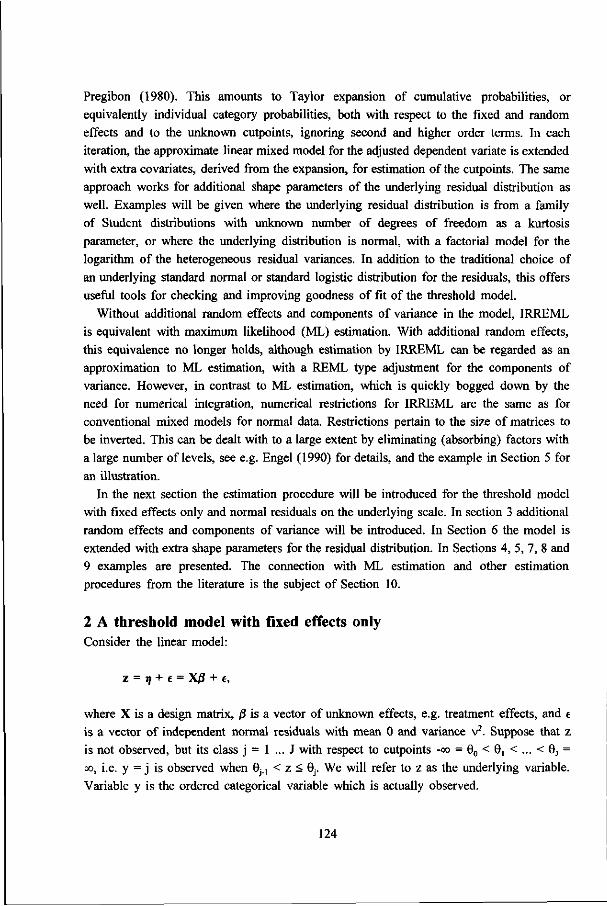
Pregibon (1980). This amounts to Taylor expansion of cumulative probabilities, or equivalently individual category probabilities, both with respect to the fixed and random effects and to the unknown cutpoints, ignoring second and higher order terms. In each iteration, the approximate linear mixed model for the adjusted dependent variate is extended with extra covariates, derived from the expansion, for estimation of the cutpoints. The same approach works for additional shape parameters of the underlying residual distribution as well. Examples will be given where the underlying residual distribution is from a family of Student distributions with unknown number of degrees of freedom as a kurtosis parameter, or where the underlying distribution is normal, with a factorial model for the logarithm of the heterogeneous residual variances. In addition to the traditional choice of an underlying standard normal or standard logistic distribution for the residuals, this offers useful tools for checking and improving goodness of fit of the threshold model.
Without additional random effects and components of variance in the model, IRREML is equivalent with maximum likelihood (ML) estimation. With additional random effects, this equivalence no longer holds, although estimation by IRREML can be regarded as an approximation to ML estimation, with a REML type adjustment for the components of variance. However, in contrast to ML estimation, which is quickly bogged down by the need for numerical integration, numerical restrictions for IRREML are the same as for conventional mixed models for normal data. Restrictions pertain to the size of matrices to be inverted. This can be dealt with to a large extent by eliminating (absorbing) factors with a large number of levels, see e.g. Engel (1990) for details, and the example in Section 5 for an illustration.
In the next section the estimation procedure will be introduced for the threshold model with fixed effects only and normal residuals on the underlying scale. In section 3 additional random effects and components of variance will be introduced. In Section 6 the model is extended with extra shape parameters for the residual distribution. In Sections 4, 5, 7, 8 and 9 examples are presented. The connection with ML estimation and other estimation procedures from the literature is the subject of Section 10.
2 A threshold model with fixed effects only Consider the linear model:
z = if + e = Xß + e,
where X is a design matrix, ß is a vector of unknown effects, e.g. treatment effects, and e is a vector of independent normal residuals with mean 0 and variance v2. Suppose that z is not observed, but its class j = 1 ... J with respect to cutpoints -oo = 0O < 0, < ... < 0j = oo, i.e. y = j is observed when 0j., < z < 0j. We will refer to z as the underlying variable. Variable y is the ordered categorical variable which is actually observed.
124

When several individuals or units correspond to e.g. the same treatment, they may be grouped together. For the i-th group, let n be the number of observations in class j and iij = (nM ... nu)' be the vector of counts, n, follows a multinomial distribution with total N:
= nM + ... + nu and probabilities:
ns = oce;) - o(e;,), j = i... J, 0)
where <I>(.) is the cdf of the standard normal distribution and 0*j = (9j - nf) / v. For ungrouped data n = 0 or 1 and N( = 1 for all i. Both for grouped and ungrouped data, we will refer to i = 1, 2, ... as the units.
When the cutpoints are unknown, without loss of generality, v2 may be fixed at any convenient positive value, typically 1 in this case. Also, when there is an overall mean in ß, one of the cutpoints or the overall mean may be fixed at an arbitrary value. Here, unless stated otherwise, 0, = 0. The cutpoints are collected in a vector £. We will first derive estimating equations for ß for known £. Then, for unknown £, additional estimating equations will be derived for the cutpoints.
2.1 Estimation for known £ In deriving estimating equations we will closely follow the iterative re-weighted least squares algorithm for generalized linear models (GLMs) (see e.g. McCullagh and Neider, 1989, §2.5). The linear combination q = Xß will be referred to as the linear predictor. For the i-th unit: u = N ^ = h^ri,) = h^x^jS), where u is the mean of count n and function h^.) follows from (1). In GLM terminology, functions hjj(.) define an inverse (composite) link function.
Suppose that u , r\{, ... are evaluated for starting values ß0 for ß. Parameter v will be fixed throughout at value 1. An adjusted dependent variate Ç is defined by:
Ç,j = Tlo i + (nu - ^o ij) / tyCrio (; £), (2)
where h^Oi; £) is the derivative with respect to t|. For later use, functional dependence on £ is included in the notation. It is readily shown, see e.g. Engel and Keen (1994), that vector f = (Ç„ ... Çu, Ç2] ... Ç2J, ... ) ' has approximate moments:
E(f) = Xß and Var(f) = R, (3)
where X = X<8>1„ ® is the Kronecker product and lj is a vector of length J with all elements equal to 1. R is a block diagonal matrix with blocks Rj = B^B, along the diagonal. Ej is the covariance matrix of the multinomial distribution for the i-th unit: S, = Nj{diag(7t0 j) - ir0 (ir0 / } , where 7ti = (7in ... % ) ' is the vector of probabilities for that unit. B| is a diagonal matrix with elements hJClo i £)"' along the diagonal. Ej is not a full rank
125

matrix. Generalized inverses of E; are of the form: E; = diag(n 0 y) - T1,1J' with x an arbitrary constant, see McCullagh and Neider (1989, §5.3.3). Parameters ß are updated by weighted regression on Ç After each iteration, f and R are updated for the current estimates for ß solved from the normal equations:
XRXß = X'R-f. (4)
Because the u within a unit sum to the fixed total Nj, equations (4) are independent of the generalized inverse used. Choosing T = 0, it follows that the equations can be set up as if the observations nM ... n^ are independent Poisson counts with means \\u ... \xiy In that case R" will be a diagonal matrix of iterative weights
Wij = hjjOii; if I ns, (5)
similar to an ordinary GLM. The (composite) link function as an inverse of functions hy(.) exists only locally in the neighbourhood of points n with hjj(r|; £) * 0. Points where hy(r|; ij) = 0 are obviously problematic. When, similar to the approach in Thompson and Baker (1981), the adjusted dependent variate is modified by multiplication with h-j(r|; | ) , the regressors, when modified in the same way, become equal to 0. This suggests that offending observations may be ignored in an iteration step. For known cutpoints, the iteration process can be condensed by employing a "pooled" adjusted dependent variate Ç; and "pooled" weights w>:
Q = EWjjÇij / Sw(j = rij + ZlhyOii; ÉX^-u^/vy} / w( and w< = Swy = Zh;/^; £)2 / nÉj. j j j j j
Pooling reduces the number of "observations" Ç and effectively removes problems with 0 derivatives. When cutpoints are unknown, which will be discussed in the next section, pooling is not possible. Note that the model with known cutpoints has some use in practice, for instance when a variable is observed upto the nearest integer.
2.2 Estimation for unknown £ We now have to supply additional estimating equations for the cutpoints in £. In GLM terminology, £ can be regarded as a vector of parameters in the (inverse) link function. An approach similar to Pregibon (1980) (see also McCullagh and Neider, 1989, §11.3) will be used. The means u are linearized with respect to both n, and £ around current values Ti0i and f0:
Hü * Hoij + [dhijOv; k)ldx\^Ao (r|rr)oi) + [ d h ^ ; !)/ö£];oUo (Ho),
which implies that:
126

Tloi + (Hij-Hoij) / hij(îloi, lo) œ Tl, + {[5hij(Tii; ^)/ô{];0i>50 / [ôhij(T|L; £)/örii]noUo}(HoX
and consequently:
E(Çij) « r,ä + { [Ôh^; |)/ô|]'noUo / [ S h ^ ; O / a ^ W A*,
where A£ = £ - ij0- This suggests to extend the set of explanatory variables in the weighted regression for C, with columns of the matrix X4 with elements [dh^r^; i|)/9Çk] / [dh^rij; ÇyôriJ, evaluated for current values »/„ and £0, and with coefficient vector Aif. £ can be updated by: i; = ^0
+^?- This can be combined with the iterations in Section 2.1, updating Xç as a part of X after each iteration. The necessary derivatives are:
ahgOiij «/açk = N ^ Ö O ^ ) ^ ) - (arçev .yau» =
Nj<|)(0*j) when Çk = 9j, -Ni(()(ö*j.]) when t,k = 9j.„ and 0 otherwise, and (6)
ahgOu «/ais =Niwe*ij,)-<|)(e:j)},
where ())(.) is the pdf of the standard normal distribution. Some algebra shows that the combined iterative proces is equivalent to Fisher scoring for
maximising the product multinomial likelihood of counts n . Thus, the final estimates $ and I are ML estimates. The equivalence with ML estimation no longer holds in the next section, where the estimation procedure is extended for additional random effects in the linear predictor ij.
3 A threshold model with additional random effects Now, suppose that the underlying variable follows a linear mixed model:
z = i) + e = Xß + Zu + £, (7)
where Z is a design matrix for additional random effects collected in vector u; u ~ N(0, G). Often G is a blockdiagonal matrix with blocks cr A, ... cr2Ac along the diagonal, where A, ... Ac are known matrices and cr2 ... a2, are unknown components of variance to be estimated from the data. Here, we will assume that A, ... Ac are identity matrices. Again, we start under the assumption that cutpoints in £ are known. Moments in (3) still hold, but conditional upon u. The first two marginal moments of the adjusted dependent Ç variate from (2) are approximately:
E(f) = Xß and Var(f) = ZGZ' + R,
127

where X and R are defined as before and Z = Z®lj. Parameters will be estimated by iterative use of REML, as described in Engel and Keen (1994), i.e. iterative weighted regression from Section 2 will be replaced by iterative weighted REML. After each iteration step, f and R are updated employing current estimates for ß and predictions for u solved from the mixed model equations (see e.g. Engel, 1990):
(8) X'R X
Z'R X
X'R Z N
Z'R Z + G"1, fp) UJ
[X'R" C)
[Z'R- cj
The mixed model equations (8) replace the normal equations (4). They are independent of the generalized inverse R" used. Again, we will choose the diagonal generalized inverse with elements w,j from (5). Components of variance will be updated by one or several steps of the Fisher scoring algorithm for REML, applied to the approximate linear mixed model for Ç with residual weights Wy. Since one step of Fisher scoring, or equivalently one step of Rao's MINQUE (Rao, 1973, §4j.), can be formulated in terms of the solution and bits and pieces of the mixed model equations (see e.g. Engel, 1990), estimates for components of variance are independent of the choice of generalized inverse. In particular it follows that estimates are the same for multinomial or independent Poisson counts. For unknown cutpoints, again Pregibon's method is used to supply the additional estimating equations.
With additional random effects in the model, the estimation procedure is no longer equivalent to ML estimation. However, for given values of the components of variance, estimation of ß and prediction of u is equivalent to maximization of the joint pdf of observations and random effects. This implies that the final estimates ß and predictions û minimize a penalized deviance D + u 'G'u, where D is the deviance of the observations conditional upon the random effects. A similar property holds for IRREML applied to GLMMs, see e.g. Engel, Buist and Visscher (1995). An approximate relationship with ML estimation will be discussed in Section 10. We will now look at two examples, before we extend the threshold model with extra shape parameters.
4 Footshape in lambs The data is reproduced in Gilmour, Anderson and Rae (1987). 2513 lambs are scored in three ordered categories based on the presence of deformities in the feet. Fixed effects correspond to 2 years and 5 strains nested within years. Random effects correspond to 34 sires nested within strains. Sires are assumed to be unrelated. Of interest is the heritability, which is defined as four times the intraclass correlation p = CT2 / (u2,+l) for underlying normal random effects and residuals with v2 = 1.
Results obtained with IRREML and with the marginal approach of Gilmour, Anderson and Rae (1987) are shown in Table 1. Results of the two methods are seen to be very similar.
128

Table 1. Estimates and standard errors for the footshape data. For
coding of fixed effects contrasts Bl, B2 and B3 see Gilmour, Anderson
and Rae (1987)
IRREML Gilmour et al.
Intraclass correlation p 0.056 (0.020) 0.060 (0.019)' Thresholds" 0.374 (0.050) 0.370 (0.052)
1.641 (0.061) 1.603 (0.061)
Effects : Year -0.142 (0.052) -0.139 (0.052) Bl -0.377 (0.077) -0.370 (0.076) B2 -0.316' (0.104) -0.304(0.103) B3 0.099 (0.070) 0.098 (0.070)
' The standard error is a correction of the value 0.144 in Gilmour, Anderson and Rae (1987) (Gilmour, personal communication).
" In Genstat procedure CLASS the first threshold is normally fixed at value 0, but for ease of comparison with the results from Gilmour et al. separate values are calculated fixing the overall mean at value 0.
5 Damage to potato tubers Data result from one of a series of experiments to reduce damage to potato tubers due to a potato lifter. Experiments were performed at the Institute of Agricultural Engineering (IMAG-DLO) in Wageningen, The Netherlands. One source of damage is the type of rod used in the lifter. In the experiment under consideration eight types of rod were compared. It is an emperical fact that degree of damage varies considerably between potato varieties and years. To mimic this variety, two energy levels, six varieties and three weight classes were included in the experiment. Observations were obtained for the combinations of rods, energy levels, varieties and weight classes. Most combinations involved about 20 potato tubers. For some combinations there are no data due to an insufficient number of large potatoes. Two combinations are interchanged, resulting in 40 tubers for the one combination and none for the other. Tubers were dropped from a height determined by the energy level required. To determine the damage, each tuber was peeled and the degree of blue colouring was classified into one of four classes (class 1 for no damage to class 4 for severe damage). Observations in the form of counts per class and combination are reproduced in Table 2.
Of interest are overall differences between rods. Other factors are introduced to create sufficient variety in experimental conditions and are not of primary interest themselves. There is certainly no interest in a detailed description of interaction effects. A pragmatic approach was followed where main effects were introduced as fixed effects and interactions as random effects. This offers a simple summary in terms of main effects, as well as a quick screening device to judge importance of interactions by the size of their
129

Table 2. The potato damage data. Counts n for the four classes from
damage" to "severe damage"
Weight
Var Rod 1 1
2 3 4
5
6 7
8
2 1
2
3 4
5
6 7
8
3 1 2 3
4 5
6 7
8
4 1
2
3 4
5 S 7
8
5 1 2
3 4 5
6 7
8
6 1 2 3 4
5 6 7
8
Energy
class 1
5
a e 2
il
12
8 15
4
8 3
1
16 16 11
10
3 18
5 1
12
16 20 18
4 12
10 2
17
18
19 15
9 17
15 12
16 20
20 20
5
18 5 5
15 19 18
18
14
11 13
9 8
5 12
4
5
3 10
3
3 3
9 10
2 1 7 4 7
3 0 2
9 8
10
8
2 2
1 3
10 2
5 7
4
0
0 0
14 2
14 14
5 1 2 2
1 1
0 6
0 2
0 0
4
0
6 11
1 0
0 0
8 0 4
6 1
0 0
0
7
0 0 4
0 0
0 0
1
0 0 0
0 0
0 0
1
0 0 1 0 0 0
0
.5
0 0 0 3
0 0
0 0
7
0 1
5
0 0
0 0
7
0 4
9 0 1 0
0
0
0 0
6 0
0 0 1
0 0 0 0
0 0
0 0
0 0
0 0 0 0 0
0
(Joule
5 6
5 2
16
15 9 0
5 13
5 0
10 10
11 13
6 12 10
2
16 14 16
16
4
17 10
4
18 19
20 20
10 19 14
7
15 19 17
18
6
18 13
0 16 19 17
15
2
31 11
13 11
4
5 7
0
7
6 12
8
9 7
6 6
8 6 8
6 4
5
3 3
11
2
9 8 2
1 0
0
10 1 6
11
4 1
2 2
13 2 7
15 3 1 3 4
)
2 1
0 6
0 0 3
0
5 1
3 11
1
1 1 0
5 1 0
10 0 0
0 0
3
0 0
6 0
0 0
0
0 0 0 1
1 0
0
0
0 0 0 5 0 0 0
0
1 0
0 0
0 0 1
0
1 0
0 1
0
1 0 0
1 1 2
2 0 0
0 1
1
1 0
1 0
0 0
0
0 0 0
0 0 0
0
0
0 0 0 0 0 0 0
0
0 7
1 4
15 11
11 17
9 18
13 0
16
15 14
12
3 10
8 3
16
15 15 16
10
16 15
5 17
16 17 17
0 0
16
11 0 0
0
0
7 17
8 0 0 0
0 16
3
0 10
19 13
4
4 9 2
7 2
6
9 2
3
5 3
15 6 9
5 3 5 5 4
9 3 4
11
2 2
2 2
0 0
4 8 0
0 0
0
13 3
11 0 0 0
0 4
0 2
0 3
0 0 0 1
2
0 0
9 1
2
1 2
2 2 2
10 0 0
0 0
1 1
0 4
0 0
1 0
0 0 0 0 0
0 0
0
0 0 1 0 0 0
0 0
0 0 0
0 1 5
0 0
0 0 0
2
0 0
0 1
0 2 1
1 1 0
0 0
0 0
0
0 0
0 0
0
0 0 0 0 0
0 0
0
0 0 0 0 0 0
0 0
Energy
2 8
3 0 9
5 9
19
0
6 1
0 6
16 11 11
1 10
2 1
14 11
14 12
0
8 2
1 10 17
15 19
3 9 1
2 16 15
18
19
2 10
7 2 7
17
10 18
1
5 11
7
0
6 12
9
0
5 9 6
3 12
3
6 6
2 5
2 0
5 6 5 4
1
6 2
0
9 0
5 0
9 10
7
4 3 4
0 1
8 10
6 4
10 3 9 2
7
1 4 1
3 1 1
0
6 2 5
3 2
1
0 2
2 2
3 5 0
1 0 0
6 2
6 3
0 0
0 0
6 0
4 3 0 0
1
0
10 0
5 12
1 0 0
0
1
6 0 4
18
0 0 1
0
7
3 7
14
0 0
0 1
15 2
12
13 1
1 1 1
13 2 7
15 0 0
0 0
2 0
5 11
1 0
0
0
0 0 2 2
1 0 0
0
(Joule
2
5 2 0 9
12 5
17
1
5 3 0
7
11 15 13
0 9 2
0 13 15
16 18
0
10 9
0 15 18
20 17
3 8 4 2
17
19 18
19
4 14
2
0 11 18 14
19
2
12 12 10
2
9 6
12 1
4
11 6
1
9 6
2 6
0
2
5 0
5 4
3 2
3
9 11
5 4
2
0 2
11 11 14
3 2
1 1
1
12 6
13 14
8
1 5 1
)
6 3 5
5 1 1
0 0
6 2
6 7 4
3
3 0
4 8
5 2 1
0 0 0
5
0 0
9 1
0 0 0
5 0 2
9 0 0 0
0
4
0 4 6 0 0 1
0
0 0 3
13 0 1
0 0
9 1
5 12
0 0
0 0
16 1
8 18
0 1
0 0
12
0 0
6 0
0 0 0
0 0 0 6
0 0
0 0
0 0 1 0 0 0 0
0
10 4
3 0 0 7
4 19
1 7 7
2
8 14
16 13
2
10 3 1
13
13 12 14
3 12
7
0 16
18 14
20
5 12
7
6 16 17
18 17
3 13
2 4 6
18 15
19
3
7
15 11
2
0 10
4 1
7 12
6 7
11
6 3 7
3 6 5
0 7
5
8 6
7
6
5 1
3 0
4 0
11 8
12 6 4 3
2 2
15 7
18 10 13
2
5 1
3 1 4
14
0 3 1
0
6 1 6
10 1
0 0 0
9 4
9 7
0 0
0 0
8 0
5 10
1 1
2 0
4
0 1 6 0 0
0 0
2 0 0 6 1 0
0 0
0 0 2 4
0 0
0 0
6
0 1 1
0
0 0 0
6 0 2
12
0 0 0 0
2
1
2 8
0 0
0 0
0 0
0 2 0 0
0 0
0 0 0 0 0 0 0
0
130

Table 3. Components of va r iance for the po ta to damage da ta
I n t e r a c t i o n term component ( s . e . )
rod .energy 0.120 (0.073) r o d . v a r i e t y 0.074 (0.031) r od .we igh tc l a s s 0.042 (0.022) e ne rgy .va r i e t y 0.003 (0.010) energy .weigh tc lass 0.013 (0.016) v a r i e t y .we i gh t c l a s s 0.011 (0.011) r od . ene rgy . va r i e t y 0.039 (0.023) r od . ene rgy .we igh tc l a s s ' r o d . v a r i e t y .we i gh t c l a s s ' e n e rgy . va r i e t y .we igh t c l a s s ' r od . ene rgy .va r i e t y .we igh t c l a s s 0.055 (0.024)
' Negative e s t ima tes (are rep laced by 0 .0001) .
corresponding components of variance. Normal distributions were assumed with residual variance v2 = 1. Four-factor-interaction effects were absorbed when solving mixed model equations (8). Estimated cutpoints (standard errors in parentheses) are 0 (fixed), 1.41 (0.03) and 2.30 (0.04). Estimated components of variance are shown in Table 3. Estimated rod effects as differences with rod number one are:
Rod: 1 2 3 4 5 6 7 8 0 -1.26 -0.42 0.55 -1.50 -1.85 -1.76 -2.09.
Standard errors of differences are approximately 0.43. Estimates in Table 3 show that the larger components involve interactions with rods. Estimated rod effects are therefore less precise than e.g. estimated variety effects (standard error of difference about 0.20). Despite the larger standard errors it may be concluded e.g. that rods 1, 2, 3, 4 are worse than rod
6 Extending the threshold model So far residuals were assumed to follow a normal distribution, corresponding to a probit link for probabilities P(yj < j | u) = vj/y. Other popular choices are the logistic distribution and extreme value distribution. For the logistic distribution, with v2 = iz2/3, the link function is the logit link:
logit(Vij) = log^/O-Yij)) = 8j - rij.
131

For the extreme value distribution, with v2 = 1, the link function is the complementary log-log link:
log(-log(l-Vij)) = Gj - Tl,
These alternatives, for models with fixed effects only, are discussed in some detail by McCullagh (1980) and referred to as the proportional odds and proportional hazards model respectively.
We will now introduce more general link functions, or underlying distributions, allowing for additional unknown (shape) parameters. Let the cdf of the underlying variable z from (7), conditional upon the random effects u, be F((z-n)/v; X), where X is a vector of additional shape parameters. Let f(x) = F'(x; X) be the derivative with respect to x. A useful family of distributions, as a robust alternative to the standard normal distribution, is the family of Student distributions: f(x) = y[QJ(k-2))fx{yfQJ(X-2))x), for X > 2 and f(x) = fx(x) for 0 < X < 2, where fx(.) is the pdf of Student's distribution with X degrees of freedom. For use of the Student distribution in statistical inference see e.g. Fraser (1979). Usually n and v2 will be the (conditional) mean and variance of z, although these moments do not necessarily have to exist, e.g. for the Cauchy distribution (Student distribution with X = 1) where f(x) = 1 / {7t(l+x2)}. Typically X is assumed not to depend on the experimental units.
In addition to TJ, V2 may be modelled in terms of explanatory variables as well:
gO2) = Vv = Xv7-
Here, g(.) and i/v are the link function and linear predictor for the variance. ^ is a design matrix and y a vector of fixed effects for the variance. An obvious choice for g(.) is the logarithmic link, see e.g. Aitkin (1987) and McCullagh and Neider (1989, §5.2.2 and Ch.10).
Extra shape parameters are added to vector £ and estimating equations are derived once again by Pregibon's method. Derivatives in Xç can be evaluated using the following results:
dti^K i)idt,k = HKSFO'J ; x)/dçk) - (aF(e*J.,; xyau)},
ahijOu D/Srii = N^fO'j.,; X) - f&\, X)} / v.
Consider for example parameters y in the variances v2:
5F(e;; X)/dyk = (ÔF(G*j; X)/dv2Xdv2/ônvi)(dnvj/ayk) = - t t f^ ; X) 9^ xvi,k / {g'(v?) v2}.
For the log link, elements of X4 are of the form:
132

•/2xvi,k {f(e;; xxQ^-m]^ xxe^wiW'ï x) - f(e;,; x)}.
For a single shape parameter X, it may be more convenient to fit the model for a grid of values for X, and inspect the results. For the cutpoints, the following reparameterisation may be convenient: 6, = 0, 02 = exp^) , 93 = exp(5,) + exp(52), ... . Elements for Sk in X4 are of the form: f(0*j; X) exp(ôj.,) / {f^; X) - f(8*j.,; X)}, when 1 < k = j -1 , or exp(ôk), when 1 < k < j - 1 , and 0 otherwise.
Table 4. Results of 50 simulations
Results for treatment contrasts on the underlying scale:
i/ = 1 v free
Contrast True Average s.d. Average s.e. Average value of sims. of sims.
s .d. Average s.e.
2 - 1
3 - 1
4 - 1
0
1
1
0.09 0.79 0.69
0.23 0.13 0.17
0.21 0.21 0.21
-0 .01 1.04 1.01
0.36 0.19 0.32
0.35 0.25 0.37
Resul t s for e s t imated v±'s (v1 f ixed a t 1 ) :
Treatment True va lue Average s .d . Average s . e .
2
3
4
2
1
2
2.02 1.00 1.98
0.36 0.21 0.42
0.40 0.19 0.42
To illustrate the scope for improvement obtained by simultaneous modelling of r| and v2, a modest simulation was carried out. Data was generated from four normal distributions, representing e.g. four treatments. Combinations of r| and v were (1, 1), (1, 2), (2, 1) and (2, 2) respectively. The sample size was 50 in each case. Cutpoints were -1, 0, 1 and 2. Estimated differences in means with respect to treatment 1 for homogeneous v2 (fixed at value 1) and for heterogeneous v2 (v2 fixed at value 1 for treatment 1 and estimated for treatments 2, 3 and 4) are presented in Table 4. In the table average differences over 50 simulations, corresponding standard deviations as estimated from the 50 simulations and the average of the 50 standard errors for the treatment contrasts produced by Genstat are shown. The latter standard errors are based on Fisher information under normality for the
133

adjusted dependent variate. Estimated treatment contrasts are seen to be fairly unbiased when heterogeneity is taken into account. Note that the standard deviations estimated from the 50 simulations and the averages of the standard errors from Genstat are in reasonable agreement. Also shown are some results for the estimated v's. Again, estimates are fairly unbiased and estimated standard errors on average are quite acceptable. We will look at three examples of the extended model.
7 Therapeutic effect of nootropic agents This example is from Uesaka (1993), who used it for illustrating a test for interaction between two treatments and a block factor based on logarithmic generalised odds ratios. The data is from a multicenter trial on the therapeutic effect of two nootropic agents on patients with multi-infarct disease. The effect was evaluated on an ordinal scale of five categories and patients were classified a posteriori into four groups according to the baseline severity of overall neurological symptoms. Likelihood ratio test statistics (which may be referred to an appropriate chi-square distribution) for treatment effects and interaction, for different underlying distributions fitted to the fixed effects model are presented in Table 5, along with the residual deviance as a measure of goodness of fit.
Table 5. Therapeutic effect of nootropic agents. Likelihood ratio
statistics for treatment main effects and interaction and mean
déviances for various models fitted to the data
Distribution
normal logistic extreme value
left skew right skew
lognormal Student
1 df 2 df 3 df 5 df 8 df
20 df
Likelihood ratio statistics
Main effects (1 df)
3.0 2.5
2.7 no convergenc
2.3 converges to no convergenc
1.6 1.9 2.3 2.5 2.8
Interaction (3 df)
4.4
4.7
4.4 e
4.0 the normal e
4.8 4.8 4.8 4.7 4.5
distribut
Mean deviance
0.85
0.88
1.19
0.85 ion (df = <»)
1.00 0.96 0.91 0.88 0.86
134

This illustrates that there is little evidence for the existence of a treatment main effect or interaction between treatment and baseline severity. Use of the normal distribution may indicate a treatment effect, but this effect is not robust for the choice of underlying distribution.
8 Severity of nausea in chemotherapy Data on the severity of nausea (in 6 ordered categories from "none" to "severe") experienced by 219 patients with cancer while undergoing chemotherapy, is taken from Farewell (1982). Patients were classified as to whether their chemotherapy included or did not include cisplatin. Farewell introduces overdispersion by allowing a random shift of the cutpoints for each patient. Within a patient all 0's are shifted by the same amount, i.e. shifts can also be considered as random main effects u for patients. Farewell starts with a proportional hazards model and conveniently assumes that exp(u) is from a gamma distribution. This allows the u's to be integrated out of the probabilities n for severity of nausea. The likelihood is optimized over a grid of values of the index parameter c of the gamma distribution. The mean deviance for the extreme value distribution, without the u's (c = oo), is 2.91 on 4 degrees of freedom (10 parameters for the saturated model minus 6 for the threshold model) and the proportional hazards model is rejected at the 0.05 level employing the likelihood ratio test with a chi-square distribution on 4 degrees of freedom. For the normal distribution the mean deviance is 1.99, for the logistic distribution: 1.65 and for the Student distribution with X = 1 (Cauchy distribution): 0.45. Neither distribution leads to rejection of the model by the likelihood ratio test on either 3 or 4 degrees of freedom at the 0.05 level. For Farewells model with random shifts (c = 1), the mean deviance is 1.60 on 3 degrees of freedom. The ratios of the ML estimates for the cisplatin effect ß and its estimated standard error (ignoring variability in additional paramaters, i.e. X for the Student distribution and c for Farewell's model) on the underlying scale for the Student (X = 1), normal and logistic distribution and Farewell's overdispersion model are 3.6, 3.3, 3.3 and 3.9 respectively. Although Farewell did not intend to present a general model for ordinal data, and only used the example as an illustration of the random shift model, it can be concluded that an improved fit can just as easily be obtained by a change of residual distribution (or link function for cumulative probabilities) as by introduction of variability in the cutpoints. Note that when patient and residual effects on the underlying scale are from the normal distribution, they can be pooled and the model remains essentially the same. A similar result approximately holds for normal and logistic effects as well.
9 Damage to potato tubers, continued As a point of interest the assumption of a common residual variance on the underlying scale was checked. Adding dependence of v2 on type of rod results in the following estimates for v: 1 (fixed), 0.90 (0.06), 0.86 (0.05), 0.76 (0.04), 0.89 (0.07), 1.09 (0.09), 0.85 (0.07) and
135

1.00 (0.10) for rods 1 to 8 respectively (standard errors in parentheses). Comparisons may be made on the log scale. However, allowing for heterogeneity does not entail important changes in conclusions about the differences between rods.
10 Discussion McCullagh (1980) discusses the fixed effects threshold model. Thompson and Baker (1981) show how these models can be fitted into the GLM framework for ML estimation. ML estimation for threshold models with normal random effects, employing numerical integration by Gauss-Hermite quadrature (Abramowitz and Stegun, 1965, p.924), is presented in e.g. Jansen (1990, 1992). Iterative re-weighted REML is more akin to quasi-likelihood estimation. Estimation only depends on the first two moments and no full distributional assumptions are needed. When for grouped data the residual variance in the mixed model for the adjusted dependent variate is not kept at a fixed value, it may represent an additional multiplicative under- or overdispersion parameter with respect to the covariance matrix of the multinomial distribution (McCullagh and Neider, 1990, §5.5). Application of GLMM methodology to the one-threshold model (J = 1) for binomial data is discussed in Engel, Buist and Visscher (1995). They show that the estimate for the additional dispersion parameter may be expressed in terms of Pearson's chi-square statistic evaluated for predicted random effects with an "effective" number of degrees of freedom estimated from the data.
In the context of animal breeding, Gianola and Foulley (1983) present a Bayesian approach to inference about ß, u and 8 = (0, ... 0,.,)' for known components of variance. The aim is to evaluate animals on the basis of their predicted genetic merit û. Thresholds and fixed effects are nuisance parameters. Vague priors for 6 and ß and a normal prior density for u are assumed, ß, u and 0 are estimated by the mode of their joint posterior density, i.e. by the values that maximize the joint pdf of y and u. Maximization is by Fisher scoring. Some algebra shows that this is equivalent to the use of equations (8) extended with the covariates in Xç for Ai- = A0 as following from Pregibon's correction. The Bayesian procedure presented in Harville and Mee (1984) is equivalent to Gianola and Foulley (1983), but also includes estimation of components of variance. See in this respect also Foulley, Im, Gianola and Hoeschele (1987). An update of the components of variance can be shown to correspond to one step of an EM algorithm for conventional mixed models applied to the adjusted dependent variate Ç, see e.g. Engel, Buist and Visscher (1995). This solves the same set of final estimating equations as the Fisher scoring algorithm for REML employed in this paper.
Optimization of the joint pdf of y and u is the basic principle behind the estimation procedure suggested by McGilchrist (1994). McGilchrist presents three possible estimators for the components of variance referred to as: BLUP, ML and REML estimators. The REML estimators are of the EM type, similar to estimation of the components in Harville
136

and Mee (1984) and Foulley, Im, Gianola and Hoeschele (1987), and equivalent to the IRREML estimators.
For normally distributed random effects u, IRREML estimates ß and predictions û are maximum hierarchical likelihood estimates, according to the definition by Lee and Neider (1996) of hierarchical likelihood (h-likelihood) as the logarithm of the joint pdf of y and u. Use of the h-likelihood is motivated by Laplace integration. For Laplacian integration in nonlinear mixed models see also Wolfinger (1993) and for GLMMs Breslow and Clayton (1993). In the discussion of Lee and Nelder's paper, the relationship between maximum h-likelihood and ML estimation is commented upon by Engel and Keen (1996). These comments include estimation of components of variance by maximum adjusted profile h-likelihood estimation in relation to ML estimation, and cover the present case of ordinal data as well.
Estimation as presented in Gilmour, Anderson and Rae (1987) is a generalization of their approach for one-threshold models (Gilmour, Anderson and Rae, 1985) for an underlying standard normal distribution. There is a strong similarity to IRREML, except that their adjusted dependent variate and weights are expressed in terms of marginal rather than conditional moments with respect to u. A comparison, which includes extensive simulation results, between the marginal and conditional approaches for the one-threshold model is presented in Engel, Buist and Visscher (1995). The example about foot shape in lambs in Section 4 offers a numerical comparison.
Since the fixed effects ß are introduced on the same underlying scale as the random effects u, the model is subject specific in the terminology of Zeger, Liang and Albert (1988). The interpretation of effects ß is in terms of conditional probabilities and not in terms of marginal probabilities. The latter follow by integrating out the random effects. In the threshold model, with F(.) equal to the cdf of the normal distribution, v2 = 1 and u ~ N(0, G), marginal effects on the probit scale follow by shrinking elements of ß by a factor (l+u]+...+aly'À. When F(.) is the cdf of the standard logistic distribution and v2 = 7i2/3, for the marginal probabilities, the logit scale holds only approximately, and an approximate shrinkage factor may be derived from the close connection between the normal and logistic distribution, see e.g. Engel, Buist and Visscher (1995). In general, expressions for marginal effects may be derived by Taylor series expansion, see Engel and Keen (1994).
Approximation by Laplace integration is not sufficiently accurate for estimation of components of variance when the amount of information per individual random effect is low, irrespective of the number of random effects. Simulation results in Engel, Buist and Visscher (1995) show that in that case IRREML does not perform well for the one-threshold model for binary data. A similar result can be expected for thresholds models for ordinal data. The chemotherapy data in Section 8 offer an extreme example. The threshold model with an underlying extreme value distribution for the residuals and random normal patient effects is, in view of the similarity between the lognormal and the gamma distribution, an obvious contender to Farewell's random shift model. IRREML produces an
137

estimated cisplatin effect of 0.32, with an estimated standard error of 0.20. This suggests that cisplatin has no significant effect, in contrast to the various models fitted in Section 8, which is undoubtedly a consequence of the fact that to each shift u there corresponds only one ordinal observation. When the u's are integrated out, resulting in a link function with additional index parameter c, the algorithm from Section 2 can be applied.
Acknowledgements Thanks are due to Joop de Bree, Cajo ter Braak and two referees for critical comments on earlier versions of the manuscript. The dataset on potato tubers was kindly provided by Jan Huijsmans.
References Abramowitz, M, Stegun, I. (1965). Handbook of mathematical functions. Dover, New
York. Breslow, N.E., Clayton, D.G. (1993). Approximate inference in Generalized Linear Mixed
Models. Journal of the American Statistical Association 88, 9-25. Engel, B. (1990). The analysis of unbalanced linear models with variance components.
Statistica Neerlandica 44, 195-219. Engel, B., Buist, W., Visscher, A. (1995). Inference for threshold models with variance
components from the generalized linear mixed model perspective. Genetics Selection Evolution 27, 15-32.
Engel, B., Keen, A. (1994). A simple approach for the analysis of generalized linear mixed
models. Statistica Neerlandica 48, 1-22. Engel, B., Keen, A. (1996). Contribution to the discussion of Lee and Neider (1996).
Hierarchical Generalized Linear Models. Journal of the Royal Statistical Society B 58, 656-657.
Farewell, V.T. (1982). A note on regression of ordinal data with variability of classification. Biometrika 69, 533-538.
Foulley, J.L., Im, S., Gianola, D., Hoeschele, I. (1987). Empirical estimation of parameters
for n polygenic binary traits. Genetics Selection Evolution 19, 197-224. Fraser, D.A.S. (1979). Inference and linear models, McGraw-Hill, New York. Genstat 5 committee (1993). Genstat 5 Release 3 Reference Manual. (R.W. Payne
(Chairman) and P.W. Lane (Secretary)). Clarendon Press, Oxford. Gianola, D., Foulley, J.L. (1983). Sire evaluation for ordered categorical data with a
threshold model. Genetics Selection Evolution 15, 201-223. Gilmour, A.R., Anderson, R.D., Rae, A.L. (1985). The analysis of binomial data by a
generalized linear mixed model. Biometrika 72, 593-599. Gilmour, A.R., Anderson, R.D., Rae, A.L. (1987). Variance components on an underlying
scale for ordered multiple threshold categorical data using a generalized linear mixed
138

model. Journal of Animal Breeding and Genetics 104, 149-155. Harville, D., Mee, R.W. (1984). A mixed model procedure for analyzing ordered categorical
data. Biometrics 40, 393-408. Jansen, J. (1990). On the statistical analysis of ordinal data when extra variation is present.
Applied Statistics 39, 75-84. Jansen, J. (1992). Statistical analysis of threshold data from experiments with nested errors.
Computational Statistics and Data Analysis 13, 319-330. Keen, A. (1994). Procedure CLASS, GLW-DLO Procedure Library Manual, Release 3[1]. Lee, Y., Nelder, J.A. (1996). Hierarchical Generalized Linear Models (with discussion).
Journal of the Royal Statistical Society B 58, 619-678. McCullagh, P. (1980). Regression models for ordinal data (with discussion). Journal of the
Royal Statistical Society B 42, 109-142. McCullagh P., Neider, J.A. (1989). Generalized linear models, 2nd. ed. Chapman and Hall,
London. McGilchrist, C.A. (1994). Estimation in generalized mixed models. Journal of the Royal
Statistical Society B 56, 61-69. Patterson, H.D., Thompson, R. (1971). Recovery of inter-block information when block
sizes are unequal. Biometrika 58, 545-554. Pregibon, D. (1980). Goodness of link tests for generalized linear models. Applied Statistics
29, 15-24. Rao, C.R. (1973). Linear statistical inference and its applications, 2nd ed. John Wiley,
New York. Schall, R. (1991). Estimation in generalized linear models with random effects. Biometrika
78, 719-728. Thompson, R., Baker, R.J. (1981). Composite link functions in generalized linear models.
Applied Statistics 30, 125-131. Wolfinger, R. (1993). Laplace's approximation for nonlinear mixed models. Biometrika 80,
791-795. Zeger, S.L., Liang, K.Y., Albert, P.S. (1988). Models for longitudinal data: a generalized
estimating approach. Biometrics 44, 1049-1060.
139

Chapter 8
Bias reduction of heritability estimates in threshold models
Submitted for publication.
The simulation study from Chapter 6 for threshold models for
binary data is extended and two methods for bias-correction are
studied.

Bias reduction of heritability estimates in threshold models
Bas Engel' and Willem Buist2
'DLO Agricultural Mathematics Group (GLW-DLO) P.O. Box 100, 6700 AC Wageningen, The Netherlands
2DLO Institute for Animal Science and Health (ID-DLO) P.O. Box 65, 8200 AD Lelystad, The Netherlands.
Summary Penalized quasi-likelihood and iterated re-weighted REML estimates for heritability (or intra-class correlation) in threshold models for binary data with extra random components can be seriously biased. Recent approaches to correct for this bias are studied by simulation, with emphasis on animal breeding models for binary data. Scope for reduction of bias is found to be slim, because of the commonly large number of fixed effects in animal breeding models. Minimal dimensions for the data are identified, such that bias and root mean squared error are of modest size, and useful inference on heritability (or intra-class correlation) is feasible.
Keywords: binary data, threshold model, heritability, bias, mixed model, REML, PQL
1 Introduction A threshold model for binary or binomial data with fixed and random effects and associated components of variance can also be presented in the form of a generalized linear mixed model (GLMM) or a hierarchical generalized mixed model (HGLM). General estimation procedures for GLMMs and HGLMs proposed by Schall (1991), Breslow and Clayton (1993) (penalized quasi-likelihood or PQL), Engel and Keen (1994) (iterated re-weighted REML or IRREML), McGilchrist (1994) (the method referred to as the REML approach) and Lee and Neider (1996) (maximum adjusted profile h-likelihood or MAPHL), and the Bayesian maximum a posteriori (MAP) approach proposed by Gianola and Foulley (1983) and Harville and Mee (1984) are equivalent for threshold models for binary data (see Engel, Buist and Visscher, 1995; Keen and Engel, 1996). All these methods avoid the problem of high dimensional numerical integration in evaluation of the likelihood (or a posterior distribution). Basically, all of them, implicitly or explicitly, involve a normal approximation of the distribution of the random effects conditional upon the observations, which can be motivated by Laplace integration, see Lee and Neider (1996), Engel and Keen (1996) and for MAP: Foulley, Im, Gianola and Hoeschele (1987). That the same estimating equations
143

can be derived in many different ways suggests that MAP / PQL / IRREML / MAPHL is a proper method for estimation of components of variance, intra-class correlation or heritability in threshold models for binary data. Unfortunately, simulation studies (e.g. Gilmour, Anderson and Rae, 1985; Engel et al., 1995) show that estimates so obtained can be seriously biased. Gilmour et al. (1985) were the first to observe bias problems. They studied a simple one-way model, e.g. a sire model with unrelated sires, with m offspring per sire, and with a binary observation per offspring. On the underlying scale, normal distributions were assumed for the independent genetic sire effects and the residual effects, with an overall mean as the only fixed effect. The simulation results suggest that with MAP / PQL / IRREML / MAPHL the sire variance is underestimated approximately by a factor (m-1) / m, irrespective of the number of sires. Informal arguments for this factor are given in Thompson (1990) and Engel et al. (1995). In more realistic models with more fixed effects and varying family sizes, bias is of a more complex nature, and positive bias may occur as well, depending on the number of observations per fixed effect, as found by Engel et al. (1995).
For small family sizes (small numbers of binary observations per random effect, in a more general formulation), variance and heritability estimates may seriously err, even when the number of families (the number of random effects) is very large. Reduction of this bias is paramount in animal breeding, where a poor heritability estimate will give a wrong impression of potential genetic gain under selection and may affect estimated breeding values (i.e. predictions for individual genetic random effects used in selection). Breslow and Lin (1995) proposed a bias correction for PQL estimates for a variance component in GLMMs. In this paper the performance of this correction applied to heritability estimates in a sire model for binary data is studied by simulation and compared with another method, presented in Engel et al. (1995), based on a change of iterative weights in IRREML. Minimal dimensions are identified for the data, such that useful inference on heritability or intra-class correlation is feasible.
2 Bias correction Although, for convenience, notation for a sire model is adopted, the formulae presented apply to an animal model (see e.g. Henderson, 1984, Ch.22) with a general additive relationship matrix as well. Vector r of values for the liability on the underlying scale is expressed as:
r = Xj8 + Zu + e = ij + €. (1)
Here, ß and u are vectors of p fixed effects (for e.g. combinations of herds, years and seasons: HYS effects) and q random sire effects, respectively, u _ N(0, Aa|), where A is
144

the (known) additive genetic relationship matrix and cr| is the (unknown) sire component of variance. X and Z are design matrices, i; is the linear predictor in the corresponding GLMM. Independent residuals in vector t follow a standard normal distribution. A positive value for the liability of an offspring of a sire corresponds to an observation y = 1, and a negative value to y = 0. Conditional upon sire effects, mean and variance are: E(y | u) = u. and Var(y | u) = V(u) = u(l-u), where u is a conditional probability for e.g. an offspring to be alive at a certain age in a mortality study, denoted by u for the j-th offspring of the i-th sire, and V(.) is the (conditional) variance function.
The bias correction factor in Breslow and Lin (1995) is derived for small values of the variance component for a GLMM with a canonical link function and independent normally distributed random effects. For a sire model for binary data this implies a logistic distribution for the residuals, i.e. cdf L(e) = 1 / (l+exp(-e)), and normal genetic effects for unrelated sires, i.e. A is an identity matrix. To extend the correction factor to related sires, the random part Zu of (1) is written as: (ZL)(L"'u) = Zû. L is a lower triangular matrix such that LL' = A, see Quaas (1976) and Henderson (1976). Elements of fl are independent and we just have to replace design matrix Z by Z in expressions for the correction factor. The corrected variance estimator is: ô | „ = f ô\, where ô\ is the MAP / PQL / IRREML / MAPHL estimator, and factor f follows from:
f = a / (a+b), (2) where
a = lq'(L'Z'W0ZL)(2) lq / 2 = trace(Z'W0ZAZ'W0ZA) / 2 and
b = [lq'(L'Z')(2»{W2 - W1X(X'W0X)-'X'W,}(ZL)<2» lq] / 4.
lq denotes a q x 1 vector of ones. For any matrix M with elements m , M<2) is the matrix with elements m2j, i.e. the direct (Hadamard) product of M with itself. W0, W, and W2 are diagonal matrices with elements noij(l-u0ij), n0ij(l-u0ij)(l-2n0jj) and Ho,ij(l- o,ij)(6u2
0ij-6|i0ij+l), respectively. (J.oij is fXjj evaluated for the estimated fixed effects and sire effects replaced by 0, i.e. ;*„ = (l+exp(-X$))"' for logistic residuals. To a close approximation (Johnson and Kotz, 1970, p6): L(ct) = O(t), where O is the cdf of the standard normal distribution, and c = (15/16)roV3. This implies that (2) approximately holds for normal residuals as well, with fi0 = 0(X$).
In the simple sire model of Gilmour et al. (1985), discussed in the introduction, a = qm2(i20(l-n0)
2/2, b = - qm|io(l-u0)2/2 and f = a / (a+b) = m / (m-1), which is an encouraging
result. For a more realistic model we take resort to simulation, extending studies reported in Hoeschele and Gianola (1989) and Engel et al. (1995), involving an unbalanced sire model for binary data with a relatively large number of fixed effects. Sire effects and residual effects are generated from normal distributions, since this is a more familiar choice than the combination of normal and logistic distributions.
145

In Engel et al. (1995) use of the following alternative iterative weights in IRREML is suggested:
w0 = {g'(u)2 E(V(u))}-\ (3)
where g' is the derivative of the link function g. Both from the corrected component â|>corr and from the IRREML estimate with weights
w0, estimated heritabilities will be calculated. For a sire model the heritability h2 is:
h2 = 4 a2 / (a2s+l) = 4p,
where p is the intra-class correlation on the underlying scale.
3 The simulated data The fixed HYS effects are initially sampled from a N(0, CJ YS) distribution. For each HYS combination a sire has 0, 1 or 2 offspring with probabilities 1 - p^s , pHYS / 2 and pHYS / 2 respectively. Values for pHYS are 0.025, 0.05, 0.10, 0.20, 0.25 and 0.30. The HYS effects and design for sires and offspring are generated only once, after which the same HYS values and the same design are used in all subsequent simulations. Other fixed effects are sire group effects: 4 groups with effects -0.40, -0.15, 0.15 and 0.40. The number of fixed effects p is either 139 (= 135 HYS + 4 sire groups), 38 (= 34 + 4) or 1 (just an overall mean). Independent sire effects are sampled from a N(0, o|) distribution, where a\ = h2/(4-h2) and h2 = 0.25. The number of sires q is either 50 (12, 14, 13 and 11 for the sire groups) or 200 (48, 56, 52 and 44 for the sire groups). For p = 139 fixed effects, simulation results for q = 100 sires (24, 28, 26 and 22 for the sire groups) were collected as well. Residuals are from a N(0, 1) distribution. The overall constant on the underlying scale is: -O"'(P0) (l+o"2
HYS+a|)0'5, where ?o = 0-90 is the overall incidence. The proportion of variance explained by the HYS effects, CT2
HYS / (1+CT2HYS+CT2
S) = o2HYS / (a
2HYS+(4/(4-h2)) = 0.30 for h2
= 0.25. Calculations are performed with Genstat 5 (1993), employing procedure IRREML (Keen, 1994). Expression (2) simplifies, since for the simulation
a = E {S ^(l-Mcij)}2 / 2 and b = [I Z M ^ M ^ V ^ + l ) - d'X(X'W0X)-'X'd] / 4, i j ' j
where d is a vector with elements u0ij(l-u0ij)(l-2u0ij). The alternative weights from (3) are:
w0 = <Kn)2 / {P(l-P) - p «H".)2},
where <|> is the pdf of the standard normal distribution, P = P(y=l) = 0(r|.) is the marginal probability and n* = x'ß I \f(l+o\) is the marginal linear predictor.
146

4 Simulation results Simulation results for heritability based on 200 runs for each parameter configuration are shown in Table 1. Results without correction (bold face in the table) will be discussed first. Within each column, when the average number m of observations (offspring) per random effect (sire) increases (going from bottom to top in the table), the absolute bias and root mean squared error decrease. The bias vanishes, which agrees with consistency for p and q fixed and m -> oo. Within a row, when the number of fixed effects q is reduced from 139 to 38 to 1, or the number of sires p is increased from 50 to 200, the bias starts with a
ble 1 Simulation results for heritability. Bias and root mean squared error are expressed as a percentage of the true value,
ults in the form: bias (s.e. bias) / root mean squared error. First line is the uncorrected result (bold face), second line is the
lit after use of the correction factor, third line is the result with the alternative weights. Heritability h2 = 0.25. Incidence P0 =
). Number of fixed effects p is 139, 38 or 1. Number of sires q is 50, 100 (p = 139 only) or 200. Number of offspring per sire
1, 51, 41, 20, 10, 5 (pHYS = 0.30, 0.25, 0.20, 0.10, 0.05, 0.025). The total number of observations within a row is about the
e for the same number of sires, e.g. in the first row for q = 50 both for p = 139, 38 and 1: m = 60.75.
1er of Kl HYS cts p
er of s q 50 sires
er of pring sire n )
139 fixed effects
100 sires
38 fixed effects overall fixed constant only
200 sires 50 sires 200 sires 50 sires 200 sires
14.5 (3.6)/ 52.2 0) 17.8 (3.6)/ 54.5
1.1 (3.1)/ 44.3
15.0 (3.7)/54.1 5) 18.7 (3.8)/56.7
3.6 (3.2)/45.1
35.0 (4.1)/ 67.8 0) 41.0 (4.3)/ 73.0
22.0 (3.6)/ 55.3
68.4 (7.3)/123.2 83.4 (7.91/138.7 61.9 (7.5J/122.1
241.0(15.1)/321.9 5) 306.6(17.5)/393.5
341.9(22.6)/460.4
508.4(20.41/584.3 25) 660.1(23.61/739.4
543.1(45.5)/594.2
5.1 (2.0)/ 28.7 7.8 (2.1)/ 30.0
-3.6 (1.7)/ 24.7
5.9 (2.1)/ 30.2 9.3 (2.2)/ 32.5
-2.4 (1.8)/ 25.6
5.0 (2.11/ 30.6 9.0 (2.2)/ 32.5
-1.7 (1.9)/ 27.3
34.6 (4.5)/ 72.2 47.1 (4.9)/ 83.4 35.3 (4.4)/ 71.1
96.1 (7.4J/142.3 126.6 (8.55/174.3 118.0 (9.0J/173.2
288.0(13.6)/346.0 387.6(16.1)/449.3
-(*)
•2.1(1.4)/ 19.2 0.4(1.4)/ 19.5
-7.8(1.2)/ 18.5
-1.7(1.4)/ 20.1 1.3(1.5)/ 20.6
-6.1(1.3)/ 18.6
•2.2(1.7)/ 23.4 1.6(1.7)/ 24.2
-5.6(1.5)/ 21.5
3.1(2.5)/ 35.7 10.7(2.7)/ 39.7 6.9(2.4)/ 34.8
28.4(4.8)/ 73.6 50.0(5.6)/ 92.9 52.2(5.41/ 91.8
0.5 (3.1)/ 44.1 3.2 (3.21/ 45.3
-7.8 (2.81/ 39.6
-6.2 (2.9)/ 40.7 -3.1 (2.91/ 41.6
-12.8 (2.61/ 38.4
5.7 (3.1)/ 44.2 9.9 (3.21/ 46.6 1.8 (2.91/ 41.2
8.3 (4.7)/ 67.3 16.2 (5.1)/ 73.4 5.0 (4.6)/ 65.7
48.1 (9.D/136.7 74.3(10.6)7166.4 63.6(10.11/155.5
104.0(7.4)/147.3 143.7(13.4)/237.5 161.0(9.21/206,7 214.6(16.71/318.3
-(*) 204.7(16.91/312.5
-4.2(1.2)/ 18.0 -1.9(1.3)/ 18.0 -8.4(1.1)/ 17.8
-5.4(1.4)/ 20.2 -2.4(1.4)/ 20.2 -6.7(1.3)/ 18.8
•9.7(1.7)/ 25.8 -6.0(1.8)/ 25.5 -8.6(1.5)/ 23.1
•9.0(2.2)/ 32.6 -2.4(2.4)/ 33.6 2.5(2.2)/ 31.4
•6.5(3.8)/ 53.9 7.7(4.31/ 61.7
24.6(4.51/ 68.1
•10.9(4.91/ 70.4 12.5(6.2)/ 87.8 31.7(6.7)/100.1
•4.2(2.5)/ 35.3 -2.8(2.51/ 35.7
-12.3(2.11/ 31.9
•6.9(2.6)/ 37.0 -5.2(2.61/ 37.4
-13.2(2.21/ 33.9
-7.4(2.9)/ 41.0 -5.3(2.91/ 41.5
-11.6(2.51/ 37.3
•9.0(3.6)/ 51.5 -5.1(3.7)/ 53.0 -6.5(3.3)/ 46.8
•12.8(5.2)/ 73.9 -5.8(5.6)/ 78.5 4.5(5.6)/ 78.5
-22.3(6.4)/ 93.0 -10.9(7.35/103.0 11.0(8.35/118.0
-4.9(1.2)/17.0 -3.5(1.25/16.8
-11.8(1.01/18.3
•9.1(1.2)/18.6 -7.4(1.2)/18.1
-14.2(0.9)719.4
-9.4(1.45/21.6 -7.3(1.41/21.1
-12.0(1.15/20.1
-13.7(1.95/30.5 -9.8(2.05/30.0 -4.9(1.85/26.0
-21.5(2.75/44.3 -15.0(3.05/44.3
4.6(3.15/44.2
-28.5(4.25/65.0 -17.5(4.7)/69.1 19.6(5.85/83.8
Jo convergence.
147

positive value, but in most cases turns negative. This agrees with asymptotic underestimation for p and m fixed and q —> <x>, i.e. with respect to these asymptotics the estimator for heritability is inconsistent. The root mean squared error decreases with decreasing p or increasing q. Note that within a column of the table, the decrease in root mean squared error is getting smaller with increasing number of offspring m. The most effective reduction is obtained with a larger number of sires.
Possibilities for inference on h2, with or without correction, seem to be limited when the number of sires is in the order of 50, even with a relatively small number of fixed effects in the model. Likewise, with less than 40 observations per sire, we cannot estimate h2 with reasonable accuracy. Although the bias in some instances may be acceptable, the root mean squared error is very high. For an animal model this suggests that individuals should at least roughly fall into more than 50 clusters, and preferably into as much as 200, with an average clustersize of more than 40, and strong familial relationships within clusters, i.e. many half sibs. We conjecture that for the first column and the bottom two rows, no useful inference is possible with MAP / PQL / IRREML / MAPHL or any other estimation procedure. Discussion will be restricted to the remaining part of the table. Even then, as a consequence of the large, but realistic, incidence of 0.90, root mean squared errors remain sizeable.
In a number of instances, where the bias is negative, the correction factor alleviates the bias. The reduction in absolute bias for p = 38 or 1 and q = 200 varies from about 25 to 75 %. This implies that for many "ordinary" statistical problems, with a relatively small number of fixed effects and a large number of random effects, the bias correction factor is a useful asset. The factor is derived under the asymptotics: p and m fixed and q -> oo. With a smaller number of random effects, e.g. q = 50, or a larger number of fixed effects, e.g. p = 139, these asymptotics do not always apply. The bias may be positive, in which case it will be increased by the correction factor which is larger than 1. In that case, with the alternative weights, the bias is often reduced. Since a large number of fixed effects is a common feature in animal breeding, the bias correction factor is of little use for animal models. Although for estimates obtained with the alternative weights, the root mean squared error is often smaller than for estimates without correction or after use of the correction factor, neither correction method seems to affect the root mean squared error to any great extent. For q = 50 sires, estimates under the alternative weights often have smaller absolute bias as well. However, for ample offspring per sire, e.g. m = 61, there is a tendency towards a sizeable negative bias, which is clearly an undesirable feature.
5 Discussion Scope for reduction of bias by employing the Breslow and Lin (1995) correction factor for MAP / PQL / IRREML / MAPHL estimates for heritability or intra-class correlation in threshold models for animal breeding data seems slim for large numbers of small families,
148

because of the large number of fixed effects involved. Use of the alternative iterative weights (3), as suggested in Engel et al. (1995), may alleviate the bias and reduce root mean squared error, but for larger numbers of offspring per sire tends to produce a sizeable negative bias. For applications outside animal breeding, with much smaller numbers of fixed effects, the bias correction factor can be quite successful. Approximation of the (posterior) distribution of the random effects conditional upon the observations, which is at the root of the problem (for p and m fixed and q —> <x> approximation by Laplace integration breaks down), can be circumvented by use of Markov chain Monte Carlo (MCMC) techniques, such as Gibbs sampling, see e.g. Zeger and Karim (1991) and Karim and Zeger (1992). That is, if one is prepared to use (some) Bayesian concepts. Simulation results in Zeger and Karim (1991) (for data far from representative for animal breeding), suggest that posterior means for variance components, obtained with Gibbs sampling, are positively biased by 20 - 30%. For the binary salamander mating data (McCullagh and Neider, 1989, §14.5) analysed with Gibbs sampling in Karim and Zeger (1992), the medians of the posterior distributions of the components of variance are much larger than the MAP / PQL /IRREML /MAPHL estimates (Drum and McCullagh, 1993). Computational demands of Gibbs sampling are high. Problems with respect to choice of length of the Gibbs chain, convergence (which can be very slow for animal models due to the correlation between the random effects) and the use of non-informative priors are summarized in Zeger and Karim (1991). McCulloch (1994) applies a combination of the EM algorithm and Gibbs sampling to the salamander mating data to derive (non-Bayesian) maximum likelihood estimates. Finally, MAP / PQL / IRREML / MAPHL have quasi-likelihood features in the sense that estimation can be formulated in terms of first and second moments only. IRREML, for instance, in Engel and Keen (1994) is motivated by iterative use of MINQUE, which can be re-formulated as iterative use of least squares on squares and products of error contrasts (i.e. contrasts with zero expectation). An important point is to what extent any reduction of bias and/or root mean squared error with MCMC techniques is at cost of lack of robustness with respect to distributional assumptions.
References Breslow, N.E., Clayton, D.G. (1993). Approximate inference in generalized linear mixed
models. Journal of the American Statistical Association 88, 9-25. Breslow, N.E., Lin, X. (1995). Bias correction in generalized linear mixed models with a
single component of dispersion. Biometrika 82, 81-91. Drum, M.L., McCullagh, P. (1993). REML estimation with exact covariance in the logistic
mixed model. Biometrics 49, 677-689. Engel. B., Buist, W., Visscher, A. (1995). Inference for threshold models with variance
components from the generalized linear mixed model perspective. Genetics Selection
149

Evolution 27, 15-32. Engel, B., Keen, A. (1994). A simple approach for the analysis of generalized linear mixed
models. Statistica Neerlandica 48, 1-22. Engel, B., Keen, A. (1996). Contribution to the discussion of Lee and Neider (1996)
Hierarchical Generalized Linear Models. Journal of the Royal Statistical Society B 58, 656-657.
Foulley, J.L., Im, S., Gianola, D., Hoeschele, I. (1987). Empirical estimation of parameters for n polygenic binary traits. Genetics Selection Evolution 19, 197-224.
Genstat 5 Committee (1993). Genstat 5 Release 3 Reference Manual. (R.W. Payne
(Chairman), P.W. Lane (Secretary)) Clarendon Press, Oxford. Gianola, D., Foulley, J.L. (1983). Sire evaluation for ordered categorical data with a
threshold model. Genetics Selection Evolution 15, 201-223. Gilmour, A.R., Anderson, R.D., Rae, A.L. (1985). The analysis of binomial data by a
generalized linear mixed model. Biometrika 72, 593-599. Harville, D., Mee, R.W. (1984). A mixed model procedure for analyzing ordered categorical
data. Biometrics 40, 393-408. Henderson, CR. (1976). A simple method for computing the inverse of a numerator
relationship matrix used in prediction of breeding values. Biometrics 32, 69-83. Henderson, C.R. (1984). Applications of linear models in animal breeding. University of
Guelph. Hoeschele, I., Gianola, D. (1989). Bayesian versus maximum quasi-likelihood methods for
sire evaluation with categorical data. Journal of Dairy Science 72, 1569-1577. Johnson, N.L., Kotz, S. (1970). Continuous univariate distributions-2. Houghton Mifflin,
Boston. Karim, M.R., Zeger, S.L. (1992). Generalized linear models with random effects;
salamander mating revisited. Biometrics 48, 631-644. Keen, A. (1994). Procedure IRREML. GLW-DLO Procedure library manual. Release 3[1]
(P.W. Goedhart, J.T.N.M. Thissen eds.). Agricultural Mathematics Group. Report LWA-94-16.
Keen, A., Engel, B. (1996). Analysis of a mixed model for ordinal data by iterative re-weighted REML. Accepted for publication in Statististica Neerlandica.
Lee, Y., Neider, J.A. (1996). Hierarchical Generalized Linear Models (with discussion). Journal of the Royal Statistical Society B 58, 619-678.
McCullagh, P., Neider, J.A. (1989). Generalized linear models, 2nd. ed. Chapman and Hall,
London. McCulloch, CE. (1994). Maximum likelihood variance components estimation for binary
data. Journal of the Royal Statistical Society 89, 330-335. Schall, R. (1991). Estimation in generalized linear models with random effects. Biometrika
78, 719-728. Thompson, R. (1990). Generalized linear models and applications to animal breeding. In:
150

Advances in statistical methods for genetic improvement of livestock (D. Gianola, K. Hammond eds.) Springer Verlag, Berlin, 312-328.
Quaas, R.L. (1976). Computing the diagonal elements and inverse of a large numerator relationship matrix. Biometrics 32, 949-953.
Zeger, S.L., Karim, M.R. (1991). Generalized linear models with random effects; a Gibbs sampling approach. Journal of the American Statistical Association 86, 79-86.
151

Chapter 9
Prediction of breeding values with a mixed model with heterogeneous variances for large scale dairy data
Submitted for publication.
IRREML applied to a multiplicative mixed model for normal data
with heterogeneous variances.

Prediction of breeding values with a mixed model with heterogeneous variances for large scale dairy data
Bas Engel1, Theo Meuwissen2, Gerben de Jong3 and Willem Buist2
'DLO Agricultural Mathematics Group (GLW-DLO), P.O. Box 100, 6700 AC Wageningen, The Netherlands
2DLO Institute for Animal Science and Health (ID-DLO), P.O. Box 65, 8200 AD Lelystad, The Netherlands
'Dutch Cattle Syndicate (NRS), P.O. Box 454, 6088 AL Arnhem, The Netherlands
Summary Evaluation of Dutch dairy data showed serious discrepancies between breeding values based on progeny records and expected values based on parent averages. Apparent heterogeneity of variances between herds offered a possible explanation for these differences. This paper describes the development of a national breeding evaluation method for Dutch dairy cattle that accounts for variance heterogeneity. With the new method the mean difference between estimated breeding values and parent averages was reduced by 38 % compared with evaluation under the traditional assumption of homogeneous variances. The improved method is computationally feasible for the large scale data sets which are commonly used in the dairy industry. Problems with application to Dutch milk yield data, comprising 12,629,403 records, are discussed.
Keywords: BLUP, multiplicative mixed model, variance heterogeneity, Laplace integration
1. Introduction In many countries, breeding values for dairy cattle are estimated employing a mixed analysis of variance model, referred to as an 'animal model' (see e.g. Henderson, 1984, Ch.22). In this model, breeding values, which express the genetic potential of individuals for milk production, are represented by random effects. Due to selection of the best animals for mating, animals may be strongly related to each other. The animal model includes correlations between the random genetic effects due to familial relationships. When all animals involved in selection over the years are present in the data, non-random sampling will be accounted for by these correlations (Henderson, 1984, Ch.13). Also, when records of relatives are included, improved estimates for breeding values will be obtained. Therefore, data sets employed for evaluation of breeding values are commonly extremely large. Animals are selected on the basis of best linear unbiased predictions (BLUPs) (Searle, Casella and McCulloch, 1992, Ch.7; Robinson, 1991) of their breeding values. BLUPs have attractive properties for selection purposes (see e.g. Searle et al., 1992, Ch.7 for references).
155

Data on 305-day milk yield from Dutch dairy cows as analysed by Van der Werf, Meuwissen and De Jong (1994) showed serious discrepancies between predicted breeding values (expressed in kilograms milk) and values expected on the basis of parent averages. For black and white bulls for instance, estimated breeding values were on average 157 kg lower than expected on the basis of parent means. One of the assumptions underlying the animal model is homogeneity of variances. Heterogeneity of variances in combination with selection of the best animals for mating may explain at least part of the discrepancies found. For instance, when bull dams with a high production are selected for mating they will tend to be selected from the more variable herds. Test daughters of the bulls are tested on average herds. Consequently, evaluations of the bulls will tend to be lower than expected on the basis of their parent averages. Heterogeneity of within herd variances was found in a number of studies (for references see Meuwissen, De Jong and Engel, 1996), and was apparent in the study of Van der Werf et al. (1994) as well. Not in the least because of large financial interests involved it was paramount to account for this heterogeneity in the Dutch breeding value evaluation system.
This paper describes the development and implementation of the new evaluation system and its application to Dutch milk yield data. The new system is computationally feasible for large data sets. Data analysed in this paper comprised 12,629,403 milk yield records and is summarized in Section 2. The model is discussed in Section 3. Both means and variances are expressed in terms of fixed and random effects, involving both additive and, through the use of scaling factors, multiplicative effects. A similar model was proposed by Kachman and Everett (1993), but with a different choice of (prior) distribution of the random effects, and different, computationally challenging, estimating equations. In contrast to Foulley, San Cristobal, Gianola and Im (1992), heterogeneity in the model is not restricted to the residual (environmental) variance, but applies to the genetic variance as well. Predicted breeding values based on scaled records are derived in Section 4. Problems encountered in the application to the Dutch dairy data are discussed in Section 5. Simulation results are presented in Section 6. In Section 7, employing the Laplace approximation for the likelihood, estimating equations are shown to be approximations of the maximum likelihood equations.
2. The Dutch milk yield data Milk production data was obtained from the Dutch Cattle Syndicate (NRS) from cows freshening in The Netherlands between July 1978 and December 1994. Data was collected from first to third lactation, if available, and comprised 12,629,403 records from 5,819,606 cows in 42,480 herds. The number of herd-year combinations was 499,608. The number of years per herd varied from 1 to 17, with an average of 11.8. For almost half of the herds the number of years was 15 or more. Some summary statistics are shown in Table 1.
156

Table 1. Summary statistics of the Dutch dairy data. Percentile points and means for average production, standard error for production and number of lactations (cows) per herd, per year'
10% per herd, per year:
average production (kg) 3946
standard deviation for production (kg)
number of cows
456
mean 90%
5027 6276
693 947
25.3 47
' A year i s from October to next September.
In Figure 1, sample variances are plotted against squared sample means for the years.
Squared means were chosen for later use in Section 5. Clearly, the variance increases with
the mean.
Figure 1. Sample va r iances p l o t t e d aga ins t squared sample means (* 10"4) for each of the years i n the Dutch da i ry da ta .
1300000 -
1200000-
1100000-
1000000-
900000-
800000-
700000 -
600000 -eg
o o o
o
o
o o o
o o
o
o
o
2000 2200 2400 2600 2800 3000 3200 3400 3600
squared sample mean
157

3. The model For the i-th herd-year (HY) class, i = l...p, the vector y( of milk yield data is modelled by:
y, = (X;b + ZiU + ei) <>„ (la)
where b, u and e; are vectors of fixed effects, genetic effects (breeding values) and residual (environmental) effects respectively, X( and Zt are design matrices, and <j>( is a scaling factor. Fixed effects in b include effects for differences between herds, years and seasons. Scaling factors allow for variance heterogeneity between HY classes. Furthermore:
u ~ N(0, Aa2J and e, ~ N(0, IjCr2). (lb)
Variance components a2 and a2 represent variation due to genetic and environmental effects, respectively. Matrix A, the additive relationship matrix, accounts for correlations between genetic effects of relatives. For instance, covariance between halfsibs, e.g. cows with the same sire but different dams, is '4 a2 and V4 will be entered in the appropriate position in matrix A. I; are identity matrices of appropriate sizes.
An important concept in animal breeding is heritability, which is the amount of variance 'explained' by genetic effects relative to the total variance. Here, heritability is assumed to be the same across HY classes:
h2 = a2 / (a2a+a2).
Without loss of generality a\ may be fixed at value 1. In evaluation of breeding values, h2
is usually assumed to be known. The value for h2 is based on analyses of previous data sets (typically much smaller than those used for evaluation of breeding values). In principle, there is no problem in providing an estimating equation for h2 as well, but we will not do so and assume h2 and consequently a2 to be known.
Heterogeneity factors are assumed to follow a log linear model:
log(tf) = t;e, (ic)
where 8 is a vector of dispersion parameters, including a constant, and tj is a design vector. Initially, 6 will be assumed to consist of fixed effects only and maximum likelihood (ML) equations will be derived in Section 4.1. Since the number of HY classes will be large, with a modest number of observations per HY class, it is profitable to introduce random effects in 8. Since heterogeneity factors for successive years are expected to be similar, in Section 4.2. the analysis will be extended towards a first order autoregressive correlation structure for years within herds.
158

4. Estimation of parameters and prediction of breeding values
4.1 Estimation and prediction for non-random scale factors The 'complete' log likelihood Lc is taken to be (the kernel) of the logarithm of the joint pdf of y and u:
Lc = - V2 E n; log(^) - Vi E eje, - Vi u A 'u / a\,
where n; is the number of records in the i-th HY class. Derivatives with respect to b and u, when set equal to 0, yield what is commonly referred to as the mixed model equations (Searle et al., 1992, Ch. 12), expressed in terms of scaled records y. = (y,,'...y.p')' = (y,7
4>i-yPv <t>p)':
x'x z'x
x'z Z ' Z H iZ'y
(2)
ML equations for b are of the form E[9LC / ôb) |y] = 0 (Louis, 1982). Since (2) is linear in u, it follows that solutions b and û are ML estimates of b and predictions E(u | y) (evaluated for b) of u, respectively. Matrix A is very large and can be inverted with techniques developed by Henderson (1976) and Quaas (1976). ML equations E[(ôLc / 36) | y] = 0 for 0 are:
EtiZj = 0, where z( = (y.,'ê; - n{) I 2 and ê, = y.( - Xib - Z(û. (3)
Considering Zj = (y .^ - n^ 12, i = l...p, as estimating functions for 0, combination into one equation (see e.g. McCullagh and Neider, 1989, §9.4.2), conditional upon u, also leads to (3). Because z, = {dLJdr\) is a score function, where r = log(<|>?): Var(Z| | u) = E[(ÖLc/ÖT)i)
21 u] = - E[(52Lc/ar|i) | u] = - E[dzjdr\t | u] = {2n( + (Xjb+Z^XXib+ZiU)} / 4 = W|, say. Expansion of z = (z,...zp)' around initial estimates 0 yields: z ~ z - WT(0-0) or W"'z + T0 » W 'z + T0, where W = diag(Wi) and T = (t,...tp)'. Hence, the following vector Ç of "pseudo-observations", approximately follows a linear model:
f = W'z + T0, with E(f | u) « T0 and Var(f | u) * W' . (4)
Employing (4), equations (3) may be solved with repeated use of weighted regression on Ç. After each regression step, f and w, are updated, employing current estimates and predictions. This is equivalent to Fisher scoring. An obvious approach is to alternate between solving (2), for current values of (j),, and solving (3), for current values of b and u. This is similar to the see-saw algorithm for extended quasi-likelihood suggested in McCullagh and Neider (1989, §10.2).
159

4.2. Estimation and prediction for random scale factors Let 6 consist of fixed effects ß and random effects ô, with design matrices B and D respectively:
21ogO) = B/S + Do, where </> = (<t>,...<|>p)' and Ô ~ N(0, CT25 R).
The auto-correlation matrix R depends on the unknown correlation p between random effects 8 in successive years within herds. Equations (2) will be retained, employing predicted scaling factors. Equations (3) will be modified and additional equations for o\ and p will be derived. Moments in (4) are still valid, but conditional upon B as well, with T = (B, D) and 6 = (ß', &')''. Marginally with respect to Ô, f approximately follows a linear mixed model, with fixed effects ß, random effects 6, "residual variance" equal to 1 and "residual weights" Wj. Weighted regression is replaced by weighted restricted maximum likelihood (REML; Patterson and Thompson, 1971), similarly to modification of iterative re-weighted least squares in generalized linear mixed models (e.g. Schall, 1991; Engel and Keen, 1994; Engel, Buist and Visscher, 1995; Engel and Buist, 1996). Mixed model equations for 0, in terms of f, are:
(T'WT + diag(0, R-'CTJ2))^ = T'Wf. (5a)
Substitution of f from (4) shows that at convergence the following equations are solved:
STiZi = diag(0, of R"'§). (5b)
Lc now includes the quadratic - V2 ô'R'ô crj2 and derivatives of Lc with respect to ß and 5, when set to 0, also yield (5b). With respect to the fixed effects model for the scaling factors in Section 4.1., a\ and p may also be considered as smoothing parameters for the estimated heterogeneity factors, employing a quadratic penalty function. Each iteration a\ is updated by:
ô28 = {S'R-'ô + trace(R-'C)} / q. (6)
Here, C is the part of the inverse of the coefficient matrix of (5a) corresponding to the q elements of ô, and the right-hand-side is evaluated for current parameter values and predictions. This is an approximate ML equation, as will be shown in Section 6. Similarly, p is updated by:
p = Z {2 S k jAj + traceCq.,,)} I {à\ E %x $. (7) j k
Here, 5kj is the element of S for the j-th year and k-th herd, Cj., j is a submatrix of C,
160

restricted to the q , j herds common to the subsequent years j-1 and j . Note that (6) and (7) are approximate moment estimators. E.g. in expression (6), S'R'S = ô'R'ô - (S-iyR'^l-S) + 2(S-ô)'R"'S, with expected values qcr2s, -trace(R'C) and 0 for terms on the right-hand-side, if S is evaluated for the true parameter values under the approximate linear mixed model forÇ.
In the application to the Dutch dairy data, constant ß is the only fixed effect for the scaling factors, B = 1 is a vector with all elements equal to 1 and D is an identity matrix. Equations (5a) can be rewritten as:
(W + R-'of)« = W(f - ßl), (8a) ß = 2 w ^ - ô;) / Sw, (8b)
Equations (8a) can be solved for ô, evaluating the coefficient matrix and the right-hand-side for current estimates and predictions, and then ß can be updated from (8b), using the new values for 5. Since (8a,b) are only part of the total iteration process, it suffices to do this once or a few times only. Data can be ordered as years within herds and read one herd at a time, taking advantage (Press, Teukolsky, Vetterling and Flannery, 1992, §2.4) of the tridiagonal structure of R"' (see Wade, Quaas and Van Vleck, 1993). Note that trace(R'C) in (6) equals:
Ztrace(Rk-|(Wk+Rt
lÔ52)-0+{£<(Wk+^^^
where vector wk and diagonal matrix Wk contain the weights for herd k. R is blockdiagonal with block Rk for herd k. Thus trace(R"'C) can be evaluated reading the data one herd at a time.
5 Application to the Dutch milk yield data In the model fitted to the Dutch milk yield data, fixed effects were included for combinations of parity, herd, year and season of calving, for combinations of month and year of calving and for genetic groups. For the use of fixed genetic group effects see Quaas (1988). In addition to additive genetic animal effects the model included permanent environmental effects. The latter effects account for correlation between environmental effects for observations on the same animal. Inclusion of these random effects in (la) is straightforward. Heritability was taken to be 0.35. Permanent environmental variance relative to the total variance was set to 0.20, i.e. correlation between observations on the same animal was 0.35 + 0.20 = 0.55. A diagonal matrix of residual prior weights related to preadjustment of the data as described by Van der Werf et al. (1994) was included as well.
Sofar, for the mean y of a random herd within a year, E(y | (|>) = a<j> and Var(y | <|)) = y<)>2,
161

say. Marginally, under some regularity conditions on a and y, E(y) = E(oc) E(<|)) = m, say, and Var(y) = {E(y)+Var(oc)} E((|)2) + E(a)2 Var(<(>). From properties of the lognormal distribution it follows that Var(y) is a linear function of m2. The relationship between sample variances and squared means for the years is indeed fairly linear, as can be seen in Figure 1.
The iteration process showed a tendency for p to exceed value 1. Although unexpected, p = 1 may be realistic, simply indicating that the more simple model with only random herd effects for the heterogeneity factors would be sufficient. A trend over the years in the log linear model for the scale factors was considered, but inclusion of fixed year effects just slowed the iteration process down, without improvement. A numerically more robust version of (6) and (7) was implemented. Separate updates for variances and covariances for the J different years and pairs of consecutive years were calculated and combined afterwards:
o28j = {Sj'Sj + traceCq)} / qj5 a8j., i = {S okj.,ôkJ + trace(Cj., j)} / q , p
(9) Ô2 = S a2
8j / J and p = Z {a5j.,, I (o&jAv&yl)} I (J-l) = Z ft / (J-l).
Here, qj is the number of herds involved in subvector dj of Ô and Cy is a submatrix of C, for year j . A stable procedure to solve the estimating equations was found to be the following (where [t] denotes the current iteration number):
1. Update breeding values from (2), performing one iteration cycle with an efficient method proposed by Schaeffer and Kennedy (1986);
2. If Q = (ûpj-ûp.^Xûfl-ûp.,]) / û[t]'û[t] < 10"8 solve ß from (8b), else solve (8a) as well. Go back to 1, unless Q < 10"8 for 5 iterations in a row;
3. Solve d2[t] from (9). If {(â^-ô2^,,)2 / ô4
6[t]} > 10"10 go back to 1; 4. Solve p[t] from (9). If {(p[t]-p[t-i])
2 / P2[q} > 10"10 go back to 1, else stop.
Results for the Dutch milk yield data are shown in Table 2. Although the separate updates from the last iteration show a slight dip around 1986, all are close to their respective averages p = 0.984 and ô2
6 = 0.10. The coefficient of variation for the heterogeneous variances is 1/{exp(ô2
i)-l} = 0.33, which is close to the estimated value 0.31 of Van der Werfet al. (1994). p = 0.984 is near enough to 1 to suggest that under the present circumstances the simpler model with only random herd effects for the heterogeneity factors would be adequate. The new evaluation method had to be operational on short notice early 1995 and it was decided to implement (9). A decision, on the basis of simulation results obtained afterwards, we did not have to regret.
162

Table 2. a26j, p}, ö\ and p f rom
( 9 ) f o r t h e Dutch d a i r y d a t a .
y e a r j ' pi â26i
1978 1979 1980 1981 1982 1983 1984 1985 1986 1987 1988 1989 1990 1991 1992 1993
0.992 0.991 0.990 0.988 0.984
0.977 0.974 0.967 0.970 0.976 0.982 0.985 0.991 0.992 0.994
-
0.107 0.108 0.108 0.105 0.102 0.100 0.095 0.092 0.091 0.092 0.093 0.099 0.104 0.110 0.114 0.114
a v e r a g e 0 . 984 0 . 102
' A y e a r i s from Oc tobe r t o
n e x t S ep t embe r , e . g . j = 1978
d e n o t e s Oc t obe r 1978 t o
Sep tember 1979 .
Some results for estimated breeding values are summarized in Table 3. Differences between estimated breeding values (EBV) and parent averages (PA) are reduced by 38 % ( = (1-78/126) * 100 %) when heterogeneity is taken into account. The prediction error variance (not shown) decreased by 18 %. EBVs and PAs were obtained from the same run of the model. Therefore, differences can be expected to be somewhat smaller than when PA's are derived from an earlier analysis. The average reduction in EBV - PA for p = 0.50 of 35 % suggests that the value for p is not too critical.
6 Simulation results Records were generated according to (la, b, c). The model for analysis included herd-year effects in b. These effects were not included in the data generation, i.e. their true values were 0 . Individuals were unrelated, i.e. A was an identity matrix.
163

Table 3. Estimated breeding values (EBV) minus parent averages (PA') Differences in kg milk for 1520 progeny tested Black and White bulls born between 1981 and 1990 without heterogeneity correction and for p = 0, 0.50, 0.75, 0.984 and a2, = 0.10.
EBV-PA, no correction -126 (kg) EBV-PA, p = 0 -113 EBV-PA, p = 0.50 - 81 EBV-PA, p - 0.75 - 78 EBV-PA, p = 0.984 - 78 (EBV without correction) - (EBV for p = 0.984) for sires of bulls - 41
for dams of bulls - 57
' PA = (EBVBlre + EBVdam) / 2. EBV and PA are from the same analysis. Their average difference should be close to 0.
Heterogeneity factors § were generated with constant ß = 0. The two schemes employing (6) and (7) or (9) were studied.
Initially we intended to update p by regression, but since convergence for the dairy data proved to be problematic, this approach was abandoned. It was however included in the simulation. Our first idea was to update p by regression of Ç on Çk j . , for herd k and subsequent years j-1 and j . The estimating functions approach (see e.g. McCullagh and Neider, 1989, §9.4) yielded the estimating equation: E S hkj akj (Ckj.,-ß) / vkj = 0, where hkj
= (Ckj-ß) - P «kj (Ckj-i-ß). <*kj = {CTV K+w'Lj.,)}, vkj = a25 + w-'kJ - pV8akj and weights w,
are renumbered as wkj for herd k and year j . An update which follows directly from this equation, is:
p = {Z S akj (CkJ.,-ß) (CkJ-ß) vk]} / {2 S a2kj (Ck,,-ß)2 vk]}. (10)
Some results for p and a\ are shown in Table 4a. For regression scheme (6) and (10) estimates of p (and of a\ as well) oscillated strongly before settling down after a very large number of iterations, as shown in Figure 2. This can be avoided by halving the steplength for p from one iteration to the next, i.e. p[t] = (p[t.,, + p) / 2, where p is solved from (10). Results in Table 4a are satisfactory for a wide range of values for p, including values close to 1. In Table 4b results are presented for a\ = 0.1, which is more in line with the Dutch dairy data. The regression estimators, especially for n = 10 animals per H Y class, are severely biased. The other two schemes perform well enough with virtually identical results. They differ however with respect to the number of iterations required to satisfy the convergence criteria.
164

w
< Q
<s> CD
r n i _ (1)
+-> i— i
(IJ f -( I ) r t >
(/> c-
f )
t / ) m (1) t _
m OJ
f O
vr -o
( T l
<r> II
<o
1—1 +-) 1 J
s_ Cl) f ) H
•s
c:
OJ j . . . + j
o • M
CO
t r c i 11 c/i c l ; t _ t
o o m i _
t > CD
- M - M C l l >
CD
O l L, CD
O . Cl)
4-> C/l
Cl) X .
-!-> C l
!.. "> i —
ft3
r
s_ Cl)
4-> C I
TO 4-> i —
- 1 C/1 Ci)
C/l Cl) C) c > c_
u. e C J
+ J crs l _ Cl)
+-)
Cl) C~
1 —
co Cl)
s_ 3 O )
• r -U _
Cl) _ C
+-> +-) C/l
c • i —
f ü rn CD
T > Cl)
4 - ) -t-) C l
,— C l
Cl) s_ rv
u s_ c > n-
• n c_ cl) l '
s_ Cl) C )
co 1 —
ro H
i _ CT3
M -C )
<_ CU
( ) t -1
u. Cl) C"
+-)
er i —
i . .
< CT3 1 -I J
Cl)
r-
+->
Cl) 1 -Cl)
c-
CJ C/1
r n c.
• 1 —
rn s_ c_>
o o o
o o
o o
t C O 4-1
Q)
o o
o co
o CM
<D O)
tf> O
TT O)
CO O)
CVJ o>
T "
en o O)
O) GO
co co
OMÜ

Table 4a. Some simulation results for p and a\ for 1000 herds, 10 years per herd, a\ = 1, p from 0.95 to 0.05 and h2 = 0.30.
true value P
regr. approach and (7) and (9)
P
100 animals per
0.95 0.90 0.75 0.50 0.25 0.10 0.05
0.948 0.899 0.751 0.511 0.251 0.121 0.045
10 animals per
0.95 0.90 0.75 0.50 0.25 0.10 0.05
0.946 0.914 0.757 0.498 0.254 0.094 0.036
o\
herd per
0.983 1.009 1.009 0.998 1.011 1.006 0.992
herd per
0.967 1.034 0.971 0.993 1.024 1.017 0.983
robust approach (10) P
year
0.950 0.898 0.746 0.511 0.251 0.121 0.045
year
0.938 0.906 0.750 0.502 0.253 0.094 0.037
o\
1.006 0.998 0.993 0.997 1.011 1.006 0.992
0.947 1.013 0.960 0.995 1.024 1.017 0.983
expressions (7) and
P
0.950 0.898 0.747 0.512 0.252 0.122 0.045
0.943 0.915 0.762 0.522 0.282 0.136 0.076
(8) o\
1.005 0.999 0.997 0.999 1.012 1.007 0.992
0.961 1.041 0.983 1.017 1.050 1.049 1.009
Table 4b. Some simulation results for p and a\ for 1000 herds, 10 years per herd, a2, - 0.1, p from 0.95 to 0.05 and h2 = 0.30.
true value P
100 anima
0.95 0.90 0.75 0.50 0.25 0.10 0.05
regr. approach and (7) and (9)
P
Is per
0.887 0.849 0.737 0.496 0.223 0.090 0.049
o\
herd per ye
0.181 0.156 0.131 0.110 0.103 0.103 0.103
robust approach (10) P
ar
0.959 0.897 0.767 0.500 0.224 0.091 0.050
o\
0.102 0.097 0.103 0.100 0.098 0.099 0.099
expressions (7) and
P
0.959 0.898 0.768 0.503 0.228 0.092 0.052
(8) o\
0.102 0.097 0.104 0.101 0.098 0.099 0.100
10 animals per herd per year
0 . 9 5 0 . 452 0 . 300 0 . 9 0 1 0 . 098 0 . 902 0 . 098 0 . 90 0 . 477 0 . 294 0 . 878 0 . 098 0 . 877 0 . 098 0 . 75 0 . 432 0 . 296 0 . 750 0 . 099 0 . 752 0 . 099 0 . 50 0 . 289 0 . 269 0 . 479 0 . 098 0 . 476 0 . 098 0 . 2 5 0 . 117 0 . 252 0 . 179 0 . 097 0 . 176 0 . 097 0 . 10 0 . 046 0 . 243 0 . 0 7 1 0 . 096 0 . 076 0 . 096 0 . 05 - 0 . 0 0 4 0 . 2 43 - 0 . 0 0 8 0 . 095 - 0 . 0 1 4 0 . 965
166

Scheme (6) and (7) converges faster for high values of p, while (9) is faster for low values of p. Results for 500 simulated sets of data are shown in Table 5, confirming the breakdown of the regression scheme. It seems that the regression approach does not properly account for shrinkage in the predictions of the random effects which are used to calculate Ç. This becomes apparent for small a8 and small n.
Table 5. Simulations for p = 0.90 and a\ = 1 and 0.1. Average values for p and à\ from 500 simulations. 0.05 (.) and 0.95 [.] percentile points of the 500 estimates are shown below the averages. Simulations are for a 1000 herds, 10 years per herd and 10 animals per herd per year.
true value of o\
1
0.1
regression approach (7) and (9)
'P à\
0.910 (0.897) [0.921]
0.486 (0.455) [0.517]
1.008 (0.966) [1.047]
0.309 (0.295) [0.322]
robust approach equations (10)
P à\
0.903 (0.889) [0.917]
0.897 (0.859) [0.930]
0.992 (0.945) [1.038]
0.099 (0.098) [0.100]
equations (7) and (8)
P à\
0.903 (0.888) [0.917]
0.897 (0.860) [0.931]
0.992 (0.945) [1.039]
0.099 (0.098) [0.101]
7 Discussion From a Bayesian view point, $ and % from (5b) are joint posterior modes. Equations (5b), rewritten in terms of Ä = 0new-0O|d and z, resemble equations (3.26) in Foulley et al. (1992) under their "normal approximation", with weights from their equation (3.16). Because in our paper heterogeneity applies both to genetic and residual variances, the Zj's are similar but not equal to the corresponding quantities in Foulley et al. (1992). The lognormal distribution for the scale factors, which implies a lognormal distribution for <|>, <)>2 and §A, is similar to the inverted gamma prior in Kachman and Everett (1993). For the small value of 0.33 for the coefficient of variation, degrees of freedom v of the inverted chi-square distribution correspond to 2/«j|, after scaling such that E((|>"2) = 1. The first two moments of the lognormal and inverted chi-square distributions are about the same: E(<|>) = exp(3a2
8/8) + 0(G48) = 1 + 3/(4v) + 0(v2) and Var(<|>) = a2
8/4 + 0(a48) = l/(2v) + 0(v2). The
main difference between the two estimation procedures is in the use of the approximate linear mixed model for variate Ç, which simplifies matters considerably and offers an opportunity to introduce any useful extension of the linear mixed model, e.g. an autoregressive process, into the model for the heterogeneity factors.
Finally, we will briefly discuss the relationship with ML estimation, largely following
167

Engel and Keen (1996) in the discussion of Lee and Neider (1996). For ease of notation functional dependence on the unknown parameters is suppressed. The likelihood l(y) is obtained by integration of exp(Lc(y,é)) over the random effects e = (u', S')'. This integral can be approximated by Laplace integration. To that end, Lc is approximated by a quadratic function in e by Taylor expansion around ë, where [<3Lc(y, u)/de]8 = 0. It follows that:
L(y) = log(l(y)) * Lc(y, Ï) - «/2log(det(-[ô2Lc(y, e)l Ôtde],)) - Vzm log(27t),
where m is the number of elements of e. This implies that the pdf f of e conditional upon
y can be approximated by a normal pdf with mean ê and dispersion matrix fl =
[-^(y, e)/dede'n •
log(f(€ |y)) = Lc(y, £) - L(y) * -*4(e-ï)'0-'(e-ë) - V2log(det(ß)) - Vim \og(2n).
Employing this normal approximation in the estimating equations for a = (b', /?')':
0 = 5Lc(y, e)/da « ôL(y)/3a + (dl/8a)ü'\e-ê), and for predictions for e:
0 = ÔLc(y, e)/3e = df(e \ y)/de « - ft\e-t).
It follows that â =(b', ^ ' ) ' approximates the ML estimator, while predictions ê = (û', S')' = I approximate E(e | y), evaluated at a. The ML equation (Louis, 1982) for a\ is:
E(ÔLc(y, e)/da\ \ y) = Vz a\ E(bR[S \ y) - Vz qo52 = 0, leading to
o« = {E(S | y)'R'E(ô | y) + trace(R-' Var(ô | y))} / q.
Now, in the normal approximation for (e | y), first matrix fi is replaced by [-E(92Lc(y, e)/dede' \ e)]j', which simplifies the part corresponding to ô, and second the (sparse) upper right-hand and lower left-hand parts, involving derivatives with respect to elements of both u and b, are ignored in taking the inverse. This way, Var(5 | y) is approximated by (DWD' + R'cj)"1. Finally, as an approximate REML correction for estimation of ß, this last expression is replaced by C. This yields (7). Update (8) for p is chosen as an analagon of (7). Since ß is an overall residual variance, in a future implementation, a REML correction for ß may be considered as well.
Acknowledgements Thanks are due to Joop de Bree for useful comments on previous versions of the manuscript.
168

References Engel, B., Buist, W. (1996). Analysis of a generalized linear mixed model: a case study and
simulation results. Biometrical Journal 38, 61-80. Engel, B., Buist, W., Visscher, A. (1995). Inference for threshold models with variance
components from the generalized linear mixed model perspective. Genetics Selection
Evolution 27, 15-32. Engel, B., Keen, A. (1994). A simple approach for the analysis of generalized linear mixed
models. Statististica Neerlandica 48, 1-22. Engel, B., Keen, A. (1996). Contribution to the discussion of Lee and Neider (1996)
Hierarchical Generalized Linear Models. Journal of the Royal Statistical Society B 58, 656-657.
Foulley, J.L., San Cristobal, M, Gianola, D., Im, S. (1992). Marginal likelihood and Bayesian approaches to the analysis of heterogenous residual variances in mixed linear Gaussian models. Computational Statistics and Data Analysis 13, 291-305.
Henderson, CR. (1984). Applications of linear models in animal breeding. University of
Guelph. Henderson, CR. (1976). A simple method for computing the inverse of a numerator
relationship matrix used in prediction of breeding values. Biometrics 32, 69-83. Kachman, S.D., Everett, R.W. (1993). A multiplicative mixed model when the variances
are heterogeneous. Journal of Dairy Science 76, 859-867. Lee, Y., Nelder, J.A. (1996) Hierarchical Generalized Linear Models. Journal of the Royal
Statistical Society B 58, 619-678. Louis, T.A. (1982). Finding the observed information matrix when using the EM algorithm.
Journal of the Royal Statistical Society B 44, 226-233. McCullagh, P., Neider, J.A. (1989). Generalized linear models. 2nd ed. Chapman and Hall,
London. Meuwissen, T.H.E., De Jong, G., Engel, B. (1996). Joint estimation of breeding values and
heterogeneous variances in large scale dairy data. Journal of Dairy Science 79, 310-316. Patterson, H.D., Thompson, R. (1971). Recovery of inter-block information when block
sizes are unequal. Biometrika 58, 545-554. Press, W.H., Teukolsky, S.A., Vetterling, W.T., Flannery,B.P. (1992). Numerical recipes
in C. The art of scientific computing. 2nd. ed. Cambridge University Press. Quaas, R.L. (1976). Computing the diagonal elements and inverse of a large numerator
relationship matrix. Biometrics 32, 949-953. Quaas, R.L. (1988). Additive genetic models with groups and relationships. Journal of
Dairy Science 71, 13-38. Robinson, G.K. (1991). That BLUP is a good thing: the estimation of random effects.
Statistical Science 6, 15-51. Schall, R. (1991). Estimation in generalized linear models with random effects. Biometrika
169

78, 719-728. Schaeffer, L.R., Kennedy, B.W. (1986). Computing solutions to mixed model equations.
Proceedings of the 3rd World Congres on Genetics Applied to Livestock Production. Vol. 12, 382-393.
Searle, S.R., Casella, G., McCulloch, CE. (1992). Variance components. John Wiley, New York.
Van der Werf, J.H.J., Meuwissen, T.H.E., De Jong, G. (1994). Effects of correction for heterogeneity of variance on bias and accuracy of breeding value estimation for Dutch dairy cattle. Journal of Dairy Science 77, 3174-3184.
Wade, K.M., Quaas, R.L., Van Vleck, L.D. (1993). Estimation of the parameters involved in a first-order autoregressive process for contemporary groups. Journal of Dairy Science 76, 3033-3040.
170

Chapter 10
IRREML and ML
Based on:
Engel, B., Keen, A. (1996). Contribution to the discussion of Lee and
Neider (1996). Hierarchical Generalized Linear Models. Journal of the
Royal Statistical Society B 58, 656-657
and
Engel, B., Keen, A. (1996). An introduction to generalized linear
mixed models. Invited paper. Proceedings Xlllth International
Biometrie Conference. Amsterdam.
The approximate relationship between IRREML and maximum
likelihood estimation is discussed in some detail. A simple
example is presented to illustrate inconsistency of IRREML
variance component estimators under certain asymptotic
conditions.

1 A general outline of the relationship between IRREML and ML It will be shown that estimation by IRREML can be derived as an approximation to ML estimation. For ease of notation attention is restricted to one component of variance er2 for random effects Uj ... u collected in vector u. Let f(y | u) be the pdf of y conditional upon u with unknown vector of parameters ß and let k(u) be the pdf of u with unknown parameter ou
2. To simplify the notation, functional dependence of the pdf s on the unknown parameters is suppressed. Let
h(y,u) = log(f(y|u))+log(k(u))
be the logarithm of the joint pdf of y and u. The likelihood l(y) is:
l(y) = ƒ...ƒ exp(h(y,u)) du.
We start with estimation of ß (and prediction of u). For fixed a2, from a well known property of efficient scores, ML equations for ß are (see also Louis, 1982):
dlog(l(y))/ô/î = Ölog(l(y))/Ö0 + E(aiog(r(u | y))/dß | y) = E(dh(y,u)/301 y) = 0,
where r(u | y) is the pdf of u conditional upon y, i.e. log(l(y)) + log(r(u | y)) = h(y,u)). For normal u, the IRREML equations for ß and u are:
Öh(y,u)/Ö|8 = 0, (1)
3h(y,u)/ôu = 0. (2)
The latter equation is equivalent to:
Ôlog(r(u|y))/Ôu=0. (3)
When equations dh(y,u)/d/S = 0 are linear in some monotonie function m(u) and m(.) evaluated at the mode of (u | y) equals the mean of (m(u) | y), it directly follows that the ML and IRREML estimators for ß are the same and that m(.) evaluated at the solution û of (2) (or (3)) is a prediction of the form m(û) = E(m(u) | y) evaluated for the ML / IRREML estimate ß. For non-normal u, the same argument (Engel and Keen, 1996) holds for Lee and Neider's (1996) hierarchical likelihood estimators for ß and u that maximize h(y,u).
Now, with the Laplace integral approximation, temporarily suppressing dependence upon y in the notation:
173

1 = I.. . 1 exp(h(u)) du * \ ... J exp(h(û) + Vfc(u-ü)' h"(ü)(u-ü)) du =
(271)^1 Vdet((-h"(ü))-') exp(h(ù» x xi ...l exp(-%(u-û)'(-h"(û))(u-û)) (27t)-,/4<l (lA/dettf-h'Xû))-1) du =
(2«)%q VdetCC-h'XO))-1) exp(h(ù)),
where h'(û) = [dh(u)/du]ü = 0, and h"(û) denotes the matrix of second order partial derivatives with respect to u evaluated at fl. Note that Q is a function of both y and ß. It follows that:
log(r(u | y)) * h(y,u) - h(y,fl) - Vi\og{tel{(-W{ü)yx)) - V4q log(2n) * - !/2(u-ü)' (-h"(ü)) (u-û) - ^logCdetC-h'Xû)-1)) - Viq log(2n) = - >/2(u-û)' O'1 (u-û) - V41og(det(Q)) - Vzq log(27i),
where 0 = (-h'Xû))"1. So, approximately:
( u | y )~N(û , 0 ) .
When f(y | u) is from the GLM exponential family:
h'(u) = 31og(f(y | u))/9u - CTJ2 u and
h"(u) = Z'Wg'(/t)'(ô(y-/*)/ôu) + Z'(a(Wg'(^))/Öu)(y-M) - GU-2I.
Here, W is the diagonal matrix of iterative weights {g'(n)2V(u)}_1, g(.) is the link function and V(.) the variance function. The second term on the right-hand side equals 0 for a canonical link function, e.g. for the logit link for binomial data or log link for Poisson data, and its expectation conditional upon u equals 0 for any link function. Replacing ß by 0* = [E(-h"(u) | u)]ü
_1 = [Z'WZ + a^IJjj"1, and ignoring the functional dependence of fl* on j3 through the matrix of iterative weights W, it follows from (2) and (3) that approximately:
dh(y,u)/50 = dlog(l(y))/d0 + (öü/öjS)ïrl(u-ü) and dh(y,u)/5u = - fl"\,(ii-ü).
Hence, the IRREML estimator ß from (1) and (2) (or (3)) approximates the ML estimator, while û = ü « E(u | y) evaluated at ß.
Now, consider estimation of CTU2. The ML equation for CJ 2 is:
E(3h(y,u)/dau2 | y) = E(Slog(k(u))/dciu
2 | y) = 0.
174

For normal u this is equivalent to:
- q / (2a u2 ) + E(u'u|y)/(2cru
4) = 0,or au
2 = {E(u | y)'E(u | y) + trace(Var(u | y))} / q * (û'û + trace(T)) / q. (4)
Here, q is the number of elements of u and T is the part of the inverse of the coefficient matrix of the mixed model equations in terms of the adjusted dependent variate Ç that corresponds to the random effects. T replaces fl„, because now estimation of ß is taken into account as well, as a "REML type" adjustment of the ML equations. Solving the equation iteratively yields the EM type algorithm for the IRREML estimator (see expression (11) in Chapter 6). For non-normal u, a similar argument can be followed after log(k(u)) is approximated by a second order Taylor expansion around û.
The kernel of the log likelihood L is approximately equal to:
L * -Vi log(det(Z'WZ+CTu-2I)) - Vi D - Vi û'û / cru
2 - Vi q log(ou2), (5)
where D = -21og(f(y | u)) is the conditional deviance, and D is D evaluated at Û. Following Breslow and Clayton (1993), further approximation of L is possible, offering
an alternative derivation leading to the IRREML algorithm. First, consider D for a single observation y:
D oc -2 1 (y-t)/V(t) dt. y
This is the area between y and ^ on the t-axis and the curve 2(y-t) / V(t). It may be approximated by the area (y-u ) /V(u) of the triangle between y and u on the t-axis and the point (u, 2(y-u) / V(u)). This suggests that D may be replaced by Pearson's generalized chi-square statistic: Z(y-u)2/V(u). Next, we add -1/2log(det(W"1)), again ignoring dependence of W on ß, and treating the extra term as a constant. Now, employing (for details see Engel, 1989, p57, A5 (ii) and (iii); p82, C6):
log(det(Z'WZ + cu2I)) + log(det(W1)) + q log(cTu
2) = log(det(H)),
where H = ZZ'au2 + W 1 , and
Z(y-u)2/V(u) + Û'Û / GU2 = (Ç-TD'W-HÇ-fî) + û'û / au
2 =
(Ç-fD'W-^-r,) + û'Z'(Ç-ri) = (Ç-Xfr'W-'K-Xfl-ZÛ) = (Ç-Xfo'H-'K-Xfr,
it follows that the kernel of the log likelihood is approximately equal to:
- >/2 (Ç-XjâyH-^-Xft - Vi log(det(H)).
175

The last expression is the kernel of the log likelihood obtained when the adjusted dependent variate Ç is assumed to be normally distributed with mean X/3 and variance-covariance matrix H. Following Breslow and Clayton (1993), adding a REML adjustment term -V2log(det(X'H X)), updating the component of variance from this approximation yields the IRREML algorithm, with the same final estimates as from iteration based on (4).
When there is a multiplicative dispersion factor T in the conditional variance of observations y, and the conditional error distribution is not fully specified, an extended quasi-likelihood (McCullagh and Neider, 1989, Ch. 9; Neider and Pregibon, 1987) may be defined. The extended quasi-likelihood is obtained by replacing log(f(y | u)) by a (conditional) quasi-likelihood Q(y | u) and adding a term -Vi S log(27ixV(y)) for estimation of x. The same approximations as before can be carried through, with D a (conditional) quasi-deviance, when H is redefined as: H = ZZ'ou
2 + W T.
2 A simple illustration Consider a GLMM for binary observations with a probit link, q independent normally distributed random effects Uj ... u with mean 0 and variance a,2, and two binary observations yjj and yi2 per random effect uf, i = 1 ... q:
(vij lui) ~ BernouHi(u-j), conditionally independent, j = 1, 2, probit(Hj) = <&-'(Hi) = Tij = c + Uj, Uj ~ N(0,CTy), independent, i = 1 ... q.
The overall mean c on the probit scale is the only fixed effect in the model. In Chapter 6 it is shown that this model can also be formulated as a threshold model for an underlying variable z:
z- = c + u- + e-, ij i i j '
where Uj, e-, i = 1 ... q, j= 1, 2, are independent and ejj ~ N(0, 1). We observe y^ = 1 when Zjj > 0 and y^ = 0 otherwise.
The normal approximation for the pdf of (u | y) is the crucial point in the derivation of IRREML as an approximate ML procedure. Therefore, we will first take a look at the exact conditional pdf and its normal approximation. Let r(u( | Vj,, yi2) denote the conditional pdf of (uj | Vjj, yi2) and k(uj) the pdf of Uj. Then (where possible, dropping index i for ease of notation):
r(u | y„ y2) = {P(y=y, | u) P(y = y2 | u) k(u)} / Eu{P(y=y, | u) P(y=y2 | u) k(u)} = {u* (l-u)2"x exp(-'/2au-
2u2) ( c ^ n ) " 1 } / {px (l-p)2'" + (-l)x Var(u)},
176

where x; = yjj + yi2 and p is the marginal probability P(y;= = 1):
p = E(ji) = P(y = 1) = P(z > 0) = 0(cV(l+au2)) = O(Xc),
where À, = 1 / ->/(1+CTU2) is a shrinkage factor. Furthermore:
Var(u) = Var(P(z > 0 | u)) = Eu(P(z > 0 | u)2) - p2 = Eu(P(z > 0, z' > 0 | u)) - p2 = 02(kc, Xc; p) - p2 ,
where z and z' are assumed to be i.i.d. conditional upon u, p = a 2 /(l+a2) is the intraclass correlation on the underlying scale in the threshold model and <£2(a, b; p) denotes the bivariate normal cdf with zero means, unit variances and correlation p.
It is assumed that the "true values" of the parameters are: c = 0 and o 2 = 1/9, which implies p = 0.5 and p = 0.1.
To determine the approximate conditional pdf, first the IRREML estimate for c and predictions for the random effects Uj ... u will be derived. To this end we maximize the logarithm of the joint pdf of observations and random effects:
S h(y„y2,u) = I {log(P(y=yi | u)) + log(P(y=y2 | u)) + log(k(u))} = S {x log(n) + (2-x) log(l-p.) - V2 u2 / au
2 - Vi log(ou2) - Vi log(27t)}.
The estimating equations are:
(xj/pi) 4Kc+Ui) - ((2-Xi)/(l-pi)) (c+Uj) - Uj / a 2 = 0, i = 1 ... q, and S (x/Hj) «c+Uj) - ((2-Xiy(l-Hi)) ^(c+Uj) = 0,
where <j>(.) is the standard normal pdf. There are only three possible values for a prediction Û, depending on whether x equals 0, 1 or 2 and they will be denoted by Ç0, Çt and Ç2, respectively. The limiting behaviour of IRREML for q -> oo will be studied. Under these conditions the second estimating equation implies that:
Po Cf) + P l Si + P2 ^2 = 0'
where, under the parameter values specified, P0 = P(x = 0) = O2(0, 0; 0.1) = 0.2659, Pj = P(x = 1) = 1 -2P0 = 0.4681 and P2 = P(x = 2) = P0 = 0.2659. It follows that:
c = 0, ^ = %, 4, = 0 and Ç2 = -Ç,
where £, is solved from the non-linear equation:
177

% = -2 «Ç) CTU2 / (l-O(Ç)),
which yields, after straightforward iteration, E, = -0.15586. We have now determined the approximate conditional means E(u | y1;y2) = E(u | x).
Next, we derive approximate variances from the second order derivatives of h(yj,y2,u):
h"(yi>y2.u) = -{(x/u)-(2-x)/(l-u)} (c+u) <|)(c+u) - {(x/^i2)+(2-x)/(l-n)2} .(.(c+u)2 - au2,
where (partial) differentiation is with respect to u. For c = c = 0 this becomes:
h"(yi.y2.u) = -{(xAD(u))-(2-x)/(l-<D(u))}u<Ku) - {(x/<D(u)2)+(2-x)/(l-<D(u))2} <|>(u)2 - a j 2 .
For the conditional mean, E(x | u) = 2u = 2<D(u) implies that:
E(-h"(yi,y2,u) | u) = 2 <Ku)2 / {0(u)(l-(D(u))} + o-J2.
Since the iterative weights are equal to w = <j>(c+u)2 / {<D(c+u)(l-0(c+u)}, this is equal to the diagonal element of Z'WZ + <rJ2I, as it should be, when evaluated for c and ûj...û . The "REML modification", i.e. employing submatrix T from (4), is of order 0(q"'). So for q —» co this modification may be ignored. The approximate conditional variance Var(u|y,,y2) = v2(x) is:
v2(x) = E(-h"(y1>y2,u) | u)-1 = [2 <KÇX)2 / {<D(ÇxXl-4>tëx))} + crj2]"1.
The approximate pdf, conditional upon x, is:
v(x)"1 (2TI)-,/2 exp(-V2(u-Çx)
2/v2(x)).
Some function evaluations for the exact and approximate conditional pdf, on the log scale, are shown in Table 1. They seem to be well matched, but, as we shall see in a moment, not well enough for proper estimation of a2 .
It was already noted in Chapter 6 that in this simple model IRREML underestimates a2
by about a factor Vi. The equation to be solved for a 2 is:
au2 = {S Û2 + Z v2(Xi)} / q,
and for q —> oo this becomes
au2 = P0Ç
20 + P^ 2 , + P2Ç
22 + P0v
2(0) + P,v2(l) + P2v2(2) =
178

Table 1. Comparing the exact and approximate conditional pdf on the log scale
u
-1.0000
-0.9000 -0.8000 -0.7000
-o.eooo -0.5000 -0.4000 -0.3000
-0.2000
-0.1000
0.0000 0.1000 0.2000 0.3000 0.4000
0.5000
o.eooo 0.7000 0.8000
0.9000 1.0000
logpdf
x = 0
-3.341 -2.548 -1.852
-1.255 -0.757
-0.359
-0.061 0.136
0.232 0.226
0.118 -0.093 -0.407
-0.825 -1.347
-1.973 -2.703
-3.539 -4.479
-5.526 -6.678
appr.logpdf x » 0
-3.411
-2.596 -1.884
-1.274 -0.767
-0.362
-0.061 0.139
0.235 0.229
0.121 -0.091 -0.404
-0.821 -1.340 -1.962
-2.686 -3.513 -4.443
-5.475 -6.610
logpdf x = 1
-4.882
-3.909 -3.038 -2.269
-1.603 -1.038
-0.576 -0.217
0.040 0.194
0.245 0.194
0.040 -0.217 -0.576
-1.038 -1.603
-2.269 -3.038 -3.909 -4.882
appr.logpdf x - 1
-4.891
-3.915 -3.042 -2.271
-1.603
-1.038 -0.576 -0.216
0.040 0.194
0.246 0.194 0.040
-0.216 -0.576 -1.038
-1.603 -2.271
-3.042 -3.915
-4.891
logpdf
X a 2
-6.678
-5.526 -4.479
-3.539 -2.703
-1.973 -1.347 -0.825
-0.407
-0.093 0.118
0.226 0.232
0.136 -0.061
-0.359 -0.757
-1.255 -1.852
-2.548 -3.341
appr.logpdf X = 2
-6.610
-5.475 -4.443 -3.513
-2.686 -1.962
-1.340 -0.821
-0.404
-0.091 0.121
0.229 0.235 0.139
-0.061
-0.362 -0.767
-1.274 -1.884
-2.596 -3.411
2P0(Ç2+v2(0)) + (l-2P0)v
2(l). (6)
This equation is nearly solved by the true value 1/9 for the component, but as the plot of the right-hand side of (6) against various values of a 2 in Figure 1 shows, this holds for many values for the component. The solution of (6) can be obtained by simple iteration, as shown in Table 2. The program shown is in Genstat 5 (1993) and self explanatory. The solution is à = 0.05245, which indeed nearly equals half of the true value.
How does maximum likelihood estimation work out in this simple setting? The log likelihood is:
L = 2 logCf P(y=y, | u)P(y=y2 | u)k(u) du) = 2 log(px (l-p)2"x + (-1)" Var(u)).
The ML estimator for c converges to 0 for q -» oo. The profile log likelihood for a,2
(substitute p = Vi) divided by q converges to:
2P0 log(O2(0,0;p)) + (1-2P0) log(>/2-a>2(0,0;p)).
179

CO
0.200-
0.175-
0.150-
0.125
0.100-
0.075-
0.050-
0.025-
0.025 0.050 0.075 0.100 0.125 0.150 0.175 0.200
variance component
Figure 1 Right-hand side of expression (6) versus variance component
Table 2. Solving for the component of variance
JOB 'variance component' CALC P0=CLBVARIATENORMAL(0;0;0.1) CALC var = 0.11111 CALC uO - -0.15586 CALC pi = C('pi') CALC iter = 0 FOR[ntimes = 2500]
180

FOR[ntimes CALC uO
ENDFOR CALC vO CALC vO CALC vO CALC vl CALC var CALC iter CALC crit
5] -2*var*(EXP(-uO*uO/2)/SQRT(2*pi))/CUNORMAL(uO)
= (2*EXP(-uO*uO)/(2*pi)) = (vO/CLNORMAL(uO))/CUNORMAL(uO) + (l/var) = 1/vO = 1 / ((4/pi) + d/var)) = 2*P0*(u0*u0+v0)+(l-2*P0)*vl
iter+1 = 50*INTEGER(iter/50)-iter
IF (crit.EQ.O)
PRIN iter, uO, var END IF
ENDFOR STOP
iteration
0 50
100 150 200 250 300 350 400 450 500 600 700 800 900
1000 1250 1500 1750 2000 2250 2500
û at x=0
-0.1559 -0.1251 -0.1104 -0.1018 -0.09615 -0.09221 -0.08933 -0.08716 -0.08549 -0.08419 -0.08315 -0.08164 -0.08065 -0.07999 -0.07953 -0.07922 -0.07880 -0.07864 -0.07857 -0.07854 -0.07853 -0.07852
öl
0.1111 0.08657 0.07554 0.06920 0.06510 0.06225 0.06017 0.05861 0.05741 0.05648 0.05574 0.05466 0.05396 0.05349 0.05316 0.05294 0.05265 0.05253 0.05248 0.05246 0.05245 0.05245
181

-1.384-1
-1.385-
-1.386
-1.387-o
-1.388-
-1.389-
-1.3904 0.000 0.025 0.050 0.075 0.100 0.125 0.150 0.175
variance component
0.200
Figure 2 The profile likelihood for o\ (_ approximation (...) for q -+ =°.
) (divided by q) and its Laplace
The M L equation is:
<D2(0,0;p) = P0,
which yields the correct answer p = 0.1. Hence, the ML estimator for cru, in contrast to the IRREML estimator, is consistent. In Figure 2 the profile likelihood for au and its Laplace approximation, for q -» °o, are plotted. Clearly, the two curves are markedly different. Obviously, consistency (q —> oo) will also hold for a posterior mode estimator. This suggests that in more realistic problems, where the asymptotics q -> °o apply, the Gibbs sampler may produce more acceptable estimates.
182

We will finish with a brief look at GAR and MQL (see Chapter 6). In the QL equation for c* = X.C (see Chapter 6), matrix D equals <t>(c*)l2q, where l2q is a vector with 2q elements which are all equal to 1. Var(y) is a block diagonal matrix, and blocks are approximated by:
'p(i-p) <K<oV
<Kc,)2p p ( i -p) .
The solution is: c» = O'^y), i-e. p = y. The adjusted dependent variate and weights are:
ÇGAR = ô* + (y-P)f <K0*) md WGAR = $(c*)2 I {P(l-P)-P<t»(c*)2} = f/(l-pf),
where f = <|>(c»)2 / {p(l-p)}. The mixed model equations in terms ofÇGAR are:
2qf/(l-pf) 2f/(l-pf)lq ^
2f/(l-pf)lq ( (^(l-pfM+p-1)!^
(r \
vuv
(2qf/(l-pf))(c,+(y-p)/d)(c,))
(2f/(l - p f ) )^ -p...yq-p)/+(2f/(l - Pf))c,lq
where u, = Xu and c* and p are evaluated for the current iterates. It is not hard to show that this is equivalent to iteratively solving:
/ 2q 2i: / v« \
21n (2+*)I„ u . .
2qy
where u„» = u* (|)(c*), \\i = (1-pf) / (pf) and yj = V2 x(. These are the mixed model equations as if the data were following a LMM with a "between" component of variance <j>(c»)2p = fpp(l-p), "residual variance" (l-fp)p(l-p) and "total variance" p(l-p). They yield solutions for p and u*„. The intra-class correlation corresponding to these equations is a multiple f of p (see Gilmour, Anderson and Rae (1985) for references to Robertson's correction factor f). Solutions are: pG A R = y, c» GAR = 0_1(y) and û; GAR = 2 (2+y)"1 cKc*)"1 (yry), i = 1-q-In the EM type update for p (see Chapter 6): trace(T) = p (n+qy) (n+11/)'1. After substitution it follows that:
AGAR = {MSBetween - y(l-y)} / W W ,
where MSBetween is the "mean square between random effects u" for the original binary observations. When the Taylor approximation for the bivariate normal cdf (see Chapter 6) holds, this estimator is nearly consistent (q -> 00). The same estimator is found when
183

Pearson's chi-square statistic is set equal to its degrees of freedom (Williams, 1982). Now, once we know that GAR is nearly consistent, it is simple to make plausible that
IRREML under-estimates by Viau2. We already noted that wGAR = <|>(c*)2 / {p(l-p)-
p<|>(c*)2}, which in this case is equal to: (Vin - CTU2)-1. This amounts to a "residual variance"
(Virc - CTy) in the approximate LMM for ÇGAR. For IRREML: w]RREML = <|>(c)2 / {u(l-|a)}, which equals 21%, when we start with all random effects equal to 0 and p = y « Vi. This amounts to a residual variance Vm for ÇIRREML. The adjusted dependent variâtes for IRREML and GAR are the same for the starting values assumed. In this example IRREML is equivalent to iterated re-weighted ANOVA. a 2 is estimated by subtracting the residual variance from the mean sum of squares between pairs of observations and dividing by 2. Hence, we subtract Via,2 too much and consequently the IRREML estimator for a 2 is Viau
too low. The same can be expected to hold for MQL since WMQL = <|>(c*) / {p(l-p)}. Obviously, the approximation for Var(y) is extremely important for the performance of the variance component estimator. GAR will do well as long as the Taylor expansion for the bivariate cdf holds, i.e. as long as p is small and p is not too extreme (see Gilmour, Anderson and Rae, 1985). MQL fails because of the poor approximation to Var(y).
References Breslow, N.E., Clayton, D.G. (1993). Approximate inference in generalized linear mixed
models. Journal of the American Statistical Association 88, 9-25. Engel, B. (1989). The analysis of a mixed model. Statistical inference and numerical
strategies for use in applications. Research Report LWA-89-20. Agricultural Mathematics Group GLW-DLO, Wageningen.
Engel, B., Keen, A. (1996). Contribution to the discussion of Lee and Neider (1996) Hierarchical Generalized Linear Models. Journal of the Royal Statistical Society B 58, 656-657.
Gilmour, A.R., Anderson, R.D., Rae, A.L. (1985). The analysis of binomial data by a generalized linear mixed model. Biometrika, 72, 593-599.
Lee, Y., Nelder, J.A. (1996). Hierarchical Generalized Linear Models (with discussion). Journal of the Royal Statistical Society B 58, 619-678.
Louis, T.A. (1982). Finding the observed information matrix when using the EM algorithm. Journal of the Royal Statistical Society B 44, 226-233.
McCullagh P., Neider, J.A. (1989). Generalized linear models. Chapman and Hall, London, 2nd edn.
Nelder, J.A., Pregibon, D. (1987). An extended quasi-likelihood function. Biometrika 74, 211-232.
Williams, D.A. (1982). Extra-binomial variation in logistic linear models. Applied Statistics 31, 144-148.
184

Summary
This dissertation was born out of a need for general and numerically feasible procedures for inference in variance components models for non-normal data. The methodology should be widely applicable within the institutes of the Agricultural Research Department (DLO) of the Dutch Ministry of Agriculture, Nature Management and Fisheries. Available methodology employing maximum likelihood estimation, due to numerical limitations, was too restricted with respect to the choice of random structures. Modification of the iterative re-weighted least squares (IRLS) algorithm, which is widely used for estimation in generalized linear models (GLMs), seemed a promising alternative to maximum likelihood.
The class of generalized linear mixed models (GLMMs) studied in this dissertation, is a straightforward extension of GLMs. The proposed estimation procedure for GLMMs, obtained by replacing least squares by linear mixed model (LMM) methodology, is a straightforward extension of the IRLS procedure for GLMs. The new procedure, involves iterative use of restricted maximum likelihood (REML) and is referred to as iterative re-weighted restricted maximum likelihood (IRREML). REML is an estimation procedure for ordinary normal data LMMs. Software for REML is widely available. In this thesis facilities for REML in the statistical programming language Genstat 5 are employed. In each iteration step of IRREML, REML is applied to an approximate LMM for an artificial dependent variate. This variate and corresponding residual weights, referred to as the "adjusted dependent variate" and the "iterative weights" (adhering to GLM terminology), are up-dated after each iteration. Numerical restrictions for IRREML are the same as for REML for ordinary normal data mixed models and pertain to the size of matrices to be inverted. These can be dealt with to a large extent by eliminating (absorbing) factors with a large number of levels. The estimation procedure, programmed in Genstat 5, is available through the Genstat Procedure Library of the Agricultural Mathematics Group (GLW-DLO). By now it has been widely used both within and outside the institutes of DLO.
After the introduction in Chapter 1, inference for LMMs, with emphasis on REML, and for over-dispersed GLMs, illustrating maximum quasi-likelihood estimation, is discussed in Chapters 2 and 3.
IRREML is introduced in Chapter 4. As can be seen from the discussion in that chapter, and from later chapters, a number of statisticians independently have approached the estimation problem from different starting points, ending up with the same estimating equations. A Bayesian approach for prediction of random (genetic) effects for binary, binomial and ordinal data, was presented as early as 1983 by Gionola and Foulley.
In Chapter 5, a first attempt is made to assess the quality of IRREML by simulation. Simulated data was based on a practical problem involving carcass classification of cattle. For this problem, observations analysed were proportions of agreement between classifiers. Although the data set was large and highly unbalanced, a GLMM with four components of
185

variance and an over-dispersion parameter could be fitted without problems. The simulation study included various procedures for the construction of confidence intervals and significance tests. These procedures, which were originally derived for LMMs under normality, were applied to the adjusted dependent variate in the last iteration step of IRREML. IRREML and the modified LMM procedures performed satisfactorily.
In Chapter 6, the analysis of threshold models for binary and binomial data is considered. These threshold models are part of the class of GLMMs. A simulation study, mimicking an animal breeding experiment for binary data, indicated that IRREML may perform poorly when the number of observations per random effect is small. In terms of the animal breeding experiment: IRREML estimates of heritability may be considerably biased when the data set consists of a large number of small families. In contrast to other results in the literature, it was found that both under- and overestimation may occur, depending on the relative number of fixed effects in the model. In an animal breeding experiment, fixed effects usually represent a very large number of herds, years and seasons, which are all nuisance parameters, since interest centers on variance components and predicted random effects for animals (representing their genetic merit).
In Chapter 7, IRREML is extended towards threshold models for ordinal data. Estimation includes additional shape parameters for a wide class of underlying distributions. For instance, heterogeneity of residual variances of an underlying normal distribution may be modelled in terms of factors and covariates employing a logarithmic link function.
In Chapter 8, the simulation study for binary data from Chapter 6 is extended and two methods for bias correction of variance component estimators are studied. Minimal dimensions of the data set are identified, such that useful inference about components of variance is feasible.
In Chapter 9, prediction of random effects in a model for normal data with heterogeneous variances is considered. In this model, both means and variances are expressed in terms of fixed and random effects, involving both additive and multiplicative effects. The estimation procedure was developed as a basis for a new national breeding evaluation method for Dutch dairy cattle. It was implemented by the Dutch Cattle Syndicate in Arnhem in 1995. Data sets in the dairy industry are extremely large, and therefore computational aspects were very important. A data set comprising 12,629,403 milk records was analysed. Ideas behind IRREML were used to motivate the estimation procedure. The performance of the procedure was assessed by simulation.
In Chapter 10 the relationship between estimation by IRREML and maximum likelihood (ML) estimation, is discussed in some detail. Employing Laplace integration, IRREML may be shown to be an approximate ML procedure. The poor asymptotic properties of IRREML when the number of binary observations per random effect is limited and the number of random effects is large, are illustrated by a simple over-dispersion model for binomial data. Since ML was seen to perform well, the Gibbs sampler, as a powerful numerical integrator to derive approximate ML estimates, seems a promising technique for datasets of this kind.
186

Gegeneraliseerde- lineaire modellen met extra stochastische termen en bijbehorende variantiecomponenten (samenvatting)
Dit proefschrift bestaat uit een reeks artikelen die zijn voortgekomen uit een behoefte aan statistische methodologie voor modellen met variantiecomponenten voor niet-normaal verdeelde waarnemingen. Deze methodologie zou algemeen toepasbaar moeten zijn binnen het onderzoek verricht door de instituten verbonden aan de Dienst Landbouwkundig Onderzoek (DLO) van het Ministerie van Landbouw, Natuurbeheer en Visserij, met zo min mogelijk numerieke beperkingen. Beschikbare algorithmen voor het berekenen van "maximum likelihood" (ML) schatters, als gevolg van numerieke beperkingen, maakten slechts analyse van betrekkelijk eenvoudige correlatiestructuren mogelijk. Aanpassing van het iteratieve gewogen kleinste-kwadraten-algorithme (iterative re-weighted least squares, afgekort IRLS), een veelgebruikt algorithme voor gegeneraliseerde lineaire modellen (generalized linear models, afgekort GLMs), leek een veelbelovend alternatief.
De klasse van modellen die in deze dissertatie wordt beschouwd, verder aangeduid als GLMMs (generalized linear mixed models), vormt een directe uitbreiding van de klasse van GLMs. De schattingsprocedure voor GLMMs, verkregen door de kleinste kwadraten methode te vervangen door methodologie voor lineaire gemengde modellen (lineair mixed models, afgekort LMMs), is een directe uitbreiding van het IRLS algorithme voor GLMs. De nieuwe procedure, verder aangeduid als IRREML (iterative re-weighted restricted maximum likelihood), is gebaseerd op iteratief gebruik van restricted maximum likelihood (REML). REML is een schattingsmethode ontwikkeld voor "gewone" LMMs voor normaal verdeelde waarnemingen. Programmatuur voor gebruik van REML is ruimschoots voorhanden. In dit proefschrift is gebruik gemaakt van voorzieningen binnen de statistische programmeertaal Genstat 5 (het standaard statistisch pakket binnen DLO). In elke iteratiestap van IRREML, wordt REML toegepast binnen een benaderend LMM voor een nieuwe afhankelijke variabele. Deze variabele en bijbehorende residuele gewichten, die de "adjusted dependent variate" en de "iterative weights" worden genoemd (waarbij we vasthouden aan de GLM terminologie voor overeenkomende grootheden in het IRLS algorithme), worden na ieder iteratieslag opnieuw berekend. Numerieke beperkingen zijn dezelfde als voor REML in LMMs voor normaal verdeelde waarnemingen en hebben betrekking op de omvang van matrices die moeten worden geïnverteerd. Deze beperkingen kunnen in belangrijke mate worden weggenomen door gebruik te maken van zogenaamde absorptietechnieken, wat neer komt op eliminatie van effecten behorende bij een factor met een groot aantal niveaus. De schattingsprocedure, geprogrammeerd in Genstat 5, is beschikbaar via de Genstat 5 procedurebibliotheek van de Groep Landbouwwiskunde (GLW-DLO) en is inmiddels veelvuldig binnen en buiten de DLO instituten gebruikt.
Na de introductie in hoofdstuk 1, volgt in hoofdstukken 2 en 3 een discussie van LMMs voor normale data, met de nadruk op REML, en van over- en ondergedisperseerde GLMs,
187

met een illustratie van het schatten van parameters met behulp van de maximum quasi-likelihood methode.
IRREML wordt geïntroduceerd in hoofdstuk 4. Zoals blijkt uit de discussie in dit hoofdstuk, is de schattingsmethode onafhankelijk ontwikkeld door een aantal statistici, vanuit verschillende uitgangspunten, maar resulterend in dezelfde schattingsvergelijkingen. In een Bayesiaanse context is een predictiemethode voor de stochastische effecten in modellen voor binomiale gegevens en ordinale gegevens al in 1983 voorgesteld door Daniel Gianola en Jean-Louis Foulley. Deze methode geeft dezelfde predicties als IRREML.
In hoofdstuk 5 wordt een eerste aanzet gegeven tot validatie van de schattingmethode op basis van simulatieresultaten. De simulatie is gebaseerd op een praktijkprobleem betreffende Massificatie van runderkarkassen. De waarnemingen werden geanalyseerd als fracties die de mate van overeenstemming tussen klassifïcateurs weergeven. Ofschoon de dataset omvangrijk en zeer ongebalanceerd was, kon een GLMM met vier variantiecomponenten en een overdispersieparameter zonder problemen aan de data worden aangepast. In de simulatie werden ook verschillende procedures voor de constructie van betrouwbaarheidsintervallen en significantietoetsen meegenomen. Deze procedures, die oorspronkelijk zijn ontwikkeld voor LMMs, zijn toegepast binnen het benaderende LMM voor de nieuwe afhankelijke variabele in de laatste iteratiestap. IRREML en de (aangepaste) procedures voor LMMs blijken goed te presteren.
In hoofdstuk 6 worden drempelmodellen voor 0-1 gegevens en binomiale waarnemingen beschouwd. Deze drempelmodellen behoren tot de klasse van GLMMs. Uit de resultaten van een simulatiestudie, waarin een fokkerij experiment voor 0-1 gegevens wordt nagebootst, blijkt dat IRREML slecht presteert wanneer het aantal waarnemingen per stochastisch effect gering is. In termen van het fokkerij experiment: IRREML-schattingen voor variantiecomponenten en erflijkheidsgraden kunnen zeer onzuiver zijn wanneer de gegevens afkomstig zijn van een groot aantal kleine families. In tegenstelling tot andere simulatieresultaten uit de literatuur blijkt dat zowel onderschatting als overschatting van de variantiecomponenten kan optreden. Dit hangt samen met het aantal vaste effecten in het model. In modellen gehanteerd binnen de fokkerij representeren vaste effecten een doorgaans groot aantal bedrijfs-, jaar- en seizoenseffecten, waarbij de interesse uitgaat naar de variantiecomponenten en voorspellingen voor de stochastische diereffecten (welke het genetisch potentieel van de dieren vertegenwoordigen).
In hoofdstuk 7 wordt IRREML uitgebreid zodat ook drempelmodellen voor ordinale data kunnen worden geanalyseerd. Vormparameters voor een breed scala van onderliggende verdelingen kunnen ook worden geschat. Zo is het bijvoorbeeld mogelijk heterogene restvarianties van onderliggende normale verdelingen op log-schaal te modelleren in termen van factoren en verklarende variabelen.
In hoofdstuk 8 wordt de simulatiestudie uit hoofdstuk 6 uitgebreid. Twee methoden voor correctie voor onzuiverheid worden bestudeerd. De minimale omvang van een dataset, die betrouwbare conclusies omtrent variantiecomponenten toelaat, wordt aangegeven.
188

In hoofdstuk 9 wordt de voorspelling van stochastische effecten in een model voor normaal verdeelde gegevens met heterogene variantiestructuur besproken. In het model worden zowel verwachtingswaarden als varianties weergegeven als functie van vaste en stochastische effecten, waarbij zowel additieve als multiplicatieve effecten een rol spelen. De schattingsmethode is ontwikkeld als basis voor een nieuwe nationale methode voor het berekenen van fokwaarden voor melkproductie en door het Nederlands Rundvee Syndicaat te Arnhem in 1995 geïmplementeerd en in gebruik genomen. Datasets betreffende melkopbrengst zijn zeer groot en numerieke aspecten spelen een overheersende rol. Een dataset met 12629403 melkproductiegegevens werd met de nieuwe methode geanalyseerd. Ideeën achter IRREML vormden de basis voor de voorspellingsmethode. Uit simulatieresultaten werd een gunstige indruk verkregen omtrent de kwaliteiten van de methode.
In hoofdstuk 10 wordt de samenhang tussen IRREML en ML schatters, in meer detail dan in enkele van de voorafgaande hoofdstukken het geval is, beschreven. Met behulp van Laplace-integratie kan IRREML als een benaderende ML methode worden afgeleid. De magere prestaties van IRREML, wanneer het aantal 0-1 gegevens per stochastisch effect gering is, worden aan de hand van een eenvoudig overdispersiemodel voor binomiale gegevens geïllustreerd. Daar de ML methode wel goed presteert, kan worden geconcludeerd dat Gibbs-sampling, als een krachtige numerieke integrator voor een benaderende ML oplossing, voor deze situatie een veelbelovende aanpak is. Daarbij moet worden aangetekend dat Gibbs-sampling een reken- en ervaringsintensieve methode is, met eigen lastige problemen, zoals (trage) convergentie, afhankelijke trekkingen uit de posterior verdeling en gevolgen van de keuze van (niet-informatieve) a priori verdelingen.
189

Curriculum vitae
Bastiaan Engel werd op 3 februari 1955 in Oostzaan geboren. In 1972 behaalde hij aan het Zaanlands Lyceum te Zaandam het HBS-B diploma. Aansluitend studeerde hij aan de Universiteit van Amsterdam wis- en natuurkunde. In 1980 werd cum laude het doctoraal examen wiskunde met hoofdvakken mathematische statistiek en kansrekening en bijvak besliskunde bij Prof. Dr. J. Hemelrijk afgelegd. Tijdens de doctoraalfase werd tevens de eerstegraads onderwijsbevoegdheid voor wiskunde behaald en was de auteur van dit proefschrift gedurende twee jaar als kandidaatsassistent betrokken bij het statistiekonderwijs aan kandidaats- en doctoraalstudenten. In 1980 trad de auteur in dienst bij TNO, waar hij achtereenvolgens bij het Instituut voor Informatieverwerking en Statistiek (IWIS-TNO) in Den Haag en bij het Instituut voor Toegepaste Informatica (ITI-TNO) in Delft als statisticus werkzaam was. In 1982 stelde TNO hem in de gelegenheid eenjaar lang een post-graduate opleiding aan de Universiteit van Kent te Canterbury te volgen, waar de graad "Master of Science in Statistics" werd behaald. In 1987 werden de biometrisch georiënteerde statistici, waaronder de auteur, uit TNO gelicht en als Groep Landbouwwiskunde (GLW-DLO) aan de Dienst Landbouwkundig Onderzoek (DLO) van het Ministerie van Landbouw Natuurbeheer en Visserij in Wageningen toegevoegd. De inhoud van dit proefschrift is ontstaan uit een behoefte aan gemengde modellen voor niet-normaal verdeelde waarnemingen voor het onderzoek binnen de DLO-instituten. Het onderzoek is uitgevoerd binnen het onderzoeksprogramma van GLW-DLO als onderdeel van de concerntaken voor DLO. De bijbehorende algorithmes zijn door collega GLW-statisticus Bertus Keen beschikbaar gemaakt voor gebruikers van de statistische programmeertaal Genstat 5 (standaard binnen DLO) en zijn inmiddels vele malen zowel binnen als buiten DLO met vrucht toegepast. De resultaten zijn op congressen en workshops in binnen- en buitenland gepresenteerd. De auteur werd ondermeer geïnviteerd als lid van de programmacommissie voor het zevende Symposium voor Statistische Software te Utrecht en als eerste discussiant voor een bijeenkomst van de Royal Statistical Society te Londen en was "invited speaker" op het 40e Biometrisches Kolloquium te Munster, de XHIe International Biometrie Conference te Amsterdam en de najaarsbijeenkomst van de Danish Society for Theoretical Statistics te Arhus in 1996.
191