development of bottom-up long-run incremental …ntrc.vc/docs/consultations/draft cost models for...
TRANSCRIPT

Development of Bottom-up Long-Run Incremental Cost (BU-LRIC) Models
Description of the BU-LRIC Model for Mobile
Networks
29 May 2017

Description of the BULRIC Model for Mobile Networks
2017© Axon Partners Group -2-
Contents
Contents .............................................................................. 2
1. Introduction ................................................................... 5
1.1. Methodological choices ....................................................................... 5
1.2. Structure of the document .................................................................. 7
2. General Architecture of the Model ...................................... 9
3. Model Inputs ................................................................ 11
4. Dimensioning Drivers ..................................................... 12
4.1. Dimensioning drivers concept ............................................................ 12
4.2. Mapping internal services to drivers ................................................... 15
4.3. Conversion factors from services to drivers ......................................... 15
5. Geographical Analysis .................................................... 19
5.1. Introduction .................................................................................... 19
5.2. Geographical analysis for access network ............................................ 19
5.2.1. Break down the country into samples .............................................. 19
5.2.2. Assigning population centres to samples .......................................... 20
5.2.3. Orography recognition ................................................................... 21
5.2.4. Aggregation of samples into geotypes .............................................. 22
5.3. Geographical analysis for core network ............................................... 24
6. Dimensioning Module ..................................................... 25
6.1. Considerations on network nodes configuration .................................... 25
6.2. Considerations on spectrum .............................................................. 26
6.3. Radio access dimensioning GSM/GPRS/EDGE ....................................... 26
6.3.1. Presentation of the algorithm for radio network dimensioning
GSM/GPRS/EDGE ................................................................................... 26
6.3.2. Step 0. Calculation of adjusted traffic (planning horizon and network
efficiency factor)..................................................................................... 27
6.3.3. Step 1. Calculation of number of sites required for coverage ............... 28

Description of the BULRIC Model for Mobile Networks
2017© Axon Partners Group -3-
6.3.4. Step 2. Calculating the number of GSM sites for macro cells required in
terms of traffic ....................................................................................... 30
6.3.5. Step 3. Calculating the optimal configuration and number of sites ....... 31
6.3.6. Step 4. Calculating the number of macro network elements ................ 31
6.4. Radio access dimensioning UMTS/HSPA .............................................. 33
6.4.1. Presentation of the dimensioning algorithm for radio network UMTS/HSPA
............................................................................................................ 33
6.4.2. Step 0. Adjusted traffic calculation (planning horizon and efficiency factor)
............................................................................................................ 34
6.4.3. Step 1. Calculating the number of sites required for coverage ............. 36
6.4.4. Step 2. Calculation of the bandwidth needed for HSPA ....................... 37
6.4.5. Step 3. Determination of HSPA release ............................................ 38
6.4.6. Step 4. Calculation of UMTS+HSPA normalised capacity ..................... 39
6.4.7. Step 5. Calculation of the required number of UMTS sites for macro cells
based on traffic ...................................................................................... 40
6.4.8. Step 6. Calculation of optimal configuration and number of sites ......... 41
6.4.9. Step 7. Calculation of the number of macro network elements ............ 42
6.4.10. Step 8. Calculation of the quantity of HSPA Equipment Needed (SW
enabling) ............................................................................................... 43
6.5. Radio access dimensioning LTE .......................................................... 44
6.5.1. Presentation of the dimensioning algorithm for radio network LTE ....... 44
6.5.2. Step 0. Adjusted traffic calculation (planning horizon and efficiency factor)
............................................................................................................ 45
6.5.3. Step 1. Calculating the number of sites required for coverage ............. 46
6.5.4. Step 2. Calculation of the bandwidth needed for LTE .......................... 47
6.5.5. Step 3. Determination of LTE release ............................................... 48
6.5.6. Step 4. Calculation of the capacity available ..................................... 49
6.5.7. Step 5. Calculation of the required number of LTE sites for macro cells
based on traffic ...................................................................................... 50
6.5.8. Step 6. Calculation of optimal configuration and number of sites ......... 51
6.5.9. Step 7. Calculation of the number of macro network elements ............ 51
6.6. Radio sites dimensioning ................................................................... 52
6.6.1. Technology co-location .................................................................. 53
6.6.2. Calculation of the total number of sites ............................................ 55
6.7. Backhaul network dimensioning ......................................................... 56
6.7.1. Introduction to backhaul dimensioning ............................................. 56
6.7.2. Dimensioning algorithm for backhaul network ................................... 59
6.7.3. Step 1. Calculation of requested capacities ....................................... 59
6.7.4. Step 2. Cost calculation by link and technology ................................. 61

Description of the BULRIC Model for Mobile Networks
2017© Axon Partners Group -4-
6.7.5. Step 3. Determination of the optimal backhaul network ..................... 61
6.7.6. Step 4. Consolidation of results ....................................................... 62
6.7.7. Step 5. Calculation of number of hubs and ports ............................... 62
6.8. Core network dimensioning ............................................................... 63
6.8.1. Introduction to core network dimensioning ....................................... 63
6.9. Dimensioning of core equipment ........................................................ 67
6.9.1. Dimensioning of core controllers ..................................................... 68
6.9.2. Dimensioning of core main equipment ............................................. 70
6.10. Dimensioning of backbone links between core locations ...................... 73
7. Cost Calculation Module ................................................. 75
7.1. Step1. Determination of resource unit costs and cost trends .................. 75
7.2. Step 2. Calculation of GBV, OpEx and G&A .......................................... 76
8. Depreciation Module ...................................................... 77
9. Incremental Costs Calculations ....................................... 78
9.1. Increment definition ......................................................................... 78
9.2. Incremental Cost Calculation ............................................................. 78
9.3. Common cost calculation .................................................................. 80
10. Cost Overheads ......................................................... 81
Annex A. Detailed Geographical Analysis by Member State ....... 82
A.1. Geographical analysis for access network ............................................ 82
A.2. Geographical analysis for core network ............................................... 86

Description of the BULRIC Model for Mobile Networks
2017© Axon Partners Group -5-
1. Introduction
This report describes the modelling approach, model structure and calculation
process followed in the development of the Bottom-up Long-Run Incremental Cost
(BU-LRIC) Model for mobile networks (‘the model’) commissioned by the Caribbean
Telecommunications Authority (hereinafter, the ECTEL or the Authority) from Axon
Partners Group (hereafter, Axon Consulting).
The model has the following main characteristics:
It calculates the network cost of the services under the LRIC+ cost standard,
which includes common costs
It is based on engineering models that allow the consideration of a multi-year
time frame (2015-2020)1
This section presents the main methodological aspects that have been considered in
the development of the model and provides an overview of the structure of this
document.
1.1. Methodological choices
Methodological choices are determined in the document “Final Principles
Methodologies Guidelines” (hereinafter, ‘the Methodology’), published on ECTEL´s
website2
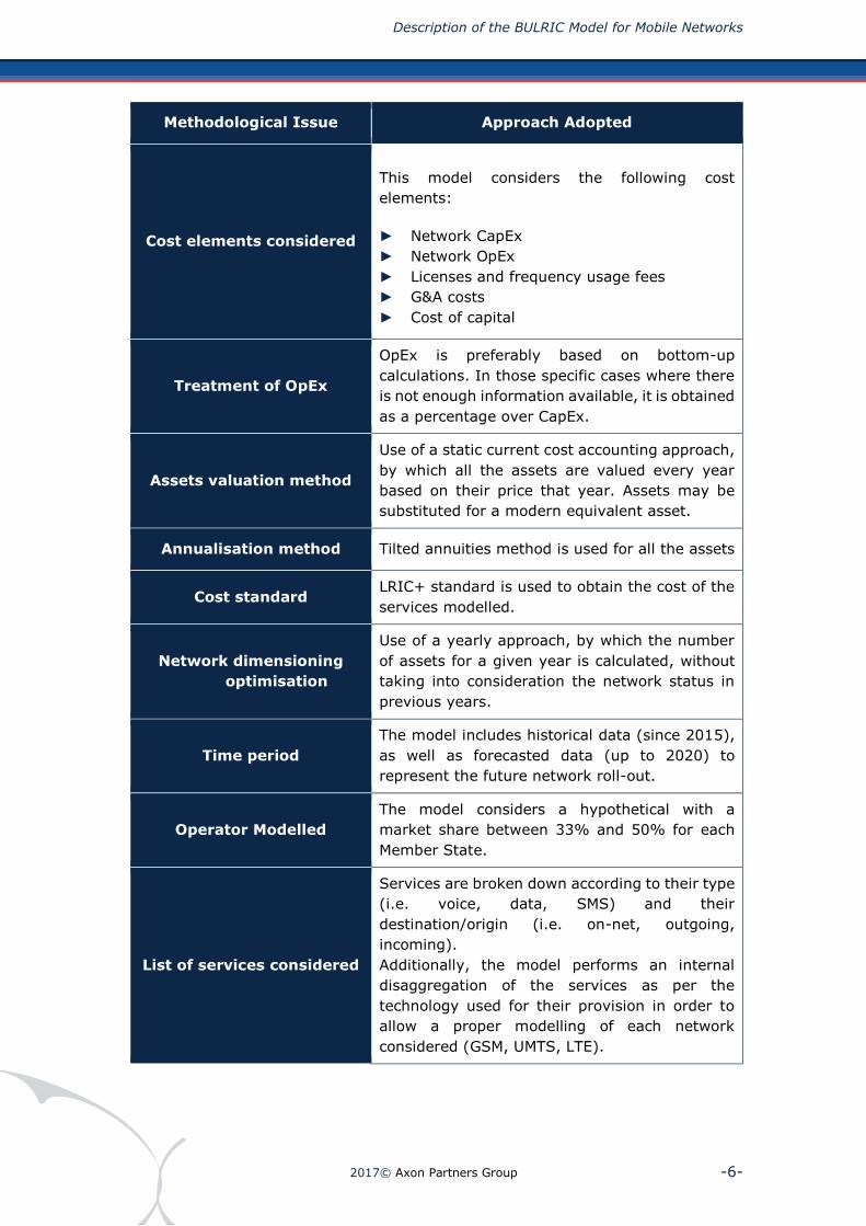
The following exhibit contains a summary of the methodological framework that has
been established to develop the model:
1 The model can be extended in future updates up to a total of 25 years 2 https://www.ectel.int/principles-methodologies-and-guidelines-for-the-determination-of-new-interconnection-rates/
Description of the BULRIC Model for Mobile Networks
2017© Axon Partners Group -6-
Methodological Issue Approach Adopted
Cost elements considered
This model considers the following cost
elements:
► Network CapEx
► Network OpEx
► Licenses and frequency usage fees
► G&A costs
► Cost of capital
Treatment of OpEx
OpEx is preferably based on bottom-up
calculations. In those specific cases where there
is not enough information available, it is obtained
as a percentage over CapEx.
Assets valuation method
Use of a static current cost accounting approach,
by which all the assets are valued every year
based on their price that year. Assets may be
substituted for a modern equivalent asset.
Annualisation method Tilted annuities method is used for all the assets
Cost standard LRIC+ standard is used to obtain the cost of the
services modelled.
Network dimensioning
optimisation
Use of a yearly approach, by which the number
of assets for a given year is calculated, without
taking into consideration the network status in
previous years.
Time period
The model includes historical data (since 2015),
as well as forecasted data (up to 2020) to
represent the future network roll-out.
Operator Modelled
The model considers a hypothetical with a
market share between 33% and 50% for each
Member State.
List of services considered
Services are broken down according to their type
(i.e. voice, data, SMS) and their
destination/origin (i.e. on-net, outgoing,
incoming).
Additionally, the model performs an internal
disaggregation of the services as per the
technology used for their provision in order to
allow a proper modelling of each network
considered (GSM, UMTS, LTE).

Description of the BULRIC Model for Mobile Networks
2017© Axon Partners Group -7-
Methodological Issue Approach Adopted
Definition of the
increments
Increments are defined based on service type,
differentiating between voice and data and other
services.
Geotypes
Geotypes are based on population centres
(considering their population, population density
and density of population centres) as well as
their orography.
Network topology
The model will use a scorched earth approach to
model the access network and a modified
scorched node approach to model the core
network.
Mobile Access
Technologies
The model uses a combination of 2G/3G/4G
technologies, according to the availability of each
for the operators.
Transmission technologies
Incorporates the following mix of technologies:
► Microwaves
► Leased lines
► Own fibre links
Core Network and
Backbone
Considers a 3Gpp legacy core network for the 2G
and 3G access technologies and an evolved core
network for the 4G access.
Exhibit 1.1: Summary of the methodological framework. [Source: Axon Consulting]
1.2. Structure of the document
The remaining sections of this document describe:
The modelling approach
The model structure
The calculation process
The document is structured as follows:
General Architecture of the Model: introduces the general structure of the model,
from the demand module to the network dimensioning and costing modules
Model : introduces the main inputs needed for the model

Description of the BULRIC Model for Mobile Networks
2017© Axon Partners Group -8-
Dimensioning Drivers: examines the conversion of traffic (at service level) to
network parameters (for example, Erlangs and Mbps) facilitating the
dimensioning of network resources
Geographical Analysis: presents the treatment performed to the geographical
area of the Sultanate in order to adapt it to the needs of the BULRIC Model
Dimensioning Module: illustrates the criteria followed in order to design the
network and calculate the number of resources required to meet coverage and
capacity constraints
Cost Calculation Module: shows expenditure calculations (CapEx and OpEx)
associated to the network resources dimensioned in the dimensioning module
Depreciation Module: presents the calculation of the depreciation method to
distribute CapEx over the years (annualisation)
Incremental Costs Calculations: includes further explanations about the
calculation of costs under LRIC+ standard
Finally, a user manual has been produced and is provided as a separate document.

Description of the BULRIC Model for Mobile Networks
2017© Axon Partners Group -9-
2. General Architecture of the Model
This chapter of the document introduces the general structure of the model. The
following figure shows the function blocks and their interrelationship within the
model.
Exhibit 2.1: Structure of the model [Source: Axon Consulting]
Several function blocks can be identified but, as a first classification, the following
parts are described below:
Dimensioning drivers: Converting traffic into dimensioning drivers, later assisting
in dimensioning network resources
Dimensioning module: Computing the number of resources and building the
network that can supply the main services provided by the reference operator. It
comprises different modules such as GSM, UMTS, LTE, sites, and backhaul,
backbone and core network
The estimated traffic for all modelled services is used by the Dimensioning Module.
Additionally, geographical data is introduced in the dimensioning module to take into
consideration the relevant geographical aspects of each Member State.
LRIC Calculation Module
FDC Cost Allocation Module
Cost Annualisation Module
Resources Costing (CAPEX & OPEX)
DIMENSIONING MODULE
Geotype Dependent Geotype Independent
RAN GSM
RAN UMTS
RAN LTE
Sites and Backhaul Dimensioning
Core Network&
Backbone
DIMENSIONING DRIVERS
Results: Network costs by service
Demand
Geo
grap
hic
al D
ata
, C
overag
e a
nd
Sp
ectr
um
Bottom-Up LRICModel architecture

Description of the BULRIC Model for Mobile Networks
2017© Axon Partners Group -10-
The model recognises that the different parts of the reference operator’s network can
be geotype-dependent or -independent. For example, the dimensioning process
corresponding to GSM, UMTS, LTE, Sites and Backhaul is distinctive and independent
for each geotype.
Dimensioning drivers: Converting traffic into dimensioning drivers, later assisting
in dimensioning network resources
Cost calculation (CapEx and OpEx): calculating cost of resources obtained after
network dimensioning, both in terms of CapEx and OpEx
Annualisation module: allocating CapEx resources costs over time following under
the methodology defined, i.e., employing a tilted annuities method.
Cost imputation to services module: calculating the costs of services by means of
resources costs imputation to different services according to a Fully Distributed
Cost (FAC) approach
Incremental costs calculation module: obtaining pure incremental costs related
to the different increments (each increment is defined as a group of services) and
common costs
The following sections further develop each block of the model:

Description of the BULRIC Model for Mobile Networks
2017© Axon Partners Group -11-
3. Model Inputs
By definition, the main input for a BU-LRIC model is the demand that should be
satisfied by the network to be dimensioned. However, additional data is required. The
following list describes the main inputs that are needed for the BULRIC Model:
Coverage: the coverage achieved (usually measured as a percentage of
population covered) has a considerable impact on the results of the model.
Therefore, historical and forecast coverage by geotype is input in the model
Spectrum: the main constraint for the development of mobile networks. It is also
important to consider the allocation of spectrum bands to technologies. This input
can vary along the time frame considered and can be different for each geotype
Geographical information: for the dimensioning of the network, certain
information about the countries needs to be considered. This information is
aggregated into geotypes with homogeneous characteristics (e.g. population
density, orography). Additionally, the characterisation of the core network is
needed (e.g. core locations, links). Geographical information is produced by using
public information (e.g. coordinates and population of the population centres)
Traffic statistics: for the dimensioning of the network it is necessary to know
certain statistics of the network (e.g. concentration of traffic in the busy hour,
average call duration)
Network dimensioning parameters and equipment capacity: dimensioning
algorithms need information about the characteristics of the equipment. A
number of them are common among manufacturers or are fixed by the technology
or the standard

Description of the BULRIC Model for Mobile Networks
2017© Axon Partners Group -12-
4. Dimensioning Drivers
The rationale of the dimensioning drivers is to express traffic and demand (at service
level) in a way that facilitates the dimensioning of network resources.
This section presents the following features of the dimensioning drivers:
Concept
Mapping services to drivers
Conversion factors from services to drivers
4.1. Dimensioning drivers concept
The recognition of dimensioning "drivers" is intended to simplify and increase the
transparency of the network dimensioning process.
Dimensioning drivers represent, among others, the following requirements:
Erlangs
UMTS bearers CS12,2 (Channel Switched 12,2Kbps is used for voice calls) and
CS64 (Channel Switched 64Kbps is used for video calls)
Mbps for packet switching carriers GPRS / EDGE / UMTS / HSPA (divided into
uplink and downlink)
Mbps for transmission through the core network
Total number of subscribers for the dimensioning of HLR
The following list contains the drivers used in the BULRIC model:
VARIABLE
DRIV.GSM.VOICE.Channels
DRIV.GSM.GPRS.Download Channels
DRIV.GSM.EDGE.Download Channels
DRIV.GSM.SIGNAL.Channels
DRIV.UMTS.CS.Voice
DRIV.UMTS.CS.VideoCalls
DRIV.UMTS.Data PS.PS64-DL
DRIV.UMTS.Data PS.PS64-UL
DRIV.UMTS.Data PS.PS128-DL
DRIV.UMTS.Data PS.PS128-UL
DRIV.UMTS.Data PS.PS384-DL

Description of the BULRIC Model for Mobile Networks
2017© Axon Partners Group -13-
VARIABLE
DRIV.UMTS.Data PS.PS384-UL
DRIV.UMTS.Data HSPA-B.HSPA-Best Effort-DL
DRIV.UMTS.Data HSPA-B.HSPA-Best Effort-UL
DRIV.UMTS.Data HSPA-QoS.HSPA-Gold-DL
DRIV.UMTS.Data HSPA-QoS.HSPA-Gold-UL
DRIV.UMTS.Data HSPA-QoS.HSPA-Real Time-DL
DRIV.UMTS.Data HSPA-QoS.HSPA-Real Time-UL
DRIV.UMTS.SIGNAL.SIGNAL
DRIV.LTE.Data LTE-B.Best Effort-DL
DRIV.LTE.Data LTE-B.Best Effort-UL
DRIV.LTE.Data LTE-QoS.Gold-DL
DRIV.LTE.Data LTE-QoS.Gold-UL
DRIV.LTE.Data LTE-QoS.Real Time-DL
DRIV.LTE.Data LTE-QoS.Real Time-UL
DRIV.LTE.SIGNAL.SIGNAL
DRIV.BACKHAUL 2G.VOICE.GSM
DRIV.BACKHAUL 2G.DATA.GPRS/EDGE
DRIV.BACKHAUL 2G.SMS-MMS.GSM
DRIV.BACKHAUL 3G.VOICE.UMTS
DRIV.BACKHAUL 3G.VIDEOCALL.UMTS
DRIV.BACKHAUL 3G.DATA.UMTS/HSPA Best Effort
DRIV.BACKHAUL 3G.DATA.HSPA Gold
DRIV.BACKHAUL 3G.DATA.HSPA Real Time
DRIV.BACKHAUL 3G.DATA.UMTS SMS-MMS
DRIV.BACKHAUL 4G.DATA.LTE Best Effort
DRIV.BACKHAUL 4G.DATA.LTE Gold
DRIV.BACKHAUL 4G.DATA.LTE Real Time
DRIV.BACKHAUL 2G.SIGNAL.GSM
DRIV.BACKHAUL 3G.SIGNAL.UMTS
DRIV.BACKHAUL 4G.SIGNAL.LTE
DRIV.CORE NGN 2G.BHCA.2G
DRIV.CORE NGN 3G.BHCA.3G
DRIV.CORE NGN 4G.BHCA.4G
DRIV.CORE CS_PS.TRAFFIC.CORE VOICE/VIDEO/SMS/MMS
DRIV.CORE CS_PS.TRAFFIC.CORE DATA
DRIV.CORE 2G TRAFFIC.TRAFFIC.CORE 2G TRAFFIC
DRIV.CORE 2G TRAFFIC.SIGNAL.CORE 2G TRAFFIC
DRIV.CORE 3G TRAFFIC.TRAFFIC.CORE 3G TRAFFIC
DRIV.CORE 3G TRAFFIC.SIGNAL.CORE 3G TRAFFIC
DRIV.CORE 4G TRAFFIC.TRAFFIC.CORE 4G TRAFFIC
DRIV.CORE 4G TRAFFIC.SIGNAL.CORE 4G TRAFFIC
DRIV.CORE DATA TRAFFIC.TRAFFIC.CORE 2G DATA TRAFFIC
DRIV.CORE DATA TRAFFIC.SIGNAL.CORE 2G DATA TRAFFIC
DRIV.CORE DATA TRAFFIC.TRAFFIC.CORE 3G DATA TRAFFIC
DRIV.CORE DATA TRAFFIC.SIGNAL.CORE 3G DATA TRAFFIC
DRIV.CORE.TRAFFIC.CORE 4G DATA TRAFFIC

Description of the BULRIC Model for Mobile Networks
2017© Axon Partners Group -14-
VARIABLE
DRIV.CORE.SIGNAL.CORE 4G DATA TRAFFIC
DRIV.CORE SMS.TRAFFIC.SMS 2G
DRIV.CORE SMS.TRAFFIC.SMS 3G
DRIV.CORE SMS.TRAFFIC.SMS 4G
DRIV.CORE MMS.TRAFFIC.MMS 2G
DRIV.CORE MMS.TRAFFIC.MMS 3G
DRIV.CORE MMS.TRAFFIC.MMS 4G
DRIV.CORE.TRAFFIC.BHCA 2G
DRIV.CORE.TRAFFIC.BHCA 3G
DRIV.CORE.TRAFFIC.BHCA 4G
DRIV.CORE 2G SUBS.TOTAL SUBSCRIBERS.TOTAL 2G SUBSCRIBERS
DRIV.CORE 3G SUBS.TOTAL SUBSCRIBERS.TOTAL 3G SUBSCRIBERS
DRIV.CORE 4G SUBS.TOTAL SUBSCRIBERS.TOTAL 4G SUBSCRIBERS
DRIV.CORE 2G SUBS MNO.TOTAL SUBSCRIBERS.TOTAL MNO 2G SUBSCRIBERS
DRIV.CORE 3G SUBS MNO.TOTAL SUBSCRIBERS.TOTAL MNO 3G SUBSCRIBERS
DRIV.CORE 4G SUBS MNO.TOTAL SUBSCRIBERS.TOTAL MNO 4G SUBSCRIBERS
DRIV.CORE 2G SUBS SAU.SUBSCRIBERS.SAU 2G
DRIV.CORE 3G SUBS SAU.SUBSCRIBERS.SAU 3G
DRIV.CORE 4G SUBS SAU.SUBSCRIBERS.SAU 4G
DRIV.CORE DATA SAU SUBS.SUBSCRIBERS.DATA SAU 2G
DRIV.CORE DATA SAU SUBS.SUBSCRIBERS.DATA SAU 3G
DRIV.CORE.SUBSCRIBERS.DATA SAU 4G
DRIV.CORE IX.TRAFFIC.IX CS
DRIV.CORE II.TRAFFIC.IX DATA
DRIV.CORE IX.SIGNAL.IX CS
DRIV.CORE II.SIGNAL.IX DATA
DRIV.CORE 2G MULT IX.TRAFFIC.Multimedia IX 2G
DRIV.CORE 3G MULT IX.TRAFFIC.Multimedia IX 3G
DRIV.CORE 4G MULT IX.TRAFFIC.Multimedia IX 4G
DRIV.CORE ERLANGS.TRAFFIC.CS 2G-3G
DRIV.CORE BILLING.BILLING.EVENTS 2G
DRIV.CORE BILLING.BILLING.EVENTS 3G
DRIV.CORE BILLING.BILLING.EVENTS 4G
Exhibit 4.1: List of Drivers used in the model (Sheet ‘0D PAR DRIVERS’). [Source: Axon
Consulting]
Two steps are required to calculate the drivers:
1. Mapping services to drivers
2. Converting traffic units into the corresponding driver units
These steps are discussed below in more detail.

Description of the BULRIC Model for Mobile Networks
2017© Axon Partners Group -15-
4.2. Mapping internal services to drivers
To obtain drivers it is necessary to indicate which services are related to them. It
should be noted that a service is generally assigned to more than one driver, as
drivers represent traffic in a particular point of the network.
This operation is performed at the internal service level, with information regarding
the technological disaggregation. These services are only defined internally in the
model as a disaggregation of the so-called ‘external services’ (the services whose
cost is ultimately calculated in the model that do not differentiate between
technology). This disaggregation is based on the data regarding the split of traffic
among technologies provided by operators.
For example, voice calls on net should be contained in both the drivers used to
dimension radio access and those used for the core network.
The following exhibit shows an excerpt of the mapping of services into drivers:
List of relationships
SERVICE (Variable Name) DRIVER (Variable Name)
UMTS.Voice.On-net.Retail.On-net DRIV.UMTS.CS.Voice
UMTS.Voice.On-net.Retail.On-net to voicemail DRIV.UMTS.CS.Voice
UMTS.Voice.On-net.Retail.On-net to directory assistance DRIV.UMTS.CS.Voice
UMTS.Voice.On-net.Retail.On-net to customer services DRIV.UMTS.CS.Voice
UMTS.Voice.On-net.Retail.On-net to emergency services DRIV.UMTS.CS.Voice
UMTS.Voice.Outgoing.Retail.Off-net to other mobile DRIV.UMTS.CS.Voice
UMTS.Voice.Outgoing.Retail.Off-net to fixed DRIV.UMTS.CS.Voice
UMTS.Voice.Outgoing.Retail.Off-net to international DRIV.UMTS.CS.Voice
UMTS.Voice.Outgoing.Wholesale.MVNO - Origination DRIV.UMTS.CS.Voice
UMTS.Voice.Incoming.Wholesale.MVNO - Termination DRIV.UMTS.CS.Voice
UMTS.Voice.Incoming.Wholesale.Incoming from national DRIV.UMTS.CS.Voice
UMTS.Voice.Incoming.Wholesale.Incoming from international DRIV.UMTS.CS.Voice
Exhibit 4.2: Except from the Mapping of Services into Drivers. (Sheet ‘3B MAP SERV2DRIV’)
[source: Axon Consulting]
4.3. Conversion factors from services to drivers
Once services have been mapped to drivers, volumes need to be converted to obtain
drivers in proper units.
For that purpose, a conversion factor that represents the number of driver units
generated by each demand service unit has been developed. In general, the
Description of the BULRIC Model for Mobile Networks
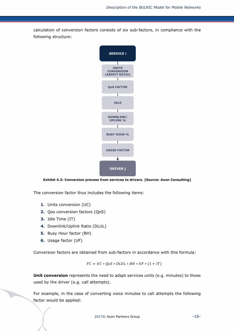
2017© Axon Partners Group -16-
calculation of conversion factors consists of six sub-factors, in compliance with the
following structure:
Exhibit 4.3: Conversion process from services to drivers. [Source: Axon Consulting]
The conversion factor thus includes the following items:
1. Units conversion (UC)
2. Qos conversion factors (QoS)
3. Idle Time (IT)
4. Downlink/Uplink Ratio (DLUL)
5. Busy Hour factor (BH)
6. Usage factor (UF)
Conversion factors are obtained from sub-factors in accordance with this formula:
𝐹𝐶 = 𝑈𝐶 ∗ 𝑄𝑜𝑆 ∗ 𝐷𝐿𝑈𝐿 ∗ 𝐵𝐻 ∗ 𝑈𝐹 ∗ (1 + 𝐼𝑇)
Unit conversion represents the need to adapt services units (e.g. minutes) to those
used by the driver (e.g. call attempts).
For example, in the case of converting voice minutes to call attempts the following
factor would be applied:
SERVICE i
DRIVER j
UNITS CONVERSION
(ASPECT RATIO)
QoS FACTOR
IDLE
DOWNLINK/UPLINK %
USAGE FACTOR
BUSY HOUR %

Description of the BULRIC Model for Mobile Networks
2017© Axon Partners Group -17-
𝑈𝐶 =1 + 𝑃𝑁𝑅 + 𝑃𝑁𝐴
𝑇𝑀
Where PNR is the percentage of non-attended calls, PNA is the percentage where the
recipient is not available (device off, out of coverage, etc.), and TM is the average
call time in minutes.
The quality of service represents the dimensioning factor required to meet all QoS
goals in the busy hour.
For circuit-switched and packet-switched services with QoS, it is necessary to apply
Erlang tables to reach the adequate dimensioning for a given blocking probability3.
Idle time represents the difference between the conveyed traffic from the users’
viewpoint and the required resource consumption the network needs to face.
For the calculation of idle-time factor the following aspects have been taken into
account:
Time required to set up the connection, which is not considered as time of service.
It represents waiting time until the recipient picks up the phone to accept the
call. During that time an actual resources assignation is produced. For the
calculation of the factor this formula is used:
𝐶𝑜𝑛𝑛𝑒𝑐𝑡𝑖𝑜𝑛 𝑇𝑖𝑚𝑒 𝑃𝑒𝑟𝑐𝑒𝑛𝑡𝑎𝑔𝑒 = 𝐴𝑅𝑇/𝐴𝐶𝐷
Where ART it is the average ringing time and ACD the average duration time of
the call.
Missed calls: Non-attended calls, for general recipient unavailability.
This factor even takes into consideration communications to notify the
impossibility of completing the call.
This is the formula used:
% 𝑜𝑓 𝑛𝑜𝑡 𝑎𝑡𝑡𝑒𝑛𝑑𝑒𝑑 𝑐𝑎𝑙𝑙𝑠 =
𝑃𝑁𝑅𝐶
1−𝑃𝑁𝑅𝐶−𝑃𝑂∗ 𝐴𝑅𝑇 +
𝑃𝑂
1−𝑃𝑁𝑅𝐶−𝑃𝑂∗ 𝐴𝑇
𝐴𝐶𝐷
Where PNRC represents the percentage of non answered calls, PO is the
percentage of calls where the recipient is busy, ART is the average ringing time
and AT is the duration time of the message indicating the failure to establish the
call.
3 For the access drivers, QoS is directly considered during the dimensioning process, making direct use of Erlang tables.

Description of the BULRIC Model for Mobile Networks
2017© Axon Partners Group -18-
Inefficiencies in resource usage: this factor, which is very common in data
communications, represents the time a user is assigned a channel even if it is
neither receiving, nor transmitting data (due to burstiness of data traffic).
Although the technologies under consideration have systems for resources
reassignment, a share of network capacity will be lost. This inefficiency factor is
highly dependent on the technology used and the features of the typology of data
traffic. To obtain the parameter the following formula is employed:
% of employed traffic = Bmax ∗(ts + tc)
𝐵𝑎𝑣 ∗ 𝑡𝑠− 1
Where Bmax it is the maximum bit rate assigned to the user, ts the average time
of assigned slot, tc the resources reconfiguration time and Bav the average bit
rate employed by the user. These parameters may vary in relation to the
technologies used.
The downlink/uplink ratio applies to data transmission services and represents
the percentage of the service’s total traffic carried in each direction, that is, the
percentage of data sent or received by the user.
It should be pointed out, that, for dimensioning purposes, it is necessary to know the
amount of data transmitted in one direction (the more dominant for GSM) or in both
(for UMTS dimensioning is done separately to satisfy both uplink and downlink
demand).
Busy hour factor represents the percentage of traffic that is carried in one busy hour
over the total yearly traffic.
Usage factor represents the number of times a service makes use of a specific
resource. For example, when obtaining drivers used for access network dimensioning,
it is necessary to ensure that on-net services will use two radio accesses (one for the
caller and one for the receiver). On the contrary, off-net and termination services will
use just one radio access.
However, when obtaining drivers for core dimensioning, it is necessary to consider
that, for example, not all GSM calls will make use of MSC-MSC transmission, since a
percentage will be made within the same MSC and therefore won’t be passed on
through main core rings.
Usage factor then reflects the average effect of “routing” of different services through
network topology.

Description of the BULRIC Model for Mobile Networks
2017© Axon Partners Group -19-
5. Geographical Analysis
5.1. Introduction
The design of mobile access networks is highly dependent on the geographical
characteristics of the zone to be covered, as well as on the demand.
The main purpose of this analysis is to aggregate the areas with similar characteristics
(e.g. population density, orography) into geotypes. Geotypes will be used for the
dimensioning of access and backhaul networks, which is detailed in section 6.
As defined in the methodology, the modelling approach depends on the network
segment as follows:
Access network: based on a scorched earth approach. This requires an analysis
of the population centres in order to model a network from scratch.
Core network: based on a scorched node approach. In this case, an understanding
the networks deployed by the operators is necessary.
5.2. Geographical analysis for access network
The steps below have been followed in the geographical analysis for the access
network (including radio access nodes and backhaul transmission):
1. Break down of the country into samples
2. Assignment of population centres to samples
3. Orography recognition
4. Aggregation of samples into geotypes, considering roads as a sample-
independent geotype
These steps followed for each Member State.
5.2.1. Break down the country into samples
The first step consists of the division of the total area of the country into samples.
Each sample represents a square containing a number of population centres (e.g.
cities, villages).
The following exhibit shows an example of the grid used for breaking down the
member states into samples (each small square is a sample):

Description of the BULRIC Model for Mobile Networks
2017© Axon Partners Group -20-
Exhibit 5.1: Illustrative example of grid applied to an area of a member state. [Source: Axon
Consulting]
5.2.2. Assigning population centres to samples
Once the grid is defined, the population centres4 are assigned to the sample in which
they are located. The following exhibit illustrates the process of allocation:
Exhibit 5.2: Illustrative example of aggregation of population centres (yellow circles) into
samples (blue square) [Source: Axon Consulting]
This process has been followed for all the population centres existing in the countries
analysed.
4 Population centre names, coordinates and population have been extracted from www.geonames.org

Description of the BULRIC Model for Mobile Networks
2017© Axon Partners Group -21-
The result of this step is the number of population centres and the population
contained in each sample. This information will be used later on to define the
geotypes.
5.2.3. Orography recognition
The orography is one of the most limiting geographical characteristics of mobile
networks. It is relevant because it has a direct effect on the area covered by one
base station and, therefore, to the number of sites needed. For instance, radio
coverage is lower in highly mountainous areas than in flat ones.
For the recognition of the orography characteristics of the samples, several measures
of elevation have been made in different points of each sample.
The following figures provide an example of the orography measurement followed.
Exhibit 5.3: Illustrative example of orography measurement process [Source: Axon
Consulting]
Once the measures are obtained, the difference between the highest and lowest
elevation points surrounding the population centres will represent its orography (the
higher the difference, the more mountainous the sample). The difference is called
“delta”.
Description of the BULRIC Model for Mobile Networks
2017© Axon Partners Group -22-
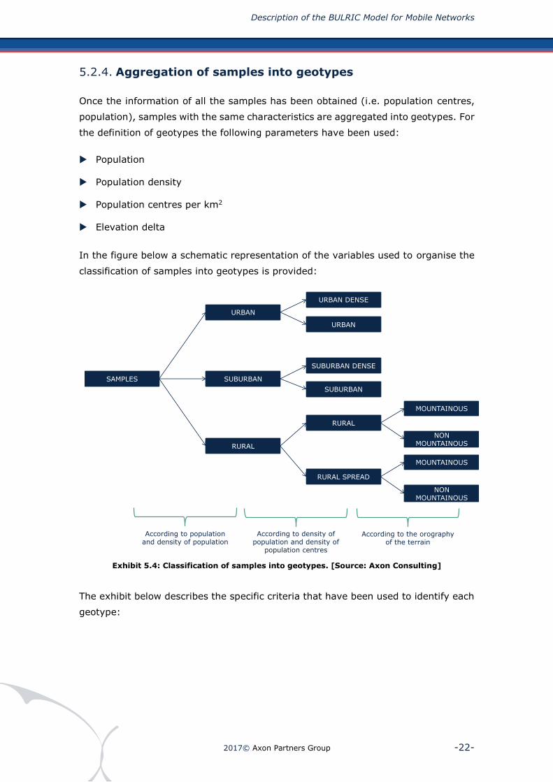
5.2.4. Aggregation of samples into geotypes
Once the information of all the samples has been obtained (i.e. population centres,
population), samples with the same characteristics are aggregated into geotypes. For
the definition of geotypes the following parameters have been used:
Population
Population density
Population centres per km2
Elevation delta
In the figure below a schematic representation of the variables used to organise the
classification of samples into geotypes is provided:
Exhibit 5.4: Classification of samples into geotypes. [Source: Axon Consulting]
The exhibit below describes the specific criteria that have been used to identify each
geotype:
SAMPLES
URBAN
SUBURBAN
RURAL
URBAN DENSE
URBAN
SUBURBAN DENSE
SUBURBAN
RURAL
RURAL SPREAD
According to population and density of population
According to density of population and density of
population centres
MOUNTAINOUS
NON MOUNTAINOUS
MOUNTAINOUS
NON MOUNTAINOUS
According to the orography of the terrain
ROADS

Description of the BULRIC Model for Mobile Networks
2017© Axon Partners Group -23-
GEOTYPE Description
URBAN_DENSE
Samples with a population higher than 3000 Inhab
and a density of population higher than 900
Inhab/km2
URBAN
Samples with either a population higher than 3000
Inhab or a density of population ranging from 750
to 900 Inhab/km2
SUBURBAN_DENSE
This geotype contains samples with a population
between 1500 and 3000 and a population density
higher than 600 Inhab/km2
SUBURBAN
This geotype contains samples with a population
between 1500 and 3000 and a population density
from 375 to 600 Inhab/km2
RURAL-NON
MOUNTAINOUS
Samples with more than 0.3 pop centres per km2,
with less than 1500 Inhab and with an elevation
delta of less than 100 metres
RURAL-
MOUNTAINOUS
Samples with more than 0.3 pop centres per km2,
with less than 1500 Inhab and with an elevation
delta of more than 100 metres
RURAL_SPREAD-
NON MOUNTAINOUS
Samples with less than 0.3 pop centres per km2,
with less than 1500 Inhab and with an elevation
delta of less than 100 metres
RURAL_SPREAD-
MOUNTAINOUS
Samples with less than 0.3 pop centres per km2,
with less than 1500 Inhab and with an elevation
delta of more than 100 metres
Exhibit 5.5: Description of the geotypes identified [Source: Axon Consulting]
After taking these considerations into account, the population centres of all the
countries have been aggregated into geotypes; see Annex A.

Description of the BULRIC Model for Mobile Networks
2017© Axon Partners Group -24-
5.3. Geographical analysis for core network
The analysis geographical analysis for the core network involves defining where core
nodes are located, where traffic is aggregated and the characteristics of the links that
make up the backbone.
In order to do so, we have analysed the information provided by the operators to
define the core and backbone networks that would be installed by the reference
operator. The core network defined for each member state is summarised in Annex
A.

Description of the BULRIC Model for Mobile Networks
2017© Axon Partners Group -25-
6. Dimensioning Module
The dimensioning module aims to design the network and dimension the network
resources required to serve the reference operator’s traffic. This section presents this
module’s characteristics:
Considerations on network node configuration
Considerations on spectrum
Radio access dimensioning GSM/GPRS/EDGE
Radio access dimensioning UMTS/HSPA
Radio access dimensioning LTE
Radio site dimensioning
Backhaul network dimensioning
Core network dimensioning
6.1. Considerations on network nodes configuration
From a general point of view, a mobile network can be seen as a combination of:
A set of nodes of different type and functionalities
A set of links connecting them
The exercise of network configuration design entails a decision on the dimensioning
algorithms. As stated in the methodology, a scorched earth approach was selected
as the methodology in order to dimension the access network of the reference
operator and a modified scorched node approach was selected to model the core
network. The use of this method is defined below for both access and core networks:
Access network: The implementation of a scorched earth approach for the access
network comprises the steps described below:
1. The model will estimate the number of radio sites required per technology
and geotype to meet the coverage target.
2. The model will calculate the radio equipment required per technology and
geotype, to meet capacity requirements.
Core network: in this case, the position is more relevant (especially for the
dimensioning of the backbone links) and may depend on political, economic,

Description of the BULRIC Model for Mobile Networks
2017© Axon Partners Group -26-
demographic and geographic issues. Therefore, the number and location of the
core nodes will be based on the operators’ existing nodes.
6.2. Considerations on spectrum
An important feature of the model is the configuration of the available spectrum for
radio access networks. The amount of available spectrum (bandwidth in MHz) for the
reference operator and the portion assigned to each different technology is composed
of a series of entry values for each available band, technology and geotype.
The following parameters need to be taken into account when introducing available
spectrum in the model: technology modularity and minimum band required for each
technology.
Modularity: An integer number of spectrum modules need to be assigned to each
technology. In practice, available modules are:
❖ GSM: 0,2 MHz
❖ UMTS: 5 MHz
❖ LTE allows several bands: 1,4, 3, 5, 10, 15 and 20 MHz
Minimum bandwidth: This represents the minimum spectrum required to build a
coverage network. In case of UMTS, the minimum spectrum is equal to the
minimum module (5 MHz). Nevertheless, for GSM the frequency reuse factor also
needs to be considered (commonly 12 if using tri-sectorial cells). Therefore, for
GSM the minimum spectrum that can be assigned is 12*0.2 MHz = 2.4 MHz.
6.3. Radio access dimensioning GSM/GPRS/EDGE
6.3.1. Presentation of the algorithm for radio network
dimensioning GSM/GPRS/EDGE
The dimensioning algorithm for GSM (including GPRS and EDGE) is organised into six
steps, as shown in the chart below. Like in other dimensioning modules, this
algorithm runs separately for each of the geotypes considered.

Description of the BULRIC Model for Mobile Networks
2017© Axon Partners Group -27-
Exhibit 6.1: Steps for Radio Dimensioning GSM / GPRS / EDGE. [Source: Axon Consulting]
The dimensioning algorithm for GSM radio access network is implemented in the ‘6A
CALC DIM GSM’ sheet of the model. Each step is explained in further detail in the
following subsections.
6.3.2. Step 0. Calculation of adjusted traffic (planning horizon
and network efficiency factor)
A preliminary step to dimensioning GSM/GPRS/EDGE networks is the calculation of
traffic to be used in the traffic dependent part of the network. In the calculation of
this traffic, denominated “adjusted traffic”, two factors are involved:
1. The effect of the planning horizon: when the network is being designed, forecast
demand is taken into account to avoid necessary upgrades in the short term.
2. The overcapacity needed for security reasons.
The GSM radio network dimensioning based on traffic is done using the drivers listed
below:
DRIV.GSM.VOICE.Channels
DRIV.GSM.GPRS.Download Channels
DRIV.GSM.EDGE.Download Channels
DRIV.GSM.SIGNAL.Channels
Step 0. GSM/GPRS/EDGE Adjusted Traffic Calculation (Planning Horizon and Efficiency
Factor)
Step 2. Number of sites required for Traffic Calculation (for each type of site)
Step 1. Number of GSM Sites needed for Coverage Calculation
Step 3. GSM Sites Number Calculation (maximum among traffic or coverage) and
selection of the optimal configuration
Step 4. Number of Macro GSM Network Elements Calculation (BTS,Sectors,TRX)
Step 5. Number of GSM Micro Network Elements Calculation

Description of the BULRIC Model for Mobile Networks
2017© Axon Partners Group -28-
Drivers are broken down by voice, signalling and data, distinguishing between GPRS
and EDGE. All drivers are measured in dimensioning channels.
These drivers are calculated based on traffic demand. Please note the following:
As it has been stated previously, for mapping voice traffic on Erlangs, a
percentage of "idle" or inactive traffic was added to represent unbilled time, but
during which the network is used (e.g. time until the recipient picks up the phone,
calls not answered). A factor is applied to this "increased” traffic to calculate the
number of channels required (according to the Erlang B formula) for a given
blocking probability.
Regarding data services, an "idle" occupancy rate of the channel is taken into
consideration to model the time during which the user is assigned a channel but
is neither transmitting nor receiving any data. The system has automatic
mechanisms to detect and remove resources when not in use, but this is not an
instantaneous process. Therefore, this parameter reflects the delay between the
moment the user stops sending or receiving data and the moment the system
reallocates the unoccupied resources.
Signalling drivers are those that consider the time required for transmission of
SMS (and requests for using the channel), transmissions to coordinate call
establishment, frames for periodic location update and handover processes
depending on the number of active users.
For all drivers outlined above, the busy hour percentage and the factor of use of radio
access service apply depending on whether the services are on-net (using the radio
network at both ends of the communication) or off-net (using a single communication
endpoint).
6.3.3. Step 1. Calculation of number of sites required for
coverage
The calculation of equipment requirements for coverage is worked out for each
geotype.
The model is able to calculate the minimum number of sites required for coverage
for both GSM 700-900MHz and 1800-2600MHz bands.
The site coverage radius is adjusted depending on geotype class by defining a
percentage over the maximum radius, which is a function of the propagation
conditions for each class of geotype.

Description of the BULRIC Model for Mobile Networks
2017© Axon Partners Group -29-
The diagram below illustrates the calculation of the minimum number of sites
associated with GSM coverage.
Exhibit 6.2: Algorithm for calculating number of sites for GSM coverage (step 1). [Source:
Axon Consulting]
The maximum coverage area per cell is calculated according to the formula:
2Re2
33torductionFacRadiusMaxRadiuslAreaMaximumCel
Where MaxRadius represents the maximum coverage radius (different for GSM700-
900 and GSM1800-2600), RadiusReductionFactor is a reduction factor of the
maximum coverage radius depending on geotype, and the constant factor
corresponds to the area of a hexagon.
The number of required sites to cover the geotype in a band is obtained by dividing
the area to be covered by the Area per site (Maximum Cell Area multiplied by the
number of sectors).
Additionally, it is common in spread areas to deploy the coverage based on the
population centres. That is, cells are not intended to cover all the area but only the
populated centres. This option can be selected by geotype, being the default option
to be applied only in rural geotypes.
Maximum theoretical coverage area per cell
GSM900 GSM1800
Outputs
Calculations
Inputs
Geotype AreaNumber of Population
Centers
Sites Needed GSM1800 = Area to be covered / Maximum Area per Cell
GSM 1800 / Sectors per Site(Spectrum availability is checked)
Minimum sites for Coverage
GSM900/GSM1800
Sites Needed GSM900 = Area to be covered / Maximum Area per Cell
GSM 900 / Sectors per Site(Spectrum availability is checked)
Area to be covered=
Area x
% GSM Coverage
Sites Needed=
Population Centers
(specially in rural areas)
% Covered Area Adjustment by
Geotype
Calculation of
Maximum Area of a Cell
GSM900/GSM1800
Number of Sectors per Site (GeotypeDependent)
Centers to be covered= Centers
x % GSM Coverage

Description of the BULRIC Model for Mobile Networks
2017© Axon Partners Group -30-
6.3.4. Step 2. Calculating the number of GSM sites for macro
cells required in terms of traffic
The third step is to determine the number of necessary sites to serve voice and data
traffic demand as well as associated signalling requirements. The diagram below
shows the dimensioning algorithm used for this purpose.
Please note this algorithm is used for different potential configurations of the sites,
depending on the number of sectors (2 or 3) and spectrum bands used. The two
sector cells are applicable only for roads or railways geotypes.
Exhibit 6.3: Algorithm for calculating the number of sites for GSM traffic (step 2). [Source:
Axon Consulting]
The following aspects are of interest in relation to the algorithm for calculating the
number of GSM sites based on traffic:
The total traffic in the dominant busy hour is multiplied by a factor (1 -% micro)
to eliminate the percentage of traffic served by micro cells. This percentage
depends on the geotype
GPRS/EDGE Adjusted Downlink Data Traffic
(Channels)
GSM Adjusted Voice Traffic (Channels)
Available Spectrum 900MHz , 1800MHz(incl. RAN sharing
effect)
MAXIMUM
Adjusted Downstream Signaling Traffic
(Channels)
Available Channels= Available Spectrum /
Channel Bandwidth (0,2 MHz)
Maximum Channels per Cell=
Available Channels / Reuse Factor
Voice Traff. Macro + BH Data=
Voice Traff. Macro + BH Data x (1-%micro-pico)
BH Signaling Traff. Macro=
BH Signaling Traff.x (1 - %micro-pico)
Number of Sites required for traffic
(assuming minimum signaling channels per cell)
Sites =
(Voice Traff. + BH Data) /
(Max. Channels per Cell –min signalling channels)
/ Sectors per Site
Number of Sites required for traffic
(assuming signaling traffic dominant)
Sites =
(Voice Traff. + BH Data + Signaling) /
(Max. Channels per Cell) /
Sectors per Site
Number of sites required by Traffic
Outputs
Calculations
Inputs

Description of the BULRIC Model for Mobile Networks
2017© Axon Partners Group -31-
The available spectrum has a direct impact on the number of sites, since it
determines the maximum number of channels per cell
The frequency reuse factor depends on the number of sectors per site and the
use of micro equipment in the geotype. Using the parameter of the number of
TRX by micro equipment, the frequency reuse factor will increase in proportion to
ensure there are always available frequencies for micro equipment in geotypes
where they exist
The estimation of the number of sites takes into account the need of at least two
channels per cell dedicated to signalling
Using these rules the following parameters are obtained:
K: the number of base stations needed to meet demand when employing only
band 1 (700-900MHz)
L: the number of base stations needed to meet demand when employing only
band 2 (1800-2600MHz).
6.3.5. Step 3. Calculating the optimal configuration and number
of sites
Step 3 of the dimensioning algorithm determines the number of macro sites required
for each possible configuration of the site, taking into account coverage and capacity
constraints. Based on this result, the optimal configuration is defined as that which
minimises the number of required sites, as it is assumed that the costs associated
with construction and maintenance of the site are the most significant. Given the
adoption of a yearly approach for determining the configuration of the network, this
process is totally independent of the network status in previous years.
6.3.6. Step 4. Calculating the number of macro network
elements
Once the number of sites required and the corresponding configuration has been
identified, step 4 proceeds to calculate the number of required macro network
elements. These include the number of base stations (which can support both 700-
Description of the BULRIC Model for Mobile Networks
2017© Axon Partners Group -32-
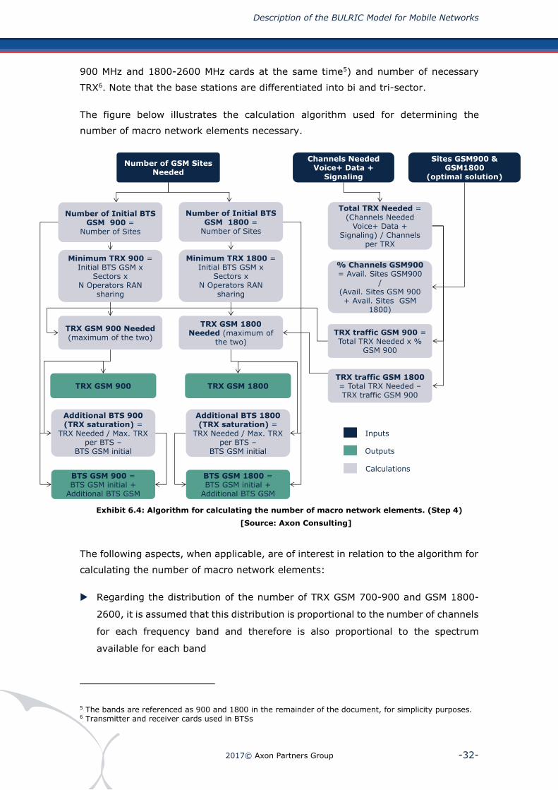
900 MHz and 1800-2600 MHz cards at the same time5) and number of necessary
TRX6. Note that the base stations are differentiated into bi and tri-sector.
The figure below illustrates the calculation algorithm used for determining the
number of macro network elements necessary.
Exhibit 6.4: Algorithm for calculating the number of macro network elements. (Step 4)
[Source: Axon Consulting]
The following aspects, when applicable, are of interest in relation to the algorithm for
calculating the number of macro network elements:
Regarding the distribution of the number of TRX GSM 700-900 and GSM 1800-
2600, it is assumed that this distribution is proportional to the number of channels
for each frequency band and therefore is also proportional to the spectrum
available for each band
5 The bands are referenced as 900 and 1800 in the remainder of the document, for simplicity purposes. 6 Transmitter and receiver cards used in BTSs
BTS GSM 900 = BTS GSM initial +
Additional BTS GSM
Channels Needed Voice+ Data +
Signaling
Number of GSM Sites Needed
Additional BTS 900 (TRX saturation) =
TRX Needed / Max. TRX per BTS –
BTS GSM initial
TRX GSM 900 TRX GSM 1800
Sites GSM900 & GSM1800
(optimal solution)
BTS GSM 1800 = BTS GSM initial +
Additional BTS GSM
Outputs
Calculations
Inputs
Minimum TRX 900 = Initial BTS GSM x
Sectors x N Operators RAN
sharing
TRX traffic GSM 900 = Total TRX Needed x %
GSM 900
Total TRX Needed = (Channels Needed
Voice+ Data + Signaling) / Channels
per TRX
Number of Initial BTS GSM 900 =
Number of Sites
Minimum TRX 1800 = Initial BTS GSM x
Sectors x N Operators RAN
sharing
% Channels GSM900 = Avail. Sites GSM900
/ (Avail. Sites GSM 900 + Avail. Sites GSM
1800)
TRX GSM 900 Needed (maximum of the two)
TRX traffic GSM 1800 = Total TRX Needed –TRX traffic GSM 900
TRX GSM 1800 Needed (maximum of
the two)
Number of Initial BTS GSM 1800 =
Number of Sites
Additional BTS 1800 (TRX saturation) =
TRX Needed / Max. TRX per BTS –
BTS GSM initial

Description of the BULRIC Model for Mobile Networks
2017© Axon Partners Group -33-
The algorithm takes into account that each location must have at least one base
station. Also, at least one TRX per sector is required
If the number of TRX per base stations exceeds the limit that supports the base
station (technical limitations), it is assumed that new BTS equipment will need to
be installed in order to accommodate additional TRX. These BTS in the chart
above are called "extra” base stations
6.4. Radio access dimensioning UMTS/HSPA
6.4.1. Presentation of the dimensioning algorithm for radio
network UMTS/HSPA
The dimensioning algorithm for UMTS (including HSPA) is organised into nine steps,
as shown in the chart below.
Like the other dimensioning modules, this algorithm runs separately for each geotype
considered. Unlike in GSM radio dimensioning, for UMTS it is necessary to perform
the dimensioning separately for the uplink and downlink to determine which one is
dominant.

Description of the BULRIC Model for Mobile Networks
2017© Axon Partners Group -34-
Exhibit 6.5: Steps for radio dimensioning UMTS/HSPA. [Source: Axon Consulting]
The dimensioning algorithm of the UMTS radio access network is implemented in the
‘6B CALC DIM UMTS’ of the model. Each step is described in further detail in the
following sections.
6.4.2. Step 0. Adjusted traffic calculation (planning horizon and
efficiency factor)
A preliminary step to dimensioning a UMTS/HSPA network is the calculation of the
traffic. In the calculation of this traffic, denominated "adjusted traffic”, two factors
are involved:
1. The effect of the planning horizon
2. Overcapacity for security reasons
The UMTS/HSPA radio network dimensioning in terms of traffic is carried out from
the drivers listed below:
Step 0. Adjusted Traffic Calculation(Planning Horizon and Overcapacity)
Step 2. HSPA Bandwidth needed by QoSCalculation (Real Time, Gold, Best Effort)
Step 1. Number of sites required for Coverage Calculation
Step 5. Determination of the Number of Sites and Carriers
Step 7. Calculation of the Number of UMTS Macro Network Elements (Node B, Sectors,
Carriers)
Step 9. Calculation of the Number of Micro/Pico
Network Elements
Step 4. Calculation of Normalized Traffic on voice channels for UMTS + HSPA
Step 6. Number of Sites Calculation (maximum DL or UL) and selection of the
Optimal Configuration
Step 8. Calculation of the Number of HSPA Macro Network Elements (SW Releases)
Step 3. Determination of the appropriate HSPA Release
SeparatedDimensioning forDownlink / Uplink
Description of the BULRIC Model for Mobile Networks
2017© Axon Partners Group -35-
DRIV.UMTS.CS.Voice
DRIV.UMTS.CS.VideoCalls
DRIV.UMTS.Data PS.PS64-DL
DRIV.UMTS.Data PS.PS64-UL
DRIV.UMTS.Data PS.PS128-DL
DRIV.UMTS.Data PS.PS128-UL
DRIV.UMTS.Data PS.PS384-DL
DRIV.UMTS.Data PS.PS384-UL
DRIV.UMTS.Data HSPA-B.HSPA-Best Effort-DL
DRIV.UMTS.Data HSPA-B.HSPA-Best Effort-UL
DRIV.UMTS.Data HSPA-QoS.HSPA-Gold-DL
DRIV.UMTS.Data HSPA-QoS.HSPA-Gold-UL
DRIV.UMTS.Data HSPA-QoS.HSPA-Real Time-DL
DRIV.UMTS.Data HSPA-QoS.HSPA-Real Time-UL
Drivers are split into those associated with different UMTS carriers’ capabilities (12.2
kbps voice, CS64 kbps, PS64kbps, PS128kbps and PS384kbps7) and HSPA data8. For
each of these types, a differentiation between uplink (UL) and downlink (DL) is
introduced.
The following aspects are of particular interest:
The mapping of voice and video telephony UMTS is performed similarly to the
mapping of GSM voice services. That is, adding a percentage of "idle" or inactive
traffic to represent time unbilled but during which the network is used (such as
the time until the recipient picks up the phone, calls not answered, etc.). A factor
is applied to this "increased” traffic to calculate the number of channels required
(according to the Erlang B formula) for a given blocking probability
Referring to the services mapped on drivers of UMTS data carrier capacity (PS64
kbps, PS 128 kbps and PS 384 kbps) an over sizing factor representing the
necessary retransmissions due to errors in the channel is taken into account. In
7 PS refers to packet switching and represents the available transmission standards on UMTS 8 HSPA drivers are also divided based on QoS.

Description of the BULRIC Model for Mobile Networks
2017© Axon Partners Group -36-
addition to these parameters, an "idle" occupancy rate of the channel to model
the times is considered, during which the user is assigned a channel but not
transmitting or receiving any data
The busy hour rate applies to all drivers outlined above. For voice and video calls,
the factor of radio access service is used depending on whether the services is either
on-net (using the radio network at both ends of the communication) or off-net (using
a single communication endpoint).
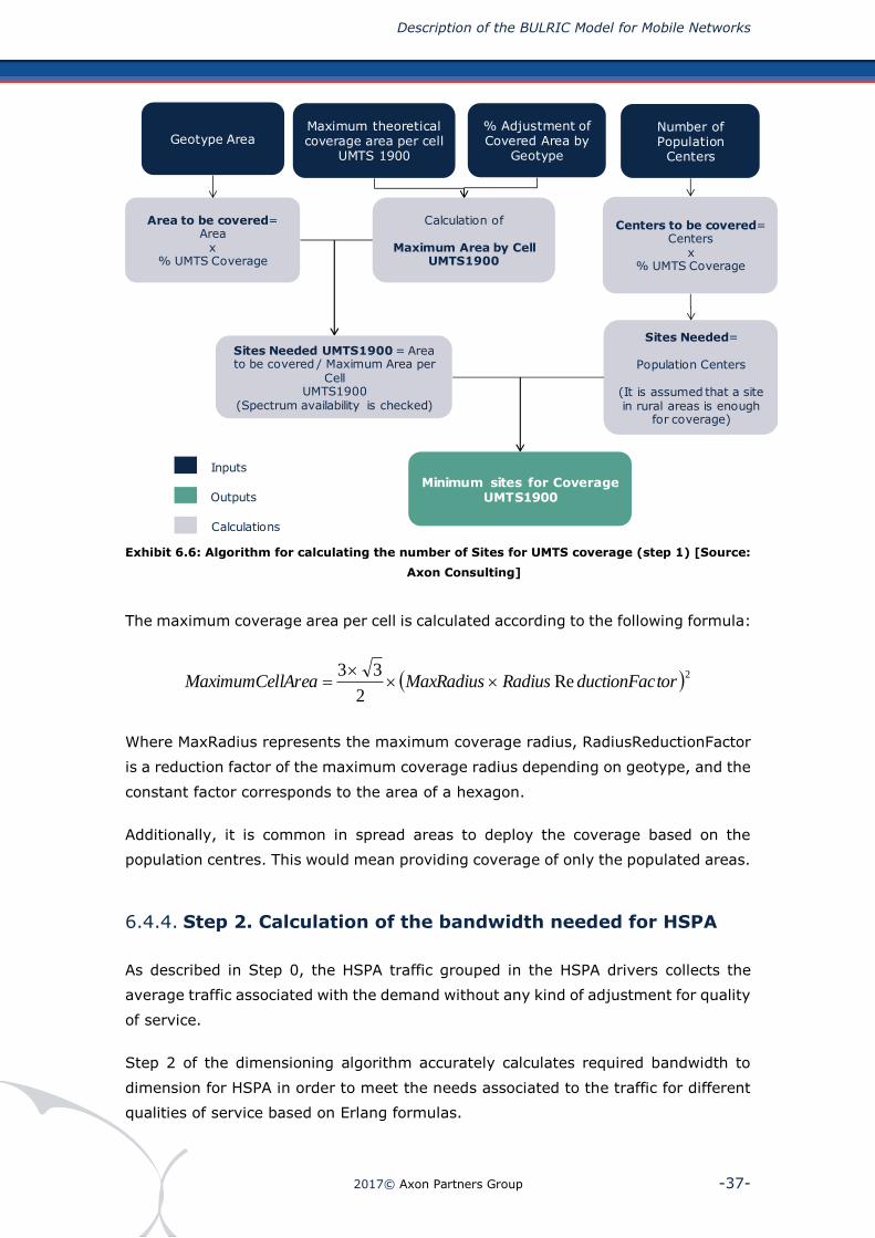
6.4.3. Step 1. Calculating the number of sites required for
coverage
The dimensioning algorithm that calculates the minimum number of sites for UMTS
coverage is similar to that used for GSM. Calculation of equipment requirements for
coverage is worked out for each geotype, generally from the coverage area.
The model is able to calculate the minimum number of sites required for coverage
for 1900MHz band.
The site coverage radius is adjusted based on geotype class, defining a percentage
of the maximum radius as a function of the propagation conditions for each geotype.
The figure below illustrates the calculation of the minimum number of sites associated
with UMTS coverage.
Description of the BULRIC Model for Mobile Networks
2017© Axon Partners Group -37-
Exhibit 6.6: Algorithm for calculating the number of Sites for UMTS coverage (step 1) [Source:
Axon Consulting]
The maximum coverage area per cell is calculated according to the following formula:
2Re
2
33torductionFacRadiusMaxRadiuslAreaMaximumCel
Where MaxRadius represents the maximum coverage radius, RadiusReductionFactor
is a reduction factor of the maximum coverage radius depending on geotype, and the
constant factor corresponds to the area of a hexagon.
Additionally, it is common in spread areas to deploy the coverage based on the
population centres. This would mean providing coverage of only the populated areas.
6.4.4. Step 2. Calculation of the bandwidth needed for HSPA
As described in Step 0, the HSPA traffic grouped in the HSPA drivers collects the
average traffic associated with the demand without any kind of adjustment for quality
of service.
Step 2 of the dimensioning algorithm accurately calculates required bandwidth to
dimension for HSPA in order to meet the needs associated to the traffic for different
qualities of service based on Erlang formulas.
Geotype AreaNumber of Population
Centers
Minimum sites for CoverageUMTS1900
Sites Needed UMTS1900 = Areato be covered / Maximum Area per
CellUMTS1900
(Spectrum availability is checked)
Area to be covered= Area
x % UMTS Coverage
Centers to be covered= Centers
x % UMTS Coverage
Sites Needed=
Population Centers
(It is assumed that a site in rural areas is enough
for coverage)
Maximum theoretical coverage area per cell
UMTS 1900
% Adjustment of Covered Area by
Geotype
Calculation of
Maximum Area by CellUMTS1900
Outputs
Calculations
Inputs

Description of the BULRIC Model for Mobile Networks
2017© Axon Partners Group -38-
The following figure shows the calculation process to obtain the bandwidth needed
for HSPA considering QoS.
Exhibit 6.7: Algorithm for calculating capacity needed for HSPA traffic, considering QoS (step
1) [Source: Axon Consulting]
Please note: Real Time (RT), Gold and Best Effort (BE) refer to different HSPA services
assuring different levels of Quality of Service (QoS).
The calculation is based on the following assumptions:
The needed bandwidth for traffic real time and gold is determined by the adjusted
traffic multiplied by a dimensioning factor. This factor is obtained after apply the
Erlang B formula for real time traffic and Erlang C for gold traffic
Part of the overcapacity allocated to real time and gold traffic (due to the QoS
assurance) can be used for best effort traffic
6.4.5. Step 3. Determination of HSPA release
This step determines the HSPA release considered for radio dimensioning based on
the traffic intensity.
Normalized Capacity UMTS+HSPA BH
Available Spectrum 1900MHz
Number of Sites for Coverage for Traffic=
Number of needed Carriers /
Max. Carriers per Cell/
Sectors per Site
Max. Carriers Available per Cell= Available Spectrum
/
Carrier Bandwidth (5 MHz)
Macro Normalized Capacity= Normalized
Capacity BH x (1 - %micro-pico)
Number of elements radiating Carriers Calculation according to:
Macro Normalized Capacity
Adjusted Pole CapacityMax. Carriers per Cell
Interference Loss FactorNumber of Sites for Coverage
Number of Sectors per Site
Pole Capacity
% Soft Handover(depending on
geotype)
Capacity Reduction Factor for high mobility
(depending on geotype)
Adjusted Pole Capacity=
Pole Capacity
xMobility Factor
/(1+ % Soft Handover)
Interference Loss Factor
Number of Sites for Coverage
Outputs
Calculations
Inputs

Description of the BULRIC Model for Mobile Networks
2017© Axon Partners Group -39-
First and last year of release availability are taken into account. In the last year of
availability all base stations will be updated to subsequent release, independent of
traffic intensity.
6.4.6. Step 4. Calculation of UMTS+HSPA normalised capacity
This step calculates, from total capacity requirements of different bearers of UMTS
and HSPA, a normalised capacity expressed in simultaneous voice users (equivalent
to a channel).
This conversion is based on the concept of "pole capacity" or maximum capacity,
which reflects maximum capacity of an isolated cell equipped with a single carrier in
the event of all traffic belonging to a single bearing capacity. In general, the
maximum capacity of the cell is a reasonably linear function for situations where
traffic from different bearers coexist so that the use of a standard traffic is acceptable.
The figure below illustrates the mechanism used for the calculation of normalised
capacity UMTS+HSPA:
Exhibit 6.8: Algorithm for the calculation of normalised pole capacity. [Source: Axon
Consulting]
Adjusted Traffic Voice CS12.2kbps
Normalized Capacity UMTS =Adjusted Driver Voice CS 12.2 kbps
+ Normalized Capacity CS64 kbps + Normalized Capacity PS64 kbps+ Normalized Capacity PS128 kbps + Normalized Capacity PS384 kbps
Adjusted Driver BH CS64kbps
Normalized Capacity BH CS 64kbps =
Adjusted Trafficx
Pole Capacity CS 64 kbps
/Pole Capacity Voice
Adjusted Driver BH PS64kbps
Normalized Capacity BH HC PS 64kbps =
Adjusted Trafficx
Pole Capacity PS 64 kbps
/Pole Capacity Voice
Adjusted Driver BH PS128kbps
Normalized Capacity BH HC PS 128kbps =
Adjusted Trafficx
Pole Capacity PS 128 kbps
/Pole Capacity Voice
Adjusted Driver BH PS384kbps
Normalized Capacity BH HC PS 384kbps =
Adjusted Trafficx
Pole Capacity PS 384 kbps
/Pole Capacity Voice
Total Normalized Capacity =
Normalized Capacity UMTS+
Normalized Capacity HSPA
Bandwidth Needed HSPA
Release HSPA
Pole Capacity HSPA
Depending on the HSPA Release
Normalized Capacity HSPA =
Bandwidth Needed HSPAx
Pole Capacity HSPA/
Pole Capacity VoiceOutputs CalculationsInputs

Description of the BULRIC Model for Mobile Networks
2017© Axon Partners Group -40-
6.4.7. Step 5. Calculation of the required number of UMTS sites
for macro cells based on traffic
The third step is to determine the number of required UMTS sites to serve voice and
data traffic demand (and their associated signalling requirements.) The illustration
below shows the dimensioning algorithm used for this purpose. This algorithm is used
for different potential configurations of the sites depending on the number of sectors
(3) and the frequency band (1900 MHz) employed.
It is worth noting that the estimation of the number of sites for UMTS is performed
separately for the upstream (UL) and downstream (DL).
Exhibit 6.9: BH Algorithm for calculation of the number of sites for UMTS traffic (step 5)
[Source: Axon Consulting]
Further details of the steps taken to calculate number of sites required:
The total normalised capacity in the dominant busy hour is multiplied by a factor
(1 -% micro) to eliminate the percentage of traffic served by micro cells. This
percentage is dependent on each geotype
The maximum capacity of an isolated cell (Pole Capacity) is adjusted to take into
consideration the impact of Soft Handover and loss of capacity for mobility
Normalized Capacity UMTS+HSPA BH
Available Spectrum 1900MHz
Number of Sites for Coverage for Traffic=
Number of needed Carriers /
Max. Carriers per Cell/
Sectors per Site
Max. Carriers Available per Cell= Available Spectrum
/
Carrier Bandwidth (5 MHz)
Macro Normalized Capacity= Normalized
Capacity BH x (1 - %micro-pico)
Number of elements radiating Carriers Calculation according to:
Macro Normalized Capacity
Adjusted Pole CapacityMax. Carriers per Cell
Interference Loss FactorNumber of Sites for Coverage
Number of Sectors per Site
Pole Capacity
% Soft Handover(depending on
geotype)
Capacity Reduction Factor for high mobility
(depending on geotype)
Adjusted Pole Capacity=
Pole Capacity
xMobility Factor
/(1+ % Soft Handover)
Interference Loss Factor
Number of Sites for Coverage
Outputs
Calculations
Inputs

Description of the BULRIC Model for Mobile Networks
2017© Axon Partners Group -41-
(especially important in road or rail class geotypes). This maximum adjusted
capacity is called Pole Capacity adjusted
It must be taken into account that in UMTS, as carrier frequencies are reused in
cells attached for traffic growth, the maximum capacity per carrier tends to
decrease as a result of the interference. In the model, this effect is reflected as
follows:
Equation A:
Where the Interference Loss Factor is the ratio between the maximum capacity
of a carrier in a "multiple cell" (all adjacent cells use the same carrier) and the
maximum capacity of the cell in an environment of “single cell” or solitary
confinement.
I𝑛𝑡𝑒𝑟𝑓𝑒𝑟𝑒𝑛𝑐𝑒𝐿𝑜𝑠𝑠𝐹𝑎𝑐𝑡𝑜𝑟 =𝑃𝑜𝑙𝑒𝐶𝑎𝑝𝑎𝑐𝑖𝑡𝑦𝐶𝑎𝑟𝑟𝑖𝑒𝑟𝑀𝑢𝑙𝑡𝑖𝑝𝑙𝑒𝐶𝑒𝑙𝑙
𝑃𝑜𝑙𝑒𝐶𝑎𝑝𝑎𝑐𝑖𝑡𝑦𝐶𝑎𝑟𝑟𝑖𝑒𝑟𝑆𝑖𝑛g𝑙𝑒𝐶𝑒𝑙𝑙
From this, it is possible to determine the number of required carriers (radiating
elements) to meet total traffic. The number of traffic carriers comes from the
following expression:
Equation B
N𝑢𝑚𝑏𝑒𝑟 𝑜𝑓 𝑇𝑟𝑎𝑓𝑓𝑖𝑐 𝐶𝑎𝑟𝑟𝑖𝑒𝑟s =𝑇𝑜𝑡𝑎𝑙𝑁𝑜𝑟𝑚𝑎𝑙𝑖𝑧𝑒𝑑𝐶𝑎𝑝𝑎𝑐𝑖𝑡𝑦
𝐶𝑎𝑝𝑎𝑐𝑖𝑡𝑦𝑃𝑒𝑟𝐶𝑎𝑟𝑟𝑖𝑒𝑟
In this case, the number of sites required is given by:
S𝑖𝑡𝑒𝑠 =𝑁𝑢𝑚𝑏𝑒𝑟 𝑜𝑓 𝑇𝑟𝑎𝑓𝑓𝑖𝑐 𝐶𝑎𝑟𝑟𝑖𝑒𝑟𝑠
𝑀𝑎𝑥𝐶𝑎𝑟𝑟𝑖𝑒𝑟𝑠𝑃𝑒𝑟𝑆𝑒𝑐𝑡𝑜𝑟
6.4.8. Step 6. Calculation of optimal configuration and number
of sites
Step 6 of the dimensioning algorithm determines the appropriate configuration,
based on the number of sites required in Step 5.
In the calculation in Step 5, both traffic and coverage requirements are already
considered. Minimum configuration is considered as that which minimises the number
of necessary sites, as it is assumed that the costs associated with construction and
maintenance of the site are the most significant of the radio access network.
)Re%1( orceLossFactInterferenuseFrequencyedtyNormalizPoleCapacirCarrierCapacityPe

Description of the BULRIC Model for Mobile Networks
2017© Axon Partners Group -42-
6.4.9. Step 7. Calculation of the number of macro network
elements
Once the number of required sites is determined, along with the corresponding
configuration, Step 7 calculates the number of necessary macro network elements.
These include the number of base stations (which can support both cards, 700-900
MHz and 2100 MHz, at the same time) and the number of carriers. Please note that
base stations split into bi- and tri-sector.
The figure below illustrates the calculation algorithm used for determining the
number of necessary macro network elements:
Exhibit 6.10: Algorithm for calculation of the number of macro network elements. (Step 7)
[Source: Axon Consulting]
The following aspects, when applicable, are of interest in connection with the
algorithm for calculating the number of macro network elements:
Number of Sites Needed
Minimum Carriers UMTS900 = NodesB
UMTS 900 x Sectors per Cell
X Operators RAN sharing
Initial Number of NodesB
UMTS 1900 = Number of Sites 900
Carriers UMTS 1900 Needed
(maximum of the two)
NodesB Extra (saturation) =
Carriers UMTS Needed / Max. Carriers per
NodeB – NodesB UMTS initial
NodesB UMTS = NodesB UMTS initial + NodesB UMTS extra
Carriers UMTS 1900
Outputs
Calculation
Inputs
Total Carriers Needed for Traffic

Description of the BULRIC Model for Mobile Networks
2017© Axon Partners Group -43-
The algorithm takes into account that each location must have at least one base
station. At least one carrier per sector is required
If the number of carriers per base station exceeds the limit that supports the base
station (technical limitations), it is assumed that new Nodes B equipment will
need to be installed in order to accommodate additional carriers. These Nodes B
are called "additional" nodes B in the previous chart
6.4.10. Step 8. Calculation of the quantity of HSPA Equipment
Needed (SW enabling)
Step 8 of the dimensioning algorithm determines the amount of necessary equipment
(software enabling or licenses) to cover HSPA services’ traffic.
In general, the number of Nodes B requiring an HSPA software update is provided by
the following formula:
TSCoverageUM
PACoverageHSNodesBNodesBHSPA
%
%
The software release is determined in Step 3.
The figure below illustrates the calculation algorithm for determining the number of
necessary HSPA upgrades.
Exhibit 6.11: Algorithm for calculation of the number of HSPA upgrades necessary (step 8)
[Source: Axon Consulting]
NodesB Number
Number of Equipment with Release HSPA =
NodesB NumberX
% HSPA Equipments(only for the chosen Release, 0 for the rest)
% HSPA Coverage
% HSPA Equipments = % Coverage HSPA /% Coverage UMTS
Appropriate HSPA Release
% UMTS Coverage
Outputs
Calculations
Inputs
Description of the BULRIC Model for Mobile Networks
2017© Axon Partners Group -44-
6.5. Radio access dimensioning LTE
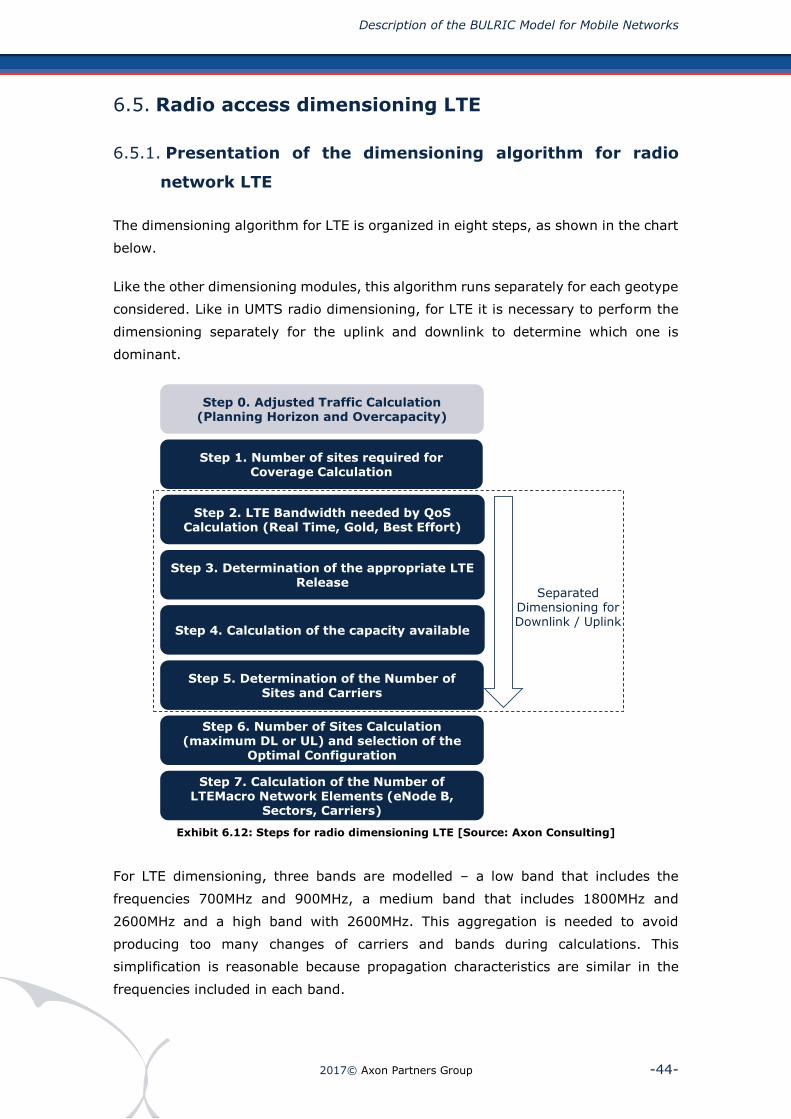
6.5.1. Presentation of the dimensioning algorithm for radio
network LTE
The dimensioning algorithm for LTE is organized in eight steps, as shown in the chart
below.
Like the other dimensioning modules, this algorithm runs separately for each geotype
considered. Like in UMTS radio dimensioning, for LTE it is necessary to perform the
dimensioning separately for the uplink and downlink to determine which one is
dominant.
Exhibit 6.12: Steps for radio dimensioning LTE [Source: Axon Consulting]
For LTE dimensioning, three bands are modelled – a low band that includes the
frequencies 700MHz and 900MHz, a medium band that includes 1800MHz and
2600MHz and a high band with 2600MHz. This aggregation is needed to avoid
producing too many changes of carriers and bands during calculations. This
simplification is reasonable because propagation characteristics are similar in the
frequencies included in each band.
Step 0. Adjusted Traffic Calculation(Planning Horizon and Overcapacity)
Step 2. LTE Bandwidth needed by QoS Calculation (Real Time, Gold, Best Effort)
Step 1. Number of sites required for Coverage Calculation
Step 5. Determination of the Number of Sites and Carriers
Step 7. Calculation of the Number of LTEMacro Network Elements (eNode B,
Sectors, Carriers)
Step 8. Calculation of the Number of Micro/Pico
Network Elements
Step 4. Calculation of the capacity available
Step 6. Number of Sites Calculation (maximum DL or UL) and selection of the
Optimal Configuration
Step 3. Determination of the appropriate LTE Release
SeparatedDimensioning forDownlink / Uplink

Description of the BULRIC Model for Mobile Networks
2017© Axon Partners Group -45-
For the capacity dimensioning, the carriers’ separation is maintained to obtain the
actual capacity. For instance, in the of case an operator who has 5MHz in the 800MHz
band and 10MHz in the 900MHz band, the model recognises that there is one 5MHz
carrier and one 10MHz carriers in the low band (and not one 15MHz carrier).
Each step is described in further detail in the following sections.
6.5.2. Step 0. Adjusted traffic calculation (planning horizon and
efficiency factor)
A preliminary step to dimensioning an LTE network is the calculation of the traffic
network dependent. In the calculation of this traffic, denominated "adjusted traffic“,
two factors are involved:
1. The effect of the planning horizon.
2. Overcapacity for security reasons.
The LTE radio network dimensioning in terms of traffic is carried out from the drivers
listed below:
DRIV.LTE.Data LTE-B.Best Effort-DL
DRIV.LTE.Data LTE-QoS.Gold-DL
DRIV.LTE.Data LTE-QoS.Real Time-DL
DRIV.LTE.Data LTE-B.Best Effort-UL
DRIV.LTE.Data LTE-QoS.Gold-UL
DRIV.LTE.Data LTE-QoS.Real Time-UL
DRIV.LTE.SIGNAL.SIGNAL
Drivers are split into sub sections according to their qualities of service and
signalling9. For each of these types, a differentiation between uplink (UL) and
downlink (DL) has been introduced.
The following aspects are of particular interest:
9 Channel switched services (i.e. voice, video calls) is managed as data traffic by the LTE network, ensuring that the QoS is adequate for those services. Therefore, the CS services have been allocated to the drivers related to real time traffic.

Description of the BULRIC Model for Mobile Networks
2017© Axon Partners Group -46-
The mapping of voice and video telephony LTE is performed similarly to the
mapping of UMTS services. That is, adding a percentage of "idle" or inactive traffic
to represent time unbilled but during which the network is used (such as the time
until the recipient picks up the phone and calls not answered). To this "increased”
traffic a factor is applied to calculate the number of channels required (according
to the Erlang B formula) for a given blocking probability
Referring to the services mapped on drivers of LTE data services, an over sizing
factor representing the necessary retransmissions due to errors in the channel is
taken into account. In addition to these parameters, an "idle" occupancy rate of
the channel to model the times during which the user is assigned a channel but
not transmitting or receiving any data is considered.
The busy hour rate applies to all the drivers outlined above and, for voice and video
calls, the factor of radio access service is used, depending on whether the service is
on-net (using the radio network at both ends of the communication) or off-net (using
a single communication endpoint).
6.5.3. Step 1. Calculating the number of sites required for
coverage
The dimensioning algorithm for the minimum number of sites for LTE coverage is
similar to that used for UMTS and GSM. The calculation of equipment requirements
for coverage is carried out for each geotype, generally from the coverage area.
The model is able to calculate the minimum number of sites required for coverage
for all the bands. In the case of LTE, as it has been stated before, the model considers
three bands: low (800MHz and 900MHz), medium (1800MHz and 2600MHz) and high
(2600MHz).
The site coverage radius is adjusted based on geotype class, defining a percentage
of the maximum radius as a function of the propagation conditions for each geotype.
The figure below illustrates the calculation of the minimum number of sites associated
with LTE coverage:
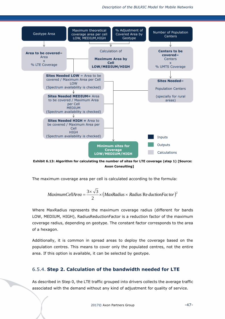
Description of the BULRIC Model for Mobile Networks
2017© Axon Partners Group -47-
Exhibit 6.13: Algorithm for calculating the number of sites for LTE coverage (step 1) [Source:
Axon Consulting]
The maximum coverage area per cell is calculated according to the formula:
2Re
2
33torductionFacRadiusMaxRadiuslAreaMaximumCel
Where MaxRadius represents the maximum coverage radius (different for bands
LOW, MEDIUM, HIGH), RadiusReductionFactor is a reduction factor of the maximum
coverage radius, depending on geotype. The constant factor corresponds to the area
of a hexagon.
Additionally, it is common in spread areas to deploy the coverage based on the
population centres. This means to cover only the populated centres, not the entire
area. If this option is available, it can be selected by geotype.
6.5.4. Step 2. Calculation of the bandwidth needed for LTE
As described in Step 0, the LTE traffic grouped into drivers collects the average traffic
associated with the demand without any kind of adjustment for quality of service.
Geotype Area Number of Population Centers
Sites Needed MEDIUM= Area to be covered / Maximum Area
per CellMEDIUM
(Spectrum availability is checked)
Minimum sites for Coverage
LOW/MEDIUM/HIGH
Sites Needed LOW = Area to be covered / Maximum Area per Cell
LOW(Spectrum availability is checked)
Area to be covered= Area
x % LTE Coverage
Centers to be covered= Centers
x % UMTS Coverage
Sites Needed=
Population Centers
(specially for rural areas)
Maximum theoretical coverage area per cell LOW, MEDIUM,HIGH
% Adjustment of Covered Area by
Geotype
Calculation of
Maximum Area by Cell
LOW/MEDIUM/HIGH
Outputs
Calculations
Inputs
Sites Needed HIGH = Area to be covered / Maximum Area per
CellHIGH
(Spectrum availability is checked)
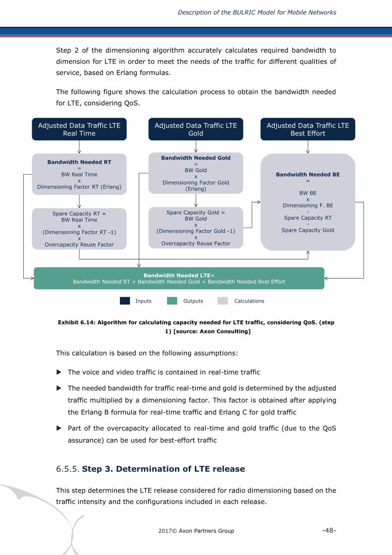
Description of the BULRIC Model for Mobile Networks
2017© Axon Partners Group -48-
Step 2 of the dimensioning algorithm accurately calculates required bandwidth to
dimension for LTE in order to meet the needs of the traffic for different qualities of
service, based on Erlang formulas.
The following figure shows the calculation process to obtain the bandwidth needed
for LTE, considering QoS.
Exhibit 6.14: Algorithm for calculating capacity needed for LTE traffic, considering QoS. (step
1) [source: Axon Consulting]
This calculation is based on the following assumptions:
The voice and video traffic is contained in real-time traffic
The needed bandwidth for traffic real-time and gold is determined by the adjusted
traffic multiplied by a dimensioning factor. This factor is obtained after applying
the Erlang B formula for real-time traffic and Erlang C for gold traffic
Part of the overcapacity allocated to real-time and gold traffic (due to the QoS
assurance) can be used for best-effort traffic
6.5.5. Step 3. Determination of LTE release
This step determines the LTE release considered for radio dimensioning based on the
traffic intensity and the configurations included in each release.
Outputs CalculationsInputs
Adjusted Data Traffic LTEReal Time
Bandwidth Needed LTE=Bandwidth Needed RT + Bandwidth Needed Gold + Bandwidth Needed Best Effort
Bandwidth Needed RT =
BW Real Time x
Dimensioning Factor RT (Erlang)
Spare Capacity RT = BW Real Time
x (Dimensioning Factor RT -1)
x Overcapacity Reuse Factor
Adjusted Data Traffic LTEGold
Bandwidth Needed Gold=
BW Goldx
Dimensioning Factor Gold (Erlang)
Spare Capacity Gold = BW Gold
x (Dimensioning Factor Gold -1)
x Overcapacity Reuse Factor
Adjusted Data Traffic LTEBest Effort
Bandwidth Needed BE=
BW BEx
Dimensioning F. BE-
Spare Capacity RT-
Spare Capacity Gold
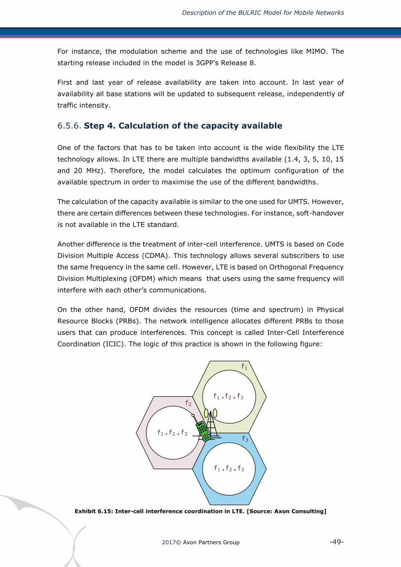
Description of the BULRIC Model for Mobile Networks
2017© Axon Partners Group -49-
For instance, the modulation scheme and the use of technologies like MIMO. The
starting release included in the model is 3GPP’s Release 8.
First and last year of release availability are taken into account. In last year of
availability all base stations will be updated to subsequent release, independently of
traffic intensity.
6.5.6. Step 4. Calculation of the capacity available
One of the factors that has to be taken into account is the wide flexibility the LTE
technology allows. In LTE there are multiple bandwidths available (1.4, 3, 5, 10, 15
and 20 MHz). Therefore, the model calculates the optimum configuration of the
available spectrum in order to maximise the use of the different bandwidths.
The calculation of the capacity available is similar to the one used for UMTS. However,
there are certain differences between these technologies. For instance, soft-handover
is not available in the LTE standard.
Another difference is the treatment of inter-cell interference. UMTS is based on Code
Division Multiple Access (CDMA). This technology allows several subscribers to use
the same frequency in the same cell. However, LTE is based on Orthogonal Frequency
Division Multiplexing (OFDM) which means that users using the same frequency will
interfere with each other’s communications.
On the other hand, OFDM divides the resources (time and spectrum) in Physical
Resource Blocks (PRBs). The network intelligence allocates different PRBs to those
users that can produce interferences. This concept is called Inter-Cell Interference
Coordination (ICIC). The logic of this practice is shown in the following figure:
Exhibit 6.15: Inter-cell interference coordination in LTE. [Source: Axon Consulting]
f1
f1 + f2 + f3
f3
f1 + f2 + f3
f2
f1 + f2 + f3

Description of the BULRIC Model for Mobile Networks
2017© Axon Partners Group -50-
Although this technique enables the avoidance of interference when using the same
frequencies in all the cells, the maximum bit rate reached in the cell borders will be
lower than expected. Therefore, the model considers a factor that represents the
average decrease in capacity that can be handled by the eNode B.
The following figure shows the calculation process for the adjusted capacity available.
Exhibit 6.16: Calculation of the adjusted capacity available. [Source: Axon Consulting]
6.5.7. Step 5. Calculation of the required number of LTE sites for
macro cells based on traffic
For the calculation of LTE sites for macro sites, the model implements the same
methodology used for GSM and UMTS networks (described in sections 6.3.4 and
6.4.7, respectively). However, for LTE three bands have been defined (LOW,
MEDIUM, HIGH). Therefore, the model considers three variables, instead of two.
The following exhibit shows the calculation process for the sites needed for each
band:
Theoretical Capacity per Cell based on the frequency and
the bandwidth available
Bandwidth available in band LOW/MEDIUM/HIGH
Adjusted capacity =Theoretical Capacity * Frequency reutilisationfactor * Mobility Factor
Capacity in configurations
available
Frequency reutilisation factorFactor for the consideration of the mobility of the users
Outputs
Calculations
Inputs

Description of the BULRIC Model for Mobile Networks
2017© Axon Partners Group -51-
Exhibit 6.17: Calculation algorithm of the required sites for traffic LTE by band [Source: Axon
Consulting]
6.5.8. Step 6. Calculation of optimal configuration and number
of sites
Step 6 of the dimensioning algorithm determines the appropriate configuration based
on the number of sites required in Step 5.
In the calculation in Step 5, both traffic and coverage requirements are already
considered. The minimum configuration is considered as that which minimises the
number of necessary sites, as it is assumed that the costs associated with
construction and maintenance of the site are the most significant.
6.5.9. Step 7. Calculation of the number of macro network
elements
Once the number of required sites is determined, along with the corresponding
configuration, Step 7 calculates the number of necessary macro network elements.
These include the number of base stations (eNode B) and the number of carriers.
Please note that base stations are split between bi and tri-sector.
The figure below illustrates the calculation algorithm used for determining the
number of necessary macro network elements:
Maximum bandwidth LTE FDD DL
Bandwidth needed FDD DL=
Max. BW LTE BHx
(1 - %micro)
Needed sites for Traffic – Band LOW=Max(UL, DL)
Needed sites for Traffic – Band MEDIUM=Max(UL, DL)
Needed sites for Traffic – Band HIGH=Max(UL, DL)
Adjusted Capacity LTE FDD DL for bands L/M/H
Maximum bandwidth LTE FDD UL
Bandwidth needed FDD DL=
Max. BW LTE BHx
(1 - %micro)
Adjusted Capacity LTE FDD UL for bands L/M/H
Sites needed= BW needed/Adj. Capacity
Sites needed= BW needed/Adj. Capacity
Outputs
Calculations
Inputs

Description of the BULRIC Model for Mobile Networks
2017© Axon Partners Group -52-
Exhibit 6.18: Algorithm for Calculation of the number of LTE macro network elements (Step 7)
[source: Axon Consulting]
6.6. Radio sites dimensioning
The radio sites dimensioning block is responsible for the calculation of the required
number of sites. Additionally, this block obtains the number of necessary antennas
for each technology.
When designing the access network for different technologies an indicator of the
number of sites required for each band is obtained. However, it is common practice
among operators to reuse the site to co-locate the equipment of different bands and
technologies, thus cutting costs.
For the dimensioning of sites the following steps apply:
Exhibit 6.19: Steps for calculating the co-location of radio sites. [source: Axon Consulting]
Throughout the following subsections the three steps shown in the figure above are
explained in detail.
Number of LTE sites Bandwidth needed
Bandwidth per site needed
Optimum Configuration
Capacities per Carrier available
Number of carriers needed per site
Maximum carriers per eNodeB
Number of eNodeBs per site=
Needed carriers per site / maximum carriers per
eNodeB
Total Number of LTE Equipment=
LTE Equipment per Site* LTE sites
Outputs
Calculations
Inputs
Step 1. Technologies Co-location
Step 2. Total number of Sites Calculation
Step 3. Number of Antennas Calculation

Description of the BULRIC Model for Mobile Networks
2017© Axon Partners Group -53-
6.6.1. Technology co-location
Once the number of radio sites needed for each technology (from radio dimensioning
modules) is known, the co-location between different technologies is estimated.
These data need to be differentiated between tower-roof locations (which will be
separated later) and micro-cell sites.
These sites may be co-located, producing the following combinations:
GSM+UMTS+LTE
GSM + UMTS
UMTS + LTE
GSM + LTE
GSM Only
UMTS Only
LTE Only
To group the locations in all possible combinations the algorithm shown in the picture
below has been followed. Notably, this is done separately for tower-roof locations (on
one side) and micro (on the other).

Description of the BULRIC Model for Mobile Networks
2017© Axon Partners Group -54-
Exhibit 6.20: Algorithm used for the calculation of technology co-location [source: Axon
Consulting]
The steps followed throughout the algorithm are outlined below:
1. Calculation of the co-location sites with the three technologies. To do this,
the minimum of the three technologies is taken and a maximum
percentage of maximum co-location is applied.
2. Calculation of the number of sites not yet co-located for each technology.
3. Calculation of the co-location sites of UMTS and GSM, taking the minimum
of the remaining sites and applying a factor of maximum percentage of
co-location.
4. Calculation of the number of sites not yet co-located for each technology.
Micro SitesMacro Sites
SITESGSM
SITESUMTS
SITESLTE
MINSITES
GSM+UMTS+LTE
REMAINING GSM SITES
REMAINING UMTS SITES
REMAINING LTE SITES
SITESGSM+UMTS
MIN
REMAINING GSM SITES
REMAINING UMTS SITES
REMAINING LTE SITES
MIN
REMAINING GSM SITES
REMAINING UMTS SITES
REMAINING LTE SITES
SITES GSM+LTE
MIN
REMAINING GSM SITES
REMAINING UMTS SITES
REMAINING LTE SITES
SITESUMTS+LTE
SITESGSM ONLY
SITESUMTS ONLY
SITES LTE ONLY
SITESGSM
SITESUMTS
SITESLTE
MIN
REMAINING GSM SITES
REMAINING UMTS SITES
REMAINING LTE SITES
MIN
REMAINING GSM SITES
REMAINING UMTS SITES
REMAINING LTE SITES
MIN
REMAINING GSM SITES
REMAINING UMTS SITES
REMAINING LTE SITES
MIN
REMAINING GSM SITES
REMAINING UMTS SITES
REMAINING LTE SITES
SITESGSM ONLY
SITESUMTS ONLY
SITESLTE ONLY
Outputs CalculationsInputs
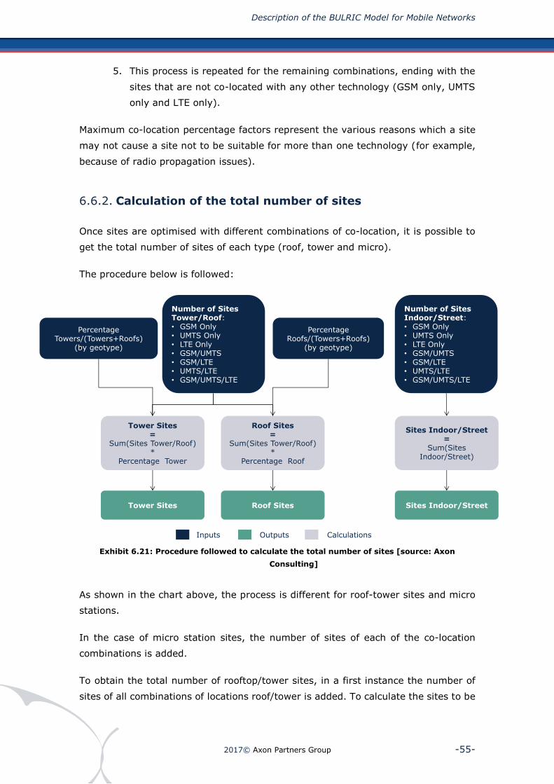
Description of the BULRIC Model for Mobile Networks
2017© Axon Partners Group -55-
5. This process is repeated for the remaining combinations, ending with the
sites that are not co-located with any other technology (GSM only, UMTS
only and LTE only).
Maximum co-location percentage factors represent the various reasons which a site
may not cause a site not to be suitable for more than one technology (for example,
because of radio propagation issues).
6.6.2. Calculation of the total number of sites
Once sites are optimised with different combinations of co-location, it is possible to
get the total number of sites of each type (roof, tower and micro).
The procedure below is followed:
Exhibit 6.21: Procedure followed to calculate the total number of sites [source: Axon
Consulting]
As shown in the chart above, the process is different for roof-tower sites and micro
stations.
In the case of micro station sites, the number of sites of each of the co-location
combinations is added.
To obtain the total number of rooftop/tower sites, in a first instance the number of
sites of all combinations of locations roof/tower is added. To calculate the sites to be
Number of SitesTower/Roof:• GSM Only• UMTS Only• LTE Only• GSM/UMTS• GSM/LTE• UMTS/LTE• GSM/UMTS/LTE
Tower Sites
Tower Sites=
Sum(Sites Tower/Roof)*
Percentage Tower
Number of SitesIndoor/Street:• GSM Only• UMTS Only• LTE Only• GSM/UMTS• GSM/LTE• UMTS/LTE• GSM/UMTS/LTE
PercentageTowers/(Towers+Roofs)
(by geotype)
PercentageRoofs/(Towers+Roofs)
(by geotype)
Roof Sites=
Sum(Sites Tower/Roof)*
Percentage Roof
Sites Indoor/Street=
Sum(SitesIndoor/Street)
Roof Sites Sites Indoor/Street
Outputs CalculationsInputs

Description of the BULRIC Model for Mobile Networks
2017© Axon Partners Group -56-
placed on rooftops and on towers, the actual percentage of installed sites for each
type and for each geotype is then considered.
6.7. Backhaul network dimensioning
6.7.1. Introduction to backhaul dimensioning
The backhaul module is responsible for dimensioning the transmission part of radio
sites to the controllers (BSC, RNC) along with the dimensioning of controlling
elements. The backhaul dimensioning algorithm is implemented in the ‘6E CALC DIM
BACKHAUL’ sheet of the model.
The topology used for the backhaul network is based on the following structure:
Radio Site – Hub: a connection point to point from radio sites to a traffic
aggregator equipment (hub). The percentage of radio sites that connect directly
to the controller may be configured
The definition of the topology to be used is made for each geotype and differentiates
between microwave and fibre (leased line option is always considered point to point).
Topology is defined by two parameters:
Number of aggregation (N) represents the number of aggregators in the ring. The
case of N = 1 represents the point to point topology
Redundancy factor (R) can be 1 or 0. When this parameter is configured to 1, the
network will have redundancy. Please note that to set a ring topology, R must be
equal to 1
The following illustrations show the network topologies that can be used in the model:

Description of the BULRIC Model for Mobile Networks
2017© Axon Partners Group -57-
Exhibit 6.22: Topology scheme for backhaul network with point-to-point links. [source: Axon
Consulting]
Radio Site Hub Controller

Description of the BULRIC Model for Mobile Networks
2017© Axon Partners Group -58-
Exhibit 6.23: Topology scheme for backhaul network with ring connection between hubs and
the controller [Source: Axon Consulting]
As shown in the chart, the elements considered in the backhaul network topology
are:
Transmission links between radio site and the hub or the controller, which may
use a mix of different technologies (microwave, leased lines or fibre)
Hubs or backbone centres: the traffic from radio sites is added in this element.
The aggregator is placed in the location of a radio site hence there being a direct
link
Controllers: these include controllers of different technologies (GSM for BSC, RNC
for UMTS and switches for LTE). The locations are shared by all three technologies
and, similarly to the aggregators, controllers are located in a shared location with
a radio site and an aggregator in the same location of a core site
Radio Site Hub Controller

Description of the BULRIC Model for Mobile Networks
2017© Axon Partners Group -59-
6.7.2. Dimensioning algorithm for backhaul network
The dimensioning algorithm for a backhaul network is organised into six steps, as
shown in the illustration below.
It is important to clarify that, like the other dimensioning modules this algorithm runs
separately for each geotype considered.
In the case of steps 2 and 3, the algorithm also runs for each node type (i.e., in the
case of base stations with GSM, GSM and UMTS, etc.) and link type (radio hub
location).
Exhibit 6.24: Steps for backhaul dimensioning. [Source: Axon Consulting]
6.7.3. Step 1. Calculation of requested capacities
In Step 2 the backhaul transmission requirements for each type of site are calculated.
That is, radio sites are distinguished between those with only GSM technology, those
with only UMTS radio and so on. This process is carried out differently for radio site-
backbone centres links, hence the need for the following step.
Step 1. Calculation of requestedcapacities for radio site typologies
Step 2. Cost calculation by link type and technology
Step 3. Determination of the optimumconfiguration
Step 4. Data consolidation
Step 5. Determination of neededBackhaul network equipment
Steps 2-3 repeated for
each node typeand connection

Description of the BULRIC Model for Mobile Networks
2017© Axon Partners Group -60-
Calculation of required capacities for radio site – Hub (Backbone centres)
links
To determine the capacity (bandwidth) required of the links between the radio site
and hub, the model first calculates average bandwidth per base station type
depending on the number of sites and bandwidth required, by technology10.
Having calculated the average bandwidth required for GSM, UMTS and LTE base
station, the capacity is determined for each type of site as the sum of the capacities
located on the site, as shown in the illustration below11:
Exhibit 6.25: Calculation of required capacity by radio site typology. [Source: Axon
Consulting]
10 Note that for the conversion of voice and/or video minutes bit rates are used, and they may differ from those in the radio access. 11 Note that in all cases a minimum granularity of links needed by technology is considered. This is to prevent combined GSM and UMTS traffic within a single E1 for example, because traffic will not be added at that level.
GSM Bandwidth (MBps)
Total Sites GSM
Average bandwidth per GSM site =
Total Bandwidth/ Total Sites
UMTS Bandwidth (MBps)
Total Sites UMTS
Average bandwidth per UMTS site =
Total Bandwidth/ Total Sites
LTE Bandwidth (MBps)
Total Sites LTE
Average bandwidth per LTE site =
Total Bandwidth/ Total Sites
Required capacity GSM site
Required capacity GSM + UMTS site
Required capacity GSM + UMTS + LTE site
Required capacity GSM + LTE site
Required capacity UMTS site
Required capacity UMTS + LTE site
Required capacity LTE site
Outputs
Calculations
Inputs

Description of the BULRIC Model for Mobile Networks
2017© Axon Partners Group -61-
6.7.4. Step 2. Cost calculation by link and technology
In Step 2 costs associated to all links are determined. This calculation is performed
for each link and for each type of technology (leased lines, fibre optic and
microwave).
The model first calculates the number of links required by each technology and bit
rate available. Once the number of each link that is needed to satisfy the required
capacity is determined, their cost is calculated.
For each technology (microwave, leased lines and fibre optic), the most cost efficient
option is selected (e.g. two E1 may be cheaper than one E3).
The illustration below shows the calculation process regarding links necessary for
each type of technology:
Exhibit 6.26: Calculation of optimum configuration of links needed (for each technology
separately) [Source: Axon Consulting]
6.7.5. Step 3. Determination of the optimal backhaul network
In step three the network configuration is optimised from a costing point of view,
taking into consideration a technical availability factor for each of the technologies
considered.
For instance, leased lines may not be available in certain geotypes or it is not possible
to use microwaves for all the sites in a geotype due to technical issues (e.g.
mountainous regions).
CapacityLink length
Links Number (i) = Roundup(Capacity/Bitrate(i))
Optimum Configuration Per technology=Min(Cost(i))
Unitary costs by linkBitrates
Cost(i)=Links Number
(i)*CostPerLink(i) +Links Number(i)*
Distance*CostPerKm(i)
Outputs
Calculations
Inputs
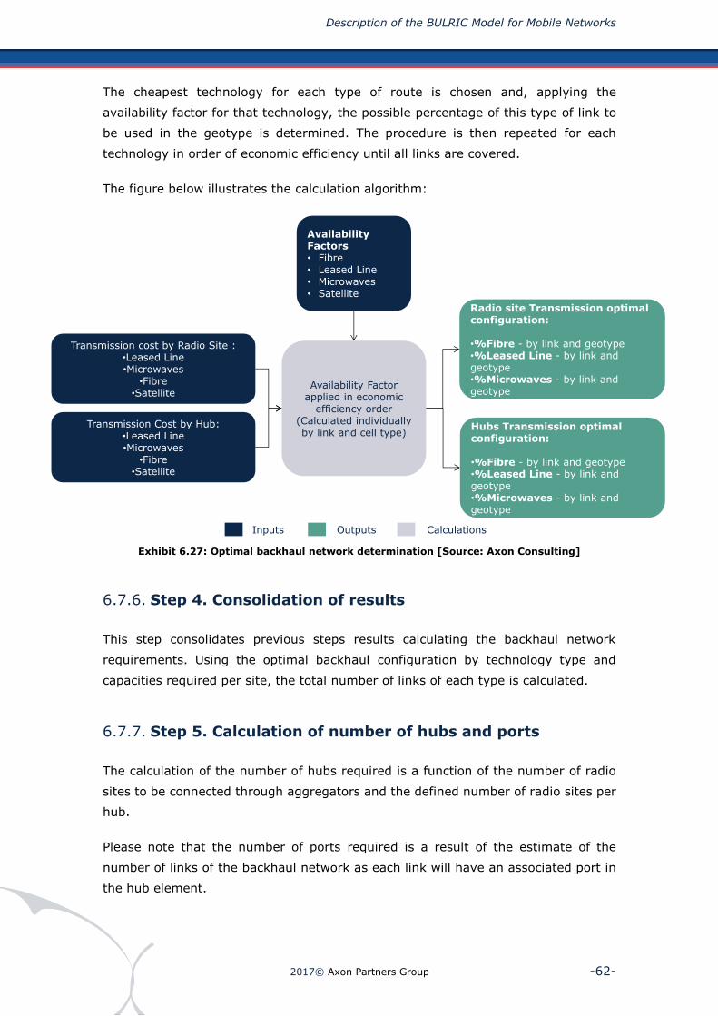
Description of the BULRIC Model for Mobile Networks
2017© Axon Partners Group -62-
The cheapest technology for each type of route is chosen and, applying the
availability factor for that technology, the possible percentage of this type of link to
be used in the geotype is determined. The procedure is then repeated for each
technology in order of economic efficiency until all links are covered.
The figure below illustrates the calculation algorithm:
Exhibit 6.27: Optimal backhaul network determination [Source: Axon Consulting]
6.7.6. Step 4. Consolidation of results
This step consolidates previous steps results calculating the backhaul network
requirements. Using the optimal backhaul configuration by technology type and
capacities required per site, the total number of links of each type is calculated.
6.7.7. Step 5. Calculation of number of hubs and ports
The calculation of the number of hubs required is a function of the number of radio
sites to be connected through aggregators and the defined number of radio sites per
hub.
Please note that the number of ports required is a result of the estimate of the
number of links of the backhaul network as each link will have an associated port in
the hub element.
Availability Factors• Fibre• Leased Line• Microwaves• Satellite
Transmission cost by Radio Site :•Leased Line•Microwaves
•Fibre•Satellite
Transmission Cost by Hub:•Leased Line•Microwaves
•Fibre•Satellite
Radio site Transmission optimal configuration:
•%Fibre - by link and geotype•%Leased Line - by link and geotype•%Microwaves - by link and geotype
Availability Factor applied in economic
efficiency order(Calculated individually by link and cell type)
Hubs Transmission optimal configuration:
•%Fibre - by link and geotype•%Leased Line - by link and geotype•%Microwaves - by link and geotype
Outputs CalculationsInputs
Description of the BULRIC Model for Mobile Networks
2017© Axon Partners Group -63-
6.8. Core network dimensioning
6.8.1. Introduction to core network dimensioning
The core network dimensioning module is responsible for the dimensioning of the
backbone network and core equipment, dealing with the central network
management.
The model defines two fundamental phases for the core network:
First phase: the core network is formed by equipment 3Gpp legacy equipment,
including the separation of the control and traffic layers (MSC-S+MGW). First-
phase core is adequate for GSM and UMTS
Second phase: this phase represents the evolved core. The evolved core has the
necessary equipment to support LTE Access networks and is based on All-IP
transmission. Additionally, it includes IMS equipment for supporting services
generated by 2G and 3G access networks
The change between first and second phases is carried out in the year selected in the
control panel (“no migration” option is also available). However, if an LTE network is
developed, the creation of an evolved core is needed. Therefore, the two cores can
coexist from the year when the LTE access network starts to be rolled-out and the
year selected for the migration of the core network.
Description of core architecture
The following illustration shows the traditional network structure (first phase) from a
functional viewpoint:

Description of the BULRIC Model for Mobile Networks
2017© Axon Partners Group -64-
Exhibit 6.28: Schematic model of traditional network. [Source: Axon Consulting]
The main equipment making up the traditional core network is:
MSC-S (Mobile Switching Centre Server): the MSC-S is responsible for
managing the control of circuit call level in the mobile network, i.e. voice and
video calls. The MSC manages signalling issues, user mobility and call control. It
usually has other features such as built-VLR
MGW (Media Gateway): the MGW is responsible for the physical transportation
of voice and video calls traffic. It works in collaboration with the MSC-S to enable
call circuits. The MGW also incorporates functionalities for managing STP and
control plane SCCP data routing
GGSN (Gateway GPRS Support Node): the GGSN is the central element of the
packet traffic network and the node that provides connectivity between the mobile
network and other packet networks, such as internet access
SGSN (Serving GPRS Support Node): the SGSN is the node responsible for
delivering data packets between the mobile user and the GGSN
HLR (Home Location Register): the central database containing details of all
network subscribers, including data from SIM cards and MSISDN numbers
associated with each one. In this database the services available in the profile of
each subscriber are defined
RNC
RBSRBS
RBS
MGW
RNC
RBSRBS
RBS
BSC
BTSBTS
BTS
SGSN
GGSN
VLR
MSC-S
GMSC
CS DomainPSTN/ISDN etc
PS DomainInternet etc
EIR
AUCHLR
BC
SMSC
MMSC
VMS
Network Support Services
Circuit Switched Core
Network
Packet Switched Core
Network
Registers and Authentication
NMS
3G RAN 2G RAN
Description of the BULRIC Model for Mobile Networks
2017© Axon Partners Group -65-
SMSC (Short Message Service Centre): the equipment responsible for the
management, delivery and storage of short messages on the mobile network
MMSC (Multimedia Message Service Centre): the equivalent of the SMSC for
multimedia messages
VLR (Visitor Location Register): contains details of all users who are currently
in the coverage area of the MSC. It communicates with the HLR to localise users
at all times. It is usually built directly into the MSC
AuC (Authentication Centre): responsible for checking the SIM data before
initiating a call and can be incorporated into the HLR
EIR (Equipment Identity Register): a record of prohibited or under
supervision phones in the network, usually built into the HLR
BC (Billing Centre): the equipment and services responsible for managing call
billing, recharging prepaid users’ credit and so on. The BC includes SCP and SDP
equipment
NMS (Network Management System): the system for the maintenance of the
network and its equipment
VMS (Voicemail System): the equipment that manages the mailboxes of
subscribers
BSC (Base Station Controller): the part of the system's infrastructure that
controls one or multiple cell sites' radio signals. It performs radio signal
management functions for base transceiver stations, managing functions such as
frequency assignment and handoff
RNC (Radio Network Controller): Is the governing element in the UMTS radio
access network (UTRAN) responsible for controlling the NodeBs. RNC carries out
radio resource management and some of the mobility management
In the NGN network (phase two), there is a fundamental change. Instead of handling
circuit and packet traffic separately, all the traffic is handled as packet switched.
The following illustration shows the NGN network structure (second phase) from a
functional viewpoint:

Description of the BULRIC Model for Mobile Networks
2017© Axon Partners Group -66-
Exhibit 6.29: Schematic Model of NGN Network. [Source: Axon Consulting]
The new equipment that constitutes the NGN Core Network is:
MME (Mobility Management Entity): the main control point for subscribers
and calls in the NGN network. It is responsible for subscribers monitoring and
paging as well as managing their mobility along access networks. The MME
combines the functionalities of the MSC and GGSN in the traditional network
SGW (Serving Gateway): responsible for routing and delivering the packages.
It replaces the functionalities of MGW and SGSN in a traditional network. It can
be integrated with the MME or the PGW)
PGW (PDN Gateway): connects the network with external networks. It can be
integrated with the SGW
PCRF (Policy and Charging Rules Function): manages network and billing
policies. It can be integrated with the SGW
HSS (Home Subscriber Server): the master database of the core network. It
combines the functionalities of HLR and AUC in the traditional network, and adds
the needed functionality for managing the subscribers in IP systems
LTE RAN
eNodeB
RNC
RBSRBS
RBS
BSC
BTSBTS
BTS
PDN Gateway
SGW
CS DomainPSTN/ISDN etc
PS DomainInternet etc
HSS
BC
SMSC
MMSC
VMS
Network Support Services
Packet Switched Core
Network
Registers and Authentication
NMS
3G RAN 2G RAN
eNodeB
eNodeB
PCRF
IP Multimedia Subsystem
CSCF
MME/
SGSNAS
Description of the BULRIC Model for Mobile Networks
2017© Axon Partners Group -67-
CSCF (Call Session Control Function): the set of functionalities responsible for
managing multimedia services based on SIP. It incorporates the functionality of
session border controller for the interface user-network
SBC (Session Border Controller): interconnection equipment, responsible for
managing signalling, VoIP calls set-up and other multimedia connections based
on IP
From a practical point of view, in the model the logical structure of the core under
both technologies is similar. The radio traffic comes to a core site, connected to the
backbone and integrated with other packet networks and traditional
telecommunications.
In the case of a national-scale network, it is necessary to have several core sites
interconnected, so that each area has reasonable access to core services.
For dimensioning of core network, reference operator’s core locations have been
inputted, including the percentage of traffic that each location will handle.
For the dimensioning of the core network, four steps were considered:
1. Dimensioning of core controllers (BSC, RNC, Switches)
2. Dimensioning of core main equipment (e.g. MGW, MSC-S, SGSN, GGSN)
3. Dimensioning of interconnection (to other networks) equipment
4. Dimensioning of backbone links between core locations
In the following sections the methodology used in each of these blocks of
dimensioning is explained.
6.9. Dimensioning of core equipment
The design of core equipment is mainly based on their maximum capacities and the
traffic they have to bear.
In general terms, the different types of core equipment share a common
dimensioning process.
In the first stage, core sites containing equipment to be dimensioned are identified.
Please note that core sites, in general, may contain host different sets of equipment
(i.e. not all core sites will contain MGW or MSC-S).

Description of the BULRIC Model for Mobile Networks
2017© Axon Partners Group -68-
The required capacity for each core link is then calculated from the dimensioning
drivers. The percentage of network traffic related to different core locations has been
obtained from the reference operator’s documentation.
Once the capacity required for each location of the network is obtained, the
calculation of equipment requested is carried out. The result is dependent both on
capacity requirements and the equipment’s technical constraints.
It is important to underline that granularity effects have been taken into account by
considering each core location separately, in order to resemble the reference
operator’s core network topology and structure.
In the following sections the dimensioning particularities for each equipment type are
presented.
6.9.1. Dimensioning of core controllers
The controllers considered are the following:
BSC (Base Station Controller): controls multiple BTSs (2G). It handles allocation
of radio channels, frequency administration, power and signal measurements
from the user terminal and handovers from one BTS to another (when both BTSs
are controlled by the same BSC). A BSC also reduces the number of connections
to the Media Gateway (MGW) and allows for higher capacity connections to the
MGW
RNC (Radio Network Controller): the RNC (3G) is an important network element
in third-generation access networks. It handles mobility management, link
management, call processing and handover mechanisms. In carrying out such
functions, the RNC has to reliably accomplish a tough set of protocol processing
activities at a swift pace and with the expected performance
Switch: In LTE Networks, the radio sites (eNodes B) incorporate all the
functionalities performed by the controllers in the previous generations.
Therefore, instead of a controller, only a switch that aggregates the traffic from
the eNodes B is required
Controller equipment calculations are carried out according to the general
methodology outlined in the previous paragraph.
The first step taken in controllers dimensioning is the identification of the reference
traffic on which to base calculations.

Description of the BULRIC Model for Mobile Networks
2017© Axon Partners Group -69-
Starting from the drivers’ original values, the previously introduced concepts of
planning horizon and efficiency factor are applied. From now on, these concepts will
always be applied.
Additionally, certain data from the access network is required for the dimensioning
of the controllers (e.g. number of cells, transmission cards installed).
The overall core traffic and data from the access network, is split into portions,
according to the percentage of traffic carried by each single location. The purpose of
this step is to recognise which amount of traffic has to be managed by each location
hosting the class of equipment considered.
The model also determines whether each technology (GSM, UMTS and LTE) has been
deployed in the area to be managed by the location. This mechanism is needed to
ensure that the controllers are only installed in those areas covered by certain
technology. For instance, if UMTS has not been rolled out in an area, no RNC is
installed in the corresponding core location.
Once the amount of traffic and access information for each location is obtained, the
number of controllers required is calculated by applying the technical constraints
(depending on the technology) provided by the reference operator:
𝐶𝑜𝑛𝑡𝑟𝑜𝑙𝑙𝑒𝑟𝑠 𝑓𝑜𝑟 𝐿𝑜𝑐𝑎𝑡𝑖𝑜𝑛 𝑛 ≥ 𝑃𝑎𝑟𝑎𝑚𝑒𝑡𝑒𝑟 (𝑛)
𝑇𝑒𝑐ℎ𝑛𝑖𝑐𝑎𝑙 𝐶𝑜𝑛𝑠𝑡𝑟𝑎𝑖𝑛𝑡 (𝑛)
Where the parameter can be a driver or information from the access network, the
technical constraint depends on the equipment used (size, manufacturer, etc.). For
the dimensioning of controllers, several parameters and constraints are considered,
taking into account the more restrictive. More specifically, the following parameters
are considered:
BSC constraints:
❖ Busy-Hour Call Attempts (BHCA)
❖ Number of time slots
❖ Number of sectors or cells
RNC constraints:
❖ Busy-Hour Call Attempts (BHCA)
❖ Number of nodes B
❖ Data traffic in Mbps
Switch constraints:
❖ Total traffic in Mbps

Description of the BULRIC Model for Mobile Networks
2017© Axon Partners Group -70-
At the end of the process, the amount of equipment calculated for each location is
totalled, and the total number of BSCs, RNCs and switches requested in the network
is obtained.
6.9.2. Dimensioning of core main equipment
The dimensioning of core main equipment builds upon the concepts outlined for core
dimensioning in paragraph 6.9. The calculation procedure is equivalent to that
described for controllers dimensioning in paragraph 6.9.1.
The details of each functionality are stated below.
MGW dimensioning
The MGW is responsible for managing the circuit traffic calls between core locations,
in cooperation with the MSC-S. Since all circuit traffic of the network passes by MGW
equipment, it is considered appropriate to take a minimum of one MGW per core site.
The MGW is used to route at a physical level all data from the control layer sent by
the MSCs. The capacity limit of the MGW is based on the total traffic of circuit calls
at any time.
The relation used to dimension MGW is the following:
𝑀𝐺𝑊 𝑁𝑢𝑚𝑏𝑒𝑟 𝑓𝑜𝑟 𝑆𝐼𝑇𝐸𝑛 ≥𝐶𝑜𝑟𝑒 𝑉𝑜𝑖𝑐𝑒&𝑉𝑖𝑑𝑒𝑜 𝑇𝑟𝑎𝑓𝑓𝑖𝑐 𝑏𝑦 𝑆𝐼𝑇𝐸𝑛 (𝐸𝑟𝑙𝑎𝑛𝑔𝑠)
𝑇𝑒𝑐ℎ𝑛𝑖𝑐𝑎𝑙 𝐶𝑜𝑛𝑠𝑡𝑟𝑎𝑖𝑛𝑡 (𝐸𝑟𝑙𝑎𝑛𝑔𝑠)
NGN Network Equipment
MME (Mobility Management Entity)
The MME is the central equipment for calls and users control, replacing the functions
of MSC and GGSN. We considered it appropriate to take a minimum of one MME per
core site. Its capacity limit is defined by the number of Simultaneous Active Users
(SAU) that it can handle:
𝑀𝑀𝐸 𝑆𝐴𝑈 = 𝑆𝑖𝑚𝑢𝑙𝑡𝑎𝑛𝑒𝑜𝑢𝑠 𝐴𝑐𝑡𝑖𝑣𝑒 𝑈𝑠𝑒𝑟𝑠 𝑏𝑦 𝑆𝐼𝑇𝐸𝑛 (𝑆𝐴𝑈)
SGW (Serving Gateway)
The SGW is responsible for routing and delivering data packages of users. It replaces
the functions of the MGW and SGSN in the traditional network. SGW functionality can
be integrated in the MME or PDN GW. We assume that there is dedicated equipment
in each core site. It is dimensioned based on the amount of traffic (Mbps) it can
handle.

Description of the BULRIC Model for Mobile Networks
2017© Axon Partners Group -71-
𝑆𝐺𝑊 𝑀𝑏𝑝𝑠 = 𝑇𝑟𝑎𝑓𝑓𝑖𝑐 𝑏𝑦 𝑆𝐼𝑇𝐸𝑛 (𝑀𝑏𝑝𝑠)
PGW (Packet Data Network Gateway)
The PGW connects the SAE Core network with external networks. It can be integrated
in the SGW. As in the case of the SGW, its capacity limit will be the traffic.
𝑆𝐺𝑊 𝑀𝑏𝑝𝑠 = 𝑇𝑟𝑎𝑓𝑓𝑖𝑐 (𝑀𝑏𝑝𝑠)
PCRF (Policy and Charging Rules Function)
The PCRF is the generic name for the system in charge of network policy management
and billing. It can be integrated in the PDN GW. Its capacity limit is measured in the
number of total subscribers in the network.
𝑃𝐶𝑅𝐹 𝑆𝑢𝑏𝑠 = 𝑆𝑢𝑏𝑠𝑐𝑟𝑖𝑏𝑒𝑟𝑠 (#𝑠𝑢𝑏𝑠)
HSS (Home Subscriber Server)
The HSS is the database of the NGN network. It includes the functionalities of HLR
and AUC of the traditional network. Additionally, the HSS is in charge of managing
subscribers in an All-IP network. It is dimensioned based on the number of
subscribers in the network.
𝐻𝑆𝑆 𝑠𝑢𝑏𝑠 = 𝑆𝑢𝑏𝑠𝑐𝑟𝑖𝑏𝑒𝑟𝑠 (#𝑠𝑢𝑏𝑠)
CSCF (Call Session Control Function)
The CSCF aggregates all the functionalities responsible for managing multimedia
services based on SIP. It also includes the functionality of the session border
controller for the interface user-network. Its capacity is measured in SAU.
𝐶𝑆𝐶𝐹 𝑆𝐴𝑈 = 𝑆𝑖𝑚𝑢𝑙𝑡𝑎𝑛𝑒𝑜𝑢𝑠 𝐴𝑐𝑡𝑖𝑣𝑒 𝑈𝑠𝑒𝑟𝑠 (𝑆𝐴𝑈)
Centralised equipment
The following functionalities are considered as network support and are not directly
involved in traffic managing. Therefore, they will be centralised in one core site for
all the member states.
MSC-S dimensioning
The MSC-S is one of the fundamental pieces of core network equipment responsible
for management and circuit call control in the core. The MSC-S capacity limits are
based on the number of peak call attempts in the busy hour. It is assumed that the

Description of the BULRIC Model for Mobile Networks
2017© Axon Partners Group -72-
VLR functionality is included in the MSC-S equipment. For the dimensioning of the
MSC-S the following formula is applied, taking into account that these equipment is
shared among member states:
𝑀𝑆𝐶𝑠 𝐵𝐻𝐶𝐴 = 𝐶𝑜𝑟𝑒 𝐵𝐻 𝐶𝑎𝑙𝑙 𝐴𝑡𝑡𝑒𝑚𝑝𝑡𝑠 𝑏𝑦 𝑆𝐼𝑇𝐸 (𝐵𝐻𝐶𝐴)
GGSN dimensioning
The GGSN is another component of the fundamental core equipment. It provides data
interconnection between the packet core and external packet networks like the
internet. Data traffic from users must go through a GGSN to reach the internet, but
radio equipment does not connect directly, but rather to the SGSN. Therefore, there
is no need to put a core GGSN at each site. In fact, all that is required is a GGSN
where the operator is able to interconnect with external networks resulting in a
reduced number of central locations. The capacity of the GGSN is limited by the
amount of Mbps it can manage. the following formula is applied:
𝐺𝐺𝑆𝑁 𝑀𝑏𝑝𝑠 = 𝐶𝑜𝑟𝑒 𝐷𝑎𝑡𝑎 𝑡𝑟𝑎𝑓𝑓𝑖𝑐 𝑏𝑦 𝑆𝐼𝑇𝐸𝑛 (𝑀𝑏𝑝𝑠)
SGSN Dimensioning
The SGSN is responsible for establishing packet data connections with end users and
delivering data packets between them and the GGSN in both directions. Radio
controllers are connected directly to the SGSN and it is defined it takes at least one
SGSN per core site. In the case of SGSN, the node capacity limit is defined by the
amount of Mbps it is able to manage.
𝑆𝐺𝑆𝑁 𝑀𝑏𝑝𝑠 = 𝐶𝑜𝑟𝑒 𝐷𝑎𝑡𝑎 𝑡𝑟𝑎𝑓𝑓𝑖𝑐 𝑏𝑦 𝑆𝐼𝑇𝐸𝑛 (𝑀𝑏𝑝𝑠)
HLR Dimensioning
The HLR is the central users’ data register and is centralised in the core network. HLR
communicates with MSC-S and SGSN equipment, but not directly with the radio
network. For this reason, a HLR at each core site is not required, and a minimum of
one HLR in the whole network would suffice. The capacity limit of the equipment is
the size of the database, hence it is a function of the total number of network
subscribers.
𝐻𝐿𝑅 𝑆𝑢𝑏𝑠 = 𝑇𝑜𝑡𝑎𝑙 𝑁𝑒𝑡𝑤𝑜𝑟𝑘 𝑆𝑢𝑏𝑠𝑐𝑟𝑖𝑏𝑒𝑟𝑠 (#𝑠𝑢𝑏𝑠)
SMSC Dimensioning
SMSC is the equipment responsible for the management and delivery of SMS
messages. It communicates with radio access equipment through the MSC-S;

Description of the BULRIC Model for Mobile Networks
2017© Axon Partners Group -73-
therefore it is not necessary to have one in each core site. SMSC is limited by the
number of SMS it can manage in the busy hour.
𝑆𝑀𝑆𝐶 𝐵𝐻 𝑆𝑀𝑆 = 𝑁𝑢𝑚𝑏𝑒𝑟 𝑜𝑓 𝑆𝑀𝑆 𝑖𝑛 𝐵𝐻 (#𝑠𝑚𝑠)
MMSC Dimensioning
MMSC is the equipment responsible for the management and delivery of MMS
(multimedia messages). It communicates with radio access equipment through the
SGSN. Therefore it is not necessary to have one in each core site. MMSC is limited
by the number of MMS it can manage in the busy hour.
𝑀𝑀𝑆𝐶 𝑀𝑀𝑆 = 𝑁𝑢𝑚𝑏𝑒𝑟 𝑜𝑓 𝑀𝑀𝑆 𝑖𝑛 𝐵𝐻 (#𝑚𝑚𝑠)
BC (Billing Centre)
It is the common name of all the systems and functionalities involved in managing
all the billing process in the network. Therefore, it is usually dependent on the number
of events recorded (e.g. calls, SMS, data sessions). BC includes the functionalities
SCP and SDP.
𝐵𝐶 𝐵𝑖𝑙𝑙𝑖𝑛𝑔 𝑒𝑣𝑒𝑛𝑡𝑠 = 𝐵𝑖𝑙𝑙𝑖𝑛𝑔 𝑒𝑣𝑒𝑛𝑡𝑠 𝑖𝑛 𝑡ℎ𝑒 𝑏𝑢𝑠𝑦 ℎ𝑜𝑢𝑟 (#𝐵𝐸)
VMS (VoiceMail System)
VMS is the automatic recording, storing and delivery system for voice messages. Its
capacity limit is based on the number of active voicemails.
𝑉𝑀𝑆 𝑉𝑜𝑖𝑐𝑒𝑚𝑎𝑖𝑙𝑠 = 𝐴𝑐𝑡𝑖𝑣𝑒 𝑉𝑜𝑖𝑐𝑒𝑚𝑎𝑖𝑙𝑠 (#𝐴𝑉𝑀)
6.10. Dimensioning of backbone links between core
locations
For the dimensioning of backbone links, the actual links of the MNO have been taken
into account and their average will form the reference operator’s backbone network,
both in terms of topology and technology (leased lines, microwaves or optical fibre).
With that purpose, all the backbone links considered have been introduced in the
model, including the distance, the technology employed and the percentage of traffic.
This percentage of traffic is based on the information provided by the operators to
better represent the average of the two MNOs backbone networks.

Description of the BULRIC Model for Mobile Networks
2017© Axon Partners Group -74-
Since the requirements in terms of traffic are set individually for the links, the
dimensioning algorithm calculates the minimum bit rate (among those available to
the specific technology) ensuring sufficient capacity to each link.

Description of the BULRIC Model for Mobile Networks
2017© Axon Partners Group -75-
7. Cost Calculation Module
The purpose of this module is to calculate the gross book value (GBV) and OpEx
associated with the required network resources coming from the dimensioning
module. This section presents the steps to obtain these expenses, as illustrated in
the following figure:
Exhibit 7.1: Resources costing. [Source: Axon Consulting]
The following sections each step in detail.
7.1. Step1. Determination of resource unit costs and
cost trends
For the definition of the unitary costs of the resources considered in the model, two
inputs are needed:
Historic unitary costs: separated into CapEx and OpEx (for those resources where
applicable). Unitary costs can be introduced in any of the currencies accepted in
the model (i.e. Caribbean Dollar, US Dollar)
Cost trends: For each resource a cost trend can be introduced, outlining the
expected evolution of its prices (both CapEx and OpEx separately) in the
short/medium term
Step 1. Determination of Resources’ Unit
Costs and Cost Trends
Step 2. Calculation of GBV, G&A and OpEx

Description of the BULRIC Model for Mobile Networks
2017© Axon Partners Group -76-
Once historic unit costs and cost trends have been introduced, the model will apply
the trend where unit costs have not been introduced (usually in future years). The
formula used for the application of cost trends is the following.
𝑈𝑛𝑖𝑡 𝐶𝑜𝑠𝑡 (𝑦𝑒𝑎𝑟) = 𝑈𝑛𝑖𝑡 𝐶𝑜𝑠𝑡 (𝑦𝑒𝑎𝑟 − 1) ∗ (1 + 𝑇𝑟𝑒𝑛𝑑 (𝑦𝑒𝑎𝑟))
7.2. Step 2. Calculation of GBV, OpEx and G&A
Once the number of network elements and other resources is obtained in the
dimensioning modules, the calculation of the GBV, G&A and annual OpEx is obtained
based on P*Q basis:
Exhibit 7.2: Algorithm for the calculation of GBV, G&A and OpEx [Source: Axon Consulting]
Aligned with the methodology, G&A percentage is based on the GBV of network
assets, compared to the total GBV, as explained in the following formula:
𝑃𝑒𝑟𝑐𝑒𝑛𝑡𝑎𝑔𝑒 𝑜𝑓 𝐺&𝐴 =𝐺𝑒𝑛𝑒𝑟𝑎𝑙 𝑎𝑛𝑑 𝐴𝑑𝑚𝑖𝑛𝑖𝑠𝑡𝑟𝑎𝑡𝑖𝑣𝑒 𝐸𝑥𝑝𝑒𝑛𝑠𝑒𝑠(𝐺&𝐴)
𝐺𝑟𝑜𝑠𝑠 𝐵𝑜𝑜𝑘 𝑉𝑎𝑙𝑢𝑒 (𝐺𝐵𝑉)
Annual OPEX
OPEX=
Unitary OPEX * Resources
Consolidated Unitary OPEX
Resources
Annual CAPEX(not annualized)
CAPEX=
Unitary CAPEX * Resources
Consolidated Unitary CAPEX
Resources
Outputs CalculationsInputs
Annual G&A
G&A=
Percentage of G&A * Unitary CAPEX *
Resources
Percentage of G&A
Description of the BULRIC Model for Mobile Networks
2017© Axon Partners Group -77-
8. Depreciation Module
The depreciation is based on tilted annuities methodology, as defined in the principles
and methodology defined by ECTEL.
Tilted annuities adapt the profile of the costs recovery with the objective of
recognising the variations in asset prices. For example, if prices of assets decrease,
a new entry in the market could have a great advantage over existing operators
because it will benefit from best prices and therefore lower depreciation costs.
With the variable depreciation method, if prices decrease, a higher proportion of the
asset is recovered during the initial periods so the same cost will be recognised for
both entries, not taking into account the time when they entered the market.
For this reason, the model obtains the annuity value using the following formula:
𝐴𝑛𝑛𝑢𝑖𝑡𝑦(𝑊𝐴𝐶𝐶) =𝑊𝐴𝐶𝐶 − ∆𝑝
1 − (1+∆𝑝
1+𝑊𝐴𝐶𝐶)
𝐴𝑠𝑠𝑒𝑡 𝐿𝑖𝑓𝑒×𝐴𝑠𝑠𝑒𝑡 𝑉𝑎𝑙𝑢𝑒
Where:
𝑊𝐴𝐶𝐶 = 𝑡ℎ𝑒 𝑤𝑒𝑖𝑔ℎ𝑡𝑒𝑑 𝑎𝑣𝑒𝑟𝑎𝑔𝑒 𝑐𝑜𝑠𝑡 𝑜𝑓 𝑐𝑎𝑝𝑖𝑡𝑎𝑙;
∆𝑝 = 𝑟𝑎𝑡𝑒 𝑜𝑓 𝑝𝑟𝑖𝑐𝑒 𝑐ℎ𝑎𝑛𝑔𝑒 ("tilt");
A𝑠𝑠𝑒𝑡 𝑉𝑎𝑙𝑢𝑒 = 𝑡ℎ𝑒 𝑐𝑢𝑟𝑟𝑒𝑛𝑡 𝑖𝑛𝑣𝑒𝑠𝑡𝑚𝑒𝑛𝑡 𝑐o𝑠𝑡 𝑜𝑓 𝑡ℎ𝑒 𝑎𝑠𝑠𝑒𝑡;
A𝑠𝑠𝑒𝑡 𝐿𝑖𝑓𝑒 = 𝑡ℎ𝑒 𝑢𝑠𝑒𝑓𝑢𝑙 𝑙𝑖𝑓𝑒 𝑜𝑓 𝑡ℎ𝑒 𝑎𝑠𝑠𝑒𝑡.
For the application of the weight average cost of capital (WACC), it is important to
bear in mind that the equipment is already adjusted for inflation when the cost trends
and currency exchange rates are applied. Therefore, the effect of the inflation is
eliminated from the WACC to avoid including it twice.
Even though the tilted annuities do not separate the depreciation from the cost of
capital components (as may be done in straight line depreciation methodology), the
model splits such components for presentation and transparency purposes. In order
to do so, the following formulas are applied:
𝐷𝑒𝑝𝑟𝑒𝑐𝑖𝑎𝑡𝑖𝑜𝑛 = 𝐴𝑛𝑛𝑢𝑖𝑡𝑦(0)
C𝑜𝑠𝑡 𝑜𝑓 𝐶𝑎𝑝𝑖𝑡𝑎𝑙 = 𝐴𝑛𝑛𝑢𝑖𝑡𝑦(𝑊𝐴𝐶𝐶) − 𝐴𝑛𝑛𝑢𝑖𝑡𝑦(0)

Description of the BULRIC Model for Mobile Networks
2017© Axon Partners Group -78-
9. Incremental Costs Calculations
This section presents the methodology followed to calculate the costs of the services
under the LRIC+ standard.
The incremental cost associated to each increment is the reduction in the costs
calculated by the model due to ceasing the provision of the services included in that
increment. This cost is expressed mathematically as the difference between the cost
of total demand and the cost obtained when the level of demand for the services
included in the increment are set to zero, leaving all others unchanged:
𝐼𝑁𝐶𝑅𝐸𝑀𝐸𝑁𝑇𝐴𝐿 𝐶𝑂𝑆𝑇(𝑖𝑛𝑐𝑟𝑒𝑚𝑒𝑛𝑡1) = 𝐹(𝑣1, 𝑣2, 𝑣3, 𝑣𝑁, 𝐶) − 𝐹(0, 𝑣2, 𝑣3, 𝑣𝑁, 𝐶)
Where F is the formula that represents the bottom-up model (which calculates the
cost according to demand and coverage), 𝑣𝑖 represents the demand volume of
increment i and C represents the coverage.
Throughout this chapter the process of defining increments and the process of
calculating the costs are described.
9.1. Increment definition
To calculate the incremental costs, increments are defined as groups of services.
Therefore, services have to be assigned to increments.
In the BULRIC model, the following increments (sheet ‘0F PAR INCREMENTS’) are
defined as per the established methodology:
Voice
Data and other services
Once the increments outlined are defined, each service needs to be assigned to one
of these increments.
9.2. Incremental Cost Calculation
The following figure illustrates a representation of a simplified scheme of the
calculation flow utilised for the incremental cost calculation of all increments:
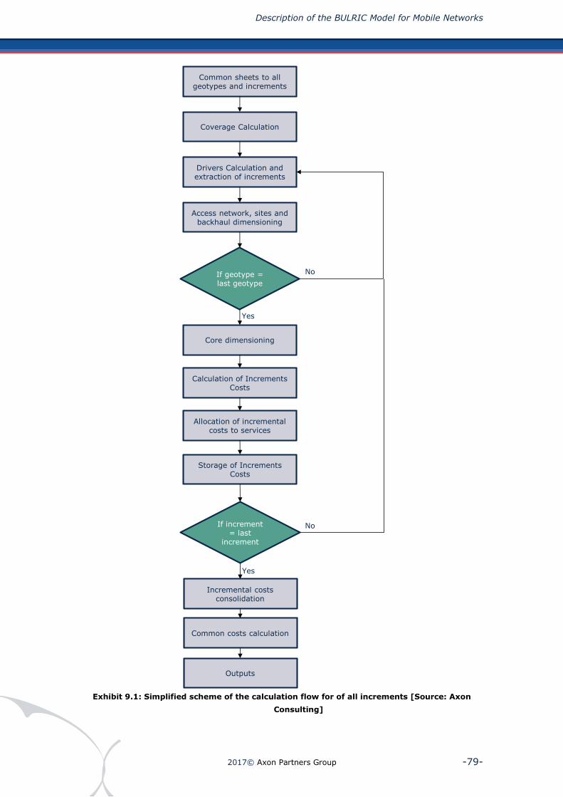
Description of the BULRIC Model for Mobile Networks
2017© Axon Partners Group -79-
Exhibit 9.1: Simplified scheme of the calculation flow for of all increments [Source: Axon
Consulting]
Common sheets to all geotypes and increments
Coverage Calculation
Drivers Calculation and extraction of increments
Access network, sites and backhaul dimensioning
If geotype = last geotype
Core dimensioning
Calculation of Increments Costs
Storage of Increments Costs
Incremental costs consolidation
Common costs calculation
If increment = last
increment
Yes
Yes
No
No
Allocation of incremental costs to services
Outputs

Description of the BULRIC Model for Mobile Networks
2017© Axon Partners Group -80-
Please note that in sheet ‘5E CALC DRIVERS CONSOL’, the services included in the
increment considered at a particular time are subtracted, which represents the step
‘Drivers Calculation and Extraction of Increments’ in the chart, shown above. After
subtracting this traffic, the model is run following the steps described in this
document.
After finishing the execution of an increment, the increment’s annual costs (defined
as the difference between the total costs, previously obtained, and costs obtained by
removing the increment’s traffic) are allocated to services12 and saved in sheet ‘11E
MAC SERVICES COST’. This step represents the ‘Storage of Increments Costs’ in the
preceding chart.
It should be stressed that, for incremental costs, the full model must be run as many
times as the number of increments, plus one, to obtain the total cost13.
9.3. Common cost calculation
Once each of the increments defined are run, the incremental costs per services are
consolidated and common network costs are calculated as the difference between the
total cost base obtained under the LRIC standard and the total incremental costs
extracted, as explained in the following formula:
𝐶𝑜𝑚𝑚𝑜𝑛 𝐶𝑜𝑠𝑡𝑠14 = 𝐹𝐴𝐶 − 𝑃𝑢𝑟𝑒𝐿𝑅𝐼𝐶(1) − 𝑃𝑢𝑟𝑒𝐿𝑅𝐼𝐶(2) − 𝑃𝑢𝑟𝑒𝐿𝑅𝐼𝐶(3)
Aligned with the methodology, the common costs are allocated to services though
routing factors (effective capacity approach).
Once the services’ common costs are calculated, the LRIC+ methodology is calculated
using the following formula:
𝐿𝑅𝐼𝐶 + 𝐶𝑜𝑠𝑡 = 𝑃𝑢𝑟𝑒 𝐿𝑅𝐼𝐶 𝑐𝑜𝑠𝑡 + 𝐶𝑜𝑚𝑚𝑜𝑛 𝐶𝑜𝑠𝑡𝑠
12 This step considers the same methodology of using routing factors as employed for the allocation of costs under the FAC standard, described in section 9 of this document. 13 This loop is controlled by the Visual Basic macro that manages the execution flow of the model’s sheets. 14 The common costs represent the cost of the network needed to carry the traffic from any point to any other point in the Member State.

Description of the BULRIC Model for Mobile Networks
2017© Axon Partners Group -81-
10. Cost Overheads
As defined in the methodology and principles defined by the ECTEL, the OpEx related
network working capital should be calculated as a percentage of network OpEx
(overheads).
Based on the information available, the most suitable alternative found has been the
calculation of a percentage overhead over network costs, similarly to what is applied
for the working capital.
Based on this methodology, network OpEx working capital is calculated as follows:
Network OpEx working capital:
𝑁𝑒𝑡𝑤𝑜𝑟𝑘 𝑂𝑝𝑒𝑥 𝑊𝑜𝑟𝑘𝑖𝑛𝑔 𝐶𝑎𝑝𝑖𝑡𝑎𝑙 = 𝑊𝐶𝑂𝑣𝑒𝑟ℎ𝑒𝑎𝑑 ∗ 𝑁𝑒𝑡𝑤𝑜𝑟𝑘 𝑂𝑝𝐸𝑥
Please note that the overhead percentages are calculated based on the operator’s
overall financial statements consistent with the formula above.

Description of the BULRIC Model for Mobile Networks
2017© Axon Partners Group -82-
Annex A. Detailed Geographical
Analysis by Member State
This annex presents the geographical analysis results for each member state.
A.1. Geographical analysis for access network
The following information represents the geographical information results, as used
for dimensioning access nodes and the backhaul network.
In accordance with the consideration mention in section 5.2.4, the population centres
of all the countries have been aggregated into geotypes, as is shown in the exhibits
below.
Exhibit A 1. Population centre geotypes for Dominica [Source: Axon Consulting]
Urban Dense
Urban
Suburban Dense
Suburban
Rural Mountainous
Rural Non Mountainous
Rural Spread Mountainous
Rural Spread Non Mountainous
Access Sites Samples
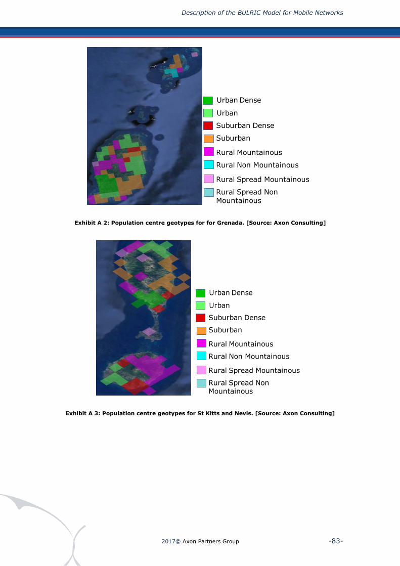
Description of the BULRIC Model for Mobile Networks
2017© Axon Partners Group -83-
Exhibit A 2: Population centre geotypes for for Grenada. [Source: Axon Consulting]
Exhibit A 3: Population centre geotypes for St Kitts and Nevis. [Source: Axon Consulting]
Urban Dense
Urban
Suburban Dense
Suburban
Rural Mountainous
Rural Non Mountainous
Rural Spread Mountainous
Rural Spread Non Mountainous
Access Sites Samples
Urban Dense
Urban
Suburban Dense
Suburban
Rural Mountainous
Rural Non Mountainous
Rural Spread Mountainous
Rural Spread Non Mountainous
Access Sites Samples

Description of the BULRIC Model for Mobile Networks
2017© Axon Partners Group -84-
Exhibit A 4: Population centre geotypes for St Lucia [Source: Axon Consulting]
Exhibit A 5: Population centre geotypes for St Vincent and the Grenadines. [Source: Axon
Consulting]
The following tables show the main characteristics of the geotypes defined in the
model for member states.
Urban Dense
Urban
Suburban Dense
Suburban
Rural Mountainous
Rural Non Mountainous
Rural Spread Mountainous
Rural Spread Non Mountainous
Access Sites Samples
Urban Dense
Urban
Suburban Dense
Suburban
Rural Mountainous
Rural Non Mountainous
Rural Spread Mountainous
Rural Spread Non Mountainous
Access Sites Samples

Description of the BULRIC Model for Mobile Networks
2017© Axon Partners Group -85-
Geotype Area Population Population
centres
URBAN_DENSE 55 31,635 21
URBAN - - -
SUBURBAN_DENSE 35 10,710 9
SUBURBAN 39 7,888 11
RURAL_SPREAD-NON MOUNTAINOUS
- - -
RURAL_SPREAD-MOUNTAINOUS 82 9,897 19
RURAL-MOUNTAINOUS 102 12,550 46
RURAL-NON MOUNTAINOUS - - -
TOTAL 314 72,680 106
Table A 1. Information regarding the grouping of samples into geotypes for Dominica
[Source: Axon Consulting]
Geotype Area Population Population
centres
URBAN_DENSE 48 25,757 48
URBAN 96 36,632 90
SUBURBAN_DENSE 12 3,365 12
SUBURBAN 128 28,981 86
RURAL_SPREAD-NON MOUNTAINOUS
- - -
RURAL_SPREAD-MOUNTAINOUS 8 335 2
RURAL-MOUNTAINOUS 68 9,941 35
RURAL-NON MOUNTAINOUS 16 1,814 4
TOTAL 375 106,825 277
Table A 2. Information regarding the grouping of samples into geotypes for Grenada [Source:
Axon Consulting]
Geotype Area Population Population
centres
URBAN_DENSE 24 19,584 19
URBAN 40 11,694 21
SUBURBAN_DENSE 40 5,328 28
SUBURBAN 60 10,395 21
RURAL_SPREAD-NON MOUNTAINOUS
- - -
RURAL_SPREAD-MOUNTAINOUS 20 1,756 3
RURAL-MOUNTAINOUS 76 6,815 28
RURAL-NON MOUNTAINOUS - - -
TOTAL 260 55,572 120
Table A 3. Information regarding the grouping of samples into geotypes for St Kitts and Nevis
[Source: Axon Consulting]

Description of the BULRIC Model for Mobile Networks
2017© Axon Partners Group -86-
Geotype Area Population Population
centres
URBAN_DENSE 120 101,933 80
URBAN 84 24,870 35
SUBURBAN_DENSE 92 27,994 49
SUBURBAN 88 20,037 38
RURAL_SPREAD-NON MOUNTAINOUS
- - -
RURAL_SPREAD-MOUNTAINOUS 8 635 2
RURAL-MOUNTAINOUS 60 9,529 23
RURAL-NON MOUNTAINOUS - - -
TOTAL 452 184,999 227
Table A 4. Information regarding the grouping of samples into geotypes for St Lucia [Source:
Axon Consulting]
Geotype Area Population Population
centres
URBAN_DENSE 146 94,787 46
URBAN 8 15 1
SUBURBAN_DENSE 12 2,853 4
SUBURBAN 36 7,733 13
RURAL_SPREAD-NON MOUNTAINOUS
12 227 2
RURAL_SPREAD-MOUNTAINOUS 20 1,123 5
RURAL-MOUNTAINOUS 32 1,501 10
RURAL-NON MOUNTAINOUS 8 1,222 3
TOTAL 273 109,462 84
Table A 5. Information regarding the grouping of samples into geotypes for St Vincent and the
Grenadines [Source: Axon Consulting]
A.2. Geographical analysis for core network
The following exhibits present the topology of the core network, traffic aggregation
nodes and backbone links defined for the reference operator.

Description of the BULRIC Model for Mobile Networks
2017© Axon Partners Group -87-
Exhibit A 6: Topology of the core network for Dominica. [Source: Axon Consulting]
Core Node
Backbone Node
Backbone Link

Description of the BULRIC Model for Mobile Networks
2017© Axon Partners Group -88-
Exhibit A 7: Topology of the core network for Grenada. [Source: Axon Consulting]
Exhibit A 8: Topology of the core network for St Kitts and Nevis. [Source: Axon Consulting]
Core Node
Backbone Node
Backbone Link
Core Node
Backbone Node
Backbone Link
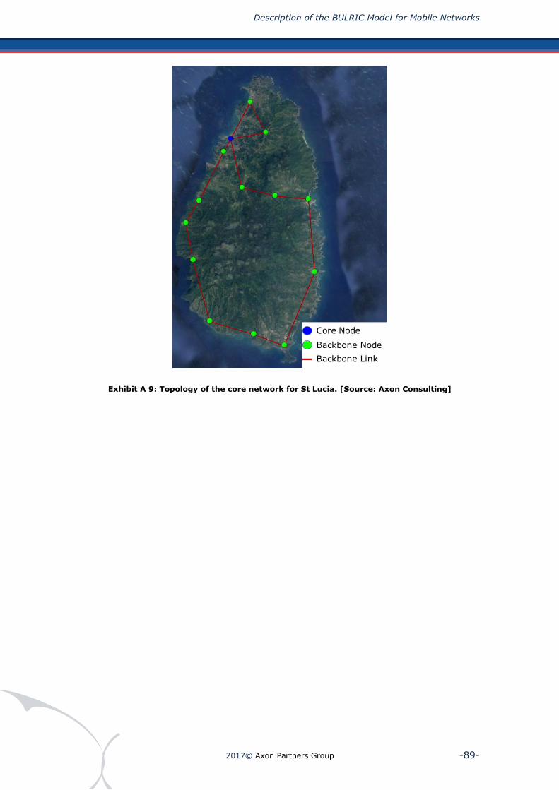
Description of the BULRIC Model for Mobile Networks
2017© Axon Partners Group -89-
Exhibit A 9: Topology of the core network for St Lucia. [Source: Axon Consulting]
Core Node
Backbone Node
Backbone Link
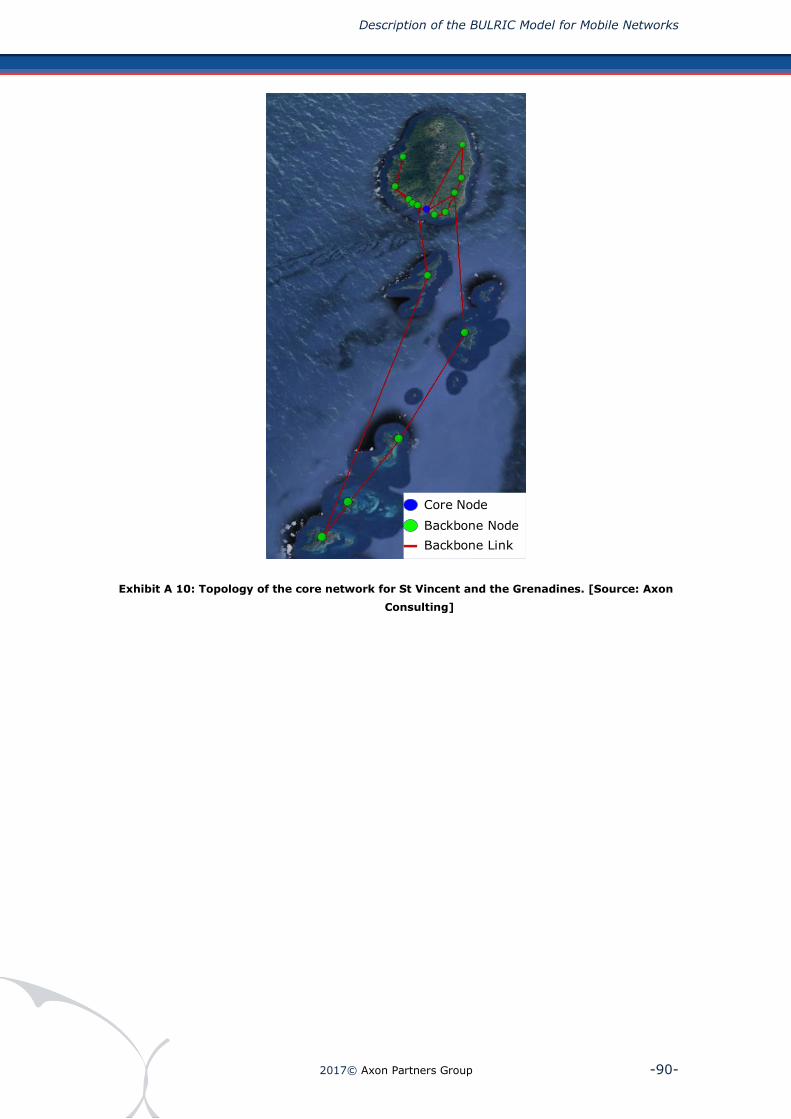
Description of the BULRIC Model for Mobile Networks
2017© Axon Partners Group -90-
Exhibit A 10: Topology of the core network for St Vincent and the Grenadines. [Source: Axon
Consulting]
Core Node
Backbone Node
Backbone Link