AD-AlGA 477 ANALYTIC SERVICES INC ARLINGTON VA F/6 22/3THE PREDICTION OF SATELLITE EPHEMERIS ERRORS AS THET RESULT FRO--ETC(U)A UG al B E SIMMONS F4962G-77-C-GGZS

UNCLASSIFIED ANSER SPDNAIV- NiL

2 ffffffffffffEhEEEEEEEEmhE

EEmmhEEEEEEEEEE

11111.25 1.4 11111J.6

NAKR0(O N i ,(t UJflLN I i I HA

f4A l *~,, *

- '4CA

Ilop

jgTk' 3*jr

~ 2~ AD

Ali;

lo' t

SPACE DIVISION NOTESpDN G"-

THE PREDICTION OFSATELLITE EPHEMERIS ERRORS

AS THEY RESULT FROMSURV EILLANCE -SYSTEM MEASUREMENT ERRORS

August 1981

Dr. B. E. Simmons

Approved byP. A. Adler, Division Manager

SApproved for public releae.distributo unmied

anser &aof[w a.A~wV"23=

ABSTRACT

This report derives equations predicting satellite

ephemeris error as a function of measurement errors of

space-surveillance sensors. These equations lend them-

selves to rapid computation with modest computer re-

sources. They are applicable over prediction times such

that measurement errors, rather than uncertainties of

atmospheric drag and of Earth shape, dominate in producing

ephemeris error. This report describes the specialization

of these equations underlying the ANSER computer program,

SEEM (Satellite Ephemeris Error Model). The intent is

that this report be of utility to users of SEEM for in-

terpretive purposes, and to computer programmers who

may need a mathematical point of departure for limited

generalization of SEEM.

*M & SO A- o..

i ii

ACKNOWLEDGMENTS

The author is extremely grateful to the following col-

leagues at ANSER for their valuable assistance and sugges-

tions relative to this report: Mr. Robert C. Morehead,

Dr. Lynne C. Wright, Dr. Charles E. Dutton, Mr. John N.

Kirkham, Dr. Arnold A. Shostak, Mr. Charles L. Smith, Jr.,

and Dr. Truett L. Smith.

To Ms. Teresa A. Huffine go special thanks for her

high standards of excellence and her patience in typing

this report with its myriad of equations.

Finally, the author is indebted to Maj Howard F. Steers,

AF/RDSD, for his sponsorship; and, for their continuing

interest and encouragement, to Maj Dennis F. Eagan and

Maj Leonard C. Tatum, AF/XOORS; to Mr. Max H. Lane, Head-

quarters ADCOM/DOG; and to Mr. Paul A. Adler, Deputy Manager,

Space Division, ANSER.

Dr. Bowen Eugene SimmonsAugust 1981

vSAM-NO MAS

PMSO31N~

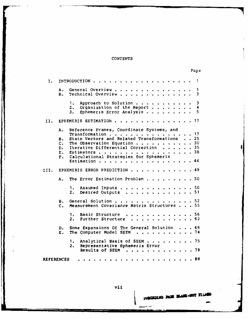
CONTENTS

Page

I. INTRODUCTION ..................... 1

A. General Overview ............... 1B. Technical Overview ....... .............. 3

1. Approach to Solution .... .......... . 32. Organization of the Report .... ........ 43. Ephemeris Error Analysis .... ......... 5

II. EPHEMERIS ESTIMATION . . ............... 17

A. Reference Frames, Coordinate Systems, andTransformation ... .......... ... ... 17

B. State Vectors and Related Transformations . . 25C. The Observation Equation.. . . ... ....... .30D. Iterative Differential Correction . . . . .. 35E. Estimators . . ......... .. .... . 38F. Calculational Strategies for Ephemeris

Estimation . . .................. 44

III. EPHEMERIS ERROR PREDICTION . . . . . . ...... 49

A. The Error Estimation Problem ... ......... .50

1. Assumed Inputs . . . ........... 502. Desired Outputs . . . . . ....... 51

B. General Solution. ...... ............. .52C. Measurement Covariance Matrix Structures . . . 55

1. Basic Structure ............. 562. Further Structure ............ 62

D. Some Expansions Of The General Solution . . . 69E. The Computer Model SEEM . . .......... 74

1. Analytical Basis of SEEM . . . . . .... 752. Representative Ephemeris Error

Results of SEEM . . . . . . . . . . . . . 79

REFERENCES . . . . . . . . . . . . . . . . . . . . . 88

vii

FW-e

CONTENTS-Continued

Page

APPENDIX A-Covariance Matrices:Definition and Properties .. ......... . A-I

1. Definition and General Properties . . . A-22. Properties When The Density Function

Is Normal ............... A-8

BIBLIOGRAPHY ............... A-1

APPENDIX B-Propagation Error Matrix . . . . . . . . . B-i

1. The Propagation Error Matrix Problem . B-22. Solution Summary and Results . . . . . B-43. Derivation of Partial Derivatives . . . B-6

REFERENCES ................ B-12

APPENDIX C-Inversion of a Matrix ... ........... . C-i

APPENDIX D-Primary Distribution List .. ......... . D-i

Viii

FIGURES

Figute Page

1 Relationship of Inertial (xyz) toTopocentric (x'y'z') Reference Frames . . . 19

2 Altazimuth Coordinates in the TopocentricReference Frames ................. .... 19

3 Ephemeris Errors: Single-Pass, "Nominal"Measurement Errors ................ ... 82

4 Ephemeris Errors: Single-Pass with ZeroResidual-Bias Errors ............... ... 83

5 Ephemeris Error: Two Passes, Quarter-Revolution Spacing ................ ... 84

6 Ephemeris Error: Two Passes, Half-Revolution Spacing ..... ............. 85

TABLES

Tabte Page

1 Transformation Quantities . . . . . . . . . 21

2 Transformation Matrices: Earth-SurfaceAltazimuth Coordinates .............. . 23

3 The Matrix *ji (Special Case) ...... 28

4 Representative (4, M) Pairs ........ . 32

5 Some Structure Combinations For C and D . . 72

6 State-Vector Error Matrices For StructureOf Table 5. . . . . . . . . . . . . . . . 73

7 "Nominal" Standard Deviations ofMeasurement . . . . . . . . . . . . . . . 81

8 Inputs for SEEM Examples . . . . . . . . 81

A-I Some Useful P Values. . . . . . . . . . . A-15

B-1 Partial Derivatives . . . . . . . . . . . 9-7

ix

. . . . . . . . . .. .... .. . . . ... ... . A

I. INTRODUCTION

A. General Overview

Earth-satellite ephemeris estimation (i.e., positionprediction) is fundamental to many space-related operations.

Measurements by friendly space-surveillance sensors are

computer processed to yield necessary ephemerides. Eachephemeris thus provided has some characteristic accuracy.

The prediction of ephemeris error is also important,both operationally and in the planning of space surveil-

lance systems and of data reduction procedures.

The problem addressed here is the mathematical predic-tion of ephemeris error, as it results from measurement

error alone. The results are valid under conditions whereone may validly ignore uncerta~inties of atmospheric drag andof Earth shape. A major requirement was that resulting equa-

tions be suitable for computer programming to obtain rapid

calculations with modest computer resources.

This report presents a detailed, general parametric solu-tion to the above problem. This report gives, in particular,

the somewhat speciali'zed form of that solution, which is the

basis of the new ANSER computer program, SEEM (Satellite

Ephemeris Error Model).*

SEEM demonstrates, with a time-shared HIS-635 computer,the requisite programming suitability of the mathematical

results herein. Reference 1 describes successful use of

*A FORTRAN program, written by the author of this report,as yet unpublished.

1A L W WTyj4

SEEM empirically to investigate conditions of its validity

for ephemeris error prediction vis-a-vis Earth-based radar

sensors.*

This report is directed, first, to users of SEEM who

may wish to understand its fundamental interpretation. It

is also directed to computer programmers who may wish tomodify certain specializations of the current version of

SEEM and need a mathematical point of departure. The in-

tent is that material here be accessible to engineers and

scientists who do not necessarily specialize in either

statistics or astrodynamics.

Thus, this report is semi-tutorial in style, and is

derivationally self-contained to the extent practical. Some

original mathematical developments are included and appro-

priately noted.

B. Technical Overview

The purpose of this section is to provide not only an

overview of report organization, but also a substantive dis-

cussion of ephemeris error estimation sufficient (I) for

* A summary of established SEEM applicability is as follows.

The model validly accommodates drag forces for satellitealtitudes above about 180 km, over time intervals--encom-passing both sensor measurements and the prediction times-of up to at least 9 hours. The model validly accom-modates noncentral-forces gravitational fields for low-altitude satellite passes by as many as three Earth-basedradars, over somewhat longer measurement-and-predictiontime intervals. Assumptions here are (1) current capa-bility for predicting drag forces; (2) current under-standing of geoid and other gravitational perturbations;and (3) no radical radar accuracy improvements beyondtoday's state-of-the-art.

2

routine interpretation of SEEM inputs and outputs, and (2)

for appreciation of options for limited generalization of

SEEM.

Three subsections follow. The first gives the overall

technical approach. The second overviews report organiza-

tion, and in particular that of Chapter II. The third

discusses substantively Chapter III, the heart of the report.

1. Approach to Solution

The overall approach to solution o: the stated problem

is to ignore drag and geoid uncertainties by estimating

ephemeris errors under the Keplerian (central-force-field)

approximation. The rationale for this approach is that the

distance of a "Keplerian" satellite from a Keplerian-estimated

position should approximate the distance of a "real-world"

satellite from a position estimated via perturbation theory,

provided that calculational treatment of perturbations is

exact.

The cited investigations of Reference 1 appear to con-

firm the validity of the Keplerian approximation for the

problem at hand.

The specific analytical approach of this report is

parametric, utilizing standard linear-algebra procedures

in a covariance-matrix formulation.

2. Organization of the Report

This report constitutes three chapters, plus four ap-

pendices. The non-statistician reader may wish to read

Appendix A before proceeding to Chapter II. Appendix A is

a purely tutorial review of covariance matrix theory.

3

Cnapter II reviews the linear-algebra theory by which

one may estimate ephemerides-in a Keplerian universe-

from sensor measurements. This chapter serves also to de-

velop the notation used later on. The theory of Chapter 11

accommodates a variety of sensor types, sensor basing both

terrestrial and on satellites, and a variety of "unbiased

statistical estimators."

Section II.A defines useful coordinate systems, and some

matrix transformations among finite and infinitesimal (error)

vectors in those systems. Section II.B, drawing upon Appen-

dix B, deals with transition matrices between astrodynamical

state vectors and between error vectors associated with those

states.

Section II.C derives the sensor "observation equation."

Section II.D treats the iterative differential correction

process, which transforms observations into an estimated

state vector corresponding to an arbitrary epoch (i.e., in-

stant in time). A subset of the components of this vector

constitutes an ephemeris estimate.

Section II.E discusses error minimization criteria and

associated unbiased statistical estimators. Finally, Section

II.F outlines calculational shortcuts for (1) estimating

state vectors for many epochs, and (2) revising state-vector

estimates so as to exploit newly available measurement data.

The next subsection describes Chapter III both organiza-

tionally and substantively, and also defines the supporting

role of Appendix C.

4

3. Ephemeris Error Analysis

Chapter III deals with prediction of errors in ephemer-

ides that would be arrived at by the methods of Chapter II.*

This error analysis assumes perfect convergence of the iter-I ative differential correction process of ephemeris estimation.Thus, the limiting accuracy characteristics of a particular

ephemeris estimation process are amenable to assessment, even

without analyzing the practical convergence properties of tnat

process.

a. Inputs, Outputs, and General Solution

Section III.A defines in mathematical terms the as-

sumed inputs and desired outputs of the problem.

Key desired outputs are the standard deviations of

the components of satellite position error, for the time of

each ephemeris. These are to be expressed in a coordinate

system selected to make correlations among ephemeris error

components vanish. Further desired outputs are tne orien-

tation angles of that coordinate system, relative to a "UV4"

system defined as having the following axes at an instant

in time:

RADIAL - Up: geocenter toward satellite

"ALONG-TRACK" - A third axis orthogonal to the other

two axes, approximately along the sat-

ellite velocity vector (exact for cir-

cular orbits)

*Actual estimation of ephemerides is unnecessary to esti-mate their errors.

5

CROSS-TRACK - Normal to the orbital plane, di-

rected along the satellite angular

momentum vector.

The above standard deviations and orientation angles

have a particularly simple physical interpretation if, in

addition to the input assumptions listed below, the probabil-

ity distributions of the measurement errors are of multivariate

normal (Gaussian) form. Then (see Appendix A) one may inter-

pret the standard deviations as the principal nalf-axial di-

mensions of a "10" ellipsoidal confidence volume, oriented

along the axes of the rotated coordinate system. One may

interpret the ellipsoid as centered either at the true ephein-

eris, expressive of a level of confidence that the estimated

ephemeris will fall within the ellipsoid; or as centered on

the estimated ephemeris, expressive of a level of confidence

that the true ephemeris will fall within the ellipsoid.

The level of confidence of a 10 ellipsoid of satel-

lite position is about 20 percent. For many interpreta-

tive purposes, a 3a ellipsoid (i.e., having triple the dimen-

sions of the la ellipsoid) is more useful, providing a con-

fidence level of 61 percent.

Assumed inputs are (1) the *true" orbit parameters

of the satellite; (2) sensor types (measuring any subset

of the quantities: range, two angles, and their respec-

tive rates) and locations (sensors may be fixed or may move

on or above the Earth's surface); (3) sensor envelopes of

geometric coverage (range and angle extrema); (4) the as-

sumption that sensor measurements are "unbiased"; (5) 'true"

statistical parameters of measurement error, in the form of

6

a covariance matrix D covering all sensor measurements made;

(6) the covariance matrix C-some approximation to D-

characterizing the "estimator" via which actual estimation

of ephemerides would proceed; and (7) the instants in time

corresponding to the presumed ephemerides whose accuracy is

in question.

There are still further assumed inputs, whicn, how-

ever, derive calculationally from above inputs (1), (2), and

(3). These further inputs are "ideal" (error-free) sensor

observation data of the target satellite. A "driver" program

to generate these data preexisted SEEM at ANSER.* This re-

port does not give the full mathematical basis of such a

driver program, although Sections II.A and II.B do provide

many of the necessary transformations.

Regarding inputs (5) and (6) above, the matrices D

and C typically contain >106 elements each. Apparently,

their general parametric specification poses a practical

difficulty. Actually, in the case of C, this difficulty

must in some sense be resolvable relative to any practica:

procedure for ephemeris estimation, since any such proce-

dure involves specification of C (see ensuing discussion

of Section III.C).

Section III.B gives the general solution equations

for Keplerian ephemeris error prediction. These equations

* A multipurpose Keplerian program, thus far unpublished.It utilizes a modified Earth rotation rate, therebycorrecting to first order for the drift of the satelliteorbital plane due to the Earth's equatorial bulge.

7

provide desired outputs as a function of assumed inputs.

These equations appear to present a further practical dif-

ficulty, in that they require extraction of the inverse of

the large matrix C.*

As before, this difficulty must actually be resolv-

able for error prediction relative to any practical proce-

dure for ephemeris estimation, since extraction of C-1 is

necessary there also. However, this difficulty is not nec-

essarily resolvable relative to *ideal" ephemeris estimation,

for which one must take C - D.

b. Detailing of the General Solution

Section III.C presents candidate representations of

D that resolve the specificational, and in one case also the

inversion, difficulties identified above. These represen-

tations serve as a point of departure for selection of C

representations applicable to ephemeris estimation and, con-

comitantly, to ephemeris error prediction. The two subsec-

tions of Section III.C warrant detailed discussion here.

Subsection III.C.1 begins by assuming that in the

OrealO Keplerian world, raw measurement data are prepro-

cessed at each sensor for each pass as follows, for entry

into the ephemeris estimation process.

Repeatedly, raw data accumulated over an interval of

a few seconds are suitably averaged, such that the averaged

results correspond to the instant at the center of the ob-

servation interval. Known corrections for systematic error

*Practical, not theoretical, invertibility of C is at issuehere. Theoretical existence of C-1 follows fromt the defi-nition of C as a covariance matrix, with the stipulationthat 'perfect" sensors (i.e., having any zero standarddeviation of measurement error) are not allowed.

(e.g., sensor calibration corrections) are then applied tothe averaged data to form a single "observation vector." If

the sensor happens to be a doppler radar, for example, ob-

servation components would be range, two angles, and range

rate. At the end of the pass, the collection of all obser-vation vectors is then fed into the ephemeris estimation

process. Subsection III.C.1 defines D to be the "true"

covariance matrix of the errors of all observation vec-

tors, over all passes and sensors.

This subsection then treats the errors of each ob-servation vector as the sum of "noise errors" and "residual

bias errors," the latter accounting for all residual system-

atic errors in the observation. By assumption, noise errorsmay be correlated with each other within an observation, but

not from observation to observation. By further assumption,

the noise errors are uncorrelated with residual bias errors,

within an observation and from observation to observation.In order to exclude "perfect" sensors, all noise-error stand-

ard deviations must be nonvanishing, however small. In order

to ensure "unbiased" measurements, it is sufficient to assume

that both noise-error and residual-bias error probability

distributions are symmetric about zero.

The effect of this decomposition upon D is to renderit the sum of a "noise matrix" and a "residual bias matrix."

Of these, the noise matrix is block diagonal, each block

being the covariance matrix of a single observation and of

dimensionality at most 6 x 6. If the noise errors of an

observation happen to be uncorrelated among themselves, the

corresponding block will be diagonal.

9

The residual bias matrix may, however, be relatively

complicated, with widespread off-diagonal terms representing

long-term correlations among residual-bias errors. Subsec-

tion II1.C.1 takes a first step toward simplifying this ma-

trix by assuming zero correlation among residual-bias errors

of different sensors. Thus, with appropriate organization

of D, the residual-bias matrix becomes block diagonal, each

block corresponding to all the passes by a particular

sensor.

Subsection III.C.1 concludes by developing a detailed

parametric representation for the noise and residual-bias

matrices, structured as just described. Parameters comprise

various error standard deviations and correlation coefficien-

cies, with general functional dependencies upon satellite

position relative to the sensor.

Thus, Subsection III.C.1 provides D structures that

are physically realistic for a wide variety of sensing con-

ditions. It also provides a parametric formalism lending

itself to practical specification of D as an input to ephem-

eris error prediction. However, because of the large blocks

of elements within the residual bias matrix, the structuring

of Subsection III.C.1 is not generally sufficient to provide

practical invertibilty of D. Hence, this D-structure does

not generally permit "ideal" ephemeris estimation with C - D.

The objective of Subsection III.C.2 is to furtner

structure the residual-bias matrix so as to arrive at an

easily invertible D, yet accord with physical reality for at

least some measurement circumstances.

10

Subsection III.C.2 assumes, for any given sensor,

that the residual bias errors do not change appreciably

over a pass, or alternatively over several passes closely

spaced in time (a "pass multiplet").* This subsection

further assumes that residual biases change significantly

between pass multiplets (but their standard deviations do

not change) such that residual-bias correlations vanish

between multiplets.

Thus, each sensor block of the residual bias matrix

decomposes into a set of small blocks, each corresponding to

a pass multiplet for that sensor. Each multiplet block con-

stitutes a set of partitions-corresponding to individual

observation vectors-that are identical over the entire

block.

With the aid of a derivation detailed in Appendix C,

Subsection III.C.2 infers and then proves the validity of a

closed-form equation yielding D-1 as a function (1) of the

partitions of the residual bias matrix and (2) of the in-

verses of the partitions of the noise matrix. (As mentioned

earlier, these partitions are of maximum 6 x 6 dimensionality.)

Hence, except for matrix multiplications involving the parti-

tions of the residual-bias matrix, this equation reduces the

complexity of extracting D- 1 (as structured) to that of

calculating the inverse of the noise matrix alone.t

* Note the implication that residual-bias error is insensi-tive to satellite position relative to the sensor. Thisassumption may be inappropriate, for example, if it shouldhappen that atmospheric-refraction uncertainties becomelarge at angles near the horizon.

t This equation may be unique to this report. However, aliterature search was not feasible within the scope ofthis analysis effort.

11

To summarize, Section III.C provides various candi-

date D-structures, including structures intermediate to those

just described, for use in detailed expansion of the general

error-prediction equations in Section III.B.

Section III.D continues first by introducing two

broad classes of C-structures as approximations to D, and

some gradations among them. Section III.D then explicitly

details the general solution equations for seven combinations

of D-structures and C-structures.

The first class of C-structures constitutes those

congruent to the noise matrix of D, i.e., those wnich are

block diagonal, elsewhere with zeroes for every element

representing correlations from one observation to another.

These structures are readily invertible and give rise to what

is sometimes referred to as 'weighted-least-squares" (WLS)

ephemeris estimation. WLS estimation ignores all correla-

tions from one observation to another.

"Simple" WLS estimation, a special case, in addition

ignores all correlations among measured quantities within an

observation, i.e., it uses a C-structure that is strictly

diagonal. This is equivalent to the classical estimation

method of Gauss, and produces an optimum fit of the estimated

orbit to actuaZ sensor measurements (see Section II.E).

The second class of C-structures consists of those

allowing nonvanishing elements that represent correlations

among observations. These structures generally incur practi-

cal difficulties of inversion, and their use is not ordinarily

12

attempted in practice. The special case when actually C = D

gives rise to "minimum variance" estimation and produces-if

calculationally feasible-an optimum fit of the estimated

orbit to the true orbit.

Because of its ready invertibility, the "pass-multipleth

D-structure of Subsection III.C.2 offers the opportunity for

minimum variance e!timation when (1) that structure is valid,

and (2) parameters of measurement error are known with suf-

ficient accuracy that . becomes D.

Sectic-n 17 provides detailed expansions of the

general error prediction equation for C-structures that are

congruent to eac! of the D-structures of Section III.C, and

in addition for the WLS C-structure, which is congruent to

the noise-matrix of them all. All C-structures are distinct

from the D-structures, however, in that their parametric

values may be different-their parametric sets may even

be different for the same congruence constraint.

As the various expansions reveal, the amount of

feasible detailing of solutions is quite limited, except

for those C-structures whose inverses can be extracted

analytically. Those are the WLS C-structure and the "pass

multiplet" C-structure. These two expansion cases comprise

the point of departure for the specializations of SEEM.

c. The Mathematical Basis of SEEM

Section III.E, the final section of the final chap-

ter of the report, deals with SEEM. Of the two subsections,

III.E.2 presents and discusses numeric examples of SEEM out-

puts. That subsection requires no further discussion here.

Subsection III.E.1 gives the analytical specializations of

SEEM.

13

As input, SEEM accommodates only radars, and specifi-

cally only those that operate in "altazimuth" coordinates:

azimuth, elevation, and range.

One may, however, input a telescope-type sensor by a

strategem, i.e., by assigning a very large value to the range

measurement error. Thereby, one assigns a low statistical

weight to range measurements.

One may also (to some approximation) input other

range-and-two-angle coordinates, e.g., angles relative to

the boresight of a phased-array radar, by (1) in the driver

program, converting to altazimuth coordinates for the "ideal"

observation calculations; (2) in the driver program, finding

a geometrical coverage volume in altazimuth coordinates that

approximates the true coverage volume; and (3) assigning angle

errors to their nearest geometric angle analogs in azimuth and

elevation.

SEEM allows correlations only among errors of a given

measurement component-e.g., range-elevation error corre-

lations are not allowed. Thus, the observation blocks of

the D noise matrix are diagonal, as is each small partition

of the residual bias matrix.

Via the following additional assumptions, SEEM allows

specification of the error performance of each radar in terms

of six parameters, the first three being the (constant)

residual-bias standard deviations. The remaining three para-

meters are the noise errors, which are functionally dependent

upon satellite position in the radar field of view as follows:

(1) The standard deviation of azimuthal noise error

is proportional to 1/cos h, where h is elevation

angle (accounting for increasing indeterminacy

14

of azimuth measurements at elevation angles

approaching the zenith). The constant of pro-

portionality is hence the azimuthal standard

deviation at 0* elevation.

(2) The standard deviation of elevation noise error

is constant, not a function of azimuth, eleva-

tion, or range.

(3) The standard deviation of range noise error is

constant, not a function of azimuth, elevation,

or range.

In the light of (3) above, the present version of

SEEM may be inappropriate for high-altitude satellites, where

maximum range is set by radar range performance rather than

by horizon-limited line-of-sight. (SEEM validation did not

include satellite altitudes above approximately 1,000 km.)

SEEM defines all pass multiplets as containing just one pass.

Thus, the residual bias matrix of D-and hence also D itself-

is block diagonal in one-pass blocks.

SEEM provides two choices of C for characterizing

the ephemeris estimation process. In the "minimum variance"

choice, C = D. In the "least squares" choice, C is set equal

to the noise matrix of D. (SEEM validation was conducted

only for the least-squares choice.)

SEEM ephemeris error component standard deviations

are specified in UVW coordinates only, and do not include

correlation coefficients that may not vanish in those coor-

dinates. A further output, the standard deviation of the

resultant error vector is invariant with respect to

coordinate-system selection. Hence, the UVW resultant

error is correct even without coordinate rotation.

15

Empirical results with SEEM indicate that in fact

the error ellipsoid does align itself with the UVW axes

soon-in prediction time-after the most recent pass

(see Subsection III.E). This alignment is due primarily to

the effect of period uncertainty, which makes the along-

track error ordinarily large compared to radial and cross-

track errors.

16

t

II. EPHEMERIS ESTIMATION

This section describes linear-algebra methodology for es-

timating satellite ephemerides from sensor observations, as-

suming a Keplerian (central-force field) universe. There is

no restriction as to selection of a particular statistical

estimator, except that it be "unbiased."

Most of the material here occurs-in one form or another-

in References 2 and 3. A first-order correction term to

the error transition matrix [i.e., *ji in Equation (26)]

does not appear in Reference 2, but is well known in esti-

mation theory. The explicit representation of the partial

derivatives of qji may well be new as developed in

Appendix B, but are available elsewhere in somewhat dif-

ferent form [see p. B-6, including footnote].

To the exten: practical, the notation here follows the

Herrick standards (Reference 3, AstrodynaiiaZ Terra-noZogy,

Notation and Usage (Appendix), pp. 477-511]. The major ex-

ception here is that lightface uppercase Roman letters repre-

sent various matrices rather than specialized astrodynamical

quantities.

A. Reference Frames, Coordinate Systems, and Transformations

Let the time to be the (arbitrary) initial epoch of the

analysis. Referring to Figure 1, define a righthanded

Cartesian reference frame with positive z-axis through the

Earth's North Pole, and positive x-axis intersecting the

Greenwich meridian as it happens to lie at to.

* This x-axis choice promotes algebraic simplicity. Con-version of ensuing equations to a system with x-axispositive toward the vernal equinox is straightforward.

17

At time

t = t - t ( )0

let the satellite position be

r [j](2)and a sensor position be

[ T YT(3)LZ J

(One should not consider the sensor position as necessarily

on the Earth's surface, although it is so depicted in Figure 1

for ease of geometric interpretation.)

Again referring to Figure 1, define a topocentric

(sensor-centered) reference frame as righthanded Cartesian,

with positive z'-axis toward the zenith and positive x'-axis

toward the South point of the compass. In this frame let

the satellite position be

(4)[Ze

With these definitions,

r - + Ap (5)

19

FIGURE 1RELATIONSHIP OF INERTIAL (xyz) TO

TOPOCENTRIC (x'y'z') REFERENCE FRAMES

(North)z

Greenwich Meridian z

to / (South-Poini of Compass)

FIGURE 2ALTAZIMUTH COORDINATES

IN THE TOPOCENTRIC REFERENCE FRAMES

Satellite

X.

19

where A is a rotation matrix. Table 1 gives a representation

for rT and A in terms of sensor longitude A, latitude 4, and

geocenter distance rT.' These may be time-varying quantities.

Suppose now that one regards the components of p as func-

tions of an arbitrary set of curvilinear coordinates qj, q2, q3.

These will subsequently become the angle and range coordinates

characterizing operation of a given sensor. (Their particular

significance may, however, differ from sensor to sensor.) Let

r 1q2 ( J6)q 3

Differentiate Equation (5) with respect to time, obtaining

r= T+ip + A J4 (7)

where J is the Jacobian matrix for p as a function of q. Table

1 gives representations for A and J.

As an illustrative example, consider the case of a sensor

fixed at some position on the Earth's surface and designed to

operate in altazimuth coordinates. Following the notation

of Figure 2, one may write

* The representation of A is a standard result. One may de-rive it by taking products of elementary rotation matrices,which provide first, a rotation of the primed referenceframe about its y'-axis through the angle - (%/2 -4); andsecond, a rotatign about the (now) z-axis through theangle - (X + we t).

20

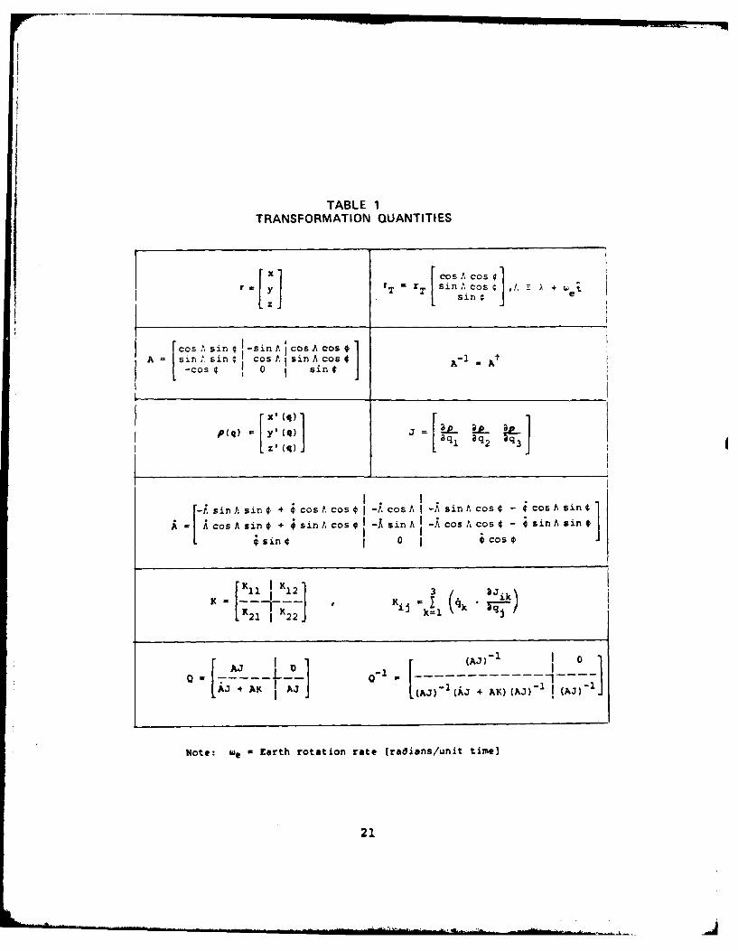
TABLE 1TRANSFORMATION QUANTITIES

rT sinP cos ,!, - . + esin € e

z

cos Asin 4 -sin A 1 CosA Cos$ -A = sin. sin 4 cos Li sinA cost A- 1 A%

-cos 4 1 0 sin €

O~q = jq = . .. EL.

az'(q) Eq1 aq 2 Oq3

snAsin 4+ 4cos A cos 4 ACos A I Asin A cos 4 - 4cos A sinCos i sin 4 + 4 sin A cos 4 sin A -l cos A cos 4 - sin A sin

[ sin€ I o 4cos

[rK1 K2 2 ] 3

X- K-2 = - (4k .. | ...

r i I- (AJ) 1 L 0

iJ A J (AJ)' (A3 + AK) (AJ) I(J

Note: we a Earth rotation rate (radians/unit time)

21

and arrive at the specialized transformation matrices of

Table 2.

Returning to the general case, introduce the composite

vectors

which will subsequently be useful. Equations (5) and (7)

provide a functional relationship between these vectors-

unfortunately, a nonlinear relationship since p(q) is nonlinear.

However, one can show that a fully linear relationship

does exist between the differentials of these vectors, of the

form

_69)

These vectors will represent errors at a particular instant,

so that in performing differentiations t is to be held constant.

To find Q, first differentiate Equation (5), regarding

both sensor position rT and the rotation matrix A as "known"

(i.e., error-free) and hence as constants. One obtains

6r - AJ6q (10)

Differentiating Equation (7),

r - £J6q + AK6q + AJ64 (11)

22

r -- - --

U _ _

0 0

0 C4 + 1 0oU II

X• 0. 0 .-

In m c au UU

t 0''4 U C

uI IW

Sin 0z CN 0

z << u 0 u o to -

10 - r

0, In IItI 1A c

IIcI 0 .c .-.4 ",4 U A Ut

4 ao aN 0 CL

z + x

CA..

,,'to H o

CC- < .1 .

0 U j

to m

< = u= "c r 8 "03C 5

x -4I t

S",' C .c goc +

Q"~ 0. 0 .m

cc 'A a

0

A uImm I A

FA Io n

> o II

VAI8

•L ,- 0

wIn

1A 0

23

AA.. ...

defining a new matrix K via the relation

AGJ4 E AK6q . (12)

Fror Equation (1) one can derive the representation for K

given in Table 1.

For the example of the Earth-based altazimuth-type sen-

sor, one can further derive the specialized representation

of K given in Table 2.

One can now find the general form of Q by comparing

Equations (9), (10), and (11). Table 1 gives the result

and also the form of Q-1 . One can prove the correct-

ness of Q-1 by taking the product QQ-1.

One further transformation will prove useful:

y" = L[Y (13)

Here L is the rotation matrix taking the inertial-frame (xyz)

representation of r into a U%"A representation (xuyazu) de-

fined as having the unit vector U(x"-axis) directed radially

outward from the Earth's center toward the satellite; the

unit vector W(z"-axis) directed along the angular momentum

vector, normal to the orbital plane; and hence the unit

vector V(y"-axis) approximately along-track in the direction

---exactly along-track for circular orbits.

To find L in terms of the inertial-frame (xyz) represen-

tation of r, begin by defining a quantity

| - r X (14)

24

(vector cross-product), proportional to the angular-momentum

vector. Clearly in the inertial-frame representation,

U = Y (15)

s (16)SZ

V 1 (5X[ X":SXri (5 X r) (17)

(s X r) Z

But the above nine unit-vector components are just the

direction cosines among the axes of the two reference frames,

and hence are the elements of the rotation matrix relating

the frames. That is,

L =[IV (18)

where notationally U t is the adjoint of U, etc. Hence, L

may be evaluated from Equations (12) - (15). Since L is a

rotation matrix,

1 L ( (19)

B. State Vectors and Related Transformations

One may represent the six parameters of a Keplerian orbit

(including the instantaneous position of the satellite in

that orbit) by the state vector

(20)

t t±J25

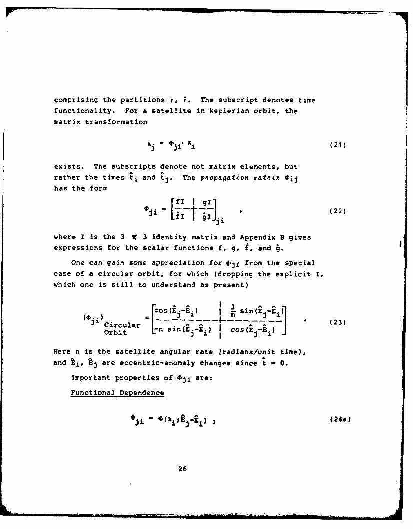
comprising the partitions r, r. The subscript denotes time

functionality. For a satellite in Keplerian orbit, the

matrix transformation

Ij f *ji. i (21)

exists. The subscripts denote not matrix elements, but

rather the times ti and tj. The p'opagation mat4ix ij

has the form

[f (22)

where I is the 3 W 3 identity matrix and Appendix B givesexpressions for the scalar functions f, g, f, and g. 1

One can gain some appreciation for 0ji from the special

case of a circular orbit, for which (dropping the explicit I,which one is still to understand as present)

s .- ~ in (E£ E£)( --j-i) =......(23)

Circular [-n sin(E.-Ei) I cos(E -Ei (Orbit j -

Here n is the satellite angular rate [radians/unit time],

and Ei, Ej are eccentric-anomaly changes since t - 0.

Important properties of 4ji are:

Functional Dependence

* j - *(ImE J- Ej) (24a)

26

.. . .

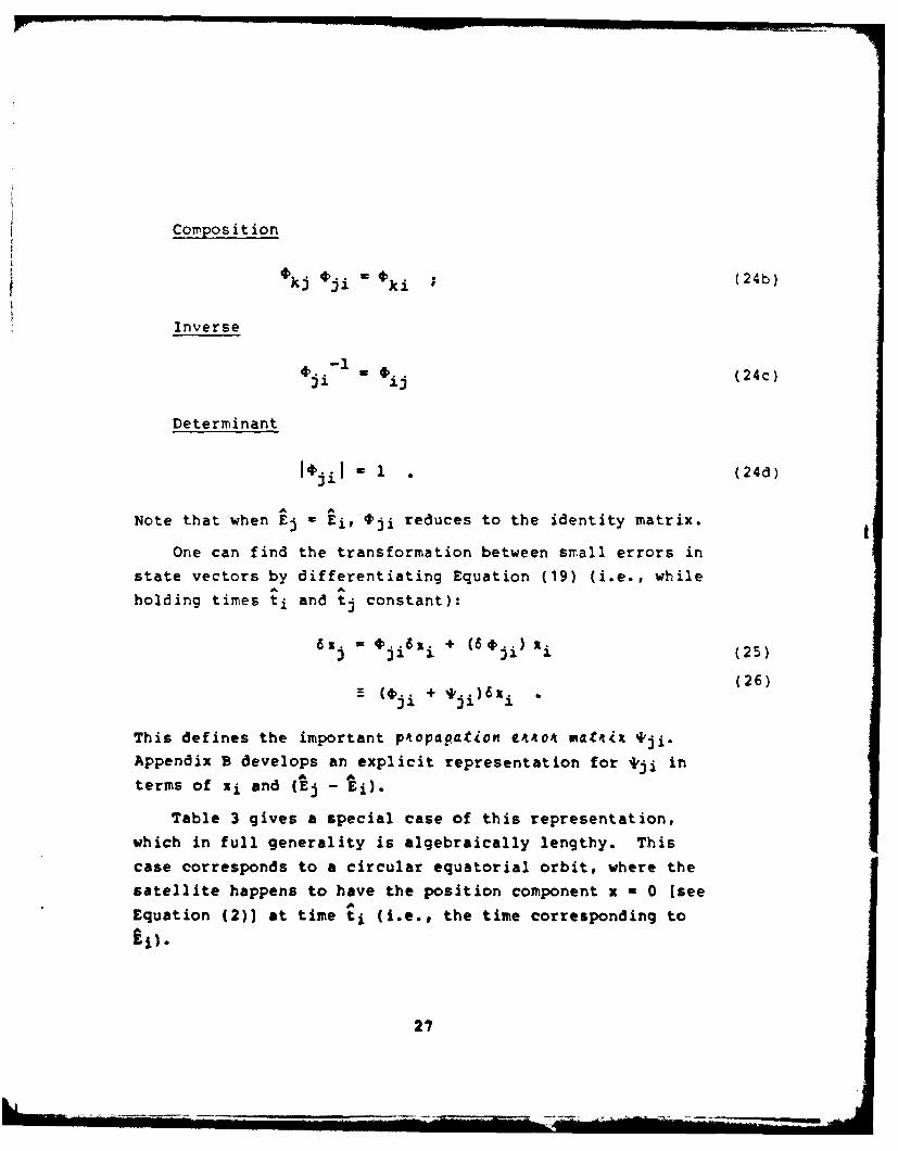
Composition

)kj )i (ki (24b)

Inverse

t ji4 =ij (24c)

Determinant

11jil - . (24d)

Note that when Ej - Ei, Oji reduces to the identity matrix.

One can find the transformation between small errors in

state vectors by differentiating Equation (19) (i.e., while

holding times ti and tj constant):

61. = tji6x (6 i) x i (25)

(26)=(4.. + * IE. )61i.I

This defines the important p'opapaion e444ao mdatx *ji-

Appendix B develops an explicit representation for *ji in

terms of x i and (Ej - ti).

Table 3 gives a special case of this representation,

which in full generality is algebraically lengthy. This

case corresponds to a circular equatorial orbit, where the

satellite happens to have the position component x - 0 [see

Equation (2)) at time t i (i.e., the time corresponding to

27

I I

on~ o

11i I I C Iwo

S II14 4w(h3 I I+~ 1-4 Ida*

r. 1 - CDui ~ ~I

CLUwU

-------o-~ I

I 00 4~I

V4 I c

I I -1 ~-~~F--------

I I cC4 I 0i'

I Ic I .1mI CW ai(1a ~.~to 5~U

u4J 0 5 -cw 0*

*4 1 ; 40 :dN '' I

-------

~ j 113 '~ (29

Important properties of *ji are:

Functional Dependence

= 4'(X. E-E.) ;(27)

Composition

(€) kj + +kj ) (ji + ji ) = ki + ki ( (28)

Inverse

+ + (29)

Determinant

1tji ** I 1, EI = Ei. (30a)

= lUbounded as j-il(30b)

increases without limit].

When Ej a Ei, ji = 0.

The inverse follows from the composition property by

setting k - i and using Equation (24a).

One may prove the composition property by differentiating

Equation (24b) as it operates upon xi

6 lmkil i ) - 6(4)kj4>jix i ) (31l (31)

Now apply the definitional Equation (26) first to the

lefthand side, and then repeatedly expand the righthand

side:

29

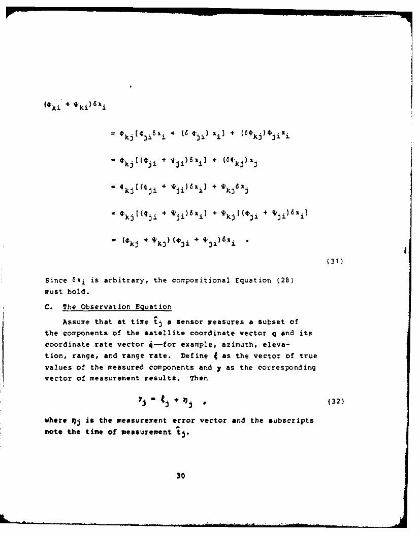
(4ki *ki ) 6 i

= ikj[#3ii + (+ tji) xi] + (6 kj) jiz i

t k[( ji + ji)6i] + (6 t kj)x

4 4kj[(4ji + *jil6xi] + *kj i

= 4k.I(4ji + .ji)6x] +4kj [()ji + qi )6x]

=( kj + *k') (4ji + ji)1!

(31)

Since 61i is arbitrary, the compositional Equation (28)

must hold.

C. The Observation Equation

Assume that at time tj a sensor measures a subset of

the components of the satellite coordinate vector q and its

coordinate rate vector 4-for example, azimuth, eleva-

tion, range, and range rate. Define ( as the vector of true

values of the measured components and y as the corresponding

vector of measurement results. Then

Y j +. *p7 (32)

where j is the measurement error vector and the subscripts

note the time of measurement tj.

30

One may now define a matrix Mj, characteristic of the

particular sensor making the measurement at tj, by the

relation

S= M Lj" (33)

Then one may write Equation (32) in a more general form, con-

venient for further development:

yj - Mj + ° (34)

Table 4 gives examples of Mj for various types of sen-

sors, all of which operate in altazimuth coordinates (see

Equation (8)]. That is, the time tj is characterized by

sensor type, not only as to the measured component-subset of

qj, 4j (specified by Mj), but also by the curvilinear

coordinates that qj represents. Not all sensors operate

in altazimuth coordinates, of course. Despite interpreta-

tional differences, the mathematicat 6o0m of Equation (34),

and th'te6otd dimenionity Od qj thetein, is reasonably

general no matter what the value of j.

To proceed, assume next that before the measurement

there exists a preliminary orbit determination in the form

of a state vector zk(1). Here the asterisk denotes an esti-

mated value and the parenthesized superscript denotes an

initial estimate. (Methods for preliminary orbit determi-

nation are discussed, for example, in Reference 2, Chapters

12 and 13.)

31

0 0

z

C.4 000

uiS

U

diw A L 4

LAU

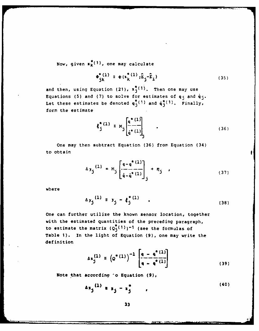
Now, given zK(1), one may calculate

* ( ) (*(1jk E E (35)

and then, using Equation (21), x (1. Then one may use

Equations (5) and (7) to solve for estimates of qj and qj.

Let these estimates be denoted q*(1) and 4(1). Finally,

form the estimate

Mi[77 1 1 ,(36)

One may then subtract Equation (36) from Equation (34)

to obtain

(1) i[q - * (1)S(37)

where

A Yjl _ Y_ zS (1)(38)

One can further utilize the known sensor location, together

with the estimated quantities of the preceding paragraph,

to estimate the matrix (Q!(l))- (see the formulas of

Table 1). In the light of Equation (9), one may write the

definition

3- (39)

Note that according 'o Equation (9),

Ax (1) a X * (40)

33

correct to first order. That is, correction terms on the*

righthand side of higher order in the difference xj - xj

may exist. Using Equation (39), Equation (37) now becomes

4 yj = Mj + (41)

Suppose one wishes to find, eventually, an estimate of

the state vector at an arbitrary time ti , an estimate that

is to be an improvement over an estimate that is simply

(1)

One then may expect it to be advantageous to introduce Ax i

as defined by

b . (i __ (.;) . 4, (1 ) -1i (43)

j ~ji ji /

This is a first-order version of Equation (26). The paren-

thesized quantities may be computed from Ri(1), derived from

Equation (42). The quantity axi is of course unknown, from

the viewpoint of the satellite observer. Its estimation will

be appropriate subsequently.

Using Equation (43), one finally may obtain from Equation

(41) the ob~eAvation equation

T* Ax.)b + ( (44)

Here

(45)

34

In the observation equation, note in summary that one

computes )j and Tji (from the observation vector Yj

and from the initial estimate 'k already assumed to be

available. The remaining quantities are unknown, although

subsequent analysis will assume knowledge of certain statis-

tical properties of j.

Further, note that for another observation at, say, time

tm, one will have redefined the quantity Ai such that it may

have second-order differences from the Axi of Equation (44).

The next subsection will ignore such differences in developing

an iterative procedure which-if convergent-will

eliminate their impact upon an ultimate estimate of zi.

D. Iterative Differential Correction

Define the following composite quantities for a set of

n observations:(1)

by 2 (46)

T* ()ii (47)* (I)

T

(48)

111

17 2

35

The composite form of Equation (44), j = 1, 2, ".- n, is

then

a Y(1) T ) Yi(1) + 17411 (49)

Note that this equation places no restrictions upon the

time separation of the sensor observations; upon the sensor

mix"; or even that necessarily t1 < t2 < . < n-1 < tn.

Suppose now that one can find an eW mato4 matrix W'1 (i.e.,

a function of 4( 1 ), which yields an estimate of 41i (M ) in

Equation (49):

L (50)

and which obeys the constraint (not an approximation)

wi T - 1 . (51)1 1

(The righthand side here is an identity matrix.) The next

subsection will provide a class of such estimators.

Whatever the specific version of wi(1), one can interpret

the result of Equation (50) as

laxim] * ii i (52)

using Equation (40). That is [dxil] is approximately an esti-mate by which the originally given orbit estimate %() (de-

rived from k(1) via Equation (42)1 was in error. One might

hope that an improved orbit estimate would be

* (2) * ( &s• (53)

36

One can now repeat the preceding process, replacing

Ii(1) by x (2) and obtaining[ &i(2)] * -* (2)a (2) (54)

Continued iteration leads to a sequence

1 *(2) 001il i 1'

which may converge, i.e.,r ]"'Lim IxL -) 55)k-w (55)

depending upon the form of W and upon the accuracy of theinitial estimate x4(1).

Suppose after, say, k iterations, one stops the iterativesequence, when there remains the estimated error

(k) [Ax i(k)] * (56)

Then the corresponding form of Equation (50) is

f (k) -Wj(k) LY

* W.(k)((k)A (k) )- W ( . +z 17)( 61 Ck) + w (57)

using Equations (49) and (51). The k-iteration analog ofEquation (40) is now

Ax k) a 58

37

a first-order approximation that may be quite good if sub-

stantial convergence has occurred. Substituting into

Equation (57) and rearranging,

(x. (k) (k)

This is a result of fundamental importance, since

it specifies the error in xi(k)-i.e., the orbit estimate

ultimately obtained from the entire process and that con-

tains within it, as a partition, the ephemeris estimate r*(k).

Assume now, and henceforth, that the convergence has been

such that f(k) is small enough to be ignored. Then for

simplicity one may denote x1 (k) as simply and W (k)

as just W* (i.e., showing its functional dependence upon xi),

to obtain

(I -X) Wi 0 • (60)

Later sections will analyze Equation (60).

E. Estimators

The purpose here is to define and discuss-but not

actually to derive-a class of estimator matrices from

which one may select a particular member for use in Equation

(50). The approach here is first to introduce two specific

members of this class, and then to generalize.

Consider a relation of the form

w= Tp + , (61)

38

in which:

o p is the true value of an m-vector whose estimate

one wishes to obtain

o w is a known "measurement" n-vector (n > m)

o is a random "error" n-vector, whose value is

unknown but some of whose statistical properties

are known

o T is a known matrix, not a function of p.

One wants to obtain the estimate p* via an estimator matrix W

in a relation of the form

I .= W., , (62)

under some designated optimization criterion.

Moreover, one desires the property that if is unbiased,

then the estimation error (p* - p) is also unbiased-i.e.,

one desires that W be an "unbiased estimator."

The unbiased estimator property translates into a simple

mathematical constraint. Substituting Equation (61) into

Equation (62),

S=WTp + Wt * (63)

Then if and only if

WT m , (64)

(the m x m identity matrix),

W? (65)

39

and if is unbiased then so is ( - p). Thus, the

£xactnee-k Cc tudian of Equation (64) is a necessary and

sufficient condition that W be an unbia~ed eztimato4.

To define a weighted Zeast squares criterion for esti-

mation of 41*, begin by defining the quantity

T , (66)

i.e., a noise-free measurement vector corresponding to gi.

Thus if p* is nearly equal to P, then '* becomes nearly an

ideal measurement. One might reasonably ask that W be chosen

such that the magnitude of u -. be minimal. One might also

ask that those measurement error components corresponding to

very accurate measurements be accorded the most statistical

weight. That fs, one might require that W minimize

n (W w 2

where (c )2 is the known variance of the ith measurement.

By carrying out an appropriate minimization procedure

while observing the exactness constraint (see Reference 2,

pp. 201-203), one can obtain the result

WLS z (W)eighted Least Squares

(TtC:lTf'I T' t-1 *(67)LS - CLS

Here by definition CLS is the n x n diagonal matrix with

nonvanishing elements

(CLS)" 2 * (68)

40

Several features of this result are significant. First,

it clearly satisfies the exactness constraint. Second, the

statistical properties of ? that must be known are its com-

ponent variances (i.e., knowledge of the form of its proba-

bility distribution is not necessary). Third, the form of

WLS makes the estimation result invariant with regard to

selection of %-component dimensional scale (e.g., km or NM).

(Note that if the weights 1/(o)? are arbitrarily set equal

to unity as in 'ordinary least squares" estimation, dimension-

scale invariance no longer holds.) Fourth, the inverse of

CLS is trivial to find, so that numerical evaluation of

WLS is straightforward even when the number of measurements

is large.

One may, however, adopt a different estimation criterion,

and arrive at a somewhat different result. Suppose one

decides to minimize, not the measurement residuals, but the

state-vector residuals-i.e., the individual component

variances of the estimation error (g* - 11). For rinimum-

vaiance estimation, one is to minimize each of the quantities

* 2(i " #) £il, 2,# --

again observing the exactness constraint.

If one carries out an appropriate minimization procedure

(see Reference 2, pp. 185-192) assuming now that the 'true"

covariance matrix D is )Pnown, one can obtain the result

WMV a (W)Minimum Variance (69)

- (T tDlT-1 TI T 1

41

Significant features of this estimator are as follows.

First, it clearly satisfies the exactness constraint.

Second, the statistical properties of that must be

known are its entire covariance matrix (not, as for WLS,

merely the diagonal elements of D). Third, WMV provides a

result that is properly invariant with respect to dimen-

sional scale changes. Fourth, the inverse of D may not be

trivial to find when the number of measurements is large, so

that numerical evaluation of WMV may not be straightforward.

Fifth, the Vadiance o6 each component o6 Ili - p) iz indeed

minimum 6o4 WV, az compared to the Ip* - pi)-omponent vat-

iance o6 any othet tWitmato4 (including WLS). However, how

can one obtain D with assurance?

In fact, D will not be exactly known in practice, but may

be approximated by some matrix C that must be real, symmetric,

invertible, and have positive diagonal elements. Then the

practical estimator will be

W M (T-tcIT) TtC-(

This reduces to WLS if C - CLS, and WMV if C a D, but in

fact represents a ttas6 oJ etimato4A where C is selectable.

Ease of calculation and estimation accuracy both depend upon

selection of an appropriate C.

One may show (see Reference 2, p. 202) that the esti-

mator of Equation (70) results from minimization of the

quadratic form

(T- .p) t - (7) :

subject to the exactness constraint. This generalized opti-

mization criterion is known, somewhat confusingly, as the

weighted tt&ut Aqasa491 4iteoe,.

42

6--

With regard to the preceding subsection, the following

correspondences hold for the kth iteration:

[ (72)

Y W 1(73)

174-- t (74)T(k) T

(75)w(k) ..Wi W - W

(76)

Note that since a value for 4(k) is assumed as an input

to each iteration, T1 (k) = T(,i (k)) is a known quantity as

assumed in the minimization of the quadratic error expression

of Equation (71).

The preceding discussion has not addressed three key

questions. Does convergence occur, in the iterative dif-

ferential correction process, for an arbitrary selection

of C? If, for a given C, convergence does occur, does itnecessarily yield a unique x1? (That is, does Equation

(60) have more than one solution?) If N! is unique for

a given C, what is the minimization criterion to which ii

corresponds?

In fact, convergence may or may not occur for a given

selection of C. Further discussion of this topic is beyond

the scope of this paper.

43

One may show, however, (see Reference 2, pp. 437-440),

that if convergence does occur, the limit ai is unique for*

that particular C. Moreover, the resulting xi minimizes

the quadratic error expression of Equation (71), wherein T*

is now to be interpreted as T(x).

Note, in closing, that all of the analysis of this sub-

section presupposes that the correct functional form of T

is known.

F. Calculational Strategies for Ephemeris Estimation

Suppose one must obtain ephemeris predictions for a se-

quence of times tk, k 1 1, 2, ...- that is, suppose one

must obtain a number of estimates xk from a given set ofmeasurements. Suppose, moreover, that during the time in-

terval of prediction, additional measurement data occasionally

become available. One then desires to obtain a revised set

of predictions xk in near-real-time with the arrival of

new data.

Calculational efficiency of ephemerides now becomes an

issue: is it necessary repeatedly to carry out the full

Iterative differential correction process for each ak?

Calculational strategies do exist to alleviate this prob-lem, at least under some circumstances. The first strategy

simplifies calculation of a set of sk from a given set of

measurement data. The procedure is first to find one state-

vector, say RI, via iterative differential correction, and

tnen repeatedly to utilize the relation

1k a #ki xj, kal,#2.. (77)

fsee Equation (42)).

44

One would hope to obtain in this manner-independent of

the choice of i-the same set %* as by direct use ofiterative differential correct ion for each x.A proof of

this equivalence will conclude this subsection. The strategyof Equation (77) is of quite general utility, involving no

restrictions as to the nature of C employed in W [see

Equation (70)].

Two further strategies, the "Bayesian filter" and the

"Kalman filter without driving noise," do involve such re-

strictions. The purpose of those strategies is to minimize

the recalculation of x!~ for Equation (76) when, from time

to time, new measurement data become available. The key to

their utility is treatment of each batch of new data as

having errors uncorrelated with errors of all previous data.

Thus, these strategies are useful for particular, block-diagonal forms of C. For such forms, these strategies provide

estimation results more expeditiously than, but identical with,

complete "brute force" re-estimation of x1 from old and new

raw data for a given C. Reference 2, Chapters 10 through 12,

contains a detailed discussion of the Bayesian filter and the

Kalman filter without driving noise. Their further discussion

is not appropriate here.

The promised equivalence proof will demonstrate that %kis identical, whether arrived at by iterative differential

correction or indirectly via Equation (77). That is, sup-

pose that iterative differential correction yields directly

at tk a value 1k' and directly at ti the value ii, whencea value xk obtains via Equation (76). The problem is to

prove that* (78)

k k

45

Now from Equation (60),

XI - 1W 7 (79)

and

Sk I *k = Wk " 17 '(80)

where the W-arguments are respectively %I and zk'. Given

Equation (77), then by Equation (26) to first order

k *k (* )xk-* - $(x i - x) , (81)

where

S ki + (82)

Premultiplying Equation (79) by ki and combining with

Equation (81),

2 k - 2k =ki Wi " 7 (83)

Now from Equation (70) and the correspondences of Equa-

tions (72) to (76), the general form of W i is

W. - (T*C * T l T*+ C-1 (84)

Using this, one may expand the lefthand side of Equation (84)

as follows:

46

- ~* j*t_-,_" )-

.Z TiW i " -Ti C T i " iki"-k"15

TC iki -1 k- *S)L-) T*tC

=[(T* 4.tc( i~) T . kC * (85)

The last step involves substitution of two subsidiary rela-

tions. The first is

_*_*I ki I= -ik , (87)

a restatement of Equation (29). The second is*

" ) 1 = (...*...)1. (87)-ki] = -

Now from EquatiLns (45) and (47),

* * (88)i ik 'Tk (8

Substituting this into Equation (85), one finally has

* *"-1 *")-1 T*tC-1"ki Wi = (TkC Tk k

(89)

= Wk

This relation holds for any invertible matrix A. Takingthe transpose of both sides of

A -'AA' l

one hasCA'l)t At -' 1(-" t At

Hence (A-1) is the inverse of A , as in

(A71)t a (At) i

47

using the definitional Equation (84). Upon substitution into

Equation (83),

k k'k - zk - Wk" - (90)

a relation identical in form with Equation (80). But as stated

earlier, such an equation has a unique solution, and Equation

(78) therefore must hold. This completes the proof as required.

48

III. EPHEMERIS ERROR PREDICTION

The preceding chapter describes linear-algebra method-

ology for estimating Keplerian satellite ephemerides from

sensor measurements. Specific estimation techniques within

this methodology depend upon selection of a matrix C, which

is some approximation to D, the covariance matrix of measure-

ment errors [see Equation (70) ff.).

The purpose here is to develop equations for estimating

errors in the ephemerides that would be arrived at by the

methodology of Chapter II.

Of the five ensuing sections, Section III.A defines the

error estimation problem in terms of inputs and outputs.

Section III.B derives equations of the general solution,

expressed in terms of the covariance matrices C and D.

Section III.D introduces specific representations for C and

D. Section III.E details the equations of the general

solution in terms of those representations. Finally, Section

III.F defines and discusses the ephemeris error equations

underlying the computer model SEEM.

The general solution of Section III.B here is well known

[see Equation (16), Reference 4]. A contribution of this

analysis is the representational discussion of Section III.C,

and specifically the analytical matrix-inverse given by

Equations (143) and (144). When used in the estimator W, it

affords calculational efficiency plus some accuracy improve-

ment over the conventional least-squares approach to emphem-

eris estimation.

The ensuing analysis assumes reader familiarity with

covariance matrix theory as reviewed in Appendix A.

49

A. The Error Estimation Problem

This section defines the ephemeris error analysis problem

in terms of assumed inputs and required outputs.

1. Assumed Inputs

Assume that the following inputs are available:

a. The epoch set tk, k - 1,2,..., for which ephemeris

errors are desired

b. A state vector xo corresponding to some epoch to

(affording a complete specification of the "true"

orbit of the satellite)

c. For each tj at which a measurement is made, the set

of quantities [see Sections II.A and II.C]:

qj, 4j, Mj , Aj, & € j , rTj

(affording a description of "true" observables,

the subset of these actually observed, and the sen-

sor position)

d. For each sensor the functional forms of Table 1

necessary to evaluate the matrix QjI from qj, 4j

(affording subsequent evaluation of Tji(x j ) [see

Equation (45))

e. Relative to the measurement error vector 17: its

'true" covariance matrix D; its covariance matrix

representation C used in the estimator W; the

assumption that 17 is unbiased, i.e., that 0.

50

The prior generation of input c. from appropriate sensor

characteristics is a standard space-surveillance problem not

within the scope of this report (although the equations of

Sections II.A and II.B are useful in solving that problem).

The assumption of e. that n is unbiased is subject to

the following interpretation. Suppose each observation

error-vector 77j [a partition of nj: see Equation (34)]

is what remains after application of calibration, atmospheric

refraction, and other known biaA corrections to the raw ob-

servation data. The error nj then comprises *noise" and"residual bias" contributions (see Section III.C). If the

probability distribution of each of these is symmetric about

zero, then 7ij = 0 for each tj and hence '" = 0.

2. Desired Outputs

Let Sk denote the covariance matrix of the error (%t - xk).

Let rSk be the upper lefthand 3 x 3 partition of Sk; i.e.,

let the elements

(rSk) -(, n, 1, 2, 3 . (91)

Then rSk is the covariance matrix of ephemeris error, since

r S E {U' - )

.* . ./

k/. r•)( k_ r k t(r k fk) Ui kE1 (92)

k 31 k ) kk k

Desired simulation outputs are

a. The matrices rSk, corresponding to the desired

epochs tk, k - 1,2,...

b. "Error ellipsoid" interpretation parameters (orien-tation angles, semi-major axes) for each rSk, where

orientation is specified relative to the U%' reference

frame [see section I.A].

Note (see Appendix A) that the interpretation of rSk in

terms of an error ellipsoid centered at rk is legitimate

only when the probability distribution associated with

(rk - rk) is normal and unbiased. This condition is met whenever

the probability distribution associated with 17 is normal and

unbiased, since by Equation (61) the error (x4 - 'k )

[containing (r - rk ) as a partition] is a linear

transformation upon i1.

B. General Solution

The purpose here is to derive general equations giving

desired simulation outputs as a function of assumed simula-

tion inputs.

Consider Equation (60), written for an arbitrary epoch ti:

S " -i Wa. 17 (93)

Subsection II.F has established the formal invariance of this

first-order approximation [see Equation (58)] under the epoch

transformation Equation (26)t itself induced by Equation (21).

The theorem represented by Equation (A-18) allows one im-

mediately to write

Sims Wi D Wi ,(94)

52

The lefthand side is a desired simulation output, but the

righthand side depends on the quantity zi-according to

Section III.A, not an available input.

But via the Taylor expansion in vector form,

* aW. E W(zI )

a W(xI2 + Cs .)*(5

1 3I.

One can see that the order of approximation of Equation (93)

is preserved in writing

a

xi - Xi - W. • (96)

The W i here is a function of xi , not xi:

W -W(xi)

- TCT 1 1T (97)

(see Section II.E), with Ti a column matrix whose general

partition is

[!see Equations (45) and (82)), where

Z jim = ¢Jl j(i96b)

Evaluation of Equations (98) is for

" # jo a • (99)

53

Thus

S. * W. D W. (100)

and since

Rk Xk t ki ( " i (101)

one has

Sk SkiS - (102)

Equations (100) and (102), together with Equations (91), (97),

and (98), give tie desired outputs a. as a function of the

assumed inputs a., b., c., d., and e.

It remains in this subsection to obtain the output b.

from rSk expressed thus far relative to the inertial (xyz) frame.

By Equations (13) and (A-18),

rs] - L r Sk • (103)

Diagonalization of lrSk]uVW, if carried out by an appropriate

numerical procedure, yields eigenvalues (01)2, (02)2, (c3) 2

and corresponding normalized eigenvectors, which one may denote

&S el, e2, t3. According to the analysis of Appendix A,

the semi-major axes of the 01-a" ellipsoid have values 01,

a2, o3.

54

One way to interpret the ellipsoid orientation is as

follows. Pick the first eigenvector el, and denote the

angles between el, and U, V, W as 011, 012 , and 013, respec-

tively. Then

cose 11 = U , U (104a)11,1

cos 012 = ,104b)

cos 13 e (104c)

where

U i , 1 %N 0 (105)

These are the direction cosines of the orientation of thea,-axis of the error ellipsoid. Note that one may

arbitrarily change the sign of el if ease of interpreta-tion of the angles is improved thereby. Such a change does

not upset the normalization of el and physically meansthat one may take either of the "al-ends" of the

ellipsoid to be "positive."

One can interpret each of the remaining eigenvectors

similarly, .completing extraction of desired outputs b.

C. Measurement Covariance Matrix Structures

The purpose here is to introduce some candidate algebraic

structures for the "true" covariance matrix D. These, perhaps

with still further approximations, are also candidate struc-

tures for C.

55

The first of the following subsections introduces struc-

tures by consideration of the "noise" and "residual bias"

concepts menticned earlier. The second subsection further

details this structure into a form which, although of

limited generality, does permit analytical extraction of

the matrix inverse-of importance since one would like

to use W with C = D.

1. Basic Structure^ Im

Let each observation epoch ti now be denoted as t.,

where a indexes the sensor making the measurement; m indexes

satellite "pass" through the field of view of that sensor;

and j is now to be regarded as indexing an observation

within a pass.

Consider the structure of D first with regard to parti-

tions corresponrling to each observation epoch a and then

with regard to the "microstructure" within such partitions.

a. The General Observation Partition

Let the observation error vector a correspond tothe epoch t Let the ordering of the anm within thet h ew i h i e p ch 0 te

composite vector ' (see Equation (48)] be hierarchic, such

that a varies the slowest, m the next slowest, and j the

fastest. The ordering of other composite vectors and of the

matrix D will of course correspond. Note that freedom to

select this indexing hierarchy exists, since up to this

point the analysis has not restricted interpretation of

the sequence tj (see II.D).

Now introduce the decomposition

IV " u + (106)

56

In

wi' ,the requirement that the term ej account for any cor-

relations that may exist from one observation to another.

That is, Vj is to be interpreted as a "noise" term and (jOM

is to be the "residual bias" term within qj. It follows that

k = jk ' (107:

where

Mathematically, this decomposition entails to this

point no loss of generality. Physically, the desirable

interpretation is that the a result from random receiver

and possible random external noise sources, with each"observation" actually deriving from some small data set

such that, for appropriate observation spacing, Equation

(107) holds. This physical interpretation clearly implies

some practical constraints as to signal processing, anda m

moreover implies that always Gj is positive definite.

Regarded as residual bias errors, the tj by contrast

will be correlated with each other from one observation to

another, at least for observations not too widely separated

in time and made by the same sensor. Thus, one might set

E 1 nt C, j, nl (109

8 6 umn (1106cj &jk

assuming no correlations from one sensor to another.

57

Then by the symmetry of Equation (110),

aI CL. aHnm

jk (111)

, H7 will be non-negative definite, taking into ac-Ascount that residual bias errors may sometimes vanish.

Finally, assume that the noise errors are uncor-

related with the residual bias errors:

= o 0

(112)

Taking all of these relations into account, the

general observational partition of D is then

S 0(113)

a ('G 6 6jk 'H ) (114)C=B mnjk + ajk)

with

jk kj (115)

The resulting D is-as required-real, symmetric, and

invcrtible, and has positive terms on the diagonal.

Note that sufficient conditions for 1 to be unbiased

are

S- 0 (116)

58

and

CL0 (117'

Physically, one can regard these as averages for each sensor

over large ensembles of observations, with probability dis-

tributions symmetric about zero.

b. Microstructure

Now consider the problem of representing structurem ot fll

within the matrices Gj and Hjk. As will soon appear,

there is a problem in establishing a reasonable notation in

which that structure may be specified. This problem will

receive primary attention here. Possible functional depend-

encies of certain quantities will receive limited considera-

tion.

a^ M a MIn the present notation, observables at tj are

and qj, representing a range and two angle variables, and the

rates thereof. Some subset (possibly all) of these six quan-

tities is actually measured, resulting in the errors of Equa-

tion (106). If one indexes the components of that Equation

by p, p < 1,2,..., <6, then*

(%j)p - ( /0 / (118

One may now introduce a useful representation for

"O as follows.

* The index p relates to the components of qj and q- notdirectly, but via the sensor characterization matrij tMM

previously denoted Mj [see Equation (33)].

59

Define a matrix of standard noise deviations Vlj

as having the general element

j P C g(W /) p (1119)

where

(V %, J/pkvj)P I (12f

(Here q a 1,2,..., an index having nothing to do with the

vector q.)

Define a matrix of noise correlation coefficientsamvRj as having the general element

VJ .'pq 1, p = q (121a

otherwise

(v/ipq = ( )p\ V q (121b

Then from Equation (108),

"G -z z 0R- zj * " (122)

This representation Of Gj separates the standard deviations

of the components of A' from the correlations among them.

One may expect that the correlation matrix will depend upon

the control-system design of the specific sensor 0. If the

60

CL m OLcomponents of vj are uncorrelated, Rj reduces to the iden-

tity matrix. One may further expect that the size of the

standard deviations of error components will depend in general

upon si nal strength and receiver noise. That is, one expects

that v j will be a sensor-dependent function of qj, qj,

and perhaps also of some parameter set 22 associated with the

target-e.g., radar cross-section.mnn

A representation for Hjk, analogous to Equation

(122), is obtained as follows.

Define a matrix of residual-bias standard deviationsa m

m as having the general element

(cx~y . 6%m'~(123)

where

Define a matrix of residual-bias correlation coef-a mn

ficients cRjk as having the general element

( R a 1 if p - q and m n and j k;cjh)Pq

=0 if (c~ r=0k € J por can ];

otherwise

61%) (icn)CI (125)

61

Then from Equation (111),

aHI= I . a (126)jk r j E jk E k

As before, this representation separates the standard devia-

tions of the components of and from correlations

among them. If the standard deviations of residual bias do

not change with time,

£ej c k (127)

However, this may not be the case, as when atmospheric re-

fraction corrections are imperfect at low elevation angles.a M am

Then t zj is a function of qj, and Equation (127) is

only an approximation.Q mn

The form of the correlation matrix cRjk will depend

upon the sensor. Its elements will tend to diminish for

large time separations I tj - tkI. For small time sep-

arations one may expect that

E jk C in (128)

a mIf the components of j re uncorrelated among themselves,

L IM a MMthen CRjk will be diagonal and £Rjj will be the identity

matrix.

2. Further Structure

The purpose here is to introduce further assumptions about

the structure of D that promote ease of inversion. All, some,

or none of these further assumptions may be valid for a givenproblem.

62

a. Occasionally Decoupled Passes

Suppose for sensor a there exists some time intervala zero, which is the minimum separation between observations

over which residual-bias error correlations vanish:

a R nk= 0, la - &^ntl Qe jk k z

Then by Equations (114) and (126), a condition on the general

observation partition of D is

-jk o, 1 0

(130)

Of interest here is the case where the separation be-

tween passes by sensor a occasionally exceeds aT zero. (That

is, the assumption is not made that every a-pass separation

is larger than C'zero-)

To arrive at an appropriate mathematical formulation

of such a situation, define an index L = 1,2,..., which

counts pass separations for which

Q~m+j a m Q aI - zero (131)

here atm + 1 is the first observational epoch of pass m+1 for

sensor a, and atm is defined to be the last observational

epoch of pass m.

Such pass separations decompose the a-pass sequence

into a sequence of *multiplets," each comprising one or more

passes. Hence one may consider L to be the index of de-

coupled pass multiplets.

63

Now L is an index dependent upon a and m:

L - L(, M) • (132a

One may express the functional dependence upon m recursively.

Let

L(a, 1) B 1 * (132b

For arbitrary m, if Equation (131) holds

L(a, m + 1) - L(m, m) + 1 ( 1133a

otherwise

L(a, m + 1) - L(a, m) (133b

Now let

L E a C U (134a

under the constraint that passes m and n are in the same

multiplet:

L(a, in) - L(, n) * (134b

The assumption of occasionally decoupled passes is just

a. mn CLL h.Hjk L(a, m), L(a, n) 1135

[see Equations (126) and (129)].

Utilizing the redundancy

un 6 L(a, m). L(c, n) an (136)

64

one may now write Equation (114), subsuming Equation (130), as

jk Q0 L(ci, mn), L(ai, 6 6 mn *k - (137)

Thus D is block diagonal. If the blocks of D are denoted OLD,

then the problem of inverting D reduces to that of inverting

the set of smaller matrices aLb.

b. Strongly Coupled Passes

Suppose for each sensor a there exists some maximumtime interval 'T one' for which residual-bias error standard

deviations and correlations are invariant-i.e., Equations(127) and (128) hold when

~tj - ti n (138) 'In particular, suppose one is greater than the

duration of any pass multiplet as defined in the previous

subsection. Then Equation (138) holds whenever

L(a, m) - L(a, n) (139)

and over each multiplet one has an invariant matrix

aLlMmn (140)jk (140)

One may refer to this as the assumption of At&on gy coupted

A necessary, but not necessarily sufficient, conditionfor the existence of multiplets that are each strongly coupled

internally, yet are decoupled from one multiplet to another,

is that

ITone <C zo ° (141)

65

For example, if a zero happens to be one satellite period,

then each multiplet can comprise but one pass. For a low-

altitude satellite, if aT zero - 12 hours, then each multi-

plet might consist of a pair of passes on successive revolu-

tions. For some problems, Equation (141) cannot be satisfied

for multiplets.

When, however, Equation (140) is valid, substitution

into Equation (137) yields

oDn =8 8 6G68 + IH) (142)jk as L (a m)L(a, n)\3mn jk

When D has this structure, the general observational partition

of its inverse turns out to be available analytically:

a$(D-1)nn -6 6

-T_ 7 aLU OtLH(G)1'] , (143)

= 6.jk3

where

aL(a, m) U + aL 6, (, m) L(a, )(G ) (144)

These expressions for 3kconstitute a general-ization of the results of Appendix C. That appendix derives

the inverse of a matrix having its general partition of the

same form as

aG M 6 jk + H

66

[see Equation (142)], but with the restriction that Gy and

must be diagonal. That restriction allows those two

matrices to commute.

However, the result of Equations (143) and (144) em-bodies no such restriction, as one may show by proving that

those Equations yield the proper result for an inverse:

My~m . CO L 6~ 6 6) (145)j* .. aL mn-jk

The proof proceeds by direct substitution of Equa-

tions (136), (142), and (143) into the lefthand side here:6am y . £G 16

6 yG m 6ji 6yo(Gj\- Ln 6ikyti

S y 3 6 m £ i " Ly x(y,) , L (, n) i6

kL H 6ik

y L (,6L(, m) ,L(y,, L) LHn 6ye 6L(y, 1), L (8, n)G )Uk k)yti

aLG - aLL .~i( n O= 6al 6n 6j

m6c 6L (, m) L(0, n)

c L G 6n•G

00( 6L(a, M) L (a, n ~)(,mmj

S(146)

67

The last term here is a sum over just the multiplet L, and

has no nonvanishing terms over that multiplet. Since H and

0%u are constants over the multiplet, one can factor them from

under the summation. Moreover, one can see (via a 'truth

table" analysis) that

6 L(a, m), L(a,1) 6L(a, .), L(0, n) 6L(a, m) L(a, n) 6L(, i) L(a,L) (147)

Hence one may continue to develop Equation (146) as-6as 6 6j

+ 6 6 aL U aL H +aL Hcgs 6 L(, m) L(a, n) )

IH ~\ i ( , G H]~ • Oj~

=6 0 6n 6jk

+6a 6L(, in)L(, n)[eLH +

.6L(a, m) L(aL) (148)

Us 6a 6jk

as required. The last step above resulted from substitution

of Equation (144) for ULU.

With regard to Equation (143), note that D- 1 reduces

to a form block diagonal in (Gj) - 1 if all the UI happen to

vanish. Thus, one may regard D "1 as the difference between

a *noise" covariance matrix and a *residual bias* correction

matrix, respectively the first and second terms of Equation (143).

68

D. Some Expansions of the General Solution

The calculational efficiency of state-vector estimation

depends upon the degree of difficulty of extracting C-1 in

the estimator W i [see Equation (70)]. In "least squares"

estimation, C is taken to be diagonal--or at least block

diagonal, where each block dimension is of the order of the

observation-vector dimension. Such a C may be very different

from D, if the latter contains extensive correlation terms

among residual-bias errors. Then resulting ephemeris errors

will be worse than the optimum (minimum-variance) errors when

C - D.

Of course, one may choose C to be a better approximation

to a highly correlated D, but generally at significant cost in

calculational practicality.

The purpose here is to find explicit, detailed represen-

tations for Si, the covariance matrix of state-vector

errors, for various combinations of some possible structures

for C and D. Each Si representation will exhibit a char-

acteristic level of approximation to the minimum-variance

form (when C = D) and will also afford a characteristic

level of calculational efficiency not only for W i , but

also for Si .

Structures of D considered here derive from the previous

section. Structures for C considered here also derive from

the previous section, but will occur in a distinctive nota-

tion in order to avoid confusion with D.

69

In the interest of notational simplicity, the ensuing

expansions of Equation (100) will omit the subscript i. The

quantities S, W, and T are still to be understood as corre-

sponding to the estimation epoch ti. The indexing conven-

tion of the expansions will be the same as in Section III.C,

i.e., it will correspond to the observational epochs t).

Results will occur as formulas for X- 1 and Z, where

X T (TC'1T)"1 (149)

and

Z (C 1T)t I(C-1 T) (150)

Then, taking into account the symmetry of C,

S - XZX (151)

Also,

W x(ClT) (152)

Note that if C - D, then S a X. Thus X is the covariancematrix of state-vector errors for the case of optimal,

minimum-variance estimation. Accordingly, ZX (or XZ) is the

matrix factor on X by which S falls short of optimality.

Nimeric inversion of X- 1 to yield X is not ordinarily a

significant calculational problem, since X is only a 6 x 6

matrix and need be inverted only occasionally [see discussion

of Section II.E and Equation (102)). Bence, one may regard the

calculational difficulty of finding W and S as effectively asthat of finding X- 1 and Z-the latter of course con-

taining C-1 T [see Equations (150) and (152)].

70

Table 5 gives seven combinations of structure assumptions

for C and D, along with appropriate analytic expressions for

C-1 . Table 6 gives corresponding formulas for X-1 and Z.

The notes in Table 5 pertain, first, to calculational

ease of finding X- 1 and Z, given a set of measurement data;

and second, to ease of recalculating X-1 and Z as new

measurement data become available. Additional comments upon

each case will conclude this section.

Case I imposes no restrictions upon C or D, except that

all error correlations vanish from one sensor to another.

These matrices are then block diagonal, respectively, in

partitions OC and OD. The formulas for X- 1 and Z are alge-

braically simple but calculationally complex, requiring nu-

meric inversion of the large partitions OC.

Case 2 introduces the structure of Equation (114) for D,Smand a similar structure for C in terms of Ej (analogous

to 0 j) and (analogous to IHj). These structures

improve the physical interpretability of C and D, but are

generally still not calculationally practical in that inversion

of each of the large partitions OC is still necessary.

Case 3 reduces C to a form block diagonal in 0E, resulting

in a least-squares form of W. However, careful inspection of

the expression for Z in Case 3 will reveal that the generality

of the D-structure places significant demands upon computer

memory in recalculating Z as new data become available.

71

A 414 aa.* ~~ at * U

h.S 0 Lb 61a 4 er-~~6

b.0 4 h

61 _1 4 .1 .4 0~4b. , S -.0 £ a. c q4 1 a0 is .

L OC 4a 4 -1

do w 9-. a41CO i I 2m 0 C C

1 or onj Av 0U u 4 l A 0 aO " -r

11 h e; 24 0

w 0 4 .t 04 a v0

*- A'~ 4 u8 a

0 0 6 Aaa2.6

r. oc .6 0 ir U: 60 X IaM~0 0 C,'A

Obm 0 Is - 401 rC4151 rn-siofu-a0 1 1. o

. C. c0 s a. 4- a v-

x 0 0 0 0 0 0 0 00 0 0 0 0 0 0 00 0 0 0 0 0 0 0

z--

9 $4

u -

.1L

Ja

a 3

72 .

a Ac.31

LO a

(co IL ~ M .

udCC- a a -D. &..- a. -0

CC I. &bJU- M -

u cc --

N~~~~... ......-... ga - a

PIC~ ~. i-- - - '3

a.-*-1h ~ ~ 4- 4

.-- a a- a3

Case 4 begins a different type of structuring, relative

to Case I as a baseline. A pass-multiplet structure for C

and D substitutes the problem of inverting the partitions aLC

rather than the aC. The aLC tend, however, to still be of

large dimension.

Case 5 is the pass-multiplet analog of Case 2 and is

calculationally not greatly advantageous to Case 2.

Case 6 introduces a structure for C analogous to Equa-

tion (142) for D. The inverse of this structure exists in

simple analytic form and makes calculation of C-1 only

slightly more involved than for the least-squares Case 3.

Thus, the inversion Equations (143) and (144) effectively

afford a limited, calculationally efficient generalization

of least squares estimation.

With Case 6 as with Case 3, however, the general form of

D does impose some calculational penalties in regard to Z as

new data become available.

In Case 7, both C and D have the structure of Equation

(142). Calculation of Z is thereby considerably simpler.

(Further specializations of Case 7 will appear in the

next section.)

E. The Computer Model SEEM

The purpose of this section is to describe the analyti-

cal basis of the computer model SEEM (see Chapter I). A

further purpose is to provide some numerical outputs

of SEEM as examples of calculational results obtainable

using the analytical formalism of this report.

74

I. Analytical Basis of SEEM

The approach here is the further specialization of Case 7

of the previous section.

For D, assume that each pass multiplet is a single pass.

Further, assume that aLH is the same for every multiplet.

Then one may write

csDmn = 6 6. (6k C G + H) (153)

Make further assumptions about the internal structures

of aGl and LH. Assume that within any given observation

the noise errors are uncorrelated with each other and the

residual bias errors are uncorrelated with each other. Then

both aO (see Equation (121b)] and aR [see Equation

(125)] are identity matrices.

Then from Equations (119) and (122), the general element

of aGP is

(3G/)pq Pq(; (154)

From Equations (123) and (126), the general element ofOH is

-pq 6pq(kC) p (155)

75

SEEM at present provides for just one sensor type, radars

operating in altazimuth coordinates (see Section II.A).* The

noise-variance components of Equation (154) become

av a CL 0°/ (I/Cos h )2(5M) X2 t(156)

2 2(a~) a ( 01h) (157)

a ~2 (~2

Here X, h, and P respectively denote azimuth, elevation, and

range, and the symbol a on the righthand side represents a

constant for a given radar. The factor (1/cos h)2 in

Equation (156) accounts for the loss in azimuthal accuracy

at high elevation angles.

SEEM assumes the following for the residual-bias variances

of Equation (155): 22a 0)2 (C~

C (159)

(160)

(161)

* One may also, by an input strategem, make SEEM accommodatealtazimuth-coordinate telescopes. The strategem is toassign a very large value to 0c 2 of Equation (158),thereby assigning range measurements negligible statisticalweight.

76

Again the o symbols on the righthand side are constants

for a given radar.

As regards C, SEEM provides two options. The first,

a "least squares" option, is

cs) 6mn 6 a G m(162)B CLS jk 640 6mn k G 112

The second, a 'minimum variance" option, isas mn iS.m

jk - Djk (163)

Appropriate manipulation of Case 7 results of the pre-

ceding section then yields for the least squares option I

SLS M - + L ( NP) ~XSX L~ M (164)

where

and

For the minimum-variance option,

SMVinXNV * (167)

77

where

a (16)

and

~Lm \ / (169)

Evaluation of the Tr in these expressions is via Equa- itions (98), since Tj there was redesignated at T3 in the

notational change of Subsection III.C.1. On the righthand

side of Equation (98a), the MJ is the "radar" entry of

Table 4. The QI-I are those of Table 1, as specialized in

Table 2. Appendix B gives expressions for *ji and +ji of

Equation (98b).

Thus, SEEM evaluates SLS or SMV as Si at an appropriate

time ti . Equation (102) then yields Sk at requisite pre-A A

diction times tk, k - 1, 2, ... n. For each tk , SEEM ex-

tracts rSk from Si [see defining Equation (91)] and then

obtains [rSk]UVW via Equation (103), evaluating the rotation

matrix L as developed in Section II.A.

The diagonal elements of IrSk]UvW are the variances02 U02 P02kV k kW, respectively the radial, along-track, and

cross-track component variances of the ephemeris vector at

tk. The resultant-vector variance is

a 2 -2 * a 2 + a 2 (170)k Uk *Vk Wk

78

SEEM outputs 3ak, 3akU, 3:kV, and 3ckW for the predic-

tion times tk, k = 1, 2, ... , n.

As it is now programmed, SEEM does not obtain the prin-

cipal axes and orientation of the ephemeris error ellipsoid

by diagonalizing [rs k ]UVW, etc. However, for near-

circular orbits this ellipsoid tends to be oriented along

the UVW coordinates, primarily because of the effect of

period uncertainty, which makes the along-track error ordi-

narily large compared to radial and cross-track errors.

Thus, for near-circular orbits one may regard 3 OkU,

3-kV, and 30kw as approximately the principal dimensions

of the 60.8-percent confidence error ellipsoid (see Table A-i).

The resultant 3ok is the exact RSS dimension of the ellip-

soid, since the trace of IrSk] UVW is invariant under the

coordinate-frame rotation of diagonalization.

2. Representative Ephemeris Error Results of SEEM

This subsection gives representative graphical outputs

of SEEM. All outputs given here correspond to a satellite

in circular orbit at an altitude of 400 km. The epoch t - 0

is that of 'launch," when the satellite initially appears in

orbit.

Sensors are altazimuth radars, with hemispheric coverage

down to a minimum elevation angle of 7. Maximum range is

set, not by radar capability, but rather by horizon line-of-

sight cutoff at minimum elevation. Sensors provide measure-

ments it 6-second intervals while the satellite is within

79

coverage. For "nominal" measurements, "noise" and "residualbias" standard deviations are those of Table 7.

SEEM output graphics of Figures 3 through 6 correspond

to the specific input conditions of Table 8. Figure 3

represents a pass through radar coverage about 15 minutesafter "launch." Error plots commence a few minutes after

the satellite exits coverage, simulating a data-processing

delay in availability of estimated ephemerides.*

Note that for this case, minimum-variance estimation

yields little accuracy improvement over least squares

estimation.

The error curves of Figure 3 exhibit several typical

features that deserve comment. First, the cumulative

growth of along-track error is what one would expect from

error in estimating the satellite period. By contrast,

the radial and cross-track errors repeat with each satel-

lite revolution. Thus, along-track error soon dominates

the resultant error.

Second, all error components contain the satellite period

(100 minutes) as a fundamental harmonic, with minima at or

near one-period intervals from the radar pass. This be-

havior is not surprising, since the radar pass corresponds

to a point in inertial space where position is actually

measured, i.e., where both estimated and true orbits are

closest together.

*In Figure 3, the width of the *radar coverage rectangle"denotes time in coverage, but the height of the rectan-gle has no interpretational significance.

so

TABLE 7"NOMINAL" STANDARD DEVIATIONS OF MEASUREMENT

,Coordinate Noise Residual Bias

Azimuth - 0.050 a - 0.05"

a CElevation c h a 0.05£ a . 0.05*

Range aO - 5D m. X0 a 50 M.V p P

TABLE 8INPUTS FOR SEEM EXAMPLES

Std. Deviations of Measurement Pass EstimationFigurePss staio

A umber Noise Residual Bias Spacing Method

3 Nominal Nominal -- sqeast(Solid Curve Squares

3 Nominal Nominal Minimu(Broken Curve Variance

4 Nominal Zero - S and M'Same Curve

5 Nominal* Nominal* 1/4 LeastRevolution Squares

Noinal* Nominal* 1/2 Least

Revolution Squares

* A&pIles to both redars

81

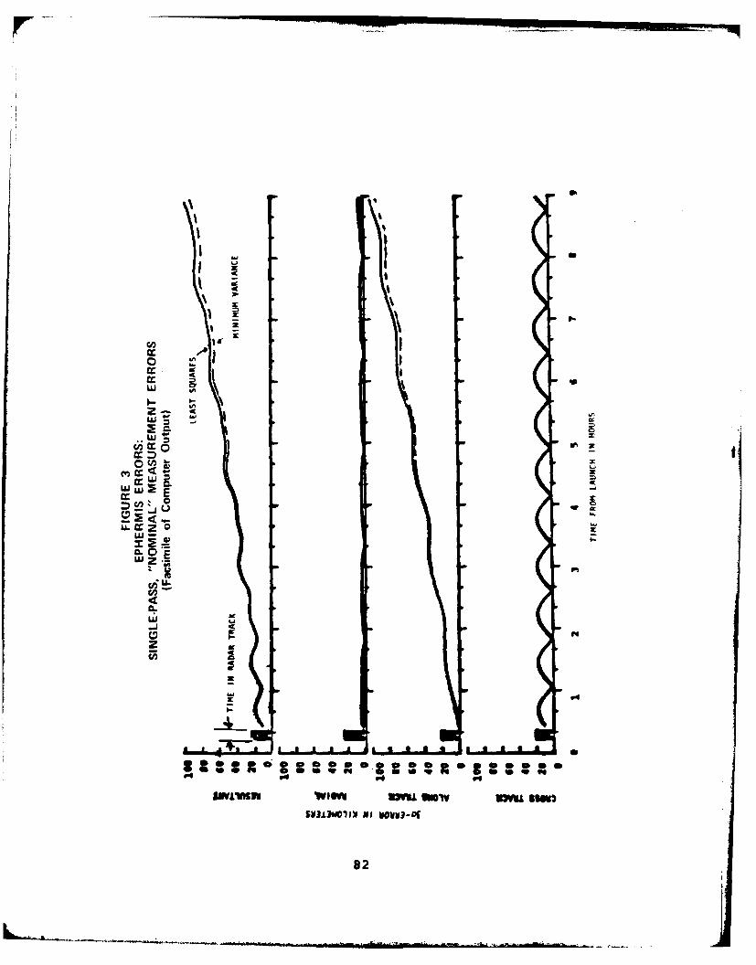
I z'

w SP

w

00< I-

wccz 0

w EzI

Li(DC

za

46 A,-

A-q

SV3L8 unI Now mm 9M3-3

82

0

zaz

LJ EwN) o

cr uj X

LUN0

Ca

z

83

CDC

2t

w M

w~

04.

MWL~sr Tfl %2u No %U in

SU3.LJbD1fN NI UVUI-Dg

84

cr 0-

U.~cc --

CLC

0K

NMI NW XM SSW%V313olluI vow].x

imb.

Third, the cross-track and radial errors clearly possess

a second harmonic in addition to the fundamental. One can

understand the structure of the cross-track error by re-

membering that the estimated and true orbital planes inter-

sect on a line running from the (minimum error) measurement

point through the center of the Earth and beyond. One thus

expects-and obtains-a second cross-track error mini-

mum where the orbits (nearly) intersect 180* away from the

pass point.

The more complex structure of the radial error probably

has to do with the interplay of two estimated orbit

parameters: the argument of perigee and the orbit eccen-

tricity.

Now compare Figure 4 to Figure 3. "Perfect calibration"

of the radar (i.e., zero residual biases) yields a dramatic

improvement in all ephemeris error components. One can

demonstrate, in fact, that most of the improvement results

from elimination of the residual bias in elevation.

Figures 5 and 6 both contain a second radar pass, with

measurement errors the same as for Figure 3. The additional

data in both cases lead to more accurate ephemerides, as one

would expect.

Comparing Figures 5 and 6, it is not surprising to findIthat the larger pass spacing yields a more accurate satellite

period, and hence reduced along-track figure error. The ra-

dial error is also slightly better for diametrically opposed

points on the orbit.

86

On the other hand, the quarter-orbit spacing of the passes

should stabilize the estimated orbital plane (which must con-

tain the center of the Earth) better than half-orbit spacing.

Thus, one may understand the reduced cross-track error of

Figure 5 relative to that of Figure 6.

In all of the foregoing examples, the pass geometry is

such that the satellite flies almost directly over the radar.

Reference 5 contains SEEM output examples for other pass

geometries, for lower minimum-elevation angles, and for as

many as three passes.

87

REFERENCES

1. Wright, L. C., SateZZite Ephemeris Error ModeZ:VaZidation, (in press), Analytic Services Inc.,Arlington, VA, 1980.

2. Morrison, N. introduction to sequential smoothingand prediction, McGraw-Hill, New York, 1969.

3. Herrick, S., Ast-odynamics, VoZ. 1, Van NostrandReinhold, London, 1971.

4. Prislin, R. H., TRACE 66 Orbit Determination Program,VoZume V: DifferentiaZ Correction Procedure and Tech-niques, TOR-006(93200-2, Vol. V), Aerospace Corp.,Los Angeles, CA, April 1970.

5. Kirkham, J. N. and L. C. Wright, Effects of SensorLocation and Accuracy on Ephemeris Prediction, (inpress), Analytic Services Inc., Arlington, VA,February 1980.

I-iELIDG F" BLANK-WIT 771AM

89 -

AD-AlGA 477 ANALYTIC SERVICES INC ARLINGTON VA F/G 22/3THE PREDICTION OF SATELLITE EPHEMERIS ERRORS AS THET RESULT FRO--ETC(U)AUG Al 8 E SIMMONS F49(,20-77C-0G2

UNCLASSIFIED ANSERSPON-80- NL

EN D

- OT 1

11111.211 _5 111IIIII-1.25 ~ IIBI IIBLU..

II

APPENDIX A

COVARIANCE MATRICES: DEFINITION AND PROPERTIES

THE PREDICTION

OF

SATELLITE EPHEMERIS ERRORS

AS THEY RESULT FROM

SURVEILLANCE-SYSTEM MEASUREMENT ERRORS

mmmnoimm num

APPENDIX A

COVARIANCE MATRICES: DEFINITION AND PROPERTIES

This Appendix provides a review of the definition and

primary properties of covariance matrices. The first sub-

-section gives properties not restricted to any particular

probability density function. The second subsection treats

covariance matrices for the special case of normal (Gaussian)

distributions.

1. Definition and General Properties

Consider an arbitrary random n-vector

w-p+ , (A-i)

where p is the true value of * and n is some random error,

such as measurement error.

Let the probability density function of j7 be p(q). The

probability density of the ith component is then

Pi (r ) = '" pwq R (tn ) (A-2)-m -- k#i

(The subscript on Pi indicates that its functional form may

depend upon the value of i.) The joint probability density

of ni and nj (where iij) is

PjCj hiri IJ p (7) 1 (dik) (A-3)

k#j

A-3

AM ....- T 1

Clearly this function is symmetric:

Pij()i.lj) " Pjilj,i i ) (A-4)

With these definitions, the probability that ni lies in

the interval [a,b] is then

b

I Pi(n)dn .a

The probability that T)i lies in [a,b], while also rj. lies

in [c,d] is

d b

I f Pi (ni j) didn •C a 0

Now define the expectation vatue of any function

f(17) as

E{fk() f f (17)P(1) n drk) . (A-5)-k=1 k

Then

-~i f f liP('lidi.

Ei ) d(A-6) -

the mean of , i. If Wn 0, then Is said to be unbia&ed.

A-4

I

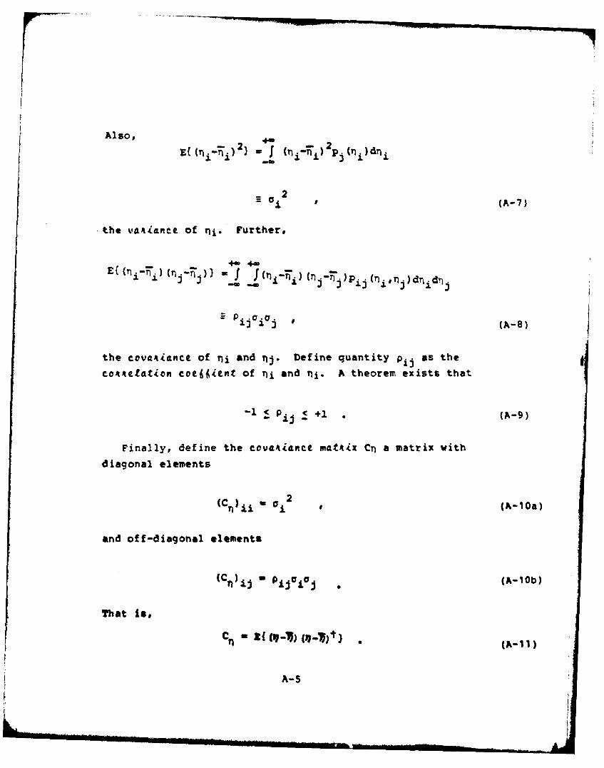
Al so,

E 1 i% Tj ,i Tj p.(n.)drj.

(A- 7)

the voa~ine of ni. Further,

Ef rii Fa 5Tj F J( 1 ~ ( . . P. *(f., in drj.dn,

l~lj U

the CoVd o&MCC of ni and nj. Define quantity pjas theCo44ettOM COe6~iEnt Of rnj and ni1 . A theorem~ exists that

-lp<.. ij1+1 . (A-9)

Finally, define the C0V&AidRCC wdt~J.X Cn a matrix withdiagonal elements

(C2 *(Ak- IOa)

and off-diagonal elements

(C1 * Pij OOL a (A-10b)

That is,

A-S

Note that one may estimate C .1 from a set of data sam-

ples (1)k, k = 1, 2, ..., K by replacing the integrals of

Equations (A-6) and (A-7) by sums over the index k, providing

that the joint probability functions pij(ni,nj| are known

(or assumed). (This report does not pursue further the sub-

ject of sampling and subsequent estimation of C .)

Clearly C n is symmetric. If all the ni are linearly

independent, then

-1 C P i < +1 (A-12)

and one can show that Cn is positive definite-i.e., its

inverse Cin-. exists.

Now consider the transformation

- F17 (A-13)

where is an m-vector (m<n) and F is any m , n matrix that is

not a function of q.

A functional dependence of t on 01, such as that in

Equation (A-13), means that for every point occurring in n-

space a corresponding point exists in t-space. Thus, for

any arbitrary volume V in 17-space, the same number of

points must occur in the corresponding volume V in

t-space:

V 11

A-6

Here the subscripts on the probability densities denote that

their functional forms are in general different. But since

V is arbitrary in Equation (A-14), it follows that

P (t)d; d;l''d n P1(7)d)1 ... d n n (A-15)

This is a fundamental invariance relation for functional

transformations among random-vector spaces.

It now follows that

+- 4-a

1C m

-+= m= f-.f F77p (17)dnl..dj

- F*E{17) , (A-16)

that is,

P17 . (A-17)

Similarly,

c- F.C • (A-18)

Note that neither Equation (A-17) nor (A-16) is necessarily

valid if F a F(o).

According to Equation (A-17), if 1 is unbiased then Cwill also be unbiased. Equation (A-18) tells how to calcu-

late the covariance matrix in ?-space. One can show that

A-7

the symmetry property of C Is passed on to CV Further-

more, if C1 exists, and if F is of rank m, then C

*xists and is also symmetric.

Consider the special case in which the transformation

matrix is Q, where Q is an n X m matrix of full rank such that

QQ t I (A-19a)

that is,

{ mQ'*1 * (A-19b)

Examples of such matrices are those that perform orthogonal

rotations upon the space qi. Of particular importance is the

rotation Q which yields a diagonal C (Idiagonalization of

Finally, one can show that when F Q, the determinants

of C, and C. are equal:

C 1 Ic.lI • (A-20)

Moreover, the trace of C, is invariant under the Q-transformation:

j" ( ., 2 ) C i (°21 (A-21)

Thus, if a variance vector a Is defined with components aI,

02 P ... an, then Iquation (A-20) states that the lengthof v Is Invariant under coordinate-system rotations.

A-s

II

2. Properties When the Density Function Is Normal

Properties of 17 and C treated thus far do not depend

upon any particular assumptions about the form of p(q).

Consider now, however, the following prbblem.

Referring to Equation (A-I), suppose a measurement of,,is attempted, yielding the measurement % because of noisecorruption q7. Suppose one knows both ? and C Let the

estimated value of # be

p. ws1•(A-22)

Then the mean of a large number of measurements will be

n /I* (A-23)

The problem is now:

a. What is the probability P that p* will fall

within some prescribed volume V about the

point PI?

b. What is an appropriate prescription for V?

As regards Question a., obviously

P ..'. fp(q)dn*'*dnnV (A-24)

Evaluation of P requires knowledge of the irtegrand within

V. However, i and C n, the first and second moments of

p(q), do not in general completely specify p(17)--vhich may

possess higher, independent moments. Hence, additional

assumptions about p(r) are necessary in order to evaluate P.

A-9

Moreover, one can expect that the answer to Question b.

will be sensiti~e to the assumed form of p(q).

Assume now that p(v7) has normal (i.e., multivariate

Gaussian) form:

1 -2 (-) Ci-

(2 7t)fn/2 1C n 1 / 2 0 (A-25)

This probability-density form has widespread utility. Since

the form is completely specified by I and C, one can expect

a mathematically fruitful investigation of the stated

problem.

The investigation proceeds by considering the behavior

of p n (17) under coordinate-system, rotations, reverting now

to the notation of Equation (A-15). Now under a coordinate

rotation

0 Q7 (A-26)

the Jacobian of the transformation is the absolute value of

the deterinant I01, and so

d" iiQ..d;nldn'.dnn (A-27)

Then by Equation (A-1S)

PC 1 q) (A-26)

1 (A-29)

S(2s) n/2110I.C. .A- 1 0

A,-10

Then, using Equation (A-20),

Ii01ICn il/2 . 1C ( 1 /2 . (A-30)

Also, using the rotation-matrix property of Equation (19a),

cI-) tC )1M ) (-W) c*T -1 Q CQt )

- cc-C) c- €C-I) (A-31)

Hence

1~ ~ , C -' qc" -I')( {)=2r) n/2 1c ; Ill 2 °(A-32)

which is of the same functional form as Equation (A-29).

One can also readily infer that under coordinate-system

translations, the form of Equation (A-29) is also invariant.

Let this form be denoted as PCF,Cn;u). Thus, the mean and

the covariance matrix play the same roles in the probability

density function, regardless of coordinate-system selection.

Now assume that Q is chosen such that C is diagonal.

Then

pC2,C ) - 2

2 ( a) ;+* 22 2 +a J0n n

n (A-33a)

A-11

n I a 2

11 1 e 0- (0i2 )L (- bi=1 L Oi)C

(i.e., the factor 1/ Y1-occurs n times). Thus, if the

covariance matrix is diagonal, the multivariate probability

density is the product of univariate densities-i.e., the

components of C are statistically independent.

This result does not hold in general for non-normal

forms of p. However, one can show that statistical inde-

pendence always implies a diagonal covariance matrix.

This completes the groundwork appropriate to address

Question b.

Suppose, in Equation (A-25), the variable expression inthe exponent is set equal to a constant a2 , where a > 0:

(17-W) =C -1 ) a 2 (A-34)

This is the equation of an ellipsoid in the n-fold hyperspace

of j7. For example, if n a 2, Equation (A-34) becomes

N( 1 _r~ ) 2 ( r11 :F ) ( rT ~) 2 ; 2( ,2 _T 221 2P12 - a (1-P (2)

22 2 02 a22 12(A-35)

Suppose the integration volume V is taken to be this n-

dimensional "error ellipsoid." Then the questions are: What

are the properties of this error ellipsoid, and to what ex-

tent Is it described by Crll?

A-12

The center of the ellipsoid in q-space is obviously at

7). By Equations (A-i) and (A-22),

(1*-p) (17-) (A-36)

so that in p*-space the ellipsoid center is at 11, which is

certainly desirable.

From Equation (A-34) one can see that the surface of

the error ellipsoid is a surface of constant probability.

For a rotation of the coordinate system to a new t-set

[see Equation (A-31)], the form of Equation (A-34) is

clearly invariant. The relationship of the ellipsoid to

the new probability density [Equation (A-32)] is also in-

variant. Thus, taking Equation (A-20) into account, one

can see that the numerical value of the probability density

on the ellipsoid surface is invariant under rotations.

Since a is arbitrary, it follows that P-given by Equation

(A-24)-is also invariant with respect to coordinate-system

choice. Thus, the error ellipsoid can meaningfully serve

as a "confidence volume."

Assume now that the rotation Q has been selected so as

to make C diagonal. Then, from Equation (A-33a)

U1 _T1 ) 2_2 )2 ~ an"n 2 (A-37)2 + 2 .+ . +, 2 a

2 ) C)(

A- 13

The principal half-axes of the ellipsoid are clearly a(al) ,

a(o2)C, ... , a(n) 0. The ellipsoid orientation in

r-coordinates is specified by the requisite diagonali-

zation matrix 0. That is, Q is the set of direction cosines

between the l-axes and the C-axes along which the ellipsoid

is oriented.

Thus, C (and of course also C-i) contains information

that specifies both the shape and orientation of the error

ellipsoid (Q is derivable from Co). The selectable parameter

a is the scaling factor of the principal dimensions of the

ellipsoid. Thus

V - V(C ,a,n) . (A-38)

The "Ila - confidence volume" is then V(C n,1,n), the "2c -

confidence volume" is V(C n,2,n), etc.

One can extract a certain amount of information from C

and Cn I without diagonalization. The standard deviation

of the resultant of 11 is the trace of C T

a D[ (C1.1)i]1/2(~39

(see Equation (A-21)). The (Cn' )ii are the reciprocals of

the intercepts of the Io - ellipsoid with the coordinate axes

of the 17-system.

Question a. can now be answered by integrating Equation

(A-24) in the most convenient coordinate frame, i.e., the

diagonal frame 4 for - 0:

A-14

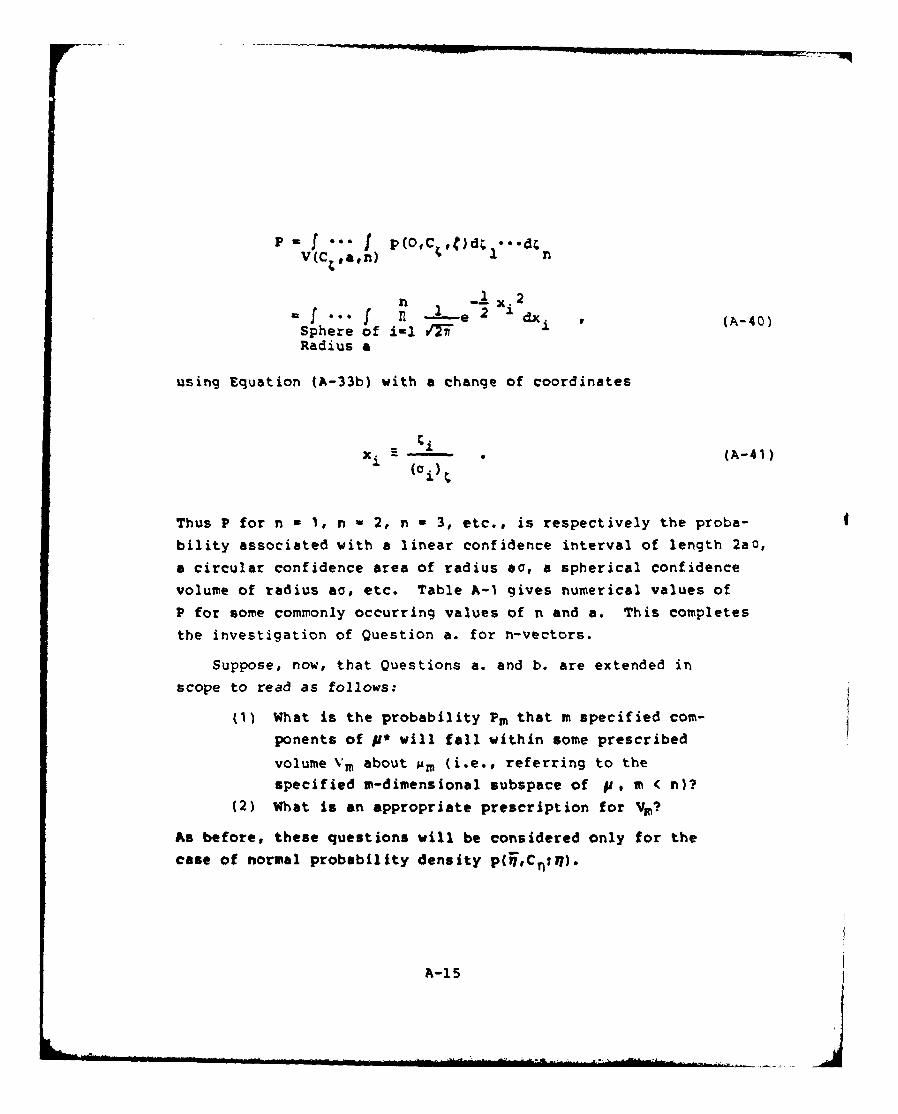
P f**Jp(OC4,t)d;,Lweed;V(C fan) n

-n x. 2

11 1' f I e 2 dx (A-40)Sphere of i-n PITRadius a

using Equation (A-33b) with a change of coordinates

Xi = ---- (A-41 )

Thus P for n * 1, n w 2, n - 3, etc., is respectively the proba-

bility associated with a linear confidence interval of length 2a0,

a circular confidence area of radius ao, a spherical confidence

volume of radius ac, etc. Table A-I gives numerical values of

P for some commonly occurring values of n and a. This completes

the investigation of Question a. for n-vectors.

Suppose, now, that Questions a. and b. are extended in

scope to read as follows:

(1) What is the probability Pm that m specified com-

ponents of pi* will fall within some prescribed

volume Vm about ym (i~e., referring to the

specified m-dimensional subspace of p, m 4 n)?(2) What is an appropriate prescription for VM?

As before, these questions will be considered only for the

case of normal probability density p(llCfl)1?).

A-15

o o q 0% OD N N CD 0% UAIA wD In m% in m C4 0 &M %D

q* 0r cc~ m 0 ' m 0 D NIA %Q fn 0% IA N1 N4 q' 0D I

en r- VN r- LM 0 qo 0 CIDr- co M w - 0 %0 r- in%Q %D oo 4 0 9- A iA It) 0W- f- C q % -ID M

0E-4

UJ-J M 0 % Ch m 0

.i~ D- IAm N 0D M~ - as IA %QCO L. v 0 C 0 0 0 w M

0~ ID I re N %0 0n w 0r Q

0

SOn OD C I- W MM- C IAOD N s ONMM 0 0 ~ I C C

0 0 % 0 C~ 0 0 0 CD C

toMOH

A-i16

To simplify the ensuing notation, assume for the moment

that the first m components of p* are those specified. Then

the probability density for the m components is

+W 4.m

P(1m ) - f. f p(TCi 171)dT)m+ .*dnn (A-42)

and

Pm - f f p(17m)dr,1 .drm (A-43)

The solution of the subspace problem then hinges upon a

fundamental theorem of multivariate normal probability. One

can prove that

1-1 f- 17. -1 IV1m

(Ym (2r) m~"2iC~ 1 C ~ n C (1 -

- P( C 111) (A-44)

Here the covariance matrix C m is the subset array of

Cr, corresponding to the m specified components of p*.

Since the forms of Equations (A-42) and (A-43) are iden-

tical to those of Equations (A-25) and (A-24), respectively,

all of the previous results for V and P of the full n-

vector immediately follow where one substitutes 17m and CTimfor V and C17 .

A-17

Extension to any m components of p* is obvious, since

the numbering of the components is arbitrary. One must, of

course, select corresponding components in forming 7 m and

Cnm-

Finally, up to this point the analysis has assumed that

both C n and T are known. If only 7 is known, however, one

can find p but not P. If only C is known, one can find P

but not P*. These comments also apply to m-fold subspaces

of these n-vectors.

L1

lk-18

BIBLIOGRAPHY

Abramowitz, M., and 1. A. Stegun, Handbook o6 atkematiedtFunctionh, U.S. Govmt. Printing Office, 1964.

Anderson, T. W., Intkoduction to Uuttivaiate StatihtitcAnaty~iA, John Wiley and Sons, New York, 1958.

Bell, W. W., Matkieea J0o SCitntiA4t and EngqieekA, VanNostrand Reinhold, New York, 1975.

Morrison, N., intkoducrton to Atquctiat Apoothimp andp~ediction, McGraw-Hill, New York, 1969.

A- 19

APPENDIX B

PROPAGATION ERROR MATRIX

THE PREDICTION

OF

SATELLITE EPHEMERIS ERRORS

AS THEY RESULT FROM

SURVEILLANCE-SYSTEM MEASUREMENT ERRORS

P&===Dm NO XAMK-m iIUM

APPENDIX B

PROPAGATION ERROR MATRIX

The first of the following subsections states the problem

of determining a matrix representing the error in the propa-

gation matrix [Equation (B-2)]. The second subsection gives the

solution approach and the solution itself. The final sub-section contains intermediate steps of the analysis.

1. The Propagation Error Matrix Problem

The objective here is to find the effect of error in the

state vector

x°o J (B-1)j

upon the propagation matrix

f 0 0 g0 00 f 0090

0 0 f 0 0 g4 ( * o , t , o ) ( 8 -2).,00o 00 (B-2)

00 0 0 [

Here (see Reference B-1)*

f - 1-± (1-cos Eu(B3af o (e-3a)

Equations (B-3a to 3d) are among Equations (7P18) and (7P19)with the convenient abbreviations p E Co, q E Do//&.Equations (5-4) to (B-6) are among Equations (7B5) - (7B9).Equation (3-8) is Equation (7P14)0 and Equation (B-9) isobtained by integrating Equation (4G4) with E E E-Eo andn lefined by Equation (4G7), identical with Equation (8-7)here.

B-3 esmm w- uiisma aGS AENNW

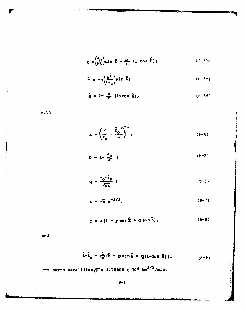
+r0 J . (1-005 E"' (B-3b)

a ~ E;(B-3c)

a2.Dn(r..--sin Z, (B-3c)

- 1- (1-cos )i (B-3d)

with

I -: (B-5)aa

foe roq - ; (B-6)

n /'i a'3/ 2. (B-7)

p al - p IoE + q sinE), (B-B)

and

A M 1 e

t-t o - pains * q K-cos E)J. (-9)

For Earth satellltea/1-x 3.78808 x 104 km 3/2 /min.

B-4

FJ

Specifically, the problem is to obtain an explicit repre-

sentation for *ttO , the p'opagation e44o4 matrix, as defined

by

*+ ." "o "*% 6 x . (B -1O )tt 0 tt 0

2. Solution Summary and Results

Using Equations (B-i) and (B-2), the lefthand side of

Equation (B-10) is

[ r61+ :J- o(L6o+-M 6o ;o ,(B- 1l) 0'6 0 ao L 0 0 , 0

where

the quantities xo , Yo, zo being the components of ro; etc.

Comparing the Equations (B-11) and (B-l0),

. 0 [a oJ I + °c o o

4. W , , _- _ 0

L °L o a " o o0 ;o C

B-5

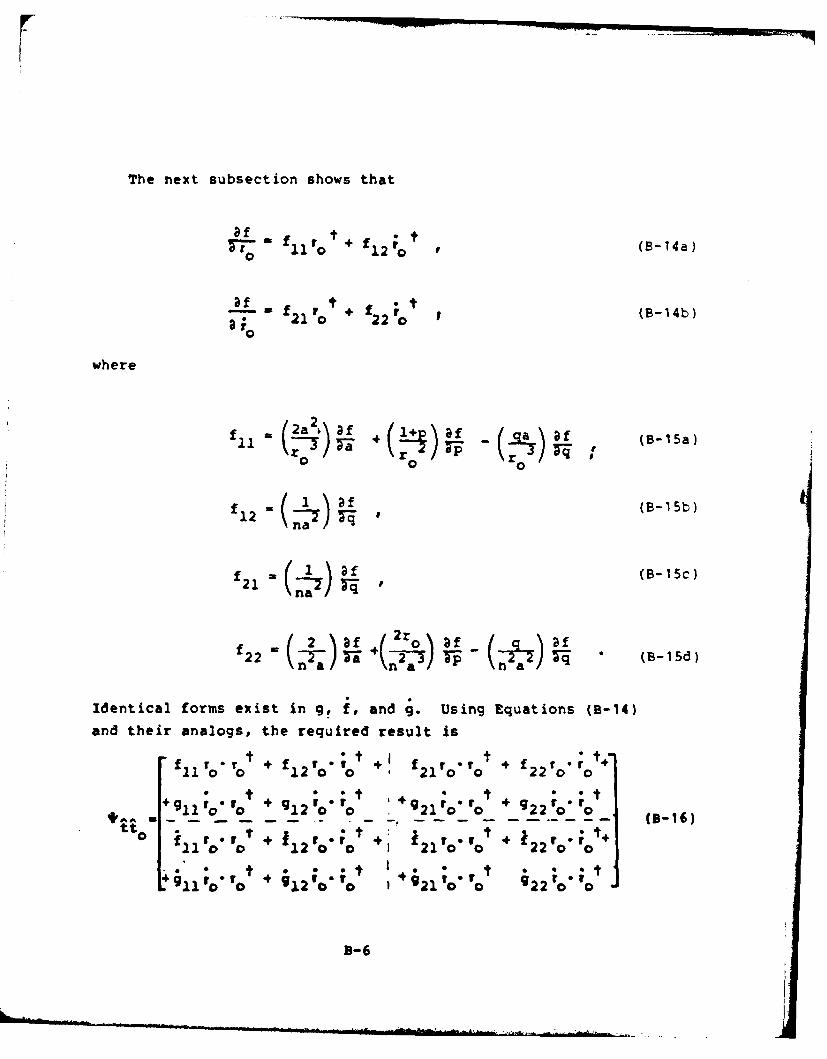
The next subsection shows that

af *1f 11 r0 + f 2r , (B-14a)0

7o f2 * r +f rO (B-14b)To 21 0 22 o

where

f 2a~ 2 t &t (f1+ I af(-

fa- f (B-15c)

f 2~ af +( 2r0 at f22 -2 q ~ (B-15d)

Identical forms exist in g, f, and g. Using Equations (B-14)

and their analogs, the required result is

f Ir " ,o' t + fr t- ; I + ro + o f f t;

1fi '0 0 12'o'o 21 0 0 22 0 0* ; .Set ;ot t+ .9 12%T ;o rt+912 'r - 0 t + 2 1 ;rotr + 922 o 0 0 B-

tt 0r0 + ~ 1 r 0 t + r rt + roo t+0 2a1 21 06 0 2200

• " , *i2l ;o" r " 'i22 ";o91 .1 r' 0 912r.& 0g1 0

B-6

The partial derivatives of Equations (B-15) and of its

analogs in g, f, and g are given in Table B-I, wherein:

E a* ~ - t )(B-i 7a)

ED S ". sin E (B-17b)

5 A

E - -(lcos E); (B-17c)

w B p gin i + q cosE . (B-18)

Note that expressions for the derivatives of f, g, f,

and g, with respect to each of the components of ro and

ro , are available in Reference B-2. There, development of

derivatives proceeds from expressions of the general form

of Equations (B-14) and (B-15) here, except that the

intermediate variables Do,rO , and 1/a are used

rather than p, q, and a. One can prove that the results

here are identical to those of Reference B-2, after cor-

recting certain misprints in the latter.*

3. Derivation of Partial Derivatives

This subsection contains derivations of Equations (B-14),

(B-15), and results of Table B-i with defining Equations

(B-17) and (B-18).

amA

' In Reference B-2, Equation (15C20), the term Ta has beenomitted (see Equation (15C5)). In Equatin (15C53) for4 r, the first denominator should read rora rather than

ro3.

B-?

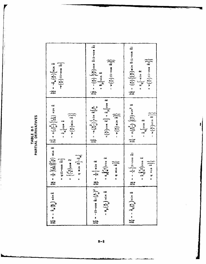
U0

00

a... 4 S Ua .4 U

W0 U 0

*J ., II ** wi

013 0 ol

UJI LU'U54 a.. 111ICA k.

m O ' t*

CL*

I - -la oW )4 - o

N~jp L~i~J ;;; _ S 5 5*

A. .

.4W -,31-01 0 (3

0w f9 0

B-8

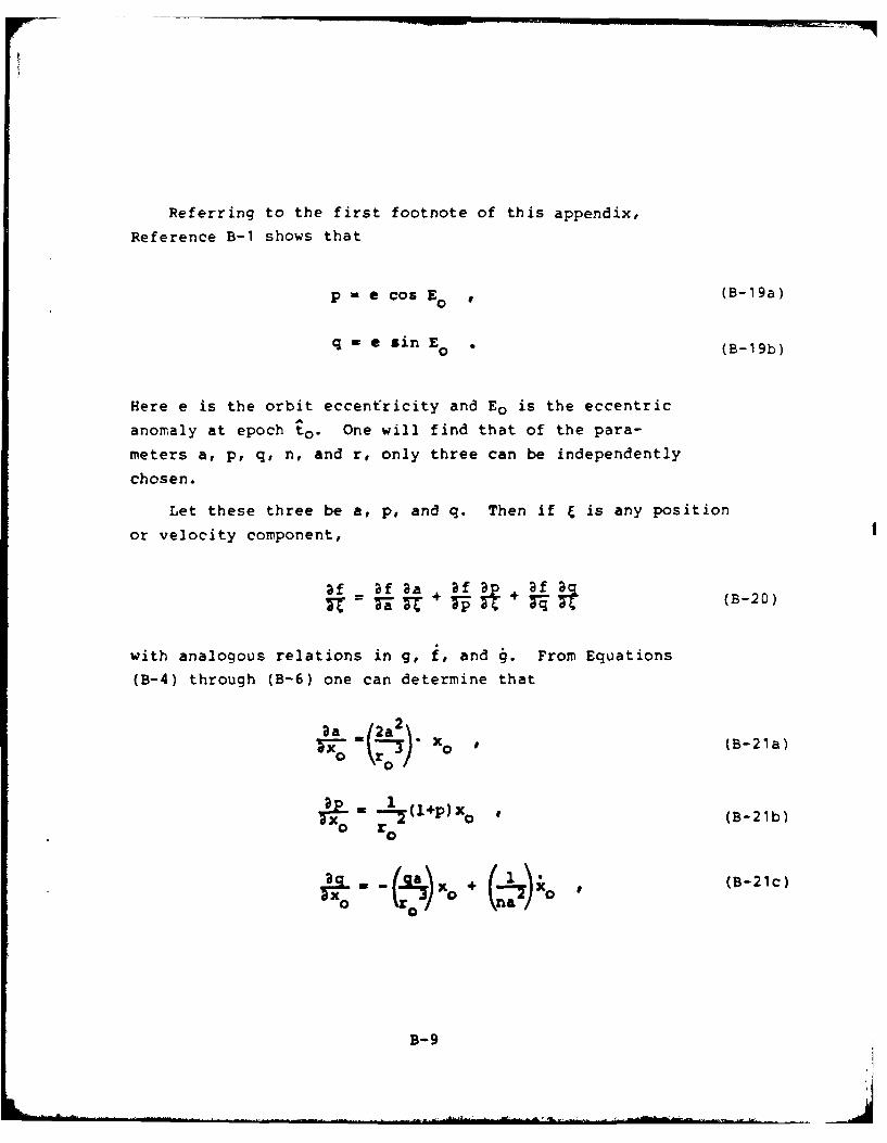
Referring to the first footnote of this appendix,

Reference B-i shows that

p - e Cos E0 , (B-19a)

q - sin E . (B-19b)

Here e is the orbit eccentricity and Eo is the eccentric

anomaly at epoch to. One will find that of the para-

meters a, p, q, n, and r, only three can be independently

chosen.

Let these three be a, p, and q. Then if & is any position

or velocity component,

= f f Bf(B-20)

with analogous relations in g, f, and g. From Equations

(B-4) through (B-6) one can determine that

aa t/2a2 \.

0 - )X (B-21a)0

=XO"EO-(l+P)xo ' (B-21b)

a (B-21b)o

B-9

Jl~

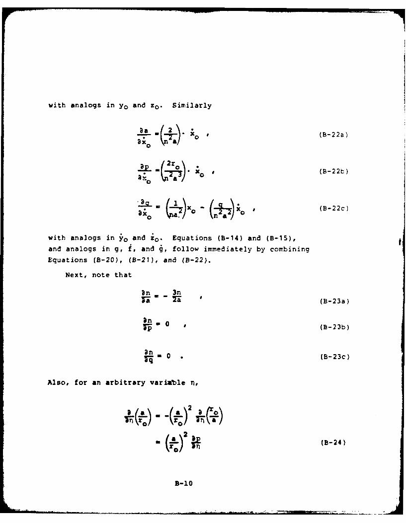
with analogs in yo and zo . Similarly

- (2\. -

a a

~ 2ro\-- O (B-22b)

a0

=70 x ;O (B-22c)

with analogs in yo and Zo. Equations (B-14) and (B-15),

and analogs in g, f, and j, follow immediately by combining

Equations (B-20), (B-21), and (B-22).

Next, note that

an 3n

Ta' =- 7-a(B-23a)

an- 0 (B-23b)

an- 0 (B-23c)

Also, for an arbitrary variable n,

_ _.L)2 ~

(a)'r)_ (B-24)

B-10

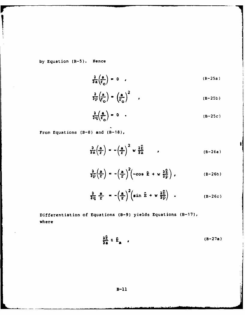
by Equation (B-5). Hence

0 ((B-25a)- r 0 ,

ap (B-25b)

T-q 0(B-25c)

From Equations (B-8) and (B-18),

3 2a - - ,(B-26a)

a - -Cos +• w (B-26b)

"r" - -in E + w TO (B-26c)

Differentiation of Equations (B-9) yields Equations (B-17),

where

3E (B-27a)B- Ea

B-11

T-P P(B-27b)

rq- lq(B-27c)

With the aid of Equations (B-23), (B-25), and (B-26) one

can then differentiate Equations (B-3) with respect to a, p,

and q to obtain the results in Table B-1.

5-12

REFERENCES

B-1. Herrick, S., Azt'~odynoam*.ez Vot. 1, Van Nostrand Reinhold,London, 1971.

B-2. Herrick, S., Azt odynamnich&, Vot. 2, Van Nostrand Reinhold,London, 1972, pp. 51-55.

B-13

APPENDIX C

INVERSION OF A MATRIX

THE PREDICTION

OF

SATELLITE EPHEMERIS ERRORS

AS THEY RESULT FROM

SURVE:LLANCE-SYSTEM MEASUREMENT ERRORS

nine

APPENDIX C

INVERSION OF A MATRIX

Suppose a matrix has the form

GH H G NH H H

H ... H H GHi(C- HH ... . %-i H H

LH a H H +i

wherein the GI , I=1,2,...,N, and H are themselves n X n

diagonal matrices with elements, for i=1,2...,n:

(G) ) 0 , (C-2)

(C-3)

The problem here is to find C- 1 , and concomitantly to

demonstrate that Equations (C-2) and (C-3) ensure its

existencei

The ensuing solution rests upon a generalization of

Cramer's Rule (Reference C-i. p. 286). Given a matrix

whose partitions are members of a field, the determinant of

the matrix is also a member of the field and can be evaluated

C-3 PiOUw - .A.SO 1

by standard manipulative techniques. Cramer's Rule thenholds for finding the inverse matrix, whose corresponding

partitions will again be members of the field.

Now, the set of n z n invertible, diagonal matrices plugthe null matrix, forms a field under matrix addition and multi-plication. Both GI and H are members of this field, assumingfor the moment that B as well as GI is invertible. Thus

Ici • (C1)z. 1A1Iz I 1,. M 1,2,...,1N (C-4)

an n X n matrix equation wherein all quantities are to be ex-pressed in terms of GI and H. Here ICI is the determinantof C. The quantity JA1 o is the cofactor of C3 1 , and (C'I)1 jis the general element of C-I.

One may use a recursive approach to evaluate the deter-minant IC1. Let

CN SC . (C-5)

Then

C1 G G1 + H

and for N>1 let CN_ 1 be the matrix of the first N-I rows andcolumns of CN .

Now one may expand ICNI via the last row, and after somerearrangement of rows and columns obtain the following:

C-4

G,4H ... H H H

1

-H H 00 St_3

H 0 0 0

-H H *.. % 3H H H

GjH H H H

H 0 H H H

G4H ... H H Ht10

-OH H *.. GN_ 34I H H

13 *.. %_H H

I: G2 *I .. H H0

* S S 5

One may evaluate the determinants here by subtracting thelast row from each of the other rows and then expanding viathe last column. Equation (C-6) then becomes

Ic NI Gm (GC-N NiNC +G O )ICI + H G( 1 G-1 (C-7)

Bv evaluatino IC21 and then IC31, one may infer that ICNI

probably has the form

1%I R fG 1 ~ + H I G 1\IiI-i /(C-EB

One may easily prove this result, for N>1, by substitution

into Equation (C-7).

Clearly ICNI is n z n diagonal, and

IC N I r •G i[ + Hii 1 i/G )i) C9

By Equations (C-2) and (C-3), none of the ICNIii vanishes,

so that JCN I' exists. Hence by Equation (C-4) all of the

C13"1 exist and so C"I exists.

Now in general [AI6j is an (N-1) x (N-1) matrix.

Define

I6aJ . 16j, (C-1o)

C-6

where for consistency of the preceding results

IaJii0 1 1 (C-1 1)

the n x n identity matrix. The values of iLzjll, corresponding

to N=2, are clearly

- G2 + H ; LA21 -- H2 1

1A211 22-Hi 1A2 1 = + H1 1

For N>2, one can find ILIJIN_1 by again using a recursion

approach. For the cases I=J, one may find IJAIIN_1 via

exactly the approach used previously for ICNI:

B~i +N N GN-I G I G=1 I (C-12)

Observe that this result holds for N>1.

For It(J, a typical 1AIJ IN-I for large N is

IAN_2,.31 .- H-1-1-1' ... 3+ H H 1C-13)

H --. H H H

H •. • H l H G4H

C- G+H

C-7

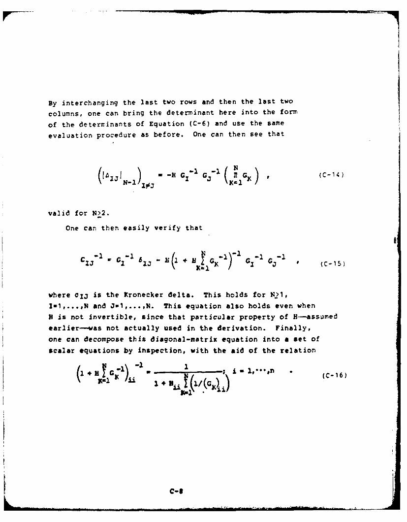
By interchanging the last two rows and then the last two

columns, one can bring the determinant here into the form

of the deterrinants of Equation (C-6) and use the same

evaluation procedure as before. One can then see that

- )- G ('GC)

valid for N>2.

One can then easily verify thatI

cx 3 l +IX) GI-1 Gj "1 (C-15)

where 0lj is the Kronecker delta. This holds for _>1,

1-1,...,N and 3-1,...,N. This equation also holds even when

B is not invertible, since that particular property of H-assumed

earlier--was not actually used in the derivation. Finally,

one can decompose this diagonal-matrix equation into a set of

scalar equations by inspection, with the aid of the relation

1- Y G 1 1 C 6

I

C-S i

RE FERENCES

C-1. G. Birkhoff and S. MacLane, A Suiivey ci Mode'tM Atgeba,MptcMillan, N.Y., 1965.

C-9

APPENDIX D

PRIMARY DISTRIBUTION LIST

THE PREDICTION

OFSATELLITE EPHEMERIS ERRORS

AS THEY RESULT FROM

SURVEILLANCE-SYSTEM MEASUREMENT ERRORS

pkamumphga UK.m? 11ui

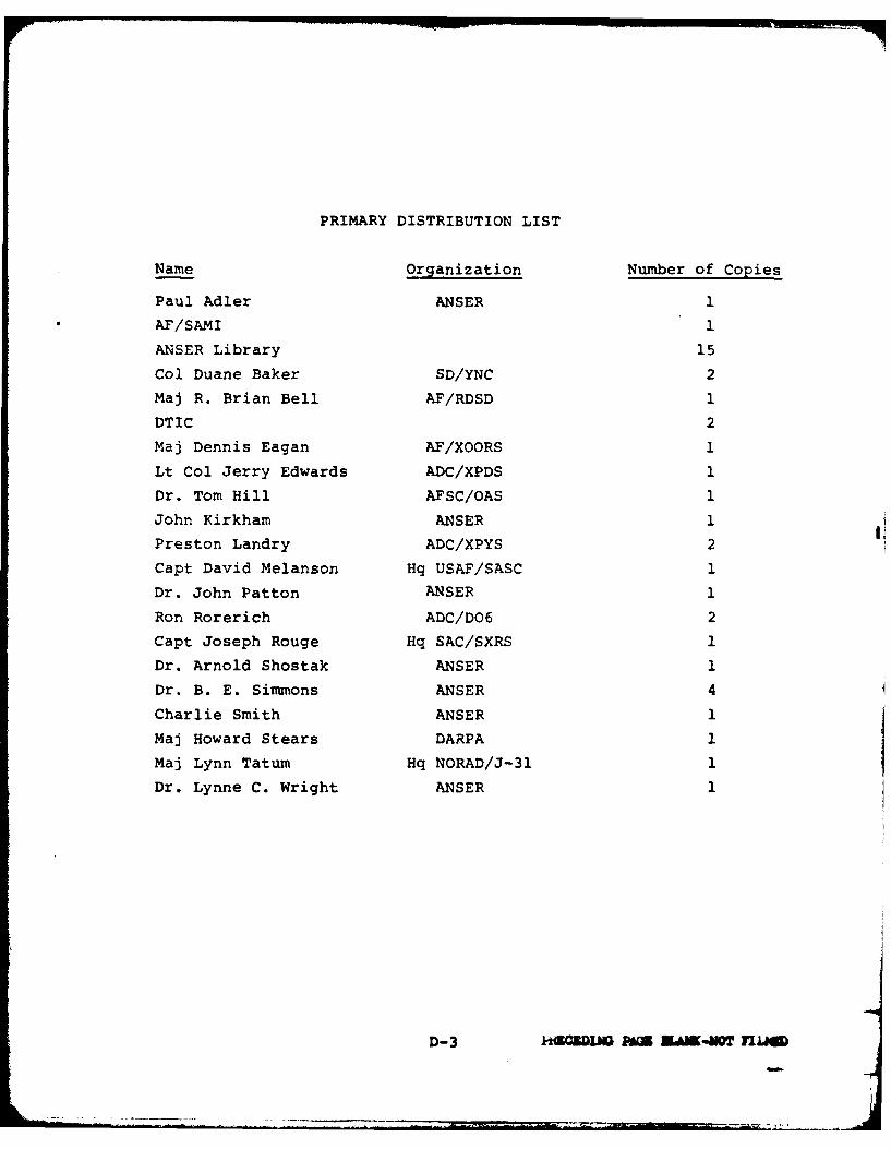
PRIMARY DISTRIBUTION LIST

Name Organization Number of Copies

Paul Adler ANSER 1

AF/SAMI 1

ANSER Library 15

Col Duane Baker SD/YNC 2Maj R. Brian Bell AF/RDSD 1

DTIC 2

Maj Dennis Eagan AF/XOORS 1

Lt Col Jerry Edwards ADC/XPDS 1

Dr. Tom Hill AFSC/OAS 1

John Kirkham ANSER 1Preston Landry ADC/XPYS 2

Capt David Melanson Hq USAF/SASC 1

Dr. John Patton ANSER 1

Ron Rorerich ADC/D06 2

Capt Joseph Rouge Hq SAC/SXRS 1

Dr. Arnold Shostak ANSER 1

Dr. B. E. Simmons ANSER 4

Charlie Smith ANSER 1

Maj Howard Stears DARPA 1

Maj Lynn Tatum Hq NORAD/J-31 1

Dr. Lynne C. Wright ANSER 1

D-3 kik cmZ no uIM-MTnu-m

UNCLASSIFIEDSECURITY CLASSIFICATION OF THIS PAGE (",en Date Entered)

REPORT DOCUMENTATION PAGE B RE COMPLETIOR

I. REPORT NUMBER 2 GOVT ACCESSION NO. 3 RECIPIENT'S CATALOG NUMBER

SpDN 80-4

4 TITLE (and Subllt) S. TYPE OF AEPORT A PERIOD COVERED

The Prediction of Satellite Ephemeris Errors Division Note

6. PERFORMING ORG. REPORT NUMBER

SpDN 80-47. AUTNOR(&j S. CONTRACT OR GRANT NUMBER's)

Dr. B. E. Simmons F49620-77-C-0025

9. PERFORMING ORGANIZATION NAME AND ADDRESS 10. PROGRAM ELEMENT. PROJECT, TASK

Analytic Services Inc. (ANSER) AREA& WORK UNIT NUMBERS400 Army-Navy DriveArlington, Virginia 22202

11. CONTROLLING OFFICE NAME AND ADDRESS 12. REPORT DATE

Director of Space Systems and Command, Control £ August 1981Communications, DCS/Research, Development & 13. NUMBER OF PAGESAcquisition, Hq USAF, Washington, D.C. 20330 115

14 MONITORING AGENCY NAME & ADDRESS(if dilerent from Controlling Office) 15. SECURITY CLASS. (of this report)

UNCLASSIFIED15a. DECLASSIFICATION DOWNGRADING

SCHEDULE

16. DISTRIBUTION STATEMENT (of this Report)

Approved for public release; distribution unlimited.

17. DISTRIRIr!ON STATEMENT (of the abetract entered In Block 20, if different from Report)

18. SUPPLEMENTARY NOTES

19. KEY WORDS (Continue on reverse aide Ilnecessary and identify by block number)

Earth Satellites Error EstimationSpace Surveillance Sensors Mathematical ModelSatellite Ephemerides

20. ASSZACT (Continue an reverse efde I neceeeory and Identify by block number)

This report derives equations predicting satellite ephemeris error asa function of measurement errors of space-surveillance sensors. Theseequations lend themselves to rapid computation with modest computer resources.They are applicable over prediction times such that measurement errors, rather

than uncevtaintise of atmospheric drag and of Earth shape, dominate In pro-ducing ephemeris error. This report describes the specialization of theseequations underlying the ANSER computer program, SEEM (Satellite Ephemeris

D on. 1473 cori, ,oil I. Nov., O5is0OL'T" ,DO 7JAN 7S UNCLASSIFIED

sSCuP1ITY CLASSIFICATION OF TNIS PAGE f(U9s Data £gtee)

' . .. i . .. '- :: - ... ... lib T-T :-'-'* -; ? : - '-- '-'-' - '- *' "| '- "' : - .. . .. El li ~ l "e 'H ,,,, ,,e

UNCLASSIFIEDIECUR I V CLASSIICATIOr1O THIS PAGEPIOrli D.o. Enterod)

20. (Continued) Error Model). The intent is that this report be of utilityto users of SEEM for Interpretive purposes, and to computer programmers whomay need a mathematical point of departure for limited generalization of SEEM.

UN~I A IF rSECUf1TrY CL ASSIVIC&?sOi OF ?1I PGIoeW DOMB nIeO.o)

k ..