Firm Investment with Liquidity Constraints:What Can the Euler Equations Tell us?1

Bronwyn H. HALLNuffield College, Oxford, UC Berkeley, IFS, and NBER

First Version: April 1991.This Version: February 1995

1This paper is drawn in part from an earlier paper entitled “R&D Investment at the Firm Level: Does theSource of Financing Matter?”, which was presented at the International Conference on Quantitative Economicsand Its Applications to Chinese Economic Development and Reform in the 1990s in June 1990 and the WinterMeetings of the Econometric Society in December 1990. I have benefitted from very helpful comments by StephenBond, R. Glenn Hubbard, Costas Meghir, Mark Schankerman, and seminar participants at the National Bureauof Economic Research, Stanford University, and the Institute for Fiscal Studies. They are of course absolvedof any responsibility for errors. I am also grateful to the National Science Foundation and the Committee onResearch, University of California, Berkeley, for support of the data preparation effort for this project, and toENSAE-CREST, Paris, (in particular, Jacques Mairesse and Christian Gourieroux) for their hospitality duringthe Winter and Spring of 1991.

1

1 Introduction

In previous papers (Hall 1992, 1991), I presented two kinds of evidence that both R&D and

ordinary investment were subject to liquidity constraints: first, increases in a firm’s debt level,

which reduces the amount of internal finance available to it, were followed by declines in invest-

ment. Second, instrumental variable estimates of a standard investment equation show that

correcting for simultaneity and firm-specific unobservables leaves only profits or cash flow as a

significant predictor of investment behavior; sales and Tobin’s q are no longer important. It

was also true that R&D assets were substantially less likely to have been financed by debt in

the past, which suggests that at least this source of external finance is relatively expensive for

R&D. None of these findings were based on estimates derived from a structural model of firm

behavior, which makes them difficult to interpret causally.

Several other researchers have used structural dynamic programming models of a firm mak-

ing investment and financing choices to test for the presence of and effect of liquidity constraints

on ordinary investment. For example, Bond et al (1990) have applied a model which is similar

to the one presented here to data on large U.K. firms and rejected the hypothesis that the Euler

equation for investment is the same for firms in all net worth positions. By and large, these re-

searchers have focused on the behavior of the Euler equation for the intertemporal substitution

of investment in the presence of liquidity constraints, with generally significant results. In this

paper, I develop such a model for firms which are investing in both ordinary capital and R&D

capital, and I investigate the extent to which we can learn anything from the Euler equation

estimates. The results are fragile and I explore the sources of this fragility of the estimates.

The results here are intended as a warning to those using this methodology with micro data.

2 The Modeling of Capital Structure and Investment

Once we admit that the financing and investment decisions of the firm may be interrelated, that

is, that the cost of different kinds of capital may vary by type of investment, we must face the

2

fact that forward-looking firms will choose their capital structure in such a way as to minimize

the longrun cost of capital for the investment paths they plan to pursue. For example, this

implies that we may observe correlation in the cross section between high debt-equity ratios and

low R&D expenditure, without that necessarily implying a one way causal relationship (capital

structure to R&D). In this case, we might instead be interested in sorting out the effects of an

exogenous change in the price of debt relative to equity on the incentives for R&D spending.

Discuss motivation for structural model.

I begin with a dynamic programming model of the firm’s investment problem which incor-

porates three types of financing for two kinds of investment: retained earnings, debt, and new

equity are used to finance investment in physical assets and in R&D capital. My presentation

here follows the work of Auerbach (1979), Poterba and Summers (1985), and Fazzari, Hubbard,

and Petersen (1988). More recent examples of this type of modeling are in Gilchrist (1990)

and Hubbard and Kashyap (1990). My model is different from most of the preceding work in

that it explicitly incorporates the stock of working capital, which has important implications

for the evolution of the cost of capital at the firm level. A major unsolved problem in the

development of any but the simplest dynamic programming models for investment is finding a

way to incorporate the measure of market value as a price and this problem remains unsolved

here, although I suggest an extended interpretation of Tobin’s q based on this model at the end

of the section. What the model does give us is a set of equations which describe the substitution

of investment across different time periods in response to changes in the cost of funds which

are induced by the liquidity position in which the firm finds itself.

I define the following variables:

c the tax rate on capital gains income

θ the tax rate on ordinary income

τ the corporate tax rate

Kt the capital stock at the beginning of period t2

2The dating of the stocks as beginning of period (implying that capital purchased this period does not

3

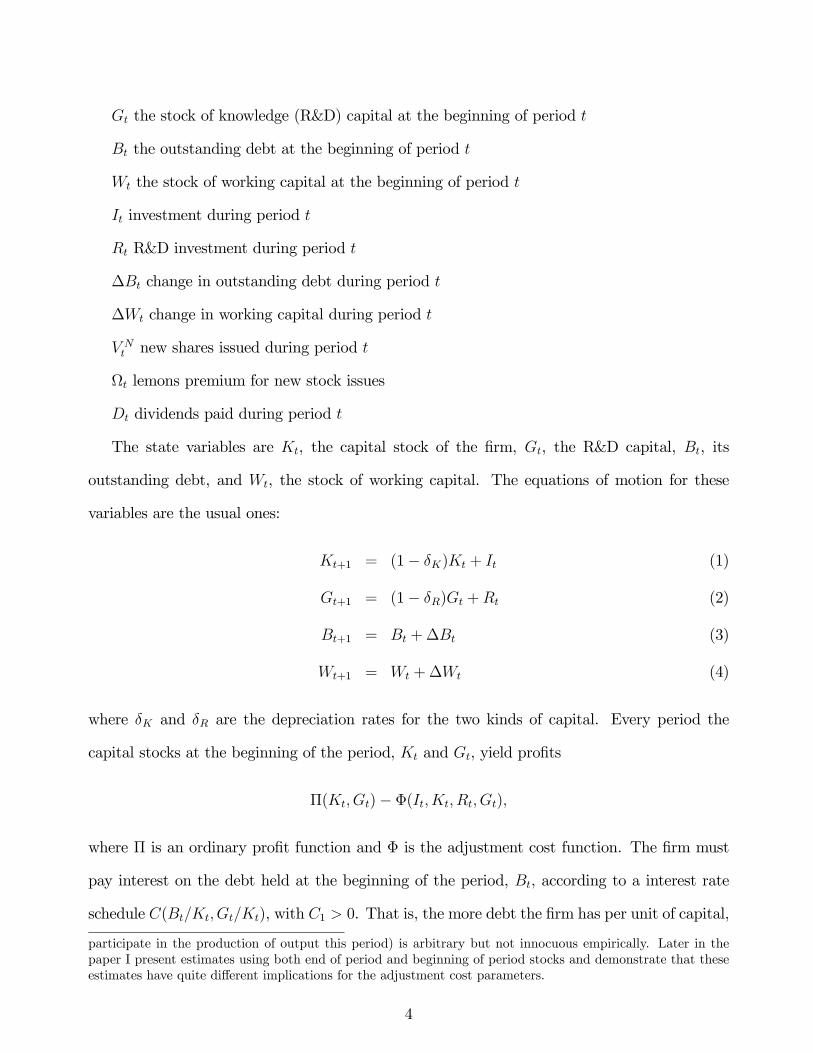
Gt the stock of knowledge (R&D) capital at the beginning of period t

Bt the outstanding debt at the beginning of period t

Wt the stock of working capital at the beginning of period t

It investment during period t

Rt R&D investment during period t

∆Bt change in outstanding debt during period t

∆Wt change in working capital during period t

V Nt new shares issued during period t

Ωt lemons premium for new stock issues

Dt dividends paid during period t

The state variables are Kt, the capital stock of the firm, Gt, the R&D capital, Bt, its

outstanding debt, and Wt, the stock of working capital. The equations of motion for these

variables are the usual ones:

Kt+1 = (1− δK)Kt + It (1)

Gt+1 = (1− δR)Gt +Rt (2)

Bt+1 = Bt +∆Bt (3)

Wt+1 = Wt +∆Wt (4)

where δK and δR are the depreciation rates for the two kinds of capital. Every period the

capital stocks at the beginning of the period, Kt and Gt, yield profits

Π(Kt, Gt)− Φ(It,Kt, Rt, Gt),

where Π is an ordinary profit function and Φ is the adjustment cost function. The firm must

pay interest on the debt held at the beginning of the period, Bt, according to a interest rate

schedule C(Bt/Kt, Gt/Kt), with C1 > 0. That is, the more debt the firm has per unit of capital,

participate in the production of output this period) is arbitrary but not innocuous empirically. Later in thepaper I present estimates using both end of period and beginning of period stocks and demonstrate that theseestimates have quite different implications for the adjustment cost parameters.

4

the higher the interest rate faced by the firm; the interest expense is fully deductible against

profits.

The firm’s problem is to maximize the present discounted stream of dividends by choosing

investment I and R, and financing sources V Nt , the new issue of equity, ∆Bt, the new issue

of debt, and ∆Wt, the change in cash reserves, subject to the capital and debt accumulation

constraints and the constraint that the dividends Dt be nonnegative:

Dt = (1− τ)[Π(Kt, Gt)− Φ(It, Kt, Rt, Gt)− C(Bt, Kt, Gt)−Rt] +∆Bt + V Nt

− ∆Wt − It ≥ 0 (5)

This equation assumes that the adjustment costs, interest costs and R&D expenditures are

expensed in the year in which they are made. It also assumes that the taxable portion of losses

is freely convertible into a source of financing for the firm’s new investment; that is, there is an

unlimited ability to carry losses forward.

The value of the firm to the present shareholders may then be expressed as the solution to

the following maximization problem:

MaxI,R,V N ,D,∆B,∆W

Et

∞Xs=0

(1 +ρ

1− c)−(t+s)

·(1− θ)

(1− c)Dt+s − (1 + Ωt+s)V

Nt+s

¸(6)

where ρ is the investor’s required after-tax rate of return. This maximization problem assumes

that when the shareholders issue new shares to the company, they must pay a premium in the

form of a decrease in value of their existing shares, because of the existence of lemons in the

equity market (Akerlof 1970, Fazzari, Hubbard, and Petersen 1988).3 It has also been assumed

that the shareholders are subject to dividend taxation and the taxation of realized capital gains,

as suggested by the work of Poterba and Summers (1985).

This maximization is to be done subject to the six constraints implied by equations (1), (2),

(3), (4), and (5) (two constraints) with associated Lagrange multipliers λKt , λRt , ξ

Bt , ξ

Wt , αt and

3Obviously the value of this premium is determined in equilibrium as a consequence of the nature of theprojects available and the taste and risk characteristics of shareholders and entrepreneurs. I am abstractingfrom this aspect of the model and simply assuming that the new shares must be sold at a discount, which mayvary over time but which is the same for all firms (since investors cannot tell good firms from bad). Later it maybe possible to allow this premium to depend in addition on the R&D intensity of the project being financed.

5

µt. I add two inequality constraints: one which prevents the firm from buying back all of its

own shares during some period, and one which forces the firm to keep a small positive stock of

working capital at all times.

V Nt > V where V < 0 (7)

Wt > W where W > 0 (8)

The Lagrange multipliers associated with these constraints are ηt and ηWt . This completes the

statement of the problem.

The first order conditions for the six control variables It, Rt,∆Bt,∆Wt, Dt, and V NT are the

following:4

λKt − αt[(1− τ)ΦI + 1] = 0 (9)

λRt − αt(1− τ)[ΦR + 1] = 0 (10)

αt − ξBt = 0 (11)

αt − ξWt = 0 (12)

αt − µt = (1− θ)/(1− c) and µtDt = 0 (13)

αt + ηt = (1 + Ωt) and ηt(Vt − V ) = 0 (14)

The first order conditions for the state variables Kt, Gt, Bt , and Wt are (after eliminating

λKt , λRt , ξ

Bt , and ξWt using equations (11), (12), (13), and (14)):

[ΠK(t)− ΦK(t)− CK(t)] = (1 +ρ

(1− c))αt−1αt[(1− τ)−1 + ΦI(t− 1)]− (1− δK)[1− τ)−1 + ΦI(t)](15)

[ΠG(t)− ΦG(t)− CG(t)] = (1 +ρ

(1− c))αt−1αt[(1 + ΦR(t− 1)]− (1− δR)[1− ΦR(t)] (16)

1 + (1− τ)CB(t) = (1 +ρ

(1− c))αt−1αt

(17)

ηWt = αt − (1 + ρ

(1− c))αt−1 and ηWt (Wt −W ) = 0 (18)

4The following presentation solves the model under certainty. Since the equations are mostly linear, it isstraightforward to add uncertainty later. The quantities which are in the information set at time t are ρ, thetax rates c, θ, and τ , the equity premium Ωt, and Kt, Gt, Bt, Wt, and Wt, along with the history of investmentand financing choices for the firm.

6

where I have compressed the arguments of ΠK,ΠG,ΦK,ΦG, CK, CG , and CB into the single

date t or t − 1 in order to save space. Equations (??) and (16) express the tradeoff betweeninvesting at time t− 1 and reaping the associated profits at time t, or waiting until time t tomake the equivalent investment, leaving the capital stock of the firm unchanged in periods t+1

and later. The pre-tax marginal profit from the additional unit of capital at time t is equal

to the difference in the costs of investment made at time t− 1 and investment made at time t(adjusted for the investor’s required rate of return and for any change in the shadow price of

the flow of funds constraint between the two periods).5

Equation (17) shows that the firm borrows to the point where the after-tax cost of borrowing

is equal to the investor’s required rate of return adjusted for the shadow price of the flow of

funds constraint. Because of the convexity and concavity assumptions on Π(.)and C(.), these

four equations together with the accumulation constraints (1), (2), (3), and (4) and the levels of

lagged investment It−1 andRt−1 will uniquely determineKt, Gt, Bt,Wt, It, Rt and∆Bt, provided

we knew the (endogenous) shadow prices αt−1 and αt. Note that this model will not uniquely

determine Dt and ∆Wt, but only their sum.

Before discussing the possible estimation strategies with which I might approach the em-

pirical model implied by equations (??)-(18), I analyze the implications of the model for the

cost of investment (my analysis does not differ in essentials from that of Poterba and Summers

(1985) and Fazzari, Hubbard, and Petersen (1988), but the addition of working capital does

affect some of the conclusions). I consider three cases (regimes): 1) µt = 0, ηt > 0 — no dividend

constraint and at the share repurchase maximum, 2) µt > 0, µt > 0 — at the dividend constraint,

but no new share issues, and 3) µt > 0, ηt = 0 — at the dividend constraint and issuing new

shares for additional financing. Poterba and Summers demonstrated that the fourth possibility,

5In equations (??) and (16) the corporate tax rate appears only once, as an increase in the price of ordinaryinvestment; this increase occurs because such investment is not expensed. This oversimplification of the differ-ence in tax policy for the two types of investment does little damage to the specification of the Euler equationssince the term (1 − τ) will appear only in the constant term and τ could be presumed to somewhat lowerthan the statutory rate to accommodate the investment tax credit, etc. However, it must be recognized thatinvestment has intertemporal consequences for the availability of future depreciation deductions and thereforehas an impact on αt; this has been ignored here.

7

a firm not constrained by dividends but issuing new shares, will never occur if the tax rate on

ordinary income exceeds that on capital gains.6 (This is also obvious from inspection of the

first order conditions.)7 My analysis of the first and third possibilities follows theirs closely,

while the second becomes a non-empty possibility in the presence of an ability to borrow: the

firm can finance new investment by taking on more debt rather than issuing new shares.

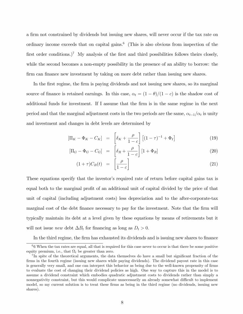
In the first regime, the firm is paying dividends and not issuing new shares, so its marginal

source of finance is retained earnings. In this case, αt = (1− θ)/(1− c) is the shadow cost of

additional funds for investment. If I assume that the firm is in the same regime in the next

period and that the marginal adjustment costs in the two periods are the same, αt−1/αt is unity

and investment and changes in debt levels are determined by

[ΠK − ΦK − CK] =

·δK +

ρ

1− c

¸ £(1− τ)−1 + ΦI

¤(19)

[ΠG − ΦG − CG] =

·δR +

ρ

1− c

¸[1 + ΦR] (20)

(1 + τ)CB(t) =

·ρ

1− c

¸(21)

These equations specify that the investor’s required rate of return before capital gains tax is

equal both to the marginal profit of an additional unit of capital divided by the price of that

unit of capital (including adjustment costs) less depreciation and to the after-corporate-tax

marginal cost of the debt finance necessary to pay for the investment. Note that the firm will

typically maintain its debt at a level given by these equations by means of retirements but it

will not issue new debt ∆Bt for financing as long as Dt > 0.

In the third regime, the firm has exhausted its dividends and is issuing new shares to finance

66 When the tax rates are equal, all that is required for this case never to occur is that there be some positiveequity premium, i.e., that Ωt be greater than zero.

7In spite of the theoretical arguments, the data themselves do have a small but significant fraction of thefirms in the fourth regime (issuing new shares while paying dividends). The dividend payout rate in this caseis generally very small, and one can interpret this behavior as being due to the well-known propensity of firmsto evaluate the cost of changing their dividend policies as high. One way to capture this in the model is toassume a dividend constraint which embodies quadratic adjustment costs to dividends rather than simply anonnegativity constraint, but this would complicate unnecessarily an already somewhat difficult to implementmodel, so my current solution is to treat these firms as being in the third regime (no dividends, issuing newshares).

8

investment. In this case, the marginal shadow cost of new funds for investment is (1+Ωt) since

the firm must pay the new shareholders a premium in order to induce them to purchase the

equity. In the first regime the shadow cost is less than unity, since the tax rate on the capital

gains is less than that on ordinary income,8 while in the third it is greater than one. In the words

of King (1987), equity is “trapped” within the firm, since it pays to undertake investments with

retained earnings which would not be undertaken if new equity has to be issued. This is not

a novel point (King 1986, 1987; Auerbach 1984), but it is important to the argument of this

paper.

Because I have assumed that the cost of debt is a well-behaved monotonic function, in either

regime 1 or regime 3 the firm may also be issuing (or retiring) debt (the shadow price of the

debt identity ξt is just equal to the negative of the shadow price of the capital accumulation

or sources and uses of funds identity). Only in regime 2 is debt the marginal source of new

funds for investment: in this case dividends have been exhausted (Dt = 0 and µt > 0) while

new shares are still too highly priced (V Nt = 0 and ηt > 0). This is illustrated in Figure 1. In

this region, the firm will obtain funds for new investment either by retiring less debt (if ∆Bt is

negative) or by issuing more (when ∆Bt is positive). Without further knowledge of the cost of

debt function it is not possible to say which the firm will be doing.

What are the implications of this model for the data and the hypotheses I have suggested

in the introduction? First, it clearly indicates that liquidity constraints may be important for

both types of investment, since the shadow price of the flow of funds constraint (4) increases

when the marginal source of funds is debt or external equity. However, the tradeoff between

investments this period and those next period, which are what drive the Euler equations (14),

(??), and (16) are affected only if the firm is changing regimes between periods, or if it is in

regime 2 (no dividends and no new shares), where αt could differ from αt−1. In other words,

a firm paying dividends may face a lower cost of capital than one which is not, but we will

not necessarily learn this from the Euler equations. We will have to focus on firms changing

8At least until 1986 in the United States.

9

financing regimes in order to detect this fact, which weakens the power of the test.

Second, if R&D is more subject to asymmetric information problems and does not create

securable assets, there are several implications: the shadow price of the flow of funds constraint

should be higher for R&D-intensive firms both in regime 2 (because the cost of debt rises as

the share of capital in knowledge assets rises) and in regime 3 (because the lemons premium Ωt

is higher for R&D-intensive firms). In addition, when a firm shifts to a higher cost financing

regime (for new investment; the average cost of the firm’s financial structure per unit of capital

may have fallen) the desired level of debt will be lower than it would be for a non-R&D firm

and the real marginal profit of capital (adjusted for its true cost) will also be lower. However

a clear prediction as to the level of investment is not possible without knowing more about the

form of the profit function and the adjustment cost function.

Like Bond and Meghir (1990), who have pursued a parallel line of work using United King-

dom firm data, I have chosen to investigate investment under financial constraints using an

Euler equation approach since this approach requires slightly fewer assumptions on the model

(in particular, it does not require linear homogeneity of the profit function or strong financial

market efficiency). However, it is instructive to examine the efficient markets q-model interpre-

tation of this model under the assumption of linear homogeneity of the value function (which

would be implied by linear homogeneity of each of its components in an additively separable

model).9 To do this analysis, I simplify the value function by excluding the possibility of new

share finance. In this case, the three envelope conditions for the stocks Kt, Gt, and Bt are the

following:

Et∂V

δKt= Etαt

½(1− τ)

·∂Y

∂Kt

¸+ (1− δK)

¾(22)

Et∂V

δGt= Etαt

½(1− τ)

·∂Y

∂Gt+ (1− δR)

¸¾(23)

Et∂V

δBt= Etαt

½(1− τ)

·∂Y

∂Bt

¸− 1¾

(24)

9The following discussion relies in part on insights in Hayashi and Inoue (1990), although the interpretationof αt is new. See that paper for more complete statements of the model for investments in multiple capitalstocks under uncertainty and proofs.

10

where Yt = Πt−Φt−Ct is profits net of adjustment and interest costs and αt = µt+(1−θ/(1−c)as before.

If the value function is linear homogeneous in the (known) stocks Kt, Gt, and Bt,10 then

Euler’s theorem gives the following equilibrium relationship between the observed value of the

firm and its capital stocks:

Et[V (Kt, Gt, Bt)] = Etαt[(1− δK)Kt + (1− τ)(1− δR)Gt −Bt (25)

+(1− τ)[Π(Kt, Gt)− C(Bt,Kt, Gt)]

This equation says that in equilibrium the market value of the firm during period t is expected

to be the sum of terms arising from the stocks at the beginning of the period plus the profits

which are expected to be earned on them during the period, all discounted by the cost of the

flow of funds constraint to the firm. The quantity αt (which is not a parameter, but a variable

under control of the firm) plays a key role in this relationship and can be interpreted as a

kind of Tobin’s q: when the firm is paying dividends and obtaining new funds for investment

from retained earnings, αt is low, signaling that equity is “trapped” within the firm and that

low quality investments are being made (on the margin). When αt is above one, the firm is

“liquidity constrained” and faces good investment opportunities on which it is unable to act.

In passing, I note that we would not expect αts substantially less than one to persist in

equilibrium: the q model of investment relies heavily on adjustment costs to prevent firms from

bringing q back to unity immediately, and this property also exists for my model. In practice,

the type of firm which is characterized by αt less than one and poor investment opportunities

corresponds to one of Jensen’s (1986) firms which have “free cash flow” and are subject to

breakup or restructuring in order to increase αt. This model, with its smoothly increasing

adjustment costs, does not envision such a solution.

Although I have not presented it here, I would conjecture that the solution to the problem

which includes new share issues has much the same character; because of the assumption of

10Rockinger and Restoy (1993).

11

linear homogeneity, it would effectively require all shares, not just the new shares, to be valued

at the premium αt = (1 + Ωt). In this case, there would seem to be no way other than

improvements in information to reduce the lemons’ premium and bring the αt of firms back to

unity. On the other hand, the fact that new share issues tend not to occur every year suggests

that firms rarely have high value investment opportunities present themselves year after year.

Equation (25) suggests an alterative way to approach the investigation of the existence of

liquidity constraints, which I pursue in other work (Hall 1990c). A finding that equation (25)

did not differ substantially across dividend-paying and non-dividend-paying firms would reject

the model presented here (although the converse finding could have several interpretations).

I have chosen here to focus my empirical investigation on the Euler equations for investment

and R&D investment, since this test does not require the imposition of market efficiency to be

implemented.

3 Estimation of the Structural Model

In this section of the paper, I use the model of Section 2 to develop tests of the impact of

liquidity constraints or financial structure on investment. The most difficult parts of the task

are identifying sets of firms which are liquidity constrained and choosing appropriate functional

forms for the marginal product of capital and the cost of debt finance. I begin with the second

problem, which arises even in an ordinary investment model with no liquidity constraints.

Economic theory provides relatively little guidance for the exact form of the marginal profit

from a unit of capital and the marginal cost of a unit of debt; I have chosen to estimate the

simplest model which is capable of incorporating the features of oligopolistic competition which

I believe to be important. These are the possibility of non-constant returns to scale in capital

and the variable input factors and the existence of some degree of market power (a finite demand

elasticity). Thus I assume a Cobb-Douglas production function with capital coefficients β and

γ, a coefficient for labor and variable factors α, and scale coefficient s = 1 − β − γ − α (so

12

that s = 0 corresponds to constant returns), and a constant-elasticity demand function with

demand elasticity ε = η(1 − η). Given stocks K and G, a profit-maximizing firm facing such

a production function and demand curve will choose variable inputs (labor and materials) and

output so that profits are proportional to powers of K and G, and thus to output Qt:

Π(Kt, Gt) ∼ [Kβt G

γt ]1/(η−α) ∼ Q

1/ηt (26)

Note that when α = 1−β−γ (constant returns) and η = 1 (perfect competition), profits arehomogeneous of degree one in K and G.11 If it were not for the fact that there are adjustment

costs to increasing and decreasing the capital stock which work through the associated financing

constraints (in particular, debt costs), the level of the capital stock would be indeterminate.12

This form of the profit function yields the following expressions for the marginal variable

profit from a unit of capital:

ΠK(t) ∼ Q1/ηt /Kt ΠG(t) ∼ Q

1/ηt /Gt (27)

For the adjustment cost function I used the conventional form which makes the costs of adjust-

ment per unit of investment a function of the rate of investment:

Φ(It, Rt,Kt, Gt) = φ0 + φKI2t /Kt + φRR

2t /Gt (28)

Obtaining a sensible cost of debt function proved more difficult: the function should be pro-

portional to debt and depend on the relative levels of the two capital stocks. I used the form

most frequently found in the liquidity constraint literature (see, for example, Bond and Meghir

11In fact, it is easy to show in this case that profits divided by the price coefficient times output is just equalto β, the capital coefficient, which is the well-known result that capital’s share equals its coefficient under CRSand competition.12For this case (perfect competition and CRS) one can show in the absence of debt financing that if the

after-corporate tax return to capital less depreciation is more than the investor’s pre-tax required rate of returnρ/(1 − c), the firm will wish to expand its capital at least to the point where dividends are exhausted; if thereturn to capital is large enough to cover the equity premium Ωt, the firm will wish to expand its capital stockinfinitely, using new share issues to finance the additional capital. Obviously a more realistic model would allowΩt to increase with the size of the new share issue to allow for some kind of diminishing returns or generalequilibrium considerations, but this detail is unimportant for the empirical work, since new share issues do tendto be bounded.

13

1990), which has the virtue of simplicity. Since the variables were rarely significant even in this

first order form, extensive experimentation did not seem warranted:

C(Bt,Kt, Gt) = [c0 + c1(Bt/Kt) + c2(Bt/Gt)]Bt (29)

All of the cis should be greater than zero.

The Euler equations (14) and (??) for the two capital stocks have the following form when

equations (26)-(29) are used to define the marginal profit of capital and the marginal cost of

debt:

Et−1

(ItKt- const -

Ã(1 + ρ

1−c)

(1− δK)

µαt−1αt

¶µIt−1Kt

¶− β/(η − α)

2φK(1− δK)

ÃQ1/ηt

Kt

!(30)

− 1

(1− δK)−µItKt

¶2− c12φK(1− δK)

µBt

Kt

¶2!)= 0

Et−1

(Rt

Gt- const -

Ã(1 + ρ

1−c)

(1− δR)

µαt−1αt

¶µRt−1Gt−1

¶− γ/(η − α)

2φR(1− δR)

ÃQ1/ηt

Gt

!(31)

− 1

(1− δR)−µRt

Gt

¶2− c22φR(1− δR)

µBt

Gt

¶2!)= 0

In the simple neo-classical world where the source of finance does not matter for investment,

these equations would be affected in two ways: the relationship between lagged and current

investment would not be mediated by αt−1/αt and the terms involving debt, Bt/Kt and Bt/Gt,

would not appear. Although it is easy to test for the latter effect, developing a method for

evaluating the importance of the change in the shadow cost of funds to the firm is far more

difficult. The approach taken in this paper is in the same vein as tests in several recent papers

( ); it focuses on the firms which undergo substantial changes in dividend policy or issue a

large number of new shares. Before discussing these tests, however, I begin by exploring the

specification of the Euler equation in the absence of liquidity constraints, that is, one where

αt−1/αt is unity for all firms.

In that case, except for the term involving output, these equations are linear in the variables

and can be estimated using two or three stage least squares with the investment rates as the

14

dependent variables and all of the variables in the information set at time t− 1 as instruments.Provided the covariance matrix is diagonal in the time dimension, the three stage least squares

estimates will be asymptotically efficient (and will coincide with the GMM estimator for this

problem). In order to save on computation time and avoid the difficulties of dealing with a

nonlinear estimation problem, I begin by setting η to unity and using a linear three stage least

squares estimator.13

Before I present the estimates of this structural model, one more potentially very important

problem with this approach needs to be discussed: the heterogeneity of the data sample to which

this model will be applied. The model assumes that the firms are completely described by the

variables included and that all other differences across firms are accounted for by differences

in their random outcomes which are not related to the past history of the firm. This is clearly

counter factual, but unavoidable. I make two attempts to mitigate the problem: the first

is that I confine my sample in this part of the paper to the so-called scientific sector, that is,

firms in the Chemicals (including Pharmaceuticals), Computing Equipment, Electric Machinery

and Electronics, Aircraft, and Scientific Instruments industries. This reduces the number of

observations to about 4500 for approximately 600 firms in an unbalanced panel for 1976 to

1987. The number of observations in each year before and after trimming is shown in Table

1.14 The result of this restriction should be to focus interest on firms for whom R&D is a

major part of their investment strategy. Firms in the scientific sector have a stock of knowledge

capital which is about one fifth that of ordinary capital on average, while for firms in the other

manufacturing sectors the share is much lower ( ) when it is measured.

The second attempt to control for heterogeneity is the usual one of adding unobserved

individual firm effects to the model and conditioning on them by differencing the regression.

This will control only for additive effects, leaving any multiplicative effects (such as differences

13For the form of the regression and timing of the capital stocks which I eventually settled on, preliminaryexperiments indicate that η is poorly identified, but clearly close to unity.14Since my model is in terms of ratio variables and quite sensitive to outliers, all observations with ratios

greater than about five times the interquartile range away from the median were removed before estimation.

15

in the marginal product of capital in the profit function) as potential sources of bias. As Bond

and Meghir (1990) have pointed out, the inclusion of fixed firm effects can also control for some

forms of sample selection and attrition bias. I present these estimates following those for the

basic set of Euler equations.

In Table 2 I show estimates of equations (30) and (31) which were obtained using three stage

least squares. The first question which arises when implementing a discrete-time investment

model with expectations is the exact timing of the variables, and this regression is no exception.

Two timing issues arise, both of which are explored in Table 2: the first is the choice of dates

for the instrumental variables (the information set) and the second is whether beginning or end

of period stocks should be used. The timing of the theoretical model described in section 3 of

the paper is that the stocks (capital, R&D capital, and debt) are dated at the beginning of

the period, while the flows occur during the period. Under the assumption that the dynamic

program is computed at the beginning of year t, the information set at t− 1 should include theflows during that period and the levels of the stocks at the end of the period. This means that

the lagged investment rate should be treated as predetermined in the estimation. Estimates

computed using these timing conventions are shown in column 1 of Table 2; they are the least

satisfactory of the estimates in this table.

There are several reasons why variables lagged once might not be appropriate instruments

for these regressions: first, they may not be completely known at the time investment plans

are made,15 and second, the random measurement error which occurs in such large data sets

can easily contaminate the orthogonality condition and bias the coefficient of lagged investment

downwards. In columns two and three, I present results obtained using instrument sets which

include variables lagged twice and three times, and then lagged only three times. These esti-

mates are fairly close, and, in the case of investment in physical capital it makes a considerable

difference to the estimates, which suggests some justification for my concern.

15In fact, these variables are generated in the production of the 10-K and Annual Reports for the firm, whichmake take place several months into the new fiscal year.

16

The Euler equations (30) and (31) have several implications, some of which are contradicted

strongly by the estimates in columns 1 through 3: first, the coefficient of the lagged investment

rate should be positive and greater than one, unless αt−1/αt is systematically much less than

one. This is not the case, in spite of my attempts to correct for measurement error. Second,

the coefficient of the output-capital ratio should be negative, which reflects the fact that in

periods when the productivity of capital is high, investment will be deferred in order to keep

the adjustment costs low, holding the previous investment rate constant. The coefficient of the

output-capital ratio is insignificantly different from zero for investment, it is robustly positive

for R&D (even under different specifications). Although the model says that when the output-

capital ratio is predicted to be high, the firm should compensate by planning a lower investment

rate to reduce adjustment costs, the data strongly suggest that liquidity considerations domi-

nate, in the sense that high sales implies more investment rather than less. Note that this is

not the result of news in sales acting as a proxy for surprises in expectations, because all of

these estimates are instrumental variables estimates based only on the movements which are

predictable from past investment and sales ratios.

A third implication of the model is that the coefficient of the investment rate squared should

be negative, because this represents the marginal cost of having a higher level of capital in the

profit function. Holding the profit rate constant, the higher the level of capital stock, the lower

the marginal adjustment cost due to capital and the higher should be the investment rate.

Although small, these coefficients are both positive and highly statistically significant.16

The model outlined in Section 3 of the paper makes the assumption that capital investment

undertaken this year does not become directly productive until next year; this is as arbitrary

16One problem here is that the model assumes that the investment rate can be positive or negative; if thedata came this way, it would be far less likely that the raw correlation of investment and investment squaredwould be nonzero; given that the rate is always positive, it is hardly surprising that the estimated coefficient ispositive (although in principle the Euler equation estimates could have given either sign). In this connection,note that if the measurement error in the investment rate is skewed to the right, as is likely, the coefficient ofthe investment rate squared will be biased upwards. This may account for the decline in the coefficient of theinvestment rate squared when it is instrumented or the data are trimmed (compare columns 1 or 3 of Table 5to column 2).

17

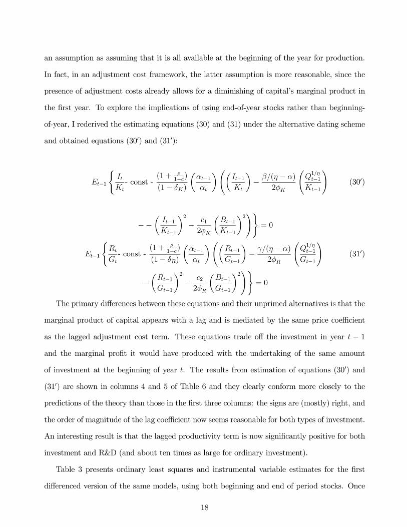
an assumption as assuming that it is all available at the beginning of the year for production.

In fact, in an adjustment cost framework, the latter assumption is more reasonable, since the

presence of adjustment costs already allows for a diminishing of capital’s marginal product in

the first year. To explore the implications of using end-of-year stocks rather than beginning-

of-year, I rederived the estimating equations (30) and (31) under the alternative dating scheme

and obtained equations (300) and (310):

Et−1

(ItKt- const -

(1 + ρ1−c)

(1− δK)

µαt−1αt

¶ÃµIt−1Kt

¶− β/(η − α)

2φK

ÃQ1/ηt−1

Kt−1

!(300)

−−µIt−1Kt−1

¶2− c12φK

µBt−1Kt−1

¶2!)= 0

Et−1

(Rt

Gt- const -

(1 + ρ1−c)

(1− δR)

µαt−1αt

¶ÃµRt−1Gt−1

¶− γ/(η − α)

2φR

ÃQ1/ηt−1

Gt−1

!(310)

−µRt−1Gt−1

¶2− c22φR

µBt−1Gt−1

¶2!)= 0

The primary differences between these equations and their unprimed alternatives is that the

marginal product of capital appears with a lag and is mediated by the same price coefficient

as the lagged adjustment cost term. These equations trade off the investment in year t − 1and the marginal profit it would have produced with the undertaking of the same amount

of investment at the beginning of year t. The results from estimation of equations (300) and

(310) are shown in columns 4 and 5 of Table 6 and they clearly conform more closely to the

predictions of the theory than those in the first three columns: the signs are (mostly) right, and

the order of magnitude of the lag coefficient now seems reasonable for both types of investment.

An interesting result is that the lagged productivity term is now significantly positive for both

investment and R&D (and about ten times as large for ordinary investment).

Table 3 presents ordinary least squares and instrumental variable estimates for the first

differenced version of the same models, using both beginning and end of period stocks. Once

18

again, the estimates for the model using end of period stocks and instrumental variables lagged

twice are by far the most reasonable for the adjustment cost parameters, although they are

now rather imprecisely determined. The interesting feature of these estimates is twofold: the

strength of the marginal profitability of capital term, which has increased tenfold, and the

(correct) negative sign of the debt term.

Based on the results in Tables 2 and 3, I have chosen to use the specification in column 4

of that table (end of year stocks and variables lagged twice and three times as instruments) as

the basis for my tests of the model with liquidity constraints. To construct a test, one needs to

know the value of αt−1/αt for different firms. Ideally I would like to parameterize this parameter

as a function of factors which affect the differences in the cost of funds between periods, but

I have already pushed the data almost as far as it will go, and a somewhat cruder test seems

appropriate here.

Recall from Figure 1 that dividend-paying firms are expected to have às below unity, while

firms which issue new shares during a period have às greater than one. This suggests that the

largest effects on αt−1/αt should be observed for firms which shift from paying to not paying

dividends (and vice versa) and firms which issue new shares one year and not the next. To

explore this idea, I divided the firms into three different groups in two ways: first, those which

stop paying dividends during a period (αt−1/αt < 1), those with no change in dividend policy

(αt−1/αt = 1), and those which start paying dividends during a period (αt−1/αt > 1). Second,

firms which issue new shares during a period (αt−1/αt < 1), those with no change in new share

issues (αt−1/αt = 1, and those which issued shares last period but not this (αt−1/αt > 1). I

then reestimated the model of column 4, Table 5 with the first and third groups of firms allowed

to have their own set of coefficients (by including a set of variables for these firms multiplied

by a dummy). An F-test can be used to test whether the coefficients of these two groups of

firm differ significantly from the sample as a whole.

The results are shown in Table 4. The first problem with this methodology is immediately

19

obvious: the fact that so few firms change their dividend payment policy from period to period

weakens the power of this test both by leaving few observations in the regime-changing category

and because the dividend policy is a poor indicator of liquidity due to its sluggishness. Although

the test for parameter constancy is accepted when dividends are used to define constrained

regimes, this may be simply because the sample is so small. When new shares are used to

define constrained regimes, the test for parameter constancy is rejected.

The model predicts that coefficients for the firms which move from a less constrained to

a more constrained position (as signaled by the cessation of dividends or the issuing of a

substantial block of new shares) should be lower in absolute value than the sample as a whole.

Although this appears to be true to a certain extent when the firm issues new shares, the

results for dividends are very weak and mostly of the wrong sign. The model also predicts

that firms which become less liquidity constrained (start paying dividends or issue new shares

in the previous period and not this one) in the current period should have coefficients higher

in absolute value than the sample as a whole. This is invariably not the case, except for the

output-capital ratio, which has the wrong sign to begin with. These firms are also the ones

primarily responsible for the rejection of parameter constancy. The strongest support for the

hypothesis that liquidity constraints impact on R&D investment is for the firms which issued

a substantial number of shares in the previous period and are now unconstrained: these firms

have an R&D investment rate which is 17 percentage points higher, other things equal (recall

that the overall average is 20 percent, so this represents a near doubling).

4 Conclusions and Extensions.

For the patient reader who has gotten this far, and not thrown up her hands in disgust and

walked away after seeing the estimation results in Table 4 (or perhaps even Table 2), I think a

number of things can be learned from the model and results presented here. First, I believe the

model helps greatly to clarify our thinking on the subject of financial factors for investment,

20

and for R&D in particular. It highlights the importance of the parameter αt, the shadow price

of the flow of funds constraint, which is a kind of cost of capital to the firm, both in determining

the level of investment (which is inversely proportional to αt), and in valuing the firm’s existing

capital stock (equation 25)). The model also makes it clear that the allocation of investment

from one year to the next is only affected by à when it changes over time and focuses our

attention on such regime shifts.

Second, I would hope the reader would come away from the paper with some skepticism

concerning reported estimation of Euler equation parameters with firm data. Table 6, in partic-

ular, demonstrates the sensitivity of the results to the exact timing of the model (note that this

is not because of incorrect timing of the information set considered). In addition, I would argue

that basing a test on the changes in investment behavior from one period to the next, although

theoretically sound, is inherently likely to run into problems of power due to the imprecision

with which many of the variables are measured and the heterogeneity of firm behavior, which

is magnified when year to year changes are considered. The quality of the information which

is being used relies on the individual firm’s ability to shift investment between periods in re-

sponse to small changes in the availability of funds and the marginal product of capital, and

such movements may be swamped by the variance of all the noise and unexpected shocks to

the firm’s profits and investment stream.

Third, in spite of the weakness and instability of the Euler equation estimates, I believe

we can learn something from them. The most robust finding in the various tables is that the

marginal product of capital enters positively for both investment and R&D, and was frequently

more important (or significant) for the latter. This is contrary to the precise predictions of

the structural model (which arise because the firm should be substituting away investment in a

period when the marginal productivity of capital is predicted to be high), but entirely consistent

with the spirit behind it. I would offer the following explanation of both this result and the

result that debt appears in the level equations with the wrong sign: the model for αt−1/αt

21

which I use is extremely blunt and unlikely to capture its true value. Firms who have just

increased their debt levels or seen predictable sales grow have αt−1/αt greater than one (since

they have become less liquidity constrained), and the model predicts that they will increase

their investment this period. In the absence of a good measure of the change in αt, we would

expect debt and sales growth to enter positively in the regression for investment.

Finally, turning to the differences between R&D and ordinary investment with respect to

sources of finance, has this paper shed any light on the questions which motivated it? With

respect to debt finance, the apparent result is that R&D investment is somewhat unresponsive

to the level of debt in the Euler equation framework, whereas debt appears to depress R&D

in the non-structural regressions of Tables 3 and 4. I can offer no explanation for this result,

except the suggestion that the weakness of the connection between debt and R&D may simply

be because debt is not commonly used to finance R&D programs. With respect to the liquidity

constraint model, R&D investment rejects parameter constancy more strongly than ordinary

investment and exhibits a relatively stronger response to predictable sales growth, particularly

when firm effects are controlled for. A still unanswered question is whether this last result is

due to liquidity considerations or expectations about future profitability.

I close with a few suggestions for future work on this topic. The most important step for the

improvement of the Euler equation test for liquidity constraints is to improve the measure of αt.

Here I believe that using the model with working capital could be important, since there may

be many firms which are paying dividends but are liquidity constrained because cutting the

dividend is viewed as a highly costly activity (for signaling reasons). Another possible approach

is to use the insight in equation (25) to develop a q-model for investment which incorporates

a model of αt and to try to use that model to estimate the level of investment rather than its

changes over time.

22

TABLE 1

Scientific Sector Sample

Unbalanced Panel: 1976-1987

Number Number Dividend Policy Changes∗ Issuing∗∗

Year of Firms Trimmed Pay/Not Pay Not Pay/Pay New Shares1976 477 399 4 13 221977 477 350 2 15 171978 496 359 7 14 271979 516 362 1 7 321980 530 373 3 6 541981 545 385 5 3 531982 566 393 11 3 401983 586 408 12 5 981984 599 421 7 3 401985 586 409 7 4 451986 560 386 10 1 461987 510 349 6 4 33TOTAL 6457 4534 75 78 507

∗A change in dividend policy is defined as a switch from a dividend-capital ratio of below.00001 to above .00001. The actual choice of cutoff makes little difference to the counts.

∗∗A firm is deemed to have issued new shares when the net new share in the statement ofsources and uses of funds is greater than five percent of the capital stock. This eliminates thevast majority of firms which are continually issuing and retiring small numbers of shares forreasons beyond their control (such as executive compensation packages, etc.).

23

TABLE 2

Euler Equation Estimates∗

4534 Observations: 1976-1987

Beginning of Period Stocks End of Period Stocks

Dependent Variable: I/K (in percent)∗∗

(1/K)−1 .168 (.010) .436 (.022) .457 (.027) .924 (.084) 1.039 (.287)(I/K)2 .0117 (.0003) .0086 (.0005) .0085 (.0005)(I/K)2−1 -.0031 (.0025) -.0051 (.0085)(Q/K) .564 (.121) -.027 (.151) -.162 (.169)(Q/K)−1 .635 (.154) .393 (.187)(B/K)2 -2.22 (.39) .420 (.628) -.694 (.806)(B/K)2−1 1.03 (.51) 2.84 (.84)Std. Err. .051 .058 .059 .062 .064

Dependent Variable: R/G (in percent)∗∗

(R/G)−1 .713 (.015) .672 (.031) .660 (.040) 1.120 (.033) .942 (.060)(R/G)2 .0014 (.0015) .0018 (.0004) .0025 (.0005)(R/G)2−1 -.0046 (.0004) .0018 (.0009)(Q/G) .132 (.0.15) .57 (0.17) .026 (.017)(Q/G)−1 .088 (.016) .055 (.020)(B/G)2 -.0047 (.0042) .0029 (.0056) .0047 (.0057)(B/G)2−1 .0033 (.0039) .0002 (.0059)Std. Err. .076 .074 .070 .076 .078Instruments Lag 1, 2, 3 Lag 2 and 3 Lag 3 Lag 2 and 3 Lag 3

∗All equations include year dummies. The method of estimation was three stage leastsquares (GMM) with instruments as shown. The list of instruments included all the variablesin the estimation together with the ratio of profits to the capital stocks. All data are trimmedas described in the text.

∗∗All investment rates and investment rates squared are in percent.

24

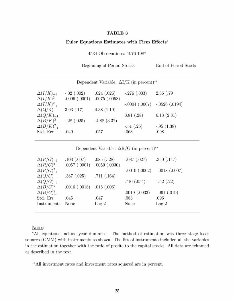
TABLE 3

Euler Equations Estimates with Firm Effects∗

4534 Observations: 1976-1987

Beginning of Period Stocks End of Period Stocks

Dependent Variable: ∆I/K (in percent)∗∗

∆(I/K)−1 -.32 (.002) .024 (.026) -.276 (.033) 2.36 (.79∆(I/K)2 .0096 (.0001) .0075 (.0058)∆(I/K)2−1 -.0004 (.0007) -.0526 (.0194)∆(Q/K) 3.93 (.17) 4.38 (1.19)∆(Q/K)−1 3.81 (.28) 6.13 (2.81)∆(B/K)2 -.28 (.025) -4.88 (3.32)∆(B/K)2−1 -.51 (.26) -.95 (1.38)Std. Err. .049 .057 .063 .098

Dependent Variable: ∆R/G (in percent)∗∗

∆(R/G)−1 .103 (.007) .085 (.-28) -.087 (.027) .350 (.147)∆(R/G)2 .0057 (.0001) .0059 (.0030)∆(R/G)2−1 -.0010 (.0002) -.0018 (.0007)∆(Q/G) .387 (.025) .711 (.164)∆(Q/G)−1 .710 (.054) 1.52 (.22)∆(B/G)2 .0016 (.0018) .015 (.006)∆(B/G)2−1 .0019 (.0033) -.061 (.019)Std. Err. .045 .047 .083 .096Instruments None Lag 2 None Lag 2

Notes:∗All equations include year dummies. The method of estimation was three stage least

squares (GMM) with instruments as shown. The list of instruments included all the variablesin the estimation together with the ratio of profits to the capital stocks. All data are trimmedas described in the text.

∗∗All investment rates and investment rates squared are in percent.

25

TABLE 4

Euler Equations Estimates with Liquidity Constrained Terms

4534 Observations: 1976-1987

Dep. Var I/K∗ R/G∗

LiquidityConstraint: No Dividends New Shares Now Dividends New Shares

(I/K)−1 .89 (.09) 1.11 (.11) (R/G)−1 1.10 (.04) 1.13 (.05)(I/K)2−1 -.0023 (.0026) -.0131 (.0038) (R/G)2−1 -.0042 (.0005) -.0054 (.0007)(Q/K)−1 .600 (1.89) .45 (.28) (Q/G)−1 .070 (.02) .072 (.032)(B/K)2−1 1.33 (.55) -1.91 (1.12) (B/G)2−1 .004 (.004) .022 (.009

Constrained at t and Unconstrained at t− 1∗∗

Dummy -1.05 (3.80) 10.5 (2.8) Dummy -5.25 (5.19) 1.69 (3.09)(I/K)−1 1.18 (.70) -.09 (.47) (R/G)−1 -1.18 (.49) -.34 (.21)(I/K)2−1 -.034 (.018) .0051 (.0126) (R/G)2−1 .022 (.009) .0038 (.0023)(Q/K)−1 -3.53 (2.36) .71 (2.07) (Q/G)−1 .038 (.458) .069 (.260(B/K)2−1 -14.3 (7.8) 7.60 (3.26) (B/G)2−1 .155 (.070) -.101 (.033)

Constrained at t and Constrained at t− 1∗∗

Dummy 8.25 (4.71) 1.15 (2.66) Dummy -2.20 (6.56) 16.2 (3.6)(I/K)−1 -1.12 (1.98) -1.01 (.32) (R/G)−1 .34 (.63) -.20 (.09)(I/K)2−1 .086 (.113) .0371 (.0108) (R/G)2−1 -.011 (.007) .0031 (.0014)(Q/K)−1 2.12 (4.22) 2.25 (.89) (Q/G)−1 .418 (1.19) .500 (.087)(B/K)2−1 -29.8 (30.9) -.34 (2.25) (B/G)2−1 -.009 (.504) -.040 (.012)F(10,4508)∗∗∗ 1.91 4.22 1.77 9.80

Notes:∗I/K and R/G are measured in percent, as before.

∗∗In columns labelled “No Dividends” the definition of liquidity constrained is D/K lessthan .00001 (dividends less than .001 percent of the capital stock). There are 77 firms whichbecome constrained and 79 which become unconstrained using this measure.In the columns labelled “New Shares” the definition of liquidity constrained is N/K greater

than .05 (new shares issues greater than 5 percent of the capital stock). There are 366 obser-vations shifting to constrained and 363 shifting to unconstrained using this measure.

∗∗∗The F-statistic is for a test that the last 10 coefficients in the regression are all zero, thatis, that there is no difference in the Euler equation estimates for firms which transit betweenconstrained and unconstrained states and the sample as a whole.

26

References

Akerlof, George A. 1970. “The Market for ’Lemons’: Quality, Uncertainty, and the Market

Mechanism.” Quarterly Journal of Economics 84: 488-500.

Arrow, Kenneth J. 1962. “Economic Welfare and the Allocation of Resources for Invention.” In

Richard Nelson, ed., The Rate and Direction of Inventive Activity. Princeton, N. J.: Princeton

University Press.

Auerbach, Alan J. 1979.“Wealth Maximization and the Cost of Capital.” Quarterly Journal of

Economics 93: 433-46.

___________. 1984. “Taxes, Firm Financial Policy, and The Cost of Capital: An Em-

pirical Analysis.” Journal of Public Economics 23: 27-57.

Auerbach, Alan J., and Mervyn A. King. 1983. “Taxation, Portfolio Choice, and Debt-Equity

Ratios: A General Equilibrium Model.” Quarterly Journal of Economics 97: 587-609.

Bernstein, Jeffrey I., and M. Ishaq Nadiri. 1982. “Financing and Investment in Plant and

Equipment and Research and Development.” In M. H. Peston and R. E. Quandt (eds.), Prices,

Competition, and Equilibrium. Oxford: Philip ALllan; Totowa, NJ: Barnes and Noble, 1986,

pp. 233-248.

Bhattacharya, Sudipto, and Jay R. Ritter. 1985. “Innovation and Communication: Signalling

with Partial Disclosure.” Review of Economic Studies L: 331-46.

27

Bond, Stephen, Richard Blundell, Costas Meghir, and Fabio Schiantarelli. 1990. ?

Bond, Stephen and Costas Meghir. 1990. “Dynamic Investment Models and the Firm’s Finan-

cial Policy.” Institute for Fiscal Studies Working Paper W90/17.

Chirinko, Robert. S. 1988a. “Will ’The’ Neoclassical Theory of Investment Please Rise?: The

General Structure of Investment Models and Their Implications for Tax Policy.” In The Impact

of Taxation on Business Investment, edited by Jack M. Mintz and Douglas D. Purvis, 109-167.

Ottawa: Economic Council of Canada.

___________. 1988b. “Distributed Lag Constraints, Asset Prices, and a New Test of the

Putty-Clay Hypothesis.” University of Chicago. Photocopied.

Chirinko, Robert S., and Steven M. Fazzari. 1990. “Market Power, Returns to Scale, and Q:

Evidence from a Panel of Firms.” University of Chicago. Photocopied.

Dammon, Robert M., and Lemma W. Senbet. 1988. “The Effect of Taxes and Depreciation on

Corporate Investment and Financial Leverage.” Journal of Finance 43: 357-74.

Fazzari, Steven M., R. Glenn Hubbard, and Bruce C. Petersen. 1988. “Financing Constraints

and Corporate Investment.” Brookings Papers on Economic Activity 1988(1): 141-205.

Gilchrist, Simon. 1990. “An Empirical Analysis of Corporate Investment and Financing Hier-

archies Using Firm Level Panel Data.” Univ. of Wisconsin-Madison. Photocopied.

Hall, Bronwyn H. 1994. “Corporate Capital Structure and Investment Horizons,” Business

28

History Review, Spring 1994.

_____________. 1992. “Investment and Research and Development at the Firm Level:

Does the Source of Financing Matter?” National Bureau of Economic Research Working Paper

No. 4096.

_____________. 1990a. “The Manufacturing Sector Master File: 1959-1987.” NBER

Technical Working Paper No. 3366.

_____________. 1990b. “The Impact of Corporate Restructuring on Industrial Re-

search and Development.” Brookings Papers on Economic Activity 1990(1): 85-136.

______________. 1990c. “The Value of Intangible Corporate Assets: An Emprical

Study of Tobin’s Q.” University of California at Berkeley and the National Bureau of Eco-

nomic Research. Photocopied.

______________. 1988a. “The Effect of Takeover Activity on Corporate Research and

Development.” In Corporate Takeovers: Causes and Consequences, edited by Alan J. Auer-

bach, 69-96. Chicago: University of Chicago Press.

______________. 1987. Time Series Processor Version 4.1 User’s Manual. Palo Alto,

CA: TSP International.

Hall, Bronwyn H., and Fumio Hayashi. 1988. “Research and Development as an Investment.”

National Bureau of Economic Research Working Paper No. 2973.

29

Hall, Robert E. 1988. “The Relation between Price and Marginal Cost in U.S. Industry.” Jour-

nal of Political Economy 96(5): 921-947.

Hayashi, Fumio. 1982. “Tobin’s Marginal q and Average q: A Neo-classical Interpretation.”

Econometrica 50: 213-24.

Hayashi, Fumio, and Tohru Inoue. 1990. “The Relation Between Firm Growth and Q with

Multiple Capital Goods: Theory and Evidence from Panel Data on Japanese Firms.” National

Bureau of Economic Research Working Paper No. 3326.

Himmelberg, Charles P., and Bruce C. Petersen. 1994. “R&D and Internal Finance: A Panel

Study of Small Firms in High-Tech Industries.” Review of Economics and Statistics __: 38-51.

Hubbard, R. Glenn, and Anil Kashyap. 1990. “Internal Net Worth and the Investment Process:

An Application to U. S. Agriculture.” Published?

King, Mervyn. 1987. “Takeover Activity in the United Kingdom.” LSE Financial Markets

Group Discussion Paper No. 0002.

King, Mervyn. 1986. “Takeovers, Taxes, and the Stock Market.” London School of Economics.

Photocopied.

Leland, Hayne E., and David H. Pyle. 1977. “Informational Asymmetries, Financial Structure,

and Financial Intermediation.” Journal of Finance 32: 371-87.

Poterba, James, and Lawrence H. Summers. 1985. “The Economic Effects of Dividend Tax-

30

ation.” In Recent Advances in Corporate Finance, edited by Edward I. Altman and Marti G.

Subrahmanyam. Homewood, Illinois: Richard D. Irwin.

Summers, Lawrence H. 1981. “Taxation and Corporate Investment: A q-Theory Approach.”

Brookings Papers on Economic Activity 1(1981): 67-127.

31