11–Applications of the Divergence Theorem:The Compressible Euler Equations

MATH 22C

1. Derivation of the Compressible Euler Equations

In this section we use the divergence theorem to derive a physical inter-pretation of the compressible Euler equations as the continuum versionof Newton’s laws of motion. Reversing the steps then provides a deriva-tion of the compressible Euler equations from physical principles. Thecompressible Euler equations are

ρt +Div(ρu = 0 (1)

(ρui)t +Div(ρuiu + pei) = 0, (2)

where ρ is the density (mass per volume), u = (ui, u2, u3) is the veloc-ity, and p is the pressure (force per area) in the fluid. For example, andfor simplicity, we can assume the pressure is a known function of thedensity through the equation of state p = p(ρ). A solution of the equa-tions would consist of functions ρ(x, t),u(x, t), x = (x, y, z) that meetsthe partial derivative constraints (1) and (2) at every point. The com-pressible Euler equations describe the motion of a compressible fluidlike air, under the assumption that there is no viscosity or dissipation.One can view these as the expressioin of Newton’s laws for a continuousmedia. That is, in words, the first Euler equation (1), (often referredto as the continuity equation), expresses conservation of mass, thatmass is nowhere created nor destroyed. The second Euler equation,

(2), is the continuum version of Newton’s force law F = ma = d(mv)dt

.It expresses that changes of momentum are due solely to gradients inthe pressure. It is interesting that when the pressure depends only onthe density, p = p(ρ), these two Euler equations stand on their own.But when the pressure depends on the temperature as well, we obtainthe full system of compressible Euler equations by including one finalequation for the energy, written most simply in the form

Et +Div[(E + p)u] = 0, (3)

where E is the energy per volume. For smooth solutions that are shockfree, the energy equation can be replaced by the much simpler entropyequation

St +Div(Su) = 0. (4)

To make sense of this, we must introduce the second law of thermo-dynamics and explain the connections between the energy density E,

1

2

the entropy density S and the pressure p. The explanation is mostinteresting because it connects up the compressible Euler equations tothermodynamics, and by this we’ll see that entropy (a measure of re-versibility) can be given a precise definition in the context of a perfectfluid, and we’ll see that (4) precisely expresses that entropy does not in-crease along particle paths when solutions are smooth. As we’ll see, thisis consistent with the fact that we neglect viscosity and heat conduc-tion in the derivation of (1)-(4). In further developments of the theoryof shock waves, (see e.g. [?]), it follows that the entropy equation (4)is violated on shock waves, but the condition that entropy increases onshock waves is sufficient to rule out the unphysical rarefaction shocksthat satisfy the Rankine-Hugoniot jump conditions.

So in this section we first use the divergence theorem to derive thephysical principles expressed by the first two Euler equations (1), (2).When p = p(ρ), this stands on its own. We next derive the continuumversion of conservation of energy expressed by the energy equation (3).We then introduce the second law of thermodynamics together withenough fluid dynamics to derive (4) and interpret it as telling us thatentropy does not increase when shocks are not present. In the finalsection we describe the fundamental polytropic equation of state thatconnects the pressure p to the energy E and entropy S for noninter-acting gas of molecules. The polytropic equation of state describes agas of identical molecules each consisting of r atoms.

The compressible Euler equations with polytropic equation of stateare a fundamental set of equations. Every term and every constantin the compressible Euler equations with polytropic equation of stateis derivable from first principles. Nothing is phenomenological (like aconstant whose value is determined by an experiment) or ad hoc (likea term added or a value assigned to make a numerical experiment fitthe data). For this reason they are fundamental to Applied Mathemat-ics, Physics and Fluid Mechanics, and they provide the main physicalsetting for the Mathematical Theory of Shock Waves. A student wholearns this has the opportunity to connect up thermodynamics, fluidmechanics, physics, and PDE’s in a unified, self-contained, fundamen-tal theory. The gain is well worth the effort!

2. The Mass and Momentum Equations

To start, restrict attention first to the first two Euler equations equa-tions (1) and (2). To derive the physical principles that underly theequations, choose any fixed volume V , integrate the equations (1), (2)

3

over V , and apply the divergence theorem. Start with (1), the so calledcontinuity equation:

0 =

∫ ∫ ∫

Vρt +Div(ρu) dV =

∫ ∫ ∫

Vρt dV +

∫ ∫ ∫

VDiv(ρu) dV.

(5)

Now in the first integral, since the integration is over x not t, we claimwe can pass the partial derivative with respect to t out through theintegral sign to get a regular derivative on the outside,

0 =

∫ ∫ ∫

Vρt dV =

d

dt

∫ ∫ ∫

Vρ dV. (6)

To verify this, use the definition of derivative directly: the definition of

d

dt

∫ ∫ ∫

Vρ dV

leads directly to

lim∆t→0

1

∆t

{∫ ∫ ∫

Vρ(x, t+ ∆t) dVx −

∫ ∫ ∫

Vρ(x, t+ ∆t) dVx

}

= lim∆t→0

∫ ∫ ∫

V

ρ(x, t+ ∆t)− ρ(x, t)

∆tdVx

=

∫ ∫ ∫

Vρt(x, t) dVx.

To the second integral in (7) we apply the Divergence theorem to ob-tain:

∫ ∫ ∫

VDiv(ρu) dV =

∫ ∫

∂Vρu · n dA. (7)

Putting these together we obtain:

4

Total MassInside V

Mass Flux

Out Through ∂V

d

dt

� � �

V

ρ dv = −� �

∂V

ρu · n dA

∆Ai

n

n

V∂V

Conservation of Mass: The time rate of change of the mass involume V equals minus the mass flux through the boundary ∂V

ρu

ρu

Conclude: The continuity equation implies that the total rate ofchange of mass inside any volume is equal to minus the flux of massout through the boundary, a precise expression of conservation of massfor that volume. Since the volume V is arbitrary, it follows that massis conserved in every volume, hence mass is conserved. But reversingthe steps, we have a derivation the continuity equation as an expressionof conservation of mass. That is, we can start by defining the physicalprinciple of conservation of momentum as meaning precisely that “the

5

time rate of change of the total mass in every volume is equal to minusthe flux of mass through the boundary” in the sense that (7) holdsfor every volume V , and from this, using the divergence theorem inreverse, we can conclude that (7) holds in every volume, and from this(using that the integral of a continuous function is zero in every volumeiff the function is identically zero) we can conclude that conservationof mass in this sense implies the continuity equation (1). We can nowtake this reversed argument as a physical derivation of (1) from a pre-cise physical expression of the principle of conservation of mass in acontinuous media. (Of course, the derivation technically is only validfor continuous functions, so shock waves are another matter!)

Consider next the second Euler equation (2),

(ρui)t +Div(ρuiu + pei) = 0,

which is really three equations, one for each i = 1, 2, 3. We now use thedivergence theorem to show that it implies conservation of momentumin every volume. That is, we show that the time rate of change ofmomentum in each volume is minus the flux through the boundaryminus the work done on the boundary by the pressure forces. This isthe physical expression of Newton’s force law for a continuous medium.For this, integrate (2) over a fixed volume V to obtain

0 =

∫ ∫ ∫

V(ρui)t dV +

∫ ∫ ∫

VDiv(ρuiu) dV +

∫ ∫ ∫

VDiv(p ei) dV.

(8)

Taking the time derivative out through the first integral and applyingthe divergence theorem to the second two integrals (as we did for thecontinuity equation) we obtain

d

dt

∫ ∫ ∫

V(ρui) = −

∫ ∫

∂V

(ρui)u · n dA−∫ ∫

∂V

p ei · n dA.

(9)

Here ρuiu is the i-momentum flux vector, with dimensions

(ρui) · u =mass× velocity

volume· distance

time=i−momentumarea time

,

so minus the first integral on the right hand side of (9) integrates overthe area to give minus the rate at which i-momentum is passing outthrough the boundary ∂V of V . Similarly, for the second integral on theright hand side of (9), the dimensions of p is force per area, ei · n = ni

equals the i’th component of the normal, so minus the second integralon the right hand side of (9) integrates over the area to give minus the

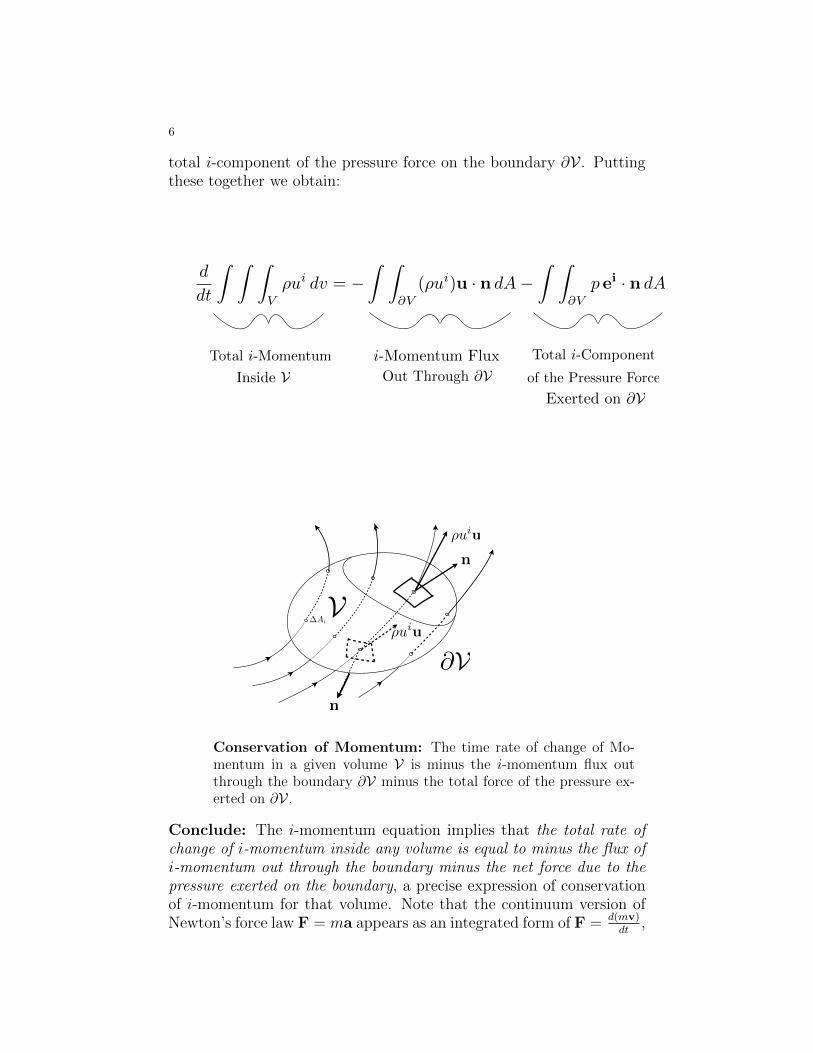
6

total i-component of the pressure force on the boundary ∂V . Puttingthese together we obtain:

Inside V Out Through ∂VTotal i-Momentum i-Momentum Flux Total i-Component

of the Pressure Force

Exerted on ∂V

d

dt

� � �

V

ρui dv = −� �

∂V

(ρui)u · n dA −� �

∂V

p ei · n dA

∆Ai

ρuiu

n

n

V∂V

ρuiu

Conservation of Momentum: The time rate of change of Mo-mentum in a given volume V is minus the i-momentum flux outthrough the boundary ∂V minus the total force of the pressure ex-erted on ∂V .

Conclude: The i-momentum equation implies that the total rate ofchange of i-momentum inside any volume is equal to minus the flux ofi-momentum out through the boundary minus the net force due to thepressure exerted on the boundary, a precise expression of conservationof i-momentum for that volume. Note that the continuum version ofNewton’s force law F = ma appears as an integrated form of F = d(mv)

dt,

7

that is, on the LHS F is replaced by the net force of the pressure onthe boundary ∂V , and the right hand side is replaced but the totaltime rate of change of i-momentum in V . Since the volume V is arbi-trary, it follows that the balance of i-momentum holds in every volume,i = 1, 2, 3, and we say that momentum is conserved. Again, we canreverse the steps, and start by defining the physical principle of con-servation of momentum as meaning precisely that “the time rate ofchange of momentum in every volume is equal to minus the flux of mo-mentum through the boundary minus the force due to the pressure onthe boundary” in the sense that (9) holds for every volume V , and fromthis, using the divergence theorem in reverse, we can conclude that (8)holds in every volume, and from this (using again that the integral ofa continuous function is zero in every volume iff the function is identi-cally zero) we can conclude that the momentum equations (2) for eachi = 1, 2, 3, follows from the principle of conservation of momentum asexpressed in (9). We can now take this reversed argument as a physicalderivation of (2) from a precise physical expression for the principle ofconservation of momentum in a continuous media. (Again, the deriva-tion technically is only valid for continuous functions, so shock wavesare another matter!)

3. The energy equation

To complete the theory of the compressible Euler equations to the casewhen p is not a function of the density alone, we consider finally theenergy equation, the fifth and last equation in the Euler system. Theequation couples to (1), (2) through the pressure when the pressuredepends on the density as well as the temperature, specific energy e orspecific entropy s, say p = p(ρ, s). The energy equation is

Et +Div((E + p)u) = 0, (10)

where

E = ρe+1

2ρ|u|2 (11)

is the total energy per volume, the sum of the internal energy per vol-ume ρe (e=e(ρ, s)=specific internal energy=the energy per mass storedin the vibrations of the molecules so that ρe is internal energy per vol-ume), and the kinetic energy 1

2ρ|u|2, the kinetic energy due to the

motion of the fluid particles. To finish we use the divergence theoremto show that (10) implies conservation of energy in every volume. Thatis, we show that the time rate of change of energy in each volume isminus the flux of energy out through the boundary minus the net rate

8

at which work is done by the pressure force acting on the boundary.This is the continuum version of Newton’s principle that the time rateof change of work should be equal to the energy change per time. Thatis, if F is a classical force, then

Work = Force×Displacement

gives

d

dtWork =

d

dtF·ds =

d

dtmdv

dtds =

(mdv

dt

ds

dt

)=

d

dt

(1

2mv2

)=

d

dtEnergy

but in the continuum case, the work per time done by the pressureforce can be stored in the internal energy of vibration as well as in thekinetic energy of motion. To see this, integrate (10) over a fixed volumeV to obtain

0 =

∫ ∫ ∫

VEt dV +

∫ ∫ ∫

VDiv(Eu) dV +

∫ ∫ ∫

VDiv(pu) dV.

(12)

Taking the time derivative out through the first integral and applyingthe divergence theorem to the second two integrals (as we did for themomentum equation) we obtain

d

dt

∫ ∫ ∫

VE = −

∫ ∫

∂V

Eu · n dA−∫ ∫

∂V

pu · n dA.

(13)

Now Eu is the Energy flux vector, with dimensions

Eu =energy

volume· distance

time=

energy

area time,

so minus the first integral on the right hand side of (9) integrates overthe area to give minus the rate at which Energy is passing out throughthe boundary ∂V of V . Consider then the second integral on the righthand side of (13). The dimensions of p are force per area (as always),so pu has dimensions

pu =force

area· distance

time=force× distancearea× time =

work

area time,

and so minus the second integral on the right hand side of (9) integratesover the area to give the total work per time done by the pressure forceacting on the boundary ∂V of V . Putting these together we obtain:

9

Inside V Out Through ∂V

d

dt

� � �

V

E dv = −� �

∂V

Eu · n dA −� �

∂V

pu · n dA

Total Energy Energy Flux Rate of Work Done

by Pressure Force

On ∂V

∆Ai

n

n

V∂V

Conservation of Energy: The time rate of change ofenergy in each volume is minus the flux of energy outthrough the boundary minus the net rate at which workis done by the pressure force acting on the boundary.

Eu

Eu

Conclude: The energy equation implies that the total rate of changeof Energy inside any volume is equal to minus the flux of Energy outthrough the boundary minus the net rate at which work is done by thepressure force on the boundary, a precise expression of conservation ofenergy for that volume. Note that the continuum version of Newton’spower law F · u = dW

dtappears with F · u replaced by pn · u where pn

is the force per area, implying pn ·u is the work per area time, so thatintegrating out the area gives the work per time. Since work is energy,

10

work per time appropriately contributes to balance the time rate ofchange of the energy expressed in the other two terms in (13). Thusthe second term on the RHS of (13) represents the pressure forcesdoing work on the fluid, and the balance of energy law (13) tells usthat the last Euler equation (10) expresses that the pressure is theonly force doing work in the fluid, thereby completing the continuumversion of Newton’s law of energy conservation. Since the volume V isarbitrary, it follows that the balance of Energy holds in every volumeas a consequence of (10), and we say that energy is conserved. Again,we can reverse the steps, and start by defining the physical principleof conservation of energy as meaning precisely that “the time rate ofchange of energy in every fixed volume is equal to minus the flux ofenergy out through the boundary minus the rate at which the pressureforce does work on the boundary” in the sense that (13) holds for everyvolume V , and from this, using the divergence theorem in reverse, wecan conclude that (10) holds in every volume. From this (using againthat the integral of a continuous function is zero in every volume iff thefunction is identically zero) we can conclude that the energy equation(2) for each i = 1, 2, 3, follows from the principle of conservation ofenergy as expressed in (13). We can now take this reversed argumentas a physical derivation of (10) from a precise physical expression for theprinciple of conservation of energy for a continuous media. (Again, thederivation technically is only valid for continuous functions, so shockwaves are another matter!)

Finally, it is interesting that although the derivation of the equationsis extremely interesting for understanding how Newton’s laws correctlyextend to a continuous medium, the derivation has helped us almostnot at all in understanding the mathematical theory of the evolutionof the compressible Euler equations that express these laws.

4. The material derivative and the entropy equation

Entropy enters the theory of the compressible Euler equations throughthe Second Law of Thermodynamics. In this section we derive theentropy equation (4) using the collection of results we already have,together with the Second Law of Thermodynamics. Entropy plays afundamental role in the theory of shock waves because shock wavesintroduce loss of information and increase of entropy, and entropy con-siderations are required to pick out the physical vs the unphysical shockwaves. The specific entropy s, the entropy per mass of the fluid, is thefifth thermodynamic variable that can be taken in place of any one ofρ, p, e and T . The starting assumption of thermodynamics is that all

11

of these five state variables can be written as a function of any two ofthem. For example, the pressure is often taken to be a function of thespecific volume v and entropy s, p = p(v, s), v = 1/ρ.

The entropy as a state variable enters through the Second Law ofThermodynamics, which for our purposes states simply that

de = Tds− pdv (14)

is an exact differential, or, solving for ds, that

ds =de

T+pdv

T(15)

is an exact differential. This (15) is exact means no more or less thanthat the right hand side comes from the gradient of a function, whichmeans there is a function s(e, v) such that

∂s

∂e= 1/T,

∂s

∂v= p/T. (16)

That is, recall from vector calculus that the line integral of a differentiallike de

T+ pdv

Tis independent of path if and only if the differential is

exact, and deT

+ pdvT

is exact just means there exists a function s(e, v)such that (16) holds. Now a class in thermodynamics would show byCarnot cycles that if de

T+ pdv

Twere not exact, then line integrals around

closed curves would not all be zero, and by this one could constructa Carnot cycle around which energy would be created from nothing.Thus, that de

T+ pdv

Tis exact is equivalent to saying there are no perpetual

motion machines. But for us, we can start by taking the second law assimply saying that ds = de

T+ pdv

Tis an exact differential, or equivalently,

solving for ds. To derive (4) from the second law, we first introducethe material derivative.

Definition 1. Let u(x, t) be a given velocity field, and let f(x, t) be anyother function of x = (x1, x2, x3) and t. Then the material derivativeof f associated with velocity u is defined to be

Df

Dt= ft(x, t) +∇xf(x, t). (17)

The material derivative represents the derivative of f along the particlepath. That is, if the curve x(t) is a particle path in the sense that itsolves the ODE

x = u(x(t), t),

thend

dtf(x(t), t) = ∇xf · x + ft =

Df

Dt.

12

The main identity used to connect up the material derivative with thecompressible Euler equations is the following (easily verified)

Div(fu) = fDiv(u) +∇f · u, (18)

which holds for any vector field u. Using these we have the followinguseful theorem:

Theorem 2. Assume ρ = ρ(x, t) and u = u(x, t) solve the the conti-nuity equation (1), and let f = f(x, t) be any smooth function. Then

(ρf)t +Div(ρfu) = ρDf

Dt. (19)

Proof: Using the product rule for partial derivatives on the first termand (18) on the second term on left of (19) gives

(ρf)t +Div(ρfu) = [ρt +Div(ρu)]f + ρ (ft +∇f · u) = ρDf

Dt, (20)

as claimed, where the first term vanishes by the continuity equation.�

Theorem 3. For smooth solutions, the continuity equation (1) is equiv-alent to either of the following two equations:

1

ρ

Dρ

Dt= −Div(u), (21)

or

1

v

Dv

Dt= Div(u). (22)

and the momentum equation (2) is equivalent to

ρDu

Dt= −∇p. (23)

Note that (22) gives meaning to the Divergence of a vector field: Namely,the divergence of a vector field gives the rate at which volumes changeper volume along the flow of the vector field. Equation (24) gives acontinuum version of Newton’s force law: Namely, “mass times accel-eration along particle paths is equal to the gradient of the pressure”,telling us that only the gradient of the pressure contributes to changesin the momentum.

Proof: For (21) use (19) to write

0 = ρt +Div(ρu) = ρt +∇ρ · u + ρDiv(u) =Dρ

Dt+ ρDiv(u)

13

which gives (21). To obtain (22) from this write

Dv

Dt=D 1

ρ

Dt= − 1

ρ2

Dρ

Dt=

1

ρDiv(u) = vDiv(u).

This is a complete proof. �

Theorem 4. Assuming the continuity equation (1), the momentumequation (2) is equivalent to

ρDu

Dt= −∇p. (24)

Proof: Write (2) in the vector form

(ρu)t +Div(ρuuT + pI) = 0,

where I is the 3× 3 identity matrix and treating u as a column vectorand its transpose uT as a row vector, uuT is the 3 × 3 rank-1 matrixwith row column entries (uiuj). Then distributing the Div gives

0 = (ρu)t +Div(ρuuT ) +Div(pI) = ρDu

Dt+∇p,

where we have applied (19) and rewritten DivpI = ∇p. This confirms(24). �

Theorem 5. Assuming the continuity equation (1) together with themomentum equation (2), the energy equation (3) is equivalent to theequation

De

Dt= −pDv

Dt= 0. (25)

Proof: Now by (11) and (18),

Et +Div(Eu) = ρDE

Dt= ρ

De

Dt+ ρu

Du

Dt, (26)

and

Div(pu) = ∇p · u + pDiv(u).

Putting these together and using (24) to cancel the ∇p · u term gives

ρDe

Dt= −pDiv(u) = −p1

v

Dv

Dt,

which readily gives (26). �

14

Theorem 6. Assuming the continuity equation (1) together with themomentum equation (2), the energy equation (3) is equivalent to theentropy equation (4), namely,

St +Div(Su) = 0, (27)

which is equivalent to

Ds

Dt= 0 (28)

Proof: Starting with the Second Law in the form (15),

Tds = de+ pdv,

it is not difficult to show that

TDs

Dt=De

Dt+ p

Dv

Dt= 0,

where we have applied the energy equation in the form (26). Thisestablishes (28). But since S = ρs is the entropy density, we can write

St +Div(Su) = (ρs)t +Div(ρsu) = ρDs

Dt= 0,

as claimed in (28). �

5. The compressible Euler Equations with PolytropicEquation of State

We end this section by summarizing the full compressible Euler equa-tions for a polytropic equation of state. The complete system of com-pressible Euler equations takes the following conservation form:

ρt +Div(ρu = 0 (29)

(ρui)t +Div(ρuiu + pei) = 0, (30)

Et +Div[(E + p)u] = 0, (31)

with

E = ρe+1

2u2, (32)

u2 ≡ |u|2 = (u1)2 + (u2)2 + (u3)2.

The system (29)-(30) is a system of five equations in the six unknownfunctions of (x, t)

u1, u2, u3, ρ, p, e,

consisting of the three components of the velocity vector u = (u1, u2, u3)(we use superscript indices to be consistent with Einstein summationconvention whereby vector components are alway up, c.f. [?]), and the

15

the remaining three variables, the density ρ, pressure p and specific in-ternal energy e are the so called thermodynamic variables. The othertwo important thermodynamic variables in shock wave theory are thetemperature T and the specific entropy s (we’ll discuss the entropy inthe next section). A principle of thermodynamics is that all of the fivethermodynamic variables can be expressed as a function of any twoof them. Since by any choice of the two independent thermodynamicvariables, there remain six unknowns and five equations, an equationof state which gives the pressure in terms of two other thermodynamicvariables, must be given to reduce the number of unknowns by one andthereby close the equations.

The most fundamental equation of state is the so called polytropic equa-tion of state given by

p = p(ρ, e) = (γ − 1)ρe, (33)

where γ is the so called adiabatic constant of the gas. Writing p =p(ρ, e) in (29)-(31) closes the compressible Euler equations into a sys-tem of five equations in the five unknowns

(u1, u2, u3, ρ, e).

To write the system in the form of a system of conservation laws

Ut + f(U)x = 0,

define the conserved quantities

U = (ρ,G,E),

usingG = (G1, G2, G3) = (ρu1, ρu2, ρu3) = ρu,

and find expressions for (p, e) in terms of U . For example, by (32),

e =E

ρ− 1

2|u|2 =

U5

U1

− 1

2

∣∣∣∣G

U1

∣∣∣∣2

,

and so

p = (γ − 1)ρe = (γ − 1)U1

(U5

U1

− 1

2

∣∣∣∣G

U1

∣∣∣∣2).

A final word on the adiabatic gas constant. The polytropic equation ofstate describes a gas of identical molecules each consisting of r atoms.In this case, assuming the ideal gas law

pv = RT, (34)

with v = 1/ρ the specific volume and R the universal gas constant,together with the assumption that the internal energy e distributes

16

equally among all the vibrational degrees of freedom, leads logically toa dervivation of (33) together with the relations, c.f. [?].

e =R

γ − 1T, (35)

γ = 1 +2

3r. (36)

In particular, for a polytropic gas (33), equation (35) tells us that theinternal energy is proportional to the temperature, with proportionalityconstant CV = R/(γ − 1) called the specific heat at constant volume,(the heat required to raise a unit mass one degree); and (36) gives theadiabatic gas constant as a function of the number of atoms r in thegas molecules. Taking the limits r = 1 and r →∞ gives the bounds

1 < γ ≤ 5

3,

the value γ = 5/3 applying to a mono-tonic gas, and γ → 1 in thelimit of very heavy molecules. In particular, air is mostly Nitrogen N2,giving a value of gamma equal to

γ = 4/3.

Conclude: Every term and constant in the compressible Euler equa-tions with polytropic equation of state is derivable from first principles.Nothing is phenomenological (like a constant whose value is determinedby an experiment) or ad hoc (like a term added or a value assigned tomake a numerical experiment fit the data). For this reason the com-pressible Euler equations with polytropic equation of state are a fun-damental set of equations for Applied Mathematics and Physics, theyanchor the subject of PDE’s by marking the starting point for FluidMechanics, and as such they provide the main physical setting for theMathematical Theory of Shock Waves.

6. Entropy of a Polytropic gas

We now show how to integrate the second law to find a formula fors as a function of v and T , and thereby show how entropy enters theformulas for a polytropic gas. By this we can find s as a function ofany other two thermodynamical variables among ρ, p, e, T .

Theorem 7. Assume (33)-(36) for a polytropic gas, and assume (14)is an exact differential, so (16) holds. Then

s = cv ln vγ−1T . (37)

17

Proof: To integrate (14), (meaning to find a function e(s, v) that meetsconditions (16)), we introduce a clever change of variables. For this,define what has come to be known as the free energy.

ψ = e− sT.For us the free energy is important simply because we can solve thesecond law when expressed in terms of ψ. For this purpose, take dif-ferentials on both sides to obtain

dψ = de− sdT − Tds.Using the second law Tds = de+ pdv, continue

dψ = de− sdT − Tds = de− sdT − de− pdv = −sdT − pdv.or

dψ = −sdT − pdv. (38)

We now solve for the value of ψ that makes (38) exact, namely, we findψ such that

∂

∂Tψ(T, v) = −s, and

∂

∂vψ(T, v) = −p. (39)

But using the idea gas law (34)

p(T, v) =RT

v,

the second equation in (39) becomes

∂

∂vψ(T, v) = −RT

v.

Remarkably, holding we can anti-differentiate this with respect to vholding T fixed to obtain

ψ(T, v) = −RT ln v + g(T ),

where g(T ) is the arbitrary function of integration. To determine g(T ),use the first equation in (39) to write

s = − ∂

∂Tψ(T, v) = − (R ln v + g′(T )) . (40)

But by the definition of ψ we also have

cvT = e = ψ(T, v) + sT = −RT ln v + g(T ) +RT ln v − Tg′(T ), (41)

the latter two terms coming from

sT = −T ∂ψ∂T

.

18

Canceling the first and third term on the RHS of (41) gives

cV T = g(T )− Tg′(T ),

which upon differentiating both sides with respect to T gives

cv = −Tg′′(T ).

By this we obtain a formula for g′′(T ), namely

g′′(T ) = −cvT,

which upon integrating once gives

g′(T ) = −cv lnT + const.

Using this in (40), and setting const. equal to zero, (only changes inentropy are measurable anyway), we obtain

s = cv ln (vγ−1T ),

as claimed. �

Finally, solving s = cv ln (vγ−1T ) for T gives

T = v1−γ exp (s

cv);

and using this in e = cvT yields the formula

e = cv1

vγ−1exp (

s

cv) ≡ e(s, v).

This together with the second law gives the equation of state of apolytropic gas in terms of (s, v):

p = −∂e∂v

(s, v) = cv(γ − 1)1

vγexp (

s

cv) ≡ p(s, v).

This is the form of the equation of state of a polytropic gas oftenquoted in the literature. In particular, replacing v = 1/ρ gives primar-ily because the speed of sound c is given by the formula

p(ρ, s) = cv(γ − 1)ργ exp (s

cv),

and it turns out the correct generalization of the speed of sound σ whenp depends on s as well as ρ is

σ =

öp

∂ρ(ρ, s).

We could obtain this by linearizing the equations just like we did forthe barotropic equation of state p = p(ρ) before.

The following important theorem gives the equation for the entropy:

19

Theorem 8. Assume the compressible Euler equations with polytropicequation of state. Then the entropy satifies the additional conservationlaw

St +Div(Su) = 0,

where

S = ρs

is the entropy per volume, or entropy density. (Note that multiplica-tion by ρ = mass/vol converts s=specific entropy=entropy/mass toS=entropy/vol.)

Proof: Write

(ρs)t +Div(ρsu) = ρts+ ρst + sDiv(ρu) + ρ∇s · u= s(ρt + div(ρu) + ρ

Conclude: The entropy is the state variable that is defined by assum-ing the second law de = Tds− pdv is an exact differential.

****************************************************

7. Derivation of the Rankine-Hugoniot Jump Conditions

In this section we apply the Divergence Theorem to derive the Rankine-Hugoniot (RH) jump conditions, which we already used to derive theshock curves of the p-system. So consider a system of conservation laws

Ut + f(U)x = 0, (42)

where U and f(U) are vectors in Rn,

U = (U1, ..., Un),

f(U) = (f1(U), ..., fn(U)).

The RH-jump conditions apply to solutions U(x, t) that are smoothon either side a curve (x(t), t) in the (x, t)-plane, but suffers a jumpdiscontinuity across the curve. So assume the shock curve (x(t), t) hasfinite speed s = x(t), and assume that U(x, t) = UL(x, t) to the leftof this curve x < x(t), and U(x, t) = UR(x, t) to the right of thiscurve x > x(t), where UL and UR are smooth functions that solve theconservation law (42). Now U cannot satisfy (42) on the shock curvebecause it suffers a jump discontinuity there, so the derivatives are notdefined. Even so, the RH condition says that the jump in a solution

20

across a shock wave must be related to the speed of the shock by thecondition

s[U ] = [f(U)]. (43)

Here, [·] around a quantity denotes the jump in that quantity from leftto right across the shock wave, so [U ] = UR − UL, [f(U)] = f(UR) −f(UL), etc. Recall that for the p-system, U = (v, u), and for fixed stateUL and constant s, the jump condition was satisfied by two curvesS1(UL) and S2(UL) that had C2 contact with the rarefaction curvesR+

1 (UL) andR+2 (UL) at UL. We then defined the wave curves Wi(UL) =

S−1 (UL) ∪ S−1 (UL), i = 1, 1, consisting the the states UR that could beconnected to UL by a shock wave of speed s = s(UL, UR) determined bythe analysis. So the question remains: where did the Rankine-Hugoniotjump conditions come from?

We now derive the RH conditions starting with the notion of a weak ordistributional solution of the conservation laws (42). In words, we showthat any solution that solves (42) on either side of a shock curve (x(t), t)will be a weak solution if and only if the RH conditions (43) hold. Tostart then we must define the notion of weak solution. For this, we lookto construct a condition that is equivalent to (42) for smooth solutions,but also applies to solutions that have jump discontinuities. The ideais to multiply the equation through by a smooth “test function” φ(x, t),integrate over any region, and integrate by parts to get the derivativesoff the unknown functions u and f(u), and onto the test function. Thecondition for a weak solution is then the condition that this integratedequation holds for all smooth test functions, and all three dimensionalregions we integrate over. Now when we integrate by parts, there will beboundary terms, and to make these vanish, we assume the test functionand all of its derivatives vanish outside the volume we integrate over.To make this precise, define:

Definition 9. The support of a function φ(x, t), denoted Suppφ, is theset of all values of (x, t) where the function φ is nonzero.

Thus outside of any set that contains the support of φ, φ ≡ 0, andso phi and all derivatives of φ vanish in the complement of that set.We use this to define a test function.

Definition 10. A test function φ(x, t) is a smooth solution such thatSuppφ is contained within a bounded set in (x, t) in −∞ < x < ∞,t > 0, that is some positive distance from t = 0.

by smooth we mean that a test function φ can be differentiated anynumber of times, and the support condition is sufficient to guarantee

21

that the function, together with all of its derivatives, vanish on theboundary of any set in −∞ < x <∞, t > 0 that contains Suppφ.

To get a condition for shock wave solutions u(x, t), multiply equation(42) by a test function φ(x, t),

utφ+ f(u)xφ = 0,

integrate over (x, t)∫ ∞

0

∫ ∞

−∞utφ+ f(u)xφ dxdt =

∫ ∫

Kutφ+ f(u)xφ dxdt, (44)

where we used the fact that φ(x, t) vanishes for (x, t) on the boundaryof K, because K contains the suppport of φ. Denoting the boundary ofK by ∂K and assuming without loss of generality that K is containedwithin −∞ < x <∞, t > 0, we can integrate (45) by parts to obtain∫ ∫

K(utφ+ f(u)xφ) dxdt =

∫ ∫

K(uφ)t + (fφ)xφ dxdt

−∫ ∫

Kuφt + f(u)φx dxdt.

where we have applied the Leibniz product rule to write the integralas a divergence, plus the integration by parts term. By the divergencetheorem, the first term reduces to an integral on the boundary ∂Kwhere φ and all its derivatives vanish, so this term is zero, i.e.,

∫ ∫

K(utφ+ f(u)xφ) dxdt =

∫ ∫

KDivx,t (fφ, uφ) dxdt

−∫

∂K(fφ, uφ) · n dxdt = 0.

Thus we conclude that for any test function φ and solution u of (42)we have∫ ∞

0

∫ ∞

−∞utφ+ f(u)xφ dxdt = −

∫ ∞

0

∫ ∞

−∞uφt + f(u)φx dxdt, (45)

so long as u is smooth enough so that the derivatives ut and f(u)x exist.For shock wave solutions, the right hand side of (45) makes sense, butthe left hand side of (45) does not.

Definition 11. We call u(x, t) a weak or distributional solution of theconservation law (42) if∫ ∞

0

∫ ∞

−∞uφt + f(u)φx dxdt = 0 (46)

for all smooth test function φ(x, t).

22

The purpose of the section is to to use the Divergence Theorem toprove the following theorem which, in words, states that a shock wavesolution is a weak solution of (42) if and only if the RH-jump conditionshold across the shock.

Theorem 12. Assume u(x, t) is a smooth solution of (42) on eitherside of a smooth shock curve (x(t), t), but discontinuous across it. Thenu is a weak solution if and only if s[u] = [f ] holds at each point of theshock. That is, if and only if

x(uR − uL) = (f(uR)− f(uL)).

Proof: Assume the φ is a smooth test function with support K, andassume the values uL(x, t) of u on the left and uR(x, t) on the right ofthe shock curve (x(t), t), both solve (42). Let K = KL∪KR decomposeK into the part left and right of the shock curve (x(t), t), respectively,(c.f. Figure 1.) Thus we can write the weak condition as∫ ∞

0

∫ ∞

−∞uφt + f(u)φx dxdt =

∫ ∫

Kuφt + f(u)φx dxdt

=

∫ ∫

KL

uLφt + f(uL)φx dxdt+

∫ ∫

KR

uRφt + f(uR)φx dxdt, (47)

where uL and uR are smooth in K. Thus we can apply the divergencetheorem in the derivation of the weak conditions in reverse to get thederivative back onto u and f(u), and then apply (42). But the bound-ary condition at the shock, where φ need not vanish, will produce theRH condition. Starting on the left, we get∫ ∫

KL

uLφt + f(uL)φx dxdt =

∫ ∫

KL

(uLφ)t + (f(uL)φ)x dxdt

−∫ ∫

KL

(uL)tφ+ f(uL)xφ dxdt.

But by the divergence theorem,

∫ ∫

KL

(uLφ)t + (f(uL)φ)x dxdt =

∫

Γ

−−−−−→(fL, uL) · nL φ ds, (48)

and ∫ ∫

KL

utφ+ f(u)xφ dxdt = 0,

because u solves (42) in KL, so we obtain∫ ∫

KL

uLφt + f(uL)φx dxdt =

∫

Γ

−−−−−→(fL, uL) · nLφ ds,

23

where Γ dentoes the shock curve (x(t), t). Note that ut + f(u)x makessense and vanishes in KL and KR separately because we don’t have totake derivatives at the shock itself. (We can take the derivatives allthe way up to the shock curve by continuity of u and its derivatives oneither side of the shock.) Note that the boundary of KL where φ neednot vanish is exactly the shock curve (x(t), t), which we have denotedby Γ, and nL denotes the outer normal to KL.Similarly on the right side K of the shock curve we obtain∫ ∫

Γ

uRφt + f(uR)φx dxdt =

∫

Γ

−−−−−→(fR, uR) · nR φ ds.

Putting (49) and (49) together we obtain∫

Γ

−−−−−→(fL, uL) · nLφ ds+

∫

Γ

−−−−−→(fR, uR) · nR φ ds

=

∫

Γ

−−−−−−−−−−−−−→(fR − fL, uR − uL) · nR φ ds = 0, (49)

where we used that nL = −nR. But on the shock curve (x(t), t) thenormal vector nR = −i + xj. That is, the parametrization of the shockcurve Γ with respect to t is

r(t) = x(t)i + tj,

sov′(t) = xi + j,

and the unit tangent vector T = |v|/|v| is

T =xi + j√x2 + 1

.

Hence the outer normal nR to γ is

nR =−i + xj√x2 + 1

.

Using this in (50) gives the result∫

Γ

{s[u] + [f ]}φ ds = 0,

The result, then, is that a weak solution u(x, t) of the conservation law(42) that is a smooth solution on either side of a shock curve, mustsatisfy (50) for every smooth test function φ. It follows that we musthave s[u] + [f ] = 0 at each point of the shock, for if it were nonzero atsome point on the shock curve, then we could cook up a test functionwith support near that point such that (50) was nonzero. Conversely,if s[u] + [f ] = 0 all along the shock curve, and u is a strong solution on

24

either side, then (50) is zero, and hence working backwards we wouldfind that u is a weak solution as well. This completes the proof thetheorem, and the derivation of the Rankine-Hugoniot jump conditions.