1 variational models for the incompressible euler equations
TRANSCRIPT
1
Variational models for the incompressibleEuler equationsSara Daneri, Alessio Figalli
1.1 Introduction
In these notes we consider different models to describe the motion of homo-geneous incompressible fluids inside a bounded Lipschitz domain D ⊆ Rdwithout the action of external forces.
A classical model is given by the Euler equations, which describe the evo-lution of the velocity field of the fluid v : [0, T ]×D → Rd,
∂tv +(v · ∇
)v +∇p = 0 in [0, T ]×D
div v = 0 in [0, T ]×D,(1.1)
coupled with the boundary condition
v · ν = 0 on [0, T ]× ∂D, (1.2)
where ν is the unit exterior normal to ∂D. If v = (v1, . . . , vd) : [0, T ] ×D →Rd, then (adopting the summation convention) div v = ∂jv
j is the spatialdivergence of v, ∇v is the spatial gradient, and
(v · ∇
)v is the vector in Rd
whose i-th component is given by vj∂jvi. Hence, (1.1) is a system of (d + 1)
equations for the (d + 1) unknowns (v1, . . . , vd, p), where p : [0, T ] ×D → Rphysically represents the pressure field.
The motion of an incompressible fluid inside D can be described alsofrom a Lagrangian viewpoint, namely through the motion of its particleswith respect to their initial position. To pass from the Eulerian to the La-grangian formulation, let us assume that v is a smooth solution of (1.1), andlet g : [0, T ]×D → Rd be the flow map
g(t, a) = v(t, g(t, a)) (t, a) ∈ [0, T ]×Dg(0, a) = a a ∈ D.
(1.3)
Due to the boundary condition (1.2), we get g(t,D) = D for all t ∈ [0, T ].Moreover, differentiating (1.3) and using the classical identity
2 1 Variational models for the incompressible Euler equations
d
dε |ε=0
det(A+ εBA) = tr(B) det(A),
one obtains∂t(det∇g(t, a)
)= div v(t, g(t, a))det∇g(t, a), (1.4)
which because of the incompressibility constraint div v = 0 implies
det∇g(t, a) ≡ 1, ∀ t ∈ [0, T ].
Hence g(t) := g(t, ·) belongs to the space SDiff(D) of orientation andmeasure-preserving diffeomorphisms of D. Moreover, differentiating (1.3) withrespect to t and using the Euler equations (1.1), we obtain that the mapt 7→ g(t) satisfies the ODE
g(t, a) = −∇p(t, g(t, a)) in [0, T ]×D (1.5)
with the constraint
g(t) ∈ SDiff(D), ∀ t ∈ [0, T ]. (1.6)
On the other hand it is not difficult to show that the converse is also true:in the smooth case v : [0, T ]×D → Rd solves the Euler equations (1.1)-(1.2)with initial condition v(0) = v0 if and only if its flow map g satisfies theODE (1.5)-(1.6) with the initial conditions g(0) = v0 and g(0) = iD, beingiD : D → D the identity map.
In the first part of these notes (Section 1.2) we review some results con-cerning the existence and uniqueness of solutions of (1.1), both in the classicaland in the weak (distributional) setting. In Section 1.2.1 we will focus on theproof of the global (in time) existence and uniqueness of weak solutions withbounded vorticity in dimension d = 2 ([Yud63]). If on the one hand localexistence and uniqueness of classical solutions of (1.1) can be obtained undersuitable smoothness assumptions on the initial data (see e.g. [BM02]), on theother hand no global existence result is available in dimension d ≥ 3, noteven of weak (distributional) solutions. In Section 1.2.2 we present the notionof generalized measure-valued solutions introduced by DiPerna and Majda in[DiPM87]. The measure-valued solutions of DiPerna and Majda are globallydefined and include the vanishing viscosity limits of Leray solutions of Navier-Stokes equations. Despite the fact that they are not unique, a weak-stronguniqueness result holds ([BDS11]).
The second and more substantial part of these notes (Sections 1.3, 1.4 and1.5) is devoted to the study of some variational formulations of the problem(1.5).
The starting point of these variational models is Arnold’s interpretationof the ODE (1.5) as the geodesic equation on SDiff(D), seen (formally) asan infinite-dimensional submanifold of L2(D;Rd) with respect to the inducedmetric ([Arn66]). Therefore, in analogy with the finite dimensional Rieman-nian setting, one is led to study the following:
1.1 Introduction 3
Problem 1.1. Given g0, gT ∈ SDiff(D), find a smooth curve [0, T ] 3 t 7→g(t) ∈ SDiff(D) minimizing the energy
E(g) = T
∫ T
0
1
2‖g(t)‖2L2(D;Rd) dt, (1.7)
among all curves in [0, T ] 3 t 7→ g(t) ∈ SDiff(D) satisfying g(0) = g0,g(T ) = gT .
Notice that Problem 1.1 is essentially different from (1.5). Indeed, insteadof prescribing the initial velocity of the curves g(0) = v0, we assign theirfinal position g(T ). Moreover, we look only for minimizers of (1.7) instead ofconsidering all its critical points, which again formally correspond to solutionsof (1.5).
As we will see in Section 1.3.1, the existence of energy minimizing curvesfor (1.7) is guaranteed only if g0 and gT are close in a very strong topology([EM70]). In general, as shown by Shnirelman ([Shn87], [Shn94]) there couldbe no curves of finite energy if d = 2, or the infimum in (1.7) could not beattained.
From the classical variational viewpoint, the main difficulties lie in the factthat the topology induced by the energy (1.7) does not permit to preserve theconstraint of being diffeomorphisms, or even maps, for all t ∈ [0, T ].
Even trying to attack the minimization problem (1.7) with the simplerstrategy of projecting on SDiff(D) time-discretized geodesics in L2(D;Rd)(see Section 1.3.2), the need for relaxation in space is evident.
These preliminary considerations led Brenier [Bre89] to introduce a weakervariational formulation of (1.7), allowing both for non-injective flow mapst 7→ g(t) taking values in the space of (Lebesgue) measure-preserving maps,and also for the splitting/crossing of fluid particles (see Section 1.4).
Assuming g0 to be equal to iD (as explained in Section 1.3.1, this can bedone without loss of generality), the dynamics of the possible trajectories fol-lowed by the particles is now described by probability measures concentratedon the space of continuous paths Ω(D) := C([0, T ];D).
More precisely, one considers the following minimization problem (here etdenotes the evaluation map at time t, that is et(ω) = ω(t), and LD denotesthe Lebesgue measure on D renormalized in such a way that LD(D) = 1, seeSections 1.3 and 1.4 for more details):
Problem 1.2. Given h ∈ SDiff(D), find a minimizer of the action
A(η) = T
∫Ω(D)
∫ T
0
1
2|ω(t)|2 dt dη(ω) (1.8)
among all η ∈ P(Ω(D)) satisfying
(et)]η = LD, ∀ t ∈ [0, T ], (1.9)
and(e0 × eT )]η = (iD × h)]LD.
4 1 Variational models for the incompressible Euler equations
Following Brenier [Bre89], probability measures η ∈ P(Ω(D)) such that (1.9)holds are called generalized incompressible flows.
Notice that any flow of measure-preserving diffeomorphisms t 7→ g(t) ∈SDiff(D) with g(0) = iD induces a generalized incompressible flow ηg :=(Φg)]LD, where Φg : D → Ω(D), Φg(a) = g(·, a), and E(g) = A(ηg).
However, the converse is not always true: by definition, for any interme-diate time t ∈ (0, T ), (e0, et)]η ∈ Γ (D) –where Γ (D) = γ ∈ P(D × D) :(π1)]γ = LD, (π2)]γ = LD is the set of measure-preserving transport plansof D– but (e0, et)]η is deterministic only if there exists a (measure-preserving)map ht : D → D such that (e0, et)]η = (iD×ht)]LD. However, there are gen-eralized incompressible flows connecting the identity to some h ∈ SDiff(D)for which (e0, et)]η is not deterministic at some intermediate time (see Sec-tion 1.4.4). Hence, in Section 1.4.1 we will describe an extension of Brenier’sformulation, introduced by Ambrosio and Figalli in [AF09], which allows toconnect any η, γ ∈ Γ (D) and then to study the behaviour of generalized flowsalso for intermediate times.
In Section 1.4.2 we prove the existence of minimizers of Problem 1.2 con-necting iD to any η ∈ Γ (D) when D is the d-dimensional torus D = Td, d ≥ 2([Bre89]). This result can be extended also to other Lipschitz domains D andflows between any η, γ ∈ Γ (D) ([Shn94],[AF09]).
In Section 1.4.3 we deal with the consistency of minimizers of the action(1.8) with classical solutions of (1.5). As proved by Brenier in [Bre89], underappropriate assumptions on the pressure vector field (second spatial deriva-tives uniformly bounded in time) and for T sufficiently small, the generalizedflows are unique and induced by classical solutions. However, for times largerthan a fixed T (depending on the L∞-norm of the second spatial derivativesof p) the uniqueness property may be lost, even among classical solutions. Aninteresting non-uniqueness example on the 2-dimensional disc is presented inSection 1.4.4 (see [Bre89], [BFS08]).
However, despite the lack of uniqueness of action minimizing flows, in[Bre99] (see Section 1.5.1) it has been shown that, given h ∈ S(D) for whichthe infimum of the action among generalized incompressible flows betweeniD and h is finite, there exists a distribution p which acts as a Lagrangemultiplier for the incompressibility constraint. More precisely, a generalizedincompressible flow is a minimizer of the action between iD and h if and onlyif it minimizes an augmented action functional (including a distribution p)among a broader class of flows, called almost-incompressible generalized flows(see Section 1.5.1).
A surprising feature of this variational model is that this distribution pis unique, up to trivial modifications (see Section 1.5.2), and is called thepressure field since it coincides with the usual one in the smooth case.
In Section 1.5.3 we present an equivalent formulation of the minimiza-tion Problem 1.2 of mixed Eulerian-Lagrangian type. This model, introducedby Brenier in [Bre99], provides a finer description of the trajectories fol-lowed by the optimal generalized flows, and allows to show that p is indeed

1.2 Incompressible Euler equations 5
a function, and not merely a distribution ([Bre99], [AF08]). In particular,
p ∈ L2loc((0, T );L
d/(d−1)loc (D)).
In Section 1.6 we restrict for simplicity to the d-dimensional torus Tdand we report the analysis made in [AF09] on the necessary and sufficientconditions for optimality of generalized flows. In particular, as in the smoothcase, we will see (Theorem 1.54) that almost every trajectory followed by anoptimal flow is a local minimizer of the action∫ T
0
1
2|ω(t)|2 − p(t, ω(t)) dt
among all curves of finite action connecting ω(0) and ω(T ). The main difficultyhere is to define the value of p along curves in D and near t = 0 and t = T ,due to the local integrability assumption. A second necessary condition willbe related to the local optimal transportation properties of the intermediateplans determined by the optimal generalized flows (see Theorem 1.56). In theend, we will see that the validity of both these necessary conditions is alsosufficient for optimality (Theorem 1.57).
1.2 Incompressible Euler equations
In this section we consider the Cauchy problem for the Euler equations (1.1)with boundary condition (1.2). Here D is a bounded and simply connecteddomain of Rd with C2 boundary, and we denote by v0 : D → Rd the initialcondition.
The existence of classical (i.e., sufficiently smooth) solutions was alreadyinvestigated by Gunther and Lichtenstein at the end of the ’20s. In [Gun27]and [Lic25] they proved local (in time) existence and uniqueness of velocityfields v ∈ C1,λ, 0 < λ < 1, as soon as v0 is sufficiently smooth. As for classicalsolutions, an existence result stated in modern form is the following (see e.g.[Tay96], Chapter 17, Theorem 2.1 and Proposition 2.2, or [BM02], Theorem3.4):
Theorem 1.3. If v0 ∈ Hs for some s >[n2
]+ 1, then ∃T = T (‖v0‖Hs) > 0
such that there exists a unique classical solution of (1.1) on [0, T ]×D.
However, no global existence theorem valid in all dimensions is presentlyknown.
A property satisfied by classical solutions is energy conservation. Indeed,
d
dt
∫D
1
2|v(t, x)|2 dx =
∫D
vi∂tvi (1.1)
= −∫D
vivj∂jvi −∫D
vi∂ip
= −∫D
vj∂j|v|2
2+
∫D
∂ivip
=
∫D
∂jvj
(|v|2
2+ p
)(div v=0)
= 0.
6 1 Variational models for the incompressible Euler equations
Henceforth, the natural energy space where to look for weak distributionalsolutions is L∞([0, T ];L2(D;Rd)). As observed in [DLS09], the search for weakdistributional solutions of the Euler equations, other than being natural fromthe PDEs viewpoint, comes also from Kolmogorov’s theory of turbulence.
Definition 1.4 (Distributional solutions). We say that a vector field v ∈L∞([0, T ];L2(D;Rd)) is a weak solution to the Cauchy problem for (1.1) withinitial datum v0 ∈ L2(D;Rd) if, for all ϕ ∈ C∞c ([0, T )×D;Rd) with divϕ = 0and for all ξ ∈ C∞(D),∫ T
0
∫D
v · ∂tϕ+ (v ⊗ v) : ∇ϕdx dt+
∫D
v0ϕdx = 0 (1.10)
and ∫D
v(t, ·) · ∇ξ = 0, for L1-a.e. t ∈ [0, T ].
We recall that any weak distributional solution v ∈ L∞([0, T ];L2(D;Rd)) of(1.1) belongs (up to redefining it on a L1-negligible set of times) to the spaceC([0, T ];L2
w(D;Rd)) (see e.g. [DLS10], Lemma 7.1).Let us mention that, with the exception of the case d = 2 in which the
existence and uniqueness of global weak solutions can be proved under addi-tional regularity assumptions on the vorticity of the initial data (see Section1.2.1), in higher dimensions no general theorem providing global solutions isknown.
Moreover, as shown first by Scheffer in [Sch93] and Shnirelman [Shn97],weak solutions may not be unique. In [DLS09], De Lellis and Szekelyhidi in-troduced a new framework in which to study oscillatory non-uniqueness phe-nomena for the Euler equations and proved the following theorem (implyingthe results of [Sch93] and [Shn97] with a much simpler proof).
Theorem 1.5. For all d ≥ 2, there exist v ∈ L∞(R×Rd;Rd) and p ∈ L∞(R×Rd), solving (1.1) in the distributional sense, such that v is not identically zeroand supp v, supp p are compact subsets of R× Rd.
We note that the fact that Theorem 1.5 holds also in dimension two doesnot clash with the uniqueness result of Section 1.2.1 (see Theorem 1.6), sinceDe Lellis and Szekelyhidi’s solutions do not satisfy the required regularityassumptions. Theorem 1.5 shows that there are very pathological examples ofsolutions to Euler: since the support of v is compact in space-time, it meansthat at some initial time the fluid is at rest (v ≡ 0) but then at some moment,without the action of any external force, it starts suddenly to move, and finallyit comes back to rest. In particular, for such solutions the conservation of theL2 norm is violated.
1.2 Incompressible Euler equations 7
1.2.1 Weak solutions in the two dimensional case
In two dimensions much more is known about the existence of global solutionsof (1.1). Indeed, as we will see, in the two dimensional case the equationsatisfied by the vorticity of v has a nice structure, and the results obtained forthis equation translate, under suitable regularity assumptions on the initialdata, into the global (in time) existence and uniqueness of weak solutions ofthe Euler equations.
Recall that, for any w ∈ L1(D;R2), the vorticity of w is the distributiondefined by
curlw := ∂2w1 − ∂1w
2.
Moreover, for time dependent vector fields u ∈ L1([0, T ]×D;R2) we will usethe same notation curlu to denote the time-dependent distribution
t 7→ curlu(t) := curl (u(t, ·)). (1.11)
The global existence of classical solutions for sufficiently smooth initialdata was proved by Wolibner [Wol33]; Kato presented the result in a modernform in [Kat68].
The generalized solutions in the two dimensional case were first introducedby Yudovich in [Yud63], providing the following global existence and unique-ness theorem for initial data having bounded vorticity.
Theorem 1.6 ([Yud63]). For any v0 ∈ L2(D;R2) such that curl v0 ∈L∞(D), there exists a unique weak distributional solution of (1.1) v ∈L∞([0,+∞);L2(D)) with initial condition v0 and satisfying
curl v ∈ L∞([0,+∞)×D)
More precisely, Yudovich proved that the global existence of solutionsholds whenever curl v0 ∈ Lp(D) for any given p > 1. However, the unique-ness property was shown only in the case of bounded vorticity. In [Yud95],the uniqueness result was improved allowing for initial vorticities which be-long to ∩p∈[1,+∞)L
p, with some restriction on the growth of the Lp-norms asp→ +∞. The existence part of Theorem 1.6 was improved by Delort [Del91]to initial vorticities of the form ω0 = ω′0 + ω′′0 , where ω′0 is a non-negativecompactly supported Radon measure in H−1(R2) and ω′′0 an Lp compactlysupported function (p > 1). Delort’s solutions belong as well to the spaceL∞loc([0,+∞);L2
loc(D)) and their vorticities ω(t) are, for all t ∈ [0,+∞), of theform ω = ω′+ω′′, where ω′ is a positive measure with mass uniformly boundedin t by the mass of ω′0 and ω′′ ∈ L∞([0,+∞);Lq(D)), for all q ∈ [1, p]. Thetechnique used in [Del91] is however rather different w.r.t. the one used byYudovich to prove Theorem 1.6, and we will not describe it here.
The aim of this Section is to give a proof of Theorem 1.6. As anticipated,the first idea to obtain weak solutions of (1.1) is to study the PDE satisfiedby their vorticity (Propositions 1.9 and 1.10).

8 1 Variational models for the incompressible Euler equations
In Proposition 1.8 we will see that it is possible to reconstruct a vector fieldfrom its vorticity, under suitable integrability assumptions. Before giving theprecise statement, we need to define some elliptic and distributional operators.
For any ρ ∈ L∞(D), we denote by 4−1ρ the weak solution of the Dirichletproblem
4ψ = ρ in D
ψ = 0 on ∂D(1.12)
By standard elliptic theory, ψ = 4−1ρ ∈ W 2,p(D) ∩ W 1,p0 (D) for all p ∈
[2,+∞). Moreover, one has the bounds
‖4−1ρ‖W 2,p(D) ≤ C(p,D)‖ρ‖L∞(D), p ∈ [2,+∞). (1.13)
Denoting by ∇⊥ the distributional operator
∇⊥φ := (∂2φ, −∂1φ), (1.14)
for any ρ ∈ L∞ defineK(ρ) := ∇⊥4−1ρ, (1.15)
where ∇⊥4−1 is the composition of (1.12) and (1.14).Notice that, by (1.13) and (1.14), K(ρ) ∈W 1,p(D;R2) for all p ∈ [2,+∞).
Moreover, one has the following quantitative estimate on the growth withrespect to p of its W 1,p norms, which will be used in the proof of Theorem1.6 (see e.g. [Ste70]):
Lemma 1.7. For any ρ ∈ L∞(D),
‖∇K(ρ)‖Lp(D;R2) ≤ C(D)p2
p− 1‖ρ‖L∞(D), (1.16)
where C(D) is a geometric constant.
Proposition 1.8. Let ρ ∈ L∞(D). Then
curlK(ρ) = ρ, (1.17)
and K(ρ) is the unique function satisfying (1.17) and lying in the space
H :=
u ∈ L2(D;R2) : div u = 0, u · ν = 0 on ∂D
.
Proof (Proposition 1.8). Set ψ := 4−1ρ. Then K(ρ) = ∇⊥ψ = (∂2ψ,−∂1ψ)and curlK(ρ) = 4ψ = ρ. Moreover, since div∇⊥ = 0, divK(ρ) = 0. Finally,since K(ρ) = ∇⊥ψ and ψ = 0 on ∂D, it follows that K(ρ) · ν = ∂ψ
∂τ = 0 on∂D. Hence K(ρ) ∈ H.
1.2 Incompressible Euler equations 9
In order to prove that K(ρ) is unique in H, let us assume that ∃w ∈ Hsuch that curlw = ρ and prove that u := K(ρ)− w is identically zero.
Since both K(ρ) and w have the same curl and are divergence free, u ∈ Hand curlu = 0. Then, since by assumption D is simply connected, there existsφ : D → R satisfying
∇φ = u in D,∂φ∂ν = 0 on ∂D,
which implies (since div u = 0)4φ = 0 in D,∂φ∂ν = 0 on ∂D.
Hence φ is constant, and so u = 0 as required.
From now on, as done in (1.11) for the vorticity of time dependent vec-tor fields, for any function ω ∈ L2([0, T ] × D) we define K(ω) as the timedependent distribution
K(ω) : t 7→ K(ω(t, ·)).
Proposition 1.9. Any smooth vector field v : [0, T ]×D → R2 is a solution of(1.1) satisfying the boundary condition (1.2) if and only if the smooth scalarfield ω : [0, T ] ×D → R defined as ω(t, ·) := curl v(t, ·) satisfies the transportequation
∂tω + (K(ω) · ∇)ω = 0. (1.18)
Proof (Proposition 1.9). Let v : [0, T ]×D → R2 be a smooth solution of (1.1).Then, by simple computations, it is possible to show that the smooth scalarfield ω satisfies (1.18).
Indeed, taking the curl in (1.1) one obtains
∂tω + (v · ∇)ω + div vω = 0,
that coincides with (1.18) since v is divergence free. (This is a peculiarity ofthe two dimensional case, since in higher dimensions the right-hand side ofthis equation contains an additional term.)
Viceversa, if a smooth scalar field ω satisfies
∂tω + (K(ω) · ∇)ω = 0 in (0, T )×D, (1.19)
then the vector field v(t, ·) := K(ω(t, ·)) is a solution of the Euler equations.Indeed, the vorticity of the vector field w = (w1, w2) whose components
are given bywi = ∂tv
i + vj∂jvi
coincides with the left-hand side of (1.19). Hence it is identically 0, and sinceD is simply connected there exists a scalar field p : [0, T ] × D → R whosespatial gradient satisfies (1.1).

10 1 Variational models for the incompressible Euler equations
In the distributional setting, an analogous correspondence between weaksolutions of (1.18) and weak solutions of the Euler equations having boundedvorticity holds.
Proposition 1.10. Let v0 ∈ L2(D;R2) with curl v0 ∈ L∞(D). Then, v ∈L∞([0, T ];L2(D;R2)) is a weak solution of (1.1) with initial datum v0 ∈L2(D) and curl v ∈ L∞([0, T ]×D) if and only if ω := curl v ∈ L∞([0, T ]×D)is a weak solution of (1.18) with initial datum ω0 := curl v0, namely∫ T
0
∫D
ω∂tφ+ ωK(ω) · ∇φdx dt+
∫D
ω0φ(0) dx = 0, (1.20)
for all φ ∈ C∞c ([0, T )×D).
The proof follows by standard integration by parts arguments.Thanks to Proposition 1.10, Theorem 1.6 is an immediate consequence of
the following result.
Theorem 1.11. For any ω0 ∈ L∞(D), there exists a unique weak solutionω ∈ L∞([0,+∞)×D) of the Cauchy problem (1.18) with initial datum ω0.
Proof (Theorem 1.11).ExistenceThe existence of a solution can be obtained via an explicit Euler scheme
combined with a regularization argument. Let ρεε>0 ⊂ C∞c (D) be a familyof smooth mollifiers with supp(ρε) ⊂ Bε, and consider the following scheme:for any n ∈ N we define ωεn as the solution of the linear transport equation
∂tωεn +K(ωεn) · ∇ωεn = 0, in (0,+∞)×Dε,
ωεn(0) = ω0 ∗ ρε,(1.21)
where we have extended ω0 to be identically zero outside D, and
ωεn(t) := ωεn(k/n) if t ∈ [k/n, (k + 1)/n), k ∈ N.
More precisely, once ωεn has been constructed up to a time k/n, we use ωεn(k/n)to define the vector field K(ωεn) on the time interval [k/n, (k + 1)/n], andthen we can define ωεn on the interval [k/n, (k+ 1)/n] by using the method ofcharacteristics: ωεn is given by the representation formula
ωεn(t, x) = ωεn(k/n, (Xε
n,k)−1(t− k/n, x)), t ∈ [k/n, (k + 1)/n], (1.22)
where Xεn,k(s, x) = K(ωεn(k/n))
(Xεn,k(s, x)
),
Xεn,k(0, x) = x,
is the flow of K(ωεn(k/n)) in D (recall that by definition K · ν = 0 on ∂D, sothe flow preserves D).
1.2 Incompressible Euler equations 11
In particular, by induction on k, one immediately checks that ωεn is smoothfor every n. Moreover, by (1.22),
‖ωεn‖L∞([0,+∞)×Dε) ≤ ‖ω0 ∗ ρε‖L∞(Dε) ≤ ‖ω0‖L∞(D) (1.23)
and, by elliptic regularity (see (1.13))
‖K(ωεn)‖L∞([0,+∞);W 1,p(Dε)) ≤ C(p,D)‖ωεn‖L∞([0,+∞)×Dε)
≤ C(p,D)‖ω0‖L∞(D)
(1.24)
for all p ∈ [1,+∞) and for some geometric constant C(p,D) depending onlyon p and on the domain D.
Let us consider sequences εjj∈N, njj∈N such that εj → 0 and nj →∞as j →∞. Up to subsequences, (1.23) guarantees that ∃ω ∈ L∞([0,+∞)×D)
such that ωεjnj∗ ω in L∞([0,+∞)×D). In particular, by linearity of K, it is
immediate to check that K(ωεjnj )
∗ K(ω) in L∞([0,+∞)×D). We now want
to show that actually the convergence of K(ωεjnj ) is strong, and that it is still
valid if instead of K(ωεjnj ) we consider K(ω
εjnj ).
To this aim we observe that, since div (K(ωεn)) = 0, (1.21) can be rewrittenas
∂tωεn = −div (K(ωεn)ωεn) , (1.25)
and the linearity of K implies that
∂tK(ωεn) = −∇⊥4−1 [div (K(ωεn)ωεn)] . (1.26)
Hence, thanks to (1.24), the maps t 7→ ∂tK(ωεjnj (t, ·)) are uniformly bounded
in Lp(D;R2), uniformly in time. So, using (1.24) again, we can apply Aubin-Lions’ lemma to deduce that K(ω
εjnj )→ K(ω) strongly in L1
loc([0,+∞)×D).Finally, we use (1.25), (1.23), and (1.24) to estimate K(ωεn)−K(ωεn):
‖K(ωεn)−K(ωεn)‖L∞([0,+∞),L2(D)) ≤ ‖ωεn − ωεn‖L∞([0,+∞),H−1(D))
≤ supk∈N
∫ (k+1)/n
k/n
‖∂tωεn(t)‖H−1(D) dt
≤ supk∈N
∫ (k+1)/n
k/n
‖K(ωεn(t))ωεn(t)‖L2(D) dt
≤ C
n,
which implies that also K(ωεjnj )→ K(ω) in L1
loc([0,+∞)×D).Thanks to these facts, by taking the limit in (1.21) we obtain that ω is a
solution of (1.18) with initial datum ω0.
UniquenessLet ω, δ be two weak solutions of (1.18) with initial condition ω0 ∈ L∞(D),
and let v = K(ω), w = K(δ) be the corresponding weak solutions of the
12 1 Variational models for the incompressible Euler equations
Euler equations (see Proposition 1.10). Then, it is sufficient to show thatu := v − w = 0.
By (1.13), (1.26), and the boundedness of ω, one has that, for all p ∈[1,+∞),
v ∈ L∞([0,+∞);W 1,p(D;R2)), ∂tv ∈ L∞([0,+∞);Lp(D;R2)), (1.27)
which implies in particular v ∈ C([0,+∞);Lp(D;R2)) for all p ∈ [1,+∞).Since the same bounds hold also for w, by a simple computation using (1.10)for both v and w (observe that, thanks to the above bounds, v and w are alsoadmissible test functions) we get (recall that u(0) = 0)∫
D
|u|2(t, x) dx = −∫ t
0
∫D
(∂vi
∂xk+∂vk
∂xi
)uiuk dx ds. (1.28)
Let us now define the following functions:
f :=|u|2
2, aik :=
∂vi∂xk
+∂vk∂xi
, g :=
√∑i,k
a2ik, L(t) :=
∫D
f(t, x) dx.
Then (1.27) and (1.28) imply that t 7→ L(t) belongs to W 1,1loc ([0,+∞)), and
d
dtL(t) ≤
∫D
f(t, x)g(t, x) dx. (1.29)
Notice that if we knew that |g(s, x)| ≤ α(s) for some α ∈ L1([0, t]), then byGronwall’s Lemma we would conclude that L(t) = 0 for all t, hence u ≡ 0.However for this kind of estimate we would need to assume a strong (“almostLipschitz”) regularity in space for the vector field v, which is not available inthis situation.
In our case, by (1.27) we have the following: there exist constants M,Θ >0, and a function σ : R→ R, such that, for all t ∈ [0, T ],
‖f(t)‖L∞(D) ≤M,
‖g(t)‖Lp(D) ≤ Θσ(p), ∀ p ∈ [1,+∞).
(The first inequality follows from the embedding W 1,p → L∞ for p > 2).Hence, for all ε ∈ (0, 1)∫
D
f(t, x)g(t, x) dx ≤M ε
∫D
f(t, x)1−εg(t, x) dx
≤M ε
(∫D
f(t, x) dx
)1−ε(∫D
g(t, x)1/ε dx
)ε≤ Θ
(M
L(t)
)εL(t)σ
(1
ε
).
1.2 Incompressible Euler equations 13
Define
τ(a) := inf0<ε≤1
aεσ
(1
ε
).
Thend
dtL(t) ≤ ΘL(t) τ
(M
L(t)
)By Lemma 1.7 we see that we can take σ(p) = p. Moreover, up to enlarge Mwe can assume that L(t) ≤M . Then it is easy to see that
τ
(M
L(t)
)= inf
0<ε≤1
(M
L(t)
)ε1
ε= log
(M
L(t)
),
and by (1.29) we get
d
dtL(t) ≤ ΘL(t) log
(M
L(t)
).
Since∫ δ
01
s log s ds = +∞ for any δ > 0, by the classical Osgood condition for
ODEs we conclude that L(t) = 0 for all t ∈ [0,+∞), as desired.
1.2.2 DiPerna-Majda measure-valued solutions
As already mentioned in Section 1.2.1, the existence of global (in time) weaksolutions to the Euler equations in dimension d ≥ 3 is an open problem.
Fix an initial datum v0 ∈ L2(D;Rd), and consider instead the Navier-Stokes equations with viscosity parameter ε > 0:
∂tvε + div (vε ⊗ vε) = −∇pε + ε4vε in (0,+∞)×D
div vε = 0 in (0,+∞)×Dvε(0, ·) = v0 in D.
(1.30)
Notice that, for ε = 0, the first equation of the system (1.30) corresponds tothe Euler equation expressed in the equivalent form
∂tv + div (v ⊗ v) = −∇p. (1.31)
In 1934 ([Ler34]), Leray proved global existence of weak distributional solu-tions of (1.30) for any v0 ∈ L2(D;R2) with div v0 = 0, satisfying the uniformenergy bound
supε≤ε0, t≥0
∫D
|vε|2(t, x) dx ≤∫D
|v0|2(x) dx (1.32)
Henceforth, viewing ε as a regularization parameter, an interesting problemis to explore the connections between the structure of solutions to the Eu-ler equations and the behaviour of solutions of the Navier-Stokes system asε → 0. As noticed by DiPerna and Majda in [DiPM87], for smooth initial
14 1 Variational models for the incompressible Euler equations
data there exists a time interval [0, T ], T = T (v0), on which Leray’s solutionsconverge strongly in L2 as ε vanishes. Then, the limit vector fields on [0, T ]must be solutions of the Euler equations (1.31). However, numerical computa-tions show that the behaviour of the limit flow is much more complex as timeevolves. Indeed, after some time, due to the persistence of oscillations andconcentrations phenomena, the Navier-Stokes solutions converge only weakly(and not strongly) in L2 –the weak convergence being guaranteed by the en-ergy bound (1.32). In particular, the nonlinear term div (vε⊗ vε) is not stableunder weak limit and then the limit vector field may not necessarily satisfy,after the critical time T (v0), the Euler equations.
In order to describe the wilder behaviour of the vanishing viscosity limits of(1.30), DiPerna and Majda [DiPM87] introduced a new framework in whichto incorporate the possible oscillation and concentration phenomena of theEuler flows. This was done defining a new notion of solution of (1.1), the socalled measure-valued solutions, which is based on an extension of the conceptof Young measure. We recall that the first to recognize the importance ofYoung measures to represent the oscillations of solutions of PDEs was Tartar[Tar79], [Tar83] (see also [DiP85]), who dealt with weak limits of L∞-boundedsequences of solutions to 1-dimensional conservation laws.
In the context of the Navier-Stokes approximation of the Euler equationsand the existence of globally defined solutions of the latter, the main theoremproved by DiPerna and Majda is the following:
Theorem 1.12 ([DiPM87]). Let v0 ∈ L2(R3) be a divergence free vectorfield, and let vε be any (Leray) weak solution of the Navier-Stokes equations(1.30) with initial data v0. Then, as ε → 0, there exists a subsequence of vε
which converges to a measure-valued solution of the Euler equations (1.1) on[0,+∞).
Notice that Theorem 1.12 provides globally defined solutions to the Eulerequations, even though in a “generalized” sense.
The aim of this section is to give a rigorous definition of measure-valuedsolution of the Euler equations as presented in [DiPM87]. At the end we reportalso a weak-strong uniqueness result for measure-valued solutions obtained aslimits of Leray solutions of (1.30) proved in [BDS11] (see Theorem 1.20).
First we recall the concept of Young measure. In the following, if X isa locally compact Hausdorff space, we denote by M(X) the space of Radonmeasures on X of finite total mass, by M+(X) ⊂ M(X) the subspace ofnon-negative measures, and by Prob(X) the subset of non-negative measureswith unit mass. The notation wε w denotes weak convergence inM(X) orLp(X), while wε → w stands for strong convergence. By 〈·, ·〉 we denote theduality product between measures and continuous functions on X. We denoteby Ω any bounded domain of R× Rd, e.g. Ω = [0, T ]×D.
Theorem 1.13. Let ujj∈N be any sequence of vector fields uj : Ω → Rdsatisfying
1.2 Incompressible Euler equations 15
supj‖uj‖L∞(Ω;Rd) ≤ C
for some real constant C, and
uj u in L1(Ω;Rd)
for some function u ∈ L∞(Ω;Rd). Then, there exists a Lebesgue measurablemapping
(x, t) 7→ ν(x,t) ∈ Prob(Rd) (1.33)
with supp ν(x,t) ⊂ ξ ∈ Rd : |ξ| ≤ C, such that
g uj 〈ν(x,t), g〉
for all g ∈ C(Rd), i.e.
limj→∞
∫Ω
φg(uj) dx dt =
∫Ω
φ〈ν(x,t), g〉 dx dt for all φ ∈ C0(Ω).
Furthermore,
uj → u in L1(Ω) ⇔ ν(x,t) = δu(x,t) for a.e. (t, x).
Definition 1.14 (Young measure). The mapping (1.33) is called Youngmeasure associated to the sequence ujj∈N.
Roughly speaking, a Young measure ν ≡ ν(x,t) represents all the com-posite weak limits of an L∞-bounded and weakly convergent sequence, whichare not Dirac deltas in case of persistence of oscillations.
It is easy to see that, if vj : [0, T ]×D → Rd is a sequence of weak solutionsof the Euler equation (1.1) such that
supj‖vj‖L∞ ≤ C,
then the Young measure ν constructed from this sequence satisfies∫ T
0
∫D
〈ν(x,t), ξ〉∂tφ+ 〈ν(x,t), ξ ⊗ ξ〉 : ∇φdx dt = 0 (1.34)
for all divergence free φ ∈ C∞c ((0, T )×D;Rd), and∫ T
0
∫D
〈ν(x,t), ξ〉 · ∇ψ dx dt = 0 (1.35)
for all ψ ∈ C∞c ((0, T )×D). Indeed, to obtain (1.34) and (1.35) it is sufficientto take g(ξ) = ξ and g(ξ) = ξ ⊗ ξ, and apply Theorem 1.13 to the weakformulation of (1.1).
16 1 Variational models for the incompressible Euler equations
However, as discussed at the beginning, it is not natural to impose a uni-form L∞ bound on solutions of (1.1), the natural energy space being L2. Forthis reason, DiPerna and Majda generalized the concept of Young measureto deal with the composite weak limits of sequences satisfying the uniformL2-bound (1.24) with continuous functions of the form
g(ξ) = g0(ξ)(1 + |ξ|2) + gH
(ξ
|ξ|
)|ξ|2, (1.36)
where g0 lies in the space C0(Rd) of continuous functions vanishing at infinity,and gH lies in the space C(Sd−1) of continuous functions on the unit sphere.Indeed, the defining functions ξ and ξ ⊗ ξ of the Euler equations belong tothis class with g0(ξ) = ξ/(1 + |ξ|2) and gH(ξ/|ξ|) = (ξ/|ξ|)⊗ (ξ/|ξ|).
Theorem 1.15 ([DiPM87], Theorem 1). If ujj∈N ⊂ L2(Ω;Rd) is a fam-ily of functions such that
supj‖uj‖L2 ≤ C,
then, up to subsequences, ujj∈N satisfies the following properties: there exista measure σ ∈M+(Ω) such that
|uj |2dx dt σ in M+(Ω)
and a σ-measurable map
Ω 3 (x, t) 7→(ν1
(x,t), ν2(x,t)
)∈M+(Rd)× Prob(Sd−1)
such that, for all g in (1.36),
g uj 〈ν1, g0〉(1 + f) dx dt+ 〈ν2, gH〉 dµ, (1.37)
where f denotes the Radon-Nikodym derivative of σ with respect to dx dt,namely
limj→+∞
∫Ω
φg(uj) dx dt =
∫Ω
φ〈ν1(x,t), g0〉(1 + f) dx dt+
∫Ω
φ〈ν2(x,t), gH〉 dσ
for all φ ∈ C∞c (Ω).
Definition 1.16 (Generalized Young measure). A triple ν =(σ, ν1
(x,t), ν2(x,t)
)as in Theorem 1.15 is called generalized Young measure.
We also use the notation
ν = ν1( dx dt+ dσ) + ν2 dσ.

1.2 Incompressible Euler equations 17
Remark 1.17. The oscillations of weak-L2 limits on functions of the form(1.36) with gH = 0 are represented by the family of non-negative measuresν1
(x,t) ⊂ M+(Rd). The reason why they may not have unit mass is that,
if the functions uj are not uniformly bounded, then some of their mass canescape to infinity. Whenever this happens, it can be encoded in the compositelimits with homogeneous functions gH on the support of the singular part ofσ with respect to dx dt.
Definition 1.18. A generalized Young measure ν = ν1( dx dt + dσ) + ν2 dσis called a measure-valued solution of the Euler equations (1.1) if∫ T
0
∫D
〈ν1(x,t), ξ〉 · ∂tφ (1 + f)dx dt+ 〈ν2
(x,t),ξ
|ξ|⊗ ξ
|ξ|〉 : ∇φdσ = 0
for all divergence free φ ∈ C∞c ([0, T ]×D;Rd), and∫ T
0
∫D
〈ν1(x,t), ξ〉 · ∇ψ(1 + f) dx dt = 0
for all ψ ∈ C∞c ([0, T ]×D).
Measure-valued solutions in the sense of Definition 1.18 may not be unique.However, as noticed e.g. in [Li96] and [BDS11], any reasonable notion of solu-tion should satisfy the so-called weak-strong uniqueness property: in case theCauchy problem admits a classical solution, then the generalized ones shouldcoincide with it. In [Li96], Lions introduced a notion of dissipative solution forwhich he could prove existence and weak-strong uniqueness. Despite its appli-cations to the analysis of various singular perturbations of the Euler equations,Lions’ notion of solution does not obviously include the weak solutions of theEuler equations –because of the existence of compactly supported (in time)solutions (see [Sch93], [Shn97],[DLS09])– and seemed also too restrictive toinclude weak limits of Leray’s solutions of (1.30).
In [BDS11] Brenier, De Lellis and Szekelyhidi were finally able to find asuitable class of measure-valued solutions, called admissible measure-valuedsolutions, for which existence and weak-strong uniqueness hold and which in-clude the limits of Leray’s solutions of the Navier-Stokes system (see Propo-sition 1.19 and Theorem 1.20 below). These kinds of solutions are actuallycloser to the original DiPerna-Majda’s solutions, with the addition of an en-tropy condition on the energy. We remark that in the proof of the weak-strong uniqueness property the authors of [BDS11] exploit the fact that theirbarycenter is a dissipative solution in the sense of Lions.
Proposition 1.19 ([BDS11], Proposition 1). For any initial data v0 ∈L2(D), any sequence of Leray’s solutions of (1.30) with vanishing viscosityhas a subsequence converging to an admissible measure-valued solution of (1.1)with initial datum v0.
18 1 Variational models for the incompressible Euler equations
Theorem 1.20 ([BDS11], Theorem 2). Let v ∈ C([0, T ];L2(Rd;Rd)) be asolution of (1.1) satisfying∫ T
0
‖∇v(t) + (∇v(t))T ‖L∞ dt < +∞,
and let (σ, ν1(x,t), ν
2(x,t)) be any measure-valued solution with initial datum v(0).
Then σ = 0 and ν1(x,t) = δv(x,t) for a.e. (x, t).
1.3 Geodesics of measure-preserving diffeomorphisms
Let us now consider the Lagrangian description of the motion of an incom-pressible fluid through the ODE
g(t, a) = −∇p(t, g(t, a)), (t, a) ∈(0, T )×D, (1.38)
with the constraint
g(t, ·) ∈ SDiff(D), ∀ t ∈ [0, T ].
First we derive Arnold’s interpretation [Arn66] of the ODE (1.38) as thegeodesics equation on SDiff(D) with respect to the L2(D;Rd) metric. Sub-sequently, we deal with Problem 1.1 of finding energy minimizing geodesics inSDiff(D) and resume both “positive” and “negative” results.
Let us set some preliminary notation. In the following, D will be ei-ther a bounded domain of Rd with Lipschitz boundary, or a d-dimensionalsmooth submanifold of Rm with no boundary, such as the d-dimensional torusTd = Rd/Zd. By LD we denote either the Lebesgue measure on D renormal-ized in such a way that LD(D) = 1 or, in the second case, the unitary volumemeasure on D. Sometimes LD is denoted also by dx, when we want to makethe independent variable x explicit.
Viewing formally SDiff(D) as an infinite-dimensional submanifold ofL2(D;Rd), in analogy with the definition of geodesic on a submanifold ofRd, we say that t 7→ g(t) ∈ SDiff(D) is a geodesic if
g(t) ∈(Tg(t)SDiff(D)
)⊥, (1.39)
where Tg(t)SDiff(D) is the tangent space to SDiff(D) at the point g(t) and(Tg(t)SDiff(D)
)⊥is the orthogonal in L2(D;Rd) to the tangent space with
respect to the L2 scalar product <,>L2(D;Rd).To make the geodesic equation (1.39) explicit, we have first to identify the
tangent space at a point of SDiff(D). As in the finite-dimensional setting,we consider tangent vector fields to curves t 7→ g(t):
1.3 Geodesics of measure-preserving diffeomorphisms 19
w(t, ·) := g(t, ·) ∈ Tg(t)SDiff(D).
Then, by definition of flow map (1.3) and by the identity (1.4), we get
Tg(t)SDiff(D) =w : D → Rd : div (w g(t)−1) = 0, w · ν = 0
=u g(t) : D → Rd : div u = 0, u · ν = 0
.
Now we observe that, since g(t) is a measure-preserving diffeomorphism, forall h, f ∈ L2(D;Rd)
< h g(t), f g(t) >L2(D;Rd) =
∫D
(h g(t)
)·(f g(t)
)dx
=
∫D
h · f dx =< h, f >L2(D;Rd) . (1.40)
Finally, by the Helmholtz decomposition,u : div u = 0, u · ν = 0
⊥=∇p : p : D → R
,
so we find the characterization(Tg(t)SDiff(D)
)⊥=∇p g(t) : p : D → R
from which we deduce the equivalence between (1.38) and (1.39).
With this interpretation of the ODE (1.38) at hand, we transpose onSDiff(D) the standard variational problem of finding geodesics on a finite-dimensional Riemannian manifold as minimizers of the “kinetic energy” func-tional. More precisely, our main issue becomes now to solve Problem 1.1 in-troduced in Section 1.1.
1.3.1 Existence and non-existence results
The first result concerning the existence of solutions for the minimizationProblem 1.1 is due to Ebin and Marsden [EM70].
Observe that the energy functional E defined in (1.7) is invariant withrespect to the right composition of maps on SDiff(D). Thus, by right com-posing any curve connecting g0 to gT with the map g−1
0 , we see that Problem1.1 is equivalent to connect the identity map iD to gT g−1
0 , Hence, withoutloss of generality, we can always assume g0 = iD.
Theorem 1.21 ([EM70]). If D is a smooth compact manifold with no bound-ary and ‖gT − iD‖Hs(D;Rd) << 1 for some s >
[n2
]+ 1, then there exists a
unique minimizer for the action (1.7).
However, no general existence result for arbitrary initial and final data isavailable. Indeed, as observed in the Introduction, the quantity to be mini-mized does not contain any spatial derivatives of the maps, while the con-straint is expressed in terms of their Jacobian. Hence, the appropriate strong

20 1 Variational models for the incompressible Euler equations
topology in order to have convergence of minimizing sequences in SDiff(D)is unrelated to the one induced by the energy (1.7), and no classical variationalmethod can be applied.
The existence of connecting curves of finite energy on the d-dimensionalunit cube D = [0, 1]d, d ≥ 3, was proved by Shnirelman in [Shn87].
Theorem 1.22 ([Shn87]). If D = [0, 1]d and d ≥ 3, then for all h ∈SDiff(D) there exists a curve t 7→ g(t) ∈ SDiff(D), with E(g) < ∞, con-necting iD to h.
On the other hand, in [Shn87], [Shn94] Shnirelman found two fundamentalcounterexamples to the existence of minimizers.
Theorem 1.23 ([Shn87]). If D = [0, 1]d and d ≥ 3, there exists h ∈SDiff(D) for which the infimum in (1.7) among the curves connecting iD toh is not achieved.
Theorem 1.24 ([Shn94], Corollary 2.5). If D = [0, 1]2, there exists h ∈SDiff(D) for which there is no curve t 7→ g(t) ∈ SDiff(D) satisfying g(0) =iD, g(T ) = h, and E(g) < +∞.
Here we report a simplified proof of Theorem 1.23, given in [Shn94] (seealso [Bre99], Section 1.3).
Proof (Theorem 1.23). Up to rescaling time, without loss of generality we canassume T = 1.
Let us denote by SDiff2([0, 1]3) the subset of SDiff([0, 1]3) given bydiffeomorphisms of the form
h(x1, x2, x3) = (H(x1, x2), x3),
where H ∈ SDiff([0, 1]2), and define
I2(h) := infE(g) : g(t) ∈ SDiff2([0, 1]3), g(0) = iD, g(T ) = h,I3(h) := infE(g) : g(t) ∈ SDiff([0, 1]3), g(0) = iD, g(T ) = h
Obviously, I3(h) ≤ I2(h). Moreover, by Theorems 1.22 and 1.24 it is possibleto choose h ∈ SDiff2([0, 1]3) such that I3(h) < I2(h) (for instance, one cantake H as in Theorem 1.24). For such h, choose t 7→ g(t) ∈ SDiff([0, 1]3) suchthat E(g) < I2(h). In particular g(t) 6∈ SDiff2([0, 1]3) for some t ∈ (0, T ),which implies that g3(t, x1, x2, x3) 6= x3. Set η(x3) := min2x3, 2− 2x3, andlet u := g g−1 be the vector field associated to g. Then, it is fairly easy tocheck that the rescaled vector field
u(t, x1, x2, x3) :=
u1(t, x1, x2, η(x3))
u2(t, x1, x2, η(x3))
η′(x3)−1u3(t, x1, x2, η(x3))
1.3 Geodesics of measure-preserving diffeomorphisms 21
induces a path t 7→ g(t) ∈ SDiff([0, 1]3) which still connects iD to h butwith E(g) < E(g) (actually, to be precise, the maps g(t) are just bi-Lipschitzmeasure-preserving maps, but a regularization argument allows to take careof this problem). In particular, if g was assumed to be minimal, this wouldlead to a contradiction.
1.3.2 L2-relaxation: measure-preserving maps and | · |2-optimaltransportation
Before introducing Brenier’s relaxed model for geodesics of measure-preservingdiffeomorphisms, we try first to implement on SDiff(D) a standard dis-cretization method which can be used to find energy minimizing geodesics ona finite-dimensional Riemannian submanifold of Rd.
Actually we will not carry this technique to its end, but it will be interest-ing to see how its basic step naturally leads to some relaxations of the spaceSDiff(D) which will appear in Brenier’s model.
Given two points x, y on a closed compact submanifold Mn ⊂ Rd, n < d,suppose that we want to find an energy minimizing geodesic between x andy, namely a curve γ : [0, 1] → Mn s.t. γ(0) = x, γ(1) = y which minimizesthe energy
1
2
∫ 1
0
|γ(t)|2 dt (1.41)
among all curves γ ⊂Mn connecting x to y.Then, one can try to perform the following iterative procedure. At each
step j, j ∈ N, we look for 2j + 1 points zji 2j
i=0 on Mn, with zj0 = x and
zj2j = y, minimizing the discrete energy
2j−12j−1∑i=0
|zji+1 − zji |
2.
Hence, the piecewise affine curves γjj∈N ⊂ L2([0, 1];Rd)
γj(t) = zji + (2jt− i)(zji+1 − zji ) if t ∈
[i
2j,i+ 1
2j
], i = 0, . . . , 2j − 1
may be suitable (in the energy sense) approximations of an energy minimizinggeodesic.
At the first step j = 1, the problem reduces to the one-point minimizationproblem
minz∈Mn
|x− z|2 + |z − y|2,
which can be rewritten as
1
2|x− y|2 + 2 min
z∈Mn
∣∣∣z − x+ y
2
∣∣∣2

22 1 Variational models for the incompressible Euler equations
that is, z11 must be the projection on Mn of the midpoint of the segment [x, y].
Analogously, on SDiff(D) we look for
ming∈SDiff(D)
∥∥∥g − g0 + g1
2
∥∥∥L2(D;Rd)
. (1.42)
However, since SDiff(D) is infinite-dimensional but neither closed norconvex, no classical theory is available to infer the existence of such a projec-tion.
The first thing one is led to do is then to relax (1.42) looking for minimizersin the L2-closure of SDiff(D). Hence, one needs first to characterize such aclosure.
To this aim, we first introduce the space of measure-preserving maps: re-calling that LD is the renormalized Lebesgue/volume measure on D, and de-noting by f]LD the push-forward measure defined by f]LD(B) = LD(f−1(B))for all Borel sets B ⊂ D, we define the space of measure-preserving maps ofD as
S(D) := f : D → D : f]LD = LD (1.43)
A proof of the following theorem was first given in [Shn87], and then, withdifferent techniques, by various authors (see [BG03] for complete referenceson this topic). In [BG03], Brenier and Gangbo gave a new proof, based onBirkhoff’s Theorem on doubly stochastic matrices and on the polar factoriza-tion theorem proved in [Bre91].
Theorem 1.25. If D = [0, 1]d, d ≥ 2,
SDiff(D)L2
= S(D). (1.44)
We note that the proof of the above result given in [BG03] could be extendedto bounded Lipschitz domains of Rd. Hence, problem (1.42) turns into thefollowing: given h ∈ L2(D;Rd), solve
mins∈S(D)
∫D
|h− s|2 dLD. (1.45)
The existence and uniqueness of a minimizer can be obtained using thepolar factorization theorem proved by Brenier in [Bre91].
Theorem 1.26. Let D ⊂ Rd be a bounded Lipschitz domain. Then, for allh : D → D such that h](LD) LD, there exists a unique solution of (1.45).
We present the proof of this result since it reveals some strong links betweenthe variational theory of incompressible fluids and optimal transportation. InSection 1.6 we will actually see that the presence of optimal transportationarises also when dealing with the problem of finding necessary and sufficientconditions for optimality of generalized incompressible flows.

1.3 Geodesics of measure-preserving diffeomorphisms 23
Proof (Theorem 1.26).ExistenceSet µ := h](LD), and denote by πi : Rd×Rd → Rd, i = 1, 2, the canonical
projections, that is π1(x, y) = x, π2(x, y) = y. Then
infs∈S(D)
∫D
|h− s|2 dLD = infs∈S(D)
∫Rd×Rd
|x− y|2 d(h× s)] dLD
≥ inf(π1)]γ=µ
(π2)]γ=LD
∫Rd×Rd
|x− y|2 dγ(x, y), (1.46)
where the last inequality follows from the fact that (h× s)]LD satisfies boththe marginal constraints in (1.46).
Since µ LD, by optimal transportation theory we know that there existsa unique optimal transport plan γ solving the variational problem (1.46) (see[Bre91]). Moreover
γ = (iD ×∇φ)]LD = (∇ψ × iD)]µ,
where φ, ψ : Rd → R are convex conjugate functions satisfying
∇φ ∇ψ = iD µ-a.e., ∇ψ ∇φ = iD LD-a.e.
Define s := ∇ψh. Then it is immediate to check that s ∈ S(D). Furthermore,since h = ∇φ s, we have∫
D
|h− s|2 dLD =
∫D
|∇φ s− s|2 dLD
=
∫D
|∇φ− iD|2 dLD
=
∫Rd×Rd
|x− y|2 dγ
= min(π1)]γ=µ
(π2)]γ=LD
∫Rd×Rd
|x− y|2 dγ(x, y).
Hence, by (1.46), s is a minimizer of (1.45).
UniquenessLet s, s′ ∈ S(D) be two solutions of (1.45). Then, as seen in the Existence
part, both (h×s)]LD and (h×s′)]LD solve the optimal transportation problem
min(π1)]γ=µ
(π2)]γ=LD
∫Rd×Rd
|x− y|2 dγ(x, y).
Thus, by the uniqueness of the minimizing plan γ we get (h× s)]LD = (h×s′)]LD, namely

24 1 Variational models for the incompressible Euler equations∫D
F (h(x), s(x)) dx =
∫D
F (h(x), s′(x)) dx, ∀F : Rd × Rd → R Borel.
(1.47)Choosing F (x, y) = ∇ψ(x) · y and F (x, y) = |y|2, we obtain respectively∫
D
s2 =
∫D
∇ψ h · s (1.47)=
∫D
∇ψ h · s′ =
∫D
s · s′,
∫D
|s|2 (1.47)=
∫D
|s′|2.
This implies ∫D
|s− s′|2 =
∫D
|s|2 +
∫D
|s′|2 − 2
∫D
s · s′ = 0,
which proves the desired uniqueness result.
1.4 Generalized incompressible flows
The aim of this section is to introduce the first of Brenier’s variational modelsfor incompressible fluids ([Bre89]), and consider the basic issues of existence,uniqueness, and consistency with classical solutions. Here we partly follow thepresentation in [AF09].
We consider the space of continuous paths
Ω(D) := C([0, T ];D),
whose typical element will be denoted by ω, [0, T ] 3 t 7→ ω(t) ∈ D.Ω(D) is a separable Banach space with respect to the supremum norm.
We denote by P(Ω(D)) the space of probability measures on Ω(D).For each finite subset of times t1, . . . , tk ⊂ [0, T ], define the evaluation
map
(et1 , . . . , etk) : D[0,T ] → Dk, (et1 , . . . , etk)(ω) := (ω(t1), . . . , ω(tk))
and the marginal of µ ∈ P(Ω(D)) at times (t1, . . . , tk) as
µt1,...,tk := (et1 , . . . , etk)]µ.
In particular, each µ ∈ P(Ω(D)) induces a curve of plans
[0, T ] 3 t 7→ µ0,t ∈ P(D ×D). (1.48)
It is easy to see that every smooth family of diffeomorphisms [0, T ] 3 t 7→g(t) induces a generalized flow µg setting
µg := Φg]LD, Φg : D → Ω(D), Φg(a) := g(·, a). (1.49)
1.4 Generalized incompressible flows 25
Viceversa, if g(0) = iD, one can reconstruct g from µg via the disintegra-tion formula
(e0, et)]µg = δg(t,a) ⊗ da. (1.50)
(Here we are using the “more expressive” formula δg(t,a) ⊗ da to denote themeasure (iD × g(t, ·))]LD. In the sequel, we shall use both notations.)
Given two diffeomorphisms g0, gT : D → D, we say that µ connects g0 togT if
µ0,T = (g0, gT )]LD. (1.51)
If g0 ∈ SDiff(D), (1.51) is equivalent to µ0,T = (iD × gT g−10 )]LD.
A simple but essential remark is that, in general, even if µ0,T is determin-istic –i.e. it is concentrated on the graph of a function– the curve of plans(1.48) may not be deterministic in between.
Now we introduce the class of generalized flows that will replace the curvesof orientation and measure-preserving diffeomorphisms.
Definition 1.27. A generalized flow η ∈ P(Ω(D)) is incompressible if
ηt = LD, ∀ t ∈ [0, T ]. (1.52)
Indeed, notice that ηg is incompressible if and only if ηtg = g(t)]LD = LDfor all t ∈ [0, T ], that is, if and only if g(t) ∈ S(D) (see (1.43)).
Given η ∈ P(Ω(D)) and t1, t2 ∈ [0, 1], the incompressibility constraint(1.52) implies that ηt1,t2 = (et1 , et2)]η belongs to the space of doubly stochasticmeasures (or measure-preserving plans) Γ (D), where
Γ (D) :=η ∈ P(D ×D) : (π1)]η = LD, (π2)]η = LD
. (1.53)
(As in the previous sections, π1, π2 : D×D → D denote the canonical projec-tions.) In particular, [0, T ] 3 t 7→ η0,t is a curve of measure-preserving plans.We remark that, if η0,t is deterministic, namely η0,t = (iD ×ht)]LD for somemeasurable function ht : D → D, then ht ∈ S(D).
Given two maps h0, hT ∈ S(D), we say that η ∈ P(Ω(D)) connects h0
to hT if η0,T = (h0 × hT )]LD. More in general, given η ∈ Γ (D), we say thatη ∈ P(Ω(D)) is compatible with η if η0,T = η.
After these preliminary definitions, we can define the variational modelproposed by Brenier in [Bre89].
Problem 1.28. Given η ∈ Γ (D), find η ∈ P(Ω(D)) which minimizes theaction
A(η) := T
∫Ω(D)
∫ T
0
1
2|ω(t)|2 dt dη(ω), (1.54)
among all generalized incompressible flows η ∈ P(Ω(D)) which are compatiblewith η.
Notice that, if η = ηg is induced by a smooth family of diffeomorphismst 7→ g(t), then
A(ηg) = E(g)
(see (1.7)).

26 1 Variational models for the incompressible Euler equations
1.4.1 An extended Lagrangian model
From the physical point of view, Problem 1.28 allows fluid particles tosplit/cross at intermediate times. (Although this may look unphysical, it isshown in [Bre08] that these generalized solutions are actually quite conven-tional, in the sense they obey, up to a suitable change of variable, a well-knownvariant of the Euler equations in (d+ 1)-dimensions for which the vertical ac-celeration is neglected, according to the so-called hydrostatic approximation.)
In Section 1.4.4 we will show an example [Bre89] in which two given diffeo-morphisms can be connected by minimizing generalized incompressible flowswhich are not concentrated on a graph for all intermediate times t ∈ (0, T ).
For this reasons it seems natural to look for a variational model whichpermits also to connect couples of plans η, γ ∈ Γ (D).
This is made possible by adding to the model a new Lagrangian variablea ∈ D which tracks the initial position of the trajectories followed by the fluidparticles (see [Bre99] and [AF09]).
More precisely, following the construction performed in [AF09], one con-siders the space
Ω(D) := Ω(D)×D,
whose typical element will be denoted by (ω, a). In this setting, a generalizedflow is a probability measure η ∈ P(Ω(D)) such that πD]η = LD, where
πD : Ω(D)→ D denotes the canonical projection onto the second factor, thatis πD(ω, a) = a. By disintegration with respect to the map πD, any generalizedflow η can be represented as
η = ηa ⊗ dLD(a),
where ηa ∈ P(Ω(D)). Then the incompressibility constraint in this frameworkbecomes ∫
D
ηta dLD(a) = LD, ∀ t ∈ [0, T ],
or equivalently (et)]η = LD if we let et : Ω(D)→ D, et(ω, a) := ω(t).Given η = ηa ⊗ dLD(a) and γ = γa ⊗ dLD(a) in Γ (D), we say that
η connects η to γ if η0a = ηa and ηTa = γa for LD-a.e. a ∈ D. Setting
ηt := ηta ⊗ dLD(a), this is equivalent to say that η0 = η, ηT = γ. Themeasures η and γ are called respectively initial and final configuration of thegeneralized flow.
The action (1.54) becomes now
A(η) := T
∫Ω(D)
∫ T
0
1
2|ω(t)|2 dt dη(ω, a). (1.55)
Notice that if ηa = δa (namely, η = (iD × iD)]LD), then the conditionη0a = ηa tells us that almost all the trajectories on which ηa is concentrated
1.4 Generalized incompressible flows 27
start from a. Then∫Dηa dLD(a) provides us with a generalized incompressible
flow according to Brenier’s original model, having the same action as η.Moreover, in the case in which η is induced by a flow of measure-preserving
maps [0, T ] 3 t 7→ h(t), this new formulation permits to reconstruct the mapsfrom η even if h(0) is not invertible –which was not possible before.
Remark 1.29. In the rest of these notes we will use this extended Lagrangianformulation only when needed (namely in Section 1.6, which is devoted tothe necessary and sufficient conditions for optimality in Problem 1.28), whilefor the rest we will use Brenier’s formulation. Indeed, while the extended for-mulation will permit to study the behaviour of the trajectories followed byminimizing generalized flows also between intermediate times s, t ∈ (0, T ),using as much as possible Brenier’s formulation allows us to make the presen-tation of the results simpler and does not affect the generality of the followingstatements, since they could be all rephrased in the extended Lagrangianframework with no difficulties.
1.4.2 Existence
In this section we present the main results (given in [Bre89]) concerning theexistence of minimizers of the action (1.54). All of them have been extended in[AF09] to the Lagrangian model defined in Section 1.4.1. The most completestatement is given in Theorem 1.33 below.
For a general domain D, and η ∈ Γ (D), the existence of generalized in-compressible flows of finite action compatible with η guarantees, by standardcompactness and lower semicontinuity arguments, the existence of a mini-mizer.
Proposition 1.30 ([Bre89], Proposition 3.3). Let D ⊂ Rd be a compactset. Then, for all η ∈ Γ (D) for which there exists a generalized incompressibleflow of finite action compatible with η, Problem 1.28 has a solution.
In the proof of this proposition we will need the following compact-ness result, which is a simple consequence of the compact embedding ofH1([0, T ];D) → C([0, T ];D) (see [AF09], proof of Theorem 3.3, for moredetails).
Proposition 1.31. For all R > 0, the set
PR(Ω(D)) :=η ∈ P(Ω(D)) : A(η) ≤ R
is sequentially weak*-compact in P(Ω(D)).
Proof (Proposition 1.30). For any ω ∈ Ω(D), let us define
a(ω) :=
∫ T
0
|ω(t)|2 dt if ω ∈ H1([0, T ];D)
+∞ otherwise.
28 1 Variational models for the incompressible Euler equations
Notice that a : Ω(D) → R ∪ +∞ is lower semicontinuous with respect tothe uniform convergence, so the functional
A(η) =
∫Ω(D)
a(ω) dη(ω)
is weakly∗-lower semicontinuous on P(Ω(D)).Then, taking a minimizing sequence of generalized incompressible flows
compatible with η ∈ Γ (D) having uniformly bounded action (which exists bythe assumptions), Proposition 1.31 immediately gives the desired result.
In the case in which D = Td, d ≥ 2, the following theorem combined withProposition 1.30 gives then a complete existence result.
Theorem 1.32 ([Bre89], Proposition 4.3). Let D = Td, d ≥ 2. Then, forany η ∈ Γ (D) there exists a generalized incompressible flow η ∈ P(Ω(D))compatible with η and such that A(η) ≤ 2d.
Proof (Theorem 1.32).We give an explicit construction of the generalized flow of finite energy.
First, let us define the geodesic map
γ : [0, 1]×D ×D → D, (t, x, y) 7→ γ(t, x, y) := x+ t(y − x).
We claim that γ satisfies the following properties:
γ(0, x, y) = x, γ(1, x, y) = y, ∀x, y ∈ D (1.56)∫ 1
0
|∂tγ(t, x, y)|2 dt ≤ d, ∀x, y ∈ D (1.57)∫D×D
f(γ(t, x, y)) dx dy =
∫D
f(x) dx, ∀ f ∈ C(D), t ∈ [0, 1]. (1.58)
Indeed (1.56) is trivially true, and (1.57) follows from the fact that the diam-eter of [0, 1]d is bounded by
√d. Finally, since
γ(t, x, y) = x+ γ(t, 0, y − x),
for all f ∈ C(D) we have∫D
∫D
f(γ(t, x, y)) dx dy =
∫D
∫D
f(x+ γ(t, 0, y − x)) dx dy
=
∫D
∫D
f(x+ γ(t, 0, y′)) dx dy′
=
∫D
∫D
f(x) dx dy′ =
∫D
f(x) dx,
which proves (1.58).
1.4 Generalized incompressible flows 29
Now, let G : [0, T ]×D ×D ×D → D be the map
G(t, x, y, x′) :=
γ
(2t
T, x, x′
)if t ≤ T
2
γ
((2t
T− 1
), x′, y
)if t ≥ T
2
(1.59)
and define η ∈ P(Ω(D)) as
η := H1xG(·, x, y, x′)⊗ dx′ ⊗ dη(x, y), (1.60)
whereH1xG(·, x, y, x′) denotes the 1-dimensional Hausdorff measure restrictedto the curve t 7→ G(t, x, y, x′). Roughly speaking, according to η each particlestarting from a point x spreads with uniform probability on the whole D attime t = T
2 , and then reaches a point y with law dη(x, y).In order to prove the theorem, we have to check that (i) η satisfies the
incompressibility constraint (1.52), (ii) that it is compatible with η, and (iii)that A(η) ≤ 2d.
(i) Given f ∈ C(D) and t ≤ T2 ,∫
Ω(D)
f(ω(t)) dη(ω)(1.60)
=
∫D×D
∫D
f(γ(2t/T, x, x′)) dx′ dη(x, y)
η∈Γ (D)=
∫D
∫D
f(γ(2t/T, x, x′)) dx′ dx
(1.58)=
∫D
f(x) dx.
The case t ≥ T2 is analogous.
(ii) For any f ∈ C(D ×D),∫Ω(D)
f(ω(0), ω(T )) dη(ω) =
∫D
∫D×D
f(G(0, x, y, x′), G(T, x, y, x′)) dη(x, y) dx′
(1.56)=
∫D
∫D×D
f(x, y) dη(x, y) dx′
=
∫D×D
f(x, y) dη(x, y).
(iii)
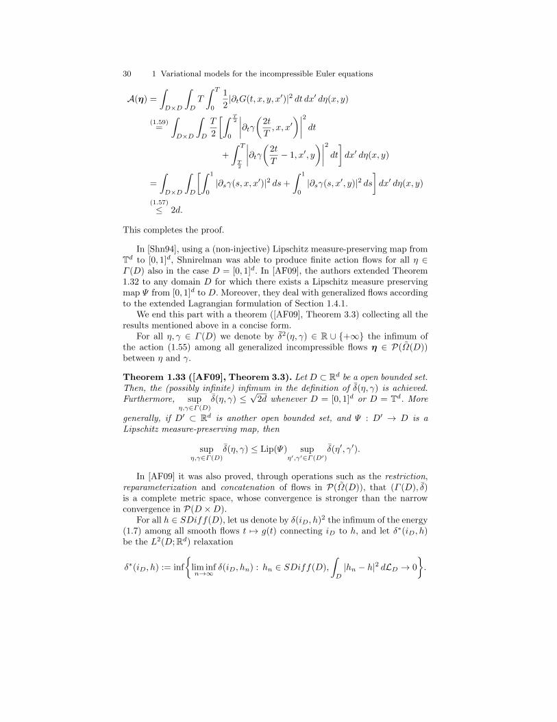
30 1 Variational models for the incompressible Euler equations
A(η) =
∫D×D
∫D
T
∫ T
0
1
2|∂tG(t, x, y, x′)|2 dt dx′ dη(x, y)
(1.59)=
∫D×D
∫D
T
2
[∫ T2
0
∣∣∣∣∂tγ(2t
T, x, x′
)∣∣∣∣2 dt+
∫ T
T2
∣∣∣∣∂tγ(2t
T− 1, x′, y
)∣∣∣∣2 dt] dx′ dη(x, y)
=
∫D×D
∫D
[∫ 1
0
|∂sγ(s, x, x′)|2 ds+
∫ 1
0
|∂sγ(s, x′, y)|2 ds]dx′ dη(x, y)
(1.57)
≤ 2d.
This completes the proof.
In [Shn94], using a (non-injective) Lipschitz measure-preserving map fromTd to [0, 1]d, Shnirelman was able to produce finite action flows for all η ∈Γ (D) also in the case D = [0, 1]d. In [AF09], the authors extended Theorem1.32 to any domain D for which there exists a Lipschitz measure preservingmap Ψ from [0, 1]d to D. Moreover, they deal with generalized flows accordingto the extended Lagrangian formulation of Section 1.4.1.
We end this part with a theorem ([AF09], Theorem 3.3) collecting all theresults mentioned above in a concise form.
For all η, γ ∈ Γ (D) we denote by δ2(η, γ) ∈ R ∪ +∞ the infimum ofthe action (1.55) among all generalized incompressible flows η ∈ P(Ω(D))between η and γ.
Theorem 1.33 ([AF09], Theorem 3.3). Let D ⊂ Rd be a open bounded set.Then, the (possibly infinite) infimum in the definition of δ(η, γ) is achieved.Furthermore, sup
η,γ∈Γ (D)
δ(η, γ) ≤√
2d whenever D = [0, 1]d or D = Td. More
generally, if D′ ⊂ Rd is another open bounded set, and Ψ : D′ → D is aLipschitz measure-preserving map, then
supη,γ∈Γ (D)
δ(η, γ) ≤ Lip(Ψ) supη′,γ′∈Γ (D′)
δ(η′, γ′).
In [AF09] it was also proved, through operations such as the restriction,reparameterization and concatenation of flows in P(Ω(D)), that (Γ (D), δ)is a complete metric space, whose convergence is stronger than the narrowconvergence in P(D ×D).
For all h ∈ SDiff(D), let us denote by δ(iD, h)2 the infimum of the energy(1.7) among all smooth flows t 7→ g(t) connecting iD to h, and let δ∗(iD, h)be the L2(D;Rd) relaxation
δ∗(iD, h) := inf
lim infn→∞
δ(iD, hn) : hn ∈ SDiff(D),
∫D
|hn − h|2 dLD → 0
.

1.4 Generalized incompressible flows 31
By (1.49) and the lower semicontinuity of δ with respect to narrow conver-gence, we have that
δ((iD × iD)]LD, (iD × h)]LD
)≤ δ∗(iD, h). (1.61)
In the case D = [0, 1]d, d ≥ 3, Shnirelman [Shn94] proved that the equalityin (1.61) holds. In [AF09] it is shown that, if d ≥ 3, the gap phenomenon stilldoes not occur even when non-deterministic final data are considered (i.e.,when considering as final configuration a plan γ ∈ Γ (D) instead of a maph ∈ S(D)). Hence, the strict inequality may hold only if d = 2 ([Shn94]).
1.4.3 Consistency with classical solutions
A natural question is whether the notion of action minimizing generalizedincompressible flow –whose existence has been proved in Section 1.4.2– isconsistent with the one of classical solution of the ODE (1.38).
The answer, provided by Brenier in [Bre89], states that whenever a gen-eralized flow satisfies the incompressibility constraint and is concentrated onsolutions of the ODE (1.38) for a sufficiently regular pressure field p, then itis a minimizer of the action (1.54) for small times.
More precisely, we have the following result:
Theorem 1.34 ([Bre89], Theorem 5.1). Let η ∈ Γ (D), and let η ∈P(Ω(D)) be a generalized incompressible flow compatible with η such that
ω(t) = −∇p(t, ω(t)), for η-a.e. ω ∈ Ω(D), (1.62)
where p : [0, T ] ×D → R is continuously differentiable with respect to x andsatisfies
T 2 sup(t,x)∈(0,T )×D
∇2xp(t, x) ≤ π2Id (1.63)
in the sense of distributions and symmetric matrices.Then η solves Problem 1.28 among all incompressible flows compatible
with η.Moreover, if the inequality (1.63) is strict, then η is the unique minimizer
and has the following deterministic property: η-almost surely, two paths ω andω′ satisfying both ω(0) = ω′(0) and ω(T ) = ω′(T ) are equal.
We notice that the above result holds also without the C1 assumption onp: indeed (1.63) implies that p is Lipschitz continuous with respect to x,and using that Lipschitz functions are differentiable LD-a.e. one can easilygeneralize the above result to this more general situation. However, in order toavoid extra technicalities, we have decided to state the result in this simplifiedform.
The following corollary, which is a direct consequence of Theorem 1.34,deals with the particular case of deterministic generalized flows induced byorientation and measure-preserving diffeomorphisms.
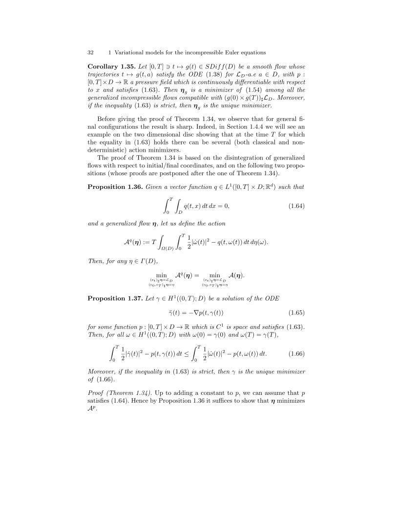
32 1 Variational models for the incompressible Euler equations
Corollary 1.35. Let [0, T ] 3 t 7→ g(t) ∈ SDiff(D) be a smooth flow whosetrajectories t 7→ g(t, a) satisfy the ODE (1.38) for LD-a.e a ∈ D, with p :[0, T ]×D → R a pressure field which is continuously differentiable with respectto x and satisfies (1.63). Then ηg is a minimizer of (1.54) among all thegeneralized incompressible flows compatible with (g(0)× g(T ))]LD. Moreover,if the inequality (1.63) is strict, then ηg is the unique minimizer.
Before giving the proof of Theorem 1.34, we observe that for general fi-nal configurations the result is sharp. Indeed, in Section 1.4.4 we will see anexample on the two dimensional disc showing that at the time T for whichthe equality in (1.63) holds there can be several (both classical and non-deterministic) action minimizers.
The proof of Theorem 1.34 is based on the disintegration of generalizedflows with respect to initial/final coordinates, and on the following two propo-sitions (whose proofs are postponed after the one of Theorem 1.34).
Proposition 1.36. Given a vector function q ∈ L1([0, T ]×D;Rd) such that∫ T
0
∫D
q(t, x) dt dx = 0, (1.64)
and a generalized flow η, let us define the action
Aq(η) := T
∫Ω(D)
∫ T
0
1
2|ω(t)|2 − q(t, ω(t)) dt dη(ω).
Then, for any η ∈ Γ (D),
min(et)]η=LD
(e0,eT )]η=η
Aq(η) = min(et)]η=LD
(e0,eT )]η=η
A(η).
Proposition 1.37. Let γ ∈ H1((0, T );D) be a solution of the ODE
γ(t) = −∇p(t, γ(t)) (1.65)
for some function p : [0, T ]×D → R which is C1 is space and satisfies (1.63).Then, for all ω ∈ H1((0, T );D) with ω(0) = γ(0) and ω(T ) = γ(T ),∫ T
0
1
2|γ(t)|2 − p(t, γ(t)) dt ≤
∫ T
0
1
2|ω(t)|2 − p(t, ω(t)) dt. (1.66)
Moreover, if the inequality in (1.63) is strict, then γ is the unique minimizerof (1.66).
Proof (Theorem 1.34). Up to adding a constant to p, we can assume that psatisfies (1.64). Hence by Proposition 1.36 it suffices to show that η minimizesAp.
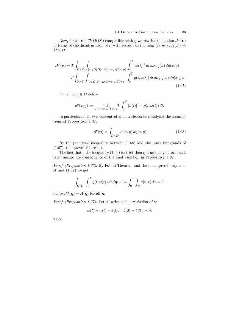
1.4 Generalized incompressible flows 33
Now, for all ν ∈ P(Ω(D)) compatible with η we rewrite the action Ap(ν)in terms of the disintegration of ν with respect to the map (e0, eT ) : Ω(D)→D ×D:
Ap(ν) = T
∫D×D
∫ω∈Ω(D):ω(0)=x,ω(T )=y
∫ T
0
|ω(t)|2 dt dνx,y(ω) dη(x, y)
− T∫D×D
∫ω∈Ω(D):ω(0)=x,ω(T )=y
∫ T
0
p(t, ω(t)) dt dνx,y(ω) dη(x, y).
(1.67)
For all x, y ∈ D define
ap(x, y) := infω(0)=x, ω(T )=y
T
∫ T
0
|ω(t)|2 − p(t, ω(t)) dt.
In particular, since η is concentrated on trajectories satisfying the assump-tions of Proposition 1.37,
Ap(η) =
∫D×D
ap(x, y) dη(x, y) (1.68)
By the pointwise inequality between (1.68) and the inner integrands of(1.67), this proves the result.
The fact that if the inequality (1.63) is strict then η is uniquely determined,is an immediate consequence of the final assertion in Proposition 1.37.
Proof (Proposition 1.36). By Fubini Theorem and the incompressibility con-straint (1.52) we get∫
Ω(D)
∫ T
0
q(t, ω(t)) dt dη(ω) =
∫ T
0
∫D
q(t, x) dx = 0,
hence Aq(η) = A(η) for all η.
Proof (Proposition 1.37). Let us write ω as a variation of γ:
ω(t) = γ(t) + δ(t), δ(0) = δ(T ) = 0.
Then

34 1 Variational models for the incompressible Euler equations∫ T
0
1
2|ω|2 − p(t, ω) dt =
∫ T
0
1
2|γ + δ|2 − p(t, γ + δ) dt
=
∫ T
0
1
2|γ|2 − p(t, γ) dt+
∫ T
0
δ · γ dt
+
∫ T
0
1
2|δ|2 dt+
∫ T
0
p(t, γ)− p(t, δ + γ) dt
=
∫ T
0
1
2|γ|2 − p(t, γ) dt+
∫ T
0
1
2|δ|2 dt
−∫ T
0
(p(t, γ + δ)− p(t, γ)− δ · ∇p(t, γ)
)dt, (1.69)
where the last equality is obtained integrating by parts the term∫δγ and
using (1.65). Now, thanks to (1.63) we notice that, for any t ∈ [0, T ],
p(t, γ(t) + δ(t))− p(t, γ(t))− δ(t) · ∇p(t, γ(t)) ≤ π2
2T 2|δ(t)|2. (1.70)
Moreover, by the Poincare inequality,
T 2
π2
∫ T
0
|δ|2 dt ≥∫ T
0
|δ|2 dt. (1.71)
(A simple way to prove such inequality is to use Fourier series.) Hence, sub-stituting (1.70) and (1.71) in (1.69), we get that t 7→ γ(t) is a minimizer, andit is the unique one in case of strict inequality in (1.63).
1.4.4 A two dimensional non-uniqueness example
In this section we discuss a non-uniqueness example of minimal generalizedflows in two dimensions, first put forward in [Bre89] and then further investi-gated in [BFS08].
Let D = B1(0) ⊂ R2 be the two dimensional unit disc and consider theminimization Problem 1.28 among all generalized incompressible flows con-necting iD to −iD at time T = π.
It is easy to see that the generalized incompressible flows ηg± inducedrespectively by the clockwise and counterclockwise rotations of angle t ∈ [0, π],
g±(t, a) := (a1 cos t∓ a2 sin t,±a1 sin t+ a2 cos t),
connect iD to −iD at time T = π and are concentrated on solutions of theODE
x(t) = −x(t). (1.72)
Notice that (1.72) corresponds to the “geodesic equation” (1.62) for thesmooth pressure field p(t, x) = 1
2 |x|2. Hence, since for such p (1.63) is satisfied

1.4 Generalized incompressible flows 35
for any T ≤ π, one can apply the consistency result of Theorem 1.34 anddeduce that both ηg+
and ηg− are minimizers of the action (1.54). Observethat, again by Theorem 1.34, for any time T < π the flow ηg+
(resp. ηg−) isthe unique minimizer of Problem 1.28 between iD and g+(T, ·) (resp. g−(T, ·)).
However, as noticed by Brenier in [Bre89], the loss of uniqueness at timeT = π is not limited to the previous examples but it is also due to theexistence of non-deterministic optimal generalized flows. Thanks to the resultsof Section 1.4.3, to obtain such minimizers it is sufficient to find generalizedincompressible flows on D which are concentrated – as ηg±– on solutions of(1.72). The example provided by Brenier is obtained considering the familyof minimizing curves ωx,θ connecting x to −x defined by
ωx,θ(t) := x cos t+√
1− |x|2(cos θ, sin θ) sin t, θ ∈ (0, 2π)
and taking
η :=1
2πωx,θ]
(LD(dx)× L1x[0, 2π](dθ)
).
Intuitively speaking, this non-deterministic flow spreads each particle of thefluid uniformly in all directions, along minimal geodesics for the augmentedenergy functional ω 7→
∫ π0
12 |ω(t)|2 − p(t, ω(t)) dt.
In [BFS08], Bernot, Figalli, and Santambrogio resumed Brenier’s exampleand constructed a rich set of new solutions to Problem 1.28 in this setting.Moreover, they provided also with a quite general characterization of thepossible minimizers.
With respect to Brenier’s original work [Bre89], the main additional infor-mation on the problem which is available to the authors of [BFS08] is the factthat being concentrated on solutions of the ODE (1.72) is not only sufficientbut also necessary for a generalized incompressible flow to be a minimizer.Indeed, by the analysis of the general Problem 1.28 carried out in [Bre93],[Bre99], [AF08], and [AF09] (see Section 1.5), it turns out that the pressurefield p(t, x) = 1
2 |x|2 is common to all the optimal generalized flows connect-
ing iD to −iD. More precisely, as we will see in Theorem 1.40, the pressurearises as a (unique, up to time dependent distributions) Lagrange multiplierfor the incompressibility constraint in the minimization Problem 1.28 withfixed initial and final configurations (given in this case by ±iD).
Therefore, the problem of finding and then characterizing the solutions ofProblem 1.28 in this case can be reformulated in the following way: The basicobservation is that, being solutions of the ODE (1.72), the trajectories of theflow are uniquely determined by their initial position and velocity. Hence (seeLemma 2.3 of [BFS08]), denoting by t 7→ Φ(t, x, v) ∈ R2 the unique integralcurve of (1.72) starting from x ∈ B1 with velocity v ∈ R2, any generalizedflow is optimal if and only if it is of the form
ηµ = Φ]µ,
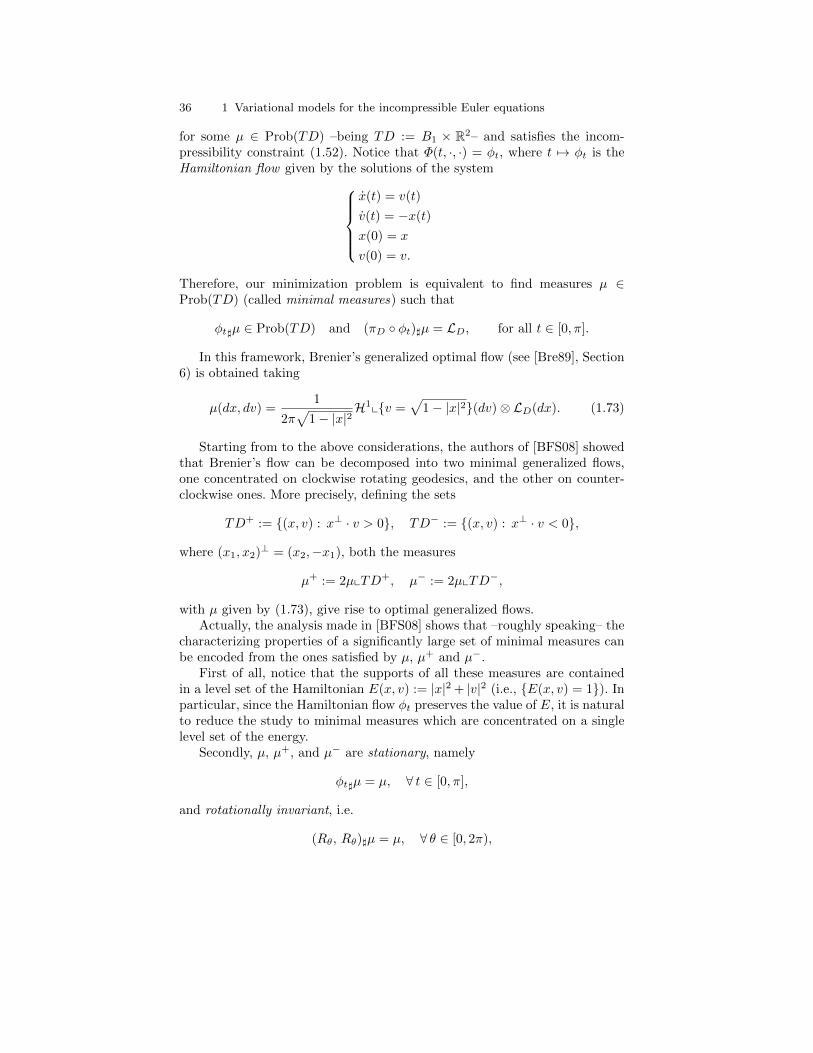
36 1 Variational models for the incompressible Euler equations
for some µ ∈ Prob(TD) –being TD := B1 × R2– and satisfies the incom-pressibility constraint (1.52). Notice that Φ(t, ·, ·) = φt, where t 7→ φt is theHamiltonian flow given by the solutions of the system
x(t) = v(t)
v(t) = −x(t)
x(0) = x
v(0) = v.
Therefore, our minimization problem is equivalent to find measures µ ∈Prob(TD) (called minimal measures) such that
φt]µ ∈ Prob(TD) and (πD φt)]µ = LD, for all t ∈ [0, π].
In this framework, Brenier’s generalized optimal flow (see [Bre89], Section6) is obtained taking
µ(dx, dv) =1
2π√
1− |x|2H1xv =
√1− |x|2(dv)⊗ LD(dx). (1.73)
Starting from to the above considerations, the authors of [BFS08] showedthat Brenier’s flow can be decomposed into two minimal generalized flows,one concentrated on clockwise rotating geodesics, and the other on counter-clockwise ones. More precisely, defining the sets
TD+ := (x, v) : x⊥ · v > 0, TD− := (x, v) : x⊥ · v < 0,
where (x1, x2)⊥ = (x2,−x1), both the measures
µ+ := 2µxTD+, µ− := 2µxTD−,
with µ given by (1.73), give rise to optimal generalized flows.Actually, the analysis made in [BFS08] shows that –roughly speaking– the
characterizing properties of a significantly large set of minimal measures canbe encoded from the ones satisfied by µ, µ+ and µ−.
First of all, notice that the supports of all these measures are containedin a level set of the Hamiltonian E(x, v) := |x|2 + |v|2 (i.e., E(x, v) = 1). Inparticular, since the Hamiltonian flow φt preserves the value of E, it is naturalto reduce the study to minimal measures which are concentrated on a singlelevel set of the energy.
Secondly, µ, µ+, and µ− are stationary, namely
φt]µ = µ, ∀ t ∈ [0, π],
and rotationally invariant, i.e.
(Rθ, Rθ)]µ = µ, ∀ θ ∈ [0, 2π),
1.5 The pressure field 37
being Rθ : R2 → R2 the counterclockwise rotation of angle θ.Having these properties in mind, the authors of [BFS08] proved the follow-
ing result, D being now either a disc or an annulus centered at the origin (notethat solutions in the disc can always be constructed as convex combinationsof solutions in disjoint annuli, so it is important to understand also the casewhen D is an annulus):
1. There is only one rotationally invariant clockwise (resp. counterclockwise)minimal measure µ that is concentrated on “the appropriate” energy levelE(x, v) = K (see Section 4.2 of [BFS08]);
2. There is only one stationary clockwise (resp. counterclockwise) mini-mal measure µ that is concentrated on “the appropriate” energy levelE(x, v) = K, and in particular this measure is rotationally invariant(see Section 4.3 of [BFS08]).
Without entering into the details, we just observe that, from the dimensionalpoint of view, the results are in accordance with the uniqueness of generalizedincompressible flows in dimension 1 (i.e., D = [−1, 1]) proved in [BFS08]. In-deed, in the 1-dimensional setting, the phase space is 2-dimensional, and inthis case the authors can prove uniqueness. Analogously, the “submanifold”of TB1 (which is 4-dimensional) defined by the energy constraint and the sta-tionarity (resp. the rotational invariance) of the measures is two dimensional,so it is natural to expect uniqueness there. However, as the results mentionedabove show, with respect to 1-dimensional case, in order to ensure unique-ness one still has to fix the degree of freedom given by the orientation of thetrajectories.
It is an open question whether there exist minimal measures which are notrotationally invariant. Finally, we refer to Remark 1.42 in Section 1.5.2 for therelation between the minimizing generalized flows constructed in [BFS08] andthe weak distributional solutions of the Euler equations defined in Section 1.2.
1.5 The pressure field
In the examples of Section 1.4.4 we have seen that, even for smooth finalconfigurations, action minimizing generalized incompressible flows may notbe unique. However, in all the examples, the minimizing flows with the samefinal configuration shared the same pressure. The aim of this section is toshow that this is not a coincidence, but a general fact.
Indeed, as shown by Brenier in [Bre93], for all the solutions of Problem1.28 which are compatible with the same configuration η ∈ Γ (D) there existsa unique, up to time dependent constants, pressure field. As will be shownbelow, such pressure field is a distribution arising as a Lagrange multiplier forthe incompressibility constraint when considering the action over the largerclass of almost-incompressible generalized flows.

38 1 Variational models for the incompressible Euler equations
1.5.1 The pressure as a Lagrange multiplier
By the invariance of the action under time reparameterization, from now onwe assume without loss of generality that T = 1. Moreover, in order to avoidarguments aiming at controlling the behaviour of generalized flows near theboundary, we assume that D = Td. Henceforth, D satisfies the assumptionsof Theorem 1.33 for the existence of minimizers of the action (1.54).
For all η ∈ Γ (D), define
A∗η := infA(η) : η ∈ P(Ω(D)), η0,1 = η
.
Definition 1.38 (Almost-incompressible flows). A generalized flow ν ∈P(Ω(D)) is almost-incompressible if there exists a smooth strictly positivefunction ρ : [0, 1]×D → R+ such that
νt = ρ(t, ·)LD, ∀ t ∈ [0, 1]
and
‖ρ− 1‖C1([0,1]×D) ≤1
2.
We call ρ = ρν the density field associated to ν.
Proposition 1.39 ([Bre93], Proposition 2.1). There exist ε0 ∈[0, 1
2 ) andc′ > 0 such that, for all smooth positive functions ρ : [0, 1]×D → R+ satisfyingρ(0, ·) = ρ(1, ·) = 1 and∫
D
ρ(t, x) dx = 1 ∀ t ∈ [0, 1], ‖ρ− 1‖C1([0,1]×D) ≤ ε0,
one can construct a Lipschitz continuous family of diffeomorphisms [0, 1] 3t 7→ γ(t, ·) on D, with γ(0, ·) = γ(1, ·) = iD, and
det∇xγ−1(t, x) = ρ(t, x), ∀ t ∈ [0, 1], x ∈ D.
Moreover, for each generalized incompressible flow η such that A(η) < +∞,the image measure of η through the mapping
Ω(D) 3 ω =(t 7→ ω(t)
)7→ ωγ =
(t 7→ γ(t, ω(t))
)∈ Ω(D)
defines an almost-incompressible flow ν := ηγ satisfying ρν = ρ, ν0,1 = η0,1,and
A(ν) ≤ A(η) + c′‖ρ− 1‖C1(1 +A(η)).
Theorem 1.40 ([Bre93], Theorem 1.1). For all η ∈ Γ (D) there existsp ∈ [C1
0 ([0, 1]×D)]∗ such that
〈p, ρν − 1〉 ≤ A(ν)−A∗η, (1.74)
for all almost-incompressible flows ν compatible with η.

1.5 The pressure field 39
Observe that, if ν satisfies the assumptions of Theorem 1.40, then ρν(0) =ρν(1) = 1. In particular, the duality bracket in the left-hand side of (1.74)is well defined. Here we report a simplified proof of Theorem 1.40 given byAmbrosio and Figalli in Theorem 6.2 of [AF09].
Proof (Theorem 1.40).Let C be the closed convex set
C :=
ρ ∈ C1([0, 1]×D) : ‖ρ− 1‖C1([0,1]×D) ≤
1
2, ρ(0, ·) = ρ(1, ·) = 1
and let us define the function φ : C1([0, 1]×D)→ R+ ∪ +∞,
φ(ρ) :=
infA(ν) : ρν = ρ and ν0,1 = η if ρ ∈ C+∞ otherwise.
Notice that φ(1) = A∗η. It is easy to check that φ is convex and lower semi-continuous on C1([0, 1] × D). Now we prove that φ has bounded slope at 1,namely
lim supρ→1
(φ(1)− φ(ρ))+
‖ρ− 1‖C1
< +∞. (1.75)
Indeed, if (1.75) holds, then applying the Hahn-Banach Theorem it fol-lows that the subdifferential of φ at 1 is nonempty, namely there existsp ∈ [C1
0 ([0, 1]×D)]∗ such that
〈p, ρ− 1〉 ≤ φ(ρ)− φ(1),
which is equivalent to (1.74).In order to prove (1.75) we observe that, given any smooth and positive
ρ as in Proposition 1.39, for all incompressible flows η connecting iD to η wecan find an almost incompressible flow ν with density field ρ, still connectingiD to η and satisfying
A(ν) ≤ A(η) + c′‖ρ− 1‖C1(1 +A(η)).
In particular, if η is a minimizer of the action, for any ρ is a C1-neighborhoodof 1 we get
φ(ρ) ≤ φ(1) + c′‖ρ− 1‖C1(1 + φ(1)),
which proves (1.75).
1.5.2 Uniqueness
Thanks to Theorem 1.40 one can now perform first variations of the actionfunctional A among almost-incompressible flows. Exploiting this fact, Brenierproved in [Bre93] that the pressure field is uniquely determined, up to timedependent distributions:
40 1 Variational models for the incompressible Euler equations
Theorem 1.41 ([Bre93], Section 7). For all generalized incompressibleflows η such that A(η) = A∗η, define the vector-valued measures
vηt LD = et](ωη), (vη ⊗ vη)tLD = et](ω ⊗ ωη). (1.76)
Then, for all p satisfying (1.74),
∂tvηt + div (vη ⊗ vη)t +∇p = 0 (1.77)
in the weak distributional sense. As a consequence, p is uniquely determinedup to time dependent distributions.
Proof. We perturb η as follows: let w : (0, 1)×D → R be a smooth compactlysupported vector field such that w(0, ·) = w(1, ·) = 0, and for ε ≥ 0 smalldefine the flow map
d
dεXt(ε, x) = w(t,Xt(ε, x)), Xt(0, x) = x.
Let Φε : Ω(D)→ Ω(D) denote the family of diffeomorphisms
Φε(ω(t)) = Xt(ε, ω(t)).
Then the density fields ρε = ρηε associated to ηε := Φε]η satisfy
d
dερε(t, x) + div (w(t, x)ρε(t, x)) = 0, ∀ t ∈ [0, 1]. (1.78)
Hence, if ε is sufficiently small, ηε is an almost-incompressible flow, and wehave
A(ηε)−A(η)
ε=
1
2ε
∫Ω(D)
∫ 1
0
∣∣∣∣ ddtΦε(ω(t))
∣∣∣∣2 − |ω(t)|2 dt dη(ω). (1.79)
Now, applying (1.74) and (1.78) to the left-hand side of (1.79), and thanks tothe fact that η is concentrated on H1((0, 1);D), we can let ε → 0+ in (1.79)and use (1.74) to obtain
−〈p,divw〉 ≤∫ 1
0
∫Ω(D)
ω(t) · ddt
[w(t, ω(t))
]dη(ω) dt
=
∫ 1
0
∫Ω(D)
ω(t) · ∂tw(t, ω(t)) + (ω(t) · ∇)w(t, ω(t)) · ω(t) dη(ω) dt.
(1.80)
Replacing w with −w, we deduce that equality in (1.80) holds.Finally, defining vη and (vη ⊗ vη) as in (1.76), by the arbitrariness of w
(1.80) is equivalent to (1.77).

1.5 The pressure field 41
Remark 1.42. Notice that vη is not a distributional solution of Euler, since ingeneral
(vη ⊗ vη) 6= vη ⊗ vη. (1.81)
However it is interesting to observe that, for the minimizing flows of theproblem considered in Section 1.4.4 which have been constructed in [BFS08],the difference of the two terms in (1.81) is a gradient. Hence, in that case,one can find true distributional solutions of (1.1) replacing the “microscopic”pressure field p with a new “macroscopic” one.
1.5.3 An Eulerian-Lagrangian formulation
In this section we present a second variational relaxation of the least actionprinciple (1.7). This formulation was introduced by Brenier in [Bre99] to de-scribe the limits of certain approximate solutions to Problem 1.1. Comparedto the Lagrangian model, the main advantage of this one consists in the factthat it allows to prove important regularity estimates on the pressure (1.74)([Bre99], [AF08]) which are crucial to derive necessary and sufficient condi-tions for optimality of generalized incompressible flows ([AF09]).
Let us assume with no loss of generality that T = 1, and let η = ηa ⊗dLD(a) ∈ Γ (D), γ = γa ⊗ dLD(a) ∈ Γ (D) be a pair of initial and finalconfigurations. Then consider the distributional solutions of the continuityequation
∂tct,a +∇ · (vt,act,a) = 0, in D′((0, 1)×D), for LD-a.e. a ∈ D, (1.82)
with the initial and final conditions
c0,a = ηa, c1,a = γa, for LD-a.e. a ∈ D. (1.83)
Defining the measures
c(dt, dx, da) := ct,a ⊗ (dt× dLD(a)), ct(dx, da) := ct,a ⊗ dLD(a) (1.84)
and the vector fieldv(t, x, a) := vt,a(x),
we observe that (1.82) is equivalent to
d
dt
∫D×D
φ(x, a) dct(x, a) =
∫D×D
〈∇xφ(x, a), v(t, x, a)〉 dct(x, a) (1.85)
for all φ ∈ Cb(D×D) which are continuously differentiable with respect to x.Then one studies the following:
Problem 1.43. Minimize the action
A(c, v) :=
∫ 1
0
∫D×D
1
2|v(t, x, a)|2 dct(x, a) dt (1.86)
42 1 Variational models for the incompressible Euler equations
among all couples (c, v) satisfying (1.82), (1.83), and the incompressibilityconstraint ∫
D
ct,a dLD(a) = LD, for all t ∈ [0, 1]. (1.87)
Remark 1.44. According to [BB00], the minimization of (1.86) without theglobal constraint (1.87) would give the optimal transportation problem (withquadratic cost) between η and γ.
The existence of minimizers was proved by standard compactness andsemicontinuity arguments in [Bre99]. This variational model is said to be ofEulerian-Lagrangian type since it contains two state variables (a, x) ∈ D×D,a representing the initial position of the fluid particles (Lagrangian coordinate)and x their actual position (Eulerian coordinate), and vt(x, a), which is the“average” velocity field of all particles which start from a and are at positionx at time t.
Remark 1.45. As noticed in [Bre99], to each minimizer (c, v) of Problem 1.43one can associate a measure-valued solution ν in the sense of DiPerna andMajda (see Definition 1.18) by setting∫
[0,1]×D×Rdf(t, x, ξ) dν(t, x, ξ) :=
∫[0,1]×D×D
f(t, x, v(t, x, a)) dc(t, x, a),
for all f ∈ C([0, 1]×D × Rd) with at most quadratic growth as ξ →∞.
The equivalence between Problem 1.43 and the extended Lagrangian for-mulation in Problem 1.28 was proved by Ambrosio and Figalli:
Theorem 1.46 ([AF09], Theorem 4.1). For all η, γ ∈ Γ (D),
minηA(η) = min
c,vA(c, v),
where η are the generalized incompressible flows connecting η to γ, and c, vsatisfy (1.82), (1.83), and (1.87). Moreover, every action minimizing general-ized incompressible flow η connecting η to γ induces a minimizer (c, v) of theEulerian-Lagrangian model and satisfies, for L1-a.e. t ∈ [0, 1], the condition
ω(t) = vt,a(ω(t)), for η-a.e. (ω, a).
Here we give only a sketch of the proof, mainly in order to understand therelationships between the configuration spaces of the two formulations.
Proof (Theorem 1.46).On the one hand, one can check that the correspondence
η 7→ (cηt,a, vηt,a) with cηt,a := (et)]ηa, cηt,av
ηt,a := (et)](ωηa)

1.6 Necessary and sufficient conditions for optimality 43
maps generalized incompressible flows η ∈ P(Ω(D)) connecting η to γ intocouples (cη, vη) satisfying (1.82), (1.83), (1.87), and∫
D
|vηt,a|2 dcηt,a ≤
∫Ω(D)
|ω(t)|2 dηa(ω), ∀ t ∈ [0, 1]. (1.88)
Hence, integrating (1.88) with respect to a ∈ D and t ∈ [0, 1] one hasA(cη, vη) ≤ A(η).
To show the reverse inequality one uses the following theorem with µt =ct,a (see [AGS05], Theorem 8.2.1):
Theorem 1.47 (Superposition principle). Assume that D ⊂ Rm is acompact set and that [0, 1] 3 t 7→ µt ∈ P(D) is a narrowly continuous so-lution of the continuity equation
∂µt +∇ · (vtµt) = 0
for some vector field v ∈ L1([0, 1];L2(Rd, µt)). Then there exists ν ∈ P(Ω(D))such that
(i) µt = (et)]ν, ∀ t ∈ [0, 1],
(ii)
∫Ω(D)
∫ 1
0
|ω(t)|2 dt dν(ω) ≤∫ 1
0
∫D
|v(t, x)|2 dx dt.
Remark 1.48. In the Eulerian-Lagrangian model the pressure field p is uniquelydetermined as a distribution, up to time dependent constants, by
∇p(t, x) = −∂t(∫
D
v(t, x, a) dct,x(a)
)−∇·
(∫D
v(t, x, a)⊗v(t, x, a) dct,x(a)
),
(1.89)where (c, v) is an optimal couple for Problem 1.43.
The use of the same letter to denote the pressure in both models is justifiedby the fact that the correspondence
η 7→ (cηt,a, vηt,a) with cηt,a := (et)]ηa, cηt,av
ηt,a := (et)](ωηa)
maps optimal solutions of the Lagrangian problem into optimal solutions ofthe Eulerian-Lagrangian one. Hence, since under this correspondence (1.89)reduces to (1.77), the two pressure fields must coincide.
1.6 Necessary and sufficient conditions for optimality
In this Section we deal (essentially without proofs) with necessary and suf-ficient conditions for minimality of generalized incompressible flows. As inSection 1.5 we assume that D = Td and we consider the extended minimiza-tion problem defined in Section 1.4.1 on the time interval [0, 1]. The study
44 1 Variational models for the incompressible Euler equations
carried in this section is due to Ambrosio and Figalli ([AF09]), with the ex-ception of Theorem 1.49 ([Bre99]). The main results are Theorems 1.54 and1.56, containing respectively the first and the second necessary condition, andfinally Theorem 1.57, showing that their joint validity is also sufficient foroptimality.
Theorem 1.40 (applied to the extended Lagrangian model) gives the fol-lowing necessary condition for action minimizing incompressible flows: letη ∈ P(Ω(Td)) be an optimal incompressible flow between η, γ ∈ Γ (Td), andconsider the augmented action
Ap(ν) :=
∫Ω(D)
∫ 1
0
1
2|ω(t)|2 dt dν(ω, a)− 〈p, ρν − 1〉, (1.90)
where p is given by Theorem 1.40. Then η minimizes (1.90) among all almost-incompressible flows connecting η to γ.
As in Theorem 1.34, one would like to evince from the minimization of theaugmented action (1.90) further necessary conditions for optimality whichcould be expressed in terms of the trajectories followed by the generalizedflows. However, if p was merely a distribution and not a function, it would beimpossible to compute its values along curves in Td. To reach this goal it hasbeen necessary to improve the regularity properties of p.
The first result concerning the regularity of the pressure was obtained byBrenier [Bre99] by means of the Eulerian-Lagrangian formulation describedin Section 1.5.3 (see Remark 1.48).
Theorem 1.49 ([Bre99], Theorem 1.2). For all η, γ ∈ Γ (Td), the distri-butional spatial derivatives ∂xipdi=1 of the distribution p given by Theorem1.40 belong to the space of locally finite measures Mloc((0, 1)× Td)).
However, the regularity obtained in Theorem 1.49 is still not sufficient todefine path functionals of the type
H1((0, T );Td) 3 γ 7→∫ T
0
1
2|γ(t)|2 − p(t, γ(t)) dt.
In [AF08], Brenier’s result was improved by Ambrosio and Figalli as fol-lows:
Theorem 1.50 ([AF08], Theorem 3.1 and Corollary 3.3). For allη, γ ∈ Γ (Td), let p be the distribution given by Theorem 1.40. Then ∂xip ∈L2
loc((0, 1)×M(Td)). In particular,
p ∈ L2loc((0, 1);BV (Td)) ⊂ L2
loc((0, 1);Ld/(d−1)(Td)). (1.91)
Thanks to (1.91) we have that p is a function, both in the time and spacevariables. Hence, one can try to derive from (1.90) some informations on thecurves followed by a minimizing flow η.
1.6 Necessary and sufficient conditions for optimality 45
Up to adding a time dependent constant, without loss of generality we canassume that ∫
Tdp(t, x) dx = 0, for a.e. t ∈ [0, 1]. (1.92)
Recall that, by Theorem 1.34 and Corollary 1.35, at least for short timeintervals any smooth solution of the Euler equations induces an incompressibleflow η such that η-a.e. ω ∈ Ω(Td) minimizes the Lagrangian action 1
2 |v|2 −
p(t, x).In order to generalize this kind of result to optimal generalized flows whose
pressure field p satisfies the properties of Theorem 1.50, one has to deal withthe following technical problems:
1. p is defined only dt× LTd -a.e.;
2. p might not be integrable with respect to t in a neighborhood of 0 and 1.
To solve 1, one chooses a particular representative of p in its equivalenceclass. A good choice is
p(t, x) := lim infε→0
pε(t, x) (1.93)
where, considering p(t, ·) as a 1-periodic function on Rd,
pε(t, x) := (2π)−d/2∫Rdp(t, x+ εy)e−|y|
2/2 dy.
Notice that pε(t, ·) is still 1-periodic and
(pε)ε′ = pε+ε′ . (1.94)
Observe that p = p at every Lebesgue point of p(t, ·), therefore p is a repre-sentative of p.
To deal with 2, one replaces the concept of minimizing curves of the La-grangian action with the one of locally minimizing curves, namely curves min-imizing the action on all time intervals [s, t] ⊂ (0, 1). Moreover, when definingwhich are the curves that are “admissible competitors” in the minimizationproblem, we need to avoid that such curves concentrate on regions wherep = +∞ for a set of times having positive measure. To prevent this fact, wefirst introduce the concept of maximal function.
Definition 1.51. For all f ∈ L1(Td), the maximal function of f is defined as
Mf(x) := supε>0
(2π)−d/2∫Rd|f |(t, x+ εy)e−|y|
2/2 dy.
In the rest of this section we will use the following facts: first, by (1.94)
Mfε = supε′>0
(|f |ε)ε′
= supε′|f |ε+ε′ ≤ sup
ε′′>0|f |ε′′ = Mf.
46 1 Variational models for the incompressible Euler equations
Moreover, by standard maximal inequalities one has
‖Mf‖Lp(Td) ≤ Cp‖f‖Lp(Td), for all p > 1.
Setting Mp(t, x) := Mp(t, ·), by Theorem 1.50 one gets that Mp ∈L2
loc((0, 1);Ld/(d−1)(Td)), so in particular
Mp ∈ L1loc((0, 1)× Td). (1.95)
The regularity of p expressed by (1.95) is the one that is needed to formulatethe first necessary condition in terms of minimal trajectories.
Definition 1.52 (q-minimizing paths). Let q : [0, 1] × Td → R satisfy(1.92). Fix ω ∈ H1((0, 1) × Td), and assume that Mq(τ, ω(τ)) ∈ L1((0, 1)).We say that ω is a q-minimizing path if∫ 1
0
1
2|ω(τ)|2 − q(τ, ω(τ)) dτ ≤
∫ 1
0
1
2|ω(τ) + δ(τ)|2 − q(τ, ω(τ) + δ(τ)) dτ,
for all δ ∈ H10 ((0, 1);Td) with Mq(τ, ω(τ) + δ(τ)) ∈ L1((0, 1)).
If we only have that Mq(τ, ω(τ)) ∈ L1loc((0, 1)), we say that ω is a locally
q-minimizing path if∫ t
s
1
2|ω(τ)|2 − q(τ, ω(τ)) dτ ≤
∫ t
s
1
2|ω(τ) + δ(τ)|2 − q(τ, ω(τ) + δ(τ)) dτ,
for all [s, t] ⊂ (0, 1) and for all δ ∈ H10 ((s, t);Td) with Mq(τ, ω(τ) + δ(τ)) ∈
L1((s, t)).
We observe that, when taking q = p, the integrability condition on Mp alongthe curve ω + δ is done exactly to avoid that the curve spend some “non-negligible time” in regions where p = +∞.
Remark 1.53. Observe that if η is incompressible, A(η) < +∞, and Mq ∈L1
(loc)((0, 1) × Td), then for all δ ∈ H10 ((0, 1);Td) the following holds: for η-
a.e. (ω, a),
Mq(τ, ω(τ) + δ(τ)) ∈ L1((0, 1)), (resp. L1((s, t)) for all [s, t] ⊂ (0, 1)).
Indeed, the incompressibility of η, Fubini Theorem, and the translation in-variance of the Lebesgue measure give∫
Ω(D)
∫J
Mq(τ, ω + δ) dη(ω, a) =
∫J
∫TdMq(τ, x+ δ(τ)) dx dτ
=
∫J
∫TdMq(τ, x) dx dτ < +∞
for all intervals J ⊂ (0, 1). This shows that the set of “admissible perturba-tions” is in some sense very large.

1.6 Necessary and sufficient conditions for optimality 47
The first necessary condition for optimality is expressed by the following:
Theorem 1.54 ([AF09], Theorem 6.8). Let η be an action-minimizing in-compressible generalized flow. Then η is concentrated on locally p-minimizingpaths, where p is the precise representative of the pressure field p defined in(1.93), and on p-minimizing paths if Mp ∈ L1((0, 1)× Td).
Remark 1.55. The fact that an optimal generalized flow η is concentrated onlocally action-minimizing paths should imply some further regularity prop-erties of these paths. In particular, exploiting that p is BV in the spatialvariable (see (1.91)) one may expect that η-a.e. path solves some weak formof the Euler-Lagrange equation. (In [FM] this question is addressed under theadditional assumption that p is Sobolev in the space variable.)
In order to state the second necessary condition we need some preliminarydefinition.
Given q ∈ L1([s, t]×Td) satisfying (1.92), define the cost cs,tq : Td ×Td →R ∪ +∞ of the q-minimal connection between x and y as
cs,tq (x, y) := inf
∫ t
s
1
2|ω(τ)|2−q(τ, ω(τ)) dτ : ω(s) = x, ω(t) = y,
Mq(τ, ω(τ)) ∈ L1((s, t))
, (1.96)
with the convention that cs,tq (x, y) = +∞ if there are no admissible curves ωbetween x and y.
Using this cost function, one can consider the optimal transport problem
Wcs,tq(µ1, µ2) = inf
∫Td×Td
cs,tq (x, y) dλ(x, y) : (π1)]λ = µ1, (π2)]λ = µ2,
(cs,tq )+ ∈ L1(λ)
, (1.97)
where again Wcs,tq(µ1, µ2) = +∞ if no admissible λ exists.
Notice that, in general, the existence of minimizers for (1.97) is not guar-anteed because the functions cs,tq may be not lower semicontinuous.
Choosing q = p|[s,t] , where p ∈ L1loc((0, 1)×Td) is the representative (1.93)
of the pressure field, we can state the second necessary condition for optimal-ity.
Theorem 1.56 ([AF09], Theorem 6.11). Let η be an optimal generalizedincompressible flow between η and γ ∈ Γ (Td). Then, for all [s, t] ⊂ (0, 1),Wcs,tp
(ηsa,ηta) < +∞ and the plan (es, et)]ηa is optimal, relative to the cost
cs,tp defined in (1.96), for LTd-a.e. a ∈ Td.

48 1 Variational models for the incompressible Euler equations
Roughly speaking, the above result says that an optimal generalized flownot only chooses to follow locally action-minimizing paths, but actually moreis true. In order to understand this second necessary condition, consider forinstance the following simple example: a particle starts from a and splits intotwo particles with equal mass, which at times s, t ∈ (0, 1) are respectivelyat positions a1(s), a2(s) and a1(t), a2(t). Then the optimal flow not only willjoin a1(s) to a1(t) (resp. a2(s) to a2(t)) using action-minimizing paths, butthe total cost is also minimized, i.e.
cs,tp (a1(s), a1(t)) + cs,tp (a2(s), a2(t)) ≤ cs,tp (a1(s), a2(t)) + cs,tp (a2(s), a1(t)).
We remark that this additional necessary condition is specific to the relaxedmodel, and it is empty if the flow is deterministic (that is, if the particles donot split).
Finally, the conditions given in Theorems 1.54 and 1.56 turns out to bealso sufficient for optimality.
Theorem 1.57 ([AF09], Theorem 6.12). Let η ∈ P(Ω(Td)) be a general-ized incompressible flow between η and γ ∈ Γ (Td), and assume that for somefunction q ∈ L1
loc((0, 1)× Td) satisfying (1.92) the following properties hold:
(a) Mq ∈ L1((0, 1)× Td) and η is concentrated on q-minimizing paths;
(b) the plan (e0, e1)]ηa is optimal, relative to the cost c0,1q defined in (1.96),
for LTd-a.e. a ∈ Td.
Then η is optimal and q is the unique pressure field. In addition, if (a) and(b) are replaced by:
(a′) Mq ∈ L1loc((0, 1)× Td) and η is concentrated on locally q-minimizing paths;
(b′) For all intervals [s, t] ⊂ (0, 1) the plan (es, et)]ηa is optimal, relative to
the cost cs,tq defined in (1.96), for LTd-a.e. a ∈ Td;
then the same conclusions hold.
References
[AF08] Ambrosio, L., Figalli, A.: On the regularity of the pressure field of Bre-nier’s weak solutions to incompressible Euler equations. Calc. Var. PartialDifferential Equations, 31 (2008), 497-509.
[AF09] Ambrosio, L., Figalli, A.: Geodesics in the space of measure-preservingmaps and plans. Arch. Ration. Mech. Anal., 194 (2009), no. 2, 421-462.
[AGS05] Ambrosio, L., Gigli, N., Savare, G.: Gradient flows in metric spaces and inthe Wasserstein space of probability measures. Lectures in Mathematics,ETH Zurich, Birkhauser, 2005.
[Arn66] Arnold, V.: Sur la geometrie differentielle des groupes de Lie de dimensioninfinie et ses applications a l’hydrodynamique des fluides parfaits. Ann.Inst. Fourier (Grenoble), 16 (1966), fasc. 1, 319-361.
[BB00] Benamou, J.-D.; Brenier, Y.: A computational fluid mechanics solution tothe Monge-Kantorovich mass transfer problem. Numer. Math., 84 (2000),no. 3, 375-393.
[BFS08] Bernot, M., Figalli, A., Santambrogio, F.: Generalized solutions for theEuler equations in one and two dimensions. J. Math. Pures Appl., 91(2008), no. 2, 137-155.
[BM02] Bertozzi, A. L., Majda, A. J.: Vorticity and incompressible flow. Vol. 27 ofCambridge Texts in Applied Mathematics. Cambridge Univessity Press,Cambridge, 2002.
[Bre89] Brenier, Y.: The least action principle and the related concept of general-ized flows for incompressible perfect fluids. J. Amer. Mat. Soc., 2 (1989),225-255.
[Bre91] Brenier, Y.: Polar factorization and monotone rearrangement of vector-valued functions. Comm. Pure Appl. Math., 44 (1991), no. 4, 375-417.
[Bre93] Brenier, Y.: The dual least action problem for an ideal, incompressiblefluid. Arch. Ration. Mech. Anal., 122 (1993), 323-351.
[Bre99] Brenier, Y.: Minimal geodesics on groups of volume-preserving maps andgeneralized solutions of the Euler equations. Comm. Pure Appl. Math.,52 (1999), 411-452.
[Bre08] Brenier, Y.: Generalized solutions and hydrostatic approximation of theEuler equations. Phys. D, 237 (2008), no. 14-17, 1982-1988.
50 References
[BDS11] Brenier, Y., De Lellis, C., Szekelyhidi, L.: Weak-strong uniqueness formeasure-valued solutions. Comm. Math. Phys., 305 (2011), no. 2, 351-361.
[BG03] Brenier, Y., Gangbo, W.: Lp approximation of maps by diffeomorphisms.Calc. Var. Partial Differential Equations, 16 (2003), no. 2, 147-164.
[DLS09] De Lellis, C., Szekelyhidi, L.: The Euler equations as a differential inclu-sion. Ann. of Math. (2), 170 (2009), no. 3, 1417-1436.
[DLS10] De Lellis, C., Szekelyhidi, L.: On admissibility criteria for weak solutionsof the Euler equations. Arch. Ration. Mech. Anal., 195 (2010), no. 1,225-260.
[Del91] Delort, J.M.: Existence de nappes de tourbillon en dimension deux(French) [Existence of vortex sheets in dimension two]. J. Amer. Math.Soc., 4 (1991), no. 3, 553-586.
[DiP85] DiPerna, R. J.: Measure-valued solutions to conservation laws. Arch. Ra-tion. Mech. Anal., 88 (1985), no. 3, 223-270.
[DiPM87] DiPerna, R. J., Majda, A. J.: Oscillations and concentrations in weaksolutions of the incompressible fluid equations. Comm. Math. Phys., 108(1987), no. 4, 667-689.
[EM70] Ebin, D.G., Marsden, J.: Groups of diffeomorphisms and the motion ofan ideal incompressible fluid. Ann. of Math. (2), 92 (1970), 102-163.
[FM] Figalli, A., Mandorino V.: Fine properties of minimizers of mechanical La-grangians with Sobolev potentials. Discrete Contin. Dyn. Syst., 31 (2011),no. 4, 1325-1346.
[Gun27] Gunther, N.: On the motion of fluid in a moving container. Izv. Akad.Nauk SSSR. Ser. Fiz.-Mat. 20 (1926), 1323-1348, 1503-1532; 21 (1927),621-556, 735-756, 1139-1162; 22 (1928), 9-30.
[Kat68] Kato, T.: On classical solutions of the two-dimensional non-stationaryEuler equation. Arch. Ration. Mech. Anal., 27 (1968), 188-200.
[Ler34] Leray, J.: Sur le mouvement d’un liquide visqueux emplissant l’espace.(French) Acta Math., 63 (1934), no. 1, 193-248.
[Lic25] Lichtenstein, L.: Uber einige Existenzprobleme der Hydrodynamik ho-mogener unzusammendruckbarer, reibunglosser Flussikeiten und dieHelmholtzschen Wirbelsaltze. Math. Zeit. 23 (1925), 89-154; 26 (1927),196-323, 387-415, 725; 32 (1930), 608.
[Li96] Lions, P.-L.: Mathematical topics in fluid mechanics. Vol. 1, Vol. 3 ofOxford Lecture Series in Mathematics and its Applications. New York:The Clarendon Press, Oxford University Press (1996).
[Sch93] Scheffer, V.: An inviscid flow with compact support in space-time. J.Geom. Anal., 3 (1993), no. 4, 343-401.
[Shn87] Shnirelman, A.I.: The geometry of the group of diffeomorphisms and thedynamics of an ideal incompressible fluid. (Russian) Mat. Sb. (N.S.), 128(170) (1985), no. 1, 82-109.
[Shn94] Shnirelman, A.I.: Generalized fluid flows, their approximation and appli-cations. Geom. Funct. Anal., 4 (1994), no. 5, 586-620.
[Shn97] Shnirelman, A.I.: On the nonuniqueness of weak solution of the Eulerequation. Comm. Pure Appl. Math., 50 (1997), no. 12, 1261-1286.
[Ste70] Stein, E.: Singular integrals and differentiability properties of functions.Princeton University Press, 1970.

References 51
[Tar79] Tartar, L.: Compensated compactness and applications to partial differ-ential equations. In: Nonlinear analysis and mechanics: Heriot-Watt Sym-posium, Vol. IV, pp. 136-212, Res. Notes in Math., 39, Pitman, Boston,Mass.-London, 1979.
[Tar83] Tartar, L.: The compensated compactness method applied to systems ofconservation laws. In: Systems of nonlinear partial differential equations(Oxford, 1982), 263-285, NATO Adv. Sci. Inst. Ser. C Math. Phys. Sci.,111, Reidel, Dordrecht, 1983.
[Tay96] Taylor, M. E.: Partial differential equations. III. Nonlinear equations. Ap-plied Mathematical Sciences, 117. Springer-Verlag, New York, 1996.
[Wol33] Wolibner, W.: Un theoreme sur l’existence du movement plan d’un flu-ide parfait, homogene, incompressible, pendant un temps infiniment long.Math. Zam., 37 (1933), 698-726.
[Yud63] Yudovich, V.I.: Nonstationary flow of an ideal incompressible liquid.Zhurn. Vych. Mat., 3 (1963), 1032-1066.
[Yud95] Yudovich, V.I. Uniqueness theorem for the basic nonstationary problem inthe dynamics of an ideal incompressible fluid. Math. Res. Lett., 2 (1995),no. 1, 27-38.