On Exact Conservation for the Euler Equationswith Complex Equations of State

J. W. Banks1,∗

1 Center for Applied Scientific Computing, Lawrence Livermore National Lab-oratory, Livermore, California, 94551

Abstract. Conservative numerical methods are often used for simulations of fluid flowsinvolving shocks and other jumps with the understanding that conservation guaranteesreasonable treatment near discontinuities. This is true in that convergent conservativeapproximations converge to weak solution and thus have the correct shock location.However, correct shock location results from any discretization whose violation of con-servation approaches zero as the mesh is refined. Here we investigate the case of theEuler equations for a single gas using the Jones-Wilkins-Lee (JWL) equation of state.We show that a quasi-conservative method can lead to physically realistic solutionswhich are devoid of spurious pressure oscillations. Furthermore, we demonstrate thatunder certain conditions, a quasi-conservative method can exhibit higher rates of con-vergence near shocks than a strictly conservative counterpart of the same formal order.

AMS subject classifications: 65N08, 35L60, 35L65, 76N15

Key words: Euler equations, complex EOS, JWL EOS, Godunov methods

1 Introduction

The use of conservative schemes for simulations of solutions to hyperbolic conservation lawsin the presence of discontinuities is ubiquitous. The reasons draw largely from the fact thatconvergent conservative schemes are known to converge to weak solutions in the presenceof shocks by the Lax-Wendroff theorem [1]. On the other hand, non-conservative schemescan converge to non-weak solutions which violate the integral conservation equations [2].However, weak solutions which violate physical properties, such as positivity of density orentropy satisfaction, are equally as troublesome as non-weak solutions and there is verylittle theory guaranteeing convergence for nonlinear systems to the appropriate “vanishingviscosity” solution (one notable exception is the random choice method of Glimm [3]). Itis interesting then that so much emphasis has been placed on exact conservation ratherthan rapid convergence to the relevant vanishing viscosity solution.

∗Corresponding author. Email addresses: banks20@llnl.gov (J.W. Banks)

http://www.global-sci.com/ Global Science Preprint

2

One prototypical physical system described by hyperbolic conservation laws is that ofgas dynamics. Here the governing system is the Euler equations and for cases where theequation of state is sufficiently nonlinear, issues relating to exact conservation rise verymuch to the surface. The classical realization of these problems is unphysical oscillations,particularly in the pressure, arising near material interfaces in multi-material flows [4–10].Somewhat less appreciated is the fact that the same type of behavior can be exhibited forsingle component flows with complicated equations of state [11].

The multi-component case has been studied extensively and many non-conservative orquasi-conservative schemes have been proposed and used to great effect in that context.Nonlinearities in the equation of state result when sharp material interfaces are smearedthrough the use of a capturing scheme. To remedy this, the paper by Quirk and Karni [5]for instance, relies on a non-conservative primitive formulation and adds source termswhich restore conservation where possible. Other choices that have been made includethe use of a hybrid approach that relies on the conservative update whenever possiblebut uses the primitive update near interfaces [4], conservative approximations which addsource terms to break conservation as required near material interfaces [9,10], and specialadvection rules for particular components of the equation of state [6, 7]. All of theseapproaches seek to realize physically realistic treatment of the material interface throughthe use of non-conservative schemes and rely on the fact that the poor behavior exhibitedby capturing schemes is limited to a small region about the material interface.

In [11] the authors show that poor behavior is not limited to material interfaces andproblems can occur for single component flows with sufficiently nonlinear equations ofstate. In that paper, the authors present a new numerical method to treat such flows.Their scheme relies on a specific class of Riemann solver, a specific equation of state, andin the end introduces special advection rules for the adiabatic exponent which amounts toa modification of the equation of state. Their approach does seems to have some efficacywhen it is applicable, but alterations of the equation of state can lead to inconsistentnumerical schemes and great care must be used. Without assurances that the numericalsystem is consistent with the original PDE as well as convergent, this scheme also facesobstacles in terms of application of the Lax-Wendroff theorem.

The state of matters then seems to be that the classical, that is to say consistent andconservative, schemes may produce physically unrealistic results; especially near contacts.As a result, even though some theoretical benefit is achieved through the use of fullyconservative schemes, they can produce approximations which are not useful and so mod-ifications to these schemes are developed. On one hand there is the class of schemes whichmodify the governing equations and thus risk inconsistency [11]. On the other hand thereis the class of schemes which modify conservation with the obvious associated risks [4–10].It is not at all clear that these approaches are entirely different and it may be the casethat the actual numerical approximations are quite similar.

In the current paper we will demonstrate the poor behavior of one particular classicalconservative scheme when applied to a simple Riemann problem with a single Jones-Wilkins-Lee (JWL) gas. The choice of the JWL equation of state is motivated by high

3

explosives applications, but many other real gas equations of state would exhibit similarbehavior. For this problem, the global convergence character of the solution is demon-strated to be dominated by the convergence character near the contact and somewhatsurprisingly the shock is seen to be incorrectly located by an increasing number of gridcells as the grid spacing is reduced. To contrast this, the quasi-conservative scheme of [9]is modified so that the non-conservative source term is active whenever the acoustic char-acteristic field is not dominant. This type of switching mechanism yields the property thatas the grid is refined, the error in energy conservation approaches zero. As a result, theapproximations approach a conservative solution and, because the method is consistent,the Lax-Wendroff theorem is applicable. We call such schemes quasi-conservative schemes.The primary benefits of this new scheme are its applicability to any equation of state, anyRiemann solver, and higher dimensions without the use of dimensional splitting. Interest-ingly, the new scheme is shown to produce more rapid convergence near the shock of theexample Riemann problem than a fully conservative counterpart. High convergence ratesmay be important in many applications. For instance in a reacting flow, stiff source termscan require highly accurate flow fields in order to faithfully reproduce the dynamics of thephysical system.

The remainder of this paper is organized as follows. Section 2 presents the governingequations including the JWL equation of state which we use. A solution strategy for theRiemann problem with general convex equations of state is presented in section 3. Thenumerical methods used in the paper are developed in section 4. Numerical results for theapplication of these schemes to a Riemann problem are presented in section 5. A morepractical example of the associated issues is presented in section 6 and concluding remarksare made in section 7.

2 Governing equations

The governing equations under consideration in this paper are the one-dimensional Eu-ler equations for a single component. These equations can be viewed as the system ofconservation laws

∂

∂tu+

∂

∂xf(u)=0, (2.1)

where

u=

ρρuρE

, f(u)=

ρuρu2+pu(ρE+p)

.

The variables have the usual meanings with ρ being the density, u the velocity, E the totalenergy per unit mass, and p the pressure. Here the total energy for the fluid is given by

E=e+1

2u2,

where e= e(ρ,p) is the specific internal energy which is specified through an equationof state (EOS). The equations are assumed to have been rendered dimensionless using

4

suitable scalings of the variables. For this work, emphasis is place on non-ideal equationsof state and a Jones-Wilkins-Lee (JWL) EOS is chosen. This EOS is given by

e(ρ,p)=pv

ω−F(v)+F(v0) (2.2)

where v= 1ρ and p are the specific volume and pressure respectively, and v0 is a reference

specific volume. Such an EOS is often encountered when modeling high explosives. The useof this specific EOS is not critical and is just one example where the associated problemsmight arise. This choice was made to make the discussion concrete, but other forms suchas Mie-Gruneisen, Van der Waals, or others could have been considered. In the JWLforms, ω is the Gruneisen coefficient, and F(v), the stiffening function, is given by

F(v)=A

(v

ω− 1

R1

)exp(−R1v)+B

(v

ω− 1

R2

)exp(−R2v), (2.3)

where A, B, R1 and R2 are constants for a given material [12]. Equation (2.2) representsthe mechanical EOS but the full JWL model involves a thermal equation of state as well.Both the mechanical and thermal equations might be considered when modeling mixturesof multiple materials for example, but for this single gas case the mechanical EOS issufficient. Notice that the JWL form in (2.2) and (2.3) includes as a special case the idealgas EOS when F(v)=0. For the simulations presented in this paper, the particular choicefor the EOS parameters is shown in table 1 which corresponds roughly to the solid usedfor some condensed-phase explosive models [12].

parameter A B R1 R2 ω v0

value 692.5067 −0.044776 11.3 1.13 0.8938 0.5

Table 1: Values for the parameter associated with the EOS (2.2).

3 Exact solution of Riemann problem with convex EOS

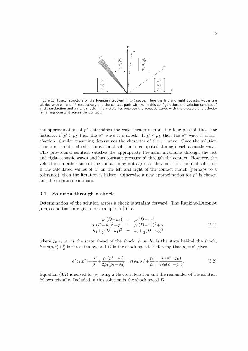
One particularly important solution to (2.1) is the solution of the Riemann problem. Theexact solution to the Riemann problem for convex EOS has been investigated for examplein [13–15] but it is useful to give a brief outline of a complete numerical strategy. Givenleft and right primitive states wL = [ρL,uL,pL]T and wR = [ρR,uR,pR]T respectively, thesolution consists of left and right acoustic waves and a center contact. Each acoustic wavecan be either a shock or rarefaction and thus there are four possible configurations. Onesuch configuration is shown schematically in figure 1. As in many previous works, the“star” superscript is used to denote the region between the two acoustic waves.

The solution strategy used here, which is similar to that discussed in [14] and [15],involves the solution of a nonlinear equation for the center pressure p∗. To ensure robust-ness of the solver, this is realized numerically as a bisection iteration. At each iteration,

5

t

x

u

c-

c+

ρ∗Lu∗

p∗

ρRuR

pR

ρLuL

pL

ρ∗Ru∗

p∗

Figure 1: Typical structure of the Riemann problem in x-t space. Here the left and right acoustic waves arelabeled with c− and c+ respectively and the contact path with u. In this configuration, the solution consists ofa left rarefaction and a right shock. The ∗-state lies between the acoustic waves with the pressure and velocityremaining constant across the contact.

the approximation of p∗ determines the wave structure from the four possibilities. Forinstance, if p∗>pL then the c− wave is a shock. If p∗≤ pL then the c− wave is a rar-efaction. Similar reasoning determines the character of the c+ wave. Once the solutionstructure is determined, a provisional solution is computed through each acoustic wave.This provisional solution satisfies the appropriate Riemann invariants through the leftand right acoustic waves and has constant pressure p∗ through the contact. However, thevelocities on either side of the contact may not agree as they must in the final solution.If the calculated values of u∗ on the left and right of the contact match (perhaps to atolerance), then the iteration is halted. Otherwise a new approximation for p∗ is chosenand the iteration continues.

3.1 Solution through a shock

Determination of the solution across a shock is straight forward. The Rankine-Hugoniotjump conditions are given for example in [16] as

ρ1(D−u1) = ρ0(D−u0)ρ1(D−u1)2+p1 = ρ0(D−u0)2+p0

h1+ 12(D−u1)2 = h0+ 1

2(D−u0)2(3.1)

where ρ0,u0,h0 is the state ahead of the shock, ρ1,u1,h1 is the state behind the shock,h=e(ρ,p)+ p

ρ is the enthalpy, and D is the shock speed. Enforcing that p1 =p∗ gives

e(ρ1,p∗)+

p∗

ρ1+ρ0(p∗−p0)

2ρ1(ρ1−ρ0)=e(ρ0,p0)+

p0

ρ0+ρ1(p∗−p0)

2ρ0(ρ1−ρ0). (3.2)

Equation (3.2) is solved for ρ1 using a Newton iteration and the remainder of the solutionfollows trivially. Included in this solution is the shock speed D.

6

3.2 Solution through a rarefaction

Numerical approximation through a rarefaction wave is somewhat more involved but con-ceptually straightforward. Rarefactions are isentropic implying that the sound speed adepends only on the density. Determination of the sound speed a will be discussed insection 3.3. This implies a2 = ∂p

∂ρ and so

∫[a(ρ,p(ρ))]2dρ=

∫dp. (3.3)

Starting from the state [ρ0,u0,p0]T , the solution is determined in a Runge-Kutta likestrategy [17]

pk+1≈pk−∆ρ

6

([a(ρk,p1)]2+2[a(ρk+1/2,p2)]2+2[a(ρk+1/2,p3)]2+[a(ρk+1,p4)]2

)

wherep1 =pk, p2 =pk−∆ρ

2 [a(ρk+1/2,p1)]2,

p3 =pk−∆ρ2 [a(ρk+1/2,p2)]2, p4 =pk−∆ρ

2 [a(ρk+1,p3)]2,

and ρk+1/2=(ρk+ρk+1)/2 for values of k=0,1,...,N . A secant method is used to determinesthe value of ∆ρ so that |pN−p∗|<1×10−12 using a fixed N taken to be N=10000.

The velocity at ρk+1 is found using Riemann invariants (see [16]) which determine

uk+1 =u0+∫ ρk+1

ρ0

a(ρ,p(ρ))ρ dρ. Approximating this integral as before gives

uk+1≈uk−∆ρ

6

(a(ρk,p1)

ρk+2

a(ρk+1/2,p2)

ρk+1/2+2

a(ρk+1/2,p3)

ρk+1/2+a(ρk+1,p4)

ρk+1

).

To complete the rarefaction solution, the value for the similarity variable ξk= xkt , t>0 is

determined by appealing to the second Riemann invariant and thus ξk≈uk+a(ρk,pk) forall k.

3.3 Determination of the sound speed

Sections 3.1 and 3.2 give methods to determine the solution through the two acousticwaves. The full solution for any convex EOS can then be determined through iterationon p∗ until the velocities on either side of the contact are in agreement. The sound speeda=a(ρ,p) can be found by the basic methodology presented in [9,18]. For instance, giventhe EOS e=e(ρ,p), the square of the sound speed is

a2 =

pρ2− ∂∂ρe(ρ,p)

∂∂pe(ρ,p)

. (3.4)

Equation (3.4) can be found through an analysis of the eigen-structure of the flux Jacobianmatrix from (2.1).

7

4 Numerical methods

Although the exact solution to the Riemann problem can be found as in section 3, it isof little practical use for more complex flows. Such a solution may be used as part of anumerical scheme which treats such flows, but more likely an approximate Riemann solverwill be employed because the exact solver is computationally expensive. For this paper, theexact solver is used to obtain the exact solution of Riemann problems which are then usedin the comparison of solution approximations obtained through other techniques. Detailedformulation of the numerical methods used here is the subject of other work [9,10,18–20].However, we now provide a brief overview so that the basic approach is clear.

4.1 A high-resolution Godunov method

The high-resolution Godunov technique [21, 22] has proven successful in approximatingsolutions of conservation systems such as (2.1). Schemes in this class evolve cell averagesbased on an integral formulation of (2.1) and use solution dependent switches to choosebetween high-order and low-order approximations. The schemes considered here achievesecond order accuracy for sufficiently smooth flows and reduce to first order near solutionextrema.

Discrete solutions will be found on the mesh defined by

L([xa,xb],N)={xi | xi=xa+i∆x, ∆x=(xb−xa)/N,i=0,1,...,N

}, (4.1)

Also introduce the temporal discretization tn=n∆t, n=1,.... A second order approxima-tion to (2.1) is given by

un+1i =uni −

∆t

∆x

(fn+1/2i+1/2 −f

n+1/2i−1/2

)(4.2)

where uni ≈u(xi,tn) and f

n+1/2i+1/2 ≈ f(u(xi+1/2,t

n+1/2)). Notice that the point value at the

cell center is a second order approximation to the cell average. The value un+1/2i+1/2 is

determined as the solution to a Riemann problem, approximate or exact, at the cell face

xi+1/2. The left and right states to this Riemann problem are denoted un+1/2L,i+1/2 and u

n+1/2R,i+1/2

respectively.In order to achieve high-order accuracy for smooth flows, a MUSCL type slope cor-

rection is employed [22, 23]. As discussed in [9] and [10], it is important that this slopecorrection be performed in primitive quantities in order to avoid spurious oscillations.Let w = [ρ,u,p]T be the vector of primitive quantities. In primitive form, equation (2.1)becomes

∂

∂tw+A

∂

∂xw=0 (4.3)

where

A=

u ρ 00 u 1

ρ

0 a2ρ u

.

8

Taylor series expansions are performed in both space and time and the resulting derivativesare replaced with finite differences. As in [9] this gives

wn+1/2L,i+1/2 = wn

i +1

2Rni

(I− ∆t

∆xmax{0,Λni }

)αni

wn+1/2R,i+1/2 = wn

i+1−1

2Rni+1

(I+

∆t

∆xmin{0,Λni+1}

)αni+1

(4.4)

where A = RΛR−1 is the eigen-decomposition of the flux Jacobian A. The max andmin functions are applied to each eigenvalue in Λ. The quantity αni is defined by αni =MinMod(αni,−,α

ni,+),

αni,− = (R−1)ni(wni −wn

i−1

)

αni,+ = (R−1)ni(wni+1−wn

i

),

(4.5)

and MinMod is the minimum modulus function applied component-wise. Once the states

wn+1/2L,i+1/2 and w

n+1/2R,i+1/2 are obtained, a simple conversion from primitive to conservative

variables is performed to give un+1/2L,i+1/2 and u

n+1/2R,i+1/2. To complete the description, we

note that a Roe approximate Riemann solver for non-ideal EOS is used to solve inter-cellRiemann problems (see [19,24] for details). Finally note that for all computations in thispaper the time step is chosen using a CFL number 0.8.

4.2 Energy correction method

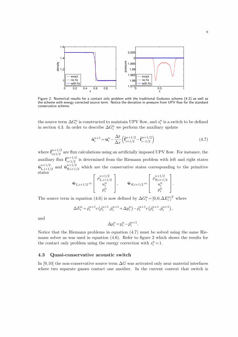
As discussed in [11], conservative schemes such as equation (4.2) can produce unphysicalbehavior near contacts. For example, figure 2 shows numerical results for a contact onlyRiemann problem with [ρ,u,p]T = [1.5,1,2] for x< 1/2 and [ρ,u,p]T = [1,1,2] for x≥ 1/2.Here we use the grid L([0,1],100) (as defined in equation (4.1)), and show results at t=0.1.The exact solution for this problem is a contact with uniform pressure and velocity (UPV)for all time. The figure shows results for both the Godnov scheme of (4.2) as well asenergy corrected scheme (4.6) with sni =1 (note that the results with sni defined using (4.8)are indistinguishable from those with sni =1 for this problem and are not presented). Thefundamental problem, that the pressure and velocity oscillate un-physically, is similar tothe problems motivating the work in [9] and [10] and so we introduce a similar energycorrection source term.

The basic energy corrected scheme takes the form

un+1i = un+1

i +sni ∆Gni . (4.6)

Here un+1i is a provisional solution determined by the usual Godunov update

un+1i =uni −

∆t

∆x

(fn+1/2i+1/2 −f

n+1/2i−1/2

),

9

0 0.2 0.4 0.6 0.8 1

1

1.2

1.4

1.6

x

de

nsity

exact

no fix

with fix

0 0.5 11.975

1.98

1.985

1.99

1.995

2

2.005

x

pre

ssu

re

exact

no fix

with fix

Figure 2: Numerical results for a contact only problem with the traditional Godunov scheme (4.2) as well asthe scheme with energy corrected source term. Notice the deviation in pressure from UPV flow for the standardconservative scheme.

the source term ∆Gni is constructed to maintain UPV flow, and sni is a switch to be definedin section 4.3. In order to describe ∆Gni we perform the auxiliary update

un+1i =uni −

∆t

∆x

(fn+1/2i+1/2 − f

n+1/2i−1/2

)(4.7)

where fn+1/2i±1/2 are flux calculations using an artificially imposed UPV flow. For instance, the

auxiliary flux fn+1/2i+1/2 is determined from the Riemann problem with left and right states

un+1/2L,i+1/2 and u

n+1/2R,i+1/2 which are the conservative states corresponding to the primitive

states

wL,i+1/2 =

ρn+1/2L,i+1/2

unipni

, wR,i+1/2 =

ρn+1/2R,i+1/2

unipni

.

The source term in equation (4.6) is now defined by ∆Gni =[0,0,∆Eni ]T where

∆Eni = ρn+1i e

(ρn+1i ,pn+1

i +∆pni)−ρn+1

i e(ρn+1i ,pn+1

i

),

and

∆pni =pni −pn+1i .

Notice that the Riemann problems in equation (4.7) must be solved using the same Rie-mann solver as was used in equation (4.6). Refer to figure 2 which shows the results forthe contact only problem using the energy correction with sni =1.

4.3 Quasi-conservative acoustic switch

In [9,10] the non-conservative source term ∆G was activated only near material interfaceswhere two separate gasses contact one another. In the current context that switch is

10

0 0.2 0.4 0.6 0.8 1

1

1.2

1.4

1.6

1.8

x

de

nsity

exact

no switch

with switch

0.3 0.4 0.5 0.6 0.7 0.81.6

1.65

1.7

1.75

1.8

1.85

1.9

x

de

nsity

exact

no switch

with switch

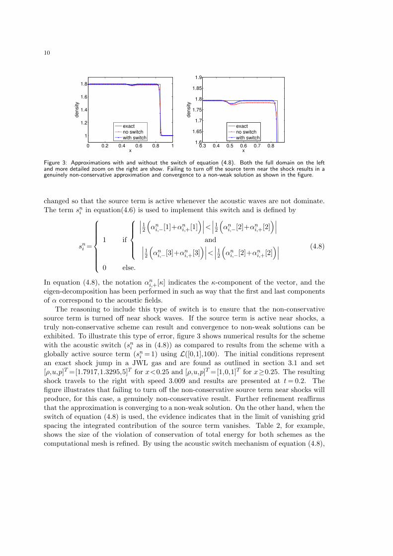
Figure 3: Approximations with and without the switch of equation (4.8). Both the full domain on the leftand more detailed zoom on the right are show. Failing to turn off the source term near the shock results in agenuinely non-conservative approximation and convergence to a non-weak solution as shown in the figure.

changed so that the source term is active whenever the acoustic waves are not dominate.The term sni in equation(4.6) is used to implement this switch and is defined by

sni =

1 if

∣∣∣12(αni,−[1]+αni,+[1]

)∣∣∣<∣∣∣12(αni,−[2]+αni,+[2]

)∣∣∣and∣∣∣12

(αni,−[3]+αni,+[3]

)∣∣∣<∣∣∣12(αni,−[2]+αni,+[2]

)∣∣∣

0 else.

(4.8)

In equation (4.8), the notation αni,+[κ] indicates the κ-component of the vector, and theeigen-decomposition has been performed in such as way that the first and last componentsof α correspond to the acoustic fields.

The reasoning to include this type of switch is to ensure that the non-conservativesource term is turned off near shock waves. If the source term is active near shocks, atruly non-conservative scheme can result and convergence to non-weak solutions can beexhibited. To illustrate this type of error, figure 3 shows numerical results for the schemewith the acoustic switch (sni as in (4.8)) as compared to results from the scheme with aglobally active source term (sni = 1) using L([0,1],100). The initial conditions representan exact shock jump in a JWL gas and are found as outlined in section 3.1 and set[ρ,u,p]T =[1.7917,1.3295,5]T for x<0.25 and [ρ,u,p]T =[1,0,1]T for x≥0.25. The resultingshock travels to the right with speed 3.009 and results are presented at t= 0.2. Thefigure illustrates that failing to turn off the non-conservative source term near shocks willproduce, for this case, a genuinely non-conservative result. Further refinement reaffirmsthat the approximation is converging to a non-weak solution. On the other hand, when theswitch of equation (4.8) is used, the evidence indicates that in the limit of vanishing gridspacing the integrated contribution of the source term vanishes. Table 2, for example,shows the size of the violation of conservation of total energy for both schemes as thecomputational mesh is refined. By using the acoustic switch mechanism of equation (4.8),

11

m energy gain without switch energy gain with switch

101 3.1383e−2 8.0240e−5

201 3.1399e−2 4.4719e−5

401 3.1384e−2 2.3977e−5

801 3.1389e−2 1.2725e−5

1601 3.1384e−2 6.5999e−6

3201 3.1382e−2 3.4031e−6

6401 3.1381e−2 1.8038e−6

12801 3.1381e−2 9.6341e−7

Table 2: Total energy gain by the scheme with and without the acoustic switch for a single shock Riemannproblem where m is the number of grid cells.

the violation of energy conservation approaches zero as the mesh is refined and so in thelimit, a conservative result is obtained. We call such schemes quasi-conservative. For allsubsequent results the acoustic switch in (4.8) is used to define sni .

5 Numerical results

We now provide a simple numerical example to illustrate that the quasi-conservativescheme of (4.6) behaves favorably in relation to the conservative scheme of (4.2) in anumber of important ways. First, (4.6) produces results which are devoid of oscillationsin the pressure and velocity even near contacts while (4.2) does not. Secondly the con-vergence rates for the two methods is investigated near the shock of a Riemann problem.The quasi-conservative scheme (4.6) is found to converge as O(∆x) while the conser-vative scheme (4.2) is found to converge at O(∆x2/3). Consider the Riemann problem[ρ,u,p]T =[0.5,0,1]T for x<0 and [ρ,u,p]T =[1,0,2]T for x≥0. Recall that the full model,including EOS parameters, is given in section 2. The computational domain for this inves-tigation is given as L([−5,5],m), and numerical integration is carried out to a final timetf = 1.5. The exact solution is approximated to a small tolerance through the methodsdescribed in section 3 and is used as a basis for comparison as needed. For this case, theexact solution consists of a left moving shock, a left moving contact, and a right movingrarefaction wave.

The numerical approximation found by the conservative Godunov method (4.2) withm= 200, is shown in figure 4. For this approximation, the pressure is not uniform inthe ∗-region and the velocity seems to jump across the material contact. Figure 5 showsthe solution to the same problem using the quasi-conservative scheme (4.6). Clearly thesolution behavior across the contact in the ∗-regions is substantially better than the cor-responding fully conservative results in figure 4. Also note that the shock lags behind theexact location for the fully conservative result, while the quasi-conservative result shows

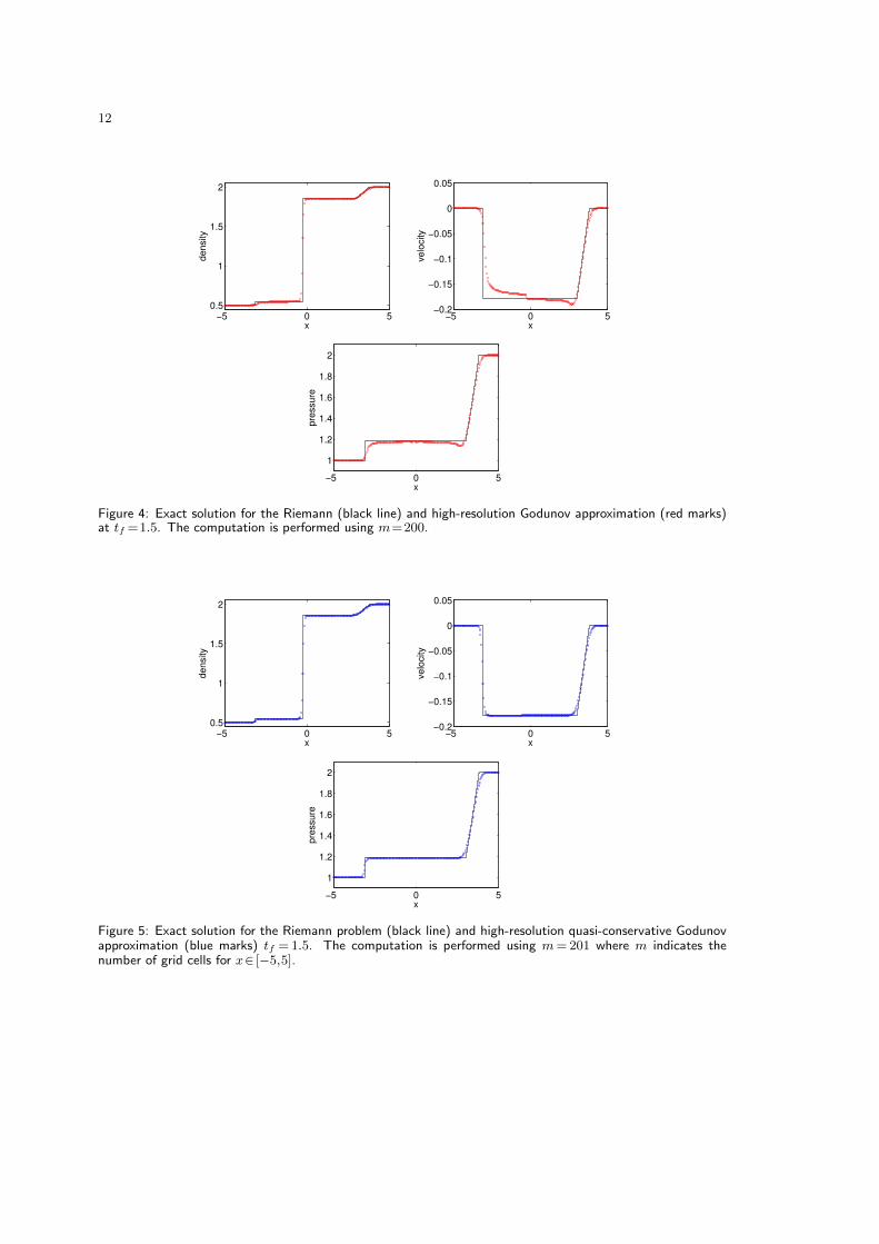
12

−5 0 50.5

1

1.5

2

x

de

nsity

−5 0 5−0.2

−0.15

−0.1

−0.05

0

0.05

x

ve

locity

−5 0 5

1

1.2

1.4

1.6

1.8

2

x

pre

ssu

re

Figure 4: Exact solution for the Riemann (black line) and high-resolution Godunov approximation (red marks)at tf =1.5. The computation is performed using m=200.

−5 0 50.5

1

1.5

2

x

de

nsity

−5 0 5−0.2

−0.15

−0.1

−0.05

0

0.05

x

ve

locity

−5 0 5

1

1.2

1.4

1.6

1.8

2

x

pre

ssu

re

Figure 5: Exact solution for the Riemann problem (black line) and high-resolution quasi-conservative Godunovapproximation (blue marks) tf =1.5. The computation is performed using m=201 where m indicates thenumber of grid cells for x∈ [−5,5].

13

the approximate shock directly atop the exact location.

We now perform a convergence study and measure the L1 convergence of the solutionin the vicinity of the shock. The exact shock propagation velocity is found to be D≈−2.08and so at t=1.5 the shock location is x≈−3.11. We calculate the L1 error in the solutionfor x∈[−3.2,−3] so that we measure convergence near the shock only. Note that the exactsolution is found to much higher tolerances than the three decimals indicated above.

m eρ(m) rate eu(m) rate ep(m) rate

201 3.88e−3 – 1.47e−2 – 1.54e−2 –

401 3.41e−3 0.19 1.29e−2 0.19 1.36e−2 0.18

801 2.84e−3 0.26 1.07e−2 0.27 1.13e−2 0.27

1601 1.78e−3 0.67 6.70e−3 0.68 7.10e−3 0.67

3201 1.19e−3 0.58 4.50e−3 0.57 4.76e−3 0.58

6401 7.94e−4 0.58 3.00e−3 0.58 3.17e−3 0.59

12801 4.91e−4 0.69 1.86e−3 0.69 1.96e−3 0.69

25601 3.17e−4 0.63 1.20e−3 0.63 1.26e−3 0.64

51201 2.02e−4 0.65 7.66e−4 0.65 8.07e−4 0.64

102401 1.30e−4 0.64 4.92e−4 0.64 5.18e−4 0.64

204801 8.29e−5 0.65 3.14e−4 0.65 3.30e−4 0.65

Table 3: Convergence results for the fully conservative scheme. Shown here are L1 errors near the shock forx∈ [−3,3.2].

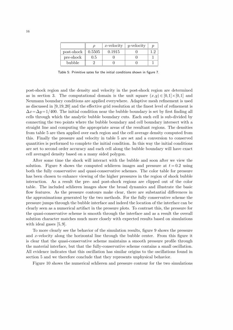
The results for the conservative scheme, shown in table 3, indicate that for all quan-tities the convergence near the shock is tending towards O(∆x2/3), the expected rate of

convergence for a 2nd order high-resolution scheme near contacts [25]. The implication isthat the convergence characteristics of the approximations near the contact have influencedthe global convergence behavior.

Table 4 shows the L1 errors for x∈ [−3.2,−3] for the quasi-conservative scheme. Alsoshown in this table is the increase in total energy over the entire domain. In contrast to theprevious results for the conservative scheme, the convergence rate here is tending towardO(∆x) for all state variables and the resultant errors are commensurately smaller. Thatis to say that the quasi-conservative scheme not only appears to provide better qualitativeapproximations as shown by figures 4 and 5, the measured convergence rate near theshock is more rapid than for the fully conservative scheme. Also notice that the violationof total energy conservation approaches zero at the rate of O(∆x2/3) which indicates thatthe contact dominates the non-conservative process.

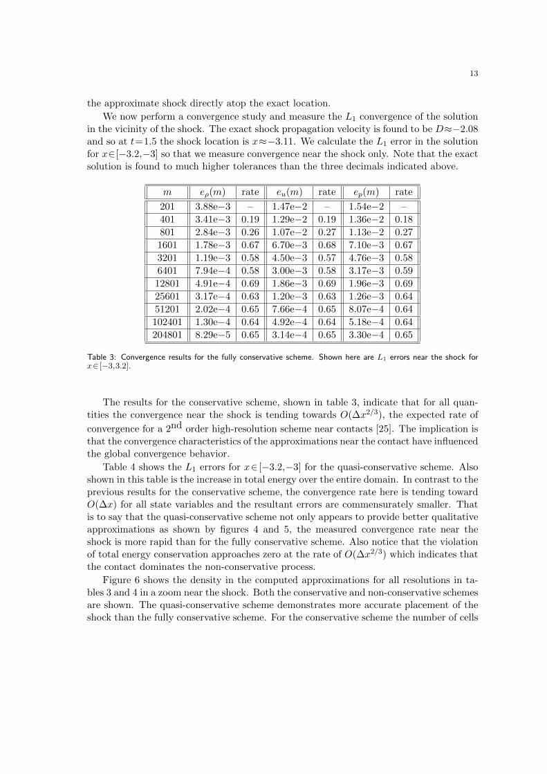
Figure 6 shows the density in the computed approximations for all resolutions in ta-bles 3 and 4 in a zoom near the shock. Both the conservative and non-conservative schemesare shown. The quasi-conservative scheme demonstrates more accurate placement of theshock than the fully conservative scheme. For the conservative scheme the number of cells

14

m eρ(m) rate eu(m) rate ep(m) rate total energy gain rate

201 2.23e−3 – 8.45e−3 – 8.87e−3 – 1.25e−1 –

401 1.77e−3 0.33 6.73e−3 0.33 6.96e−3 0.35 8.05e−2 0.63

801 9.73e−4 0.86 3.70e−3 0.86 3.84e−3 0.86 5.15e−2 0.64

1601 5.19e−4 0.91 1.98e−3 0.90 2.04e−3 0.91 3.28e−2 0.65

3201 2.55e−4 1.0 9.71e−4 1.0 1.00e−3 1.0 2.08e−2 0.66

6401 1.24e−4 1.0 4.72e−4 1.0 4.89e−4 1.0 1.32e−2 0.66

12801 6.66e−5 0.90 2.54e−4 0.89 2.61e−4 0.91 8.33e−3 0.66

25601 3.33e−5 1.0 1.27e−4 1.0 1.31e−4 0.99 5.27e−3 0.66

51201 1.65e−5 1.0 6.32e−5 1.0 6.50e−5 1.0 3.32e−3 0.67

102401 8.27e−6 1.0 3.16e−5 1.0 3.25e−5 1.0 2.10e−3 0.66

204801 4.08e−6 1.0 1.55e−5 1.0 1.60e−5 1.0 1.33e−3 0.66

Table 4: Convergence results for the quasi-conservative scheme. Shown here are L1 errors near the shock forx∈ [−3,3.2]. Also shown in this table is the increase in total energy over the entire domain.

by which the numerical shock is misplaced increases as a function of resolution. That is tosay that in the limit of vanishing grid spacing, the conservative numerical approximationwill misplace the shock by an infinite number of grid cells although the method is conver-gent in an L1 sense. The situation for the non-conservative scheme is much different inthat the approximate solutions correctly locate the shock for all resolutions. By this wemean that the analytic shock location lies in the transition region of the approximationsfor all resolutions. Successive refinement then serves only to sharpen the jump and so thescheme converges as O(∆x).

6 Practical implications

It is important to appreciate when the issues discussed in section 5 arise in practice andto gain insight as to what types of errors might be expected. To that end we investigatea test problem concerning shock interaction with a two-dimensional cylindrical bubble ofhigher density material. The single component Euler equations in two dimensions withthe JWL equation of state are used with the parameters from table 1 used to define theEOS. The extension of the one-dimensional model to two dimensions is straightforwardand can be seen for instance in [9, 16]. The extension of the numerical methods is alsostraightforward [9, 10].

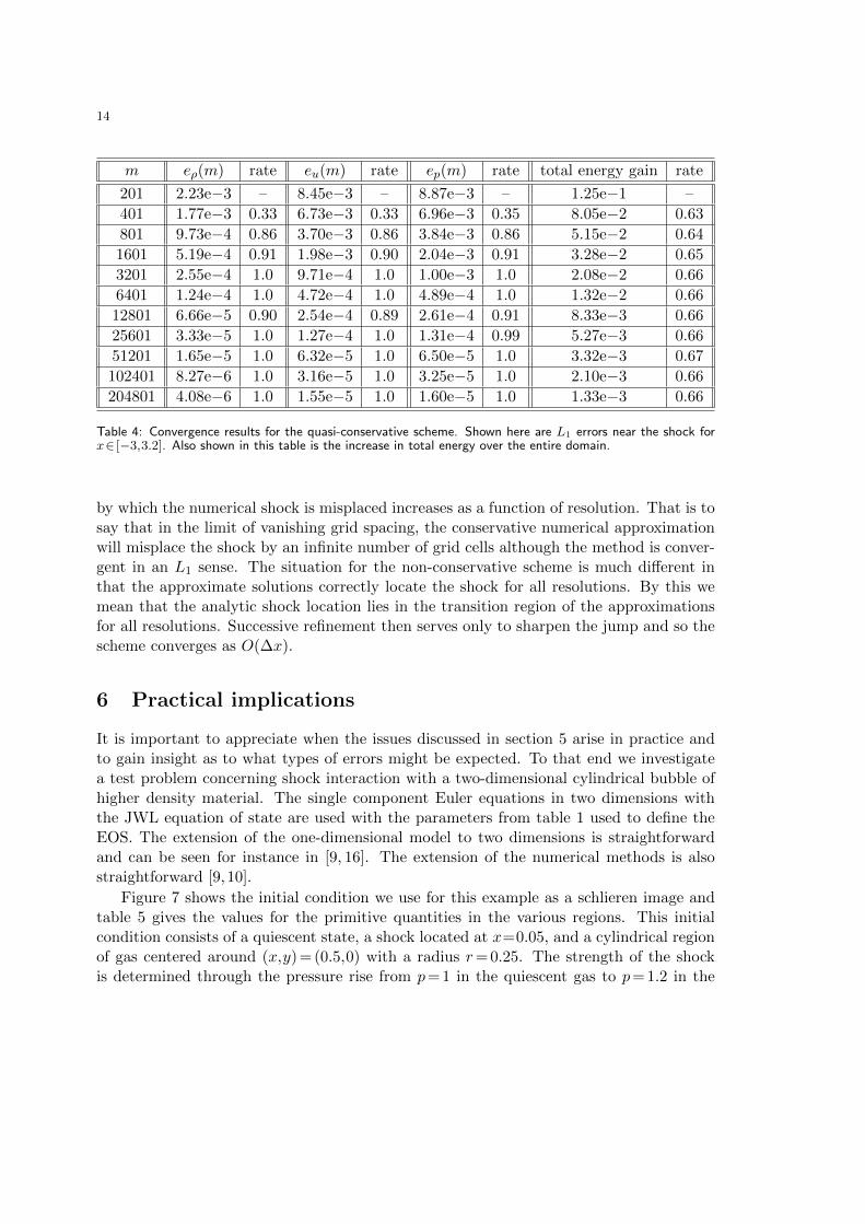
Figure 7 shows the initial condition we use for this example as a schlieren image andtable 5 gives the values for the primitive quantities in the various regions. This initialcondition consists of a quiescent state, a shock located at x=0.05, and a cylindrical regionof gas centered around (x,y) = (0.5,0) with a radius r= 0.25. The strength of the shockis determined through the pressure rise from p= 1 in the quiescent gas to p= 1.2 in the

15

−3.2 −3.15 −3.1 −3.05 −30.49

0.5

0.51

0.52

0.53

0.54

0.55

x

de

nsity

−3.2 −3.15 −3.1 −3.05 −30.49

0.5

0.51

0.52

0.53

0.54

0.55

x

de

nsity

Figure 6: Computed approximations for the density. The black line is the exact solution and the marks theapproximations. Numerical results were obtained using the fully conservative scheme (4.2) on the left and thequasi-conservative scheme (4.6) on the right with m=200,400,...,204800.

shock

interface

Figure 7: Initial conditions, shown as a numerical schlieren images, for the interaction of a shock with a bubbleof higher density material.

16

ρ x-velocity y-velocity p

post-shock 0.5505 0.1915 0 1.2

pre-shock 0.5 0 0 1

bubble 2 0 0 1

Table 5: Primitive sates for the initial conditions shown in figure 7.

post-shock region and the density and velocity in the post-shock region are determinedas in section 3. The computational domain is the unit square (x,y) ∈ [0,1]×[0,1] andNeumann boundary conditions are applied everywhere. Adaptive mesh refinement is usedas discussed in [9,19,20] and the effective grid resolution at the finest level of refinement is∆x=∆y=1/400. The initial condition near the bubble boundary is set by first finding allcells through which the analytic bubble boundary cuts. Each such cell is sub-divided byconnecting the two points where the bubble boundary and cell boundary intersect with astraight line and computing the appropriate areas of the resultant regions. The densitiesfrom table 5 are then applied over each region and the cell average density computed fromthis. Finally the pressure and velocity in table 5 are set and a conversion to conservedquantities is performed to complete the initial condition. In this way the initial conditionsare set to second order accuracy and each cell along the bubble boundary will have exactcell averaged density based on a many sided polygon.

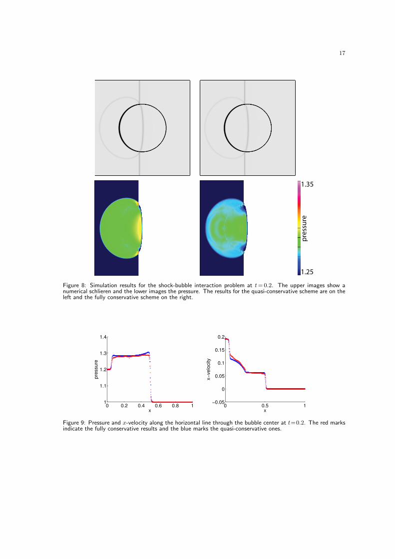
After some time the shock will interact with the bubble and soon after we view thesolution. Figure 8 shows the computed schlieren images and pressure at t= 0.2 usingboth the fully conservative and quasi-conservative schemes. The color table for pressurehas been chosen to enhance viewing of the higher pressures in the region of shock bubbleinteraction. As a result the pre- and post-shock regions are clipped out of the colortable. The included schlieren images show the broad dynamics and illustrate the basicflow features. As the pressure contours make clear, there are substantial differences inthe approximations generated by the two methods. For the fully conservative scheme thepressure jumps through the bubble interface and indeed the location of the interface can beclearly seen as a numerical artifact in the pressure plots. To contrast this, the pressure forthe quasi-conservative scheme is smooth through the interface and as a result the overallsolution character matches much more closely with expected results based on simulationswith ideal gases [5, 9].

To more clearly see the behavior of the simulation results, figure 9 shows the pressureand x-velocity along the horizontal line through the bubble center. From this figure itis clear that the quasi-conservative scheme maintains a smooth pressure profile throughthe material interface, but that the fully-conservative scheme contains a small oscillation.All evidence indicates that this oscillation has similar origins to the oscillations found insection 5 and we therefore conclude that they represents unphysical behavior.

Figure 10 shows the numerical schlieren and pressure contour for the two simulations

17

pre

ssu

re

1.25

pre

ssu

re

1.25

1.35

Figure 8: Simulation results for the shock-bubble interaction problem at t=0.2. The upper images show anumerical schlieren and the lower images the pressure. The results for the quasi-conservative scheme are on theleft and the fully conservative scheme on the right.

0 0.2 0.4 0.6 0.8 11

1.1

1.2

1.3

1.4

x

pre

ssu

re

0 0.5 1−0.05

0

0.05

0.1

0.15

0.2

x

x−

ve

locity

Figure 9: Pressure and x-velocity along the horizontal line through the bubble center at t=0.2. The red marksindicate the fully conservative results and the blue marks the quasi-conservative ones.

18

pre

ssu

re

1.25

pre

ssu

re

0.98

1.28

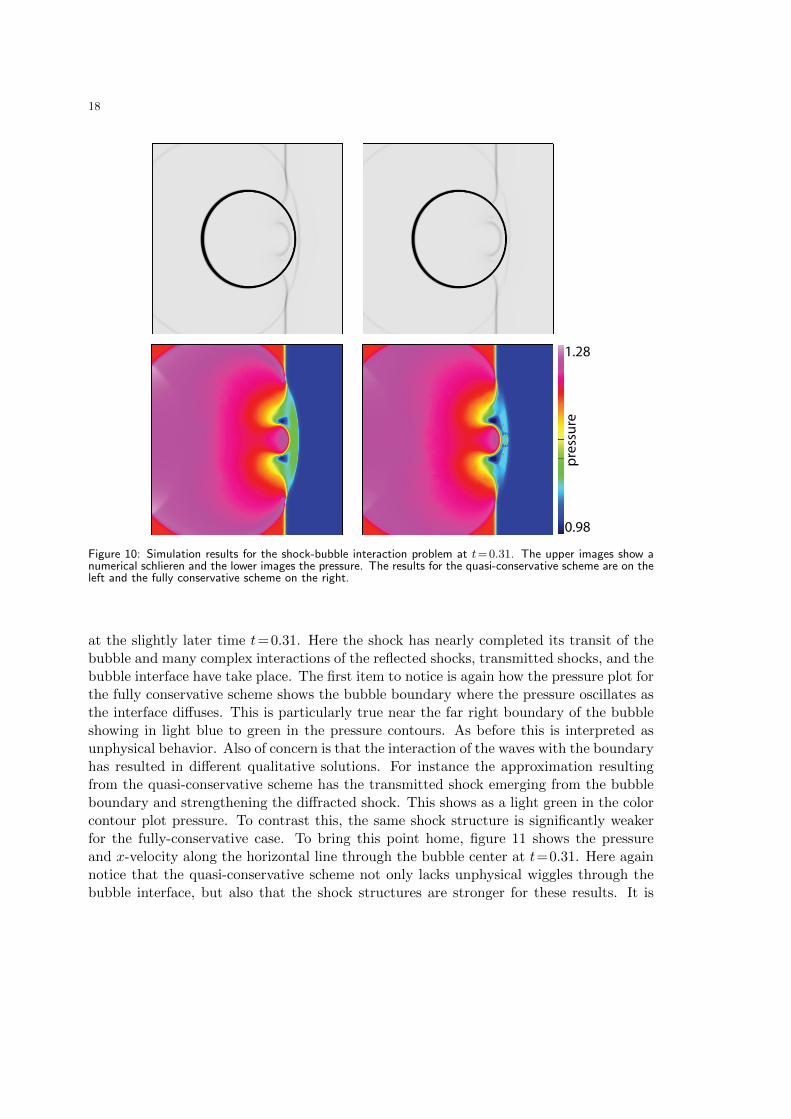
Figure 10: Simulation results for the shock-bubble interaction problem at t=0.31. The upper images show anumerical schlieren and the lower images the pressure. The results for the quasi-conservative scheme are on theleft and the fully conservative scheme on the right.

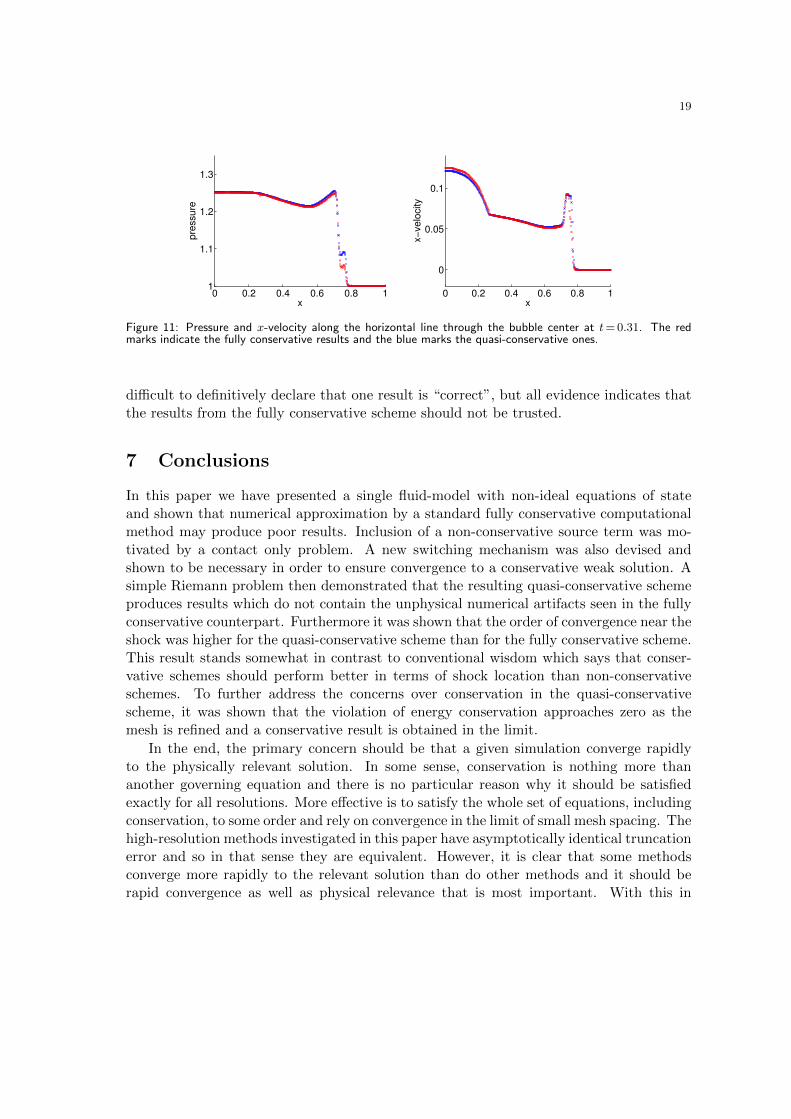
at the slightly later time t=0.31. Here the shock has nearly completed its transit of thebubble and many complex interactions of the reflected shocks, transmitted shocks, and thebubble interface have take place. The first item to notice is again how the pressure plot forthe fully conservative scheme shows the bubble boundary where the pressure oscillates asthe interface diffuses. This is particularly true near the far right boundary of the bubbleshowing in light blue to green in the pressure contours. As before this is interpreted asunphysical behavior. Also of concern is that the interaction of the waves with the boundaryhas resulted in different qualitative solutions. For instance the approximation resultingfrom the quasi-conservative scheme has the transmitted shock emerging from the bubbleboundary and strengthening the diffracted shock. This shows as a light green in the colorcontour plot pressure. To contrast this, the same shock structure is significantly weakerfor the fully-conservative case. To bring this point home, figure 11 shows the pressureand x-velocity along the horizontal line through the bubble center at t=0.31. Here againnotice that the quasi-conservative scheme not only lacks unphysical wiggles through thebubble interface, but also that the shock structures are stronger for these results. It is

19

0 0.2 0.4 0.6 0.8 11

1.1

1.2

1.3

x

pre

ssu

re

0 0.2 0.4 0.6 0.8 1

0

0.05

0.1

x

x−

ve

locity

Figure 11: Pressure and x-velocity along the horizontal line through the bubble center at t=0.31. The redmarks indicate the fully conservative results and the blue marks the quasi-conservative ones.

difficult to definitively declare that one result is “correct”, but all evidence indicates thatthe results from the fully conservative scheme should not be trusted.

7 Conclusions

In this paper we have presented a single fluid-model with non-ideal equations of stateand shown that numerical approximation by a standard fully conservative computationalmethod may produce poor results. Inclusion of a non-conservative source term was mo-tivated by a contact only problem. A new switching mechanism was also devised andshown to be necessary in order to ensure convergence to a conservative weak solution. Asimple Riemann problem then demonstrated that the resulting quasi-conservative schemeproduces results which do not contain the unphysical numerical artifacts seen in the fullyconservative counterpart. Furthermore it was shown that the order of convergence near theshock was higher for the quasi-conservative scheme than for the fully conservative scheme.This result stands somewhat in contrast to conventional wisdom which says that conser-vative schemes should perform better in terms of shock location than non-conservativeschemes. To further address the concerns over conservation in the quasi-conservativescheme, it was shown that the violation of energy conservation approaches zero as themesh is refined and a conservative result is obtained in the limit.

In the end, the primary concern should be that a given simulation converge rapidlyto the physically relevant solution. In some sense, conservation is nothing more thananother governing equation and there is no particular reason why it should be satisfiedexactly for all resolutions. More effective is to satisfy the whole set of equations, includingconservation, to some order and rely on convergence in the limit of small mesh spacing. Thehigh-resolution methods investigated in this paper have asymptotically identical truncationerror and so in that sense they are equivalent. However, it is clear that some methodsconverge more rapidly to the relevant solution than do other methods and it should berapid convergence as well as physical relevance that is most important. With this in

20

mind, a more practical realization of the potential problems was investigated. Here theinteraction of a shock with a 2-D cylindrical bubble of dense gas was investigated. Thefully conservative method shows results which have obvious problems in that the pressureoscillates through the bubble interface while the quasi-conservative results are in accordwith expectations. Based on the information at hand we are drawn to the conclusion thatthe approximations from the quasi-conservative method are the ones to be believed. Itshould also be stated that although the variation between the results from the differentsolution methods is relatively small, the addition of further physical processes can amplifyany differences which do exist. Chemical mechanism, for example, are often quite stiff aswell as highly non-linear and any differences in simulation results from the flow solverscan result in substantial solution differences in this regime.

Acknowledgements

This study has been supported by Lawrence Livermore National Laboratory under the aus-pices of the U.S. Department of Energy through contract number DE-AC52-07NA27344.

References

[1] P. Lax, B. Wendroff, Systems of conservation laws, Commun. Pur. Appl. Math. 13 (1960)217–237.

[2] T. Y. Hou, P. G. Le Floch, Why nonconservative schemes converge to wrong solutions: Erroranalysis, Math. Comp. 62 (206) (1994) 497–530.

[3] J. Glimm, Solutions in the large for nonlinear hyperbolic systems of equations, Commun. Pur.Appl. Math. 18 (1965) 697–715.

[4] S. Karni, Multicomponent flow calculations by a consistent primitive algorithm, J. Comput.Phys. 112 (1994) 31–43.

[5] J. J. Quirk, S. Karni, On the dynamics of a shock-bubble interaction, J. Fluid Mech. 318(1996) 129–163.

[6] R. Abgrall, How to prevent pressure oscillations in mulicomponent flow calculations: A quasiconservative approach, J. Comput. Phys. 125 (1996) 150–160.

[7] R. Saurel, R. Abgrall, A simple method for compressible multifluid flows, SIAM J. Sci. Com-put. 21 (3) (1999) 1115–1145.

[8] R. Abgrall, S. Karni, Computations of compressible multifluids, J. Comput. Phys. 169 (2001)594–623.

[9] J. W. Banks, D. W. Schwendeman, A. K. Kapila, W. D. Henshaw, A high-resolution Godunovmethod for compressible multi-material flow on overlapping grids, J. Comput. Phys. 223(2007) 262–297.

[10] J. W. Banks, W. D. Henshaw, D. W. Schwendeman, A. K. Kapila, A study of detonationpropagation and diffraction with compliant confinement, Combust. Theory and Modelling12 (4) (2008) 769–808.

[11] R. Saurel, E. Franquet, E. Daniel, O. L. Metayer, A relaxation-projection method for com-pressible flows. Part I: The numerical equation of state for the Euler equations, J. Comput.Phys. 223 (2007) 822–845.

[12] B. M. Dobratz, Properties of chemical explosives and explosive simulants, Tech. Rep. LLNLUCRL-51319, Lawrence Livermore Laboratory National Laboratory (July 1974).

21

[13] R. Menikoff, B. J. Plohr, The Riemann problem for fluid flow or real materials, Reviews ofModern Physics 61 (1) (1989) 75–130.

[14] M. Larini, R. Saurel, J. C. Loraud, An exact Riemann solver for detonation products, ShockWaves 2 (1992) 225–236.

[15] R. Saurel, M. Larini, J. C. Loraud, Exact and approximate Riemann solvers for real gases, J.Comput. Phys. 112 (1994) 126–137.

[16] G. B. Whitham, Linear and Nonlinear Waves, Wiley-Interscience, New York, 1974.[17] U. M. Ascher, L. R. Petzold, Computer Methods for Ordinary Differential Equations and

Differential-Algebraic Equations, SIAM, Philadelphia, 1998.[18] A. K. Kapila, D. W. Schwendeman, J. B. Bdzil, W. D. Henshaw, A study of detonation

diffraction in the Ignition-and-Growth model, Combust. Theory and Modelling 11 (5) (2007)781–822.

[19] W. D. Henshaw, D. W. Schwendeman, An adaptive numerical scheme for high-speed reactiveflow on overlapping grids, J. Comput. Phys. 191 (2) (2003) 420–447.

[20] W. D. Henshaw, D. W. Schwendeman, Moving overlapping grids with adaptive mesh refine-ment for high-speed flow, J. Comput. Phys. 216 (2) (2006) 744–779.

[21] S. K. Godunov, Finite difference method for numerical computation of discontinuous solutionsof the equations of fluid dynamics, Mat. Sb. 47 (1959) 271–306.

[22] B. van Leer, Towards the ultimate conservative difference scheme, V. A second-order sequelto Godunov’s method, J. Comput. Phys. 32 (1979) 101–136.

[23] E. F. Toro, Riemann Solvers and Numerical Methods for Fluid Dynamics, Springer, Berlin,1999.

[24] P. Glaister, An approximate linearised riemann solver for euler equations for real gases, J.Comput. Phys. 74 (1988) 382–408.

[25] J. W. Banks, T. Aslam, W. J. Rider, On sub-linear convergence for linearly degenerate wavesin capturing schemes, J. Comput. Phys. 227 (14) (2008) 6985–7002.